1

Always and Everywhere Inflation? Treasuries Variance

Decomposition and the Impact of Monetary Policy

Alexandros Kontonikas§, Charles Nolan

and Zivile Zekaite

‡

Adam Smith Business School, University of Glasgow

October 2015

Abstract

This paper investigates the sources of variation in Treasury bonds returns and the role of

monetary policy over the last three decades. Firstly, we decompose unexpected excess returns

on 2-, 5- and 10-year Treasuries in three components related to revisions in expectations

(news) about future excess returns, inflation and real interest rates. Our results indicate that

inflation news is the key driver of Treasuries returns. Secondly, we evaluate the impact of

conventional and unconventional monetary policy on Treasuries returns and their

components. The monetary policy impact on the Treasury market is largely explained

through revisions in inflation expectations.

Keywords: Bond Market Variance Decomposition; Monetary Policy; Financial Crisis.

JEL classification: G12; G01; E44; E52.

§ Corresponding author. Prof. Alexandros Kontonikas, Adam Smith Business School, Accounting and Finance

Subject area, University of Glasgow, Glasgow, G12 8QQ, UK, alexandros.kontonikas@glasgow.ac.uk, Tel. +44

(0) 1413306866. Prof. Charles Nolan, Adam Smith Business School, Economics Subject Area, University of Glasgow,

Glasgow, G12 8QQ, UK, charles.nolan@glasgow.ac.uk, Tel. +44 (0) 1413308693. ‡ Zivile Zekaite, Adam Smith Business School, Economics Subject Area, University of Glasgow, Glasgow, G12

8QQ, UK, z.zekaite.1@research.gla.ac.uk, Tel. +44 (0) 1413308544.

We would like to thank J. Ammer, C. Burnside, J. Campbell, J. Cochrane, A. Duncan, C. Favero, C. Florackis,

A. Kostakis, conference participants at the 2015 SIRE Asset Pricing Conference, the 2015 Money Macro and

Finance Conference, the 2015 Scottish Area Group BAFA Conference and the 4th UECE Conference on

Economic and Financial Adjustments, and seminar participants at the Queen’s University Management School

and the Lisbon School of Economics and Management for useful comments and suggestions. We would also

like to thank Tom Doan for helpful advice on the estimation code.

2

1. Introduction

The greatest part of the three-decade long bull-run in Treasuries took place within an

environment of low and stable inflation and sustained economic growth. Starting from the

mid-1980s, the macroeconomic tranquillity that defined the Great Moderation era was

accompanied by—some argue delivered by—an apparently simple and predictable rule

underlying the conduct of monetary policy, based upon targeting of the Federal funds rate

(FFR). That era of stability and predictability came to an abrupt end with the global financial

crisis of 2007-2009. As the zero lower bound on interest rates constrained policymakers in

the US and elsewhere, conventional monetary policy was unable to boost economic activity.

The Federal Reserve (Fed) adopted non-conventional policy tools, including liquidity

facilities and outright purchases of Treasury bonds and other assets from the private sector, in

order to improve financial market conditions and reduce longer-term interest rates. After

almost six years of unprecedented expansion in the Fed’s balance sheet, the end of

quantitative easing (QE) was announced in October 2014 raising questions about the

prospects of Treasuries in the context of the Fed’s exit plan. Understanding how Treasuries

respond to monetary actions is crucial for policy makers and investors at a global level given

the US dollar’s reserve currency status.

This study conducts an empirical investigation of the sources of variation in Treasury

bond returns and the role of monetary policy over the last three decades, thereby resting upon

two important strands of the bond market literature. The first strand includes studies that

assess the role of macroeconomic forces, most importantly inflation, in determining bond

market volatility. As Duffee (2014) notes, the significance of inflation risk for nominal bonds

within prominent term structure models varies considerably from very high (Piazzesi and

Schneider; 2007) to almost zero (Chernov and Mueller; 2012). Different restrictions on risk

premium dynamics may play a role in explaining these differences. An alternative approach

3

to conduct the assessment, not relying upon strong theoretical assumptions, uses identities

linking unexpected excess bond returns to revisions in expectations (“news”) about future

excess returns, inflation and real interest rates. News are identified using a VAR time-series

econometric model. The decomposition of returns to news terms was pioneered in bond

market studies by Campbell and Ammer (1993) who built upon Campbell and Shiller’s

(1988) and Campbell’s (1991) earlier work. Using this approach, it is commonly found that

revisions in inflation expectations account for most of the shocks to long-term government

bond returns in the US (Campbell and Ammer, 1993; Engsted and Tanggaard, 2007) and

other countries (Barr and Pesaran, 1997; Cenedese and Malluci, 2015).

The second strand of the literature considers the bond market effects of monetary

policy actions. Two key findings from earlier studies, conducted prior to the 2007-2009

financial crisis, are that Treasuries significantly respond to shifts in the FFR and the response

tends to diminish at longer maturities (Kuttner, 2001; Gurkaynak, Sack, and Swanson, 2005;

Cochrane and Piazzesi, 2002). Following the onset of the financial crisis, the implementation

of QE led to a surge of studies that examine its impact on the bond market. Using various

approaches, it is commonly found that QE was effective in reducing long-term Treasury bond

yields. As to how this was achieved, the existing literature emphasizes two potential

channels. According to the signalling channel, QE provided information to market

participants about the commitment of the Fed to easier monetary policy, leading to lower

expectations of future short-term rates. This development explains, through the expectations

theory of the term structure, the reduction in long-term yields. On the other hand, the

portfolio balance channel assumes imperfect substitutability of bonds with different

maturities, consistent with preferred habitat investors (Vayanos and Vila, 2009). According to

it, the QE-induced decline in the supply of long-term bonds reduced their yield by

compressing the term premium. The empirical evidence is rather mixed. For example,

4

Gagnon et al. (2011) and D'Amico et al. (2012) find that reductions in the yield of long-term

Treasuries primarily reflect a lower term premium, while the results of Christensen and

Rudebusch (2012) and Bauer and Rudebusch (2013) favour the signalling channel. The

mixed empirical evidence together with the empirical failure of the expectations theory

(Thornton, 2005; Sarno, Thornton and Valente, 2007) and the restrictive theoretical

assumptions underlying preferred habitat (Thornton, 2012) imply that our understanding of

how QE led to lower bond yields is still incomplete.

In this paper we take an alternative route to identify the sources of the bond market’s

response to monetary policy. To do so, we modify Bernanke and Kuttner’s (2005) extension

of Campbell and Ammer’s (1993) framework so that it is applicable to bond market returns.1

At the first stage of our analysis, we decompose unexpected excess returns on 2-, 5- and 10-

year Treasury bonds to news about future excess returns, inflation and real interest rates. At

the second stage, we evaluate the impact of conventional and unconventional monetary

policy shifts on Treasury bond returns and their components. The sample period, 1985-2014,

commences during the Great Moderation and ends in the aftermath of the recent financial

crisis. We use FFR-based measures to capture conventional policy shifts, while non-

conventional policies are captured using changes in the monetary base. The use of quantity-

based indicators is motivated by a number of recent studies that evaluate the role of the

monetary base, or the supply reserves, as an alternative operating target for monetary policy

(Curdia and Woodford, 2011; Gertler and Karadi, 2013). Thus, we contribute to the existing

literature in three important ways. First, by using an approach that allows us to explain the

bond market reaction to monetary policy shifts over the last three decades on the basis of

news about macro-fundamentals and risk. Second, by paying special attention to the role of

1 Using the VAR-based decomposition of returns to news components, Bernanke and Kuttner (2005) and Maio

(2014) examine the US stock market’s reaction to monetary policy shifts. Bredin, Hyde and O’Reilly (2010)

employ this approach to examine the pre-crisis (1994-2004) domestic and international bond market impact of

domestic monetary policy actions in the US, UK and Germany. In the case of the US, they do not find

significant effects.

5

the financial crisis and the non-conventional policies subsequently adopted by the Fed. Third,

by considering shorter maturities, in addition to the often analysed 10-year Treasury bond, in

order to examine whether the effects vary across the yield curve.

Previewing our empirical results, the main findings can be summarized as follows.

First, across different maturities, variance decomposition results show that news about future

inflation is the key factor in explaining the variability of unexpected excess Treasury bond

returns during the era of lower inflation that commenced in the mid-1980s. On the other

hand, the influence of risk premium news and real interest news is typically negligible.

Second, regarding the effect of conventional and unconventional monetary policy actions, we

find that monetary easing is generally associated with higher unexpected excess Treasury

bond returns. That said, the bond market reaction to conventional policy shocks has grown

weaker over the more recent period perhaps reflecting changes, ever since the mid-1990s, in

the way that the Fed implements and communicates monetary policy. In the case of quantity-

based monetary policy indicators, our results are driven largely by the peak of the financial

crisis in autumn 2008 when unprecedented expansion in the Fed’s balance sheet was

accompanied by a stronger bond market response to money growth. Third, our results

highlight the importance of inflation news in explaining the bond market reaction to

monetary policy. We find that the positive effect of monetary easing on unexpected excess

Treasury bond returns mainly comes from a corresponding negative effect on inflation

expectations. Fourth, the evidence is overall not supportive for the portfolio balance

mechanism’s prediction of a strong role for risk premium news in explaining the bond market

reaction to the expanding balance sheet of the Fed. These main findings are reasonably robust

to various sensitivity checks, related to the specification of the underlying VARs and the

monetary policy proxies.

6

The rest of the paper is structured as follows. Section 2 presents the methodology.

Section 3 describes the dataset, explains the proxies that we use to identify conventional and

non-conventional monetary policy actions and discusses issues related to the assumption that

the latter are exogenous. Section 4 contains the empirical results from the baseline analysis,

while Section 5 contains the robustness checks. Section 6 concludes.

2. Methodology

2.1 Excess bond returns decomposition

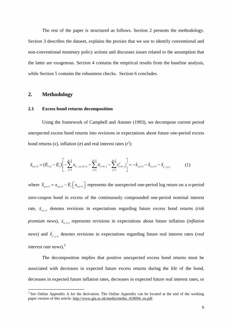
Using the framework of Campbell and Ammer (1993), we decompose current period

unexpected excess bond returns into revisions in expectations about future one-period excess

bond returns (x), inflation (π) and real interest rates (ri):

1 1 1

, 1 1 , 1 1 1 , 1 , 1 , 11 1 1

( ) i

n n ni

n t t t n j t j t j t j x t t r tj j j

x E E x r x x x

(1)

where , 1 , 1 , 1n t n t t n tx x E x represents the unexpected one-period log return on a n-period

zero-coupon bond in excess of the continuously compounded one-period nominal interest

rate, , 1x tx

denotes revisions in expectations regarding future excess bond returns (risk

premium news), , 1tx

represents revisions in expectations about future inflation (inflation

news) and , 1ir t

x

denotes revisions in expectations regarding future real interest rates (real

interest rate news).2

The decomposition implies that positive unexpected excess bond returns must be

associated with decreases in expected future excess returns during the life of the bond,

decreases in expected future inflation rates, decreases in expected future real interest rates, or

2 See Online Appendix A for the derivation. The Online Appendix can be located at the end of the working

paper version of this article: http://www.gla.ac.uk/media/media_418694_en.pdf.

7

a combination of the three. Equation (1) is a dynamic accounting identity that arises from the

definition of bond returns and imposes internal consistency on expectations.3 It is not a

behavioural model containing economic theory and asset pricing assumptions. Nevertheless,

both the Fisher hypothesis and the expectations theory of the term structure have important

implications for the decomposition of excess bond returns. Specifically, the former

hypothesis implies that ex ante real interest rates are constant and therefore the real interest

rate news term is zero. The latter hypothesis assumes time-invariant expected excess bond

returns which are consistent with the risk premium news term being zero. Therefore, in the

extreme, if both hypotheses hold, inflation news will be the only source of variation in bond

returns in excess of the short-term risk-free rate.4

From Equation (1) it follows that the total variance of excess returns can be

decomposed into the sum of the three variances plus the respective covariance terms:

, 1 , 1 , 1 , 1 , 1, 1

, 1 , 1, 1 , 1

2 ,

2 , 2 ,

i

i i

n t x t t x t tr t

x t tr t r t

Var x Var x Var x Var x Cov x x

Cov x x Cov x x

(2)

In order to evaluate the relative importance of news about risk premium, inflation and

real interest rates, we normalise each of the variance and covariance terms in Equation (2) by

the total variability of excess returns. The delta method is used to calculate the standard errors

for the terms of the variance decomposition since these are nonlinear functions of the

estimated VAR parameters.5

3 Note that in the case of zero-coupon bonds the dynamic accounting identity holds exactly.

4 Existing evidence regarding the empirical validity of the expectations hypothesis and the Fisher hypothesis can

be described as mixed with the role of the adopted testing procedures being crucial. Sarno, Thornton and

Valente (2007) use a more powerful test with either macroeconomic factors or more than two bond yields and

overturn evidence from conventional tests by showing that the expectations hypothesis can be rejected

throughout the maturity spectrum. Christopoulos and Leon-Ledesma (2007) attribute the lack of widespread

empirical evidence for the Fisher hypothesis in cointegration-based studies to non-linearities in the long-run

relationship between nominal interest rates and inflation. 5 This approach is also employed by Campbell and Ammer (1993), Barr and Pesaran (1997) and Bernanke and

Kuttner (2005).

8

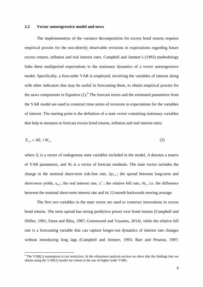
2.2 Vector autoregressive model and news

The implementation of the variance decomposition for excess bond returns requires

empirical proxies for the non-directly observable revisions in expectations regarding future

excess returns, inflation and real interest rates. Campbell and Ammer’s (1993) methodology

links these multiperiod expectations to the stationary dynamics of a vector autoregressive

model. Specifically, a first-order VAR is employed, involving the variables of interest along

with other indicators that may be useful in forecasting them, to obtain empirical proxies for

the news components in Equation (1).6 The forecast errors and the estimated parameters from

the VAR model are used to construct time series of revisions in expectations for the variables

of interest. The starting point is the definition of a state vector containing stationary variables

that help to measure or forecast excess bond returns, inflation and real interest rates:

1 1t t tZ AZ W (3)

where Zt is a vector of endogenous state variables included in the model, A denotes a matrix

of VAR parameters, and Wt is a vector of forecast residuals. The state vector includes the

change in the nominal short-term risk-free rate, ∆y1,t ; the spread between long-term and

short-term yields, sn,t ; the real interest rate, rti ; the relative bill rate, rbt , i.e. the difference

between the nominal short-term interest rate and its 12-month backwards moving average.

The first two variables in the state vector are used to construct innovations in excess

bond returns. The term spread has strong predictive power over bond returns (Campbell and

Shiller, 1991; Fama and Bliss, 1987; Greenwood and Vayanos, 2014), while the relative bill

rate is a forecasting variable that can capture longer-run dynamics of interest rate changes

without introducing long lags (Campbell and Ammer, 1993; Barr and Pesaran, 1997;

6 The VAR(1) assumption is not restrictive. In the robustness analysis section we show that the findings that we

obtain using the VAR(1) model are robust to the use of higher order VARs.

9

Bernanke and Kuttner, 2005). The VAR estimates allow us to compute unexpected excess

bond returns and the three components identified in Equation (1) as follows:

, 1 1 1 2 1( 1)( )T T

n t t tx n s W s W , (4)

1

3 1, 1( ) ( )i

T n

tr tx s I A A A W

, (5)

1 1

, 1 1 1 , 11 i

T n

t t r tx s I A n I I A A A W x

, (6)

, 1 , 1 , 1, 1ix t n t tr tx x x x

. (7)

where siT is a unit vector with i representing i

th equation in the model and accordingly the i

th

element of a vector is set to 1; I is the identity matrix.7

Equation (4) shows that current unexpected excess bond returns are obtained using

innovations in the change of the nominal short-term rate and the term spread. The inclusion

of the real interest rate in the state vector allows the extraction of news about it directly from

the model as indicated by Equation (5). In Equation (6), the inflation news term is computed

by combining innovations in the change of the nominal short-term rate with news about real

interest rates. Finally, Equation (7) shows that risk premium news is obtained as a residual

using the dynamic accounting identity and the estimates of the other components. Backing

out risk premium news as a residual is necessary for zero-coupon bonds since shrinking

maturity over the life of a bond precludes the direct forecasting of excess returns using the

VAR model. Hence, excess bond returns are not directly included in the VAR and the related

news component is backed out as a residual term. As Engsted, Pedersen and Tanggaard

(2012) explain, the need to account for shrinking maturities is crucial within this framework.

7 See Online Appendix B for more details.

10

Ignoring this may lead to unwarranted conclusions about the reliability of the bond market

variance decomposition, as in Chen and Zhao (2009).8

The VAR model that is used to extract news is assumed to contain all relevant

information that investors may have when forming expectations about the future. Given

variability in the components of excess bond returns, the variance decomposition is indeed

conditional upon this information. If investors have additional information that is not present

in the state vector, the relative importance of the residual component (risk premium news in

our analysis) may be overstated.9 In the robustness analysis section we show that our baseline

findings, based on the state vector described above, are robust to the incorporation of

additional macro-financial predictor variables in the state vector.

2.3 Monetary policy effects

The above sections explain how the variation of the unexpected excess bond returns

can be linked to news about future excess returns, inflation and real interest rates, and how

these news terms can be obtained from a VAR model. In this section we present the

framework that we use to estimate the impact of monetary policy actions on the bond market.

To do so, we modify Bernanke and Kuttner’s (2005) extension of Campbell and Ammer’s

(1993) methodology for the case of the bond market. 10

Our approach generates estimates of

8 Chen and Zhao (2009) decompose unexpected excess bond returns in two components: cash flow news and

risk premium news, where the former is backed out as a residual from the VAR estimation. Since nominal cash

flows of Treasury bonds are fixed, the estimated cash flows news must only be reflecting modelling noise, while

real interest or inflation shocks will be incorporated in discount rate news. They find, however, that the

estimated variance of cash flows news is not zero, or even smaller than that of discount rate news, and attribute

this to missing state variables in the discount rate forecast. However, as Engsted, Pedersen and Tanggaard

(2012) point out, Chen and Zhao (2009) neglect the shrinking maturity of the bonds over their lifetime.

Furthermore, while they use excess bond returns in the VAR, the formula that they use for the decomposition

holds for raw returns only. 9 Campbell and Ammer (1993) point out that the sign of the possible bias is uncertain since it will depend on the

covariances between state variables and any omitted variables. 10

Bredin, Hyde and O’Reilly (2010) also consider the impact of monetary policy actions on bond returns and

their components using Bernanke and Kuttner’s (2005) VAR-based approach. Their analytical framework,

however, is different from ours since their formulas that they use for the decompositions of bond returns apply

to the case of infinite maturity coupon bonds. Moreover, they include excess returns directly in the VAR and

back out inflation news as a residual term.

11

the impact of monetary policy actions on unexpected excess bond returns and the related

news terms, thereby providing insights to sources of the bond market’s response to monetary

policy. The starting point is the inclusion of a monetary policy indicator (MP) as an

exogenous variable in the VAR model:

*

1 1 1t t t tZ AZ MP W (8)

where is a vector that includes the state variables’ response parameters to

contemporaneous monetary policy actions. As we explain in Section 3.3, we employ four

alternative monetary policy indicators that relate to actual and surprise changes in the policy

rate and the quantity of money.

The original VAR error vector 1tW in Equation (3) is decomposed in a component

related to the monetary policy actions, 1tMP , and a component related to other information,

*

1tW . We proceed by estimating the original VAR model to obtain estimates of A and then

regress the forecast residuals vector on the monetary policy indicator variable in order to

estimate . The monetary policy effect on the current unexpected excess returns and news

about real interest rates, inflation and the risk premium can be computed using Equations (9)-

(12), respectively:11

, 1 1 2( 1)( )MP T T

n tx n s s (9)

1

3, 1( ) ( )i

MP T n

r tx s I A A A

(10)

1 11

, 1 3 1( ) ( ) 1MP T n T n

tx s I A A A s I A n I I A A A

(11)

, 1 , 1 , 1 , 1i

MP MP MP MP

x t n t t r tx x x x

(12)

11 To obtain Equations (9)-(11), Wt+1 is replaced with *

1 1t tMP W in Equations (4)-(6) and then partial

derivatives with respect to MPt+1 are taken.

12

Thus, the response of excess bond returns and their components to monetary policy

actions depends both on and the dynamics of the VAR through A. As in Bernanke and

Kutner (2005), the delta method is used to compute standard errors for these responses.

3. Data and variables

3.1 Sample period

We use monthly data over the period 1985:1 – 2014:2. Our sample commences during

the early years of the Great Moderation period, while its latter part contains the recent global

financial crisis and its aftermath. Our estimations are conducted over both the full sample

period (1985:1 – 2014:2) and a shorter sample (1985:1 – 2007:7) that ends prior to the onset

of the recent financial crisis.12

Doing so, we get insights about the impact of crisis on the

variance decomposition of unexpected excess bond returns and the relationship between

monetary policy actions and bond returns.

3.2 VAR state variables

We use the 1-month Treasury bill rate, obtained from the Centre for Research in

Security Prices (CRSP), as a proxy for the nominal short-term risk-free interest rate (y1,t). The

long-short spread (sn,t) is calculated as the difference between 10-, 5-, and 2- year zero-

coupon Treasury bond yields and y1,t. Data on continuously compounded zero-coupon yields

is obtained from the daily dataset provided by Gurkaynak, Sack, and Wright (2007).13

The ex

post real interest rate is defined as the difference between y1,t-1 and the current monthly

inflation rate, measured by the change in the log of the seasonally adjusted CPI All items

index. CPI data is provided by the Federal Reserve Bank of St Louis (FREDII database). The

12

The start of the financial crisis is dated to August 2007 when doubts about global financial stability emerged

and the first major central bank interventions in response to increasing interbank market pressures took place

(Brunnermeier, 2009; Kontonikas, MacDonald and Saggu, 2013). 13

The dataset is available online at http://www.federalreserve.gov/pubs/feds/2006/200628/200628abs.html.

13

relative bill rate is the deviation of y1,t from its 12-month backwards moving average. All

state variables are demeaned prior to estimations and expressed in percentages per annum on

continuously compounded basis (end of month data used).

3.3 Monetary policy indicators

Both the Fed’s operating procedures and the underlying macro-financial environment

have changed over time. By the early 1980s, Volcker’s disinflation was largely accomplished

with inflation sharply reduced to around 3% at 1983. This development allowed interest rates

to decline and eventually ushered the Great Moderation era that was characterised by overall

macroeconomic stability. Monetary policy conduct during that period was characterised by

FFR targeting and increasing transparency, with the Fed announcing the decision for the

target FFR after each FOMC meeting since February 1994.14

The financial crisis of 2007-

2009 brought this benign regime to an end and had a significant impact on the Fed’s approach

to monetary policy implementation. The Fed responded aggressively to the crisis by reducing

the target FFR to near zero. Moreover, it used various tools (liquidity facilities and Large

Scale Asset Purchases (LSAPs)) to improve financial market conditions and put downward

pressure on longer-term interest rates, thereby supporting economic activity.15

Conducting the LSAPs programme, the Fed purchased significant amounts of longer-

term assets from the private sector, mainly Treasury bonds and agency mortgage backed

14

US monetary policy operating procedures have included periods of targeting the FFR, i.e. the interest rate on

overnight loans of reserves between banks, (1972–79 and 1988–present), non-borrowed reserves targeting

(1979–82) and borrowed reserves targeting (1982–88). There is substantial empirical evidence indicating that

the FFR is the key US monetary policy indicator during both the pre-1979 and post-1982 periods (Bernanke and

Blinder, 1992; Bernanke and Mihov, 1998; Romer and Romer, 2004). 15

These included (i) the provision of short-term term liquidity to banks and other financial institutions through

discount window lending and other facilities, such as the Term Auction Facility; (ii) the direct provision of

liquidity to borrowers and investors in important credit markets via e.g. the Commercial Paper Funding Facility;

(iii) the Large Scale Asset Purchases programme that aimed to support credit markets and improve overall

financial conditions. See Table C2 in Online Appendix C for a list of the relevant announcements by the Fed.

14

securities, leading to significant changes in the size and composition of its balance sheet.16

The increase in the Fed’s assets was matched by an expansion in its liabilities. Particularly,

reserve balances have increased considerably relative to their level prior to the financial crisis

and are highly in excess of the regulatory requirements. Reserves became the main

component of the monetary base since currency in circulation continued to exhibit an only

gradual increase over time. Figure 1 shows the dramatic rise in total reserves and the

monetary base since late 2008 and also highlights that, in contrast to narrow money, broad

money (M2) did not significantly expand. The lack of a dramatic shift in broader monetary

aggregates is related to the fact that banks let their levels of excess reserves to increase

sharply (Fawley and Neely, 2013). Fama (2013) attributes this development to the payment

of interest on excess reserves by the Fed since October 2008 which implies that they no

longer impose a cost on banks. These developments renewed the focus of central bankers and

monetary economists to quantity-based policy indicators with a number of recent theoretical

(Curdia and Woodford, 2011; Gertler and Karadi, 2013) and empirical studies (Gambacorta,

Hofmann and Peersman, 2014) investigating the macroeconomic role of LSAPs and

evaluating the monetary base, or the supply of reserves, as an alternative operating target.

[FIGURE 1 HERE]

In our empirical analysis we use four monetary policy indicators that are related to

actual and unexpected changes in the FFR and the (log) monetary base. Interest rate-based

measures are capturing conventional monetary policy, while non-conventional policy

dimensions are captured by quantity-based measures. The first indicator is the change in the

FFR, ∆FFRt = FFRt – FFRt-1, a proxy frequently utilised in previous studies (Chen, 2007;

16

Figure C2 in Online Appendix C shows developments in the Fed’s holdings of Treasury securities across

different maturities. Holdings of short-run Treasuries have declined due to the initial sterilisation of liquidity

operations and the Operation Twist (OT) that followed later on. Meanwhile, longer-run securities held outright

have significantly increased reflecting changes in the nature and scope of the Fed’s Open Market Operations

(OMOs) as a result of the LSAPs. Traditionally, OMOs involved the repurchase (repo) and sale-repurchase

(reverse repo) of securities, mainly short-run Treasuries, by the Fed in order to keep the FFR close to the target.

Fama’s (2013) empirical evidence indicates that indeed the FFR adjusts quickly towards the target.

15

Kontonikas and Kostakis, 2013; Maio, 2014). The second indicator isolates surprise FFR

changes using data from FFR futures and the methodology of Kuttner (2001). Previous

studies that employ this proxy include Bernanke and Kuttner (2005) and Bredin, Hyde and

O’Reilly (2010). The month-t unexpected FFR change, ∆FFRtU, can be calculated as follows:

1

, 1,

1

1 DU

t t d t D

d

FFR i fD

(13)

where it,d denotes the target FFR on a day d of month t, and 1

1,t Df is the rate corresponding to

the 1-month futures contract on the last (Dth

) day of month t-1. The definition is based on that

the FFR futures contract’s settlement price is determined by the monthly average FFR.17

The third indicator is the growth rate of narrow money, measured by the change in the

log of the seasonally adjusted (St. Louis adjusted) monetary base (MB), ∆MBt = MBt – MBt-1.

A number of studies that focus on the Japanese QE experience use developments in narrow

money as proxy for non-conventional monetary policy (Kimura et al., 2003; Harada and

Masujima, 2009). Developments in the monetary base should be more informative, as

compared to asset-side measures, about the Fed’s non-conventional policies. This is because

asset-side proxies just reflect LSAPs and show significant activity only since early 2009,

while monetary base changes further capture the impact of the various non-sterilised liquidity

facilities of the Fed that were heavily used in autumn 2008. Indeed, the highest monetary

base growth rates in US record occurred in October and November 2008 reaching 20% and

26% per month, respectively.18

17

FFR data is obtained from the FREDII database, while Bloomberg is the source of FFR futures data. It should

be noted that measuring surprise changes using the average FFR may understate the magnitude of policy

surprises. The time-aggregation issue is analysed in Evans and Kuttner (1998). 18

The corresponding figures for total reserves growth were 78% and 66%. They also constitute historical highs.

16

The fourth indicator is based upon previous work by Cover (1992) and Karras (2013)

and obtains surprises in narrow money growth, ∆MBtU, as the residuals from a regression of

monetary base growth on its own lags and lags of unemployment:

1 1

n m

t j t j i t i t

j i

MB a MB UN

(14)

where UNt = log[Ut /(1– Ut)] and Ut denotes unemployment.19

Figure 2 plots all four

monetary policy indicators. Towards the end of 2008, quantity-based proxies become highly

active while the volatility of interest rate-based proxies displays a negative trend over time

and dies out since the zero lower bound was reached.

[FIGURE 2 HERE]

3.4 Exogeneity assumption for monetary policy indicators

The indicator for monetary policy actions is included as an exogenous variable in

Equation (8). The exogeneity assumption would not hold in the following three cases. First, if

the Fed responds contemporaneously to developments in the market for Treasuries. Second, if

the Fed and the Treasuries market jointly and contemporaneously respond to new economic

information. Third, if policy actions reveal some private information that the Fed possesses

about future economic developments, related to the superior resources that it commits to

forecasting (Romer and Romer, 2000).20

Previous studies have attempted to directly address

the potential endogeneity problem in the relationship between monetary policy and asset

19

The number of lags (n=m=7) is chosen by the Akaike information criterion. Least squares estimates of

Equation (14) indicate that monetary base growth is mainly explained by its own lags, with the R2 being equal to

50%. In the robustness analysis section we experiment with alternative empirical specifications for the monetary

base growth and show that our baseline results are robust. 20

For example, if expansionary monetary policy signals a weaker economic outlook, market participants may

respond by revising their inflation expectations downwards leading to lower yields and higher returns for bonds.

17

prices by employing various empirical approaches.21

Nevertheless, as we argue below, the

exogeneity assumption should not be too restrictive.

With respect to the first potential source of endogeneity, empirical evidence on

whether the Fed is systematically following Treasuries is overall non-conclusive and rather

elusive when medium and longer term yields, as the data used in our study, are examined

(Nimark, 2008; Vazquez, Maria-Dolores and Londono, 2013). Second, in order to examine

whether the policy indicators react to economic news, we regress them on variables that

capture surprises in nonfarm payrolls, industrial production growth, retail sales growth, core

and headline CPI inflation (Bernanke and Kuttner, 2005). We do not find a significant

contemporaneous monetary policy response to macroeconomic surprises.22

Finally, the

arguments of Romer and Romer (2000) have been questioned. Faust, Swanson and Wright

(2004) find little evidence that Fed policy surprises signal additional information about the

state of economy or have any significant influence on private sector forecasts. Barakchian

and Crowe (2013) demonstrate that even if monetary policy surprises are contaminated with

the Fed’s private information, the resulting simultaneity bias is likely to be small (see also

Gertler and Karadi, 2015).

4. Empirical findings

4.1 VAR estimation results

Table 1 reports the estimated VAR(1) coefficients for the full and pre-crisis sample

periods for three alternative VAR models that only differ in terms of the zero-coupon bond

21

One approach advocates the use of high-frequency data and measurement of monetary policy shocks and

market returns over a narrow time window around policy announcements. Thornton (2013), however, points out

that using intraday data, as in Gurkaynak, Sack and Swanson (2005), the response of the market may reflect an

initial overreaction to monetary policy shifts. Instead, he proposes an approach based on daily data that helps to

correct for the potential bias generated by joint response of monetary policy and the bond market to non-policy

news. Alternatively, Rigobon and Sack (2004) suggest an approach based on the heteroskedasticity in high-

frequency data associated with monetary policy actions. 22

Due to data availability, the sample period for these regressions starts in 1991:10. See Table C3 in Online

Appendix C for the results.

18

yield used to calculate the long-short spread (10-, 5- and 2-year yields). Heteroskedasticity

and autocorrelation-consistent standard errors are shown in parentheses. The results can be

summarised as follows. First, the one-month ahead forecasting power of the VAR is quite

reasonable. The highest R2 values are recorded in the spread and relative bill rate equations,

ranging from 52% to 81%, while the R2

for the change in nominal short-term rate and real

interest rate equations is between 20%-40%. Second, the change in the nominal short-term

rate is predicted by its own lag, the lagged long-short spread and the lagged relative bill rate.

The long-short spread is highly persistent with its autoregressive coefficient being close to

0.8-0.9 across the different cases. In addition, the spread can be forecasted by the lagged

relative bill rate, albeit not in the case of 2-year bonds, and the lagged change in the nominal

short-term rate. The real interest rate typically follows an AR(1) process with a coefficient of

about 0.4 to 0.5. The lagged spread generally helps to forecast the real rate in the case of 10-

year and 5-year bonds. The relative bill rate is forecast by its own lag, the lagged spread and

the lagged change in the nominal short-term rate. Regarding the magnitude, sign and

statistical significance of the estimated coefficients, the findings in Table 1 are broadly in line

with Campbell and Ammer (1993). Third, there are no substantial changes in the VAR

estimates across the full and pre-crisis samples. This indicates that the one-period dynamics

of the system are not significantly affected by the financial crisis. Fourth, the estimated

VARs are dynamically stable since no root lies outside the unit circle.23

[TABLE 1 HERE]

4.2 Variance decomposition results

The variance decomposition results for 10-, 5- and 2-year bonds are shown in Table 2.

In addition to the variances and covariances of the three components of unexpected excess

23

Note also that Augmented Dickey-Fuller and Phillips Perron unit root test results indicate that all state

variables are stationary (see Table C1-Panel B in Online Appendix C).

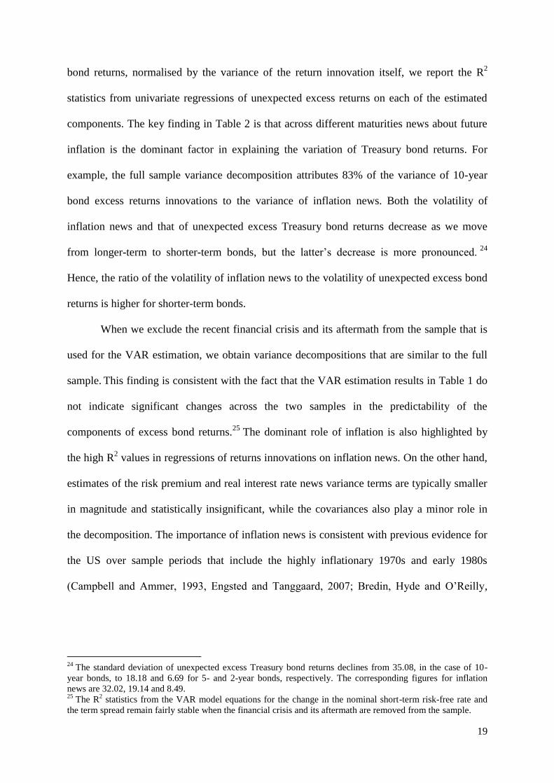
19

bond returns, normalised by the variance of the return innovation itself, we report the R2

statistics from univariate regressions of unexpected excess returns on each of the estimated

components. The key finding in Table 2 is that across different maturities news about future

inflation is the dominant factor in explaining the variation of Treasury bond returns. For

example, the full sample variance decomposition attributes 83% of the variance of 10-year

bond excess returns innovations to the variance of inflation news. Both the volatility of

inflation news and that of unexpected excess Treasury bond returns decrease as we move

from longer-term to shorter-term bonds, but the latter’s decrease is more pronounced. 24

Hence, the ratio of the volatility of inflation news to the volatility of unexpected excess bond

returns is higher for shorter-term bonds.

When we exclude the recent financial crisis and its aftermath from the sample that is

used for the VAR estimation, we obtain variance decompositions that are similar to the full

sample. This finding is consistent with the fact that the VAR estimation results in Table 1 do

not indicate significant changes across the two samples in the predictability of the

components of excess bond returns.25

The dominant role of inflation is also highlighted by

the high R2 values in regressions of returns innovations on inflation news. On the other hand,

estimates of the risk premium and real interest rate news variance terms are typically smaller

in magnitude and statistically insignificant, while the covariances also play a minor role in

the decomposition. The importance of inflation news is consistent with previous evidence for

the US over sample periods that include the highly inflationary 1970s and early 1980s

(Campbell and Ammer, 1993, Engsted and Tanggaard, 2007; Bredin, Hyde and O’Reilly,

24

The standard deviation of unexpected excess Treasury bond returns declines from 35.08, in the case of 10-

year bonds, to 18.18 and 6.69 for 5- and 2-year bonds, respectively. The corresponding figures for inflation

news are 32.02, 19.14 and 8.49. 25

The R2 statistics from the VAR model equations for the change in the nominal short-term risk-free rate and

the term spread remain fairly stable when the financial crisis and its aftermath are removed from the sample.

20

2010). 26

Thus, revisions in inflation expectations maintained their dominant influence over

the Treasury bond market during the era of lower inflation that commenced in the mid-1980s.

[TABLE 2 HERE]

4.3 Monetary policy effects on unexpected excess returns and their components

Tables 3-6 report estimates of the impact of monetary policy actions on unexpected

excess Treasury bond returns and their components over the full and pre-crisis sample

periods. 27

The results in Tables 3 and 4 are based on interest rate measures of monetary

policy (actual and unexpected change in the FFR, respectively). The first main finding from

interest rate measures is that monetary policy actions significantly affect the bond market

across all three maturities and across both sample periods. Monetary easing (FFR cuts) is

associated with higher contemporaneous unexpected excess returns. The second main result

is that the effect of monetary policy actions on the bond market is largely explained through

the inflation news channel. Specifically, we find that the key driver of the positive bond

returns’ response to FFR cuts is their negative effect on inflation expectations. 28

Another

feature of our results is the tendency of the FFR impact on bond returns and their main

26

In line with our results, Duffee’s (2014) findings using the Campbell and Ammer (1993) approach also

highlight the significant role of inflation news for the variance decomposition of 10-year bonds over a sample

period that commences during the Great Moderation and ends after the financial crisis (1987-2013). 27

Note that the VAR model that generates excess bond returns innovations and the associated news components

is estimated over the full sample period. The use of a longer sample should improve the precision of the

estimates. Nevertheless, we have also experimented by estimating pre-crisis monetary policy actions regressions

using returns innovations and news components extracted from a VAR model estimated with pre-crisis data.

Doing so, we find similar results to those reported in Tables 3-6. These results are available upon request. 28

Financial market participants tend to interpret expansionary monetary policy as a signal of worsening

economic outlook and thereby good news for Treasuries; see, for example, the following excerpt from the

Financial Times (2/2/2001): “Government bond prices rose yesterday as markets around the world digested

Wednesday’s 50 basis points interest rate cut by the US Federal Reserve. … slower growth and less inflation

was good for the bond market...”. All the more so, when monetary easing takes place during periods of

financial turmoil since it may reinforce flight to safety trading and therefore increase the price of Treasuries

(Kontonikas, MacDonald and Saggu; Goyenko and Ukhov, 2009).

21

component, inflation news, to increase in magnitude, albeit not monotonically, as the

maturity increases. 29

While reductions in the FFR exert a large and statistically significant effect on

inflation expectations, the impact on expected excess bond returns (term premium) is

typically smaller or insignificant. In the case of 10-year bonds the risk premium news

response is significant at the 5% level but the sign that it exhibits is different across the two

interest rate measures that we use. Using actual FFR changes, the positive effect of monetary

easing on expected excess returns is outweighed by the negative effect on inflation

expectations, so that the total effect on bond returns is positive.30

Finally, the response of

revisions in real interest rate expectations to FFR changes is almost always statistically

insignificant.

[TABLES 3-6 HERE]

Tables 5 and 6 use policy indicators that are related to the (log) monetary base (actual

and unexpected change, respectively). We focus on the full sample estimation results since

the pre-crisis sample excludes the recent financial crisis and its aftermath, that is, the period

when quantity-based indicators became strongly active due to the non-conventional policies

that were adopted by the Fed. The main insights that we identified using interest rate-based

measures remain overall valid in full sample estimations with quantity-based measures.

Particularly, the positive effect of monetary easing (higher monetary base growth) on

unexpected excess Treasury bond returns comes through downward revisions in inflation

29

Generally, event studies (Kuttner, 2001; Gurkaynak, Sack, and Swanson, 2005) and VAR studies (Berument

and Froyen, 2009) that analyse bond yields across the term structure find that the monetary policy impact

declines for longer maturities. Our approach, instead, considers unexpected excess bond returns. There are

various possible explanations for the significant reaction at the long-end of the bond market. Rolley and Sellon

(1995) point out that if policy actions are seen as relatively permanent or as the first in a series of future actions,

the response of long-term rates may be larger than the response of short-term rates. Over-reaction of long-term

rates to changes in short rates could also provide a mechanism to explain the impact of monetary policy

throughout the term structure (Romer and Romer, 2000). Finally, Ang et al. (2011) emphasise the role of shifts

in the Fed’s policy reaction function. 30

Re-arranging the dynamic identity shown in Equation (12), we can see that the total monetary policy effect on

unexpected excess bond returns must equal the negative sum of the effects on inflation, real interest rate and risk

premium news.

22

expectations, with the impact being generally stronger at longer maturities. The full sample

results indicate that money growth significantly affects real interest rate expectations,

whereas the impact on risk premium news tends to be statistically significant only when we

use actual changes in the (log) monetary base. The positive effect of monetary easing on

expected excess returns and real interest rates is compensated by the negative impact on

inflation expectations.

[FIGURES 3, 4 HERE]

Comparing the full sample with the pre-crisis results from quantity-based measures of

monetary policy, it becomes apparent that the former largely reflect developments that

occurred during the financial crisis. Following the collapse of Lehman Brothers in September

2008, inflation expectations sharply deteriorated in line with the worsening economic outlook

(Campbell, Shiller and Viceira, 2009). 31

At the same time, the Fed significantly expanded the

pace of monetary easing, both in the conventional and non-conventional sense. The FFR

declined by 160 basis points between September-November 2008 and the monetary base

growth rate recorded historical highs due to the heavy usage of non-sterilised Fed liquidity

facilities. Figures 3 and 4, which plot recursive estimates of the impact of actual and

unexpected (log) monetary base changes on unexpected excess Treasury bond returns and

inflation news, also suggest that an important structural shift took place in autumn 2008.

Following the unprecedented expansion in the monetary base and the announcement of QE1,

the relationship between money growth and bond returns tends to increase in magnitude,

while the impact on inflation expectations becomes strongly negative. The response

parameters exhibit a tendency to become smaller in size after the initial shock, suggesting

that further rounds of QE may not have been as influential as the first one.

31

By the autumn of 2008, inflation became strongly negative recording a sample minimum of -1.8% (month-on

month) in November 2008. The nominal short-term interest rate fell to almost zero, thereby pushing up the ex

post real interest rate to highly positive values.

23

Summarising our main results, we find that the positive effect of monetary easing on

the Treasury bond market is principally due to falls in inflation expectations. Moreover, our

results are overall not supportive of the portfolio balance mechanism, according to which

monetary easing, via an expansion of the Fed’s balance sheet, should increase current period

bond returns primarily through downward adjustments in expected excess returns (term

premium).

5. Robustness checks

We examine the robustness of our empirical findings in a number of ways and find

that the results reported in Section 4 are overall not sensitive to these changes. First, we

estimate monetary policy effects over an alternative sample period. Second, we use

alternative state vector specifications for the underlying VAR model. Third, we employ an

alternative interest rate-based policy indicator that accounts for Fed’s private information.

Fourth, we consider higher-order VARs. Fifth, we modify the model that is used to extract

monetary base growth surprises. Finally, we consider alternative quantity-based monetary

policy indicators. The results are contained in the Online Appendix C.

5.1 Alternative sample period

In the early 1990s, the Fed’s decisions to cut rates may have reflected an endogenous

reaction to labour market conditions. Between June 1989 and September 1992 (the date of the

last FFR cut associated with employment news), nearly half of the FOMC meetings coincided

with the release of a worse-than-expected employment report (Bernanke and Kuttner, 2005).

In this section, we examine the sensitivity of our findings regarding conventional monetary

policy actions to the exclusion of the pre-October 1992 period. The results are presented in

Tables C4 and C5 of the Online Appendix. With respect to 2-year bonds, they are

24

qualitatively similar to the main findings, with the positive effect of monetary easing on bond

returns being primarily explained by downward revisions in inflation expectations.

Nevertheless, the magnitude of the related coefficients is reduced. Meanwhile, the results for

5- and 10-year bonds are sensitive to the exclusion of the pre-October 1992 period.

Specifically, evidence for a significant bond market reaction to monetary policy shifts,

explained through the inflation news channel, becomes overall weaker.32

We also experimented with an alternative sample period commencing in February

1994, when the Fed started to announce target FFR changes and reduced substantially the

number of intermeeting policy rate changes. The results (available upon request) for 5- and

10-year bonds deteriorate further, while in the case of 2-year bonds they remain broadly

similar. The weaker bond market reaction to FFR shifts over the more recent period may be

related to changes in the way that the Fed implements and communicates monetary policy

(Fawley and Neely, 2014). These changes have enhanced transparency and enabled financial

markets to form more accurate expectations regarding the policy rate, leading to overall

smaller and less volatile target rate surprises over time.

5.2 Alternative state vector specifications

The benchmark VAR state vector includes the change in the nominal short-term risk-

free rate, the term spread, the real interest rate, and the relative bill rate. In addition to interest

rate variables, some studies find that macroeconomic factors and financial conditions

indicators and are helpful in predicting bond returns (Ang and Piazzesi, 2003; Ludvigson and

Ng, 2009; Fricke and Menkhoff, 2014). Motivated by this evidence, we examine whether our

baseline findings are robust to incorporating measures of macro-financial conditions in the

VAR state vector. The following variables are considered: industrial production growth rate,

32

The puzzling full sample finding of a positive and statistically significant response of 10-year bonds returns to

tightening surprises is driven by crisis period developments.

25

unemployment, the Chicago Fed National Activity Index (CFNAI), and the Chicago Fed

Adjusted National Financial Conditions Index (ANFCI). 33

CFNAI is a measure of overall

economic activity, calculated as the weighted average of 85 monthly indicators of national

economic activity. ANFCI isolates the component of financial conditions (in money markets,

debt and equity markets, and the traditional and “shadow” banking systems) that is

uncorrelated with economic conditions.

The variance decomposition results that we obtain using the alternative state vectors

are shown in shown in Tables C6-C9 in Appendix C, while the corresponding monetary

policy effects regressions are presented in Tables C10-C25. Overall, as in the case of the

benchmark state vector variance decomposition, inflation news is the major component of

unexpected excess Treasury bond returns. Furthermore, as in the baseline results, the positive

effect of monetary easing on bond returns comes from a corresponding negative effect on

inflation expectations. Thus, accounting for additional forecasting variables does not alter the

conclusions from the baseline analysis.

5.3 Alternative interest rate-based policy measure

If policy actions reveal private information held by the central bank about the future

state of the economy, estimates of monetary policy effects on economic and financial

variables may be biased. Romer and Romer (2004) propose an alternative way to identify

monetary policy shocks that takes into account the central bank’s response to expected

economic conditions.34

The results presented in Table C26 use Romer and Romer’s shocks.

33

Both CFNAI and ANFCI may provide useful information about current and future developments in economic

and financial conditions. More details about these indices can be found at:

https://www.chicagofed.org/publications/cfnai/index and https://www.chicagofed.org/publications/nfci/index. 34

The calculation of Romer and Romer’s (2004) monetary policy shocks involves two steps. First, intended

federal funds rate changes around the FOMC meetings are identified. Second, the intended funds rate changes

are regressed on the internal FOMC forecasts for inflation and real economic activity, i.e. the Greenbook

forecasts, around the dates of these forecasts; see Equation (1) in Romer and Romer (2004). Residuals from that

regression represent monetary policy shocks. To obtain these shocks, we used the STATA code provided by

Wieland and Yang (2015).

26

The conclusions that we draw are similar to those from the baseline findings in Tables 3 and

4, since bond returns respond positively to monetary easing and inflation expectations play a

key role in explaining this reaction.

5.4 Higher order VARs

The benchmark VAR model is first-order VAR. In order to examine whether a more

complex dynamic structure affects the baseline results, we consider higher order VARs (Barr

and Pesaran, 1997; Maio, 2014). The variance decomposition and monetary policy effects

results in Tables C27 and C28-C31, respectively, in Appendix C are based upon a third-order

VAR model. They indicate that the main conclusions about the role of inflation news in the

variance decomposition, as well as the relationship between bond returns and monetary

policy, and are not affected by parsimony in the VAR order. Similar insights are provided by

VAR(2) and VAR(6) models. These results are available upon request.

5.5 Alternative models for monetary base growth surprises

The monetary base growth surprises that we use in the baseline analysis are obtained

as residuals from a regression of monetary base growth on its own lags and lags of

unemployment. Following previous work by Cover (1992), we model monetary base growth

using two additional specifications for the set of explanatory variables. Specifically, lags of

monetary base growth are complemented with either lags of industrial production growth, or

lags of industrial production growth and lags of the first difference of the 3-monthTreasury

bill rate. Estimates of monetary policy effects using these alternative measures of monetary

base growth surprises are presented in Tables C32 and C33 in Appendix C. They are overall

similar to the benchmark results. The positive bond market response to monetary easing is

mainly explained by downward revisions in inflation expectations.

27

5.6 Alternative quantity-based monetary policy indicator

The large increase in total reserves, commencing at the end of 2008, made them the

dominant component of the monetary base. Motivated by this development, we consider two

additional quantity-based measures of monetary policy: actual and unexpected changes in

(log) total reserves. As with monetary base growth surprises, the latter are obtained as

residuals from a regression of total reserves growth on their own lags and lags of

unemployment. The results from monetary policy regressions with total reserves as a

quantity-based indicator are shown in Tables C34 and C35 in Appendix C. The main

conclusions from the baseline analysis remain valid since monetary policy shifts have a

significant effect on bond market performance and inflation news is typically the main

component of bond returns that is affected.

6. Conclusions

Following the recent financial crisis and the actions taken by the Fed, analyses of the

sources of variation in the bond market and the role of monetary policy came to the focus of

academics, investors and policymakers. This paper extends the analysis of Campbell and

Ammer (1993) to investigate the sources of variation in Treasury bond returns across

different maturities. This framework combines a dynamic accounting identity with a VAR

time-series econometric model to decompose unexpected excess bond returns into revisions

in expectations (news) about future excess returns, inflation and real interest rates.

Furthermore, we modify Bernanke and Kuttner’s (2005) extension of Campbell and Ammer’s

framework to obtain insights to the sources of the bond market’s response to monetary

policy. Using this approach, we estimate the impact of actual and unexpected changes in

monetary policy indicators on bond returns and their components. We use FFR-based

indicators to capture conventional monetary policy, whereas shifts in the monetary base are

28

employed to capture the non-conventional dimensions of monetary policy during the crisis

and its aftermath.

The variance decomposition results show that news about future inflation constitute

the largest component of unexpected excess Treasury bond returns, while the contribution of

risk premium news and real interest rate news is typically negligible. Hence, we confirm and

update previous empirical evidence about the importance of inflation news for longer-term

bonds by showing that they maintained their dominant influence during the era of lower

inflation that commenced in the mid-1980s. Moreover, we complete the picture by providing

new evidence which shows that inflation news also dominate the variance decomposition of

medium- and shorter-term bonds.

With respect to the impact of monetary policy actions, the results generally indicate

that monetary easing is associated with higher bond returns. Nevertheless, the effect of

interest rate-based policy measures on bond returns has become weaker over the more recent

period possibly reflecting changes, ever since the mid-1990s, in the way that the Fed

implements and communicates monetary policy. In the case of quantity-based monetary

policy indicators, the bond market response largely reflects developments that occurred at the

peak of the financial crisis in autumn 2008. As to why the bond market responds in this

manner, the results highlight the role of inflation news. We find that the positive effect of

monetary easing on bond returns mainly comes from a corresponding negative effect on

inflation expectations. On the other hand, evidence in favour of the portfolio balance

mechanism’s prediction of a strong role for risk premium news within the context of an

expanding Fed balance sheet is rather elusive.

29

References

Ang, A., Boivin, J., Dong, S., and Loo-Kung, R., 2011. Monetary policy shifts and the term

structure. Review of Economic Studies, 78(2), p.429-457.

Ang, A., and Piazzesi, M., 2003. A no-arbitrage vector autoregression of term structure

dynamics with macroeconomic and latent variables. Journal of Monetary Economics,

50(4), p.745-787.

Balke, N.S., and Emery, K.M., 1994. Understanding the price puzzle. Federal Reserve Bank

of Dallas Economic Review, 4, p.15-26.

Barakchian, S.M., and Crowe, C., 2013. Monetary policy matters: evidence from new shocks

data. Journal of Monetary Economics, 60(8), p.950-966.

Barr, D., and Pesaran, B., 1997. An assessment of the relative importance of real interest

rates, inflation, and term premiums in determining the prices of real and nominal U.K.

bonds. Review of Economics and Statistics, 79(3), p.362-366.

Bauer, M.D., and Rudebusch, G.D., 2013. The signaling channel for Federal Reserve bond

purchases. Federal Reserve Bank of San Francisco Working Paper Series, Working

paper 2011-21.

Bernanke, B.S., and Blinder, A.S., 1992. The Federal funds rate and the channels of monetary

transmission. American Economic Review, 82(4), p.901-921.

Bernanke, B.S., and Kuttner, B.N., 2005. What explains the stock market’s reaction to

Federal Reserve policy? Journal of Finance, 60(3), p.1221-1257.

Bernanke and Mihov, 1998. Measuring monetary policy. Quarterly Journal of Economics,

113(3), p.869-902.

Berument, H., and Froyen, R., 2009. Monetary policy and U.S. long-term interest rates: How

close are the linkages? Journal of Economics and Business, 61, p.34-50.

30

Bredin, D., Hyde, S., and O’Reilly, G., 2010. Monetary policy surprises and international

bond markets. Journal of International Money and Finance, 29(6), p.988-1002.

Brunnermeier, M.K., 2009. Deciphering the liquidity and credit crunch 2007-2008. Journal of

Economic Perspectives, 23(1), p.77-100.

Campbell, J.Y., 1991. A variance decomposition for stock returns. Economic Journal,

101(405), p.157-179.

Campbell, J. Y., and Ammer, J., 1993. What moves the stock and bond markets? A variance

decomposition for long term asset returns. Journal of Finance, 48(1), p.3-37.

Campbell, J.Y., Lo, A.W., and MacKinlay, A.C., 1997. The econometrics of financial

markets. New Jersey: Princeton University Press.

Campbell, J.Y., and Shiller, R.J., 1988. The dividend–price ratio and expectations of future

dividends and discount factors. Review of Financial Studies, 1(3), p.195-228.

Campbell, J.Y., and Shiller, R.J., 1991.Yield spreads and interest rate movements: A bird’s

eye view. Review of Economic Studies, 58(3), p.495-514.

Campbell, J.Y., Shiller, R.J., and Viceira, L.M., 2009. Understanding inflation-indexed bond

markets. NBER Working Paper Series, Working paper 15014.

Cenedese, G., and Mallucci, E., 2015. What moves international stock and bond markets?

Journal of International Money and Finance, forthcoming.

Chen, S., 2007. Does monetary policy have asymmetric effects on stock returns? Journal of

Money, Credit and Banking, 39(2-3), p.667-688.

Chen, L., and Zhao, X., 2009. Return decomposition. Review of Financial Studies, 22(12),

p.5213-5246.

Chernov, M, and Mueller, P., 2012. The term structure of inflation expectations. Journal of

Financial Economics, 106(2), p.367-394.

31

Christensen, J.H.E., and Rudebusch, G.D., 2012. The response of interest rates to US and UK

quantitative easing. Economic Journal, 122(564), p.385-414.

Christopoulos, D.K., and Leon-Ledesma, M.A., 2007. A long-run non-linear approach to the

Fisher effect. Journal of Money, Credit, and Banking, 39(2-3), p.543-559.

Cochrane, J.H., and Piazzesi, M., 2002. The Fed and interest rates: A high-frequency

identification. American Economic Review Papers and Proceedings, 92(2), 90-95.

Cover, J.P., 1992. Asymmetric effects of positive and negative money-supply shocks.

Quarterly Journal of Economics, 107(4), p.1261-1282.

Curdia, V., and Woodford, M., 2011. The central-bank balance sheet as an instrument of

monetary policy. Journal of Monetary Economics, 58(1), p.54-79.

D'Amico, S., English, W., Lopez-Salido, D., and Nelson, E., 2012. The Federal Reserve's

large-scale asset purchase programmes: rationale and effects. Economic Journal,

122(564), p.415-446.

Duffee, G.R., 2014. Expected inflation and other determinants of Treasury yields. Johns

Hopkins University, Working paper.

Engsted, T., Pedersen, T.Q., and Tanggaard, C., 2012. Pitfalls in VAR based return

decompositions: a clarification. Journal of Banking and Finance, 36(5), p.1255-1265.

Engsted, T., and Tanggaard, C., 2007. The comovement of U.S. and German bond markets.

International Review of Financial Analysis, 16(2), p.172-182.

Evans, C.L., and Kuttner, K.N., 1998. Can VARs describe monetary policy? Federal Reserve

Bank of Chicago Working Paper Series, Working paper 98-19.

Fama, E.F., 2013. Does the Fed control interest rates? Review of Asset Pricing Studies, 3(2),

p.180-199.

Fama, E.F, and Bliss, R., 1987. The information in long-maturity forward rates. American

Economic Review, 77(4), p. 680-692

32

Faust, J., Swanson, E.T., and Wright, J.H., 2004. Do Federal Reserve policy surprises reveal

superior information about the economy? Contributions to Macroeconomics, 4(1),

p.1-31.

Fawley, B.W., and Neely, C.J., 2013. Four stories of quantitative easing. Federal Reserve

Bank of St. Louis Review, 95(1), p.51-88.

Fawley, B.W., and Neely, C.J., 2014. The evolution of Federal Reserve policy and the impact

of monetary policy surprises on asset prices. Federal Reserve Bank of St. Louis

Review, 96(1), p.73-109.

Fricke, C., and Menkhoff, L., 2014. Financial conditions, macroeconomic factors and

(un)expected bond excess returns. Deutsche Bundesbank, discussion paper 35/2014.

Gagnon, J., Raskin, M., Remache, J., and Sack, B., 2011. Large-scale asset purchases by the

Federal Reserve: did they work? Federal Reserve Bank of New York Economic Policy

Review, 17(1), p.41-59.

Gambacorta, L., Hofmann, B., and Peersman, G., 2014. The effectiveness of unconventional

monetary policy at the zero lower bound: a cross-country analysis. Journal of Money,

Credit and Banking, 46(4), p.615-642.

Gertler, M., and Karadi, P., 2013. QE 1 vs. 2 vs. 3. . . : A Framework for analyzing large-scale

asset purchases as a monetary policy tool. International Journal of Central Banking,

9(1), p.5-53.

Gertler, M., and Karadi, P., 2015. Monetary policy surprises, credit costs, and economic

activity. American Economic Journal: Macroeconomics, 7(1), p.44-76.

Goyenko, R.Y., and Ukhov, A.D., 2009. Stock and bond market liquidity: a long-run

empirical analysis. Journal of Financial and Quantitative Analysis, 44(1), p.189-212.

Greenwood, R., and Vayanos, D., 2014. Bond supply and excess bond returns. Review of

Financial Studies, 27(3), p.663-713.

33

Gurkaynak, R.S., Sack, B., and Swanson, E.T., 2005. Do actions speak louder than words?

The response of asset prices to monetary policy actions and statements. International

Journal of Central Banking, 1(1), p.55-93.

Gurkaynak, R.S., Sack, B., and Wright, J.H., 2007. The U.S. treasury yield curve: 1961 to the

present. Federal Reserve Board Finance and Economics Discussion Series, Working

paper 2006-28.

Harada, Y., and Masujima, M., 2009. Japanese Economy, 36(1), p.48-105.

Karras, G., 2013. Asymmetric effects of monetary policy with or without quantitative easing:

empirical evidence for the US. Journal of Economic Asymmetries, 10(1), p.1-9.

Kimura, T., Kobayashi, H., Muranaga, J., and Ugai, H., 2003. The effect of the increase in the

monetary base on Japan’s economy at zero interest rates: an empirical analysis. Bank

for International Settlements, Working paper 19.

Kontonikas, A., and Kostakis, A., 2013. On monetary policy and stock market anomalies.

Journal of Business Finance and Accounting, 40(7-8), p.1009-1042.

Kontonikas, A., MacDonald, R., and Saggu, A. (2013). Stock market reaction to Fed funds

rate surprises: state dependence and the financial crisis. Journal of Banking and

Finance, 37(11), p.4025-4037.

Kuttner, K.N., 2001. Monetary policy surprises and interest rates: evidence from the fed

funds futures market. Journal of Monetary Economics, 47(3), p.523-544.

Ludvigson, S.C., and Ng, S., 2009. Macro factors in bond risk premia. Review of Financial

Studies, 22(12), p.5027-5067.

Maio, P., 2014. Another look at the stock return response to monetary policy actions. Review

of Finance, 18(1), p.321-371.

Nimark, K., 2008. Monetary policy with signal extraction from the bond market. Journal of

Monetary Economics, 55(8), p.1389-1400.

34

Ostrovsky, A., Rahman, B., and Rayner, A., 2001. Treasuries lifted by Fed rate cut. Financial

Times 2 February, 2001, p.36.

Piazzesi, M., and Schneider, M., 2007. Equilibrium yield curves. In: Acemoglu, D., Rogoff,

K., and Woodford, M. eds. NBER Macroeconomics Annual 2006. Cambridge: The

MIT Press, p.389-472.

Rigobon, R., and Sack, B., 2004. The impact of monetary policy on asset prices. Journal of

Monetary Economics, 51(8), p.1553-1575.

Rolley, V.V., and Sellon, G.H.Jr., 1995. Monetary policy actions and long-term interest rates.

Federal Reserve Bank of Kansas City Economic Review, 80(4), p.77-89.

Romer, C.D., and Romer, D.H., 2000. Federal Reserve information and the behavior of

interest rates. American Economic Review, 90(3), p.429-457.

Romer, C.D., and Romer, D.H., 2004. A new measure of monetary shocks: Derivation and

implications. American Economic Review, 94(4), p.1055-1084.

Sarno, L., Thornton, D.L., and Valente, G., 2007. The empirical failure of the expectations

hypothesis of the term structure of bond yields. Journal of Financial and Quantitative

Analysis, 42(1), p.81-100.

Thornton, D.L., 2005. Tests of the expectations hypothesis: resolving the anomalies when the

short-term rate is the Federal funds rate. Journal of Banking and Finance, 29(10),

p.2541-2556.

Thornton, D.L., 2012. Evidence on the portfolio balance channel of quantitative easing.

Federal Reserve Bank of St. Louis Working Paper Series, Working paper 2012-015A.

Thornton, D.L., 2013. The identification of the response of interest rates to monetary policy

actions using market-based measures of monetary policy shocks. Oxford Economic

Papers, 66(1), p.67-87.

35

Vayanos, D., and Vila, J-L., 2009. A preferred-habitat model of the term structure of interest

rates. NBER Working Paper Series, Working paper 15487.

Vazquez, J., Maria-Dolores, R., and Londono, J., 2013. On the informational role of term

structure in the US monetary policy rule. Journal of Economic Dynamics and Control,

37(9), p.1852-1871.

Wieland, J.F., and Yang, M., 2015. Financial dampening. Working paper.

36

Figure 1: Policy rate and monetary aggregates

Notes: This figure plots the target Federal funds rate (FFR target), the St. Louis adjusted total reserves (in $bn),

the M2 money stock (in $bn) and the St. Louis adjusted monetary base (in $bn) over the full sample period

(1985:1 – 2014:2). The dashed vertical line in the upper left panel denotes the start of zero lower bound period.

In the rest of the panels, the three dashed vertical lines denote the announcements of first round of quantitative

easing (QE1, 2008:11), second round (QE2, 2010:11) and third round (QE3, 2012:9). Shaded areas denote US

recessions as classified by NBER business cycle dates. Data is obtained from the FREDII database.

0

2

4

6

8

10

1985 1990 1995 2000 2005 2010

FFR target

0

500

1,000

1,500

2,000

2,500

3,000

1985 1990 1995 2000 2005 2010

Total Reserves

2,000

4,000

6,000

8,000

10,000

12,000

1985 1990 1995 2000 2005 2010

M2

0

1,000

2,000

3,000

4,000

5,000

1985 1990 1995 2000 2005 2010

Monetary Base

QE1

QE2

QE3

ZLB

37

Figure 2: Monetary policy indicators

Notes: This figure plots our four monetary policy actions indicators over the full sample period (1985:1 –

2014:2); the change in the Federal funds rate (FFR), the unexpected FFR change, the change in log monetary

base (MB change) and the unexpected change in log monetary base. For further details, see Section 3.3. Shaded

areas denote US recessions as classified by NBER business cycle dates.

-1.0

-0.5

0.0

0.5

1.0

1985 1990 1995 2000 2005 2010

FFR change

-.8

-.6

-.4

-.2

.0

.2

.4

1985 1990 1995 2000 2005 2010

Unexpected FFR change

-10

0

10

20

30

1985 1990 1995 2000 2005 2010

MB change

-10

-5

0

5

10

15

1985 1990 1995 2000 2005 2010

Unexpected MB change

38

Figure 3: Recursive estimates of MB change impact

Panel A: 10-year bonds

Panel B: 5-year bonds

Panel C: 2-year bonds

Notes: This figure plots recursive estimates of the response parameters of unexpected excess Treasury bond

returns and the corresponding inflation news component to actual changes in log monetary base (MB). Panel A

refers to 10-year bonds, Panel B to 5-year bonds and Panel C to 2-year bonds. The initial sample of the recursive

estimation is 1985:1 – 1995:1 and then one month is added at each step. The shaded area denotes the period of

quantitative easing, starting from the announcement of QE1 (2008:11).

-4

-3

-2

-1

0

1

2

2004 2005 2006 2007 2008 2009 2010 2011 2012 2013

Response of unexpected excess returns: 10-year bonds

-4

-3

-2

-1

0

1

2

3

2004 2005 2006 2007 2008 2009 2010 2011 2012 2013

Response of revisions in inlfation expectations

0.2

0.4

0.6

0.8

1.0

1.2

1.4

2004 2005 2006 2007 2008 2009 2010 2011 2012 2013

Response of unexpected excess returns: 5-year bonds

-2.5

-2.0

-1.5

-1.0

-0.5

0.0

0.5

2004 2005 2006 2007 2008 2009 2010 2011 2012 2013

Response of revisions in inflation expectations

.32

.36

.40

.44

.48

.52

.56

.60

.64

.68

2004 2005 2006 2007 2008 2009 2010 2011 2012 2013

Response of unexpected excess returns: 2-year bonds

-1.6

-1.2

-0.8

-0.4

0.0

0.4

2004 2005 2006 2007 2008 2009 2010 2011 2012 2013

Response of revisions in inflation expectations

Quantitative Easing Quantitative Easing

Quantitative Easing Quantitative Easing

Quantitative Easing Quantitative Easing

-4

-3

-2

-1

0

1

2

2004 2005 2006 2007 2008 2009 2010 2011 2012 2013

Response of unexpected excess returns: 10-year bonds

-4

-3

-2

-1

0

1

2

3

2004 2005 2006 2007 2008 2009 2010 2011 2012 2013

Response of revisions in inlfation expectations

0.2

0.4

0.6

0.8

1.0

1.2

1.4

2004 2005 2006 2007 2008 2009 2010 2011 2012 2013

Response of unexpected excess returns: 5-year bonds

-2.5

-2.0

-1.5

-1.0

-0.5

0.0

0.5

2004 2005 2006 2007 2008 2009 2010 2011 2012 2013

Response of revisions in inflation expectations

.32

.36

.40

.44

.48

.52

.56

.60

.64

.68

2004 2005 2006 2007 2008 2009 2010 2011 2012 2013

Response of unexpected excess returns: 2-year bonds

-1.6

-1.2

-0.8

-0.4

0.0

0.4

2004 2005 2006 2007 2008 2009 2010 2011 2012 2013

Response of revisions in inflation expectations

Quantitative Easing Quantitative Easing

Quantitative Easing Quantitative Easing

Quantitative Easing Quantitative Easing

-4

-3

-2

-1

0

1

2

2004 2005 2006 2007 2008 2009 2010 2011 2012 2013

Response of unexpected excess returns: 10-year bonds

-4

-3

-2

-1

0

1

2

3

2004 2005 2006 2007 2008 2009 2010 2011 2012 2013

Response of revisions in inlfation expectations

0.2

0.4

0.6

0.8

1.0

1.2

1.4

2004 2005 2006 2007 2008 2009 2010 2011 2012 2013

Response of unexpected excess returns: 5-year bonds

-2.5

-2.0

-1.5

-1.0

-0.5

0.0

0.5

2004 2005 2006 2007 2008 2009 2010 2011 2012 2013

Response of revisions in inflation expectations

.32

.36

.40

.44

.48

.52

.56

.60

.64

.68

2004 2005 2006 2007 2008 2009 2010 2011 2012 2013

Response of unexpected excess returns: 2-year bonds

-1.6

-1.2

-0.8

-0.4

0.0

0.4

2004 2005 2006 2007 2008 2009 2010 2011 2012 2013

Response of revisions in inflation expectations

Quantitative Easing Quantitative Easing

Quantitative Easing Quantitative Easing

Quantitative Easing Quantitative Easing

39

Figure 4: Recursive estimates of unexpected MB change impact

Panel A: 10-year bonds

Panel B: 5-year bonds

Panel C: 2-year bonds

Notes: This figure plots recursive estimates of the response parameters of unexpected excess Treasury bond

returns and the corresponding inflation news component to unexpected changes in log monetary base. See also

Figure 3 notes.

-3

-2

-1

0

1

2

2004 2005 2006 2007 2008 2009 2010 2011 2012 2013

Response of unexpected excess returns: 10-year bonds

-4

-3

-2

-1

0

1

2

3

2004 2005 2006 2007 2008 2009 2010 2011 2012 2013

Response of revisions in inflation expectations

0.6

0.8

1.0

1.2

1.4

1.6

1.8

2004 2005 2006 2007 2008 2009 2010 2011 2012 2013

Response of unexpected excess returns: 5-year bonds

-2.8

-2.4

-2.0

-1.6

-1.2

-0.8

-0.4

0.0

0.4

0.8

2004 2005 2006 2007 2008 2009 2010 2011 2012 2013

Response of revisions in inflation expectations

.1

.2

.3

.4

.5

.6

.7

.8

2004 2005 2006 2007 2008 2009 2010 2011 2012 2013

Response of unexpected excess returns: 2-year bonds

-2.0

-1.6

-1.2

-0.8

-0.4

0.0

0.4

0.8

2004 2005 2006 2007 2008 2009 2010 2011 2012 2013

Response of revisions in inflation expectations

Quantitative Easing Quantitative Easing

Quantitative Easing Quantitative Easing

Quantitative Easing Quantitative Easing

-3

-2

-1

0

1

2

2004 2005 2006 2007 2008 2009 2010 2011 2012 2013

Response of unexpected excess returns: 10-year bonds

-4

-3

-2

-1

0

1

2

3

2004 2005 2006 2007 2008 2009 2010 2011 2012 2013

Response of revisions in inflation expectations

0.6

0.8

1.0

1.2

1.4

1.6

1.8

2004 2005 2006 2007 2008 2009 2010 2011 2012 2013

Response of unexpected excess returns: 5-year bonds

-2.8

-2.4

-2.0

-1.6

-1.2

-0.8

-0.4

0.0

0.4

0.8

2004 2005 2006 2007 2008 2009 2010 2011 2012 2013

Response of revisions in inflation expectations

.1

.2

.3

.4

.5

.6

.7

.8

2004 2005 2006 2007 2008 2009 2010 2011 2012 2013

Response of unexpected excess returns: 2-year bonds

-2.0

-1.6

-1.2

-0.8

-0.4

0.0

0.4

0.8

2004 2005 2006 2007 2008 2009 2010 2011 2012 2013

Response of revisions in inflation expectations

Quantitative Easing Quantitative Easing

Quantitative Easing Quantitative Easing

Quantitative Easing Quantitative Easing

-3

-2

-1

0

1

2

2004 2005 2006 2007 2008 2009 2010 2011 2012 2013

Response of unexpected excess returns: 10-year bonds

-4

-3

-2

-1

0

1

2

3

2004 2005 2006 2007 2008 2009 2010 2011 2012 2013

Response of revisions in inflation expectations

0.6

0.8

1.0

1.2

1.4

1.6

1.8

2004 2005 2006 2007 2008 2009 2010 2011 2012 2013

Response of unexpected excess returns: 5-year bonds

-2.8

-2.4

-2.0

-1.6

-1.2

-0.8

-0.4

0.0

0.4

0.8

2004 2005 2006 2007 2008 2009 2010 2011 2012 2013

Response of revisions in inflation expectations

.1

.2

.3

.4

.5

.6

.7

.8

2004 2005 2006 2007 2008 2009 2010 2011 2012 2013

Response of unexpected excess returns: 2-year bonds

-2.0

-1.6

-1.2

-0.8

-0.4

0.0

0.4

0.8

2004 2005 2006 2007 2008 2009 2010 2011 2012 2013

Response of revisions in inflation expectations

Quantitative Easing Quantitative Easing

Quantitative Easing Quantitative Easing

Quantitative Easing Quantitative Easing

40

Table 1: VAR estimates

10-year bonds 5-year bonds 2-year bonds

1985:1 – 2014:2

1,ty ,n ts i

tr trb 2R 1,ty ,n ts i

tr trb 2R 1,ty ,n ts i

tr trb 2R

1, 1ty -0.425***

(0.072)

0.085***

(0.026)

-0.010

(0.007)

0.103**

(0.041) 0.196

-0.414***

(0.073)

0.148***

(0.032)

-0.011

(0.007)

0.110***

(0.038) 0.236

-0.359***

(0.073)

0.271***

(0.041)

-0.017***

(0.006)

0.067*

(0.035) 0.322

, 1n ts 0.431***

(0.078)

0.885***

(0.028)

-0.000

(0.009)

-0.129***

(0.047) 0.814

0.396***

(0.078)

0.834***

(0.035)

0.003

(0.008)

-0.107**

(0.045) 0.719

0.328***

(0.080)

0.754***

(0.046)

0.008

(0.007)

-0.031

(0.042) 0.557

1

i

tr 0.139

(0.284)

-0.366**

(0.150)

0.515***

(0.077)

-0.106

(0.217) 0.324

0.124

(0.282)

-0.215

(0.143)

0.545***

(0.070)

0.042

(0.220) 0.313

0.137

(0.283)

-0.018

(0.169)

0.557***

(0.068)

0.132

(0.219) 0.400

1trb -0.382***

(0.070)

0.096***

(0.026)

-0.010

(0.007)

0.974***

(0.039) 0.711

-0.369***

(0.071)

0.157***

(0.032)

-0.012**

(0.006)

0.978***

(0.037) 0.726

-0.315***

(0.071)

0.272***

(0.041)

-0.018***

(0.006)

0.931***

(0.033) 0.756

1985:1 – 2007:7

1, 1ty -0.443***

(0.075)

0.087***

(0.032)

-0.015

(0.012)

0.098**

(0.048) 0.215

-0.433***

(0.073)

0.148***

(0.032)

-0.013

(0.011)

0.112**

(0.045) 0.249

-0.374***

(0.076)

0.279***

(0.046)

-0.015

(0.010)

0.075*

(0.038) 0.334

, 1n ts 0.431***

(0.081)

0.886***

(0.036)

0.007

(0.015)

-0.121**

(0.055) 0.802

0.394***

(0.082)

0.830***

(0.043)

0.004

(0.014)

-0.110**

(0.054) 0.708

0.323***

(0.084)

0.736***

(0.053)

0.003

(0.012)

-0.038

(0.048) 0.523

1

i

tr 0.242

(0.265)

-0.488***

(0.140)

0.399***

(0.083)

-0.358*

(0.195) 0.266

0.204

(0.265)

-0.416***

(0.155)

0.434***

(0.081)

-0.215

(0.193) 0.250

0.157

(0.266)

-0.281

(0.183)

0.465***

(0.080)

-0.032

(0.194) 0.236

1trb -0.401***

(0.074)

0.098***

(0.032)

-0.015

(0.012)

0.971***

(0.046) 0.687

-0.390***

(0.075)

0.156***

(0.038)

-0.015

(0.011)

0.982***

(0.043) 0.700

-0.332***

(0.075)

0.278***

(0.046)

-0.017*

(0.010)

0.940***

(0.037) 0.733

Notes: This table reports the estimated parameters of the benchmark VAR(1) model shown in Equation (3) for 10-, 5- and 2-year bonds. The state vector contains the first

difference in 1-month Treasury bill rate (∆y1), the yield spread between 10-, 5- and 2-year Treasury bonds and the 1-month Treasury bill (sn), the real interest rate (ri) and

the relative bill rate (rb). All variables are expressed in percentages per annum on continuously compounded basis. The upper panel of the table provides the full sample

(1985:1 – 2014:2) estimates while the pre-crisis period (1985:1 – 2007:7) estimates are shown in the lower panel. Heteroskedasticity and autocorrelation-consistent

standard errors are shown in parentheses. ***, **, * denote 1%, 5% and 10% level of significance, respectively.

41

Table 2: Variance decomposition for excess bond returns

10-year bonds 5-year bonds 2-year bonds

1985:1–2014:2 1985:1–2007:7 1985:1–2014:2 1985:1–2007:7 1985:1–

2013:12 1985:1–2007:7

Var x 0.833***

(0.264)

0.799***

(0.243)

1.108**

(0.430)

1.116**

(0.447)

1.607**

(0.763)

1.675**

(0.700)

2 , irCov x x

-0.087

(0.083)

-0.085

(0.087)

-0.189

(0.189)

-0.225

(0.191)

-0.674

(0.698)

-0.673

(0.595)

2 , xCov x x 0.046

(0.285)

0.148

(0.200)

-0.098

(0.352)

0.015

(0.331)

-0.553

(0.448)

-0.314

(0.421)

irVar x 0.018*

(0.010)

0.017

(0.012)

0.038

(0.023)

0.035

(0.024)

0.266*

(0.147)

0.143

(0.111)

2 ,i xrCov x x -0.068

(0.056)

-0.102*

(0.058)

0.025

(0.067)

-0.052

(0.069)

0.252

(0.171)

0.081

(0.128)

xVar x 0.258

(0.168)

0.223

(0.177)

0.116

(0.101)

0.112

(0.109)

0.102

(0.074)

0.088

(0.070)

2R x 0.793***

(0.154)

0.863***

(0.140)

0.839***

(0.113)

0.915***

(0.083)

0.614***

(0.163)

0.834***

(0.102)

2ir

R x 0.199

(0.145)

0.334**

(0.152)

0.050

(0.133)

0.314

(0.202)

0.011

(0.087)

0.164

(0.252)

2

xR x 0.236

(0.202)

0.271

(0.203)

0.054

(0.221)

0.078

(0.268)

0.023

(0.149)

0.009

(0.103)

Notes: This table reports the variance decomposition of unexpected excess returns of 10-, 5-, and 2-year Treasury bonds into the variances of inflation news

( x ), real interest rate news ( irx ), risk premium news (

xx ) and the covariances between these three components. News components are extracted from a

VAR(1) model where the state vector contains the first difference in 1-month Treasury bill rate, the yield spread between 10-, 5- and 2-year Treasury bonds

and the 1-month Treasury bill, the real interest rate and the relative bill rate. The first and second column for each bond maturity report the full sample

(1985:1 – 2014:2) and pre-crisis period (1985:1 – 2007:7) results, respectively. R2 values are obtained from regressions of unexpected excess returns on

each news component. The standard errors reported in parentheses are computed using the delta method. ***, **, * denote 1%, 5% and 10% level of

significance, respectively..

42

Table 3: Impact of monetary policy on excess bond returns – FFR change

10-year bonds 5-year bonds 2-year bonds

FFR 1985:1 – 2014:2 1985:1 – 2007:7 1985:1 – 2014:2 1985:1 – 2007:7 1985:1 – 2014:2 1985:1 – 2007:7

MP

nx -20.88***

(4.662)

-20.44***

(4.411)

-15.59***

(2.969)

-13.84***

(2.801)

-8.51***

(1.349)

-7.87***

(1.305)

i

MP

rx

0.94

(1.829)

1.55

(1.663)

-1.51

(1.257)

-0.71

(1.078)

-2.09

(1.593)

-1.29

(1.374)

MPx 36.29***

(8.331)

32.90***

(7.532)

23.03***

(3.668)

19.67***

(3.332)

13.11***

(1.947)

11.19***

(1.661)

MP

xx -16.36**

(7.833)

-14.01**

(6.878)

-5.93*

(3.544)

-5.12

(3.089)

-2.51**

(1.265)

-2.03*

(1.126)

Notes: This table reports the impact of a change in the Federal funds rate (FFR) on the unexpected excess returns of

10-, 5-, and 2-year Treasury bonds (nx ), inflation news ( x ), real interest rate news ( ir

x ) and risk premium news (xx ).

News components are extracted from a VAR(1) model estimated over the full sample period (1985:1 – 2014:2). The

state vector contains the first difference in 1-month Treasury bill rate, the yield spread between 10-, 5- and 2-year

Treasury bonds and the 1-month Treasury bill, the real interest rate and the relative bill rate. The first and second

column for each bond maturity report the full sample and pre-crisis period (1985:1 – 2007:7) results, respectively. The

standard errors reported in parentheses are computed using the delta method. ***, **, * denote 1%, 5% and 10% level

of significance, respectively.

43

Table 4: Impact of monetary policy on excess bond returns – Unexpected FFR change

10-year bonds 5-year bonds 2-year bonds

UFFR 1989:2 – 2014:2 1989:2 – 2007:7 1989:2 – 2014:2 1989:2 – 2007:7 1989:2 – 2014:2 1989:2 – 2007:7

MP

nx -24.32***

(1.963)

-54.00***

(3.511)

-25.57***

(1.341)

-34.73***

(1.799)

-17.34***

(0.712)

-19.22***

(0.732)

i

MP

rx

-1.78**

(0.863)

-2.37

(1.444)

-0.56

(1.616)

-0.73

(1.943)

2.04

(3.305)

1.90

(3.461)

MPx 16.70***

(3.687)

44.21***

(6.009)

24.04***

(5.145)

33.43***

(5.804)

16.31***

(4.713)

18.45***

(4.726)

MP

xx 9.39**

(3.951)

12.16*

(6.963)

2.10

(4.521)

2.03

(5.736)

-1.02

(2.551)

-1.13

(2.727)

Notes: This table reports the impact of an unexpected change in the Federal funds rate (FFR) on the unexpected excess

returns of 10-, 5-, and 2-year Treasury bonds (nx ), inflation news ( x ), real interest rate news ( ir

x ) and risk premium

news (xx ). Due to data availability on FFR futures, the full sample that is used for the estimations of monetary policy

effects commences on 1989:2. See also Table 3 notes.

44

Table 5: Impact of monetary policy on excess bond returns – MB change

10-year bonds 5-year bonds 2-year bonds

MB 1985:1 – 2014:2 1985:1 – 2007:7 1985:1 – 2014:2 1985:1 – 2007:7 1985:1 – 2014:2 1985:1 – 2007:7

MP

nx 0.78***

(0.271)

-0.91

(1.076)

0.80***

(0.095)

0.75

(0.531)

0.34***

(0.034)

0.49**

(0.207)

i

MP

rx

0.17*

(0.095)

-0.55**

(0.251)

0.25***

(0.085)

-0.46**

(0.189)

0.27***

(0.090)

-0.46**

(0.184)

MPx -2.14***

(0.354)

0.73

(1.495)

-1.49***

(0.198)

-0.26

(0.748)

-0.79***

(0.117)

0.06

(0.361)

MP

xx 1.19**

(0.541)

0.74

(0.786)

0.43*

(0.224)

-0.03

(0.331)

0.18***

(0.066)

-0.09

(0.117)

Notes: This table reports the impact of a change in log monetary base (MB) on the unexpected excess returns of

10-, 5-, and 2-year Treasury bonds (nx ), inflation news ( x ), real interest rate news ( ir

x ) and risk premium news (xx ).

See also Table 3 notes.

45

Table 6: Impact of monetary policy on excess bond returns – Unexpected MB change

10-year bonds 5-year bonds 2-year bonds UMB 1985:1 – 2014:2 1985:1 – 2007:7 1985:1 – 2014:2 1985:1 – 2007:7 1985:1 – 2014:2 1985:1 – 2007:7

MP

nx 1.05***

(0.102)

1.23**

(0.537)

1.19***

(0.048)

1.07***

(0.328)

0.51***

(0.018)

0.33**

(0.147)

i

MP

rx

0.30**

(0.123)

0.02

(0.251)

0.34**

(0.138)

-0.29

(0.209)

0.31*

(0.159)

-0.52***

(0.184)

MPx -2.16***

(0.596)

1.65

(1.233)

-1.86***

(0.407)

0.38

(0.719)

-1.01***

(0.234)

0.53

(0.322)

MP

xx 0.81

(0.533)

-2.90***

(1.102)

0.34

(0.294)

-1.16**

(0.511)

0.19*

(0.103)

-0.34**

(0.151)

Notes: This table reports the impact of an unexpected change in log monetary base (MB) on the unexpected excess

returns of 10-, 5-, and 2-year Treasury bonds (nx ), inflation news ( x ), real interest rate news ( ir

x ) and risk premium

news (xx ). See also Table 3 notes.

1

Online Appendix

Always and Everywhere Inflation? Treasuries Variance Decomposition

and the Impact of Monetary Policy

Alexandros Kontonikas, Charles Nolan and Zivile Zekaite

2

Appendix A

This Appendix provides a summary of the derivation of the log linear relationship between

current unexpected excess bond returns, expected future excess returns, inflation and real

interest rates. The derivation is in line with Campbell and Ammer (1993).

The gross nominal holding-period return , 11 n tR on an n-period bond from t to t+1 is:

1, 1 ,

, 1 1

, 1, 1

(1 )(1 )

(1 )

n

n t n t

n t n

n t n t

P YR

P Y

(A1)

where ,n tP and

,n tY denote the price and yield on n-period zero-coupon bond at time t. Taking

logs on both sides of Equation (A1) we obtain the log nominal holding-period return:

, 1 1, 1 , , 1, 1 ,( 1)( )n t n t n t n t n t n tr p p y n y y (A2)

Re-arranging (A2) in terms of the current log bond price and solving forward we obtain:

1

, , 1

0

n

n t n j t j

j

p r

(A3)

Taking expectations at time t on both sides of Equation (A3) we obtain:

1

, , 1

0

n

n t t n j t j

j

p E r

(A4)

Using Equations (A4) and (A2) we obtain an expression for current unexpected bond returns

which shows that they are negatively related to revisions in expectations of future bond

returns:

1

, 1 , 1 1 , 1

1

( )n

n t t n t t t n j t j

j

r E r E E r

(A5)

Following Campbell, Lo and MacKinlay (1997, p.414) we define excess bond returns as

follows:

3

, 1 , 1 1, , 1 1 1

i

n t n t t n t t tx r y r r (A6)

where 1,ty is the log nominal short-term risk-free rate at time t,

1t is the inflation rate

between t and t+1 (defined as the log difference of the consumer price index), and 1

i

tr is the

real interest rate at time t+1.

Using Equation (A6), we can re-write (A5) in terms of excess bond returns and obtain (A7)

which corresponds to Equation (1):

1 1 1

, 1 , 1 , 1 1 , 1 1 1

1 1 1

, 1 , 1 , 1

( )

i

n n ni

n t n t t n t t t n j t j t j t j

j j j

x t t r t

x x E x E E x r

x x x

(A7)

4

Appendix B

This Appendix shows how empirical proxies for the revisions in expectations in Equation (1)

can be obtained using the VAR approach. The analysis is based upon Campbell and Ammer

(1993). The starting point is a first order VAR model:

1 1t t tZ AZ W (B1)

where tZ is a vector of endogenous state variables, A denotes a matrix of VAR parameters,

and tW is a vector of residuals.

The state vector contains the change in nominal short-term risk-free rate (1,ty ), the spread

between long-term and short-term yields (,n ts ), the real interest rate ( i

tr ) and the relative bill

rate trb , i.e. the difference between a short-term nominal interest rate and its 12-month

backwards moving average: 12

1, 1,

1

1

12t t t i

i

rb y y

.

Innovations to one-period excess bond returns at time t+1 (, 1n tx

) are related to innovations in

the nominal short-term risk-free rate (1, 1ty

) and innovations in the yield spread between

(n-1)-period and 1-period bonds (1, 1n ts

):

, 1 1, 1 1, 1 1, 1( 1) y ( 1)( )n t n t t n tx n n y s (B2)

Hence, we use the first and second equations in the VAR model to extract the proxy for

unexpected excess bond returns at time t+1:

, 1 1 1 2 1( 1)( )T T

n t t tx n s W s W (B3)

where T

is is a unit selection vector with i representing thi equation in the VAR model and

accordingly the thi element of the vector is set to 1. For instance, 1

Ts is a vector that takes the

value of one in the cell corresponding to the position of the first variable in the VAR (1,ty ).

5

This approach is appropriate since innovations in the level of the nominal short-term risk-free

rate are the same as innovations to the change of the short rate, given that the lagged rate is

known to the investors beforehand. Furthermore, the distinction between 1, 1n ts

and , 1n ts

can be safely ignored given that the approximation error becomes very small as n increases.

To obtain estimates of the revisions in the expectations about future real interest rates we use

projections from the error vector:

1 1 1( ) j

t t t j tE E Z A W (B4)

Real interest rates news is estimated using information the third equation in the VAR:

1

3 1, 11

i

nT j

tr tj

x s A W

(B5)

Using the geometric series properties it can be shown that Equation (B5) becomes:

1 1 1

1

3 1 3 1, 1( ) ( ) i

nT T n

t tr t

A Ax s W s I A A A W

I A

(B6)

where I is the identity matrix.

Inflation news is calculated using information about nominal short-term interest rates and real

interest rates:

1 1

, 1 1 1 1 1, 1

1 1

1

1 1, , 11

( ) ( ) ( )

( ) i

n ni

t t t t j t t t j t j

j j

n

t t t j r tj

x E E E E y r

E E y x

(B7)

Since the VAR state vector contains the first difference in nominal short-term interest rates,

the first term in (B7) is converted to the weighted sum of the first differences in the short rate:

6

1

, 1 1 1, , 11

( ) ( ) i

n

t t t t j r tj

x E E n j y x

(B8)

It can be shown that Equation (B8) can be re-written as follows:

1 1

, 1 1 1 , 11 i

T n

t t r tx s I A n I I A A A W x

Finally, we obtain estimates for revisions in future excess bond returns as the residual

component from Equation (1):

, 1 , 1 , 1, 1ix t n t tr tx x x x

(B9)

7

Appendix C

Figure C1: VAR state variables

Notes: This figure plots the variables used for the benchmark VAR estimations over the full sample period

1985:1 – 2014:2; the first difference in 1-month Treasury bill rate (∆y1), the yield spread between 10-, 5- and 2-

year Treasury bonds and the 1-month Treasury bill (sn), the real interest rate (ri) and the relative bill rate (rb).

All variables are expressed in percentages per annum on continuously compounded basis. Shaded areas denote

US recessions as classified by NBER business cycle dates.

-4

-3

-2

-1

0

1

2

3

86 88 90 92 94 96 98 00 02 04 06 08 10 12

First difference in a risk-free interest rate

-2

-1

0

1

2

3

4

5

6

86 88 90 92 94 96 98 00 02 04 06 08 10 12

Yield spread: 10-year yield - 1-month Treasury bill rate

-2

-1

0

1

2

3

4

5

86 88 90 92 94 96 98 00 02 04 06 08 10 12

Yield spread: 5-year yield - 1-month Treasury bill rate

-2

-1

0

1

2

3

4

86 88 90 92 94 96 98 00 02 04 06 08 10 12

Yield spread: 2-year yield - 1-month Treasury bill rate

-15

-10

-5

0

5

10

15

20

25

86 88 90 92 94 96 98 00 02 04 06 08 10 12

Real interest rate

-3

-2

-1

0

1

2

3

86 88 90 92 94 96 98 00 02 04 06 08 10 12

Relative bill rate

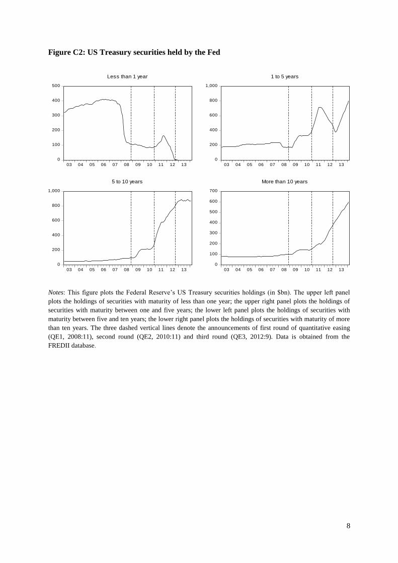
8

Figure C2: US Treasury securities held by the Fed

Notes: This figure plots the Federal Reserve’s US Treasury securities holdings (in $bn). The upper left panel

plots the holdings of securities with maturity of less than one year; the upper right panel plots the holdings of

securities with maturity between one and five years; the lower left panel plots the holdings of securities with

maturity between five and ten years; the lower right panel plots the holdings of securities with maturity of more

than ten years. The three dashed vertical lines denote the announcements of first round of quantitative easing

(QE1, 2008:11), second round (QE2, 2010:11) and third round (QE3, 2012:9). Data is obtained from the

FREDII database.

0

100

200

300

400

500

03 04 05 06 07 08 09 10 11 12 13

Less than 1 year

0

200

400

600

800

1,000

03 04 05 06 07 08 09 10 11 12 13

1 to 5 years

0

200

400

600

800

1,000

03 04 05 06 07 08 09 10 11 12 13

5 to 10 years

0

100

200

300

400

500

600

700

03 04 05 06 07 08 09 10 11 12 13

More than 10 years

9

Table C1: Descriptive statistics and unit root tests

Panel A

Variables 1985:1–2014:2 1985:1–2007:7

Mean St. dev. Min. Max. Mean St. dev. Min. Max.

1,ty -0.0219 0.5397 -2.9858 2.0324 -0.0106 0.5971 -2.9858 2.0324

120,ts 2.1306 1.3374 -1.0859 5.0091 1.9888 1.4003 -1.0859 5.0091

60,ts 1.4257 1.0714 -1.5288 4.4923 1.4530 1.1549 -1.5288 4.4923

24,ts 0.7751 0.8091 -1.7930 3.6581 0.8926 0.8636 -1.7930 3.6581

i

ir 0.9893 3.5285 -12.8149 22.3965 1.6556 2.9451 -12.8150 12.9246

trb -0.1760 0.8809 -2.7729 2.4335 -0.1089 0.9239 -2.4029 2.4335

tFFR -0.0237 0.2066 -0.9600 0.8700 -0.0115 0.2136 -0.6600 0.8700

U

tFFR -0.0313 0.0933 -0.6265 0.3300 -0.0414 0.1017 -0.6265 0.3125

tMB 0.8570 2.3134 -8.4381 25.9621 0.5484 0.5657 -2.6733 3.8956

U

tMB -0.0000 1.6363 -9.6332 12.7958 -0.1033 0.7291 -4.3168 2.5903

Panel B

Variables ADF constant ADF constant & trend PP constant PP constant & trend

1,ty -3.69 [11]*** -3.68 [11]** -27.39 [7]*** -27.36 [7]***

120,ts -4.08 [12]*** -4.08 [12]*** -4.28 [8]*** -4.27 [8] ***

60,ts -4.15 [12]*** -4.30 [12]*** -5.57 [7]*** -5.90 [8]***

24,ts -4.09 [12]*** -5.04 [12]*** -8.07 [9]*** -9.19 [9]***

i

ir -2.81 [14]* -3.64 [14]** -9.94 [4]*** -11.12 [4]***

trb -4.46 [15]*** -4.45 [15]*** -6.38 [9]*** -6.38 [9]***

tFFR -5.01 [4]*** -5.00 [4]*** -11.64 [10]*** -11.63 [10]***

U

tFFR -2.58 [11]* -4.68 [14]*** -14.65 [5]*** -15.62 [7]***

tMB -5.43 [8]*** -7.59 [6]*** -8.85 [5]*** -9.00 [6]***

U

tMB -18.59 [0]*** -18.70 [0]*** -18.59 [2]*** -18.70 [0]***

Notes: Panel A of this table reports the summary statistics for variables used for the benchmark VAR

estimations as well as our four monetary policy actions indicators over the full sample period (1985:1 –

2014:2) and pre-crisis period (1985:1 – 2007:7); the first difference in 1-month Treasury bill rate (∆y1), the

yield spread between 10-, 5- and 2-year Treasury bonds and the 1-month Treasury bill (s120, s60 and s24,

respectively), the real interest rate (ri) and the relative bill rate (rb); the change in the Federal funds rate

(∆FFR), the unexpected FFR change (∆FFRU), the change in log monetary base (∆MB) and the unexpected

change in log monetary base (∆MBU). Due to data availability on FFR futures, in the case of the unexpected

change in the FFR, the full sample commences on 1989:2. Panel B of this table reports the full sample test

statistics for the augmented Dickey-Fuller (ADF) and Phillips Perron (PP) unit root tests with (a) constant

and (b) constant and trend. In brackets we report the lag-length of the ADF test, based on Akaike

information criterion, and the Newey-West bandwidth for the PP test. ***, **, * denote 1%, 5% and 10%

level of significance, respectively.

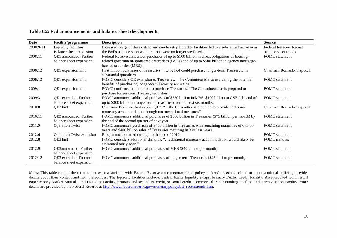
10

Table C2: Fed announcements and balance sheet developments Date Facility/programme Description Source

2008:9-11 Liquidity facilities:

Balance sheet expansion

Increased usage of the existing and newly setup liquidity facilities led to a substantial increase in

the Fed’s balance sheet as operations were no longer sterilised.

Federal Reserve: Recent

balance sheet trends

2008:11 QE1 announced: Further

balance sheet expansion

Federal Reserve announces purchases of up to $100 billion in direct obligations of housing-

related government-sponsored enterprises (GSEs) and of up to $500 billion in agency mortgage-

backed securities (MBS).

FOMC statement

2008:12 QE1 expansion hint First hint on purchases of Treasuries: “…the Fed could purchase longer-term Treasury…in

substantial quantities”.

Chairman Bernanke’s speech

2008:12 QE1 expansion hint FOMC considers QE extension to Treasuries: “The Committee is also evaluating the potential

benefits of purchasing longer-term Treasury securities”.

FOMC statement

2009:1 QE1 expansion hint FOMC confirms the intention to purchase Treasuries: “The Committee also is prepared to

purchase longer-term Treasury securities”.

FOMC statement

2009:3 QE1 extended: Further

balance sheet expansion

FOMC announces additional purchases of $750 billion in MBS, $100 billion in GSE debt and of

up to $300 billion in longer-term Treasuries over the next six months.

FOMC statement

2010:8 QE2 hint Chairman Bernanke hints about QE2: “…the Committee is prepared to provide additional

monetary accommodation through unconventional measures”.

Chairman Bernanke’s speech

2010:11 QE2 announced: Further

balance sheet expansion

FOMC announces additional purchases of $600 billion in Treasuries ($75 billion per month) by

the end of the second quarter of next year.

FOMC statement

2011:9 Operation Twist FOMC announces purchases of $400 billion in Treasuries with remaining maturities of 6 to 30

years and $400 billion sales of Treasuries maturing in 3 or less years.

FOMC statement

2012:6 Operation Twist extension Programme extended through to the end of 2012. FOMC statement

2012:8 QE3 hint FOMC considers additional stimulus: “…additional monetary accommodation would likely be

warranted fairly soon.”

FOMC minutes

2012:9 QE3announced: Further

balance sheet expansion

FOMC announces additional purchases of MBS ($40 billion per month). FOMC statement

2012:12 QE3 extended: Further

balance sheet expansion

FOMC announces additional purchases of longer-term Treasuries ($45 billion per month). FOMC statement

Notes: This table reports the months that were associated with Federal Reserve announcements and policy makers’ speeches related to unconventional policies, provides

details about their content and lists the sources. The liquidity facilities include: central banks liquidity swaps, Primary Dealer Credit Facility, Asset-Backed Commercial

Paper Money Market Mutual Fund Liquidity Facility, primary and secondary credit, seasonal credit, Commercial Paper Funding Facility, and Term Auction Facility. More

details are provided by the Federal Reserve at http://www.federalreserve.gov/monetarypolicy/bst_recenttrends.htm.

11

Table C3: Impact of macroeconomic news on monetary policy indicators

Macroeconomic surprise 1991:10 – 2014:2

FFR UFFR MB UMB

CPI inflation 0.064

(0.087)

-0.050

(0.041)

-2.883

(2.448)

-2.160

(1.761)

Core CPI inflation 0.002

(0.148)

0.038

(0.046)

-0.030

(2.092)

1.190

(1.581)

Nonfarm payrolls 0.007

(0.012)

-0.005

(0.005)

-0.083

(0.161)

-0.050

(0.095)

Industrial production 0.020

(0.031)

-0.020*

(0.011)

-0.286

(0.448)

-0.076

(0.419)

Retail sales excl. autos 0.002

(0.018)

0.009

(0.009)

0.286

(0.494)

0.437

(0.511)

R2

0.006 0.020 0.026 0.032

1991:10 – 2007:7

CPI inflation -0.002

(0.091)

-0.064

(0.044)

0.337

(0.452)

0.991*

(0.599)

Core CPI inflation -0.156

(0.169)

0.090

(0.057)

-0.218

(0.527)

-0.344

(0.741)

Nonfarm payrolls 0.002

(0.014)

-0.005

(0.006)

0.019

(0.038)

0.009

(0.048)

Industrial production 0.037

(0.045)

-0.010

(0.018)

-0.158

(0.106)

-0.220

(0.180)

Retail sales excl. autos -0.015

(0.029)

0.022

(0.016)

-0.112

(0.200)

-0.014

(0.321)

R2

0.012 0.024 0.014 0.035

Notes: This table reports the estimated parameters from regressions of our monetary policy actions

indicators on macroeconomic surprises. The monetary indicators are the change in the Federal funds rate

(∆FFR), the unexpected FFR change (∆FFRU), the change in log monetary base (∆MB) and the unexpected

change in log monetary base (∆MBU). The macroeconomic surprises relate to Reuters Economic Polls and

are calculated based on 'Actual' (the actual value that was reported by the primary source) minus 'Median

Forecast' (the forecast figure from the polls prior to the announcement) after the actual value is released.

The following macroeconomic variables are considered: CPI inflation, core CPI inflation, change in

nonfarm payrolls, growth rate of industrial production and growth rate of retail sales (excluding autos). The

upper panel of the table provides the full sample (1991:10 – 2014:2) estimates while the pre-crisis period

(1991:10 – 2007:7) estimates are shown in the lower panel. Due to data availability on macroeconomic

surprises, the full sample commences in 1991:10. Data is obtained from the Datastream. ***, **, * denote

1%, 5% and 10% level of significance, respectively.

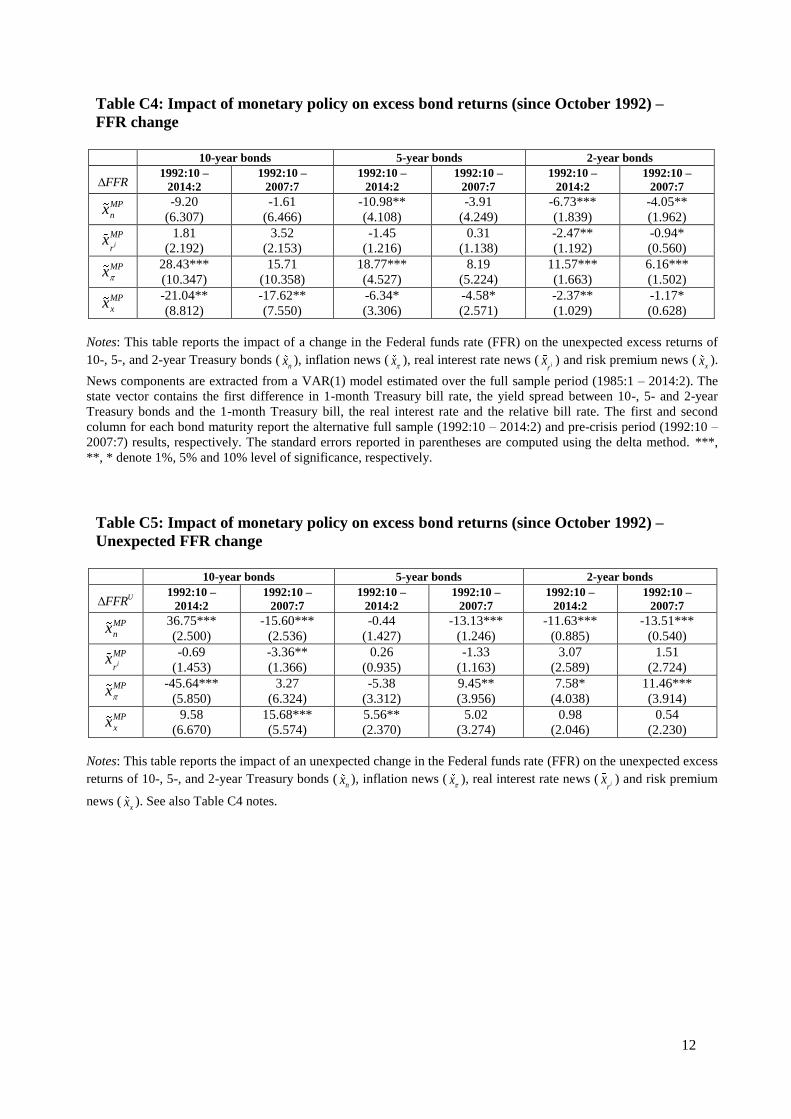
12

Table C4: Impact of monetary policy on excess bond returns (since October 1992) –

FFR change

10-year bonds 5-year bonds 2-year bonds

FFR 1992:10 –

2014:2

1992:10 –

2007:7

1992:10 –

2014:2

1992:10 –

2007:7

1992:10 –

2014:2

1992:10 –

2007:7

MP

nx -9.20

(6.307)

-1.61

(6.466)

-10.98**

(4.108)

-3.91

(4.249)

-6.73***

(1.839)

-4.05**

(1.962)

i

MP

rx

1.81

(2.192)

3.52

(2.153)

-1.45

(1.216)

0.31

(1.138)

-2.47**

(1.192)

-0.94*

(0.560)

MPx 28.43***

(10.347)

15.71

(10.358)

18.77***

(4.527)

8.19

(5.224)

11.57***

(1.663)

6.16***

(1.502)

MP

xx -21.04**

(8.812)

-17.62**

(7.550)

-6.34*

(3.306)

-4.58*

(2.571)

-2.37**

(1.029)

-1.17*

(0.628)

Notes: This table reports the impact of a change in the Federal funds rate (FFR) on the unexpected excess returns of

10-, 5-, and 2-year Treasury bonds (nx ), inflation news ( x ), real interest rate news ( ir

x ) and risk premium news (xx ).

News components are extracted from a VAR(1) model estimated over the full sample period (1985:1 – 2014:2). The

state vector contains the first difference in 1-month Treasury bill rate, the yield spread between 10-, 5- and 2-year

Treasury bonds and the 1-month Treasury bill, the real interest rate and the relative bill rate. The first and second

column for each bond maturity report the alternative full sample (1992:10 – 2014:2) and pre-crisis period (1992:10 –

2007:7) results, respectively. The standard errors reported in parentheses are computed using the delta method. ***,

**, * denote 1%, 5% and 10% level of significance, respectively.

Table C5: Impact of monetary policy on excess bond returns (since October 1992) –

Unexpected FFR change

10-year bonds 5-year bonds 2-year bonds

UFFR 1992:10 –

2014:2

1992:10 –

2007:7

1992:10 –

2014:2

1992:10 –

2007:7

1992:10 –

2014:2

1992:10 –

2007:7

MP

nx 36.75***

(2.500)

-15.60***

(2.536)

-0.44

(1.427)

-13.13***

(1.246)

-11.63***

(0.885)

-13.51***

(0.540)

i

MP

rx

-0.69

(1.453)

-3.36**

(1.366)

0.26

(0.935)

-1.33

(1.163)

3.07

(2.589)

1.51

(2.724)

MPx -45.64***

(5.850)

3.27

(6.324)

-5.38

(3.312)

9.45**

(3.956)

7.58*

(4.038)

11.46***

(3.914)

MP

xx 9.58

(6.670)

15.68***

(5.574)

5.56**

(2.370)

5.02

(3.274)

0.98

(2.046)

0.54

(2.230)

Notes: This table reports the impact of an unexpected change in the Federal funds rate (FFR) on the unexpected excess

returns of 10-, 5-, and 2-year Treasury bonds (nx ), inflation news ( x ), real interest rate news ( ir

x ) and risk premium

news (xx ). See also Table C4 notes.

13

Table C6: Variance decomposition for excess bond returns – alternative VAR specification [1] – adding industrial production growth

10-year bonds 5-year bonds 2-year bonds

1985:1–2014:2 1985:1–2007:7 1985:1–2014:2 1985:1–2007:7 1985:1–2014:2 1985:1–2007:7

Var x 0.832***

(0.264)

0.814***

(0.246)

1.111**

(0.433)

1.128**

(0.444)

1.636**

(0.787)

1.708**

(0.697)

2 , irCov x x

-0.086

(0.083)

-0.085

(0.086)

-0.190

(0.192)

-0.226

(0.186)

-0.698

(0.717)

-0.685

(0.582)

2 , xCov x x 0.048

(0.284)

0.113

(0.216)

-0.102

(0.356)

-0.017

(0.338)

-0.592

(0.472)

-0.377

(0.436)

irVar x 0.018*

(0.010)

0.017

(0.012)

0.039*

(0.023)

0.035

(0.024)

0.272*

(0.148)

0.145

(0.107)

2 ,i xrCov x x -0.068

(0.056)

-0.103*

(0.060)

0.026

(0.068)

-0.050

(0.069)

0.269

(0.180)

0.102

(0.129)

xVar x 0.256

(0.167)

0.244

(0.184)

0.117

(0.101)

0.131

(0.115)

0.113

(0.079)

0.107

(0.074)

2R x 0.795***

(0.153)

0.842***

(0.147)

0.837***

(0.114)

0.897***

(0.089)

0.600**

(0.157)

0.811***

(0.102)

2ir

R x 0.197

(0.145)

0.338**

(0.151)

0.049

(0.132)

0.310

(0.197)

0.012

(0.089)

0.147

(0.239)

2

xR x 0.236

(0.203)

0.254

(0.197)

0.054

(0.219)

0.073

(0.243)

0.021

(0.134)

0.009

(0.091)

Notes: This table reports the variance decomposition of unexpected excess returns of 10-, 5-, and 2-year Treasury bonds into the variances of inflation news ( x ), real

interest rate news ( irx ), risk premium news (

xx ) and the covariances between these three components. News components are extracted from a VAR(1) model where

the state vector contains the first difference in 1-month Treasury bill rate, the yield spread between 10-, 5- and 2-year Treasury bonds and the 1-month Treasury bill,

the real interest rate, the first difference in log industrial production index and the relative bill rate. The first and second column for each bond maturity report the full

sample (1985:1 – 2014:2) and pre-crisis period (1985:1 – 2007:7) results, respectively. R2 values are obtained from regressions of unexpected excess returns on each

news component. The standard errors reported in parentheses are computed using the delta method. ***, **, * denote 1%, 5% and 10% level of significance,

respectively.

14

Table C7: Variance decomposition for excess bond returns – alternative VAR specification [2] – adding unemployment rate

10-year bonds 5-year bonds 2-year bonds

1985:1–2014:2 1985:1–2007:7 1985:1–2014:2 1985:1–2007:7 1985:1–2014:2 1985:1–2007:7

Var x 0.838**

(0.397)

1.578

(0.978)

0.833**

(0.361)

1.703*

(0.894)

1.269**

(0.610)

1.797**

(0.761)

2 , irCov x x

0.227

(0.183)

-0.093

(0.180)

0.199

(0.174)

-0.186

(0.302)

-0.357

(0.472)

-0.632

(0.625)

2 , xCov x x -0.264

(0.510)

-0.688

(1.206)

-0.280

(0.385)

-0.709

(0.963)

-0.509

(0.386)

-0.495

(0.503)

irVar x 0.063

(0.051)

0.012

(0.008)

0.133*

(0.080)

0.026

(0.019)

0.303**

(0.122)

0.134

(0.105)

2 ,i xrCov x x -0.061

(0.148)

-0.026

(0.076)

0.004

(0.129)

0.006

(0.104)

0.193

(0.151)

0.106

(0.140)

xVar x 0.197

(0.159)

0.217

(0.303)

0.110

(0.096)

0.160

(0.196)

0.102

(0.075)

0.090

(0.062)

2R x 0.801***

(0.152)

0.894***

(0.107)

0.755***

(0.152)

0.926***

(0.067)

0.550***

(0.175)

0.846***

(0.088)

2ir

R x 0.339**

(0.150)

0.193

(0.327)

0.415**

(0.188)

0.162

(0.362)

0.161

(0.271)

0.124

(0.249)

2

xR x 0.006

(0.084)

0.090

(0.304)

0.007

(0.103)

0.229

(0.449)

0.031

(0.170)

0.121

(0.349)

Notes: This table reports the variance decomposition of unexpected excess returns of 10-, 5-, and 2-year Treasury bonds into the variances of inflation news ( x ), real

interest rate news ( irx ), risk premium news (

xx ) and the covariances between these three components. News components are extracted from a VAR(1) model where

the state vector contains the first difference in 1-month Treasury bill rate, the yield spread between 10-, 5- and 2-year Treasury bonds and the 1-month Treasury bill,

the real interest rate, the civilian unemployment rate and the relative bill rate. See also Table C6 notes.

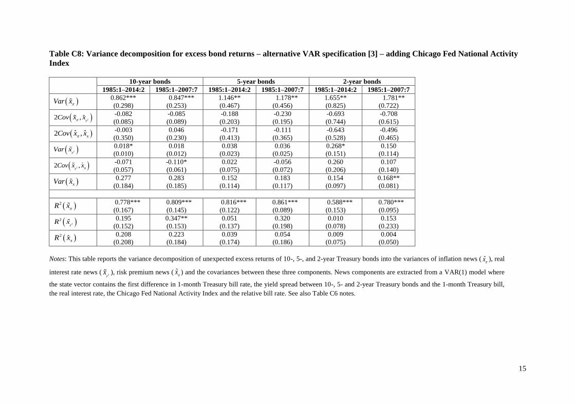
15

Table C8: Variance decomposition for excess bond returns – alternative VAR specification [3] – adding Chicago Fed National Activity

Index

10-year bonds 5-year bonds 2-year bonds

1985:1–2014:2 1985:1–2007:7 1985:1–2014:2 1985:1–2007:7 1985:1–2014:2 1985:1–2007:7

Var x 0.862***

(0.298)

0.847***

(0.253)

1.146**

(0.467)

1.178**

(0.456)

1.655**

(0.825)

1.781**

(0.722)

2 , irCov x x

-0.082

(0.085)

-0.085

(0.089)

-0.188

(0.203)

-0.230

(0.195)

-0.693

(0.744)

-0.708

(0.615)

2 , xCov x x -0.003

(0.350)

0.046

(0.230)

-0.171

(0.413)

-0.111

(0.365)

-0.643

(0.528)

-0.496

(0.465)

irVar x 0.018*

(0.010)

0.018

(0.012)

0.038

(0.023)

0.036

(0.025)

0.268*

(0.151)

0.150

(0.114)

2 ,i xrCov x x -0.071

(0.057)

-0.110*

(0.061)

0.022

(0.075)

-0.056

(0.072)

0.260

(0.206)

0.107

(0.140)

xVar x 0.277

(0.184)

0.283

(0.185)

0.152

(0.114)

0.183

(0.117)

0.154

(0.097)

0.168**

(0.081)

2R x 0.778***

(0.167)

0.809***

(0.145)

0.816***

(0.122)

0.861***

(0.089)

0.588***

(0.153)

0.780***

(0.095)

2ir

R x 0.195

(0.152)

0.347**

(0.153)

0.051

(0.137)

0.320

(0.198)

0.010

(0.078)

0.153

(0.233)

2

xR x 0.208

(0.208)

0.223

(0.184)

0.039

(0.174)

0.054

(0.186)

0.009

(0.075)

0.004

(0.050)

Notes: This table reports the variance decomposition of unexpected excess returns of 10-, 5-, and 2-year Treasury bonds into the variances of inflation news ( x ), real

interest rate news ( irx ), risk premium news (

xx ) and the covariances between these three components. News components are extracted from a VAR(1) model where

the state vector contains the first difference in 1-month Treasury bill rate, the yield spread between 10-, 5- and 2-year Treasury bonds and the 1-month Treasury bill,

the real interest rate, the Chicago Fed National Activity Index and the relative bill rate. See also Table C6 notes.

16

Table C9: Variance decomposition for excess bond returns – alternative VAR specification [4] – adding Chicago Fed Adjusted National

Financial Conditions Index

10-year bonds 5-year bonds 2-year bonds

1985:1–2014:2 1985:1–2007:7 1985:1–2014:2 1985:1–2007:7 1985:1–2014:2 1985:1–2007:7

Var x 0.847**

(0.341)

0.757***

(0.218)

1.181**

(0.568)

1.059**

(0.414)

1.911*

(1.118)

1.860**

(0.814)

2 , irCov x x

-0.124

(0.136)

-0.085

(0.092)

-0.283

(0.323)

-0.241

(0.212)

-1.106

(1.201)

-0.990

(0.782)

2 , xCov x x -0.079

(0.470)

0.064

(0.270)

-0.280

(0.559)

-0.082

(0.359)

-0.876

(0.717)

-0.538

(0.502)

irVar x 0.025

(0.017)

0.023

(0.015)

0.062

(0.052)

0.054

(0.038)

0.419

(0.320)

0.278

(0.198)

2 ,i xrCov x x -0.019

(0.099)

-0.052

(0.079)

0.115

(0.158)

0.031

(0.116)

0.471

(0.366)

0.254

(0.220)

xVar x 0.351

(0.241)

0.293

(0.218)

0.206

(0.174)

0.178

(0.166)

0.182

(0.134)

0.135

(0.104)

2R x 0.656***

(0.248)

0.737***

(0.218)

0.685**

(0.207)

0.761***

(0.198)

0.443**

(0.185)

0.646***

(0.180)

2ir

R x 0.090

(0.118)

0.092

(0.145)

0.008

(0.049)

0.047

(0.129)

0.025

(0.109)

0.029

(0.112)

2

xR x 0.260

(0.197)

0.305*

(0.171)

0.074

(0.204)

0.131

(0.251)

0.002

(0.035)

0.000

(0.016)

Notes: This table reports the variance decomposition of unexpected excess returns of 10-, 5-, and 2-year Treasury bonds into the variances of inflation news ( x ), real

interest rate news ( irx ), risk premium news ( xx ) and the covariances between these three components. News components are extracted from a VAR(1) model where

the state vector contains the first difference in 1-month Treasury bill rate, the yield spread between 10-, 5- and 2-year Treasury bonds and the 1-month Treasury bill,

the real interest rate, the Chicago Fed Adjusted National Financial Conditions Index and the relative bill rate. See also Table C6 notes.

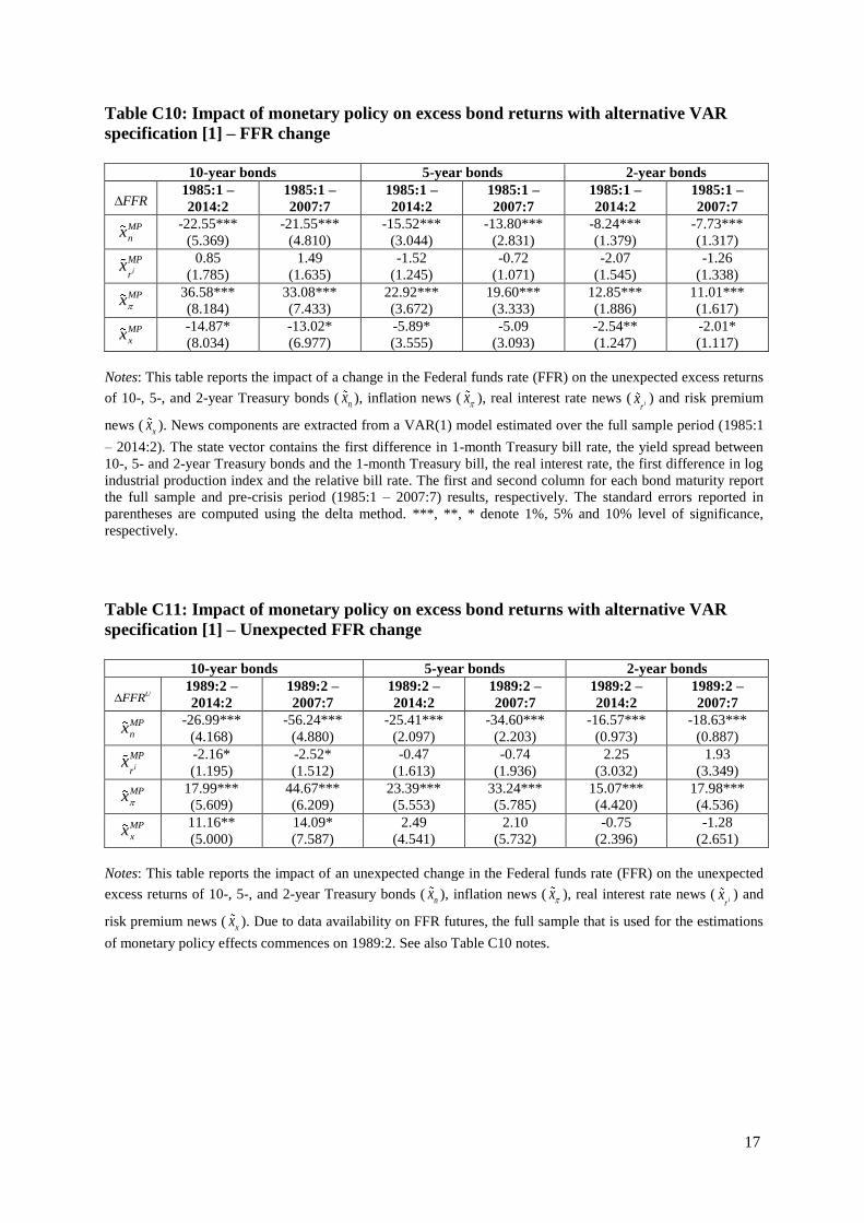
17

Table C10: Impact of monetary policy on excess bond returns with alternative VAR

specification [1] – FFR change

10-year bonds 5-year bonds 2-year bonds

FFR 1985:1 –

2014:2

1985:1 –

2007:7 1985:1 –

2014:2

1985:1 –

2007:7

1985:1 –

2014:2

1985:1 –

2007:7

MP

nx -22.55***

(5.369)

-21.55***

(4.810)

-15.52***

(3.044)

-13.80***

(2.831)

-8.24***

(1.379)

-7.73***

(1.317)

i

MP

rx

0.85

(1.785)

1.49

(1.635)

-1.52

(1.245)

-0.72

(1.071)

-2.07

(1.545)

-1.26

(1.338)

MPx 36.58***

(8.184)

33.08***

(7.433)

22.92***

(3.672)

19.60***

(3.333)

12.85***

(1.886)

11.01***

(1.617)

MP

xx -14.87*

(8.034)

-13.02*

(6.977)

-5.89*

(3.555)

-5.09

(3.093)

-2.54**

(1.247)

-2.01*

(1.117)

Notes: This table reports the impact of a change in the Federal funds rate (FFR) on the unexpected excess returns

of 10-, 5-, and 2-year Treasury bonds (nx ), inflation news ( x ), real interest rate news ( ir

x ) and risk premium

news (xx ). News components are extracted from a VAR(1) model estimated over the full sample period (1985:1

– 2014:2). The state vector contains the first difference in 1-month Treasury bill rate, the yield spread between

10-, 5- and 2-year Treasury bonds and the 1-month Treasury bill, the real interest rate, the first difference in log

industrial production index and the relative bill rate. The first and second column for each bond maturity report

the full sample and pre-crisis period (1985:1 – 2007:7) results, respectively. The standard errors reported in

parentheses are computed using the delta method. ***, **, * denote 1%, 5% and 10% level of significance,

respectively.

Table C11: Impact of monetary policy on excess bond returns with alternative VAR

specification [1] – Unexpected FFR change

10-year bonds 5-year bonds 2-year bonds

UFFR 1989:2 –

2014:2

1989:2 –

2007:7 1989:2 –

2014:2

1989:2 –

2007:7

1989:2 –

2014:2

1989:2 –

2007:7

MP

nx -26.99***

(4.168)

-56.24***

(4.880)

-25.41***

(2.097)

-34.60***

(2.203)

-16.57***

(0.973)

-18.63***

(0.887)

i

MP

rx

-2.16*

(1.195)

-2.52*

(1.512)

-0.47

(1.613)

-0.74

(1.936)

2.25

(3.032)

1.93

(3.349)

MPx 17.99***

(5.609)

44.67***

(6.209)

23.39***

(5.553)

33.24***

(5.785)

15.07***

(4.420)

17.98***

(4.536)

MP

xx 11.16**

(5.000)

14.09*

(7.587)

2.49

(4.541)

2.10

(5.732)

-0.75

(2.396)

-1.28

(2.651)

Notes: This table reports the impact of an unexpected change in the Federal funds rate (FFR) on the unexpected

excess returns of 10-, 5-, and 2-year Treasury bonds (nx ), inflation news ( x ), real interest rate news ( ir

x ) and

risk premium news ( xx ). Due to data availability on FFR futures, the full sample that is used for the estimations

of monetary policy effects commences on 1989:2. See also Table C10 notes.

18

Table C12: Impact of monetary policy on excess bond returns with alternative VAR

specification [1] – MB change

10-year bonds 5-year bonds 2-year bonds

MB 1985:1 –

2014:2

1985:1 –

2007:7 1985:1 –

2014:2

1985:1 –

2007:7

1985:1 –

2014:2

1985:1 –

2007:7

MP

nx 0.92***

(0.337)

-1.08

(1.055)

0.79***

(0.114)

0.76

(0.538)

0.31***

(0.041)

0.53**

(0.212)

i

MP

rx

0.17*

(0.100)

-0.54**

(0.267)

0.26**

(0.090)

-0.48**

(0.211)

0.28***

(0.095)

-0.48**

(0.205)

MPx -2.13***

(0.360)

0.67

(1.530)

-1.49***

(0.205)

-0.21

(0.783)

-0.80***

(0.122)

0.13

(0.396)

MP

xx 1.05*

(0.598)

0.95

(0.858)

0.45*

(0.239)

-0.07

(0.383)

0.21***

(0.073)

-0.17

(0.151)

Notes: This table reports the impact of a change in log monetary base (MB) on the unexpected excess returns of 10-,

5-, and 2-year Treasury bonds (nx ), inflation news ( x ), real interest rate news ( ir

x ) and risk premium news (xx ).

See also Table C10 notes.

Table C13: Impact of monetary policy on excess bond returns with alternative VAR

specification [1] – Unexpected MB change

10-year bonds 5-year bonds 2-year bonds

UMB 1985:1 –

2014:2

1985:1 –

2007:7 1985:1 –

2014:2

1985:1 –

2007:7

1985:1 –

2014:2

1985:1 –

2007:7

MP

nx 1.20***

(0.198)

1.16**

(0.557)

1.18***

(0.087)

1.07***

(0.329)

0.48***

(0.034)

0.34**

(0.146)

i

MP

rx

0.31**

(0.123)

0.02

(0.253)

0.34**

(0.138)

-0.30

(0.205)

0.31*

(0.157)

-0.53***

(0.177)

MPx -2.17**

(0.588)

1.62

(1.235)

-1.86***

(0.406)

0.40

(1.716)

-1.00***

(0.229)

0.56*

(0.314)

MP

xx 0.67

(0.571)

-2.81**

(1.125)

0.34

(0.300)

-1.17**

(0.518)

0.21**

(0.104)

-0.37**

(0.153)

Notes: This table reports the impact of an unexpected change in log monetary base (MB) on the unexpected

excess returns of 10-, 5-, and 2-year Treasury bonds (nx ), inflation news ( x ), real interest rate news ( ir

x ) and

risk premium news (xx ). See also Table C10 notes.

19

Table C14: Impact of monetary policy on excess bond returns with alternative VAR

specification [2] – FFR change

10-year bonds 5-year bonds 2-year bonds

FFR 1985:1 –

2014:2

1985:1 –

2007:7 1985:1 –

2014:2

1985:1 –

2007:7

1985:1 –

2014:2

1985:1 –

2007:7

MP

nx -21.10***

(5.042)

-20.79***

(5.145)

-15.45***

(3.014)

-13.60***

(2.919)

-8.51***

(1.351)

-7.83***

(1.293)

i

MP

rx

5.37*

(3.156)

5.39*

(2.794)

2.76

(2.076)

2.75

(1.782)

-0.08

(1.682)

0.29

(1.473)

MPx 35.62***

(9.892)

31.95***

(8.634)

20.30***

(4.258)

17.35***

(3.626)

11.17***

(2.053)

9.71***

(1.744)

MP

xx -19.89*

(10.627)

-16.55*

(9.327)

-7.61*

(4.250)

-6.50*

(3.682)

-2.58**

(1.243)

-2.16*

(1.121)

Notes: This table reports the impact of a change in the Federal funds rate (FFR) on the unexpected excess returns

of 10-, 5-, and 2-year Treasury bonds (nx ), inflation news ( x ), real interest rate news ( ir

x ) and risk premium

news (xx ). News components are extracted from a VAR(1) model estimated over the full sample period (1985:1

– 2014:2). The state vector contains the first difference in 1-month Treasury bill rate, the yield spread between

10-, 5- and 2-year Treasury bonds and the 1-month Treasury bill, the real interest rate, the civilian

unemployment rate and the relative bill rate. The first and second column for each bond maturity report the full

sample and pre-crisis period (1985:1 – 2007:7) results, respectively. The standard errors reported in parentheses

are computed using the delta method. ***, **, * denote 1%, 5% and 10% level of significance, respectively.

Table C15: Impact of monetary policy on excess bond returns with alternative VAR

specification [2] – Unexpected FFR change

10-year bonds 5-year bonds 2-year bonds

UFFR 1989:2 –

2014:2

1989:2 –

2007:7 1989:2 –

2014:2

1989:2 –

2007:7

1989:2 –

2014:2

1989:2 –

2007:7

MP

nx -24.22***

(1.999)

-54.28***

(4.049)

-25.73***

(1.427)

-34.50***

(1.960)

-17.38***

(0.709)

-19.11***

(0.789)

i

MP

rx

10.55**

(4.625)

17.92**

(7.532)

11.23**

(3.915)

14.76***

(4.968)

6.61*

(3.386)

7.18*

(3.660)

MPx 17.37

(11.754)

44.26**

(18.447)

16.94**

(7.015)

23.77***

(8.448)

11.91**

(4.563)

13.46***

(4.722)

MP

xx -3.70

(12.333)

-7.90

(21.634)

-2.44

(6.189)

-4.03

(8.376)

-1.14

(2.461)

-1.53

(2.665)

Notes: This table reports the impact of an unexpected change in the Federal funds rate (FFR) on the unexpected

excess returns of 10-, 5-, and 2-year Treasury bonds (nx ), inflation news ( x ), real interest rate news ( ir

x ) and

risk premium news (xx ). Due to data availability on FFR futures, the full sample that is used for the estimations

of monetary policy effects commences on 1989:2. See also Table C14 notes.

20

Table C16: Impact of monetary policy on excess bond returns with alternative VAR

specification [2] – MB change

10-year bonds 5-year bonds 2-year bonds

MB 1985:1 –

2014:2

1985:1 –

2007:7 1985:1 –

2014:2

1985:1 –

2007:7

1985:1 –

2014:2

1985:1 –

2007:7

MP

nx 0.79***

(0.290)

-0.88

(1.113)

0.78***

(0.120)

0.71

(0.549)

0.33***

(0.041)

0.47**

(0.210)

i

MP

rx

-0.33

(0.228)

1.11

(0.744)

-0.16

(0.152)

0.42

(0.363)

0.11

(0.103)

-0.02

(0.203)

MPx -2.12***

(0.614)

0.87

(2.292)

-1.22***

(0.278)

-0.76

(0.862)

-0.64***

(0.130)

-0.39

(0.367)

MP

xx 1.66*

(0.850)

-1.09

(1.755)

0.60*

(0.318)

-0.37

(0.485)

0.19**

(0.074)

-0.07

(0.128)

Notes: This table reports the impact of a change in log monetary base (MB) on the unexpected excess returns of

10-, 5-, and 2-year Treasury bonds (nx ), inflation news ( x ), real interest rate news ( ir

x ) and risk premium news

(xx ). See also Table C14 notes.

Table C17: Impact of monetary policy on excess bond returns with alternative VAR

specification [2] – Unexpected MB change

10-year bonds 5-year bonds 2-year bonds

UMB 1985:1 –

2014:2

1985:1 –

2007:7 1985:1 –

2014:2

1985:1 –

2007:7

1985:1 –

2014:2

1985:1 –

2007:7

MP

nx 1.05***

(0.104)

1.20**

(0.573)

1.19***

(0.049)

1.09***

(0.331)

0.51***

(0.019)

0.34**

(0.144)

i

MP

rx

0.06

(0.179)

0.09

(0.340)

0.01

(0.177)

-0.36

(0.277)

0.19

(0.154)

-0.42**

(0.183)

MPx -2.17***

(0.651)

1.56

(1.217)

-1.66***

(0.403)

0.41

(0.628)

-0.90***

(0.227)

0.44

(0.300)

MP

xx 1.06

(0.698)

-2.86**

(1.287)

0.46

(0.344)

-1.14**

(0.551)

0.20*

(0.102)

-0.36**

(0.160)

Notes: This table reports the impact of an unexpected change in log monetary base (MB) on the unexpected

excess returns of 10-, 5-, and 2-year Treasury bonds (nx ), inflation news ( x ), real interest rate news ( ir

x ) and

risk premium news (xx ). See also Table C14 notes.

21

Table C18: Impact of monetary policy on excess bond returns with alternative VAR

specification [3] – FFR change

10-year bonds 5-year bonds 2-year bonds

FFR 1985:1 –

2014:2

1985:1 –

2007:7 1985:1 –

2014:2

1985:1 –

2007:7

1985:1 –

2014:2

1985:1 –

2007:7

MP

nx -18.96***

(5.835)

-18.97***

(5.237)

-14.38***

(3.133)

-13.01***

(2.901)

-8.13***

(1.367)

-7.71***

(1.312)

i

MP

rx

0.86

(1.781)

1.31

(1.555)

-1.53

(1.246)

-0.81

(1.031)

-2.15

(1.507)

-1.39

(1.210)

MPx 35.29***

(8.262)

31.22***

(7.311)

22.44***

(3.694)

18.68***

(3.415)

12.77***

(1.815)

10.71***

(1.508)

MP

xx -17.18**

(8.642)

-13.56*

(7.047)

-6.53*

(3.623)

-4.86

(3.078)

-2.49**

(1.238)

-1.62**

(1.109)

Notes: This table reports the impact of a change in the Federal funds rate (FFR) on the unexpected excess returns

of 10-, 5-, and 2-year Treasury bonds (nx ), inflation news ( x ), real interest rate news ( ir

x ) and risk premium

news (xx ). News components are extracted from a VAR(1) model estimated over the full sample period (1985:1

– 2014:2). The state vector contains the first difference in 1-month Treasury bill rate, the yield spread between

10-, 5- and 2-year Treasury bonds and the 1-month Treasury bill, the real interest rate, the Chicago Fed National

Activity Index and the relative bill rate. The first and second column for each bond maturity report the full

sample and pre-crisis period (1985:1 – 2007:7) results, respectively. The standard errors reported in parentheses

are computed using the delta method. ***, **, * denote 1%, 5% and 10% level of significance, respectively.

Table C19: Impact of monetary policy on excess bond returns with alternative VAR

specification [3] – Unexpected FFR change

10-year bonds 5-year bonds 2-year bonds

UFFR 1989:2 –

2014:2

1989:2 –

2007:7 1989:2 –

2014:2

1989:2 –

2007:7

1989:2 –

2014:2

1989:2 –

2007:7

MP

nx -23.30***

(2.747)

-51.65***

(5.510)

-24.10***

(1.657)

-32.27***

(2.459)

-16.35***

(0.833)

-17.85***

(0.956)

i

MP

rx

-2.18**

(0.972)

-2.23

(1.534)

-0.76

(1.447)

-0.65

(2.052)

1.81

(2.796)

1.81

(3.323)

MPx 14.39***

(4.890)

44.13***

(6.105)

22.13***

(4.866)

32.95***

(5.810)

15.09***

(4.008)

17.80***

(4.437)

MP

xx 11.09**

(4.257)

9.75

(8.290)

2.73

(4.265)

-0.04

(5.957)

-0.55

(2.311)

-1.76

(2.604)

Notes: This table reports the impact of an unexpected change in the Federal funds rate (FFR) on the unexpected

excess returns of 10-, 5-, and 2-year Treasury bonds (nx ), inflation news ( x ), real interest rate news ( ir

x ) and

risk premium news (xx ). Due to data availability on FFR futures, the full sample that is used for the estimations

of monetary policy effects commences on 1989:2. See also Table C18 notes.

22

Table C20: Impact of monetary policy on excess bond returns with alternative VAR

specification [3] – MB change

10-year bonds 5-year bonds 2-year bonds

MB 1985:1 –

2014:2

1985:1 –

2007:7 1985:1 –

2014:2

1985:1 –

2007:7

1985:1 –

2014:2

1985:1 –

2007:7

MP

nx 0.57

(0.451)

-0.64

(1.009)

0.61***

(0.159)

0.97*

(0.538)

0.26***

(0.052)

0.61***

(0.216)

i

MP

rx

0.11

(0.139)

0.55**

(0.262)

0.23*

(0.130)

-0.46**

(0.199)

0.26*

(0.136)

-0.46**

(0.192)

MPx -2.33***

(0.546)

0.65

(1.487)

-1.60***

(0.299)

-0.30

(0.752)

-0.83***

(0.179)

0.03

(0.363)

MP

xx 1.65*

(0.869)

0.54

(0.910)

0.77**

(0.339)

-0.22

(0.382)

0.31***

(0.101)

-0.19

(0.130)

Notes: This table reports the impact of a change in log monetary base (MB) on the unexpected excess returns of

10-, 5-, and 2-year Treasury bonds (nx ), inflation news ( x ), real interest rate news ( ir

x ) and risk premium news

(xx ). See also Table C18 notes.

Table C21: Impact of monetary policy on excess bond returns with alternative VAR

specification [3] – Unexpected MB change

10-year bonds 5-year bonds 2-year bonds

UMB 1985:1 –

2014:2

1985:1 –

2007:7 1985:1 –

2014:2

1985:1 –

2007:7

1985:1 –

2014:2

1985:1 –

2007:7

MP

nx 0.98***

(0.143)

1.48**

(0.687)

1.12***

(0.063)

1.27***

(0.356)

0.48***

(0.023)

0.41***

(0.149)

i

MP

rx

0.22

(0.182)

-0.04

(0.237)

0.30

(0.200)

-0.31

(0.220)

0.29

(0.222)

-0.54**

(0.203)

MPx -2.54**

(0.940)

1.27

(1.211)

-2.09***

(0.573)

0.17

(0.776)

-1.09***

(0.332)

0.45

(0.358)

MP

xx 1.35

(0.897)

-2.71**

(1.108)

0.67

(0.428)

-1.13**

(0.545)

0.33**

(0.144)

-0.33*

(0.169)

Notes: This table reports the impact of an unexpected change in log monetary base (MB) on the unexpected

excess returns of 10-, 5-, and 2-year Treasury bonds (nx ), inflation news ( x ), real interest rate news ( ir

x ) and

risk premium news (xx ). See also Table C18 notes.

23

Table C22: Impact of monetary policy on excess bond returns with alternative VAR

specification [4] – FFR change

10-year bonds 5-year bonds 2-year bonds

FFR 1985:1 –

2014:2

1985:1 –

2007:7 1985:1 –

2014:2

1985:1 –

2007:7

1985:1 –

2014:2

1985:1 –

2007:7

MP

nx -21.10***

(4.647)

-22.97***

(4.684)

-15.62***

(2.962)

-14.93***

(2.832)

-8.36***

(1.356)

-8.11***

(1.291)

i

MP

rx

2.19

(1.931)

4.00*

(2.350)

-0.47

(1.282)

1.58

(1.829)

-1.27

(1.232)

0.73

(1.335)

MPx 29.89***

(7.858)

21.44**

(9.521)

19.77***

(3.788)

13.27***

(5.053)

11.46***

(1.524)

7.78***

(1.853)

MP

xx -10.98*

(6.620)

-2.47

(8.519)

-3.68

(3.204)

0.08

(4.018)

-1.83

(1.166)

-0.40

(1.233)

Notes: This table reports the impact of a change in the Federal funds rate (FFR) on the unexpected excess returns

of 10-, 5-, and 2-year Treasury bonds (nx ), inflation news ( x ), real interest rate news ( ir

x ) and risk premium

news (xx ). News components are extracted from a VAR(1) model estimated over the full sample period (1985:1

– 2014:2). The state vector contains the first difference in 1-month Treasury bill rate, the yield spread between

10-, 5- and 2-year Treasury bonds and the 1-month Treasury bill, the real interest rate, the Chicago Fed Adjusted

National Financial Conditions Index and the relative bill rate. The first and second column for each bond

maturity report the full sample and pre-crisis period (1985:1 – 2007:7) results, respectively. The standard errors

reported in parentheses are computed using the delta method. ***, **, * denote 1%, 5% and 10% level of

significance, respectively.

Table C23: Impact of monetary policy on excess bond returns with alternative VAR

specification [4] – Unexpected FFR change

10-year bonds 5-year bonds 2-year bonds

UFFR 1989:2 –

2014:2

1989:2 –

2007:7 1989:2 –

2014:2

1989:2 –

2007:7

1989:2 –

2014:2

1989:2 –

2007:7

MP

nx -27.84***

(3.035)

-54.34***

(3.379)

-27.17***

(1.769)

-34.90***

(1.776)

-18.02***

(0.889)

-19.34***

(0.735)

i

MP

rx

-2.08*

(1.149)

-0.89

(1.878)

-0.74

(2.154)

0.96

(2.066)

2.22

(3.735)

3.82

(3.288)

MPx 20.16***

(4.616)

36.53***

(8.092)

25.69***

(6.328)

28.27***

(6.107)

16.84***

(5.352)

15.26***

(4.436)

MP

xx 9.76**

(4.597)

18.69**

(7.541)

2.22

(5.006)

5.67

(5.649)

-1.04

(2.638)

0.26

(2.624)

Notes: This table reports the impact of an unexpected change in the Federal funds rate (FFR) on the unexpected

excess returns of 10-, 5-, and 2-year Treasury bonds (nx ), inflation news ( x ), real interest rate news ( ir

x ) and

risk premium news ( xx ). Due to data availability on FFR futures, the full sample that is used for the estimations

of monetary policy effects commences on 1989:2. See also Table C22 notes.

24

Table C24: Impact of monetary policy on excess bond returns with alternative VAR

specification [4] – MB change

10-year bonds 5-year bonds 2-year bonds

MB 1985:1 –

2014:2

1985:1 –

2007:7 1985:1 –

2014:2

1985:1 –

2007:7

1985:1 –

2014:2

1985:1 –

2007:7

MP

nx 0.48

(0.426)

-0.72

(1.008)

0.66***

(0.153)

0.85

(0.521)

0.29***

(0.053)

0.54**

(0.207)

i

MP

rx

0.23*

(0.121)

-0.18

(0.314)

0.32***

(0.114)

-0.08

(0.253)

0.34***

(0.118)

-0.10

(0.241)

MPx -2.30***

(0.390)

-1.37

(1.272)

-1.60***

(0.230)

-1.53**

(0.718)

-0.85***

(0.136)

-0.64*

(0.353)

MP

xx 1.60**

(0.703)

2.27*

(1.233)

0.62**

(0.280)

0.76

(0.533)

0.23***

(0.074)

-0.20

(0.158)

Notes: This table reports the impact of a change in log monetary base (MB) on the unexpected excess returns of

10-, 5-, and 2-year Treasury bonds (nx ), inflation news ( x ), real interest rate news ( ir

x ) and risk premium news

(xx ). See also Table C22 notes.

Table C25: Impact of monetary policy on excess bond returns with alternative VAR

specification [4] – Unexpected MB change

10-year bonds 5-year bonds 2-year bonds

UMB 1985:1 –

2014:2

1985:1 –

2007:7 1985:1 –

2014:2

1985:1 –

2007:7

1985:1 –

2014:2

1985:1 –

2007:7

MP

nx 0.72**

(0.304)

0.44

(0.814)

1.04***

(0.127)

0.72*

(0.427)

0.46***

(0.044)

0.21

(0.169)

i

MP

rx

0.61*

(0.339)

0.33

(0.327)

0.66*

(0.353)

-0.00

(0.347)

0.60*

(0.355)

-0.27

(0.296)

MPx -3.60**

(1.478)

0.47

(1.226)

-2.74***

(0.891)

-0.27

(0.921)

-1.49***

(0.477)

0.18

(0.437)

MP

xx 2.27

(1.458)

-1.23

(1.267)

1.05

(0.690)

-0.43

(0.723)

0.43**

(0.194)

-0.12

(0.209)

Notes: This table reports the impact of an unexpected change in log monetary base (MB) on the unexpected

excess returns of 10-, 5-, and 2-year Treasury bonds (nx ), inflation news ( x ), real interest rate news ( ir

x ) and

risk premium news (xx ). See also Table C22 notes.

25

Table C26: Impact of monetary policy on excess bond returns – Romer and Romer

policy shock

10-year bonds 5-year bonds 2-year bonds

RR 1985:1 – 2007:7 1985:1 – 2007:7 1985:1 – 2007:7

MP

nx -27.70***

(4.765)

-17.63***

(3.108)

-8.73***

(1.487)

i

MP

rx

2.21

(1.641)

-0.11

(1.006)

-0.78

(1.181)

MPx 39.12***

(7.343)

22.43***

(3.226)

11.24***

(1.421)

MP

xx -13.64**

(6.788)

-4.68

(3.036)

-1.73*

(1.027)

Notes: This table reports the impact of a monetary policy shock as measured by Romer and Romer (2004) on the

unexpected excess returns of 10-, 5-, and 2-year Treasury bonds (nx ), inflation news ( x ), real interest rate news

( irx ) and risk premium news (

xx ). News components are extracted from a VAR(1) model estimated over the full

sample period (1985:1 – 2014:2). The state vector contains the first difference in 1-month Treasury bill rate, the

yield spread between 10-, 5- and 2-year Treasury bonds and the 1-month Treasury bill, the real interest rate, and

the relative bill rate. The pre-crisis period (1985:1 – 2007:7) results are reported for each bond maturity. The

standard errors reported in parentheses are computed using the delta method. ***, **, * denote 1%, 5% and 10%

level of significance, respectively.

26

Table C27: Variance decomposition for excess bond returns – VAR(3)

10-year bonds 5-year bonds 2-year bonds

1985:1–2014:2 1985:1–2007:7 1985:1–2014:2 1985:1–2007:7 1985:1–2014:2 1985:1–2007:7

Var x 0.980***

(0.362)

1.042***

(0.370)

1.532**

(0.675)

1.386**

(0.576)

2.339*

(1.216)

1.847**

(0.892)

2 , irCov x x

-0.071

(0.094)

-0.049

(0.069)

-0.226

(0.272)

-0.120

(0.155)

-1.078

(1.120)

-0.429

(0.658)

2 , xCov x x -0.058

(0.387)

-0.122

(0.429)

-0.582

(0.684)

-0.493

(0.656)

-1.361

(0.838)

-0.997

(0.754)

irVar x 0.016*

(0.009)

0.008

(0.005)

0.041

(0.030)

0.015

(0.012)

0.371

(0.242)

0.101

(0.097)

2 ,i xrCov x x -0.020

(0.052)

-0.039

(0.040)

0.076

(0.107)

0.016

(0.073)

0.463

(0.360)

0.198

(0.239)

xVar x 0.153

(0.126)

0.161

(0.173)

0.159

(0.165)

0.195

(0.207)

0.266

(0.179)

0.279

(0.203)

2R x 0.856***

(0.114)

0.877***

(0.137)

0.831***

(0.131)

0.841***

(0.148)

0.536**

(0.194)

0.696***

(0.179)

2ir

R x 0.055

(0.096)

0.175

(0.184)

0.029

(0.113)

0.086

(0.171)

0.011

(0.091)

0.002

(0.088)

2

xR x 0.084

(0.222)

0.040

(0.160)

0.056

(0.244)

0.010

(0.096)

0.126

(0.252)

0.051

(0.159)

Notes: This table reports the variance decomposition of unexpected excess returns of 10-, 5-, and 2-year Treasury bonds into the variances of inflation news ( x ), real

interest rate news ( irx ), risk premium news ( xx ) and the covariances between these three components. News components are extracted from a VAR(3) model where

the state vector contains the first difference in 1-month Treasury bill rate, the yield spread between 10-, 5- and 2-year Treasury bonds and the 1-month Treasury bill,

the real interest rate and the relative bill rate. The first and second column for each bond maturity report the full sample (1985:1 – 2014:2) and pre-crisis period

(1985:1 – 2007:7) results, respectively. R2 values are obtained from regressions of unexpected excess returns on each news component. The standard errors reported

in parentheses are computed using the delta method. ***, **, * denote 1%, 5% and 10% level of significance, respectively.

27

Table C28: Impact of monetary policy on excess bond returns with VAR(3) – FFR

change

10-year bonds 5-year bonds 2-year bonds

FFR 1985:1 –

2014:2

1985:1 –

2007:7 1985:1 –

2014:2

1985:1 –

2007:7

1985:1 –

2014:2

1985:1 –

2007:7

MP

nx -22.90***

(5.215)

-22.43***

(5.290)

-14.48***

(3.177)

-12.57***

(3.089)

-7.52***

(1.400)

-6.90***

(1.362)

i

MP

rx

0.62

(1.789)

1.38

(1.543)

-2.35

(1.521)

-1.26

(1.169)

-2.57

(1.980)

-1.44

(1.617)

MPx 34.91***

(8.991)

31.09***

(7.698)

25.22***

(5.274)

20.76***

(4.330)

13.96***

(2.485)

11.43***

(1.984)

MP

xx -12.63

(8.756)

-10.03

(7.624)

-8.40*

(4.882)

-6.93*

(4.073)

-3.88**

(1.405)

-3.09**

(1.217)

Notes: This table reports the impact of a change in the Federal funds rate (FFR) on the unexpected excess returns

of 10-, 5-, and 2-year Treasury bonds (nx ), inflation news ( x ), real interest rate news ( ir

x ) and risk premium

news (xx ). News components are extracted from a VAR(3) model estimated over the full sample period (1985:1

– 2014:2). The state vector contains the first difference in 1-month Treasury bill rate, the yield spread between

10-, 5- and 2-year Treasury bonds and the 1-month Treasury bill, the real interest rate and the relative bill rate.

The first and second column for each bond maturity report the full sample and pre-crisis period (1985:1 –

2007:7) results, respectively. The standard errors reported in parentheses are computed using the delta method.

***, **, * denote 1%, 5% and 10% level of significance, respectively.

Table C29: Impact of monetary policy on excess bond returns with VAR(3) –

Unexpected FFR change

10-year bonds 5-year bonds 2-year bonds

UFFR 1989:2 –

2014:2

1989:2 –

2007:7 1989:2 –

2014:2

1989:2 –

2007:7

1989:2 –

2014:2

1989:2 –

2007:7

MP

nx -30.89***

(4.348)

-59.54***

(4.924)

-28.43***

(2.335)

-36.49***

(2.495)

-18.09***

(0.966)

-19.44***

(0.977)

i

MP

rx

-1.75

(1.081)

-1.53

(1.534)

-0.59

(2.010)

-0.75

(2.398)

1.55

(4.663)

1.55

(4.748)

MPx 25.19***

(5.876)

53.56***

(7.563)

31.21***

(7.460)

40.71***

(8.132)

20.41***

(6.877)

21.81***

(6.728)

MP

xx 7.45

(4.836)

7.52

(8.295)

-2.19

(6.075)

-3.47

(7.483)

-3.87

(3.503)

-3.92

(3.550)

Notes: This table reports the impact of an unexpected change in the Federal funds rate (FFR) on the unexpected

excess returns of 10-, 5-, and 2-year Treasury bonds (nx ), inflation news ( x ), real interest rate news ( ir

x ) and

risk premium news ( xx ). Due to data availability on FFR futures, the full sample that is used for the estimations

of monetary policy effects commences on 1989:2. See also Table C28 notes.

28

Table C30: Impact of monetary policy on excess bond returns with VAR(3) – MB

change

10-year bonds 5-year bonds 2-year bonds

MB 1985:1 –

2014:2

1985:1 –

2007:7 1985:1 –

2014:2

1985:1 –

2007:7

1985:1 –

2014:2

1985:1 –

2007:7

MP

nx 0.61*

(0.354)

-0.01

(1.219)

0.67***

(0.150)

0.95

(0.625)

0.28***

(0.055)

0.53**

(0.243)

i

MP

rx

0.21*

(0.124)

-0.27

(0.215)

0.34**

(0.135)

-0.34*

(0.193)

0.35***

(0.143)

-0.42**

(0.191)

MPx -1.93***

(0.673)

0.78

(1.745)

-1.61***

(0.434)

-0.39

(0.936)

-0.89***

(0.211)

-0.07

(0.423)

MP

xx 1.11*

(0.644)

-0.50

(0.747)

0.59

(0.359)

-0.22

(0.421)

0.26***

(0.098)

-0.04

(0.173)

Notes: This table reports the impact of a change in log monetary base (MB) on the unexpected excess returns of

10-, 5-, and 2-year Treasury bonds (nx ), inflation news ( x ), real interest rate news ( ir

x ) and risk premium news

(xx ). See also Table C28 notes.

Table C31: Impact of monetary policy on excess bond returns with VAR(3) –

Unexpected MB change

10-year bonds 5-year bonds 2-year bonds

UMB 1985:1 –

2014:2

1985:1 –

2007:7 1985:1 –

2014:2

1985:1 –

2007:7

1985:1 –

2014:2

1985:1 –

2007:7

MP

nx 0.72**

(0.329)

1.67**

(0.699)

1.06***

(0.136)

1.31***

(0.373)

0.46***

(0.045)

0.42***

(0.154)

i

MP

rx

0.32**

(0.144)

0.02

(0.265)

0.41**

(0.186)

-0.43

(0.271)

0.37*

(0.217)

-0.75***

(0.264)

MPx -1.92**

(0.873)

1.06

(1.493)

-2.03***

(0.623)

0.41

(1.069)

-1.11***

(0.328)

0.84*

(0.500)

MP

xx 0.89

(0.674)

-2.75**

(1.290)

0.57

(0.447)

-1.28

(0.814)

0.29**

(0.139)

-0.51*

(0.258)

Notes: This table reports the impact of a change in log monetary base (MB) on the unexpected excess returns of

10-, 5-, and 2-year Treasury bonds (nx ), inflation news ( x ), real interest rate news ( ir

x ) and risk premium news

(xx ). See also Table C28 notes.

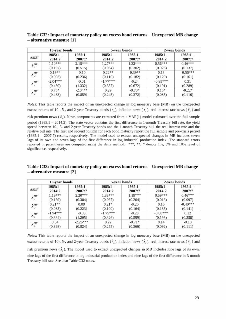
29

Table C32: Impact of monetary policy on excess bond returns – Unexpected MB change

– alternative measure [1]

10-year bonds 5-year bonds 2-year bonds

UMB 1985:1 –

2014:2

1985:1 –

2007:7 1985:1 –

2014:2

1985:1 –

2007:7

1985:1 –

2014:2

1985:1 –

2007:7

MP

nx 1.10***

(0.197)

2.15***

(0.515)

1.27***

(0.084)

1.32***

(0.302)

0.56***

(0.023)

0.46***

(0.137)

i

MP

rx

0.19**

(0.093)

-0.10

(0.236)

0.22**

(0.110)

-0.39**

(0.182)

0.18

(0.129)

-0.56***

(0.161)

MPx -2.04***

(0.430)

-0.01

(1.332)

-1.77***

(0.337)

-0.24

(0.672)

-0.89***

(0.191)

0.31

(0.289)

MP

xx 0.75*

(0.433)

-2.04**

(0.859)

0.29

(0.245)

-0.70*

(0.372)

0.15*

(0.085)

-0.22*

(0.116)

Notes: This table reports the impact of an unexpected change in log monetary base (MB) on the unexpected

excess returns of 10-, 5-, and 2-year Treasury bonds (nx ), inflation news ( x ), real interest rate news ( ir

x ) and

risk premium news (xx ). News components are extracted from a VAR(1) model estimated over the full sample

period (1985:1 – 2014:2). The state vector contains the first difference in 1-month Treasury bill rate, the yield

spread between 10-, 5- and 2-year Treasury bonds and the 1-month Treasury bill, the real interest rate and the

relative bill rate. The first and second column for each bond maturity report the full sample and pre-crisis period

(1985:1 – 2007:7) results, respectively. The model used to extract unexpected changes in MB includes seven

lags of its own and seven lags of the first difference in log industrial production index. The standard errors

reported in parentheses are computed using the delta method. ***, **, * denote 1%, 5% and 10% level of

significance, respectively.

Table C33: Impact of monetary policy on excess bond returns – Unexpected MB change

– alternative measure [2]

10-year bonds 5-year bonds 2-year bonds

UMB 1985:1 –

2014:2

1985:1 –

2007:7 1985:1 –

2014:2

1985:1 –

2007:7

1985:1 –

2014:2

1985:1 –

2007:7

MP

nx 1.19***

(0.169)

2.20***

(0.384)

1.33***

(0.067)

1.19***

(0.204)

0.59***

(0.018)

0.46***

(0.097)

i

MP

rx

0.21**

(0.085)

0.09

(0.223)

0.21*

(0.109)

-0.20

(0.164)

0.16

(0.135)

-0.40***

(0.141)

MPx -1.94***

(0.384)

-0.03

(1.205)

-1.75***

(0.326)

-0.28

(0.599)

-0.88***

(0.193)

0.12

(0.258)

MP

xx 0.54

(0.398)

-2.26***

(0.824)

0.22

(0.255)

-0.71*

(0.366)

0.14

(0.092)

-0.18

(0.111)

Notes: This table reports the impact of an unexpected change in log monetary base (MB) on the unexpected

excess returns of 10-, 5-, and 2-year Treasury bonds ( nx ), inflation news ( x ), real interest rate news ( irx ) and

risk premium news ( xx ). The model used to extract unexpected changes in MB includes nine lags of its own,

nine lags of the first difference in log industrial production index and nine lags of the first difference in 3-month

Treasury bill rate. See also Table C32 notes.

30

Table C34: Impact of monetary policy on excess bond returns – TR change

10-year bonds 5-year bonds 2-year bonds

TR 1985:1 –

2014:2

1985:1 –

2007:7 1985:1 –

2014:2

1985:1 –

2007:7

1985:1 –

2014:2

1985:1 –

2007:7

MP

nx 0.17**

(0.077)

0.31**

(0.142)

0.30***

(0.029)

0.47***

(0.067)

0.15***

(0.011)

0.22***

(0.025)

i

MP

rx

0.06**

(0.026)

-0.07

(0.058)

0.08***

(0.027)

-0.11**

(0.051)

0.08**

(0.034)

-0.16***

(0.052)

MPx -0.55***

(0.101)

0.21

(0.344)

-0.49***

(0.062)

-0.13

(0.173)

-0.28***

(0.043)

0.02

(0.085)

MP

xx 0.33**

(0.151)

-0.45**

(0.214)

0.11

(0.069)

-0.23*

(0.119)

0.05**

(0.024)

-0.08*

(0.046)

Notes: This table reports the impact of a change in log adjusted St. Louis total reserves (TR) on the unexpected

excess returns of 10-, 5-, and 2-year Treasury bonds (nx ), inflation news ( x ), real interest rate news ( ir

x ) and

risk premium news (xx ). News components are extracted from a VAR(1) model estimated over the full sample

period (1985:1 – 2014:2). The state vector contains the first difference in 1-month Treasury bill rate, the yield

spread between 10-, 5- and 2-year Treasury bonds and the 1-month Treasury bill, the real interest rate and the

relative bill rate. The first and second column for each bond maturity report the full sample and pre-crisis period

(1985:1 – 2007:7) results, respectively. The standard errors reported in parentheses are computed using the delta

method. ***, **, * denote 1%, 5% and 10% level of significance, respectively.

Table C35: Impact of monetary policy on excess bond returns – Unexpected TR change

10-year bonds 5-year bonds 2-year bonds

UTR 1985:1 –

2014:2

1985:1 –

2007:7 1985:1 –

2014:2

1985:1 –

2007:7

1985:1 –

2014:2

1985:1 –

2007:7

MP

nx 0.09**

(0.041)

0.48***

(0.103)

0.33***

(0.019)

0.34***

(0.059)

0.18***

(0.007)

0.12***

(0.024)

i

MP

rx

0.04***

(0.010)

-0.02

(0.06)

0.04

(0.023)

-0.09*

(0.051)

0.01

(0.037)

-0.14***

(0.047)

MPx -0.13***

(0.047)

0.20

(0.315)

-0.34***

(0.076)

0.00

(0.173)

-0.19***

(0.053)

0.10

(0.079)

MP

xx -0.01

(0.043)

-0.67***

(0.251)

-0.03

(0.058)

-0.26**

(0.121)

0.01

(0.027)

-0.08**

(0.038)

Notes: This table reports the impact of an unexpected change in log adjusted St. Louis total reserves (TR) on the

unexpected excess returns of 10-, 5-, and 2-year Treasury bonds (nx ), inflation news ( x ), real interest rate news

( irx ) and risk premium news (

xx ). The model used to extract unexpected changes in TR includes seven lags of

its own and seven lags of the unemployment measure as defined in Section 3.3. See also Table C34 notes.