Embed Size (px)
Citation preview
Aliased seabed detection in fisheries acoustic data
Robert Blackwell
British Antarctic Survey, High Cross, Madingley Road, Cambridge, CB3
0ET, United Kingdom
Richard Harvey
University of East Anglia, School of Computing Sciences, Norwich
Research Park, Norwich, NR4 7TJ, United Kingdom
Bastien Queste
University of East Anglia, School of Environmental Sciences, Norwich
Research Park, Norwich, NR4 7TJ, United Kingdom
Sophie Fielding
British Antarctic Survey, High Cross, Madingley Road, Cambridge, CB3
0ET, United Kingdom
April 25, 2019
Abstract
Aliased seabed echoes, also known as “false bottoms” or “shadow bottoms”, are a
form of echogram corruption caused by seabed reverberation from preceding pings
coinciding with echoes from the current ping. These aliases are usually either
avoided by adjusting the survey parameters, or identified and removed by hand - a
subjective and laborious process.
1
arX
iv:1
904.
1073
6v1
[ee
ss.S
P] 2
4 A
pr 2
019
This paper describes a simple algorithm that uses volume backscatter and split-
beam angle to detect and remove aliased seabed using single frequency, split-beam
echo sounder data without the need for bathymetry.
Keywords: acoustics; aliased seabed; echo sounder; false bottom; noise
1 Introduction
Echo sounders are routinely used in fisheries acoustics to survey marine ecosystems (Sim-
monds and MacLennan, 2008). Sound pulses (“pings”) are transmitted towards a target
and the intensity (Volume backscatter, Sv) is measured, integrated and recorded. Signals
in acoustic data come from a combination of biotic targets (e.g. fish), abiotic targets
(e.g. seabed, gas fluxes) and noise. Therefore, reflections from biological targets may be
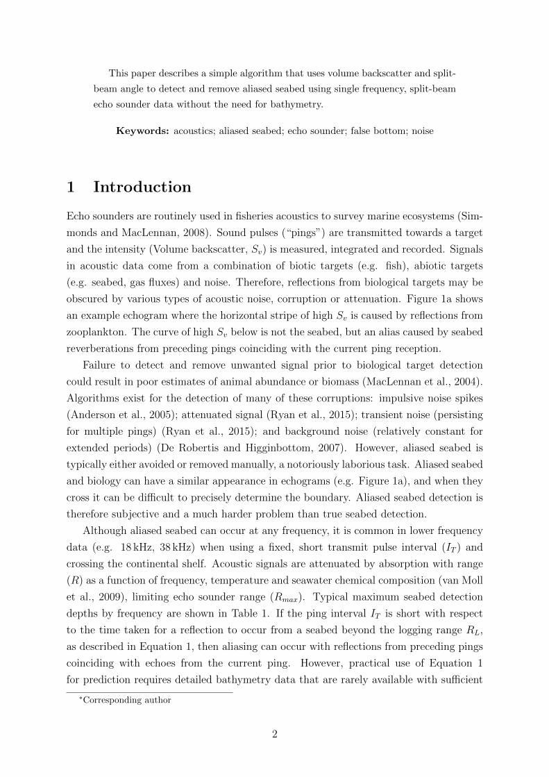
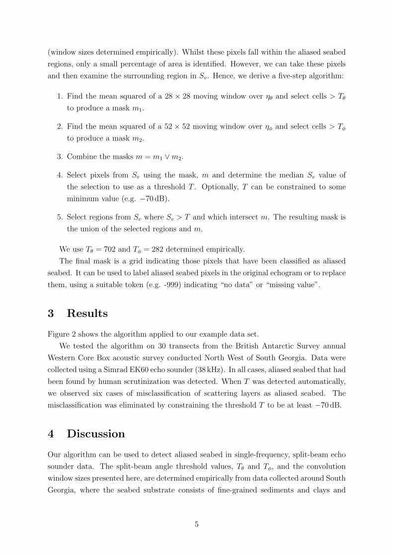
obscured by various types of acoustic noise, corruption or attenuation. Figure 1a shows
an example echogram where the horizontal stripe of high Sv is caused by reflections from
zooplankton. The curve of high Sv below is not the seabed, but an alias caused by seabed
reverberations from preceding pings coinciding with the current ping reception.
Failure to detect and remove unwanted signal prior to biological target detection
could result in poor estimates of animal abundance or biomass (MacLennan et al., 2004).
Algorithms exist for the detection of many of these corruptions: impulsive noise spikes
(Anderson et al., 2005); attenuated signal (Ryan et al., 2015); transient noise (persisting
for multiple pings) (Ryan et al., 2015); and background noise (relatively constant for
extended periods) (De Robertis and Higginbottom, 2007). However, aliased seabed is
typically either avoided or removed manually, a notoriously laborious task. Aliased seabed
and biology can have a similar appearance in echograms (e.g. Figure 1a), and when they
cross it can be difficult to precisely determine the boundary. Aliased seabed detection is
therefore subjective and a much harder problem than true seabed detection.
Although aliased seabed can occur at any frequency, it is common in lower frequency
data (e.g. 18 kHz, 38 kHz) when using a fixed, short transmit pulse interval (IT ) and
crossing the continental shelf. Acoustic signals are attenuated by absorption with range
(R) as a function of frequency, temperature and seawater chemical composition (van Moll
et al., 2009), limiting echo sounder range (Rmax). Typical maximum seabed detection
depths by frequency are shown in Table 1. If the ping interval IT is short with respect
to the time taken for a reflection to occur from a seabed beyond the logging range RL,
as described in Equation 1, then aliasing can occur with reflections from preceding pings
coinciding with echoes from the current ping. However, practical use of Equation 1
for prediction requires detailed bathymetry data that are rarely available with sufficient
∗Corresponding author
2
Figure 1: Aliased seabed echoes seen in a section of 38 kHz acoustic data with (a) volumebackscatter (Sv), (b) along-ship split beam angle (ηθ) and (c) a typical, hand-drawnaliased seabed removal mask. The horizontal axis shows pings with interval (IT ) of 2 s,nominal speed 10 kn and an extent of about 3.3 km. Data recorded using a Simrad EK60scientific echo sounder on board RRS James Clark Ross, cruise JR280.
spatial accuracy and resolution (e.g. Global Bathymetric Chart of the Oceans (IOC, 2008)
≈ 1000 m resolution, South Georgia Bathymetry Database (Hogg et al., 2016) ≈ 100 m
resolution) compared to the scale of the acoustic data (e.g. 10 m). Renfree and Demer
(2016) present the strategy for avoiding aliased seabed, by dynamically optimising IT and
the data logging range (RL). However, changing parameters mid-survey causes changes
in spatial resolution complicating subsequent data analysis. In addition, the background
noise removal method implemented by De Robertis and Higginbottom (2007) requires
a large RL to determine the noise level, thus constraining the adjustment demanded by
3
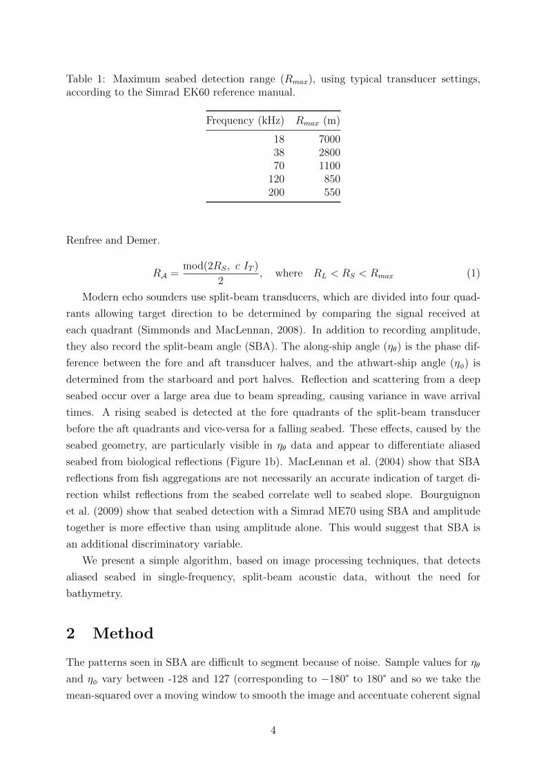
Table 1: Maximum seabed detection range (Rmax), using typical transducer settings,according to the Simrad EK60 reference manual.
Frequency (kHz) Rmax (m)
18 700038 280070 1100
120 850200 550
Renfree and Demer.
RA =mod(2RS, c IT )
2, where RL < RS < Rmax (1)
Modern echo sounders use split-beam transducers, which are divided into four quad-
rants allowing target direction to be determined by comparing the signal received at
each quadrant (Simmonds and MacLennan, 2008). In addition to recording amplitude,
they also record the split-beam angle (SBA). The along-ship angle (ηθ) is the phase dif-
ference between the fore and aft transducer halves, and the athwart-ship angle (ηφ) is
determined from the starboard and port halves. Reflection and scattering from a deep
seabed occur over a large area due to beam spreading, causing variance in wave arrival
times. A rising seabed is detected at the fore quadrants of the split-beam transducer
before the aft quadrants and vice-versa for a falling seabed. These effects, caused by the
seabed geometry, are particularly visible in ηθ data and appear to differentiate aliased
seabed from biological reflections (Figure 1b). MacLennan et al. (2004) show that SBA
reflections from fish aggregations are not necessarily an accurate indication of target di-
rection whilst reflections from the seabed correlate well to seabed slope. Bourguignon
et al. (2009) show that seabed detection with a Simrad ME70 using SBA and amplitude
together is more effective than using amplitude alone. This would suggest that SBA is
an additional discriminatory variable.
We present a simple algorithm, based on image processing techniques, that detects
aliased seabed in single-frequency, split-beam acoustic data, without the need for
bathymetry.
2 Method
The patterns seen in SBA are difficult to segment because of noise. Sample values for ηθ
and ηφ vary between -128 and 127 (corresponding to −180° to 180° and so we take the
mean-squared over a moving window to smooth the image and accentuate coherent signal
4
(window sizes determined empirically). Whilst these pixels fall within the aliased seabed
regions, only a small percentage of area is identified. However, we can take these pixels
and then examine the surrounding region in Sv. Hence, we derive a five-step algorithm:
1. Find the mean squared of a 28 × 28 moving window over ηθ and select cells > Tθ
to produce a mask m1.
2. Find the mean squared of a 52 × 52 moving window over ηφ and select cells > Tφ
to produce a mask m2.
3. Combine the masks m = m1 ∨m2.
4. Select pixels from Sv using the mask, m and determine the median Sv value of
the selection to use as a threshold T . Optionally, T can be constrained to some
minimum value (e.g. −70 dB).
5. Select regions from Sv where Sv > T and which intersect m. The resulting mask is
the union of the selected regions and m.
We use Tθ = 702 and Tφ = 282 determined empirically.
The final mask is a grid indicating those pixels that have been classified as aliased
seabed. It can be used to label aliased seabed pixels in the original echogram or to replace
them, using a suitable token (e.g. -999) indicating “no data” or “missing value”.
3 Results
Figure 2 shows the algorithm applied to our example data set.
We tested the algorithm on 30 transects from the British Antarctic Survey annual
Western Core Box acoustic survey conducted North West of South Georgia. Data were
collected using a Simrad EK60 echo sounder (38 kHz). In all cases, aliased seabed that had
been found by human scrutinization was detected. When T was detected automatically,
we observed six cases of misclassification of scattering layers as aliased seabed. The
misclassification was eliminated by constraining the threshold T to be at least −70 dB.
4 Discussion
Our algorithm can be used to detect aliased seabed in single-frequency, split-beam echo
sounder data. The split-beam angle threshold values, Tθ and Tφ, and the convolution
window sizes presented here, are determined empirically from data collected around South
Georgia, where the seabed substrate consists of fine-grained sediments and clays and
5
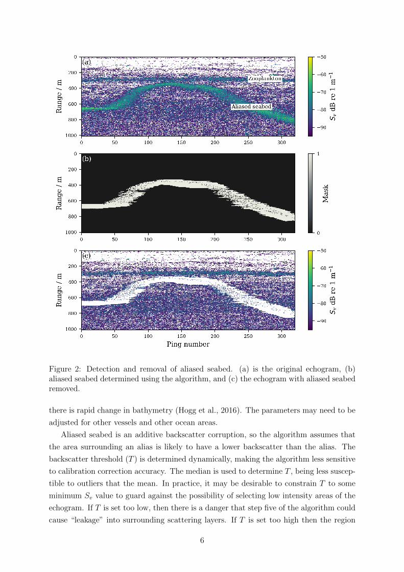
Figure 2: Detection and removal of aliased seabed. (a) is the original echogram, (b)aliased seabed determined using the algorithm, and (c) the echogram with aliased seabedremoved.
there is rapid change in bathymetry (Hogg et al., 2016). The parameters may need to be
adjusted for other vessels and other ocean areas.
Aliased seabed is an additive backscatter corruption, so the algorithm assumes that
the area surrounding an alias is likely to have a lower backscatter than the alias. The
backscatter threshold (T ) is determined dynamically, making the algorithm less sensitive
to calibration correction accuracy. The median is used to determine T , being less suscep-
tible to outliers that the mean. In practice, it may be desirable to constrain T to some
minimum Sv value to guard against the possibility of selecting low intensity areas of the
echogram. If T is set too low, then there is a danger that step five of the algorithm could
cause “leakage” into surrounding scattering layers. If T is set too high then the region
6
of aliased seabed detected is reduced in size. Minimum T should therefore be adjusted
based on observed results.
Speckle is seen in some aliased seabed detections (Figure 2b). This can be removed
using a hole filling image processing algorithm (e.g. morphological reconstruction (Soille,
2013), as used by Matlab imfill). Visual inspection of echograms shows that our auto-
mated results find several instances of aliased seabed that had not been identified man-
ually. On further inspection these appear to be genuine and, in some cases, are fainter
aliases caused by the echoes from antepenultimate pings.
Our algorithm is simple to implement and efficient in terms of computational re-
sources. The windowing operations can be implemented using two-dimensional convolu-
tion which is fast on modern hardware (the example in Figure 2 takes about 0.43 s on
a 2016 Intel Skylake i7 processor). Whilst the algorithm does not rely on other noise
removal strategies beyond true seabed removal, its performance can reduce if the data
include impulse noise, transient noise or attenuated signal. In these cases, the methods
described by Anderson et al. (2005) and Ryan et al. (2015), combined with interpolation
(e.g. median filtering) to replace the noise, are an effective preprocessing step. If using
background noise removal (e.g. De Robertis and Higginbottom (2007)), we recommend
implementing this after aliased seabed detection.
We want our method to be independent of ping interval (IT ) and logging range (RL),
and so we choose to use a single frequency. We are also interested in using data from ships
of opportunity (e.g. fishing vessels) which may only have a single frequency. However, If
multi-frequency data are available then, depending on maximum range (Rmax) and seabed
depth (RS), other frequencies can be used to further validate aliased seabed. (E.g. if
an aliased seabed candidate was observed at 500 m in 38 kHz data, with ping interval
IT = 2 s then, using Equation 1, seabed depth RS = 2000 m. If a corresponding signal
was seen in 70 kHz data, then the maximum range (Rmax) would be insufficient to reach
the seabed, and so the signal must have another cause). Lower frequency data could allow
RS to be detected automatically and allow the methods of Renfree and Demer (2016) to
be used as part of a hybrid approach. A consequence of Equation 1 is that RS ≮ RL
and so aliased seabed cannot occur in a ping where the true seabed has already been
detected.
Using split-beam angle in addition to volume backscatter is known to improve bottom
detection (MacLennan et al., 2004; Bourguignon et al., 2009). Large coherent patterns
in SBA are a strong indication of reflections from the seabed, but not biology. We
extend this observation to aliased seabed and use it to create an automated algorithm
providing consistent, repeatable results. We have tested the algorithm with Simrad EK60
data, which uses a four quadrant, split-beam configuration. Some new transducers use
a three-sector design, however we expect the principles to be transferable. Although we
designed the algorithm for aliased seabed detection, mutatis mutandis, it may also have
7
applications as a bottom detector.
5 Conclusions
The method we describe is intended to make aliased seabed detection and removal semi-
automatic, fast and reproducible. It could be incorporated into existing tooling to reduce
the labour required to clean fisheries acoustic data. We recommend that practitioners
check results using visual inspection.
Acknowledgements
Our thanks to the officers, crew and scientists onboard the RRS James Clark Ross and
RRS Discovery for their assistance in collecting the data.
Alejandro Ariza (British Antarctic Survey) provided helpful insight into the problems
caused by aliased seabed.
The Western Core Box cruises and SF are funded as part of the Ecosystems Pro-
gramme at the British Antarctic Survey, Natural Environment Research Council, a part
of UK Research and Innovation.
This work was supported by the Natural Environment Research Council grant
NE/N012070/1.
References
Anderson, C., Brierley, A., and Armstrong, F. (2005). Spatio-temporal variability in the
distribution of epi-and meso-pelagic acoustic backscatter in the Irminger Sea, North
Atlantic, with implications for predation on Calanus finmarchicus. Marine Biology,
146(6):1177–1188.
Bourguignon, S., Berger, L., Scalabrin, C., Fablet, R., and Mazauric, V. (2009). Method-
ological developments for improved bottom detection with the ME70 multibeam
echosounder. ICES Journal of Marine Science: Journal du Conseil, 66(6):1015–1022.
De Robertis, A. and Higginbottom, I. (2007). A post-processing technique to estimate
the signal-to-noise ratio and remove echosounder background noise. ICES Journal of
Marine Science: Journal du Conseil, 64(6):1282–1291.
Hogg, O. T., Huvenne, V. A., Griffiths, H. J., Dorschel, B., and Linse, K. (2016). Land-
scape mapping at sub-Antarctic South Georgia provides a protocol for underpinning
large-scale marine protected areas. Scientific reports, 6.
8
IOC, I. (2008). BODC, 2003. Centenary Edition of the GEBCO Digital Atlas, published
on CD-ROM on behalf of the Intergovernmental Oceanographic Commission and the
International Hydrographic Organization as part of the General Bathymetric Chart of
the Oceans. British Oceanographic Data Centre, Liverpool, UK, 260.
MacLennan, D., Copland, P., Armstrong, E., and Simmonds, E. (2004). Experiments
on the discrimination of fish and seabed echoes. ICES Journal of Marine Science,
61(2):201–210.
Renfree, J. S. and Demer, D. A. (2016). Optimizing transmit interval and logging range
while avoiding aliased seabed echoes. ICES Journal of Marine Science, 73(8):1955–
1964.
Ryan, T. E., Downie, R. A., Kloser, R. J., and Keith, G. (2015). Reducing bias due to
noise and attenuation in open-ocean echo integration data. ICES Journal of Marine
Science: Journal du Conseil, 72(8):2482–2493.
Simmonds, J. and MacLennan, D. N. (2008). Fisheries acoustics: theory and practice.
John Wiley & Sons.
Soille, P. (2013). Morphological image analysis: principles and applications. Springer
Science & Business Media.
van Moll, C. A., Ainslie, M. A., and van Vossen, R. (2009). A simple and accurate
formula for the absorption of sound in seawater. IEEE Journal of Oceanic Engineering,
34(4):610–616.
9