International fisheries agreements with a shifting stock∗

Florian K Diekert† Emmi Nieminen‡

July 2015

Abstract

When a fish stock shifts from one nation to another nation, e.g. due to climate change,

the nation that loses the resource has incentives to deplete it while the other nation,

receiving the resource, has incentives to conserve it. We propose an analytical model

to study under which circumstances self-enforcing agreements can align incentives.

Our setup allows to distinguish between a fast and a slow shift in ownership and be-

tween a smooth or a sudden shift. We show that the shorter the expected duration of

the shift, the higher the total equilibrium exploitation rate. Similarly, a sudden shift

implies – by and large – more aggressive non-cooperative exploitation than a gradual

transition. However, a self-enforcing agreement without side-payments is more likely

for a sudden than for a smooth shift. Further, the scope for cooperation increases

with the expected duration of the transition, and it decreases with the renewability

of the resource and the discount rate. Most importantly, we show that concentrating

on in-kind transfers can be very detrimental for shifting renewable resources: In some

cases, no efficient bargaining solution exists, even when there are only two players.

Keywords: Renewable Resources; Dynamic Game; International Environmental Agree-

ments; Regime Shift; Climate Change.

JEL Codes: C73, Q22, Q54

1 Introduction

Climate change will put existing International Fisheries Agreements under severe stress

(Miller et al., 2013). In fact, this is already happening today. For example, the appearance

of Atlantic mackerel in Icelandic waters has brought Iceland, Faroese, Norway and the EU

∗This research is funded by NorMER, a Nordic Centre of Excellence for Research on Marine Ecosystemsand Resources under Climate Change. We would like to thank Chris Costello, Rognvaldur Hannesson,Marko Lindroos, and seminar participants at UCSB, the 2014 IIFET conference in Brisbane, and the 2014Annual NorMER meeting in Copenhagen for their constructive comments and feedback. All remainingerrors are, of course, our own.†Department of Economics and CEES, Department of Biosciences. University of Oslo, PO-Box 1095,

Blindern, 3017 Oslo, Norway. E-mail: f.k.diekert@ibv.uio.no.‡Department of Economics and Management. University of Helsinki, PO-Box 27, 00014 University of

Helsinki, Finland. E-mail: emmi.e.nieminen@helsinki.fi

1

to the brink of a new “fish war”. The previous fisheries agreement has collapsed and the

conflict over the level and distribution of fish quotas has – to date – not been resolved.

Similarly, salmon stocks along the West Coast of Canada and the US have shifted their

distribution depending on the climatic regime. This has repeatedly led to a break-down

of the US-Canadian agreement on the Pacific salmon fisheries.

In this paper, we develop a dynamic non-cooperative game where the ownership of

a productive resource shifts from one player to the other at an uncertain point in time.

Contrary to the benchmark game of joint ownership but no shift, it is not always possible

to achieve a stable, mutually beneficial, sharing agreement – even when there are only two

players. A shifting distribution increases the bargaining position of the party whose share

of the resource increases, while it decreases the bargaining strength of the other party.

The first party thus wants to re-negotiate to obtain a more favorable agreement: The

party receiving the resource stock will have more conservation incentives than the party

losing the resource. Consider a pie which can be eaten exclusively by player A in the first

period, and whatever player A leaves on the plate will be owned by player B in the second

period. Abstracting from discounting or uncertainty, player A’s optimal strategy is to eat

the entire pie in the first period. Without side-payments, there is no contract that player

B could offer player A to make both strictly better off.

When the asset can be liquidated, or more generally transfers in utility are permitted,

this tension is resolved immediately. The former party simply buys out the latter party.

That is, player B can just pay player A the amount that is equivalent to eating half the

pie in exchange for leaving half of it for the second period. In essence, the Coase-Theorem

tells us that the allocation of initial property rights should not matter for the possibility

to achieve an efficient bargaining solution. We show that this reasoning does not hold in

a dynamic context when transfers are to be made in-kind.

Concentrating on in-kind transfers is particularly relevant for natural resources. For

simple technological reasons, it may not be possible to liquidate fish stocks or forests in the

same way as financial assets. More importantly, however, questions of national sovereignty,

political legitimacy, and ethical concerns play an important role in this context. Quite

generally, it is natural to restrict attention to in-kind transfers in a dynamic, intergener-

ational, setting. Future generations are simply not around to share the potential surplus

from an efficient transfer of the resource with the current generation.

This is not to say that an analysis of financial side-payments is not interesting per se.

Munro (1979) has pointed out more than 30 years ago that financial side-payments (or

equivalently: direct profit-sharing) may greatly ease the prospects of attaining a cooper-

ative solution – though the issue of time-consistency remains (Vislie, 1987). Relatedly,

Costello and Kaffine (2011) show that unitization of a spatially connected renewable re-

source can yield the first-best outcome as a sub-game perfect equilibrium under profit-

sharing, but not under revenue-sharing. Indeed, profit sharing or financial side-payments

are rarely observed in practice. Of course, the fact that one does not see a blunt state-

ment such as “you receive x dollar for each ton of fish that I am allowed to harvest in your

waters” does not mean that there are not more subtle ways of side-payments via issue-

2

linkage in multi-layered international negotiations. Nevertheless, we argue that the scope

of financial side-payments to enable international agreements is limited, especially when

the utility derived from fishing captures broader aspects than just profits, such as cultural

identity, tourism, employment, etc. It is politically, and to some extent also ethically,

difficult to express these aspects in monetary terms.

We build on the “fish war” framework of Levhari and Mirman (1980) to develop

a tractable model of an international fishery that is shared between two nations, and

where the fish stock shifts from one player to the other. We solve for the feedback

Nash-equilibrium of the dynamic non-cooperative game and characterize the scope of

self-enforcing agreements to divide the optimal harvest share. Moreover, we explicitly

consider different types of transition dynamics: Is non-cooperative exploitation more ag-

gressive when the change in ownership occurs suddenly or gradually? Can cooperation

more easily be achieved when the change in ownership is fast, or when it is slow?

Relation to the literature

The breakdown of the Coase Theorem in a dynamic setting without commitment is most

prominently discussed in the literature on political economics (Dixit et al., 2000; Acemoglu,

2003). Recently, Harstad (2013) has applied these insights to environmental goods. In his

setup, the owner, or the seller, of a “conservation good” (such as a tropical forest) desires

to consume it, but the buyer benefits more from conservation. However, the buyer is also

satisfied when the good is not consumed, and thus it has an existence value to the buyer.

Contradictorily, the buyer is not willing to pay when the seller is conserving the good, and

the seller is conserving only if the buyer is expected to buy, leading to the conclusion that

a “market for conservation” is unlikely to exist.

Our paper adds to this by explicitly dealing with a dynamic renewable resource. It is

thereby related to two strands of literature. First of all, it ties to the theoretical work on

self-enforcing agreements over renewable resources. Using the Levhari-Mirman framework

as we do, Kwon (2006) studies the existence of self-enforcing coalitions, finding – as it

is common in the international agreements literature (Barrett, 1994) – that coalitions of

more than two or three players are generally not stable. Using “farsighted” instead of

Nash conjectures, Breton and Keoula (2012) derive less pessimistic results: Cooperation

can be sustained under a much larger range of circumstances because threats of successive

deviations are credible when players anticipate the formation of new coalition structures.

Considering asymmetric players, however, does not yield similarly optimistic outcomes

with respect to the size of stable coalitions (Breton and Keoula, 2014). Fesselmeyer and

Santugini (2013) do not study coalition structures, but the exogenous risk of regime shifts

in the “fish war” model, arguing that a negative shock may exacerbate the inefficiency

implied by non-cooperation. Miller and Nkuiya (2014) then show that the threat of a

negative regime shift may actually induce more cooperation and allow larger coalition

sizes. We differ from the above contributions by considering a structurally asymmetric

setup: The resource shifts from player A to B, and while the shared ownership induces

3

efficiency losses, it is the fact that A loses the resource which hinders the formation of

international agreements.

Therefore, our paper is also related to the literature on expropriation in the context of

natural resources (Long, 1975; Ryszka, 2013). In our case, the rapacity effects of excessive

resource depletion are not induced by exogenous expropriation risk, but by a combination

of a regime shift risk with the presence of another strategic player.

Finally, we add to the growing body of research that specifically deals with the effects

of climate change on international fisheries agreements. The first paper addressing in this

line is from McKelvey et al. (2003), who argue that altered habitat or migration routes

may destabilize existing agreements. The authors therefore argue for flexible quota shares.

As we show here, flexible quota sharing certainly is important, but it may actually not be

enough to avoid undesired competition. The model of McKelvey et al. (2003), which is

an extension of the classical fish-war model of Levhari and Mirman (1980), is now known

as the “split-stream model” and forms the basis of several papers: Liu et al. (2012) con-

sider the distribution of the Norwegian spring-spawning herring and study partial coalition

structures. They conclude that cost asymmetry improves the stability of the grand coali-

tion, and non-cooperation gives more conservation incentives to the major player than the

minor player. Liu and Heino (2013) compare proactive management that takes possible

climate change effects on the stock distribution into account with reactive management.

They find that the players behave symmetrically under reactive management, but proac-

tive management encourages the player losing the stock to act more aggressively. They

conclude that the stock will be in greatest danger when both players own equal shares,

confirming theoretical work of Hannesson (2007). Hannesson (2007) further points out

that the transition of ownership may even lead to an extinction of the stock when harvest-

ing costs are independent of the stock. The Northeast Atlantic mackerel stock is studied

by Hannesson (2013) under three different hypothesis about what causes the shift in stock

distribution. He concludes that the minor player has a stronger bargaining position when

the migration pattern is deterministic or purely random. Under a stock-dependent migra-

tion, the major player has a threat strategy to fish down the stock to such a low level that

it does not spill over to the minor player’s zone. Another recent application to the same

stock is Ellefsen (2013), confirming that the agreement is destabilized by a new entrant,

and that it is the major player who has to pay most in order to encourage the new member

to join. Because we go back to the “fish war” predecessor of the “split-stream model”, we

can derive explicit analytical solutions to the feedback equilibrium instead of relying on

numerical simulations, or confining our discussion to steady-state outcomes.

2 The Model

Consider a situation with two neighbouring nations, A and B, that derive utility from

harvesting fish from a stock whose size at time t is given by xt. However, a nation’s access

to this resource may be limited, for example because the majority of the fish stock is

outside the countries’ exclusive economic zone (EEZ), or because one nation has specialized

4

in harvesting a sub-population. Specifically, let st be the share of the stock that country A

can access (due to technology or politics). Correspondingly, 1− st of the stock is “owned”

by player B. Global warming (or some other form of environmental change) is expected

to alter the distribution of the fish stock. Specifically, we will assume that, in any period,

the players’ share remains the same with probability q, and with probability 1− q, there

will be a shift in the distribution of the fish stock. We will generally presume that the

stock moves from player A to player B. That is, the share st, that player A has access to,

is expected to decline with time. Correspondingly, player B expects to see an increase in

the part of the resource that he can harvest.

There are several real-world cases that fit this generic description. For example, At-

lantic Mackerel was basically absent from Icelandic waters and this fish stock was almost

exclusively harvested by Norway and the European Union in the past. However, since

2006/07 more and more of the fish is found in Icelandic waters (Hannesson, 2013). It is

yet to be seen whether stock shares will stabilize at the current levels, or whether the

change continues so that the stock will eventually leave the Norwegian and European wa-

ters altogether. While access to the stock has a clear geographic/political interpretation

in the former example, it could also have a technological interpretation. In the Baltic Sea,

pelagic and demersal fisheries have always coexisted to some extent. Originally, the food

web was dominated by cod, which was heavily fished. In the late 1980s, a rapid regime

shift occurred and the system has since been dominated by small planktivorous fishes such

as sprat (Casini et al., 2012). Recent research indicates that this change is likely to be

permanent (Blenckner et al., 2015). When interpreting xt not as the stock of a specific

species, but more broadly as the productive potential of an ecosystem, one can clearly

say that the share of the resource s, that is available for fishing firms that specialize on

catching cod, has declined dramatically, whereas the resource share has increased for those

firms that have invested in gear to target small pelagics.

In this section, we will present the basic setup of our model and characterize the non-

cooperative equilibrium. In section 3, we discuss the scope for self-enforcing agreements,

and in section 4, we explore differences in the quality of the shift (i.e. whether it is slow

or fast, gradual or smooth).

The basic setup

We build on the classical model by Levhari and Mirman (1980) with two players that

apply the same discount factor β. Time is discrete with t = 0, 1, 2, ... Players derive utility

from consuming the resource according to u(cit) = ln(cit), where i = A,B. It is well known

that this game has a unique Nash equilibrium in linear strategies (Long, 2010), and we

will therefore concentrate on linear strategies. To simplify notation, we denote player

A’s extraction rate by at and player B’s extraction rate by bt (so that cAt = atxt and

cBt = btxt). Denote the total extraction rate by dt (so that dt ≡ at + bt). The resource

5

develops according to:

xt+1 = M ((1− dt)xt)α (1)

The parameter α determines the “renewability” of the resource with α ∈ (0, 1) and the

smaller is α, the stronger is the natural re-growth potential of the resource. M is a scaling

parameter which has no effect on the optimal choice of the extraction rate. It ensures that

the value-function of the players remains non-negative in all stages of the game.1 For a

constant exploitation rate d, the steady-state value of x is given by x = M ((1− d)M)α

1−α .

To allow for a general analysis of the effect of an anticipated, but uncertain shift

in ownership, we assume that the transition of the resource from player A to player B

proceeds in stages. In total, there are T stages, and within each stage τ (where τ =

0, 1, ...T ) the share of the stock that player A has access to is given by sτ and the share

of the stock that player B has access to is given by 1 − sτ . In other words, the player’s

harvesting rates in a given stage τ are constrained by aτ ≤ sτ and bτ ≤ 1 − sτ . The

duration of each stage is unknown, but there is a constant probability q that the systems

stays in the current stage and there is a constant probability 1 − q that after any given

period the next period starts in a new stage with sτ+1. We assume that s0 = 1 and

sT = 0. and we require that sτ < sτ+1. Other than that, we do not need to impose

further restrictions on the way how the resource changes ownership. Note however, that

the assumption that sT = 0 is not innocuous. It means that player A completely loses

her access to the resource, and that her time horizon is essentially finite (although it is

uncertain when the end arrives).

It can be shown that when sT is larger than zero, no matter how small sT is, one

would end up in a situation that is essentially the same as the standard Levhari-Mirman

game. Structurally, the reason is that the marginal utility of consumption grows without

bounds as c → 0 when using a logarithmic utility function. We argue that this feature

of the model does not have a meaningful interpretation in the case of real world fisheries.

Rather, we understand our model so that when s has dropped below some level, it does no

longer pass the cost-benefit test to continue harvesting from this resource and the fishery

is abandoned. (Recall that we scale the parameter M so that the value of active harvesting

is always positive).

General pattern of the non-cooperative equilibrium

For a given share of the resource, sτ , and a given size of the stock xt, player A (or player B

for that matter) maximizes utility from consuming a share of the resource now and in the

future. The player takes into account that with probability q, the environmental regime

will stay the same. Thus, the future value of the game, conditional on stock development,

is the same as today. Denote this value by V A(sτ , xt). With probability 1 − q, however,

1Let imin be the lowest extraction rate of player i and let dmax be the largest equilibrium to-tal extraction rate. Then a condition that guarantees non-negative objective function values isiminM ((1− dmax)M)

α1−α ≥ 1 for i = A,B.

6

the environmental regime will change to the next stage and the value of the game is then

given by V A(sτ+1, xt+1). In other words, there are two dynamic dimensions and two state

variables in this game. Namely, (calendar) time t and the index τ that counts which stage

the game is in. The resource stock xt moves with calendar time, but the way the resource

is shared (given by sτ ) changes from stage to stage. Note that although the overall game

is not stationary, the problem that the players face at any point in time is stationary.

Player A’s and B’s value functions are therefore given by:

V A(sτ , xt) = maxa≤sτ

{ln axt + β

[qV A(sτ , xt+1) + (1− q)V A(sτ+1, xt+1)

]}(2)

V B(sτ , xt) = maxb≤1−sτ

{ln bxt + β

[qV B(sτ , xt+1) + (1− q)V B(sτ+1, xt+1)

]}(3)

As it is usual in “fish war” models, we suspect that also here, the player’s value function

is of the log-linear form V i(sτ , xt) = kiτ lnxt + Kiτ for i = A,B. This conjecture leads to

the following first-order condition for player A:

1

aτ= αβqkAτ

1

1− aτ − bτ+ αβ(1− q)kAτ+1

1

1− aτ − bτ

Accordingly, we can solve for player A’s best-reply. Noting that her extraction can be

limited by the accessible share sτ , we have:

aτ = min

{sτ ;

(1− bτ )

1 + αβ(qkAτ + (1− q)kAτ+1)

}(4)

The general case of player B is symmetric, and hence his best-reply is:

bτ = min

{1− sτ ;

(1− aτ )

1 + αβ(qkBτ + (1− q)kBτ+1)

}(5)

We now set out to derive the structure of the coefficients kiτ and Kiτ . Noting that the

structure is the same for player A and B, we equate coefficients generically (where jτ = aτ

if i = A and jτ = bτ if i = B):

kiτ lnx+Kiτ = ln jτx+ αβq

[kiτ

(ln(1− aτ − bτ )x+

1

αlnM

)+

1

αKiτ

]+ αβ(1− q)

[kiτ+1

(ln(1− aτ − bτ )x+

1

αlnM

)+

1

αKiτ+1

]⇒

kiτ =1

1− αβq+αβ(1− q)1− αβq

kiτ+1 (6)

7

This linear difference equation with constant coefficients can be solved2 to give:

kiτ =

(αβ(1− q)1− αβq

)T−τ [kiT −

1

1− αβ

]+

1

1− αβ(7)

Note that the solution of kiτ will depend on kiT , which – in turn – depends on the utility

derived from fishing in the last stage.

Player A’s value of the fishery will be zero in the last stage (sT = 0), so that we

have kAT = 0. This implies that kAτ = 11−αβ

(1−

(αβ(1−q)1−αβq

)T−τ). It is easy to see that

kAτ > kAτ+1: The term in the first bracket is smaller than one (as both αβ < 1 and q < 1

and therefore αβ − αβq < 1 − αβq), and the first term will therefore decrease as the

exponent gets larger. In the beginning, kAτ will be close to the steady-state value of (7),1

1−αβ , especially when T is large. For player B, we have kBτ = 11−αβ for all τ .

Although the coefficients KAτ and KB

τ are irrelevant for the choice of the harvesting

rate, we do need to spell them out in order to fully describe the value functions later on.

Kiτ =

1

1− βq[ln jτ + β

((1− q)Ki

τ+1 + (qkiτ + (1− q)kiτ+1)(lnM + α ln(1− dτ ))]

(8)

Equation (8), in contrast to (6), is a difference equation where the coefficients are not

constant, nor necessarily the same for both players. Solving it is therefore not instructive.

To describe the general pattern of the equilibrium in a concise form, we introduce the

following auxiliary parameter:

γiτ ≡1

1 + αβ[qkiτ + (1− q)kiτ+1]where γBτ = γB = (1− αβ) (9)

Although the game is stationary within each stage, the extraction rates differ from

stage to stage as summarized in the following proposition.

Proposition 1. The extraction pattern is characterized by at most three phases:

I. When sτ ∈ [1, 1 − bτ ), player B’s extraction rate is constrained by the share of the

resource available to him, while player A’s rate is not. Total extraction rate dτ is

increasing with τ in Phase I. The individual extraction rates are given by:

aτ = sτγAτ bτ = 1− sτ (10)

II. When sτ ∈ [1 − bτ , aτ ], neither player’s extraction rate is constrained. Player A’s

extraction rate is increasing and player B’s extraction rate is decreasing with τ , and

2We refer to a standard mathematic textbook for economists e.g. Sydsæter et al. (2005, p.391). To seethe solution more clearly, it is useful to change variables so that we start counting from the terminal stageT . That is, we introduce a new variable n = 0, 1, 2, ... so that n = 0 ≡ τ = T . This means that equation (6)is written as: kin+1 = l+mkin which can be solved to get kin = mnk0 + l(

∑(mn)). As we have a geometric

series in the brackets, the solution of the equation can be rewritten as: kin = l(1−mn)1−m + mk0 ⇔ kin =

mn[k0 − l1−m ] + l

1−m , where l1−m = 1

1−αβq1

1−αβ(1−q)1−αβq

= 11−αβq

1(1−αβq)−αβ(1−q)

1−αβq= 1

1−αβq−αβ+αβq = 11−αβ .

8

the total extraction rate is increasing, where:

aτ =γAτ (1− γB)

1− γAτ γBbτ =

γB(1− γAτ )

1− γAτ γB(11)

III. When sτ ∈ (aτ , 0], the extraction rate of player A, but not player B is constrained by

the available share of the resource. Total extraction rate is decreasing with τ .

aτ = sτ bτ = (1− sτ )γB (12)

Proof. The proof is given in Appendix A.1. Note that extraction is indeed linear in x in

all cases, so that the conjecture about the form of the value function is confirmed.

3 Self-enforcing cooperative agreements

In this section, we explore whether the players can agree on sharing the gains from max-

imizing the joint surplus of resource exploitation. It is well known that self-enforcing

cooperative agreements of more than a few players are very difficult to form (Kwon, 2006;

Breton and Keoula, 2014). Here we show that even two players may not be able to coor-

dinate on the first-best if the stock shifts from one player to the other.

As we focus on in-kind transfers (ruling out financial side-payments), we ask whether

the optimal total harvest can be split in such a way that each player’s participation

constraint – which is given by his payoff in absence of cooperation – is satisfied. In other

words, we analyze whether there exists some share λ so that player A prefers obtaining

that share of the socially optimal harvest rather than harvesting non-cooperatively, and

whether player B would at the same time prefer obtaining a share (1 − λ) rather than

harvesting non-cooperatively. That is, we assume that at any time t, the players perceive

the Nash equilibrium described above as the only alternative to a cooperative agreement

for that stage. In essence, the players follow a grim trigger strategy within each stage.

We do not require that the threat of non-cooperative play is renegotiation-proof. Such

an agreement is self-enforcing in the sense that player A has no incentive to harvest non-

cooperatively, given that player B harvests cooperatively, and vice-versa.

To clearly distinguish the different continuation values, we denote the player’s value

function in the non-cooperative Nash equilibrium at stage τ by V nc,iτ (sτ , xt). In contrast,

V coop,iτ (λ, xt) describes the value of cooperation for player i, given the share λ and the cur-

rent resource stock xt. Let V iτ ≡ max{V coop,A

τ , V nc,Aτ (xt)}, so that the function V i

τ+1(xt+1)

is generic value of the game in the next stage (where it is a priori not known whether

cooperative or non-cooperative play will dominate). Denoting the socially optimal total

9

harvest rate by d∗, we can write:

V coop,Aτ (λ, xt) = ln (λd∗xt) + β

(qV coop,A

τ (λ, xt+1) + (1− q)V Aτ+1(xt+1)

)V coop,Bτ (λ, xt) = ln ((1− λ)d∗xt) + β

(qV coop,B

τ (λ, xt+1) + (1− q)V Bτ+1(xt+1)

)Below, we show that reaching a cooperative agreement in any given stage τ does

not depend on whether an agreement can be reached in the next stage. Changes in the

external conditions may, in accordance with public international law3, make the current

treaty inapplicable and will in fact often lead to re-negotiations of existing agreements.

Therefore, in any given stage τ , a cooperative agreement can be reached for that stage if

condition (13) holds for any value of xt.

V coop,Aτ (λ, xt) ≥ V nc,A

τ (xt) and V coop,Bτ (λ, xt) ≥ V nc,B

τ (xt) (13)

Clearly, V coop,Aτ (λ, xt) is increasing in λ and V coop,B

τ (λ, xt) is decreasing in λ. Let

therefore λAmin ∈ (0, 1] be the minimum share of the optimal harvest that player A would be

willing to accept in order to approve cooperative management. Similarly, let λBmax ∈ (0, 1]

the maximum share that player B would be willing to give to player A and still harvest

cooperatively. Accordingly, we can define the scope for cooperation by:

Γ ≡{λBmax − λAmin; 0

}(14)

This allows us to state the following proposition:

Proposition 2. Cooperation possibilities are not constrained by the available harvest

shares, but the scope for cooperation vanishes as q → 0 or αβ → 1. If there is scope

for cooperation (Γ > 0), λAmin and λBmax are given by equation (15) and (16), respectively

(where ϕAτ = qkAτ + (1− q)kAτ+1 and ϕB = 11−αβ ).

λAmin =aτ

1− αβ

(1− aτ − bτ

αβ

)αβϕAτ(15)

λBmax = 1− bτ1− αβ

(1− aτ − bτ

αβ

)αβϕB(16)

Proof. The proof is given in Appendix A.2.

Intuition can be built by considering the following simple example, which effectively

sets q = 0 and αβ = 1: There are only two periods, the resource is completely non-

renewable, and player A, who owns the resource entirely in the first period, will for sure

3The legal principle that treaties must be honoured (pacta sunt servanda) is understood to be contingenton the current state of affairs when the treaty was made (rebus sic stantibus).

10

lose it in the next period. Even without discounting, player A has no incentive to leave

anything for player B. In fact, as A’s best-reply is to consume the entire resource, there

is no share that player B can offer player A to make both strictly better off.

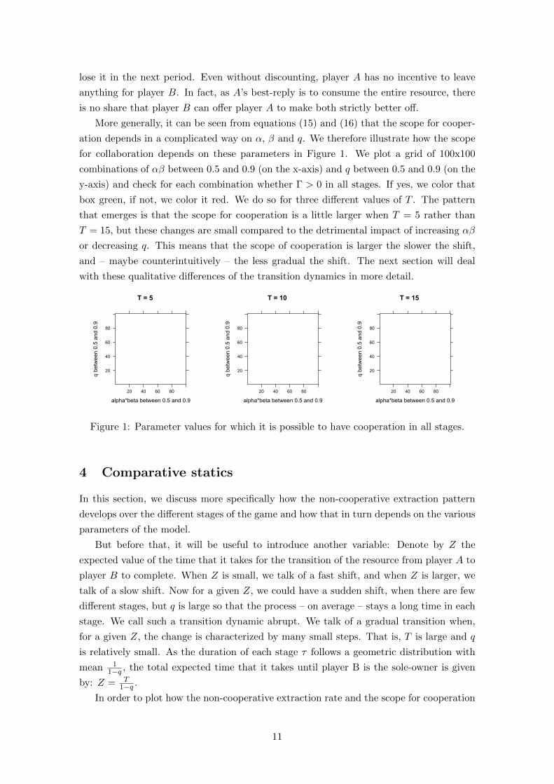
More generally, it can be seen from equations (15) and (16) that the scope for cooper-

ation depends in a complicated way on α, β and q. We therefore illustrate how the scope

for collaboration depends on these parameters in Figure 1. We plot a grid of 100x100

combinations of αβ between 0.5 and 0.9 (on the x-axis) and q between 0.5 and 0.9 (on the

y-axis) and check for each combination whether Γ > 0 in all stages. If yes, we color that

box green, if not, we color it red. We do so for three different values of T . The pattern

that emerges is that the scope for cooperation is a little larger when T = 5 rather than

T = 15, but these changes are small compared to the detrimental impact of increasing αβ

or decreasing q. This means that the scope of cooperation is larger the slower the shift,

and – maybe counterintuitively – the less gradual the shift. The next section will deal

with these qualitative differences of the transition dynamics in more detail.

T = 5

alpha*beta between 0.5 and 0.9

q be

twee

n 0.

5 an

d 0.

9

20

40

60

80

20 40 60 80

T = 10

alpha*beta between 0.5 and 0.9

q be

twee

n 0.

5 an

d 0.

9

20

40

60

80

20 40 60 80

T = 15

alpha*beta between 0.5 and 0.9

q be

twee

n 0.

5 an

d 0.

9

20

40

60

80

20 40 60 80

Figure 1: Parameter values for which it is possible to have cooperation in all stages.

4 Comparative statics

In this section, we discuss more specifically how the non-cooperative extraction pattern

develops over the different stages of the game and how that in turn depends on the various

parameters of the model.

But before that, it will be useful to introduce another variable: Denote by Z the

expected value of the time that it takes for the transition of the resource from player A to

player B to complete. When Z is small, we talk of a fast shift, and when Z is larger, we

talk of a slow shift. Now for a given Z, we could have a sudden shift, when there are few

different stages, but q is large so that the process – on average – stays a long time in each

stage. We call such a transition dynamic abrupt. We talk of a gradual transition when,

for a given Z, the change is characterized by many small steps. That is, T is large and q

is relatively small. As the duration of each stage τ follows a geometric distribution with

mean 11−q , the total expected time that it takes until player B is the sole-owner is given

by: Z = T1−q .

In order to plot how the non-cooperative extraction rate and the scope for cooperation

11

change over the transition phase, and to analyze how this depends on Z, q, and T , we

impose the following structure on sτ :

sτ =T − τT

(17)

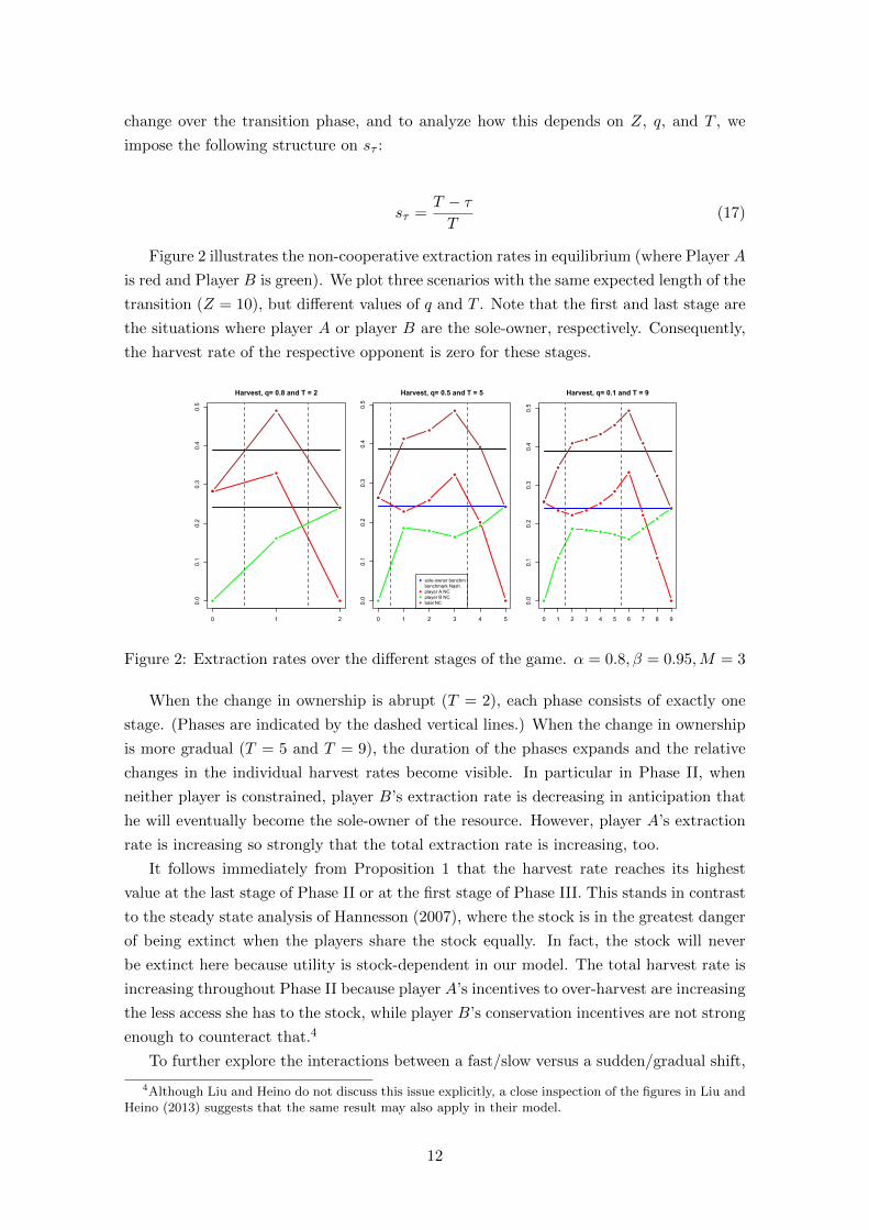
Figure 2 illustrates the non-cooperative extraction rates in equilibrium (where Player A

is red and Player B is green). We plot three scenarios with the same expected length of the

transition (Z = 10), but different values of q and T . Note that the first and last stage are

the situations where player A or player B are the sole-owner, respectively. Consequently,

the harvest rate of the respective opponent is zero for these stages.

0.0

0.1

0.2

0.3

0.4

0.5

Harvest, q= 0.8 and T = 2

0 1 2

0.0

0.1

0.2

0.3

0.4

0.5

Harvest, q= 0.5 and T = 5

0 1 2 3 4 5

sole-owner benchmbenchmark Nashplayer A NCplayer B NCtotal NC 0.

00.1

0.2

0.3

0.4

0.5

Harvest, q= 0.1 and T = 9

0 1 2 3 4 5 6 7 8 9

Figure 2: Extraction rates over the different stages of the game. α = 0.8, β = 0.95,M = 3

When the change in ownership is abrupt (T = 2), each phase consists of exactly one

stage. (Phases are indicated by the dashed vertical lines.) When the change in ownership

is more gradual (T = 5 and T = 9), the duration of the phases expands and the relative

changes in the individual harvest rates become visible. In particular in Phase II, when

neither player is constrained, player B’s extraction rate is decreasing in anticipation that

he will eventually become the sole-owner of the resource. However, player A’s extraction

rate is increasing so strongly that the total extraction rate is increasing, too.

It follows immediately from Proposition 1 that the harvest rate reaches its highest

value at the last stage of Phase II or at the first stage of Phase III. This stands in contrast

to the steady state analysis of Hannesson (2007), where the stock is in the greatest danger

of being extinct when the players share the stock equally. In fact, the stock will never

be extinct here because utility is stock-dependent in our model. The total harvest rate is

increasing throughout Phase II because player A’s incentives to over-harvest are increasing

the less access she has to the stock, while player B’s conservation incentives are not strong

enough to counteract that.4

To further explore the interactions between a fast/slow versus a sudden/gradual shift,

4Although Liu and Heino do not discuss this issue explicitly, a close inspection of the figures in Liu andHeino (2013) suggests that the same result may also apply in their model.

12

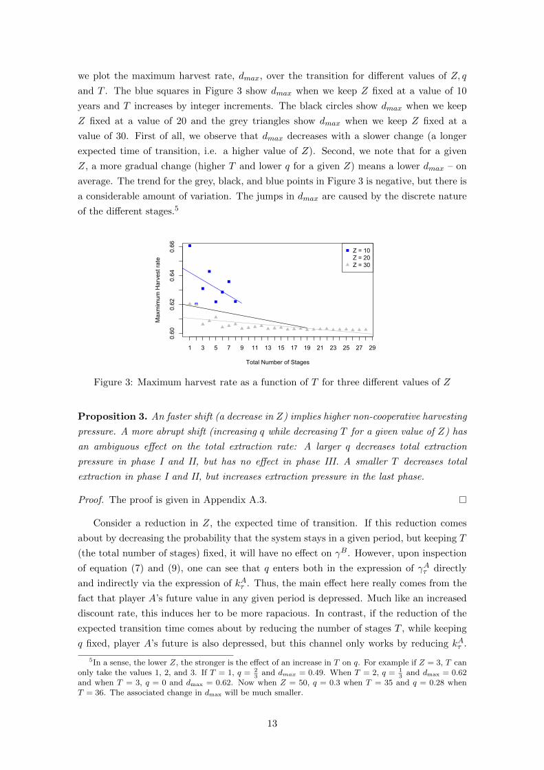
we plot the maximum harvest rate, dmax, over the transition for different values of Z, q

and T . The blue squares in Figure 3 show dmax when we keep Z fixed at a value of 10

years and T increases by integer increments. The black circles show dmax when we keep

Z fixed at a value of 20 and the grey triangles show dmax when we keep Z fixed at a

value of 30. First of all, we observe that dmax decreases with a slower change (a longer

expected time of transition, i.e. a higher value of Z). Second, we note that for a given

Z, a more gradual change (higher T and lower q for a given Z) means a lower dmax – on

average. The trend for the grey, black, and blue points in Figure 3 is negative, but there is

a considerable amount of variation. The jumps in dmax are caused by the discrete nature

of the different stages.5

0.60

0.62

0.64

0.66

Total Number of Stages

Max

mim

um H

arve

st ra

te

1 3 5 7 9 11 13 15 17 19 21 23 25 27 29

Z = 10Z = 20Z = 30

Figure 3: Maximum harvest rate as a function of T for three different values of Z

Proposition 3. An faster shift (a decrease in Z) implies higher non-cooperative harvesting

pressure. A more abrupt shift (increasing q while decreasing T for a given value of Z) has

an ambiguous effect on the total extraction rate: A larger q decreases total extraction

pressure in phase I and II, but has no effect in phase III. A smaller T decreases total

extraction in phase I and II, but increases extraction pressure in the last phase.

Proof. The proof is given in Appendix A.3.

Consider a reduction in Z, the expected time of transition. If this reduction comes

about by decreasing the probability that the system stays in a given period, but keeping T

(the total number of stages) fixed, it will have no effect on γB. However, upon inspection

of equation (7) and (9), one can see that q enters both in the expression of γAτ directly

and indirectly via the expression of kAτ . Thus, the main effect here really comes from the

fact that player A’s future value in any given period is depressed. Much like an increased

discount rate, this induces her to be more rapacious. In contrast, if the reduction of the

expected transition time comes about by reducing the number of stages T , while keeping

q fixed, player A’s future is also depressed, but this channel only works by reducing kAτ .

5In a sense, the lower Z, the stronger is the effect of an increase in T on q. For example if Z = 3, T canonly take the values 1, 2, and 3. If T = 1, q = 2

3and dmax = 0.49. When T = 2, q = 1

3and dmax = 0.62

and when T = 3, q = 0 and dmax = 0.62. Now when Z = 50, q = 0.3 when T = 35 and q = 0.28 whenT = 36. The associated change in dmax will be much smaller.

13

In addition, however, a change in T also affects player B’s strategy: A lower T means that

the scope for player B to counteract A’s overharvesting is decreased, especially in Phase

III of the game. In that phase, player A harvests all that is accessible to him, and a lower

T means that sτ , and hence player A’s harvest, is higher.

An additional measure of particular interest is the lowest biomass that the stock will

most likely obtain over the transition from player A to player B. It is of crucial impor-

tance when there are potential non-linear effects at low abundance. (We do not explicitly

consider concepts such as Allee effects or minimum viable population sizes here, but they

could of course play a critical role in the real world.) Therefore, we analyze the size of the

expected minimum stock biomass, xmin for different values of q and T (Table 1). The calcu-

lation of the expected minimum stock biomass, xmin takes into account that the expected

length that the game stays in a given period τ will affect the expected value of the biomass

at the beginning of the next stage. We assume that the game starts at the equilibrium

value x0 = M ((1− a0)M)α

1−α . To make a concrete example, suppose x0 = 10, total first-

stage equilibrium extraction d1 = 0.4 and α = 0.8,M = 3. When q = 0.5, the expected

time that the game stays in one stage is given by 11−q = 2 years. The expected value at the

beginning of stage 2 is therefore given by: x2 = M ((1− d1) [M ((1− d1)x0)α])α = 15.1.

In contrast, when q = 0.9, the game stays, on average, 10 years in a given stage, so that

the value of x at the onset of stage 2 would be x2 = 26.9, which is a lot closer to the

equilibrium value M ((1− d1)M)α

1−α = 31.5.

Table 1: Expected minimum biomass and maximum extraction rate over the transition, qis probability of staying in stage sτ ; T is number of steps. Parameters: α = 0.6;β = 0.95.

T = 2 T = 5 T = 9

q = 0.1 - -

Z = 10 years

xmin = 31.2

dmax = 0.49

q = 0.5

Z = 4 years

xmin = 23.7

dmax = 0.62

Z = 10 years

xmin = 30.1

dmax = 0.48

Z = 18 years

xmin = 30.6

dmax = 0.43

q = 0.8

Z = 10 years

xmin = 28.8

dmax = 0.49

-

Z = 45 years

xmin = 30.9

dmax = 0.41

Table 1 confirms that the slower the change, the less pressure the stock is exposed to.

Consider the second row (where q is kept fixed and T increased): As the expected duration

of the transition increases from Z = 4 years to Z = 18 years, the maximal harvest rate

declines from 0.62 to 0.43. Similarly, the expected minimal value of the stock biomass

increases from 23.7 to 30.6. While the decline in maximal harvest rate is monotone, this is

not the case for xmin: Inspection of the third column reveals that xmin actually decreases

from a value of 31.2 to a value of 30.6 when Z increases from 10 to 18 years by keeping

14

T fixed but increasing q. This non-monotonicity is driven by the fact that at q = 0.1

the game stays in a given stage for only a year on average, so that the biomass at the

expected time of transition is heavily influenced by the initial values. In contrast, the

stock is expected to stay in a given stage much longer when q = 0.5, so that the malign

effect of non-cooperation plays out longer and essentially swamps the beneficial effect of

a slower change.

Similarly, as discussed in Proposition 3 above, Table 1 shows how the effect of a

more gradual or more sudden change is not monotonic. Consider the diagonal where

Z = 10 years for all entries. As we move from the bottom-left to the top-right, the change

becomes much more gradual. However, the maximal harvest rate first decreases and then

increases. In this case, the minimal biomass actually increases steadily as the change

becomes smoother.

Finally, we consider the effect of a change in the resource’s renewability, α, and in the

discount rate β. Note that α and β always enter multiplicative as αβ in kiτ and γiτ . Hence,

in much of the literature, αβ is treated as one parameter, the “bionomic discount factor”.

Proposition 4. An increase in the bioeconomic parameters α and β leads to a lower total

extraction rate in all phases.

Proof. The proof is given in Appendix A.4.

An increase in α means the natural regrowth potential of the resource becomes weaker,

inducing the players to harvest less aggressively. By comparing (10)-(12) it becomes clear,

that this effect is strongest in the third phase, when player A’s harvesting is already

constrained by the available share of the resource, and weakest in the second phase when

neither player’s harvesting is constrained.

An increase in the discount factor, β, means that the players place a higher value on

the future harvesting opportunities. Therefore, a higher discount factor naturally leads to

a decreased extraction rate. Again, this effect is weakest in the second phase.

5 Gains from cooperation

When illustrating under which circumstances a cooperative solution could be sustained by

a self-enforcing agreement (Figure 1), we only considered whether there was any stage in

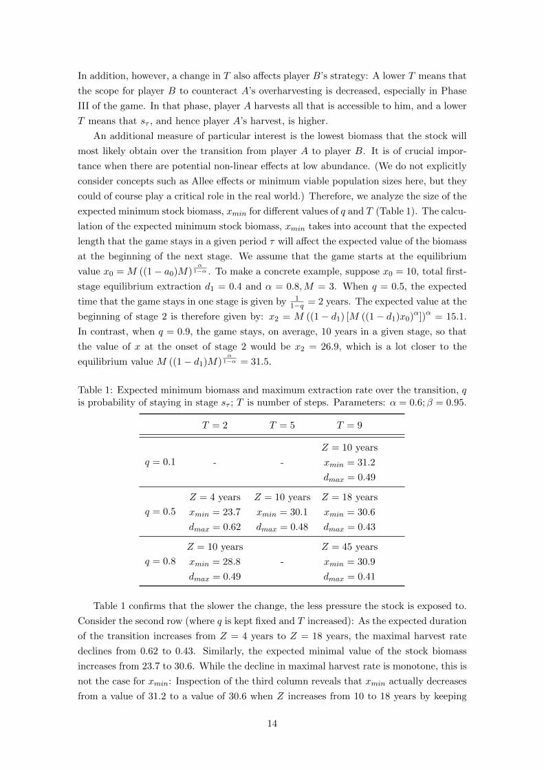
which there would be no scope for collaboration. To obtain a better insight into how the

dynamics unfold over the course of the transition, we show how the bargaining set changes

over the different stages of the game in Figure 4. In particular, it becomes obvious how

the scope for collaboration is compressed at the end and the beginning of the transition

phase. This is not surprising, as it is here that both players have the strongest bargaining

positions. Towards the end, for example, player A has nothing left to lose, but also player

B has little incentive to give him much as player A’s harvest share is constrained anyway.

Furthermore, Figure 4 illustrates how player A’s bargaining strength is declining over the

different stages, though not in a monotonic fashion. Indeed, the changes from one stage

to the next can be quite large, especially in the beginning or the end.

15

0.3

0.4

0.5

0.6

0.7

T=9, q=0.1

Sha

re la

mbd

a

1 2 3 4 5 6 7 8

0.3

0.4

0.5

0.6

0.7

T=9, q=0.5

Sha

re la

mbd

a

1 2 3 4 5 6 7 8

0.3

0.4

0.5

0.6

0.7

T=9, q=0.8

Sha

re la

mbd

a

1 2 3 4 5 6 7 8

Figure 4: Illustration of bargaining set at different stages, α = 0.6, β = 0.95

In order to speak about the potential gains from cooperation, we need to define the

social optimum. We take the stance that the first-best is achieved when the sum of

player’s utility is maximized. Note that this implies that the shift of the fish stock is in

fact immaterial. No matter who has access to what fraction of the stock, it will always

be optimal to maximize the return the resource. That is, one can disregard the transition

dynamics and simply write the social planner’s problem as choosing an extraction pattern

d and then splitting it in some arbitrary way. For simplicity, we presume that the social

planner does not discriminate between player A and player B, so that a∗ = 12d∗ and

b∗ = 12d∗. Thus, we can formulate the problem as finding the first-best total harvest as:

V ∗(x) = maxd≤1{2 ln dx+ βV ∗ (M((1− d)x)α)} (18)

As usual we can use the ‘guess and verify’ method to solve for the value function. This

confirms that V ∗ = k∗ lnx+K∗, where:

k∗ =1

1− αβ; K∗ =

1

1− β

[αβ lnαβ

1− αβ+ ln(1− αβ) +

β lnM

1− αβ− ln 2

](19)

Consequently, the first-best total extraction and the optimal steady state resource stock

are given by:

d∗ = (1− αβ); x∗ = M (αβM)α

1−α (20)

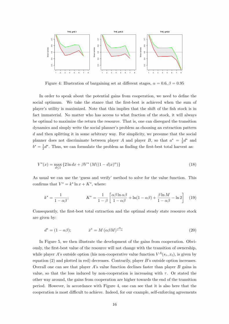
In Figure 5, we then illustrate the development of the gains from cooperation. Obvi-

ously, the first-best value of the resource will not change with the transition of ownership,

while player A’s outside option (his non-cooperative value function V A(sτ , xt), is given by

equation (2) and plotted in red) decreases. Contrarily, player B’s outside option increases.

Overall one can see that player A’s value function declines faster than player B gains in

value, so that the loss induced by non-cooperation is increasing with τ . Or stated the

other way around, the gains from cooperation are higher towards the end of the transition

period. However, in accordance with Figure 4, one can see that it is also here that the

cooperation is most difficult to achieve. Indeed, for our example, self-enforcing agreements

16

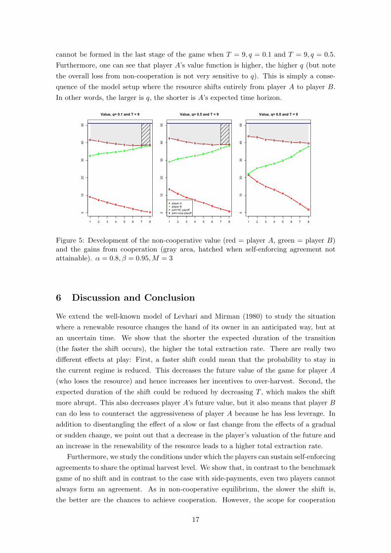
cannot be formed in the last stage of the game when T = 9, q = 0.1 and T = 9, q = 0.5.

Furthermore, one can see that player A’s value function is higher, the higher q (but note

the overall loss from non-cooperation is not very sensitive to q). This is simply a conse-

quence of the model setup where the resource shifts entirely from player A to player B.

In other words, the larger is q, the shorter is A’s expected time horizon.

010

2030

4050

Value, q= 0.1 and T = 9

1 2 3 4 5 6 7 8

010

2030

4050

Value, q= 0.5 and T = 9

1 2 3 4 5 6 7 8

player Aplayer Bjoint NC payoffjoint coop payoff 0

1020

3040

50

Value, q= 0.8 and T = 9

1 2 3 4 5 6 7 8

Figure 5: Development of the non-cooperative value (red = player A, green = player B)and the gains from cooperation (gray area, hatched when self-enforcing agreement notattainable). α = 0.8, β = 0.95,M = 3

6 Discussion and Conclusion

We extend the well-known model of Levhari and Mirman (1980) to study the situation

where a renewable resource changes the hand of its owner in an anticipated way, but at

an uncertain time. We show that the shorter the expected duration of the transition

(the faster the shift occurs), the higher the total extraction rate. There are really two

different effects at play: First, a faster shift could mean that the probability to stay in

the current regime is reduced. This decreases the future value of the game for player A

(who loses the resource) and hence increases her incentives to over-harvest. Second, the

expected duration of the shift could be reduced by decreasing T , which makes the shift

more abrupt. This also decreases player A’s future value, but it also means that player B

can do less to counteract the aggressiveness of player A because he has less leverage. In

addition to disentangling the effect of a slow or fast change from the effects of a gradual

or sudden change, we point out that a decrease in the player’s valuation of the future and

an increase in the renewability of the resource leads to a higher total extraction rate.

Furthermore, we study the conditions under which the players can sustain self-enforcing

agreements to share the optimal harvest level. We show that, in contrast to the benchmark

game of no shift and in contrast to the case with side-payments, even two players cannot

always form an agreement. As in non-cooperative equilibrium, the slower the shift is,

the better are the chances to achieve cooperation. However, the scope for cooperation

17

decreases as the change is more gradual. The scope for cooperation vanishes when the

regrowth potential of the resource is low simultaneously with a high discount factor.

Although our analytic model is fairly general, there are of course a number of (implicit)

simplifying assumptions that warrant discussion: First, we have assumed the regime shift

to be irreversible. Though clearly a simplifying assumption, it is not entirely clear what

additional insights the alternative assumption would yield. Certainly, the nature of the

game would change if the stock shifted back to the original owner at some point. Then

the player losing the stock would have more conservation incentives as it has the chance to

continue harvesting in the future. On the other hand, the player receiving the stock would

also take this into consideration and not harvest as a sole-owner, as there is a probability

to lose the stock to the original owner. This implies that the asymmetric game of the

stock shifting from one to the other player is embedded in a larger symmetric game. In

the extreme case, this larger symmetric game would converge to the benchmark game

without a shift in stock distribution.

Second, we have concentrated on the case with two players only. In general, the

literature shows the difficulty to sustain a cooperation between multiple players, especially

when no additional enforcement mechanism are available to alleviate the problem. Breton

and Keoula (2014) showed that an assumption of asymmetric players is not sufficient to

facilitate a coalition of several players, and the largest coalition size in their model is

two. In our case, the cooperation is not always possible even with two players, and if we

added a third (or several) players into the game, the possibility to achieve an agreement

may vanish entirely. However, in a recent contribution Miller and Nkuiya (2014) show

that coalition can be larger under threat of regime shift. In essence we have modeled the

transition in stock distribution as a series of exogenous regime shifts. Hence it would be

a very interesting avenue for future research to explore how the game changes when we

allow for more than two players. It goes without saying that this would require many

more structural assumptions on how the changes in the resource distribution affect the

share of the stock that the players have access to.

Finally, we have assumed that both the harvest of the players and the resource stock is

perfectly observable and common knowledge. Uncertainty about the resource stock has no

effect on the non-cooperative extraction decisions in the Levhari-Mirman game, as shown

by Antoniadou et al. (2013). When the level of individual extraction is unobservable to

society, a moral hazard problem arises, as it becomes impossible to identify the cheater and

thus target the punishment correctly. Therefore, Tarui et al. (2008) suggests a symmetric

punishment for all agents. They introduce a two-phase punishment scheme, in which a

subgame perfect equilibrium with the lowest possible payoffs is brought into play in the

first phase followed by a second phase with a forgiveness from all agents and furthermore a

stock re-establishment to the cooperative level. In line with our results, Tarui et al. (2008)

point out that a small number of players, fast growth rate of the resource or high discount

factors may not support cooperation when actions are unobservable. An alternative to

symmetric punishment could be the random punishment introduced scheme by Jensen

and Kronbak (2009), or the scheme suggested by Laukkanen (2003), according to which

18

cooperation is enforced by the threat of a sufficiently detrimental non-cooperative Nash

equilibrium. This scheme provides cooperation, but under a narrower set of conditions

than the one suggested in Tarui et al. (2008). In short, these studies indicate that including

uncertainty about the other player’s harvest (in combination with the risk-aversion implied

by a concave utility function) should lead to wider range under which cooperation is

sustainable, possibly even when there are more than two players. Whether this conjecture

indeed holds is an interesting avenue for further research.

Our model speaks to the recent difficulties that existing international fisheries agree-

ments have encountered as fish stocks have changed their spatial distribution. These

difficulties are indeed expected to increase due to climate change. A clear policy recom-

mendation that follows from our analysis is to focus attention on those cases where the

changes are expected to occur fast and smoothly. In particular, mechanisms to enlarge

the bargaining space of international fisheries by stock-unrelated side-payments should be

investigated for those cases.

19

ReferencesAcemoglu, D. (2003). Why not a political Coase theorem? Social conflict, commitment, and politics. Journal of

Comparative Economics, 31(4):620–652.

Antoniadou, E., Koulovatianos, C., and Mirman, L. J. (2013). Strategic exploitation of a common-property resourceunder uncertainty. Journal of Environmental Economics and Management, 65(1):28–39.

Barrett, S. (1994). Self-enforcing international environmental agreements. Oxford Economic Papers, 46(0):878–94.

Blenckner, T., Llope, M., Mollmann, C., Voss, R., Quaas, M. F., Casini, M., Lindegren, M., Folke, C., andChr. Stenseth, N. (2015). Climate and fishing steer ecosystem regeneration to uncertain economic futures.Proceedings of the Royal Society of London B: Biological Sciences, 282(1803).

Breton, M. and Keoula, M. Y. (2012). Farsightedness in a coalitional great fish war. Environmental and ResourceEconomics, 51(2):297–315.

Breton, M. and Keoula, M. Y. (2014). A great fish war model with asymmetric players. Ecological Economics,97:209–223.

Casini, M., Blenckner, T., Mollmann, C., Gardmark, A., Lindegren, M., Llope, M., Kornilovs, G., Plikshs, M., andStenseth, N. C. (2012). Predator transitory spillover induces trophic cascades in ecological sinks. Proceedings ofthe National Academy of Sciences, 109(21):8185–8189.

Costello, C. and Kaffine, D. (2011). Unitization of spatially connected renewable resources. The B.E. Journal ofEconomic Analysis and Policy, 11(1):1–29.

Dixit, A., Grossman, G., and Gul, F. (2000). The dynamics of political compromise. Journal of Political Economy,108(3):531–568.

Ellefsen, H. (2013). The stability of fishing agreements with entry: The northeast atlantic mackerel. StrategicBehavior and the Environment, 3(1–2):67–95.

Fesselmeyer, E. and Santugini, M. (2013). Strategic exploitation of a common resource under environmental risk.Journal of Economic Dynamics and Control, 37(1):125–136.

Hannesson, R. (2007). Global warming and fish migration. Natural Resource Modeling, 20(2):301–319.

Hannesson, R. (2013). Sharing a migrating fish stock. Marine Resource Economics, 28(1):1–17.

Harstad, B. (2013). The market for conservation and other hostages. CESifo Working Paper Series 4296, CESifoGroup Munich.

Jensen, F. and Kronbak, L. G. (2009). Random penalties and renewable resources: a mechanism to reach optimallandings in fisheries. Natural Resource Modeling, 22(3):393–414.

Kwon, O. S. (2006). Partial international coordination in the great fish war. Environmental and Resource Economics,33(4):463–483.

Laukkanen, M. (2003). Cooperative and non-cooperative harvesting in a stochastic sequential fishery. Journal ofEnvironmental Economics and Management, 45(2, Supplement):454 – 473.

Levhari, D. and Mirman, L. J. (1980). The Great Fish War: An Example Using a Dynamic Cournot-Nash Solution.The Bell Journal of Economics, 11(1):322–334.

Liu, X. and Heino, M. (2013). Comparing proactive and reactive management: Managing a transboundary fishstock under changing environment. Natural Resource Modeling, forthcoming:no–no.

Liu, X., Lindroos, M., and Sandal, L. (2012). Sharing a fish stock with density-dependent distribution and unitharvest costs. In 14th International BIOECON Conference, Cambridge, UK.

Long, N. V. (1975). Resource extraction under the uncertainty about possible nationalization. Journal of EconomicTheory, 10(1):42–53.

Long, N. V. (2010). A Survey of Dynamic Games in Economics, volume 1 of Surveys on Theories in Economicsand Business Administration. World Scientific, Singapore.

McKelvey, R., Miller, K., and Golubtsov, P. (2003). Fish wars revisited: a stochastic incomplete-information har-vesting game. In Wesseler, J., Weikard, H.-P., and Weaver, R. D., editors, Risk and Uncertainty in Environmentaland Natural Resource Economics, pages 93–112. Edward Elgar.

Miller, K. A., Munro, G. R., Sumaila, U. R., and Cheung, W. W. L. (2013). Governing marine fisheries in a changingclimate: A game-theoretic perspective. Canadian Journal of Agricultural Economics, 61(2):309–334.

Miller, S. and Nkuiya, B. (2014). Coalition formation in fisheries with potential regime shift. Unpublished WorkingPaper, University of California, Santa Barbara.

Munro, G. R. (1979). The Optimal Management of Transboundary Renewable Resources. The Canadian Journalof Economics / Revue canadienne d’Economique, 12(3):355–376.

Ryszka, K. (2013). Resource extraction in a political economy framework. Discussion Paper TI 13-094/VIII,Tinbergen Institute.

Sydsæter, K., Hammond, P., Seierstad, A., and Strøm, A. (2005). Further Mathematics for Economic Analysis.Prentice Hall, Harlow.

Tarui, N., Mason, C. F., Polasky, S., and Ellis, G. (2008). Cooperation in the commons with unobservable actions.Journal of Environmental Economics and Management, 55(1):37 – 51.

Vislie, J. (1987). On the Optimal Management of Transboundary Renewable Resources: A Comment on Munro’sPaper. The Canadian Journal of Economics / Revue canadienne d’Economique, 20(4):870–875.

20

Appendix

A.1 Proof of Proposition 1

The existence of the first phase follows from the assumption that s0 = 1 so that player A is the

sole-owner in the first stage of the game, and player B cannot extract anything. The existence

of the last phase follows from the assumption that sT = 0 and player A cannot extract anything.

The second phase may not exist (e.g. when T = 1).

Consider the first phase (equation 10). Player B’s extraction rate is constrained by the share

1− sτ accessible to him. This share is increasing as sτ is decreases. The extraction rate of player

A is given by aτ = sτγAτ . This may in principle increase or decrease. Clearly, sτ is declining with

τ , but γAτ increases with τ :

γAτ+1 − γAτ > 0 ⇔ 1

1 + αβϕAτ+1

− 1

1 + αβϕAτ> 0 ⇔ ϕAτ > ϕAτ+1

⇔ qkAτ + (1− q)kAτ+1 > qkAτ+1 + (1− q)kAτ+2

The last line is true because kAτ > kAτ+1, as we have discussed in relation to equation (7) on page

8. In spite of this indeterminacy, it is possible to show that the total extraction rate in the first

phase, which we denote dIτ for clarity, increases with τ :

dIτ+1 > dIτ ⇔ sτ+1γAτ+1 + 1− sτ+1 > sτγ

Aτ + 1− sτ

⇔ sτ+1(γAτ+1 − 1) > sτ (γAτ − 1) ⇔ sτ+1

sτ<

γAτ − 1

γAτ+1 − 1

The change in sign in the last line occurs because γAτ < 1 for all τ . The left-hand-side of the

last inequality is smaller than one as sτ+1 < sτ by construction. The right-hand side, however,

is larger than one:γAτ −1γAτ+1−1

> 1 ⇔ γAτ − 1 < γAτ+1 − 1 ⇔ γAτ+1 > γAτ . The first phase ends when

1− sτ ≥ γB(1−γAτ )1−γAτ γB

⇔ sτ ≤ αβ1−(1−αβ)γAτ

.

Consider the second phase. Equate the two non-binding best-replies aτ = γAτ (1 − bτ ) and

bτ = γB(1− aτ ) yields:

aτ = (1− γB(1− aτ ))γAτ ⇔ aτ = γAτ − γAτ γB + aτγAτ γ

B ⇔ aτ =γAτ (1− γB)

1− γAτ γB

The case for player B is symmetrical. The total extraction rate is dIIτ = aτ+bτ =γAτ (1−γB)+γB(1−γAτ )

1−γAτ γB.

It is increasing with τ when the following holds:

dIIτ+1 − dIIτ =(γAτ+1 − 2γAτ+1γ

B + γB)(1− γAτ γB)− (γAτ − 2γAτ γB + γB)(1− γAτ+1γ

B)

(1− γAτ+1γB)(1− γAτ γB)

> 0

Because the denominator is positive (γAτ < 1 and γB < 1) this is equivalent to:

(γAτ+1 − γAτ )(1 + (γB)2 − 2γB) > 0.

This inequality holds because the first bracket is positive, and since γB = 1 − αβ, the second

21

bracket reduces to (αβ)2, which is also positive.

Total extraction in the third phase is dIIIτ = sτ +(1−sτ )γB = 1−αβ+αβsτ . This is declining

as τ → T simply due to the fact that sτ > sτ+1.

A.2 Proof of Proposition 2

In the following it will be useful to define the following auxiliary parameters:

ϕAτ ≡ qkAτ + (1− q)kAτ+1 and ϕB ≡ 1

1− αβ

We start by conjecturing that V coop,iτ and V nc,iτ are of the usual log-linear form and that the

coefficients kAτ and kBτ take the form as described by equation (7). Taking the perspective of player

A, her relevant value functions are:

V coop,Aτ (λ, xt) = lnλ(1− αβ) + lnxt + ...

...β(q[kAτ lnxt+1 +Kcoop,A

τ

]+ (1− q)

[kAτ+1 lnxt+1 +KA

τ+1

])V nc,Aτ (λ, xt) = ln aτ + lnxt + ...

...β(q[kAτ lnxt+1 +Knc,A

τ

]+ (1− q)

[kAτ+1 lnxt+1 +KA

τ+1

])Note that xt+1 = M (αβxt)

αunder cooperation but xt+1 = M ((1− aτ − bτ )xt)

αunder non-

cooperation. Equating coefficients therefore shows that indeed kAτ = 1 + αβϕAτ as in the non-

cooperative case:

kAτ lnxt +Kcoop,Aτ = lnλ(1− αβ) + lnxt + ...

...β(q[kAτ (lnM + α lnαβ + α lnxt) +Kcoop,A

τ

]+ ...

... (1− q)[kAτ+1(lnM + α lnαβ + α lnxt) +KA

τ+1

])We have also:

(1− βq)Kcoop,Aτ = lnλ(1− αβ) + β

((1− q)KA

τ+1 + ϕAτ (lnM + α lnαβ))

(A-1)

For the non-cooperative case, equating coefficients yields:

(1− βq)Knc,Aτ = ln aτ + β

((1− q)KA

τ+1 + ϕAτ (lnM + α ln(1− aτ − bτ ))

(A-2)

Player A’s participation constraint is satisfied when:

V coop,Aτ (λ, xt)− V nc,Aτ (xt) = kAτ lnxt +Kcoop,Aτ −

(kAτ lnxt +Knc,A

τ

)≥ 0

Clearly, the term kAτ lnxt cancels. Similarly, inspecting (A-1) and (A-2), we see that the term

KAτ+1, capturing the further development of the game, enters in the same manner in those two

equations. Thus, it cancels as well. Therefore, we can define player A’s gain from cooperation by

gA:

22

gA(λ) =1

1− βq

(lnλ+ ln

(1− αβaτ

)+ αβϕAτ ln

(αβ

1− aτ − bτ

))(A-3)

Whether this gA(λ) > 0 is in fact independent of the current stock level and the future development

of the game.

There is not always scope for cooperation

To see that there cannot always be scope for cooperation, note that gA(λ) is increasing in λ and

reaches its maximum at λ = 1. We now show that gA(1) < 0 as αβ → 1 or q → 0, so that player

A would not join an agreement, even if she were offered the entire harvest.

To show that gA(1) < 0 as q → 0, consider A’s gain from cooperation at stage T − 1. At this

stage we have limq→0 ϕAT−1 = 0 and consequently aT−1 = sT−1 (Player A will harvest all she can

before she loses the resource for sure). We have gA(1) < 0 ⇔ ln(

1−αβaτ

)< 0 ⇔ 1 − αβ < aT−1.

When sT−1 < 1 − αβ we need to consider the game at stage τ < T − 1. But from backward

induction, it follows that aτ = sτ for all τ and consequently bτ = (1− sτ )(1−αβ). Now there will

be some τ at which sτ > 1 − αβ and since ϕAτ is bounded above by 11−αβ we know that at some

stage (as sτ → 1) we have ln(1− αβ)− (1 + αβϕAτ ) ln sτ < 0 and thus gA(1) < 0 .

Consider now the case when αβ → 1. We have that gA(1) < 0 whenever:

limαβ→1

ln

(1− αβaτ

)+ αβϕAτ ln

(αβ

1− aτ − bτ

)< 0

To evaluate this limit, we need a few building stones. Consider first kAτ , ϕAτ and γAτ , where we

use L’Hopital’s rule to show that these terms converge to some constant κ:

limαβ→1

kAτ = limαβ→1

[1

1− αβ

(1−

(αβ(1− q)1− αβq

)T−τ)]

=

limαβ→1

[−(T − τ)

(αβ(1−q)1−αβq

)T−τ−1 (1−q

(1−αβq)2

)]limαβ→1−1

= (T − τ) limαβ→1

[(αβ(1− q)1− αβq

)T−τ−1]

limαβ→1

[1− q

(1− αβq)2

]=T − τ1− q = κ1 > 0

limαβ→1

ϕAτ = limαβ→1

qkAτ + (1− q)kAτ+1 = q(T − τ)

(1− q) + T − τ − 1 = κ2 > 0

limαβ→1

γAτ = limαβ→1

1

1 + αβϕA= κ3 > 0

limαβ→1

γB = limαβ→1

(1− αβ) = 0

And therefore:

limαβ→1

aτ =

limαβ→1 sτγ

Aτ = sτκ3 Phase I

limαβ→1γAτ (1−γB)

1−γAτ γB= κ3 Phase II

limαβ→1 sτ = sτ Phase III

limαβ→1

bτ =

limαβ→1 1− sτ = 1− sτ

limαβ→1γB(1−γAτ )

1−γAτ γB= 0

limαβ→1(1− sτ )γB = 0

23

Hence, limαβ→1 ln(

1−αβaτ

)= −∞, but limαβ→1 αβϕ

Aτ ln

(αβ

1−aτ−bτ

)= κ2 ln

(1

1−sτκ3

)in Phase I,

= κ2 ln(

11−κ3

)in Phase II, and = κ2 ln

(1

1−sτ

)in Phase III. In any case, it is bounded above so

that the entire term[ln(

1−αβaτ

)+ αβϕAτ ln

(αβ

1−aτ−bτ

)]must be smaller than zero as claimed.

Derivation of λAmin and λBmax

Now consider the situation where αβ take values such that gA(λAmin) = 0 exists. By re-writing

equation (A-3) and taking exponents on both sides, we get:

λAmin =aτ

1− αβ

(1− aτ − bτ

αβ

)αβϕAτ(15)

By parallel reasoning, player B’s participation constraint is satisfied when V coop,Bτ − V nc,Bτ ≥ 0

and λBmax, the maximum share that player B would be willing to give to player A and still harvest

cooperatively is – if it exists – defined by:

λBmax = 1− bτ1− αβ

(1− aτ − bτ

αβ

)αβϕB(16)

Cooperation possibilities are not constrained by the available harvest shares

At any stage τ , player A needs to harvest at least (1−αβ)λAmin to join the agreement. This is less

than he would harvest under non-cooperation:

(1− αβ)λAmin < aτ ⇔ aτ

(1− aτ − bτ

αβ

)αβϕAτ< aτ ⇔

(1− aτ − bτ

αβ

)αβϕAτ< 1

The last statement is true because 1−aτ −bτ = 1−dnc < 1−d∗ = αβ and αβϕ > 0 and a function

xy < 1 when x < 1 and y > 0. For player B, the argumentation is parallel:

(1− αβ)(1− λBmax) < bτ ⇔ bτ

(1− aτ − bτ

αβ

)αβϕB< bτ ⇔

(1− aτ − bτ

αβ

)αβϕB< 1

As aτ ≤ sτ and bτ ≤ 1− sτ by construction, it follows immediately that cooperation possibilities

are not constrained by the accessible harvest shares.

This completes the proof of Proposition 2.

A.3 Proof of Proposition 3

To show how the extraction pattern changes with we need to derive∂γAτ∂q (kB and thus γB do not

depend on q). In this derivation, we will again employ the following auxiliary parameters to make

the derivations more concise.

ϕAτ ≡ qkAτ + (1− q)kAτ+1 and ϕB ≡ 1

1− αβ

To start, consider∂kAτ∂q :

24

∂kAτ∂q

=−(T − τ)

(αβ(1−q)1−αβq

)T−τ−1 (−αβ(1−αβq)−αβ(1−q)(−αβ)(1−αβq)2

)1− αβ

= −(T − τ)

(αβ(1− q)1− αβq

)T−τ−1( −αβ(1− αβq)2

)> 0 (A-4)

The above follows from T > τ and because the term(αβ(1−q)1−αβq

)> 0 as α, β, and q ∈ (0, 1). As a

consequence:

∂ϕAτ∂q

= kAτ + q∂kAτ∂q− kAτ+1 + (1− q)

∂kAτ+1

∂q

= kAτ − kAτ+1 + q

(∂kAτ∂q−∂kAτ+1

∂q

)+∂kAτ+1

∂q> 0 (A-5)

Here, we have to show that∂kAτ∂q >

∂kAτ+1

∂q for all kAτ > kAτ+1 and q > 0 and∂kAτ+1

∂q > 0. From (A-4)

we have:

∂kAτ∂q−∂kAτ+1

∂q> 0⇔ (T − τ − 1)

(αβ(1− q)1− αβq

)T−τ−2− (T − τ)

(αβ(1− q)1− αβq

)T−τ−1> 0

⇔ (T − τ − 1)

(1− αβqαβ(1− q)

)> T − τ

⇔ T − τ − 1 > αβ(T − τ − q)

This is true because α, β, and q ∈ (0, 1). This implies:

∂γAτ∂q

=−αβ ∂ϕ

Aτ

∂q

(1 + αβϕA)2< 0 (A-6)

Furthermore, we need to derive∂γAτ∂T (kB and thus ϕB and γB do not depend on T .). Again,

consider first∂kAτ∂T :

∂kAτ∂T

=−1

1− αβ

(αβ(1− q)1− αβq

)T−τln

(αβ(1− q)1− αβq

)> 0 (A-7)

Since(αβ(1−q)1−αβq

)< 1, the logarithm yields a negative number, so that the entire term is positive.

Consequently:

∂ϕAτ∂T

= q∂kAτ∂T

+ (1− q)∂kAτ+1

∂T> 0 (A-8)

∂γAτ∂T

=−αβ ∂ϕ

Aτ

∂T

(1 + αβϕA)2< 0 (A-9)

In the first phase, player B is harvesting the entire share available to him (bIτ = 1− sτ ). Hence

his extraction rate does not depend on q. It does depend on T , however, since sτ = T−τT . sτ

25

increases with T so that bIτ decreases. From (A-6), it follows that player A’s and thus the total

extraction rate is decreasing in q. Regarding an increase in T , we see from (A-9) that γAτ decreases,

but sτ increases. The total effect is still negative:

∂dIτ∂T

=∂sτ∂T

γAτ + sτ∂γAτ∂T− ∂sτ∂T

< 0

⇔ ∂sτ∂T

γAτ + sτ∂γAτ∂T− ∂sτ∂T

< 0

⇔ sτ∂γAτ∂T

< (1− γAτ )∂sτ∂T

This is true because∂γAτ∂T < 0 and all other terms are positive (and γAτ < 1).

In the second phase, we have dII =γAτ +γB−2γAτ γ

B

1−γAτ γB. Consequently:

∂dIIτ∂q

=

(∂γAτ∂q −

∂2γAτ γB

∂q

)(1− γAτ γB)− ∂(1−γAτ γ

B)∂q (γAτ + γB − 2γAτ γ

B)

(1− γAτ γB)2

=

(∂γAτ∂q − 2γB

∂γAτ∂q

)(1− γAτ γB) + γB

∂γAτ∂q (γAτ + γB − 2γAτ γ

B)

(1− γAτ γB)2

=(1− γB)2

∂γAτ∂q

(1− γAτ γB)2=

(αβ)2∂γAτ∂q

(1− γAτ γB)2

As we know, (αβ)2 > 0 and∂γAτ∂q < 0 (confer (A-6)), which implies a negative nominator and a

positive denominator. Consequently, the total extraction is decreasing in q.

Similarly:

∂dIIτ∂T

=

(∂γAτ∂T −

∂2γAτ γB

∂T

)(1− γAτ γB)− ∂(1−γAτ γ

B)∂T (γAτ + γB − 2γAτ γ

B)

(1− γAτ γB)2

=(αβ)2

∂γAτ∂T

(1− γAτ γB)2

Again, (αβ)2 > 0 and∂γAτ∂T < 0 (following from (A-9)) , which implies a negative nominator and a

positive denominator. Consequently, the total extraction is decreasing in T in the second phase.

In the third phase, neither player’s extraction rate reacts to changes in q. Instead, both player’s

extration rates depend on T as aIIIτ = sτ and bIIIτ = (1 − sτ )γB . As an increase in T means a

larger sτ , the extraction rate of player A increases in T , and consequently player B’s extraction

rate decreases. The total effect is increasing, as player B’s declining effect is smaller than the effect

of player A (1− αβ < 1).

A.4 Proof of Proposition 4

To see that an increase in α or β (and hence αβ) leads to a lower total extraction rate in all phases,

we first need to establish∂γAτ∂αβ < 0 and ∂γB

∂αβ < 0. As γB = 1− αβ, the sign of the latter derivative

26

is obvious. For γAτ = (1 + αβ(qkAτ + (1 − q)kAτ+1))−1, it is more involved. We first need to show

that∂kAτ∂αβ > 0:

∂kAτ∂αβ

=

(1−

(αβ(1−q)1−αβq

)T−τ)− (T − τ)

(αβ(1−q)1−αβq

)T−τ−1 ( (1−q)(1−αβq)+αβq(1−q)(1−αβq)2

)(1− αβ)

(1− αβ)2> 0

⇔(

1−(αβ(1− q)1− αβq

)T−τ)> (T − τ)

(αβ(1− q)1− αβq

)T−τ−1 ( (1− q)(1− αβ)

(1− αβq)2

)

⇔(αβ(1− q)1− αβq

)τ−T− 1 > (T − τ)

(1− αβqαβ(1− q)

)(1− q)(1− αβ)

(1− αβq)2

⇔(

1− αβqαβ − αβq

)T−τ− 1 > (T − τ)

1− αβαβ(1− αβq)

We know that this holds because at τ = T − 1 (the largest value that τ can take at which kAτ is

still strictly positive), the last line reads: 1−αβqαβ−αβq − 1 > 1−αβ

αβ(1−αβq) . This can be transformed to

q(1−αβ)2 > 0 which is true because q < 1 and αβ < 1. For τ > T − 1 the left-hand-side (LHS) of

the above inequality is growing exponentially while the right-hand-side (RHS) is growing linearly.

The subsequent comparative static results follow immediately from∂kAτ∂αβ > 0:

∂[qkAτ + (1− q)kAτ+1]

∂αβ= q

∂kAτ∂αβ

+ (1− q)∂kAτ+1

∂αβ> 0

∂γAτ∂αβ

=−[qkAτ + (1− q)kAτ+1]− αβ ∂[qk

Aτ +(1−q)kAτ+1]

∂αβ

(1 + αβ[qkAτ + (1− q)kAτ+1])2< 0 (A-10)

In the first phase, Player B’s extraction rate is given by bIτ = 1 − sτ and does not depend on

αβ. Player A’s extraction rate in the first phase is given by aIτ = sτγAτ and

∂aIτ∂αβ = sτ

∂γAτ∂αβ < 0,

which follows from (A-10).

In Phase II, total extraction is dIIτ = aIIτ + bIIτ =γAτ (1−γB)1−γAτ γB

+γB(1−γAτ )1−γAτ γB

=γAτ +γB−2γAτ γ

B

1−γAτ γB.

Consequently:

∂dIIτ∂αβ

=

(∂γAτ∂αβ + ∂γB

∂αβ −∂2γAτ γ

B

∂αβ

)(1− γAτ γB)− ∂(1−γAτ γ

B)∂αβ (γAτ + γB − 2γAτ γ

B)

(1− γAτ γB)2

=

(∂γAτ∂αβ − 1 + 2γAτ − 2γB

∂γAτ∂αβ

)(1− γAτ γB)− (γAτ − γB

∂γAτ∂αβ )(γAτ + γB − 2γAτ γ

B)

(1− γAτ γB)2

=(αβ)2

∂γAτ∂αβ − (1− γAτ )2

(1− γAτ γB)2

As (αβ)2 > 0,∂γAτ∂αβ < 0 and (1−γAτ )2 > 0, the nominator is negative. Additionally, the denominator

is (1− γAτ γB)2 > 0, and consequently the total extraction is decreasing in αβ in the second phase.

In the third phase, player A’s extraction rate is independent of α and β, and thus changes in

those do not affect her extraction rate. However, player B’s extraction is linearly dependent on

both α and β as bτ = (1− sτ )1− αβ, and an increase in those parameters results in a decrease in

player B’s, and consequently in the total extraction rate.

27

Fisheries agreements with a shifting stock Online Appendix

[This section is intended as online appendix.]

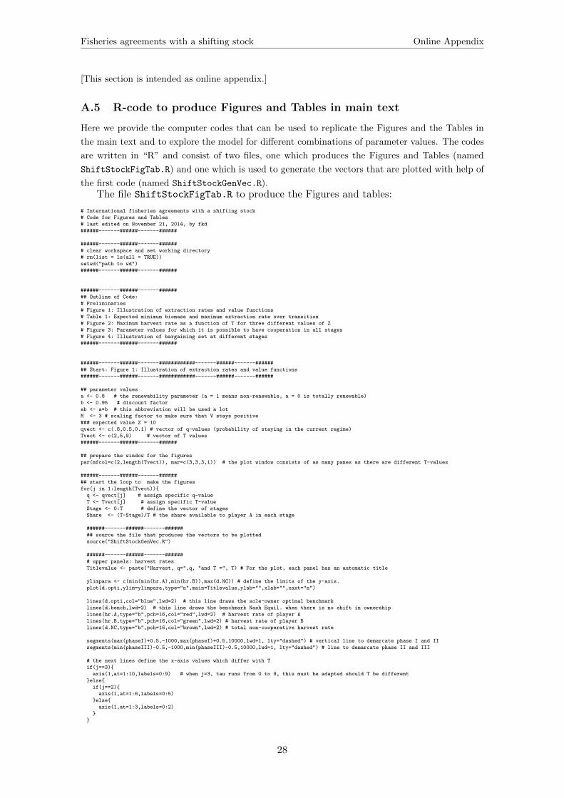
A.5 R-code to produce Figures and Tables in main text

Here we provide the computer codes that can be used to replicate the Figures and the Tables in

the main text and to explore the model for different combinations of parameter values. The codes

are written in “R” and consist of two files, one which produces the Figures and Tables (named

ShiftStockFigTab.R) and one which is used to generate the vectors that are plotted with help of

the first code (named ShiftStockGenVec.R).The file ShiftStockFigTab.R to produce the Figures and tables:

# International fisheries agreements with a shifting stock

# Code for Figures and Tables

# last edited on November 21, 2014, by fkd

######-------######-------######

######-------######-------######

# clear workspace and set working directory

# rm(list = ls(all = TRUE))

setwd("path to wd")

######-------######-------######

######-------######-------######

## Outline of Code:

# Preliminaries

# Figure 1: Illustration of extraction rates and value functions

# Table 1: Expected minimum biomass and maximum extraction rate over transition

# Figure 2: Maximum harvest rate as a function of T for three different values of Z

# Figure 3: Parameter values for which it is possible to have cooperation in all stages

# Figure 4: Illustration of bargaining set at different stages

######-------######-------######

######-------######-------############-------######-------######

## Start: Figure 1: Illustration of extraction rates and value functions

######-------######-------############-------######-------######

## parameter values

a <- 0.8 # the renewability parameter (a = 1 means non-renewable, a = 0 is totally renewable)

b <- 0.95 # discount factor

ab <- a*b # this abbreviation will be used a lot

M <- 3 # scaling factor to make sure that V stays positive

### expected value Z = 10

qvect <- c(.8,0.5,0.1) # vector of q-values (probability of staying in the current regime)

Tvect <- c(2,5,9) # vector of T values

######-------######-------######

## prepare the window for the figures

par(mfcol=c(2,length(Tvect)), mar=c(3,3,3,1)) # the plot window consists of as many panes as there are different T-values

######-------######-------######

## start the loop to make the figures

for(j in 1:length(Tvect)){

q <- qvect[j] # assign specific q-value

T <- Tvect[j] # assign specific T-value

Stage <- 0:T # define the vector of stages

Share <- (T-Stage)/T # the share available to player A in each stage

######-------######-------######

## source the file that produces the vectors to be plotted

source("ShiftStockGenVec.R")

######-------######-------######

# upper panels: harvest rates

Titlevalue <- paste("Harvest, q=",q, "and T =", T) # For the plot, each panel has an automatic title

ylimpara <- c(min(min(hr.A),min(hr.B)),max(d.NC)) # define the limits of the y-axis.

plot(d.opti,ylim=ylimpara,type="n",main=Titlevalue,ylab="",xlab="",xaxt="n")

lines(d.opti,col="blue",lwd=2) # this line draws the sole-owner optimal benchmark

lines(d.bench,lwd=2) # this line draws the benchmark Nash Equil. when there is no shift in ownership

lines(hr.A,type="b",pch=16,col="red",lwd=2) # harvest rate of player A

lines(hr.B,type="b",pch=16,col="green",lwd=2) # harvest rate of player B

lines(d.NC,type="b",pch=16,col="brown",lwd=2) # total non-cooperative harvest rate

segments(max(phaseI)+0.5,-1000,max(phaseI)+0.5,10000,lwd=1, lty="dashed") # vertical line to demarcate phase I and II

segments(min(phaseIII)-0.5,-1000,min(phaseIII)-0.5,10000,lwd=1, lty="dashed") # line to demarcate phase II and III

# the next lines define the x-axis values which differ with T

if(j==3){

axis(1,at=1:10,labels=0:9) # when j=3, tau runs from 0 to 9, this must be adapted should T be different

}else{

if(j==2){

axis(1,at=1:6,labels=0:5)

}else{

axis(1,at=1:3,labels=0:2)

}

}

28

lg.text <- c("sole-owner benchm", "benchmark Nash", "player A NC", "player B NC", "total NC") # text for legend

legend("bottomleft",lg.text, pch = 16,col=c("blue","black","red","green","brown"),cex=0.7) # place legend in plot

rm(lg.text,ylimpara) # remove the variables lg.text and ylimpara

######-------######-------######

# plots of value function

Titlevalue <- paste("Value, q=",q, "and T =", T)

plot(V.A.expect, type="b",col="red",lwd=2,ylim=c(0,V.SO.expect),main=Titlevalue,ylab="",xlab="",xaxt="n") # value function of player A

lines(V.B.expect,type="b",col="green",lwd=2) # value function of player B

segments(-1,V.SO.expect,T+10,V.SO.expect,col="blue",lwd=2) # indicating Sole-owner payouts

segments(max(phaseI)+0.5,-1000,max(phaseI)+0.5,10000,lwd=1, lty="dashed") # vertical line to demarcate phase I and II

segments(min(phaseIII)-0.5,-1000,min(phaseIII)-0.5,10000,lwd=1, lty="dashed") # line to demarcate phase II and III

if(j==3){

axis(1,at=1:10,labels=0:9)

}else{

if(j==2){

axis(1,at=1:6,labels=0:5)

}else{

axis(1,at=1:3,labels=0:2)

}

}

lg.text <- c("player A", "player B", "sole-owner benchm") # yes, correct

legend("topleft",lg.text, pch = 16,col=c("red","green","blue"),cex=0.7)

}

######-------######-------############-------######-------######

## End: Figure 1

######-------######-------############-------######-------######

######-------######-------############-------######-------######

## Start: Table 1: Expected minimum biomass and maximum extraction rate over transition

######-------######-------############-------######-------######

## parameter values

a <- 0.8 # the renewability parameter (a = 1 means non-renewable, a = 0 is totally renewable)

b <- 0.95 # discount factor

ab <- a*b # this abbreviation will be used a lot

M <- 3 # scaling factor to make sure that V stays positive

qvect <- c(.1,0.5,0.8) # the different values of q to be tabulated

Tvect <- c(2,5,9) # the different values of T to be tabulated

######-------######-------######

## create empty tables to be filled with values

XminTable <- matrix(NA,length(qvect),length(Tvect))

dmaxTable <- matrix(NA,length(qvect),length(Tvect))

## loop through q- and T-values to fill table

for(i in 1:length(qvect)){ #i-loop through q (rows in Table 1)

for(j in 1:length(Tvect)){ #j-loop through T (columns in Table 1)

q <- qvect[i]

T <- Tvect[j]

Stage <- 0:T

Share <- (T-Stage)/T

source("ShiftStockGenVec.R") # obtain vector of total harvest rates and x-values

XminTable[i,j] <- round(min(xdev[,expttime]),1) # minimum expected biomass for a given scenario

dmaxTable[i,j] <- round(max(d.NC),2) # maximum harvest rate for a given scenario

}}

######-------######-------############-------######-------######

## End: Table 1

######-------######-------############-------######-------######

######-------######-------############-------######-------######

## Start: Figure 2: Maximum harvest rate as a function of T for three different values of Z

######-------######-------############-------######-------######

## parameter values

a <- 0.8 # the renewability parameter (a = 1 means non-renewable, a = 0 is totally renewable)

b <- 0.95 # discount factor

ab <- a*b # this abbreviation will be used a lot

M <- 3 # scaling factor to make sure that V stays positive

Zvect <- c(10,20,30) # vector of expected transition times to evaluate

######-------######-------######

## create the vectors for plotting

for(j in 1:3){ # j-loop through the different Z values

Z <- Zvect[j]

Tvect <- 1:(Z-1) # for a given Z, return the possible integer values of T

dmaxPlot <- rep(NA,length(Tvect)) # create an empty vector to later store the values if max hatrvest rate dmax

for(i in 1:length(Tvect)){ # i-loop through the different values of T (total number of stages)

T <- Tvect[i]

q <- 1-(T/Z) # find the value of q that corresponds to given Z and T

Stage <- 0:T

Share <- (T-Stage)/T

source("ShiftStockGenVec.R") # source the file that creates the vector of total harvest rates

dmaxPlot[i] <- max(d.NC) # find the maximum harvest rate for a given combination of q,T, and Z

if(j==1){

dmaxPlot.10 <- dmaxPlot # maximum harvest rate when Z = 10

29

}else{

if(j==2){

dmaxPlot.20 <- dmaxPlot # maximum harvest rate when Z = 20

}else{

dmaxPlot.30 <- dmaxPlot # maximum harvest rate when Z = 30

}}}}

######-------######-------######

## plot the vectors of maximum harvest rates

# reset the window for plotting

par(mfcol=c(1,1), mar=c(5,4,4,2)) #margins=c(bottom, left, top, right)

plot(dmaxPlot,ylim=c(0.4,0.5),

type="n",ylab="Maxmimum Harvest rate",xlab="Total Number of Stages",xaxt="n")

points(dmaxPlot.10,col="blue",pch=15)

points(dmaxPlot.20,col="black",pch=16)

points(dmaxPlot.30,col="gray",pch=17)

axis(1,at=1:30,labels=0:29)

lg.text <- c("Z = 10", "Z = 20", "Z = 30") # yes, correct

legend("topright",lg.text, pch = c(15,16,17),col=c("blue","black","gray"))

######-------######-------############-------######-------######

## End: Figure 2

######-------######-------############-------######-------######

######-------######-------############-------######-------######

## Start: Figure 3: Parameter values for which it is possible to have cooperation in all stages

######-------######-------############-------######-------######

## parameter values

abvect <- seq(0.5,0.9,length=10) # the vectors of alpha*beta to be investigated

qvect <- seq(0.5,0.9,length=20) # the vector of q

Tvect <- c(5,10,15) # three different values of T that will be plotted

M <- 3 # scaling factor to make sure that V stays positive

## create empty table to be filled with values of 0 if no cooperation and 1 if cooperation

Mat <- matrix(NA,length(abvect),length(qvect))

######-------######-------######

## start the loop: for each T fill Mat, this takes a long time depending on length of ab- and q-vector

for(Tcounter in 1:3){

T <- Tvect[Tcounter] #

Stage <- 0:T

Share <- (T-Stage)/T

for(i in 1:length(abvect)){

for(j in 1:length(qvect)){

ab <- abvect[i]

a <- sqrt(ab) # the source code needs alpha and beta separately, so simply split ab evenly

b <- sqrt(ab)

q <- qvect[j]

source("ShiftStockGenVec.R")

laA.min <- (hr.A/d.opti)*((1-d.NC)/(1-d.opti))^(ab*varphi.A) # lambda min according to eq(24) in main text

laB.max <- 1-(hr.B/d.opti)*((1-d.NC)/(1-d.opti))^(ab*varphi.B) # lambda max according to eq(25) in main text

Gamma <- laB.max-laA.min # scope for cooperation?

Gamma <- Gamma[2:T] # do not look at first stage when player A is sole-owner

if(min(Gamma)>=0){Mat[i,j] <- 1}else{Mat[i,j] <- 0}

}

}

## store the scope-for-cooperation matrix of the different T-scenarios

if(Tcounter==1){MatT5 <- Mat}else{

if(Tcounter==2){MatT10 <- Mat}else{MatT15 <- Mat}

}}

## preparations for the plot

library(lattice) # load the package to do the contourplots

col.regions <- c("red", "blue", "green") # give gridcell a green colour when coop possible in all stages, red if not

## plotting the tables

contourplot(MatT5,cuts=2,col.regions=col.regions,colorkey=FALSE,contour=F,region=T,

xlab="alpha*beta between 0.5 and 0.9",ylab="q between 0.5 and 0.9",

main="T = 5")

contourplot(MatT10,cuts=2,col.regions=col.regions,colorkey=FALSE,contour=F,region=T,

xlab="alpha*beta between 0.5 and 0.9",ylab="q between 0.5 and 0.9",

main="T = 10")

contourplot(MatT15,cuts=2,col.regions=col.regions,colorkey=FALSE,contour=F,region=T,

xlab="alpha*beta between 0.5 and 0.9",ylab="q between 0.5 and 0.9",

main="T = 15")

######-------######-------############-------######-------######

## End: Figure 3

######-------######-------############-------######-------######

######-------######-------############-------######-------######

## Start: Figure 4: Illustration of bargaining set at different stages

######-------######-------############-------######-------######

## parameter values

a <- 0.6 # the renewability parameter (a = 1 means non-renewable, a = 0 is totally renewable)

b <- 0.95 # discount factor

ab <- a*b # this abbreviation will be used a lot

M <- 3 # scaling factor to make sure that V stays positive

T <- 9 # holding total number of stages fixed

Stage <- 0:T

Share <- (T-Stage)/T

qvect <- c(0.1,0.5,0.8) # evaluating three different values of q

30

######-------######-------######

## plot bargaining set over different stages

# prepare window for plotting

par(mfcol=c(1,length(qvect)), mar=c(3,4,4,2)) #margins=c(bottom, left, top, right)

for(i in 1:length(qvect)){ # i-loop through different values of q

q <- qvect[i]

source("ShiftStockGenVec.R")

laB.max <- 1-(hr.B/d.opti)*((1-d.NC)/(1-d.opti))^(ab*varphi.B) # vector of maximal share that B is willing to give at stage tau

laA.min <- (hr.A/d.opti)*((1-d.NC)/(1-d.opti))^(ab*varphi.A) # minimal share that A needs to receive at stage tau

cooptime <- which(laB.max-laA.min>0) # find the stages at which cooperation is at all possible

Titlevalue <- paste("T =9, q=",q) # For the plot, each panel has an automatic title

# create the empty plot

plot(2:T,2:T,ylim=c(0.25,0.75),type="n",ylab="Share lambda",xlab="Stage tau",main=Titlevalue,xaxt="n")

# fill the bargaining set at which cooperation is possible

polygon(c(cooptime,rev(cooptime),min(cooptime)),c(laA.min[cooptime],rev(laB.max[cooptime]),laA.min[min(cooptime)]),col=gray(0.92),border=gray(1))

lines(cooptime,laA.min[cooptime],lwd=2) # this (lower) line gives the minimal share that A needs to receive

lines(cooptime,laB.max[cooptime],lwd=2) # this (upper) line gives the maximal share that B is willing to give

segments(-1,0.5,T+2,0.5,lty="dotted") # dotted line to indicate a 50/50 split

axis(1,at=2:T,labels=1:8)

}

######-------######-------############-------######-------######

## End: Figure 4

######-------######-------############-------######-------######

The file ShiftStockGenVec.R that generates the vectors to be plotted:

## code to generate vectors and values for plotting, used in ShiftStockFigTab

# last edited on June 22, 2015, by fkd

######-------######-------######

######-------######-------######

# needs input a, b, ab, q, T, Stage, and Share

# produces output: d.NC,d.opti,d.bench,,hr.A,hr.B,

# xdev,exptime,varphi.A,varphi.B,phaseI,phaseIII

# V.SO.expect,V.A.expect,V.B.expect

######-------######-------######

######-------######-------######

## construct the derived parameters, k.tau, varphi.A, gamma

k.B <- 1/(1-ab) # initial values

kTA <- 0 # initial values

k.A <- c(rep(NA,T),kTA) # k for player A (0 to make space for them first)

varphi.A <- c(rep(NA,T),0) # varphi for player A (0 to make space for them first)

gamma.A <- c(rep(NA,T),0) # gamma for player A (0 to make space for them first)

for(t in T:0){

k.A[t] <- (1+ab*(1-q)*k.A[t+1])/(1-ab*q) # according to equation 11

}

for(t in T:0){

varphi.A[t] <- (q*k.A[t] + (1-q)*k.A[t+1])

}

varphi.B <- rep(1/(1-ab),length(varphi.A))

for(t in T:0){

gamma.A[t] <- 1/(1+ab*(q*k.A[t] + (1-q)*k.A[t+1])) # according to eq 13

}

gamma.B <- rep((1-ab),length(gamma.A)) # according to eq 14

######-------######-------######

######---------------------------------------------#######

## PART 1. Harvesting rates

######---------------------------------------------#######

######-------######-------######

## harvesting rates

## benchmarks

d.opti <- rep((1-ab),length(Stage)) # optimal harvesting rate

d.bench <- rep(2*(1-ab)/(2-ab),length(Stage)) # benchmark NC game harv rate

## theoretical (unconstrained harvest rates; eq 9)

hr.A <- (gamma.A*(1-gamma.B))/(1-gamma.A*gamma.B)

hr.B <- (gamma.B*(1-gamma.A))/(1-gamma.A*gamma.B)

## for info: where does Phase I, II, and, III begin and end?

(phaseI <- which(hr.B>=(1-Share)))

(phaseIII <- which(hr.A>=Share))

hr.A[phaseI] <- Share[phaseI]*gamma.A[phaseI]

hr.B[phaseI] <- 1-Share[phaseI]

hr.A[phaseIII] <- Share[phaseIII]

hr.B[phaseIII] <- (1-Share[phaseIII])*gamma.B[phaseIII]

d.NC <- hr.A + hr.B

31

# remove those variables that are no longer needed:

rm(gamma.A,gamma.B,t)

######---------------------------------------------#######

## PART 2. Optimal Value and Non-cooperative value

######---------------------------------------------#######

## scale M so that biomass always above 1...

Mnecessary <- (1-max(d.NC))^(-a)*(Share[T])^(a-1) # to check whether M from input is really large enough so that V is always positive

M <- max(M,Mnecessary)

rm(Mnecessary)

######-------######-------######

# calculate the biomass values:

x.opti <- M*((1-d.opti)*M)^(a/(1-a)) # first-best

x.bench <- M*((ab/(2-ab))*M)^(a/(1-a)) # benchmark Nash equilibrium if there is no shift in ownership

# biomass when game stays long enough in each stage to reach equilibrium

x.equil.NC <- M*((1-d.NC)*M)^(a/(1-a))

# biomass when game stays the expected time in each stage

# to find these values create matrix in which stock development is calculated

# and then pick the value of x which corresponds to the expected time the game stays in each stage

expttime <- round(1/(1-q)) # what is the expected time that the game stays in each stage?

if(expttime==0){expttime <- 1} # as robustness when q very low exptime could be zero, avoid that

maxlength <- 100 # upper bound for periods to be calculated

xdev <- matrix(NA,T,maxlength) # empty matrix top be filled with values

xconvcheck <- x.equil.NC[1:T] # vector of equilibrium values to check whether procedure converges/how far exttime is from equilbrium

xdev[1,1] <- x.equil.NC[1] # initial value is equilibrium in stage zero

for(l in 1:T){ # l-loop through all stages

if(l>1){xdev[l,1] <- xdev[l-1,expttime+1]} # the initial value at stage tau+1 is the updated last value from stage tau

for(k in 2:(maxlength)){

xdev[l,k] <- M*(xdev[l,k-1]*(1-d.NC[l+1]))^a # calculate stock development according to equation 1 in main text

}

}

x.expect.NC <- c(x.equil.NC[1],xdev[,expttime+1])

# xdev[,c(1,round(maxlength/2),maxlength)] # to check convergence

rm(maxlength,xconvcheck,l)

######-------######-------######

######-------######-------######

## benchmark NC values

k.star <- 1/(1-ab)

## Sole-owner benchmark

K.SO <- (log(1-ab)+(ab*log(ab)+b*log(M))/(1-ab))/(1-b)

V.SO <- k.star*log(x.opti[1])+K.SO # assuming that x has reached SO equil level

V.SO.expect <- k.star*log(x.expect.NC[T+1])+K.SO # assuming that x is at expected level of last transition

## Social Optimum

K.FirstBest <- (log(1-ab)+(ab*log(ab)+b*log(M))/(1-ab)-log(2))/(1-b)

FirstBest <- 2*(k.star*log(x.opti[1])+K.FirstBest)

## bench

K.benchNC <- (log(1-ab)+(ab*log(ab)+b*log(M))/(1-ab) - ((2-ab)/(1-ab))*log(2-ab))/(1-b)

V.benchNC <- k.star*log(x.bench)+K.benchNC

######-------######-------######

######-------######-------######

# derived values of K_tau

K.A <- c(rep(NA,T),kTA)

K.B <- c(rep(NA,T),K.SO)

for(t in T:0){

K.A[t] <- (((1-b*q)^(-1))*

(log(hr.A[t]) + b*((q*k.A[t]+(1-q)*k.A[t+1])*(a*log(1-d.NC[t])+log(M))) + b*(1-q)*K.A[t+1]))

K.B[t] <- ((1/(1-b*q))*

(log(hr.B[t]) + (b/(1-ab))*(a*log(1-d.NC[t])+log(M)) + b*(1-q)*K.B[t+1]))

}

######-------######-------######

######-------######-------######

## value function

V.A.equil <- k.A*log(x.equil.NC) + K.A # assuming that x has reached equil level

V.A.expect <- k.A*log(x.expect.NC) + K.A # assuming that x is at expected level of last transition

V.B.equil <- k.B*log(x.equil.NC) + K.B

V.B.expect <- k.B*log(x.expect.NC) + K.B

V.B.equil[1] <- 0

V.B.expect[1] <- 0

######-------######-------######

# remove those variables that are not used in ShiftStockFigTab.R

rm(V.B.equil,V.A.equil,K.A,K.B,K.benchNC,V.benchNC,V.SO,K.SO,k.A,k.B,k.star,kTA,t)

rm(k,x.bench,x.equil.NC,x.expect.NC,x.opti)

######---------------------------------------------#######

## THE END

######---------------------------------------------#######

32