1

Confidence-aware Occupancy Grid Mapping:A Planning-Oriented Representation of Environment

Ali-akbar Agha-mohammadi

Abstract—Occupancy grids are the most common frame-work when it comes to creating a map of the environmentusing a robot. This paper studies occupancy grids fromthe motion planning perspective and proposes a mappingmethod that provides richer data (map) for the purpose ofplanning and collision avoidance. Typically, in occupancygrid mapping, each cell contains a single number repre-senting the probability of cell being occupied. This leads toconflicts in the map, and more importantly inconsistencybetween the map error and reported confidence values.Such inconsistencies pose challenges for the planner thatrelies on the generated map for planning motions. In thiswork, we store a richer data at each voxel including anaccurate estimate of the variance of occupancy. We showthat in addition to achieving maps that are often moreaccurate than tradition methods, the proposed filteringscheme demonstrates a much higher level of consistencybetween its error and its reported confidence. This allowsthe planner to reason about acquisition of the future sensoryinformation. Such planning can lead to active perceptionmaneuvers that while guiding the robot toward the goalaims at increasing the confidence in parts of the map thatare relevant to accomplishing the task.

I. INTRODUCTION

Consider a Quadrotor flying in an obstacle-laden en-vironment, tasked to reach a goal point while mappingthe environment with a forward-facing stereo camera. Tocarry out the sense-and-avoid task, and ensure the safetyof the system by avoiding collisions, the robot needs tocreate a representation of obstacles, referred to as themap, and incorporate it in the planning framework. Thispaper is concerned with the design of such a frameworkwhere there is tight integration between mapping andplanning. The main advantage of such tight integrationand joint design of these two blocks is that not onlymapping can provide the information for the planning(or navigation) module, but also the navigation modulecan generate maneuvers that lead to better mapping andmore accurate environment representation.

Grid-based structures are among the most commonrepresentation of the environment when dealing with thestereo cameras. Typically, each grid voxel contains aboolean information that if the cell is free or occupiedby obstacles. In a bit richer format each voxel containsthe probability of the cell bing occupied. Traditionally

Ali Agha is with the Jet Propulsion Laboratory (JPL),California Institute of Technology, Pasadena, CA 91109.{aliakbar.aghamohammadi@jpl.nasa.gov}

such representation is generated assuming that the robotactions are given based on some map-independent cost.However, in a joint design of planning and mapping, oneobjective of planning could be the accuracy of generatedmap.

First applications of occupancy grids in robotics dateback to [1] and [2] and since then they have beenwidely used in robotics. [3], [4], and [5] discuss manyvariants of these methods. Grid-based maps have beenconstructed using different ranging sensors, includingstereo-cameras [6], sonars [7], laser range finders [8],and their fusion [1]. Their structure has been extendedto achieve more memory efficient maps [9]. Further,various methods have extended grid-based mapping tostore richer forms of data, including distance to obstaclesurface [10], reflective properties of environment [11],and color/textureness [12].

The main body of literature, however, uses occupancygrids to store binary occupancies updated by log-oddsmethod which will be discussed in Section II. Whiledemonstrated a high success in a variety of applications,these methods suffer three main issues, in particular whenthe sensory system is noisy (e.g., stereo or sonar). Thefirst issue is that they update the occupancy of eachvoxel fully independent of the rest of the map. This is avery well-known problem [3] and has been shown thatleads to conflicts between map and measurement data. Inparticular when the sensor is noisy or it has a large fieldof view, there is a clear coupling between voxels that fallinto the field of view of the sensor. Second, these methodsrely on a concept called “inverse sensor model” (ISM),which needs to be hand-engineered for each sensor and agiven environment. Third, they store a single number ateach voxel to represent its occupancy. As a result, thereis no consistent confidence/trust value to help the plannerin deciding how reliable the estimated occupancy is.

Different researchers have studied these drawbacksand proposed methods to alleviate these issues, includ-ing [13], [14], [15], [16], and [17]. All these methodsattempt to alleviate the negative effects caused by theincorrect voxel-independence assumption in mapping. Inparticular, [17] proposes a grid-mapping method usingforward sensor models, which takes into account all voxeldependencies and achieve maps with higher quality com-pared to maps resulted from ISM. However, it requiresthe measurement data to be collected offline and runs an

arX

iv:1

608.

0471

2v3

[cs

.RO

] 1

9 Se

p 20

16

expectation maximization on the full data to compute themost likely map.

Contributions and highlights: In this paper we reviewtraditional mapping methods and its assumptions. Ac-cordingly, we propose a method that aims at relaxingthese assumptions and generates more accurate maps, aswell as more consistent filtering mechanism. The featuresof the proposed method and contributions can be listedas follows:1) The main assumption in traditional occupancy grid

mapping is (partially) relaxed: we take into account thedependence between voxels in the measurement cone atevery step.2) The ad-hoc inverse sensor model is replaced by a so-

called “sensor cause model” that is computed based onthe forward sensor model in a principled manner.3) In addition to the most likely occupancy value for

each voxel, the map contains confidence values (e.g.,variance) on voxel occupancies. The confidence informa-tion is crucial for planning over grid maps. Sensor modeland uncertainties are incorporated in characterizing mapaccuracy.4) The proposed method can also relax binary assump-

tion on the occupancy level, i.e., it is capable of copingwith maps where each voxel might be partially occupiedby obstacles.5) Compared to more accurate batch methods this

method does not require logging the data in an offlinephase and the map can be updated online as the sensorydata is received.6) While the main focus of this paper is on the mapping

part, we discuss a planning framework where activeperception/mapping is accomplished via incorporatingthe proposed mapping scheme into the planning, wherethe future evolution of the map under planner actions canbe predicted accurately.

Paper organization: We start by the problem statementand a review of the log-odds based mapping methodin the next two sections. In Section IV, we discuss thesensor model we consider for the stereo camera. SectionV describes our mapping framework. In Section VI, weexplain the planning algorithm. Section VII demonstratesthe results of the proposed mapping method.

II. OCCUPANCY GRID MAPPING USING INVERSESENSOR MODELS

Most of occupancy grid mapping methods decomposethe full mapping problem to many binary estimationproblems on individual voxels assuming full indepen-dence between voxels. This assumption leads to inconsis-tencies in the resulted map. We discuss the method andthese assumptions in this section.

Let G = [G1, · · · , Gn] be an n-voxel grid overlaidon the 3D (or 2D) environment, where Gi ∈ R3 is a 3D

point representing the center of the i-th voxel of the grid.Occupancy map m = [m1, · · · ,mn] is defined as a setof values over this grid. We start with a more generaldefinition of occupancy where mi ∈ [0, 1] denotes whatpercentage of voxel is occupied. mi = 1 when the i-thvoxel is fully occupied and mi = 0 when it is free. Weoverload the variable mi with function mi[x] = Gi thatreturns the 3D location of the i-th voxel in the globalcoordinate frame.

The full mapping problem is defined as estimatingmap m based on obtained measurements and robotposes. We denote the sensor measurement at the k-thtime step by zk and the sensor configuration at thek-th time step with xvk. Formulating the problem ina Bayesian framework, we compress the informationobtained from past measurements z0:k = {z0, · · · , zk}and xv0:k = {xv0, · · · , xvk} to create a probabilitydistribution (belief) bmk on the map m.

bmk = p(m|z0:k, xv0:k) (1)

However, due to challenges in storing and updatingsuch a high-dimensional belief, grid mapping methodsstart from individual cells (marginal distributions).

Assumption 1. Collection of marginals: Map pdf isrepresented by the collection of individual voxel pdfs(marginal pdfs), instead of the full joint pdf.

bmk ≡ (bmi

k )ni=1, bmi

k = p(mi|z0:k, xv0:k) (2)

where n denotes the number of voxels in the map.

To compute the marginal bmi

in a recursive manner,the method starts with applying the Bayes rule.

bmi

k = p(mi|z0:k, xv0:k) (3)

=p(zk|mi, z0:k−1, xv0:k)p(mi|z0:k−1, xv0:k)

p(zk|z0:k−1, xv0:k)

The main incorrect assumption is applied here:

Assumption 2. Measurement independence: It is as-sumed that occupancy of voxels are independent giventhe measurement history. Mathematically:

p(zk|mi, z0:k−1, xv0:k) ≈ p(zk|mi, xvk) (4)

Remark 1. Note that Assumption 2 would be precise ifconditioning was over the whole map. In other words,

p(zk|m, z0:k−1, xv0:k) = p(zk|m,xvk) (5)

is correct. But, when conditioning on a single voxel, ap-proximation could be very off, because a single voxel mi

is not enough to generate the likelihood of observationz. For example, there might even be a wall between mi

and the sensor, and clearly mi alone cannot tell whatrange will be measured by the sensor in that case.

2

Remark 2. The approximation is tight for accurate sen-sors such as lidars, because the sensor is very accurateand the measurement likelihood function looks like adelta function. Therefore, likelihood is close to one ifthe range measurement is equal to the distance of mi

from sensor, and is zero, otherwise; Hence, the successof ISM-based methods in such settings. But, when dealingwith noisy sensors such as stereo cameras or even in theabsence of noise when dealing with sensors with largemeasurement cone (such as sonar) this assumption leadsto conflicts in the map and estimation inconsistency.

Inverse sensor model: Following Assumption 2, onecan apply Bayes rule to Eq. 4

p(zk|mi, xvk) =p(mi|zk, xvk)p(zk|xvk)

p(mi|xvk)(6)

which gives rise to the concept of inverse sensor model,i.e., p(mi|zk, xvk). Inverse sensor model describes theoccupancy probability given a single measurement. Themodel cannot be derived from sensor model. However,depending on application and the utilized sensor, ad-hocmodels can be hand-engineered. The reason to create thismodel is that it leads to an elegant mapping scheme onbinary maps as follows.

Plugging (4) and (6) into (3), we get:

bmi

k = p(mi|z0:k, xv0:k) (7)

=p(mi|zk, xvk)p(zk|xvk)p(mi|z0:k−1, xv0:k)

p(mi|xvk)p(zk|z0:k−1, xv0:k)

Given that robot’s motion does not affect the map:

bmi

k = p(mi|z0:k, xv0:k) (8)

=p(mi|zk, xvk)p(zk|xvk)p(mi|z0:k−1, xv0:k−1)

p(mi)p(zk|z0:k−1, xv0:k)

Assumption 3. Binary occupancy: To complete therecursion, it further is assumed that the occupancy ofvoxels are binary. We denote the binary occupancy byoi ∈ {0, 1}. Thus, p(oi = 1) = 1− p(oi = 0).

According to Assumption 3, one can define odds rikof occupancy and compute it using Eq.(8):

rik :=p(oi = 1|z0:k, xv0:k)

p(oi = 0|z0:k, xv0:k)(9)

=p(oi = 1|zk, xvk)p(mi = 0)

p(oi = 0|zk, xvk)p(mi = 1)rik−1

Remark 3. Making Assumption 3 and using odds, re-moves difficult-to-compute terms from the recursion inEq. (8).

Further, denoting log-odds as lik = log rik, we cansimplify the recursion as:

lik = lik−1 + liISM − lprior (10)

where, liISM = p(oi = 1|zk, xvk)p(oi = 0|zk, xvk)−1

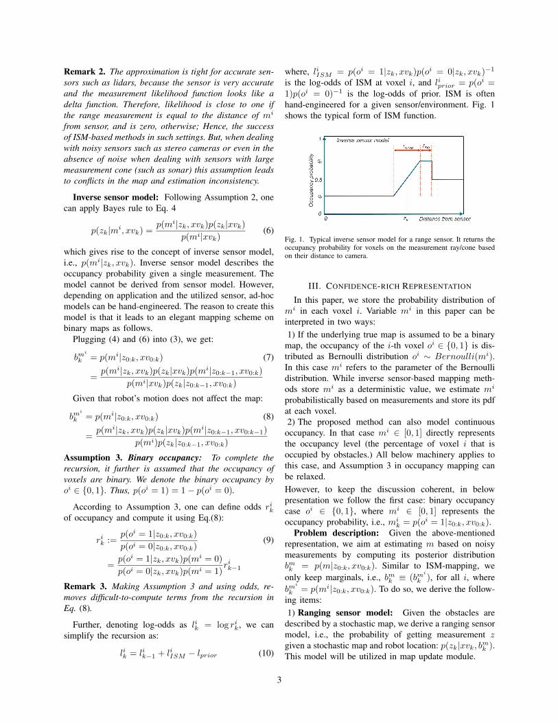
is the log-odds of ISM at voxel i, and liprior = p(oi =1)p(oi = 0)−1 is the log-odds of prior. ISM is oftenhand-engineered for a given sensor/environment. Fig. 1shows the typical form of ISM function.

Fig. 1. Typical inverse sensor model for a range sensor. It returns theoccupancy probability for voxels on the measurement ray/cone basedon their distance to camera.

III. CONFIDENCE-RICH REPRESENTATION

In this paper, we store the probability distribution ofmi in each voxel i. Variable mi in this paper can beinterpreted in two ways:1) If the underlying true map is assumed to be a binary

map, the occupancy of the i-th voxel oi ∈ {0, 1} is dis-tributed as Bernoulli distribution oi ∼ Bernoulli(mi).In this case mi refers to the parameter of the Bernoullidistribution. While inverse sensor-based mapping meth-ods store mi as a deterministic value, we estimate mi

probabilistically based on measurements and store its pdfat each voxel.2) The proposed method can also model continuous

occupancy. In that case mi ∈ [0, 1] directly representsthe occupancy level (the percentage of voxel i that isoccupied by obstacles.) All below machinery applies tothis case, and Assumption 3 in occupancy mapping canbe relaxed.However, to keep the discussion coherent, in belowpresentation we follow the first case: binary occupancycase oi ∈ {0, 1}, where mi ∈ [0, 1] represents theoccupancy probability, i.e., mi

k = p(oi = 1|z0:k, xv0:k).Problem description: Given the above-mentioned

representation, we aim at estimating m based on noisymeasurements by computing its posterior distributionbmk = p(m|z0:k, xv0:k). Similar to ISM-mapping, weonly keep marginals, i.e., bmk ≡ (bm

i

k ), for all i, wherebm

i

k = p(mi|z0:k, xv0:k). To do so, we derive the follow-ing items:1) Ranging sensor model: Given the obstacles are

described by a stochastic map, we derive a ranging sensormodel, i.e., the probability of getting measurement zgiven a stochastic map and robot location: p(zk|xvk, bmk ).This model will be utilized in map update module.

3

2) Recursive density mapping: We derive a recursivemapping scheme τ that updates the current density mapbased on the last measurements

bmi

k+1 = τmi

(bmk , zk+1, xvk+1) (11)

The fundamental difference with ISM-mapping is thatthe evolution of the i-th voxel depends on other voxelsas well. Note that the input argument to τm

i

is the fullmap bm, not just the i-th voxel map bm

i

.3) Motion planning and active perception in density

maps: While planning is beyond the scope of thismethod, we briefly discuss how planning can benefit fromthis enriched map data, to generate actions that activelyreduce uncertainty on the map and leads to safer paths.

π∗ = arg minΠJ(xk, b

mk , π) (12)

Overall, this method relaxes Assumptions 2 and 3 ofthe ISM-based mapping.

IV. RANGE-SENSOR MODELING

In this section, we model a range sensor when theenvironment representation is a stochastic map. We focuson passive ranging sensors like stereo cameras, but thediscussion can easily be extended to active sensors too.

Ranging pixel: Let us consider an array of rangingsensors (e.g., disparity pixels). We denote the cameracenter by x, the 3D location of the i-th pixel by v,and the ray emanating from x and passing through vby xv = (x, v). Let r denote the distance between thecamera center and the closest obstacle to the cameraalong ray xv. In stereo camera range r is related to themeasured disparity z as:

z = r−1fdb (13)

where, f is camera’s focal length and db is the baselinebetween two cameras on the stereo rig. In the following,we focus on a single pixel v and derive the forward sensormodel p(z|xv, bm).

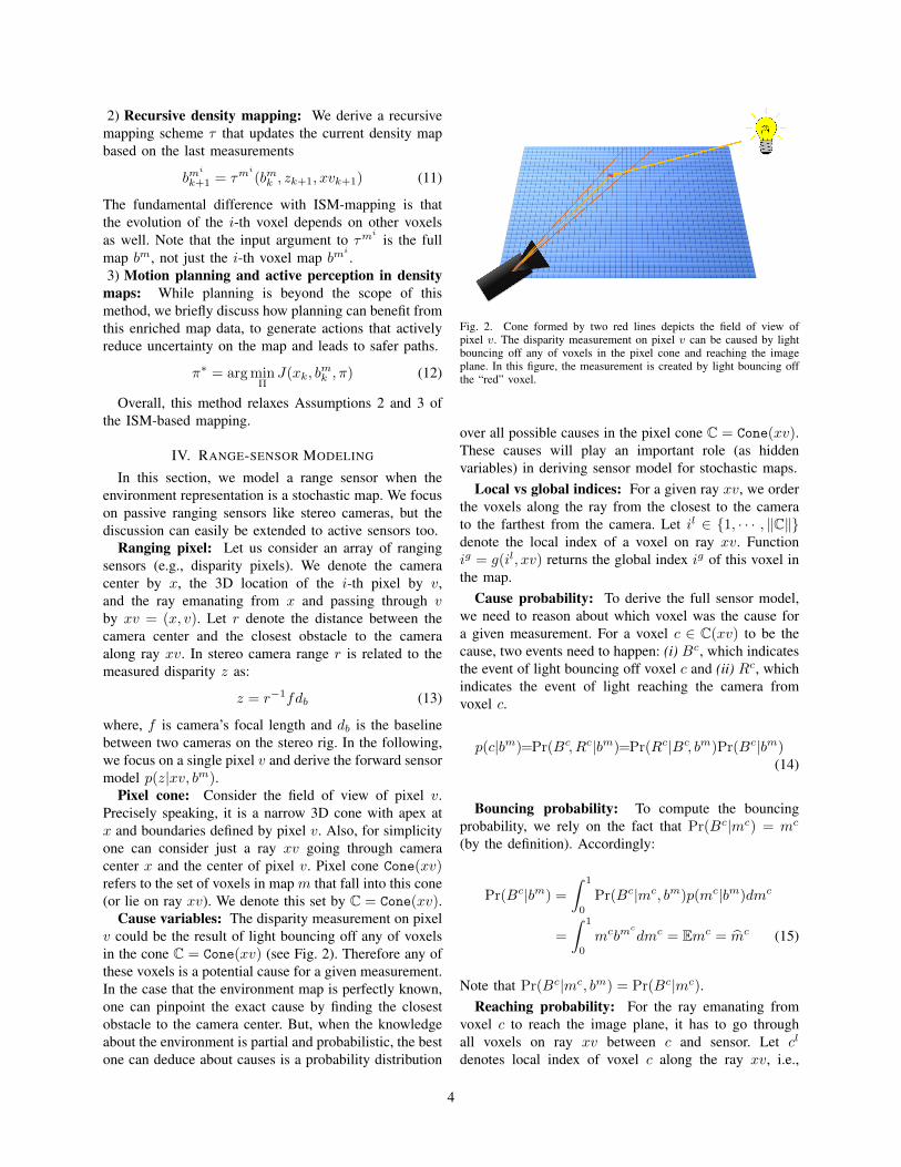
Pixel cone: Consider the field of view of pixel v.Precisely speaking, it is a narrow 3D cone with apex atx and boundaries defined by pixel v. Also, for simplicityone can consider just a ray xv going through cameracenter x and the center of pixel v. Pixel cone Cone(xv)refers to the set of voxels in map m that fall into this cone(or lie on ray xv). We denote this set by C = Cone(xv).

Cause variables: The disparity measurement on pixelv could be the result of light bouncing off any of voxelsin the cone C = Cone(xv) (see Fig. 2). Therefore any ofthese voxels is a potential cause for a given measurement.In the case that the environment map is perfectly known,one can pinpoint the exact cause by finding the closestobstacle to the camera center. But, when the knowledgeabout the environment is partial and probabilistic, the bestone can deduce about causes is a probability distribution

Fig. 2. Cone formed by two red lines depicts the field of view ofpixel v. The disparity measurement on pixel v can be caused by lightbouncing off any of voxels in the pixel cone and reaching the imageplane. In this figure, the measurement is created by light bouncing offthe “red” voxel.

over all possible causes in the pixel cone C = Cone(xv).These causes will play an important role (as hiddenvariables) in deriving sensor model for stochastic maps.

Local vs global indices: For a given ray xv, we orderthe voxels along the ray from the closest to the camerato the farthest from the camera. Let il ∈ {1, · · · , ‖C‖}denote the local index of a voxel on ray xv. Functionig = g(il, xv) returns the global index ig of this voxel inthe map.

Cause probability: To derive the full sensor model,we need to reason about which voxel was the cause fora given measurement. For a voxel c ∈ C(xv) to be thecause, two events need to happen: (i) Bc, which indicatesthe event of light bouncing off voxel c and (ii) Rc, whichindicates the event of light reaching the camera fromvoxel c.

p(c|bm)=Pr(Bc, Rc|bm)=Pr(Rc|Bc, bm)Pr(Bc|bm)(14)

Bouncing probability: To compute the bouncingprobability, we rely on the fact that Pr(Bc|mc) = mc

(by the definition). Accordingly:

Pr(Bc|bm) =

∫ 1

0

Pr(Bc|mc, bm)p(mc|bm)dmc

=

∫ 1

0

mcbmc

dmc = Emc = m̂c (15)

Note that Pr(Bc|mc, bm) = Pr(Bc|mc).Reaching probability: For the ray emanating from

voxel c to reach the image plane, it has to go throughall voxels on ray xv between c and sensor. Let cl

denotes local index of voxel c along the ray xv, i.e.,

4

cl = g−1(c, xv), then we have:

Pr(Rc|Bc, bm) (16)

=(1−Pr(Bg(cl−1,xv)|bm))Pr(Rg(cl−1,xv)|Bg(cl−1,xv),bm)

=

cl−1∏l=1

(1− Pr(Bg(l,xv)|bm)) =

cl−1∏l=1

(1− m̂g(l,xv))

Sensor model with known cause: Assuming thecause voxel for measurement z is known, the forwardsensor is typically modeled as:

z = h(xv, c, nz) = ‖Gc − x‖−1fdb + nz, (17)

where, nz ∼ N (0, R) denotes the observation noise,drawn from a zero-mean Gaussian with variance R. Wecan alternatively describe the observation model in termsof pdfs as follows:

p(z|xv, c) = N (‖Gc − x‖−1fdb, R) (18)

Senosr model with stochastic maps: Sensor modelgiven a stochastic map can be computed by incorporatinghidden cause variables into the formulation:

p(z|xv; bm) =∑

c∈C(xv)

p(z|xv, c; bm) Pr(c|bm) (19)

=∑

c∈C(xv)

N (‖Gc − x‖−1fdb, R)m̂ccl−1∏l=1

(1− m̂g(l,xv))

V. CONFIDENCE-AUGMENTED GRID MAP

In this section, we derive the mapping algorithm thatcan reason not only about the occupancy at each cell,but also about the confidence level of this value. As aresult, it enables efficient prediction of the map that canbe embedded in planning and resulted in safer plans.

We start by a lemma that will be used in derivations.See Appendix A for proof.

Lemma 1. Given the cause, the value of the correspond-ing measurement is irrelevant.

p(mi|ck, z0:k, xv0:k) = p(mi|ck, z0:k−1, xv0:k)

To compute the belief of the i-th voxel, denoted bybm

i

k = p(mi|z0:k, xv0:k), we bring the cause variablesinto formulation.

bmi

k = p(mi|z0:k, xv0:k) (20)

=∑

ck∈C(xv)

p(mi|ck, z0:k, xv0:k) Pr(ck|z0:k, xv0:k)

=∑

ck∈C(xv)

p(mi|ck, z0:k−1, xv0:k) Pr(ck|z0:k, xv0:k)

=∑

ck∈C(xv)

Pr(ck|mi, z0:k−1, xv0:k)

Pr(ck|z0:k−1, xv0:k)Pr(ck|z0:k, xv0:k)bm

i

k−1

It can be shown that bmk−1 is sufficient statistics [18]for the data (z0:k−1, xv0:k−1) in above terms. Thus, wecan re-write (20) as:

bmi

k =∑

ck∈C(xv)

Pr(ck|mi, bmk−1, xvk)

Pr(ck|bmk−1, xvk)Pr(ck|bmk−1, zk, xvk)bm

i

k−1

(21)

In the following, we make the assumption that the mappdf is sufficient for computing the bouncing probabilityfrom voxel c (i.e., one can ignore voxel i given the restof the map.) Mathematically, for ck 6= i, we assume:

Pr(Bck |mi, bmk−1, xvk)uPr(Bck |bmk−1, xvk)=m̂ck

Note that we still preserve a strong dependence be-tween voxels via the reaching probability. To see thisclearly, let’s expand the numerator p(ck|mi, bmk−1, xvk)in (21) as (we drop xv to unclutter the equations):

p(ck|mi, bmk−1, xvk)=Pr(Bck , Rck |mi, bmk−1, xvk) (22)

= Pr(Bck |mi, bmk−1, xvk) Pr(Rck |Bck ,mi, bmk−1, xvk)

=

m̂ck

∏clk−1l=1 (1− m̂g(l,xv)) if clk < il

mi∏clk−1

l=1 (1− m̂g(l,xv)) if clk = il

m̂ck(∏il−1

l=1 (1− m̂g(l,xv)))

×(1−mi)(∏clk−1

l=il+1(1− m̂g(l,xv))

) if clk > il

The denominator is p(ck|bmk−1, xvk) = m̂ck∏clk−1

l=1 (1 −m̂g(l,xv)) for all ck ∈ C(xv). In these equations, clk =g−1(ck, xvk) and il = g−1(i, xvk) are the correspondingindices of ck and i in the local frame.

Therefore, the ratio in (21) is simplified to:

Pr(ck|mi, bmk−1, xvk)

Pr(ck|bmk−1, xvk)=

1 if clk < il

mi(m̂i)−1 if clk = il

(1−mi)(1− m̂i)−1 if clk > il

Plugging the ratio back into the (21), and collectinglinear and constant terms, we can show that:

p(mi|z0:k, xv0:k)

= (αimi + βi)p(mi|z0:k−1, xv0:k−1) (23)

where

αi =

il−1∑clk=1

Pr(ck|bmk−1, zk, xvk)

+ (1− m̂i)−1

|C(xv)|∑clk=il+1

Pr(ck|bmk−1, zk, xvk) (24)

βi = (m̂i)−1 Pr(ck|bmk−1, zk, xvk)

− (1− m̂i)−1

|C(xv)|∑clk=il+1

Pr(ck|bmk−1, zk, xvk) (25)

5

In a more compact form, we can rewrite Eq. (23) as:

bmi

k+1 = τ i(bmk , zk+1, xvk+1). (26)

Sensor cause model: The proposed machin-ery gives rise to the term Pr(ck|z0:k, xv0:k) =Pr(ck|bmk−1, zk, xvk), which is referred to as “SensorCause Model (SCM)” in this paper. As opposed to theinverse sensor model in traditional mapping that needsto be hand-engineered, the SCM can be derived from theforward sensor model in a principled way as follows.

Pr(ck|z0:k, xv0:k) = Pr(ck|bmk−1, zk, xvk) (27)

=p(zk|ck, xvk) Pr(ck|bmk−1, xvk)

p(zk|bmk−1, xvk)

= η′p(zk|ck, xvk) Pr(ck|bmk−1, xvk)

= η′p(zk|ck, xvk)m̂ckk−1

clk−1∏j=1

(1− m̂g(j,xv)k−1 ),∀ck ∈ C(xvk)

where η′ is the normalization constant.

A. Confidence in Map

A crucial feature of the proposed method is that inaddition to most likely map, it provides the uncertaintyassociated with the returned value. In doing so, it in-corporates the full forward sensor model into the map-ping process. In other words, it can distinguish betweentwo voxels, where both reported as almost free (e.g.,m̂1 = m̂2 = 0.1), but one with high confidence andthe other one with low confidence (e.g., σm1

= 0.01 andσm2

= 0.2). This confidence level is a crucial piece ofinformation for the planner. Obviously the planner eitherhas to avoid m2 since the robot is not sure if m2 isactually risk free (due to high variance), or the plannerneeds to take active perceptual actions and take anothermeasurement from m2 before taking an action.

In the ISM-based method only one number is storedin the map, namely the parameter of the Bernoulli dis-tribution. One might try to utilize the variance of theBernoulli distribution to infer about the confidence inan ISM-based map, but due to the incorrect assumptionsmade in the mapping process and also since the Bernoullidistribution is a single parameter distribution (mean andvariance are dependent), the computed variance is not areliable confidence source.

It is very important to note that generally a plannercan cope with large errors “if” there is a high varianceassociated with it. But, if the error is high, and at the sametime, filter is confident about its wrong estimate, planningwould be very challenging, and prone to failure. Toquantify the inconsistency between the error and reportedvariances in the results section, we utilize below measure:

Ic =∑c

ramp(|ec| − 2σc) (28)

where, ec and σc, respectively, denote the estimation errorand variance of voxel c. The ramp function ramp(x) :=max(0, x) ensures that only inconsistent voxels (withrespect to 2σ) contribute to the summation. Accordingly,Ic indicates how much of the error signal is out of bound(i.e., how unreliable the estimate is) over the whole map.We will compute this measure for different maps in theSection VII.

VI. PLANNING WITH CONFIDENCE-AWARE MAPS

In this section, we describe the planning method thatutilizes the confidence-rich representation proposed in theprevious section.

The objective in planning is to get to the goal point,while avoiding obstacles (e.g., minimizing collision prob-ability). To accomplish this, the planner needs to reasonabout the acquisition of future perceptual knowledge andincorporate this knowledge in planning. An importantfeature of the confidence-right map is that it enablesefficient prediction of the map evolution and map un-certainty.

Future observations: However, reasoning about fu-ture costs, one needs to first reason about future ob-servations. The precise way of incorporating unknownfuture observations is to treat them as random variablesand compute their future pdf. But, a common practice inbelief space planning literature is to use the most likelyfuture observations as the representative of the futureobservations to reason about the evolution of belief. Letus denote the most likely observation at the n-th step by:

zmln = arg max

zp(z|bmn , xvn) (29)

Future map beliefs: Accordingly, we can computemost likely future map beliefs:

bmi,ml

n+1 = τ i(bm,mln , zml

n+1, xvn+1), n ≥ k (30)

where, bmi,ml

k = bmi

k .Path cost: To assign a cost J(xk, b

mk , path) to a given

path path = (xvk, uk, xvk+1, uk+1, · · · , xvN ) startingfrom xvk, when map looks like bmk , one needs to predictthe map belief along the path via (30). Assuming anadditive cost we can get the path cost by adding up one-step costs:

J(xk, bmk , path) =

N∑n=k

c(bm,mln , xvn, un) (31)

where the cost in belief space is induced by an underlyingcost in the state space, i.e.,

c(bm,mln , xvn, un)

=

∫c(mn, xvn, un; bm,ml

n )bm,mln (mn)dmn (32)

6

One-step cost: The underlying one-step costc(mn, xvn, un; bm,ml

n ) depends on the application inhand. For safe navigation with grid maps, we use thefollowing cost function:

c(m,xv, u; bm) = mj + (mj − m̂j)2 (33)

where, j is the index of the cell, the robot is at. In otherwords, x ∈ mj .

As a result the cost in belief space will be:

c(bmn , xvn, un) = m̂jn + σ(mj

n)

= E[mjn|zk+1:n, xvk+1:n, b

mk ]

+ Var[mjn|zk+1:n, xvk+1:n, b

mk ] (34)

above observations are ”future observation”.Path planning: To generate the plan we use the

RRT method [19] to create a set of candidate trajectoriesΠ = {pathi}. For each trajectory, we compute the costc(pathi) and pick the path with minimum cost.

path∗ = arg minΠJ(xk, b

mk , path) (35)

VII. RESULTS: PROPOSED MAPPING METHOD

In this section, we demonstrate the performance theproposed mapping method and compare it with thecommonly used log-odds based grid mapping. We startby studying the mapping error and then we discuss theconsistency the estimation process in both methods.

Figure 3(a) shows an example ground truth map. Eachvoxel is assumed to be a square with 10cm side length.The environment size is 2m-by-2m, consisting of 400voxels. Each voxel is either fully occupied (shown inblack) or empty (white). We randomly populate thevoxels by 0 and 1’s, except the voxels in the vicinityorigin, which are set to be free in this example, tobetter test the mapping method. The robot’s (x, y, θ)position has been set to (0, 0, π/2). The robot orientationis changing with a fixed angular velocity of 15 degreesper second. We run simulations for 50 seconds, almostequivalent to two full turns.

For the sensing system, we have simulated a simplestereo camera in 2D. The range of the sensor is 1 meter,with a field of view of 28 degrees. There are 15 pixelsalong the simulated image plane. Measurement frequencyis 10Hz. The measurement noise is assumed to be a zero-mean Gaussian with variance 0.04.

For the ISM-based mapping, we use a typical in-verse sensor model as seen in Fig. 1, with parametersrramp = 0.1, rtop = 0.1, ql = 0.45, and qh = 0.55.The map resulted from the ISM-based mapping andfrom the proposed method are shown in Fig. 3(b) and3(c), respectively. Note that while the inverse sensormodel needs to be hand-tuned for the log-odds-basedmapping, in the proposed mapping methods, there areno parameters for tuning.

To quantify the difference between the maps resultedfrom the log-odds and the proposed method, we computethe error between the mean of estimated occupancy andthe ground truth map, in both ISM and the proposedmapping method. Then we sum the absolute value ofthe error over all voxels in the map as an indicatorof map quality. Fig. 3(d) depicts the evolution of thisvalue over time. As it can be seen from this figure,the proposed method shows less error than the log-odds method, and the difference is growing as moreobservations are obtained.

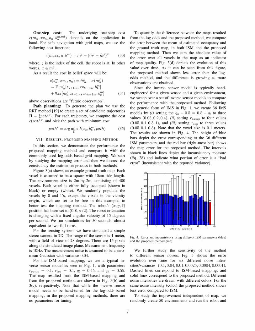
Since the inverse sensor model is typically hand-engineered for a given sensor and a given environment,we sweep over a set of inverse sensor models to comparethe performance with the proposed method. Followingthe generic form of IMS in Fig. 1, we create 36 IMSmodels by (i) setting the qh − 0.5 = 0.5 − ql to threevalues (0.05, 0.2, 0.4), (ii) setting rramp to four values(0.05, 0.1, 0.3, 1), and (iii) setting rtop to three values(0.05, 0.1, 0.3). Note that the voxel size is 0.1 meters.The results are shown in Fig. 4. The height of bluebars depict the error corresponding to the 36 differentISM parameters and the red bar (right-most bar) showsthe map error for the proposed method. The intervalsshown in black lines depict the inconsistency measure(Eq. 28) and indicate what portion of error is a “baderror” (inconsistent with the reported variance).

Fig. 4. Error and inconsistency using different ISM parameters (blue)and the proposed method (red)

We further study the sensitivity of the methodto different sensor noises. Fig. 5 shows the errorevolution over time for six different noise inten-sities/variances (0.1, 0.04, 0.01, 0.0025, 0.0004, 0.0001).Dashed lines correspond to ISM-based mapping, andsolid lines correspond to the proposed method. Differentnoise intensities are drawn with different colors. For thesame noise intensity (color) the proposed method showsless error compared to ISM.

To study the improvement independent of map, werandomly create 50 environments and run the robot and

7

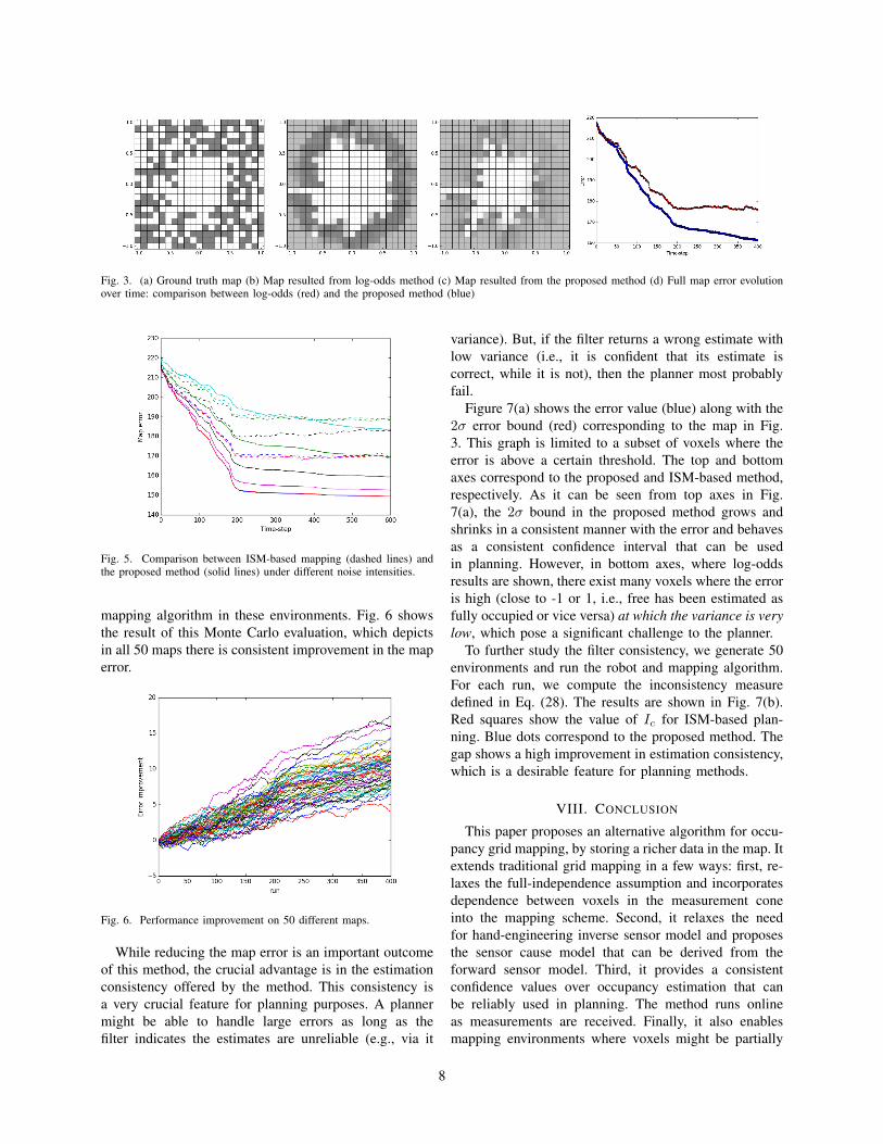
Fig. 3. (a) Ground truth map (b) Map resulted from log-odds method (c) Map resulted from the proposed method (d) Full map error evolutionover time: comparison between log-odds (red) and the proposed method (blue)

Fig. 5. Comparison between ISM-based mapping (dashed lines) andthe proposed method (solid lines) under different noise intensities.

mapping algorithm in these environments. Fig. 6 showsthe result of this Monte Carlo evaluation, which depictsin all 50 maps there is consistent improvement in the maperror.

Fig. 6. Performance improvement on 50 different maps.

While reducing the map error is an important outcomeof this method, the crucial advantage is in the estimationconsistency offered by the method. This consistency isa very crucial feature for planning purposes. A plannermight be able to handle large errors as long as thefilter indicates the estimates are unreliable (e.g., via it

variance). But, if the filter returns a wrong estimate withlow variance (i.e., it is confident that its estimate iscorrect, while it is not), then the planner most probablyfail.

Figure 7(a) shows the error value (blue) along with the2σ error bound (red) corresponding to the map in Fig.3. This graph is limited to a subset of voxels where theerror is above a certain threshold. The top and bottomaxes correspond to the proposed and ISM-based method,respectively. As it can be seen from top axes in Fig.7(a), the 2σ bound in the proposed method grows andshrinks in a consistent manner with the error and behavesas a consistent confidence interval that can be usedin planning. However, in bottom axes, where log-oddsresults are shown, there exist many voxels where the erroris high (close to -1 or 1, i.e., free has been estimated asfully occupied or vice versa) at which the variance is verylow, which pose a significant challenge to the planner.

To further study the filter consistency, we generate 50environments and run the robot and mapping algorithm.For each run, we compute the inconsistency measuredefined in Eq. (28). The results are shown in Fig. 7(b).Red squares show the value of Ic for ISM-based plan-ning. Blue dots correspond to the proposed method. Thegap shows a high improvement in estimation consistency,which is a desirable feature for planning methods.

VIII. CONCLUSION

This paper proposes an alternative algorithm for occu-pancy grid mapping, by storing a richer data in the map. Itextends traditional grid mapping in a few ways: first, re-laxes the full-independence assumption and incorporatesdependence between voxels in the measurement coneinto the mapping scheme. Second, it relaxes the needfor hand-engineering inverse sensor model and proposesthe sensor cause model that can be derived from theforward sensor model. Third, it provides a consistentconfidence values over occupancy estimation that canbe reliably used in planning. The method runs onlineas measurements are received. Finally, it also enablesmapping environments where voxels might be partially

8

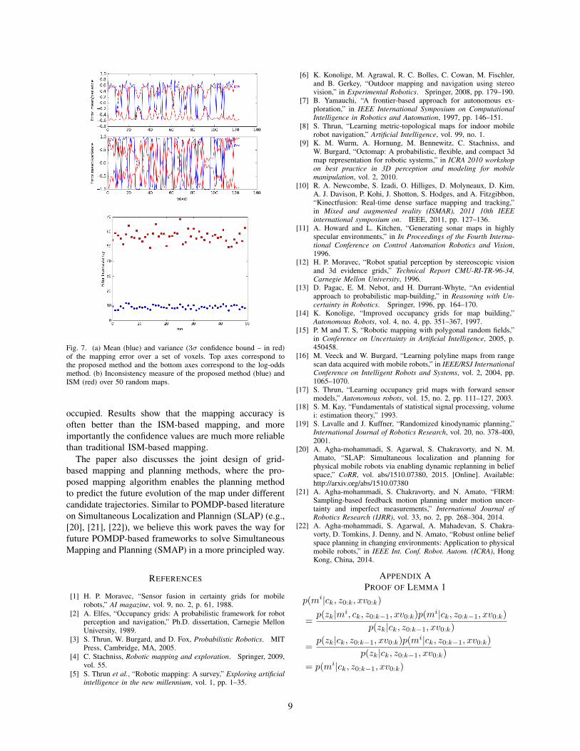
Fig. 7. (a) Mean (blue) and variance (3σ confidence bound – in red)of the mapping error over a set of voxels. Top axes correspond tothe proposed method and the bottom axes correspond to the log-oddsmethod. (b) Inconsistency measure of the proposed method (blue) andISM (red) over 50 random maps.

occupied. Results show that the mapping accuracy isoften better than the ISM-based mapping, and moreimportantly the confidence values are much more reliablethan traditional ISM-based mapping.

The paper also discusses the joint design of grid-based mapping and planning methods, where the pro-posed mapping algorithm enables the planning methodto predict the future evolution of the map under differentcandidate trajectories. Similar to POMDP-based literatureon Simultaneous Localization and Plannign (SLAP) (e.g.,[20], [21], [22]), we believe this work paves the way forfuture POMDP-based frameworks to solve SimultaneousMapping and Planning (SMAP) in a more principled way.

REFERENCES

[1] H. P. Moravec, “Sensor fusion in certainty grids for mobilerobots,” AI magazine, vol. 9, no. 2, p. 61, 1988.

[2] A. Elfes, “Occupancy grids: A probabilistic framework for robotperception and navigation,” Ph.D. dissertation, Carnegie MellonUniversity, 1989.

[3] S. Thrun, W. Burgard, and D. Fox, Probabilistic Robotics. MITPress, Cambridge, MA, 2005.

[4] C. Stachniss, Robotic mapping and exploration. Springer, 2009,vol. 55.

[5] S. Thrun et al., “Robotic mapping: A survey,” Exploring artificialintelligence in the new millennium, vol. 1, pp. 1–35.

[6] K. Konolige, M. Agrawal, R. C. Bolles, C. Cowan, M. Fischler,and B. Gerkey, “Outdoor mapping and navigation using stereovision,” in Experimental Robotics. Springer, 2008, pp. 179–190.

[7] B. Yamauchi, “A frontier-based approach for autonomous ex-ploration,” in IEEE International Symposium on ComputationalIntelligence in Robotics and Automation, 1997, pp. 146–151.

[8] S. Thrun, “Learning metric-topological maps for indoor mobilerobot navigation,” Artificial Intelligence, vol. 99, no. 1.

[9] K. M. Wurm, A. Hornung, M. Bennewitz, C. Stachniss, andW. Burgard, “Octomap: A probabilistic, flexible, and compact 3dmap representation for robotic systems,” in ICRA 2010 workshopon best practice in 3D perception and modeling for mobilemanipulation, vol. 2, 2010.

[10] R. A. Newcombe, S. Izadi, O. Hilliges, D. Molyneaux, D. Kim,A. J. Davison, P. Kohi, J. Shotton, S. Hodges, and A. Fitzgibbon,“Kinectfusion: Real-time dense surface mapping and tracking,”in Mixed and augmented reality (ISMAR), 2011 10th IEEEinternational symposium on. IEEE, 2011, pp. 127–136.

[11] A. Howard and L. Kitchen, “Generating sonar maps in highlyspecular environments,” in In Proceedings of the Fourth Interna-tional Conference on Control Automation Robotics and Vision,1996.

[12] H. P. Moravec, “Robot spatial perception by stereoscopic visionand 3d evidence grids,” Technical Report CMU-RI-TR-96-34,Carnegie Mellon University, 1996.

[13] D. Pagac, E. M. Nebot, and H. Durrant-Whyte, “An evidentialapproach to probabilistic map-building,” in Reasoning with Un-certainty in Robotics. Springer, 1996, pp. 164–170.

[14] K. Konolige, “Improved occupancy grids for map building,”Autonomous Robots, vol. 4, no. 4, pp. 351–367, 1997.

[15] P. M and T. S, “Robotic mapping with polygonal random fields,”in Conference on Uncertainty in Artificial Intelligence, 2005, p.450458.

[16] M. Veeck and W. Burgard, “Learning polyline maps from rangescan data acquired with mobile robots,” in IEEE/RSJ InternationalConference on Intelligent Robots and Systems, vol. 2, 2004, pp.1065–1070.

[17] S. Thrun, “Learning occupancy grid maps with forward sensormodels,” Autonomous robots, vol. 15, no. 2, pp. 111–127, 2003.

[18] S. M. Kay, “Fundamentals of statistical signal processing, volumei: estimation theory,” 1993.

[19] S. Lavalle and J. Kuffner, “Randomized kinodynamic planning,”International Journal of Robotics Research, vol. 20, no. 378-400,2001.

[20] A. Agha-mohammadi, S. Agarwal, S. Chakravorty, and N. M.Amato, “SLAP: Simultaneous localization and planning forphysical mobile robots via enabling dynamic replanning in beliefspace,” CoRR, vol. abs/1510.07380, 2015. [Online]. Available:http://arxiv.org/abs/1510.07380

[21] A. Agha-mohammadi, S. Chakravorty, and N. Amato, “FIRM:Sampling-based feedback motion planning under motion uncer-tainty and imperfect measurements,” International Journal ofRobotics Research (IJRR), vol. 33, no. 2, pp. 268–304, 2014.

[22] A. Agha-mohammadi, S. Agarwal, A. Mahadevan, S. Chakra-vorty, D. Tomkins, J. Denny, and N. Amato, “Robust online beliefspace planning in changing environments: Application to physicalmobile robots,” in IEEE Int. Conf. Robot. Autom. (ICRA), HongKong, China, 2014.

APPENDIX APROOF OF LEMMA 1

p(mi|ck, z0:k, xv0:k)

=p(zk|mi, ck, z0:k−1, xv0:k)p(mi|ck, z0:k−1, xv0:k)

p(zk|ck, z0:k−1, xv0:k)

=p(zk|ck, z0:k−1, xv0:k)p(mi|ck, z0:k−1, xv0:k)

p(zk|ck, z0:k−1, xv0:k)

= p(mi|ck, z0:k−1, xv0:k)

9