Embed Size (px)
Citation preview

UNIVERSITÀ DEGLI STUDI DI PADOVA
Facoltà di IngengeriaCorso di Laurea in Ingegneria Informatica
Tesi di Laurea Magistrale
Algorithms for two-dimensional guillotinepacking problems
Relatore:prof. Michele Monaci
Candidato:Alessandro Di Pieri
Luglio 2013

Abstract
Packing problems are a class of optimization problems that require to pack items into containers.The Guillotine Two-Dimensional Packing Problems are a sub-class of these problems, where bothitems and containers are rectangles and with the constraint that every packed item should bepossibly retrieved with a series of vertical and horizontal cuts that divide the container into twoparts without cutting items. Two exact and two heuristic algorithms have been developed in thisthesis, to solve respectively the Guillotine Two-Dimensional Knapsack Problem and the GuillotineTwo-Dimensional Bin Packing Problem. The first problem has the goal to pack some of the itemsinto one bin maximizing the total profit. The second one, on the contrary, has the goal to pack allthe items using the lowest number of bin as possible.


Contents
Abstract ii
List of Figures iv
List of Tables vi
1 Introduction 1
2 Problem Description 32.1 Packing Problems . . . . . . . . . . . . . . . . . . . . . . . . . . . . . . . . . . . . . 32.2 Knapsack Problem . . . . . . . . . . . . . . . . . . . . . . . . . . . . . . . . . . . . 3
2.2.1 One-dimensional Knapsack Problem . . . . . . . . . . . . . . . . . . . . . . 32.2.2 Two-dimensional Knapsack Problem . . . . . . . . . . . . . . . . . . . . . . 42.2.3 2-Staged Knapsack Problem . . . . . . . . . . . . . . . . . . . . . . . . . . . 52.2.4 k-Staged Knapsack Problem . . . . . . . . . . . . . . . . . . . . . . . . . . . 6
2.3 Bin Packing Problem . . . . . . . . . . . . . . . . . . . . . . . . . . . . . . . . . . . 72.4 NP-Hard problems . . . . . . . . . . . . . . . . . . . . . . . . . . . . . . . . . . . . 72.5 Exact and Heuristic Algorithms . . . . . . . . . . . . . . . . . . . . . . . . . . . . . 8
3 Algorithms Description 103.1 Procedure Recursive . . . . . . . . . . . . . . . . . . . . . . . . . . . . . . . . . . . 103.2 UB Martello and Toth . . . . . . . . . . . . . . . . . . . . . . . . . . . . . . . . . . 133.3 Exact Algorithm for G2KP . . . . . . . . . . . . . . . . . . . . . . . . . . . . . . . 143.4 Heuristic algorithms for G2KP and G2BPP . . . . . . . . . . . . . . . . . . . . . . 14
3.4.1 Heuristic G2KP . . . . . . . . . . . . . . . . . . . . . . . . . . . . . . . . . . 143.4.2 Heuristic G2BPP . . . . . . . . . . . . . . . . . . . . . . . . . . . . . . . . . 15
3.5 Exact Algorithm for G2BPP . . . . . . . . . . . . . . . . . . . . . . . . . . . . . . 16
4 Used Tools 184.1 C Programming Language . . . . . . . . . . . . . . . . . . . . . . . . . . . . . . . . 184.2 Eclipse . . . . . . . . . . . . . . . . . . . . . . . . . . . . . . . . . . . . . . . . . . . 204.3 Valgrind . . . . . . . . . . . . . . . . . . . . . . . . . . . . . . . . . . . . . . . . . . 214.4 Gnuplot . . . . . . . . . . . . . . . . . . . . . . . . . . . . . . . . . . . . . . . . . . 23
5 Implementation 265.1 Input File . . . . . . . . . . . . . . . . . . . . . . . . . . . . . . . . . . . . . . . . . 265.2 Organization of Files . . . . . . . . . . . . . . . . . . . . . . . . . . . . . . . . . . . 275.3 Structures . . . . . . . . . . . . . . . . . . . . . . . . . . . . . . . . . . . . . . . . . 28
ii
5.4 Auxiliary Functions . . . . . . . . . . . . . . . . . . . . . . . . . . . . . . . . . . . 295.5 Functions For G2KP . . . . . . . . . . . . . . . . . . . . . . . . . . . . . . . . . . . 305.6 Functions For G2BPP . . . . . . . . . . . . . . . . . . . . . . . . . . . . . . . . . . 355.7 Outputs . . . . . . . . . . . . . . . . . . . . . . . . . . . . . . . . . . . . . . . . . . 36
6 Computational Experiments 386.1 Instances . . . . . . . . . . . . . . . . . . . . . . . . . . . . . . . . . . . . . . . . . 386.2 Packed Area Percentage . . . . . . . . . . . . . . . . . . . . . . . . . . . . . . . . . 396.3 Combo Upper Bound . . . . . . . . . . . . . . . . . . . . . . . . . . . . . . . . . . . 416.4 Performance of G2KP . . . . . . . . . . . . . . . . . . . . . . . . . . . . . . . . . . 436.5 Performance of G2BPP . . . . . . . . . . . . . . . . . . . . . . . . . . . . . . . . . 46
7 Conclusions 48
Bibliography 50
Acknowledgements 52
iii

List of Figures
2.1 Example of solution of Two-dimensional Knapsack Problem . . . . . . . . . . . . . 52.2 Example of 2-staged patterns: a)Not exact and b)exact . . . . . . . . . . . . . . . 62.3 Example of solution of Two-dimensional Guillotine Knapsack Problem . . . . . . . 6
3.1 Procedure Recursive . . . . . . . . . . . . . . . . . . . . . . . . . . . . . . . . . . . 12
4.1 C Logo . . . . . . . . . . . . . . . . . . . . . . . . . . . . . . . . . . . . . . . . . . . 184.2 Eclipse Foundation Logo . . . . . . . . . . . . . . . . . . . . . . . . . . . . . . . . . 204.3 Valgrind Logo . . . . . . . . . . . . . . . . . . . . . . . . . . . . . . . . . . . . . . . 214.4 Example of final report after the use of memcheck with memory leaks . . . . . . . 234.5 Example of final report after the use of memcheck with no memory leaks . . . . . . 234.6 The resulting plot of the packing . . . . . . . . . . . . . . . . . . . . . . . . . . . . 25
v

List of Tables
6.1 Features of instances . . . . . . . . . . . . . . . . . . . . . . . . . . . . . . . . . . . 396.2 Table of results of area percentages . . . . . . . . . . . . . . . . . . . . . . . . . . . 406.3 Table that shows differences between number of packings and times using Combo
or Martello and Toth . . . . . . . . . . . . . . . . . . . . . . . . . . . . . . . . . . . 426.4 Table that shows maximal and minimal percentage of the total elements for which
using Combo at least one packing is cut . . . . . . . . . . . . . . . . . . . . . . . . 436.5 Table that shows performances of procedure Recursive and of exactG2KP . . . . . 456.6 Table that shows average values found by the heuristic algorithm for G2KP . . . . 466.7 Table that shows performances of exactG2BPP . . . . . . . . . . . . . . . . . . . . 47
vi


Chapter 1
Introduction
The following thesis is focused on the packing problems. The main purpose of this work is to studya way to solve these kind of problems, which are computationally very hard to solve.These problems are not only a mere theoretical study, but they have many practical application.Usually the main fields where these techniques are used are packaging, transportation and storageissues. A simple example could be the problem of fill in the best way possible a truck to minimizethe empty space inside and so to minimize the number of times it has to bring everything to thedestination.Usually very clever techniques are needed to solve packing problems, in particular enumerationtechniques that must be thought very carefully, otherwise the risk is to have too poor performance,that means a too high computation time that runs the risk of not completing.
Hereafter there is a quick overview on what next chapters will deal with:
• Chapter 2: Problem Description: In this chapter all the typologies of problems andalgorithms touched by this work will be explained in more detail. So there will be first ageneral description on what Packing problems are; the attention will be then focused on theproblems actually treated, that are Knapsack problem and Bin-Packing problem, considering,in particular, the cases with shelf divisions, of which problems with guillotine cuts are aparticular instance. Eventually there will be an explanation on what NP-Hard problems areand on the difference between exact and heuristic algorithms.
• Chapter 3: Algorithms Description: In this section the algorithms will be very particu-larly explained from a theoretical point of view. In particular the reasons of certain decisionswill be explained.
• Chapter 4: Used Tools: Here it will be discussed more deeply about the tools thathave been necessary to implement the desired algorithms. So there will be a presentationof the C language used to implement the algorithms, a brief description of the integrateddevelopment environment (IDE) Eclipse and an illustration of the two debugging tools used,Valgrind, a very useful framework that helps a lot find memory leak and referencing problemsand Gnuplot, a command-line program that allows you to visualize graphically the outputof the algorithm and that has been useful for logical debugging.
• Chapter 5: Implementation: Here it will be discussed about the implementation of allthe algorithms. In particular the reasons of certain choices will be pointed out, explaining
1

1 – Introduction
also which other choices had been thought or tried and which kind of problems they hadbrought.
• Chapter 6: Tests: In this chapter the computational experiments are described. First thebenchmark of instances from the literature are presented, then the characteristics of machineswhere tests have been performed are illustrated and finally results of tests will be presentedand discussed.
• Chapter 7: Conclusions: In this section the conclusions on the performed work will bedrawn and suggestions for a possible future continuation of the work will be indicated.
2
Chapter 2
Problem Description
2.1 Packing ProblemsPacking problems are a class of optimization problems that require to pack objects into containers.The goal is to either pack a single container as densely as possible by selecting a subset of itemsfrom a given set or pack all objects using as few containers as possible.In packing problems usually the following objects are given:
• Containers, that usually are or mono-dimensional, so they only impose an upper bound onthe maximum weight of the selected items, or a two- or three-dimensional convex region, or,more rarely, they are an infinite space. In the case they are a finite region, depending fromthe type of problem, they can be just one, a finite number or an infinite number.
• A set of items, some or all of which must be packed into one or more containers. The setmay contain different items with given sizes (or just weights in the mono-dimensional case),or a single item of a fixed dimension that can be used repeatedly.
Two-dimensional Case
Usually the packing must be without overlaps between items and other items or the containerwalls. In some variants, the aim is to find the configuration that packs a single container withthe maximal density. More commonly, the aim is to pack all the objects into as few containers aspossible. In some variants the overlapping (of objects with each other and/or with the boundaryof the container) is allowed but should be minimized.When the container size is increased in all directions, the problem becomes equivalent to the prob-lem of packing objects as densely as possible in infinite Euclidean space (an infinite number ofobjects, all with the same shape). This has brought to the study of the most different shapes,starting from the regular ones, arriving to the curved ones.
2.2 Knapsack Problem
2.2.1 One-dimensional Knapsack ProblemThe Knapsack Problem (KP) [4] is probably the most studied and known packing problem.Given a set of items {1,...,n}, to each of those a profit pj and a weight wj are associated and given
3

2 – Problem Description
a knapsack of capacity W, the Knapsack Problem (KP) consists in choosing a subset of object withmaximum profit to insert into the knapsack.This problem has a great importance in all those context where the goal is to load in an optimalway a bin (that could be a camion, a container, a knapsack, etc.) and in finance, where, given afixed budget, it is necessary to select which things to buy. In addition, KP arises as sub-problemin many complex problems; for instance, it turns out to be the pricing problem when columngeneration techniques are used to solve the Bin Packing Problem.Without loss of generality in the model it is possible to suppose that pj , wj and W are positive
integers, with wj < W for each j = 1,...,n and thatn∑
j=1
wj > W
Introducing the following decisional variables:
xj =
{1, if object j-th is selected0, otherwise
it is possible to set an integer linear programming (ILP) model:
z∗ := maxn∑
j=1
pjxj
n∑j=1
wjxj ≤W
0 ≤ xj ≤ 1 integer, j ∈ {1, ..., n}.
The objective function maximize the total profit of the selected items. The capacity constraintimposes that the sum of the weights of the selected items does not exceed the container capacity;finally the xj variables are integer variables with value 0 or 1.It is correct to specify, anyway, that although this model is the most used to represent a KnapsackProblem, this is not the only one. However in this work we will refer to this model.Usually this model is solved with the branch-and-bound technique or, if W is a not too big in-teger, with the dynamic programming. This limitation is due to the fact that using the dynamicprogramming the complexity is O(nW ), which means that Knapsack Problem is solvable pseu-dopolynomial time, because W can be exponential in the input size so the overall running wouldbecome not polynomial.
2.2.2 Two-dimensional Knapsack Problem
The problem considered in this work is not exactly the knapsack problem described by the modelmentioned above. Each item j ∈ N={1,...,n} is a rectangle with height hj , width wj and profit pjoften equal to that item’s area and the container is a sheet with height H and width W.Without loss of generality in the model it is possible to suppose that pj , wj , hj , W and H arepositive integers, with wj < W and hj < H for each j = 1,...,n.Each edge of the items must be packed parallel to an edge of the container. Thus, considering thecase with hj = H for all j ∈ N (or, in the same way, wj = W for all j ∈ N), the problem can be
4

2 – Problem Description
Figure 2.1. Example of solution of Two-dimensional Knapsack Problem
reduced to the mono-dimensional case.
Real-world applications of Two-dimensional knapsack problem (2KP) arise in loading, transporta-tion, resource allocation, just to mention a few.A possible variant of the problem is the possibility of rotate or not the shapes of items by 90°.This can be useful in some applications, because it can allow less waste of material, while in otherit is not possible to use it, because of features of the material or of the desired items. An examplethat allows rotation is the creation of plywood panels, because it makes no difference which wayyou cut them; an example that does not allow rotation, on the other hand, is the marble cutting,because the grains must be followed.In this work only the so-called fixed-orientation (with no rotation) case has been developed.
2.2.3 2-Staged Knapsack Problem
A classical variant on the 2KP is the 2-staged 2KP, in which the maximum number of cuts allowedto obtain each item is fixed to 2 [6]. A cut must be parallel to the edges of the sheet and must gofrom a part to the other of the portion of surface remained after the previous cuts. It also mustnot pass through other items.If a third stage of cutting is allowed only to separate an item from a waste area, this is called thenon-exact case of 2-staged 2KP or 2-staged 2KP with trimming. Otherwise, we have the exact caseof 2-staged 2KP, or 2-staged 2KP without trimming. Because of the particular disposition thatmust have the items in the solution, this type of problem is also called 2KP with shelf divisions.In figure 2.2 it is possible to see examples of not-exact and exact 2-staged 2KP.
In recent years, most of the literature on two-dimensional packing referred to general k -stagedpacking. This constraint (and in particular the constraint with k=2) can make the problem mucheasier than pure 2KP from a computational viewpoint, but it increases a lot the amount of wastedspace in the solution. However, if automatic machines are used for unloading/cutting items andthe sheet is not significantly expensive, it could preferable to look for solutions of this type.
5

2 – Problem Description
(a) (b)
Figure 2.2. Example of 2-staged patterns: a)Not exact and b)exact
2.2.4 k-Staged Knapsack Problem
A more general case is that where the restriction to the maximum number of cuts allowed to unloadeach item is fixed to a given threshold k. In this case the problem is called k-Staged 2KP [3].Because k can assume any value it is possible to consider in this section also the case when norestriction on the number of cuts is present. This is the general case of the two-dimensional guil-lotine knapsack problem (G2KP), which is exactly the case that will be considered in this thesis.
Figure 2.3. Example of solution of Two-dimensional Guillotine Knapsack Problem
This problem can be considered a middle ground between the classic 2KP and the 2-staged 2KP.The real-world application where it is useful is, like the 2-staged 2KP, that of the automatic ma-chines. This kind of problem is not more difficult than pure 2KP, but it finds a solution that can beused by the automatic machine, meanwhile it is harder than 2-staged 2KP from a computational
6

2 – Problem Description
point of view, but decreases significantly the wasted space in the solution.Hence this problem is considered a very good compromise and this is one of the reasons that ledto focus on this kind of problems.
2.3 Bin Packing ProblemGiven a set N = {1,...,n} of items, the k -th with weight wk > 0 and a set M = {1,...,m} ofcontainers (bin), each one with capacity W, the Bin Packing Problem (BPP) requires to insert allthe items into containers observing these constraints:
• each item must be inserted in one bin;
• the total weight of objects inserted in a bin must not be greater that W ;
• the number of bins used must be minimized.
A necessary condition for a feasible solutions is that, for each k ∈ N , wk ≤ W . Under this condi-tion it is always possible to find a feasible solution in the case that m ≥ n. If m < n the problemof verify if a feasible solution exists is NP-Hard. It will be considered only the case with m ≥ n(supposing m as big as necessary).
One-dimensional bin packing (1BPP) is a classic problem with many practical applications relatedto minimization of space. Two possible examples can be placing computer files with specified sizesinto memory blocks of fixed size, or the recording of all of a composer’s music, where the length ofthe pieces to be recorded are the weights and the bin capacity is the amount of time that can bestored on an audio CD.
Again, we consider a generalization of 1BPP that arises when more than one dimension is presentand additional constraints are necessary. This case is the two-dimensional guillotine bin packingproblem (G2BPP), that can be easily derived from the previous case of the knapsack problem.Also for the BPP, in fact, the features of the two-dimensional bin packing problem (2BPP) are thesame of those of 2KP, with the difference of the goal of the problem that always is to minimize thenumber of bins (sheets) to insert all the items (with rectangular shape). The same approach canbe used for 2-staged 2BPP and k-staged 2BPP.
2.4 NP-Hard problemsIn computer science over the years it was necessary to introduce a discipline that determines if acertain problem was solvable or not and how easily it could be solved. The theory of computationis this: it is the branch of computer science that discuss whether and how efficiently problems canbe solved on a model of computation, using an algorithm. This field is divided into three majorbranches: automata theory, computability theory and computational complexity theory.In particular the computational complexity theory studies which are the minimal necessary re-sources (considering above all computational time and memory) needed by a problem to be solved.Thus, problems are classified in different complexity classes, according to the most efficient algo-rithm that is known to solve each problem.Therefore a complexity class is a class that includes a number of different problems having the
7

2 – Problem Description
same resource-based complexity. Usually different classes are defined in this way:set of problems that can be solved by an abstract machine M using O(f(n)) of resource R, wheren is the size of the input.An abstract machine is a theoretical model of a computer. Here the abstract machine that hasbeen decided to be used is the Turing machine.Two of these classes are particularly important: NP and P. NP is the class of decision problemswhose solutions can be determined by a non-deterministic Turing machine in polynomial time; P,otherwise, is the class of decision problems whose solutions can be determined by a deterministicTuring machine in polynomial time.P then is, trivially, just a subset of NP. But NP has another subset of problems, the so-called NP-complete problems, for which no polynomial-time algorithms are known for solving them (althoughthey can be verified in polynomial time). This takes to biggest open question of the complexitytheory, the P = NP problem, which asks whether polynomial time algorithms actually exist forNP-complete and, accordingly, all NP problems.Finally there are the so-called NP-hard problems. This class of problem is not properly a subsetof NP, because its problems don’t necessarily belong to NP; the name derives from the fact thatproblems belonging to this class are at least as hard as the hardest problem in NP. So a problemH is NP-hard if and only if there is a NP-complete problem that can be reduced to H by a deter-ministic Turing Machine in polynomial time.Knapsack Problem and Bin Packing Problem are two examples of NP-hard problems.
2.5 Exact and Heuristic AlgorithmsIn this work an exact algorithm to solve the G2KP has been implemented. An exact algorithm isan algorithm that solves a problem to optimality [12]. For NP-hard problems, anyway, probablyno polynomial time algorithms exist, but it doesn’t mean that it is not possible to find an exactalgorithm.Two examples of techniques that lead to exact algorithms are Branch and Bound and DynamicProgramming.
Branch And Bound
Branch and bound is a general technique for finding optimal solutions of various combinatorialproblems. A branch and bound algorithm consists of a systematic enumeration of all candidatesolutions, from which some of possible candidates are discarded using upper and lower estimatedbounds of the quantity being optimized.This procedure is usually used to maximize or minimize a function. Suppose that the goal is to findthe maximum value for a function f(x), where x ranges over some set S of admissible or candidatesolutions. Branch and bound is a recursive algorithm that performs 3 steps each time it is called:
1. Branching: splitting procedure that returns two or more subset S1,..., Sn whose union it isthe initial set S. All these new subset are children nodes of a tree where their father node isS ;
2. Bounding: procedure that computes upper and lower bounds for the maximum value off(x) within a given subset of S ;
3. Pruning: if the upper bound for some tree node (set of candidates) A is lower than thelower bound for some other node B, then A may be safely discarded from the search.
8

2 – Problem Description
The recursion stops when the current candidate set S is reduced to a single element, or when theupper bound for set S matches the lower bound. Either way, any element of S will be a maximumof the function within S.
Dynamic Programming
Dynamic programming is a method for solving complex problems by breaking them down intosimpler sub-problems. It is applicable to problems exhibiting the properties of overlapping sub-problems (it can be reduced into sub-problems which are reused several times) and optimal sub-structure (an optimal solution can be constructed efficiently from optimal solutions of its sub-problems).The idea behind dynamic programming is quite simple. In general, to solve a given problem, it isnecessary to solve different parts of the problem (sub-problems), then combine the solutions of thesub-problems to reach an overall solution. Often when using a more naive method, many of thesub-problems are generated and solved many times. The dynamic programming approach seeks tosolve each sub-problem only once, thus reducing the number of computations: once the solutionto a given sub-problem has been computed, it is stored. So the next time the same solution isneeded, it is simply looked up. This approach is especially useful when the number of repeatingsub-problems grows exponentially as a function of the input size.Examples of algorithm that can be implemented using dynamic programming are Dijkstra’s algo-rithm for the shortest path problem, Fibonacci sequence, tower of Hanoi, matrix chain multiplica-tion.
Heuristics
Often, however, the determination of the optimal solution of a NP-hard problem may be too costlyin terms of computation time and in some of these cases even the technological development cannot significantly reduce this time. But sometimes these problems are required to be implementedfor a practical application, so it is not possible to wait for dozen years to have the exact result.Moreover often some parameters are just estimates, so it has no sense to try to find the exactsolution of a problem that comes from uncertain values.Therefore the need arises to solve the difficult problems in reasonable computation times sacrificingthe optimality of the solution.It is due to these reasons that heuristic algorithms are important. Literally they are any methodthat finds a solution of the problem. Ideally one would like a heuristic algorithm to be able toalways determine the optimal solution of a problem. But for most of the problems this is not possi-ble. So generally heuristic algorithms are meant to be algorithms that are likely to find reasonablygood solutions in a short time [11].Unfortunately some problems exist for which even heuristic algorithms can not guarantee to finda solution. In these cases heuristic algorithms are able to find an upper bound (if the problem isa minimization problem) or a lower bound (if the problem is a maximization problem).In this thesis some heuristic algorithm have been implemented. They have been used above allwhen the optimal solution was not needed, because it was enough knowing if a solution existed orhaving just a good solution and not necessary the optimal one.
9

Chapter 3
Algorithms Description
In this section the implemented algorithms will be described.Because in this thesis we are dealing with two-dimensional problems, sheets of width W and heightH will be considered. In addition to this a set N={1,...,n} of types of rectangles (called items) isgiven. The j -th type of items contains aj items, each having a width wj , a height hj and a profitpj .
3.1 Procedure Recursive
The goal of this algorithm is to solve the Guillotine Two-dimensional Knapsack Problem (G2KP)[3].It must receive in input a parameter z0, which is a lower bound on the profit of desired solution.This solution will be a subset of items that can be put into the sheet satisfying the constraintsof the problem. In the solution not only the list of these items will be returned, but also theirposition in the sheet, by means of the coordinates of the bottom-left vertex of each selected item,assuming dimensions be labelled from 0 to W and from 0 to H respectively.In general we denote each assignment of a subset of items to the sheet as a feasible packing, so thesolution is a feasible packing with its own profit that is greater than z0. A feasible packing canbe usually represented as a vector with length n, in which each element of the vector defines thenumber of items of that type that are present in the packing: f = [f1, . . . , fn].Procedure Recursive is called with this name because it implicitly enumerates all feasible packingsby recursively dividing the sheet into two parts, so that each of these divisions represents a (eitherhorizontal or vertical) guillotine cut.
As observed by Christofides and Whitlock [1], for any two-dimensional packing problem an opti-mal solution corresponding to a normal pattern exists, i.e. a solution in which any item is packedwith its left edge adjacent either to the right edge of another item or to the left edge of the sheet.Thanks to this result it is possible to consider just vertical cuts that are in correspondence of linearcombinations of widths of the items. The same observation can be done also with horizontal cuts.So these 2 sets are obtained as follows:
W = {x : x =n∑
i=1
wiαi , 1 ≤ x ≤W , 0 ≤ αi ≤ ai , i = 1, ..., n}.
10

3 – Algorithms Description
H = {y : y =n∑
i=1
hiαi , 1 ≤ y ≤ H , 0 ≤ αi ≤ ai , i = 1, ..., n}.
We assume that both W and H are sorted in ascending order and let t = |W| and s = |H|.Given x ∈ W and y ∈ H and the lower bound solution value z0, let F (x, y, z0) be the set of allfeasible packings of the given items into a sheet of size x× y that can produce a profit larger thanor equal to z0 considering their profit plus the profit that could come from a possible packing ofsome of the remained items into the residual area of the sheet.Moreover, given two sets of feasible packings F 1 = {f1, . . . , fk} and F 2 = {f̄1, . . . , ¯fm}, it ispossible to denote by F 1 ⊕ F 2 the so-called pairwise sum of the packings in those two sets:
F 1 ⊕ F 2 := {f i + f̄ j : i = 1, . . . , k, j = 1, . . . ,m}.
Where the sum between two packings is defined as follows: given two feasible packing f =[f1, . . . , fn] and f̄ = [f̄1, . . . , f̄n] a new packing f̂ = f+f̄ is defined int this way: f̂i := min{f+f̄i, ai}(i = 1, . . . , n).Hence, F 1 ⊕ F 2 is the set of packings that can be obtained combining any packing f i ∈ F 1 withany packing f̄ j ∈ F 2.So, thanks to the fact that W and H are ordered, once set F (x1, y1, z0) has been found, alsosets F (x1, y2, z0), F (x1, y3, z0), . . . , F (x1, ys, z0) can be computed and, in a similar way, alsoF (x2, y1, z0), F (x3, y1, z0), . . . , F (xt, y1, z0). Therefore it is possible to notice that each packingf ∈ F (xj , yi, z0) can be computed as the sum of two feasible packings defined for smaller sizes ofthe bin. Thus, knowing F (xi, H, z0) and F (W, yj , z0) for every i = 1, ..., t− 1 and j = 1, ..., s− 1,F (H,W, z0) can be easily found.
For each packing f that is computed for a certain sheet with width x and height y, an upper boundU(f) is computed on the profit obtainable from the knapsack instance with capacity WH − xy,n types of items, the j -th available in aj − fj copies, each with profit pj and weight wjhj . Theupper bound is computed according to a procedure proposed by Martello and Toth [9] that willbe described later (see section 3.2).This calculation is fundamental to determine whether each found packing is really feasible for thesheet x× y or not and this can be easily verified through this simple inequality:
p(f) + U(f) ≥ z0
with p(f) that is given byn∑
i=1
pifi, where with fi the number of items of type i that are in the
packing is meant.If the aforementioned inequality is satisfied the packing is kept, otherwise it is discarded.In addition to this, another control is introduced, that is the control if a packing is maximal or notand allows to discard all the not maximal packings. We say that a feasible packing f is maximalif no further items can be packed into the sheet, i.e. if, for example, a packing f = [0,2,1,0] wasfeasible, then packings like f = [0,2,0,0], f = [0,1,1,0] and f = [0,1,0,0] would not be maximal,because at least one item can be added still obtaining a feasible packing.
11

3 – Algorithms Description
Figure 3.1. Procedure Recursive
Let us take now a closer look on this procedure presented in figure 3.1.First of allW and H are computed like discussed above and F (x0, yi, z0) is initialised to � for eachi from 1 to s.Then we enter in a double loop where all the possible dimensions of the smaller rectangles are con-sidered. Here set S stores the set of all the possible packings that could be feasible for a rectanglexj × yi.After that we enter in an inner loop, which is very important because here the constraint on guil-lotine cuts is implemented. In this cycle, some xq that satisfies two features are considered: theymust be lower than half of the current xj (because in the second half solutions would be repeated)and a xq̄ so that xq + xq̄ = xj must exist. These xq are possible positions where vertical cutscan be placed. All the possible packings found from the pairwise sum between the sets of feasiblepackings in rectangles with the same height yi and width xq and xq̄ are then added to S throughthe union, so that there are no repeated packings.Then the exactly same process is performed for possible horizontal cuts.At the end of these two phases, if there is an item with dimension that is exactly xj × yi, it isadded to S.Finally on each packing in S the two controls mentioned above are performed: the control on the
12

3 – Algorithms Description
reachability of the minimum desired profit z0 and that on the maximality of the packing.At the end of the algorithm the solution of the problem can be found in F (xt, ys, z0).
To find the coordinates of the bottom-left corner of each item in the solution track of the char-acteristics of each cut performed is kept; in this way, a backward search like in a tree structureallows to find out the desired coordinates from the leaves of the tree, that are the sets of feasiblepackings where each item in the solution is inserted into a packing for the first time (that is whena rectangle with the same dimensions of the item is considered).
3.2 UB Martello and Toth
Before describing the algorithm created by Martello and Toth to compute an upper bound (UB)of the knapsack problem, it is necessary to present the algorithm found by Dantzig [2].In Dantzig algorithm first of all it is necessary to order all the items by profit over weight (p/w)ratio. Then the critical object s is searched, that is the first object of the list that can not be
inserted into the container. Formally: s = min{t :t∑
j=1
wj > c}. After this computation the
residual capacity is defined as the capacity of the container that is still free before inserting items:
c̄ = c −s−1∑j=1
wj . Dantzig UB is then the sum of the profits of the items before the critical object
plus part of the profit the critical object, this amount being proportional to the part that could beinserted in the residual capacity. Formally:
UB(Dantzig) =s−1∑j=1
pj + c̄ ps
ws
The algorithm of Martello and Toth [9] starts in the same way of that of Dantzig. First there isthe ordering of items, then there are computations of critical object and residual capacity. At thispoint there are two possibilities: either not choosing the critical object or choosing it.If the critical object is not chosen, the UB is computed like the Dantzig UB but using the itemafter the critical object in the ordered list in its stead:
UB0 = UB(xs = 0) =s−1∑j=1
pj + c̄ ps+1
ws+1
If the critical object is chosen, then the item before it is just partially chosen:
UB1 = UB(xs = 1) =s∑
j=1
pj + (c̄− ws)ps−1
ws−1
Once these two UBs have been computed the algorithm of Martello and Toth states that the max-imum between them is the searched UB:
UB(Martello− Toth) = max(UB0, UB1)
13
3 – Algorithms Description
3.3 Exact Algorithm for G2KP
The previous algorithm is able to find an exact solution for G2KP, but it requires to have a lowerbound on this solution as input, which could assume the most different values and is impossible toknow in advance.To overcome this problem this algorithm has been introduced. We iteratively execute procedureRecursive with different threshold values in order to find the optimal input z0 to have the bestpossible packing.
First of all a heuristic algorithm (that will be described in detail in the next section) is used tofind a reasonable solution zH that is used as lower bound then an upper bound U is also computedusing the exact algorithm by Martello and Toth for 1KP.After these two preliminary computations, we enter in a loop where the procedure Recursive isiteratively called. The lower bound z0 passed as input is updated at the end of each iteration ofthe cycle. For the first time this value z0 coincides with U but then it assumes always values thatare new.At this point there are two possible situations: either the procedure finds (at least) a feasiblepacking or it does not and returns NULL. In this case, we know that the value of z0 is an upperbound on the optimal solution value; thus U is updated. Otherwise, if a feasible packing is found,the procedure Recursive is used again, but this time with threshold z0 + 1 to understand if z0 wasthe optimal value of the solution or it can be improved. If the algorithm returns NULL it meansthat the optimal solution has been found at it is possible to exit the loop. Otherwise it meansthat it is possible to find a better solution, therefore z0 is a lower bound and so it is possible toupdate zH with this value. Moreover z0 is set again equal to U because to update the value of z0
is necessary to start from the upper bound and decrease it.At the end of the cycle z0 is decreased of a value (U − zH)/50. The value 50 has been computedempirically as trade off between the necessity of a fast improvement of the value and the necessityof not finding lower bounds for Recursive that are too small, because in that case a too large num-ber of packings is found during the execution of the algorithm and this slow down the performancea lot, both considering computational time and memory used. Hence we have preferred to use anot too big decrease of U, so that the case where the lower bound must be updated rarely happensand, when it happens, it is with a value that will not be much lower than the optimal solutionvalue. The only contraindication is that in this manner a bigger number of cycles is performed,but, as they have almost all a value of z0 that is an upper bound on the solution, less packings arefound during the execution of Recursive so it computes faster.
3.4 Heuristic algorithms for G2KP and G2BPP
These algorithms try to find the best possible packing, which will not be necessarily the optimalone; they return respectively the profit of the best packing found and the minimum number of binsnecessary to pack items.
3.4.1 Heuristic G2KP
In this algorithm items are no more divided by type, here each one is considered separately fromthe others. So first of all, just for the first time, they are all ordered by profit over weight.
14

3 – Algorithms Description
Then we enter in a loop that is performed a fixed number of times and can not be terminatedbefore. In this cycle there is another loop inside, where the first k items are considered, such thatthe sum of their profit is better than the actual best profit and that their total area is smaller thanthe area of the container. If the desired list of items does not respect one of the two constraint thecycle is performed again, for maximum a fixed (and low) number of times.When exited from the inner loop, if no set of items is returned no computations are made. Oth-erwise these items are tried to be inserted in the container with a strategy that has been called"MixedStrategy". Two versions of this have been created. These differ from each other just becauseone begins with a vertical shelf while the other with a horizontal one. This has been made becausesome times items can be packed in a way and not in the other. So in the heuristic algorithm firstthe vertical strategy is tried and then, if it does not work, also the horizontal one is tested. If apacking is found the variable containing the best profit is updated and the cycle starts again withthe items in the same order (because it could be possible to add another item and obtain again afeasible packing), otherwise all the items are ordered randomly.
The MixedStrategy has been called in this way because it tries to pack items with an algorithmbased on shelves, but with the difference that these are not all horizontal or vertical, but they arealternated. So in the case of the so-called "MixedStrategyV_G2KP" the first shelf that is triedto be filled is vertical, the second one is horizontal, the third vertical again and so on. For the"MixedStrategyH_G2KP" the algorithm works exactly in the same way starting from the hori-zontal one. Each item of the list is tried to be inserted in the first possible shelf of the order. If innone of them it is possible to insert the item, another shelf is opened. If also it is not possible toopen another shelf then it means that a packing for those elements with this strategy does not exist.
3.4.2 Heuristic G2BPP
Like for the previous algorithm, also in this one items are no more divided by type, but each oneis considered separately from the others. Initially, however, they are all ordered not by profit overweight, but by decreasing size of area.After that we enter in a loop where two strategies are performed to compute the total number ofbins that are necessary to pack all the items. Also here these strategies are based on the Mixed-Strategy and differ from each other because of the different direction of the first shelf (verticalagainst horizontal).Here the cycle is repeated until a strategy finds that all the items can be packed in only one binor until the maximum number of times that the loop must be performed is reached (fixed beforethe beginning of the algorithm).
The MixedStrategy works exactly in the same way of the previous for G2KP and the same is alsotrue for "MixedStrategyV_G2BPP" and "MixedStrategyH_G2BPP". The differences are onlythose connected to the different goals of the problems. So the main difference is that here it is notpossible to have a situation where the packing is not feasible: in the worst case, if it is not possibleto open a new shelf in a bin, a shelf in a new bin is opened.For this kind of problem, anyway, it is possible to terminate the computation before the end ofthe algorithm: this strategy receives in input the best solution that has been found until thatmoment and so, if during the execution of the algorithm the i -th bin is open when i is the bestsolution, the algorithm can be terminated because there will not be an improvement on the solution.
15

3 – Algorithms Description
3.5 Exact Algorithm for G2BPP
The exact algorithm to solve G2BPP is based on the branch and bound technique described above(see Martello and Vigo [10]).First of all also here all items are considered separately and no more divided by type and, as forthe Heuristic G2BPP, they are ordered by decreasing size of area.Then we enter in the recursive algorithm that uses branch and bound. It can be considered as atree structure where each level represents an item and, for each level, the nodes of the upper levelhave as many children as the number of bins where it is possible to pack the item that correspondsto this level. This number of children is the current depth in the tree, because it is assumed thateach item can be inserted in all the possibly previous opened bins plus one (so the total numberof nodes for each level is the number of nodes of the upper level times the depth of each level).To check all the possible combination we begin from the root and then we go down through nodeswith a depth first search. In the meanwhile, to avoid visiting all possible nodes, many nodes canbe pruned or, if the best solution has been found, the search can be stopped. Each time that thesearch reaches a leaf (that will be certainly on the last level) it means that a new better solutionis found.
To check if the solution found is the best solution and stop the search, the so-called lower bound2 (LB2) has been used. This can be found in literature and gives a lower bound on the minimumnumber of bins that are necessary to pack all the items. Hence if a solution that is equal to thevalue of LB2 is found, it must be the optimal solution and the algorithm can terminate.To prune some nodes two techniques are used:
1. if the current node should be inserted into a new bin i and the best solution so far is i aswell, that node and all the branches that start from it are pruned, because there would notbe an improvement of the solution if they were visited;
2. if the current item is the same type of item of the previous one (they are ordered by size, soequal items are close to each other), supposing that the previous item has been inserted inthe j -th bin, all nodes that would represent the insertion into bin from 1 to j -1 are pruned,because if it was not possible to insert the previous item there, so it will not be possible toinsert the current one as well (symmetry breaking).
For each node that is not pruned we try to insert the corresponding item into each bin startingfrom the first possible. If the insertion succeeds the algorithm moves down recursively to its firstchild (obviously checking the pruning conditions), otherwise it moves to its left sibling until it isable to insert the element in a bin. If it is not possible to insert this item in any already openedbin a new bin is opened.
To try to insert the current item in a bin four steps are performed, where the first three guaranteesa faster execution of the algorithm:
1. the total area of the items already inserted in the bin summed with the area of the currentitem must be lower than (or equal to) the area of the bin, otherwise it is not possible theinsertion;
2. if LB2, computed on the items already in the bin plus the current one, is greater than 1 itmeans that only one bin is not sufficient to pack all these items and so it is not possible theinsertion;
16

3 – Algorithms Description
3. the heuristic for G2BPP aforementioned is used. If it returns 1 it means that all items canbe packed into just one bin and so the insertion is performed, otherwise nothing can be saidabout it;
4. if the heuristic returns a value greater than 1 the procedure recursive is used. It tries tosolve the G2KP where all items have profit equal to 1 and the desired total profit is the totalnumber of items that are wanted to be packed. If it returns NULL no packing is possible forthese elements in one bin, otherwise the insertion is performed.
17
Chapter 4
Used Tools
4.1 C Programming Language
Figure 4.1. C Logo
C is a general-purpose programming language [5]. Initially it was associated with the UNIX system,within which it was developed, because both the system and many of its programs were writtenwith C. Anyway this language is not constrained to any machine or operative system, in fact justas effectively it has been used to create primary utilities in different fields.Many basic ideas of C come from BCPL language, but its influence has been mitigated by thelanguage B, created by Ken Thompson in 1970.An important difference, anyway, is that BPCL and B are languages with the absence of types,while C owns a wide range of them. The fundamental types (primitive types) are characters, inte-ger numbers and decimal numbers. Also some derived types exist, created with pointers, vectors,structures and unions. Pointers give rise to an arithmetic of addresses that is independent fromthe machine.C provides the basic constructs to regulate the flow of control, constructs required for the develop-ment of well-structured programs: instructions grouping, the implementation of decisions (if-else),the choice of one among the possible cases (switch), the use of a cycle with a stopping conditionat the beginning (while, for) or at the end (do), the early exit from a cycle (break).Values returned from functions can be both primitive or derived types. Any function can becalled recursively. Local variables are typically "automatic" or created from scratch at each call.
18

4 – Used Tools
Functions of a same program can be divided in different files, called "source files", which must becompiled separately. Variables can be internal to a function, external but visible only within agiven source file, or visible in the entire program (global variables).Before the compilation, another phase called "preprocessing" exists. Here macros, which are con-ventional abbreviations, are substituted with their effective values in the program and other sourcefiles can be included.
C is considered a relatively "low level" language. This definition means that C uses the same kindof objects of many computers, like characters, sets, lists, vectors, that can be combined througharithmetical and logical operators used by real machines.C does not provide commands to directly deal with complex objects (like strings, sets, lists, vec-tors). It does not offer specific tools to allocate memory, with the exception of static definitionsand the local stack of functions. Also the garbage collection is not present. This language doesnot even offer input/output functionalities, it has no read or write operations and no incorporatedmethods to access file as well. All these "high level" mechanisms must be performed with appositefunctions, so many implementations of the language provide a reasonably uniform collection ofthese functions.Despite the absence of some features could seem a big lack, the reduced dimension of the languagebrings some benefits, like the fact that C can be easily learned and that a programmer can expectto know and use the whole language.
C was initially developed by Dennis Ritchie between 1969 and 1973. For many years the so-called"Reference Manual" (a first edition of a book about C) represented the definition of C. In 1983,the American National Standards Institute (ANSI) founded a committee in order to arrive to amodern and exhaustive definition of C. At the end of 1988 the result was the so-called standard"ANSI C". It bases on the original reference manual, because one of the goals of the committeewas to assure that most of the already existing programs would remain valid.The biggest change was that the declaration of a function could then contain a description of itsarguments and the syntax of the definition evolved consequently. This change has been very use-ful, because helps compilers to find errors due to arguments that are incoherent with the expectedtypes of the function.Other minor changes has come, like, for example, floating point computation can now be alsoexecuted with single precision.Anyway The standard gave a second relevant contribution that was the definition of a libraryof functions to support C. It included functions to access the operative system (for example toread and write files), to format input and output data, to allocate memory, to manipulate stringsand so on. Some so-called headers allow uniform access to functions declarations and to data types.
C is not a "strongly typed" language, in the sense that it does not adopt an absolutely rigidpolicy of consistency of data types; in its evolution, however, it has strengthened control over thetypes. For example the original version of C tolerated the interchange between pointers and integernumbers, feature that with the new standard has been removed. Now own declarations and explicitconversions are needed. In spite of this, C keeps its originally philosophy, that programmers knowwhat they are doing, it only asks that their intentions are clearly expressed.
19

4 – Used Tools
4.2 Eclipse
Figure 4.2. Eclipse Foundation Logo
Eclipse [13] is a multi-language Integrated Development Environment (IDE) comprising a baseworkspace and an extensible plug-in system for customizing the environment. It is written mostlyin Java. It can be used to develop applications in Java and, by means of various plug-ins, otherprogramming languages including C thanks to the so-called "C Development Tools" (CDT).
The Eclipse Platform uses plug-ins to provide all functionality within and on top of the runtimesystem. A plug-in in Eclipse is a component that provides a certain type of service within thecontext of the Eclipse workbench. Under this point of view Eclipse can also be considered as anextensible platform for building IDEs. The basic mechanism of extensibility in Eclipse is that newplug-ins can add new processing elements to existing plug-ins.This plug-in mechanism is used for the most different branches of computer science. In additionto allow the Eclipse Platform to be extended using other programming languages such as C andPython, the plug-in framework permits the Eclipse Platform to work with typesetting languageslike LaTeX, networking applications such as telnet and database management systems. The plug-inarchitecture supports writing any desired extension to the environment, such as for configurationmanagement. Java and CVS support is provided in the Eclipse SDK, with support for other versioncontrol systems provided by third-party plug-ins.
Brief History
Industry leaders Borland, IBM, MERANT, QNX Software Systems, Rational Software, Red Hat,SuSE, TogetherSoft and Webgain formed the initial eclipse.org Board of Stewards in November2001. By the end of 2003, this initial consortium had grown to over 80 members.On Feb 2, 2004 the Eclipse Board of Stewards announced Eclipse’s reorganization into a not-for-profit corporation. Originally a consortium that formed when IBM released the Eclipse Platforminto Open Source, Eclipse became an independent body that will drive the platform’s evolution tobenefit the providers of software development offerings and end-users. All technology and sourcecode provided to and developed by this fast-growing community is made available royalty-free viathe Eclipse Public License.
Releases
Since 2006, the Foundation has coordinated an annual Simultaneous Release. Each release includesthe Eclipse Platform as well as a number of other Eclipse projects (like, for example, new versions
20

4 – Used Tools
of some plug-ins).So far, each Simultaneous Release has occurred on the fourth Wednesday of June.
At the time of the work the latest released version of the platform was Eclipse 4.2 (Juno project),but on 26 June 2013 the version 4.3 (Kepler project) has been released. The version used, anyway,was Eclipse 3.8, which stands between the 3.7 and 4.2 versions and provides bugfixes for Indigo(3.7 version) and adds Java 7 support. The CDT version used, however, is the 8.1.1, which wasthe latest release at the time.
4.3 Valgrind
Figure 4.3. Valgrind Logo
Valgrind [16] is a GPL’d system for debugging and profiling Linux programs. With Valgrind’s toolsuite the user can automatically detect many memory management and threading bugs, avoidinghours of frustrating bug-hunting, making his programs more stable. He can also perform detailedprofiling to help speeding up his programs.The Valgrind distribution currently includes six production-quality tools: a memory error detector,two thread error detectors, a cache and branch-prediction profiler, a call-graph generating cacheand branch-prediction profiler, and a heap profiler. It also includes three experimental tools: aheap/stack/global array overrun detector, a second heap profiler that examines how heap blocksare used, and a SimPoint basic block vector generator. It is also possible to use Valgrind to buildnew tools.
Features
• Valgrind is Open Source / Free Software, and is freely available under the GNU GeneralPublic License, version 2;
• Valgrind works with all major Linux distributions and since version 3.5 also on Mac OS X.The latest release is the version 3.8.1 that is the one used for this work.
• It is possible to automatically detect many memory management and threading bugs. Thisgives the user confidence that programs will be free of many common bugs.
• Profiling can help find bottlenecks in programs and so speed up them.
• Valgrind has been used for very complex programs (with up to 25 milion lines of code), forany type of software (from games to scientific programs, to business software) and all overthe world (in over 30 countries)
21

4 – Used Tools
• Valgrind works with programs written in any language, but most of all it is aimed at programswritten in C and C++, because programs written in these languages tend to have the mostbugs. However it can, for example, be also used to debug and profile systems written in amixture of languages like Java, Perl, Python, Fortran and many others.
• Valgrind gives 100% coverage of user-space code, even within system libraries. You can evenuse Valgrind on programs for which you don’t have the source code.
Tool Memcheck
The default and most used tool is Memcheck. It is also the tool used for the debugging of thiswork.Memcheck inserts extra instrumentation code around almost all instructions, which keeps track ofthe validity (all unallocated memory starts as invalid or "undefined", until it is initialized into adeterministic state, possibly from other memory) and addressability (whether the memory addressin question points to an allocated, non-freed memory block), stored in the so-called V bits and Abits, respectively. As data is moved around or manipulated, the instrumentation code keeps trackof the A and V bits so they are always correct on a single-bit level.In addition, Memcheck replaces the standard C memory allocator with its own implementation,which also includes memory guards around all allocated blocks (with the A bits set to "invalid").This feature enables Memcheck to detect off-by-one errors where a program reads or writes outsidean allocated block by a small amount. The problems Memcheck can detect and warn about includethe following:
• Use of uninitialized memory;
• Reading/writing memory after it has been freed;
• Reading/writing off the end of malloc’d blocks;
• Memory leaks.
The price of this is lost performance. Programs running under Memcheck usually run much slowerthan running outside Valgrind and use more memory (there is a memory penalty per-allocation).Thus, few developers run their code under Memcheck (or any other Valgrind tool) all the time.They most commonly use such tools either to trace down some specific bug, or to verify there areno latent bugs (of the kind Memcheck can detect) in the code.
The command used to launch Valgrind was the following:valgrind --tool=memcheck --leak -check=yes --max -stackframe =26118672 ./a.out
where –tool=memcheck indicates which tool of Valgrind it is going to be used; the –leak-checkoption turns on the detailed memory leak detector; the –max-stackframe increases the size of thestack to the desired value; the last parameter is the name of the executable program to analyse.
Here below there is an example of what this tool of Valgrind can return:
In figure 4.4 it is possible to see a kind of leak of memory. This happens because after havingallocated dynamic memory in the C code, it has not been deallocated. And this forgetfulnesshas happened two times: for the allocation made in the method recursive and for that made inreadInput. Valgrind also informs of how many bytes of memory has been lost.
22

4 – Used Tools
Figure 4.4. Example of final report after the use of memcheck with memory leaks
Figure 4.5. Example of final report after the use of memcheck with no memory leaks
In figure 4.5, otherwise, it is possible to see what happens if all these forgetfulness have beencorrected. The program informs that all heap blocks have been freed and so no memory leaks arepossible.
4.4 GnuplotGnuplot [14] is a portable command-line driven graphing utility for Linux, OS/2, MS Windows,OSX, VMS, and many other platforms. The source code is copyrighted but freely distributed. Itwas originally created to allow scientists and students to visualize mathematical functions and datainteractively, but has grown to support many non-interactive uses such as web scripting. It is alsoused as a plotting engine by third-party applications like Octave. Gnuplot has been supported and
23

4 – Used Tools
under active development since 1986.
Gnuplot supports many types of plots in either 2D and 3D. It can draw using lines, points, boxes,contours, vector fields, surfaces, and various associated text. It also supports various specializedplot types.
Gnuplot supports many different types of output: interactive screen terminals (with mouse andhotkey input), direct output to pen plotters or modern printers, and output to many file formats(eps, emf, fig, jpeg, LaTeX, pdf, png, postscript, ...). Gnuplot is easily extensible to include newoutput modes. Recent additions include interactive terminals based on wxWidgets (usable onmultiple platforms), and Qt. Mouseable plots embedded in web pages can be generated using thesvg or HTML5 canvas terminal drivers.
The used version is the 4.6.1, which was the latest one at the beginning of the work. At the momentversions till 4.6.3 have been released.
The importance of Gnuplot in this work has been that of "logical debugging". It has been usedto check whether the output of the algorithms were correct or not, printing on the screen the plotrepresenting the resulting packing of rectangular items. To have a better debugging it has beenpossible to set the length of the axes that must be visible in a single window in order to representa single bin.To represent items in the bin, objects Rectangles of the program has been used. To plot them itwas enough to set the coordinates of the bottom left and of the upper right corners. They alsohave been coloured with the command "fillcolor" to avoid confusing them with the empty spacesin the bin, thing that could have happened if the rectangles would have been filled with white asthe background of the bin.Here below there is an example of a file that creates a plot with Gnuplot.
set xrange [0:537]set yrange [0:244]set object rect from 504 ,178 to 534 ,244 fillcolor rgb "#87 cefa"set object rect from 458,0 to 537,89 fillcolor rgb "#87 cefa"set object rect from 458,89 to 537 ,178 fillcolor rgb "#87 cefa"set object rect from 474 ,178 to 504 ,244 fillcolor rgb "#87 cefa"set object rect from 400,90 to 458 ,178 fillcolor rgb "#87 cefa"set object rect from 444 ,178 to 474 ,244 fillcolor rgb "#87 cefa"set object rect from 347,0 to 458,45 fillcolor rgb "#87 cefa"set object rect from 347,45 to 458,90 fillcolor rgb "#87 cefa"set object rect from 414 ,178 to 444 ,244 fillcolor rgb "#87 cefa"set object rect from 120,0 to 236,90 fillcolor rgb "#87 cefa"set object rect from 236,0 to 347,45 fillcolor rgb "#87 cefa"set object rect from 236,45 to 347,90 fillcolor rgb "#87 cefa"set object rect from 212,90 to 400 ,134 fillcolor rgb "#87 cefa"set object rect from 212 ,134 to 400 ,178 fillcolor rgb "#87 cefa"set object rect from 384 ,178 to 414 ,244 fillcolor rgb "#87 cefa"set object rect from 0,66 to 119 ,90 fillcolor rgb "#87 cefa"set object rect from 159,90 to 212 ,147 fillcolor rgb "#87 cefa"set object rect from 168 ,147 to 210 ,178 fillcolor rgb "#87 cefa"set object rect from 256 ,178 to 384 ,244 fillcolor rgb "#87 cefa"set object rect from 90,0 to 120 ,66 fillcolor rgb "#87 cefa"set object rect from 106,90 to 159 ,147 fillcolor rgb "#87 cefa"set object rect from 126 ,147 to 168 ,178 fillcolor rgb "#87 cefa"set object rect from 0,178 to 128 ,244 fillcolor rgb "#87 cefa"
24

4 – Used Tools
set object rect from 128 ,178 to 256 ,244 fillcolor rgb "#87 cefa"set object rect from 60,0 to 90,66 fillcolor rgb "#87 cefa"set object rect from 0,90 to 53,147 fillcolor rgb "#87 cefa"set object rect from 53,90 to 106 ,147 fillcolor rgb "#87 cefa"set object rect from 84 ,147 to 126 ,178 fillcolor rgb "#87 cefa"set object rect from 0,0 to 30,66 fillcolor rgb "#87 cefa"set object rect from 30,0 to 60,66 fillcolor rgb "#87 cefa"set object rect from 0,147 to 42,178 fillcolor rgb "#87 cefa"set object rect from 42 ,147 to 84,178 fillcolor rgb "#87 cefa"
Code 4.1. Gnuplot input file to plot a packing
Figure 4.6. The resulting plot of the packing
25

Chapter 5
Implementation
5.1 Input FileFor the implementation of the problem it has been decided to use as input the same kind of filesthat are used in literature. So they have a very well defined structure, which will be described here.
2040 7031 43 4 50030 41 2 48029 39 4 46028 38 4 44027 37 3 42026 36 4 41025 35 3 40024 34 4 38033 23 4 36022 32 3 34031 21 3 32029 18 3 30017 27 2 28015 24 2 24016 25 4 26015 24 1 24023 14 4 22021 12 3 18019 11 4 1609 17 1 140
Code 5.1. Example of an input file
The structure of the file must be the following:
• on the first row there must be the number of the types of rectangles that are listed in thefollowing lines;
• on the second row there must be the values of the dimensions of the bin. The first numberrepresents the width and the second one stands for the height;
• all the next lines have the same structure and they are exactly the quantity present in thefirst line. For each of these rows the first two numbers represent respectively width and
26
5 – Implementation
height of the rectangle, the third number stands for the number of rectangles that have thatshape and the fourth is the profit that each rectangle with that shape has.
In the example, moreover, rectangles are ordered by profit, but this is not the rule: to have a validinput file it is enough to follow the three points described here above, with no limitations on theorder of rectangles.
5.2 Organization of Files
To make the implementation as readable as possible, the work has been structured following theidea of modularity. So different files have been created for different algorithms and also in the samefile, functions have been programmed using sub-functions to increase readability and because, if asub-function is used more than one time in the main function and there is the desire to modify it,in this manner it is possible to modify only one time the code to change it everywhere.The files that have been implemented are the following:
• structures.h: here all the structs that are needed to represent objects present in this kindof problem are implemented: for example some of them are Sheet, Rectangle, Packing,Container;
• auxiliaryFunctions.h: header file where all the functions present in auxiliaryFunctions.care listed;
• auxiliaryFunctions.c: here all the functions of its header file are implemented. These func-tions are not sub-functions of algorithms to solve G2KP and G2BPP, but they are external.Here there are, for example, the method to parse the input and a method to order rectanglesby profit over weight ratio;
• functionsG2KP.h: header file where all the functions present in functionsG2KP.c are listed;
• functionsG2KP.c: here all the functions of its header file are implemented. These are allthe functions related to G2KP, so those necessary to compute the exact solution of G2KPand the procedure recursive, plus all the related sub-functions;
• functionsG2BPP.h: header file where all the functions present in functionsG2BPP.c arelisted. Here also some struct and some types necessary to use LB2 are defined;
• functionsG2BPP.c: here all the functions of its header file are implemented. These are allthe functions related to G2BPP, therefore that used to compute the exact solution of G2BPPand all its sub-functions, like heuristic functions and branch and bound method;
• main.c: in this file just the main of the program has been implemented where can be decidedto perform G2KP or G2BPP.
In addition to these files other two file called 3dbpp.h and 3dbpp.c [8], which have been imple-mented by David Pisinger [15], are used. These are necessary, because the implementation of LB2is contained within them.
27

5 – Implementation
5.3 StructuresIn these section all the implemented structures are described.To understand why some data types are used instead of others it is important to briefly explainwhat is a struct. A definition of a struct is the same of defining a variable, because both aredefining a limited memory space. The difference is that a struct has inside some fields. Thesefields are not necessarily all of the same size (in terms of memory space). If all the fields have thesame size, then the space used by the structure is the sum of them, otherwise it is a bit different.The size of a struct must be a multiple of the biggest of its fields, so the sum of all of them iscomputed and, if the result is not perfectly a multiple of the biggest element, a padding is used toreach the next multiple.Hereafter the implemented structures are presented:
• Sheet: it represents the bin where items must be packed. It has only two fields of integer,which represent the dimensions, width and height, respectively.
• Rectangle: it represents each item that must be packed. As it is possible to see from thecode, it has five fields that represent respectively width and height of the rectangle, the totalnumber of rectangles that have that shape, the profit of that kind of rectangles and the index,that is the position that it has in the input file from where it has been retrieved.
/∗∗∗ Struc ture t ha t r ep re s en t s r e c t an g l e s∗/
typedef struct r e c t ang l e {
int width ; //width o f the r e c t ang l eint he ight ; // he i gh t o f the r e c t ang l eint number ; //number o f r e c t an g l e s with t h i s s i z eint p r o f i t ; // p r o f i t o f t h i s kind o f r e c t an g l e sint index ; // index o f the r e c t ang l e
} Rectangle ;
Code 5.2. Example of code for a structure
• Shelf : it represents a shelf in the heuristic algorithms. It can be used either as horizontal orvertical shelf thanks to its four fields: the first two determines the width or the height of theshelf, used respectively in the case if the shelf is vertical or horizontal. In the case of verticalshelf, then, to determine if any other packing can still be packed the residualHeight field isused, while for the horizontal there is the residualWidth field. All these fields are integer.
• Bin: it represents the bin in the implementation with shelves inside in the heuristic algo-rithms. It has four fields: a pointer to an array of shelves, where they are saved, an integerthat gives the number of shelves (the length of the array) and other two integers that representresidual height and residual width in the bin.
• Packing: it represents each possible packing of items in the bin. This is the most criticalstructure in terms of memory space used, because the number of packings that might besaved at the same time could be very high. So, above all in this case, it has been tried tominimize the space necessary for each field. Moreover, for each packing has been necessaryto save some information that are used at the end of the algorithm to retrieve the coordinatesof the position of items in the packing. So six fields have been implemented:
28
5 – Implementation
– unsigned char* pack: pointer to an array that represents the packing: each numberrepresents the total number of rectangles with that shape that are in the packing.
– unsigned short k: index of the array W or H where to cut, which is needed to retrievethe position of the first of the two packing, between which the cut has been performed,in the matrix where all packings are saved. If it is a "base case" (which will be betterdefined later), so there is only field element in the packing and can not be cut, it isequal to 0.
– unsigned short q: index of the other packing that brings to the feasible Packing throughthe cut obtained through the pairwise sum; like the previous one if we are in a basecase, it assumes the value 0.
– char direction: it can assume three values: ’W’ if there cut is vertical, ’H’ if the cut ishorizontal, ’0’ if no cut can be performed
– unsigned char positionK: index of the position of the packing in the cell of the matrixfound thanks to the field k.
– unsigned char positionQ: index of the position of the packing in the cell of the matrixfound thanks to the field q.
Hence, the total memory space occupied by this struct is the following: 8 bytes for thepointer, if the architecture of the computer is 64-bit, 1 byte for each of the three chars and2 bytes for each of the two shorts. So the sum is 15 bytes, but, because of the pointer, thestruct occupies 16 bytes, with 1 byte of padding.
• Container: it represents a set of packings. It is used in the matrix where all packings aresaved to represent each cell of the matrix. It has only two fields, which are a pointer to thearray of packing and the length of this array.
• Node: it represent a node of the tree used to retrieve the positions of items in the feasiblepacking, starting from the root and descending to the leaves. There are seven fields. The firstis a pointer to the next packing from where another cut (and consequently 2 sub-packings)can be retrieved. Then w and h are the indexes of the matrix where this packing is saved. xand y are the searched coordinates of the bottom-left vertex. hDx and wDx are the indexesused to set the right child. They are necessary to determine position taking into account alsocuts previously made.
• RectPosition: it represents the position of each item in the feasible packing. It has threefields: the index of the item, the coordinate x of the position and the coordinate y of theposition, all of them are integers.
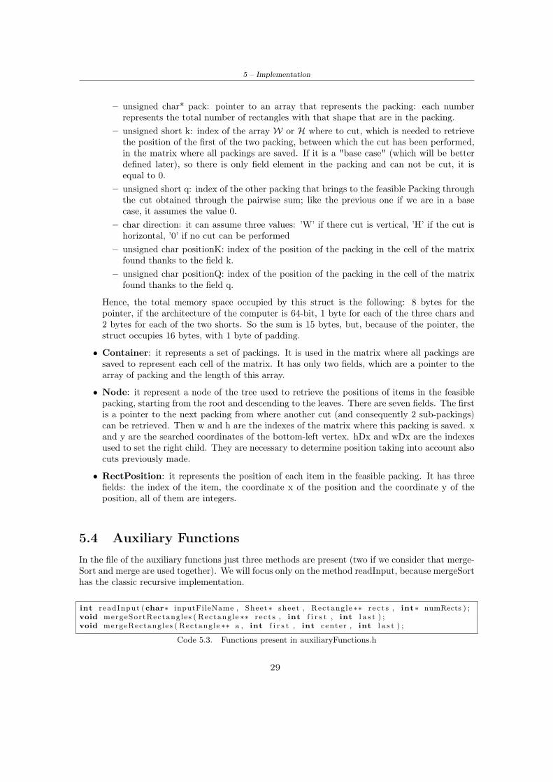
5.4 Auxiliary FunctionsIn the file of the auxiliary functions just three methods are present (two if we consider that merge-Sort and merge are used together). We will focus only on the method readInput, because mergeSorthas the classic recursive implementation.
int readInput (char∗ inputFileName , Sheet ∗ sheet , Rectangle ∗∗ r e c t s , int∗ numRects ) ;void mergeSortRectangles ( Rectangle ∗∗ r e c t s , int f i r s t , int l a s t ) ;void mergeRectangles ( Rectangle ∗∗ a , int f i r s t , int center , int l a s t ) ;
Code 5.3. Functions present in auxiliaryFunctions.h
29

5 – Implementation
readInput, first of all, tries to open the file just in reading mode with the function "fopen" and,if there is any problem, it terminates with an error. Then with some "scanf" information areretrieved from the input file and saved into the correct fields of a Rectangle and each of these isplaced into an array.It has been noticed, however, that some of the input files, even if they were from literature, hadsome of the types of rectangles that were equal to each other, despite being written in differentrows. So in this function a control has been introduced to check if this happens and, in case, tomerge the two types into one.This method returns 0 if the reading was successful, 1 otherwise, and returns also the array ofRectangles and the length of this array, thanks to the fact that it received their addresses as input.
5.5 Functions For G2KPThe list of functions present in functionsG2KP.h has been divided in two parts: in the first partthere are all those related to the function exactG2KP, while in the second there are all those relatedto the procedure recursive.
For the first part first of all we must consider the function exactG2KP. It has been described indetail above and the implementation is really simple, thanks to the modularity of the code. Theonly fact that is particularly interesting to notice is that this function returns not only the list ofthe coordinates of the items in the feasible packing, but also its length and the optimal solutionvalue, thanks to the fact that the input variables optimalSolution and numPackedRects are ad-dressed and so these values are updated directly there and they do not need a return statement.
RectPos i t ion ∗ exactG2KP ( int maxWidth , int maxHeight , int numRects , Rectangle ∗ r e c t s ,int ∗ opt imalSo lut ion , int ∗ numPackedRects ) ;
int heuristicG2KP ( int maxHeight , int maxWidth , int numRects , Rectangle ∗ r e c t s ) ;int mixedStrategyV_G2KP( Rectangle ∗ randomOrder , int numElem , int maxHeight , int maxWidth ) ;int mixedStrategyH_G2KP( Rectangle ∗ randomOrder , int numElem , int maxHeight , int maxWidth ) ;void findRandomOrder ( Rectangle ∗∗ r e c tL i s t , int totRects ) ;void mergeSortRectanglesByNumber ( Rectangle ∗∗ r e c t s , int f i r s t , int l a s t ) ;void mergeRectanglesByNumber ( Rectangle ∗∗ a , int f i r s t , int center , int l a s t ) ;
Code 5.4. Functions present in functionsG2KP.h part 1
Also the heuristicG2KP implementation is quite simple. An auxiliary array of Rectangles rando-mOrder has been introduced where all the randomizations of the items are saved. For the firsttime, where, as mentioned before, all elements should be ordered by profit over weight ratio, itis enough to copy elements from array rects, because they should be already ordered in this way.Then, considering the inner loop, has been decided to proceed in the way described in chapter 3,because in this manner the 2 strategies in the outer cycle are computed only for set of items thatpotentially can improve the best solution value saved at the time.To randomize the order of items has been used the function srand that seeds the random numbergenerator with the input number. The input number is the current time, so it gives a good random-ization. Each random number that is generated is saved in the field "number" of the Rectangles,because they are no more divided by type, so each Rectangle would have value 1 in that field.Then items are ordered with the mergesort by decreasing order of field number.Let us consider now the mixedStrategy functions. We will discuss only the vertical one, becausethe horizontal one is the complementary.First of all this function is characterized by a big external loop that is performed on each Rectangle
30

5 – Implementation
to find the correct Shelf where to pack it. This search is performed starting from the first Shelfand then trying the following. Shelves with even index are considered as vertical (respectively:horizontal), those with odd index are considered as horizontal (vertical) (the first index is zero, soit will start with a vertical one). To check if an item can be packed into a vertical (horizontal)shelf two controls are necessary: its width (height) should be lower than the width (height) of theshelf and its height (width) should be lower than the residualHeight (residualWidth) of the shelf.If these two controls are passed, the residualHeight (residualWidth) is updated decreasing it by theheight of the item. If we arrive to consider the index of a shelf that has not been opened yet, wetry to open it (vertical or horizontal, depending from the index). The control to perform to verifyif it is possible is to check if height and width of the current item are lower than the residual heightand residual width of the bin. These two variables have been initialised at the beginning of thisfunction with the values of the dimensions of the bin and each time a new shelf is opened (passingthe last control mentioned) they are updated. If the shelf is vertical the residual width is decreasedby the item width, otherwise the residual height is decreased by the item height. Moreover, when anew vertical (horizontal) shelf is created, also the width (height) and the residualHeight (residual-Width) of the shelf are set as respectively the width (height) of the current item and the differencebetween the residual height (width) of the bin and the height (width) of the current item. Themethod returns 1 if at the end a packing for each item is found, otherwise it returns 0 if it happensthat the conditions for opening a new shelf can not be met.
Now the procedure recursive and all its sub-functions will be considered.
RectPos i t ion ∗ r e c u r s i v e ( int z0 , int maxWidth , int maxHeight , int numRects ,Rectangle ∗ r e c t s , int ∗ numPackedRects ) ;
void saveDataAndQuantities ( int ∗ value , int ∗ number , int ∗∗ arrayData , int ∗∗ arrayQuantity ,int ∗ s i z e , int ∗ counter ) ;
int ∗ l inearCombinat ion ( int maximum, int ∗∗ arrayData , int ∗∗ arrayQuant i t i e s ,int counterInput , int ∗ counterOutput ) ;
Container pairwiseSum ( Container a , Container b , int numRects , Rectangle ∗ r e c t s , int q ,int cut , char d i r e c t i o n ) ;
Container unionPackingsUB ( Container a , Container b , int numRects , Rectangle ∗ r e c t s ,int maxWidth , int maxHeight , int width , int height , int isLastW ,int isLastH , int z0 ) ;
void mergeSortPackings ( Container ∗pack , int f i r s t , int l a s t , int numRects ) ;void mergeSort ( Packing ∗∗ a , int f i r s t , int l a s t , int numRects ) ;void mergePackings ( Packing ∗∗ a , int f i r s t , int center , int l a s t , int numRects ) ;int ∗ r e s i z eAr r ay In t ( int ∗ array , int ∗ o ldS ize , int newSize ) ;Packing∗ re s i zeArrayPack ing ( Packing∗ array , int ∗ o ldS ize , int newSize ) ;Node∗ res izeArrayNode (Node∗ array , int ∗ o ldS ize , int newSize ) ;RectPos i t ion ∗ res izeArrayRectPos ( RectPos i t ion ∗ array , int ∗ o ldS ize , int newSize ) ;int minVal ( int a , int b ) ;int maxVal ( int a , int b ) ;int f i n dC r i t i c a lOb j e c t ( int pro f i t_j , int area_j , int maxNum_j, int ∗ r e s idua lCapac i ty ,
int previousUpperBound , int ∗ c r i t i ca lOb j ec tFound ) ;int comparePackings (unsigned char∗∗ a , unsigned char∗∗ b , int s i z e ) ;
Code 5.5. Functions present in functionsG2KP.h part 2
It is possible to consider the procedure recursive as divided into three parts: a first part where Wand H are computed, a second part where all possible packings are generated and at the end thefeasible packing, if exists, is found and a third part where the positions of the items in the feasiblepacking are retrieved.In the first part the computation of W and H is pretty simple in the method recursive, becauseall the work is performed by the two auxiliary functions saveDataAndQuantities and linearCom-bination.To compute W saveDataAndQuantities saves into two different arrays all the possible different
31

5 – Implementation
widths of the items and the number of items that have each width. Then it does the same withheights to compute H. To implement this, because of the small size of input, for each element asimple exhaustive search has been used to find the position where to insert it.LinearCombination uses the two arrays computed with saveDataAndQuantities to find W (or Hrespectively). This algorithm will be explained only for the widths, because for the heights it is thecomplementary. First of all an array A is created with length equal to the width of the sheet plusone and it is initialised with all zeros except in the position of index 0 where it is initialised with1. This happens because each cell of the array is considered as a possible dimension and in eachcell is saved the value of the iteration when that dimension is found or zero if it has still not beenfound at that moment. For each element in the input arrays (j ) each element of A (k) is checkedand considered only if it has been computed on the previous iteration. In this case, consideringthe quantity (i) that corresponds to the current element, the new sizes are computed as the linearcombination between the current size k and the dimension corresponding to the index j weightedby the quantities i. To explain it more clearly, it has been computed with the following formula:// I t e r a t e on quan t i t i e sfor ( i = 0 ; i <= (∗ ar rayQuant i t i e s ) [ j −1] ; i++) {
//Compute the valueint value = k + i ∗(∗ arrayData ) [ j −1] ;
}
Code 5.6. Formula for linear combination
After this computation the found value is checked to be lower than the length of A and, if this isthe case, the number of the computation is saved into the cell corresponding to the computed size.At the end of the algorithm all the found sizes are saved into another array that is returned withits size.
Going back to procedure recursive, starting the second part we have W, H and their respectivesizes t and s. The second part is characterized by a double loop on all values of W and H. At theend of each iteration a set of Packings is saved into the correct cell of a matrix t× s of Containers,called F.For the implementation of this part of the algorithm, because the biggest problems were comingfrom the memory space needed to save all the possible packing, we have decided to change a littlethe algorithm to reduce the number of packings that were saved into the matrix. To obtain thisresult the control on the UB of the profit for each packing is performed each time a union must beexecuted.In this part some other variables of type Container have been introduced, because each of themrepresents one set of packing, in the pseudo-code represented with F (x, y, z0). Moreover, whenis computed the Container temp as solution of the pairwise sum, it is ordered with a mergeSortby lexicographical order before performing the union with the Container S containing the packingthat could be insert in the current cell of the matrix, so both S and temp are ordered and it ismuch easier to perform the union.Considering the pairwise sum, to call this function from the recursive procedure, it is necessaryto pass as its input the values of the cut, so the index q found, his complementary index called k(that is the q̄ of the pseudo-code), which is the real position where the cut is performed, and thedirection of the cut, that could be horizontal (’H’) or vertical (’W’). In this method then a doublecycle on all the elements of the two Containers passed as input is performed to find the pairwisesum and, when a packing belonging to it is computed, all the features of the cut are saved as well.Here there is a fragment of code where it can be seen:
32

5 – Implementation
//Cycle on a l l the elements of afor ( l = 0 ; l < a . s i z e ; l++) {
//Cycle on a l l the elements of bfor ( k = 0 ; k < b . s i z e ; k++) {
//Cycle on a l l the components of the f ea sab l e packingsfor ( i = 0 ; i < numRects ; i++) {
int value = a . f [ l ] . pack [ i ] + b . f [ k ] . pack [ i ] ;sum . f [ l ∗b . s i z e + k ] . pack [ i ] = minVal ( value , r e c t s [ i ] . number ) ;sum . f [ l ∗b . s i z e + k ] . pos i t ionK = k ;sum . f [ l ∗b . s i z e + k ] . pos i t ionQ = l ;sum . f [ l ∗b . s i z e + k ] . d i r e c t i o n = d i r e c t i o n ;sum . f [ l ∗b . s i z e + k ] . q = q ;sum . f [ l ∗b . s i z e + k ] . k = cut ;
}
}
}
Code 5.7. Fragment of the function to compute the pairwise sum
In unionPackingsUB (this is the name of the function were both union and control of the UB on theprofit of packings are performed) the packings of the two Containers to merge are lexicographicallycompared. The first container is always S and it is considered already checked and ordered. Ifthey are equal the pointer to the packings of the second Container is moved to the next packingand nothing else is performed. Otherwise if they are different the smallest is considered. If itbelongs to S it can be directly inserted into the new Container, otherwise it must be checked if itsatisfies the control on the UB and only after this it is inserted. Then if all the elements of oneof the Containers have been checked, the other are tried to be inserted into the new Container. Ifthe remaining Container is the first one they can directly be inserted, otherwise the control of UBmust be performed also in this case, after having checked that the current element was not justinserted into the Container (it could happen because the second Container, although it is ordered,may contain duplicates).Now let us take a closer look on the implementation of the UB by Martello and Toth. Thisimplementation follows the general case described above, but we have had the necessity to managesome other particular cases:
• if the critical object is not found it means that all the items can be packed and so the UB issimply the sum of their profits;
• the standard situations occurs when the critical item is neither the first nor the last item inthis list;
• if the critical object is the last element of the array, the UB is computed as the maximumbetween Dantzig UB and the UB computed by using the entire critical object and a part ofthe object before;
• if the critical object is the first position of the array, the UB is computed as the maximumbetween the Dantzig UB and the UB computed by using part of the object after the criticalobject instead of the critical one.
Considering again the procedure recursive, let us give now a deeper look on the moment when anitem perfectly matches the dimension of the current sub-rectangle of the sheet, which has been
33

5 – Implementation
called "base case". It is called in this manner because no other cuts are performed to insert it.When it is inserted, all the informations about cuts are set to 0, including also the direction wherethe char ’0’ is inserted. This is important so, when we are trying to retrieve the position of items,we know when to stop, because we have found a packing of a single item.Going forward with the procedure recursive, there is the last part of the algorithm, that is checkingif a packing is maximal or not. To implement this a simple observation is done: a packing is notmaximal if there is at least another packing that has all the components greater or equal comparedto the packing that is being checked. So in the implementation each packing is compared withall the others until a component of the second one is smaller than that of the first one. If for apacking this can not be found, this means that the packing that is being checked is not maximaland can be discarded.After this last control, memory is freed and S is resized and saved in F [i][j], that is the cell of thematrix considered in that iteration. In F [t-1][s-1], if exists, a feasible packing is present, otherwisethe algorithm returns NULL.
Now we enter in the third part of the algorithm, that to retrieve all the positions of the elementsin the packing. The binary tree used to retrieve all the elements is implemented using an arraywhere all the left children are in the positions with indexes (2× i) + 1, where i is the index of thefather, and all the right children in the positions with indexes (2 × i) + 2. The root is initialisedwith all data recovered from the feasible packing in F [t-1][s-1], as it can be seen in the listing herebelow.// I n i t i a l i z e root of the t reea l l [ 0 ] .w = t −1;a l l [ 0 ] . h = s−1;a l l [ 0 ] . x = 0 ;a l l [ 0 ] . y = 0 ;a l l [ 0 ] . wDx = 0 ;a l l [ 0 ] . hDx = 0 ;a l l [ 0 ] . p = ( Packing ∗) mal loc (1∗ s izeof ( Packing ) ) ;a l l [ 0 ] . p−>d i r e c t i o n = F[ t −1] [ s −1] . f [ 0 ] . d i r e c t i o n ;a l l [ 0 ] . p−>k = F[ t −1] [ s −1] . f [ 0 ] . k ;a l l [ 0 ] . p−>q = F[ t −1] [ s −1] . f [ 0 ] . q ;a l l [ 0 ] . p−>pos i t ionK = F[ t −1] [ s −1] . f [ 0 ] . pos i t ionK ;a l l [ 0 ] . p−>pos it ionQ = F[ t −1] [ s −1] . f [ 0 ] . pos i t ionQ ;a l l [ 0 ] . p−>pack = (unsigned char ∗) mal loc ( numRects∗ s izeof (unsigned char ) ) ;for ( j = 0 ; j < numRects ; j++) {
a l l [ 0 ] . p−>pack [ j ] = F [ t −1] [ s −1] . f [ 0 ] . pack [ j ] ;}
Code 5.8. Initialisation of the root of the binary tree
Some other variables are initialised at the beginning of this part, like the total number totRectsof Rectangles present in the solution and the number of leaves numLeaves found in the solution.There is also a system to manage the size of the array all by taking trace of his size and increasingit threefold each time that it is necessary. This kind of management is crucial because, as the treeis not balanced, in the worst case it could need a very long array even for representing just fewnodes. To recognize each cell that does not belong to the tree (empty nodes), their field x has beenset to -1.The algorithm then iterates on each element of the array of Nodes all until numLeaves is equal tototRects. For each iteration of the cycle four possibilities can happen:
1. The node is empty. Its left and right children are set as empty nodes as well and then theiteration continues on the next node.
2. The node is a leaf, because the direction is ’0’. Here in fields x and y the true coordinatesare found and the index of the item is recovered by the position of the item in the packing.
34

5 – Implementation
Then the fields x of its two children are set to empty and the variable numLeaves is increasedby 1.
3. The cut direction of the node is vertical. Its left and right children must be updated. Con-sidering first the left child, its fields x, y, wDx, hDx, and h assume the same value of thefather, while w assumes the value all[i].p->k. The values of the packing are, in the generalcase, recovered from the matrix F and more precisely from the cell with indexes all[i].p->kand all[i].h in the position all[i].p->positionK of its array of packings.In the right child things are a little more complicated: field w assumes the value all[i].p->q,while h the same of the father. Also y assumes the same of the father, while x assumes thevalueW[all[i].p->k] +W[all[i].wDx] if all[i].wDx > 0, otherwise just the valueW[all[i].p->k].Finally hDx assumes the same value of the father and wDx assumes the value all[i].p->k.The values of the packing are, in general, recovered from F [all[i].p->q][all[i].h] and they canbe found in the position all[i].p->positionQ of its array of packings.
4. The cut direction of the node is horizontal. It is very similar to the previous case, hereare the few differences: in the left child x assumes the value of the father, while y becomesall[i].p->k. The packing is now retrieved from F [all[i].w][all[i].p->k] always in the positionall[i].p->positionK. In the right child w, x and wDx assume the same values of the father,h assume the value all[i].p->q, hDx the value all[i].p->k and y the value H[all[i].p->k] +H[all[i].hDx] if all[i].hDx > 0, otherwise just the value H[all[i].p->k]. The packing is recov-ered from F [all[i].w][all[i].p->q], always in the position all[i].p->positionQ.
The algorithm terminates returning the array of RectPositions where the coordinates have beensaved and his size and freeing the binary tree all and the matrix F.
5.6 Functions For G2BPP
Eventually the functions developed in functionsG2BPP.c are considered. To use these functions,in particular to use the function exactG2BPP, it is necessary to include the functions for G2KP aswell, because of the use of the procedure recursive.
RectPos i t ion ∗ exactG2BPP( int maxHeight , int maxWidth , int numRects , Rectangle ∗ r e c t s ,unsigned char∗ optSolut ion , int ∗ numPackedItems ) ;
void mergeSortRectanglesByArea ( Rectangle ∗∗ r e c t s , int f i r s t , int l a s t ) ;void mergeRectanglesByArea ( Rectangle ∗∗ a , int f i r s t , int center , int l a s t ) ;
unsigned char branchAndBound ( int currElem , unsigned char currZ , short∗ currSo l ,Rectangle ∗ r e c t s , int totRects , int binHeight , int binWidth ,boolean ∗ terminate , short∗∗ s o l u t i o n ) ;
int i n s e r tCur r en t ( int bin , int currElem , short∗ currSo l , Rectangle ∗ r e c t s , int binHeight ,int binWidth ) ;
int heuristicG2BPP ( int maxHeight , int maxWidth , int numRects , Rectangle ∗ r e c t s ) ;int mixedStrategyV_G2BPP( Rectangle ∗ randomOrder , int numElem , int maxHeight , int maxWidth ,
int maxBins ) ;int mixedStrategyH_G2BPP( Rectangle ∗ randomOrder , int numElem , int maxHeight , int maxWidth ,
int maxBins ) ;
Code 5.9. Functions present in functionsG2BPP.h
35

5 – Implementation
Initially, in exactG2BPP, before the branch and bound, only the creation of an array of all dif-ferent items, no more divided by type of Rectangles, and the initialization of an array where tosave the solution of the branch and bound (the index of the bin where each element is packed)are performed. After the execution of branch and bound, for each bin all the items that must bepacked there, are inserted into an array, divided by type of Rectangles and with profit set to 1;this array is then passed as input of a recursive procedure that finds their exact packing into one bin.
For branch and bound, being a recursive procedure, to stop the search when the optimal solutionis found, it has been necessary to use a boolean variable that pointed out if the optimal solutionwas reached or not. To be sure that its value would not change calling the method recursively itsaddress has been used as input parameter. The same has been done with the array representingthe solution, while the best solution found at the moment is saved as global variable.The implementation is simple: first there are two controls that makes the function return, whichare the control on the boolean flag described above and the control if a leaf of the tree is reached,finding then a better solution. If these controls fail, the current item is tried to be inserted ineach bin that has already been opened. If it succeed branch and bound is called on the next item,otherwise, another bin is opened if the solution could be still potentially improved and then thebranch and bound on the next item is performed.
The method for the insertion of an item in a bin follows exactly what has been described in section3.5 and so does the heuristic method with what is described in 3.4.2, so we will consider now themixed strategy.The mixed strategy is exactly the same algorithm used for G2KP, but with one big difference:here packings are always possible, because if it is not possible to insert all the items into one bin,another bin can be opened. So the differences in the algorithm are that for each item first there isa cycle that checks each opened bin and then another cycle that checks all the opened shelves inthat bin. It is possible to notice that inside the cycle that checks the bins, the algorithm is almostthe same of that for G2KP. The only difference is that there is a flag that allows to break also theloop on the bins when a shelf is found. At the end if it is not possible to insert an item in any bin,another bin is opened and the item is inserted there. Anyway, to avoid useless iteration, a controlwhen a new bin is opened is performed: if with the opened bin the number of bin opened reachesa value maxBin passed as input parameter, containing the value of the best solution found at themoment in the heuristic function, it means that there will not be improvement in the solution ofthe heuristic method and so the function returns.
5.7 OutputsIn Code 5.10 it is possible to see how an output of a G2BPP is. For each item its type (which isthe position in the input file), index (which increases for each element of the same type), profit,dimension, the bin where it is packed and the coordinates of the bottom-left corner are specified.At the end we also report the value of the optimal solution and the time needed to perform thecomputation.For a G2KP, on the other hand, the output is the same, with the differences that the number of thebin is not present, because there is only one bin, and the optimal solution is no more the numberof bins used, but the best profit found, for which there is a feasible packing.
36

5 – Implementation
Type: 10, Index: 0, Profit: 759, Dimension: 23 x 33, Bin: 0, Position: 43 x 0Type: 18, Index: 0, Profit: 1333, Dimension: 43 x 31, Bin: 0, Position: 0 x 0Type: 0, Index: 0, Profit: 153, Dimension: 17 x 9, Bin: 0, Position: 0 x 31Type: 17, Index: 0, Profit: 1230, Dimension: 41 x 30, Bin: 1, Position: 0 x 0Type: 10, Index: 1, Profit: 759, Dimension: 23 x 33, Bin: 1, Position: 41 x 0Type: 16, Index: 0, Profit: 1131, Dimension: 39 x 29, Bin: 2, Position: 0 x 0Type: 10, Index: 2, Profit: 759, Dimension: 23 x 33, Bin: 2, Position: 39 x 0Type: 15, Index: 0, Profit: 1064, Dimension: 38 x 28, Bin: 3, Position: 0 x 0Type: 9, Index: 0, Profit: 704, Dimension: 32 x 22, Bin: 3, Position: 38 x 0Type: 6, Index: 0, Profit: 459, Dimension: 27 x 17, Bin: 3, Position: 38 x 22Type: 14, Index: 0, Profit: 999, Dimension: 37 x 27, Bin: 4, Position: 0 x 0Type: 9, Index: 1, Profit: 704, Dimension: 32 x 22, Bin: 4, Position: 37 x 0Type: 6, Index: 1, Profit: 459, Dimension: 27 x 17, Bin: 4, Position: 37 x 22Type: 13, Index: 0, Profit: 936, Dimension: 36 x 26, Bin: 5, Position: 0 x 0Type: 11, Index: 0, Profit: 816, Dimension: 34 x 24, Bin: 5, Position: 36 x 0Type: 5, Index: 0, Profit: 400, Dimension: 25 x 16, Bin: 5, Position: 36 x 24Type: 12, Index: 0, Profit: 875, Dimension: 35 x 25, Bin: 6, Position: 0 x 0Type: 4, Index: 0, Profit: 360, Dimension: 24 x 15, Bin: 6, Position: 0 x 25Type: 12, Index: 1, Profit: 875, Dimension: 35 x 25, Bin: 6, Position: 35 x 0Type: 4, Index: 1, Profit: 360, Dimension: 24 x 15, Bin: 6, Position: 35 x 25Type: 8, Index: 0, Profit: 651, Dimension: 21 x 31, Bin: 7, Position: 49 x 0Type: 11, Index: 1, Profit: 816, Dimension: 34 x 24, Bin: 7, Position: 0 x 0Type: 3, Index: 0, Profit: 322, Dimension: 14 x 23, Bin: 7, Position: 34 x 0Type: 5, Index: 1, Profit: 400, Dimension: 25 x 16, Bin: 7, Position: 0 x 24Type: 4, Index: 2, Profit: 360, Dimension: 24 x 15, Bin: 7, Position: 25 x 24Type: 7, Index: 0, Profit: 522, Dimension: 18 x 29, Bin: 8, Position: 42 x 0Type: 8, Index: 1, Profit: 651, Dimension: 21 x 31, Bin: 8, Position: 0 x 0Type: 8, Index: 2, Profit: 651, Dimension: 21 x 31, Bin: 8, Position: 21 x 0Type: 7, Index: 1, Profit: 522, Dimension: 18 x 29, Bin: 9, Position: 46 x 0Type: 7, Index: 2, Profit: 522, Dimension: 18 x 29, Bin: 9, Position: 28 x 0Type: 5, Index: 2, Profit: 400, Dimension: 25 x 16, Bin: 9, Position: 0 x 23Type: 3, Index: 1, Profit: 322, Dimension: 14 x 23, Bin: 9, Position: 0 x 0Type: 3, Index: 2, Profit: 322, Dimension: 14 x 23, Bin: 9, Position: 14 x 0Type: 1, Index: 0, Profit: 209, Dimension: 11 x 19, Bin: 10, Position: 50 x 0Type: 1, Index: 1, Profit: 209, Dimension: 11 x 19, Bin: 10, Position: 50 x 19Type: 2, Index: 0, Profit: 252, Dimension: 12 x 21, Bin: 10, Position: 38 x 0Type: 1, Index: 2, Profit: 209, Dimension: 11 x 19, Bin: 10, Position: 38 x 21Type: 5, Index: 3, Profit: 400, Dimension: 25 x 16, Bin: 10, Position: 0 x 23Type: 2, Index: 1, Profit: 252, Dimension: 12 x 21, Bin: 10, Position: 26 x 0Type: 1, Index: 3, Profit: 209, Dimension: 11 x 19, Bin: 10, Position: 26 x 21Type: 3, Index: 3, Profit: 322, Dimension: 14 x 23, Bin: 10, Position: 0 x 0Type: 2, Index: 2, Profit: 252, Dimension: 12 x 21, Bin: 10, Position: 14 x 0Optimal solution = 11Time required (seconds) = 0.3400
Code 5.10. Example of output of G2BPP
37

Chapter 6
Computational Experiments
In this section all the tests that have been performed are presented, not only those concerningthe performance of the algorithms, but also those made to study possible improvements of thealgorithms, even if they did not bring the desired benefits.
Besides the numeric values in the tables containing results that are presented in this section, alsothree abbreviations are present: NA = Not Applicable, T.L. = Time Limit, M.L. = Memory Limit.
6.1 Instances
The instances used as input for the computational experiments come from literature. These in-stances are the following: WANG20, from OKP01 to OKP05, from CGCUT01 to CGCUT03, fromGCUT01 to GCUT13 and from ATP30 to ATP49.GCUT instances are characterised by not having two items with the same shape, by having itemprofits equal to item areas and by having containers with a squared shape that goes from 250×250to 3000× 3000.CGCUT instances and WANG20 are very small and easy to solve, WANG20 has item profits equalto item areas.OKP instances do not have two items with the same shape and their containers have a squaredshape 100× 100.ATP instances are divided in two groups: ATPs from 30 to 39 that have item profits equal to itemareas and that are a little easier to solve than ATPs from 40 to 49 that do not have this feature.Anyway all the ATPs are very difficult to solve, because of the large number of items present foreach instance.In table 6.1 the features of every instance are shown. From the values of the last two columns it ispossible to understand why ATPs are more difficult: the average number of items that can packedin the solution is much higher than for the other instances, so a much greater number of packingsis generated at every iteration.
38

6 – Computational Experiments
#SHAPES #ITEMS W H AVERAGE w AVERAGE h AVERAGE #ITEMS HORIZ AVERAGE #ITEMS VERTWANG20 19 42 40 70 23,83 23,21 1,68 3,02CGCUT01 7 16 10 15 4,50 3,25 2,22 4,62CGCUT02 10 23 70 40 14,17 15,13 4,94 2,64CGCUT03 19 62 70 40 24,66 28,10 2,84 1,42OKP01 15 50 100 100 37,52 43,40 2,67 2,30OKP02 30 30 100 100 31,73 52,50 3,15 1,90OKP03 30 30 100 100 30,03 57,60 3,33 1,74OKP04 33 61 100 100 35,16 52,48 2,84 1,91OKP05 29 97 100 100 29,56 48,47 3,38 2,06GCUT01 10 10 250 250 108,60 146,00 2,30 1,71GCUT02 20 20 250 250 118,35 117,50 2,11 2,13GCUT03 30 30 250 250 110,57 123,97 2,26 2,02GCUT04 50 50 250 250 122,50 117,10 2,04 2,13GCUT05 10 10 500 500 262,80 206,40 1,90 2,42GCUT06 20 20 500 500 259,80 241,90 1,92 2,07GCUT07 30 30 500 500 243,27 268,03 2,06 1,87GCUT08 50 50 500 500 245,00 228,64 2,04 2,19GCUT09 10 10 1000 1000 405,00 497,70 2,47 2,01GCUT10 20 20 1000 1000 543,40 499,15 1,84 2,00GCUT11 30 30 1000 1000 478,43 460,53 2,09 2,17GCUT12 50 50 1000 1000 496,74 505,18 2,01 1,98GCUT13 32 32 3000 3000 573,28 771,56 5,23 3,89
ATP30 38 192 152 927 214,26 26,68 0,71 34,75ATP31 51 258 964 856 186,55 217,17 5,17 3,94ATP32 55 249 124 307 69,20 25,05 1,79 12,26ATP33 44 224 983 241 57,27 216,87 17,16 1,11ATP34 27 130 456 795 165,77 78,23 2,75 10,16ATP35 29 153 649 960 212,62 124,95 3,05 7,68ATP36 28 153 244 537 107,08 57,31 2,28 9,37ATP37 43 222 881 440 99,32 193,71 8,87 2,27ATP38 40 202 358 731 174,39 70,23 2,05 10,41ATP39 33 163 501 538 137,08 126,67 3,65 4,25
ATP40 56 290 138 683 146,64 32,45 0,94 21,05ATP41 36 177 367 837 205,57 89,64 1,79 9,34ATP42 59 325 291 167 32,42 66,21 8,98 2,52ATP43 49 259 917 362 79,41 195,76 11,55 1,85ATP44 39 196 496 223 45,34 108,29 10,94 2,06ATP45 33 156 578 188 38,41 134,83 15,05 1,39ATP46 42 197 514 416 89,79 124,57 5,72 3,34ATP47 43 204 554 393 89,50 139,94 6,19 2,81ATP48 34 167 254 931 195,15 57,78 1,30 16,11ATP49 25 119 449 759 150,97 93,03 2,97 8,16
Table 6.1. Features of instances
6.2 Packed Area Percentage
This test has been made in the algorithm to solve G2BPP to understand if it was possible to addanother control to speed up the algorithm even more. The idea of this kind of test came froma simple observation: if the items that we want to pack occupy just a little portion of the totalarea of the bin, it should be very likely to be able to pack them into the bin, despite the guillotineconstraints. So from this observation we wanted to check if this was just a feeling or if therewas really a bound on the percentage of area occupied by the items under that the packing wascertainly possible or over that it was certainly impossible.To perform this test we have computed the percentage of area occupied by items that have beentried to be packed into a bin in the function insertCurrent used to solve G2BPP. Once this hasbeen computed, this value has been saved into a file together with the result of the insertion. Atthat point the list of values have been ordered and the four maximum values and the four minimumvalues for both insertions successful and non- have been saved into a table.The input files that have been used for this test were some files from literature, called CGCUT01,CGCUT02 and CGCUT03 and all GCUTs from GCUT01 to GCUT13. GCUT08 has reachedmemory limit, because it is a very difficult problem for G2BPP and too much data were returned,so we did not have enough computational power to analyse them.
39

6 – Computational Experiments
CGCUT01
GCUT04
GCUT10
MIN
AREA
NO
MAX
AREA
NO
MIN
AREA
SI
MAX
AREA
SI
MIN
AREA
NO
MAX
AREA
NO
MIN
AREA
SI
MAX
AREA
SI
MIN
AREA
NO
MAX
AREA
NO
MIN
AREA
SI
MAX
AREA
SI
0.780000
0.973333
0.213333
0.933333
0.537504
0.997680
0.457712
0.957008
0.506205
0.998262
0.442379
0.890585
0.913333
0.953333
0.293333
0.893333
0.539984
0.996032
0.502864
0.943856
0.542570
0.997037
0.450789
0.888976
0.946667
0.946667
0.373333
0.833333
0.568064
0.994640
0.548944
0.939728
0.542885
0.996722
0.450913
0.877079
0.953333
0.913333
0.426667
0.753333
0.578432
0.993568
0.553936
0.938432
0.551554
0.992736
0.455090
0.876265
CGCUT02
GCUT05
GCUT11
MIN
AREA
NO
MAX
AREA
NO
MIN
AREA
SI
MAX
AREA
SI
MIN
AREA
NO
MAX
AREA
NO
MIN
AREA
SI
MAX
AREA
SI
MIN
AREA
NO
MAX
AREA
NO
MIN
AREA
SI
MAX
AREA
SI
0.917857
0.952857
0.150000
0.912143
0.605728
0.887864
0.410728
0.771628
0.518808
0.999407
0.319910
0.935397
0.927857
0.946429
0.201071
0.877857
0.608136
0.886324
0.565568
0.727928
0.536141
0.998233
0.457402
0.874532
0.928929
0.944643
0.252143
0.800714
0.737708
0.883916
0.570664
0.681644
0.536499
0.998105
0.457475
0.831853
0.944643
0.928929
0.303214
0.723571
0.745184
0.839692
0.679756
0.679756
0.547330
0.997795
0.462518
0.826283
CGCUT03
GCUT06
GCUT12
MIN
AREA
NO
MAX
AREA
NO
MIN
AREA
SI
MAX
AREA
SI
MIN
AREA
NO
MAX
AREA
NO
MIN
AREA
SI
MAX
AREA
SI
MIN
AREA
NO
MAX
AREA
NO
MIN
AREA
SI
MAX
AREA
SI
0.617143
0.998571
0.387143
0.801786
0.522972
0.997388
0.356272
0.897596
0.551838
0.999794
0.408240
0.970744
0.632500
0.979643
0.427500
0.795357
0.527268
0.994652
0.461100
0.844496
0.555042
0.999767
0.531306
0.957526
0.646786
0.959286
0.471786
0.774286
0.530400
0.993856
0.463100
0.796872
0.555828
0.999483
0.531525
0.945437
0.648214
0.952143
0.485357
0.755000
0.544800
0.993832
0.465396
0.792576
0.560130
0.997492
0.535702
0.941884
GCUT01
GCUT07
GCUT13
MIN
AREA
NO
MAX
AREA
NO
MIN
AREA
SI
MAX
AREA
SI
MIN
AREA
NO
MAX
AREA
NO
MIN
AREA
SI
MAX
AREA
SI
MIN
AREA
NO
MAX
AREA
NO
MIN
AREA
SI
MAX
AREA
SI
0.595040
0.897792
0.522432
0.773888
0.575216
0.998856
0.428496
0.843764
0.638182
0.956931
0.145100
0.912187
0.602416
0.871456
0.576080
0.677568
0.581896
0.995672
0.555044
0.820596
0.913518
0.956430
0.195001
0.906529
0.621376
0.859728
0.588304
0.673808
0.586600
0.994264
0.572440
0.810352
0.914032
0.953452
0.234922
0.854664
0.678720
0.833856
0.592064
0.592064
0.586812
0.985108
0.583540
0.780784
0.914045
0.953087
0.241924
0.792697
GCUT02
GCUT08
MIN
AREA
NO
MAX
AREA
NO
MIN
AREA
SI
MAX
AREA
SI
MIN
AREA
NO
MAX
AREA
NO
MIN
AREA
SI
MAX
AREA
SI
0.542416
0.956640
0.435696
0.854368
M.L
M.L.
M.L.
M.L.
0.545328
0.944128
0.524288
0.833440
M.L
M.L.
M.L.
M.L.
0.550048
0.925984
0.531776
0.783968
M.L
M.L.
M.L.
M.L.
0.561984
0.923200
0.535744
0.776864
M.L
M.L.
M.L.
M.L.
GCUT03
GCUT09
MIN
AREA
NO
MAX
AREA
NO
MIN
AREA
SI
MAX
AREA
SI
MIN
AREA
NO
MAX
AREA
NO
MIN
AREA
SI
MAX
AREA
SI
0.493728
0.993888
0.395472
0.935344
0.578313
0.899784
0.395576
0.904212
0.516704
0.992800
0.418592
0.904144
0.593577
0.883892
0.477442
0.772152
0.520256
0.990928
0.444960
0.879184
0.614664
0.854902
0.524804
0.722042
0.530592
0.990640
0.445504
0.860608
0.839005
0.854102
0.639292
0.639292
Tab
le6.2.
Tab
leof
resultsof
area
percentages
40

6 – Computational Experiments
The final results (see table 6.2) have not been too far from the expectations, in fact an upperbound on the percentage of area needed to pack items can not be found, as it was easy to forecast,because feasible packings can exists also occupying the whole area.A bit more surprising were the values obtained from the lower bound of percentage of area of itemsthat can not be packed. It was expected to be a little higher, although not too much. But then,retrieving the set of items with the lowest percentage of area that it was not possible to pack, ithas been understood that it is not possible to determine a lower bound on the percentage of area ofthe set of items to be packed as well, because there can be always particular cases where items cannot be packed even if they occupy a very little portion of the total area. A simple example is thefollowing: if we have a bin with dimensions 100 × 100 and two items with dimensions 1× 100 and100×1 they can not be packed, even if their total area is (100+100)/(100∗100) = 200/10000 = 2%of the area of the bin. And following this case many other examples can be built, also obtaining alower percentage on the area of the bin.
6.3 Combo Upper Bound
Trying to improve the performance of G2KP, we have tried to use the so-called Combo UB [7].This UB is stronger than Martello and Toth UB, because Martello and Toth solves a continuousrelaxation, while Combo determines an optimal solution solving an instance of KP. So our goal wasto decrease consistently the number of packings saved into the matrix F of the procedure recursiveeliminating them during the test that verifies if the minimum required profit can be reached.Unfortunately tests have demonstrated that this was not convenient: as it can be seen in table6.3, in only two of the tested instances of input there was an improvement of the performance.Most of the times, in fact, and above all when the instances were more difficult like the ATP, thepercentage of packings that were cut in this way was meaningless and did not justify the greatercomputational time needed to compute Combo UB.
41
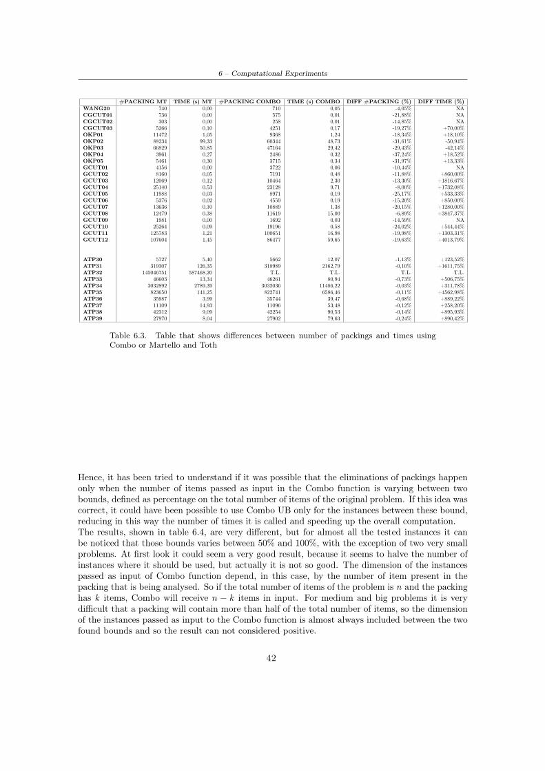
6 – Computational Experiments
#PACKING MT TIME (s) MT #PACKING COMBO TIME (s) COMBO DIFF #PACKING (%) DIFF TIME (%)WANG20 740 0,00 710 0,05 -4,05% NACGCUT01 736 0,00 575 0,01 -21,88% NACGCUT02 303 0,00 258 0,01 -14,85% NACGCUT03 5266 0,10 4251 0,17 -19,27% +70,00%OKP01 11472 1,05 9368 1,24 -18,34% +18,10%OKP02 88234 99,33 60344 48,73 -31,61% -50,94%OKP03 66829 50,85 47164 29,42 -29,43% -42,14%OKP04 3961 0,27 2486 0,32 -37,24% +18,52%OKP05 5461 0,30 3715 0,34 -31,97% +13,33%GCUT01 4156 0,00 3722 0,06 -10,44% NAGCUT02 8160 0,05 7191 0,48 -11,88% +860,00%GCUT03 12069 0,12 10464 2,30 -13,30% +1816,67%GCUT04 25140 0,53 23128 9,71 -8,00% +1732,08%GCUT05 11988 0,03 8971 0,19 -25,17% +533,33%GCUT06 5376 0,02 4559 0,19 -15,20% +850,00%GCUT07 13636 0,10 10889 1,38 -20,15% +1280,00%GCUT08 12479 0,38 11619 15,00 -6,89% +3847,37%GCUT09 1981 0,00 1692 0,03 -14,59% NAGCUT10 25264 0,09 19196 0,58 -24,02% +544,44%GCUT11 125783 1,21 100651 16,98 -19,98% +1303,31%GCUT12 107604 1,45 86477 59,65 -19,63% +4013,79%
ATP30 5727 5,40 5662 12,07 -1,13% +123,52%ATP31 319307 126,35 318989 2162,79 -0,10% +1611,75%ATP32 145046751 587468,20 T.L. T.L. T.L. T.L.ATP33 46603 13,34 46261 80,94 -0,73% +506,75%ATP34 3032892 2789,39 3032036 11486,22 -0,03% +311,78%ATP35 823650 141,25 822741 6586,46 -0,11% +4562,98%ATP36 35987 3,99 35744 39,47 -0,68% +889,22%ATP37 11109 14,93 11096 53,48 -0,12% +258,20%ATP38 42312 9,09 42254 90,53 -0,14% +895,93%ATP39 27970 8,04 27902 79,63 -0,24% +890,42%
Table 6.3. Table that shows differences between number of packings and times usingCombo or Martello and Toth
Hence, it has been tried to understand if it was possible that the eliminations of packings happenonly when the number of items passed as input in the Combo function is varying between twobounds, defined as percentage on the total number of items of the original problem. If this idea wascorrect, it could have been possible to use Combo UB only for the instances between these bound,reducing in this way the number of times it is called and speeding up the overall computation.The results, shown in table 6.4, are very different, but for almost all the tested instances it canbe noticed that those bounds varies between 50% and 100%, with the exception of two very smallproblems. At first look it could seem a very good result, because it seems to halve the number ofinstances where it should be used, but actually it is not so good. The dimension of the instancespassed as input of Combo function depend, in this case, by the number of item present in thepacking that is being analysed. So if the total number of items of the problem is n and the packinghas k items, Combo will receive n − k items in input. For medium and big problems it is verydifficult that a packing will contain more than half of the total number of items, so the dimensionof the instances passed as input to the Combo function is almost always included between the twofound bounds and so the result can not considered positive.
42

6 – Computational Experiments
Dim Initial KP n_max(1) n_min (2) % on the total (1) % on the total (2)WANG20 42 39 33 92,86% 78,57%CGCUT01 16 15 6 93,75% 37,50%CGCUT02 23 22 10 95,65% 43,48%CGCUT03 62 61 53 98,39% 85,48%OKP01 50 49 33 98,00% 66,00%OKP02 30 29 19 96,67% 63,33%OKP03 30 29 19 96,67% 63,33%OKP04 61 60 50 98,36% 81,97%OKP05 97 96 84 98,97% 86,60%GCUT01 10 9 6 90,00% 60,00%GCUT02 20 19 14 95,00% 70,00%GCUT03 30 29 23 96,67% 76,67%GCUT04 50 48 42 96,00% 84,00%GCUT05 10 9 5 90,00% 50,00%GCUT06 20 19 15 95,00% 75,00%GCUT07 30 29 25 96,67% 83,33%GCUT08 50 48 43 96,00% 86,00%GCUT09 10 9 5 90,00% 50,00%GCUT10 20 19 15 95,00% 75,00%GCUT11 30 29 23 96,67% 76,67%GCUT12 50 49 44 98,00% 88,00%
ATP30 192 164 145 85,42% 75,52%ATP31 258 241 208 93,41% 80,62%ATP32 249 T.L. T.L. T.L. T.L.ATP33 224 213 184 95,09% 82,14%ATP34 130 110 66 84,62% 50,77%ATP35 153 135 107 88,24% 69,93%ATP36 153 137 115 89,54% 75,16%ATP37 222 208 186 93,69% 83,78%ATP38 202 182 157 90,10% 77,72%ATP39 163 150 133 92,02% 81,60%
Table 6.4. Table that shows maximal and minimal percentage of the total elements for which usingCombo at least one packing is cut
6.4 Performance of G2KP
First of all the dimension of loops in heuristicG2KP has been defined. For the inner loop has beenseen empirically that it is better to avoid to perform it too many times, because if a very goodheuristic solution is found early in the execution, it is very difficult to find values that are betterand that at the same time are also coming from a set of possibly feasible items. So it has beendecided to set the variable NUMBER_OF_INNER_LOOPS to the value 50. On the other hand,for the outer cycle, it has been necessary to execute it a sufficient number of times to increase thepossibility of finding a good heuristic solution, to decrease the chances of being obliged to performthe procedure recursive with a too small lower bound, as described before. So it has been decidedafter some tests, that a good compromise between execution speed and goodness of the solution isto set the variable NUMBER_OF_LOOPS to the value 2000000.
Let us now discuss about the performance of the algorithm for G2KP.Normally, we should describe performances of the entire algorithm exactG2KP. But, as these
43

6 – Computational Experiments
performances can vary a lot depending on the result of the heuristic algorithm, which is very ran-domized, we have decided to focus here more on performances of the procedure recursive, which isthe real bottleneck of the algorithm and that is not affected by random values. The computationof procedure recursive has been performed with the optimal lower bound passed as input of thefunction to determine computational time and maximum memory needed for the execution of thisfunction. The values computed for exactG2KP must be considered only as indicative because ofthe already mentioned random component.Tests have been executed on a blade server used for cluster computing. On the cluster any 32- or64-bit application can be run that might normally be run on a linux pc or any program that hasbeen recompiled. The cluster is composed by 14 computing resources, each one with:
• 2 quad core processors Intel Xeon E5450 (12M Cache, 3.00 GHz, 1333 MHz FSB);
• 16 GB RAM;
• 2 hard disk of 72 GB in configuration RAID-1 (mirror).
The various requests are managed by the server management program, queued according to a pri-ority system and executed by the most appropriate computing resource at that time. The resultsof computation that normally would appear on the screen are saved in an output file. The man-agement program adopted is Sun Grid Engine (SGE). To launch a program is necessary to createa job file containing the required computing resources, the program to run, the files to use as inputand the file where to write as output. This job can be then used to queue the request.With SGE on the cluster different groups have been defined, each one with more or less privileges.We belonged to the group called "Medium" so the maximum available memory (i.e. memory limitM.L.) for our test was 10 GB. The maximal computational time (i.e. time limit T.L.) has beenassumed to be 15 days.
In the following table (Table 6.5), the obtained results are presented.
44

6 – Computational Experiments
#SHAPES #ITEMS OPT SOL TIME RECURS (s) MEMORY RECURS (MB) TIME EXACT (s) MEMORY EXACT (MB)WANG20 19 42 2721 0,00 NA 10,01 125,879CGCUT01 7 16 244 0,00 NA 7,46 125,879CGCUT02 10 23 2892 0,00 NA 4,66 125,879CGCUT03 19 62 1860 0,08 NA 311,88 125,879OKP01 15 50 27589 0,91 126,383 36,62 126,508OKP02 30 30 22502 64,48 132,988 3161,06 133,652OKP03 30 30 24019 23,73 132,945 1240,51 133,621OKP04 33 61 32893 0,21 NA 306,78 126,164OKP05 29 97 27923 0,23 NA 42,88 126,160GCUT01 10 10 48368 0,00 NA 8,02 125,875GCUT02 20 20 59307 0,04 NA 14,74 126,152GCUT03 30 30 60241 0,10 NA 10,61 126,754GCUT04 50 50 60942 0,40 NA 32,09 127,738GCUT05 10 10 195582 0,03 NA 6,59 126,375GCUT06 20 20 236305 0,01 NA 12,04 125,887GCUT07 30 30 238974 0,08 NA 21,71 126,973GCUT08 50 50 245758 0,20 NA 26,24 127,668GCUT09 10 10 919476 0,00 NA 4,75 125,879GCUT10 20 20 903435 0,07 NA 13,46 126,918GCUT11 30 30 955389 0,66 134,848 30,13 135,549GCUT12 50 50 970744 0,79 NA 60,38 137,758GCUT13 32 32 8532720 T.L. - T.L. -
ATP30 38 192 140904 2,77 127,633 45,75 127,777ATP31 51 258 823976 48,52 162,066 68927,06 2503,000ATP32 55 249 38068 587468,20 9189,000 587513,00 9189,000ATP33 44 224 236611 7,27 131,918 309,26 142,836ATP34 27 130 361398 1645,50 328,297 79863,59 NAATP35 29 153 621021 81,34 186,473 6241,58 371,211ATP36 28 153 130744 2,22 128,570 108,17 135,051ATP37 43 222 387276 12,69 131,137 551,75 146,109ATP38 40 202 261395 5,92 131,746 369,20 179,875ATP39 33 163 268750 5,00 134,766 219,81 138,270
ATP40 56 290 67154 255923,83 1071,000 T.L. -ATP41 36 177 206542 T.L. - T.L. -ATP42 59 325 33503 T.L. - T.L. -ATP43 49 259 214651 T.L. - T.L. -ATP44 39 196 73868 T.L. - T.L. -ATP45 33 156 74691 T.L. - T.L. -ATP46 42 197 149911 23949,42 464,301 T.L. -ATP47 43 204 150234 T.L. - T.L. -ATP48 34 167 167660 T.L. - T.L. -ATP49 25 119 219354 T.L. - T.L. -
Table 6.5. Table that shows performances of procedure Recursive and of exactG2KP
From the table it is possible to see that for the greater part of the input instances has been possibleto find a solution. For those for that it has not been possible because of the time limit, during theirexecution we were checking the maximum memory usage and it was quite low (few gigabytes), sowe can say that probably with no limitations of time they would have terminated. But anyway, wehave must remember that this is not the whole algorithm to compute G2KP, but just the recursivepart, which is repeated many times. So it will be important in a possible future work trying tospeed up the algorithm to be able to end up also all the ATP input files in reasonable times. Thecomputed times, anyway, must be considered as indicative, because they depend on the load of themachine.
Table 6.6 contains the values obtained by the heuristic algorithm executing it five times, so theseed that generates random values changes and different values are obtained. It also contains theaverage of these values and the optimal solution. In the last column is present which percentage ofthe optimal value is the average of the values found. This gives us a performance indicator of thealgorithm used and, because all the average values are above 70% of the optimal value and almostall also above 80%, we can say that the heuristic algorithm implemented can be considered verygood.
45

6 – Computational Experiments
OPT SOL TEST #1 TEST #2 TEST #3 TEST #4 TEST #5 AVERAGE % OF THE OPTWANG20 2721 2479 2559 2702 2307 2613 2532 93,05%CGCUT01 244 230 244 244 229 240 237 97,30%CGCUT02 2892 2360 2323 2614 2324 2343 2393 82,74%CGCUT03 1860 1600 1580 1660 1600 1560 1600 86,02%OKP01 27589 21471 21628 20906 23853 20967 21765 78,89%OKP02 22502 15744 15988 15597 16502 17591 16284 72,37%OKP03 24019 18871 18773 22130 19781 19957 19902 82,86%OKP04 32893 26214 24867 26474 26391 27360 26261 79,84%OKP05 27923 20155 21864 23321 23997 25417 22951 82,19%GCUT01 48368 48368 42025 41378 42348 48368 44497 92,00%GCUT02 59307 48288 48664 52148 55111 53323 51507 86,85%GCUT03 60241 57462 55424 58396 58714 55804 57160 94,89%GCUT04 60942 57822 60522 60195 59117 60073 59546 97,71%GCUT05 195582 177617 192907 187987 192907 189856 188255 96,25%GCUT06 236305 228442 216644 228675 216481 224166 222882 94,32%GCUT07 238974 226069 221511 232723 228130 223253 226337 94,71%GCUT08 245758 220262 232064 225736 233058 233963 229017 93,19%GCUT09 919476 786653 858697 851794 835406 851794 836869 91,02%GCUT10 903435 839394 877079 805607 827223 847308 839322 92,90%GCUT11 955389 903187 918825 864879 879182 897941 892803 93,45%GCUT12 970744 914253 941884 943625 933988 970744 940899 96,93%GCUT13 8532720 7594031 7740992 7354480 7408240 7514303 7522409 88,16%
ATP30 140904 128918 126349 126992 125459 129960 127536 90,51%ATP31 823976 761800 744577 748714 747602 759090 752357 91,31%ATP32 38068 34395 34736 34608 34795 33910 34489 90,60%ATP33 236611 212807 212897 211738 215630 209572 212529 89,82%ATP34 361398 325023 327239 329322 328881 326658 327425 90,60%ATP35 621021 562979 554089 545209 562001 573636 559583 90,11%ATP36 130744 115754 119316 117264 116164 119913 117682 90,01%ATP37 387276 342280 343677 348652 339340 343596 343509 88,70%ATP38 261395 234816 235670 236071 234105 236440 235420 90,06%ATP39 268750 247479 246807 255880 246119 248941 249045 92,67%
ATP40 67154 53495 50839 56444 52615 55423 53763 80,06%ATP41 206542 172873 180189 181823 175524 175617 177205 85,80%ATP42 33503 27062 26880 27356 26992 28645 27387 81,74%ATP43 214651 177980 167411 167800 169983 167415 170118 79,25%ATP44 73868 61166 64091 58657 58136 61032 60616 82,06%ATP45 74691 65784 66431 65358 65137 65350 65612 87,84%ATP46 149911 123669 126195 124818 127287 126526 125699 83,85%ATP47 150234 123171 123809 122932 121504 124345 123152 81,97%ATP48 167660 133433 139095 132705 138814 135845 135978 81,10%ATP49 219354 176047 169359 170733 172859 170209 171841 78,34%
Table 6.6. Table that shows average values found by the heuristic algorithm for G2KP
6.5 Performance of G2BPP
Like the case of G2KP, also for G2BPP first of all the dimension of the loop in heuristicG2BPPhas been defined. The problem here is different for two reasons: the first one is that here it ispossible to exit the loop before its end and the second one is that this loop is performed manytimes during the execution of the algorithm, not just one time at the beginning like G2KP.Starting from these considerations the value searched should not have been a too high value, butalso it was not necessary that it was too small. Eventually, after some tests, it has been seen thata good value for this variable NUMBER_OF_LOOPS is 1000.
To test the efficiency of the algorithm that solves G2BPP the same machine used for G2KPhas been adopted. Considering the performance of G2BPP in terms of computational time andmemory used, the result that we have obtained can be considered very good. For this kind of
46

6 – Computational Experiments
problem the input instances ATPs have not been considered, because we have based on the samekind of instances used by Martello and Vigo in [10]. Moreover, with this algorithm, we also wantto find the coordinates that will have the items in the packings and not only the number of binsused to pack all of them. In table 6.7 the time needed and the memory used by the instances arerepresented.
#ITEMS OPT SOL TIME (s) MEMORY (MB) 2BPP TIME (s)WANG20 42 11 0,27 NA NACGCUT01 16 2 0,02 NA 0,01CGCUT02 23 2 17,75 128,633 0,01CGCUT03 62 23 0,61 NA 0,04OKP01 50 4 16,80 126,492 NAOKP02 30 4 0,61 NA NAOKP03 30 4 385,41 126,715 NAOKP04 61 7 359,86 126,613 NAOKP05 97 - T.L. - NAGCUT01 10 5 0,02 NA 0,02GCUT02 20 6 0,14 NA 0,02GCUT03 30 8 0,10 NA 0,01GCUT04 50 14 3,67 125,875 3,73GCUT05 10 3 0,01 NA 0,01GCUT06 20 7 1,91 125,875 0,90GCUT07 30 11 0,17 NA 0,28GCUT08 50 - T.L. - T.L.GCUT09 10 3 0,01 NA 0,02GCUT10 20 8 3,73 125,875 1,22GCUT11 30 9 1264,46 125,875 909,70GCUT12 50 16 0,52 125,875 0,17GCUT13 32 2 34,09 * 0,01
Table 6.7. Table that shows performances of exactG2BPP
Comparing results with results of Martello and Vigo present in the last column, it is possible tosee that even with the addition of Guillotine constraints the optimal solution remains the samefor all instances with the exception of GCUT10. Moreover, also computational times are all veryclose to those presented in the paper and sometimes even better. The only two instances that hasa big performances decay are CGCUT02 that passes from 0.01 seconds needed for the 2BPP tothe 17.75 seconds needed here for G2BPP and GCUT13 that passes from 0.17 to 34.09. GCUT13has a * on the memory column because that is the time needed to compute only the best solution,to compute also the optimal packing much more time is needed.OKPs and WANG20 were not used by Martello and Vigo for their tests, but they have been usedhere because their size is similar to the other used instances. OKP05 is the only of these instancesthat reaches time limit, but it is not surprising because its size is almost two times bigger than allthe other considered instances.Considering the memory usage, on the other hand, results obtained are great, because the memoryused is very limited, so no problem connected with a big memory usage should be present.
47

Chapter 7
Conclusions
To conclude, therefore, a function that computes an exact packing of a Guillotine Two-dimensionalKnapsack Problem with a minimum profit z0 has been implemented. This function is also ableto return the correct position where the various items that are in the solution should have in thecontainer to obtain the correct packing.Thanks to this function it has been possible to compute first of all the exact solution for a G2KPeven without knowing a lower bound and secondly also the exact solution for a G2BPP, returningfor each item the bin where it should be packed and the correct coordinates into that bin.Moreover, to obtain these results, also two heuristic algorithms have been developed and imple-mented to speed up the global computation.
Considering the memory performances, that was the main goal, the created algorithms can be con-sidered very positively, because even with big input instances it never reaches the memory limit.Considering, on the other hand, the time performances, the procedure recursive should be im-proved, because to be able to guarantee the absence of memory problems, the speed of the algo-rithm has been sacrificed and so for many of the ATP4x instances (which are very difficult) thealgorithm is not able to end up before the time limit. Anyway this has not been a problem forG2BPP, because the instances where it is computed are not very big, because all items must bepacked, and so the procedure recursive works well, in line with the times obtained by the exactalgorithm for 2BPP implemented by Martello and Vigo.
48


Bibliography
[1] Nicos Christofides, Charles Whitlock, An algorithm for two-dimensional cutting problems.Operations Research, 1977.
[2] George B. Dantzig, Discrete Variable Extremum Problems. Operations Research 5, 1957.
[3] Mohammad Dolatabadi, Andrea Lodi, Michele Monaci, Exact algorithms for the two-dimensional guillotine knapsack. Computers & Operations Research, 2012.
[4] Matteo Fischetti, Lezioni di Ricerca Operativa. Libreria Progetto, 1995.
[5] Brian W. Kernighan, Dennis Ritchie, The C programming language. Prentice Hall, 1988.
[6] Andrea Lodi, Michele Monaci, Integer linear programming models for 2-staged two-dimensional Knapsack problems. Mathematical Programming, 2003.
[7] Silvano Martello, David Pisinger, Paolo Toth, Dynamic programming and strong bounds forthe 0-1 knapsack problem. Management Science 45, 1999.
[8] Silvano Martello, David Pisinger, Daniele Vigo, An algorithm for the three-dimensional binpacking problem. Operations Research 48, 2000.
[9] Silvano Martello, Paolo Toth, Knapsack problems: algorithms and computer implementations.Cichester: John Wiley & Sons, 1990.
[10] Silvano Martello, Daniele Vigo Exact Solution of the Two-Dimensional Finite Bin PackingProblem. Management Science 44, 1988.
[11] Michele Monaci, Algoritmi Euristici. Dipartimento di Ingegneria dell’Informazione, Universitàdi Padova, 2012.
[12] Gerhard J. Woeginger, Exact algorithms for NP-Hard problems: a survey. Combinatorialoptimization - Eureka, you shrink! 2003.
[13] http://www.eclipse.org.
[14] http://www.gnuplot.info
50

Bibliography
[15] http://www.diku.dk/∼pisinger
[16] http://valgrind.org
51


Acknowledgements
Ringrazio innanzitutto il professor Michele Monaci per avermi dato l’opportunità di cimentarmiin questa tesi di laurea e per essere sempre stato super disponibile e rapido nel chiarire i dubbi chemi si presentavano.
Ringrazio i miei genitori per essermi stati sempre accanto, per aver creduto in me anche diquanto lo facessi io e per aver "tirà fora i schei" per tutti questi anni.
Ringrazio mio fratello Michele che per tanti anni è servito come valvola di sfogo per avermisopportato.
Ringrazio Federica per essermi stata la persona più vicina in questi ultimi mesi e avermi sempreincoraggiato e sostenuto anche nei momenti peggiori.
Ringrazio tutti i miei amici dell’università, Alby, Alvi, Bedo, Dani, Ele, Fede, Fra, Gian,Giulio, Glo, Luci, Marco, Marty, Peli, Pol, Ross, Seba. Sono riusciti a rendermi menopesanti questi anni di università e per molti aspetti, penso, anche una persona migliore. Senza divoi non ce l’avrei mai fatta. Grazie, davvero.
Ringrazio i miei compagni di viaggio nella piovosa terra Scozzese Andrea, Antonio e Luca, peraver condiviso così tanto con me ed essere stati la mia "famiglia" per 5 mesi. Ringrazio ancheDaniele e Diane che a Glasgow ci hanno fatto sentire come a casa.
Ringrazio i miei compagni di basket, l’ammiraglio Faffi, Livio, Malox e Scotti per i campi-onati e i tornei vinti in questi anni. Senza dimenticare i litri di birra bevuti.
Ringrazio tutti gli altri amici che, anche se non riusciamo a vederci quanto vorrei, so che mivogliono bene e che potrò sempre contare su di loro.
53