Approximation Algorithms for

2-Dimensional Packing Problems

Klaus Jansen

Universitat Kiel

1

Overview

• Introduction

• Algorithms NFDH, FFDH

• Algorithm by Kenyon, Remila

• Algorithm by Jansen, Solis-Oba

• Open problems

2

2D packing problem

Given:

• n rectangles Rj = (wj, hj) of width wj ≤ 1 and height hj ≤ 1,

• a strip of width 1 and unbounded height.

Problem: pack the n rectangles into the strip (without overlap and

rotation) while minimizing the total height used.

Complexity: NP-hard (contains bin packing as special case).

3

Example

R1

R2

R3 R6

R4

R5

1

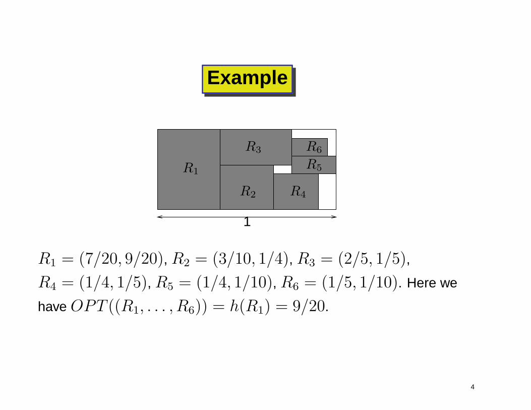
R1 = (7/20, 9/20), R2 = (3/10, 1/4), R3 = (2/5, 1/5),

R4 = (1/4, 1/5), R5 = (1/4, 1/10), R6 = (1/5, 1/10). Here we

have OPT ((R1, . . . , R6)) = h(R1) = 9/20.

4

Application I

• Cutting Stock : cutting patterns of objects out of a large strip of

material (like cloth, paper or steel).

• Goal : minimize the waste of material.

5

Application II

• Scheduling : compute a schedule for a set of jobs each requiring

a certain number of resources (machines, processors or memory

locations).

• Goal : minimum length of the schedule (minimum makespan).

6

Application III

• VLSI Design : placement of modules on a chip.

• Goal : minimum area of the chip.

7

Approximation algorithms

for an optimization problem are methods which for each instance L of

the problem compute efficiently a feasible solution with provable

performance guarantee.

We compare

A(L) the height computed by algorithm A.

OPT (L) the minimum height among all solutions.

8

Absolute performance ratio

Worst Case :

For all instances L we have:

A(L) ≤ aOPT (L)

Goal : a ≥ 1 should be close to 1.

9

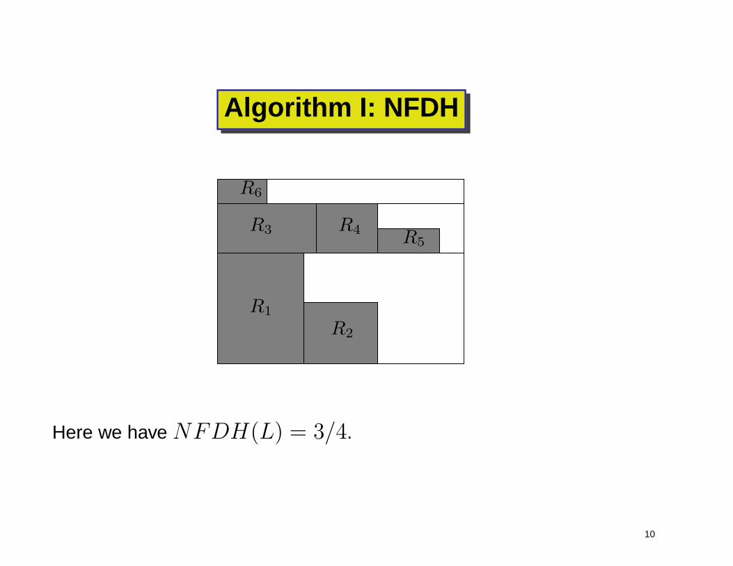
Algorithm I: NFDH

R1

R2

R3 R4R5

R6

Here we have NFDH(L) = 3/4.

10

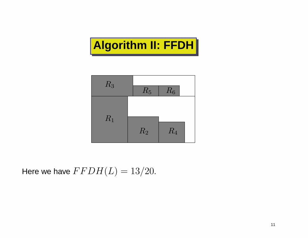
Algorithm II: FFDH

R1

R3

R4R2

R5 R6

Here we have FFDH(L) = 13/20.

11

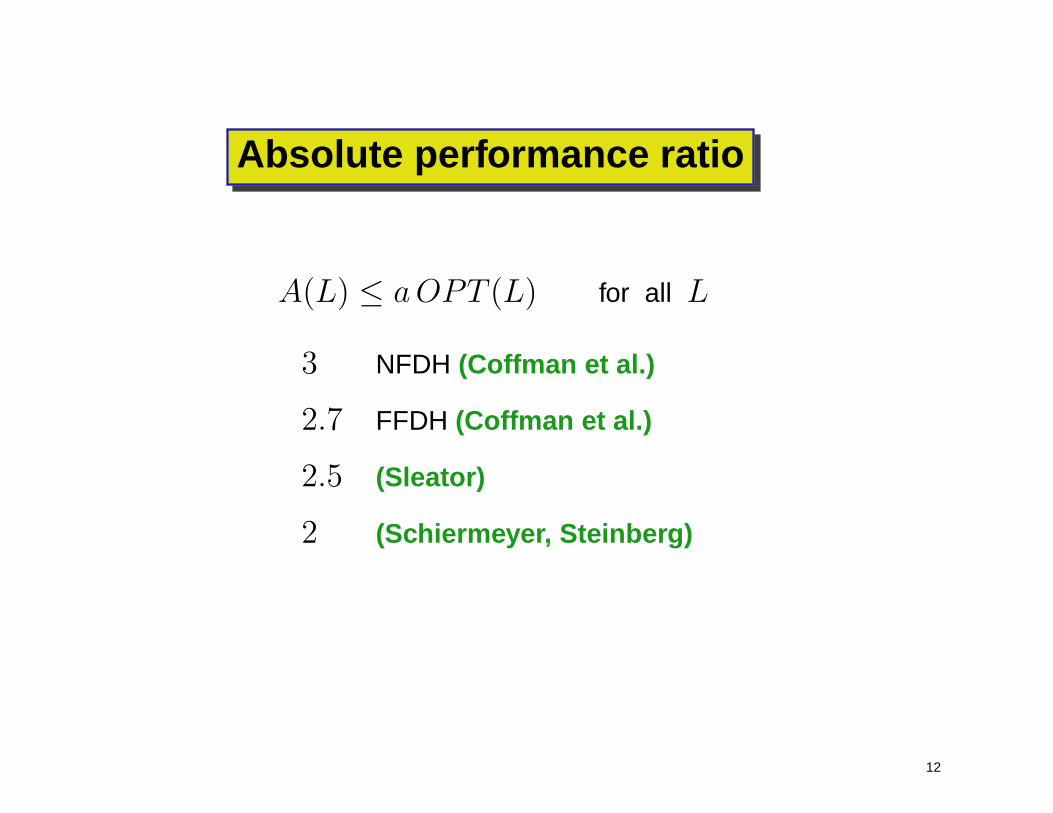
Absolute performance ratio

A(L) ≤ aOPT (L) for all L

3 NFDH (Coffman et al.)

2.7 FFDH (Coffman et al.)

2.5 (Sleator)

2 (Schiermeyer, Steinberg)

12

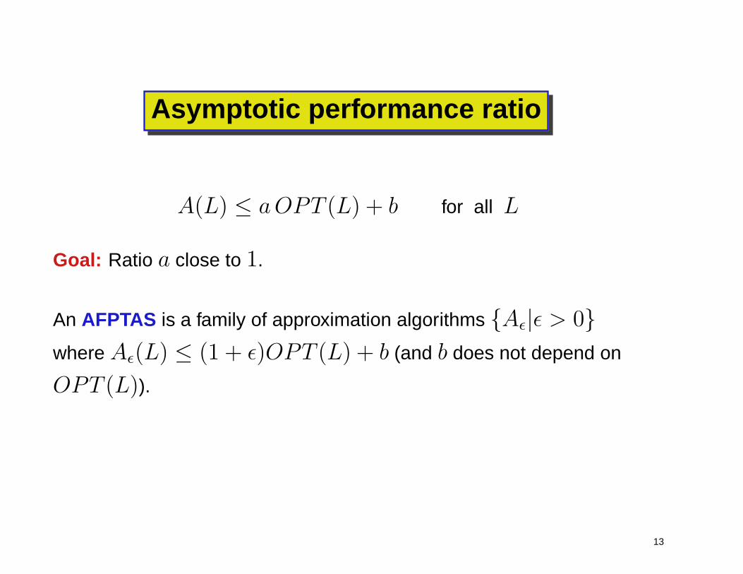
Asymptotic performance ratio

A(L) ≤ aOPT (L) + b for all L

Goal: Ratio a close to 1.

An AFPTAS is a family of approximation algorithms {Aǫ|ǫ > 0}

where Aǫ(L) ≤ (1 + ǫ)OPT (L) + b (and b does not depend on

OPT (L)).

13

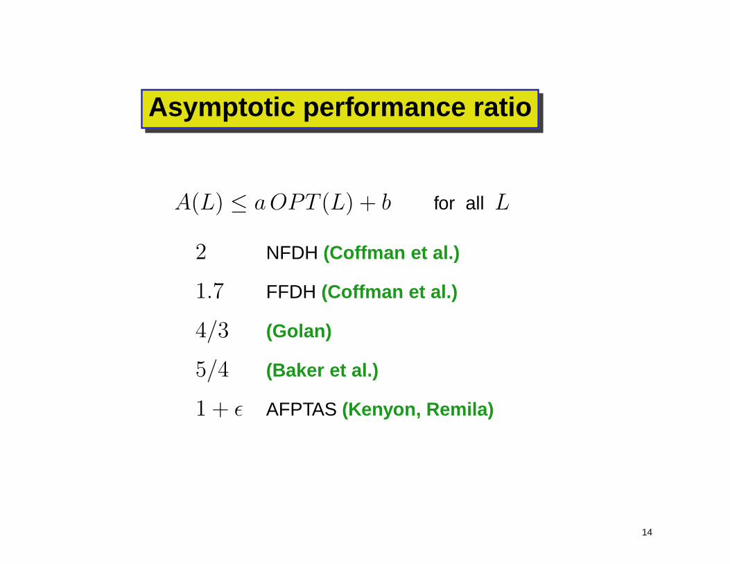
Asymptotic performance ratio

A(L) ≤ aOPT (L) + b for all L

2 NFDH (Coffman et al.)

1.7 FFDH (Coffman et al.)

4/3 (Golan)

5/4 (Baker et al.)

1 + ǫ AFPTAS (Kenyon, Remila)

14

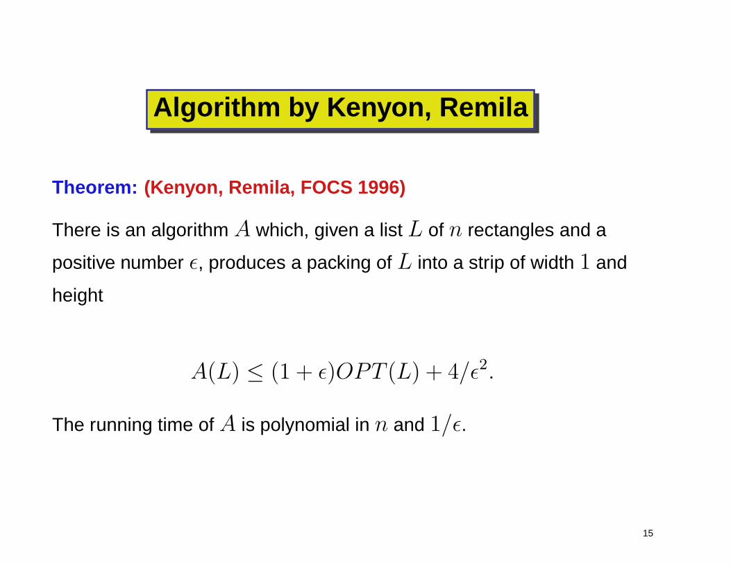
Algorithm by Kenyon, Remila

Theorem: (Kenyon, Remila, FOCS 1996)

There is an algorithm A which, given a list L of n rectangles and a

positive number ǫ, produces a packing of L into a strip of width 1 and

height

A(L) ≤ (1 + ǫ)OPT (L) + 4/ǫ2.

The running time of A is polynomial in n and 1/ǫ.

15

Main ideas of the algorithm

(a) partition the list L into narrow and wide rectangles,

(b) round the wide rectangles to obtain a constant number of widths,

(c) solve a linear program to pack the wide rectangles,

(d) use a modified version of NFDH to pack the narrow rectangles.

16

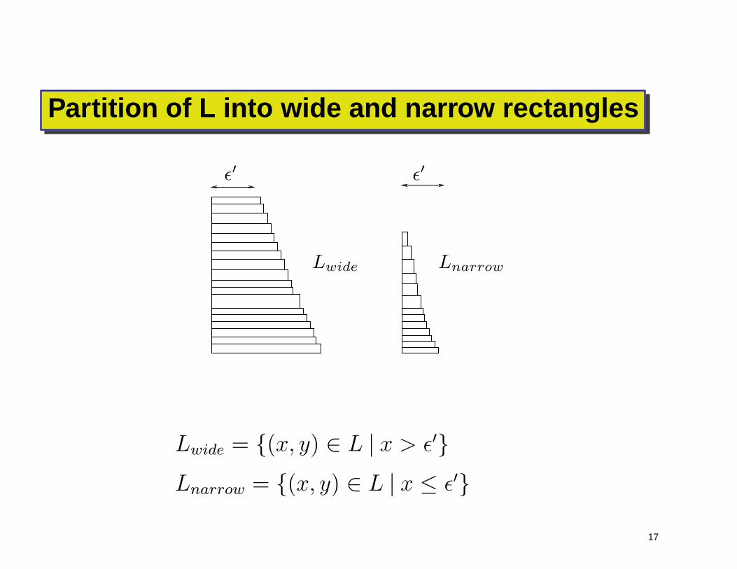
Partition of L into wide and narrow rectangles

ǫ′ ǫ′

Lwide Lnarrow

Lwide = {(x, y) ∈ L | x > ǫ′}

Lnarrow = {(x, y) ∈ L | x ≤ ǫ′}

17

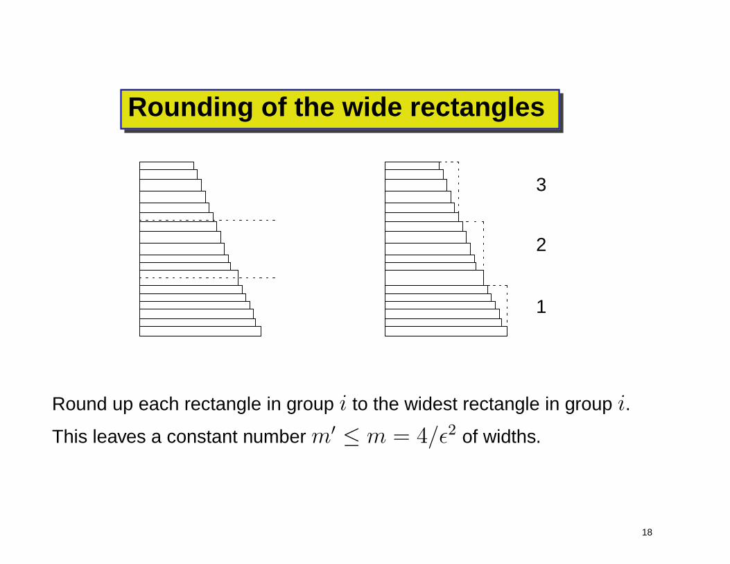
Rounding of the wide rectangles

1

2

3

Round up each rectangle in group i to the widest rectangle in group i.

This leaves a constant number m′ ≤ m = 4/ǫ2 of widths.

18

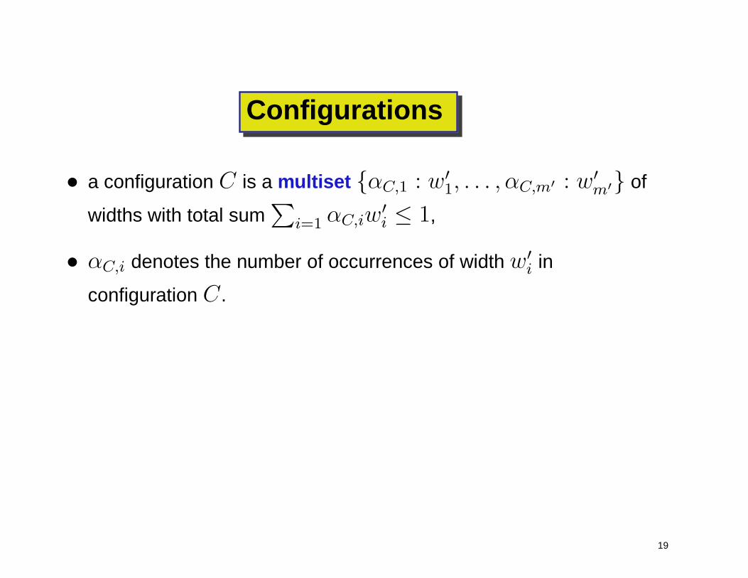
Configurations

• a configuration C is a multiset {αC,1 : w′

1, . . . , αC,m′ : w′

m′} of

widths with total sum∑

i=1αC,iw

′

i ≤ 1,

• αC,i denotes the number of occurrences of width w′

i in

configuration C .

19

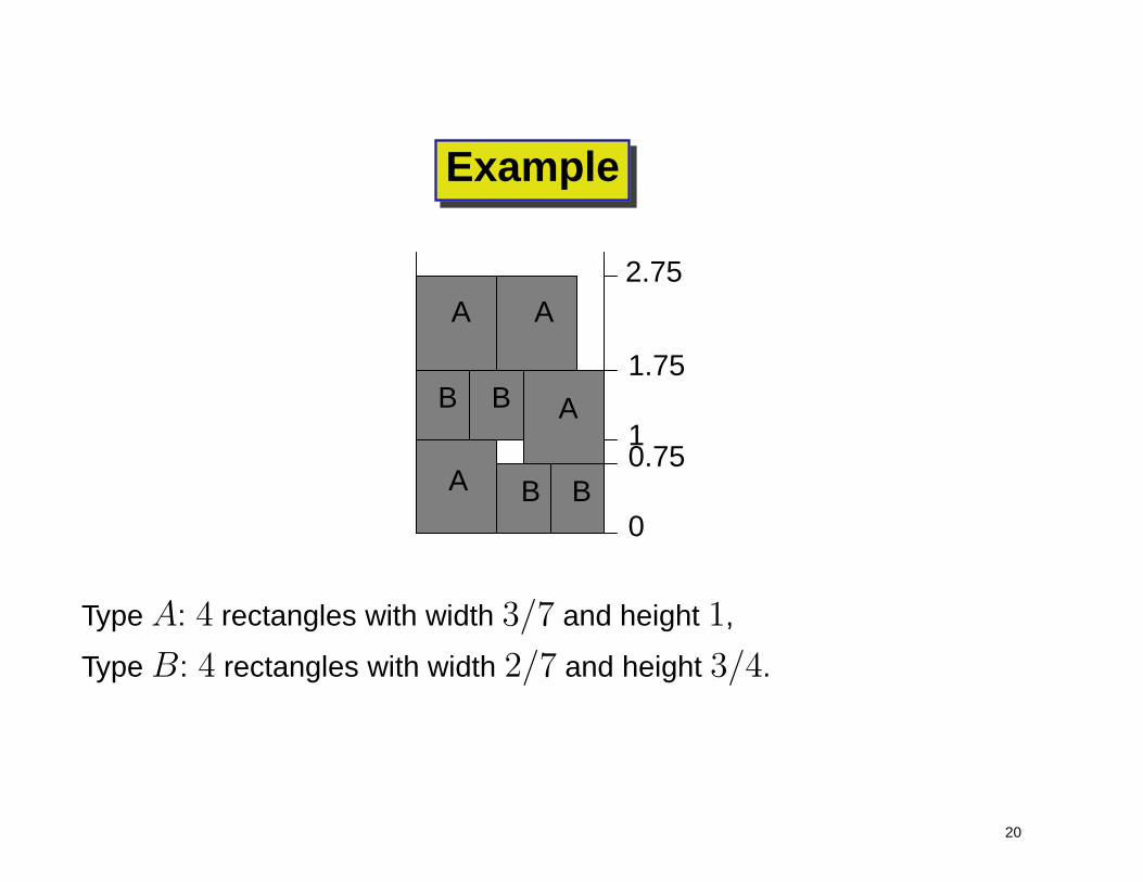
Example

0

0.751

1.75

2.75AA

B B A

A B B

Type A: 4 rectangles with width 3/7 and height 1,

Type B: 4 rectangles with width 2/7 and height 3/4.

20

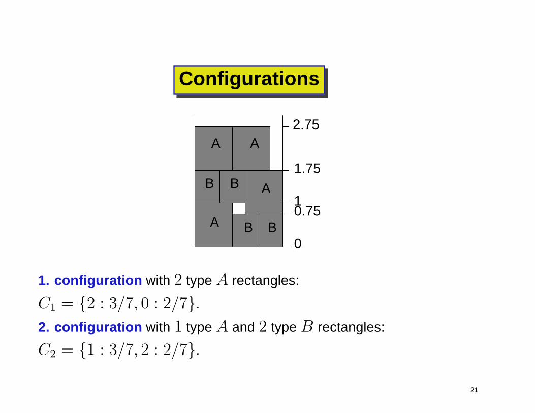
Configurations

0

0.751

1.75

2.75AA

B B A

A B B

1. configuration with 2 type A rectangles:

C1 = {2 : 3/7, 0 : 2/7}.

2. configuration with 1 type A and 2 type B rectangles:

C2 = {1 : 3/7, 2 : 2/7}.

21

Linear program

Use for each configuration C a positive variable xC ≥ 0 that

represents the total height of configuration C in the solution.

Objective function:∑

C xC is the total height of the packing.

22

Important inequality

βi the sum of the heights of all rectangles with width w′

i.

αC,i the number of occurrences of w′

i in configuration C .

Inequality:∑

C αC,ixC ≥ βi for i = 1, . . . ,m′.

Idea: The configurations must reserve enough space for the

rectangles with width w′

i.

23

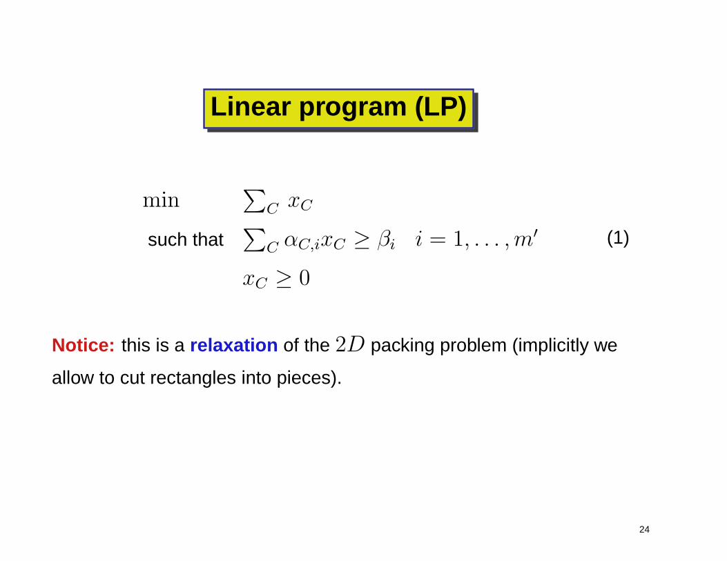
Linear program (LP)

min∑

C xC

such that∑

C αC,ixC ≥ βi i = 1, . . . ,m′

xC ≥ 0

(1)

Notice: this is a relaxation of the 2D packing problem (implicitly we

allow to cut rectangles into pieces).

24

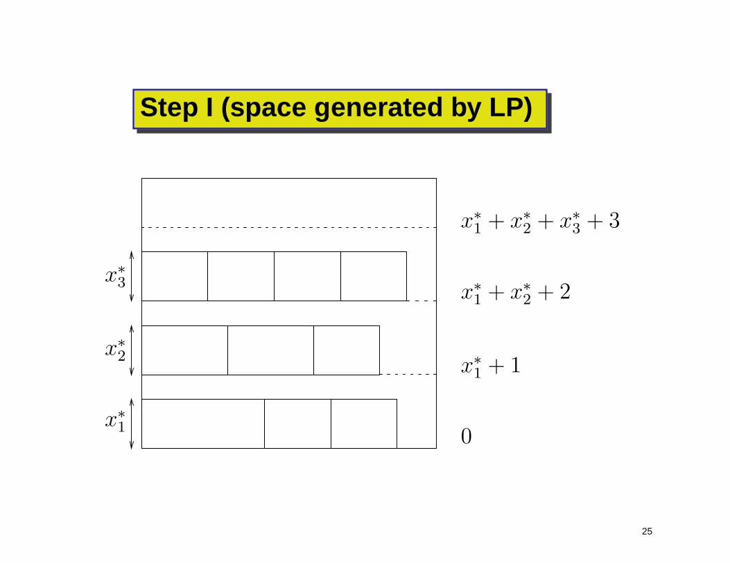
Step I (space generated by LP)

x∗

1+ x∗

2+ x∗

3+ 3

x∗

1+ x∗

2+ 2

x∗

1+ 1

0x∗

1

x∗

2

x∗

3

25

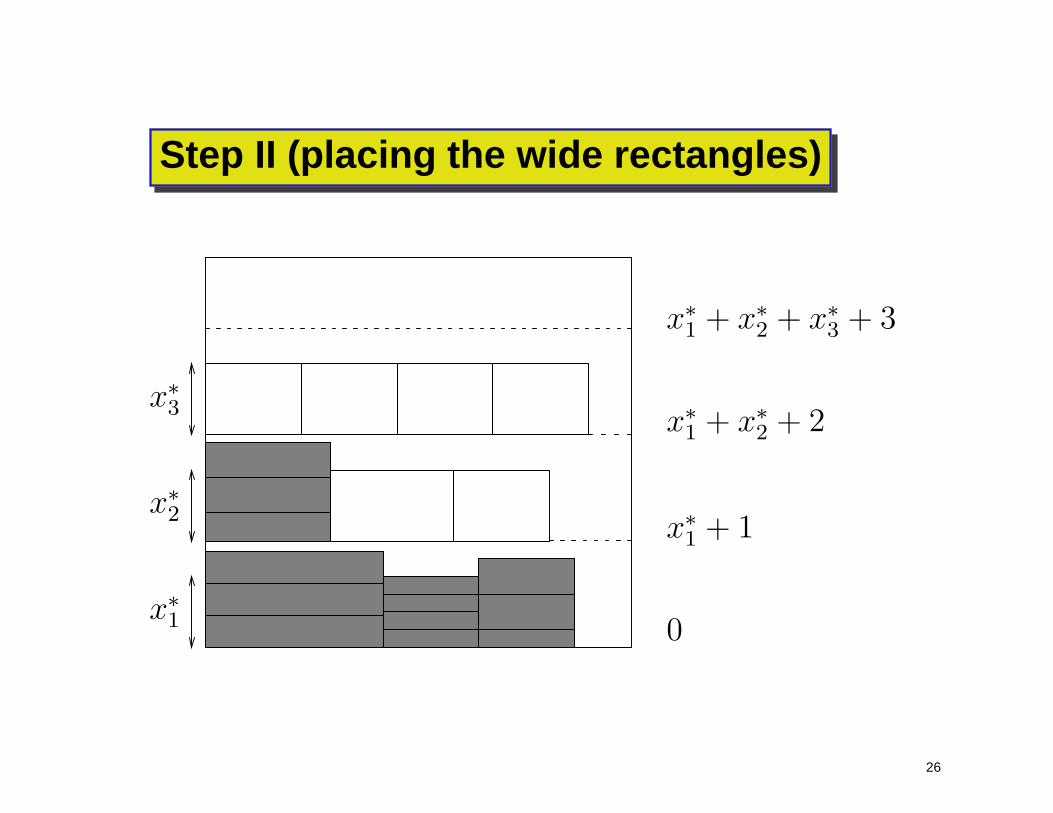
Step II (placing the wide rectangles)

x∗

1+ x∗

2+ x∗

3+ 3

x∗

1+ x∗

2+ 2

x∗

1+ 1

0x∗

1

x∗

2

x∗

3

26

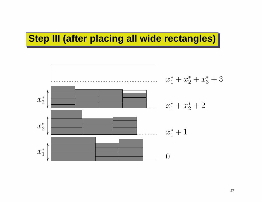
Step III (after placing all wide rectangles)

0

x∗

1+ 1

x∗

1+ x∗

2+ 2

x∗

1+ x∗

2+ x∗

3+ 3

x∗

3

x∗

2

x∗

1

27

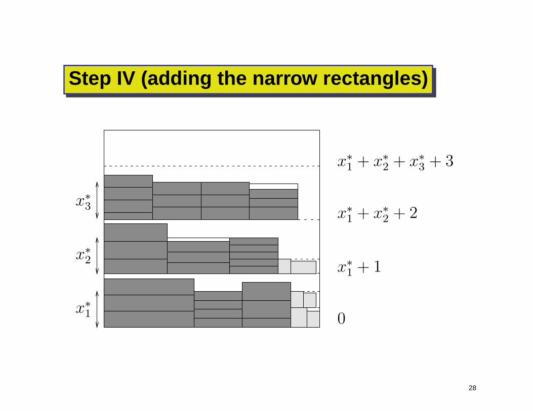
Step IV (adding the narrow rectangles)

x∗

1+ x∗

2+ x∗

3+ 3

x∗

1+ x∗

2+ 2

x∗

1+ 1

0x∗

1

x∗

2

x∗

3

28

New Result

Theorem: (Jansen, Solis-Oba 2006)

There is an approximation algorithm A, which computes a packing

into a strip of width 1 and height

A(L) ≤ (1 + ǫ)OPT (L) + 1

for any ǫ > 0.

29

2D knapsack problem

Given:

• n rectangles Ri = (wi, hi) of width wi ≤ 1, height hi ≤ 1 and

profit pi > 0.

Find: a subset R′ ⊂ {R1, . . . , Rn} which can be packed into a

square [0, 1] × [0, 1].

Goal: maximize the total profit∑

Ri∈R′ pi.

30

Example

1

1

R1R2

R3 R4

R5

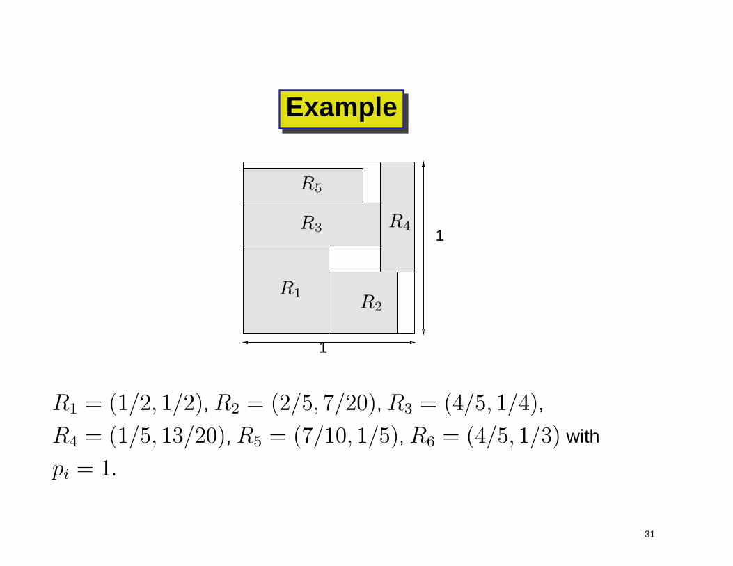
R1 = (1/2, 1/2), R2 = (2/5, 7/20), R3 = (4/5, 1/4),

R4 = (1/5, 13/20), R5 = (7/10, 1/5), R6 = (4/5, 1/3) with

pi = 1.

31

New result

Theorem: (Jansen, Solis-Oba 2006) There is an algorithm B which

finds a subset R′ ⊂ {R1, . . . , Rn} that can be packed into a

rectangle of width 1 and height 1 + ǫ and has total profit

B(L) ≥ (1 − ǫ)OPT (L),

where OPT (L) is the maximum profit among all subsets (that fit into

a square [0, 1] × [0, 1]).

32

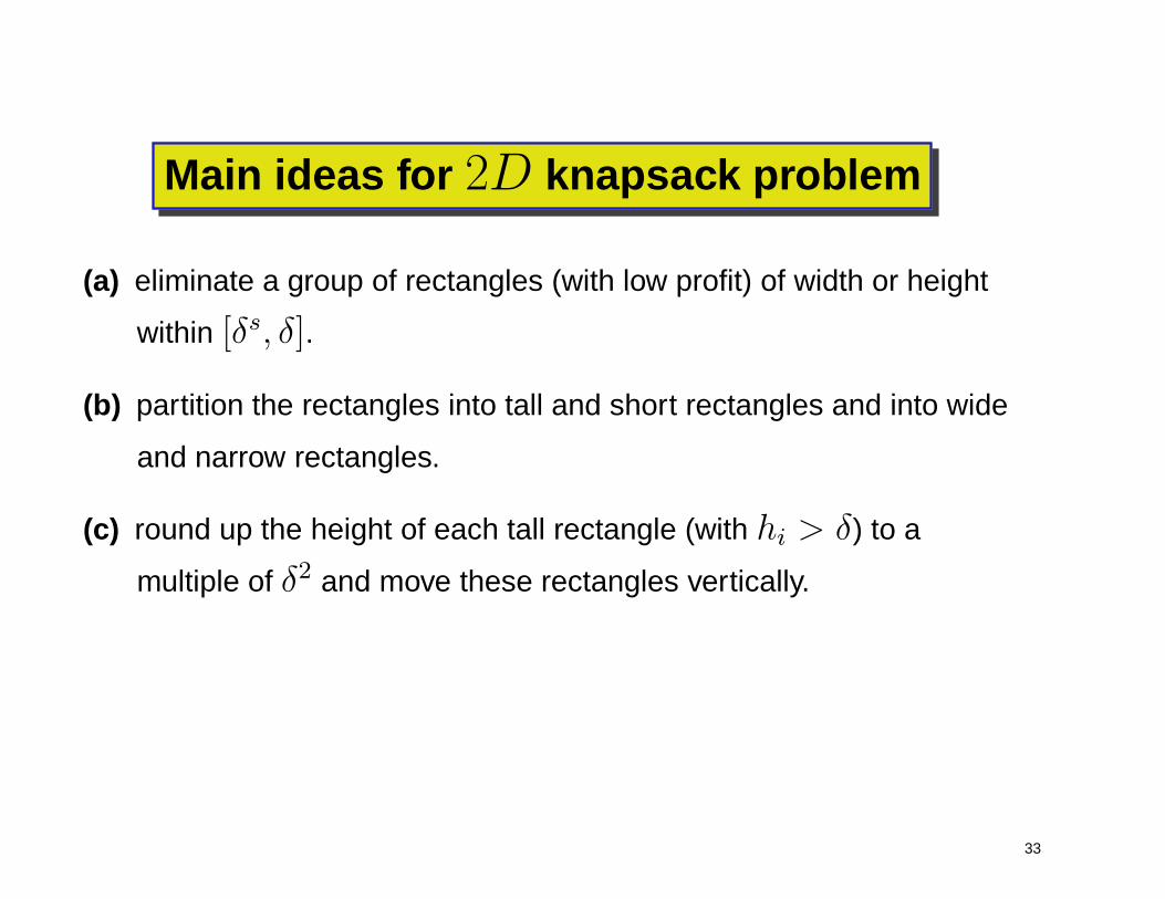
Main ideas for 2D knapsack problem

(a) eliminate a group of rectangles (with low profit) of width or height

within [δs, δ].

(b) partition the rectangles into tall and short rectangles and into wide

and narrow rectangles.

(c) round up the height of each tall rectangle (with hi > δ) to a

multiple of δ2 and move these rectangles vertically.

33

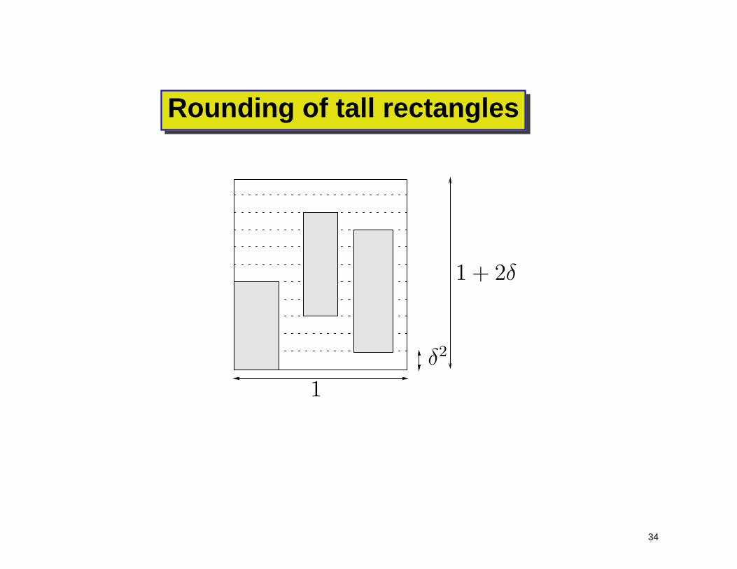
Rounding of tall rectangles

1

δ2

1 + 2δ

34

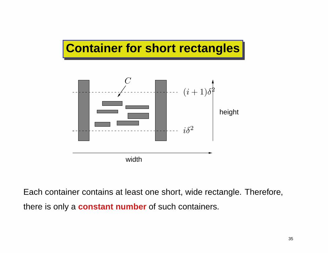
Container for short rectangles

iδ2

(i + 1)δ2

height

width

C

Each container contains at least one short, wide rectangle. Therefore,

there is only a constant number of such containers.

35

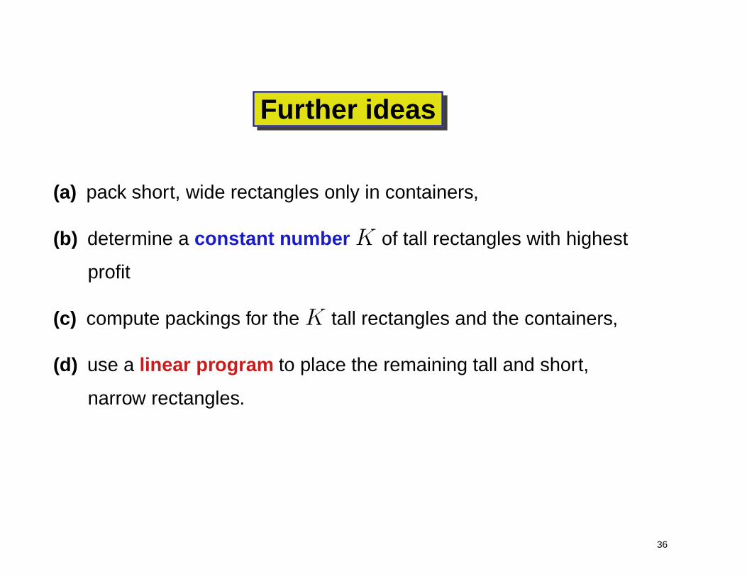
Further ideas

(a) pack short, wide rectangles only in containers,

(b) determine a constant number K of tall rectangles with highest

profit

(c) compute packings for the K tall rectangles and the containers,

(d) use a linear program to place the remaining tall and short,

narrow rectangles.

36

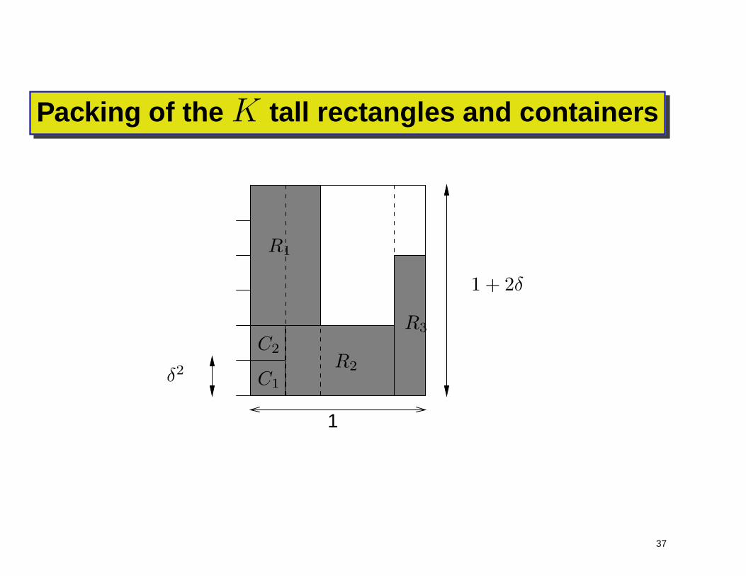
Packing of the K tall rectangles and containers

δ2

R3

C1

C2

1 + 2δ

R1

R2

1

37

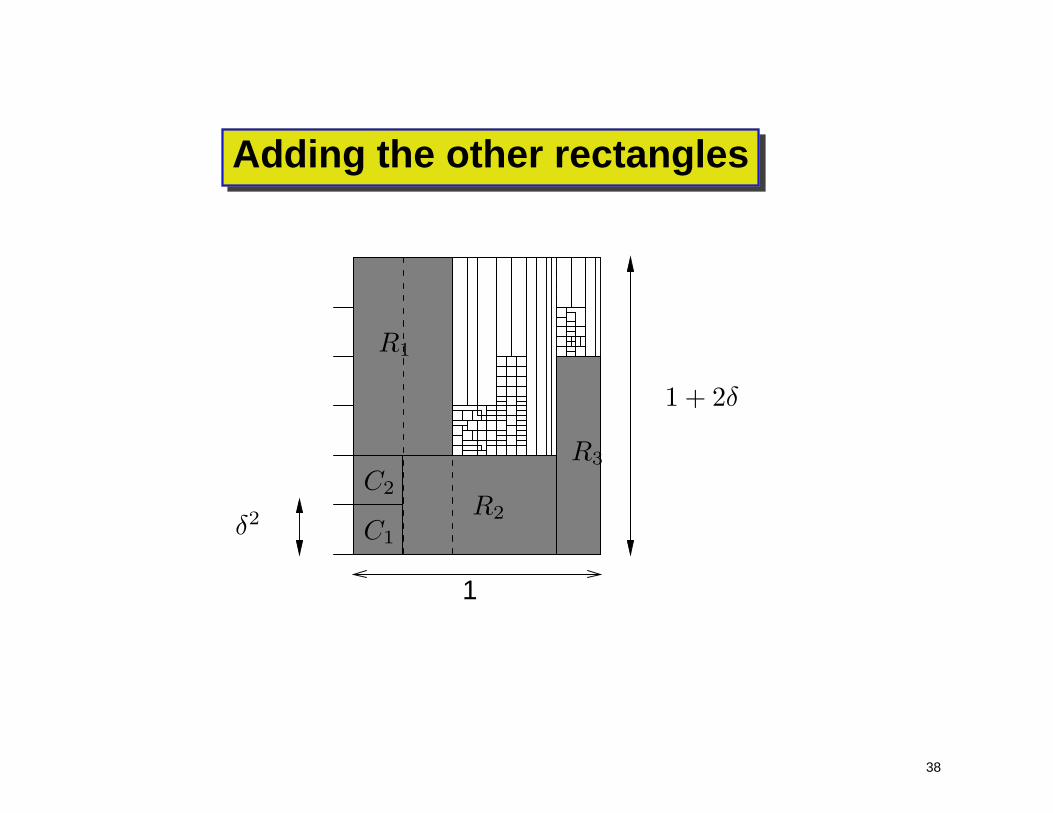
Adding the other rectangles

δ2

R3

C1

C2

1 + 2δ

R1

R2

1

38

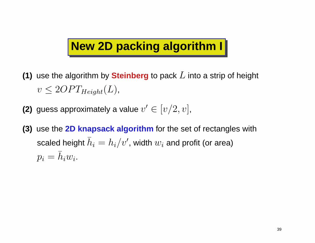
New 2D packing algorithm I

(1) use the algorithm by Steinberg to pack L into a strip of height

v ≤ 2OPTHeight(L),

(2) guess approximately a value v′ ∈ [v/2, v],

(3) use the 2D knapsack algorithm for the set of rectangles with

scaled height hi = hi/v′, width wi and profit (or area)

pi = hiwi.

39

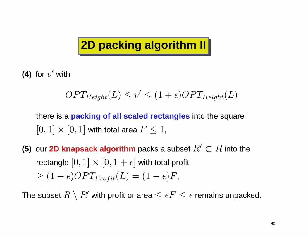
2D packing algorithm II

(4) for v′ with

OPTHeight(L) ≤ v′ ≤ (1 + ǫ)OPTHeight(L)

there is a packing of all scaled rectangles into the square

[0, 1] × [0, 1] with total area F ≤ 1,

(5) our 2D knapsack algorithm packs a subset R′ ⊂ R into the

rectangle [0, 1] × [0, 1 + ǫ] with total profit

≥ (1 − ǫ)OPTProfit(L) = (1 − ǫ)F ,

The subset R \ R′ with profit or area ≤ ǫF ≤ ǫ remains unpacked.

40

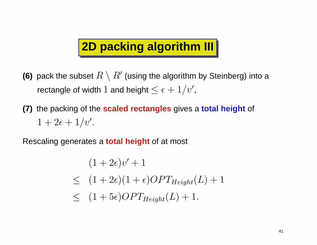
2D packing algorithm III

(6) pack the subset R \ R′ (using the algorithm by Steinberg) into a

rectangle of width 1 and height ≤ ǫ + 1/v′,

(7) the packing of the scaled rectangles gives a total height of

1 + 2ǫ + 1/v′.

Rescaling generates a total height of at most

(1 + 2ǫ)v′ + 1

≤ (1 + 2ǫ)(1 + ǫ)OPTHeight(L) + 1

≤ (1 + 5ǫ)OPTHeight(L) + 1.

41

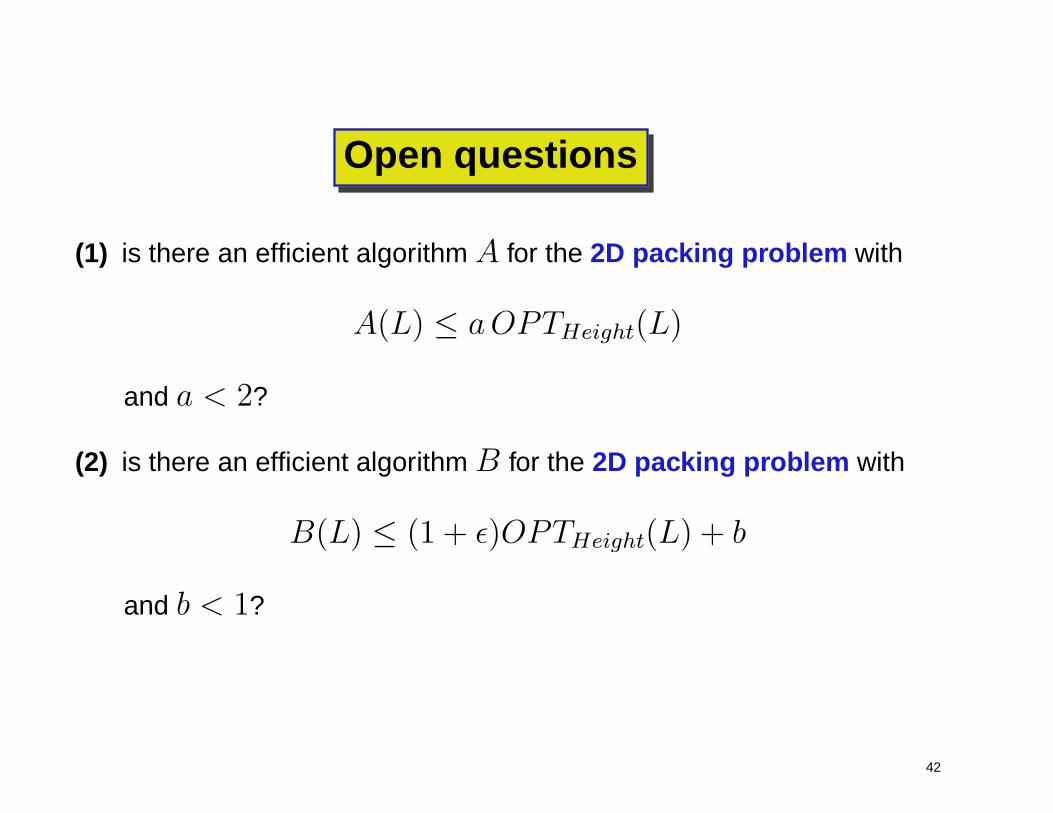
Open questions

(1) is there an efficient algorithm A for the 2D packing problem with

A(L) ≤ aOPTHeight(L)

and a < 2?

(2) is there an efficient algorithm B for the 2D packing problem with

B(L) ≤ (1 + ǫ)OPTHeight(L) + b

and b < 1?

42