Exact Algorithms for the 2-Dimensional Strip Packing Problem

with and without Rotations

1 Mitsutoshi KENMOCHI, 2 Takashi IMAMICHI, 3 Koji NONOBE,4 Mutsunori YAGIURA, 5 Hiroshi NAGAMOCHI∗

1,2,5 Department of Applied Mathematics and Physics,

Graduate School of Informatics, Kyoto University, Kyoto 606-8501, Japan.3 Department of Engineering and Design,

Faculty of Engineering and Design, Hosei University, Tokyo 102-8160, Japan.4 Department of Computer Science and Mathematical Informatics,

Graduate School of Information Science, Nagoya University, Nagoya 464-8603, Japan.

{1kenmochi, 2ima, 5nag}@amp.i.kyoto-u.ac.jp,3nonobe@hosei.ac.jp, 4yagiura@nagoya-u.jp

Keywords: Branch-and-bound, Combinatorial optimization, Strip packing, Rectangles, Two-

dimension

Abstract. We propose exact algorithms for the 2-dimensional strip packing problem (2SP)

with and without 90 degrees rotations. We first focus on the perfect packing problem (PP),

which is a special case of 2SP, wherein all given rectangles are required to be packed without

wasted space, and design branch-and-bound algorithms introducing several branching rules and

bounding operations. A combination of these rules yields an algorithm that is especially efficient

for feasible instances of PP. We then propose several methods of applying the PP algorithms

to 2SP. Our algorithms succeed in efficiently solving benchmark instances of PP with up to 500

rectangles and those of 2SP with up to 200 rectangles. They are often faster than existing exact

algorithms specially tailored for problems without rotations.

1 Introduction

We consider the 2-dimensional strip packing problem (2SP) that requires all given rectangles

to be placed orthogonally without overlap into one rectangular container, called the strip, with

a fixed width and variable height so as to minimize the height of the strip. The problem is

known under various names including the (orthogonal) rectangular strip packing problem. Among

the many variants of rectangle packing problems, 2SP is one of the problems most intensively

studied [8]. As a special case of 2SP, we also consider the perfect packing problem (PP) that

∗Corresponding author. Tel.: +81-75-753-5504; fax: +81-75-753-4866.

1

requires a determination of whether all given rectangles can be placed, without overlap or wasted

space, into a container with a fixed width and height. Regarding rotations of rectangles, we

consider the following two cases: (1) rotations of 90 degrees are allowed, and (2) no rotations

are allowed. Most of the variants of the rectangle packing problem, including 2SP and PP, are

known to be NP-hard. Rectangle packing problems have many applications in the steel and

textile industries, and they also have indirect applications in scheduling problems [26] and in

other areas [8, 11]. Some theoretical aspects and heuristic/exact algorithms are summarized

in [20].

Heuristics and metaheuristics are important in designing practical algorithms for rectangle

packing problems. Baker et al. [2] proposed a construction method called the bottom-left-fill

(BLF) algorithm for 2SP, and many related papers have appeared; e.g., an efficient implemen-

tation [5] and variants of BLF [15, 19]. These algorithms first decide a sequence of rectangles

and then place rectangles one by one in this order at an appropriate position. Different types of

construction heuristics have also been proposed recently; e.g., the best-fit heuristic [4], a recur-

sive heuristic [31] and others [9, 28]. Dowsland [6] was one of the early papers that presented

metaheuristics for rectangle packing problems. Her simulated annealing explores placements

directly, allowing infeasible solutions. The genetic algorithm in [3] also works on placements

directly. Construction heuristics are often incorporated in metaheuristics to improve the quality

of solutions. One of the common ways is to use metaheuristics for searching sequences from

which BLF (or similar heuristics) generates good placements [7, 14, 15, 19, 29]. In this scheme,

a sequence is an encoded solution and the heuristic such as BLF is a decoding algorithm. Lesh

et al. [18] presented a simple algorithm called BLD∗ for randomly generating good sequences

for BLF. Metaheuristics incorporating different types of heuristics have also been proposed; e.g.,

GRASP [1], local search [28] and genetic algorithm [30]. Murata et al. [25] proposed a simulated

annealing and Imahori et al. [11, 12] presented iterated local search algorithms based on a differ-

ent coding scheme called the sequence-pair representation. For more about heuristic algorithms,

see e.g., [13].

With the exception of few papers published recently [17, 21], most results presented in the

literature on 2SP and PP concern heuristic algorithms. This may be due to the fact that relative

to heuristic algorithms, the size of instances that exact algorithms can handle tends to be small.

However, there are many important applications that can be handled by exact algorithms,

even with the limitation of a small number of rectangles. Martello et al. [21] proposed exact

algorithms for 2SP without rotations and succeeded in solving benchmark instances with up to

200 rectangles. Lesh et al. [17] focused on PP without rotations and solved instances with up to

29 rectangles. The algorithms in these papers exploit the constraint that the rectangles cannot

be rotated, and therefore they are not directly applicable to cases where rotations are allowed.

In this paper, we propose exact branch-and-bound algorithms for PP and 2SP with and

without rotations of 90 degrees. We first develop branch-and-bound algorithms for PP. We

examine two branching operations, one based on the bottom-left point [2] and the other based

2

on a strategy called the staircase placement, and we propose new bounding operations based

on dynamic programming (DP), linear programming (LP) and others. To solve 2SP using the

algorithms for PP, we propose a reduction from 2SP to PP and generalizations of the algorithms

for PP.

We confirmed through computational experiments that our algorithm based on the staircase

placement and DP bound can solve most of the benchmark instances of PP with up to 49

rectangles and several instances with up to 500 rectangles. For the case without rotations,

this algorithm is faster than the one proposed in Lesh et al. [17]. Computational results on

benchmark instances of 2SP with up to 200 rectangles reveal that our algorithm based on the

staircase placement and another based on the generalization of that algorithm are highly efficient.

For the case without rotations, these algorithms are competitive with the method proposed by

Martello et al. [21]. Considering the fact that those existing algorithms are specially tailored for

the case without rotations, these results are quite satisfactory.

2 Formulations

This section defines the 2-dimensional strip packing problem (2SP) and the perfect packing

problem (PP). Though we deal with these problems both with and without rotations of 90

degrees, for conciseness, here we formulate only the problems without rotations. The problems

with rotations can be formulated similarly.

0 x

y

W

H

i

(xi, yi)

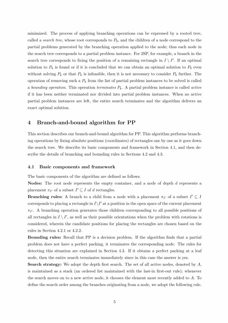
Figure 1. An example of the strip packing problem

2.1 The strip packing problem

Let I = {1, 2, . . . , n} be a set of n rectangles. We are given a width wi and a height hi for

each rectangle i ∈ I and a width W for a strip. The strip packing problem requires that n

rectangles be placed without overlap into the strip so as to minimize the height H of the strip.

We designate the bottom left corner of the strip as the origin of the xy-plane, letting the x-axis

be the direction of the width of the strip, and the y-axis be the direction of the height. We

3

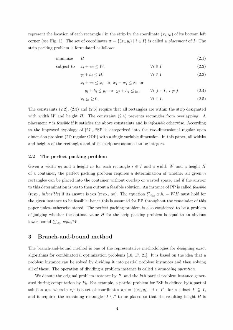
represent the location of each rectangle i in the strip by the coordinate (xi, yi) of its bottom left

corner (see Fig. 1). The set of coordinates π = {(xi, yi) | i ∈ I} is called a placement of I. The

strip packing problem is formulated as follows:

minimize H (2.1)

subject to xi + wi ≤ W, ∀i ∈ I (2.2)

yi + hi ≤ H, ∀i ∈ I (2.3)

xi + wi ≤ xj or xj + wj ≤ xi or

yi + hi ≤ yj or yj + hj ≤ yi, ∀i, j ∈ I, i �= j (2.4)

xi, yi ≥ 0, ∀i ∈ I. (2.5)

The constraints (2.2), (2.3) and (2.5) require that all rectangles are within the strip designated

with width W and height H. The constraint (2.4) prevents rectangles from overlapping. A

placement π is feasible if it satisfies the above constraints and is infeasible otherwise. According

to the improved typology of [27], 2SP is categorized into the two-dimensional regular open

dimension problem (2D regular ODP) with a single variable dimension. In this paper, all widths

and heights of the rectangles and of the strip are assumed to be integers.

2.2 The perfect packing problem

Given a width wi and a height hi for each rectangle i ∈ I and a width W and a height H

of a container, the perfect packing problem requires a determination of whether all given n

rectangles can be placed into the container without overlap or wasted space, and if the answer

to this determination is yes to then output a feasible solution. An instance of PP is called feasible

(resp., infeasible) if its answer is yes (resp., no). The equation∑

i∈I wihi = WH must hold for

the given instance to be feasible; hence this is assumed for PP throughout the remainder of this

paper unless otherwise stated. The perfect packing problem is also considered to be a problem

of judging whether the optimal value H for the strip packing problem is equal to an obvious

lower bound∑

i∈I wihi/W .

3 Branch-and-bound method

The branch-and-bound method is one of the representative methodologies for designing exact

algorithms for combinatorial optimization problems [10, 17, 21]. It is based on the idea that a

problem instance can be solved by dividing it into partial problem instances and then solving

all of those. The operation of dividing a problem instance is called a branching operation.

We denote the original problem instance by P0 and the kth partial problem instance gener-

ated during computation by Pk. For example, a partial problem for 2SP is defined by a partial

solution πI′ , wherein πI′ is a set of coordinates πI′ = {(xi, yi) | i ∈ I ′} for a subset I ′ ⊆ I,

and it requires the remaining rectangles I \ I ′ to be placed so that the resulting height H is

4

minimized. The process of applying branching operations can be expressed by a rooted tree,

called a search tree, whose root corresponds to P0, and the children of a node correspond to the

partial problems generated by the branching operation applied to the node; thus each node in

the search tree corresponds to a partial problem instance. For 2SP, for example, a branch in the

search tree corresponds to fixing the position of a remaining rectangle in I \ I ′. If an optimal

solution to Pk is found or if it is concluded that we can obtain an optimal solution to P0 even

without solving Pk or that Pk is infeasible, then it is not necessary to consider Pk further. The

operation of removing such a Pk from the list of partial problem instances to be solved is called

a bounding operation. This operation terminates Pk. A partial problem instance is called active

if it has been neither terminated nor divided into partial problem instances. When no active

partial problem instances are left, the entire search terminates and the algorithm delivers an

exact optimal solution.

4 Branch-and-bound algorithm for PP

This section describes our branch-and-bound algorithm for PP. This algorithm performs branch-

ing operations by fixing absolute positions (coordinates) of rectangles one by one as it goes down

the search tree. We describe its basic components and framework in Section 4.1, and then de-

scribe the details of branching and bounding rules in Sections 4.2 and 4.3.

4.1 Basic components and framework

The basic components of the algorithm are defined as follows.

Nodes: The root node represents the empty container, and a node of depth d represents a

placement πI′ of a subset I ′ ⊆ I of d rectangles.

Branching rules: A branch to a child from a node with a placement πI′ of a subset I ′ ⊆ I

corresponds to placing a rectangle in I\I ′ at a position in the open space of the current placement

πI′ . A branching operation generates those children corresponding to all possible positions of

all rectangles in I \ I ′, as well as their possible orientations when the problem with rotations is

considered, wherein the candidate positions for placing the rectangles are chosen based on the

rules in Section 4.2.1 or 4.2.2.

Bounding rules: Recall that PP is a decision problem. If the algorithm finds that a partial

problem does not have a perfect packing, it terminates the corresponding node. The rules for

detecting this situation are explained in Section 4.3. If it obtains a perfect packing at a leaf

node, then the entire search terminates immediately since in this case the answer is yes.

Search strategy: We adopt the depth first search. The set of all active nodes, denoted by A,

is maintained as a stack (an ordered list maintained with the last-in first-out rule); whenever

the search moves on to a new active node, it chooses the element most recently added to A. To

define the search order among the branches originating from a node, we adopt the following rule.

5

Prior to our algorithm starting a search, it will sort the given rectangles by non-increasing area

(breaking ties by non-increasing width) and will renumber the indices according to this order.

When a branching operation generates the children of a node, it adds the generated children to

A in decreasing order of indices of the rectangles corresponding to the branches. This means

that a branch with a rectangle with a smaller index is searched earlier than those with larger

indices. We confirmed through preliminary experiments that this strategy is effective for most

instances.

The entire framework of the branch-and-bound algorithm for PP, called algorithm BB-PP,

is formally described as follows.

Algorithm BB-PP

Step 0 (initialization). Sort a given set I of rectangles in the order of non-increasing areas

(breaking ties by non-increasing width) and renumber the indices according to this order.

Let A := {the original instance}.Step 1 (judgement). If A is empty, then output ‘infeasible’ and stop. Otherwise, let u ∈ A

be the node most recently added to A, and then let A := A\{u}. Let πu be the placement

corresponding to u. If πu is a perfect packing of I, then output ‘feasible’ and stop.

Step 2 (bounding operation). If πu is a placement of whole I (this means that πu is infea-

sible), or if u is terminated by one of the bounding rules in Section 4.3, then return to

Step 1. (It is not necessary to use all bounding rules. We examine various combinations

in Section 6.)

Step 3 (branching operation). Generate the children of u based on a branching rule in Sec-

tion 4.2 (BL placement or staircase placement), and add the generated nodes to A in the

decreasing order of indices of the placed rectangles. Return to Step 1.

4.2 Branching rules

We consider two branching rules, one based on the bottom left point and the other based on

a staircase placement, which will be explained in Sections 4.2.1 and 4.2.2, respectively. Let

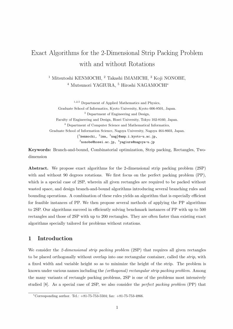
B = [0, W ]× [0, H] denote the set of all points inside or on the boundary of the container. For a

placement π = {(xi, yi) | i ∈ I ′} of a subset I ′ ⊆ I, let Cπ = {(x, y) | xi ≤ x ≤ xi + wi and yi ≤y ≤ yi + hi for some i ∈ I ′} denote the set of points inside the placed rectangles or on their

boundaries. Let Uπ = B \Cπ, and cl(Uπ) denote the closure of Uπ, i.e., the minimum closed set

including Uπ (see Fig. 2(a)).

4.2.1 Branching based on the bottom left point

We first explain the branching based on the bottom left placement for the case without rotations.

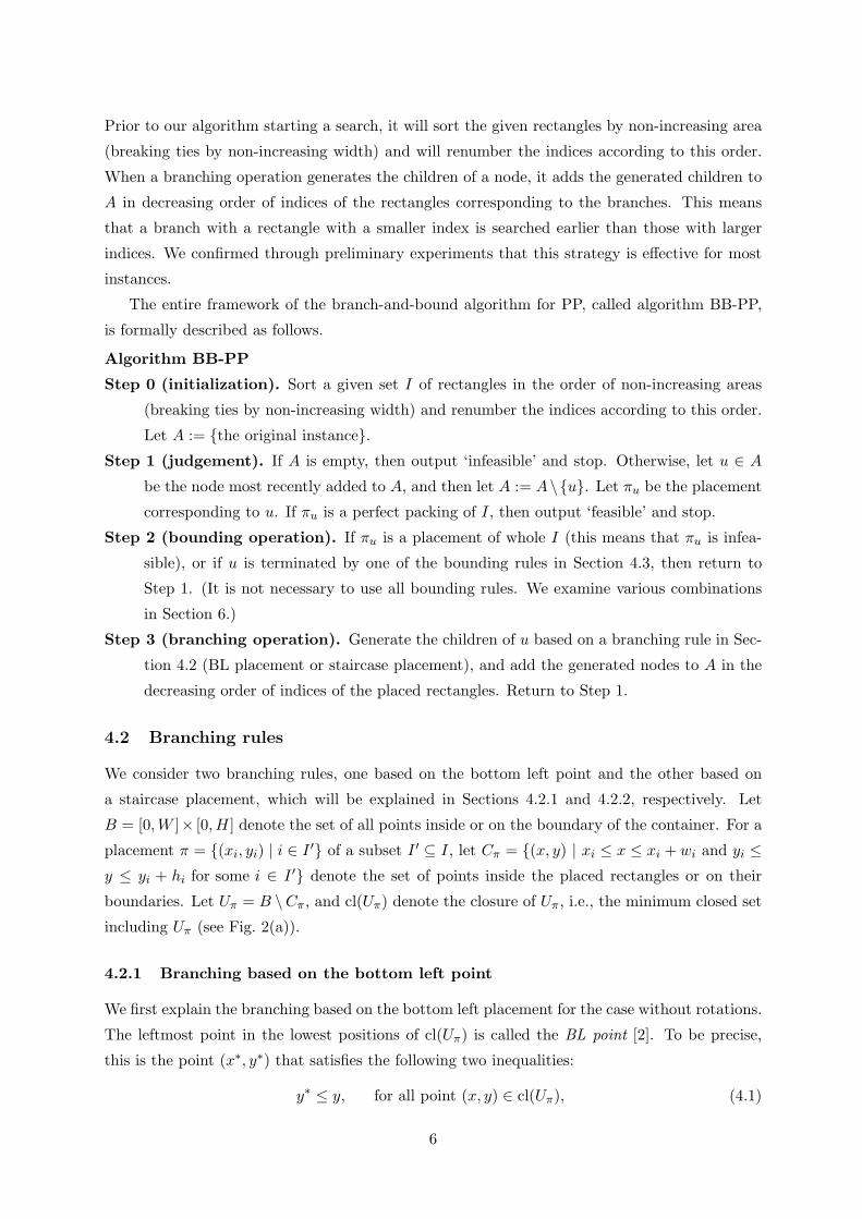
The leftmost point in the lowest positions of cl(Uπ) is called the BL point [2]. To be precise,

this is the point (x∗, y∗) that satisfies the following two inequalities:

y∗ ≤ y, for all point (x, y) ∈ cl(Uπ), (4.1)

6

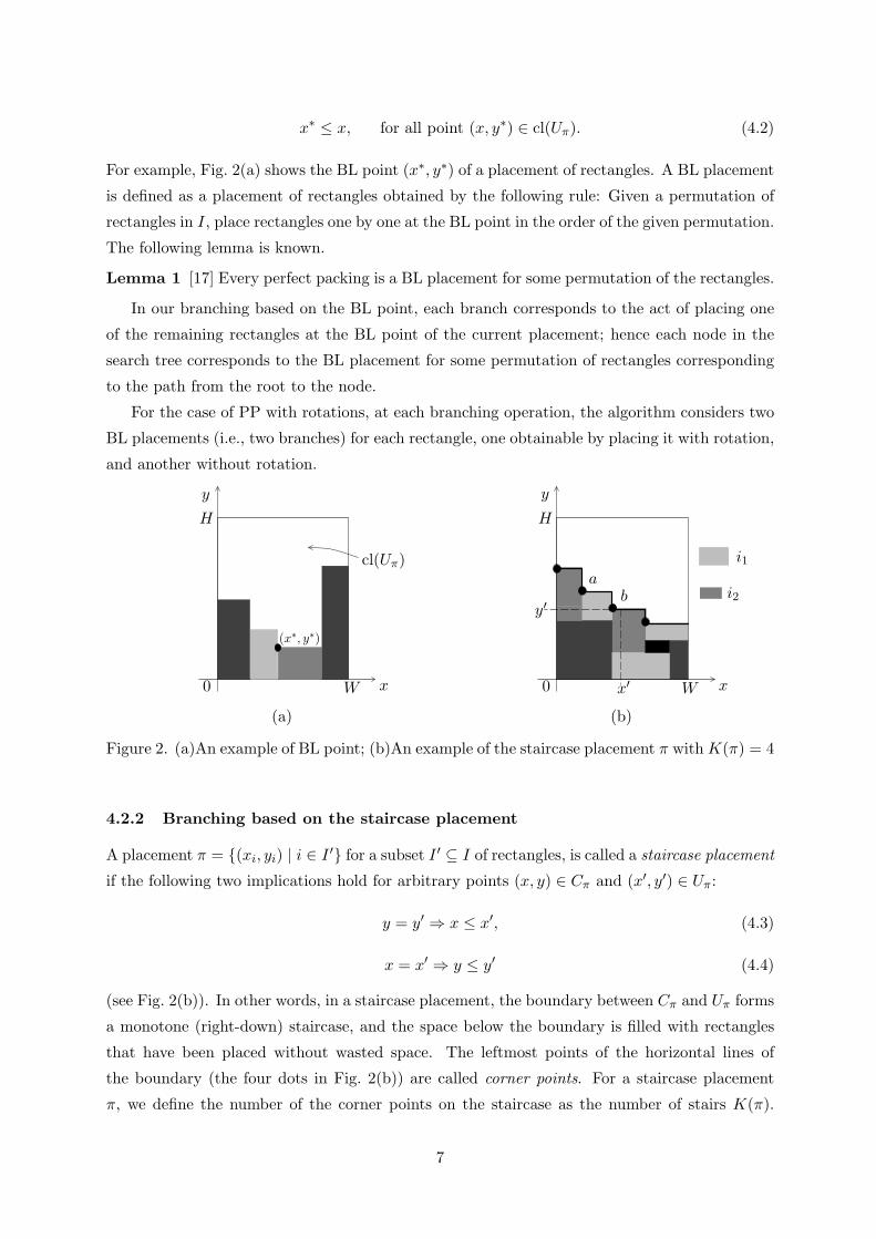
x∗ ≤ x, for all point (x, y∗) ∈ cl(Uπ). (4.2)

For example, Fig. 2(a) shows the BL point (x∗, y∗) of a placement of rectangles. A BL placement

is defined as a placement of rectangles obtained by the following rule: Given a permutation of

rectangles in I, place rectangles one by one at the BL point in the order of the given permutation.

The following lemma is known.

Lemma 1 [17] Every perfect packing is a BL placement for some permutation of the rectangles.

In our branching based on the BL point, each branch corresponds to the act of placing one

of the remaining rectangles at the BL point of the current placement; hence each node in the

search tree corresponds to the BL placement for some permutation of rectangles corresponding

to the path from the root to the node.

For the case of PP with rotations, at each branching operation, the algorithm considers two

BL placements (i.e., two branches) for each rectangle, one obtainable by placing it with rotation,

and another without rotation.

0 x

y

W

H

(x∗, y∗)

cl(Uπ)

(a)

0 x

y

W

H

x′

y′

ab

i1

i2

(b)

Figure 2. (a)An example of BL point; (b)An example of the staircase placement π with K(π) = 4

4.2.2 Branching based on the staircase placement

A placement π = {(xi, yi) | i ∈ I ′} for a subset I ′ ⊆ I of rectangles, is called a staircase placement

if the following two implications hold for arbitrary points (x, y) ∈ Cπ and (x′, y′) ∈ Uπ:

y = y′ ⇒ x ≤ x′, (4.3)

x = x′ ⇒ y ≤ y′ (4.4)

(see Fig. 2(b)). In other words, in a staircase placement, the boundary between Cπ and Uπ forms

a monotone (right-down) staircase, and the space below the boundary is filled with rectangles

that have been placed without wasted space. The leftmost points of the horizontal lines of

the boundary (the four dots in Fig. 2(b)) are called corner points. For a staircase placement

π, we define the number of the corner points on the staircase as the number of stairs K(π).

7

The algorithm performs branching operations by placing rectangles at corner points, keeping

the placement as a staircase placement. Therefore, in a search tree based on this branching

operation, a node v is a child of a node u if and only if v corresponds to a staircase placement πv

that is obtainable by placing one of the remaining rectangles at a corner point of the placement

πu of u. It is not difficult to see that the correctness of this branching operation is derived from

the following lemma:

Lemma 2 For any staircase placement with at least one rectangle, there exists a rectangle such

that the two conditions (4.3) and (4.4) hold even after its removal.

Since the number of stairs K(π) is less than or equal to n/2� for any staircase placement

obtained from a perfect packing of I by Lemma 2, we do not generate any placement such

that the number of stairs is more than n/2�. The idea of using staircase placements was first

proposed in [22] in a more general form for 2SP.

In the case of PP with rotations, we consider placements of each rectangle both with and

without rotation at each corner point.

Limitation on the number of stairs

Perfect placements sometimes consist of several compound rectangles, and such placements do

not require many stairs to place rectangles with the staircase placement strategy. To find such

placements more quickly, we introduce the following heuristic rule. We set an upper limit κ

on the number of stairs during the search; i.e., if a generated node corresponds to a staircase

placement π whose number of stairs is K(π) > κ, then we terminate the node immediately. If

a given instance is feasible, a feasible solution is often found more quickly using this heuristic

rule [24]. When initiating this heuristic, we first set κ = 2. If the search terminates all active

nodes without finding a feasible placement with the current limit κ, then we increase the limit by

one. We repeat this process until κ becomes 4. If we are unable to find a feasible solution with

κ = 4, we increase the limit κ to n/2�, which is equivalent to the case with no limitation on

K(π). If no feasible solution is found even with κ = n/2�, then we conclude that the instance

is infeasible.

Redundancy check

Branching based on the staircase placement may generate two nodes u, v which correspond to

the same placement πu = πv. For example, consider two corner points a, b of a placement π

for I ′ ⊆ I and two rectangles i1, i2 ∈ I \ I ′ (see Fig. 2(b)). The node u generated by placing

rectangle i1 at a after placing rectangle i2 at b and the node v generated by placing rectangle

i2 at b after placing rectangle i1 at a are descendants of the node for π, and have the same

placement πu = πv. Below are some techniques we use to reduce such redundancy.

For each rectangle r ∈ I, we introduce a list Lr that stores the positions already searched,

and check the list whenever we place rectangle r. This technique is also used in [21], but we

8

have modified it for use with our algorithms as follows: If there are rectangles i and j whose

shapes are same (i.e., wi = wj and hi = hj), then they share the same list.

Moreover, we maintain another list that stores all the searched placements with a small

number of stairs (to a maximum of two stairs). We check the list whenever the number of stairs

K(πv) of the placement πv of the current node v with rectangle set I ′ is less than or equal to

two. If the list contains a placement π for the same I ′ and all the coordinates of corner points

of π and πv are the same, then we terminate the node v.

4.3 Bounding operations

This subsection describes three rules for bounding operations: the dynamic programming cut

(DP cut), the bounding rule based on the staircase placement and the remaining rectangles, and

the LP cut, which are explained in Sections 4.3.1, 4.3.2 and 4.3.3, respectively.

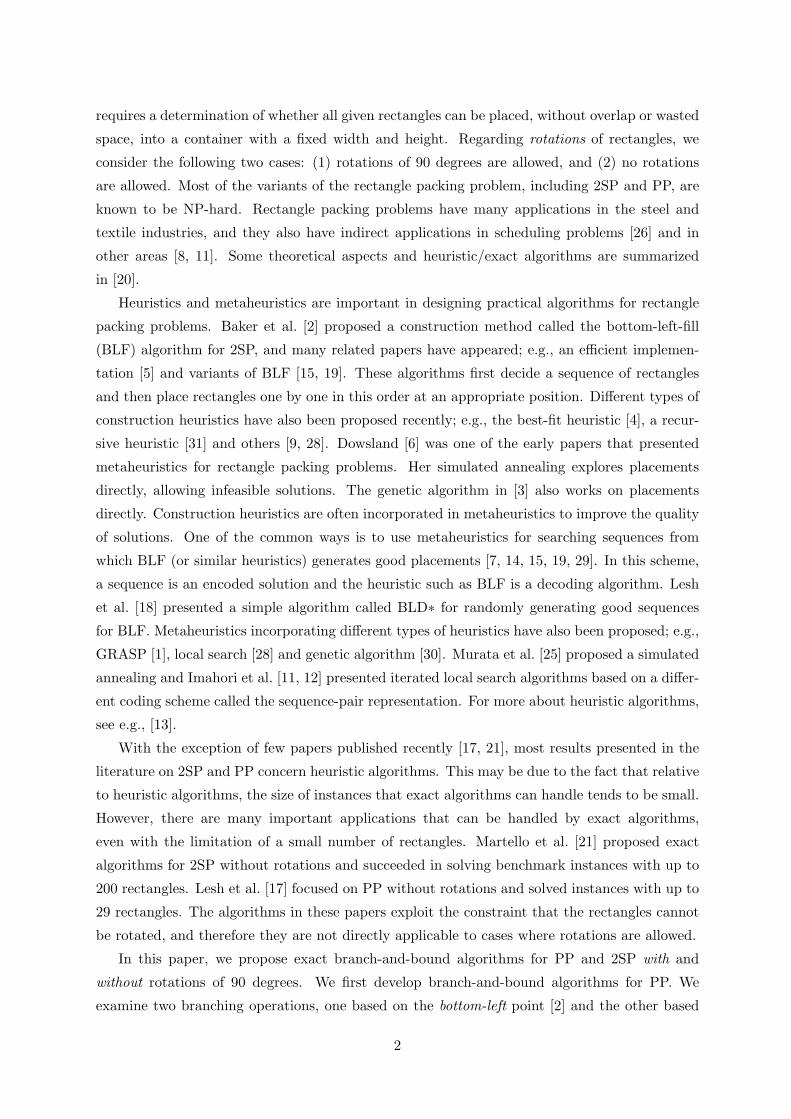
4.3.1 Dynamic programming cut (DP cut)

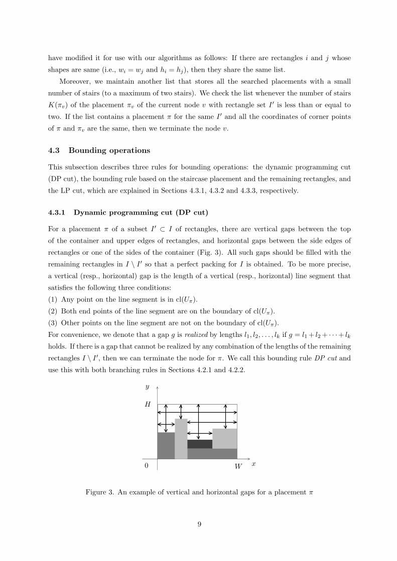
For a placement π of a subset I ′ ⊂ I of rectangles, there are vertical gaps between the top

of the container and upper edges of rectangles, and horizontal gaps between the side edges of

rectangles or one of the sides of the container (Fig. 3). All such gaps should be filled with the

remaining rectangles in I \ I ′ so that a perfect packing for I is obtained. To be more precise,

a vertical (resp., horizontal) gap is the length of a vertical (resp., horizontal) line segment that

satisfies the following three conditions:

(1) Any point on the line segment is in cl(Uπ).

(2) Both end points of the line segment are on the boundary of cl(Uπ).

(3) Other points on the line segment are not on the boundary of cl(Uπ).

For convenience, we denote that a gap g is realized by lengths l1, l2, . . . , lk if g = l1 + l2 + · · ·+ lk

holds. If there is a gap that cannot be realized by any combination of the lengths of the remaining

rectangles I \ I ′, then we can terminate the node for π. We call this bounding rule DP cut and

use this with both branching rules in Sections 4.2.1 and 4.2.2.

0 x

y

W

H

Figure 3. An example of vertical and horizontal gaps for a placement π

9

We compute whether each of the gaps can be realized by a combination of the lengths,

wi, hi, i ∈ I \ I ′, in the following way. We first consider the case with rotations. For a given

placement π = {(xi, yi) | i ∈ I ′}, we denote the remaining rectangles in I \ I ′ by i = 1, 2, . . . , m

for simplicity. The problem of judging whether a given gap can be filled is formulated as a

problem similar to the subset sum problem, and it can be solved by using dynamic programming

(DP) [23]. Let zri (resp., zu

i ) be a 0,1-variable that takes value 1 if we use the rotated (resp.,

unrotated) rectangle i to fill the gap, and 0 otherwise. Then, for t = 1, 2, . . . , m and an integer

p ≥ 0, the problem Qt(p) of finding a combination of rectangles from {1, 2, . . . , t} that realizes

vertical gap p ≥ 0 is formally described as follows:

Qt(p) Find z = (zr1, z

r2, . . . , z

rt , z

u1 , zu

2 , . . . , zut ) (4.5)

such thatt∑

i=1

(wizri + hiz

ui ) = p (4.6)

zri + zu

i ≤ 1, ∀i = 1, 2, . . . , t (4.7)

zri , z

ui ∈ {0, 1}, ∀i = 1, 2, . . . , t. (4.8)

(Note that, though our objective is to find a solution to Qm(p), for convenience we define the

problem for all t ≤ m.) Let vt(p) be 1 if there exists a solution to Qt(p) and 0 otherwise.

Lemma 3 All vt(p), t = 1, 2, . . . , m can be computed in O(m(W + H)) time.

Proof. We can compute vt(p) by

v0(p) =

⎧⎨⎩

1, p = 0,

0, otherwise,(4.9)

vt(p) = max{vt−1(p), vt−1(p − wt), vt−1(p − ht)}, (4.10)

t = 1, 2, . . . , m,

where (4.9) is the boundary condition that represents trivial cases with the empty set of rect-

angles. Note that by definition vt(p) = 0 holds for any p < 0.

Note that a single run of the above algorithm suffices to find the feasibility of all vertical

gaps. The same algorithm can also judge the feasibility of horizontal gaps just by exchanging

the roles of variables zri and zu

i . We can therefore compute the feasibility of all vertical and

horizontal gaps by a single run of the above DP recursion. Though we define vt(p) for all

nonnegative integers p, we only need to calculate it for p = 0, 1, . . . ,max {W, H}. Hence the

above recurrence formula can be calculated in O(m(W + H)) time.

In the case of the problem without rotations, the problem becomes equivalent to the subset

sum problem, and we only need to independently execute similar DPs for the horizontal and

vertical gaps. When we calculate the DP for the vertical (resp., horizontal) gaps, we remove the

second term vt−1(p−wt) (resp., the third term vt−1(p−ht)) from the recurrence formula (4.10).

A similar idea is also used in [17], where only horizontal gaps are considered and upper

bounds on the possible height of the gap are computed based on a slightly more complicated

10

DP recursion. We simplify their DP, not considering the height but using 0,1-variables, in order

to apply it to the case with rotations.

Adaptive control of DP cut

Through preliminary experiments we observed that when the depth of the node in a search

tree is relatively small DP cut often fails in terminating nodes. Since executing DP cut is

computationally expensive, we incorporate a mechanism to control timing for invoking the DP

cut procedure. For this, we use a variable β. We invoke DP cut only if the depth d of the

current node satisfies d ≥ β. We control the variable β using two constant parameters δ and q

as follows. We set β := 0 at the root node. Whenever we succeed in terminating a node by a

DP cut, we reduce β to max{β − δ, 0}. When the DP cut procedure fails in terminating nodes q

consecutive times, we increase β by 1. We use δ = 1 and q = 4 in the computational experiments

in Section 6.

4.3.2 The bounding rule based on the staircase placement and the remaining rect-

angles

We introduce three simple bounding rules, which are applicable only in branching based on

the staircase placement strategy. We terminate the node corresponding to a placement π for

I ′ immediately if one of the following conditions is satisfied: (I) The number of the remaining

rectangles |I \ I ′| is smaller than the number of corner points of π. (II) There is a rectangle r

in I \ I ′ which cannot be placed at any corner point of the staircase of π without protruding

from the container. (III) All the indices of the remaining rectangles I \ I ′ are smaller than the

index of the rectangle placed at the origin (0, 0). The third condition indicates that we have

already checked all possible staircase placements formed by I \ I ′ and failed in finding a perfect

packing. Hence none of these placements can have the same shape as that of cl(Uπ) rotated by

180 degrees.

4.3.3 LP cut

Formulating PP as an integer programming problem, we consider a bounding operation based

on its linear programming (LP) relaxation. This operation is applicable to both branching

strategies in Sections 4.2.1 and 4.2.2.

We first explain the case with rotations. We define variables zui,x,y and zr

i,x,y for i ∈ I and

(x, y) ∈ B = {0, 1, . . . , W} × {0, 1, . . . , H}, where their meanings are as follows:

• zui,x,y = 1 if rectangle i is placed at (x, y) without rotation, and 0 otherwise.

• zri,x,y = 1 if rectangle i is placed at (x, y) with rotation, and 0 otherwise.

Moreover, we define Bui = {(x, y) | x = 0, 1, . . . , W − wi, y = 0, 1, . . . , H − hi} and Br

i =

{(x, y) | x = 0, 1, . . . , W − hi, y = 0, 1, . . . , H − wi} for each i ∈ I. Then PP can be formulated

11

as the following integer program:

maximize∑i∈I

∑(x,y)∈Bu

i

zui,x,y +

∑i∈I

∑(x,y)∈Br

i

zri,x,y (4.11)

subject to∑

(x,y)∈Bui

zui,x,y +

∑(x,y)∈Br

i

zri,x,y ≤ 1, ∀i ∈ I (4.12)

∑i∈I

∑x−wi<x′≤x

y−hi<y′≤y

zui,x′,y′+

∑i∈I

∑x−hi<x′≤x

y−wi<y′≤y

zri,x′,y′ ≤1, ∀(x, y) ∈ B (4.13)

zui,x,y, z

ri,x,y ∈ {0, 1}, ∀i ∈ I, (x, y) ∈ B (4.14)

zui,x,y = 0, ∀i ∈ I, (x, y) /∈ Bu

i (4.15)

zri,x,y = 0, ∀i ∈ I, (x, y) /∈ Br

i . (4.16)

The constraint (4.12) means that each rectangle cannot be placed more than once and (4.13)

means that no rectangles can overlap. The original instance for PP has a perfect packing if and

only if the optimal value of the corresponding instance of this problem is equal to n.

We now consider the LP relaxation of this problem by relaxing constraints zui,x,y, z

ri,x,y ∈ {0, 1}

to 0 ≤ zui,x,y, z

ri,x,y ≤ 1 for all i ∈ I and (x, y) ∈ B.

Lemma 4 For a given placement π = {(xi, yi) | i ∈ I ′} of rectangles, fix the variables zui,x,y, z

ri,x,y

for the placed rectangles i ∈ I ′ accordingly. If the optimal value of the resulting LP instance is

less than n, then no perfect packing of I is obtained by extending π.

This formulation contains Ω(nWH) variables and WH +n constraints. Hence this bounding

rule is not practical for problem instances with relatively large WH.

We can also utilize an LP relaxation for the case without rotations. In this case, variables

zri,x,y are fixed at 0, and therefore are not necessarily introduced in this formulation.

5 Application of PP algorithms to 2SP

This section gives some ideas on applying the algorithms from the previous section to 2SP. We

first explain the reduction from 2SP to PP in Section 5.1 and then introduce generalizations of

staircase placement, DP cut, and the bounding rule based on the staircase placement and the

remaining rectangles in Sections 5.2, 5.3 and 5.4, respectively. We then propose two algorithms

for 2SP in Section 5.5.

5.1 Reduction from 2SP to PP

For a given 2SP instance with a set I of rectangles, let H ′ be an integer such that WH ′ ≥∑i∈I wihi. The optimal value of the 2SP instance is less than or equal to H ′ if and only if the

following PP instance is feasible. We set the height of the container to H ′ and add WH ′−∑i wihi

new 1×1 rectangles to the set I so that equation∑

wihi = WH ′ holds for the resulting instance,

where “1 × 1” means that its height and width are 1.

12

0 x

y

W

H

Vπ

Dπ

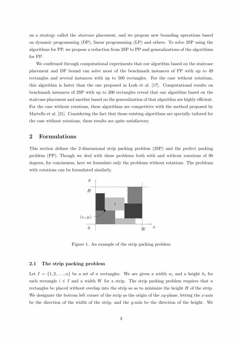
Figure 4. Generalized definition of staircase

Given our assumption that all widths and heights of rectangles are integers, the optimal

value of 2SP is also an integer. Hence, 2SP is equivalent to determining the minimum H ′ such

that the corresponding PP instance has a perfect packing.

5.2 Generalizations of staircase placement

Adding too many 1 × 1 rectangles could lead to a redundant search. We therefore consider

an additional idea to generalize the staircase placement. The space below the boundary of a

staircase placement must be filled with rectangles placed without wasted space in the original

definition in Section 4.2.2. Here we generalize the definition so that it allows wasted space in the

space below the boundary. For a given placement π of I ′, let Vπ := {(x′, y′) ∈ Uπ | both (4.3) and

(4.4) holds for arbitrary (x, y) ∈ Cπ} and we call cl(Dπ) for Dπ := Uπ \Vπ the abandoned space,

where Cπ and Uπ are defined as in Section 4.2. Then (4.3) and (4.4) hold for arbitrary points

(x, y) ∈ Cπ ∪ Dπ and (x′, y′) ∈ Vπ. The boundary cl(Cπ ∪ Dπ) ∩ cl(Vπ) becomes a right-down

staircase by this definition as shown in thick lines in Fig. 4, where the gray area is the placed

rectangles of I ′. As in the original staircase, the number of stairs K(π) is the number of corner

points of the generalized staircase.

As in the branching operation based on the original staircase placement, the algorithm does

not put any remaining rectangle into the space below the boundary in the descendants of the

search tree; it puts them only at corner points of the staircase. The validity of this branching

operation is proved in [22].

5.3 Extension of DP cut

DP cut can be applied directly to 2SP if we adopt the strategy introduced in Section 5.1; i.e.,

if we calculate DP after adding 1 × 1 rectangles. However, as the number of 1 × 1 rectangles

increases, gaps are more easily realized and the DP cut becomes less effective. To alleviate this,

we propose a new idea of executing the DP computation without 1 × 1 rectangles explicitly.

For a given placement π of I ′, let gvk (resp., gh

k) be the length of the kth shortest vertical gap

13

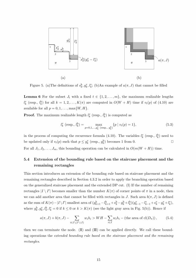
(resp., the kth longest horizontal gap ghk) in π (k = 1, 2, . . . , K(π)), and sh

k (resp., svk) be the

width (resp., height) of the stair which forms the boundary of the gap in π (see Fig. 5(a)). Let

J be a subset of I \ I ′. We then compute lvk (resp., lhk), the maximum realizable length by some

combination of the lengths of the rectangles in J less than or equal to gvk (resp., gh

k). Then

shk(gv

k − lvk) (resp., svk(g

hk − lhk)) gives a lower bound on the area in Vπ that cannot be filled with

any combination of rectangles in J . When we sum such areas shk(gv

k − lvk) over all vertical gaps

and svk(g

hk − lhk) over all horizontal gaps, we need to subtract the common area (gv

k − lvk)(ghk − lhk)

since this space is computed twice. Moreover, (gvk − lvk)(gh

k+1− lhk+1), k = 1, 2, . . . , K(π)−1 gives

another area that cannot be filled with rectangles in J . We show that the total of the area,

depicted in dark gray in Fig. 5(b), is a lower bound on the area in Vπ that cannot be filled with

any combination of the rectangles in J .

Lemma 5 For a staircase placement π of I ′ and a subset J ⊆ I \ I ′ of the remaining rectangles,

let gvk (resp., gh

k) be the length of the kth shortest vertical gap (resp., the kth longest horizontal

gap), and let lvk (resp., lhk) be the maximum realizable length less than or equal to gvk (resp., gh

k).

Then

a(π, J) =K(π)∑k=1

{shk(gv

k−lvk)+svk(g

hk −lhk)−(gv

k−lvk)(ghk −lhk)}+

K(π)−1∑k=1

{(gvk−lvk)(gh

k+1−lhk+1)} (5.1)

gives a lower bound on the area in Vπ that cannot be filled with any combination of the rectangles

in J .

Proof. Consider a staircase placement π and any feasible placement consisting of a set J ′ ⊆ J

of the rectangles placed in Vπ. Without loss of generality, we assume that all the positions of the

rectangles of J ′ are rightmost and uppermost, i.e., none of the rectangles in J ′ can be translated

rightward or upward without overlapping with other rectangles in J ′ or without protruding from

the container. Then no rectangles can overlap with the area of a(π, J), the dark gray area of

Fig. 5(b), because if there exists such a rectangle, then the length from the top edge (resp., right

edge) of the container to the bottom edge (the left edge) of the rectangle, which is now realizable

with the rectangles in J , would be longer than the maximum realizable length gvk (resp., gh

k).

The area is computed by∑K(π)

k=1 {shk(gv

k − lvk) + svk(g

hk − lhk)− (gv

k − lvk)(ghk − lhk)}+

∑K(π)−1k=1 {(gv

k −lvk)(gh

k+1 − lhk+1)}.Hence if

a(π, J) −∑

i∈I\(I′∪J)

wihi > WH −∑i∈I

wihi − (the area of cl(Dπ)) , (5.2)

then we can terminate the node. We call this bounding operation extended DP cut.

Now, let us turn to the computation of the maximum realizable length lvk (resp., lhk). Let the

remaining rectangles except for the added 1 × 1 rectangles be i = 1, 2, . . . , m for simplicity. We

consider J1 = {1}, J2 = {1, 2}, . . . , Jm = {1, 2, . . . , m} as the candidates of subset J . Then we

have the following lemma.

14

1

2

3

sv2 sh

2

gv3 lv3

sh3(g

v3 − lv3)

π

(a)

1

2

3πa(π, J)

(b)

Figure 5. (a)The definitions of shk, gv

k , lvk; (b)An example of a(π, J) that cannot be filled

Lemma 6 For the subset Jt with a fixed t ∈ {1, 2, . . . , m}, the maximum realizable lengths

lvk (resp., lhk) for all k = 1, 2, . . . , K(π) are computed in O(W + H) time if vt(p) of (4.10) are

available for all p = 0, 1, . . . ,max{W, H}.Proof. The maximum realizable length lvk (resp., lhk) is computed as

lvk (resp., lhk) = maxp=0,1,...,gv

k(resp., gh

k){p | vt(p) = 1}, (5.3)

in the process of computing the recurrence formula (4.10). The variables lvk (resp., lhk) need to

be updated only if vt(p) such that p ≤ gvk (resp., gh

k) becomes 1 from 0.

For all J1, J2, . . . , Jm, this bounding operation can be calculated in O(m(W + H)) time.

5.4 Extension of the bounding rule based on the staircase placement and the

remaining rectangles

This section introduces an extension of the bounding rule based on staircase placement and the

remaining rectangles described in Section 4.3.2 in order to apply the branching operation based

on the generalized staircase placement and the extended DP cut. (I) If the number of remaining

rectangles |I \ I ′| becomes smaller than the number K(π) of corner points of π in a node, then

we can add another area that cannot be filled with rectangles in J . Such area b(π, J) is defined

as the sum of K(π)−|I \I ′| smallest area of (ghk+1− lhk+1 +sh

k−ghk + lhk)(gv

k−1− lvk−1 +svk−gv

k + lvk),

where ghk , gv

k , lhk , lvk = 0 if k ≤ 0 or k > K(π) (see the light gray area in Fig. 5(b)). Hence if

a(π, J) + b(π, J) −∑

i∈I\(I′∪J)

wihi > WH −∑i∈I

wihi − (the area of cl(Dπ)) , (5.4)

then we can terminate the node. (II) and (III) can be applied directly. We call these bound-

ing operations the extended bounding rule based on the staircase placement and the remaining

rectangles.

15

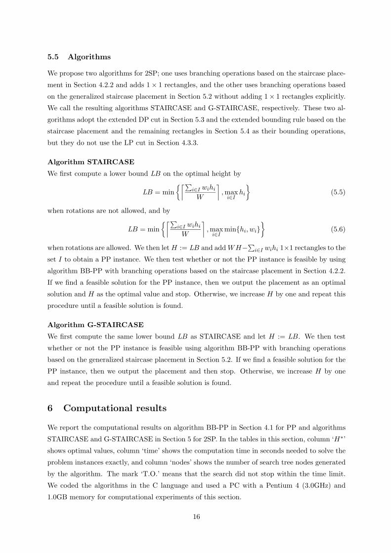
5.5 Algorithms

We propose two algorithms for 2SP; one uses branching operations based on the staircase place-

ment in Section 4.2.2 and adds 1× 1 rectangles, and the other uses branching operations based

on the generalized staircase placement in Section 5.2 without adding 1× 1 rectangles explicitly.

We call the resulting algorithms STAIRCASE and G-STAIRCASE, respectively. These two al-

gorithms adopt the extended DP cut in Section 5.3 and the extended bounding rule based on the

staircase placement and the remaining rectangles in Section 5.4 as their bounding operations,

but they do not use the LP cut in Section 4.3.3.

Algorithm STAIRCASE

We first compute a lower bound LB on the optimal height by

LB = min{⌈∑

i∈I wihi

W

⌉, max

i∈Ihi

}(5.5)

when rotations are not allowed, and by

LB = min{⌈∑

i∈I wihi

W

⌉, max

i∈Imin{hi, wi}

}(5.6)

when rotations are allowed. We then let H := LB and add WH−∑i∈I wihi 1×1 rectangles to the

set I to obtain a PP instance. We then test whether or not the PP instance is feasible by using

algorithm BB-PP with branching operations based on the staircase placement in Section 4.2.2.

If we find a feasible solution for the PP instance, then we output the placement as an optimal

solution and H as the optimal value and stop. Otherwise, we increase H by one and repeat this

procedure until a feasible solution is found.

Algorithm G-STAIRCASE

We first compute the same lower bound LB as STAIRCASE and let H := LB. We then test

whether or not the PP instance is feasible using algorithm BB-PP with branching operations

based on the generalized staircase placement in Section 5.2. If we find a feasible solution for the

PP instance, then we output the placement and then stop. Otherwise, we increase H by one

and repeat the procedure until a feasible solution is found.

6 Computational results

We report the computational results on algorithm BB-PP in Section 4.1 for PP and algorithms

STAIRCASE and G-STAIRCASE in Section 5 for 2SP. In the tables in this section, column ‘H∗’

shows optimal values, column ‘time’ shows the computation time in seconds needed to solve the

problem instances exactly, and column ‘nodes’ shows the number of search tree nodes generated

by the algorithm. The mark ‘T.O.’ means that the search did not stop within the time limit.

We coded the algorithms in the C language and used a PC with a Pentium 4 (3.0GHz) and

1.0GB memory for computational experiments of this section.

16

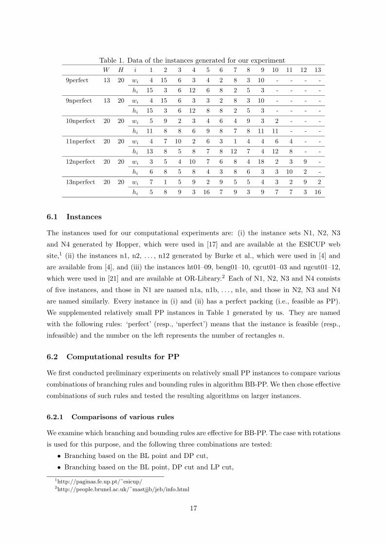
Table 1. Data of the instances generated for our experimentW H i 1 2 3 4 5 6 7 8 9 10 11 12 13

9perfect 13 20 wi 4 15 6 3 4 2 8 3 10 - - - -

hi 15 3 6 12 6 8 2 5 3 - - - -

9nperfect 13 20 wi 4 15 6 3 3 2 8 3 10 - - - -

hi 15 3 6 12 8 8 2 5 3 - - - -

10nperfect 20 20 wi 5 9 2 3 4 6 4 9 3 2 - - -

hi 11 8 8 6 9 8 7 8 11 11 - - -

11nperfect 20 20 wi 4 7 10 2 6 3 1 4 4 6 4 - -

hi 13 8 5 8 7 8 12 7 4 12 8 - -

12nperfect 20 20 wi 3 5 4 10 7 6 8 4 18 2 3 9 -

hi 6 8 5 8 4 3 8 6 3 3 10 2 -

13nperfect 20 20 wi 7 1 5 9 2 9 5 5 4 3 2 9 2

hi 5 8 9 3 16 7 9 3 9 7 7 3 16

6.1 Instances

The instances used for our computational experiments are: (i) the instance sets N1, N2, N3

and N4 generated by Hopper, which were used in [17] and are available at the ESICUP web

site,1 (ii) the instances n1, n2, . . . , n12 generated by Burke et al., which were used in [4] and

are available from [4], and (iii) the instances ht01–09, beng01–10, cgcut01–03 and ngcut01–12,

which were used in [21] and are available at OR-Library.2 Each of N1, N2, N3 and N4 consists

of five instances, and those in N1 are named n1a, n1b, . . . , n1e, and those in N2, N3 and N4

are named similarly. Every instance in (i) and (ii) has a perfect packing (i.e., feasible as PP).

We supplemented relatively small PP instances in Table 1 generated by us. They are named

with the following rules: ‘perfect’ (resp., ‘nperfect’) means that the instance is feasible (resp.,

infeasible) and the number on the left represents the number of rectangles n.

6.2 Computational results for PP

We first conducted preliminary experiments on relatively small PP instances to compare various

combinations of branching rules and bounding rules in algorithm BB-PP. We then chose effective

combinations of such rules and tested the resulting algorithms on larger instances.

6.2.1 Comparisons of various rules

We examine which branching and bounding rules are effective for BB-PP. The case with rotations

is used for this purpose, and the following three combinations are tested:

• Branching based on the BL point and DP cut,

• Branching based on the BL point, DP cut and LP cut,

1http://paginas.fe.up.pt/˜esicup/2http://people.brunel.ac.uk/˜mastjjb/jeb/info.html

17

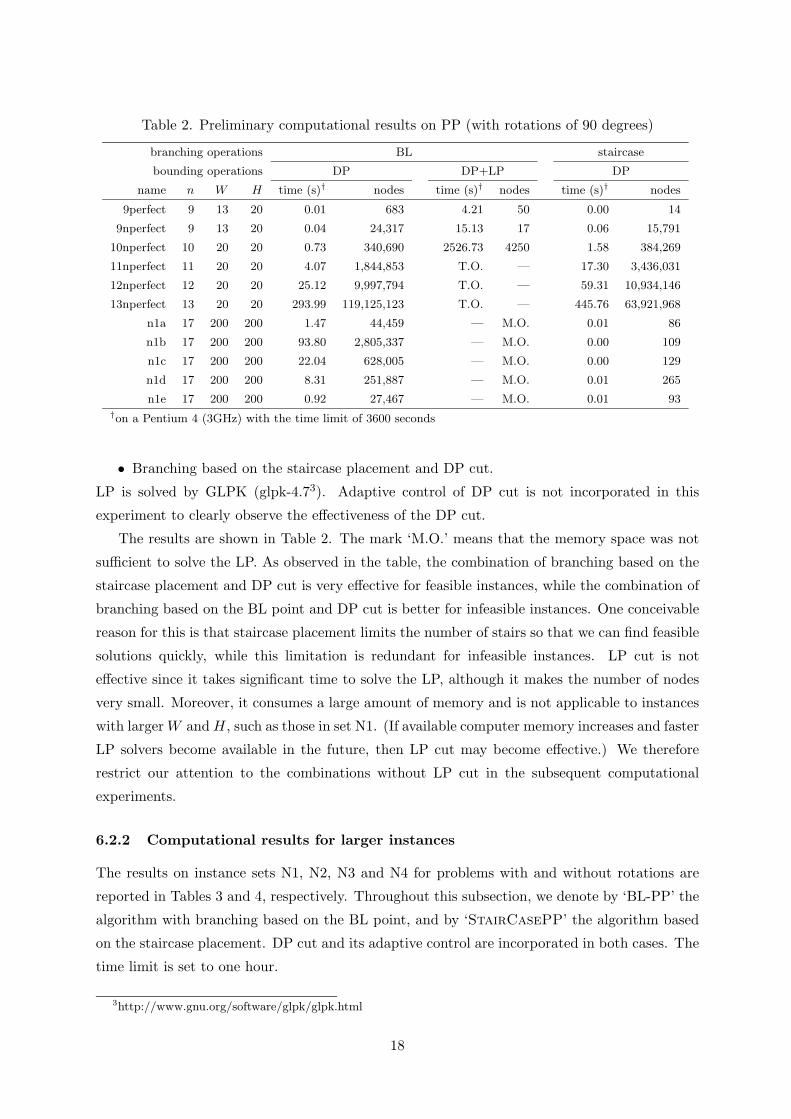
Table 2. Preliminary computational results on PP (with rotations of 90 degrees)

branching operations BL staircase

bounding operations DP DP+LP DP

name n W H time (s)† nodes time (s)† nodes time (s)† nodes

9perfect 9 13 20 0.01 683 4.21 50 0.00 14

9nperfect 9 13 20 0.04 24,317 15.13 17 0.06 15,791

10nperfect 10 20 20 0.73 340,690 2526.73 4250 1.58 384,269

11nperfect 11 20 20 4.07 1,844,853 T.O. — 17.30 3,436,031

12nperfect 12 20 20 25.12 9,997,794 T.O. — 59.31 10,934,146

13nperfect 13 20 20 293.99 119,125,123 T.O. — 445.76 63,921,968

n1a 17 200 200 1.47 44,459 — M.O. 0.01 86

n1b 17 200 200 93.80 2,805,337 — M.O. 0.00 109

n1c 17 200 200 22.04 628,005 — M.O. 0.00 129

n1d 17 200 200 8.31 251,887 — M.O. 0.01 265

n1e 17 200 200 0.92 27,467 — M.O. 0.01 93†on a Pentium 4 (3GHz) with the time limit of 3600 seconds

• Branching based on the staircase placement and DP cut.

LP is solved by GLPK (glpk-4.73). Adaptive control of DP cut is not incorporated in this

experiment to clearly observe the effectiveness of the DP cut.

The results are shown in Table 2. The mark ‘M.O.’ means that the memory space was not

sufficient to solve the LP. As observed in the table, the combination of branching based on the

staircase placement and DP cut is very effective for feasible instances, while the combination of

branching based on the BL point and DP cut is better for infeasible instances. One conceivable

reason for this is that staircase placement limits the number of stairs so that we can find feasible

solutions quickly, while this limitation is redundant for infeasible instances. LP cut is not

effective since it takes significant time to solve the LP, although it makes the number of nodes

very small. Moreover, it consumes a large amount of memory and is not applicable to instances

with larger W and H, such as those in set N1. (If available computer memory increases and faster

LP solvers become available in the future, then LP cut may become effective.) We therefore

restrict our attention to the combinations without LP cut in the subsequent computational

experiments.

6.2.2 Computational results for larger instances

The results on instance sets N1, N2, N3 and N4 for problems with and without rotations are

reported in Tables 3 and 4, respectively. Throughout this subsection, we denote by ‘BL-PP’ the

algorithm with branching based on the BL point, and by ‘StairCasePP’ the algorithm based

on the staircase placement. DP cut and its adaptive control are incorporated in both cases. The

time limit is set to one hour.

3http://www.gnu.org/software/glpk/glpk.html

18

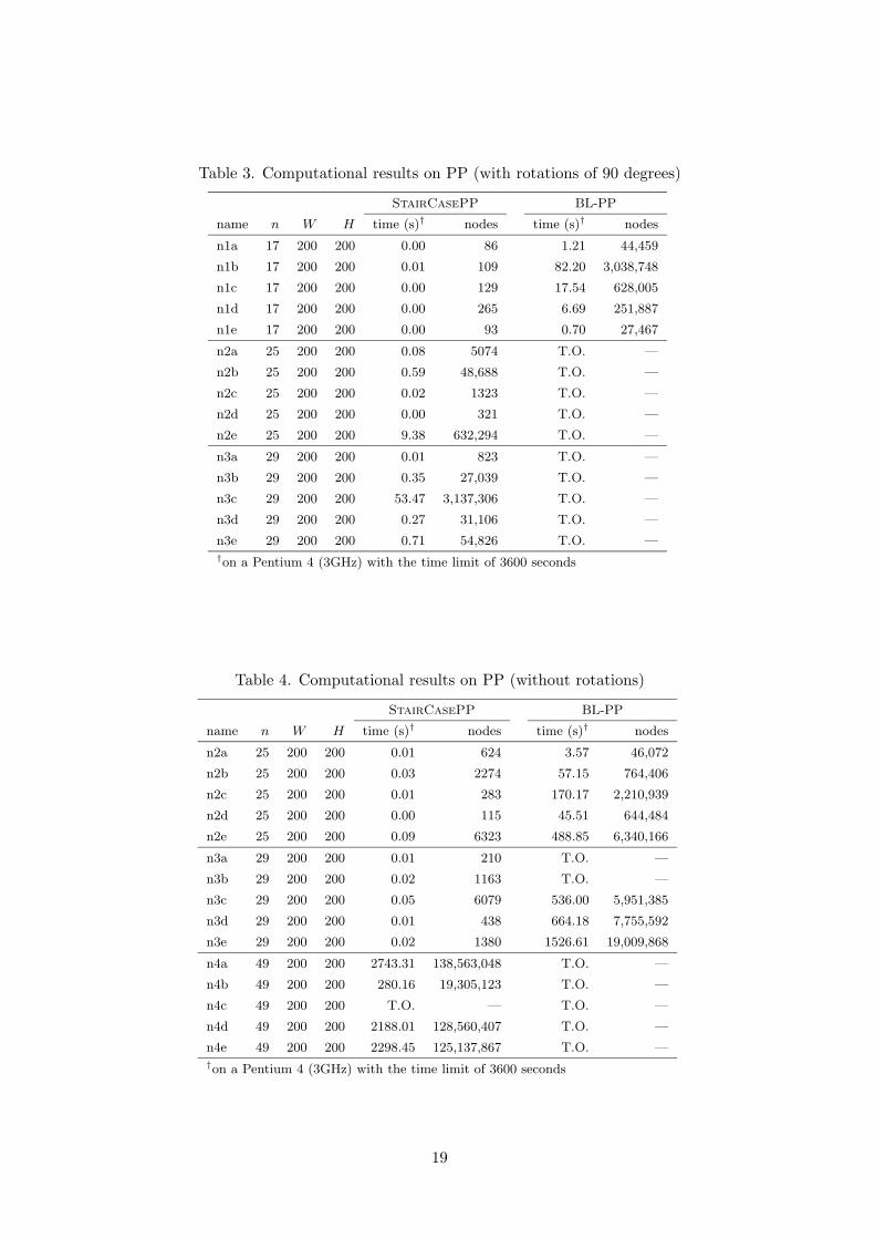
Table 3. Computational results on PP (with rotations of 90 degrees)

StairCasePP BL-PP

name n W H time (s)† nodes time (s)† nodes

n1a 17 200 200 0.00 86 1.21 44,459

n1b 17 200 200 0.01 109 82.20 3,038,748

n1c 17 200 200 0.00 129 17.54 628,005

n1d 17 200 200 0.00 265 6.69 251,887

n1e 17 200 200 0.00 93 0.70 27,467

n2a 25 200 200 0.08 5074 T.O. —

n2b 25 200 200 0.59 48,688 T.O. —

n2c 25 200 200 0.02 1323 T.O. —

n2d 25 200 200 0.00 321 T.O. —

n2e 25 200 200 9.38 632,294 T.O. —

n3a 29 200 200 0.01 823 T.O. —

n3b 29 200 200 0.35 27,039 T.O. —

n3c 29 200 200 53.47 3,137,306 T.O. —

n3d 29 200 200 0.27 31,106 T.O. —

n3e 29 200 200 0.71 54,826 T.O. —†on a Pentium 4 (3GHz) with the time limit of 3600 seconds

Table 4. Computational results on PP (without rotations)

StairCasePP BL-PP

name n W H time (s)† nodes time (s)† nodes

n2a 25 200 200 0.01 624 3.57 46,072

n2b 25 200 200 0.03 2274 57.15 764,406

n2c 25 200 200 0.01 283 170.17 2,210,939

n2d 25 200 200 0.00 115 45.51 644,484

n2e 25 200 200 0.09 6323 488.85 6,340,166

n3a 29 200 200 0.01 210 T.O. —

n3b 29 200 200 0.02 1163 T.O. —

n3c 29 200 200 0.05 6079 536.00 5,951,385

n3d 29 200 200 0.01 438 664.18 7,755,592

n3e 29 200 200 0.02 1380 1526.61 19,009,868

n4a 49 200 200 2743.31 138,563,048 T.O. —

n4b 49 200 200 280.16 19,305,123 T.O. —

n4c 49 200 200 T.O. — T.O. —

n4d 49 200 200 2188.01 128,560,407 T.O. —

n4e 49 200 200 2298.45 125,137,867 T.O. —†on a Pentium 4 (3GHz) with the time limit of 3600 seconds

19

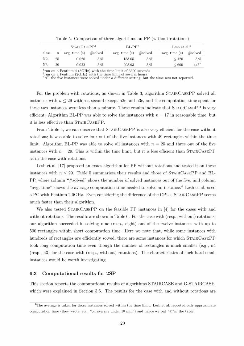
Table 5. Comparison of three algorithms on PP (without rotations)

StairCasePP† BL-PP† Lesh et al.‡

class n avg. time (s) #solved avg. time (s) #solved avg. time (s) #solved

N2 25 0.028 5/5 153.05 5/5 ≤ 120 5/5

N3 29 0.022 5/5 908.93 3/5 ≤ 600 4/5�

†run on a Pentium 4 (3GHz) with the time limit of 3600 seconds‡run on a Pentium (2GHz) with the time limit of several hours�All the five instances were solved under a different setting, but the time was not reported.

For the problem with rotations, as shown in Table 3, algorithm StairCasePP solved all

instances with n ≤ 29 within a second except n2e and n3c, and the computation time spent for

these two instances were less than a minute. These results indicate that StairCasePP is very

efficient. Algorithm BL-PP was able to solve the instances with n = 17 in reasonable time, but

it is less effective than StairCasePP.

From Table 4, we can observe that StairCasePP is also very efficient for the case without

rotations; it was able to solve four out of the five instances with 49 rectangles within the time

limit. Algorithm BL-PP was able to solve all instances with n = 25 and three out of the five

instances with n = 29. This is within the time limit, but it is less efficient than StairCasePP

as in the case with rotations.

Lesh et al. [17] proposed an exact algorithm for PP without rotations and tested it on these

instances with n ≤ 29. Table 5 summarizes their results and those of StairCasePP and BL-

PP, where column “#solved” shows the number of solved instances out of the five, and column

“avg. time” shows the average computation time needed to solve an instance.4 Lesh et al. used

a PC with Pentium 2.0GHz. Even considering the difference of the CPUs, StairCasePP seems

much faster than their algorithm.

We also tested StairCasePP on the feasible PP instances in [4] for the cases with and

without rotations. The results are shown in Table 6. For the case with (resp., without) rotations,

our algorithm succeeded in solving nine (resp., eight) out of the twelve instances with up to

500 rectangles within short computation time. Here we note that, while some instances with

hundreds of rectangles are efficiently solved, there are some instances for which StairCasePP

took long computation time even though the number of rectangles is much smaller (e.g., n4

(resp., n3) for the case with (resp., without) rotations). The characteristics of such hard small

instances would be worth investigating.

6.3 Computational results for 2SP

This section reports the computational results of algorithms STAIRCASE and G-STAIRCASE,

which were explained in Section 5.5. The results for the case with and without rotations are

4The average is taken for those instances solved within the time limit. Lesh et al. reported only approximate

computation time (they wrote, e.g., “on average under 10 min”) and hence we put “≤”in the table.

20

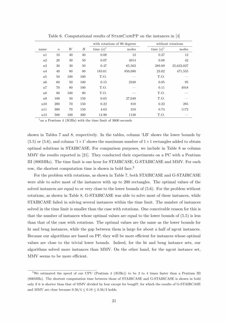
Table 6. Computational results of StairCasePP on the instances in [4]

with rotations of 90 degrees without rotations

name n W H time (s)† nodes time (s)† nodes

n1 10 40 40 0.08 12 0.27 12

n2 20 30 50 0.07 4014 0.08 42

n3 30 30 50 0.47 65,562 289.09 25,633,027

n4 40 80 80 183.61 850,080 23.02 471,555

n5 50 100 100 T.O. — T.O. —

n6 60 50 100 0.15 2348 0.05 95

n7 70 80 100 T.O. — 0.11 4918

n8 80 100 80 T.O. — T.O. —

n9 100 50 150 0.65 27,049 T.O. —

n10 200 70 150 0.22 818 0.22 285

n11 300 70 150 4.63 318 0.74 1172

n12 500 100 300 14.90 1138 T.O. —†on a Pentium 4 (3GHz) with the time limit of 3600 seconds

shown in Tables 7 and 8, respectively. In the tables, column ‘LB’ shows the lower bounds by

(5.5) or (5.6), and column ‘1×1’ shows the maximum number of 1×1 rectangles added to obtain

optimal solutions in STAIRCASE. For comparison purposes, we include in Table 8 as column

MMV the results reported in [21]. They conducted their experiments on a PC with a Pentium

III (800MHz). The time limit is one hour for STAIRCASE, G-STAIRCASE and MMV. For each

row, the shortest computation time is shown in bold face.5

For the problem with rotations, as shown in Table 7, both STAIRCASE and G-STAIRCASE

were able to solve most of the instances with up to 200 rectangles. The optimal values of the

solved instances are equal to or very close to the lower bounds of (5.6). For the problem without

rotations, as shown in Table 8, G-STAIRCASE was able to solve most of these instances, while

STAIRCASE failed in solving several instances within the time limit. The number of instances

solved in the time limit is smaller than the case with rotations. One conceivable reason for this is

that the number of instances whose optimal values are equal to the lower bounds of (5.5) is less

than that of the case with rotations. The optimal values are the same as the lower bounds for

ht and beng instances, while the gap between them is large for about a half of ngcut instances.

Because our algorithms are based on PP, they will be more efficient for instances whose optimal

values are close to the trivial lower bounds. Indeed, for the ht and beng instance sets, our

algorithms solved more instances than MMV. On the other hand, for the ngcut instance set,

MMV seems to be more efficient.

5We estimated the speed of our CPU (Pentium 4 (3GHz)) to be 3 to 4 times faster than a Pentium III

(800MHz). The shortest computation time between those of STAIRCASE and G-STAIRCASE is shown in bold

only if it is shorter than that of MMV divided by four except for beng07, for which the results of G-STAIRCASE

and MMV are close because 0.56/4 ≤ 0.18 ≤ 0.56/3 holds.

21

Table 7. Computational results on 2SP (with rotations of 90 degrees)

STAIRCASE G-STAIRCASE

name n W LB H∗ 1 × 1 time (s)† nodes time (s)† nodes

ht01 16 20 20 20 0 0.10 204 0.07 204

ht02 17 20 20 20 0 0.07 253 0.10 253

ht03 16 20 20 20 0 0.08 26 0.05 26

ht04 25 40 15 15 0 0.10 2,356 0.12 2,358

ht05 25 40 15 15 0 0.09 196 0.09 204

ht06 25 40 15 15 0 0.11 7,607 0.11 7,563

ht07 28 60 30 30 0 0.09 36 0.13 36

ht08 29 60 30 30 0 0.19 8,245 0.14 8,238

ht09 28 60 30 30 0 0.09 484 0.10 484

beng01 20 25 30 30 9 0.08 54 0.08 55

beng02 40 25 57 57 5 0.12 94 0.10 100

beng03 60 25 84 84 10 0.10 125 0.10 310

beng04 80 25 107 107 2 0.08 369 0.13 370

beng05 100 25 134 134 20 0.08 185 0.13 198

beng06 40 40 36 36 20 0.10 69 0.12 684

beng07 80 40 67 67 7 0.11 91 0.11 87

beng08 120 40 101 101 13 0.17 1,045 0.18 1,027

beng09 160 40 126 126 32 0.23 194 0.41 14,332

beng10 200 40 156 156 23 0.81 325 3.53 80,505

cgcut01 16 10 23 23 5 0.16 29 0.10 107

cgcut02 23 70 63 63 66 0.18 13,132 0.75 84,064

cgcut03 62 70 636 — T.O. — T.O. —

ngcut01 10 10 19 20 10 0.35 3,367 0.14 2715

ngcut02 17 10 28 28 3 0.11 536 0.14 41

ngcut03 21 10 28 28 3 0.11 939 0.11 79

ngcut04 7 10 17 18 18 0.29 40,664 0.15 581

ngcut05 14 10 36 36 7 0.08 2,068 0.08 2,390

ngcut06 15 10 29 29 0 0.09 1,632 0.06 1,628

ngcut07 8 20 9 10 25 0.39 82,772 0.13 1,739

ngcut08 13 20 32 33 27 917.96 72,350,616 8.80 946,103

ngcut09 18 20 49 49 6 0.11 2,798 0.10 1,779

ngcut10 13 30 58 59 50 T.O. — 2.28 273,329

ngcut11 15 30 50 — T.O. — T.O. —

ngcut12 22 30 77 77 14 8.54 978,092 12.66 935,604†on a Pentium 4 (3GHz) with the time limit of 3600 seconds

22

Table 8. Computational results on 2SP (without rotations)

STAIRCASE G-STAIRCASE MMV

name n W LB H∗ 1 × 1 time (s)† nodes time (s)† nodes time (s)‡

ht01 16 20 20 20 0 0.10 52 0.07 52 10.84

ht02 17 20 20 20 0 0.12 1,325 0.07 1,315 623.53

ht03 16 20 20 20 0 0.08 22 0.10 22 500.75

ht04 25 40 15 15 0 0.08 3,547 0.11 3,545 8.26

ht05 25 40 15 15 0 0.09 599 0.06 599 20.29

ht06 25 40 15 15 0 0.11 2,215 0.06 2,212 16.94

ht07 28 60 30 30 0 0.12 1,340 0.10 1,340 T.O.

ht08 29 60 30 30 0 71.40 3,030,967 76.97 2,957,065 T.O.

ht09 28 60 30 30 0 0.10 116 0.13 116 0.00

beng01 20 25 30 30 9 0.53 74,209 0.93 95,784 511.58

beng02 40 25 57 57 5 1.13 94,169 22.89 463,205 T.O.

beng03 60 25 84 84 10 0.94 40,653 0.32 10,311 T.O.

beng04 80 25 107 107 2 0.25 5,309 T.O. — T.O.

beng05 100 25 134 134 20 0.15 4,345 0.31 8,530 500.62

beng06 40 40 36 36 20 0.07 204 0.29 25,369 T.O.

beng07 80 40 67 67 7 0.33 9,021 0.18 802 0.56

beng08 120 40 101 101 13 1.36 33,596 2.67 77,150 500.54

beng09 160 40 126 126 32 0.42 7,047 2.38 39,467 0.03

beng10 200 40 156 156 23 2.86 6,977 6.52 101,671 0.03

cgcut01 16 10 23 23 5 0.10 3,789 0.12 3,578 11.48

cgcut02 23 70 63 — T.O. — T.O. — T.O.

cgcut03 62 70 636 — T.O. — T.O. — T.O.

ngcut01 10 10 19 23 40 2080.04 257,058,531 0.39 23,854 0.05

ngcut02 17 10 28 30 13 T.O. — T.O. — 11.31

ngcut03 21 10 28 28 3 0.09 184 0.10 152 27.01

ngcut04 7 10 17 20 38 3.63 766,572 0.14 106 0.00

ngcut05 14 10 36 36 7 0.11 56 0.07 83 0.00

ngcut06 15 10 29 31 20 T.O. — 147.31 4,423,772 727.20

ngcut07 8 20 20 20 225 T.O. — 0.10 16 0.00

ngcut08 13 20 32 33 27 30.51 3,911,039 0.50 39,291 53.09

ngcut09 18 20 49 50 26 T.O. — 1971.64 42,196,600 T.O.

ngcut10 13 30 58 80 680 T.O. — 113.98 12,642,065 0.18

ngcut11 15 30 50 52 77 T.O. — 7.71 573,883 483.01

ngcut12 22 30 77 87 314 T.O. — T.O. — 0.00†on a Pentium 4 (3GHz) with the time limit of 3600 seconds‡on a Pentium III (800MHz) with the time limit of 3600 seconds

23

7 Branch-and-bound algorithm based on sequence pairs

We examined another branch-and-bound algorithm based on a different scheme for representing

solutions. It is based on the sequence pair representation proposed in [25], which defines relative

positions of rectangles by using a pair of permutations of the set I. An interesting feature of this

scheme is that polynomial-time algorithms for encoding and decoding are known [11, 25], where

encoding is to find the sequence pair representation that does not contradict a given placement,

while decoding is to find the best placement among those that satisfy the constraints on the

relative positions of rectangles defined by a given sequence pair.

One of the merits of this branch-and-bound algorithm is that it can handle instances having

non-integer values for widths and heights, while the algorithms proposed in Sections 4 and 5

and those in [17, 21] require that all input values are integers.

Our algorithm based on sequence pairs could solve instances with up to 10 (resp., 11) rect-

angles for the case with (resp., without) rotations within the time limit of two hours on a PC

with a Pentium 4 (3GHz). However, these results are not competitive with those reported in

Section 6. We therefore omit the details of this algorithm in this paper. The description of this

algorithm and its computational results are reported in [16].

8 Conclusions

We proposed several ideas for exactly solving the perfect packing (PP) and strip packing (2SP)

problems using the branch-and-bound method. We confirmed through computational experi-

ments that branching based on the staircase placement is effective for PP. Our algorithm based

on this idea was able to solve all the benchmark instances with up to 29 rectangles for the case

with rotations of 90 degrees and was able to solve all but one instance with up to 49 rectangles

for the case without rotations. Moreover, it succeeded in solving several benchmark instances

with up to 500 rectangles in less than 15 seconds. We also observed that our algorithms for

2SP were efficient for instances whose optimal values are close to the trivial lower bounds; they

solved most of the benchmark instances with up to 200 rectangles within one hour. For the

case without rotations, one of our algorithms for PP outperformed the algorithm in [17], and

our algorithms for 2SP were competitive with the method in [21]. Considering the fact that the

existing algorithms are tailored for the case without rotations, these results are quite satisfactory.

Acknowledgment

The authors would like to thank Shinji Imahori and anonymous referees for valuable comments.

This research was supported by a Scientific Grant-in-Aid by the Ministry of Education, Culture,

Sports, Science and Technology of Japan.

24

References

[1] Alvarez-Valdes R, Parreno F, Tamarit JM. Reactive GRASP for the Strip-Packing Problem.

Computers and Operations Research; 2008; 35; 1065–1083.

[2] Baker BS, Coffman Jr. EG, Rivest RL. Orthogonal Packings in Two Dimensions. SIAM

Journal on Computing 1980; 9; 846–855.

[3] Bortfeldt A. A Genetic Algorithm for the Two-Dimensional Strip Packing Problem with

Rectangular Pieces. European Journal of Operational Research 2006; 172; 814–837.

[4] Burke EK, Kendall G, Whitwell G. A New Placement Heuristic for the Orthogonal Stock-

Cutting Problem. Operations Research 2004; 52; 655–671.

[5] Chazelle B. The Bottom-Left Bin-Packing Heuristic: An Efficient Implementation. IEEE

Transactions on Computers 1983; C-32; 697–707.

[6] Dowsland KA. Some Experiments with Simulated Annealing Techniques for Packing Prob-

lems. European Journal of Operational Research 1993; 68; 389–399.

[7] Hopper E, Turton BCH. An Empirical Investigation of Meta-Heuristic and Heuristic Algo-

rithms for a 2D Packing Problem. European Journal of Operational Research 2001; 128;

34–57.

[8] Hopper E, Turton BCH. A Review of the Application of Meta-Heuristic Algorithms to 2D

Strip Packing Problems. Artificial Intelligence Review 2001; 16; 257–300.

[9] Huang W, Chen D. An Efficient Heuristic Algorithm for Rectangle-Packing Problem. Sim-

ulation Modelling Practice and Theory 2007; 15; 1356–1365.

[10] Ibaraki T. Enumerative Approaches to Combinatorial Optimization. Annals of Operations

Research, vols.10 and 11; JC Baltzer AG; Basel; 1987.

[11] Imahori S, Yagiura M, Ibaraki T. Local Search Algorithms for the Rectangle Packing Prob-

lem with General Spatial Costs. Mathematical Programming 2003; Series B 97; 543–569.

[12] Imahori S, Yagiura M, Ibaraki T. Improved Local Search Algorithms for the Rectangle

Packing Problem with General Spatial Costs. European Journal of Operational Research

2005; 167; 48–67.

[13] Imahori S, Yagiura M, Nagamochi H. Practical Algorithms for Two-Dimensional Packing.

In: Gonzalez TF (ed), Handbook of Approximation Algorithms and Metaheuristics. Chap-

man & Hall/CRC in the Computer & Information Science Series; 2007. Chapter 36.

[14] Iori M, Martello S, Monaci M. Metaheuristic Algorithms for the Strip Packing Problem.

In: Pardalos PM, Korotkikh V (eds), Optimization and Industry: New Frontiers. Kluwer

Academic Publishers: Dordrecht, The Netherlands; 2003. p. 159–179.

[15] Jakobs S. On Genetic Algorithms for the Packing of Polygons. European Journal of Oper-

ational Research 1996; 88; 165–181.

[16] Kenmochi M, Imamichi T, Nonobe K, Yagiura M, Nagamochi H. Exact Algorithms for the

2-Dimensional Strip Packing Problem with and without Rotations. Technical Report 2007-

005, Department of Applied Mathematics and Physics, Graduate School of Informatics,

25

Kyoto University, January, 2007 (available at http://www.amp.i.kyoto-u.ac.jp/tecrep/).

[17] Lesh N, Marks J, McMahon A, Mitzenmacher M. Exhaustive Approaches to 2D Rectangular

Perfect Packings. Information Processing Letters 2004; 90; 7–14.

[18] Lesh N, Marks J, McMahon A, Mitzenmacher M. New Heuristic and Interactive Approaches

to 2D Rectangular Strip Packing. ACM Journal of Experimental Algorithmics 2005; 10; 1–

18.

[19] Liu D, Teng H. An Improved BL-Algorithm for Genetic Algorithm of the Orthogonal Pack-

ing of Rectangles. European Journal of Operational Research 1999; 112; 413–420.

[20] Lodi A, Martello S, Monaci M. Two-Dimensional Packing Problems: A Survey. European

Journal of Operational Research 2002; 141; 241–252.

[21] Martello S, Monaci M, Vigo D. An Exact Approach to the Strip-Packing Problem.

INFORMS Journal on Computing 2003; 15; 310–319.

[22] Martello S, Pisinger D, Vigo D. The Three-Dimensional Bin Packing Problem. Operations

Research 2000; 48; 256–267.

[23] Martello S, Toth P. Knapsack Problems—Algorithms and Computer Implementations. John

Wiley & Sons: Chichester; 1990.

[24] Matsuda Y. The Fourth Supercomputer Programming Contest for High School Students

at Tokyo Institute of Technology. Sugaku Seminar (Mathematics Seminar) 1998; 37(12);

40–43, in Japanese.

[25] Murata H, Fujiyoshi K, Nakatate S, Kajitani Y. VLSI Module Placement Based on

Rectangle-Packing by the Sequence-Pair. IEEE Transactions on Computer-Aided Design

of Integrated Circuits and Systems 1996; 15; 1518–1524.

[26] Turek J, Wolf JL, Yu PS. Approximate Algorithms for Scheduling Parallelizable Tasks. Pro-

ceedings of the Fourth Annual ACM Symposium on Parallel Algorithms and Architectures

1992; 323–332.

[27] Wascher G, Haußner H, Schumann H, An Improved Typology of Cutting and Packing

Problems, European Journal of Operational Research 2007; 183; 1109–1130.

[28] Wei L, Zhang D, Chen Q. A Least Wasted First Heuristic Algorithm for the Rectangular

Packing Problem. Computers and Operations Research; to appear.

[29] Yeung LHW, Tang WKS. Strip-Packing Using Hybrid Genetic Approach. Engineering Ap-

plications of Artificial Intelligence 2004; 17; 169–177.

[30] Zhang DF, Chen SD, Liu YJ. An Improved Heuristic Recursive Strategy Based on Genetic

Algorithm for the Strip Rectangular Packing Problem. Acta Automatica Sinica 2007; 33;

911–916.

[31] Zhang D, Kang Y, Deng A. A New Heuristic Recursive Algorithm for the Strip Rectangular

Packing Problem. Computers and Operations Research 2006; 33; 2209–2217.

26