Algorithms for Molecular Biology F all Semester, 1998rshamir/algmb/98/scribe/pdf/lec12.pdf · Algorithms for Molecular Biology F all Semester, 1998 ... the DNA molecule is comp osed

Algorithms for Molecular Biology Fall Semester, 1998

Lecture 12: February 21, 1999

Lecturer: Ron Shamir Scribe: Dror Irony and David Oren

In this document we will brie y discuss several topics:

1. Hybridization

2. cDNA clustering

3. Analyzing gene expression data

These topics will be addressed very brie y. The interested reader is referred to the

bibliography for more details on these subjects.

12.1 Hybridization

12.1.1 What is Hybridization?

As we have already seen, under normal conditions, the DNA molecule is composed of two

strands. These two strands are connected by hydrogen bonds, and together form the well-

known double helix structure.

When a solution containing DNA is heated, these hydrogen bonds disappear, and the

two strands drift apart. This single-stranded DNA is called denatured DNA (or, surprisingly

enough single-stranded DNA). When the solution is cooled, hydrogen bonds form between

matching bases in the strands. These bonds are formed in places where a match (or at least

a partial match) exists. If these bonds begin to form in corresponding parts of two strands,

they will quickly completely join and the double-helix will reappear. However, this is not

guaranteed to happen. Bonds can form even between strands of di�erent DNA molecules or

strands of di�erent length.

Let us take short single-stranded chains of nucleotides, called oligonucleotides (or oligos

for short), that we have synthesized and add them to the heated DNA solution. Each oligo is

a known nucleotide sequence between 10 and 12 bases long. Now, when the solution is cooled,

the oligos will stick to parts of the DNA which contain a DNA sequence complementary to

that of the oligo. The resulting composition is called hybrid DNA.

12.1.2 Motivation

Many biological techniques are based on hybridization. For instance, consider the following

situation: Let us take human DNA and oligos obtained from coding regions of mouse DNA

1

2 Shamir: Algorithms for Molecular Biology c Tel Aviv Univ., Fall '98

(each one several hundred bases long). Let us now create a hybrid of the two. Since homology

between these DNAs exists mostly in the coding regions, we can use the hybridization to

infer where human coding regions are. If the oligos are tagged, either with uorescent dye or

radioactive label, one can detect where the oligos hybridized with the DNA, and thus infer

what the coding regions are (or at least, which regions deserve further study).

12.1.3 DNA Chips

Hybridization experiments were traditionally performed using page-sized �lters, with each

�lter having about 10 bands displaying whether hybridization occurred or not.

About ten years ago the techniques became developed enough to allow miniaturized

�lters, which are chip sized, with each band being about 100 microns wide. Using these

DNA chips, also called DNA arrays, also enables us to perform several experiments at once.

There are two types of DNA chips. Both share the same basic idea, but the implementa-

tion is di�erent in each. We will discuss these chip types in the order they were introduced.

Type I chips

This type of chips was the �rst to be used. These chips consist of a matrix, with each cell of

the matrix containing one target DNA. The chip is exposed to a solution containing many

identical oligos, and hybridization occurs between matching DNA and oligos. Again, if the

oligos are tagged, either with uorescent dye or radioactive label, we can then see at each

point of the matrix whether the hybridization occurred (i.e., which of the DNAs hybridized

with the oligo we tested).

The chip can then be heated, separating the oligos from the DNA, and the experiment

can be repeated with a di�erent type of oligo.

Finally, we get a matrix M , with each row representing a speci�c target DNA from the

matrix, and each column representing an oligo:

Mi;j =

8<:1 if hybridization occurred between DNA i and oligo j

0 no hybridization occurred

The chips contain some 50,000 cells of target DNA and the experiment can be repeated

with 100 to 500 oligos. The advantage of using a DNA chip is obvious: each experiment

tests an oligo against 50,000 target DNA at once.

In 1989, six patent applications were issued for this kind of DNA chips, and the issue is

still debated in court. However, nowadays most people use di�erent chips.

Hybridization 3

Type II chips

The basic idea in these chips is similar. The di�erence is that these chips contain the oligos,

and not the targets. The length of the oligos used depends on the application, but they are

usually no longer than 25 bases. Since oligos are usually shorter, the density is much higher

in these chips. For instance, a chip that is 1cm by 1cm can easily contain 100,000 oligos.

The chips are used in a similar manner. They are exposed to a solution containing many

copies of the target DNA. Hybridization occurs between oligos and matching DNA and then

the chip can be heated in order to repeat the experiment.

While the basic idea is the same, the chips are obviously intended for di�erent experi-

ments. The second kind of chips is most useful in situation where we have relatively few

targets, but a large number of oligos we wish to test. Another advantage is that we may

want to hybridize targets against a \standard" oligo library. The oligo chips can thus be

manufactured in large quantities, and their cost decreases.

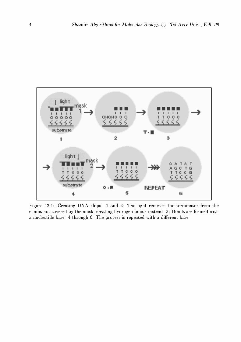
Manufacturing chips

DNA chips are produced in a way that is similar to the way computer chips are. We start

with a matrix created over a glass substrate. Each cell in the matrix contains a \chain"

with appropriate chemical properties, and ending with a terminator, a chemical gadget that

prevents chain extension.

We cover this substrate with a mask, covering some of the cells, but not others. We

can then illuminate the substrate. Covered cells are una�ected. In cells that are hit by the

light, the bond with the terminator is severed. If we now expose the substrate to a solution

containing a nucleotide base, it will form bonds with the non-terminated chains. Thus, some

of the cells will now contain this nucleotide.

The process can then be repeated with di�erent masks, and for di�erent nucleotides. This

way we can insert a speci�c nucleotide to each cell of the matrix. Figure 12.1 demonstrates

the production process.

It should be mentioned that in practice the process is much more complicated than that.

For instance, di�raction can be a problem near the edge of the substrate, and we cannot be

sure that the chain binds to the nucleotide that is present in the solution. Another problem

is the manufacturing of the masks, which tends to be rather expensive (of course, these costs

are amortized for standard chips, but specialized chips are still expensive).

12.1.4 Sequencing by Hybridization

Standard oligo chips can, at least theoretically, be used for sequencing. Let us prepare an

oligo chip that contains all possible sequences of length k. These sequences are called k-mers.

Practical values of k are 8-10. If we expose this chip to a solution containing some target


Figure 12.1: Creating DNA chips. 1 and 2: The light removes the terminator from the

chains not covered by the mask, creating hydrogen bonds instead. 3: Bonds are formed with

a nucleotide base. 4 through 6: The process is repeated with a di�erent base.

Hybridization 5

DNA, the results will show which k-mers occur in the target sequence. This gives rise to the

de�nition of the k-spectrum of a sequence T as the multi-set of all its substrings of length k.

We would now like to reconstruct this sequence.

Problem 12.1 Reconstructing a sequence from hybridization data

INPUT: A multi-set S of k-mers

QUESTION: Is S the spectrum of a sequence T? If yes, reconstruct this sequence.

It should be noted that we assume that if a k-mer appears several times in the target

DNA, the hybridization experiment will report its multiplicity (this is why we require the

input to be a multi-set and not simply a set). To date, this requirement is impractical.

For instance, for k = 3:

T = ATGCAGGTCCAG

S = fATG;AGG;CAG;GCA;GGT;GTC; TCC; TGC;CCA;CAGg

The naive approach

Let us de�ne a directed graph G = (V;E), where V = fexisting k-mersg and an edge

e = (v1; v2) exists i� the last k � 1 characters of v1 match the �rst k � 1 characters of v2.

For instance, in our previous example, there will be an edge from ATG to TGC.

The problem is now to �nd a Hamiltonian path in the directed graph G. However, as

we should all be aware, the traveling salesman problem is NP-hard. Therefore, this solution

cannot be used for large input sets. While approximations and heuristics for the TSP exist,

no true computer scientist will be satis�ed with this solution.

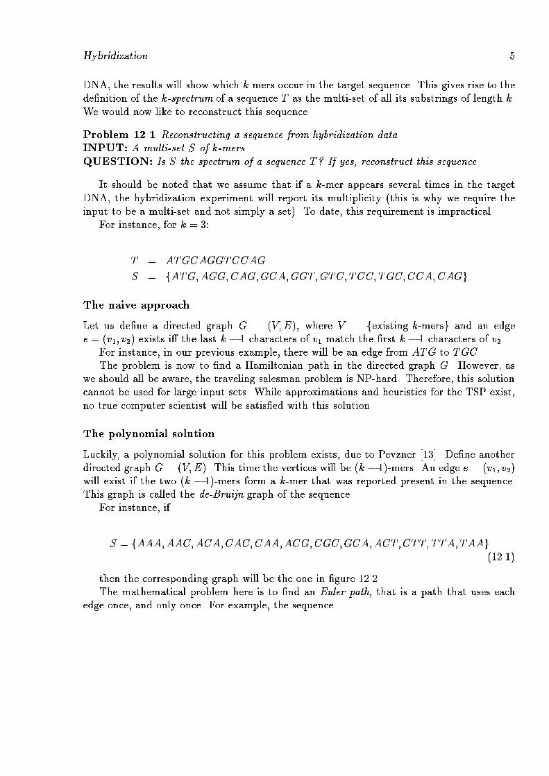
The polynomial solution

Luckily, a polynomial solution for this problem exists, due to Pevzner [13]. De�ne another

directed graph G = (V;E). This time the vertices will be (k � 1)-mers. An edge e = (v1; v2)

will exist if the two (k � 1)-mers form a k-mer that was reported present in the sequence.

This graph is called the de-Bruijn graph of the sequence.

For instance, if

S = fAAA;AAC;ACA;CAC;CAA;ACG;CGC;GCA;ACT;CTT; TTA; TAAg(12.1)

then the corresponding graph will be the one in �gure 12.2.

The mathematical problem here is to �nd an Euler path, that is a path that uses each

edge once, and only once. For example, the sequence


Figure 12.2: The (k�1)-mer graph constructed given the k-spectrum (k = 3) in equation 12.1

T = ACAAACGCACTTAA

is a solution to the instance whose graph is depicted in �gure 12.2, corresponding to the

Euler path

AC ! CA! AA! AA! AC ! CG! GC ! CA! AC ! CT ! TT ! TA! AA

in that graph. It should be noted that for this construction, it is very important to know

whether a given k-mer occurs more than once in the target sequence. For instance, if ACA

occurs two times in S, then there should be two edges between AC and CA. Otherwise, our

solution will not be correct.

While this solution is mathematically elegant, there are several problems with using it in

true biological context:

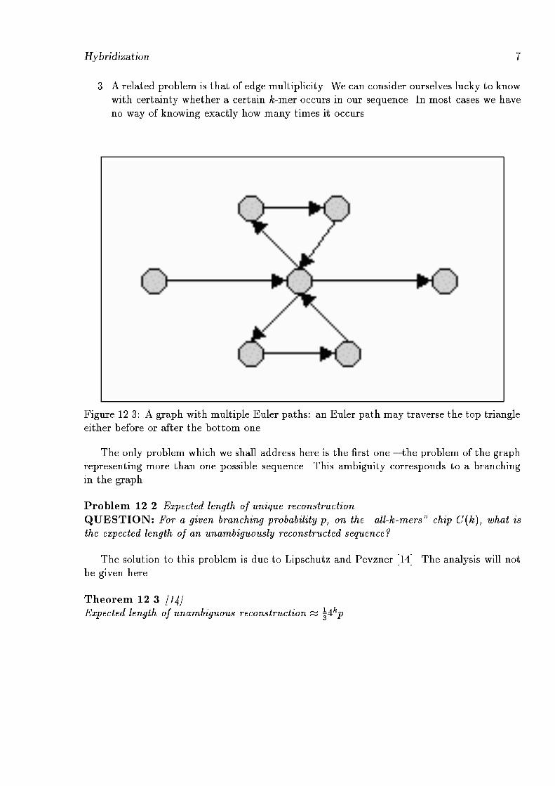
1. For some graph con�gurations, there is more than once Euler path. In such cases we

will not be able to reconstruct the sequence. For an example of such a graph, see

�gure 12.3.

2. As in all biological experiments, the spectrum we measure contains a large proportion

of errors. This solution is not robust enough to handle them.

Hybridization 7

3. A related problem is that of edge multiplicity. We can consider ourselves lucky to know

with certainty whether a certain k-mer occurs in our sequence. In most cases we have

no way of knowing exactly how many times it occurs.

Figure 12.3: A graph with multiple Euler paths: an Euler path may traverse the top triangle

either before or after the bottom one.

The only problem which we shall address here is the �rst one { the problem of the graph

representing more than one possible sequence. This ambiguity corresponds to a branching

in the graph.

Problem 12.2 Expected length of unique reconstruction

QUESTION: For a given branching probability p, on the \all-k-mers" chip C(k), what is

the expected length of an unambiguously reconstructed sequence?

The solution to this problem is due to Lipschutz and Pevzner [14]. The analysis will not

be given here.

Theorem 12.3 [14]

Expected length of unambiguous reconstruction � 1

34kp


If we take k = 8, which is a practical length, and p = 0:01, we get that the expected

length of the reconstructed sequence is 210 bases. When one considers genes, that can be

several thousands of bases long, this is obviously not good enough.

Some other chip designs achieve a somewhat better result, but these designs are only

theoretical. They are usually very di�cult or impossible to manufacture, and cannot be

used in true biological context.

Sadly, then, sequencing based on hybridization is not a real alternative to standard

sequencing.

Other uses of hybridization

Hybridization has other uses in biology. We cannot discuss all of them, but we will mention

two more.

One of these uses is resequencing. If we have DNA that is already sequenced, we can

design a special purpose chip that will detect speci�c mutations in that DNA.

For instance, let us assume we have already sequenced the DNA of the HIV virus. We

can design a special-purpose chip, that will detect which type of the virus we are dealing

with. Detecting will be easy: Expose the chip to a solution containing virus DNA, and then

check where hybridization occurs. For each virus type, hybridization will occur with di�erent

oligos.

Similarly, hybridization can be used to detect Single Nucleotide Polymorphisms (SNPs),

that is point mutations in the DNA, common only to a part of the population.

12.2 cDNA Clustering

12.2.1 Motivation

As we have seen, genes a�ect the human body by being expressed, i.e., transcribed into

mRNA and translated into proteins that react with other molecules. It is therefore highly

interesting to analyze the expression pro�le of genes, i.e., in which tissues and at what stages

of development they are expressed. From this information we can sometimes guess what the

function of these genes is. This is especially true if we discover that the expression pro�le of

an unknown gene is similar to that of a known gene { usually, in such cases the functions of

these genes are related. Another important piece of information is the level of expression of

each gene. As we have seen before, di�erent genes have di�erent levels of expression { some

are translated into proteins more often than others.

With this in mind, we can know state our goal: to �nd which genes are expressed in each

tissue, and in what level.

This is easier said than done. An average tissue contains more than 10,000 expressed

genes, and their expression levels can vary by a factor of 10,000. Therefore, in order to be

cDNA Clustering 9

sure we �nd all the genes in a tissue, we should extract more than 105 transcripts per tissue.

Keeping in mind that there are about 100 di�erent types of tissue in the body, and that

we are interested in comparing di�erent growth stages (or disease stages), we can conclude

that we should analyze more than 107 transcripts. Obviously, we need cheap, e�cient and

large scale methods.

12.2.2 The Experimental Problem

Recall that a gene is transcribed into mRNA, which is then translated into a protein. In order

to check what genes are expressed in a given tissue, we use cDNA { a reverse-transcript of

the mRNA, which is more stable. There exists methods which enable us to extract cDNA in

large quantities from the tissue, and we can see, at a given moment, which cDNA molecules

exist in the tissue (details are omitted).

In fact, we sample cDNA molecules from the tissue. The more a gene is expressed, the

more samples of its matching cDNA we will �nd. The sample we have obtained contains

about 100,000 cDNA fragments, each of them between 500 and 2,500 base-pairs long, the

average being around 1,200.

Since the sampling was performed in the course of the transcription process, not all the

cDNA fragments we have from the same gene will be of the same length, but rather they

will all have a common endpoint (which is the starting point of the mRNA).

We can now formulate the problem we face:

Problem 12.4 Determining gene expression

INPUT: Unsequenced cDNA fragments from a tissue

GOAL: Find which genes are present, and in what abundance

The simple solution is to sequence all the cDNA fragments we have extracted from the

tissue. This is both wasteful and slow. We have extracted a very large quantity of cDNA,

and many fragments come from the same genes. Sequencing all of them will mean sequencing

the same genes over and over again.

12.2.3 The HCC Algorithm

Ideally, we would like to decide apriori which cDNAs come from the same gene, and sequence

only one representative of each family. The basic idea is therefore as follows:

1. Obtain a cheap and fast �ngerprint of each cDNA.

2. Use these �ngerprints to identify groups of cDNAs corresponding to the same gene.

3. Sequence only representatives from each group.


Note that as in all biological experiments, our measurements are a�ected by noise. In

order to deal with this noise, we sequence several representatives from each group.

Oligo �ngerprinting

This technique was developed by several researchers: Drmanac-Crkvenjakov [2], Bains-

Smith [3], Southern [17] and Macevics [8].

First, we create a type I DNA-array with the cDNAs we have extracted from the tissue.

We then perform a hybridization experiment against a short oligo (between 7 and 15 bases

long). We read the hybridization pattern, and we repeat this procedure with other oligos

(150-500 oligos are considered enough).

The result is a matrix M where Mij = 1 i� cDNA i hybridized with oligo j. For each

cDNA fragment i, the i-th row indicates which oligos hybridized to this fragment. Therefore,

we say that Mi is the �ngerprint of clone i. This �ngerprint, just like to a barcode, identi�es

the cDNA, and cDNA originating from the same gene will have a similar �ngerprint.

Clustering

Now that we have the �ngerprints of the di�erent cDNA, it remains to be seen how we can

sort them into groups that (hopefully) represent the same gene. For the speci�c problem

of clustering cDNA �ngerprints, several approaches were suggested previously. Drmanac

et al. [15] construct clusters according to connected components in the similarity graph.

However, even with a low false positives rate in the data, such an algorithm would incorrectly

merge true clusters. Meyer-Ewert, Mott and Lehrach [10] construct clusters according to

maximal cliques. This approach does not work well either, since computing all maximal

cliques is computationally di�cult. Moreover, a high false negative rate may break large

clusters into many maximal cliques, with a hard-to-detect overlap structure. Milosavljevic

et al. [12] construct clusters using a greedy algorithm. Like most greedy approaches, this

algorithm cannot well handle high noise levels, and the quality of its results is very sensitive

to the starting point.

The algorithm we will describe here is due to Shamir et al. [6].

Once again we will use graphs as our main tool. Let us de�ne a graph G = (V;E),

where the vertices are the extracted cDNA, and an edge e = (v1; v2) exists if v1 and v2 have

similar �ngerprints (for discussing the de�nition of similar �ngerprints, the interested reader

is referred to [6]).

Recall the following de�nitions:

1. The connectivity k(G) of a graph G is the minimum number of edges whose removal

results in a disconnected graph. If k(G) = l then G is said to be l-(edge)-connected.

cDNA Clustering 11

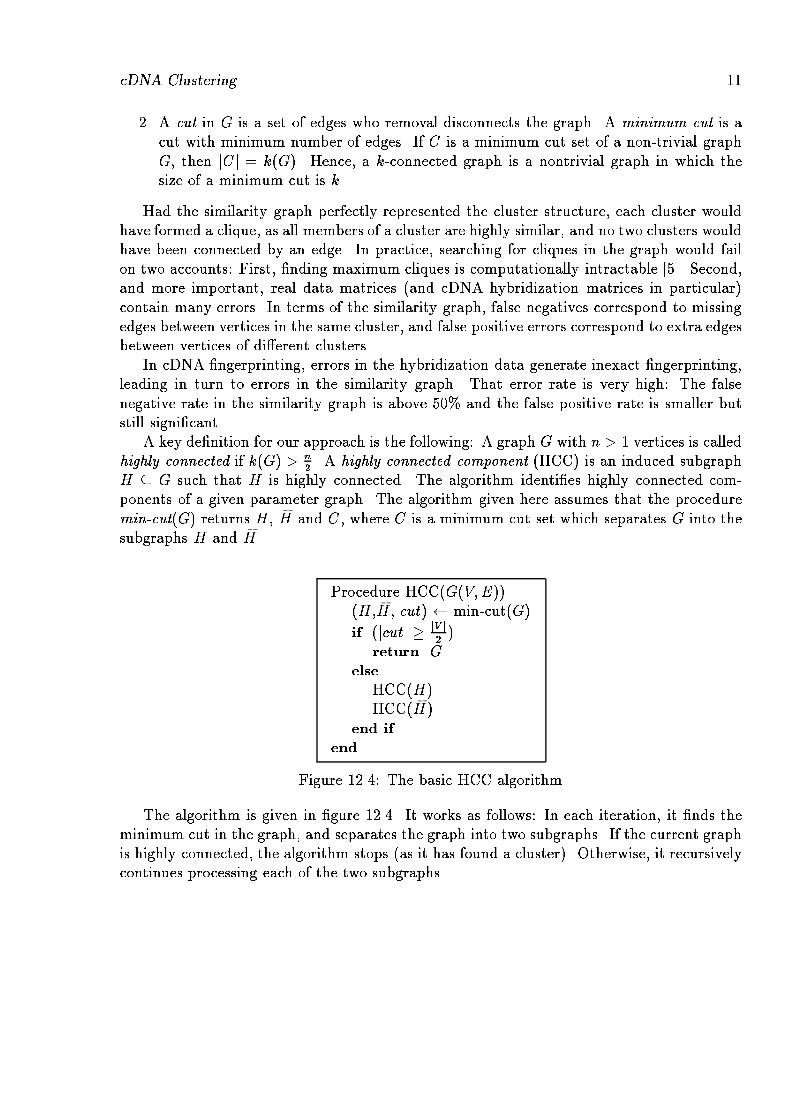
2. A cut in G is a set of edges who removal disconnects the graph. A minimum cut is a

cut with minimum number of edges. If C is a minimum cut set of a non-trivial graph

G, then jCj = k(G). Hence, a k-connected graph is a nontrivial graph in which the

size of a minimum cut is k.

Had the similarity graph perfectly represented the cluster structure, each cluster would

have formed a clique, as all members of a cluster are highly similar, and no two clusters would

have been connected by an edge. In practice, searching for cliques in the graph would fail

on two accounts: First, �nding maximum cliques is computationally intractable [5]. Second,

and more important, real data matrices (and cDNA hybridization matrices in particular)

contain many errors. In terms of the similarity graph, false negatives correspond to missing

edges between vertices in the same cluster, and false positive errors correspond to extra edges

between vertices of di�erent clusters.

In cDNA �ngerprinting, errors in the hybridization data generate inexact �ngerprinting,

leading in turn to errors in the similarity graph. That error rate is very high: The false

negative rate in the similarity graph is above 50% and the false positive rate is smaller but

still signi�cant.

A key de�nition for our approach is the following: A graph G with n > 1 vertices is called

highly connected if k(G) > n

2. A highly connected component (HCC) is an induced subgraph

H � G such that H is highly connected. The algorithm identi�es highly connected com-

ponents of a given parameter graph. The algorithm given here assumes that the procedure

min-cut(G) returns H, �H and C, where C is a minimum cut set which separates G into the

subgraphs H and �H.

Procedure HCC(G(V;E))

(H, �H, cut) min-cut(G)

if (jcutj � jV j2)

return G

else

HCC(H)

HCC( �H)

end if

end

Figure 12.4: The basic HCC algorithm

The algorithm is given in �gure 12.4. It works as follows: In each iteration, it �nds the

minimum cut in the graph, and separates the graph into two subgraphs. If the current graph

is highly connected, the algorithm stops (as it has found a cluster). Otherwise, it recursively

continues processing each of the two subgraphs.


Properties of HCC clustering

Theorem 12.5 The diameter of each cluster is smaller than or equal to 2. That is, the

distance between two vertices is at most 2.

Proof: Let k(G) be the size of the minimum cut, let d(v) denote the degree of v and

�(G) = minv d(v). Observe that k(G) � �(G): suppose to the contracy that d(v) < k(G)

for some v, then the cut (fvg; V n fvg) contradicts minimality of k(G). Furthermore, if G

is a cluster reported by the HCC algorithm, then according to the \if" statement in the

algorithm jV j2� k(G) (otherwise G would have been divided in two by HCC). Therefore,

�(G) > jV j2.

Consider two vertices v1 and v2 in G. If they are neighbors, then surely the theorem holds

for them. Let us therefore assume that they are not neighbors. From the previous inequality,

each one of these vertices has more than jV j2

neighbors in G. Therefore, they must have a

common neighbor, since the total number of vertices in the graph is jV j, and therefore the

total number of their neighbors cannot exceed jV j � 2.

While we have proven that each highly connected cluster has a small diameter, the

converse does not necessarily hold. That is, G may have a subgraph, with diameter 2 that

is not a highly connected component.

Lemma 12.6 Let S be a set of edges forming a minimum cut in the graph G = (V;E). Let

H and �H be the induced subgraphs obtained by removing S from G, where jV ( �H)j � jV (H)j.If jV ( �H)j > 1 then jSj � jV ( �H)j, with equality only if �H is a clique.

The lemma implies that if a minimum cut S in G = (V;E) satis�es jSj > jV j2then S splits

the graph into a single vertex fvg and Gnfvg. This shows us that using a stronger stopping

criterion for the algorithm, i.e., jSj > �, for � >jV j2

will be detrimental for clustering: Any

cut of value x > jV j2

separates only a singleton from the current graph.

Theorem 12.7 Let S be a minimum cut in the graph G = (V;E) where jSj � jV j2. Let H

and �H be the connected induced subgraphs obtained by removing S from G, where jV ( �H)j �jV (H)j. If diam(G) � 2 then (1) every vertex in �H is incident on S, (2) �H is a clique.

It can be shown, using this theorem, that the union of two vertex sets split by any step

of HCC is unlikely to induce a graph with diameter � 2 if noise is random, and the vertex

sets are not too small. Another property of the solution is given by:

Theorem 12.8 1. The number of edges in a highly connected subgraph is quadratic.

2. The number of edges removed by each iteration of the HCC algorithm is at most linear.

cDNA Clustering 13

Proof: Let n be the number of edges in the graph. Then:

1. As we have seen before, n2< k(G) � �(G). Since the rank of each vertex is > n

2, the

total number of edges is

N =1

2

Xv

�(v) >1

2

nXi=1

n

2=n2

4

2. The algorithm removes the edges forming the minimal cut S, only if jSj < n2. There-

fore, obviously the number of removed edges is linear.

12.2.4 Re�nements

The algorithm as was introduced can be re�ned using two heuristic methods:

Orphans Adoption

The basic HCC algorithm may leave certain vertices as unclustered singletons. For that

reason, each singleton is checked whether it has a lot of neighbors in one of the clusters.

If this is the case, the singleton is then added to that cluster. This improvement is called

orphans adoption.

The low degree heuristic

When the input graph contains low degree vertices, one iteration of a minimum cut algorithm

may simply separate a low degree vertex from the rest of the graph. This is computationally

very expensive, not informative in terms of clustering, and may happen many times if the

graph is large and sparse. Removing low degree vertices from the original graph before

running the HCC algorithm eliminates such iterations and signi�cantly reduces the running

time. The complete algorithm, after re�nements, is shown in �gure 12.5.

12.2.5 Assessing Clustering Quality

A measure for the quality of a solution given the true clustering should be devised. One can

describe a clustering of n elements by an n� n symmetric (0; 1) matrix C, where Cij = 1 i�

i and j belong the same cluster. Given matrix representations of the true clustering T and

any clustering C of the same data set, the Minkowski measure for the quality of C is the

normalized L2 distance between the two matrices

DM (T;C) =

qPi;j(Tij �Cij)2

kTk

An alternative is the all pairs measure:


Procedure HCC-LOOP(G(V;E))

for (i = 1 to p) do

H G

repeatedly remove all vertices of degree < di from H

until (no new cluster is found) do

HCC(H)

perform orphan adoption

remove clustered vertices from H

remove clustered vertices from G

end

Figure 12.5: Re�nements of the HCC algorithm. d1; d2; : : : ; dp is a decreasing sequence of

integers given as external input to the algorithm

Dap(T;C) =j f(i; j) j Tij = Cij = 1g j � j f(i; j) j Tij 6= Cijg j

j f(i; j) j Tij = 1g j

12.2.6 Simulation Results

Intensive tests of the algorithm on simulated data were performed. The simulation process

computes arti�cal gene �ngerprints (hybridized oligos) for each participating gene. For

each gene and a given �ngerprint, the precise locations along the gene are generated in a

realistic manner. Then, truncated clones of each gene are generated. Each clone inherits the

�ngerprints and their locations from its original gene (just the �ngerprints with locations

relevant to the clone's indices). Finally, each copy is incorporated with false positive and

false negative errors, again, realistically. If we denote the total number of oligos by p and

the total number of clones by N , then the result of the simulation is an N � p hybridizationmatrix H, where Hij = 1 if clone i hybridized with oligo j, and Hij = 0 otherwise.

The simulation results are summarized in �gure 12.6.

12.2.7 Clustering Real cDNA Data

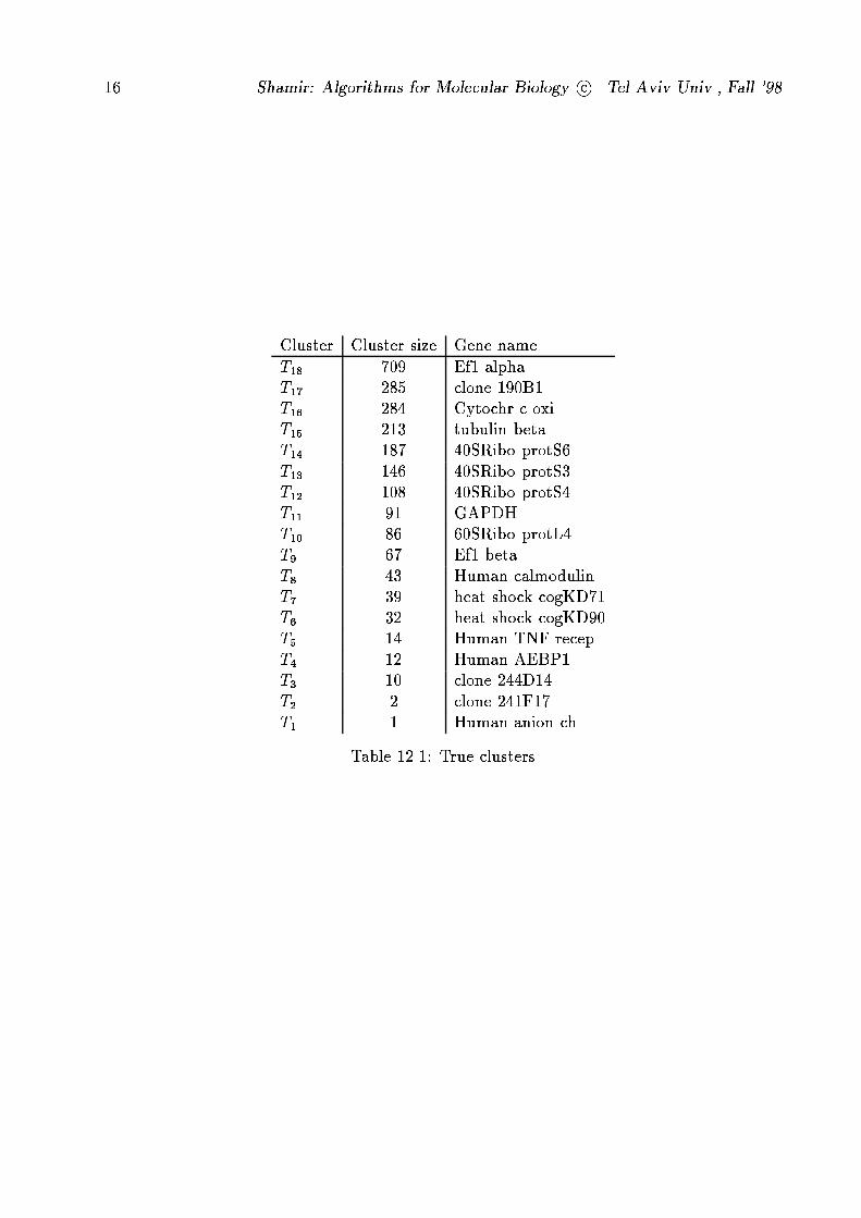
A test of clustering real cDNA data was performed. The input contained 2329 cDNAs,

originating from 18 genes. The true clustering, obtained by hybridization with long, unique

sequences, is given in table 12.1.

The high variability in abundance of genes can be easily seen. The results of the test are

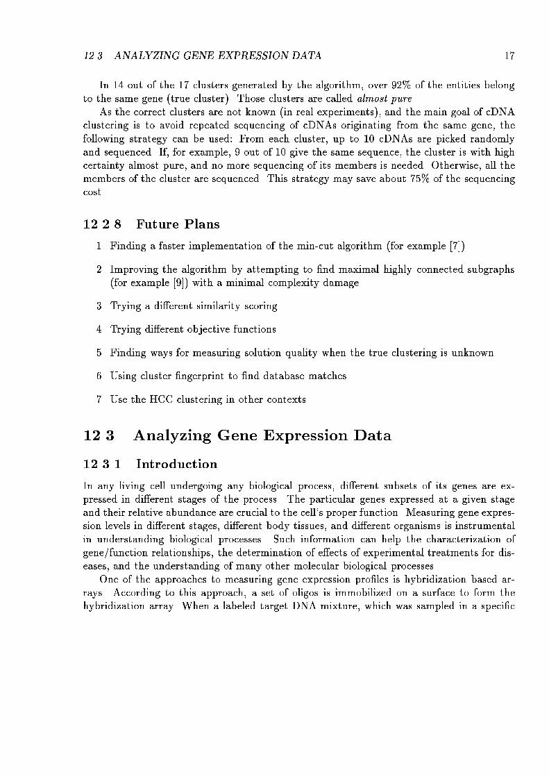
summarized in �gure 12.7.

cDNA Clustering 15

Figure 12.6: Examples of results of HCC and Greedy clustering algorithms in high noise

simulation. The �ngerprint data consisted of 780 cDNAs from 12 genes, in clusters of sizes

10,20,...,120. The number of oligos is 200. The expected rate of false positive hybridizations

is 25%. The expected false negative hybridization rate is 40%. A: The hybridization �nger-

prints matrix H. Each of the 780 rows is a �ngerprint vector of one cDNA. White denotes

positive hybridization. B: The binarized similarity matrix. Position i; j is black i� Sij > 50.

Matrix coordinates are scrambled, as in realistic scenarios. C: Clustering solution generated

by the greedy algorithm. Minkowski score is 1.32. cDNAs from the same true cluster appear

consecutively, and the black lines are the borders between the di�erent clusters. Position

i; j is black if the solution puts cDNAs i and j in the same cluster. D: Clustering solution

generated by the HCC algorithm. Minkowski score is 0.209.


Cluster Cluster size Gene name

T18 709 Ef1 alpha

T17 285 clone 190B1

T16 284 Cytochr c oxi

T15 213 tubulin beta

T14 187 40SRibo protS6



T11 91 GAPDH

T10 86 60SRibo protL4

T9 67 Ef1 beta

T8 43 Human calmodulin

T7 39 heat shock cogKD71

T6 32 heat shock cogKD90

T5 14 Human TNF recep

T4 12 Human AEBP1

T3 10 clone 244D14

T2 2 clone 241F17

T1 1 Human anion ch

Table 12.1: True clusters

12.3. ANALYZING GENE EXPRESSION DATA 17

In 14 out of the 17 clusters generated by the algorithm, over 92% of the entities belong

to the same gene (true cluster). Those clusters are called almost pure.

As the correct clusters are not known (in real experiments), and the main goal of cDNA

clustering is to avoid repeated sequencing of cDNAs originating from the same gene, the

following strategy can be used: From each cluster, up to 10 cDNAs are picked randomly

and sequenced. If, for example, 9 out of 10 give the same sequence, the cluster is with high

certainty almost pure, and no more sequencing of its members is needed. Otherwise, all the

members of the cluster are sequenced. This strategy may save about 75% of the sequencing

cost.

12.2.8 Future Plans

1. Finding a faster implementation of the min-cut algorithm (for example [7]).

2. Improving the algorithm by attempting to �nd maximal highly connected subgraphs

(for example [9]) with a minimal complexity damage.

3. Trying a di�erent similarity scoring.

4. Trying di�erent objective functions.

5. Finding ways for measuring solution quality when the true clustering is unknown.

6. Using cluster �ngerprint to �nd database matches.

7. Use the HCC clustering in other contexts.

12.3 Analyzing Gene Expression Data

12.3.1 Introduction

In any living cell undergoing any biological process, di�erent subsets of its genes are ex-

pressed in di�erent stages of the process. The particular genes expressed at a given stage

and their relative abundance are crucial to the cell's proper function. Measuring gene expres-

sion levels in di�erent stages, di�erent body tissues, and di�erent organisms is instrumental

in understanding biological processes. Such information can help the characterization of

gene/function relationships, the determination of e�ects of experimental treatments for dis-

eases, and the understanding of many other molecular biological processes.

One of the approaches to measuring gene expression pro�les is hybridization based ar-

rays. According to this approach, a set of oligos is immobilized on a surface to form the

hybridization array. When a labeled target DNA mixture, which was sampled in a speci�c


Figure 12.7: Clustering results on real cDNA data. A: The binarized similarity matrix. A

block point appears at position (i; j) i� Sij � 110. B: Reordering of A according to the true

clustering. cDNAs from the same t rue cluster appear consecutively, and the black lines are

the borders between the di�erent clusters. C: Reordering of A according to the clustering

produced by the HCC algorithm. Clusters appear in the order of detection. D: Comparison

of the algorithmic solution and the true solution. Rows and columns are ordered as in B.

Position (i; j) is black i� the algorithm put i and j in the same cluster.

Analyzing Gene Expression Data 19

condition (stage, tissue, organism, etc.), is introduced to the array, target sequences hybridize

to complementary immobilized molecules. The resulting hybridization intensity (detected,

for example, by uorescence) is indicative of the mixture's content and of the relative genes

expression measures in the tested condition. Di�erent conditions are tested, and eventually,

every gene has its own pro�le, i.e., vector of expression intensities, corresponding to the

di�erent conditions.

Clustering techniques are used to identify subsets of genes that behave similarly under the

set of tested conditions. Analyzing multi-conditional gene expresion patterns with clustering

algorithms involves the following steps:

1. Measuring gene expression levels, reported as a vector of real numbers.

2. Computing a similarity matrix for the genes (e.g., correlations).

3. Clustering the genes based on their similarity to each other.

4. Visual representation of the clusters.

5. Analysis of the results.

A speci�c clustering algorithm, CAST (for Cluster A�nity Search Technique) [18], which

is based on a graph theoretic approach, and uses a stochastic model of the input, was tried.

12.3.2 Temporal Gene Expression Patterns

In a previous study [11], the authors established some relationships between temporal gene

expression patterns of 112 rat CNS (Central Nervous System) genes and the development

process of the rat's CNS. Three major gene families were considered: Neuro-Glial Markers

family (NGMs), Neurotransmitter Receptors family (NTRs) and Peptide Signaling family

(PepS). All other genes measured in this study were lumped by the authors into a fourth

family: Diverse (Div). All families were further subdivided by the authors, based on apriori

biological knowledge. Gene expression patterns for the 112 genes of interest were measured

(using RT/PCR: [16]) in cervical spinal cord tissue, at nine di�erent developmental time

points. This yielded a 112�9 matrix of gene expression data. To capture the temporal nature

of this data, the authors transformed each (normalized) 9-dimensional expression vector into

a 17-dimensional vector, including also the 8 di�erence values between expression levels in

successive time points. This transformation emphasizes the similarity between genes with

closely parallel, but o�set, expression patterns. Euclidean distances between the augmented

vectors were computed, yielding a 112 � 112 distance matrix. Next, a phylogenetic tree

was constructed for this distance matrix (using the FITCH program [4]). Finally, cluster

boundaries were determined by visual inspection of the resulting tree. Some correlation

between the resulting clusters and the apriori family information was observed.


The CAST algorithm was tried on the same data in the following way: The raw expres-

sion data was preprocessed in a similar manner: �rst the normalized expression levels were

augmented with the derivative values. Then, a similarity matrix was computed based on

the L1 distance between the augmented 17-dimensional vectors. The CAST algorithm was

applied to the similarity matrix. Clusters were directly inferred (�gure 12.8).

12.3.3 Multi Experiment Analysis

Clustering gene expression patterns is useful even if the numbering of the experiments has no

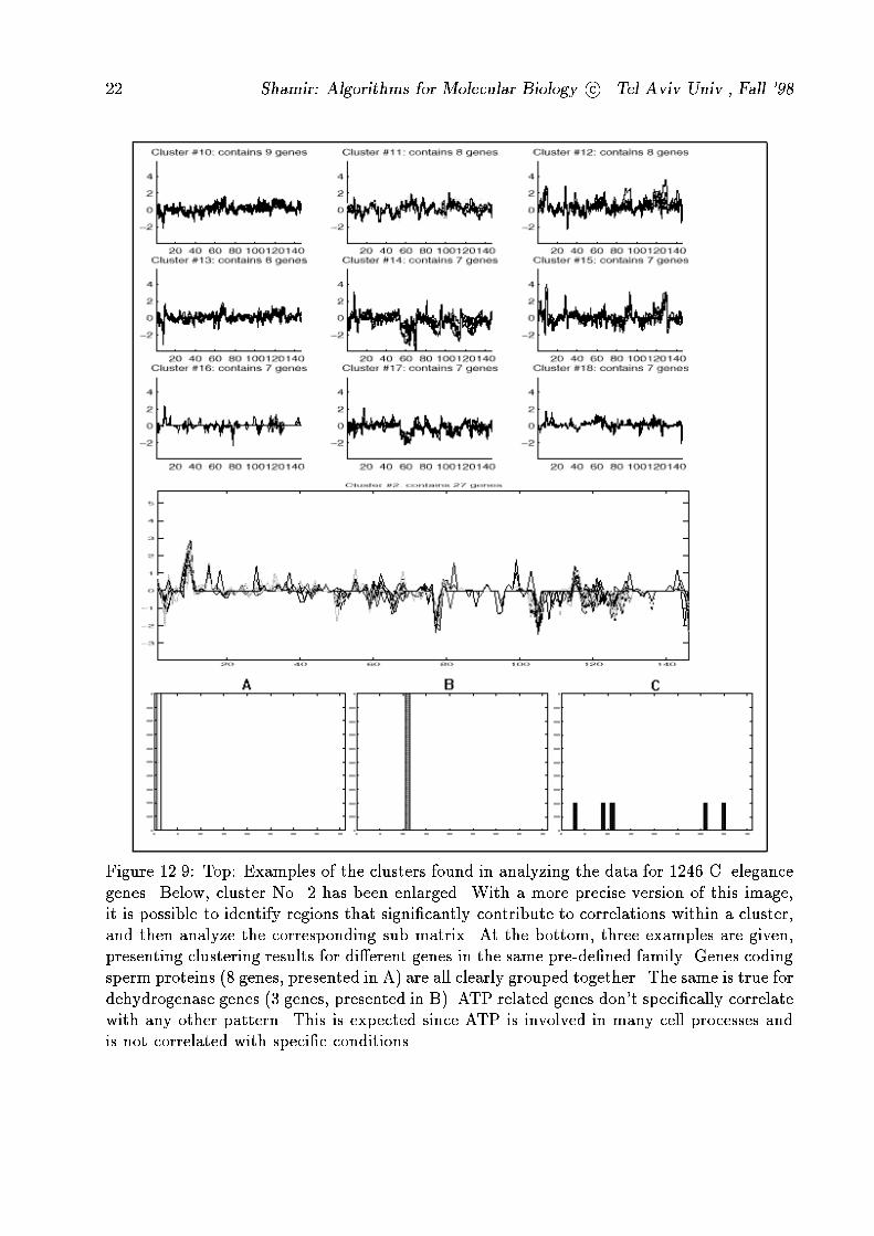
physical meaning (as opposed to temporal patterns). Using the CAST algorithm, data [1]

for 1246 C. elegance genes, from 146 experiments, was analyzed. The data was in the

form log(red/green) (representing the log-ratio of the two sample intensity values at the

corresponding array feature), per experiment. Contrary to the �rst trial, where the similarity

measure needed to re ect the temporal nature of the data, the order of experiments here, in

the total set, has little or no importance. Therefore, we use a unique similarity measure here.

Figure 12.9 summarizes the results. For temporal data it makes sense to use other similarity

measures when the corresponding sub matrices are clustered. Clustering the columns (rather

than the rows) of the expression matrix is also possible and contains biologically meaningful

information.

Analyzing Gene Expression Data 21

Figure 12.8: The unprocessed data is compared to the output of the clustering algorithm.

Top: The similarity matrix of the unprocessed data, compared against the new permutation

according to the found clusters. Bottom: The raw gene expression matrix is ordered accord-

ing to the permutation produced by the clustering algorithm and compared to the original

order.


Figure 12.9: Top: Examples of the clusters found in analyzing the data for 1246 C. elegance

genes. Below, cluster No. 2 has been enlarged. With a more precise version of this image,

it is possible to identify regions that signi�cantly contribute to correlations within a cluster,

and then analyze the corresponding sub matrix. At the bottom, three examples are given,

presenting clustering results for di�erent genes in the same pre-de�ned family. Genes coding

sperm proteins (8 genes, presented in A) are all clearly grouped together. The same is true for

dehydrogenase genes (3 genes, presented in B). ATP related genes don't speci�cally correlate

with any other pattern. This is expected since ATP is involved in many cell processes and

is not correlated with speci�c conditions.

Bibliography

[1] Stuart Kim's laboratory, Department of Developmental Biology, Stanford University,

http://cmgm.stanford.edu/ kimlab/.

[2] R. Drmanac amd R. Crkvenjakov, 1987. Yugoslav Patent Application 570.

[3] W. Bains and G. C. Smith. A novel method for nucleic acid sequence determination.

J. Theor. Biology, 135:303{307, 1988.

[4] J. Felsenstein. PHYLIP (Phylogeny Inference Package), version 3.5c, 1993. Distributed

by the author, Department of Genetics, University of Washington, Seattle.

[5] M. R. Garey and D. S. Johnson. Computers and Intractability: A Guide to the Theory

of NP-Completeness. W. H. Freeman and Co., San Francisco, 1979.

[6] E. Hartuv, A. Schmitt, J. Lange, S. Meier-Ewert, H. Lehrach, and R. Shamir. An

algorithm for clustering cDNAs for gene expression analysis using short oligonucleotide

�ngerprints. In Proceedings of the Human Genome Meeting, Torino, Italy, pages 27{28.

Nature Genetics, 1998.

[7] D.R. Karger. Minimum cuts in near linear time. In Proc. 28th annual ACM symposium

on theory of computing, pages 56{63, 1996.

[8] S. C. Macevics, 1989. International Patent Application PS US89 04741.

[9] D.W. Matula. k-Components, clusters and slicings in graphs. SIAM J. Appl. Math.,

22(3):459{480, 1972.

[10] S. Meier-Ewert, R. Mott, and H. Lehrach. Gene identi�cation by oligonucleotide �n-

gerprinting { a pilot study. Technical report, MPI, 1995.

[11] G. S. Michaels, D. B. Carr, M. Askenazi, S. Fuhrman, X. Wen, and R. Somogyi. Cluster

analysis and data visualization of large-scale gene expression data. In Proc. Paci�c

Symposium on Biocomputing, pages 42{53. World Scienti�c, 1998.

23

24 BIBLIOGRAPHY

[12] A. Milosavljevic, Z. Strezoska, M. Zeremski, D. Grujic, T. Paunesku, and R. Crkven-

jakov. Clone clustering by hybridization. Genomics, 27:83{89, 1995.

[13] P. A. Pevzner. l-tuple DNA sequencing: computer analysis. J. Biomol. Struct. Dyn.,

7:63{73, 1989.

[14] Pavel A. Pevzner and Robert J. Lipshutz. Towards DNA sequencing chips. In Igor

Pr��vara, Branislav Rovan, and Peter Ruzicka, editors, Mathematical Foundations of

Computer Science 1994 19th International Symposium, volume 841, pages 143{158,

Kosice, Slovakia, 22{26 August 1994. Springer.

[15] S. Drmanac N. A. Stavropoulos I. Labat J. Vonau B. Hauser M. B. Soares and R. Dr-

manac. Gene-representing cDNA clusters de�ned by hybridization of 57419 clones from

infant brain libraries with short oligonucleotide probes. Genomics, 37:29{40, 1996.

[16] R. Somogyi, X. Wen, W. Ma, and J. L. Barker. Developmental kinetics of GAD family

mRNAs parallel neurogenesis in the rat spinal cord. Journal of Neuroscience, 15:2575{

2591, 1995.

[17] E. Southern, 1988. UK Patent Application GB8810400.

[18] Z. Yakhini and A. Ben-Dor. Clustering gene expression patterns. Technical Report

HPL-98-190, HP-Labs Israel, 1998.

Documents

Algorithms for Molecular Biology F all Semester, 1998rshamir/algmb/98/scribe/pdf/lec12.pdf · Algorithms for Molecular Biology F all Semester, 1998 ... the DNA molecule is comp osed