CS222 Algorithms First Semester 2003/2004

CS222 AlgorithmsFirst Semester 2003/2004

Dr. Sanath JayasenaDept. of Computer Science & Eng.

University of Moratuwa

Lecture 7 (28/10/2003)String Matching Part 2

Greedy Approach

October 2003 Sanath Jayasena

7-2

Overview

• Previous lecture: String Matching Part 1– Naïve Algorithm, Rabin-Karp Algorithm

• This lecture– String Matching Part 2

• String Matching using Finite Automata• Knuth-Morris-Pratt (KMP) Algorithm

– Greedy Approach to Algorithm Design

String Matching

PART 2


7-4

Finite Automata

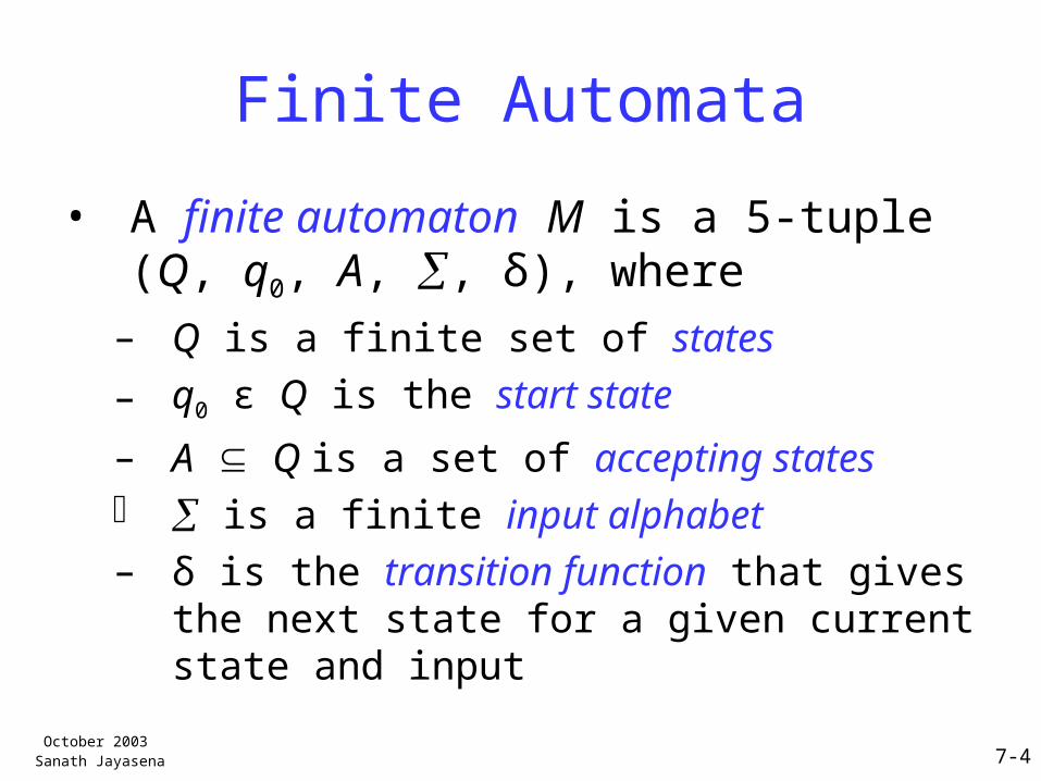
• A finite automaton M is a 5-tuple (Q, q0, A, , δ), where

– Q is a finite set of states

– q0 ε Q is the start state

– A Q is a set of accepting states is a finite input alphabet– δ is the transition function that gives the next

state for a given current state and input


7-5

How a Finite Automaton Works

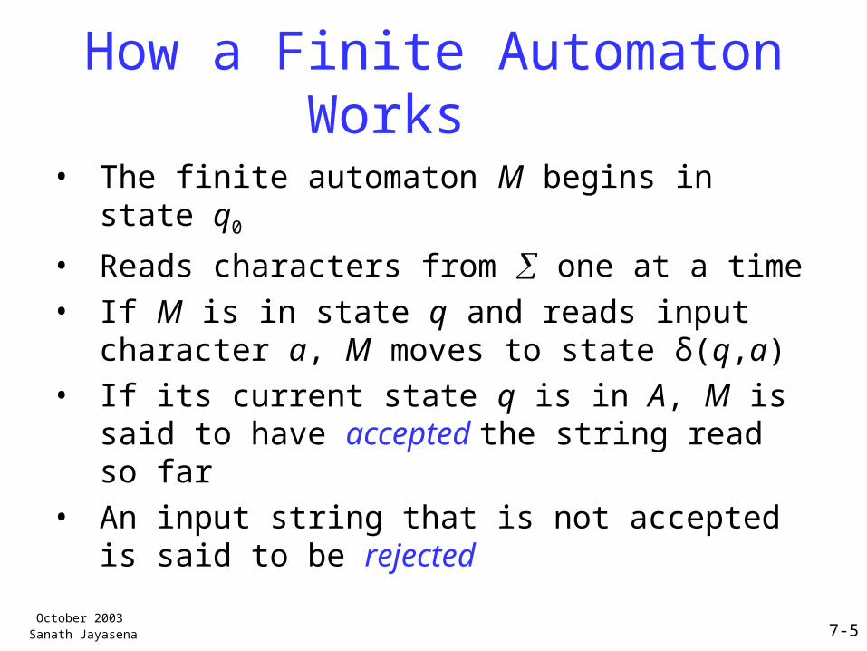
• The finite automaton M begins in state q0

• Reads characters from one at a time

• If M is in state q and reads input character a, M moves to state δ(q,a)

• If its current state q is in A, M is said to have accepted the string read so far

• An input string that is not accepted is said to be rejected


7-6

Example

1 0

0 0

input

state0

1

a b

transition table

0 1

a

a

b

b

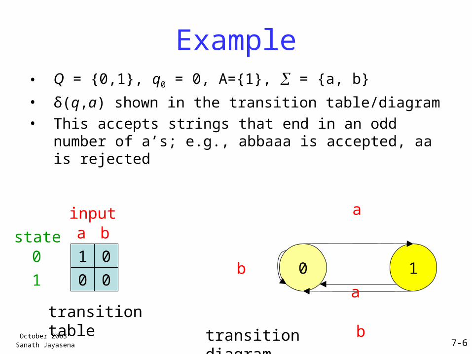
• Q = {0,1}, q0 = 0, A={1}, = {a, b}

• δ(q,a) shown in the transition table/diagram• This accepts strings that end in an odd number

of a’s; e.g., abbaaa is accepted, aa is rejected

transition diagram


7-7

String-Matching Automata

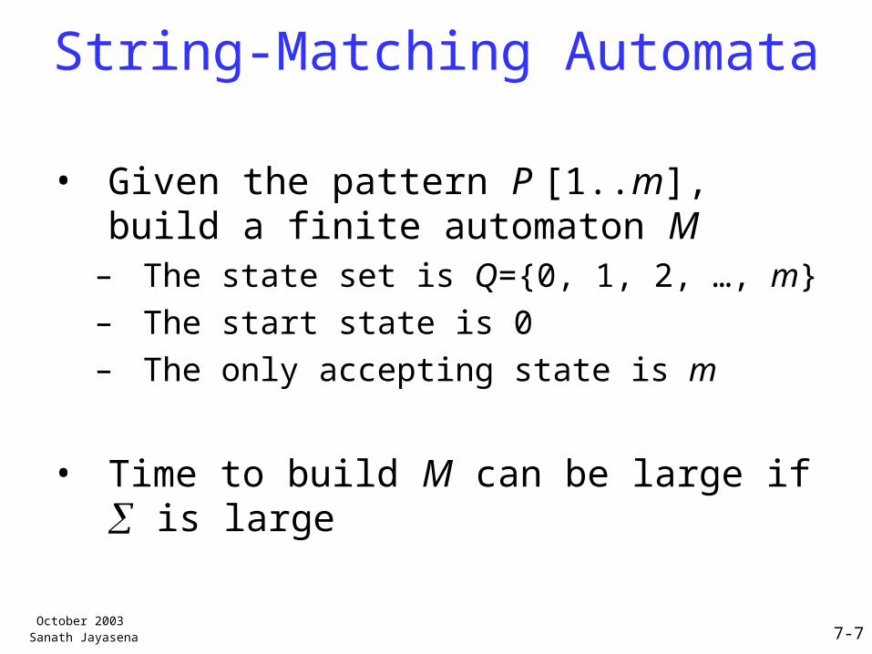
• Given the pattern P [1..m], build a finite automaton M

– The state set is Q={0, 1, 2, …, m}– The start state is 0– The only accepting state is m

• Time to build M can be large if is large


7-8

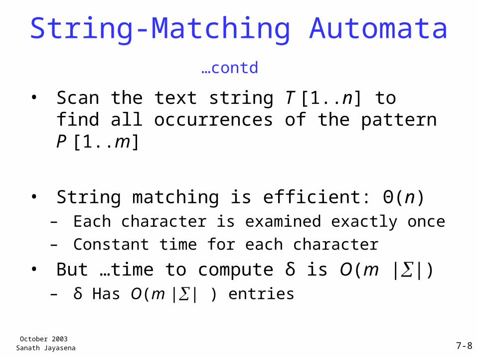
String-Matching Automata …contd

• Scan the text string T [1..n] to find all occurrences of the pattern P [1..m]

• String matching is efficient: Θ(n)– Each character is examined exactly once– Constant time for each character

• But …time to compute δ is O(m ||)– δ Has O(m || ) entries


7-9

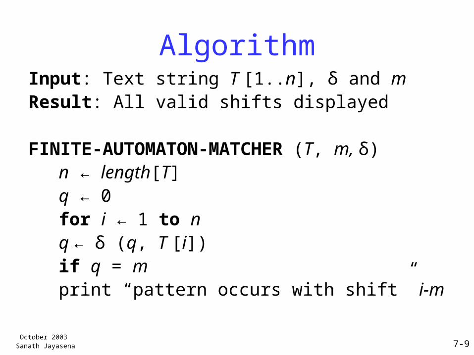
AlgorithmInput: Text string T [1..n], δ and mResult: All valid shifts displayed

FINITE-AUTOMATON-MATCHER (T, m, δ)n ← length[T]q ← 0for i ← 1 to n

q ← δ (q, T [i])if q = m

print “pattern occurs with shift” i-m


7-10

Knuth-Morris-Pratt (KMP) Method

• Avoids computing δ (transition function)

• Instead computes a prefix function π in O(m) time

– π has only m entries

• Prefix function stores info about how the pattern matches against shifts of itself

– Can avoid testing useless shifts


7-11

Terminology/Notations

• String w is a prefix of string x, if x=wy for some string y (e.g., “srilan” of “srilanka”)

• String w is a suffix of string x, if x=yw for some string y (e.g., “anka” of “srilanka”)

• The k-character prefix of the pattern P [1..m] denoted by Pk

– E.g., P0= ε, Pm = P =P [1..m]


7-12

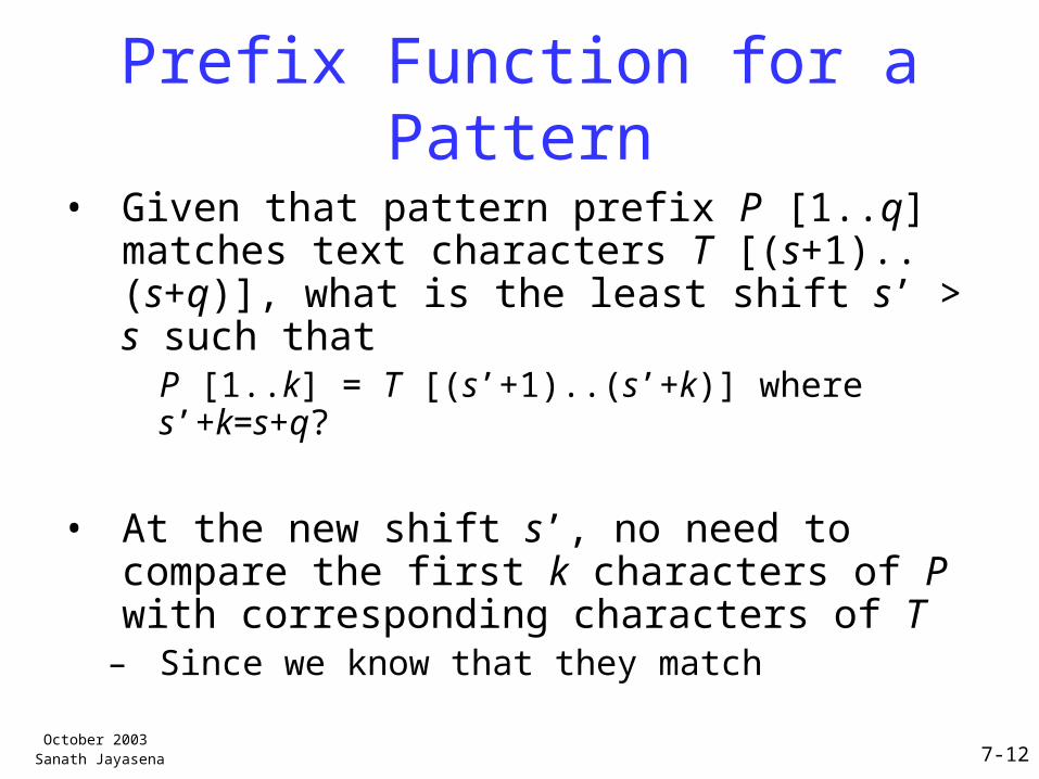
Prefix Function for a Pattern

• Given that pattern prefix P [1..q] matches text characters T [(s+1)..(s+q)], what is the least shift s’ > s such that

P [1..k] = T [(s’+1)..(s’+k)] where s’+k=s+q?

• At the new shift s’, no need to compare the first k characters of P with corresponding characters of T

– Since we know that they match


7-13

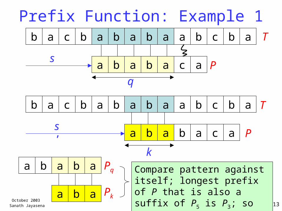
Prefix Function: Example 1b a c b a b a b a a b c b a

a b a b a c a

b a c b a b a b a a b c b a

a b a b a c a

T

Ps

s’

T

P

q

ka b a b a

a b a

Pq

Pk

Compare pattern against itself; longest prefix of P that is also a suffix of P5 is P3; so π[5]= 3


7-14

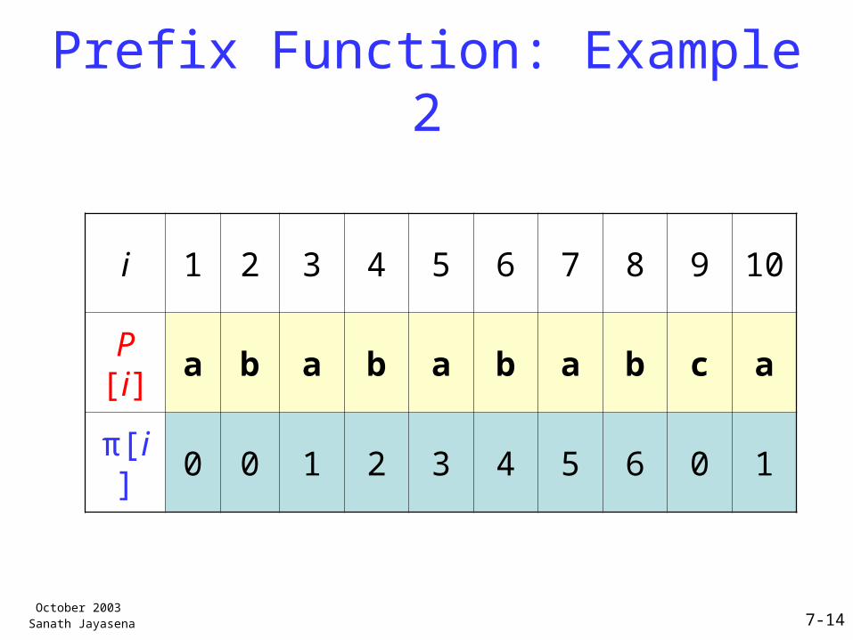
Prefix Function: Example 2

i 1 2 3 4 5 6 7 8 9 10

P [i] a b a b a b a b c a

π[i] 0 0 1 2 3 4 5 6 0 1


7-15

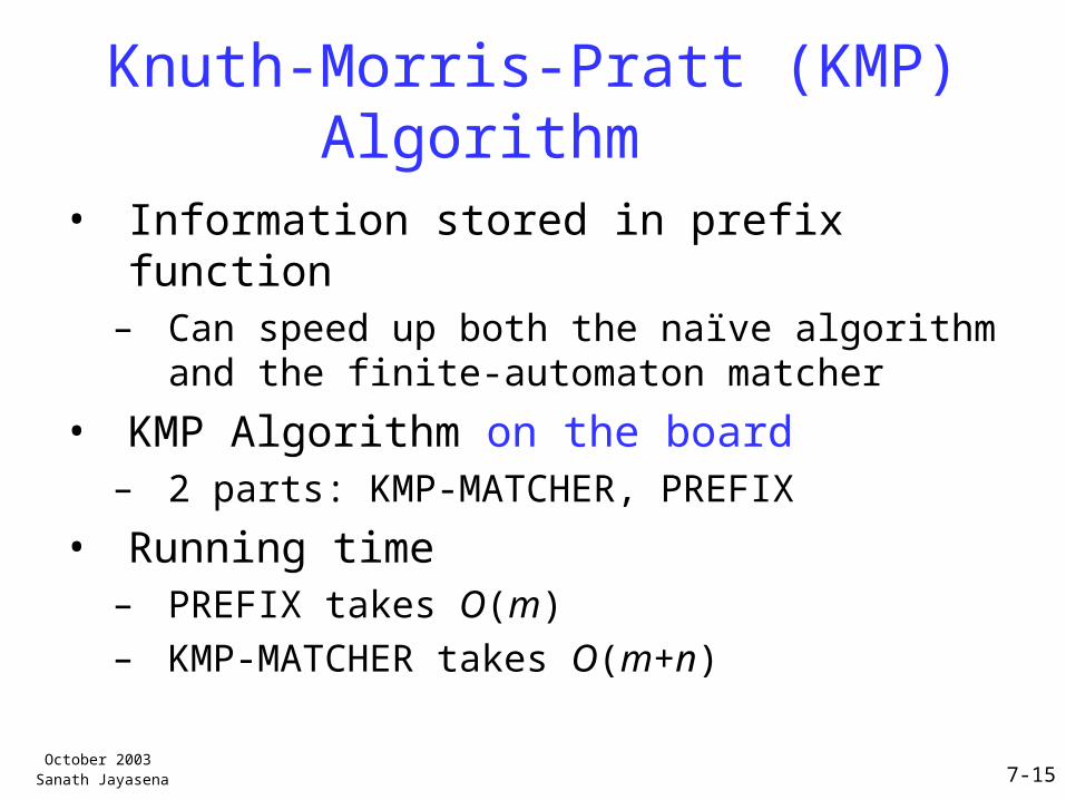
Knuth-Morris-Pratt (KMP) Algorithm

• Information stored in prefix function – Can speed up both the naïve algorithm and

the finite-automaton matcher

• KMP Algorithm on the board– 2 parts: KMP-MATCHER, PREFIX

• Running time– PREFIX takes O(m)– KMP-MATCHER takes O(m+n)

Greedy Approach to Algorithm Design


7-17

Introduction

• Greedy methods typically apply to optimization problems in which a set of choices must be made to arrive at an optimal solution

• Optimization problem– There can be many solutions – Each solution has a value– We wish to find a solution with the optimal

(minimum or maximum) value


7-18

Example Optimization Problems

• How to give a balance in minimum number of coins?

• How to allocate resources to maximize profit from your business?

• A thief has a knapsack of capacity c; what items to put in it to maximize profit?

– 0-1 knapsack problem (binary choice)– Fractional knapsack problem


7-19

Greedy Approach

• Make each choice in a locally optimal manner

– Always makes the choice that looks best at the moment

– We hope that this will lead to a globally optimal solution

• Greedy method doesn’t always give optimal solutions, but for many problems it does


7-20

Example

• A cashier gives change using coins of Rs.10, 5, 2 and 1

• Suppose the amount is Rs. 37

• Need to minimize the number of coins– Try to use the largest coin to cover the

remaining balance– So, we get 10 + 10 + 10 + 5 + 2– Does this give the optimal solution?


7-21

Elements of Greedy Approach

1. Greedy-choice property– A globally optimal solution can be arrived at

by making a locally optimal (greedy) choice– Proving this may not be trivial

2. Optimal substructure– Optimal solution to the problem contains

within it optimal solutions to subproblems


7-22

Applications of Greedy Approach

• Graph algorithms– Minimum spanning tree– Shortest path

• Data compression– Huffman coding

• Activity selection (scheduling) problems

• Fractional knapsack problem– Not the 0-1 knapsack problem


7-23

Announcements

• Assignment 4 – assigned today– due next week

• Next 2 lectures– Topic: Graphs– By Ms Sudanthi Wijewickrema

Documents

CS222 Algorithms First Semester 2003/2004