Embed Size (px)
Citation preview
Informed Search AlgorithmsCITS3001 Algorithms, Agents and Artificial Intelligence
2019, Semester 2Tim French
Department of Computer Science and Software Engineering
The University of Western Australia
Introduction
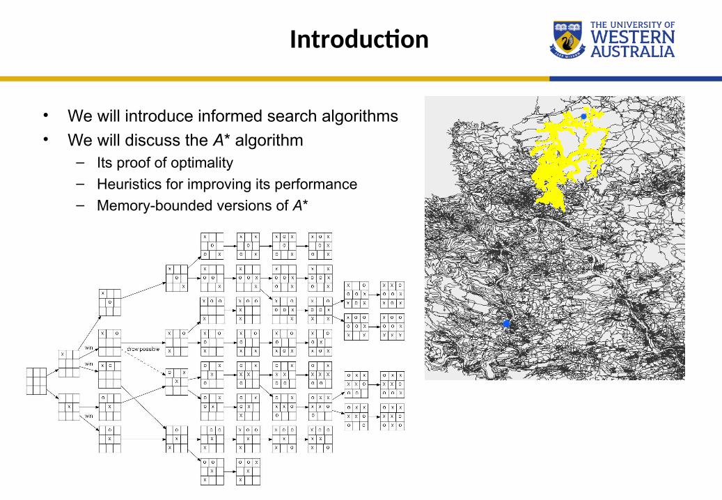
• We will introduce informed search algorithms • We will discuss the A* algorithm
– Its proof of optimality – Heuristics for improving its performance – Memory-bounded versions of A*
2
Uniformed vs Informed Search
• Recall uninformed search – Selects nodes for expansion on the basis of distance/cost from the start state
• e.g. which level in the tree is the node? – Uses only information contained in the graph
(i.e. in the problem definition) – No indication of distance to go
• Informed search – Selects nodes for expansion on the basis of some estimate of distance to the goal state – Requires additional information:
• heuristic rules, or • evaluation function
– Selects “best” node, i.e. most promising
• Examples
– Greedy search – A*
3
Greedy search of Romania
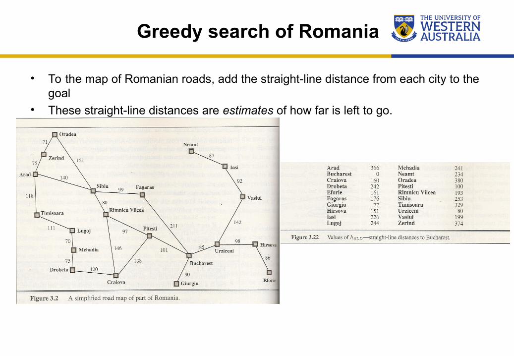
• To the map of Romanian roads, add the straight-line distance from each city to the goal
• These straight-line distances are estimates of how far is left to go.
4
Greedy Search
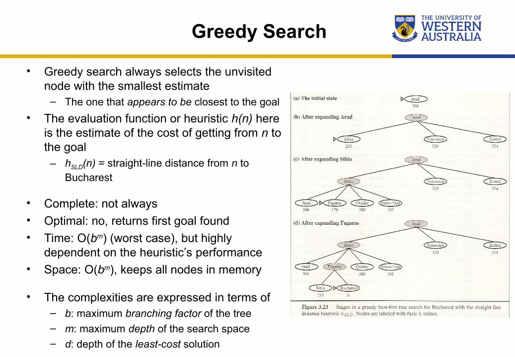
• Greedy search always selects the unvisited node with the smallest estimate
– The one that appears to be closest to the goal
• The evaluation function or heuristic h(n) here is the estimate of the cost of getting from n to the goal
– hSLD(n) = straight-line distance from n to Bucharest
• Complete: not always • Optimal: no, returns first goal found • Time: O(bm) (worst case), but highly
dependent on the heuristic’s performance • Space: O(bm), keeps all nodes in memory
• The complexities are expressed in terms of – b: maximum branching factor of the tree – m: maximum depth of the search space – d: depth of the least-cost solution 5
A* search
• Greedy search minimises estimated path-cost to goal – But it’s neither optimal nor even always complete
• Uniform-cost search minimises path-cost from the start
– Complete and optimal, but expensive
• Can we get the best of both worlds?
• Yes – use estimate of total path-cost as our heuristic
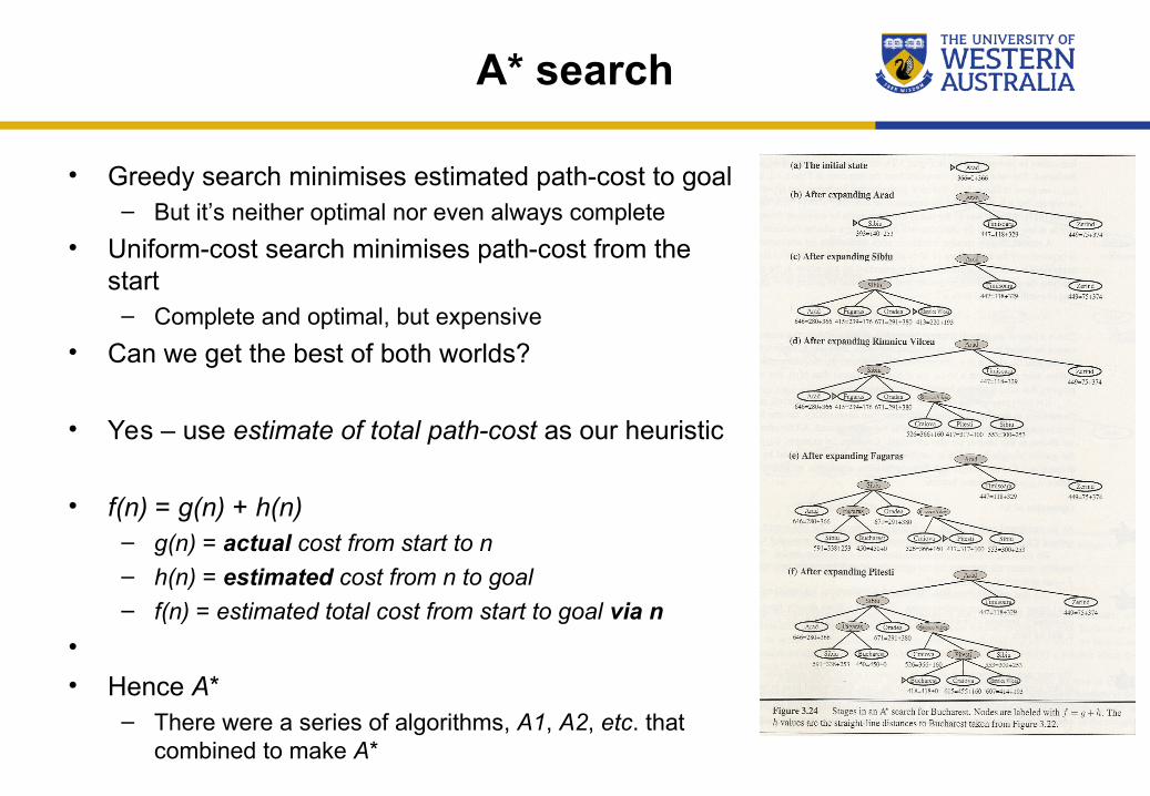
• f(n) = g(n) + h(n)
– g(n) = actual cost from start to n – h(n) = estimated cost from n to goal – f(n) = estimated total cost from start to goal via n
•
• Hence A* – There were a series of algorithms, A1, A2, etc. that
combined to make A* 6
A* demonstrations
7
A* Optimality
• A* search is complete and optimal under two conditions – The heuristic must be admissible – The costs along a given path must be monotonic
• A heuristic h is admissible iff h(n) ≤ h*(n), for all n
– h*(n) is the actual path-cost from n to the goal
• i.e. h must never over-estimate the cost – e.g. hSLD never over-estimates
• A heuristic h is monotonic iff h(n) ≤ c(n, a, n’) + h(n’), for
all n, a, n’ – n’ is a successor to n by action a – This is basically the triangle inequality – n to the goal “directly” should be no more than n to the goal
via any successor n’
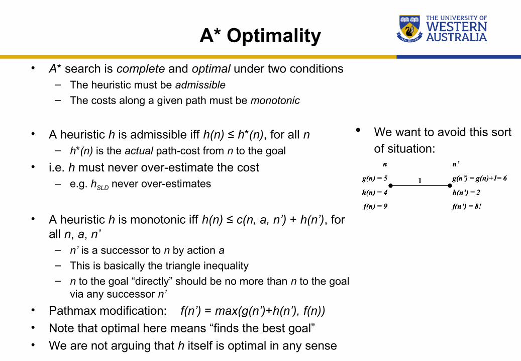
• Pathmax modification: f(n’) = max(g(n’)+h(n’), f(n)) • Note that optimal here means “finds the best goal” • We are not arguing that h itself is optimal in any sense 8
We want to avoid this sort of situation:
A* proof of optimality
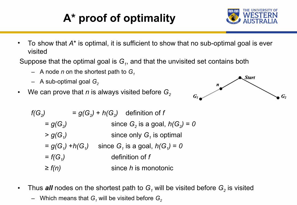
• To show that A* is optimal, it is sufficient to show that no sub-optimal goal is ever visited
Suppose that the optimal goal is G1, and that the unvisited set contains both
– A node n on the shortest path to G1
– A sub-optimal goal G2
• We can prove that n is always visited before G2
f(G2) = g(G2) + h(G2) definition of f
= g(G2) since G2 is a goal, h(G2) = 0
> g(G1) since only G1 is optimal
= g(G1) +h(G1) since G1 is a goal, h(G1) = 0
= f(G1) definition of f
≥ f(n) since h is monotonic
• Thus all nodes on the shortest path to G1 will be visited before G2 is visited
– Which means that G1 will be visited before G2
9
A* viewed operationally
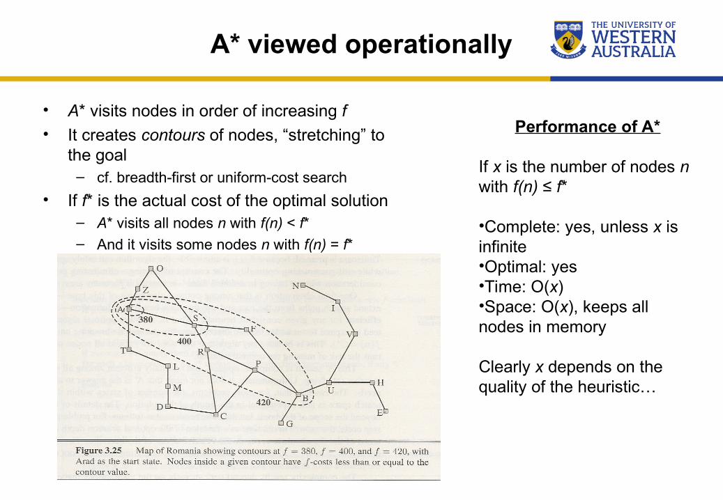
• A* visits nodes in order of increasing f• It creates contours of nodes, “stretching” to
the goal– cf. breadth-first or uniform-cost search
• If f* is the actual cost of the optimal solution– A* visits all nodes n with f(n) < f*– And it visits some nodes n with f(n) = f*
10
Performance of A*
If x is the number of nodes n with f(n) ≤ f* •Complete: yes, unless x is infinite •Optimal: yes •Time: O(x) •Space: O(x), keeps all nodes in memory Clearly x depends on the quality of the heuristic…
Assessing Heuristics
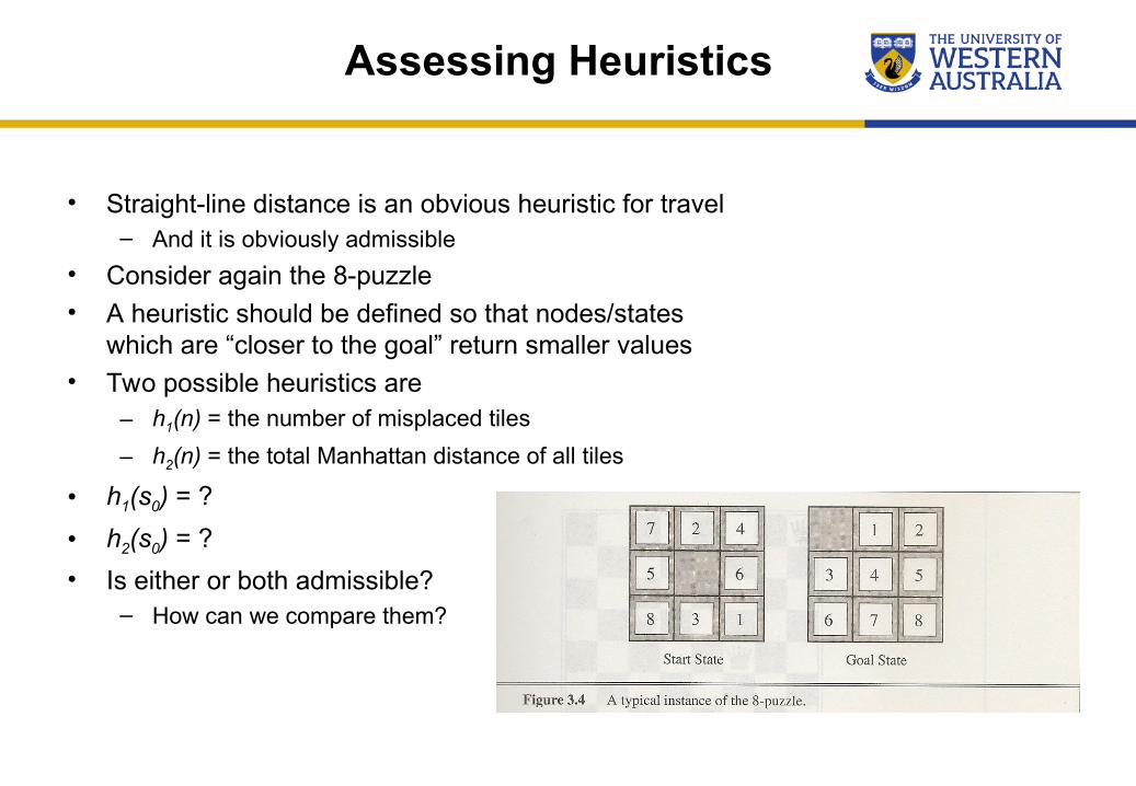
• Straight-line distance is an obvious heuristic for travel – And it is obviously admissible
• Consider again the 8-puzzle
• A heuristic should be defined so that nodes/states which are “closer to the goal” return smaller values
• Two possible heuristics are – h1(n) = the number of misplaced tiles
– h2(n) = the total Manhattan distance of all tiles
• h1(s0) = ?
• h2(s0) = ?
• Is either or both admissible? – How can we compare them?
11
Heuristic Quality
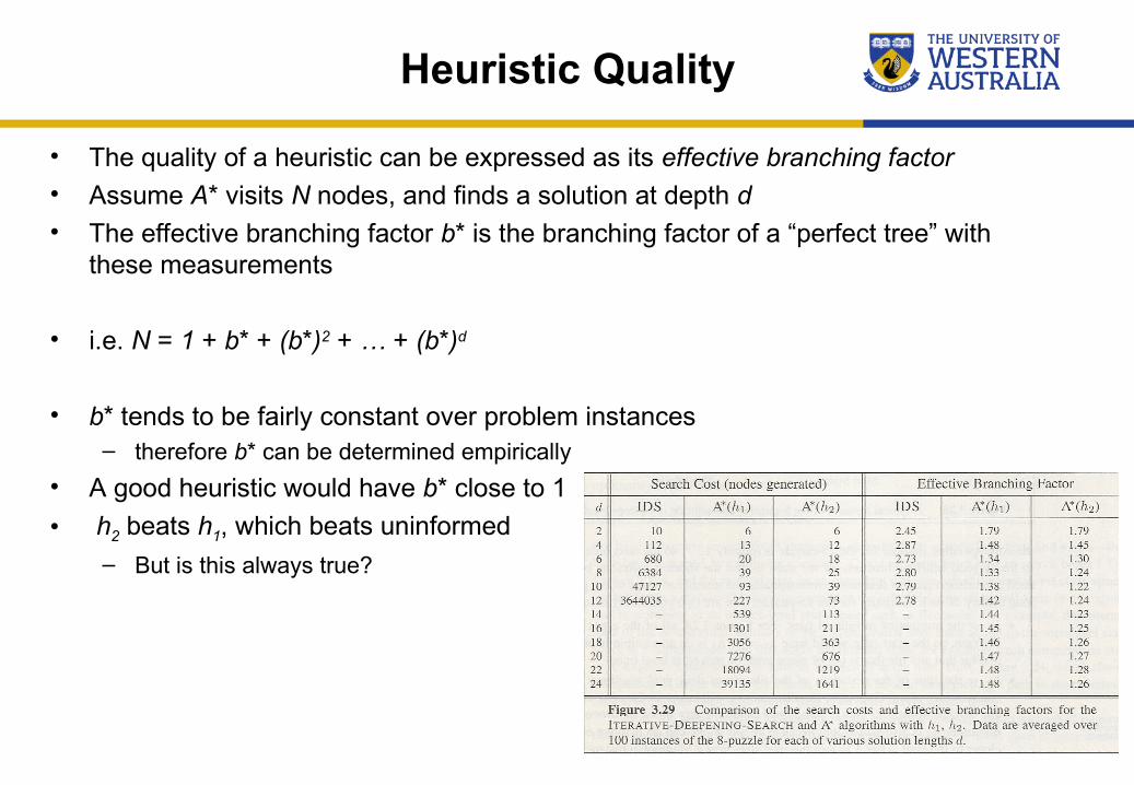
• The quality of a heuristic can be expressed as its effective branching factor • Assume A* visits N nodes, and finds a solution at depth d • The effective branching factor b* is the branching factor of a “perfect tree” with
these measurements
• i.e. N = 1 + b* + (b*)2 + … + (b*)d
• b* tends to be fairly constant over problem instances
– therefore b* can be determined empirically
• A good heuristic would have b* close to 1
• h2 beats h1, which beats uninformed
– But is this always true?
12
Heuristic dominance
• We say that h2 dominates h1 iff they are both admissible, and h2(n) ≥ h1(n), for all nodes n
– i.e. h*(n) ≥ h2(n) ≥ h1(n)
• If h2 dominates h1, then A* with h2 will usually visit fewer nodes than A* with h1
• The “proof” is obvious – A* visits all nodes n with f(n) < f* – i.e. it visits all nodes with h(n) < f* – g(n)– f* and g(n) are fixed – So if h(n) is bigger, n is less likely to be below-the-line
• Normally you should always favour a dominant heuristic– The only exception would be if it is computationally much more expensive…
• But suppose we have two admissible heuristics, neither of which dominates the other
– We can just use both!
– h(n) = max(h1(n), h2(n))
– Generalises to any number of heuristics 13
Deriving heuristics
• Coming up with good heuristics can be difficult – So can we get the computer to do it?
• Given a problem p, a relaxed version p’ of p is derived by reducing restrictions on operators
– Then the cost of an exact solution to p’ is often a good heuristic to use for p
• e.g. if the rules of the 8-puzzle are relaxed so that a tile can be moved anywhere in one go
– h1 gives the cost of the best solution
• e.g. if the rules are relaxed so that a tile can be moved to any adjacent space (whether blank or not)
– h2 gives the cost of the best solution
• We must always consider the cost of the heuristic– In the extreme case, a perfect heuristic is to perform a complete search on the original
problem
• Note that in the examples above, no searching is required – The problem has been separated into eight independent sub-problems
14
Deriving heuristics cont.
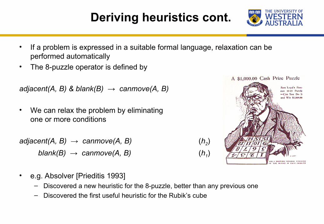
• If a problem is expressed in a suitable formal language, relaxation can be performed automatically
• The 8-puzzle operator is defined by
adjacent(A, B) & blank(B) → canmove(A, B)
• We can relax the problem by eliminating
one or more conditions
adjacent(A, B) → canmove(A, B) (h2)
blank(B) → canmove(A, B) (h1)
• e.g. Absolver [Prieditis 1993]
– Discovered a new heuristic for the 8-puzzle, better than any previous one – Discovered the first useful heuristic for the Rubik’s cube
15
Memory bounded A*
• The limiting factor on what problems A* can solve is normally space availability – cf. breadth-first search
• We solved the space problem for uninformed strategies by iterative deepening – Basically trades space for time, in the form of repeated calculation of some nodes
• We can do the same here – IDA* uses the same idea as ID – But instead of imposing a depth cut-off, it imposes an f-cost cut-off
• IDA* performs depth-limited search on all nodes n such that f(n) ≤ k
– Then if it fails, it increases k and tries again
• IDA* suffers from three problems – By how much do we increase k? – It doesn’t use all of the space available – The only information communicated between iterations is the f-cost limit
16
Simplified Memory-Bounded A*
• SMA* implements A*, but it uses all memory available
• SMA* expands the most promising node (as in A*) until memory is full
– Then it must drop a node in order to generate more nodes and continue the search
• SMA* drops the least promising node in order to make space for exploring new nodes
– But we don’t want to lose the benefit of all the work that has already been done… – It is possible that the dropped node may become important again later in the search
• When a node x is dropped, the f-cost of x is backed-up in x’s parent node – The parent thus has a lower bound on the cost of solutions in the dropped sub-tree – Note this again depends on admissibility
• If at some later point in the search, all other nodes have higher estimates than the dropped sub-tree, it is re-generated
– Again, we are trading space for time
17
SMA* example
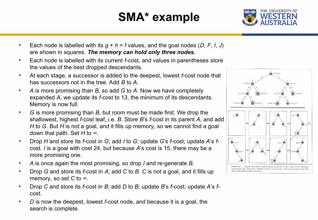
• Each node is labelled with its g + h = f values, and the goal nodes (D, F, I, J) are shown in squares. The memory can hold only three nodes.
• Each node is labelled with its current f-cost, and values in parentheses store the values of the best dropped descendants.
• At each stage, a successor is added to the deepest, lowest f-cost node that has successors not in the tree. Add B to A.
• A is more promising than B, so add G to A. Now we have completely expanded A, we update its f-cost to 13, the minimum of its descendants. Memory is now full.
• G is more promising than B, but room must be made first. We drop the shallowest, highest f-cost leaf, i.e. B. Store B’s f-cost in its parent A, and add H to G. But H is not a goal, and it fills up memory, so we cannot find a goal down that path. Set H to ∞.
• Drop H and store its f-cost in G; add I to G; update G’s f-cost; update A’s f-cost. I is a goal with cost 24, but because A’s cost is 15, there may be a more promising one.
• A is once again the most promising, so drop I and re-generate B. • Drop G and store its f-cost in A; add C to B. C is not a goal, and it fills up
memory, so set C to ∞. • Drop C and store its f-cost in B; add D to B; update B’s f-cost; update A’s f-
cost. • D is now the deepest, lowest f-cost node, and because it is a goal, the
search is complete. 18
SMA* performance
• Complete: yes, if any solution is reachable with the memory available – i.e. if a linear path to the depth d can be stored
• Optimal: yes, if an optimal solution is reachable with the memory available, o/w returns the best possible
• Time: O(x), x being the number of nodes n with f(n) ≤ f*• Space: all of it!
• In very hard cases, SMA* can end up continually switching between candidate
solutions – i.e. it spends a lot of time re-generating
dropped nodes – cf. thrashing in paging-memory systems
• But it is still a robust search process for many problems
19