Embed Size (px)
Citation preview
ALGEBRAIC NUMBER THEORY
J.S. MILNE
Abstract. These are the notes for a course taught at the University of Michiganin F92 as Math 676. They are available at www.math.lsa.umich.edu/∼jmilne/.
Please send comments and corrections to me at [email protected] (August 14, 1996.) First version on the web.v2.10 (August 31, 1998.) Fixed many minor errors; added exercises and index.
Contents
Introduction. . . . . . . . . . . . . . . . . . . . . . . . . . . . . . . . . . . . . . . . . . . . . . . . . . . . . . . . . . . . . . . . . .1
The ring of integers 1; Factorization 2; Units 4; Applications 5; A briefhistory of numbers 6; References. 7.
1. Preliminaries from Commutative Algebra . . . . . . . . . . . . . . . . . . . . . . . . . . . . 10
Basic definitions 10; Noetherian rings 10; Local rings 12; Rings of fractions12; The Chinese remainder theorem 14; Review of tensor products 15;Extension of scalars 17; Tensor products of algebras 17; Tensor products offields 17.
2. Rings of Integers . . . . . . . . . . . . . . . . . . . . . . . . . . . . . . . . . . . . . . . . . . . . . . . . . . . . . . . . 19
Symmetric polynomials 19; Integral elements 20; Review of bases of A-modules 25; Review of norms and traces 25; Review of bilinear forms 26;Discriminants 26; Rings of integers are finitely generated 28; Finding thering of integers 30; Algorithms for finding the ring of integers 33.
3. Dedekind Domains; Factorization . . . . . . . . . . . . . . . . . . . . . . . . . . . . . . . . . . . . . 37
Discrete valuation rings 37; Dedekind domains 38; Unique factorization39; The ideal class group 43; Discrete valuations 46; Integral closures ofDedekind domains 47; Modules over Dedekind domains (sketch). 48; Fac-torization in extensions 49; The primes that ramify 50; Finding factoriza-tions 53; Examples of factorizations 54; Eisenstein extensions 56.
4. The Finiteness of the Class Number . . . . . . . . . . . . . . . . . . . . . . . . . . . . . . . . . . 58
Norms of ideals 58; Statement of the main theorem and its consequences59; Lattices 62; Some calculus 67; Finiteness of the class number 69; Binaryquadratic forms 71;
5. The Unit Theorem . . . . . . . . . . . . . . . . . . . . . . . . . . . . . . . . . . . . . . . . . . . . . . . . . . . . . . 73
Statement of the theorem 73; Proof that UK is finitely generated 74; Com-putation of the rank 75; S-units 77; Finding fundamental units in real
c©1996, 1998, J.S. Milne. You may make one copy of these notes for your own personal use.i
0 J.S. MILNE
quadratic fields 77; Units in cubic fields with negative discriminant 78;Finding µ(K) 80; Finding a system of fundamental units 80; Regulators80;
6. Cyclotomic Extensions; Fermat’s Last Theorem.. . . . . . . . . . . . . . . . . . . . .82
The basic results 82; Class numbers of cyclotomic fields 87; Units in cyclo-tomic fields 87; Fermat’s last theorem 88;
7. Valuations; Local Fields . . . . . . . . . . . . . . . . . . . . . . . . . . . . . . . . . . . . . . . . . . . . . . . . 91
Valuations 91; Nonarchimedean valuations 91; Equivalent valuations 93;Properties of discrete valuations 95; Complete list of valuations for Q 95;The primes of a number field 97; Notations 97; Completions 98; Com-pletions in the nonarchimedean case 99; Newton’s lemma 102; Extensionsof nonarchimedean valuations 105; Newton’s polygon 107; Locally compactfields 108; Unramified extensions of a local field 109; Totally ramified exten-sions of K 111; Ramification groups 112; Krasner’s lemma and applications113; A Brief Introduction to PARI 115.
8. Global Fields . . . . . . . . . . . . . . . . . . . . . . . . . . . . . . . . . . . . . . . . . . . . . . . . . . . . . . . . . . . 116
Extending valuations 116; The product formula 118; Decomposition groups119; The Frobenius element 121; Examples 122; Application: the quadraticreciprocity law 123; Computing Galois groups (the hard way) 123; Comput-ing Galois groups (the easy way) 124; Cubic polynomials 126; Chebotarevdensity theorem 126; Applications of the Chebotarev density theorem 128;Topics not covered 130; More algorithms 130; The Hasse principle for qua-dratic forms 130; Algebraic function fields 130.
Exercises. . . . . . . . . . . . . . . . . . . . . . . . . . . . . . . . . . . . . . . . . . . . . . . . . . . . . . . . . . . . . . . . . .132.
It is standard to use Gothic (fraktur) letters for ideals:
a b c m n p q A B C M N P Qa b c m n p q A B C M N P Q
I use the following notations:
X ≈ Y X and Y are isomorphic;
X ∼= YX and Y are canonically isomorphicor there is a given or unique isomorphism;
Xdf= Y X is defined to be Y , or equals Y by definition;
X ⊂ Y X is a subset of Y (not necessarily proper).
Introduction 1
Introduction
An algebraic number field is a finite extension of Q; an algebraic number is anelement of an algebraic number field. Algebraic number theory studies the arithmeticof algebraic number fields — the ring of integers in the number field, the ideals inthe ring of integers, the units, the extent to which the ring of integers fails to behave unique factorization, and so on. One important tool for this is “localization”, inwhich we complete the number field relative to a metric attached to a prime ideal ofthe number field. The completed field is called a local field — its arithmetic is muchsimpler than that of the number field, and sometimes we can answer questions byfirst solving them locally, that is, in the local fields.
An abelian extension of a field is a Galois extension of the field with abelian Galoisgroup. Global class field theory classifies the abelian extensions of a number field Kin terms of the arithmetic of K; local class field theory does the same for local fields.
This course is concerned with algebraic number theory. Its sequel is on class fieldtheory (see my notes CFT).
I now give a quick sketch of what the course will cover. The fundamental theorem ofarithmetic says that integers can be uniquely factored into products of prime powers:an m = 0 in Z can be written in the form,
m = upr11 · · · prnn , u = ±1, pi prime number, ri > 0,
and this factorization is essentially unique.
Consider more generally an integral domain A. An element a ∈ A is said to be aunit if it has an inverse in A; I write A× for the multiplicative group of units in A.An element p of A is said to prime if it is neither zero nor a unit, and if
p|ab⇒ p|a or p|b.If A is a principal ideal domain, then every nonzero nonunit element a of A can bewritten in the form,
a = pr11 · · · prnn , pi prime element, ri > 0,
and the factorization is unique up to order and replacing each pi with an associate,i.e., with its product with a unit.
Our first task will be to discover to what extent unique factorization holds, or failsto hold, in number fields. Three problems present themselves. First, factorization ina field only makes sense with respect to a subring, and so we must define the “ringof integers” OK in our number field K. Secondly, since unique factorization will ingeneral fail, we shall need to find a way of measuring by how much it fails. Finally,since factorization is only considered up to units, in order to fully understand thearithmetic of K, we need to understand the structure of the group of units UK in OK.Resolving these three problems will occupy the first five sections of the course.
The ring of integers. Let K be an algebraic number field. Because K is of finitedegree over Q, every element α of K is a root of a monic polynomial
f(X) = Xn + a1Xn−1 + · · ·+ a0, ai ∈ Q.
2 Introduction
If α is a root of a monic polynomial with integer coefficients, then α is called analgebraic integer of K. We shall see that the algebraic integers form a subring OK ofK.
The criterion as stated is difficult to apply. We shall see that to prove that α isan algebraic integer, it suffices to check that its minimum polynomial (relative to Q)has integer coefficients.
Consider for example the field K = Q[√
d], where d is a square-free integer. The
minimum polynomial of α = a+ b√d, b = 0, a, b ∈ Q, is
(X − (a + b√d))(X − (a− b
√d)) = X2 − 2aX + (a2 − b2d).
Thus α is an algebraic integer if and only if
2a ∈ Z, a2 − b2d ∈ Z.
From this it follows easily that
OK = Z[√d] = m+ n
√d | m,n ∈ Z if d ≡ 2, 3 mod 4,
and
OK = m+ n1 +√d
2| m,n ∈ Z if d ≡ 1 mod 4,
i.e., OK is the set of sums m′ + n′√d with m′ and n′ either both integers or both
half-integers.
Let ζd be a primitive dth root of 1, for example, ζd = exp(2πi/d), and letK = Q[ζd].Then we shall see that
OK = Z[ζd] = ∑
miζid | mi ∈ Z.
as one would hope.
Factorization. An element p of an integral domain A is said to be irreducible if itis neither zero nor a unit, and can’t be written as a product of two nonunits. Forexample, a prime element is (obviously) irreducible. A ring A is a unique factorizationdomain if every nonzero nonunit element of A can be expressed as a product ofirreducible elements in essentially one way. Is OK a unique factorization domain?No, not in general!
In fact, we shall see that each element of OK can be written as a product ofirreducible elements (this is true for all Noetherian rings) — it is the uniqueness thatfails.
For example, in Z[√−5] we have
6 = 2 · 3 = (1 +√−5)(1−√−5).
To see that 2, 3, 1+√−5, 1−√−5 are irreducible, and no two are associates, we use
the norm map
Nm : Q[√−5]→ Q, a+ b
√−5 → a2 + 5b2.
For α ∈ OK, we have
Nm(α) = 1 ⇐⇒ αα = 1 ⇐⇒ α is a unit. (*)
Introduction 3
If 1+√−5 = αβ, then Nm(αβ) = Nm(1+
√−5) = 6. Thus Nm(α) = 1, 2, 3, or 6. Inthe first case, α is a unit, the second and third cases don’t occur, and in the fourthcase β is a unit. A similar argument shows that 2, 3, and 1 − √−5 are irreducible.Next note that (*) implies that associates have the same norm, and so it remains toshow that 1 +
√−5 and 1−√−5 are not associates, but
1 +√−5 = (a + b
√−5)(1−√−5)has no solution with a, b ∈ Z.
Why does unique factorization fail inOK? The problem is that irreducible elementsin OK need not be prime. In the above example, 1 +
√−5 divides 2 · 3 but it dividesneither 2 nor 3. In fact, in an integral domain in which factorizations exist (e.g. aNoetherian ring), factorization is unique if all irreducible elements are prime.
What can we recover? Consider
210 = 6 · 35 = 10 · 21.If we were naive, we might say this shows factorization is not unique in Z; instead, werecognize that there is a unique factorization underlying these two decompositions,namely,
210 = (2 · 3)(5 · 7) = (2 · 5)(3 · 7).The idea of Kummer and Dedekind was to enlarge the set of “prime numbers” sothat, for example, in Z[
√−5] there is a unique factorization,
6 = (p1 · p2)(p3 · p4) = (p1 · p3)(p2 · p4),underlying the above factorization; here the pi are “ideal prime factors”.
How do we define “ideal factors”? Clearly, an ideal factor should be character-ized by the algebraic integers it divides. Moreover divisibility by a should have thefollowing properties:
a|0; a|a, a|b⇒ a|a± b; a|a⇒ a|ab for all b ∈ OK.If in addition division by a has the property that
a|ab⇒ a|a or a|b,then we call a a “prime ideal factor”. Since all we know about an ideal factor is theset of elements it divides, we may as well identify it with this set. Thus an idealfactor is a set of elements a ⊂ OK such that
0 ∈ a; a, b ∈ a⇒ a± b ∈ a; a ∈ a⇒ ab ∈ a for all b ∈ OK ;it is prime if an addition,
ab ∈ a⇒ a ∈ a or b ∈ a.
Many of you will recognize that an ideal factor is what we now call an ideal, and aprime ideal factor is a prime ideal.
There is an obvious notion of the product of two ideals:
ab|c ⇐⇒ c =∑
aibi, a|ai, b|bi.In other words,
ab = ∑
aibi | ai ∈ a, bi ∈ b.
4 Introduction
One see easily that this is again an ideal, and that if
a = (a1, ..., am) and b = (b1, ..., bn)
then
a · b = (a1b1, a1b2, ..., aibj, ..., ambn).
With these definitions, one recovers unique factorization: if a = 0, then there is anessentially unique factorization:
(a) = pr11 · · · prnn with each pi a prime ideal.
In the above example,
(6) = (2, 1 +√−5)(2, 1−√−5)(3, 1 +√−5)(3, 1−√−5).
In fact, I claim
(2, 1 +√−5)(2, 1−√−5) = (2)
(3, 1 +√−5)(3, 1−√−5) = (3)
(2, 1 +√−5)(3, 1 +√−5) = (1 +
√−5)(2, 1−√−5)(3, 1−√−5) = (1−√−5).
For example, (2, 1 +√−5)(2, 1 − √−5) = (4, 2 + 2
√−5, 2− 2√−5, 6). Since every
generator is divisible by 2, (2, 1 +√−5)(2, 1−√−5) ⊂ (2). Conversely,
2 = 6− 4 ∈ (4, 2 + 2√−5, 2− 2
√−5, 6)and so (2, 1 +
√−5)(2, 1 − √−5) = (2). Moreover, the four ideals (2, 1 +√−5),
(2, 1−√−5), (3, 1 +√−5), and (3, 1−√−5) are all prime. For example
Z[√−5]/(3, 1−√−5) = Z/(3),
which is an integral domain.
How far is this from what we want, namely, unique factorization of elements? Inother words, how many “ideal” elements have we had to add to our “real” elementsto get unique factorization. In a certain sense, only a finite number: we shall seethat there is a finite set of ideals a1, ..., ah such that every ideal is of the form ai · (a)for some i and some a ∈ OK . Better, we shall construct a group I of “fractional”ideals in which the principal fractional ideals (a), a ∈ K×, form a subgroup P of finiteindex. The index is called the class number hK of K. We shall see that
hK = 1 ⇐⇒ OK is a principal ideal domain ⇐⇒ OK is a unique factorization domain.
Units. Unlike Z, OK can have an infinite number of units. For example, (1 +√2) is
a unit of infinite order in Z[√2] :
(1 +√2)(−1 +√2) = 1; (1 +
√2)m = 1 for m ≥ 1.
In fact Z[√2]× = ±(1 +√2)m | m ∈ Z, and so
Z[√2]× ≈ ±1 × free abelian group of rank 1.
Introduction 5
In general, we shall show (unit theorem) that the roots of 1 in K form a finite groupµ(K), and that
O×K ≈ µ(K)× Zr (as an abelian group);
moreover, we shall find r.
Applications. I hope to give some applications. One motivation for the developmentof algebraic number theory was the attempt to prove Fermat’s last “theorem”, i.e.,that there are no integer solutions to the equation
Xm + Y m = Zm
when m ≥ 3, except for the obvious solutions.
When m = 3, this can proved by the method of “infinite descent”, i.e., fromone solution, you show that you can construct a smaller solution, which leads to acontradiction1. The proof makes use of the factorization
Y 3 = Z3 −X3 = (Z −X)(Z2 +XZ +X2),
and it was recognized that a stumbling block to proving the theorem for larger m isthat no such factorization exists into polynomials with integer coefficients. This ledpeople to look at more general factorizations.
In a very famous incident, the French mathematician Lame gave a talk at theParis Academy in 1847 in which he claimed to prove Fermat’s last theorem using thefollowing ideas. Let p > 2 be a prime, and suppose x, y, z are nonzero integers suchthat
xp + yp = zp.
Write
xp = zp − yp =∏
(z − ζ iy), 0 ≤ i ≤ p− 1, ζ = e2πi/p.
He then showed how to obtain a smaller solution to the equation, and hence a contra-diction. Liouville immediately questioned a step in Lame’s proof in which he assumedthat, in order to show that each factor (z − ζ iy) is a pth power, it suffices to showthat the factors are relatively prime in pairs and their product is a pth power. Infact, Lame couldn’t justify his step (Z[ζ] is not always a principal ideal domain), andFermat’s last theorem remains unproven to the present day2. However, shortly afterLame’s embarrassing lecture, Kummer used his results on the arithmetic of the fieldsQ[ζ] to prove Fermat’s last theorem for all “regular primes”.
Another application is to finding Galois groups. The splitting field of a polynomialf(X) ∈ Q[X] is a Galois extension of Q. In the basic graduate algebra course (seeFT), we learn how to compute the Galois group only when the degree is very small(e.g., ≤ 3). By using algebraic number theory one can write down an algorithm todo it for any degree.
1The simplest proof by infinite descent is that showing that√2 is irrational.
2Written in 1992.
6 Introduction
A brief history of numbers. Prehistory (??-1600). Basic arithmetic was devel-oped in many parts of the world thousands of years ago. For example, 3,500 yearsago the Babylonians apparently knew how to construct the solutions to
X2 + Y 2 = Z2.
At least they knew that
(4961)2 + (6480)2 = (8161)2
which could scarcely be found by trial and error. The Chinese remainder theorem wasknown in China, thousands of years ago. The Greeks knew the fundamental theoremof arithmetic, and, of course, Euclid’s algorithm.
Fermat (1601–1665). Apart from his famous last “theorem”, he invented themethod of infinite descent. He also posed the problem of finding integer solutions tothe equation,
X2 − AY 2 = 1, A ∈ Z, (*)
which is essentially the problem3 of finding the units in Z[√A]. The English math-
ematicians found an algorithm for solving the problem, but neglected to show thatthe algorithm always works.
Euler (1707–1783). Among many other works, he discovered the quadratic reci-procity law.
Lagrange (1736–1813). He proved that the algorithm for solving (*) always leadsto a solution.
Legendre (1752–1833). He proved the “Hasse principle” for quadratic forms inthree variables over Q: the quadratic form Q(X, Y, Z) has a nontrivial zero in Q ifand only if it has one in R and the congruence Q ≡ 0 mod pn has a nontrivial solutionfor all p and n.
Gauss (1777–1855). He found many proofs of the quadratic reciprocity law:(p
q
)(q
p
)= (−1)(p−1)(q−1)/4, p, q odd primes.
He studied the Gaussian integers Z[i] in order to find a quartic reciprocity law. Hestudied the classification of binary quadratic forms over Z which, as we shall see, isclosely related to the problem of finding the class numbers of quadratic fields.
Dirichlet (1805–1859). He proved the following “unit theorem”: let α be a rootof a monic irreducible polynomial f(X) with integer coefficients; suppose that f(X)has r real roots and 2s complex roots; then Z[α]× is a finitely generated group ofrank r + s− 1. He proved a famous analytic formula for the class number.
Kummer (1810–1893). He made a deep study of the arithmetic of cyclotomic fields,motivated by a search for higher reciprocity laws. His general result on Fermat’s lasttheorem is the most important to date.
Hermite (1822–1901).
Eisenstein (1823–1852).
3The Indian mathematician Bhaskara (12th century) knew general rules for finding solutions tothe equation.
Introduction 7
Kronecker (1823–1891). He developed an alternative to Dedekind’s ideals. Healso had one of the most beautiful ideas in mathematics, the Kronecker liebster Ju-gendtraum, for generating abelian extensions of number fields.
Riemann (1826–1866). Made the Riemann hypothesis.
Dedekind (1831–1916). He was the first mathematician to formally define fields— many of the basic theorems on fields in basic graduate algebra courses were provedby him. He also found the correct general definition of the ring of integers in anumber field, and he proved that ideals factor uniquely into products of prime ideals.Moreover, he improved the Dirichlet unit theorem.
Weber (1842–1913). Made important progress in class field theory and the Kro-necker Jugendtraum.
Hensel (1861–1941). He introduced the notion of the p-adic completion of a field.
Hilbert (1862–1943). He wrote a very influential book on algebraic number theoryin 1897, which gave the first systematic account of the theory. Some of his famousproblems were on number theory, and have also been influential.
Takagi (1875–1960). He made very important advances in class field theory.
Hecke (1887–1947). Introduced Hecke L-series.
Artin (1898–1962). He found the “Artin reciprocity law”, which is the maintheorem of class field theory.
Hasse (1898–1979). Proved the Hasse principle for all quadratic forms over numberfields.
Weil (1906–1998). Defined the Weil group, which enabled him to give a commongeneralization of Artin L-series and Hecke L-series.
Chevalley (1909–??). The main statements of class field theory are purely al-gebraic, but all the earlier proofs used analysis. Chevalley gave a purely algebraicproof.
Iwasawa (1917– ). He introduced an important new approach into the study ofalgebraic number theory which was suggested by the theory of curves over finite fields.
Tate (1925– ). With Artin, he gave a complete cohomological treatment of classfield theory. With Lubin he introduced a concrete way of generating abelian exten-sions of local fields.
Langlands (1936– ). “Langlands’s philosophy” is a vast series of conjectures that,among other things, contains a nonabelian class field theory.
References. Books on algebraic number theory.
Artin, E., Theory of Algebraic Numbers, Gottingen notes, 1959. Elegant; good exam-ples; but he adopts a valuation approach rather than the ideal-theoretic approach weuse in this course.
Artin, E., Algebraic Numbers and Algebraic Functions, Nelson, 1968. Covers both thenumber field and function field case.
Borevich, Z. I., and Shafarevich, I. R., Number Theory, Academic Press, 1966.In addition to basic algebraic number theory, it contains material on diophantineequations.
8 Introduction
Cassels, J.W.S., and Frohlich, A., Eds., Algebraic Number Theory, Academic Press,1967. The proceedings of an instructional conference. Many of the articles are excel-lent, for example, those of Serre and Tate on class field theory.
Cassels, J.W.S., Local fields, London Math. Soc., 1986. Concentrates on local fields,but does also deal with number fields, and it gives some interesting applications.
Cohn, P.M., Algebraic Numbers and Algebraic Functions, Chapman and Hall, 1991.The valuation approach.
Dedekind, R., Theory of Algebraic Integers, Cambridge Univ. Press, 1996 (translationof the 1877 French original). Develops the basic theory through the finiteness of theclass number in a way that is surprising close to modern approach in, for example,these notes.
Edwards, H., Fermat’s Last Theorem: A Genetic Introduction to Algebraic NumberTheory, Springer, 1977. A history of algebraic number theory, concentrating on theefforts to prove Fermat’s last theorem. Edwards is one of the most reliable writers onthe history of number theory.
Frohlich, A., and Taylor, M.J., Algebraic Number Theory, Cambridge Univ. Press,1991. Lots of good problems.
Goldstein, L.J., Analytic Number Theory, Prentice-Hall, 1971. Similar approach toLang 1970, but the writing is a bit careless. Sometimes includes more details thanLang, and so it is probably easier to read.
Janusz, G. Algebraic Number Fields, Second Edn, Amer. Math. Soc., 1996. It coversboth algebraic number theory and class field theory, which it treats from a lowbrowanalytic/algebraic approach. In the past, I sometimes used the first edition as a textfor this course and its sequel.
Lang, S. Algebraic Numbers Theory, Addison-Wesley, 1970. Difficult to read unlessyou already know it, but it does contain an enormous amount of material. Covers alge-braic number theory, and it does class field theory from a highbrow analytic/algebraicapproach.
Marcus, D. Number Fields, Springer, 1977. This is a rather pleasant down-to-earthintroduction to algebraic number theory.
Narkiewicz, W. Algebraic Numbers, Springer, 1990. Encyclopedic coverage of alge-braic number theory.
Samuel, P., Algebraic Theory of Numbers, Houghton Mifflin, 1970. A very easy treat-ment, with lots of good examples, but doesn’t go very far.
Serre, J.-P. Corps Locaux, Hermann, 1962 (Translated as Local Fields). A classic. Anexcellent account of local fields, cohomology of groups, and local class field theory.The local class field theory is bit dated (Lubin-Tate groups weren’t known when thebook was written) but this is the best book for the other two topics.
Weil, A., Basic Number Theory, Springer, 1967. Very heavy going, but you will learna lot if you manage to read it (covers algebraic number theory and class field theory).
Weiss, R., Algebraic Number Theory, McGraw-Hill, 1963. Very detailed; in fact a bittoo fussy and pedantic.
9
Weyl, H., Algebraic Theory of Numbers, Princeton Univ. Press, 1940. One of the firstbooks in English; by one of the great mathematicians of the twentieth century. Id-iosyncratic — Weyl prefers Kronecker to Dedekind, e.g., see the section “Our disbeliefin ideals”.
Computational Number Theory.
Cohen, H., A Course in Computational Number Theory, Springer, 1993.
Lenstra, H., Algorithms in Algebraic Number Theory, Bull. Amer. Math. Soc., 26,1992, 211–244.
Pohst and Zassenhaus, Algorithmic Algebraic Number Theory, Cambridge Univ.Press, 1989.
The two books provide algorithms for most of the constructions we make in thiscourse. The first assumes the reader knows number theory, whereas the second de-velops the whole subject algorithmically. Cohen’s book is the more useful as a sup-plement to this course, but wasn’t available when these notes were first written, andso the references are to Pohst and Zassenhaus. While the books are concerned withmore-or-less practical algorithms for fields of small degree and small discriminant,Lenstra’s article concentrates on finding “good” general algorithms.
Additional references
Atiyah, M.F., and MacDonald, I.G., Introduction to Commutative Algebra, Addison-Wesley, 1969. I use this as a reference on commutative algebra.
Washington, L., Introduction to Cyclotomic Fields, 1982. This is the best book oncyclotomic fields.
I will sometimes refer to my other course notes:
GT: Group Theory (594)FT: Fields and Galois Theory (594)EC: Elliptic Curves (679).CFT: Class Field Theory (776).
10
1. Preliminaries from Commutative Algebra
Many results that were first proved for rings of integers in number fields are truefor more general commutative rings, and it is more natural to prove them in thatcontext.
Basic definitions. All rings will be commutative, and have an identity element (i.e.,an element 1 such that 1a = a for all a ∈ A), and a homomorphism of rings will mapthe identity element to the identity element.
A ring B together with a homomorphism of rings A→ B will be referred to as anA-algebra. We use this terminology mainly when A is a subring of B. In this case, forelements β1, ..., βm of B, A[β1, ..., βm] denotes the smallest subring of B containing Aand the βi. It consists of all polynomials in the βi with coefficients in A, i.e., elementsof the form ∑
ai1...imβi11 ...β
imm , ai1...im ∈ A.
We also refer to A[β1, ..., βm] as the A-subalgebra of B generated by the βi, and whenB = A[β1, ..., βm] we say that the βi generate B as an A-algebra.
For elements a1, a2, . . . of A, (a1, a2, . . . ) denotes the smallest ideal containing theai. It consists of finite sums
∑ciai, ci ∈ A, and it is called the ideal generated by
a1, a2, . . . . When a and b are ideals in A, we define
a + b = a + b | a ∈ a, b ∈ b.It is again an ideal in A — in fact, it is the smallest ideal containing both a and b. Ifa = (a1, ..., am) and b = (b1, ..., bn), then a + b = (a1, ..., am, b1, ..., bn).
Given an ideal a in A, we can form the quotient ring A/a. Let f : A → A/a bethe homomorphism a → a+ a; then b → f−1(b) defines a one-to-one correspondencebetween the ideals of A/a and the ideals of A containing a, and
A/f−1(b)≈→ (A/a)/b.
A proper ideal a of A is prime if ab ∈ a ⇒ a or b ∈ a. An ideal a is prime if andonly if the quotient ring A/a is an integral domain. An element p of A is said to beprime if (p) is a prime ideal; equivalently, if p|ab⇒ p|a or p|b.
A proper ideal a in A is maximal if there does not exist an ideal b, a b A. Anideal a is maximal if and only if A/a is a field. Every proper ideal a of A is containedin a maximal ideal — if A is Noetherian (see below) this is obvious; otherwise theproof requires Zorn’s lemma. In particular, every nonunit in A is contained in amaximal ideal.
There are the implications: A is a Euclidean domain ⇒ A is a principal idealdomain⇒ A is a unique factorization domain (see any good graduate algebra course).
Noetherian rings.
Lemma 1.1. The following conditions on a ring A are equivalent:
(a) Every ideal in A is finitely generated.
1. Preliminaries from Commutative Algebra 11
(b) Every ascending chain of ideals
a1 ⊂ a2 ⊂ · · · ⊂ an ⊂ · · ·becomes stationary, i.e., after a certain point an = an+1 = · · · .
(c) every nonempty set S of ideals in A has a maximal element a, i.e., there is anideal a in S that is not contained in any other ideal in S.
Proof. (a)⇒(b): Let a = ∪ai; it is an ideal, and hence is finitely generated, saya = (a1, . . . , ar). For some n, an will contain all the ai, and so an = an+1 = · · · = a.
(b)⇒(a): Consider an ideal a. If a = (0), then a is generated by the empty set, whichis finite. Otherwise there is an element a1 ∈ a, a1 = 0. If a = (a1), then a is certainlyfinitely generated. If not, there is an element a2 ∈ a such that (a1) (a1, a2).Continuing in this way, we obtain a chain of ideals
(a1) (a1, a2) · · · .This process must eventually stop with (a1, . . . , an) = a.
(b)⇒(c): Let a1 ∈ S. If a1 is not a maximal element of S, then there is an a2 ∈ Ssuch that a1 a2. If a2 is not maximal, then there is an a3 etc.. From (b) we knowthat this process will lead to a maximal element after only finitely many steps.
(c)⇒(b): Apply (c) to the set S = a1, a2, . . . .
A ring A satisfying the equivalent conditions of the lemma is said to be Noetherian4
A famous theorem of Hilbert states that k[X1, ..., Xn] is Noetherian. In practice,almost all the rings that arise naturally in algebraic number theory or algebraic geom-etry are Noetherian, but not all rings are Noetherian. For example, k[X1, . . . , Xn, . . . ]is not Noetherian: X1, . . . , Xn is a minimal set of generators for the ideal (X1, . . . , Xn)in k[X1, . . . , Xn], and X1, . . . , Xn, . . . is a minimal set of generators for the ideal(X1, . . . , Xn, . . . ) in k[X1, . . . , Xn, . . . ]
Proposition 1.2. Every nonzero nonunit element of a Noetherian integral do-main can be written as a product of irreducible elements.
Proof. We shall need to use that
(a) ⊂ (b) ⇐⇒ b|a, with equality ⇐⇒ b = a× unit.
The first assertion is obvious. For the second, note that if a = bc and b = ad thena = bc = adc, and so dc = 1. Hence both c and d are units.
Suppose the statement is false, and choose an element a ∈ A which contradictsthe statement and is such that (a) is maximal among the ideals generated by suchelements (here we use that A is Noetherian). Since a can not be written as a productof irreducible elements, it is not itself irreducible, and so a = bc with b and c nonunits.Clearly (b) ⊃ (a), and the ideals can’t be equal for otherwise c would be a unit. Fromthe maximality of (a), we deduce that b can be written as a product of irreducibleelements, and similarly for c. Thus a is a product of irreducible elements, and wehave a contradiction.
4After Emmy Noether (1882–1935).
12 1. Preliminaries from Commutative Algebra
Local rings. A ring A is said to local if it has exactly one maximal ideal m. In thiscase, A× = A m (complement of m in A).
Lemma 1.3 (Nakayama’s lemma). Let A be a local Noetherian ring, and let a bea proper ideal in A. Let M be a finitely generated A-module, and define
aM = ∑ aimi | ai ∈ a, mi ∈M.(a) If aM = M , then M = 0.(b) If N is a submodule of M such that N + aM = M , then N = M.
Proof. (a) Suppose M = 0. Among the finite sets of generators for M , chooseone m1, ..., mk having the fewest elements. From the hypothesis, we know that wecan write
mk = a1m1 + a2m2 + ...akmk some ai ∈ a.
Then
(1− ak)mk = a1m1 + a2m2 + ... + ak−1mk−1.
As 1−ak is not in m, it is a unit, and so m1, ..., mk−1 generates M . This contradictsour choice of m1, ..., mk, and so M = 0.
(b) We shall show that a(M/N) = M/N , and then apply the first part of the lemmato deduce that M/N = 0. Consider m + N , m ∈ M . From the assumption, we canwrite
m = n +∑
aimi, with ai ∈ a, mi ∈M.
Whence
m+N =∑
aimi +N =∑
ai(mi +N) (definition of the action of A on M/N),
and so m+N ∈ a(M/N).
The hypothesis that M be finitely generated in the lemma is crucial. For example,if A is a local integral domain with maximal ideal m = 0, then mM = M for any fieldM containing A but M = 0.
Rings of fractions. Let A be an integral domain; there is a field K ⊃ A, called thefield of fractions of A, with the property that every c ∈ K can be written in the formc = ab−1, a, b ∈ A, b = 0. For example, Q is the field of fractions of Z, and k(X) isthe field of fractions of k[X].
Let A be an integral domain with field of fractions K. A subset S of A is saidto be multiplicative if 0 /∈ S, 1 ∈ S, and S is closed under multiplication. If S is amultiplicative subset, then we define
S−1A = a/b ∈ K | b ∈ S.It is obviously a subring of K.
Example 1.4. (a) Let t be a nonzero element of A; then
Stdf= 1,t,t2,...
1. Preliminaries from Commutative Algebra 13
is a multiplicative subset of A, and we (sometimes) write At for S−1t A. For example,
if d is a nonzero integer,
Zd = a/dn ∈ Q | a ∈ Z, n ≥ 0.It consists of those elements of Q whose denominator divides some power of d.
(b) If p is a prime ideal, then Sp = A p is a multiplicative set (if neither a nor bbelongs to p, then ab does not belong to p). We write Ap for S
−1p A. For example,
Z(p) = m/n ∈ Q | n is not divisible by p.Proposition 1.5. Let A be an integral domain, and let S be a multiplicative subset
of A. The map
p → S−1pdf= a/s | a ∈ p, s ∈ S
is a bijection from the set of prime ideals in A such that p∩S = ∅ to the set of primeideals in S−1A; the inverse map is q → q ∩ A.
Proof. It is easy to see that
p a prime ideal disjoint from S ⇒ S−1p is a prime ideal,
q a prime ideal in S−1A⇒ q ∩A is a prime ideal disjoint from S,
and so we only have to show that the two maps are inverse, i.e.,
(S−1p) ∩A = p and S−1(q ∩A) = q.
(S−1p)∩A = p : Clearly (S−1p)∩A ⊃ p. For the reverse inclusion, let a/s ∈ (S−1p)∩A,a ∈ p, s ∈ S. Consider the equation a
s· s = a ∈ p. Both a/s and s are in A, and so
at least one of a/s or s is in p (because it is prime); but s /∈ p (by assumption), andso a/s ∈ p.
S−1(q ∩ A) = q : Clearly S−1(q ∩ A) ⊂ q because q ∩ A ⊂ q and q is an ideal inS−1A. For the reverse inclusion, let b ∈ q. We can write it b = a/s with a ∈ A, s ∈ S.Then a = s · (a/s) ∈ q ∩A, and so a/s = (s · (a/s))/s ∈ S−1(q ∩A).
Example 1.6. (a) If p is a prime ideal in A, then Ap is a local ring (because pcontains every prime ideal disjoint from Sp).
(b) We list the prime ideals in some rings:
Z: (2), (3), (5), (7), (11), . . . , (0);
Z2: (3), (5), (7), (11), . . . , (0);
Z(2): (2), (0);
Z42: (5), (11), (13), . . . , (0);
Z/(42): (2), (3), (7).
Note that in general, for t a nonzero element of an integral domain,
prime ideals of At ↔ prime ideals of A not containing t
prime ideals of A/(t) ↔ prime ideals of A containing t.
14 1. Preliminaries from Commutative Algebra
The Chinese remainder theorem. Recall the classical form of the theorem: letd1, ..., dn be integers, relatively prime in pairs; then for any integers x1, ..., xn, theequations
x ≡ xi (mod di)
have a simultaneous solution x ∈ Z; if x is one solution, then the other solutions arethe integers of the form x+md, m ∈ Z, where d =
∏di.
We want to translate this in terms of ideals. Integers m and n are relatively primeif and only if (m,n) = Z, i.e., if and only if (m) + (n) = Z. This suggests definingideals a and b in a ring A to be relatively prime if a + b = A.
If m1, ..., mk are integers, then ∩(mi) = (m) where m is the least common multipleof the mi. Thus ∩(mi) ⊃ (
∏mi) =
∏(mi). If the mi are relatively prime in pairs,
then m =∏
mi, and so we have ∩(mi) =∏(mi). Note that in general,
a1 · a2 · · · an ⊂ a1 ∩ a2 ∩ ... ∩ an.
These remarks suggest the following statement.
Theorem 1.7. Let a1, ..., an be ideals in a ring A, relatively prime in pairs. Thenfor any elements x1, ..., xn of A, the equations
x ≡ xi (mod ai)
have a simultaneous solution x ∈ A; if x is one solution, then the other solutions arethe elements of the form x + a with a ∈ ∩ai; moreover, ∩ai =
∏ai. In other words,
the natural maps give an exact sequence
0→ a→ A→n∏i=1
A/ai → 0
with a = ∩ai =∏
ai.
Proof. Suppose first that n = 2. As a1 + a2 = A, there are elements ai ∈ ai suchthat a1 + a2 = 1. The element x =df a1x2 + a2x1 has the required property.
For each i we can find elements ai ∈ a1 and bi ∈ ai such that
ai + bi = 1, all i ≥ 2.
The product∏
i≥2(ai + bi) = 1, and lies in a1 +∏
i≥2 ai, and so
a1 +∏i≥2
ai = A.
We can now apply the theorem in the case n = 2 to obtain an element y1 of A suchthat
y1 ≡ 1 mod a1, y1 ≡ 0 mod∏i≥2
ai.
These conditions imply
y1 ≡ 1 mod a1, y1 ≡ 0 mod aj, all j > 1.
Similarly, there exist elements y2, ..., yn such that
yi ≡ 1 mod ai, yi ≡ 0 mod aj for j = i.
The element x =∑
xiyi now satisfies the requirements.
1. Preliminaries from Commutative Algebra 15
It remains to prove that ∩ai =∏
ai. We have already noted that ∩ai ⊃∏
ai. Firstsuppose that n = 2, and let a1 + a2 = 1, as before. For c ∈ a1 ∩ a2, we have
c = a1c+ a2c ∈ a1 · a2which proves that a1∩a2 = a1a2. We complete the proof by induction. This allows usto assume that
∏i≥2 ai = ∩i≥2ai. We showed above that a1 and
∏i≥2 ai are relatively
prime, and so
a1 · (∏i≥2
ai) = a1 ∩ (∏i≥2
ai) = ∩ai.
The theorem extends to A-modules.
Theorem 1.8. Let a1, ..., an be ideals in A, relatively prime in pairs, and let M bean A-module. There is an exact sequence:
0→ aM → M →∏i
M/aiM → 0
with a =∏
ai = ∩ai.This has an elementary proof (see Janusz 1996, p. 9), but I prefer to use tensor
products, which I now review.
Review of tensor products. Let M , N , and P be A-modules. A mapping f : M ×N → P is said to be A-bilinear if
f(m+m′, n) = f(m,n) + f(m′, n); f(m,n+ n′) = f(m,n) + f(m,n′)
f(am, n) = af(m,n) = f(m, an), a ∈ A, m,m′ ∈M, n, n′ ∈ N,
i.e., if it is linear in each variable. A pair (Q, f) consisting of an A-module Q andan A-bilinear map f : M × N → Q is called the tensor product of M and N ifany other A-bilinear map f ′ : M × N → P factors uniquely into f ′ = α f withα : Q → P A-linear. The tensor product exists, and is unique (up to a uniqueisomorphism). We denote it by M ⊗A N , and we write (m,n) → m ⊗ n for f .The pair (M ⊗A N, (m,n) → m ⊗ n) is characterized by each of the following twoconditions:
(a) The map M × N → M ⊗A N is A-bilinear, and any other A-bilinear mapM×N → P is of the form (m,n) → α(m⊗n) for a unique A-linear map α : M⊗AN →P ; thus
BilinA(M ×N,P ) = HomA(M ⊗A N,P ).
(b) As an A-module, M ⊗A N generated by the symbols m ⊗ n, m ∈ M , n ∈ N ,which satisfy the relations
(m+m′)⊗ n = m⊗ n+m′ ⊗ n; m⊗ (n+ n′) = m⊗ n +m⊗ n′
am⊗ n = a(m⊗ n) = m⊗ an.
Tensor products commute with direct sums: there is a canonical isomorphism
(⊕iMi)⊗A (⊕jNj)≈→⊕i,jMi ⊗A Nj, (
∑mi)⊗ (
∑nj) →
∑mi ⊗ nj .
16 1. Preliminaries from Commutative Algebra
It follows that if M and N are free A-modules5 with bases (ei) and (fj) respectively,then M ⊗A N is a free A-module with basis (ei ⊗ fj). In particular, if V and W arevector spaces over a field k of dimensions m and n respectively, then V ⊗k W is avector space over k of dimension mn.
Let α : M → N and β : M ′ → N ′ be A-linear maps. Then
(m,n) → α(m)⊗ β(n) : M ×N →M ′ ⊗A N ′
is A-bilinear, and therefore factors through M × N → M ⊗A N . Thus there is anA-linear map α⊗ β : M ⊗A N → M ′ ⊗A N ′ such that
(α⊗ β)(m⊗ n) = α(m)⊗ β(n).
Remark 1.9. Let α : km → km and β : kn → kn be two matrices, regarded as alinear maps. Then α ⊗ β is a linear map kmn → kmn. Its matrix with respect tothe canonical basis is called the Kronecker product of the two matrices. (Kroneckerproducts of matrices pre-date tensor products by about 70 years.)
Lemma 1.10. If α : M → N and β : M ′ → N ′ are surjective, then so also is
α⊗ β : M ⊗A N →M ′ ⊗A N ′.
Proof. Recall that M ′⊗N ′ is generated as an A-module by the elementsm′⊗n′,m′ ∈ M ′, n′ ∈ N ′. By assumption m′ = α(m) for some m ∈ M and n′ = β(n) forsome n ∈ N , and so m′ ⊗ n′ = α(m)⊗ β(n) = (α⊗ β)(m⊗ n). Therefore Im(α⊗ β)contains a set of generators for M ′ ⊗A N ′ and so it is equal to it.
One can also show that if
M ′ → M → M ′′ → 0
is exact, then so also is
M ′ ⊗A P → M ⊗A P → M ′′ ⊗A P → 0.
For example, if we tensor the exact sequence
0→ a→ A→ A/a→ 0
with M , we obtain an exact sequence
a⊗A M →M → (A/a)⊗A M → 0
The image of a⊗M in M is
aMdf= ∑aimi | ai ∈ a, mi ∈M,
and so we obtain from the exact sequence that
M/aM ∼= (A/aA)⊗A M (1.11).
By way of contrast, if M → N is injective, then M ⊗A P → N ⊗A P need notbe injective. For example, take A = Z, and note that (Z m→ Z) ⊗Z (Z/mZ) equals
Z/mZ m→ Z/mZ, which is the zero map.
5Let M be an A-module. Elements e1, . . . , em form a basis for M if every element of M canbe expressed uniquely as a linear combination of the ei’s with coefficients in A. Then Am → M ,(a1, . . . , am) →
∑aiei, is an isomorphism of A-modules, and M is said to be a free A-module of
rank m.
1. Preliminaries from Commutative Algebra 17
Proof of Theorem 1.8. Return to the situation of the theorem. When we ten-sor the isomorphism
A/a∼=→ ∏
A/ai
with M , we get an isomorphism
M/aM ∼= (A/a)⊗A M∼=→ ∏
(A/ai)⊗A M ∼= ∏M/aiM,
as required.
Extension of scalars. If A→ B is an A-algebra and M is an A-module, then B⊗AMhas a natural structure of a B-module for which
b(b′ ⊗m) = bb′ ⊗m, b, b′ ∈ B, m ∈M.
We say that B ⊗AM is the B-module obtained from M by extension of scalars. Themap m → 1 ⊗m : M → B ⊗A M is uniquely determined by the following universalproperty: it isA-linear, and for any A-linear map α : M → N fromM into aB-moduleN , there is a unique B-linear map α′ : B ⊗A M → N such that α′(1⊗ m) = α(m).Thus α → α′ defines an isomorphism
HomA(M,N)→ HomB(B ⊗A M,N), N a B-module).
For example, A ⊗A M = M . If M is a free A-module with basis e1, . . . , em, thenB ⊗A M is a free B-module with basis 1⊗ e1, . . . , 1⊗ em.
Tensor products of algebras. If f : A→ B and g : A→ C are A-algebras, then B⊗AChas a natural structure of an A-algebra: the product structure is determined by therule
(b⊗ c)(b′ ⊗ c′) = bb′ ⊗ cc′
and the map A→ B ⊗A C is a → f(a)⊗ 1 = 1⊗ g(a).
For example, there is a canonical isomorphism
a⊗ f → af : K ⊗k k[X1, . . . , Xm]→ K[X1, . . . , Xm] (1.12).
Tensor products of fields. We are now able to computeK⊗kΩ ifK is a finite separablefield extension of k and Ω is an arbitrary field extension of k. According to theprimitive element theorem (FT, 5.1), K = k[α] for some α ∈ K. Let f(X) be theminimum polynomial of α. By definition this means that the map g(X) → g(α)determines an isomorphism
k[X]/(f(X))→ K.
Hence
K ⊗k Ω ∼= (k[X]/(f(X)))⊗ Ω ∼= Ω[X]/(f(X))
by (1.11) and (1.12). Because K is separable over k, f(X) has distinct roots. There-fore f(X) factors in Ω[X] into monic irreducible polynomials
f(X) = f1(X) · · · fr(X)
18 1. Preliminaries from Commutative Algebra
that are relatively prime in pairs. We can apply the Chinese Remainder Theorem todeduce that
Ω[X]/(f(X)) =
r∏i=1
Ω[X]/(fi(X)).
Finally, Ω[X]/(fi(X)) is a finite separable field extension of Ω of degree deg fi. Thuswe have proved the following result:
Theorem 1.13. Let K be a finite separable field extension of k, and let Ω be anarbitrary field extension. Then K⊗kΩ is a product of finite separable field extensionsof Ω,
K ⊗k Ω =r∏i=1
Ωi.
If α is a primitive element for K/k, then the image αi of α in Ωi is a primitiveelement for Ωi/Ω, and if f(X) and fi(X) are the minimum polynomials for α and αirespectively, then
f(X) =
r∏i=1
fi(X).
Example 1.14. Let K = Q[α] with α algebraic over Q. Then
C⊗Q K ∼= C⊗Q (Q[X]/(f(X))) ∼= C[X]/((f(X)) ∼= ∏C[X]/(X − αi) ≈ Cr.
Here α1, . . . , αr are the conjugates of α in C. The composite of β → 1 ⊗ β : K →C⊗Q K with projection onto the ith factor is
∑ajα
j →∑ajα
ji .
Finally we note that it is essential to assume in (1.13) that K is separable over k.If not, there will be an α ∈ K such that αp = a ∈ k but α /∈ k. The ring K ⊗k Kcontains an element β = (α ⊗ 1− 1⊗ α) = 0 such that
βp = a⊗ 1− 1⊗ a = a(1⊗ 1) − a(1⊗ 1) = 0.
Hence K ⊗k K contains a nonzero nilpotent element, and so can’t be a product offields.
2. Rings of Integers 19
2. Rings of Integers
Let A be an integral domain, and let L be a field containing A. An element α of Lis said to be integral over A if it is a root of a monic polynomial with coefficients inA, i.e., if it satisfies an equation
αn + a1αn−1 + ... + an = 0, ai ∈ A.
Before proving that the elements of L integral over A form a ring, we need to reviewsymmetric polynomials.
Symmetric polynomials. A polynomial P (X1, ..., Xr) ∈ A[X1, . . . , Xr] is said tobe symmetric if it is unchanged when its variables are permuted, i.e., if
P (Xσ(1), . . . , Xσ(r)) = P (X1, . . . , Xr), all σ ∈ Symr.
For example
S1 =∑
Xi, S2 =∑i<j
XiXj, . . . , Sr = X1 · · ·Xr,
are all symmetric. These particular polynomials are called the elementary symmetricpolynomials.
Theorem 2.1. (Symmetric function theorem) Let A be a ring. Every symmetricpolynomial P (X1, ..., Xr) in A[X1, ..., Xr] is equal to a polynomial in the symmetricelementary polynomials with coefficients in A, i.e., P ∈ A[S1, ..., Sr].
Proof. We define an ordering on the monomials in the Xi by requiring that
Xi11 Xi2
2 · · ·Xirr > Xj1
1 Xj22 · · ·Xjr
r
if either
i1 + i2 + · · ·+ ir > j1 + j2 + · · · + jr
or equality holds and, for some s,
i1 = j1, . . . , is = js, but is+1 > js+1.
Let Xk11 · · ·Xkr
r be the highest monomial occurring in P with a coefficient c = 0.Because P is symmetric, it contains all monomials obtained from Xk1
1 · · ·Xkrr by
permuting the X’s. Hence k1 ≥ k2 ≥ · · · ≥ kr.
Clearly, the highest monomial in Si is X1 · · ·Xi, and it follows easily that thehighest monomial in Sd11 · · ·Sdr
r is
Xd1+d2+···+dr1 Xd2+···+dr
2 · · ·Xdrr .
Therefore
P (X1, . . . , Xr)− cSk1−k21 Sk2−k32 · · ·Skrr < P (X1, . . . , Xr).
We can repeat this argument with the polynomial on the left, and after a finite numberof steps, we will arrive at a representation of P as a polynomial in S1, . . . , Sr.
20 2. Rings of Integers
Let f(X) = Xn + a1Xn−1 + · · · + an ∈ A[X], and let α1, . . . , αn be the roots of
f(X) in some ring containing A, so that f(X) =∏(X − αi) in some larger ring.
Then
a1 = −S1(α1, . . . , αn), a2 = S2(α1, . . . , αn), . . . , an = ±Sn(α1, . . . , αn).
Thus the elementary symmetric polynomials in the roots of f(X) lie in A, and so thetheorem implies that every symmetric polynomial in the roots of f(X) lies in A.
Integral elements.
Theorem 2.2. The set of elements of L integral over A forms a ring.
Proof. I shall give two proofs, first an old-fashioned proof, and later the slickmodern proof. Suppose α and β are integral over A; I’ll prove only that α + β isintegral overA since the same proof works for α−β and αβ. Let Ω be an algebraicallyclosed field containing L.
We are given that α is a root of a polynomial f(X) = Xm + a1Xm−1 + · · · + am,
ai ∈ A. Write
f(X) =∏
(X − αi), αi ∈ Ω.
Similarly, β is a root of polynomial g(X) = Xn + b1Xn−1 + · · · + bn, bi ∈ A, and we
write
f(X) =∏
(X − βi), βi ∈ Ω.
Let γ1, γ2, ..., γmn be the family of numbers of the form αi + βj (or αi − βj, or αiβj).I claim that h(X) =df
∏(X − γij) has coefficients in A. This will prove that α+ β is
integral over A because h is monic and h(α+ β) = 0.
The coefficients of h are symmetric in the αi and βj. Let P (α1, ..., αm, β1, ..., βn) beone of these coefficients, and regard it as a polynomial Q(β1, ..., βn) in the β’s withcoefficients in A[α1, ..., αm]; then its coefficients are symmetric in the αi, and so lie inA. Thus P (α1, ..., αm, β1, ..., βn) is a symmetric polynomial in the β’s with coefficientsin A — it therefore lies in A, as claimed.
Definition 2.3. The ring of elements of L integral over A is called the integralclosure of A in L. The integral closure of Z in an algebraic number field L is calledthe ring of integers OL in L.
Next we want to see that L is the field of fractions of OL; in fact we can provemore.
Proposition 2.4. Let K be the field of fractions of A, and let L be a field con-taining K. If α ∈ L is algebraic over K, then there exists a d ∈ A such that dα isintegral over A.
Proof. By assumption, α satisfies an equation
αm + a1αm−1 + · · ·+ am = 0, ai ∈ K.
2. Rings of Integers 21
Let d be a common denominator for the ai, so that dai ∈ A for all i, and multiplythrough the equation by dm :
dmαm + a1dmαm−1 + ... + amd
m = 0.
We can rewrite this as
(dα)m + a1d(dα)m−1 + · · ·+ amd
m = 0.
As a1d, ... , amdm ∈ A, this shows that dα is integral over A.
Corollary 2.5. Let A be an integral domain with field of fractions K, and let Lbe an algebraic extension of K. If B is the integral closure of A in L, then L is thefield of fractions of B.
Proof. The proposition shows that every α ∈ L can be written α = β/d withβ ∈ B, d ∈ A.
Definition 2.6. A ring A is integrally closed if it is its own integral closure in itsfield of fractions K, i.e., if
α ∈ K, α integral over A⇒ α ∈ A.
Proposition 2.7. A unique factorization domain (e.g. a principal ideal domain)is integrally closed.
Proof. Suppose a/b, a, b ∈ A, is an element of the field of fractions of A that isintegral over A. If b is a unit, then a/b ∈ A. Otherwise we may suppose that thereis an irreducible element p of A dividing b but not a. As a/b is integral over A, itsatisfies an equation
(a/b)n + a1(a/b)n−1 + · · ·+ an = 0, ai ∈ A.
On multiplying through by bn, we obtain the equation
an + a1an−1b+ ... + anb
n = 0.
The element p then divides every term on the left except an, and hence must dividean. Since it doesn’t divide a, this is a contradiction.
Hence it is easy to get examples where unique factorization fails — take any ringwhich is not integrally closed, for example, Z[
√5].
Example 2.8. (a) The rings Z and Z[i] are integrally closed — both are principalideal domains.
(b) Let k be a field. I claim that the integral closure of k[S1, ..., Sm] ink(X1, . . . , Xm) is k[X1, . . . , Xm] (here the Si are the elementary symmetric poly-nomials).
Let f ∈ k(X1, . . . , Xm) be integral over k[S1, . . . , Sm]. Then f is integral overk[X1, . . . , Xm], which is a unique factorization domain, and hence is integrally closedin its field of fractions. Thus f ∈ k[X1, . . . , Xm].
Conversely, let f ∈ k[X1, . . . , Xm]. Then f is a root of the monic polynomial∏σ∈Symm
(T − f(Xσ(1), . . . , Xσ(m))).
22 2. Rings of Integers
The coefficients of this polynomial are symmetric polynomials in theXi, and therefore(see 2.1) lie in k[S1, . . . , Sr].
Proposition 2.9. Let K be the field of fractions of A, and let L be an extensionof K of finite degree. Assume A is integrally closed. An element α of L is integralover A if and only if its minimum polynomial over K has coefficients in A.
Proof. Assume α is integral over A, so that
αm + a1αm−1 + ... + am = 0, some ai ∈ A.
Let α′ be a conjugate of α, i.e., a root of the minimum polynomial of α over K. Thenthere is an K-isomorphism
σ : K[α]→ K[α′], σ(α) = α′;
see6 FT. On applying σ to the above equation we obtain the equation
α′m + a1α′m−1 + ... + am = 0,
which shows that α′ is integral over A. Hence all the conjugates of α are integral overA, and it follows from (2.2) that the coefficients of f(X) are integral over A. Theylie in K, and A is integrally closed, and so they lie in A. This proves the “only if”part of the statement, and the “if” part is obvious.
Remark 2.10. As we noted in the introduction, this makes it easy to computesome rings of integers. For example, an element α ∈ Q[
√d] is integral over Z if and
only if its trace and norm both lie in Z.
Proposition 2.11. Let L be a field containing A. An element α of L is integralover A if and only if there is a nonzero finitely generated A-submodule of L such thatαM ⊂M (in fact, we can take M = A[α], the A-subalgebra generated by α).
Proof. ⇒: Suppose
αn + a1αn−1 + ... + an = 0, ai ∈ A.
Then the A-submodule M of L generated by 1, α, ..., αn−1 has the property thatαM ⊂M .
⇐=: We shall need to apply Cramer’s rule. As usually stated (in linear algebracourses) this says that, if
m∑j=1
cijxj = di, i = 1, . . . , m,
then
xj = det(Cj)/det(C)
where C = (cij) and Cj is obtained from C by replacing the elements of the jth columnwith the dis. When one restates the equation as
det(C) · xj = det(Cj)
6If f(X) is the minimum polynomial of α, hence also of α′, over K, then the map h(X) →h(α) : K[X] → K[α] induces an isomorphism τ : K[X]/(f(X)) → K[α]. Similarly, h(X) →h(α′) : K[X]→ K[α′] induces an isomorphism τ ′ : K[X]/(f(X)) → K[α′], and we set σ = τ ′ τ−1.
2. Rings of Integers 23
it becomes true over any ring (whether or not det(C) is invertible). The proof iselementary—essentially it is what you wind up with when you eliminate the othervariables (try it for m = 2). Alternatively, expand out
detCj =
∣∣∣∣∣∣c11 . . . −∑
c1jxj . . . c1m· · · · · ·
cm1 . . . −∑cmjxj . . . cmm
∣∣∣∣∣∣using standard properties of determinants.
Now let M be a nonzero A-module in L such that αM ⊂M , and let v1, . . . , vn bea finite set of generators for M . Then, for each i,
αvi =∑
aijvj, some aij ∈ A.
We can rewrite this system of equations as
(α− a11)v1 − a12v2 − a13v3 − · · · = 0
−a21v1 + (α− a22)v2 − a23v3 − · · · = 0
· · · = 0.
Let C be the matrix of coefficients on the left-hand side. Then Cramer’s rule tellsus that det(C) · vi = 0 for all i. Since at least one vi is nonzero and we are workinginside the field L, this implies that det(C) = 0. On expanding out the determinant,we obtain an equation
αn + c1αn−1 + c2α
n−2 + · · · + cn = 0, ci ∈ A.
We now give a second proof that if A is a subring of a field L and B is the set ofelements of L that are integral over A, then B is a ring. Let α and β be two elementsof L integral over A, and let M and N be finitely generated A-modules in L suchthat αM ⊂ M and βN ⊂ N . Define
MN = ∑
mini | mi ∈M, ni ∈ N.Then:
(a) MN is an A-submodule of L (easy);(b) it is finitely generated — if e1, . . . , em generates M and f1, . . . , fn generates
N , then e1f1, . . . , eifj, . . . , emfn generates MN ;(c) it is stable under multiplication by αβ and by α± β.
We can now apply (2.11) to deduce that αβ and α± β are integral over A.
Proposition 2.12. If B is integral over A and finitely generated as an A-algebra,then it is finitely generated as an A-module.
Proof. First consider the case that B is generated as an A-algebra by a singleelement, say B = A[β]. By assumption
βn + a1βn−1 + · · ·+ an = 0, some ai ∈ A.
Every element of B is a finite sum
c0 + c1β + c2β2 + · · ·+ cNβ
N ,
24 2. Rings of Integers
and we can exploit the preceding equality to replace βn (successively) with a linearcombination of lower powers of β. Thus every element of B is of the form
c0 + c1β + c2β2 + · · ·+ cn−1βn−1,
i.e., 1, β, β2, . . . , βn−1 generate B as an A-module. In order to pass to the generalcase, we need a lemma.
Lemma 2.13. Let A ⊂ B ⊂ C be rings. If B is finitely generated as an A-module,and C is finitely generated as a B-module, then C is finitely generated as an A-module.
Proof. If β1, ..., βm is a set of generators for B as an A-module, and γ1, ..., γnis a set of generators for C as a B-module, then βiγj is a set of generators for C asan A-module.
We now complete the proof of (2.12). Let β1, . . . , βm generate B as an A-algebra,and consider
A ⊂ A[β1] ⊂ A[β1, β2] ⊂ · · · ⊂ A[β1, ..., βm] = B.
We saw above that A[β1] is finitely generated as an A-module. Since A[β1, β2] =A[β1][β2], and β2 is integral over A[β1] (because it is over A), the same observationshows that A[β1, β2] is finitely generated as a A[β1]-module. Now the lemma showsthat A[β1, β2] is finitely generated as an A-module. Continuing in this fashion, wefind that B is finitely generated as an A-module.
Proposition 2.14. Consider integral domains A ⊂ B ⊂ C; if B is integral overA, and C is integral over B, then C is integral over A.
Proof. Let γ ∈ C ; it satisfies an equation
γn + b1γn−1 + · · · + bn = 0, bi ∈ B.
Let B ′ = A[b1, ..., bn]. Then B ′ is finitely generated as an A-module (by the lastproposition), and γ is integral over B ′ (by our choice of the bi), and so B ′[γ] is finitelygenerated as an A-module. Since γB ′[γ] ⊂ B ′[γ], Proposition 2.11 shows that γ isintegral over A.
Corollary 2.15. The integral closure of A in an algebraic extension L of its fieldof fractions is integrally closed.
Proof. Let B be the integral closure of A in L. We know from (2.5) that L is thefield of fractions of B. If γ ∈ L is integral over B, then the proposition shows that itis integral over A, and so lies in B.
Remark 2.16. In particular, the ring of integers in a number field is integrallyclosed. Clearly we want this, since we want our ring of integers to have the bestchance of being a unique factorization domain (see 2.7).
Example 2.17. Let k be a finite field, and let K be a finite extension of k(X).Let OK be the integral closure of k[X] in K. The arithmetic of OK is very similar tothat of the ring of integers in a number field.
2. Rings of Integers 25
Review of bases of A-modules. Let M be an A-module. Recall that a set ofelements e1, ..., en is a basis for M if
(a)∑
aiei = 0, ai ∈ A⇒ all ai = 0, and(b) every element x of M can be expressed in the form x =
∑aiei, ai ∈ A.
Let e1, ..., en be a basis for M , and let f1, ..., fn be a second set of n elementsin M . Then we can write fi =
∑aijej, aij ∈ A, and fi is also a basis if and only if the
matrix (aij) is invertible in the ring Mn(A) of n × n matrices with coefficients in A(this is obvious). Moreover (aij) is invertible in Mn(A) if and only if its determinantis a unit in A, and in this case, the inverse is given by the usual formula:
(aij)−1 = adj(aij) · det(aij)−1.
In the case that A = Z, the index of N =df Zf1 + Zf2 + · · ·+ Zfn in M is | det(aij)|(assuming this is nonzero). To prove this, recall from basic graduate algebra thatwe can choose bases e′i for M and f ′i for N such that f ′i = mie
′i, mi ∈ Z. If
(e′i) = U ·(ei) and (f ′i) = V ·(fi), then (fi) = V −1DU(ei) whereD = diag(m1, . . . , mn),and
det(V −1DU) = det(V −1) · det(D) · det(U) = ±∏
mi = ±(M : N).
Review of norms and traces. Let A ⊂ B be rings, and assume that B is a freeA-module of rank n. Then any β ∈ B defines an A-linear map
x → βx : B → B,
and the trace and determinant of this map are well-defined. We call them the traceTrB/A β and norm NmB/A β of β in the extension B/A. Thus if e1, ..., en is a basisfor B over A, and βei =
∑aijej, then TrB/A(β) =
∑aii and NmB/A(β) = det(aij).
When B ⊃ A is a finite field extension, this agrees with the usual definition. Thefollowing hold:
Tr(β + β ′) = Tr(β) + Tr(β ′); Tr(aβ) = aTr(β); Tr(a) = na (a ∈ A);
Nm(ββ ′) = Nm(β) · Nm(β ′); Nm(a) = an (a ∈ A).
Proposition 2.18. Let L/K be an extension of fields of degree n, and let β ∈ L.Let f(X) be the minimum polynomial of β over K and let β1 = β, β2, ... , βm be theroots of f(X). Then
TrL/K β = r(β1 + · · ·+ βm), NmL/K β = (β1 · · · βm)rwhere r = [L : K[β]] = n/m.
Proof. Suppose first that L = K[β], and compute the matrix of x → βx relativeto the basis 1, β, . . . , βn−1—one sees easily that it has trace
∑βi and determi-
nant∏
βi. For the general case, use the transitivity of norms and traces (see FT,Proposition 5.37).
Corollary 2.19. Assume L is separable of degree n over K, and let σ1, ..., σnbe the set of distinct K-homomorphisms L → Ω where Ω is some big Galois extensionof K (e.g., the Galois closure of L over K). Then
TrL/K β = σ1β + · · ·+ σnβ, NmL/K β = σ1β · · · σnβ.
26 2. Rings of Integers
Proof. Each βi occurs exactly r times in the family σiβ—see FT §5.9.Corollary 2.20. Let A be an integrally closed integral domain, and let L be a
finite extension of the field of fractions K of A; if β ∈ L is integral over A, thenTrL/K β and NmL/K β are in A.
Proof. We know that if β is integral, then so also is each of its conjugates. Al-ternatively, apply 2.9.
Review of bilinear forms. Let V be a finite-dimensional vector space over a fieldK. A bilinear form on V is a map
ψ : V × V → K
such that x → ψ(x, v) and x → ψ(v, x) are both linear maps V → K for all v ∈ V .The discriminant of a symmetric bilinear form relative to a basis e1, ..., em of V isdet(ψ(ei, ej)). If f1, ..., fm is a set of elements of V , and fj =
∑ajiei, then
ψ(fk, fl) =∑i,j
ψ(akiei, aljej) =∑i,j
aki · ψ(ei, ej) · alj,
and so
(ψ(fk, fl)) = (aki) · (ψ(ei, ej)) · (ajl)tr
(equality of m×m matrices). Hence
det(ψ(fi, fj)) = det(aij)2 · det(ψ(ei, ej)) (2.21)
The form ψ is said to be nondegenerate if it satisfies each of the following equivalentconditions:
(a) ψ has a nonzero discriminant relative to one (hence every) basis of V ;(b) the left kernel v ∈ V | ψ(v, x) = 0 for all x ∈ V is zero;(c) the right kernel of ψ is zero.
Thus if ψ is nondegenerate, the map v → (x → ψ(v, x)) from V onto the dual vector
space V ∨ df= Hom(V,K) is an isomorphism. Let e1, ..., em be a basis for V , and let
f1, ..., fm be the dual basis in V ∨, i.e., fi(ej) = δij (Kronecker delta). We can use theisomorphism V → V ∨ given by a nondegenerate form ψ to transfer f1, ..., fm to abasis e′1, ..., e′m of V ; it has the property that
ψ(e′i, ej) = δij.
For example, suppose e1, ..., em is a basis such that (ψ(ei, ej)) is a diagonal matrix— the Gram-Schmidt process always allows us to find such a basis — then e′i =ei/ψ(ei, ei).
Discriminants. If L is a finite extension of K (L and K fields), then
(α, β) → TrL/K(αβ) : L× L→ K
is a symmetric bilinear form on L (regarded as a vector space over K), and thediscriminant of this form (relative to any basis for L as a K-vector space) is calledthe discriminant of L/K.
2. Rings of Integers 27
More generally, letB ⊃ A be rings, and assume B is free of rank m as an A-module.Let β1, ..., βm be elements of B. We define their discriminant to be
D(β1, ..., βm) = det(TrB/A(βiβj)).
Lemma 2.22. If γj =∑
ajiβi, aij ∈ A, then
D(γ1, ..., γm) = det(aij)2 ·D(β1, ..., βm).
Proof. See the proof of (2.21).
If the β’s and γ’s both form a basis for B over A, then det(aij) is a unit (see p.26). Thus the discriminant D(β1, ..., βm) of a basis β1, ..., βm of B is well-definedup to multiplication by the square of a unit in A. In particular, the ideal in A that itgenerates is independent of the choice of the basis. This ideal, or D(β1, ..., βm) itselfregarded as an element of A/A×2, is called the discriminant disc(B/A) of B over A.
For example, when we have a finite extension of fields L/K, disc(L/K) is an elementof K, well-defined up to multiplication by a nonzero square in K.
When A = Z, disc(B/A) is a well-defined integer, because 1 is the only square of aunit in Z.
Warning: We shall see shortly that, when K is a number field of degree m overQ, the ring of integers OK in K is free of rank m over Z, and so disc(OK/Z) is awell-defined integer. Sometimes this is loosely referred to as the discriminant of K/Q— strictly speaking, disc(K/Q) is the element of Q×/Q×2 represented by the integerdisc(OK/Z).
Proposition 2.23. Let A ⊂ B be integral domains and assume that B is a freeA-module of rank m and that disc(B/A) = 0. Elements γ1, ..., γm form a basis for Bas an A-module if and only if
(D(γ1, ..., γm)) = (disc(B/A)) (as ideals in A).
Proof. Let β1, ..., βm be a basis for B as an A-module, and let γ1, ..., γm beany elements of B. Write γj =
∑ajiβi, aji ∈ A. Then D(γ1, ..., γm) = det(aij)
2 ·D(β1, ..., βm) and as we noted in the subsection “Review of bases of A-modules”,γ1, . . . , γm is a basis if and only if det(aij) is a unit.
Remark 2.24. Take A = Z in (2.23). Elements γ1, γ2, . . . , γm generate a submod-ule N of finite index in B if and only if D(γ1, . . . , γm) = 0, in which case
D(γ1, . . . , γm) = (B : N)2 · disc(B/Z).
To prove this, choose a basis β1, . . . , βm for B as a Z-module, and write γj =∑
ajiβi.Then both sides equal det(aij)
2 ·D(β1, . . . , βm).
Proposition 2.25. Let L be a finite separable extension of the field K of degreem, and let σ1, ..., σm be the distinct K-homomorphisms of L into some large Galoisextension Ω of L. Then, for any basis β1, ..., βm of L over K,
D(β1, ..., βm) = det(σiβj)2 = 0.
28 2. Rings of Integers
Proof. By direct calculation, we have
D(β1, . . . , βm)df= det(Tr(βiβj))= det(
∑k σk(βiβj)) (by 2.19)
= det(∑
k σk(βi) · σk(βj))= det(σk(βi)) · det(σk(βj))= det(σk(βi))
2.
Suppose that det(σiβj) = 0. Then there exist c1, ..., cm ∈ Ω such that∑i
ciσi(βj) = 0 all j.
By linearity, it follows that∑
i ciσi(β) = 0 for all β ∈ L, but this contradicts thefollowing result. (Apply it with G = L×.)
Lemma 2.26 (Dedekind’s Lemma). Let G be a group and Ω a field, and letσ1, ..., σm be distinct homomorphisms G → Ω×; then σ1, ..., σm are linearly indepen-dent over Ω, i.e., there do not exist ci ∈ Ω such that x → ∑
i ciσi(x) : G → Ω is thezero map.
Proof. See FT, Theorem 5.13 (the proof is easy and elementary).
Corollary 2.27. Let K be the field of fractions of A, and let L be a finite sepa-rable extension of K of degree m. If the integral closure B of A in L is free of rankm over A, then disc(B/A) = 0.
Proof. If β1, ..., βm is a basis for B as an A-module, then it follows easily from(2.4) that it is also a basis for L as a K-vector space. Hence disc(B/A) representsdisc(L/K).
Remark 2.28. (a) The proposition shows that the K-bilinear pairing
(β, β ′) → Tr(β · β ′) : L× L→ K
is nondegenerate (its discriminant is disc(L/K)).
(b) The assumption that L/K is separable is essential; in fact, if L/K is notseparable, then disc(L/K) = 0 (see exercises).
Rings of integers are finitely generated. We now show that OK is finitely gen-erated as a Z-module.
Proposition 2.29. Let A be an integrally closed integral domain with field offractions K, and let B the integral closure of A in a separable extension L of K ofdegree m. Then B is contained7 in a free A-module of rank m. If A is a principalideal domain, then B is itself a free A-module of rank m.
Proof. Let β1, ..., βm be a basis for L over K. According to (2.4), there is ad ∈ A such that d · βi ∈ B for all i. Clearly d · β1, . . . , d · βm is still a basis for Las a vector space over K, and so we can assume that each βi ∈ B. Because the trace
7This implies that B is finitely generated as an A-module — see 3.31 below.
2. Rings of Integers 29
pairing is nondegenerate, there is a “dual” basis β ′1, ..., β ′m of L over K such thatTr(βi · β ′j) = δij (see the discussion following (2.21)). We shall show that
Aβ1 + Aβ2 + · · · + Aβm ⊂ B ⊂ Aβ ′1 + Aβ ′2 + · · ·+ Aβ ′m. (2.29.1)
Only the second inclusion requires proof. Let β ∈ B. Then β can be written uniquelyas a linear combination β =
∑bjβ′j of the β ′j with coefficients bj ∈ K, and we have
to show that each bj ∈ A. As βi and β are in B, so also is β ·βi, and so Tr(β ·βi) ∈ A(see 2.20). But
Tr(β · βi) = Tr(∑j
bjβ′j · βi) =
∑j
bj Tr(β′j · βi) =
∑j
bj · δij = bi.
Hence bi ∈ A.
If A is a principal ideal domain, then B is free of rank ≤ m as an A-module becauseit is contained in a free A-module of rank m (see any basic graduate algebra course),and it has rank ≥ m because it contains a free A-module of rank m.
Corollary 2.30. The ring of integers in a number field L is the largest subringthat is finitely generated as a Z-module.
Proof. We have just seen that OL is a finitely generated Z-module. Let B beanother subring of L that is finitely generated as a Z-module; then every element ofB is integral over Z (by 2.11), and so B ⊂ OL.
Remark 2.31. (a) The hypothesis that L/K be separable is necessary to con-clude that B is a finitely generated A-module (we used that the trace pairing wasnondegenerate). However it is still true that the integral closure of k[X] in any finiteextension of k(X) (not necessarily separable) is a finitely generated k[X]-module.
(b) The hypothesis that A be a principal ideal domain is necessary to concludefrom (2.29.1) that B is a free A-module — there do exist examples of number fieldsL/K such that OL is not a free OK-module.
(c) Here is an example of a finitely generated module that is not free. Let A =Z[√−5], and consider the A-modules
(2) ⊂ (2, 1 +√−5) ⊂ Z[
√−5].Both (2) and Z[
√−5] are free Z[√−5]-modules of rank 1, but (2, 1+
√−5) is not a freeZ[√−5]-module of rank 1, because it is not a principal ideal (see the Introduction).
In fact, it is not a free module of any rank.
When K is a number field, a basis α1, ..., αm for OK as a Z-module is called anintegral basis for K.
Remark 2.32. We retain the notations of the proposition and its proof.
(a) Let C =∑
Aβi ⊂ B, with βi a basis for L over K. Define
C∗ = β ∈ L | Tr(βγ) ∈ A for all γ ∈ C.By linearity,
β ∈ C∗ ⇐⇒ Tr(ββi) ∈ A for i = 1, ..., m,
30 2. Rings of Integers
and it follows that
C∗ =∑
Aβ ′i.
Thus we have:
C =∑
Aβi ⊂ B ⊂∑
Aβ ′i = C∗.
(b) Write L = Q[β] with β ∈ B, and let f(X) be the minimum polynomial of β.Let C = Z[β] = Z1 + Zβ + · · ·+ Zβm−1. We want to find C∗.
One can show (see Frohlich and Taylor 1991, p. 128) that
Tr(βi/f ′(β)) = 0 if 0 ≤ i ≤ m− 2, and Tr(βm−1/f ′(β)) = 1
(these formulas go back to Euler). It follows from this that
det(Tr(βi · βj/f ′(β)) = (−1)m(the only term contributing to the determinant is the product of the elements on theother diagonal). If β ′1, ..., β
′m is the dual basis to 1, β, . . . , βm−1, so that Tr(βi · β ′j) =
δij, then
det(Tr(βi · β ′j)) = 1.
On comparing these formulas, one sees that the matrix relating the family1/f ′(β), ..., βm−1/f ′(β) to the basis β ′1, ..., β
′m has determinant ±1, and so it
is invertible in Mn(A). Thus we see that C∗ is a free A-module with basis1/f ′(β), . . . , βm−1/f ′(β):
C = A[β] ⊂ B ⊂ f ′(β)−1A[β] = C∗.
Finding the ring of integers. We now assume K to be a field of characteristiczero.
Proposition 2.33. Let L = K[β] some β, and let f(X) be the minimum polyno-mial of β over K. Suppose that f(X) factors into
∏(X − βi) over the Galois closure
of L. Then
D(1, β, β2, . . . , βm−1) =∏
1≤i<j≤m(βi − βj)
2 = (−1)m(m−1)/2 · NmL/K(f′(β)).
Proof. We have
D(1, β, β2, . . . , βm−1) = det(σi(βj))2 (2.25)
= det(βji )2
= (∏
i<j(βi − βj))2 (Vandermonde)
= (−1)m(m−1)/2 ·∏i(∏
j =i(βi − βj))
= (−1)m(m−1)/2 ·∏j f′(βj)
= (−1)m(m−1)/2Nm(f ′(β)).
The number in (2.33) is called the discriminant of f(X). It can also be defined asthe resultant of f(X) and f ′(X). The discriminant of f lies in K, and it is zero if andonly if f has a repeated root. It is a symmetric polynomial in the βi with coefficients
2. Rings of Integers 31
in A, and so (by 2.1) it can be expressed in terms of the coefficients of f(X), but theformulas are quite complicated.
Example 2.34. We compute the discriminant of
f(X) = Xn + aX + b, a, b ∈ K,
assumed to be irreducible and separable. Let β be a root of f(X), and let γ = f ′(β) =nβn−1 + a. We compute Nm(γ). On multiplying the equation
βn + aβ + b = 0
by nβ−1 and rearranging, we obtain the equation
nβn−1 = −na− nbβ−1.
Hence
γ = nβn−1 + a = −(n− 1)a− nbβ−1.
Solving for β gives
β =−nb
γ + (n− 1)a,
from which it is clear that K[β] = K[γ], and so the minimum polynomial of γ overK has degree n also. If we write
f(−nb
X + (n− 1)a) = P (X)/Q(X),
then P (γ)/Q(γ) = f(β) = 0 and so P (γ) = 0. Since
P (X) = (X + (n− 1)a)n − na(X + (n− 1)a)n−1 + (−1)nnnbn−1is monic of degree n, it must be the minimum polynomial of γ. Therefore Nm(γ) is(−1)n times the constant term of this polynomial, and so we find that
Nm(γ) = nnbn−1 + (−1)n−1(n − 1)n−1an.
Finally we obtain the formula:
disc(Xn + aX + b) = (−1)n(n−1)/2(nnbn−1 + (−1)n−1(n− 1)n−1an)
For example:
disc(X2 + aX + b) = −4b+ a2,
disc(X3 + aX + b) = −27b2 − 4a3,
disc(X4 + aX + b) = 256b3 − 27a4,
disc(X5 + aX + b) = 55b4 + 44a5.
For any polynomials more complicated than the above, use Maple (or Mathemat-ica). For example, after starting Maple, type:
discrim(X^3 + a*X^2 + b*X + c, X);
Don’t forget the semicolon at the end! The program displays:
−27c2 + 18cab+ a2b2 − 4a3c− 4b3.
Since it is awkward to write a polynomial in the notation Maple understands, infuture I’ll use normal notation and leave you to insert asterisks and hats. To computediscriminants with Mathematica, you compute the resultant of f(X) and f ′(X).
32 2. Rings of Integers
The general strategy for finding the ring of integers of K is to write K = Q[α]with α an integer in K, and compute D(1, α, ..., αm−1). It is an integer, and if it issquare-free, then 1, α, ..., αm−1 is automatically an integral basis, because (see 2.24)
D(1, α, . . . , αm−1) = disc(OK/Z) · (OK : Z[α])2.
If it is not square-free, 1, α, ..., αm−1may still be a basis, and sometimes one can tellthis by using Stickelberger’s theorem (see 2.39 below) or by looking at how primesramify (see later). If 1, α, ..., αm−1 is not an integral basis, one has to look foralgebraic integers not in
∑Z · αi (we describe an algorithm below).
Example 2.35. Let α be a root of the polynomial X3 − X − 1. Check thatX3 − X − 1 is irreducible8 in Q[X] (if it factored, it would have a root in Q, whichwould be an integer dividing 1). We have
D(1, α, α2) = disc(f(X)) = −23,which contains no square factor, and so Z[α] is the ring of integers in Q[α] — 1, α, α2is an integral basis for Q[α].
Example 2.36. Let α be a root of the polynomial X3+X+1. Then D(1, α, α2) =disc(f(X)) = −31, which contains no square factor, and so again 1, α, α2 is anintegral basis for Q[α].
Example 2.37. This example goes back to Dedekind. Let K = Q[α], where α isa root of
f(X) = X3 +X2 − 2X + 8.
Maple computes disc(f(X)) = −4 · 503, but Dedekind showed that OK = Z[β], andso disc(O/Z) = −503. In fact Dedekind showed that there is no integral basis of theform 1, β, β2 (Weiss 1963, p. 170; for another example of this type, see Problems 2,no. 2.)
Example 2.38. Consider the field Q[α] where α is a root of f(X) = X5 −X − 1.This polynomial is irreducible, because it is irreducible in F3[X]. The discriminantof f(X) is 2869 = 19 · 151, and so the ring of integers is Z[α].
Proposition 2.39. Let K be an algebraic number field.
(a) The sign of disc(K/Q) is (−1)s, where 2s is the number of homomorphismsK → C whose image is not contained in R.
(b) (Stickelberger’s theorem) disc(OK/Z) ≡ 0 or 1 mod 4.
Proof. (a) Let K = Q[α], and let α1 = α, α2, ..., αr be the real conjugates of αand αr+1, αr+1..., αr+s, αr+s the complex conjugates. One sees easily that
sign(disc(1, ..., αm−1)) = sign(∏
1≤i≤s(αr+i−s − αr+i−s))2
(the other terms are either squares of real numbers or occur in conjugate pairs), andthis equals (−1)s.
(b) Recall that disc(OK/Z) = det(σiαj)2, where α1, ..., αm is an integral basis.
Let P be the sum of the terms in the expansion of det(σiαj) corresponding to even
8In fact, this is the monic irreducible cubic polynomial in Z[X] with the smallest discriminant.
2. Rings of Integers 33
permutations, and −N the sum of the terms corresponding to odd permutations.Then
disc(OK/Z) = (P −N)2 = (P +N)2 − 4PN.
If τ is an element of the Galois group of the Galois closure of K over Q, then eitherτP = P and τN = N , or τP = N and τN = P . In either case, τ fixes P + N andPN , and so they are rational numbers. As they are integral over Z, they must in factbe integers, from which it follows that
disc(OK/Z) ≡ (P +N)2 ≡ 0 or 1 mod 4.
Example 2.40. Consider the field Q[√m], where m is a square-free integer.
Case m ≡ 2, 3 mod 4. Here D(1,√m) = disc(X2−m) = 4m, and so Stickelberger’s
theorem shows that disc(OK/Z) = 4m, and hence 1,√m is an integral basis.
Case m ≡ 1 mod 4. First verify that (1 +√m)/2 is integral. Then D(1, (1 +√
m)/2) = m, and so 1, (1 +√m)/2 is an integral basis.
Remark 2.41. Let K and K ′ be number fields. If K and K ′ are isomorphic, then[K : Q] = [K ′ : Q] and disc(OK/Z) = disc(OK′/Z), but the converse is not true. Forexample, there are four nonisomorphic cubic number fields with discriminant −4027(4027 is prime) (see later for two of them).
The curious may wonder why we didn’t give an example of a field generated by anintegral element whose minimum polynomial has discriminant ±1. The reason is thatthere is no such polynomial of degree > 1 — see the discussion following Theorem4.8 below.
Algorithms for finding the ring of integers. By an algorithm I mean a procedurethat could (in principle) be put on a computer and is guaranteed to lead to the answerin a finite number of steps. Suppose the input requires N digits to express it. A goodalgorithm is one whose running time is < N c for some c. For example, there is noknown good algorithm for factoring an integer. By a practical algorithm I mean onethat has been (or should have been) put on a computer, and is actually useful.
The following variant of (2.29) is useful. Let A be a principal ideal domain with fieldof fractions K, and let B be the integral closure of A in a finite separable extensionL of K of degree m.
Proposition 2.42. Let β1, ..., βm be a basis for L over K consisting of elementsof B, and let d = disc(β1, ..., βm). Then
A · β1 + ...+ A · βm ⊂ B ⊂ A · (β1/d) + ...+ A · (βm/d).Proof. Let β ∈ B, and write
β = x1β1 + · · ·+ xmβm, xi ∈ K.
Let σ1, . . . , σm be the distinct K-embeddings of L into some large Galois extensionΩ of K. On applying the σ’s to this equation, we obtain a system of linear equations:
σiβ = x1σiβ1 + x2σiβ2 + · · ·+ xmσiβm, i = 1, . . . , m.
34 2. Rings of Integers
Hence by Cramer’s rule
xi = γi/δ
where δ = det(σiβj) and γi is the determinant of the same matrix, but with the ithcolumn replaced with (σiβ). From (2.33), we know that δ2 = d. Thus xi = γiδ/d,and γiδ is an element of K (because it equals dxi) and is integral over A. Thereforeγiδ ∈ A, which completes the proof.
Thus there is the following algorithm for finding the ring of integers in a numberfieldK. WriteK = Q[α] where α is integral over Q. Compute d = disc(1, α, ..., αm−1).Then
Z[α] ⊂ OK ⊂ d−1Z[α].
Note that (d−1Z[α] : Z[α]) = dm, which is huge but finite. Each coset β + Z[α],β ∈ d−1Z[α], consists entirely of algebraic integers or contains no algebraic integer.Find a set of representatives β1, ..., βn for Z[α] in d−1Z[α], and test each to see whetherit is integral over Z (the coefficients of its minimum polynomial will have denominatorsbounded by a power of d, and so it is possible to tell whether or not they are integersby computing them with sufficient accuracy).
Unfortunately this method is not practical. For example, the polynomial
f(X) = X5 + 17X4 + 3X3 + 2X2 +X + 1
is irreducible 9 and has discriminant 285401001. Hence, if α is a root of f(X) and
K = Q[α], then the index of Z[α] in Z1d+Zα
d+ · · ·+Zα4
dis (285401001)5 . [Actually,
as luck would have it,
285401001 = 3 · 179 · 233 · 2281is square-free, and so OK = Z[α].]
Note Maple can compute minimal polynomials over Q. For example,
readlib(lattice);
minpoly(1.41421356,3);
gives the output
X2 − 2.
The first line loads the appropriate library, and the second finds the polynomial (notnecessarily monic) with small integer coefficients of degree ≤ 3 that comes closest tohaving 1.414 . . . as a root.
9In Maple, type “factor(f(X));” to factor a polynomial over Q. It is obvious that there is analgorithm for factoring a polynomial f(X) in Q[X]. First divide through by the leading coefficientto make f(X) monic. Then proceed as in the proof of (2.4) to obtain a monic polynomial withcoefficients in Z. There is a bound on the absolute value of any root of α of the polynomial interms of the degree and the coefficients (if |α| is too big, then the remaining terms can’t cancelthe leading term αm). Therefore there is a bound on the absolute values of the coefficients of thefactors of the polynomial, and since these coefficients are integers, it is possible to simply search forthem. Alternatively, note that two polynomials in Z[X] can be distinguished by looking modulo asufficiently large prime. Hence factoring polynomials in Q[X] is something that can be safely left tothe computer.
2. Rings of Integers 35
I now discuss a practical algorithm for finding OK for small degrees and smalldiscriminants from Pohst and Zassenhaus 1989 (see the additional references at theend of this section). The next result will help us get an idea of what should bepossible.
Lemma 2.43. Let (A, δ) be Euclidean domain, and let M be an m × m matrixwith coefficients in A. Then it is possible to put M into upper triangular form byelementary row operations of the following type:
(i) add a multiple of one row to a second;
(ii) swap two rows.
Proof. By definition δ : A→ Z is a function with the following property: for anytwo elements a, b ∈ A, a = 0, there exist elements q and r such that
b = qa + r, with r = 0 or δ(r) < δ(a).
Apply an operation of type (ii) so that the element of the first column with theminimum δ is in the (1, 1)-position. If a11 divides all elements in the first column, wecan use operations of type (i) to make all the remaining elements of the first columnzero. If not, we can use (i) to get an element in the first column that has smallerδ-value than a11, and put that in the (1, 1) position. Repeat — eventually, we willhave the gcd of the original elements in the first column in the (1, 1) position andzeros elsewhere. Then move onto the next column...
Remark 2.44. (a) The operations (i) and (ii) are invertible in matrices with coef-ficients in A, and they correspond to multiplying on the left with an invertible matrixin Mn(A). Hence we have shown that there exists an invertible matrix U in Mn(A)such that UM is upper triangular.
On taking transposes, we find that for any matrixM ∈Mn(A), there is an invertiblematrix U in Mn(A) such that MU is lower triangular.
(b) Take A = Z (for simplicity), and add the (invertible) operation:
(iii) multiply a row by −1.Then it is possible to make the triangular matrix T = UM satisfy the following
conditions (assuming det(M) = 0):
aii > 0 for all i;the elements aij of the jth column satisfy 0 ≤ aij < ajj.
Then T is unique. It is said to be in Hermite normal form.
Consider the field K = Q[α] generated over Q by the algebraic integer α withminimum polynomial f(X). Let ω1, ..., ωn be a basis for OK as a Z-module, andwrite
A = M · Ωwhere A = (1, α, ..., αn−1)tr and Ω = (ω1, ..., ωn)
tr. Choose U such that MU is lowertriangular (and in Hermite normal form), and write
A = MU · U−1Ω = T · Ω′.Here Ω′ =df U−1Ω is again a Z-basis for OK , and Ω′ = T−1 · A with T−1 also lowertriangular (but not necessarily with integer coefficients). Thus
36 2. Rings of Integers
ω′1 = a111;
ω′2 = a211 + a22α;
etc.,
where d · aij ∈ Z, d = | det(M)| = | det(T )|.Example 2.45. Let K = Q[
√m], m square-free, m ≡ 1 (mod 4). The integral
basis
1,1 +√m
2is of the above form.
In (Pohst and Zassenhaus 1989, 4.6), there is an algorithm that, starting from amonic irreducible polynomial
f(X) = Xn + a1Xn−1 + · · · + an, an ∈ Z,
constructs an integral basis ω1, ..., ωn, such that
ωi = (i∑
k=1
aikαi)/Ni
where
α is a root of f(X), aik ∈ Z, Ni ∈ Z, gcd(ai1, ..., aii) = 1.
In an Appendix, they use it to show that Q[α], where α is a root of
f(X) = X11 + 101X10 + 4151X9 + · · · − 332150625,
has an integral basis
ω1 = 1,
ω2 = (1/2)α + 1/2
ω3 = (1/4)α2 − 1/4
ω4 = (1/8)α3 + (1/8)α2 − (1/8)α − 1/8
...........
ω11 = (1/9103145472000)α10 + · · · − 4064571/49948672.
The discriminant of f is 2130 × 312 × 512 × 2918 × 822316 , and the index of Z[α] inOK is 256 × 36 × 53 × 299.
The first step is to compute D(1, α, α2, . . . ) = disc(f(X)) and to find its squarefactors. Finding the square factors of disc(f(X)) is the most time-consuming partof the algorithm. The time taken to factor an N -digit number is exponential in thenumber of digits of N . Every computer can factor a 25 digit number easily, but afterthat it becomes rapidly more difficult. Hundred digit numbers are extremely difficult.Thus this is not a good algorithm in the above sense. Once one has found the squarefactors of disc(f(X)) the algorithm for computing an integral basis of the above formis good.
3. Dedekind Domains; Factorization 37
3. Dedekind Domains; Factorization
Presently, we shall define the notion of a Dedekind domain; then we’ll prove:
(i) ideals in Dedekind domains factor uniquely into products of prime ideals;
(ii) rings of integers in number fields are Dedekind domains.
First we consider a local version of a Dedekind domain.
Discrete valuation rings. The following conditions on a principal ideal domain areequivalent:
(a) A has exactly one nonzero prime ideal;(b) up to associates, A has exactly one prime element;(c) A is local and is not a field.
A ring satisfying these conditions is called a discrete valuation ring.
Example 3.1. The ring Z(p) =df mn ∈ Q | n not divisible by p is a discretevaluation ring with prime elements ±p and prime ideal (p).
Later we shall define discrete valuations, and so justify the name.
If A is a discrete valuation ring and π is a prime element in A, then each nonzeroideal in A is of the form (πm) for a unique m ∈ N. Thus, if a is an ideal in A andp denotes the (unique) maximal ideal of A, then a = pm for a well-defined integerm ≥ 0.
Recall that, for an A-module M and an m ∈M , the annihilator of m
Ann(m) = a ∈ A | am = 0.It is an ideal in A, and it is a proper ideal if m = 0. Suppose A is a discrete valuationring, and let c be a nonzero element of A. Let M = A/(c). What is the annihilatorof a nonzero b + (c) of M . Fix a prime element π of A, and let c = uπm, b = vπn
with u and v units. Then n < m (else b+ (c) = 0 in M), and
Ann(b+ (c)) = (πm−n).
Thus, a b for which Ann(b+(c)) is maximal, is of the form vπm−1, and for this choiceAnn(b+ (c)) is a prime ideal generated by c
b. We shall exploit these observations in
the proof of the next proposition, which gives a criterion for a ring to be a discretevaluation ring.
Proposition 3.2. An integral domain A is a discrete valuation ring if and onlyif
(i) A is Noetherian,
(ii) A is integrally closed, and
(iii) A has exactly one nonzero prime ideal.
Proof. The necessity of the three conditions is obvious, so let A be an integraldomain satisfying (i), (ii), and (iii). We have to show that every ideal in A is principal.As a first step, we prove that the nonzero prime ideal in principal. Note that theconditions imply that A is a local ring.
38 3. Dedekind Domains; Factorization
Choose an element c ∈ A, c = 0, c = unit, and consider the A-module M =df A/(c).For any nonzero m ∈M , the annihilator of m,
Ann(m) = a ∈ A | am = 0is a proper ideal in A. Because A is Noetherian (here we use (i)), we can choosean m such that Ann(m) is maximal among these ideals. Write m = b + (c) andp = Ann(b+ (c)). Note that c ∈ p, and so p = 0, and that
p = a ∈ A | c|ab.I claim that p is prime. If not there exist elements x, y ∈ A such that xy ∈ p but
neither x nor y ∈ p. Then yb+(c) is a nonzero element of M because y /∈ p. ConsiderAnn(yb + (c)). Obviously it contains p and it contains x, but this contradicts themaximality of p among ideals of the form Ann(m). Hence p is prime.
I claim bc/∈ A. Otherwise b = c · b
c∈ (c), and m = 0 (in M).
I claim that cb∈ A, and p = ( c
b). By definition, pb ⊂ (c), and so p · b
c⊂ A, and
it is an ideal in A. If p · bc⊂ p, then b
cis integral over A (by 2.11, since p is finitely
generated), and so bc∈ A (because of condition (ii)), but we know b
c/∈ A. . Thus
p · bc= A (by (iii)), and this implies that p = ( c
b).
Let π = cb, so that p = (π). Let a be a proper ideal of A, and consider the sequence
a ⊂ aπ−1 ⊂ aπ−2 ⊂ . . . .
If aπ−r = aπ−r−1 for some r, then π−1(aπ−r) = aπ−r, and π−1 is integral over A, andso lies in A — this is impossible (π is not a unit in A). Therefore the sequence isstrictly increasing, and (again because A is Noetherian) it can’t be contained in A.Let m be the smallest integer such that aπ−m ⊂ A but aπ−m−1 A. Then aπ−m p,and so aπ−m = A. Hence a = (πm).
Dedekind domains. A Dedekind domain is an integral domain A = field such that
(i) A is Noetherian;
(ii) A is integrally closed;
(iii) every nonzero prime ideal is maximal.
Thus Proposition 3.2 says that a local integral domain is a Dedekind domain if andonly if it is a discrete valuation ring.
Proposition 3.3. Let A be a Dedekind domain, and let S be a multiplicativesubset of A. Then S−1A is either a Dedekind domain or a field.
Proof. Condition (iii) says that there is no containment relation between nonzeroprime ideals of A. If this condition holds for A, then (1.5) shows that it holds forS−1A. Conditions (i) and (ii) follow from the next lemma.
Proposition 3.4. Let A be an integral domain, and let S be a multiplicative subsetof A.
(a) If A is Noetherian, then so also is S−1A.(b) If A is integrally closed, then so also is S−1A.
3. Dedekind Domains; Factorization 39
Proof. (a) Let a be an ideal in S−1A. Then a = S−1(a ∩A) (the proof of this in1.5 didn’t use that a is prime), and so a is generated by any (finite) set of generatorsfor a ∩A.
(b) Let α be an element of the field of fractions of A (= field of fractions of S−1A)that is integral over S−1A. Then
αm + a1αm−1 + · · ·+ am = 0, some ai ∈ S−1A.
For each i, there exists an si ∈ S such that siai ∈ A. Set s = s1 · · · sm ∈ S, andmultiply through the equation by sm :
(sα)m + sa1(sα)m−1 + · · ·+ smam = 0.
This equation shows that sα is integral over A, and so lies in A. Hence α = (sα)/s ∈S−1A.
Corollary 3.5. For any nonzero prime ideal p in a Dedekind domain, Ap is adiscrete valuation ring.
Proof. We saw in (1.6a) that Ap is local, and the proposition implies that it isDedekind.
Unique factorization. The main result concerning Dedekind domains is the follow-ing.
Theorem 3.6. Let A be a Dedekind domain. Every proper nonzero ideal a of Acan be written in the form
a = pr11 · · · prnn
with the pi distinct prime ideals and the ri > 0; the pi and the ri are uniquely deter-mined.
The proof will require several lemmas.
Lemma 3.7. Let A be a Noetherian ring; then every ideal a in A contains a productof nonzero prime ideals.
Proof. (Note the similarity to the proof of 1.2.) Suppose not, and choose amaximal counterexample a. Then a itself can not be prime, and so there exist elementsx and y of A such that xy ∈ a but neither x nor y ∈ a. The ideals a + (x) anda+(y) strictly contain a, but their product is contained in a. Because a is a maximalcounterexample to the statement of the lemma, each of a+(x) and a+(y) contains aproduct of prime ideals, and it follows that a contains a product of prime ideals.
Lemma 3.8. Let A be a ring, and let a and b be relatively prime ideals in A; forany m, n ∈ N, am and bn are relatively prime.
Proof. If am and bn are not relatively prime, then they are both contained insome prime (even maximal) ideal p. But if a prime ideal contains a power of anelement, then it contains the element, and so p ⊃ am ⇒ p ⊃ a and p ⊃ bn ⇒ p ⊃ b.Thus a and b are both contained in p, and so they are not relatively prime.
40 3. Dedekind Domains; Factorization
Alternative proof: We are given that there exist elements a ∈ A and b ∈ B suchthat a+ b = 1. Consider
1 = (a + b)r = ar +
(r1
)ar−1b+ · · ·+ br.
If r ≥ m + n, then the term on the right is the sum of an element of am with anelement of bn.
If p and p′ are distinct prime ideals of a Dedekind domain, then condition (iii) ofthe definition implies that p and p′ are relatively prime, and the lemma shows thatpm and p′n are also relatively prime for all m,n ≥ 1.
Lemma 3.9. Consider a product of rings A × B. If a and b are ideals in A andB respectively, then a × b is an ideal in A × B, and every ideal in A × B is of thisform. The prime ideals of A× B are the ideals of the form
p× B (p a prime ideal of A), A× p (p a prime ideal of B).
Proof. Let c be an ideal in A×B, and let
a = a ∈ A | (a, 0) ∈ c, b = b ∈ B | (0, b) ∈ c.Clearly a × b ⊂ c. Conversely, let (a, b) ∈ c. Then (a, 0) = (a, b) · (1, 0) ∈ a and(0, b) = (a, b) · (0, 1) ∈ b, and so (a, b) ∈ a× b.
Recall that an ideal c ⊂ C is prime if and only if C/c is an integral domain. Themap
A× B → A/a×B/b, (a, b) → (a + a, b+ b)
has kernel a× b, and hence induces an isomorphism
A× B/(a× b) ≈ A/a×B/b.
The product of two nonzero rings always has nonzero zero-divisors, and so in orderfor A × B/(a × b) to be prime, we must have a = A or b = B. Suppose the latterholds. Then A× B/(a× b) ≈ A/a, and this is an integral domain if and only if a isprime.
Remark 3.10. The lemma extends in an obvious way to a finite product of rings:the ideals in A1 × · · · × Am are of the form a1 × · · · × am with ai an ideal in Ai;moreover, a1 × · · · × am is prime if and only if there is a j such that aj is a primeideal in Aj and ai = Ai for i = j.
Lemma 3.11. Let p be a maximal ideal of a ring A, and let q be the ideal it gen-erates in Ap, q = pAp. The map
a+ pm → a + qm : A/pm → Ap/qm
is an isomorphism.
Proof. We first show that the map is one-to-one. For this we have to showthat qm ∩ A = pm. But qm = S−1pm, S = A − p, and so we have to show thatpm = (S−1pm) ∩ A. An element of (S−1pm) ∩A can be written a = b/s with b ∈ pm,s ∈ S, and a ∈ A. Then sa ∈ pm, and so sa = 0 in A/pm. The only maximal idealcontaining pm is p (because m ⊃ pm ⇒ m ⊃ p), and so the only maximal ideal in
3. Dedekind Domains; Factorization 41
A/pm is p/pm; in particular, A/pm is a local ring. As s + pm is not in p/pm, it is aunit in A/pm, and so sa = 0 in A/pm ⇒ a = 0 in A/pm, i.e., a ∈ pm.
We now prove that the map is surjective. Let as∈ Ap. Because s /∈ p and p is
maximal, we have that (s) + p = A, i.e., (s) and p are relatively prime. Therefore (s)and pm are relatively prime, and so there exist b ∈ A and q ∈ pm such that bs+q = 1.Then b maps to s−1 in Ap/q
m and so ba maps to as. More precisely: because s is
invertible in Ap/qm, a
sis the unique element of this ring such that sa
s= a; since
s(ba) = a(1 − q), the image of ba in Ap also has this property and therefore equalsas.
Remark 3.12. Consider an integral domain A and a multiplicative subset S ofA. For an ideal a of A, write ae for the ideal it generates in S−1A; for an ideal a ofS−1A, write ac for a ∩A. Then we have shown (1.5; proof of 3.4; proof of 3.11):
ace = a (all ideals a of S−1A);
aec = a if a is a prime ideal disjoint from S, or if a is a power of a maximal ideal pand S = A− p.
We now prove that a nonzero ideal a of A can be factored into a product of primeideals. According to 3.7 (applied to A), a contains a product of nonzero prime ideals,
b = pr11 · · · prmm .
We may suppose that the pi are distinct. Then
A/b ≈ A/pr11 × · · · × A/prmm ≈ Ap1/q
r11 × · · · × Apm/q
rmm
where qi = piApi is the maximal ideal of Api. The first isomorphism is given by theChinese Remainder Theorem (and 3.8), and the second is given by (3.11). Under thisisomorphism, a/b corresponds to qs11 /qr11 × · · · × qsm
m /qrmm for some si ≤ ri (recall that
the rings Api are all discrete valuation rings). Since this ideal is also the image ofps11 · · · psm
m under the isomorphism, we see that
a = ps11 · · · psmm in A/b.
Both of these ideals contain b, and so this implies that
a = ps11 · · · psmm
in A (because there is a one-to-one correspondence between the ideals of A/b and theideals of A containing b).
To complete the proof of Theorem 3.6, we have to prove that the above factorizationis unique, but in the course of the proof, we showed that si is determined by thecondition,
aApi = qsii , qi the maximal ideal in Api.
Remark 3.13. Note that
si > 0 ⇐⇒ aApi = Api ⇐⇒ a ⊂ pi.
Corollary 3.14. Let a and b be ideals in A; then
a ⊂ b ⇐⇒ aAp ⊂ bAp
for all ideals nonzero prime ideals p of A. In particular, a = b if and only if aAp = bAp
for all p.
42 3. Dedekind Domains; Factorization
Proof. The necessity is obvious. For the sufficiency, factor a and b
a = pr11 · · · prmm , b = ps11 · · · psm
m , ri, si ≥ 0.
Then
aApi ⊂ bApi ⇐⇒ ri ≥ si,
(recall that Api is a discrete valuation ring) and ri ≥ si all i implies a ⊂ b.
Corollary 3.15. Let A be an integral domain with only finitely many primeideals; then A is a Dedekind domain if and only if it is a principal ideal domain.
Proof. Assume A is a Dedekind domain. After (3.6), to show that A is principal,it suffices to show that the prime ideals are principal. Let p1, . . . , pm be these ideals.Choose an element x1 ∈ p1−p21. According to the Chinese Remainder Theorem (1.7),there is an element x ∈ A such that
x ≡ x1 mod p21, x ≡ 1 mod pi, i = 1.
Now the ideals p1 and (x) generate the same ideals in Api for all i, and so they areequal in A (by 3.14).
Corollary 3.16. Let a ⊃ b = 0 be two ideals in a Dedekind domain; then a =b + (a) for some a ∈ A.
Proof. Let b = pr11 ...prmm and a = ps11 ...psm
m with ri, sj ≥ 0. Because b ⊂ a, si ≤ rifor all i. For 1 ≤ i ≤ m, choose an xi ∈ A such that xi ∈ psi
i , xi /∈ psi+1i . By the
Chinese Remainder Theorem, there is an a ∈ A such that
a ≡ xi mod prii , for all i.
Now one sees that b + (a) = a by looking at the ideals they generate in Ap for allp.
Corollary 3.17. Let a be an ideal in a Dedekind domain, and let a be anynonzero element of a; then there exists a b ∈ a such that a = (a, b).
Proof. Apply (3.16) to a ⊃ (a).
Corollary 3.18. Let a be a nonzero ideal in a Dedekind domain; then there existsa nonzero ideal a∗ in A such that aa∗ is principal. Moreover, a∗ can be chosen to berelatively prime to any particular ideal c, and it can be chosen so that aa∗ = (a) witha any particular element of a (but not both).
Proof. Let a ∈ a, a = 0; then a ⊃ (a), and so we have
(a) = pr11 · · · prmm and a = ps11 · · · psm
m , si ≤ ri.
If a∗ = pr1−s11 · · · prm−smm , then aa∗ = (a).
We now show that a∗ can be chosen to be prime to c. We have a ⊃ ac, and so (by3.16) there exists an a ∈ a such that a = ac + (a). As a ⊃ (a), we have (a) = a · a∗for some ideal a∗ (by the above argument); now, ac + aa∗ = a, and so c + a∗ = A.(Otherwise c + a∗ ⊂ p some prime ideal, and ac + aa∗ = a(c + a∗) ⊂ ap = a.)
In basic graduate algebra courses, it is shown that
A a principal ideal domain ⇒ A is a unique factorization domain.
3. Dedekind Domains; Factorization 43
The converse is false (e.g., k[X, Y ], k a field, is a unique factorization domain but theideal (X, Y ) is not principal), but it is true for Dedekind domains.
Proposition 3.19. A Dedekind domain is a unique factorization domain if andonly if it is a principal ideal domain.
Proof. Certainly, a principal ideal domain is Dedekind. Conversely, let A be aDedekind domain with unique factorization. It suffices to show that the nonzeroprime ideals are principal—let p be such an ideal. It will contain a nonzero element,which (because of 1.2) is a product of irreducible elements. Because p is prime, it willcontain one of the irreducible factors π, and we know from (3.18) that there exists anideal p∗ such that pp∗ = (π). I will show that p∗ = A, and so p = (π). From (3.18)we know that there are ideals q and q∗ such that
pq = (a), q + p∗ = A; qq∗ = (b), q∗ + p = A
for some a, b ∈ A. Since (πb) = pp∗qq∗ = (a)p∗q∗, we see that a|πb, and so c = πba∈ A.
Then πb = ac, and because A is a unique factorization domain, this implies that π|aor π|c.
If π|a, then aπ∈ A, and ( a
π)p∗ = q. Thus any prime ideal dividing p∗ will also divide
q, and this is impossible because q and p∗ are relatively prime. Therefore, there is nosuch ideal, and p∗ = A in this case.
Similarly, if π|c, then ( cπ)p = q∗, which is impossible because p does not divide q∗
(q∗ is relatively prime to p). Thus this case does not occur.
The ideal class group. Let A be a Dedekind domain. A fractional ideal of A is anonzero A-submodule a of K such that
da =df da | a ∈ a ⊂ A
for some d ∈ A (or K), i.e., it is a nonzero A-submodule of K whose elements have acommon denominator. Note that a fractional ideal is not an ideal — when necessaryto avoid confusion, we refer to ideals in A as integral ideals.
Equivalently, a fractional ideal ofA can be defined to be a nonzero finitely generatedA-submodule of K: a common denominator for the generators will be a commondenominator for all the elements of the module, and, conversely, if da is an integralideal, it is finitely generated, and this implies that a is finitely generated.
Every nonzero element b of K defines a fractional ideal
(b)df= bA
df= ba | a ∈ A.
An fractional ideal of this type is said to be principal.
The product of two fractional ideals is defined in the same way as for (integral)ideals
a · b = ∑
aibi | ai ∈ a, bi ∈ b.This is again a fractional ideal: it is obviously an A-module, and if da ⊂ A andeb ⊂ A, then deab ⊂ A. For principal fractional ideals, (a)(b) = (ab).
Example 3.20. Let A be a discrete valuation ring with maximal ideal p and fieldof fractions K. Write π for a generator of p. Every nonzero element of K can bewritten uniquely in the form a = uπm with u a unit in A and m ∈ Z. Let a be a
44 3. Dedekind Domains; Factorization
fractional ideal of A. Then da ⊂ A for some d ∈ A, and we can suppose d = πn.Thus πna is an ideal in A, and so it is of the form (πm) for some m ≥ 0. Clearly,a = (πm−n). Thus the fractional ideals of A are of the form (πm), m ∈ Z. They forma free abelian group of rank 1, and the map
m → (πm) : Z→ Id(A)
is an isomorphism.
Theorem 3.21. Let A be a Dedekind domain. The set Id(A) of fractional idealsis a group; in fact, it is the free abelian group on the set of prime ideals.
Proof. We have noted that the law of composition is well-defined. It is obviouslycommutative. For associativity, one checks that
(ab)c = ∑
aibici | ai ∈ a, bi ∈ b, ci ∈ c = a(bc).
The ring A plays the role of an identity element: aA = a. In order to show that Id(A)is a group, it remains to show that inverses exist.
Let a be a nonzero integral ideal. According to (3.18), there is an ideal a∗ and ana ∈ A such that aa∗ = (a). Clearly a · (a−1a∗) = A, and so a−1a∗ is an inverse of a.If a is a fractional ideal, then da is an integral ideal for some d, and d · (da)−1 will bean inverse for a.
It remains to show that the group Id(A) is freely generated by the prime ideals, i.e.,that each fractional ideal can be expressed in a unique way as a product of powers ofprime ideals. Let a be a fractional ideal. Then da is an integral ideal for some d ∈ A,and we can write
da = pr11 · · · prmm , (d) = ps11 · · · psm
m .
Thus a = pr1−s11 · · · prm−smm . The uniqueness follows from the uniqueness of the fac-
torization for integral ideals.
Remark 3.22. (a) Conversely, E. Noether showed that an integral domain whosefractional ideals form a group under ideal multiplication is a Dedekind domain (seeCohn 1991, p. 4.6).
(b) Let S be a multiplicative subset in a Dedekind domain A, and let AS = S−1A.It is an integral domain with the same field of fractions as A:
A ⊂ AS ⊂ K.
For any fractional ideal a of A, S−1a =df as | a ∈ a, s ∈ S is a fractional ideal ofAS. It is the AS-module generated by a. The following hold for any fractional idealsa and b,
S−1(ab) = (S−1a)(S−1b), S−1a−1 = (aAS)−1.
For any fractional ideal a, define
a′ = a ∈ K | aa ⊂ A.This is an A-module, and if d ∈ a, d = 0, then da′ ⊂ A, and so a is a fractional ideal.From the definition of a′, we see that aa′ is an ideal in A. If it is not equal to A, thenit is contained in some prime ideal p. When we pass to Ap, the inclusion aa′ ⊂ p
3. Dedekind Domains; Factorization 45
becomes bb′ ⊂ q, where b, b′, and q are the ideals in Ap generated by a, a′, and p.Moreover,
b′ = a ∈ K | ab ⊂ Ap.But q = (π), and b = (πm) = πm · Ap for some m ∈ Z. Clearly b′ = π−mA, and sobb′ = Ap — we have a contradiction.
We define the ideal class group Cl(A) of A to be the quotient Cl(A) = Id(A)/P(A)of Id(A) by the subgroup of principal ideals. The class number of A is the order ofCl(A) (when finite). In the case that A is the ring of integers OK in a number fieldK, we often refer to Cl(OK) as the ideal class group of K, and its order as the classnumber of K.
One of the main theorems of this course will be that the class number hK of anumber field K is finite. Understanding how the class numbers of number fields varyremains an interesting problem. For example, the class number of Q[
√−m] for m > 0and square-free is 1 if and only if m = 1, 2, 3, 7, 11, 19, 43, 67, 163. It not difficult toshow that these fields have class number 1, but it was not until 1954 that it was shown(by Heegner) that there were no more (and for more than 15 years, no one believedHeegner’s proof to be correct). We have seen that Z[
√−5] is not a principal idealdomain, and so can’t have class number 1— in fact it has class number 2. The methodwe use to prove that the class number is finite is effective: it provides an algorithmfor computing it. There are expected to be an infinite number of real quadratic fieldswith class number one, but this has not been proved. Gauss showed that the classgroup of a quadratic field Q[
√d] can have arbitrarily many cyclic factors of even
order, and the same is expected to be true (but is not proved) for cyclic factors oforder divisible by 3 — see the thesis of M. DeLong (Michigan 1998).
It is known that every abelian group can be realized as the class group of a Dedekinddomain (not necessarily the ring of integers in a number field). See Claborn, L., Everyabelian group is a class group, Pacific J. Math. 18, pp. 219–222.
Example 3.23. Consider the affine elliptic curve
Y 2 = X3 + aX + b, ∆ = −4a3 − 27b2 = 0.
The associated ring A = C[X, Y ]/(Y 2 − X3 − aX − b) of regular functions on A isa Dedekind domain, and its class group is uncountable. In fact, it is isomorphic ina natural way to C/Λ for some lattice Λ in C. (Exercise for those familiar with thetheory of elliptic curves.)
Proposition 3.24. Let A be a Dedekind domain, and let S be a multiplicative setin A. Then a → S−1a defines an isomorphism from the subgroup of Id(A) generatedby prime ideals not meeting S to the group Id(S−1A).
Proof. Immediate consequence of 1.5 and 3.21.
Remark 3.25. Let A be a Dedekind domain with finite ideal class group. Thereis then a finite set of ideals a1, ..., am which is a set of representatives for the idealclasses. Clearly we may take the ai to be integral. Let b be any element in ∩ai, andlet S be the multiplicative set generated by b, S = 1, b, b2, . . .. I claim that S−1Ais a principal ideal domain.
46 3. Dedekind Domains; Factorization
By assumption, any ideal a ⊂ A can be written a = (a) · ai for some a ∈ K× and i,1 ≤ i ≤ m. Because the map b → S−1b is a homomorphism we have S−1a = (a)·S−1aiwhere (a) now denotes the ideal generated by a in S−1A. Since S−1ai contains a unit,it is the whole ring. Thus S−1a = (a), and we see that every ideal in S−1A of theform S−1a is principal. According to (3.12), all ideals of S−1A are of this form.
Remark 3.26. The following conditions on an integral domain A are equivalent:
(a) A is a Dedekind domain;(b) for every prime ideal p of A, Ap is a discrete valuation ring;(c) the fractional ideals of A form a group;(d) for every fractional ideal a of A, there is an ideal b such that ab = A.
We have seen that (a) implies (b) and (c), and (d) is certainly implied by (c). Theconverses can be found in several books (e.g., Atiyah and MacDonald 1969).
Discrete valuations. Let K be a field. A discrete valuation on K is a nonzerohomomorphism v : K× → Z such that v(a+ b) ≥ min(v(a), v(b)). As v is not the zerohomomorphism, its image is a nonzero subgroup of Z, and is therefore of the formmZ for some m ∈ Z. If m = 1, then v : K× → Z is surjective, and v is said to benormalized ; otherwise, x → m−1 · v(x) will be a normalized discrete valuation.
Example 3.27. (a) LetM be the field of meromorphic functions on a connectedopen subset U of the complex plane (or, better, a compact Riemann surface). Foreach P ∈ U and nonzero f ∈ M, define ordP (f) to be −m, m, or 0 according as fhas a pole of order m at P , a zero of order m at P , or neither a pole nor a zero at P .Then ordP is a normalized discrete valuation onM.
(b) Let A be a principal ideal domain with field of fractions K, and let π be aprime element of A. Then each element c of K× can be written c = πma
bwith a and b
elements of A relatively prime to π. Define v(c) = m. Then v is a normalized discretevaluation on K.
(c) Let A be a Dedekind domain and let p be a prime ideal in A. For any c ∈ K×,let pv(c) be the power of p in the factorization of (c). Then v is a normalized discretevaluation on K.
In all these examples, we have that v(a + b) = v(b) if v(a) > v(b). This is in facta general property of discrete valuations. First note that v(ζ) = 0 for any elementof K× of finite order (v is a homomorphism and Z has no elements of finite order);hence v(−a) = v(−1) + v(a) = v(a). Therefore, if v(a) > v(b), we have
v(b) = v(a+ b− a)) ≥ min(v(a+ b), v(a)) ≥ min(v(a), v(b)) = v(b),
and so equality must hold throughout, and this implies v(a+ b) = v(b).
We often use “ord” rather than “v” to denote a discrete valuation; for example, weoften use ordp to denote the discrete valuation defined by p in (c).
Example (b) shows that every discrete valuation ring gives rise to a discrete valu-ation on its field of fractions. There is a converse to this statement.
Proposition 3.28. Let v be a discrete valuation on K, then
Adf= a ∈ K | v(a) ≥ 0
3. Dedekind Domains; Factorization 47
is a principal ideal domain with maximal ideal
mdf= a ∈ K | v(a) > 0.
If v(K×) = mZ, then the ideal m is generated by any element π such that v(π) = m.
Proof. Routine.
Later we shall see that a discrete valuation ord defines a topology on K for whichtwo elements x and y are close if ord(x−y) is large. The Chinese Remainder Theoremcan be restated as an approximation theorem.
Proposition 3.29. Let x1, ..., xm be elements of a Dedekind domain A, and letp1, ..., pm be distinct prime ideals of A. For any integer n, there is an x ∈ A such that
ordpi(x− xi) > n, i = 1, 2, ..., m.
Proof. From (3.8) we know that the ideals pn+1i are relatively prime in pairs, and
so (1.7) provides us with an element x ∈ A such that
x ≡ xi mod pn+1i , i = 1, 2, . . . , m,
i.e., such that
ordpi(x− xi) > n, i = 1, 2, ..., m.
Integral closures of Dedekind domains. We now prove a result that implies thatrings of integers in number fields are Dedekind domains, and hence that their idealsfactor uniquely into products of prime ideals.
Theorem 3.30. Let A be a Dedekind domain with field of fractions K, and letB be the integral closure of A in a finite separable extension L of K. Then B is aDedekind domain.
We have to check the three conditions in the definition of a Dedekind domain(second page of this section).
Let R be a ring (not necessarily an integral domain). An R-module M is said tobe Noetherian if every submodule is finitely generated. (Equivalent conditions: everyascending chain of submodules becomes stationary; every nonempty set of submodulescontains a maximal element.)
Lemma 3.31. Let R be a Noetherian ring. Then any finitely generated R-moduleis Noetherian.
Proof. (Sketch) First show that if
0→M ′ → M → M ′′ → 0
is exact and M ′ and M ′′ are Noetherian, then so also is M ; then use induction on thenumber of generators of M.
48 3. Dedekind Domains; Factorization
We now show that B is Noetherian. In (2.29) we showed that B is contained ina finitely generated A-module. It follows that every ideal in B is finitely generatedwhen regarded as an A-module (being a submodule of a Noetherian A-module) anda fortiori as an ideal (= B-module).
Next B is integrally closed because of (2.15).
It remains to prove that every nonzero prime ideal q of B is maximal. Let β ∈ q,β = 0. Then β is integral over A, and so there is an equation
βn + a1βn−1 + · · ·+ an = 0, ai ∈ A,
which we may suppose to have the minimum possible degree. Then an = 0. Asan ∈ βB∩A, we have that q∩A = (0). But q∩A is a prime ideal (obviously), and soit is a maximal ideal p of A, and A/p is a field. We know B/q is an integral domain,and the map
a + p → a + q
identifies A/p with a subfield of B/q. As B is integral over A, B/q is algebraic overA/p. The next lemma shows that B/q is a field, and hence that q is maximal.
Lemma 3.32. Any integral domain B containing a field k and algebraic over k isitself a field.
Proof. Let β be a nonzero element of B — we have to prove that it has an inversein B. Because β is algebraic over k, the ring k[β] is finite-dimensional as a k-vectorspace, and the map x → βx : k[β] → k[β] is injective (because B is an integraldomain). From linear algebra we deduce that the map is surjective, and so there isan element β ′ ∈ k[β] such that ββ ′ = 1.
This completes the proof of Theorem 3.30.
In fact, Theorem 3.30 is true without the assumption that L be separable overK — see Janusz 1996, I.6 for a proof of the more general result. The difficulty isthat, without the separability condition, B may fail to be finitely generated as anA-module, and so the proof that it is Noetherian is more difficult.
Modules over Dedekind domains (sketch). The structure theorem for finitelygenerated modules over principal ideal domains has an interesting extension to mod-ules over Dedekind domains. Throughout this subsection, A is a Dedekind domain.
First, note that a finitely generated torsion-free A-module M need not be free. Forexample, every nonzero fractional ideal is finitely generated and torsion-free, but it isfree if and only if it is principal. Thus the best we can hope for is the following.
Theorem 3.33. Let A be a Dedekind domain.
(a) Every finitely generated torsion-free A-module M is isomorphic to a direct sumof fractional ideals,
M ≈ a1 ⊕ · · · ⊕ am.
(b) Two finitely generated torsion-free A-modules M ≈ a1 ⊕ · · · ⊕ am and N ≈b1 ⊕ · · · ⊕ bn are isomorphic if and only if m = n and
∏ai ≡
∏bi modulo
principal ideals.
3. Dedekind Domains; Factorization 49
Hence,
M ≈ a1 ⊕ · · · ⊕ am ≈ A⊕ · · · ⊕ A⊕ a1 · · · am.Moreover, two fractional ideals a and b of A are isomorphic as A-modules if and onlythey define the same element of the class group of A.
The rank of a module M over an integral domain R is the dimension of K ⊗R Mas a K-vector space, where K is the field of fractions of R. Clearly the rank ofM ≈ a1 ⊕ · · · ⊕ am is m.
These remarks show that the set of isomorphism classes of finitely generated torsion-free R-modules of rank 1 can be identified with the class group of A. Multiplicationof elements in Cl(A) corresponds to the formation of tensor product of modules. TheGrothendieck group of the category of finitely generated A-modules is Cl(A)⊕ Z.
Theorem 3.34 (Invariant factor theorem). Let M ⊃ N be finitely generatedtorsion-free A-modules of the same rank m. Then there exist elements e1, ..., em ofM , fractional ideals a1, ..., am, and integral ideals b1 ⊃ b2 ⊃ ... ⊃ bm such that
M = a1e1 ⊕ · · · ⊕ amem, N = a1b1e1 ⊕ · · · ⊕ ambmem.
The ideals b1, b2, ..., bm are uniquely determined by the pair M ⊃ N , and arecalled the invariant factors of N in M.
The last theorem also yields a description of finitely generated torsion A-modules.
For proofs of the above results, see Curtis, C., and Reiner, I., Representation Theoryof Finite Groups and Associative Algebras, 1962, III, 22, or Narkiewicz 1990, I.3.
Factorization in extensions. Let A be a Dedekind domain with field of fractionsK, and let B be the integral closure of A in a finite separable extension L of K.
A prime ideal p of A will factor in B,
pB = Pe11 · · ·Peg
g , ei ≥ 1.
If any of the numbers is > 1, then we say that p is ramified in B (or L). The numberei is called the ramification index. We say P divides p (written P|p) if P occurs in thefactorization of p in B. We then write e(P/p) for the ramification index and f(P/p)for the degree of the field extension [B/P : A/p] (called the residue class degree).
Lemma 3.35. A prime ideal P of B divides p if and only if p = P ∩K.
Proof. ⇒: Clearly p ⊂ P ∩K, and P ∩K = A.
⇐: If p ⊂ P then pB ⊂ P, and we have seen (3.13) that this implies that P occursin the factorization of pB.
Theorem 3.36. Let m be the degree of L over K, and let P1, ...,Pg be the primesdividing p; then
g∑i=1
eifi = m.
If L is Galois over K, then all the ramification numbers are equal, and all the residueclass degrees are equal, and so
efg = m.
50 3. Dedekind Domains; Factorization
Proof. To prove the first part of the theorem we shall show that∑eifi = [B/pB : A/p] = m.
For the first equality, note that B/pB = B/∏
Peii∼= ∏
B/Peii (Chinese Remainder
Theorem), and so we have to show that [B/Peii : A/p] = eifi. From the definition
of fi, we know that B/pi is a field of degree fi over A/p. For each r, Prii /P
ri+1
i isa B/Pi-module, and because there is no ideal between Pri
i and Pri+1
i , it must havedimension one as a B/Pi-vector space, and hence dimension fi as an A/pi-vectorspace. Therefore each quotient in the chain
B ⊃ Pi ⊃ P2i ⊃ · · · ⊃ Pei
i
has dimension fi over A/p, and so the dimension of B/Peii is eifi.
The proof of the second equality is easy if A is a principal ideal domain: a basisx1, ..., xm for the A-module B is also a basis for the K-vector space L and gives, byreduction mod p, a basis for B/pB over A/p. [To prove the second statement, notethat to say x1, ..., xm is a basis for an A-module M means that
Am→ M, (ai) →∑
aixi
is an isomorphism. When we tensor this isomorphism with A/a, we obtain an iso-morphism
(A/a)m →M/aM, (ai) →∑
aixi
(see 1.11), and so x1, ..., xm is a basis for M/aM as an A/a-module.]
Now let S be a multiplicative subset of A disjoint from p and such that S−1Ais principal (e.g., S = A − p). Write B ′ = S−1B and A′ = S−1A. Then pB ′ =∏(piB
′)ei (see 3.24), and so∑
eifi = [B ′/pB ′ : A′/pA′]; but A′ is principal, and so[B ′/pB ′ : A′/pA′] = m. This completes the proof of the first part of the theorem.
Now assume L is Galois over K. Clearly B is stable under the action of Gal(L/K),and if σ ∈ Gal(L/K) and P is a prime ideal of B, then σP is also a prime ideal.Moreover, if P divides p, then it follows from (3.35) that σP divides p. Clearlye(σP/p) = e(P/p) and f(σP/p) = f(P/p), and so it remains to show that Gal(L/K)acts transitively on the prime ideals of B dividing p.
Suppose P and Q both divide p, and suppose Q is not conjugate to P, i.e., thatfor all σ ∈ Gal(L/K), σP = Q. According to the Chinese Remainder Theorem,we can find an element β ∈ Q such that β /∈ σP for any σ ∈ Gal(L/K). Consider
b = Nm(β)df=
∏σβ. Then b ∈ A, and as β ∈ Q, it also lies in Q; hence b ∈ Q∩A = p.
On the other hand, for all σ ∈ Gal(L/K), β /∈ σ−1P, and so σβ /∈ P; the fact that∏σβ ∈ p ⊂ P contradicts the primality of P.
The primes that ramify. In this subsection, we obtain a description of the primesthat ramify in an extension.
Theorem 3.37. Let L be a finite extension of a number field K, let A be aDedekind domain in K with field of fractions K (e.g., A = OK), and let B be theintegral closure of A in L. Assume that K is a number field and that B is a freeA-module (this is true for example if A is principal ideal domain). Then a prime
3. Dedekind Domains; Factorization 51
p ramifies in L if and only if p| disc(B/A). In particular, only finitely many primeideals ramify.
We obtain this as the consequence of a series of lemmas.
Lemma 3.38. Let A be a ring and let B be a ring containing A and admitting afinite basis e1, ..., em as an A-module. For any ideal a of A, e1, ..., em is a basisfor the A/a-module B/aB, and
D(e1, ..., em) ≡ D(e1, ..., em) mod a.
Proof. We noted in the proof of (3.36) that e1, ..., em is a basis for B/aB. Thesecond assertion is obvious from the definitions.
Lemma 3.39. Let A be a ring and let B1, ..., Bg be rings containing A and free offinite rank as A-modules. Then
disc((ΠBi)/A) =∏
disc(Bi/A).
Proof. Choose bases εi for each of the Bi (as A-modules), and compute thediscriminant of B/A using the basis ∪iεi.
An element α of a ring is said to be nilpotent if αm = 0 for some m > 1. A ring issaid to be reduced if it has no nonzero nilpotent elements.
Lemma 3.40. Let k be a perfect field, and let B be a k-algebra of finite dimension.Then B is reduced if and only if disc(B/k) = 0.
Proof. Let β = 0 be a nilpotent element of B, and choose a basis e1, . . . , em forB with e1 = β. Then βei is nilpotent for all i, and so the k-linear map
x → βeix : B → B
is nilpotent. Its matrix is also nilpotent, but a nilpotent matrix has trace zero—itsminimum polynomial (and hence its characteristic polynomial) is of the form Xr—and so the first row of the matrix (Tr(eiej)) is zero. Therefore its determinant iszero.
Conversely, suppose B is reduced. We first show that the intersection N of theprime ideals of B is zero (this, in fact, is true for any reduced Noetherian ring). Letb ∈ B, b = 0. Let Σ be the set of ideals of B containing no power of b. Becauseb is not nilpotent, Σ contains the zero ideal, and hence is nonempty. Because B isNoetherian, Σ has a maximal element p. We shall show that p is prime. Since b /∈ p,this will show that b /∈ N.
Let x, y be elements of B not in p. Then p+(x) and p+(y) strictly contain p, andso
bm ∈ p + (x), bn ∈ p + (y)
for some m,n, say,
bm = p + cx, bn = p′ + c′y, p, p′ ∈ p, c, c′ ∈ B.
Then bm+n = pp′ + pc′y + p′cx + cc′xy ∈ p + (xy), and so p + (xy) is not in Σ; inparticular, p+ (xy) = p, and xy /∈ p. Therefore p is prime ideal, which completes theproof that N = 0.
52 3. Dedekind Domains; Factorization
Let p be a prime ideal of B. Then B/p is an integral domain, algebraic over k, andhence is a field (by 3.32). Therefore p is maximal. Let p1, p2, . . . , pr be prime idealsof B. Since they are all maximal, they are relatively prime in pairs. Therefore theChinese remainder theorem shows that
B/ ∩ pi =∏
B/pi (*).
Note that
[B : k] ≥ [B/∩ pi : k] =∑
[B/pi : k] ≥ r.
Therefore B has only finitely many prime ideals, say p1, . . . , pg where g ≤ [B : k],and ∩pi = 0. When we take r = g in (*) we find that
B =
g∏i=1
B/pi.
For each i, B/pi is a field, and it is a finite extension of k. Because k is per-fect, it is even a separable extension of k. Now we can apply (2.25) to deducethat disc((B/pi)/k) = 0, and we can apply the preceding lemma to deduce thatdisc(B/k) = 0.
We now prove the theorem. From the first lemma, we see that
disc(B/A) mod p = disc((B/pB)/(A/p)),
and from the last lemma that disc((B/pB)/(A/p)) = 0 if and only B/pB is notreduced. Let pB =
∏Peii . Then B/pB ∼= ∏
B/Pei , and∏B/Pei is reduced ⇐⇒ each B/Pei is reduced ⇐⇒ each ei = 1.
Remark 3.41. (a) In fact there is a precise, but complicated, relation betweenthe power of p dividing Disc(B/A) and the extent to which p ramifies in B. It impliesfor example that ordp(disc(B/A)) ≥∑
fi(ei − 1), and that equality holds if no ei isdivisible by the characteristic of A/p. (See Serre 1962, III 6.)
(b) Let A be the ring of integers in a number field K, and let B be the integralclosure of A in a finite extension L of K. It is possible to define disc(B/A) (as anideal) without assuming B to be a free A-module. Let p be an ideal in A, and letS = A − p. Then S−1A = Ap is principal, and so we can define Disc(S−1B/S−1A).It is a power (pAp)
m(p) of pAp. Define
disc(B/A) =∏
pm(p).
The index m(p) is nonzero for only finitely many p, and so this formula does definean ideal in A. Clearly this definition agrees with the usual one when B is a freeA-module, and the above proof shows that a prime ideal p ramifies in B if and onlyif it divides Disc(B/A).
Example 3.42. (For experts on Riemann surfaces.) Let X and Y be compactconnected Riemann surfaces, and let α : Y → X be a nonconstant holomorphic map-ping. WriteM(X) andM(Y ) for the fields of meromorphic functions on X and Y .The map f → f α is an inclusionM(X) →M(Y ) which makesM(Y ) into a fieldof finite degree over M(X); let m be this degree. Geometrically, the map is m : 1except at a finite number of branch points.
3. Dedekind Domains; Factorization 53
Let P ∈ X and let OP be the set of meromorphic functions on X that are holo-morphic at P — it is the discrete valuation ring attached to the discrete valuationordP , and its maximal ideal is the set of meromorphic functions on X that are zeroat P . Let B be the integral closure of OP inM(Y ). Let α−1(P ) = Q1, ..., Qg andlet ei be the number of sheets of Y over X that coincide at Qi. Then pB =
∏qeii
where qi is the prime ideal f ∈ B | f(Qi) = 0.
Finding factorizations. The following result often makes it very easy to factor anideal in an extension field. Again A is a Dedekind domain with field of fractions K,and B is the integral closure of A in a finite separable extension L of K.
Theorem 3.43. Suppose that B = A[α], and let f(X) be the minimum polynomialof α over K. Let p be a prime ideal in A. Choose monic polynomials g1(X), . . . , gr(X)in A[X] that are distinct and irreducible modulo p, and such that f(X) ≡ ∏
gi(X)ei
modulo p. Then
pB =∏
(p, gi(α))ei
is the factorization of pB into a product of powers of distinct prime ideals. Moreover,the residue field B/(p, gi(α)) ≈ (A/p)[X]/(gi), and so the residue class degree fi isequal to the degree of gi.
Proof. Our assumption is that the map X → α defines an isomorphism
A[X]/(f(X))→ B.
When we divide out by p (better, tensor with A/p), this becomes an isomorphism
k[X]/(f(X))→ B/pB, X → α.
where k = A/p. The ring k[X]/(f) has maximal ideals (g1), ..., (gr), and∏(gi)
ei = 0(but no product with smaller exponents is zero). The ideal (gi) in k[X]/(f ) cor-responds to the ideal (gi(α)) + pB in B/pB, and this corresponds to the idealpi =df (p, gi(α)) in B. Thus p1, ..., pr is the complete set of prime ideals contain-ing pB, and hence is the complete set of prime divisors of p (see 3.13). When wewrite pB =
∏Peii , then the ei are characterized by the fact that pB ⊃∏
Peii , but pB
does not contain the product if any ei is replaced with a smaller value. Thus it followsfrom the above (parenthetical) statement that ei is the exponent of gi occurring inthe factorization of f .
Remark 3.44. When it applies the last theorem can be used to prove (3.36) and(3.37). For example, m = deg(f), and so the equation m =
∑eifi is simply the equa-
tion deg(f) =∑
ei · deg(gi). Also, disc(B/A) = disc(f(X)), and this is divisible by pif and only if f(X) has multiple factors (when regarded as an element of (A/p)[X]),i.e., if and only if some ei > 0.
Remark 3.45. The conclusion of the theorem holds for a particular prime p of Aunder the following weaker hypothesis: disc(1, α, ..., αm−1) = a·Disc(B/A) with a anideal of A not divisible by p. To prove this, invert any element of a not in p, andapply the theorem to the new ring and its integral closure.
54 3. Dedekind Domains; Factorization
Examples of factorizations. We use Theorem 3.43 to obtain some factorizations.
Example 3.46. Let m = 1 be a square-free integer. We consider the factoriza-tion of prime integers in K = Q[
√m]. Recall that disc(1,
√m) = 4m, and that
disc(OK/Z) = disc(1,√m) if m ≡ 2, 3 mod 4, and that disc(OK/Z) = disc(1,
√m)/4
if m ≡ 1 mod 4. In both cases, we can use the set 1,√m to compute the fac-torization of an odd prime p (see 3.45). Note that (3.36) allows only three possiblefactorizations of (p) in OK, namely,
(p) = p2: (p) ramifies, e = 2, f = 1, g = 1;
(p) = p: (p) stays prime, e = 1, f = 2, g = 1;
(p) = p1p2: (p) splits, e = 1, f = 1, g = 2.
One obtains the following result.
(i) If p| disc(OK/Z), then (p) ramifies in OK .(ii) For an odd prime p not dividing the m, we have
(p) is the product of two distinct ideals ⇐⇒ m is a square mod p, i.e., (mp) = 1;
(p) is a prime ideal in Q[√m] ⇐⇒ m is not a square mod p, i.e., (m
p) = −1.
(iii) For the prime 2 when m ≡ 1 mod 4, we have
(p) is the product of two distinct ideals ⇐⇒ m ≡ 1 mod 8;
(p) is a prime ideal in Q[√m] ⇐⇒ m ≡ 5 mod 8.
To prove (iii), we must use the integral basis 1, α, α = (1+√m)/2. The minimum
polynomial of α is X2 −X + (1−m)/4. If m ≡ 1 mod 8, this factors as X2 +X =X(X +1) mod 2, and so (2) = (2, α)(2, 1+α). If m ≡ 5 mod 8, then X2−X +(1−m)/4 ≡ X2 +X + 1 mod 2, which is irreducible, and so (2) = (2, 1 + α+ α2) = (2).
Example 3.47. It is proved in basic graduate algebra courses that Z[i], the Gauss-ian integers, is a principal ideal domain. I claim that the following conditions on anodd prime p are equivalent:
(a) p ≡ 1 mod 4;(b) (p) splits in Z[i];(c) there exist integers a and b such that p = a2 + b2.
We know that (p) splits in Z[i] if and only if −1 is a square mod p, but this is soif and only if Fp contains a 4th root of 1, i.e., if and only if the group F×p contains anelement of order 4. As F×p is a cyclic group (any finite subgroup of the multiplicativegroup of a field is cyclic — exercise) of order p − 1, this is so if and only if 4|p − 1.Thus we have shown that (a) and (b) are equivalent.
Suppose (p) splits in Z[i], say (p) = p1p2. Then p1 and p2 are principal, and ifp1 = (a + ib) then p2 = (a − ib). Therefore a2 + b2 = p up to multiplication by aunit in Z[i]. But the only units in Z[i] are ±1, ±i, and so obviously10 a2 + b2 = p.Conversely, if p = a2 + b2 with a, b ∈ Z, then (p) = (a+ ib)(a− ib) in Z[i].
[The fact that every prime of the form 4n+1 is a sum of two squares was stated asa theorem by Fermat in a letter in 1654. Euler, who was almost certainly unaware ofFermat’s letter, found a proof. For some history, and a discussion of algorithms forfinding a and b, see Edwards 1977, p. 55.]
10Following the usual convention, we generally take a prime p in Z to be positive.
3. Dedekind Domains; Factorization 55
Remark 3.48. (a) From (3.43) and (3.45) we see that, for almost all p, factoring(p) inOK amounts to factoring a polynomial f(X) modulo p into a product of powersof irreducible polynomials. Clearly, this can always be done, but may require a lot ofhard work (but not much intelligence). Hence it can safely be left to the computer.In Maple, type:
Factors(f(X)) mod p;
In Mathematica, type:
Factor[f(X), Modulus->p]
(b) In the next section, we shall show, not only that the class group of a numberfield is finite, but that it is generated by the prime ideals dividing a certain smallset of prime numbers. Finding the class number therefore involves finding the primeideal factors of these prime numbers, and the relations among them.
Example 3.49. Let α be a root of X3 +10X +1. Recall that the discriminant ofthe polynomial is −4027, and so the ring of integers in Q[α] is Z + Zα+ Zα2. Thereare the following factorizations:
2 (1 +X)(1 +X +X2) (2) = (2, 1 + α)(2, 1 + α+ α2)3 (2 +X)(2 +X +X2) (3) = (3, 2 + α)(3, 2 + α+ α2)5 (1 +X)(1 + 4X +X2) (5) = (5, 1 + α)(5, 1 + 4α + α2)7 (3 +X)(5 + 4X +X2) (7) = (7, 3 + α)(7, 5 + 4α + α2)11 (6 +X)(2 + 5X +X2) (11) = (11, 6 + α)(11, 2 + 5α+ α2)13 1 + 10X +X3 (13) = (13, 1 + 10α + α2) = (13)17 1 + 10X +X3 (17) = prime ideal.4027 (2215 +X)2(3624 +X) (4027) = (4027, 2215 + α)2(4027, 3624 + α).
Example 3.50. Let α be a root of X3− 8X +15. Here again, the discriminant ofthe polynomial is −4027, and so the ring of integers in Q[α] is Z + Zα+ Zα2. Thereare the following factorizations:
2 (1 +X)(1 +X +X2) (2) = (2, 1 + α)(2, 1 + α+ α2)3 X(1 +X2) (3) = (3, α)(3, 1 + α2)5 X(2 +X2) (5) = (5, α)(5, 2 + α2)7 (5 +X)(3 + 2X +X2) (7) = (7, α)(7, 3 + 2α + α2)11 (1 +X)(4 + 10X +X2) (11) = (11, α)(11, 4 + 10α + α2)13 2 + 5X +X3 (13) = (13)17 (4 +X)(6 +X)(7 +X) (17) = (17, 4 + α)(17, 6 + α)(17, 7 + α)4027 (509 +X)(1759 +X)2. (4027) = (4027, 509 + α)(4027, 1759 + α)2
On comparing the factorizations of (17) in the fields in the last two examples, wesee that the fields can’t be isomorphic.
Remark 3.51. When K is a number field, it is interesting to have a descriptionof the set Spl(K) of prime numbers that split in K. For K = Q[
√m], this is the
set of p for which (mp) = 1, and we shall see later that the quadratic reciprocity law
gives a good description of the set. For any abelian Galois extension K of Q, classfield theory gives a similarly good description, but for an arbitrary extension verylittle is known about what sets can occur. There is a theorem that says that twoGalois extensions K and K ′ of Q are isomorphic if and only if Spl(K) =Spl(K ′).Moreover, this can be made into an effective procedure for determining when fieldsare isomorphic. See Theorem 8.38 below.
56 3. Dedekind Domains; Factorization
Example 3.52. In (2.38), we saw that f(X) = X5−X− 1 is irreducible in Q[X],and that its discriminant is 19 · 151, which is square-free, and so, if α is a root off(X), then Z[α] is the ring of integers in Q[α]. We have
19 (6 +X)2(10 + 13X + 17X2 +X3)
(19) = (19, 6 + α)2(19, 10 + 13α + 17α2 + α3)
151 (9 +X)(39 +X)2 . . .
(151) = (151, 9 + α)(151, 39 + α)2 . . .
4027 (1261 +X)(2592 +X)(790 + 3499X + 174X2 +X3).
Thus (19) and (151) are ramified in Q[α], and 4027 isn’t, which is what Theorem3.37 predicts.
Example 3.53. According to Maple,
1 +X +X2 +X3 +X4 ≡ (4 +X)4 mod 5
Why is this obvious?
Eisenstein extensions. Recall that Eisenstein’s Criterion says that a polynomial
Xm + a1Xm−1 + · · ·+ am,
such that ai ∈ Z, p|ai all i, and p2 does not divide am, is irreducible in Q[X]. Wewill improve this result, but first we need to make two observations about discretevaluations.
Let A be a Dedekind domain, and let B be its integral closure in a finite extensionL of its field of fractions K. Let p be a prime ideal of A and let p be an ideal of Bdividing p, say pB = Pe · · · . Write ordp and ordP for the normalized valuations onK and L defined by p and P. Then
ordP|K = e · ordpbecause, if (a) = pm · · · in A, then (a) = Pme · · · in B.
Next I claim that if
a1 + · · ·+ an = 0,
then the minimum value of ord(ai) must be attained for at least two i’s. Supposenot, say ord(a1) < ord(ai) for all i > 1. Then
ord(a2 + a3 + ...+ am) ≥ min(ord(a2), ord(a3 + ...+ am)) ≥ · · · ≥ min2≤i≤m
(ord(ai)),
but −a1 =∑
ai implies ord(a1) = ord(∑
ai), which is a contradiction.
Let A be a Dedekind domain and let p be a prime ideal in A. A polynomial
Xm + a1Xm−1 + · · ·+ am, ai ∈ A,
is said to be Eisenstein relative to p if
ordp(a1) > 0, . . . , ordp(am−1) > 0, ordp(am) = 1.
Proposition 3.54. Let f(X) ∈ A[X] be an Eisenstein polynomial with respect top. Then f(X) is irreducible, and if α is a root of f(X), then p is totally ramified inK[α]; in fact pB = Pm with P = (p, α) and m = deg(f).
57
Proof. Let L = K[α] — we have [L : K] ≤ m. Let P be a prime ideal dividing p,with ramification index e say. Consider the equation
αm + a1αm−1 + · · ·+ am = 0.
Because f(X) is Eisenstein,
ordP(αm) = m · ordP(α);
ordP(aiαm−i) ≥ (m− i) · ordP(α) + e;
ordP(am) = e.
If ordP(α) = 0, then the minimum value of ordP is taken for a single term, namelyαm. This is impossible, and so ordP(α) ≥ 1, and ordP(aiα
m−i) > ordP(am) = e fori = 1, ..., m. From the remark preceding the proposition, we see that m ·ordP(α) = e.Then
m · ordP(α) = e ≤ [K[α] : K] ≤ m,
and we must have equalities throughout: ordP(α) = 1, [K(α) : K] = m = e.
58
4. The Finiteness of the Class Number
In this section we prove the first main theorem of the course: the class number ofa number field is finite. The method of proof is effective: it gives an algorithm forcomputing the class group.
Norms of ideals. Let A be a Dedekind domain with field of fractions K, and let Bbe the integral closure of A in a finite separable extension L. We want to define a ho-momorphism Nm: Id(B)→Id(A) which is compatible with taking norms of elements,i.e., such that the following diagram commutes:
L× → Id(B)↓ Nm ↓ Nm (*)K× → Id(A)
Because Id(B) is the free abelian group on the set of prime ideals, we only have todefine Nm(p) for p prime.
Let p be a prime ideal A, and factor pB =∏
Peii . If p is principal, say p = (π),
then we should have
Nm(pB) = Nm(π · B) = Nm(π) · A = (πm) = pm, m = [L : K].
Also, because Nm is to be a homomorphism, we should have
Nm(pB) = Nm(∏
Peii ) =
∏Nm(Pi)
ei .
On comparing these two formulas, and recalling (3.36) that m =∑
eifi, we see thatwe should define Nm(Pi) = pfi. We take this as our definition:
Nm(P) = Pf(P/p) where p = P ∩ A and f(P/p) = [B/P : A/p].
To avoid confusion, I sometimes use N to denote norms of ideals.
If we have a tower of fields M ⊃ L ⊃ K, then
NL/K(NM/La) = NM/Ka
because f(Q/P) · f(P/p) = f(Q/p), i.e., [C/Q : B/P] · [B/P : A/p] = [C/Q : A/p]where C ⊃ B ⊃ A are the integral closures of A in M , L, and K respectively.
Proposition 4.1. Let A ⊂ B and K ⊂ L be as above.
(a) For any nonzero ideal a ⊂ A, NL/K(aB) = am, where m = [L : K].(b) Suppose L is Galois over K. Let P be a nonzero prime ideal of B and let
p = P ∩ A. Write p · B = (P1 · · ·Pg)e (cf. 3.36). Then
NP · B = (P1 · · ·Pg)ef =
∏σ∈Gal(L/K)
σP.
(c) For any nonzero element β ∈ B, Nm(β) ·A = Nm(β · B) (i.e., (*) commutes).
Proof. (a) It suffices to prove this for a prime ideal p, and for such an ideal wehave that
N (pB) = N (∏
Peii ) =df p
∑eifi = pm (by 3.36).
(b) Since NPi = pf for each i, the first equality is obvious. In the course of the proofof (3.36), we showed that Gal(L/K) acts transitively on the set P1, ...,Pg, and itfollows that each Pi occurs
mg= ef times in the family σP | σ ∈ Gal(L/K).
4. The Finiteness of the Class Number 59
(c) Suppose first that L is Galois over K, and let β · B = b. The map a →a · B : Id(A) → Id(B) is injective (remember they are free abelian groups on thenonzero prime ideals), and so it suffices to show that Nm(β) · B = Nm(b) · B. But
Nm(b) · B (b)=
∏σb =
∏(σβ · B) = (
∏σβ) · B = Nm(β) · B
as required.
In the general case, let E be a finite Galois extension of K containing L, and letd = [E : L]. Let C be the integral closure of B in E. From (a), the Galois case, andthe transitivity of N we have that
NL/K(β · B)d = NE/K(β · C) = NmE/K(β) · A = NmL/K(β)d · A.
As the group of ideals Id(A) is torsion-free, this implies thatNL/K(β ·B) = NmL/K(β)·A.
Let a be a nonzero ideal in the ring of integers OK of a number field K. Then a isof finite index in OK, and we let Na, the numerical norm of a, be this index:
Na = (OK : a).
Proposition 4.2. Let OK be the ring of integers in a number field K.
(a) For any ideal a in OK, NK/Q(a) = (N(a)); therefore N(ab) = N(a)N(b).(b) Let b ⊂ a be fractional ideals in K; then
(a : b) = N(a−1b).
Proof. (a) Write a =∏
prii , and let fi = f(pi/pi) where (pi) = Z ∩ pi; then
Nm(pi) = (pi)fi . From the Chinese remainder theorem, OK/a ≈
∏OK/prii , and so
(OK : a) =∏(OK : pri
i ). In the course of the proof of (3.36), we showed that OK/prii
is a vector space of dimension firi over Fpi, and so (OK : prii ) = pfiri
i . On taking the
product over i, we find that (OK : a) =∏(pfiri
i ) = NK/Qa. When we identify theset of nonzero ideals in Z with the set of positive integers, then N becomes identifiedwith N, and so the multiplicativity of N follows from that of N .
(b) For any nonzero d ∈ K, the map x → dx : K → K is an additive isomorphism,and so (da : db) = (a : b). Since (da)(db)−1 = ab−1, we may suppose that a and bare integral ideals. The required formula then follows from (a) and the formulas
(OK : a)(a : b) = (OK : b)
and
N(a) · N(a−1b) = N(b).
Statement of the main theorem and its consequences. We now state the maintheorem of this section and discuss some of its consequences.
Theorem 4.3. Let K be an extension of degree n of Q, and let ∆K be the dis-criminant of K/Q. Let 2s be the number of nonreal complex embeddings of K. Then
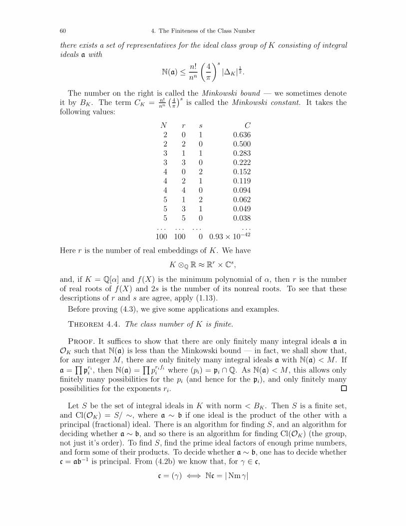
60 4. The Finiteness of the Class Number
there exists a set of representatives for the ideal class group of K consisting of integralideals a with
N(a) ≤ n!
nn
(4
π
)s
|∆K | 12 .
The number on the right is called the Minkowski bound — we sometimes denoteit by BK . The term CK = n!
nn
(4π
)sis called the Minkowski constant. It takes the
following values:
N r s C2 0 1 0.6362 2 0 0.5003 1 1 0.2833 3 0 0.2224 0 2 0.1524 2 1 0.1194 4 0 0.0945 1 2 0.0625 3 1 0.0495 5 0 0.038
. . . . . . . . . . . .100 100 0 0.93× 10−42
Here r is the number of real embeddings of K. We have
K ⊗Q R ≈ Rr × Cs,
and, if K = Q[α] and f(X) is the minimum polynomial of α, then r is the numberof real roots of f(X) and 2s is the number of its nonreal roots. To see that thesedescriptions of r and s are agree, apply (1.13).
Before proving (4.3), we give some applications and examples.
Theorem 4.4. The class number of K is finite.
Proof. It suffices to show that there are only finitely many integral ideals a inOK such that N(a) is less than the Minkowski bound — in fact, we shall show that,for any integer M , there are only finitely many integral ideals a with N(a) < M . If
a =∏
prii , then N(a) =
∏prifii where (pi) = pi ∩ Q. As N(a) < M , this allows only
finitely many possibilities for the pi (and hence for the pi), and only finitely manypossibilities for the exponents ri.
Let S be the set of integral ideals in K with norm < BK . Then S is a finite set,and Cl(OK) = S/ ∼, where a ∼ b if one ideal is the product of the other with aprincipal (fractional) ideal. There is an algorithm for finding S, and an algorithm fordeciding whether a ∼ b, and so there is an algorithm for finding Cl(OK) (the group,not just it’s order). To find S, find the prime ideal factors of enough prime numbers,and form some of their products. To decide whether a ∼ b, one has to decide whetherc = ab−1 is principal. From (4.2b) we know that, for γ ∈ c,
c = (γ) ⇐⇒ Nc = |Nmγ|
4. The Finiteness of the Class Number 61
and so we have to solve the equation:
Nm γ = constant.
When we express γ in terms of an integral basis, this becomes a (very special) typeof diophantine equation. For a description of an algorithm for finding Cl(OK), seePohst and Zassenhaus 1989, p424.
Example 4.5. Let K = Q[i]. The condition in the theorem is that N(a) ≤ 244π2 <
1.27. There are no such ideals other than Z[i], and so Z[i] is a principal ideal domain.(Of course, the elementary proof of this shows more, namely, that Z[i] is a Euclideandomain. Even for rings of integers in number fields, it is not true that all principalideal domains are Euclidean domains. For example, Q[
√−19] has class number 1,but its ring of integers is not a Euclidean domain. For more on such things, seethe survey article: Lemmermeyer, F., The Euclidean algorithm in algebraic numberfields, Exposition. Math., 13 (1995).)
Example 4.6. Let K = Q[√−5]. Here N(a) ≤ 0.63 × √20< 3. Any ideal
satisfying this must divide (2). In fact, (2) = p2 where p = (2, 1 +√−5), and
Np2 = N(2) = 4, and so Np = 2. The ideals OK and p form a set of representativesfor Cl(Z[
√−5]). The ideal p can’t be principal because there does not exist an ele-ment α = m+n
√−5 such that Nm(α) = m2+5n2 = 2, and so Cl(Z[√−5]) has order
2.
Example 4.7. Let K be a cubic field with discriminant < 0. Since the sign of ∆K
is (−1)s, and [K : Q] = r + 2s, we have s = 1, r = 1. The Minkowski bound is
B < 0.283|∆K | 12 .For |∆K| ≤ 49, B < 2, and so for cubic fields with −49 ≤ ∆K < 0, the class numberh = 1. For example, this is true for the number fields with discriminants −23 and−31 discussed earlier (see 2.35, 2.36).
For the field generated by a root of X3 + 10X + 1, the discriminant is −4027, andthe Minkowski bound is < 18. Recall from (3.49) that
(2) = (2, 1 + α)(2, 1 + α + α2).
Let p = (2, 1 + α)—its norm is 2. One can show that it generates the class group,and that it has order 6 in the class group, i.e., p6 but no smaller power is principal.Hence the class group is cyclic of order 6. (The proof takes quite a bit of hard workif you do it by hand — see Artin 1959, pp. 160-162, 170-172.)
An extension L of a number field K is said to be unramified over K if no primeideal of OK ramifies in OL.
Theorem 4.8. There does not exist an unramified extension of Q.
Proof. Let K be a finite extension of Q. Since a set of representatives for theclass group must have at least one element, and that element will have numericalnorm ≥ 1, Theorem 4.3 shows that
|∆| 12 ≥ nn
n!
(π
4
)s≥ nn
n!
(π
4
)n/2.
62 4. The Finiteness of the Class Number
Let an = rhs. Then a2 > 1, and an+1
an=
(π4
) 12 (1 + 1
n)n > 1, and so the sequence an is
monotonically increasing. Hence the discriminant of K has absolute value > 1, andwe know from (3.37) that any prime dividing the discriminant ramifies.
We can now prove that there is no irreducible monic polynomial f(X) ∈ Z[X] ofdegree > 1 with discriminant ±1. Let f(X) be such a polynomial, and let α be a root
of f(X). Then disc(Z[α]/Z) = ±1, and so Z[α] is the ring of integers in Kdf= Q[α]
and disc(OK/Z) = ±1, which we have just seen can’t happen.
Remark 4.9. There may exist unramified extensions of number fields other thanQ. In fact, class field theory says that the maximal abelian unramified11 extensionof K (called the Hilbert class field of K) has Galois group canonically isomorphic toCl(OK). For example, the theory says that Q[
√−5] has an unramified extension ofdegree 2, and one verifies that Q[
√−1,√−5] is unramified over Q[√−5].
Aside 4.10. Let K1 be a number field with class number hK1 > 1. Its Hilbertclass field is an abelian unramified extension K2 of K1 with Gal(K2/K1) ∼= Cl(K1).Let K3 be the Hilbert class field of K2, and so on. In this way, we obtain a tower offields,
K1 ⊂ K2 ⊂ K3 ⊂ · · ·It was a famous question (class field tower problem) to decide whether this towercan be infinite, or must always terminate with a field of class number 1 after a finitenumber of steps. It was shown by Golod and Shafarevich in the early 60s that thetower is frequently infinite. (See the article by Roquette in Cassels and Frohlich1967.)
Example 4.11. Let α be a root of f(X) = X5−X +1. As we saw in (2.38) thatf(X) is irreducible and its discriminant is 19 × 151, and so the ring of integers of
Kdf= Q[α] is Z[α].According to Theorem 4.3, every class of ideals for Q[α] contains an integral ideal
a with N(a) < 0.062 × √19× 151 = 3.3 < 4. If p is a prime ideal with N(p) = 2,then f(p/(2)) = 1, and f(X) must have a root mod 2, but it doesn’t, and so p can’texist. Similarly, there is no prime ideal p with N(p) = 3, and so OK is a principalideal domain!
The Galois group of the splitting field M of f(X) is S5 (later we shall see how tofind Galois groups; for the moment type “galois(X5−X +1);” in Maple), and hence[M : Q] = 120. It is possible to show that M is unramified over Q[
√19× 151].
Lattices. Let V be a vector space of dimension n over R. A lattice Λ in V is asubgroup of the form
Λ = Ze1 + · · ·+ Zer
with e1, ..., er linearly independent elements of V . Thus a lattice is the free abeliansubgroup of V generated by elements of V that are linearly independent over R.When r = n, the lattice is said to be full. At the opposite extreme, Λ = 0 is a
11The Hilbert class field L of K is required to be unramified even at the infinite primes — thismeans that every real embedding of K extends to a real embedding of L.
4. The Finiteness of the Class Number 63
lattice (generated by the empty set of elements). In terms of tensor products, onecan say that a full lattice in V is a subgroup Λ of V such that∑
ri ⊗ xi →∑
rixi, R⊗Z Λ→ V,
is an isomorphism.
Nonexample 4.12. The subgroup Z + Z√2 of R is a free abelian group of rank
2 (because√2 is not rational), but it is not a lattice in R.
We shall need another criterion for a subgroup Λ of V to be a lattice. The choiceof a basis for V determines an isomorphism of V with Rn, and hence a topology onV ; the topology is independent of the basis, because any linear automorphism of Rn
is a homeomorphism. A subgroup Λ of V is said to be discrete if it is discrete in theinduced topology. Recall that a topological space is discrete if its points (hence allsubsets) are open. Thus to say that Λ is discrete means that every point α of Λ hasa neighbourhood U in V such that U ∩ Λ = α.
Lemma 4.13. The following conditions on a subgroup Λ of a finite-dimensionalreal vector space V are equivalent:
(a) Λ is a discrete subgroup;(b) there is an open subset U of V such that U ∩ Λ = 0;(c) each compact subset of V intersects Λ in a finite set;(d) each bounded subset of V intersects Λ in a finite set.
Proof. (a) ⇐⇒ (b). Obviously (a) implies (b). For the converse, note that thetranslation map x → α + x : V → V is a homeomorphism, and that therefore if U isa neighbourhood of 0 such that U ∩ Λ = 0, then α + U is a neighbourhood of αsuch that (α+ U) ∩ Λ = α.
(a)⇒(c). Condition (a) says that Λ is a discrete space for the induced topology.Hence, if C is compact, then C ∩Λ is both discrete and compact, and therefore mustbe finite.
(c)⇒(d). The closure of a bounded set in Rn (hence in V ) is compact, and so thisis obvious.
(d)⇒(b). Let U be a bounded open neighbourhood of 0. Then S = U ∩ Λ 0is finite and hence closed, and so U S is an open neighbourhood of 0 such that(U S) ∩ Λ = 0.
Proposition 4.14. A subgroup Λ of V is a lattice if and only if it is discrete.
Proof. Clearly, a lattice is discrete. For the converse, let Λ be a discrete subgroupof V , and let e1, ..., er be a maximal R-linearly independent subset of Λ. We shall useinduction on r.
If r = 0, Λ = 0, and there is nothing to prove.
If r = 1, then every α ∈ Λ can be written α = ae1, some a ∈ R. Because Λ isdiscrete, ae1 | |a| < M ∩ Λ is finite, and so there is an f1 ∈ Λ such that, when wewrite f1 = ae1, a attains its minimum value > 0. I claim Λ = Zf1. If α ∈ Λ, α /∈ Zf1,then we can find an integer m such that α − mf1 = bf1 with 0 < b < 1; but then(α−mf1) = bf1 = abe1, and 0 < ab < a, which contradicts our choice of f1.
64 4. The Finiteness of the Class Number
Let Λ′ = Λ ∩ (Re1 + · · ·+ Rer−1). Clearly this is a discrete subgroup of the vectorspace V ′ =df Re1+ · · ·+Rer−1 and so, by induction, Λ′ = Zf1+ · · ·+Zfr−1 for somefi that are linearly independent over R (and hence also form a basis for V ′). Everyα ∈ Λ can be written uniquely
α = a1f1 + · · · + ar−1fr−1 + aer, ai, a ∈ R.
Let ϕ : Λ→ R be the map α → a, and let Λ′′ = Im(ϕ). Note that a is also the imageof
(a1 − [a1])f1 + · · ·+ (ar−1 − [ar−1])fr−1 + aer, [∗] = integer part,
and so each element a ∈ Λ′′ in a bounded set, say with 0 ≤ |a| < M , is the image ofan element of Λ in a bounded set,
0 ≤ ai < 1, i = 1, . . . , r − 1, |a| < M.
Thus there are only finitely many such a’s, and so Λ′′ is a lattice in R, say Λ′′ =Z · ϕ(fr), fr ∈ Λ.
Let α ∈ Λ. Then ϕ(α) = aϕ(fr) for some a ∈ Z, and ϕ(α − afr) = 0. Thereforeα− afr ∈ Λ′, and so it can be written
α − afr = a1f1 + · · ·+ ar−1fr−1, ai ∈ Z.
Hence
α = a1f1 + · · ·+ ar−1fr−1 + afr, ai, a ∈ Z,
which proves that Λ =∑
Zfi.
Let V be a real vector space of dimension n, and let Λ be a full lattice in V , sayΛ =
∑Zei. For any λ0 ∈ Λ, let
D = λ0 +∑
aiei | 0 ≤ ai < 1.Such a set is called a fundamental parallelopiped for Λ. The shape of the parallelopipeddepends on the choice of the basis (ei), but if we fix the basis and vary λ0 ∈ Λ, thenthe parallelopipeds cover Rn without overlaps.
Remark 4.15. (a) For a fundamental parallelopiped D of a full lattice
Λ = Zf1 + · · ·+ Zfn
in Rn, the volume of D
µ(D) = | det(f1, · · · , fn)|.(See any good book on calculus.) If also
Λ = Zf ′1 + Zf ′2 + · · · + Zf ′n,
then the determinant of the matrix relating fi and f ′i has determinant ±1, andso the volume of the fundamental parallelopiped doesn’t depend on the choice of thebasis for Λ.
(b) When Λ ⊃ Λ′ are two full lattices Rn, we can choose bases ei and fi forΛ and Λ′ such that fi = miei with mi a positive integer. With this choice of bases,
4. The Finiteness of the Class Number 65
the fundamental parallelopiped D of Λ is a disjoint union of (Λ : Λ′) fundamentalparallelopipeds D′ of Λ′. Hence
µ(D′)µ(D)
= (Λ : Λ′) (*).
As we noted above, the choice of a basis for V determines an isomorphism V ≈ Rn,and hence a measure µ on V . This measure is translation invariant (because theLebesgue measure on Rn is translation invariant), and well-defined up to multiplica-tion by a nonzero constant (depending on the choice of the basis) 12. Thus the ratioof the measures of two sets is well-defined, and the equation (*) holds for two fulllattices Λ ⊃ Λ′ in V .
Theorem 4.16. Let D0 be a fundamental parallelopiped for a full lattice in V , andlet S be a measurable subset in V . If µ(S) > µ(D0), then S contains distinct pointsα and β such that β − α ∈ Λ.
Proof. The set S ∩D is measurable for all fundamental parallelopipeds D, and
µ(S) =∑
µ(S ∩D)
(sum over translates of D by elements of Λ). For each D, a (unique) translate ofS ∩D by an element of Λ will be a subset of D0. Since µ(S) > µ(D0), at least two ofthese sets will overlap, i.e., there exist elements α, β ∈ S such that
α − λ = β − λ′, some λ, λ′ ∈ Λ.
Then β − α ∈ Λ.
Remark 4.17. In the language of differential geometry, the theorem can be givena more geometric statement. Let M = V/Λ; it is an n-dimensional torus. Themeasure µ on V defines a measure on M for which M has measure µ(M) = µ(D).The theorem says that if µ(S) > µ(M), then the restriction of the quotient mapV → M to S can’t be injective.
Let T be a set such that
α,β ∈ T ⇒ 1
2(α− β) ∈ T, (*)
and let S = 12T . Then T contains the difference of any two points of S, and so T will
contain a point of Λ other than the origin whenever
µ(D) < µ(1
2T ) = 2−nµ(T ),
i.e., whenever
µ(T ) > 2nµ(D).
We say that a set T is convex if, with any two points, it contains the line joiningthe two points, and that T is symmetric in the origin if α ∈ T implies −α ∈ T . Aconvex set, symmetric in the origin, obviously satisfies (*), and so it will contain apoint of Λ \ 0 if its volume is greater than 2nµ(D).
12The experts will recognize µ as being a Haar measure on V .
66 4. The Finiteness of the Class Number
Theorem 4.18 (Minkowski’s). Let T be a subset of V that is compact, convex,and symmetric in the origin. If
µ(T ) ≥ 2nµ(D)
then T contains a point of the lattice other than the origin.
Proof. Replace T with (1+ε)T , ε > 0. Then µ((1+ε)T ) = (1+ε)nµ(T ) > 2nµ(D),and so (1+ε)T contains a point of Λ other than the origin (see the preceding remark).It will contain only finitely many such points because Λ is discrete and (1 + ε)T iscompact. Because T is closed
T = ∩ε>0(1 + ε)T.
If none of the points of Λ ∩ (1 + ε)T is in T , we will be able to shrink (1 + ε)T(keeping ε > 0) so that it contains no point of Λ other than the origin—which is acontradiction.
Remark 4.19. Theorem 4.18 was discovered by Minkowski in 1896. Although itis almost trivial to prove, it has lots of nontrivial consequences, and was the startingpoint for the branch of number theory (now almost defunct) called the “geometryof numbers”. We give one immediate application of it to prove that every positiveinteger is a sum of four squares of integers.
From the identity
(a2 + b2+ c2 + d2)(A2 +B2 + C2 +D2) =
(aA− bB − cC − dD)2 + (aB + bA + cD − dC)2 +
(aC − bD + cA + dB)2 + (aD + bC − cB + dA)2,
we see that it suffices to prove that a prime p is a sum of four squares.
Since
2 = 12 + 12 + 02 + 02,
we can suppose that p is odd. I claim that the congruence
m2 + n2 + 1 ≡ 0 mod p
has a solution in Z. As m runs through 0, 1, . . . , p − 1, m2 takes exactly (p + 1)/2distinct values modulo p, and similarly for −1− n2. For the congruence to have nosolution, all these values, p+ 1 in total, must be distinct, but this is impossible.
Fix a solution m,n to the congruence, and consider the lattice Λ ⊂ Z4 consistingof (a, b, c, d) such that
c ≡ ma+ nb, d ≡ mb− na mod p.
Then Z4 ⊃ Λ ⊃ pZ4 and Λ/pZ4 is a 2-dimensional subspace of F4p (the a and b can be
arbitrary mod p, but then c and d are determined). Hence Λ has index p2 in Z4, andso the volume of a fundamental parallelopiped is p2. Let T be a closed ball of radiusr centered at the origin. Then T has volume π2r4/2, and so if we choose r2 > 1.9psay, then
µ(T ) > 16µ(D).
4. The Finiteness of the Class Number 67
According to Minkowski’s theorem, there is a point (a, b, c, d) ∈ (Λ\0)∩T . Because(a, b, c, d) ∈ Λ,
a2 + b2 + c2 + d2 ≡ a2(1 +m2 + n2) + b2(1 +m2 + n2) ≡ 0 mod p,
and because (a, b, c, d) ∈ T ,
a2 + b2 + c2 + d2 < 2p.
As a2 + b2 + c2 + d2 is a positive integer, these conditions imply that it equals p.
This result was stated by Fermat. Euler tried to prove it over a period of 40 years,and Lagrange succeeded in 1770.
Some calculus. Let V be a finite-dimensional real vector space. A norm on V is afunction ‖ · ‖ : V → R such that
(4.20.1) for all x ∈ V , ‖x‖ ≥ 0, and ‖x‖ = 0 ⇐⇒ x = 0;(4.20.2) for r ∈ R and x ∈ V , ‖rx‖ = |r|‖x‖;(4.20.3) (triangle law) for x,y ∈ V , ‖x+ y‖ ≤ ‖x‖+ ‖y‖.
Let V = Rr × Cs — it is a real vector space of dimension n = r + 2s. Define anorm on V by
‖x‖ =r∑i=1
|xi|+ 2s∑
i=r+1
|zi|
if x = (x1, ..., xr, zr+1, ..., zr+s).
Lemma 4.21. For any real number t > 0, let
X(t) = x ∈ V | ‖x‖ ≤ t.Then
µ(X(t)) = 2r(π/2)stn/n!.
Proof. Since X(t) is symmetric with respect to the r real axes, we have
µ(X(t)) = 2r · µ(Y (t))
where Y (t) = x | ‖x‖ ≤ t, x1, ..., xr ≥ 0. For the complex variables, we make thechange of variable
zj = xj + iyj =1
2ρj(cos θj + i sin θj).
The Jacobian of this change of variables is ρj/4. After integrating over the θj, for0 ≤ θj ≤ 2π, we find that
µ(X(t)) = 2r · 4−s · (2π)s∫Z
ρr+1 · · · ρr+sdx1 · · · dxrdρr+1 · · · dρr+swhere
Z = (x, ρ) ∈ Rr+s | xi, ρi ≥ 0,∑
xi +∑
ρi ≤ t.The result now follows from the next lemma by taking: m = r+ s; ai = 0, 1 ≤ i ≤ r;ai = 1, r + 1 ≤ i ≤ m; for then
µ(X(t)) = 2r · 4−s · (2π)s · tn/n!as required.
68 4. The Finiteness of the Class Number
Lemma 4.22. For ai > 0 ∈ R, let
I(a1, ..., am, t) =
∫Z(t)
xa11 · · ·xam
m dx1 · · · dxm,
where Z(t) = x ∈ Rm | xi ≥ 0,∑
xi ≤ t. Then
I(a1, . . . , am; t) = t∑ai+m · Γ(a1 + 1) · · ·Γ(am + 1)
Γ(a1 + · · ·+ am +m+ 1).
Proof. Recall that, by definition, (e.g., Widder, D., Advanced Calculus, 1961,Chapter 11),
Γ(x) =
∫ ∞
0+
e−ttx−1dt.
It takes the value Γ(n) = (n− 1)! for n a nonnegative integer.
By making the change of variables x′i = txi in I , we see that
I(a1, . . . , am; t) = t∑ai+mI(a1, . . . , am; 1).
Therefore it suffices to prove the formula for t = 1. We prove this case by inductionon m. First, we have
I(a1; 1) =
∫ 1
0
xa11 dx1 =
1
a1 + 1=
Γ(a1 + 1)
Γ(a1 + 2).
Let
Z(xm)′ = x ∈ Rm−1 | xi ≥ 0,
∑xi ≤ 1− xm.
Then
I(a1, ..., am; 1) =
∫ 1
0
xamm
(∫Z(xm)′
xa11 · · ·xam−1
m−1 dx1 · · · dxm−1)dxm,
=
∫ 1
0
xamm I(a1, ..., am−1; 1− xm)dxm
= I(a1, ..., am−1; 1)∫ 1
0
xamm (1− xm)
∑ai+m−1dxm
= I(a1, ..., am−1; 1)Γ(am + 1)Γ(a1 + · · ·+ am−1 +m)
Γ(a1 + · · ·+ am +m+ 1).
In the last step, we used the standard formula∫ 1
0
xm−1(1− x)n−1dx = B(m,n) =Γ(m)Γ(n)
Γ(m + n).
Example 4.23. (a) Case r = 2, s = 0. Then X(t) is defined by |x|+ |y| ≤ t. It isa square of side
√2t, and so µ(X(t)) = 2t2.
(b) Case r = 0, s = 1. Then X(t) is the circle of radius t/2, which has area πt2/4.
4. The Finiteness of the Class Number 69
Lemma 4.24. Let a1, . . . , an be positive real numbers. Then
(∏
ai)1/n ≤ (
∑ai)/n;
equivalently, ∏ai ≤ (
∑ai)
n/nn.
(The geometric mean is less than or equal to the arithmetic mean.)
Proof. See any good course on advanced calculus.
Finiteness of the class number. Let K be number field of degree n over Q.Suppose that K has r real embeddings σ1, . . . , σr and 2s complex embeddingσr+1, σr+1, . . . , σr+s, σr+s. Thus n = r + 2s. We have an embedding
σ : K → Rr ×Cs, α → (σ1α, . . . , σr+sα).
We identify Vdf= Rr × Cs with Rn using the basis 1, i for C.
Proposition 4.25. Let a be an ideal in OK; then σ(a) is a full lattice in V , and
the volume of a fundamental parallelopiped of σ(a) is 2−s · Na · |∆K| 12 .Proof. Let α1, . . . , αn be a basis for a as a Z-module. To prove that σ(a) is a
lattice we show that the vectors σ(α1), . . . , σ(αn) are linearly independent, and weprove this by showing that the matrix A, whose ith row is
(σ1(αi), . . . , σr(αi),&(σr+1αi),'(σr+1αi), . . . )
has nonzero determinant.
First consider the matrix B whose ith row is
(σ1(αi), . . . , σr(αi), σr+1(αi), σr+1(αi), . . . , σr+s(αi)).
We saw in (2.25) that det(B)2 = disc(α1, . . . , αn) = 0.
What is the relation between the determinants of A and B? Add column r + 2 inB to column r+1, and then subtract 1/2 column r+1 from column r+2. This givesus 2&(σr+1(αi)) in column r + 1 and −i'(σr+1(αi)) in column r + 2. Repeat for theother pairs of columns. These column operations don’t change the determinant of B,and so
det(B) = (−2i)s det(A),
or
det(A) = (−2i)−s det(B) = (−2i)−s disc(α1, . . . , αn)1/2 = 0.
Thus σ(a) is a lattice in V.
Since σ(a) =∑n
i=1 Zσ(αi), the volume of a fundamental parallelopiped D for σ(a)is | det(A)|, and from (2.24) we know that
| disc(α1, . . . , αn)| = (OK : a)2 · | disc(OK/Z)|.Hence
µ(D) = 2−s · | disc(α1, . . . , αn)| 12 = 2−s · Na · |∆K | 12 .
70 4. The Finiteness of the Class Number
Proposition 4.26. Let a be an ideal in OK. Then a contains a nonzero elementα of K with
|Nm(α)| ≤ BK · Na =
(4
π
)sn!
nnNa|∆| 12 .
Proof. Let X(t) be as in (4.21), and letD be a fundamental domain for the latticeσ(a). The set X(t) is compact convex and symmetric in the origin, and so, when wechoose t so large that µ(X(t)) ≥ 2n · µ(D), Minkowski’s Theorem shows that X(t)contains a point σ(α) = 0 of σ(a). For this α ∈ a,
|Nm(α)| = |σ1(α)| · · · |σr(α)||σr+1(α)|2 · · · |σr+s(α)|2≤ (
∑|σiα| +
∑2|σiα|)n/nn (by 4.24)
≤ tn/nn.
In order to have µ(X(t)) ≥ 2n · µ(D), we need
2r(π/2)stn/n! ≥ 2n · 2−s · Na · |∆K | 12 ,i.e.,
tn ≥ n! · 2n−r
πs· Na · |∆K | 12 .
When we take tn to equal the expression on the right, we find that
|Nm(α)| ≤ n!
nn· 2
n−r
πs· Na · |∆K| 12 .
As n− r = 2s, this is the required formula.
Proof of Theorem 4.3. Let c be a fractional ideal in K — we have to showthat the class of c in the ideal class group is represented by an integral ideal a with
Na ≤ BKdf=
n!
nn
(4
π
)s
|∆K| 12 .
For some d ∈ K×, dc−1 is an integral ideal, say (d) · c−1 = b. According to the resultjust proved, there is a β ∈ b, β = 0, with
|Nm(β)| ≤ BK · Nb.
Now βOK ⊂ b⇒ βOK = ab with a integral, and a ∼ b−1 ∼ c. Moreover,
Na · Nb = |NmL/K β| ≤ BK · Nb.
On cancelling Nb, we find that Na ≤ B.
Remark 4.27. Proposition 4.26 can be useful in deciding whether an integral idealis principal.
4. The Finiteness of the Class Number 71
Binary quadratic forms. The first person to consider class numbers (implicitly)was Gauss. Rather than working with ideals, which hadn’t been defined then, heworked with binary quadratic forms.
By a binary quadratic form we mean an expression of the form
Q(X, Y ) = aX2 + bXY + cY 2.
We call the form integral if Q(m,n) is an integer whenever m and n are integers, or,equivalently, if a, b, c ∈ Z. The discriminant of Q is
dQ = b2 − 4ac.
A form is said to be nondegenerate if its discriminant is nonzero. Two integralbinary quadratic forms Q and Q′ are said to be equivalent if there exists a matrix
A =
(α βγ δ
)∈ SL2(Z) such that
Q′(X, Y ) = Q(αX + βY, γX + δY ).
Clearly, equivalent forms have the same discriminant, but there exist inequivalentforms with the same discriminant. The question considered by Gauss was to try todescribe the set of equivalence classes of forms with a fixed discriminant. As we shallexplain, this question can be interpreted in terms of ideals.
Let d = 1 be a square-free integer, let K = Q[√d], and let dK = disc(OK/Z).
Define the norm form qK by
qK(X, Y ) = NmK/Q(X + Y√d) = X2 − dY 2, if d ≡ 2, 3 mod 4
or
qK(X, Y ) = NmK/Q(X + Y1 +√d
2) = X2 +XY +
1− d
4Y 2, if d ≡ 1 mod 4.
In both cases qK has discriminant dK (= 4d or d).
In general, if Q is an integral binary quadratic form, then dQ = dKf2, some integer
f , where K = Q[√
dQ]. Moreover, if dQ = dK , then Q is primitive, i.e., gcd(a, b, c) =1.
Fix a field K = Q[√d] and an embedding K → C. We choose
√d to be positive if
d > 0 and to have positive imaginary part if d is negative. Set√dK = 2
√d or√d.
Write Gal(K/Q) = 1, σ. If d < 0, define Cl+(K) = Cl(K) (usual class group of K)and if d > 0, define
Cl+(K) = Id(K)/P+(K)
where P+(K) is the group of principal ideals of the form (α) with α > 0 under everyembedding of K into R.
Let a be a fractional ideal in K, and let a1, a2 be a basis for a as a Z-module. From(2.24) we know that ∣∣∣∣ a1 a2
σa1 σa2
∣∣∣∣2
= dKNa2.
72 4. The Finiteness of the Class Number
After possibly reordering the pair a1, a2 we will have∣∣∣∣ a1 a2σa1 σa2
∣∣∣∣ =√
dKNa.
For such a pair, define
Qa1,a2(X, Y ) = Na−1 · NmK/Q(a1X + a2Y ).
This is an integral binary quadratic form with discriminant dK .
Theorem 4.28. The equivalence class of Qa1,a2(X, Y ) depends only on the imageof a in Cl+(K); moreover, the map sending a to the equivalence class of Qa1,a2 definesa bijection from Cl+(K) to the set of equivalence classes of integral binary quadraticforms with discriminant dK .
Proof. See Frohlich and Taylor 1991, VII.2 (and elsewhere).
In particular, the set of equivalence classes is finite, and has the structure of anabelian group. This was known to Gauss, even though groups had not yet beendefined. (Gauss even knew it was a direct sum of cyclic groups.)
Remark 4.29. Write hd for the class number of Q[√d], d a square-free integer = 1.
In modern terminology, Gauss conjectured that, for a fixed h, there are only finitelymany negative d such that hd = h. (Actually, because of a difference of terminology,this is not quite what Gauss conjectured.)
In 1935, Siegel showed that, for every ε > 0, there exists a constant c > 0 such that
hd > c|d| 12−ε, d < 0.
This proves Gauss’s conjecture. Unfortunately, the c in Siegel’s theorem is not effec-tively computable, and so Siegel’s theorem gives no way of computing the d’s for agiven h.
In 1951, Tatuzawa showed that Siegel’s theorem is true with an effectively com-putable c except for at most one exceptional d.
It is easy to show that hd = 1 for −d = 1, 2, 3, 7, 11, 19, 43, 67, 163 (exercise!). Thusin 1951 it was known that there exist these 9 quadratic imaginary number fields withclass number 1, and possibly 1 more.
In 1952 Heegner proved that there was no 10th such field, but his proof was notrecognized to be correct for many years.
More recently (1983), Goldfeld, Gross, and Zagier showed, using completely differ-ent methods from Siegel, that there is an effective procedure for finding all d < 0 withhd equal to a given h. For an expository article on this, see Goldfeld, Bull. Amer.Math. Soc. 13 (1985), 23–37.
By way of contrast, it is conjectured that there are infinitely many real quadraticfields with class number 1, but this has not been proved.
There are tables of class numbers at the back of Borevich and Shafarevich 1966(and elsewhere).
5.The Unit Theorem 73
5. The Unit Theorem
In this section we prove the second main theorem of the course.
Statement of the theorem. Recall that a finitely generated abelian group A isisomorphic to Ators ⊕ Zr for some r where Ators is the (finite) subgroup of torsionelements of A (i.e., of elements of finite order). The number r is uniquely determinedby A, and is called the rank of A.
Theorem 5.1. The group of units in a number field K is finitely generated withrank equal to r + s− 1.
The theorem is usually referred to as the “Dirichlet Unit Theorem” although Dirich-let in fact proved it for rings of the form Z[α] rather than OK.
Write UK (= O×K) for the group of units in K. The torsion subgroup of UK is(obviously) the group µ(K) of roots of 1 in K.
A set of units u1, . . . , ur+s−1 is called a fundamental system of units if it forms abasis for UK modulo torsion, i.e., if every unit u can be written uniquely in the form
u = ζum11 · · ·umr+s−1
r+s−1 , ζ ∈ µ(K), mi ∈ Z.
The theorem implies that µ(K) is finite (and hence cyclic). This can be proveddirectly. In §7, we shall see that, if ζm is a primitive mth root of 1, then Q[ζ] is aGalois extension of Q with Galois group isomorphic to (Z/mZ)×. Note that
#(Z/mZ)× = #n | 0 ≤ n ≤ m− 1, gcd(n,m) = 1df= ϕ(m) (Euler ϕ-function)
and
ϕ(m) =∏
ϕ(prii ) =
∏pri−1i (pi − 1), for m =
∏prii ,
which increases with m. Since
ζm ∈ K ⇒ Q[ζm] ⊂ K ⇒ ϕ(m)|[K : Q],
this implies that µ(K) is finite.
Lemma 5.2. An element α ∈ K is a unit if and only if α ∈ OK and NmK/Q α =±1.
Proof. If α is a unit, then there is a β ∈ OK such that αβ = 1, and then Nm(α)and Nm(β) lie in Z and 1 = Nm(αβ) = Nm(α) · Nm(β). Hence Nmα ∈ Z× = ±1.
For the converse, fix an embedding σ0 of K into C, and use it to identify K witha subfield of C. Recall (2.19) that
Nmα =∏σ
σα = α ·∏σ =σ0
σα, σ : K → C.
Let β =∏
σ =σ0σα. If α ∈ OK then β is an algebraic integer. If Nmα = ±1, then
β = ±α−1 and so belongs to K. Therefore, if α satisfies both conditions, it has aninverse ±β in OK , and so is a unit.
For all real fields, i.e., fields with an embedding into R, µ(K) = ±1; for “most”nonreal fields, this is also true.
74 5. The Unit Theorem
Example 5.3. Let K be a quadratic field Q[√d]. Then OK = m+n
√d | m,n ∈
Z or m + n(1 +√d)/2 | m,n ∈ Z. The units in K are given by the solutions of
the equation:
m2 − n2d = ±1, or (2m+ n)2 − dn2 = 4.
When d < 0, these equations (obviously) have only finitely many solutions, and soUK = µ(K). Note that ζm lies in a quadratic field if and only if ϕ(m) ≤ 2. This onlyhappens for m dividing 4 or 6. Thus µ(K) = ±1 except for the following fields:
Q[i], µ(K) = ±1,±i;Q[√−3], µ(K) = ±1,±ρ,±ρ2, with ρ = (1 +
√−3)/2).When d > 0, the theorem shows that there are infinitely many solutions, and thatUK = ±uZ for some element u (called the fundamental unit). As H. Cohn (A ClassicalInvitation...) puts it, “the actual computation of quadratic units lies in the realm ofpopularized elementary number theory, including devices such as continued fractions.”The method is surprisingly effective, and yields some remarkably large numbers —see later.
Example 5.4. Let K = Q[α], where α is a root of X3 + 10X + 1. We know thatthe discriminant ∆K = −4027. Since sign(∆K) = (−1)s and r+2s = 3, we must haver = 1 = s. From its minimum equation, we see that Nmα = −1, and so α is a unit.Later we shall show that α is a fundamental unit, and so UK = ±αm | m ∈ Z.Proof that UK is finitely generated. We first need a simple lemma.
Lemma 5.5. For any integers m and M , the set of all algebraic integers α suchthat
(i) the degree of α is ≤ m, and
(ii) |α′| < M for all conjugates α′ of αis finite.
Proof. The first condition says that α is a root of a monic irreducible polynomialof degree≤ m, and the second condition implies that the coefficients of the polynomialare bounded. Since the coefficients are integers, there are only finitely many suchpolynomials, and hence only finitely many α’s.
Recall that we previously considered the map
σ : K → Rr ×Cs, α → (σ1α, . . . , σrα, σr+1α, . . . , σr+sα)
where σ1, . . . , σr, σr+1, σr+1, . . . , σr+s, σr+s is the complete set of embeddings of Kinto C. It takes sums to sums. Now we want a map that takes products to sums, andso we take logarithms. Thus we consider the map:
L : K× → Rr+s, α → (log |σ1α|, . . . , log |σrα|, 2 log |σr+1α|, . . . , 2 log |σr+sα|).It is a homomorphism. If u is a unit in OK , then NmK/Q u = ±1, i.e.,
|σ1α| · · · |σrα||σr+1α|2 · · · |σr+sα|2 = 1.
On taking logs, we see that L(u) is contained in the hyperplane
H : x1 + · · ·+ xr + 2xr+1 + · · ·+ 2xr+s = 0.
5.The Unit Theorem 75
Dropping the last coordinate defines an isomorphism H ≈ Rr+s−1.
Proposition 5.6. The image of L : U → H is a lattice in H, and the kernel of Lis a finite group (hence is µ(K)).
Proof. Let C be a bounded subset of H containing 0, say
C ⊂ x ∈ H | |xi| ≤ M.If L(u) ∈ C , then |σju| ≤ eM for all j, and Lemma 5.5 implies that there are onlyfinitely many such u’s. Thus L(U)∩C is finite, and this implies that L(U) is a latticein H (by 4.14). Since everything in the kernel maps into C , the kernel is finite.
Since the kernel of L is finite, we have
rank(U) = rank(L(U)) ≤ dimH = r + s− 1.
Computation of the rank. We now prove the unit theorem.
Theorem 5.7. The image L(U) of U in H is a full lattice; thus U has rank r+s−1.Proof. To prove the theorem, we have to find a way to construct units. We work
again with the embedding
σ : K → Rr × Cs ≈ Rr+2s.
For x = (x1, ..., xr, xr+1, ...) ∈ Rr × Cs, define
Nm(x) = x1 · · · xr · xr+1 · xr+1 · · ·xr+s · xr+s.Then Nm(σ(α)) = Nm(α). Note that |Nm(x)| = |x1| · · · |xr||xr+1|2 · · · |xr+s|2.
Recall from (4.25), that σ(OK) is a full lattice in Rr × Cs, and the volume of its
fundamental parallelopiped is 2−s · |∆| 12 ; in more detail, if α1, . . . , αn is a Z-basis forOK , then we showed that the absolute value of the determinant of the matrix whoseith row is
σ(αi) = (σ1(αi), . . . ,&(σr+1(αi)),'(σr+1(αi)), . . . )
is 2−s · |∆| 12 . In fact, we showed that we could get this matrix from the matrix whoseith row is
(σ1(αi), . . . , σr+1(αi), σr+1(αi), . . . )
by some elementary column operations that multiplied the absolute value of thedeterminant by 2−s, and we know that the determinant of the second matrix is ±|∆| 12 .
In the rest of the proof, x will be a point of Rr × Cs with
1/2 ≤ |Nm(x)| ≤ 1.
Define
x · σ(OK) = x · σ(α) | α ∈ OK.Since Rr × Cs is a ring, this product makes sense. This is again a lattice in Rr ×Cs,and the volume of its fundamental parallelopiped is the determinant of the matrixwhose ith row is
(x1σ1(αi), . . . ,&(xr+1σr+1(αi)),'(xr+1σr+1(αi)), . . . ).
76 5. The Unit Theorem
As before, the absolute value of the determinant of this matrix is 2−s times theabsolute value of the determinant of the matrix whose ith row is
(x1σ1(αi), . . . , xr+1 · σr+1(αi), xr+1 · σr+1(αi), . . . ),
which is
|∆| 12 · |Nm(x)|.Therefore x ·σ(OK) is a lattice with 2−s|∆| 12 |Nm(x)| as the volume of its fundamentaldomain. Note that as x ranges over our set these volumes remain bounded.
Let T be a compact convex subset of Rr × Cs, which is symmetric in the origin,and whose volume is so large that, for every x in the above set, Minkowski’s theorem(4.18) implies there is a point γ of OK , γ = 0, such that x · σ(γ) ∈ T . The points ofT have bounded coordinates, and hence bounded norms, and so
x · σ(γ) ∈ T ⇒ |Nm(x · σ(γ))| ≤ M,
for some M (depending on T ); thus
|Nm(γ)| ≤M/Nm(x) ≤ 2M.
Consider the set of ideals γ · OK , where γ runs through the γ’s in OK for whichx · σ(γ) ∈ T for some x in our set. The norm N of such an ideal is ≤ 2M , and sothere can only be finitely many such ideals, say γ1 · OK, . . . , γt · OK . Now if γ is anyelement of OK with x · σ(γ) ∈ T , some x, then γ · OK = γi · OK for some i, andso there exists a unit ε such that γ = γi · ε. Then x · σ(ε) ∈ σ(γ−1i ) · T . The setT ′ = σ(γ−11 ) · T ∪ ... ∪ σ(γ−1t ) · T is bounded, and so we have shown that, for eachx in our set there exists a unit ε such that the coordinates of x · σ(ε) are boundeduniformly in x (the set T ′ doesn’t depend on x).
We are now ready to prove that L(U) is a full lattice in H. If r + s− 1 = 0, thereis nothing to prove, and so we assume r + s− 1 ≥ 1.
For each i, 1 ≤ i ≤ r + s, we choose an x in our set such that all the coordinatesof x except xi are very large (compared with T ′), and xi is sufficiently small that|Nmx| = 1. We know that there exists a unit εi such that x · σ(εi) has boundedcoordinates, and we deduce that |σjεi| < 1 for j = i, and hence that log |σjεi| < 0.
I claim that L(ε1), ..., L(εr+s−1) are linearly independent vectors in the lattice L(U).For this we have to prove that the matrix whose ith row is
(l1(εi), ..., lr+s−1(εi)), li(ε) = log |σiε|,is invertible. The elements of the matrix except those on the diagonal are negative,but the sum
l1(εi) + · · ·+ lr+s−1(εi) + lr+s(εi) = 0,
and so the sum of the terms in the ith row
l1(εi) + · · ·+ lr+s−1(εi) = −lr+s(εi) > 0.
The next lemma implies that the matrix is invertible, and so completes the proof ofTheorem 5.7.
Lemma 5.8. Let (aij) be a real m×m matrix such that
(a) aij < 0 for i = j;
5.The Unit Theorem 77
(b)∑
j aij > 0 for i = 1, 2, ..., m.
Then (aij) is invertible.
Proof. If it isn’t, then the system of equations∑aijxj = 0
has a nontrivial solution. Write x1, ..., xm for such a solution, and suppose i is suchthat |xi| = max|xj|. We can scale the solution so that xi = 1. Then |xj| ≤ 1 forj = i, and the ith equation is
0 =∑
aijxj = aii +∑j =i
aijxj ≥ aii +∑j =i
aij > 0.
S-units. Let S be a finite set of prime ideals of K, and define the ring of S-integersto be
OK(S) = ∩p/∈SOp = α ∈ K | ordp(α) ≥ 0, all p /∈ S.For example, if S = ∅, then OK(S) = OK .
Define the group of S-units, to be
U(S) = OK(S)× = α ∈ K | ordp(α) = 0, all p /∈ S.Clearly, the torsion subgroup of U(S) is again µ(K).
Theorem 5.9. The group of S-units is finitely generated with rank r+s+#S−1.Proof. Let p1, p2, . . . , pt be the elements of S. The homomorphism
u → (. . . , ordpi(u), . . . ) : U(S)→ Zt
obviously has kernel U . To complete the proof, it suffices to show that the image ofU(S) in Zt has rank t. Let h be the class number of K. Then phi is principal, sayphi = (πi), and πi is an S-unit with image
(0, . . . , h, . . . , 0) (h in the ith position).
Clearly these elements generate a subgroup of rank t.
For example, if K = Q and S = (2), (3), (5) thenU(S) = ±2k3m5n | k,m, n ∈ Z,
and the statement is obvious in this case.
Finding fundamental units in real quadratic fields. An expression
a0 +1
a1 +1
a2 +1
a3 + . . .
is called a continued fraction. We abbreviate the expression on the right as
[a0, a1, a2, . . . ].
78 5. The Unit Theorem
We shall always assume that the ai are integers with a1 > 0, a2 > 0, . . . . Theintegers ai are called the quotients, and [a0, a1, ..., an] is called the nth convergent.Every irrational number α can be expressed in just one way as an infinite continuedfraction, and the continued fraction is periodic if and only if α has degree 2 over Q.(See any book on elementary number theory, for example, Hardy, G. H., and Wright,E. M., An Introduction to the Theory of Numbers, Oxford Univ. Press, 1960 (4thedition), Chapter X.)
Now let d be a square-free positive integer, and let ε be the (unique) fundamental
unit for Q[√d] with ε > 1. Let s be the period of the continued fraction for
√d and
let p/q be the (s− 1)th convergent of it; then
ε = p + q√d if d ≡ 2, 3 mod 4, or d ≡ 1 mod 8,
and
ε = p + q√d or ε3 = p+ q
√d otherwise.
Using Maple or Mathematica, it is very easy to carry this out, and one obtains somespectacularly large numbers.
For example, to find the fundamental unit in Q[√
94], first compute√94 = 9.
6954 . . . . Then compute the continued fraction of√94. One gets
9, 1, 2, 3, 1, 1, 5, 1, 8, 1, 5, 1, 1, 3, 2, 1, 18, 1, 2, 3, . . . .This suggests the period is 16. Now evaluate the 15th convergent. One gets
2143295
221064
Hence the fundamental unit > 1 is
ε = 2143295 + 221064 · √94.Compute that
(2143295)2 − (221064)2 · 94 = 1,
which verifies that ε is a unit.
When one carries out this procedure for Q[√
9199], the first coefficient of the fun-damental unit has 88 digits! The computer has no problem finding the fundamentalunit — the only problem is counting the length of the period, which is about 180.
Units in cubic fields with negative discriminant. Since the sign of the discrim-inant is (−1)s (see 2.39), a cubic field K will have negative discriminant if and onlyif r = 1 = s. We identify K with a subfield of R using its unique real embedding.We have ∆ < 0, and the group of units is ±εm for some ε (fundamental unit). Wewant to find ε. Since -ε, −ε−1, and ε−1 are also fundamental units, we may supposethat ε > 1.
Lemma 5.10. Let K be a cubic extension of Q with negative discriminant, and letε be the fundamental unit with ε > 1. Then
|∆K | < 4ε3 + 24.
5.The Unit Theorem 79
Proof. Since ε /∈ Q, it must generate K. The two conjugates of ε (other than εitself) must be complex conjugates, and so the product of ε with its conjugates mustbe +1 (rather than −1). Write ε = u2, u ∈ R, u > 1. Then the remaining conjugatesof ε can be written
u−1eiθ, u−1e−iθ (0 ≤ θ ≤ π).
Let ∆′ = D(1, ε, ε2) be the discriminant of the minimum equation of ε. Then
∆′12 = (u2 − u−1eiθ)(u2 − u−1e−iθ)(u−1eiθ − u−1e−iθ) = 2i(u3 + u−3 − 2 cos θ) sin θ.
If we set 2ξ = u3 + u−3, then
|∆′| 12 = 4(ξ − cos θ) sin θ,
which, for a given u, has a maximum where
ξ cos θ − cos2 θ + sin2 θ = 0,
or
−g(x) df= ξx − 2x2 + 1 = 0, |x| ≤ 1, x = cos θ.
We seek a root of g(x) with |x| < 1. But g(1) = 1 − ξ < 0 (because u > 1 implies
ξ = u3−u−3
2> 1), and g(− 1
2u3 ) =34(u−6 − 1) < 0. Since g(x) = 2x2 + · · · , it follows
g(x) has one root > 1, and that the desired root x0, with |x0| ≤ 1, is < − 12u3 . But
then
x20 >1
4u6⇒ u−6 − 4x20 < 0⇒ u−6 − 4x−20 − 4x40 < 0. (*)
This maximum yields
|∆′| ≤ 16(ξ2 − 2ξx0 + x20)(1− x20),
and, on applying the conditions ξx0 = 2x20−1, ξ2x20 = 4x40−4x20+1, and the inequality(*) we find that
|∆′| ≤ 16(ξ2 + 1− x20 − x40) = 4u6 + 24 + 4(u−6 − 4x20 − 4x40) < 4u6 + 24.
Hence
|∆′| < 4ε3 + 24.
Since ∆′ = ∆K · (square of an integer), this completes the proof.
Example 5.11. Let K = Q[α] where α is a real root of X3 + 10X + 1. Here the
discriminant is −4027, and so ε > 3
√4027−24
4> 10 for ε the fundamental unit with
ε > 1. Note that Nm(α) = −1, and so α is a unit. Moreover, α = −0.0999003... andso β = −α−1 = 10.00998.... Since β is a power of ε, we must have β = ε; i.e., −α−1is the fundamental unit > 1. Thus
UK = ±αm | m ∈ Z.Once one knows ε, it becomes easier to compute the class group. We know (see
3.49) that there is a prime ideal p = (2, 1 + α) such that N(p) = 2. One shows thatp generates the class group, and it then remains to find the order of p. One verifies
that p6 is the ideal generated by (α−1)3α+2
, and so it remains to show that p2 and p3 arenonprincipal.
80 5. The Unit Theorem
Suppose p3 = (γ). Then γ2 = ±αm · (α−1)3α+2
for some m and choice of signs. But
this says that at least one of the numbers α−1α+2
, −α−1α+2
, αα−1α+2
, −αα−1α+2
is a square. Let βbe that number. If q is a prime ideal such that β ∈ Oq (i.e., such that ordq(β) ≥ 0),then we can look at β mod q and ask if it is a square.
We first work modulo 29. We have
X3 + 10X + 1 ≡ (X + 5)(X − 3)(X − 2) mod 29.
Take q to be the ideal (29, α − 2). The residue field OK/q is F29 = Z/(29), and themap Z[α]→ F29 is α → 2 (mod 29). Thus
α− 1 → 1, α+ 2 → 4, (α + 2)−1 → 22, −1 → −1.The numbers 1, 4, and −1 ≡ 122 are squares modulo 29, but 2 is not; hence m mustbe 0. Since α−1
α+2< 0 it can’t be a square in K (since it isn’t even in R), and so the
only possibility for β is −α−1α+2
. We eliminate this by looking mod 7.
Take q = (7, α+ 3) (see 3.49). Then in the map Z[α]→ Z[α]/q = F7,
α → −3 = 4, −α− 1
α + 2→ −3
6≡ −1
2≡ −4 ≡ 3 mod 7,
and 3 is not a square modulo 7. Thus −α−1α+2
is not a square in Q[α].
Similarly, p2 = (γ) can be shown to be impossible. Thus Cl(OK) is a cyclic groupof order 6.
Finding µ(K). If Q[ζm] ⊂ K, where ζm is a primitive mth root of 1, thenϕ(m)|[K : Q]. Thus there are only finitely many possibilities for m. For each of them,use the test in the later section on algorithms to determine whether the minimumpolynomial Φm for ζm has a root in K.
Finding a system of fundamental units. The strategy for finding units in thegeneral case seems to be to find lots of solutions to equations Nm(α) = m for m afixed small number, and then take quotients of solutions. Note that there can beonly finitely many ideals a with N(a) = m; thus if we have lots of elements αi withNm(αi) = m, then frequently αi · OK = αj · OK , and this implies that αi and αjdiffer by a unit — note that this was the strategy used to prove the unit theorem.See Pohst and Zassenhaus 1989, Chapter 5.
Regulators. There is one other important invariant that we should define. Lett = r + s− 1, and let u1, ..., ut be a system of fundamental units. Then the vectors
L(ui)df= (log |σ1ui|, ..., log |σrui|, 2 · log |σr+1ui|, . . . , 2 log |σtui|) ∈ Rt
generate the lattice L(U) in Rt. The regulator is defined to be determinant of thematrix whose ith row is L(ui). Thus, up to sign, the regulator is the volume of afundamental domain for L(U) (regarded as a full lattice in Rt).
The regulator plays the same role for the group of units (mod torsion) that thediscriminant plays for OK . One can similarly define the regulator of any set ε1, ..., εtof independent units, and the square of the index of the group generated by the εiand µ(K) in the full group of units is measured by ratio
|Reg(ε1, . . . , εt)|/|Reg(U)|.
81
There are lower bounds for the regulator (see Pohst and Zassenhaus 1989, p 365)similar to the one we proved for a cubic field with one real embedding.
82
6. Cyclotomic Extensions; Fermat’s Last Theorem.
Cyclotomic extensions of Q, i.e., extensions generated by a root of 1, provide in-teresting examples of the theory we have developed, but, more importantly, theirarithmetic has important applications.
The basic results. An element ζ of a field K is said to be a primitive nth root of1 if ζn = 1 but ζd = 1 for any d < n, i.e., if ζ is an element of order n in K×. Forexample, the nth roots of 1 in C are the numbers e2πim/n, 0 ≤ m ≤ n − 1, and thenext lemma shows that e2πim/n is a primitive nth root of 1 if and only if m is relativelyprime to n.
Lemma 6.1. Let ζ be a primitive nth root of 1. Then ζm is again a primitive nth
root of 1 if and only if m is relatively prime to n.
Proof. This is a consequence of a more general fact: if α is an element of order nin a group, then αm is also of order n if and only if m is relatively prime to n. Hereis the proof. If d|m,n, then (αm)
nd = αn
md = 1. Conversely, if m and n are relatively
prime, then there are integers a and b such that
am+ bn = 1.
Now αam = α and so (αm)d = 1⇒ αd = (αam)d = 1⇒ n|d.Let K = Q[ζ], where ζ is a primitive nth root of 1. Then K is the splitting field
of Xn − 1, and so it is Galois over Q. Let G = Gal(Q[ζ]/Q). It permutes the setof primitive nth roots of 1 in K, and so, for any σ ∈ G, σζ = ζm for some integerm relatively prime to n; moreover, m is well-defined modulo n. The map σ → [m]is an injective homomorphism G → (Z/nZ)×. In FT, Proposition 5.7, it is proved
that this map is an isomorphism, and so [K : Q] = ϕ(n)df= #(Z/nZ)×. We shall give
another proof, and at the same time obtain many results concerning the arithmeticof Q[ζ].
The cyclotomic polynomial Φn is defined to be,
Φn(X) =∏
(X − ζm)
where the product runs over a set of representatives m for the elements of (Z/nZ)×,for example, over the integers m, 0 ≤ m ≤ n−1, relatively prime to n. Alternatively,
Φn(X) =∏
(X − ζ ′)
where ζ ′ runs over the primitive nth roots of 1. Because G permutes the ζ ′, Φn(X) ∈Q[X], and clearly Φn(ζ) = 0. Therefore, Φn(X) is the minimum polynomial of ζ ifand only if it is irreducible, in which case [K : Q] = ϕ(n) and the map G→ (Z/nZ)×
is an isomorphism. Hence the following statements are equivalent:
(a) the map Gal(Q[ζ]/Q)→ (Z/nZ)× is an isomorphism;(b) [Q[ζ] : Q] = ϕ(n);(c) Gal(Q[ζ]/Q) acts transitively on the set of primitive nth roots of 1 (i.e., they are
conjugates);(d) Φn(X) is irreducible (and so Φn(X) is the minimum polynomial of ζ).
6. Cyclotomic Extensions; Fermat’s Last Theorem 83
We shall see that all these statements are true.
Note that each nth root of 1 is a primitive dth root of 1 for exactly one d|n, and so
Xn − 1 =∏d|n
Φd(X) = (X − 1) · · ·Φn(X).
We first examine a cyclotomic extension in the case that n is a power pr of a prime.
Proposition 6.2. Let ζ be a primitive prth root of 1, and let K = Q[ζ].
(a) The field Q[ζ] is of degree ϕ(pr) = pr−1(p− 1) over Q.(b) The ring of integers in Q[ζ] is Z[ζ].
(c) The element πdf= 1−ζ is a prime element of OK, and (p) = (π)e with e = ϕ(pr).
(d) The discriminant of OK over Z is ±pc, some c (in fact, c = pr−1(pr − r − 1));therefore, p is the only prime to ramify in Q[ζ].
Proof. Observe first that Z[ζ] ⊂ OK (obviously).
If ζ ′ is another primitive prth root of 1, then ζ ′ = ζs and ζ = ζ ′t for some integerss and t not divisible by p, and so Q[ζ ′] = Q[ζ], Z[ζ ′] = Z[ζ]. Moreover,
1− ζ ′
1− ζ= 1 + ζ + · · ·+ ζs−1 ∈ Z[ζ].
Similarly, (1− ζ)/(1− ζ ′) ∈ Z[ζ], and so (1− ζ ′)/(1− ζ) is a unit in Z[ζ] (hence alsoin OK). Note that
Φpr(X) =Xpr − 1
Xpr−1 − 1=
tp − 1
t− 1= 1 + t+ · · ·+ tp−1, t = Xpr−1
,
and so
Φpr(1) = p.
For its definition, we see that
Φpr(1) =∏
(1− ζ ′) =∏ 1− ζ ′
1− ζ(1− ζ) = u · (1− ζ)ϕ(p
r),
with u a unit in Z[ζ]. Therefore we have an equality of ideals in OK ,(p) = (π)e, π
df= 1− ζ, e = ϕ(pr),
and so (p) has at least ϕ(pr) prime factors in OK . Now (3.36) implies that [Q[ζ] :Q] ≥ ϕ(pr). This proves (a) of the Proposition since we know [Q[ζ] : Q] ≤ ϕ(pr).
Moreover we see that π must generate a prime ideal in OK , otherwise, again, (p)would have too many prime-ideal factors. This completes the proof of (c).
For future reference, we note that, in OK,(p) = pϕ(p
r), p = (π), f(p/p) = 1.
The last equality means that the map Z/(p)→ OK/(π) is an isomorphism.
We next show that (up to sign) disc(Z[ζ]/Z) is a power of p. Since
disc(OK/Z) · (OK : Z[ζ])2 = disc(Z[ζ]/Z),
this will imply:
(i) disc(OK/Z) is a power of p;
84 6. Cyclotomic Extensions; Fermat’s Last Theorem
(ii) (OK : Z[ζ]) is a power of p, and therefore pM (OK/Z[ζ]) = 0 for some M , i.e.,pMOK ⊂ Z[ζ].
To compute disc(Z[ζ]/Z), we shall use the formula in (2.33), which in our casereads:
disc(Z[ζ]/Z) = ±NmK/Q(Φ′pr(ζ)).
On differentiating the equation
(Xpr−1 − 1) · Φpr(X) = Xpr − 1
and substituting ζ for X, we find that Φ′pr(ζ) = prζpr−1/(ζp
r−1 − 1). Clearly
NmK/Q ζ = ±1, NmK/Q pr = (pr)ϕ(p
r) = prϕ(pr).
We shall show that
NmK/Q(1− ζps
) = pps
, 0 ≤ s < r,
and so
NmK/QΦ′pr(ζ) = ±pc, c = r(p− 1)pr−1 − pr−1 = pr−1(pr − r − 1).
First we compute NmK/Q(1− ζ). The minimum polynomial of 1− ζ is Φpr(1−X),which has constant term Φpr(1) = p, and so NmK/Q(1− ζ) = ±p.
We next compute NmK/Q(1 − ζps) some s < r. Because ζp
sis a primitive pr−sth
root of 1, the computation just made (with r replaced by r − s) shows that
NmQ[ζps]/Q(1− ζp
s
) = ±p.Using that
NmM/K = NmL/K NmM/L and NmM/Lα = α[M :L] if α ∈ L,
we see that
NmK/Q(1− ζps
) = pa where a = [Q[ζ] : Q[ζps
]] = ϕ(pr)/ϕ(pr−s) = ps.
This completes the proof of (d).
We are now ready to prove (b). As we observed above the inclusion Z → OKinduces an isomorphism Z/(p) → OK/(π). Thus
Z + πOK = OK ,and a fortiori
Z[ζ] + πOK = OK. (*)
On multiplying through by π, we obtain the equality
πZ[ζ] + π2OK = πOK. (**)
Let α ∈ OK ; equation (*) shows that we can write α = α′ + γ with α′ ∈ πOKand γ ∈ Z[ζ], and (**) shows that we can write α′ = α′′ + γ′ with α′′ ∈ π2OK andγ′ ∈ Z[ζ]. Hence α = (γ + γ′) + α′′, and so
Z[ζ] + π2OK = OK .On repeating these arguments, we find that
Z[ζ] + πmOK = OK
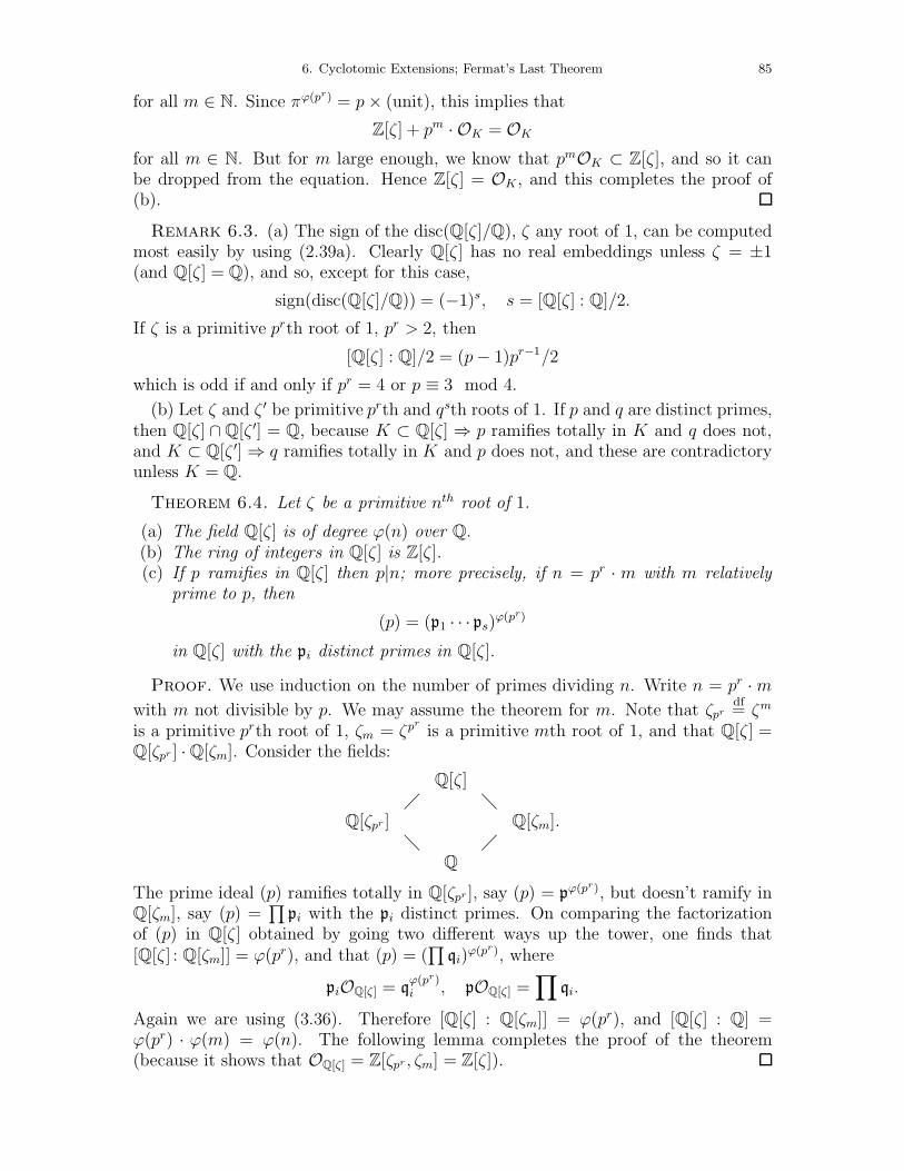
6. Cyclotomic Extensions; Fermat’s Last Theorem 85
for all m ∈ N. Since πϕ(pr) = p× (unit), this implies that
Z[ζ] + pm · OK = OKfor all m ∈ N. But for m large enough, we know that pmOK ⊂ Z[ζ], and so it canbe dropped from the equation. Hence Z[ζ] = OK , and this completes the proof of(b).
Remark 6.3. (a) The sign of the disc(Q[ζ]/Q), ζ any root of 1, can be computedmost easily by using (2.39a). Clearly Q[ζ] has no real embeddings unless ζ = ±1(and Q[ζ] = Q), and so, except for this case,
sign(disc(Q[ζ]/Q)) = (−1)s, s = [Q[ζ] : Q]/2.
If ζ is a primitive prth root of 1, pr > 2, then
[Q[ζ] : Q]/2 = (p− 1)pr−1/2
which is odd if and only if pr = 4 or p ≡ 3 mod 4.
(b) Let ζ and ζ ′ be primitive prth and qsth roots of 1. If p and q are distinct primes,then Q[ζ] ∩Q[ζ ′] = Q, because K ⊂ Q[ζ] ⇒ p ramifies totally in K and q does not,and K ⊂ Q[ζ ′]⇒ q ramifies totally in K and p does not, and these are contradictoryunless K = Q.
Theorem 6.4. Let ζ be a primitive nth root of 1.
(a) The field Q[ζ] is of degree ϕ(n) over Q.(b) The ring of integers in Q[ζ] is Z[ζ].(c) If p ramifies in Q[ζ] then p|n; more precisely, if n = pr · m with m relatively
prime to p, then
(p) = (p1 · · · ps)ϕ(pr)
in Q[ζ] with the pi distinct primes in Q[ζ].
Proof. We use induction on the number of primes dividing n. Write n = pr ·mwith m not divisible by p. We may assume the theorem for m. Note that ζpr
df= ζm
is a primitive prth root of 1, ζm = ζpris a primitive mth root of 1, and that Q[ζ] =
Q[ζpr ] ·Q[ζm]. Consider the fields:
Q[ζ]
Q[ζpr ] Q[ζm].
Q
The prime ideal (p) ramifies totally in Q[ζpr ], say (p) = pϕ(pr), but doesn’t ramify in
Q[ζm], say (p) =∏
pi with the pi distinct primes. On comparing the factorizationof (p) in Q[ζ] obtained by going two different ways up the tower, one finds that[Q[ζ] : Q[ζm]] = ϕ(pr), and that (p) = (
∏qi)
ϕ(pr), where
piOQ[ζ] = qϕ(pr)i , pOQ[ζ] =
∏qi.
Again we are using (3.36). Therefore [Q[ζ] : Q[ζm]] = ϕ(pr), and [Q[ζ] : Q] =ϕ(pr) · ϕ(m) = ϕ(n). The following lemma completes the proof of the theorem(because it shows that OQ[ζ] = Z[ζpr , ζm] = Z[ζ]).
86 6. Cyclotomic Extensions; Fermat’s Last Theorem
Lemma 6.5. Let K and L be finite extensions of Q such that
[KL : Q] = [K : Q] · [L : Q],
and let d = gcd(disc(OK/Z), disc(OL/Z)). Then
OK·L ⊂ d−1OK · OL.Proof. Let α1, ..., αm and β1, ..., βm be integral bases forK and L respectively.
Then αiβj is a basis for K · L over Q. Thus every γ ∈ OK·L can be written uniquelyin the form
γ =∑ij
aijrαiβj, aij, r ∈ Z.
After dividing out any common factors from top and bottom, no prime factor of rwill divide all the aij, and we then have to show that r|d.
Identify L with a subfield of C, and let σ be an embedding of K into C. Then σextends uniquely to an embedding of K · L into C fixing the elements of L (to seethis, write K = Q[α]; then K · L = L[α], and the hypothesis on the degrees impliesthat the minimum polynomial of α doesn’t change when we pass from Q to L; thereis therefore a unique L-homomorphism L[α] → C sending α to σα). On applying σto the above equation, we obtain an equation
σ(γ) =∑ij
aijrσ(αi)βj.
Write xi =∑
j(aij/r)βj, and let σ1, σ2, ..., σm be the distinct embeddings of K intoC. We obtain a system of m linear equations∑
i
σk(αi)xi = σk(γ), k = 1, 2, ..., m,
and Cramer’s rule tells us that
Dxi = Di
where D = det(σj(αi)) and Di ∈ OK·L. According to (2.25), D2 = ∆df= disc(OK/Z),
and so
∆ · xi = DDi ∈ OK·L.But ∆xi =
∑ ∆aij
rβj, and the βjs form an integral basis for OL, and so
∆aij
r∈ Z.
Hence r|∆aij all i, j, and, because of our assumption on r and the aijs, this impliesthat r|∆.
Similarly, r| disc(OL/Z), and so r divides the greatest common divisor ofdisc(OK/Z) and disc(OL/Z).
Remark 6.6. (a) Statement (c) of the theorem shows that if p|n then p ramifiesunless ϕ(pr) = 1. Since ϕ(pr) = pr−1(p − 1), this can only happen if pr = 2. Thusp|n ⇒ p ramifies in Q[ζn] except when p = 2 and n = 2 · (odd number). Note thatQ[ζn] = Q[ζ2n] if n is odd.
(b) In the situation of the lemma,
disc(KL/Q) = disc(K/Q)[L : Q] · disc(L/Q)[K : Q],
6. Cyclotomic Extensions; Fermat’s Last Theorem 87
provided the discriminants on the right are relatively prime. The example Q[i,√5] =
Q[i] · Q[√−5] shows that the condition is necessary, because the extensions have
discriminants 4252, 4, and 20 respectively. Using this, one can show that, for ζn aprimitive nth root of 1,
disc(Q[ζn]/Q) = (−1)ϕ(n)/2nϕ(n)/∏p|n
pϕ(n)/(p−1).
Class numbers of cyclotomic fields. Let ζ be a primitive pth root of 1, p an oddprime. It is known that the class number of Q[ζ] grows quite rapidly with p, and thatin fact the class number is 1 if and only if p ≤ 19.
Here is how to prove that Q[ζ] has class number > 1 when p = 23. The Galoisgroup of Q[ζ] over Q is cyclic of order 22, and therefore has a unique subgroup ofindex 2. Hence Q[ζ] contains a unique quadratic extension K of Q. Since 23 is theonly prime ramifying in Q[ζ], it must also be the only prime ramifying in K, and thisimplies that K = Q[
√−23]. One checks that (2) splits in Q[√−23], say (2) = pq,
that p is not principal, and that p3 is principal. Let P be a prime ideal of Z[ζ]lying over p. Then NP = pf , where f is the residue class degree. Since f divides[Q[ζ] : Q[
√−23]] = 11, we see that f = 1 or 11 (in fact, f = 11). In either case,pf is not principal, and this implies that P is not principal, because the norm of aprincipal ideal is principal.
Because of the connection to Fermat’s last theorem, primes p such that p does notdivide the class number of Q[ζ] are of particular interest. They are called regular.Kummer found a simple test for when a prime is regular: define the Bernoulli numbersBn by the formula
t
et − 1=∞∑n=0
Bntn
n!, Bn ∈ Q;
then p is regular if and only if p divides the numerator of some Bk with k =2, 4, . . . , p − 3. It has long between known that (unfortunately) there are infinitelymany irregular primes, and it still not proved that there are infinitely many regu-lar primes (although the first case of Fermat’s theorem is known for infinitely manyprimes). It is expected that 61% of primes are regular and 39% are irregular.
Units in cyclotomic fields. Let ζ be a primitive nth root of 1, n > 2. Define
Q[ζ]+ = Q[ζ + ζ−1].
For example, if ζ = e2πi/n, then Q[ζ]+ = Q[cos 2πn]. Under any embedding of Q[ζ]
into C, ζ−1 maps to the complex conjugate of ζ, and therefore the image of Q[ζ]+
is fixed under complex conjugation and hence lies in R. Thus Q[ζ]+ has ϕ(n)/2 realembeddings (and no nonreal embeddings), whereas Q[ζ] has ϕ(n) nonreal complexembeddings. Therefore the unit theorem (5.1) shows that the groups of units in Q[ζ]and Q[ζ]+ have the same rank, and so, if u is a unit in Q[ζ], then um ∈ Q[ζ]+ forsome m. In fact a more precise result is known.
Proposition 6.7. Assume n is a prime power; then every unit u ∈ Q[ζ] can bewritten
u = ζ · v
88 6. Cyclotomic Extensions; Fermat’s Last Theorem
with ζ a root of unity and v a unit in Q[ζ]+.
Proof. This is not difficult — see Frohlich and Taylor 1991, VI.1.19, or Washing-ton 1982.
Fermat’s last theorem. Fermat’s last theorem is known to be true for p a regularprime. Here we prove a weaker result, known as the first case of Fermat’s last theorem.
Theorem 6.8. Let p be an odd prime. If the class number of Q[ζ] is not divisibleby p, then there is no integer solution (x, y, z) to
Xp + Y p = Zp
with p xyz.
Let (x, y, z) be a solution of Fermat’s equation with p xyz. After removing anycommon factor, we may suppose that gcd(x, y, z) = 1.
We first treat the case p = 3. The only cubes modulo 9 are −1, 0, 1, and so
x3 + y3 ≡ −2, 0, 2 mod 9, z3 ≡ −1, 1 mod 9,
which are contradictory. Similarly we may eliminate the case p = 5 by looking modulo25. Henceforth we assume p > 5.
If x ≡ y ≡ −z mod p, then −2zp ≡ zp and p|3z, contradicting our hypotheses.Hence one of the congruences can’t hold, and after rewriting the equation xp+(−z)p =(−y)p if necessary, we may assume that p x− y.
The roots of Xp + 1 are −1,−ζ, . . . ,−ζp−1, and so
Xp + 1 =
p−1∏i=0
(X + ζ i).
Hence
p−1∏i=0
(x+ ζ iy) = zp.
The idea of the proof is to exploit this factorization and what we know of the arith-metic of Q[ζ] to obtain a contradiction.
Let p be the unique prime ideal of Z[ζ] dividing (p); thus (see 6.2) p = (1− ζ i) forany i, 1 ≤ i ≤ p− 1.
Lemma 6.9. The elements x+ ζ iy of Z[ζ] are relatively prime in pairs.
Proof. We have to show that there does not exist a prime ideal q dividing x+ ζ iyand x + ζjy for i = j. Suppose there does. Then q|((ζ i − ζj)y) = py, and q|((ζj −ζ i)x) = px. By assumption, x and y are relatively prime, and therefore q = p. Thusx+y ≡ x+ ζ iy ≡ 0 mod p. Hence x+y ∈ p∩Z = (p). But zp = xp+yp ≡ x+y ≡ 0mod p, and so p|z, which contradicts our hypotheses.
Lemma 6.10. For any α ∈ Z[ζ], αp ∈ Z + pZ[ζ].
6. Cyclotomic Extensions; Fermat’s Last Theorem 89
Proof. Write
α = a0 + a1ζ + · · ·+ ap−2ζp−2, ai ∈ Z.
Then
αp ≡ ap0 + ap1 + · · ·+ app−1 mod p,
which lies in Z.
Lemma 6.11. Suppose α = a0 + a1ζ + · · ·+ ap−1ζp−1 with ai ∈ Z and at least oneai = 0. If α is divisible by an integer n, i.e., if α ∈ nZ[ζ], then each ai is divisible byn.
Proof. Since 1 + ζ + · · · + ζp−1 = 0, any subset of 1, ζ, . . . , ζp−1 with p − 1elements will be a Z-basis for Z[ζ]. The result is now obvious.
We can now complete the proof of Theorem 6.8. Consider the equation
p−1∏i=0
(x+ ζ iy) = (z)p
as an equality of ideals in Z[ζ]. Since the factors on the left are relatively prime inpairs, each one must be the pth power of an ideal, say
(x+ ζ iy) = api
for some ideal ai in Z[ζ]. This equation says ai has order dividing p in the class group,but we are assuming that the class group of Z[ζ] is of order prime to p, and so aiitself is principal, say ai = (αi).
Take i = 1, and omit subscripts. Then we have that x+ ζy = uαp for some unit uin Z[ζ]. We apply (6.7) to write u = ζrv where v = v. According to (6.10), there isan a ∈ Z such that αp ≡ a mod p. Therefore
x+ ζy = ζrvαp ≡ ζrva mod p.
Also
x+ ζy = ζ−rvαp ≡ ζ−rva mod p.
On combining these statements, we find that
ζ−r(x+ ζy) ≡ ζr(x+ ζ−1y) mod p,
or
x+ ζy − ζ2rx− ζ2r−1y ≡ 0 mod p. (*)
If 1, ζ, ζ2r−1, ζ2r are distinct, then, because p ≥ 5, Lemma 6.11 implies that p divides xand y, which is contrary to our original assumption. The only remaining possibilitiesare:
(a) 1 = ζ2r; but then (*) says
ζy − ζ−1y ≡ 0 mod p,
and Lemma 6.11 implies p|y, which contradicts our original assumption.
90 6. Cyclotomic Extensions; Fermat’s Last Theorem
(b) 1 = ζ2r−1; then ζ = ζ2r, and (*) says
(x− y)− (x− y)ζ ≡ 0 mod p,
and Lemma 6.11 implies that p|x − y, which contradicts the choice of x and ymade at the start of the proof.
(c) ζ = ζ2r−1; but then (*) says
x− ζ2x ≡ 0 mod p,
and Lemma 6.11 implies that p|x, which contradicts our original assumption.
This completes the proof.
7. Valuations; Local Fields. 91
7. Valuations; Local Fields
In this section, we define the notion of a valuation and study the completions ofnumber fields with respect to valuations.
Valuations. A (multiplicative) valuation on a field K is a function x → |x| : K → Rsuch that
(a) |x| > 0 except that |0| = 0;(b) |xy| = |x||y|(c) |x+ y| ≤ |x|+ |y| (triangle inequality).
If the stronger condition
(c′) |x+ y| ≤ max|x|, |y|holds, then | | is called a nonarchimedean valuation.
Note that (a) and (b) imply that | | is a homomorphism K× → R>0 (multiplicativegroup of positive real numbers). Since R>0 is torsion-free, | | maps all roots of unityin K× to 1. In particular, | − 1| = 1, and | − x| = |x| for all x.
Example 7.1. (a) For any number field K, and embedding σ : K → C, we get avaluation on K by putting |a| = |σa|.
(b) Let ord : K× → Z be an (additive) discrete valuation, and let e be a real numberwith e > 1; then
|a| = (1/e)ord(a), a = 0, |0| = 0
is a nonarchimedean valuation on K. For example, for any prime number p, we havethe p-adic valuation | |p on Q :
|a|p = (1/e)ordp(a).
Usually we normalize this by taking e = p; thus
|a|p = (1/p)ordp(a) = 1/pr if a = a0 · pr with ordp(a0) = 0.
Similarly, for any prime ideal p in a number field K, we have a normalized p-adicvaluation
|a|p = (1/Np)ordp(a).
(c) On any field we can define the trivial valuation: |a| = 1 for all a = 0. When Kis finite, there is no other (because all nonzero elements of a finite field are roots of1).
Nonarchimedean valuations. Recall that this means that, instead of the triangleinequality, we have
|x+ y| ≤ max|x|, |y|.By induction, this condition implies that
|∑
xi| ≤ max|xi|. (*)
Proposition 7.2. A valuation | | is nonarchimedean if and only if it takes boundedvalues on m1 | m ∈ Z.
92 7. Valuations; Local Fields.
Proof. If | | is nonarchimedean, then, for m > 0,
|m1| = |1 + 1 + · · · + 1| ≤ |1| = 1.
As we noted above, | − 1| = |1|, and so | −m1| = |m1| ≤ 1.
Conversely, suppose |m1| ≤ N for all m. Then
|x+ y|n = |∑(
nr
)xryn−r | ≤
∑r
|(
nr
)| |x|r|y|n−r.
Clearly |x|r|y|n−r ≤ max|x|n, |y|n = max|x|, |y|n and
(nr
)is an integer, and so
|x+ y|n ≤ N(n + 1)max|x|, |y|n.On taking nth roots we find that
|x+ y| ≤ N1/n(n+ 1)1/nmax|x|, |y|.When we let n→∞, the terms involving n tend to 1 (to see this, take logs).
Corollary 7.3. If char K = 0, then K has only nonarchimedean valuations.
Proof. In this case, the set m · 1 | m ∈ Z is finite.Aside 7.4. The classical archimedean axiom states that if a and b are nonzero
elements of K, then there is an n ∈ N such that |b| < |na|. The proposition showsthat the nonarchimedean valuations are precisely those for which the archimedeanaxiom fails, whence the name.
As we noted above, a discrete (additive) valuation ord on K determines a valuationby
|x| = e−ord(x),
any e > 1. Taking logs gives loge |x| = −ord(x), or ord(x) = − loge |x|. This suggestshow we might pass from multiplicative valuations to additive valuations.
Proposition 7.5. Let | | be a nontrivial nonarchimedean valuation, and putv(x) = − log |x|, x = 0 (log to base e for any real e > 1). Then v : K× → Rsatisfies the following conditions:
(a) v(xy) = v(x) + v(y);(b) v(x+ y) ≥ minv(x), v(y).If v(K×) is a discrete in R, then it is a multiple of a discrete valuation ord : K×
Z ⊂ R.
Proof. That v satisfies (a) and (b) is obvious. For the last statement, note thatv(K×) is a subgroup of R (under addition). If it is a discrete subgroup, then it is a
lattice (by 4.14), which means that v(K×) = Zc for some c. Now orddf= c−1 · v is an
additive discrete valuation K× Z.
We shall say | | is discrete when |K×| is a discrete subgroup of R>0. Note that,even when |K×| is discrete in R, |K| usually won’t be, because 0 will be a limit pointfor the set |K×|. For example, |pn|p = p−n, which converges to 0 as n→∞.
7. Valuations; Local Fields. 93
Proposition 7.6. Let | | be a nonarchimedean valuation. Then
Adf= a ∈ K | |a| ≤ 1 is a subring of K, with
Udf= a ∈ K | |a| = 1 as its group of units, and
mdf= a ∈ K | |a| < 1 as its unique maximal ideal.
The valuation | | is discrete if and only if m is principal, in which case A is a discretevaluation ring.
Proof. The first assertion is obvious. If | | is discrete, then A and m are the pairassociated (as in 3.28) with the additive valuation − log | |, and so A is a discretevaluation ring and m is generated by any element π ∈ K× such that |π| is the largestelement of |K×| less than one. Conversely, if m = (π), then |K×| is the subgroup ofR>0 generated by |π|.
Remark 7.7. There do exist nondiscrete nonarchimedean valuations. For exam-ple, let Qal be an algebraic closure of Q. We shall see later that the p-adic valuation| |p : Q→ R extends to Qal (in many different ways). Since Qal contains an elementp1/n for all n, we see that |Qal×| * (p−1)1/n = 1/ n
√p for all n, and 1/ n
√p → 1 as
n → ∞. In fact, one can show that |Qal×| = pr | r ∈ Q, which is not discrete inR>0.
Equivalent valuations. Note that a valuation | | defines a metric on K, with dis-tance function
d(a, b) = |a− b|,and hence a topology on K. In more detail, for a ∈ K, the sets
U(a, ε) = x ∈ K | |x− a| < ε, ε > 0,
form a fundamental system of open neighbourhoods of a. A set is open if and only ifit is a union of sets of the form U(a, ε).
For example, for the topology on Q defined by | |p, a and b are close if theirdifference is divisible by a high power of p. In particular, the sequence
1, p, p2, . . . , pn, . . .
converges to 0.
The topology defined by the p-adic valuation | |p is called the p-adic topology onK.
Proposition 7.8. Let | |1, | |2 be valuations on K, with | |1 nontrivial. Thefollowing conditions are equivalent:
(a) | |1, | |2 define the same topology on K;(b) |α|1 < 1⇒ |α|2 < 1;(c) | |2 = | |a1 for some a > 0.
Proof. (a) ⇒ (b): Since |αn| = |α|n, clearly αn → 0 if and only if |α| < 1.Therefore (a) implies that
|α|1 < 1 ⇐⇒ |α|2 < 1.
94 7. Valuations; Local Fields.
(b) ⇒ (c): Because | |1 is nontrivial, there exists a y ∈ K such that |y| > 1. Let
a = log |y|2/ log |y|1,so that
log |y|2 = a · log |y|1,or
|y|2 = |y|a1.Now let x be any nonzero element of K. There is a real number b such that
|x|1 = |y|b1.To prove (c), it suffices to prove that
|x|2 = |y|b2,because then
|x|2 = |y|b2 = |y|ab1 = |x|a1.
Let m/n, n > 0, be a rational number > b. Then
|x|1 = |y|b1 < |y|mn1
and so
|xn/ym|1 < 1.
From our assumption (b), this implies that
|xn/ym|2 < 1
and so
|x|2 < |y|mn2 .
This is true for all rational numbers mn> b, and so
|x|2 ≤ |y|b2.A similar argument with rational numbers m
n< b shows that
|x|2 ≥ |y|b2,and so we have equality, which completes the proof of (a).
Two valuations are said to be equivalent if they satisfy the conditions of the propo-sition.
7. Valuations; Local Fields. 95
Properties of discrete valuations. We make some easy, but important, observa-tions about discrete valuations.
(7.9.1) For an additive valuation, we are given that
ord(a+ b) ≥ minord(a), ord(b)and we checked (3.27 et seq.) that this implies that equality holds if ord(a) = ord(b).For multiplicative valuations, we are given that
|a+ b| ≤ max|a|, |b|,and a similar argument shows that equality holds if |a| = |b|. This has the followingconsequences.
(7.9.2) Recall that we define a metric on K by setting d(a, b) = |a− b|. I claim thatif x is closer to b than it is to a, then d(a, x) = d(a, b). For we are given that
|x− b| < |x− a|,and this implies that
|b− a| = |b− x+ x− a| = |x− a|.(7.9.3) Suppose
a1 + a2 + · · ·+ an = 0.
Then an argument as in the subsection on Eisenstein extensions (end §3) shows thatthe maximum value of the summands must be attained for at least two values of thesubscript.
Complete list of valuations for Q. We now give a complete list of the valuationson Q (up to equivalence). We write | |∞ for the valuation on Q defined by the usualabsolute value on R, and we say that | |∞ is normalized.
Theorem 7.10 (Ostrowski). Let | | be a nontrivial valuation on Q.
(a) If | | is archimedean, then | | is equivalent to | |∞.(b) If | | is nonarchimedean, then it is equivalent to | |p for exactly one prime p.
Proof. Let m,n be integers > 1. Then we can write
m = a0 + a1n + · · ·+ arnr
with the ai integers, 0 ≤ ai < n, nr ≤ m. Let N = max1, |n|. By the triangleinequality,
|m| ≤∑|ai||n|i ≤
∑|ai|N r.
We know
r ≤ log(m)/ log(n),
(log relative to some e > 1) and the triangle inequality shows that
|ai| ≤ |1 + · · ·+ 1| = ai|1| = ai ≤ n.
On putting these into the first inequality, we find that
|m| ≤ (1 + r)nN r ≤ (1 +logm
logn)nN
log mlog n .
96 7. Valuations; Local Fields.
In this inequality, replace m with mt (t an integer), and take tth roots:
|m| ≤(1 +
t logm
log n
)1t
n1tN
log mlog n .
Now let t→∞. The terms involving t tend to 1, and so
|m| ≤ Nlog mlog n . (*)
Case (i): For all integers n > 1, |n| > 1.
In this case N = |n|, and (*) yields:
|m|1/ logm ≤ |n|1/ logn.By symmetry, we must have equality, and so there is an c > 1 such that
c = |m|1/ logm = |n|1/ logn
for all integers m,n > 1. Hence
|n| = clogn = elog c logn = nlog c, all integers n > 1.
Let a = log c, and rewrite this
|n| = |n|a∞, all integers n > 1,
where | |∞ is the usual absolute value on Q. Since both | | and | |a∞ are homomorphismsQ× → R>0, the fact that they agree on a set of generators for the group Q× (theprimes and −1) implies that they agree on all of Q×.
Case (ii): For some n > 1, |n| ≤ 1.
In this case, N = 1, and (*) implies |m| ≤ 1 for all integers m. Therefore thevaluation is nonarchimedean. Let A be the associated local ring and m its maximalideal. From the definition of A, we know that Z ⊂ A. Then m∩Z is a prime ideal inZ (because m is a prime ideal), and it is nonzero for otherwise the valuation wouldbe trivial. Hence m∩Z = (p) for some p. This implies that |m| = 1 if m is an integernot divisible by p, and so |npr| = |p|r if n is a rational number whose numerator anddenominator are not divisible by p. If a is such that |p| = (1/p)a; then |x| = |x|ap forall x ∈ Q.
Theorem 7.11 (Product Formula). For p = 2, 3, 5, 7, ...,∞, let | |p be the corre-sponding normalized valuation on Q. For any nonzero rational number a∏
|a|p = 1 (product over all p including ∞).
Proof. Let α = a/b, a, b ∈ Z. Then |α|p = 1 unless p|a or p|b. Therefore |α|v = 1for all but finite many v’s, and so the product is really finite.
Let π(a) =∏ |a|v. Then π is a homomorphism Q× → R×, and so it suffices to
show that π(−1) = 1 and π(p) = 1 for each prime number p. The first is obvious,because | − 1| = 1 for all valuations | |. For the second, note that
|p|p = 1/p, |p|q = 1, q a prime = p, |p|∞ = p.
The product of these numbers is 1.
7. Valuations; Local Fields. 97
The primes of a number field. LetK be an algebraic number field. An equivalenceclass of valuations on K is called a prime of K.
Theorem 7.12. Let K be an algebraic number field. There exists exactly oneprime of K
(a) for each prime ideal p;(b) for each real embedding;(c) for each conjugate pair of complex embeddings.
Proof. See §8.In each equivalence class of valuations of K we select a normalized valuation13 as
follows:
for a prime ideal p of OK , |a|p = (1/Np)ordp(a) = (Op : (a))−1;for a real embedding σ : K → R, |a| = |σa|;for a nonreal complex embedding σ : K → C, |a| = |σa|2.
Note that this last is not actually a valuation, because it doesn’t satisfy the trianglelaw. There are various ways of getting around this problem the best of which is simplyto ignore it.
Notations. We generally write v for a prime. If it corresponds to a prime ideal p ofOK , then we call it a finite prime, and we write pv for the ideal. If it correspondsto a (real or nonreal) embedding of K, then we call it an infinite (real or complex)prime. We write | |v for a valuation in the equivalence class. If L ⊃ K and w and vare primes of L and K such that | |w restricted to K is equivalent to | |v, then we saythat w divides v, or w lies over v, and we write w|v. For a finite prime, this meansPw ∩ OK = pv or, equivalently, that Pw divides pv · OL. For an infinite prime, itmeans that w corresponds to an embedding σ : L → C that extends the embeddingcorresponding to v (or its complex conjugate).
Theorem 7.13 (Product Formula). For each prime v, let | |v be the normalizedvaluation. For any nonzero α ∈ K,∏
|α|v = 1 (product over all primes of K).
Proof. The product formula for a general number field follows from the productformula for Q and the next result.
Lemma 7.14. Let L be a finite extension of a number field K.
(a) Each prime on K extends to a finite number of primes of L.(b) For any prime v of K and α ∈ L×,∏
w|v|α|w = |NmL/K α|v.
13These are the most natural definitions for which the product formula hold. Alternatively, letKv be the completion of K with respect to the valuation v, and let µ be a Haar measure on (Kv,+)— it is uniquely determined up to a nonzero constant. For any nonzero a ∈ Kv, µa(U) df= µ (aU) isalso a Haar measure on (Kv,+), and so µa = c(a)µ for some constant c(a). In fact, c(a) = |a|, thenormalized valuation of a.
98 7. Valuations; Local Fields.
Proof. See §8.Remark 7.15. The product formula is true in two other important situations.
(a) Let K be a finite extension of k(T ) where k is a finite field. According to(7.3), the valuations of K are all discrete, and hence correspond to discrete valuationrings in K. As in the number field case, we can normalize a valuation by setting|a|v = (1/Nv)ordv(a) where Nv is the number of elements in the residue field of thediscrete valuation ring and ordv : K
× Z. Then∏
v |a|v = 1. The proof of this iseasy when K = k(T ), and the general case is obtained by means of a result like (7.14).
(b) Let K be a finite extension of k(T ) where k is an algebraically closed field. Inthis case we only look at primes that are trivial when restricted to k. All such primesare nonarchimedean, and hence correspond to discrete valuations ordv : K
× Z. Fixan e > 1, and define |a|v = (1/e)ordv(a) for every v. Then
∏ |a|v = 1 for all a ∈ K×.This of course is equivalent to the statement
∑ordv(a) = 0.
For example, let X be a compact Riemann surface, and let K be the field of mero-morphic functions on X. For each point P of X we have a discrete valuation, definedby ordP (f) = m or −m according as f has a zero or pole of order m at P . The valu-ations ordP are precisely the valuations on K trivial on C ⊂ K, and so the productformula for K is simply the statement that f has as many zeros as poles.
The proof of this runs as follows: the Cauchy integral formula implies that if f isa nonconstant meromorphic function on an open set U in C, and Γ is the orientedboundary of a compact set C contained in U , then∫
Γ
f ′(z)f(z)
dz = 2πi(Z − P )
where Z is the number of zeros of f in C and P is the number of poles of f , bothcounted with multiplicities. This formula also holds for compact subsets of manifolds.If the manifoldM is itself compact, then we can take C = M , which has no boundary,and so the formula becomes
Z − P = 0,
i.e., ∑ordP (f) = 0, P ∈M.
Completions. Let K be a field with a nontrivial valuation. A sequence (an) ofelements in K is called a Cauchy sequence if, for every ε > 0, there is an N such that
|an − am| < ε, all m,n > N.
The field K is said to be complete if every Cauchy sequence has a limit in K. (Thelimit is necessarily unique.)
Example 7.16. Consider the sequence in Z
4, 34, 334, 3334, . . . .
7. Valuations; Local Fields. 99
As
|am − an|5 = 5−n (m > n),
this is a Cauchy sequence for the 5-adic topology on Q. Note that
3 · 4 = 12, 3 · 34 = 102, 3 · 334 = 1002, 3 · 3334 = 10002, . . .
and so 3 · an − 2→ 0 as n→∞. Thus limn→∞ an = 2/3 ∈ Q.
There is a similar notion of Cauchy series. For example, any series of the form
a−np−n + · · ·+ a0 + a1p+ · · · + ampm + · · · , 0 ≤ ai < p,
is a Cauchy series in Q for the p-adic topology.
Theorem 7.17. Let K be a field with a valuation | |. Then there exists a complete
valued field (K, | |) and a homomorphism K → K preserving the valuation that isuniversal in the following sense: any homomorphism K → L from K into a completevalued field (L, | |) preserving the valuation, extends uniquely to a homomorphism
K → L. The image of K in K is dense.
Proof. (Sketch) The uniqueness of (K, | |) is obvious from the universal property.
Let K be the closure of K in K. Then K is complete, and so the homomorphismK → K extends to K — this implies that K = K, and so K is dense in K.
We now construct K. Every point of K will be the limit of a sequence of pointsin K, and the sequence will be Cauchy. Two Cauchy sequences will converge to thesame point in K if and only if they are equivalent in the sense that
limn→∞|an − bn| = 0.
This suggests defining K to be the set of equivalence classes of Cauchy sequences inK. Define addition and multiplication of Cauchy sequences in the obvious way, andverify that K is a field. There is a canonical map K → K sending a to the constantCauchy sequence a, a, a, . . . , which we use to identify K with a subfield of K . Wecan extend a homomorphism from K into a second complete valued field L to K bymapping the limit of a Cauchy sequence in K to its limit in L.
For a prime v of K, we write Kv for the completion of K with respect to v. Whenv corresponds to a prime ideal p, we write Kp for the completion, and Op for the ringof integers in Kp. For example, Qp is the completion of Q with respect to the p-adic
valuation | |p. We write Zp (not Zp) for the ring of integers in Qp (the ring of p-adicintegers).
Completions in the nonarchimedean case. Let | | be a discrete nonarchimedeanvaluation on K, and let π be an element of K with largest value < 1 (therefore πgenerates the maximal ideal m in the valuation ring A). Such a π is called a localuniformizing parameter.
The set of values is
|K| = cm | m ∈ Z ∪ 0, c = |π|.
100 7. Valuations; Local Fields.
Let a ∈ K×, and let an be a sequence in K converging to a. Then |an| → |a| (because| | is a continuous map), and so |a| is a limit point for the set |K×|. But |K×| isclosed (being discrete), and so |a| ∈ |K×|. Thus |K| = |K|, and so | | is a discrete
valuation on K also. Let ord : K× Z be a normalized discrete additive valuationcorresponding to | |; then ord extends to a normalized discrete valuation on K.
Note that if an → a = 0, then |an| → |a| = 0, and (because |K×| is discrete),|an| = |a| for all n large enough.
The ring associated with | | in K is
A = a ∈ K | |a| ≤ 1.Clearly A is the set of limits of Cauchy sequences in A, and it is therefore the closureof A in K. The maximal ideal in A is
m = a ∈ K | |a| < 1.Again it is the set of limits of Cauchy sequences in m, and so it is the closure of m.Similarly, mn is the closure of mn. Let π be an element with ord(π) = 1; then π
generates m in A and m in A.
Lemma 7.18. For any n, the map A/mn → A/mn is an isomorphism.
Proof. Note that
mn = a ∈ A | |a| ≤ |π|n = a ∈ A | |a| < |π|n−1is both open and closed in A. Because it is closed, the map is injective; because mn
is open, the map is surjective.
Proposition 7.19. Choose a set S of representatives for A/m, and let π generatem. The series
a−nπ−n + · · · + a0 + a1π + · · ·+ amπm + · · · , ai ∈ S
is a Cauchy series, and every Cauchy series is equivalent to exactly one of this form.Thus each element of K has a unique representative of this form.
Proof. Let sM =∑M
i=−n aiπi. Then
|sM − sN | ≤ |π|M+1, if M < N,
which shows that the sequence sM is Cauchy. Let α ∈ K. Because |K| = |K|, we canwrite α = πnα0 with α0 a unit in A. From the definition of S, we see that there existsan a0 ∈ S such that α0− a0 ∈ m. Now α0−a0
π∈ A, and so there exists an a1 ∈ S such
that α0−a0
π− a1 ∈ m. Now there exists an a2 such that α0−a0−a1π
π2 − a2 ∈ m, etc. Inthe limit,
α0 = a0 + a1π + · · · , α = πnα0.
Note that
|∑ aiπi| = |πm|
if am is the first nonzero coefficient. Therefore∑
aiπi = 0 (if and) only if ai = 0 for
all i. This proves the uniqueness.
7. Valuations; Local Fields. 101
Thus, for example, every equivalence class of Cauchy sequences in Q for | |p has aunique representative of the form
a−np−n + · · ·+ a0 + a1p+ a2p2 + · · · , 0 ≤ ai < p.
Note that the partial sums of such a series are rational numbers. It is as easy to workwith such series as with decimal expansions of real numbers — just remember highpowers of p are small, and hence the first to be ignored.
We explain this in more detail. The maps
Z/(pn)→ Z(p)/(pn)→ Zp/(p
n)
are both bijective (see 3.11 for the first map). Let α ∈ Zp. Because the map isbijective, for all n, there is an an ∈ Z such that α ≡ an mod pn. Note that, if n < m,an ≡ am mod pn, which implies that (an) is a Cauchy sequence. Let
an ≡ c0 + c1p+ · · ·+ cn−1pn−1 mod pn, 0 ≤ ci ≤ p− 1;
then
α =∑i≥0
cipi.
Conversely, if α =∑
cipi, 0 ≤ ci ≤ p − 1, then c0, c1, . . . is the unique sequence of
integers, 0 ≤ ci ≤ p− 1, such that
α ≡n−1∑i=0
cipi mod pn.
If α ∈ Qp but not Zp, then pmα ∈ Zp for a sufficiently large m, and the abovearguments can be applied to it.
Example 7.20. To illustrate how to work with p-adic numbers, I prove that −1is a square in Q5. We have to find a series
a0 + a15 + a252 + · · · , ai = 0, 1, 2, 3, or 4
such that
(a0 + a15 + a252 + ...)2 + 1 = 0.
We first need that
a20 + 1 ≡ 0 mod 5.
Thus we must take a0 = 2 or 3; we choose 2 (choosing 3 would lead to the other root).Next we need
(2 + a15)2 + 1 ≡ 0 mod 52,
and so we want
5 + 20a1 ≡ 0 (mod 52).
We must take a1 = 1. Suppose we have found
cn = a0 + a15 + a252 + · · ·+ an5
n
such that
c2n + 1 ≡ 0 (mod 5n+1),
102 7. Valuations; Local Fields.
and consider cn + an+15n+1. We want
(cn + an+15n+1)2 + 1 ≡ 0 (mod 5n+2),
for which we need that
c2n + 1 + 2cnan+15n+1 ≡ 0 (mod 5n+2),
or that
2cnan+15n+1 ≡ (−1− c2n) (mod 5n+2),
or that
2cnan+1 ≡ (−1− c2n)/5n+1 (mod 5),
or that
4an+1 = (−1− c2n)/5n+1 (mod 5).
Since 4 is invertible modulo 5, we can always achieve this. Hence we obtain a seriesconverging to −1.
There is a leisurely, and very detailed, discussion of Qp in the first chapter of N.Koblitz, p-adic Numbers, p-adic Analysis, and Zeta-Functions, Springer, 1977.
Aside 7.21. Those who have taken a course in commutative algebra will knowanother method of completing a local ring R, namely
R′ = lim←
R/mn = (an) | an ∈ R/mn, an+1 ≡ an mod mn.In the case that R is a discrete valuation ring, this definition agrees with the above.There is an injective homomorphism
R→ R′, a → (an), an = a mod πn.
We can define a homomorphism R′ → R as follows: let (an) ∈ R′, and choose arepresentative a′n for an in R; then (a′n) is an Cauchy sequence whose equivalenceclass is independent of the choices of the a′n, and we can map (an) to (a′n). It is easyto see that the map R′ → R is surjective, and it follows that it is an isomorphism.
Newton’s lemma. The argument in the above example works much more generally.Let f(X) = X2+1. Then all we in fact used was that f(X) has a simple root modulo5.
In the rest of this subsection, A is a complete discrete valuation ring and π generatesits maximal ideal (unless we say otherwise).
Proposition 7.22. Let f(X) ∈ A[X], and let a0 be a simple root of f(X) mod π.Then there is a unique root a of f(X) with a ≡ a0 mod π.
Proof. Suppose we have found an ≡ a0 mod π such that
f(an) ≡ 0 mod πn+1.
Let an+1 = an + hπn+1, h ∈ A. We want
f(an + hπn+1) ≡ 0 mod πn+2.
Recall (trivial Taylor’s expansion) that, for any polynomial f,
f(c+ t) = f(c) + t · f ′(c) + · · ·
7. Valuations; Local Fields. 103
where f ′(X) is the formal derivative of f(X). Then
f(an + hπn+1) = f(an) + hπn+1 · f ′(an) + · · · ,which we want ≡ 0 mod πn+2. Hence we must take h so that
h = −f(an)πn+1
· f ′(an)−1 mod π.
This is possible because πn|f(an) andf ′(an) ≡ f ′(a0) mod π,
which is nonzero, and hence invertible, mod π.
There is a stronger form of the proposition. Recall Newton’s approximation methodfor finding a solution to f(x) = 0, where f is a function of a real variable. Startingfrom an a0 such that f(a0) is small, define a sequence a1, a2, ... by putting
an+1 = an − f(an)/f′(an).
Often an converges to a root of f(x). In the above proof, this is what we did, but thesame argument can be made to work more generally.
Theorem 7.23 (Newton’s lemma). Let f(X) ∈ A[X]. Let a0 ∈ A satisfy
|f(a0)| < |f ′(a0)|2.Then there is a unique root a of f(X) such that
|a− a0| ≤∣∣∣∣ f(a0)
f ′(a0)2
∣∣∣∣ .Proof. Define a sequence a0, a1, . . . by setting
an+1 = an − f(an)
f ′(an)
and prove that it is a Cauchy sequence converging to a root of f(X). See, for example,EC 2.8. [In fact, it is not necessary to assume that | | is discrete — see Lang 1970, p.42.]
Proposition 7.22 shows that a simple factor of degree 1 of f(X) mod π lifts to afactor of f(X). This generalizes.
Theorem 7.24 (Hensel’s lemma). Let k be the residue field of A; for f(X) ∈A[X], write f(X) for the image of f in k[X]. Consider a monic polynomial f(X) ∈A[X]. If f(X) factors as f = g0h0 with g0 and h0 monic and relatively prime (ink[X]), then f itself factors as f = gh with g and h monic and such that g = g0 andh = h0. Moreover, g and h are uniquely determined, and (g, h) = A[X].
We first prove that (g, h) = A[X] (such a pair is said to be strictly coprime; in k[X]strictly coprime just means coprime, i.e., relatively prime).
Lemma 7.25. Let A be a local ring with residue field k. If f, g ∈ A[X] are suchthat f and g are relatively prime and f is monic, then (f, g) = A[X].
Proof. Let M = A[X]/(f, g). As f is monic, this is a finitely generated A-module. As (f , g) = k[X], we have that (f, g) + mA[X] = A[X] and so mM = M .Now Nakayama’s Lemma (1.3) implies that M = 0.
104 7. Valuations; Local Fields.
We next prove uniqueness of g and h.
Lemma 7.26. Let A be a local ring with residue field k. Suppose f = gh = g′h′
with g, h, g′, h′ all monic, and g = g′, h = h′ with g and h relatively prime. Theng = g′ and h = h′.
Proof. From the preceding lemma we know that (g, h′) = A[X], and so thereexist r, s ∈ A[X] such that gr + h′s = 1. Now
g′ = g′gr + g′h′s = g′gr + ghs,
and so g divides g′. As both are monic and have the same degree, they must beequal.
Finally, we prove the existence of g and h. We are given that there exist monicpolynomials g0, h0 ∈ A[X] such that
f − g0h0 ∈ π · A[X].
Suppose we have constructed monic polynomials gn, hn such that
f − gnhn ≡ 0 mod πn+1A[X]
and gn ≡ g0, hn ≡ h0 mod πA[X]. We want to find u, v ∈ A[X] such that
f − (gn + πn+1u)(hn + πn+1v) ≡ 0 mod πn+2A[X],
i.e., we want
(f − gnhn)− πn+1(uhn + gnv) ≡ 0 mod πn+2A[X].
Thus we are looking for polynomials u, v in A[X] such that
uhn + gnv ≡ (f − gnhn)/πn+1 mod πA[X].
From (7.25), we know that hn and gn are strictly coprime, and so we can always findsuch polynomials u, v.
Remark 7.27. By induction, the theorem shows that a factorization of f into aproduct of relatively prime polynomials in k[X] lifts to a factorization in A[X]. Forexample, in Fp[X], Xp−X splits into p distinct factors, and so it also splits in Zp[X].Hence Zp contains the p − 1st roots of 1. More generally, if K has a residue field kwith q elements, then K contains q roots of the polynomial Xq − X. Let S be theset of these roots. Then
a → a : S → k,
is a bijection preserving multiplication (but not, of course, addition) – the elementsof S are called the Teichmuller representatives for the elements of the residue field.
Remark 7.28. Theorems 7.23 and 7.24 are both stronger versions of 7.22. Thereis in fact a stronger version of 7.23. For a polynomial h =
∑ciX
i, define
‖h‖ = max |ci|.Let
f(X) = anXn + an−1Xn−1 + · · ·+ a0 ∈ A[X]
7. Valuations; Local Fields. 105
have |an| = 1 (i.e., an is a unit). Let g0(X) and h0(X) be polynomials in A[X] withdegrees r and s respectively, and suppose that
‖f(X) − g0(X)h0(X)‖ < |Res(g0(X), h0(X))|2
where Res denotes the resultant. Then f(X) factors in A[X] as the product of apolynomial of degree r and a polynomial of degree s. The proof follows the samegeneral lines as the above proofs. In fact, the hypothesis can be replaced by
‖f(X) − g0(X)h0(X)‖ < |disc(f)|.(For this, see Cassels 1986, p107.)
Note that, this gives an algorithm for factoring polynomials in Qp[X] (for example).Given f(X), compute disc(f). If this is zero, then f and f ′ have a common factor(which we can find by the Euclidean algorithm). Otherwise ord(disc(f)) = m for somem, and it is enough to consider factorizations of f into polynomials with coefficientsin the finite ring Z/pmZ. Apparently the fastest algorithms for factoring polynomialsin Z[X] begin by factoring in Zp[X] for an appropriate prime p — computers seemto have no problem handling polynomials of degree 200. (But Problems 10, no. 3,shows that there are irreducible polynomials in Z[X] of arbitrarily large degree thatfactor in all the rings Zp[X] into polynomials of low degree.)
Extensions of nonarchimedean valuations. We explain how to extend a valua-tion to a larger field.
Theorem 7.29. Let K be complete with respect to a discrete valuation | |K, andlet L be a finite separable extension of K of degree n. Then | | extends uniquely toa discrete valuation | |L on L, and L is complete for the extended valuation. For allβ ∈ L,
|β|L = |NmL/K β|1/nK .
Proof. Let A be the discrete valuation ring in K, and let B be its integral closurein L. Let p be the maximal ideal of A. We know from (3.30) that B is a Dedekinddomain, and the valuations of L extending | |p correspond to the ideals of B lyingover p.
Suppose that there are distinct prime ideals P1 and P2 in B dividing p. Therewill be a β ∈ B such that P1 ∩ A[β] = P2 ∩ A[β]; for example, choose β ∈ Bsuch that β ∈ P1, β /∈ P2. Let f(X) be the minimum polynomial of β over K, sothat A[β] ∼= A[X]/(f(X)). Because f(X) is irreducible in A[X] and A is complete,Hensel’s lemma shows that f (X) (image of f(X) in k[X], k = A/p) must be a powerof an irreducible polynomial. Then
A[β]/pA[β]≈ k[X]/(f(X))
is a local ring, which contradicts the fact that A[β] has two prime ideals containingp.
Hence | |p extends uniquely to a valuation | | on L.
Clearly, | |p also extends uniquely to the Galois closure L′ of L. For each σ ∈Gal(L/K), consider the map L → C, β → |σβ|. This is again a valuation of L, and
106 7. Valuations; Local Fields.
so the uniqueness implies that |β| = |σβ|. Now
|Nm(β)| = |∏
σβ| = |β|n
which implies the formula.
Finally, we have to show that L is complete. Let e1, . . . , en be a basis for B as anA-module, and let (α(m)) be a Cauchy sequence in L. Write α(m) = a1(m)e1+ · · ·+an(m)en, with ai(m) ∈ K. For each i, ai(m) is a Cauchy sequence, and if ai denotes
its limit, then αdf= a1e1 + · · ·+ anen is the limit of the sequence α(m).
Remark 7.30. It is obvious from the criterion (7.2) that a nonarchimedean valu-ation can only extend to a nonarchimedean valuation. It is possible to prove (7.29)without assuming that the valuation | | on K is discrete or even nonarchimedean, butthe proof is then completely different, and much longer — we shall in fact need this
in the §8, and so I should have included it. The formula |β|L = |NmL/K β|1/nK showsthat | |L is discrete if and only if | |K is discrete.
Corollary 7.31. Let K be as in the theorem, and let Ω be a (possibly infinite)algebraic extension of Q. Then | | extends in a unique way to a valuation | | on Ω.
Proof. The theorem shows that | | extends in a unique way to any finite subex-tension of Ω, and hence it extends uniquely to Ω.
Remark 7.32. In the last corollary, the extended valuation is still nonar-chimedean, but it need not be discrete, and Ω need not be complete. However,the completion of Ω is again algebraically closed.
For example as we noted in (7.7), the valuation on the algebraic closure Qalp of Qp is
not discrete, and Problems 10, no. 4, shows that Qalp is not complete. The completion
of Qalp is often denoted Cp because it plays the same role for the p-adic valuation on
Q that C plays for the real valuation. (In fact Cp ≈ C as abstract fields becausethey are both algebraically closed, and they both have a transcendence basis withcardinality equal to that of R. The isomorphism is as far from being canonical as itis possible to get — its construction requires the axiom of choice.)
Corollary 7.33. Let K and L be as in the theorem; then n = ef where n = [L :K], e is the ramification index, and f is the degree of the residue field extension.
Proof. We know from (3.36) that n =∑
eifi. In this case, there is only oneprime dividing p and so the formula becomes n = ef.
When e = n, so that pB = pn, we say that L is totally ramified over K; whenf = n, we say that L is unramified over K.
Note that the valuation ring B of L is the integral closure of the valuation ring Aof K.
Many of the results proved above for complete discrete valuation rings hold alsofor Henselian local rings (see §4 of my notes on Etale Cohomology).
Remark 7.34. Let K be complete with respect to a discrete valuation, and let Lbe a finite extension of K. Let P and p be the maximal ideals in the rings of integersA and B of K and L. Then pB = Pe where e is the ramification index. Let π and
7. Valuations; Local Fields. 107
Π be generators of p and P. The normalized valuations ordK and ordL on K and Lare characterized by equations:
ordK(π) = 1, ordL(Π) = 1.
Note that π = Πe × unit, and so
ordK = e−1ordL.
If we denote the extension of ordK to L by ord, then
ord(L×) = e−1Z.
This characterizes the ramification index.
Newton’s polygon. Let K be complete with respect to a discrete valuation. Let ordbe the corresponding additive valuation ord : K× Z, and extend ord to a valuationord : Kal× → Q. For a polynomial
f(X) = Xn + a1Xn−1 + · · · + an, ai ∈ K,
define the Newton polygon14 of f(X) to be the lower convex hull of the set of points
Pidf= (i, ord(ai)), i = 0, ..., n.
In more detail, rotate the negative y-axis counter-clockwise about P0 = (0, 0) until ithits a Pi — the first segment of the Newton polygon is the line P0Pi1 where Pi1 is thepoint furthest from P0 on the rotated y-axis. Repeat the process rotating about Pi1,etc.. The resulting polygon starts at P0 and ends at Pn; each of its segments beginsand ends at a Pi; each Pi either lies on the polygon or is above it; any line joining twopoints of the polygon has no point that is below the polygon (this is what we meanby the Newton polygon being lower convex).
Proposition 7.35. Suppose that the Newton polygon of f(X) ∈ K[X] has seg-ments of x-length ni and slope si. Then f(X) has exactly ni roots α (in Kal) with
ord(α) = si.
Moreover, the polynomial fi(X)df= Πord(αi)=si
(X − αi) has coefficients in K.
Proof. In proving the first part, we don’t have to assume that f(X) has coeffi-cients in K—any finite extension of K will do. Thus it suffices to prove the followingstatement: let f(X) =
∏(X − αj); if exactly ni of the αj ’s have ordsi, then the
Newton polygon of f(X) has a segment of slope si and x-length ni.
We prove this by induction on n = deg(f). If n = 1, then it is obvious. Assume itfor n, and put
g(X) = (X − α)f(X) = Xn+1 + b1Xn + b2X
n−1 + · · ·+ bn+1.
Note that bi = ai − αai−1.Case (i). ord(α) < s1. Recall ord(a + b) ≥ minord(a), ord(b), with equality if
ord(a) = ord(b). Using this, one finds that
14Most people write the polynomial a0 + a1X + · · · + Xn when they define Newton polygons.This is slightly less convenient than the way I do it, but allows you to define the Newton polygon ofa power series.
108 7. Valuations; Local Fields.
the Newton polygon of g is obtained from that of f by adding a segment of slopeord(α) and x-length 1, and moving the Newton polygon of f to start at (1, ord(α)).This is what the proposition predicts.
Case (ii). ord(α) = s1. In this case, the initial segment of slope s1 is lengthenedby 1, and the rest of the polygon is as before. This is what the proposition predicts.
The remaining cases are similar.
We now prove the second statement. Let α be a root of f(X), and let mα(X) bethe minimum polynomial of α. As we saw in the proof of (7.29), ord(α′) = ord(α) forall conjugates α′ of α, i.e., for all roots of mα(X). Because f(α) = 0, mα(X)|f(X),and the remark just made implies that in fact mα(X)|fi(X) where si = ord(α).If β is a root of fi(X)/mα(X), then a similar argument shows that mβ(X)|(fi/mα).Continuing in this way, we find that fi(X) is a product of polynomials with coefficientsin K.
Example 7.36. Consider the polynomial
f(X)df= X3 +X2 + 2X − 8.
By testing ±1, ±2, ±4, ±8 (actually, by asking Maple) one sees that this polynomialis irreducible over Q. The Newton polygon of f relative to ord2 has slopes 0, 1, 2,each with x-length 1. Therefore f splits in Q2[X], and it has roots α1, α2, α3 withords 0, 1, 2.
Locally compact fields. We now look at the compactness properties of our fields.
Proposition 7.37. Let K be complete with respect to a nonarchimedean discretevaluation. Let A be the ring of integers in K and let m be the maximal ideal in A.Then A is compact if and only if A/m is finite.
Proof. Let S be a set of representatives for A/m. We have to show that A iscompact if and only if S is finite.
⇒: Clearly m = x ∈ K | |x| < 1 is open in K. As A is the disjoint union of theopen sets s+ m, s ∈ S, S must be finite if A is compact.
⇐: Recall that a metric space X is compact if and only if it is complete and totallybounded (this means that for any r > 0, there is a finite covering of X by open ballsof radius r). But every element of A can be written
s0 + s1π + s2π2 + · · ·+ snπ
n + · · · , si ∈ S.
For a fixed n, there are only finitely many sums
s0 + s1π + s2π2 + · · · + snπ
n, si ∈ S,
and every element of A is within |πn+1| of such an element.
Corollary 7.38. Assume that the residue field is finite. Then pn, 1 + pn, andA× are all compact.
Proof. They are all closed subsets of A.
Definition 7.39. A local field is a field K with a nontrivial valuation | | (as de-fined at the start of this section) such thatK is locally compact (and hence complete).
7. Valuations; Local Fields. 109
Remark 7.40. It is possible to give a complete classification of local fields.
(a) Let K be a field that is complete with respect to an archimedean valuation| |; then K is isomorphic to R of C, and the valuation is equivalent to the usualabsolute value (Theorem of Ostrowski, see Janusz 1996, II.4). Thus for archimedeanvaluations, completeness implies local compactness.
(b) A nonarchimedean local field K of characteristic zero is isomorphic to a finiteextension of Qp, and the valuation is equivalent to the (unique) extension of the p-adicvaluation. (To prove this, note that, by assumption, K contains Q. The restrictionof | | to Q can’t be the trivial valuation, because otherwise A× wouldn’t be compact.Therefore (see 7.10) | | induces a valuation on Q equivalent to the p-adic valuationfor some prime number p. The closure of Q in K is therefore Qp. If K has infinitedegree over Qp, it will not be locally compact.)
(c) A nonarchimedean local field K of characteristic p = 0 is isomorphic to the fieldof formal Laurent series k((T )) over a finite field k. The field k((T )) is the completionof k(T ) for the valuation defined by the ideal (T ) ⊂ k[T ]; it consists of finite-tailedformal power series:
∞∑i≥−n
aiTi.
Unramified extensions of a local field. Again K is a field complete with respectto a discrete valuation | |. To avoid problems with separability, we assume that Kand the residue field k are both perfect15—of course in the case we are particularlyinterested in, K has characteristic zero and k is finite. Let A be the discrete valuationring in K corresponding to | |.
If L is an algebraic (possibly infinite) extension of K, we can still define
B = α ∈ L | |α| ≤ 1
p = α ∈ B | |α| < 1and call B/p the residue field of L.
Proposition 7.41. Let L be an algebraic extension of K, and let l be the residuefield of L. The map K ′ → k′ sending an unramified extension K ′ of K contained inL to its residue field k′ is a one-to-one correspondence between the sets
K ′ ⊂ L, finite and unramified over K ↔ k′ ⊂ l, finite over k.Moreover:
(a) if K ′ ↔ k′ and K ′′ ↔ k′′, then K ′ ⊂ K ′′ ⇐⇒ k′ ⊂ k′′;(b) if K ′ ↔ k′, then K ′ is Galois over K if and only if k′ is Galois over k, in which
case there is a canonical isomorphism
Gal(K ′/K)→ Gal(k′/k).
15When k is not perfect, we should define L/K to be unramified if (a) the ramification index is1, and (b) the residue field extension is separable. These conditions imply that L/K is separable.With this definition, (7.41) continues to hold without K and k being assumed to be perfect
110 7. Valuations; Local Fields.
Proof. Let k′ be a finite extension of k. We can write it k′ = k[a]. Let f0(X) bethe minimum polynomial of a over k, and let f(X) be any lifting of f0(X) to A[X].As a is a simple root of f0(X), Newton’s lemma (7.22) shows that there is a (unique)α ∈ L such that f(α) = 0 and α ≡ a mod p. Now K ′ =df K[α] has residue field k′.Thus K ′ → k′ is surjective. Suppose that K ′ and K ′′ are unramified extensions of Kin L with the same residue field k′. Then K ′ · K ′′ is an unramified extension of K(see 6.5 and 6.6b) with residue field k′. Hence
[K ′ ·K ′′ : K] = [k′ : k] = [K ′ : K],
and so K ′′ = K ′.Statement (a) is obvious.
Assume K ′ is Galois over K; then Gal(K ′/K) preserves A′ (the valuation ring inK ′) and its maximal ideal, and so we get a map Gal(K ′/K) → Aut(k′/k). Writek′ = k[a], and let g(X) ∈ A[X] be such that g(X) ∈ k[X] is the minimum polynomialof a. Let α ∈ A′ be the unique root of g(X) such that α = a. Because K ′ is Galoisover K, g(X) splits in A′[X], and this implies that g(X) splits in k′[X], and so k′ isGalois over k. Let f = [k′ : k] = [K ′ : K], and let α1, . . . , αf be the roots of g(X).Then
α1, ..., αf = σα | σ ∈ Gal(L/K).Because g(X) is separable, the αi are distinct modulo p, and this shows that theimage of the map Gal(K ′/K)→ Gal(k′/k) has order f , and hence is an isomorphism.Conversely, suppose k′/k is Galois. Again write k′ = k[a], and α ∈ A′ lift a. Itfollows from Hensel’s lemma that A′ contains the conjugates of α, and hence that K ′
is Galois over K.
Corollary 7.42. There is a field K0 ⊂ L containing all unramified extensionsof K in L (called the largest unramified extension of K in L). In fact, it is obtainedfrom K by adjoining all roots of 1 of order prime to the characteristic of k.
Proof. This is an obvious consequence of the theorem.
Corollary 7.43. The residue field of Kal is kal; there is a subfield Kun of Kal
such that a subfield L of Kal, finite over K, is unramified if and only if L ⊂ Kun.(Recall that we are assuming k and K to be perfect.)
Proof. Let f0(X) be any polynomial in k[X], and let f(X) be any lift of f0(X)to A[X]. Then Kal contains all the roots of f(X), and so the residue field k′ of Kal
contains all the roots of f0(X). Hence k′ is algebraic over k, and every polynomial ink[X] splits in k′, and so it must be the algebraic closure of k.
Remark 7.44. For those familiar with the language of category theory, we can bea little more precise: there is an equivalence between the category of finite unramifiedextensions of K and the category of finite (separable) extensions of k.
Example 7.45. Let K be a local field of characteristic zero (hence a finite exten-sion of Qp for some p), and let q be the order of the residue field k of K.
Recall from (FT §4.6) that, for each n, there is an extension kn of k of degree n,and that kn is unique up to k-isomorphism; it is the splitting field of Xqn −X. The
7. Valuations; Local Fields. 111
Galois group Gal(kn/k) is a cyclic group of order n, having as canonical generatorthe Frobenius element x → xq.
Therefore, for each n, there is an unramified extension Kn of K of degree n, and itis unique up to K-isomorphism; it is the splitting field of Xqn −X; the Galois groupGal(Kn/K) is a cyclic group of order n, having as canonical generator the Frobeniuselement σ which is determined by the property
σβ ≡ βq (mod p),
all β ∈ B. (Here B is the discrete valuation ring in Kn, and p is the nonzero primeideal in B.)
Totally ramified extensions of K. Let K be a complete discretely-valued nonar-chimedean field, and let π be a local uniformizing parameter for K. A polynomialf(X) ∈ K[X] is said to be Eisenstein if it is Eisenstein for the maximal ideal of thering of integers in K, i.e., if
f(X) = a0Xn + a1X
n−1 + · · ·+ an, with |a0| = 1, |ai| < 1, |an| = |π|.Equivalently,
ord(a0) = 0, ord(ai) > 0, ord(an) = 1,
for the normalized additive valuation. Equivalently, the Newton polygon of f(X) hasonly one segment, which has slope 1
n, n = deg f . Eisenstein polynomials allow us to
give an explicit description of all totally ramified extensions of K.
Proposition 7.46. Let L be a finite extension of K. Then L/K is totally ramifiedif and only if L = K[α] with α a root of an Eisenstein polynomial.
Proof. ⇐: Suppose L = K[α] with α a root of an Eisenstein polynomial f(X)of degree n. If ord is the extension of the normalized discrete (additive) valuation onK to L, then ord(α) = 1/n. This implies that the ramification index of L/K is ≥ n.But it can’t be greater than n, and so it is exactly n — L is totally ramified over K.(Compare the proof of 6.2.)
⇒: Suppose L is a totally ramified extension of K of degree n. Let α be a generatorof the maximal ideal in the ring of integers in L; thus ord(α) = 1/n if ord extends thenormalized discrete valuation on K. The elements 1, α, ..., αn−1 represent differentcosets of ord(K×) in ord(L×), and so it is impossible to have a nontrivial relation
a0 + a1α + · · ·+ an−1αn−1 = 0, ai ∈ K
(because of 7.9.3). Hence L = K[α]. The elements 1, α, . . . , αn−1, αn are linearlydependent over K, and so we have a relation:
αn + a1αn−1 + · · ·+ an = 0, ai ∈ K.
Applying (7.9.3) again, we see that the minimum ord of a summand must be attainedfor two terms. The only way this can happen is if ord(ai) > 0 for all i and ord(an) =ord(αn) = 1, i.e., if
∑aiX
i is an Eisenstein polynomial.
Remark 7.47. Let L be a finite totally ramified extension of K. Let A and B bethe discrete valuation rings in K and L, and let π and Π be a prime elements in A
112 7. Valuations; Local Fields.
and B. I claim that B = A[Π]. The argument is the same as in the proof of 6.2 (seealso Problems 8, no. 1). Because B and A have the same residue field,
A[Π] + ΠB = B.
The discriminant of 1,Π,Π2, . . . is a unit×πm for some m, and so
pcB ⊂ A[Π] ⊂ B
for some c. As before, these two conditions suffice to imply that B = A[Π].
Ramification groups. Let L be a finite Galois extension of K, and assume that
the residue field k of K is perfect. As we have noted, Gdf= Gal(L/K) preserves the
valuation on L. In particular, it preserves
B = α ∈ L | |α| ≤ 1, p = α ∈ L | |α| < 1.Let Π be a prime element of L (so that p = (Π)). We define a sequence of subgroupsG ⊃ G0 ⊃ G1 ⊃ · · · by the condition:
σ ∈ Gi ⇐⇒ |σα− α| < |Π|i, all α ∈ B.
The group G0 is called the inertia group, the group G1 is called the ramification group,and the groups Gi, i > 1, are called the higher ramification groups of L over K.
Lemma 7.48. The Gi are normal subgroups of G, and Gi = 1 for i large enough.
Proof. (a) For σ, τ ∈ G, we have
|τ−1στα− α| = |σ(τα)− (τα)|(because |x| = |τx|). As α runs through B, so also does τα, and so τ−1στ ∈ Gi
exactly when σ does.
(b) If σ = 1, then σα = α for some α ∈ B. Hence σ /∈ Gi as soon as |σα − α| ≥|Π|i.
Theorem 7.49. Let L/K be a Galois extension, and assume that the residue fieldextension l/k is separable.
(a) The fixed field of G0 is the largest unramified extension K0 of K in L, and
G/G0 = Gal(K0/K) = Gal(l/k).
(b) For i ≥ 1, the group
Gi = σ ∈ G0 | |σΠ− Π| < |Π|i.
Proof. (a) Let K0 be the largest unramified extension in L (see 7.42). Then σK0
is also unramified, and so it is contained in K0. Thus K0 is Galois over K, and thecanonical map Gal(K0/K) → Gal(l/k) is an isomorphism (see 7.41). By definitionG0 is the kernel of G→ Gal(l/k), and so K0 is its fixed field.
(b) Let A0 be the discrete valuation ring in K0. Then B = A0[Π] (by 7.45). SinceG0 leavesA0 fixed, in order to check that σ ∈ Gi it suffices to check that |σα−α| < |Π|ifor the element α = Π.
7. Valuations; Local Fields. 113
Corollary 7.50. We have an exhaustive filtration G ⊃ G0 ⊃ · · · such that
G/G0 = Gal(l/k);
G0/G1 → l×;Gi/Gi+1 → l.
Therefore, if k is finite, then Gal(L/K) is solvable.
Proof. Let σ ∈ G0; then σΠ is also a prime element and so σΠ = uΠ with u aunit in B. The map σ → u mod p is a homomorphism G0 → l× with kernel G1.
Let σ ∈ Gi. Then |σΠ − Π| ≤ |Π|i+1, and so σΠ = Π + aΠi+1 some a ∈ B. Themap σ → a (mod p) is a homomorphism Gi → l with kernel Gi+1.
An extension L/K is said to be wildly ramified if p|e where p = char(k). Otherwiseit is said to be tamely ramified. Hence for a Galois extension
L/K is unramified ⇐⇒ G0 = 1,and
L/K is tamely ramified ⇐⇒ G1 = 1.Krasner’s lemma and applications. Again let K be complete with respect toa discrete nonarchimedean valuation | |, and extend the valuation (uniquely) to avaluation on Kal. It is clear from our discussion of unramified extensions of K thatroots of distinct polynomials f(X) and g(X) will often generate the same extensionof K; in fact, this will be true if f = g and both are irreducible in k[X]. Krasner’slemma and its consequences show that the roots of two polynomials will generate thesame extension if they are sufficiently close.
Proposition 7.51 (Krasner’s lemma). . Let α, β ∈ Kal, and assume that α isseparable over K[β]. If α is closer to β than to any conjugate of α (over K), thenK[α] ⊂ K[β].
Proof. Let σ be an embedding of K[α, β] into Kal fixing K[β]. By Galois theory,it suffices to show that σα = α. But
|σα− β| = |σα− σβ| = |α− β|because σβ = β and |σ ∗ | = | ∗ |. Hence
|σα− α| = |σα− β + β − α| ≤ |α− β|.Since σα is a conjugate of α over K, the hypothesis now implies that σα = α.
Now assume K has characteristic zero (to avoid complications). As before, forh(X) =
∑ciX
i, we define ‖h‖ = max|ci|. Note that if h(X) varies in a familyof monic polynomials for which ‖h‖ remains bounded, then the maximum value of aroot of h is bounded; in fact, if ∑
ciβi = 0,
we must have |βn| ≤ |cjβj| for some j < n, and so |β|n−j ≤ |cj|.Fix a monic irreducible polynomial f(X) in K[X], and let
f(X) =∏
(X − αi), αi ∈ Kal.
114 7. Valuations; Local Fields.
The αi must be distinct. Let g(X) be a second monic polynomial in K[X], andsuppose that ‖f − g‖ is small. For any root β of g(X), |f(β)| = |(f − g)(β)| is small(because ‖f − g‖ small implies that ‖g‖ is bounded, and hence |β| is bounded). But
|f(β)| =∏|β − αi|.
In order for this to be small, at least one term |β − αi| must be small. By taking‖f − g‖ small enough, we can force β to be closer to one root αi than αi is to anyother αj . That is, we can achieve:
|β − αi| < |αi − αj|, all j = i.
In this case, we say that β belongs to αi. Krasner’s lemma then says that K[αi] ⊂K[β], and because f and g have the same degree, they must be equal. We haveproved:
Proposition 7.52. Let f(X) be a monic irreducible polynomial of K[X], and letα be a root of f . Then any monic polynomial g(X) ∈ K[X] sufficiently close to f(X)is also irreducible, and it has a root β that belongs to α. For such a root K[α] = K[β].
Corollary 7.53. Let K be a finite extension of Qp. Then there is a finite exten-sion L of Q contained in K such that [L : Q] = [K : Qp] and L ·Qp = K.
Proof. Write K = Qp[α], and let f(X) be the minimum polynomial of α overQp. Choose g(X) ∈ Q[X] sufficiently close to f(X), and let L = Q[β] for β a root ofg(X) belonging to α.
Now consider two monic polynomials f and g, and write αi for the roots of f andβi for the roots of g. For ‖f − g‖ sufficiently small, every root of g will belong to aroot of f , and I claim that they will belong to distinct roots, i.e., the roots can benumbered so that βi belongs to αi. For each choice s of n elements from α1, ..., αn(possibly with repetitions), we form the polynomial fs(X) =
∏αi∈s(X − αi). If two
roots of g(X) belong to the same root of f(X), then g(X) will be close to fs(X) forsome fs = f . But if we choose g to be closer to f than f is to any fs, this will beimpossible. We have proved:
Proposition 7.54. Assume K is of characteristic zero. If two monic irreduciblepolynomials f and g are sufficiently close, then each root of g will belong to exactlyone root of f , and so
K[α] | α a root of f = K[β] | β a root of g.Proposition 7.55. Assume K has characteristic zero and has finite residue field.
Then, up to isomorphism, there are only finitely many totally ramified extensions ofQp of a given degree.
Proof. We fix an n and show that there are only finite many extensions of degree≤ n. Each point of
(a1, ..., an) ∈ p× p× p× · · · × A×π
defines an Eisenstein polynomial of degree n, namely,
f(X) = Xn + a1Xn−1 + · · ·+ an,
115
and hence a finite set of totally ramified extensions of degree n, namely, thosegenerated by the roots of f(X). According to the last proposition, each point ofp × p × p × · · · × A×π has a neighbourhood such that the points in the neighbour-hood all give the same extensions of K. In (7.38) we showed that the factors ofp × p × p × · · · × A×π are compact, hence the product is compact, and so a finitenumber of these neighbourhoods will cover it.
Remark 7.56. We proved above that
(i) every finite extension L of K contains a largest unramified extension of K;
(ii) for each m ≥ 1, there is an unramified extension of degree m of K, and anytwo such extensions are K-isomorphic.
Fix an n; then each extension L ofK of degree n can be realized as a totally ramifiedextension of degree n/m of the (unique) unramified extension of degree m, some mdividing n. Clearly there are only finitely many such L’s (up to K-isomorphism).
A Brief Introduction to PARI. Pari is a program designed for computationsin number theory. It was written by H. Cohen and others, and is availablefrom ftp://megrez.math.u-bordeaux.fr/pub/pari/. See also the Pari home pagehttp://pari.home.ml.org/. It runs under Windows 95 and other operating sys-tems. The following are a few commands for version 2 (they have been changed fromversion 1.x).
To start PARI on a network, type gp To quit PARI, type \qnfbasis(f) finds an integral basis for the field generated by a root of f .
nfdisc(f) finds the discriminant of f .
polcyclo(n) finds the nth cyclotomic polynomial.
polgalois(f) finds the Galois group of f (f irreducible of degree ≤ 11).
newtonpoly(f,p) finds the Newton polygon of f .
factor(f) finds the factors of f .
factormod(f,p) factor f modulo p.
quadunit(x) finds the fundamental unit in the real quadratic field with discrimi-nant x.
The syntax for polynomials is similar to that in Maple, e.g., x^2+3*x+5.
116
8. Global Fields
A global field is defined to be an algebraic number field (finite extension of Q) or afunction field in one variable over a finite field (finite extension of Fq(T ) for some q).We are mainly interested in the number field case.
Extending valuations. LetK be a field with a valuation | | (archimedean or discretenonarchimedean), and letL be a finite separable extension ofK. WhenK is complete,we know that there is a unique extension of | | to L (see 7.29, 7.30), and we want tounderstand the extensions when K is not complete.
Write L = K[α], and let f(X) be the minimum polynomial of α over K. Let | |′be an extension of | | to L. Then we can form the completion L of L with respect to| |′, and obtain a diagram:
L → L| |K → K.
Then L = K[α] (because every element ξ of L is the limit of a Cauchy sequence ξ(n)in L; write ξ(n) =
∑ai(n)α
n, ai(n) ∈ K; then each ai(n) is a Cauchy sequence in
K, with limit ai say in K, and ξ =∑
aiαi). Let g(X) be the minimum polynomial
of α over K. Since f(α) = 0, g(X)|f(X), and so with each extension of | |, we have
associated an irreducible factor of f(X) in K[X].
Conversely, let g(X) be a monic irreducible factor of f(X) in K[X], and let K[x] =
K[X]/(g(X)). Then we obtain a diagram:
Lα →x→ K[x]
| |K → K.
According to (7.29, 7.30), the valuation on K extends uniquely to K[x], and thisinduces a valuation on L extending | |.
These two operations are inverse, and so we have proved the following result:
Proposition 8.1. Let L = K[α] be a finite separable extension of K, and letf(X) be the minimum polynomial of α over K. Then there is a natural one-to-onecorrespondence between the extensions of | | to L and the irreducible factors of f(X)
in K[X].
There is a more canonical way of obtaining the completions of L for the variousextensions of | |.
Proposition 8.2. Let | | be a valuation on K (archimedean or discrete nonar-
chimedean) and let L be a finite separable extension of K. Let K be the completionof K with respect to | |. Then | | has finitely many extensions | |1, . . . , | |g to L; if Lidenotes the completion of L with respect to the valuation | |i, then
L⊗K K ≈ ∏Li.
8. Global Fields 117
Proof. Since L is separable over K, L = K[α] ≈ K[X]/(f(X)) for some element
α ∈ L and its minimum polynomial f(X). Suppose f(X) factors in K[X] as
f(X) = f1(X) · f2(X) · · · fg(X)
with fi(X) monic and irreducible. Then (see 1.13)
L ⊗K K = K[α]⊗K K ≈ K[X]/((f(X)) ≈∏K[X]/(fi(X))
and so the proposition follows from (8.1).
Remark 8.3. Suppose now that K is a number field, that OL = OK [α], and that
| | = | |p for some prime ideal p in OK. Because fi(X) is irreducible in K[X], Hensel’slemma shows that, modulo p, fi(X) is a power of an irreducible polynomial, say,
fi(X) = gi(X)ei .
Then
f(X) =g∏i=1
gi(X)ei ,
and (3.43) tells us that
pOL =∏
Peii , Pi = (p, gi(α)).
The valuations extending | |p correspond to the primes Pi, and so the two descriptionsof the extensions agree.
Corollary 8.4. In the situation of the Proposition, for any element α ∈ L,
NmL/K(α) =∏
NmLi/K(α), TrL/K(α) =
∑TrLi/K
(α).
(in the ith factor or summand on the right, α is regarded as an element of Li).
Proof. By definition the norm and trace of α are the determinant and trace ofthe K-linear map x → αx : L→ L. These don’t change when L is tensored with K,and it easy to see that norms and traces in products break up into products and sumsrespectively.
Example 8.5. According to Maple
f(X) = X6 + 5X5 + 5X3 + 25X + 125
is irreducible in Q[X]. Its Newton polygon for ord5 has three segments of x-lengths3, 2, 1 respectively, and so it has at least three factors in Q5. The discriminant off(X) is
24511(59)(365587),
and so according to (7.28), to find the number of factors of f(X) in Q5[X], it sufficesto factor in modulo 511. Better, according to Pari, version 2, f(X) has exactly 3irreducible factors in Q5[X]. (Type factorpadic(f,p,r) where r is the precisionrequired.)
Suppose we find a factorization
f(X) = f1(X)f2(X)f3(X)
118 8. Global Fields
(to whatever degree of accuracy we wish). To compute |β|i, map β =∑
cjαj to
βi =∑
cjαji ∈ Li
df= Q5[αi], αi a root of fi(X), and use that
|β|i = |βi|i = |NmLi/Q5 β|1/deg fi
i .
The product formula. Before proving the product formula for a number field, weneed one extra fact for local fields.
Let K be a local field with normalized valuation | |. Recall that this means that | |is the usual absolute value if K is R, the square of the usual valuation if K is C, and|a| = (1/Np)ord(a) if the valuation is defined by a prime ideal p.
Let L be a finite separable extension of K, and let | | be the unique extension of| | to L. Let ‖ ‖ be the normalized valuation on L corresponding to | |. What is therelation of ‖ ‖ to | |?
Lemma 8.6. In the above situation, ‖a‖ = |a|n, where n = [L : K].
Proof. When K is archimedean, there are only two cases to consider, and bothare obvious. Thus, assume K is nonarchimedean. Since, by assumption, ‖ ‖ = | |cfor some c, we only have to check that the formula holds for a prime element π of K.Let Π be a prime element of L, and let P = (Π) and p = (π); then π = (unit)× Πe,and so
‖π‖ = ‖Πe‖ = (1/NP)e = (1/Np)ef = |π|n,as required.
Alternatively, use (7.34). For a ∈ K, we have
‖a‖ df= NP−ordLa 7.34
= (Npf )−e·ordKa = |a|ef = |a|n.
Proposition 8.7. Let L/K be a finite extension of number fields. For any primev of K and α ∈ L, ∏
w|v‖α‖w = ‖NmL/K α‖v.
Here ‖ ‖w and ‖ ‖v denote the normalized valuations for the primes w and v.
Proof. Let | |i, i = 1, 2, . . . , g, be the extensions of ‖ ‖v to L, and let ‖ ‖i be thenormalized valuation corresponding to | |i. Then
‖NmL/K α‖v 8.4= ‖∏g
i=1 NmLi/Kα‖v =
∏gi=1 ‖NmLi/K
α‖v7.29=
∏gi=1 |α|n(i)i
8.6=
∏gi=1 ‖α‖w,
where ni = [Li : K].
Theorem 8.8 (Product formula). Let K be an algebraic number field; for allnonzero α ∈ K, ∏
w
‖α‖w = 1,
where the product is over the primes of K and ‖ ‖w is the normalized valuation forthe prime w.
8. Global Fields 119
Proof. We have ∏w
‖α‖w =∏v
(∏w|v‖α‖w) =
∏v
‖Nmα‖v
where v runs through the primes 2, 3, 5, 7, ...,∞ of Q. The last product is 1 by(7.11).
Remark 8.9. E. Artin and Whaples (Bull. Amer. Math. Soc. 51 (1946), 469–492) proved the following characterization of global fields. Let K be a field with a setV of primes (equivalence classes of valuations) satisfying the following axioms.
Axiom I. There is a set of representatives | |v for the primes such that, for anynonzero a ∈ K, |a|v = 1 for only finitely many v and
Πv|a|v = 1 (product over all v ∈ V).
Axiom II. There exists at least one prime v for which Kv is a local field.
Then K is a global field, and V consists of all the primes for K.
Throughout his career, E. Artin promoted the idea that if only one could under-stand the similarities between function fields and number fields sufficiently well, thenone could transfer proofs from function fields to number fields (e.g. the proof of theRiemann hypothesis!). This hasn’t worked as well as he hoped, but the analogy hasstill been very fruitful. In the above paper, he suggested one should develop numbertheory and class field theory as much as possible working only from the axioms.
Decomposition groups. Let L be a finite Galois extension of a number field K,and let G = Gal(L/K). For a valuation w of L, we write σw for the valuation suchthat |σα|σw = |α|w, i.e., |α|σw = |σ−1α|w. For example, if w is the prime defined bya prime ideal P, then σw is the prime defined by the prime ideal σP, because
|α|σw < 1 ⇐⇒ σ−1α ∈ P ⇐⇒ α ∈ σP.
The group G acts on the set of primes of L lying over a fixed prime v of K, and wedefine the decomposition (or splitting) group of w to be the stabilizer of w in G; thus
Gw = σ ∈ G | σw = w.Equivalently, Gw is the set of elements of G that act continuously for the topologydefined by | |w. Each σ ∈ Gw extends uniquely to a continuous automorphism of Lw.Note that Gτw = τGwτ
−1.
Proposition 8.10. The homomorphism Gw → Gal(Lw/Kv) just defined is anisomorphism.
Proof. Clearly the map is injective, and so (Gw : 1) ≤ [Lw : Kv]. The valuationσw has decomposition group σGwσ
−1, which has the same order as Gw, and so wealso have (Gw : 1) ≤ [Lσw : Kv]. The number of distinct w’s dividing v is (G : Gw),and so
(G : 1) = (G : Gw)(Gw : 1) ≤∑
σ∈G/Gw
[Lσw : Kv](8.2)
≤ [L : K].
Hence equality holds: (Gw : 1) = [Lw : Kv] (and G acts transitively on the primesdividing v, which we knew already from the proof of 3.36).
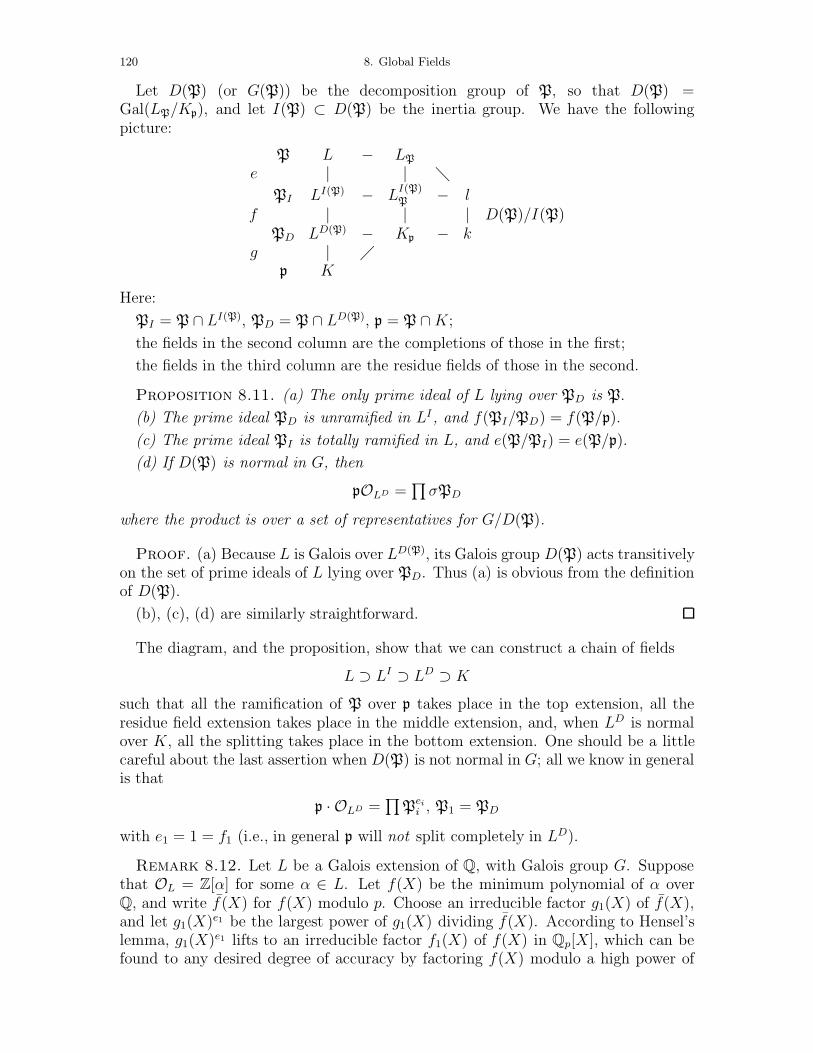
120 8. Global Fields
Let D(P) (or G(P)) be the decomposition group of P, so that D(P) =Gal(LP/Kp), and let I(P) ⊂ D(P) be the inertia group. We have the followingpicture:
P L − LP
e | | PI LI(P) − L
I(P)P
− lf | | | D(P)/I(P)
PD LD(P) − Kp − kg |
p K
Here:
PI = P ∩ LI(P), PD = P ∩ LD(P), p = P ∩K;
the fields in the second column are the completions of those in the first;
the fields in the third column are the residue fields of those in the second.
Proposition 8.11. (a) The only prime ideal of L lying over PD is P.
(b) The prime ideal PD is unramified in LI , and f(PI/PD) = f(P/p).
(c) The prime ideal PI is totally ramified in L, and e(P/PI) = e(P/p).
(d) If D(P) is normal in G, then
pOLD =∏
σPD
where the product is over a set of representatives for G/D(P).
Proof. (a) Because L is Galois over LD(P), its Galois group D(P) acts transitivelyon the set of prime ideals of L lying over PD. Thus (a) is obvious from the definitionof D(P).
(b), (c), (d) are similarly straightforward.
The diagram, and the proposition, show that we can construct a chain of fields
L ⊃ LI ⊃ LD ⊃ K
such that all the ramification of P over p takes place in the top extension, all theresidue field extension takes place in the middle extension, and, when LD is normalover K, all the splitting takes place in the bottom extension. One should be a littlecareful about the last assertion when D(P) is not normal in G; all we know in generalis that
p · OLD =∏
Peii , P1 = PD
with e1 = 1 = f1 (i.e., in general p will not split completely in LD).
Remark 8.12. Let L be a Galois extension of Q, with Galois group G. Supposethat OL = Z[α] for some α ∈ L. Let f(X) be the minimum polynomial of α overQ, and write f (X) for f(X) modulo p. Choose an irreducible factor g1(X) of f(X),and let g1(X)e1 be the largest power of g1(X) dividing f(X). According to Hensel’slemma, g1(X)e1 lifts to an irreducible factor f1(X) of f(X) in Qp[X], which can befound to any desired degree of accuracy by factoring f(X) modulo a high power of
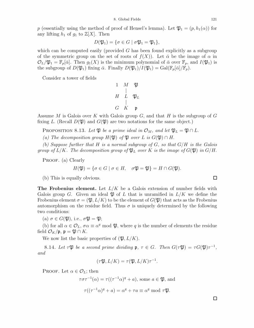
8. Global Fields 121
p (essentially using the method of proof of Hensel’s lemma). Let P1 = (p, h1(α)) forany lifting h1 of g1 to Z[X]. Then
D(P1) = σ ∈ G | σP1 = P1,which can be computed easily (provided G has been found explicitly as a subgroupof the symmetric group on the set of roots of f(X)). Let α be the image of α inOL/P1 = Fp[α]. Then g1(X) is the minimum polynomial of α over Fp, and I(P1) isthe subgroup of D(P1) fixing α. Finally D(P1)/I(P1) = Gal(Fp[α]/Fp).
Consider a tower of fields
1 M P|
H L PL
|G K p
Assume M is Galois over K with Galois group G, and that H is the subgroup of Gfixing L. (Recall D(P) and G(P) are two notations for the same object.)
Proposition 8.13. Let P be a prime ideal in OM , and let PL = P ∩ L.(a) The decomposition group H(P) of P over L is G(P) ∩H.
(b) Suppose further that H is a normal subgroup of G, so that G/H is the Galoisgroup of L/K. The decomposition group of PL over K is the image of G(P) in G/H.
Proof. (a) Clearly
H(P) = σ ∈ G | σ ∈ H, σP = P = H ∩ G(P).
(b) This is equally obvious.
The Frobenius element. Let L/K be a Galois extension of number fields withGalois group G. Given an ideal P of L that is unramified in L/K we define theFrobenius element σ = (P, L/K) to be the element of G(P) that acts as the Frobeniusautomorphism on the residue field. Thus σ is uniquely determined by the followingtwo conditions:
(a) σ ∈ G(P), i.e., σP = P;
(b) for all α ∈ OL, σα ≡ αq mod P, where q is the number of elements the residuefield OK/p, p = P ∩K.
We now list the basic properties of (P, L/K).
8.14. Let τP be a second prime dividing p, τ ∈ G. Then G(τP) = τG(P)τ−1,and
(τP, L/K) = τ (P, L/K)τ−1.
Proof. Let α ∈ OL; thenτστ−1(α) = τ ((τ−1α)q + a), some a ∈ P, and
τ ((τ−1α)q + a) = αq + τa ≡ αq mod τP.
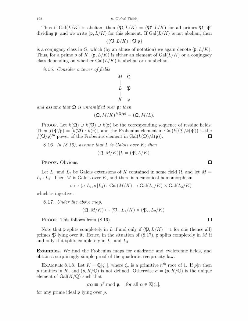
122 8. Global Fields
Thus if Gal(L/K) is abelian, then (P, L/K) = (P′, L/K) for all primes P, P′
dividing p, and we write (p, L/K) for this element. If Gal(L/K) is not abelian, then
(P, L/K) | P|pis a conjugacy class in G, which (by an abuse of notation) we again denote (p, L/K).Thus, for a prime p of K, (p, L/K) is either an element of Gal(L/K) or a conjugacyclass depending on whether Gal(L/K) is abelian or nonabelian.
8.15. Consider a tower of fields
M Q|L P|K p
and assume that Q is unramified over p; then
(Q,M/K)f(P/p) = (Q,M/L).
Proof. Let k(Q) ⊃ k(P) ⊃ k(p) be the corresponding sequence of residue fields.Then f(P/p) = [k(P) : k(p)], and the Frobenius element in Gal(k(Q)/k(P)) is thef(P/p)th power of the Frobenius element in Gal(k(Q)/k(p)).
8.16. In (8.15), assume that L is Galois over K; then
(Q,M/K)|L = (P, L/K).
Proof. Obvious.
Let L1 and L2 be Galois extensions of K contained in some field Ω, and let M =L1 · L2. Then M is Galois over K, and there is a canonical homomorphism
σ → (σ|L1, σ|L2) : Gal(M/K) → Gal(L1/K) ×Gal(L2/K)
which is injective.
8.17. Under the above map,
(Q,M/K) → (P1, L1/K) × (P2, L2/K).
Proof. This follows from (8.16).
Note that p splits completely in L if and only if (P, L/K) = 1 for one (hence all)primes P lying over it. Hence, in the situation of (8.17), p splits completely in M ifand only if it splits completely in L1 and L2.
Examples. We find the Frobenius maps for quadratic and cyclotomic fields, andobtain a surprisingly simple proof of the quadratic reciprocity law.
Example 8.18. Let K = Q[ζn], where ζn is a primitive nth root of 1. If p|n thenp ramifies in K, and (p,K/Q) is not defined. Otherwise σ = (p,K/Q) is the uniqueelement of Gal(K/Q) such that
σα ≡ αp mod p, for all α ∈ Z[ζn],
for any prime ideal p lying over p.
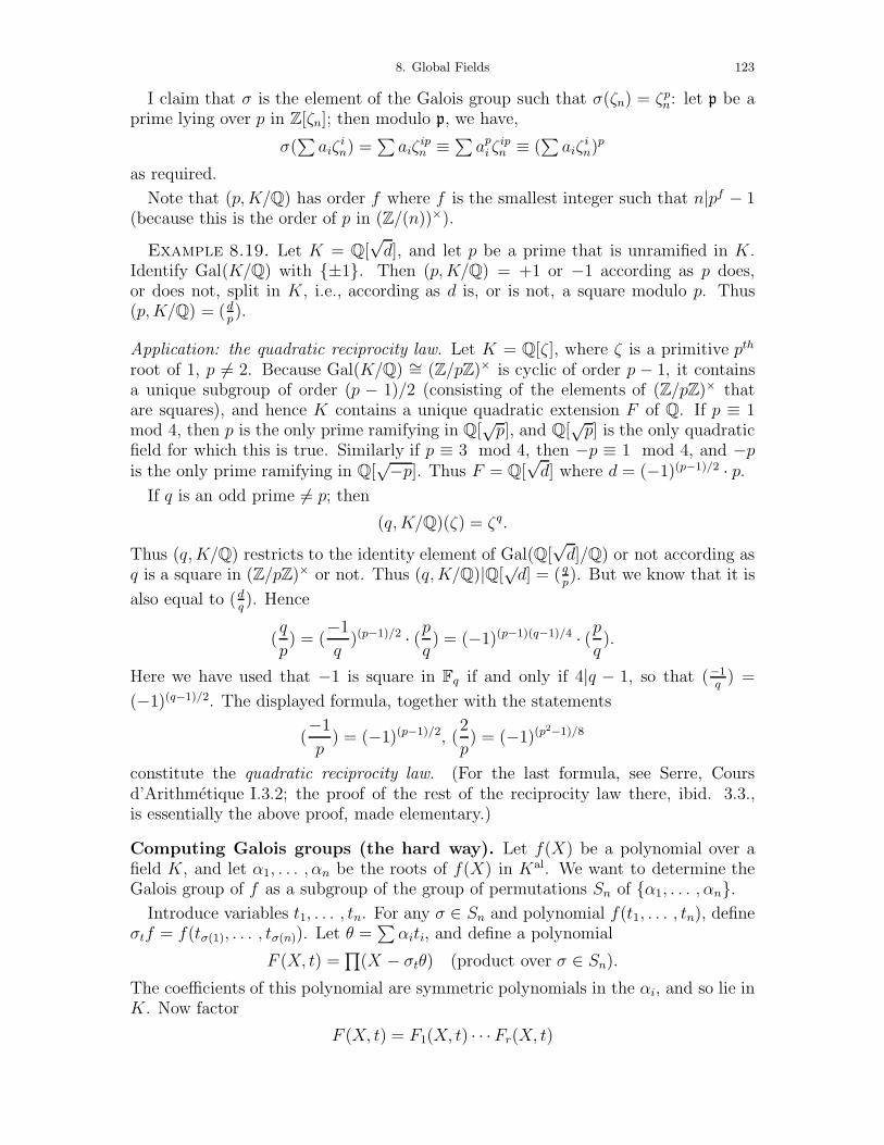
8. Global Fields 123
I claim that σ is the element of the Galois group such that σ(ζn) = ζpn: let p be aprime lying over p in Z[ζn]; then modulo p, we have,
σ(∑
aiζin) =
∑aiζ
ipn ≡
∑api ζ
ipn ≡ (
∑aiζ
in)p
as required.
Note that (p,K/Q) has order f where f is the smallest integer such that n|pf − 1(because this is the order of p in (Z/(n))×).
Example 8.19. Let K = Q[√d], and let p be a prime that is unramified in K.
Identify Gal(K/Q) with ±1. Then (p,K/Q) = +1 or −1 according as p does,or does not, split in K, i.e., according as d is, or is not, a square modulo p. Thus(p,K/Q) = (d
p).
Application: the quadratic reciprocity law. Let K = Q[ζ], where ζ is a primitive pth
root of 1, p = 2. Because Gal(K/Q) ∼= (Z/pZ)× is cyclic of order p − 1, it containsa unique subgroup of order (p − 1)/2 (consisting of the elements of (Z/pZ)× thatare squares), and hence K contains a unique quadratic extension F of Q. If p ≡ 1mod 4, then p is the only prime ramifying in Q[
√p], and Q[
√p] is the only quadratic
field for which this is true. Similarly if p ≡ 3 mod 4, then −p ≡ 1 mod 4, and −pis the only prime ramifying in Q[
√−p]. Thus F = Q[√d] where d = (−1)(p−1)/2 · p.
If q is an odd prime = p; then
(q,K/Q)(ζ) = ζq.
Thus (q,K/Q) restricts to the identity element of Gal(Q[√d]/Q) or not according as
q is a square in (Z/pZ)× or not. Thus (q,K/Q)|Q[√d] = ( q
p). But we know that it is
also equal to (dq). Hence
(q
p) = (−1q
)(p−1)/2 · (pq) = (−1)(p−1)(q−1)/4 · (p
q).
Here we have used that −1 is square in Fq if and only if 4|q − 1, so that (−1q) =
(−1)(q−1)/2. The displayed formula, together with the statements
(−1p) = (−1)(p−1)/2, (2
p) = (−1)(p2−1)/8
constitute the quadratic reciprocity law. (For the last formula, see Serre, Coursd’Arithmetique I.3.2; the proof of the rest of the reciprocity law there, ibid. 3.3.,is essentially the above proof, made elementary.)
Computing Galois groups (the hard way). Let f(X) be a polynomial over afield K, and let α1, . . . , αn be the roots of f(X) in Kal. We want to determine theGalois group of f as a subgroup of the group of permutations Sn of α1, . . . , αn.
Introduce variables t1, . . . , tn. For any σ ∈ Sn and polynomial f(t1, . . . , tn), defineσtf = f(tσ(1), . . . , tσ(n)). Let θ =
∑αiti, and define a polynomial
F (X, t) =∏(X − σtθ) (product over σ ∈ Sn).
The coefficients of this polynomial are symmetric polynomials in the αi, and so lie inK. Now factor
F (X, t) = F1(X, t) · · ·Fr(X, t)
124 8. Global Fields
in K[X, t1, . . . , tn].
Theorem 8.20. Let G be the set of σ ∈ Sn such that σt fixes F1(X, t); then G isthe Galois group of f.
Proof. See van der Waerden, Algebra, Vol 1, §61 (Calculation of the Galoisgroup).
This theorem gives an algorithm (unfortunately impractical) for computing theGalois group of a polynomial f(X) ∈ Q[X]. We may suppose f(X) to be monicwith integer coefficients. First find the roots of f(X) to a high degree of accuracy.Then compute F (X, t) exactly, noting that this has coefficients in Z. Factor F (X, t),and take one of the factors F1(X, t). Finally list the elements σ of Sn such that σtfixes F1(X, t). The problem with this approach is that F (X, t) has degree n!. It willprobably work (on a computer) if n ≤ 5, but otherwise it is like trying to compute adeterminant directly from the definition as a sum of products.
Computing Galois groups (the easy way). We now give a more practical pro-cedure (also largely in van der Waerden with a more direct proof).
Proposition 8.21. Let f(X) be a monic separable polynomial of degree n overa field K, and suppose that the Galois group G of f(X) has s orbits (as a group ofpermutations of the roots of f) with n1, . . . , ns elements respectively (so that n1 +n2 + · · ·+ ns = n); then there is a factorization
f(X) = f1(X) · · · fr(X)
with fi(X) an irreducible polynomial in K[X] of degree ni.
Proof. Write f(X) =∏(X−αi). For S ⊂ 1, 2, . . . , n, consider fS =
∏i∈S(X−
αi). This polynomial divides f(X), and it is fixed under the action of G (and hencehas coefficients in K) if and only if S is stable under G. Therefore the irreduciblefactors of f(X) are the polynomials fS with S a minimal subset of 1, . . . , n stableunder G, but such sets S are precisely the orbits of G in 1, 2, . . . , n.
Let σ ∈ Sn. In GT, §4, it is proved that σ is a product of disjoint cycles. Moreprecisely, if
o1 = m11, . . . , m1n1, o2 = m21, · · · , m2n2, ...
are the orbits of 〈σ〉 acting on 1, 2, ..., n, numbered in such a way that σmij = mi j+1,then
σ = (m11 . . . m1n1) · (m21 . . . m2n2) · . . . .This remark, together with (8.21), gives us the following result.
Corollary 8.22. Let f(X) be a monic separable polynomial of degree n over afinite field k, and let J be the splitting field of f(X). Suppose that the Frobeniuselement σ ∈ Gal(J/k) (when regarded as a permutation of the roots of f(X)) is aproduct of disjoint cycles σ = c1 · · · cs with ci of length ni (so that
∑ni = n). Then
f(X) factors as a product of irreducible polynomials in k[X]
f(X) = f1(X) · · · fr(X)
with fi of degree ni.
8. Global Fields 125
In other words, the type of the cycle decomposition of σ can be read off from thefactorization of f(X).
Theorem 8.23 (Dedekind). Let f(X) be a polynomial of degree n over a numberfield K, and let G be the Galois group of f . Assume f(X) ∈ OK [X] and is monic.Let p be a prime ideal of K, and suppose that
f(X) ≡ f1(X) · · · fr(X) mod p
with the fi distinct irreducible polynomials in k[X] and fi of degree ni, k = OK/p.Then G contains a permutation σ that is a product of disjoint cycles of length ni.
Proof. Take σ to be the Frobenius element of any prime lying over p — thehypothesis on the factorization of f(X) mod p implies that p is unramified in thesplitting field (because it implies that p doesn’t divide the discriminant of f).
Remark 8.24. There is a similar statement for real primes, namely, if f(X) =f1(X) · · · fr(X) in R[X] with f1, . . . , fj of degree 2 and the remainder of the degree1, then G contains a permutation σ that is a product of disjoint j cycles of length 2.
This suggests the following strategy for factoring a polynomial Q[X]: factor f(X)modulo many primes p; discard the result if f(X) mod p has multiple factors; continueuntil a sequence of, say n, primes has yielded no new cycle types for the elements.Then attempt to read off the type of the group from tables. We discuss how effectivethis is later.
Example 8.25. Let f(X) = X5 − X − 1. Modulo 2 this factors as (X2 + X +1)(X3+X2+1); modulo 3 it is irreducible. Hence G contains (12345) and (ik)(Jmn)for some numbering of the roots. It also contains ((ik)(Jmn))3 = (ik), and this impliesthat G = S5 (see 8.28 below).
Lemma 8.26. Let H be a subgroup of Sn; if H is transitive (for example, containsan n-cycle) and contains an (n − 1)-cycle and a transposition, then H = Sn.
Proof. After possibly renumbering, we may suppose that the (n−1)-cycle is (1 23 . . . n− 1). By virtue of the transitivity, the transposition can be transformed into(in), some i ≤ n − 1. Now the (n − 1)-cycle and its powers will transform this into(1 n), (2 n), . . . , (n− 1 n), and these elements obviously generate Sn (because Sn isgenerated by transpositions).
Example 8.27. Select monic polynomials of degree n, f1, f2, f3 with coefficientsin Z such that
(a) f1 is irreducible modulo 2;
(b) f2 =(degree 1)(irreducible of degree n− 1) mod 3;
(c) f3 =(irreducible of degree 2)(product of one or two irreducible polynomials ofodd degree) mod 5. We need to choose f3 to have distinct roots modulo 5.
Take
f = −15f1 + 10f2 + 6f3,
and let G be the Galois group of f . Then
(a′) G is transitive (it contains an n-cycle because of (a));
126 8. Global Fields
(b′) G contains a cycle of length n− 1;
(c′) G contains a transposition (because it contains the product of a transpositionwith a commuting element of odd order).
The above lemma shows that G = Sn.
Remark 8.28. There are other criteria for a subgroup H of Sn to be all of Sn.For example, a subgroup H of Sp, p prime, that contains an element of order p anda transposition is equal to Sp. (See FT, Lemma 4.12, or Jacobson, Basic Algebra I,4.10.)
Remark 8.29. In Pohst and Zassenhaus 1989, p. 73, there are suggestions forconstructing irreducible polynomials f(X) of degree n in Fp[X]. A root of such apolynomial will generate Fq, q = pn, and so every such f(X) will divide Xq−X. Onecan therefore find all f(X)s by factoring Xq −X.
For example, consider X125−X ∈ F5[X]. Its splitting field is F125, which has degree3 over F5. The factors of X125 −X are the minimum polynomials of the elements ofF125. They therefore have degree 1 or 3. There are 5 linear factors, X, X − 1, X − 2,X − 3, X − 4, and 40 cubic factors, which constitute a complete list of all the monicirreducible cubic polynomials in F5[X]. (Maple factored X125 − X in 2 seconds andX625−X in 13 seconds on 1992 notebook computer. PARI version 2 is much slower,and tends to run out of memory.)
However, if you only want one irreducible polynomial of degree n, it is easier towrite down a polynomial at random, and check whether it is irreducible.
Cubic polynomials. The group S3 has the following subgroups:
order group group elements1 1 12 C2 1× 1 + 1× 23 A3 1× 1 + 2× 36 S3 1× 1 + 3× 2 + 2× 3.
By the last row, I mean S3 has one 1-cycle, three 2-cycles, and two 3-cycles.
Note that any subgroup of S3 containing cycles of length 2 and 3 is the whole of S3;thus if f is irreducible modulo some prime and has an irreducible factor of degree 2modulo a second prime, then its Galois group is S3. On the other hand, if factorizingf modulo many primes doesn’t turn up a factor of degree 2, but f is irreducible,then expect the Galois group of f to be A3. This can be checked by seeing whetherdisc(f) is a square. For example, the calculations on p. 61 show that the polynomialsX3 + 10X + 1 and X3 − 8X + 15 both have Galois group S3.
To make this more effective (in the technical sense), we need the Chebotarev densitytheorem.
Chebotarev density theorem.
Definition 8.30. Let S be a set of finite primes in a number field K, and let Pbe the set of all finite primes. We say that S has natural density δ if
limN→∞
#p ∈ S | Np ≤ N#p | Np ≤ N = δ.
8. Global Fields 127
Theorem 8.31 (Chebotarev density theorem). Let L be a finite Galois extensionof the number field K, with Galois group G, and let C be a conjugacy class in G. Theset of prime ideals p of K such that (p, L/K) = C has density δ = #C/#G.
Proof. See my notes CFT (in fact, normally one proves this result with a slightlyweaker notion of density).
For example, ifG is abelian, then for each σ ∈ G, the set of p such that (p, L/K) = σhas density 1/#G.
Corollary 8.32. The primes that split in L have density 1/[L : K]. In particu-lar, there exist infinitely many primes of K not splitting in L.
Remark 8.33. There is a bound for the error in (8.26) (in terms of the discrim-inant of the polynomial), but it is too large to be of practical importance. How-ever the existence of the bound has the following consequence: given a polynomialf(X) ∈ Q[X] (say), there exists a bound B such that, if a given cycle type doesn’toccur as the Frobenius element of some p ≤ B, then it doesn’t occur at all. [For adiscussion of the effective Chebotarev density theorem, see Lagarias and Odlysko, inAlgebraic Number Fields, ed. A Frohlich.]
Example 8.34. Let K = Q[ζn]. Then Gal(K/Q) = (Z/nZ)× and (p,K/Q) = [p].The Chebotarev density theorem says that the primes are equidistributed among thecongruence classes. In other words, each of the arithmetic progression
k, k + n, k + 2n, k + 3n, . . . gcd(k, n) = 1,
contains 1/ϕ(n) of the primes. In particular, each of the arithmetic progressionscontains infinitely many primes. This statement was conjectured by Legendre andproved by Dirichlet (using Dirichlet series). The proof of the Chebotarev densitytheorem is a generalization of that of Dirichlet.
Example 8.35. In a quadratic extension, half the primes split and half the primesremain prime.
Example 8.36. Let f be a cubic polynomial with coefficients in Q. The Cheb-otarev density theorem implies the following statements (see the above table):
G = 1: f splits modulo all primes.
G = C2: f splits for 1/2 of the primes and has an irreducible factor of degree 2 for1/2 of the primes.
G = A3: f splits for 1/3 of the primes and f remains irreducible for 2/3 of theprimes.
G = S3: f splits for 1/6 of the primes, has a factor of degree 2 for 1/2 of theprimes, and remains prime for 1/3 of the primes.
Example 8.37. Let f be a quartic polynomial with no linear factor.
(a) When Disc(f) is a square, the possible Galois groups are:
order group elements2 C2 1× 1 + 1× 22
4 V4 1× 1 + 3× 22
12 A4 1× 1 + 3× 22 + 8× 3
128 8. Global Fields
(b) When Disc(f) is not a square, the possible Galois groups are:
order group elements4 C4 1× 1 + 1× 22 + 2× 48 D8 1× 1 + 2× 2 + 3× 22 + 2× 424 S4 1× 1 + 3× 22 + 6× 2 + 8× 3 + 6× 4
Thus if f is a polynomial of degree 4 with Galois group D8, then it will splitmodulo p for 1/8 of the primes, factor as the product of a quadratic and two linearpolynomials for 1/4 of the primes, factor as the product of two quadratics for 3/8 ofthe primes, and remain irreducible for 1/4 of the primes.
For a similar table for polynomials of degree 5, see Pohst and Zassenhaus 1989,p132.
The strategy for determining the Galois group of a polynomial is
(a) test whether f is irreducible over Q;
(b) compute the discriminant of f ;
(c) factor f modulo good primes (i.e., those not dividing the discriminant) untilyou seem to be getting no new cycle types;
(d) compute the orbit lengths on the r-sets of roots (these are the degrees of theirreducible factors in Q[X] of the polynomial whose roots are the sums of r roots off);
(e) ad hoc methods.
As late as 1984, it had not been proved that the Mathieu group M11 occurs as aGalois group over Q (M11 is subgroup of S11 of order 11!/5040 = 7920).
References.
Butler, G., and McKay, J., The transitive groups of degree up to eleven, Comm.Algebra 11 (1983), 863-911. (This lists all transitive subgroups of Sn, n ≤ 11, andgives the cycle types of their elements and the orbit lengths of the subgroup acting onthe r-sets of roots; with a few exceptions, these invariants are sufficient to determinethe subgroup up to isomorphism.)
Cohen 1993, Section 6.3.
Ford, D., and McKay, J., in Computer Algebra, QA155.7 E4 C6491.
Pohst and Zassenhaus 1989. Chapter 2 is entirely concerned with computing Galoisgroups; for example, II.10.8 discusses the following problem: given G ⊂ H ⊂ Sn,determine whether G is contained in a given smaller subgroup J of G.)
Soicher, L., An algorithm for computing Galois groups, in Computational GroupTheory, ed M. Atkinson, 1984, 291-296.
Soicher and McKay, Computing Galois groups over the rationals, J. Number The-ory, 20 (1985) 273-281.
Programs for finding the Galois group of a polynomial of degree ≤ 7 are imple-mented in Maple and in PARI (PARI now claims ≤ 11).
Applications of the Chebotarev density theorem. We now discuss some otherapplications of the Chebotarev density theorem.
8. Global Fields 129
For any extension L/K of number fields, write Spl(L/K) for the set of primes thatsplit completely in L, and write Spl′(L/K) for the set of primes that have at leastone split factor. Then Spl(L/K) ⊂ Spl′(L/K) always, and equality holds if L/Kis Galois, in which case the Chebotarev density theorem shows that Spl(L/K) hasdensity 1/[L : K].
Theorem 8.38. If L and M are Galois over K, then
L ⊂ M ⇐⇒ Spl(L/K) ⊃ Spl(M/K).
Proof. ⇒: This is obvious.
⇐: We have
Spl(LM/K) = Spl(L/K) ∩ Spl(M/K).
To see this, note that
p ∈ Spl(LM/K) ⇐⇒ (p, LM/K) = 1⇐⇒ (p, LM/K)|L = 1 and (p, LM/K)|M = 1;
but (p, LM/K)|L = (p, L/K) and (p, LM/K)|M = (p,M/K). Now
Spl(M/K) ⊂ Spl(L/K) ⇒ Spl(LM/K) = Spl(M/K)8.31⇒ [LM : K] = [M : K]⇒ L ⊂ M.
Corollary 8.39. If L and M are Galois over K, then
L = M ⇐⇒ Spl(M/K) = Spl(L/K).
Proof. Obvious from the Proposition.
Remark 8.40. (a) In fact, L = M if Spl(M/K) and Spl(L/K) differ by at worsta finite set of primes (or if they differ by at worst a set of primes of density zero).
(b) The effective form of the Chebotarev density theorem shows that (8.38) iseffective: in order to show that L ⊂M it suffices to check that
p splits in M ⇒ p splits in L
for all primes p less than some bound.
(c) Proposition 8.39 is not true without the Galois assumptions: there exist non-isomorphic extensions L and M of Q such that Spl(L/K) = Spl(M/K). In fact thereexist nonisomorphic extensions L and M of Q of the same degree such that
(i) L and M have the same discriminant;
(ii) a prime p not dividing the common discriminant decomposes in exactly thesame way in the two fields.
(d) It is clear from (8.39) that if a separable polynomial f(X) ∈ K[X] splits intolinear factors mod p for all but finitely many primes p of K, then f(X) splits intolinear factors in K[X]. With a little more work, one can show that an irreduciblepolynomial f(X) ∈ K[X] can not have a root mod p for all but a finite number ofprimes. This last statement is false for reducible polynomials—consider for example,
(X2 − 2)(X2 − 3)(X2 − 6).
For more on these questions, see Cassels and Frohlich 1967, Exercise 6, p361.
130 8. Global Fields
Example 8.41. Fix a number field K. According to (8.39), a Galois extensionL of K is determined by the set Spl(L/K). Thus, in order to classify the Galoisextensions of K, it suffices to classify the sets of primes in K that can occur asSpl(L/K). For abelian extensions of K, class field theory does this — see CFT (theyare determined by congruence conditions). For nonabelian extensions the sets are stilla mystery — they are not determined by congruence conditions — but Langlands’sconjectures shed some light.
Topics not covered.
More algorithms. Let K be a number field. There is a rather simple algorithm forfactoring a polynomial f(X) ∈ K[X] which involves only:
(a) forming resultants of polynomials over Q, and(b) factoring polynomials over Q,
both of which Maple and Mathematica can do. However, Maple knows how tofactor polynomials over number fields other than Q.
The Hasse principle for quadratic forms. Consider a quadratic form
Q(X1, . . . , Xn) =∑
aijXiXj
over a field k. By a nontrivial zero of Q we mean an n-tuple (a1, . . . , an) = (0, . . . , 0)such that
Q(a1, . . . , an) = 0.
Theorem 8.42. A quadratic form Q over Q has a nontrivial zero in Q if and onlyif it has a nontrivial zero in R and in Qp for each p.
Proof. The necessity is obvious. The key point in the sufficiency is the quadraticreciprocity law. See Serre, Cours d’Arithmetique, Ch. IV.
The same theorem holds for any number field K, with much the same proof, exceptthat there is no longer an elementary proof of the quadratic reciprocity law. Instead,one obtains it as a special case of the Artin reciprocity law, which is proved in CFT— see CFT VIII.1 for a proof of the theorem over an arbitrary number field.
Algebraic function fields. Appropriately interpreted, everything we have proved foralgebraic number fields also holds for finite extensions of Fp(X).
Suppose K is such a field, and let k be the algebraic closure of Fp in K. It is a finitefield, and it is possible to find an element X ∈ K such that K is a finite separableextension of k(X). Let OK be the integral closure of k[X] in K. According to (3.30),it is a Dedekind domain, and one can show that it has finite class number. Moreover,K× contains only finitely many roots of unity, and the rank of O×K is s − 1 where sis the “number of primes at infinity”. Let O′K be the integral closure of k[X−1] in K;then the primes at infinity are those corresponding to the prime ideals in O′K lyingover the prime ideal (X−1) ⊂ k[X−1]. See for example, Cohn 1991. Generally, thesame proofs work in the two cases.
I haven’t discussed function fields in this course from lack of time and because itis possible to give a more geometric approach in the function field case. Every K
131
as above can be realized as the field of algebraic functions on a unique nonsingularprojective algebraic curve C over k, and it is more illuminating to discuss the arith-metic of K in terms of the geometry of C than to simply translate the proofs fromthe number field case.
And after the first year [as an undergraduate at Gottingen] I wenthome with Hilbert’s Zahlbericht under my arm, and during the summervacation I worked my way through it —without any previous knowledgeof elementary number theory or Galois theory. These were the happiestmonths of my life, whose shine, across years burdened with our commonshare of doubt and failure, still comforts my soul.
Hermann Weyl, Bull. Amer. Math. Soc. 50 (1944), 612–654.
132
Exercises
During the course, weekly exercise sets were given to the students. Those markedwith an asterisk were not to be handed in. If you would like a dvi-file with thesolutions to the exercises or a copy of the final two-hour exam please e-mail me.
Problems 1. [Introduction, §1, §2]
1. Complete the verification that, in Z[√−5]
(6) = (2, 1 +√−5)(2, 1−√−5)(3, 1 +√−5)(3, 1−√−5)
is a factorization of (6) into a product of prime ideals (see the Introduction).
2. Let d be a square-free integer. Show that the ring of integers in Q[√d] has the
description in the Introduction.
3. Let A be an integral domain. A multiplicative subset S of A is said to be saturatedif
ab ∈ S ⇒ a and b ∈ S.
(a) Show that S is saturated ⇐⇒ its complement is a union of prime ideals.
(b) Show that given a multiplicative system S, there is a unique smallest saturatedmultiplicative system S ′ containing S, and that S ′ = A ∪p, where p runs overthe prime ideals disjoint from S. Show that S ′−1A = S−1A. Deduce that S−1A ischaracterized by the set of prime ideals of A that remain prime in S−1A.
4. Since Z[√5] is not integrally closed, it can not be a UFD. Give an example of an
element of Z[√5] that has two distinct factorizations into irreducible elements.
5∗. Let A be an integrally closed ring, and let K be its field of fractions. Letf(X) ∈ A[X] be a monic polynomial. If f(X) is reducible in K[X], show that it isreducible in A[X].
Problems 2. [§2]1. Show that if L/K is not separable, then disc(L/K) = 0.
2. Let a = (2, 1 +√−3) in Z[
√−3]. Show that a = (2), but a2 = (2)a. Concludethat ideals in Z[
√−3] do not factor uniquely into prime ideals. (Hence Z[√−3] is the
wrong choice for the ring of integers in Q[√−3].)
3. Let A be a subring of a ring B, and let β be a unit in B. Show that everyα ∈ A[β]∩A[β−1] is integral over A. [This has a short solution, but it’s hard to findit.]
4∗. Let K = Q[√7,√10], and let α be an algebraic integer in K. The following
argument will show that OK = Z[α].
Exercises. 133
(a) Consider the four algebraic integers:
α1 = (1 +√7)(1 +
√10);
α2 = (1 +√7)(1−
√10);
α3 = (1−√7)(1 +√10);α4 = (1−√7)(1−√10).
Show that all the products αiαj, i = j, are divisible by 3 in OK , but that 3 doesnot divide any power of any αi. [Hint: Show that αni /3 is not an algebraic integerby considering its trace: show that Tr(αni ) ≡ (
∑αnj ) ≡ 4n (mod 3) in Z[α]; deduce
Tr(αni ) ≡ 1 (mod 3) in Z.]
(b) Assume now that OK = Z[α] — we shall derive a contradiction. Let f(X) bethe minimum polynomial of α over Q. For g(X) ∈ Z[X], let g(X) denote the imageof g in F3[X], F3 = Z/(3). Show that g(α) is divisible by 3 in Z[α] if and only if g isdivisible by f in F3[X].
(c) For each i, 1 ≤ i ≤ 4, let fi be a polynomial in Z[X] such that αi = fi(α).Show that f |fifj (i = j) in F3[X], but that f does not divide fni for any n. Concludethat for each i, f has an irreducible factor which does not divide fi but does divideall fj, j = i.
(d) This shows that f has at least four distinct irreducible factors over F3. On theother hand, f has degree at most 4. Why is this a contradiction?
Problems 3 [§3]
1. Let k be a field. Is k[X, Y ] a Dedekind domain? (Explain).
2. Show that Z[√3] is the ring of integers in Q[
√3] and Z[
√7] is the ring of integers
in Q[√7], but Z[
√3,√7] is not the ring of integers in Q[
√3,√7]. (Hint: look at
(√3 +√7)/2.)
3∗. Let k be a field, and let A be the subring k[X2, X3] of k[X].
(a) Show that k[X] is a finitely generated k[X2]-module, and hence is a Noetheriank[X2]-module. Deduce that A is Noetherian. [This requires facts about modules overNoetherian rings.]
(b) Show that every nonzero prime ideal of A is maximal, but that A is not aDedekind domain.
Hence A satisfies conditions (i) and (iii) to be a Dedekind domain, but fails (ii).There are also rings that satisfy (ii) and (iii) but fail (i), and rings that satisfy (i)and (ii) but not (iii) (in fact k[X, Y ]).
Problems 4 [§4]
1. Give an example of an integral domain B, a nonzero prime ideal p in B, and asubring A of B such that p ∩ A = 0. (Note that this can’t happen if B is integralover A — see the paragraph preceding 3.32.)
134 Exercises.
2. Let F ⊂ K ⊂ L be a sequence of number fields, and let A ⊂ B ⊂ C be their ringsof integers. If Q|P and P|p (prime ideals in C , B, and A respectively), show that
e(Q/P) · e(P/p) = e(Q/p), f(Q/P) · f(P/p) = f(Q/p).
Problems 5 [§§3,4]1. Let K = Q[α] where α is a root of X3 +X + 1 (see 2.36). According to (3.36),what are the possible ways that (p) can factor in OK as a product of prime ideals.Which of these possibilities actually occur? (Illustrate by examples.)
2. Show that Q[√−23] has class number 3, and that Q[
√−47] has class number 5.
3.∗ Let K be an algebraic number field. Prove that there is a finite extension L of Ksuch that every ideal in OK becomes principal in OL. [Hint: Use the finiteness of theclass number.]
Problems 6 [§4]1. Let K = Q[α] where α is a root of X3 − X + 2. Show that OK = Z[α] andthat K has class number 1. [One approach is to consider the square factors of thediscriminant of X3 −X + 2, and show that 1
2(a+ bα+ cα2) is an algebraic integer if
and only if a, b, and c are all even, but you may be able to find a better one.]
2. Let K = Q[√−1,√5]. Show that OK = Z[
√−1, 1+√5
2]. Show that the only primes
(in Z) that ramify in K are 2 and 5, and that their ramification indexes are both 2.Deduce that K is unramified over Q[
√−5]. Prove that Q[√−5] has class number 2,
and deduce that K is the Hilbert class field of Q[√−5]. (Cf. 4.9.)
Problems 7 [§5]1. Fix an m and and M . Is it necessarily true that the set of algebraic integers α in Cof degree < m and with |α| < M is finite? [Either prove, or give a counterexample.]
2. Find a fundamental unit for the field Q[√67].
3. Let α be an element of a number field K. Does NmK/Q = ±1 imply that α is unitin OK . [Either prove, or give a counterexample.]
Problems 8 [§6]1. Show that X3− 3X +1 is an irreducible polynomial in Q[X] with three real roots.Let α be one of them, and let K = Q[α]. Compute disc(Z[α]/Z), and deduce that
OK ⊃ Z[α] ⊃ 3mOKfor some m. Show that α and α + 2 are units in Z[α] and OK , and that (α + 1)3 =3α(α + 2). Deduce that (α + 1) is a prime ideal in OK , and show that OK =Z[α] + (α+ 1)OK . Use this to show that OK = Z[α]. Show that (2) is a prime idealin OK , and deduce that OK is a principal ideal domain.
2. Show that the ring of integers in Q[cos 2πm] is Z[2 cos 2π
m].
Exercises. 135
Problems 9 [§7]1. Let | | be nonarchimedean valuation on a field K.
(a) Define an open disk with radius r and centre a to be
D(a, r) = x ∈ K | |x− a| < r.Prove that D(a, r) = D(b, r) for any b ∈ D(a, r). Deduce that if two disks meet, thenthe large disk contains the smaller.
(b) Assume K to be complete. Show that the series∑
an converges if and only ifan → 0.
(This problem illustrates the weirdness of the topology defined by a nonarchimedeanvaluation.)
2. For which a ∈ Z is 7X2 = a solvable in Z7? For which a ∈ Q is it solvable in Q7?
Problems 10 [§7]1. (a) Show that (X2 − 2)(X2 − 17)(X2 − 34) has a root in Zp for every p.
(b) Show that 5X3 − 7X2 + 3X + 6 has a root α in Z7 with |α− 1|7 < 1. Find ana ∈ Z such that |α− a|7 ≤ 7−4.
2. Find all the quadratic extensions of Q2. Hint: there are exactly 7 (up to isomor-phism).
3. Let p1, . . . , pm be distinct prime numbers, and let αi =√p. Let K =
Q[α1, . . . , αm]. Show that [K : Q] = 2m. Let γ =∑
αi. Show that K = Q[γ],and deduce that the minimum polynomial f(X) of γ over Q has degree 2m. Showthat f(X) factors in Zp[X] into a product of polynomials of degree ≤ 4 (p = 2) or ofdegree ≤ 8 (p = 2).
4∗. Fix an algebraic closure Qalp of Qp, and for each n prime to p, let ζn be a primitive
nth root of 1. Show that a finite extension K of Qp can contain only finitely manyζn’s. Deduce that the Cauchy sequence
∑ζnp
n does not converge to an element ofQalp .
Problems 11 [§§7,8]1. (a) Find two monic polynomials of degree 3 in Q5[X] with the same Newtonpolygon, but with one irreducible and the other not.
(b) Find a monic irreducible polynomial in Z[X] of degree 6 which factors in Q5[X]into a product of 3 irreducible polynomials of degree 2.
2. Let K = Q[α] where α is a root of X3 − X2 − 2X − 8. Show that there arethree extensions of the 2-adic valuation to K. Deduce that 2| disc(Z[α]/Z) but notdisc(OK/Z).3∗. Let L be a finite Galois extension of the local field K, and let Gi, i ≥ 0, bethe ith ramification group. Let Π generate the maximal ideal in OL. For σ ∈ Gi,write σΠ = Π + a(σ)Πi+1, and consider the map Gi → l, σ → a(σ) mod (Π), where
136 Exercises.
l = OL/(Π). Show that this is a homomorphism (additive structure on l) if and onlyif i > 0.
4∗. “It is a thought-provoking question that few graduate students would know howto approach the question of determining the Galois group of, say,
X6 + 2X5 + 3X4 + 4X3 + 5X2 + 6X + 7.”
(a) Can you find it?
(b) Can you find it without using a computer?
5∗. Let K = k(X) where k is a finite field. Assume that every valuation of K comesfrom a prime ideal of k[X] or k[X−1], and prove the product formula.
I recommend also Problems 5–38 of Chapter IV of Marcus 1977, which guide thereader through a proof of the Kronecker-Weber Theorem (every abelian extension ofthe rationals is contained in a cyclotomic extension) which is probably close to theHilbert’s original proof.
Also, Arakelov theory suggests a different way of viewing the classical results inalgebraic number theory. Sometime I intend to write a sequence of problems illus-trating this. For the moment, I can only refer the reader to Chapter III of Neukirch,J., Algebraische Zahlentheorie, Springer 1992.
Index
abelian extension, 1algebra, 10algebraic integer, 2algebraic number, 1algebraic number field, 1algorithm, 33good, 33practical, 33
basis, 25binary quadratic form, 71
Cauchy sequence, 98class field tower, 62class number, 4, 45complete field, 98continued fraction, 77convex set, 65cyclotomic polynomial, 82
Dedekind domain, 38discrete subgroup, 63discrete valuation, 46discrete valuation ring, 37discriminant, 26, 27, 30
Eisenstein polynomial, 56, 111Eisenstein’s criterion, 56elementirreducible, 2prime, 1
equivalent valuations, 94
field of fractions, 12Frobenius element, 121full lattice, 62fundamental parallelopiped, 64fundamental system of units, 73
global field, 116groupdecomposition, 119higher ramification, 112inertia, 112ramification, 112splitting, 119
Hermite normal form, 35Hilbert class field, 62
idealfractional, 43integral, 43principal, 43
ideal class group, 45
integral basis, 29integral closure, 20integral element, 19integrally closed ring, 21
lattice, 62lemmaDedekind’s, 28Hensel’s, 103Krasner’s, 113Nakayama’s, 12Newton’s, 102, 103
local field, 1, 108local ring, 12local uniformizing parameter, 99
Maple, 31, 34, 78maximal ideal, 10Minkowski bound, 60Minkowski constant, 60multiplicative subset, 12
natural density, 126Newton’s polygon, 107Noetherian module, 47Noetherian ring, 11nondegenerate bilinear form, 26norm, 25, 67numerical, 59
norm of an ideal, 58normalized discrete valuation, 46
PARI, 115prime ideal, 10primitive nth root of 1, 82
regulator, 80relatively prime, 14ring of integers, 20
S-integer, 77S-unit, 77symmetric in the origin, 65symmetric polynomial, 19elementary, 19
tamely ramified, 113tensor product, 15theoremChebotarev density, 127Chinese Remainder, 14Chinese Remainder (for modules), 15cyclotomic fields, 85Dedekind’s on computing Galois groups,125
137
138 Exercises.
extending valuations, 105factoring primes in an extension, 53Fermat’s Last, 88fractional ideals form group, 44integral closure of Dedekind domain, 47integral elements form ring, 20invariant factor, 49Minkowski bound, 59modules over Dedekind domain, 48points in lattice, 65primes of a number field, 97primes that ramify, 50product formula, 96, 97, 118Stickelberger’s, 32sum of ef’s is the degree, 49tensor product of fields, 18the class number is finite, 60unique factorization of ideals, 39unit, 73, 75
topologyp-adic, 93
trace, 25
unique factorization domain, 2unit, 1unramified, 61
valuationarchimedean, 91discrete, 92multiplicative, 91trivial, 91
wildly ramified, 113