Embed Size (px)
Citation preview
Lecture Notes on Algebraic K-Theory
John Rognes
April 29th 2010
Contents
1 Introduction 11.1 Representations . . . . . . . . . . . . . . . . . . . . . . . . . . . . 21.2 Classification . . . . . . . . . . . . . . . . . . . . . . . . . . . . . 21.3 Symmetries . . . . . . . . . . . . . . . . . . . . . . . . . . . . . . 51.4 Categories . . . . . . . . . . . . . . . . . . . . . . . . . . . . . . . 71.5 Classifying spaces . . . . . . . . . . . . . . . . . . . . . . . . . . . 81.6 Monoid structures . . . . . . . . . . . . . . . . . . . . . . . . . . 111.7 Group completion . . . . . . . . . . . . . . . . . . . . . . . . . . 141.8 Loop space completion . . . . . . . . . . . . . . . . . . . . . . . . 161.9 Grothendieck–Riemann–Roch . . . . . . . . . . . . . . . . . . . . 171.10 Vector fields on spheres . . . . . . . . . . . . . . . . . . . . . . . 181.11 Wall’s finiteness obstruction . . . . . . . . . . . . . . . . . . . . . 191.12 Homology of linear groups . . . . . . . . . . . . . . . . . . . . . . 221.13 Homology of symmetric groups . . . . . . . . . . . . . . . . . . . 241.14 Ideal class groups . . . . . . . . . . . . . . . . . . . . . . . . . . . 251.15 Automorphisms of manifolds . . . . . . . . . . . . . . . . . . . . 27
2 Categories and functors 292.1 Sets and classes . . . . . . . . . . . . . . . . . . . . . . . . . . . . 292.2 Categories . . . . . . . . . . . . . . . . . . . . . . . . . . . . . . . 302.3 Functors . . . . . . . . . . . . . . . . . . . . . . . . . . . . . . . . 352.4 Isomorphisms and groupoids . . . . . . . . . . . . . . . . . . . . . 392.5 Ubiquity . . . . . . . . . . . . . . . . . . . . . . . . . . . . . . . . 432.6 Correspondences . . . . . . . . . . . . . . . . . . . . . . . . . . . 462.7 Representations of groups and rings . . . . . . . . . . . . . . . . 472.8 Few objects . . . . . . . . . . . . . . . . . . . . . . . . . . . . . . 492.9 Few morphisms . . . . . . . . . . . . . . . . . . . . . . . . . . . . 52
3 Transformations and equivalences 563.1 Natural transformations . . . . . . . . . . . . . . . . . . . . . . . 563.2 Natural isomorphisms and equivalences . . . . . . . . . . . . . . 603.3 Tannaka–Krein duality . . . . . . . . . . . . . . . . . . . . . . . . 663.4 Adjoint pairs of functors . . . . . . . . . . . . . . . . . . . . . . . 693.5 Decategorification . . . . . . . . . . . . . . . . . . . . . . . . . . 77
i
CONTENTS ii
4 Universal properties 814.1 Initial and terminal objects . . . . . . . . . . . . . . . . . . . . . 814.2 Categories under and over . . . . . . . . . . . . . . . . . . . . . . 824.3 Colimits and limits . . . . . . . . . . . . . . . . . . . . . . . . . . 864.4 Cofibered and fibered categories . . . . . . . . . . . . . . . . . . . 96
5 Homotopy theory 995.1 Topological spaces . . . . . . . . . . . . . . . . . . . . . . . . . . 995.2 CW complexes . . . . . . . . . . . . . . . . . . . . . . . . . . . . 1105.3 Compactly generated spaces . . . . . . . . . . . . . . . . . . . . . 1135.4 Cofibrations . . . . . . . . . . . . . . . . . . . . . . . . . . . . . . 1135.5 The gluing lemma . . . . . . . . . . . . . . . . . . . . . . . . . . 1205.6 Homotopy groups . . . . . . . . . . . . . . . . . . . . . . . . . . . 1255.7 Weak homotopy equivalences . . . . . . . . . . . . . . . . . . . . 1265.8 Fibrations . . . . . . . . . . . . . . . . . . . . . . . . . . . . . . . 127
6 Simplicial methods 1306.1 Combinatorial complexes . . . . . . . . . . . . . . . . . . . . . . 1306.2 Simplicial sets . . . . . . . . . . . . . . . . . . . . . . . . . . . . . 1386.3 The role of non-degenerate simplices . . . . . . . . . . . . . . . . 1476.4 The role of degenerate simplices . . . . . . . . . . . . . . . . . . . 1566.5 Bisimplicial sets . . . . . . . . . . . . . . . . . . . . . . . . . . . . 1596.6 The realization lemma . . . . . . . . . . . . . . . . . . . . . . . . 1656.7 Subdivision . . . . . . . . . . . . . . . . . . . . . . . . . . . . . . 1686.8 Realization of fibrations . . . . . . . . . . . . . . . . . . . . . . . 168
7 Homotopy theory of categories 1717.1 Nerves and classifying spaces . . . . . . . . . . . . . . . . . . . . 1717.2 The bar construction . . . . . . . . . . . . . . . . . . . . . . . . . 1807.3 Quillen’s theorem A . . . . . . . . . . . . . . . . . . . . . . . . . 1817.4 Theorem A* . . . . . . . . . . . . . . . . . . . . . . . . . . . . . . 1847.5 Quillen’s theorem B . . . . . . . . . . . . . . . . . . . . . . . . . 1857.6 The simplex category . . . . . . . . . . . . . . . . . . . . . . . . . 1857.7 ∞-categories . . . . . . . . . . . . . . . . . . . . . . . . . . . . . 190
8 Waldhausen K-theory 1918.1 Categories with cofibrations . . . . . . . . . . . . . . . . . . . . . 1928.2 Categories of weak equivalences . . . . . . . . . . . . . . . . . . . 2028.3 The S•-construction . . . . . . . . . . . . . . . . . . . . . . . . . 2068.4 Algebraic K-groups . . . . . . . . . . . . . . . . . . . . . . . . . . 2148.5 The additivity theorem . . . . . . . . . . . . . . . . . . . . . . . . 2188.6 Delooping K-theory . . . . . . . . . . . . . . . . . . . . . . . . . 2248.7 The iterated S•-construction . . . . . . . . . . . . . . . . . . . . 2278.8 The spectrum level rank filtration . . . . . . . . . . . . . . . . . . 2298.9 Algebraic K-theory of finite sets . . . . . . . . . . . . . . . . . . 236
9 Abelian and exact categories 2409.1 Additive categories . . . . . . . . . . . . . . . . . . . . . . . . . . 2409.2 Abelian categories . . . . . . . . . . . . . . . . . . . . . . . . . . 2409.3 Exact categories . . . . . . . . . . . . . . . . . . . . . . . . . . . 242
CONTENTS iii
10 Quillen K-theory 24410.1 The Q-construction . . . . . . . . . . . . . . . . . . . . . . . . . . 24410.2 The cofinality theorem . . . . . . . . . . . . . . . . . . . . . . . . 24410.3 The resolution theorem . . . . . . . . . . . . . . . . . . . . . . . 24410.4 The devissage theorem . . . . . . . . . . . . . . . . . . . . . . . . 24410.5 The localization sequence . . . . . . . . . . . . . . . . . . . . . . 244
Foreword
These are notes intended for the author’s algebraic K-theory lectures at theUniversity of Oslo in the spring term of 2010. The main references for thecourse will be:
• Daniel Quillen’s seminal paper “Higher algebraic K-theory. I” [55], sec-tions 1 though 5 or 6, including his theorems A and B concerning thehomotopy theory of categories, the definition of the algebraic K-theoryof an exact category using the Q-construction, the additivity, resolution,devissage and localization theorems, and probably the fundamental theo-rem;
• Friedhelm Waldhausen’s foundational paper [68] “Algebraic K-theory ofspaces”, sections 1.1 through 1.6 and 1.9, including the definition of thealgebraic K-theory of a category with cofibrations and weak equivalencesusing the S•-construction, the additivity, generic fibration and approxi-mation theorems, and the relation with the Q-construction;
• Saunders Mac Lane’s textbook “Categories for the Working Mathemati-cian” [40] on category theory, where parts of chapters I though IV, VII,VIII, XI and XII are relevant;
• Allen Hatcher’s textbook “Algebraic Topology” [26] on homotopy theory,drawing on parts of sections 4.1 on higher homotopy groups, 4.K on quasi-fibrations and the appendix;
• The author’s PhD thesis “A spectrum level rank filtration in algebraic K-theory” [57], for the iterated S•-construction and a proof of the Barratt–Priddy–Quillen theorem.
Background material and other connective tissue will be provided in these notes.As the list above shows, the selection of material may be a bit subjective.Comments and corrections are welcome—please write to [email protected] .
iv
Chapter 1
Introduction
What is algebraic K-theory?Here is a preliminary discussion, intended to lead the way into the subject
and to motivate some of the constructions involved. Such a preamble may beuseful, since modern algebraic K-theory relies on quite a large body of technicalfoundations, and it is easily possible to get sidetracked by developing one ormore of these foundations to their fullest, such as the model category theory ofsimplicial sets, before reaching the natural questions to be studied by algebraicK-theory.
There may not even be a common agreement about what these natural ques-tions are. Algebraic K-theory is in some sense a meeting ground for several othermathematical subjects, including number theory, geometric topology, algebraicgeometry, algebraic topology and operator algebras, relating to constructionslike the ideal class group, Whitehead torsion, coherent sheaves, vector bundlesand index theory.
It is quite possible to give a course that outlines all of these neighboringsubjects. However, the aim for this course will instead be to focus on algebraicK-theory itself, rather than on these applications of algebraic K-theory. Inparticular, we will focus directly on “higher algebraic K-theory”, the definitionof which requires more categorical and homotopy theoretic subtlety than thesimpler algebraic group completion process that is most immediately needed forsome of the applications.
After giving a first overview of the subject matter, we will therefore spendsome time on necessary background, starting with category theory and contin-uing with homotopy theory. The aim is to spend the minimal amount of timeon this that is needed for an honest treatment, but not less. Then we turn tothe construction and fundamental theorems of higher algebraic K-theory. Herewe will reverse the historical order, at least as it is visible in the publishedrecord, by first working with Waldhausen’s simplicial construction of algebraicK-theory, called the S•-construction, and only later will we specialize this toQuillen’s purely categorical construction, known as the Q-construction.
The specialization may turn out to only be an apparent restriction, as ongo-ing work by Clark Barwick and the author extends the Q-construction to accept∞-categories as input, but this is work in progress.
1
CHAPTER 1. INTRODUCTION 2
1.1 Representations
Many mathematical objects come to life through their representations by actionson other, simpler, mathematical objects. Historically this was very much so forgroups, which were at first realized as permutation groups, with each groupelement acting by an invertible substitution on some fixed set. We now saythat the group acts on the given set, and this gives a discrete representationof the group. Similarly, one may consider the action of a group through linearisomorphisms on a vector space, and this leads to the most standard meaning ofa representation. Concentrating on the additive structure of the vector space,we may also consider actions of rings on abelian groups, which leads to theadditive representations of a ring through its module actions.
[[Retractive spaces over X.]]
Example 1.1.1. In more detail, given a group G with neutral element e wemay consider the class of left G-sets, which are sets X together with a function
G × X → X
taking (g, x) to g · x = gx, such that (gh) · x = g · (h · x) and e · x = x for allg, h ∈ G and x ∈ X. These are discrete representations of groups.
Example 1.1.2. Similarly, given a ring R with unit element 1 we may con-sider the class of left R-modules, which are abelian groups M together with ahomomorphism
R ⊗ M → M
taking r ⊗ m to r · m = rm, such that (rs) · m = r · (s · m) and 1 · m = m forall r, s ∈ R and m ∈ M . These are additive representations of rings.
Example 1.1.3. Given a group G and a field k, we can form the group ringk[G], and a left k[G]-module M is then the same as a k-linear representation ofG, since the scalar action by k ⊆ k[G] on M makes M a k-vector space. Mostof the time G and k will come with topologies, and it will then be natural tofocus on topological modules with continuous actions.
Example 1.1.4. [[Retractive spaces over X.]]
1.2 Classification
A basic problem is to organize, or classify, the possible representations of a givenmathematical object. This way, if such a representation appears “in nature”,perhaps arising from a separate mathematical problem or construction, thenwe may wish to understand how this representation fits into the classificationscheme for these mathematical objects.
In this context, we are usually willing to view certain pairs of representationsas being equivalent for all practical purposes. For example, two G-sets X andY , with action functions G×X → X and G×Y → Y , are said to be isomorphicif there is an invertible function f : X → Y such that g · f(x) = f(g ·x) in Y forall g ∈ G and x ∈ X. Functions respecting the given G-actions in this way aresaid to be G-equivariant. This way any statement about the elements of X andits G-action can be translated into a logically equivalent statement about the
CHAPTER 1. INTRODUCTION 3
elements of Y and its G-action, by everywhere replacing each element x ∈ X bythe corresponding element f(x) ∈ Y , and likewise replacing the G-action on Xby the G-action on Y . Since f is assumed to be invertible, we can equally wellgo the other way, replacing elements y ∈ Y by their images f−1(y) ∈ X underthe inverse function f−1 : Y → X.
We are therefore usually really asking for a classification of all the possiblemathematical objects of a given kind, up to isomorphism. That is, we areasking for an understanding of the collection of isomorphism classes of the givenmathematical object.
Example 1.2.1. If G = e is the trivial group, then a G-set is the same thingas a set, and the classification of G-sets up to isomorphism is the same as theclassification of sets up to one-to-one correspondence of their elements, i.e., upto bijection. More-or-less by definition, this classification problem is solved bythe theory of cardinalities. As a key special case, if we are only interested infinite sets, then two finite sets X and Y can be put in bijective correspondenceif and only if they have the same number of elements, i.e., if #X = #Y , where#X ∈ N0 = 0, 1, 2, . . . denotes the non-negative integer obtained by countingthe elements of X. In this case the counting process establishes a one-to-onecorrespondence between the elements of X and the elements of the standard set
n = 1, 2, . . . , n
with n elements, so the classification of finite sets up to bijection is given bythis identification between the collection of isomorphism classes and the set ofnon-negative integers.
Example 1.2.2. Returning to the case of a general group G, to each G-set Xand each element x ∈ X, we can associate a subset
Gx = g · x ∈ X | g ∈ G
of X, called the G-orbit of x ∈ X, and a subgroup
Gx = g ∈ G | g · x = x
of G, called the stabilizer subgroup of x ∈ X. There is a natural isomorphism
fx : G/Gx
∼=−→ Gx
from the set of left cosets gGx of Gx in G to the G-orbit of x, taking the cosetgGx to the element g · x ∈ X. Here G/Gx is a left G-set, with the G-actionG × G/Gx → G/Gx that takes (g, hGx) to ghGx, and the isomorphism fx
respects the G-actions, as required for an isomorphism of G-sets.Given two elements x, y ∈ X, the G-orbits Gx and Gy are either equal
or disjoint, and in general the G-set X can be canonically decomposed as thedisjoint union of its G-orbits. In the special case when there is only one G-orbit, so that Gx = X for some x ∈ X, we say that the G-action is transitive.To classify G-sets we first classify the transitive G-sets, and then apply thisclassification one orbit at a time, for general G-sets.
If X is a transitive G-set, choosing an element x ∈ X we get an isomorphismfx : G/Gx → Gx = X, as above. Hence we would like to say that X corresponds
CHAPTER 1. INTRODUCTION 4
to the subgroup Gx ⊆ G. However, the stabilizer subgroup Gx will in generaldepend on the choice of element x. If y ∈ X is another element, then thereis also an isomorphism fy : G/Gy → Gy = X, so we should also say that Xcorresponds to the subgroup Gy. What is the relation between Gx and Gy?Well, since the G-action is transitive, we know that y ∈ Gx, so there must existan element h ∈ G with h · x = y. Then
Gy = hGxh−1
since g ·y = y is equivalent to gh ·x = h ·x, hence also equivalent to h−1gh ∈ Gx
or g ∈ hGxh−1. Hence it is the conjugacy class (Gx) of Gx as a subgroup ofG that is a well-defined invariant of the transitive G-set X. Checking a fewdetails, the conclusion is that the classification of transitive G-sets is given bythis identification with the set of conjugacy classes of subgroups of G. Theinverse identification takes the conjugacy class (H) of a subgroup H ⊆ G to theisomorphism class of the transitive left G-set X = G/H.
For example, if G = Cp is cyclic of prime order p, the possible subgroups areH = e and H = G, and the transitive G-sets are G/e ∼= G and G/G ∼= ∗ (aone-point set).
Exercise 1.2.3. Let G be a finite group. Let ConjSub(G) be the set of con-jugacy classes of subgroups of G. Show that the isomorphism classes of finiteG-sets X are in one-to-one correspondence with the functions
ν : ConjSub(G) → N0 .
The correspondence takes such a function ν to the isomorphism class of theG-set
X(ν) =∐
(H)
ν(H)∐G/H .
What about the case when G is not finite?
[[Classify k-linear G-representations, at least in the semi-simple case whenG is finite and #G is invertible in k. Maybe focus on k = R and C.]]
Example 1.2.4. For a general ring R, the classification of all R-modules upto R-linear isomorphism is a rather complicated matter. For later purposeswe are at least interested in the finitely generated free R-modules M , with areisomorphic to the finite direct sums
Rn = R ⊕ · · · ⊕ R
with n copies of R on the right hand side, and the finitely generated projective R-modules P , which arise as direct summands of finitely generated free R-modules,so that there is a sum decomposition
P ⊕ Q ∼= Rn
of R-modules. Note that the composite R-linear homomorphism
Rn ∼= P ⊕ Qpr−→ P
in−→ P ⊕ Q ∼= Rn
CHAPTER 1. INTRODUCTION 5
is represented by an n × n matrix B, which is idempotent in the sense thatB2 = B. Projective modules are therefore related to idempotent matrices. Weare also interested in finitely generated R-modules M , for which there exists asurjective R-linear homomorphism
f : Rn → M
This notion is most interesting for Noetherian rings R, since for such R thekernel ker(f) will also be a finitely generated R-module.
[[Reference to coherence for non-Noetherian R.]]When R = k is a field, an R-module is the same as a k-vector space, and
the notions of finitely generated, finitely generated free and finitely generatedprojective all agree with the condition of being finite dimensional. In this casethe classification of finite dimensional vector spaces is given by the dimensionfunction, establishing a one-to-one correspondence between isomorphism classesof finite dimensional vector spaces and non-negative integers.
When R is a PID (principal ideal domain), the classification of finitely gen-erated R-modules is well known. In this case, a finitely generated R-module isprojective if and only if it is free, so finitely generated projective R-modules areclassified by their rank, again a non-negative integer.
When R is a Dedekind domain, e.g. the ring of integers in a number field,the classification of finitely generated projective R-modules is due [[Check]] toErnst Steinitz, see John Milnor’s “Introduction to algebraic K-theory” [48, §1].Every nonzero projective module P of rank n is isomorphic to a direct sumRn−1 ⊕ I, where I is a non-zero ideal in R, and I ∼= ΛnP is determined up toisomorphism by P .
Example 1.2.5. [[For retractive spaces over X, classification up to homotopyequivalence may be more realistic than classification up to topological isomor-phism, or homeomorphism.]]
1.3 Symmetries
The classification question, as posed above, only asks about the existence ofisomorphisms f : X → Y between two mathematical objects X and Y . Takenin isolation, this may be the question one is principally interested in, but aswe shall see, when trying to relate several such classification questions to oneanother, it turns out also to be useful to ask about the degree of uniqueness ofsuch isomorphisms. After all, if X is somehow built out of X1 and X2 alonga common part X0, and similarly Y is built out of Y1 and Y2 along a commonpart Y0, then we might hope that having an isomorphism f1 : X1 → Y1 and anisomorphism f2 : X2 → Y2 will suffice to construct an isomorphism f : X → Ythat extends f1 and f2. In many cases, however, this will require that both f1
and f2 restrict to isomorphisms from X0 to Y0, along the common parts, andfurthermore, that these restrictions agree, i.e., that
f1|X0 = f2|X0 : X0
∼=−→ Y0 .
This means that we do not just need to know that X0 and Y0 are isomorphic,by some unknown isomorphism, but we also need to be able to compare thedifferent possible isomorphisms connecting these two objects.
CHAPTER 1. INTRODUCTION 6
The reader familiar with homological algebra may recognize that this clas-sification of all possible isomorphisms between two objects X and Y is roughlya derived form of the initial problem of classification up to isomorphism.
The classification of isomorphisms can easily be reduced to a classification ofself-isomorphisms, or automorphisms, which express the symmetries of a mathe-matical object. Given two isomorphic objects X and Y , choose an isomorphismf : X → Y . Given any other isomorphism g : X → Y between the same twoobjects, we can form the composite isomorphism h = f−1g : X → X, which isa self-isomorphism of X.
Xh77
f))
g55 Y
Conversely, given any self-isomorphism h : X → X we can form the compositeisomorphism g = fh : X → Y between the two given objects. This sets up a one-to-one correspondence between the different choices of isomorphisms g : X → Yand the self-isomorphisms h : X → X. The correspondence does depend on theinitial choice of isomorphism f , but this is of lesser importance.
Hence we are led to ask the secondary classification problem, of understand-ing the symmetries, or self-isomorphisms h : X → X of at least one object ineach isomorphism class for the problem at hand. Note that two such symmetriescan be composed, hence form a group Aut(X), called the automorphism groupof X.
Example 1.3.1. The automorphism group of a typical finite set n = 1, 2, . . . , nis the group of invertible functions σ : 1, 2, . . . , n → 1, 2, . . . , n, i.e., the sym-metric group Σn of permutations of n symbols.
Example 1.3.2. The automorphism group of a typical transitive G-set G/His the group of G-equivariant invertible functions f : G/H → G/H. Any suchfunction is determined by its value at the unit coset eH, since f(gH) = f(g ·eH) = g · f(eH) for all g ∈ G. Let us write wH = f(eH) for this value in G/H.In general, not all w ∈ G are realized in this way: since gH = ghH for all h ∈ Hwe must have g ·wH = f(gH) = f(ghH) = gh ·wH for all g ∈ G, h ∈ H, whichmeans that w−1hw ∈ H for all h ∈ H, i.e., that w is in the normalizer NG(H)of H in G. This condition is also sufficient, so wH can be freely chosen in thequotient group
WG(H) = NG(H)/H ,
called the Weyl group of H in G. The automorphism group of the transitive G-set G/H is thus the Weyl group WG(H). Note that NG(H) = G and WG(H) =G/H precisely when H is normal in G, e.g. when G is abelian.
Exercise 1.3.3. Let X =∐n
i=1 G/H be the disjoint union of n ≥ 0 copies ofG/H. Show that the automorphism group of the G-set X is the semi-directproduct
Σn ⋉ WG(H)n ,
where σ ∈ Σn acts by permuting the n factors in WG(H)n. Such a semi-directproduct is also called a wreath product, and denoted Σn ≀ WG(H).
What is the automorphism group of X(ν) =∐
(H)
∐ν(H)G/H of the disjoint
union, for H ranging over the conjugacy classes of subgroups of G, of ν(H) copiesof G/H?
CHAPTER 1. INTRODUCTION 7
Example 1.3.4. Consider a finitely generated free R-module M = Rn with n ≥0. The R-module homomorphisms f : Rn → Rn can be expressed in coordinatesby matrix multiplication by an n × n matrix A with entries in R. For f to bean isomorphism is equivalent to A being invertible, so the automorphism groupof Rn is the general linear group GLn(R) of n × n invertible matrices.
[[Describe automorphism group of a finitely generated projective R-moduleP , given as the image of an idempotent n × n matrix B, as a subgroup ofGLn(R).]]
1.4 Categories
We now turn to the abstract notion of a category, which encodes the key prop-erties of the examples of discrete or additive representations considered above.Our main reference for category theory is MacLane [40].
A category C consists of a class obj(C ) of objects, and for each pair X, Y ofobjects, a set C (X,Y ) of morphisms from X to Y , usually denoted by arrowsX → Y . Given three objects X, Y and Z, and morphisms f : X → Y andg : Y → Z, there is defined a composite morphism gf : X → Z. Furthermore,for each object X there is an identity morphism idX : X → X. These arerequired to satisfy associative and unital laws.
A morphism f : X → Y is called an isomorphism if it admits an inversef−1 : Y → X, such that f−1f = idX and ff−1 = idY . A category where allmorphisms are isomorphisms is called a groupoid.
Example 1.4.1. For each group G there is a category G−Set with objectsG-sets and morphisms f : X → Y the G-equivariant functions. Here not everymorphism is an isomorphism, but there is a smaller category iso(G−Set) withthe same objects, and with only the invertible G-equivariant functions. Thatcategory is a groupoid.
Example 1.4.2. For each ring R there is a category R−Mod with objects R-modules and morphisms f : M → N the R-linear homomorphisms. Again notevery morphism is an isomorphism, but there is a smaller category iso(R−Mod)with the same objects, and with only the invertible R-linear homomorphisms.That category is a groupoid.
Note that the category C contains all the information needed to ask theclassification problem for the objects of C , up to the notion of isomorphismimplicit in C . We can introduce an equivalence relation ∼= on the objects ofC , by saying that X ∼= Y if there exists an isomorphism f : X → Y in C ,and we can let π0(C ) be the collection of equivalence classes for this relation.We often write [X] ∈ π0(C ) for the equivalence class of an object X in C .The classification problem is to determine π0(C ) in more effectively understoodterms.
Furthermore, given any object X in C the set C (X,X) of morphisms f : X →X is a monoid (= group without inverses) under the given composition. The sub-set of invertible elements is precisely the subgroup Aut(X) of automorphisms, orsymmetries, of X in C . Hence also the refined classification problem, includingnot only the existence but also the enumeration of the isomorphisms betweentwo given objects, is encoded in the category.
CHAPTER 1. INTRODUCTION 8
1.5 Classifying spaces
Following an idea of Alexander Grothendieck, it is possible to represent cate-gories by topological spaces in a way that, especially for groupoids, retains allthe essential information. These constructions are explained by Graeme Segalin [59].
The idea is to start with a category C , and to form a topological space |C |,called the classifying space of C , that amounts to a “picture” of the objects,morphisms and compositions of the category.
To visualize this space, start with drawing one point for each object X ofthe category. Then, for each morphism f : X → Y in the category, draw anedge from the point corresponding to X to the point corresponding to Y . Ifthere are several such morphisms, there will be several such edges with the sameend-points.
X))//55 Y
(We do not actually draw in edges corresponding to the identity morphisms idX ,or more precisely, these edges are collapsed to the point corresponding to X.)
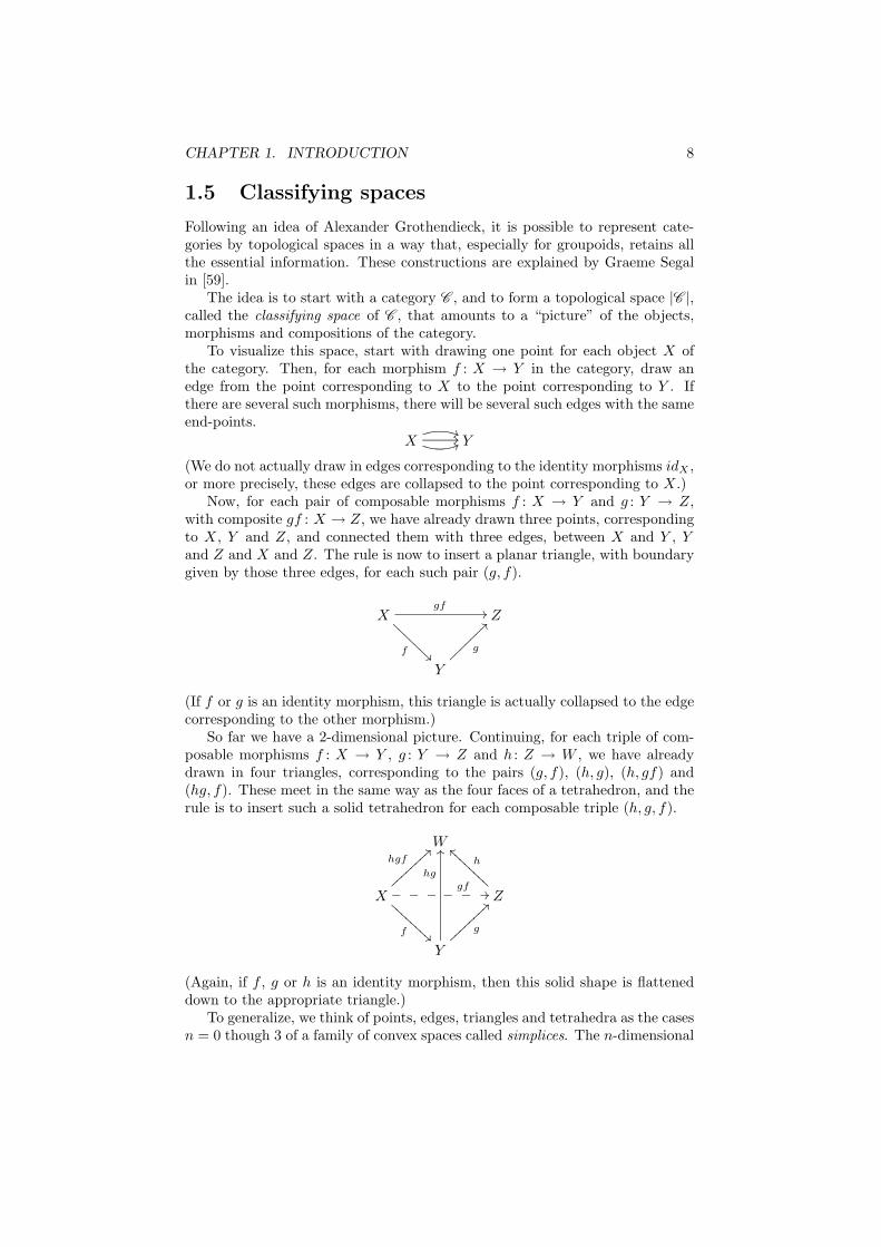
Now, for each pair of composable morphisms f : X → Y and g : Y → Z,with composite gf : X → Z, we have already drawn three points, correspondingto X, Y and Z, and connected them with three edges, between X and Y , Yand Z and X and Z. The rule is now to insert a planar triangle, with boundarygiven by those three edges, for each such pair (g, f).
X
fÃÃ
@@@@
@@@
gf// Z
Y
g
??~~~~~~~
(If f or g is an identity morphism, this triangle is actually collapsed to the edgecorresponding to the other morphism.)
So far we have a 2-dimensional picture. Continuing, for each triple of com-posable morphisms f : X → Y , g : Y → Z and h : Z → W , we have alreadydrawn in four triangles, corresponding to the pairs (g, f), (h, g), (h, gf) and(hg, f). These meet in the same way as the four faces of a tetrahedron, and therule is to insert such a solid tetrahedron for each composable triple (h, g, f).
W
X
fÃÃ
BBBB
BBBB
hgf>>___ gf
//___ Z
h
``AAAAAAAA
Y
g
>>
hg
OO
(Again, if f , g or h is an identity morphism, then this solid shape is flatteneddown to the appropriate triangle.)
To generalize, we think of points, edges, triangles and tetrahedra as the casesn = 0 though 3 of a family of convex spaces called simplices. The n-dimensional
CHAPTER 1. INTRODUCTION 9
simplex ∆n can be taken to be the convex subspace
∆n = (t0, . . . , tn) ∈ In+1 |n∑
i=0
ti = 1
of the (n+1)-cube that is spanned by the (n+1) vertices ei = (0, . . . , 0, 1, 0, . . . , 0)for 0 ≤ i ≤ n. Topologically, ∆n is an n-disc, with boundary ∂∆n homeomor-phic to an (n − 1)-sphere.
At the n-th stage of the construction of C , we insert an n-simplex ∆n foreach n-tuple of composable morphisms (fn, . . . , f1) in C , along a copy of theboundary ∂∆n of the n-simplex, which was already added at the (n−1)-th stage.If any one of the fi is an identity morphism, the n-simplex only appears in asquashed form, already contained in the previous stage. Taking the increasingunion of this sequence of spaces, as n → ∞, we obtain the classifying space |C |.
The precise definition goes in two steps: first one forms a simplicial set N•C
called the nerve of C , with n-simplices NnC the set of n-tuples of composablemorphisms (fn, . . . , f1) in C , and appropriate face and degeneracy maps. Thenone defines the classifying space |C | to be the topological realization of thissimplicial set, given as an identification space
|C | =∐
n≥0
NnC × ∆n/≃ .
We shall return to these constructions later.A key point now is that if C is a groupoid, so that all morphisms are iso-
morphisms, then the classification problem in C becomes a homotopy theoreticquestion about the classifying space |C |. For the isomorphism classes of objectsin C correspond bijectively to the path components of |C |:
π0(C ) ∼= π0(|C |)
and the automorphism group Aut(X) = C (X,X) of any object X in C isisomorphic to the fundamental group of |C | based at the point correspondingto X:
C (X,X) ∼= π1(|C |,X) .
Hence an understanding of the homotopy type of the classifying space |C | issufficient, and in some sense more-or-less equivalent, to an understanding of therefined classification problem in C .
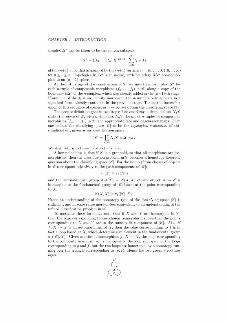
To motivate these formulas, note that if X and Y are isomorphic in C ,then the edge corresponding to any chosen isomorphism shows that the pointscorresponding to X and Y are in the same path component of |C |. Also, iff : X → X is an automorphism of X, then the edge corresponding to f is infact a loop based at X, which determines an element in the fundamental groupπ1(|C |,X). Given another automorphism g : X → X, the loop correspondingto the composite morphism gf is not equal to the loop sum g ∗ f of the loopscorresponding to g and f , but the two loops are homotopic, by a homotopy run-ning over the triangle corresponding to (g, f). Hence the two group structuresagree.
X
f
LL
g
ll
gf
¦¦
CHAPTER 1. INTRODUCTION 10
[[If C is not a groupoid, these formulas fail, but the homotopical data on theright hand side is still of categorical interest.]]
Example 1.5.1. Let iso(Fin) be the groupoid of finite sets and invertible func-tions. The classifying space | iso(Fin)| has one path component for each non-negative integer, with the n-th component containing the point correspondingto the object n = 1, 2, . . . , n. Each permutation σ ∈ Σn specifies a loopin | iso(Fin)| at n, and the fundamental group of that path component is iso-morphic to Σn. It turns out that the universal cover of that path componentis contractible, so that the n-th path component is homotopy equivalent to aspace called BΣn, given by the bar construction on the group Σn. Hence thereis a homotopy equivalence
| iso(Fin)| ≃∐
n≥0
BΣn .
[[Forward reference to bar construction BG for groups (or monoids) G.]]
Exercise 1.5.2. Let G be a finite group, and let iso(G−Fin) be the groupoidof finite G-sets and G-equivariant bijections. Convince yourself that there is ahomotopy equivalence
| iso(G−Fin)| ≃∐
ν
B Aut(X(ν)) ,
where ν ranges over the functions ConjSub(G) → N0. Using Exercise 1.3.3, canyou see that there is a homotopy equivalence
| iso(G−Fin)| ≃∏
(H)
∐
n≥0
B(Σn ≀ WG(H))
where (H) in the product runs through ConjSub(G)? [[Forward reference toSegal–tom Dieck splitting.]]
[[Classifying space of real or complex vector spaces given in terms of Grass-mannians. More elaborate spaces for k-linear G-representations.]]
Example 1.5.3. Let iso(F (R)) be the groupoid of finitely generated free R-modules and R-linear isomorphisms. Under a mild assumption on R, satisfiede.g. if R is commutative or if R = Z[π] is an integral group ring, the classifyingspace | iso(F (R))| has one path component for each non-negative integer, withthe n-th component containing the point corresponding to the object Rn. Eachinvertible matrix A ∈ GLn(R) specifies a loop in | iso(F (R))| at Rn, and thefundamental group of that path component is isomorphic to GLn(R). It againturns out that the universal cover of that path component is contractible, sothat the n-th path component is homotopy equivalent to BGLn(R). Hencethere is a homotopy equivalence
| iso(F (R))| ≃∐
n≥0
BGLn(R) .
In general, for a discrete group G the bar construction BG is a space suchthat its (singular) homology equals the group homology of G, which again canbe expressed as the Tor-groups of the group ring Z[G]:
H∗(BG) ∼= Hgp∗ (G) = TorZ[G]
∗ (Z, Z) .
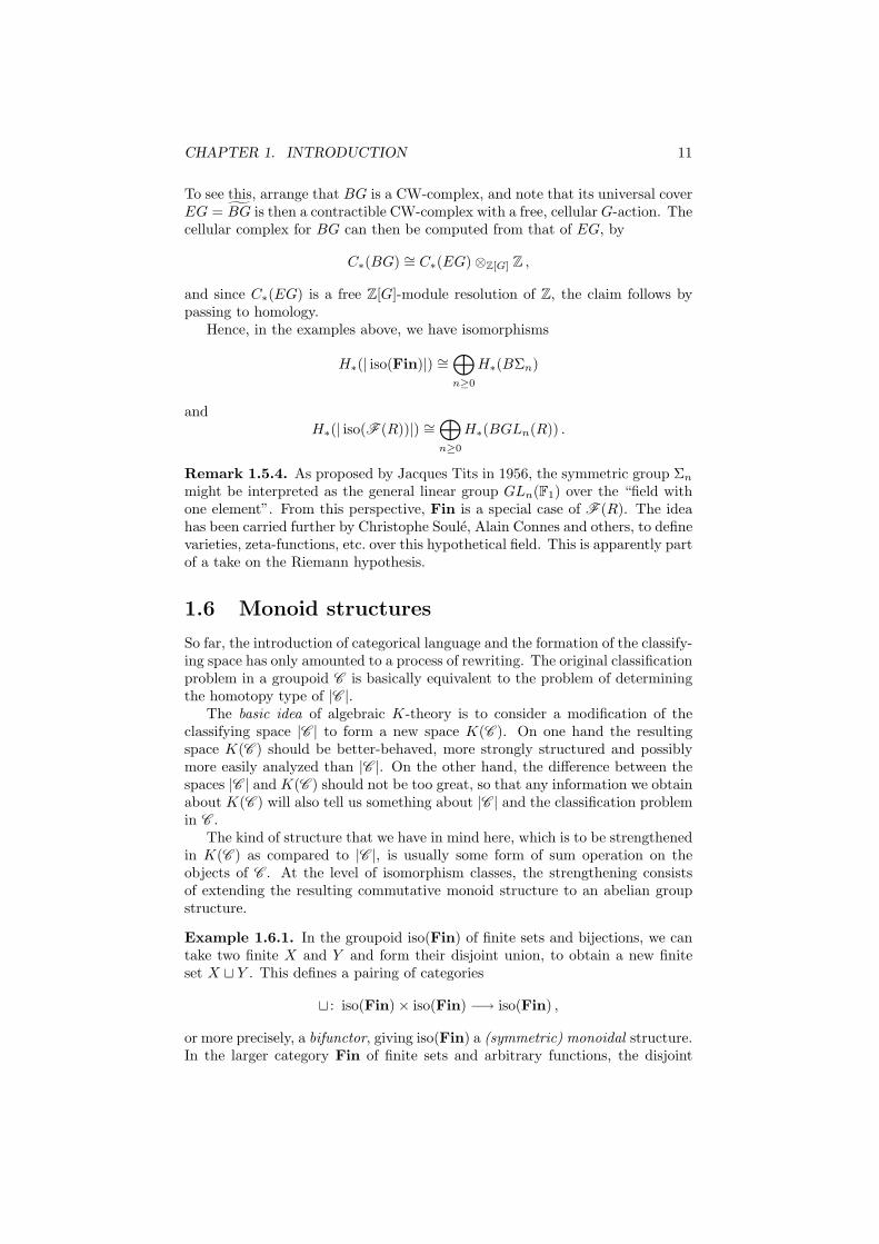
CHAPTER 1. INTRODUCTION 11
To see this, arrange that BG is a CW-complex, and note that its universal coverEG = BG is then a contractible CW-complex with a free, cellular G-action. Thecellular complex for BG can then be computed from that of EG, by
C∗(BG) ∼= C∗(EG) ⊗Z[G] Z ,
and since C∗(EG) is a free Z[G]-module resolution of Z, the claim follows bypassing to homology.
Hence, in the examples above, we have isomorphisms
H∗(| iso(Fin)|) ∼=⊕
n≥0
H∗(BΣn)
andH∗(| iso(F (R))|) ∼=
⊕
n≥0
H∗(BGLn(R)) .
Remark 1.5.4. As proposed by Jacques Tits in 1956, the symmetric group Σn
might be interpreted as the general linear group GLn(F1) over the “field withone element”. From this perspective, Fin is a special case of F (R). The ideahas been carried further by Christophe Soule, Alain Connes and others, to definevarieties, zeta-functions, etc. over this hypothetical field. This is apparently partof a take on the Riemann hypothesis.
1.6 Monoid structures
So far, the introduction of categorical language and the formation of the classify-ing space has only amounted to a process of rewriting. The original classificationproblem in a groupoid C is basically equivalent to the problem of determiningthe homotopy type of |C |.
The basic idea of algebraic K-theory is to consider a modification of theclassifying space |C | to form a new space K(C ). On one hand the resultingspace K(C ) should be better-behaved, more strongly structured and possiblymore easily analyzed than |C |. On the other hand, the difference between thespaces |C | and K(C ) should not be too great, so that any information we obtainabout K(C ) will also tell us something about |C | and the classification problemin C .
The kind of structure that we have in mind here, which is to be strengthenedin K(C ) as compared to |C |, is usually some form of sum operation on theobjects of C . At the level of isomorphism classes, the strengthening consistsof extending the resulting commutative monoid structure to an abelian groupstructure.
Example 1.6.1. In the groupoid iso(Fin) of finite sets and bijections, we cantake two finite X and Y and form their disjoint union, to obtain a new finiteset X ⊔ Y . This defines a pairing of categories
⊔ : iso(Fin) × iso(Fin) −→ iso(Fin) ,
or more precisely, a bifunctor, giving iso(Fin) a (symmetric) monoidal structure.In the larger category Fin of finite sets and arbitrary functions, the disjoint
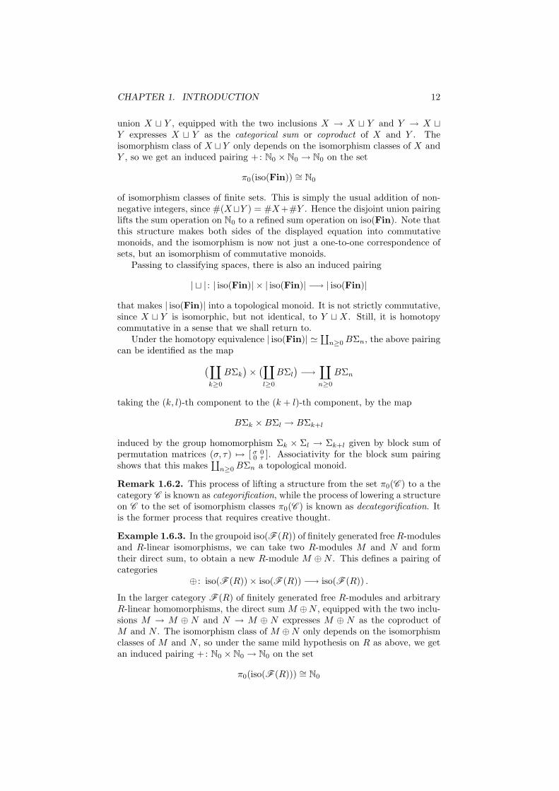
CHAPTER 1. INTRODUCTION 12
union X ⊔ Y , equipped with the two inclusions X → X ⊔ Y and Y → X ⊔Y expresses X ⊔ Y as the categorical sum or coproduct of X and Y . Theisomorphism class of X ⊔ Y only depends on the isomorphism classes of X andY , so we get an induced pairing +: N0 × N0 → N0 on the set
π0(iso(Fin)) ∼= N0
of isomorphism classes of finite sets. This is simply the usual addition of non-negative integers, since #(X⊔Y ) = #X+#Y . Hence the disjoint union pairinglifts the sum operation on N0 to a refined sum operation on iso(Fin). Note thatthis structure makes both sides of the displayed equation into commutativemonoids, and the isomorphism is now not just a one-to-one correspondence ofsets, but an isomorphism of commutative monoids.
Passing to classifying spaces, there is also an induced pairing
| ⊔ | : | iso(Fin)| × | iso(Fin)| −→ | iso(Fin)|
that makes | iso(Fin)| into a topological monoid. It is not strictly commutative,since X ⊔ Y is isomorphic, but not identical, to Y ⊔ X. Still, it is homotopycommutative in a sense that we shall return to.
Under the homotopy equivalence | iso(Fin)| ≃∐
n≥0 BΣn, the above pairingcan be identified as the map
(∐
k≥0
BΣk
)×
(∐
l≥0
BΣl
)−→
∐
n≥0
BΣn
taking the (k, l)-th component to the (k + l)-th component, by the map
BΣk × BΣl → BΣk+l
induced by the group homomorphism Σk × Σl → Σk+l given by block sum ofpermutation matrices (σ, τ) 7→ [ σ 0
0 τ ]. Associativity for the block sum pairingshows that this makes
∐n≥0 BΣn a topological monoid.
Remark 1.6.2. This process of lifting a structure from the set π0(C ) to a thecategory C is known as categorification, while the process of lowering a structureon C to the set of isomorphism classes π0(C ) is known as decategorification. Itis the former process that requires creative thought.
Example 1.6.3. In the groupoid iso(F (R)) of finitely generated free R-modulesand R-linear isomorphisms, we can take two R-modules M and N and formtheir direct sum, to obtain a new R-module M ⊕ N . This defines a pairing ofcategories
⊕ : iso(F (R)) × iso(F (R)) −→ iso(F (R)) .
In the larger category F (R) of finitely generated free R-modules and arbitraryR-linear homomorphisms, the direct sum M ⊕N , equipped with the two inclu-sions M → M ⊕ N and N → M ⊕ N expresses M ⊕ N as the coproduct ofM and N . The isomorphism class of M ⊕N only depends on the isomorphismclasses of M and N , so under the same mild hypothesis on R as above, we getan induced pairing +: N0 × N0 → N0 on the set
π0(iso(F (R))) ∼= N0
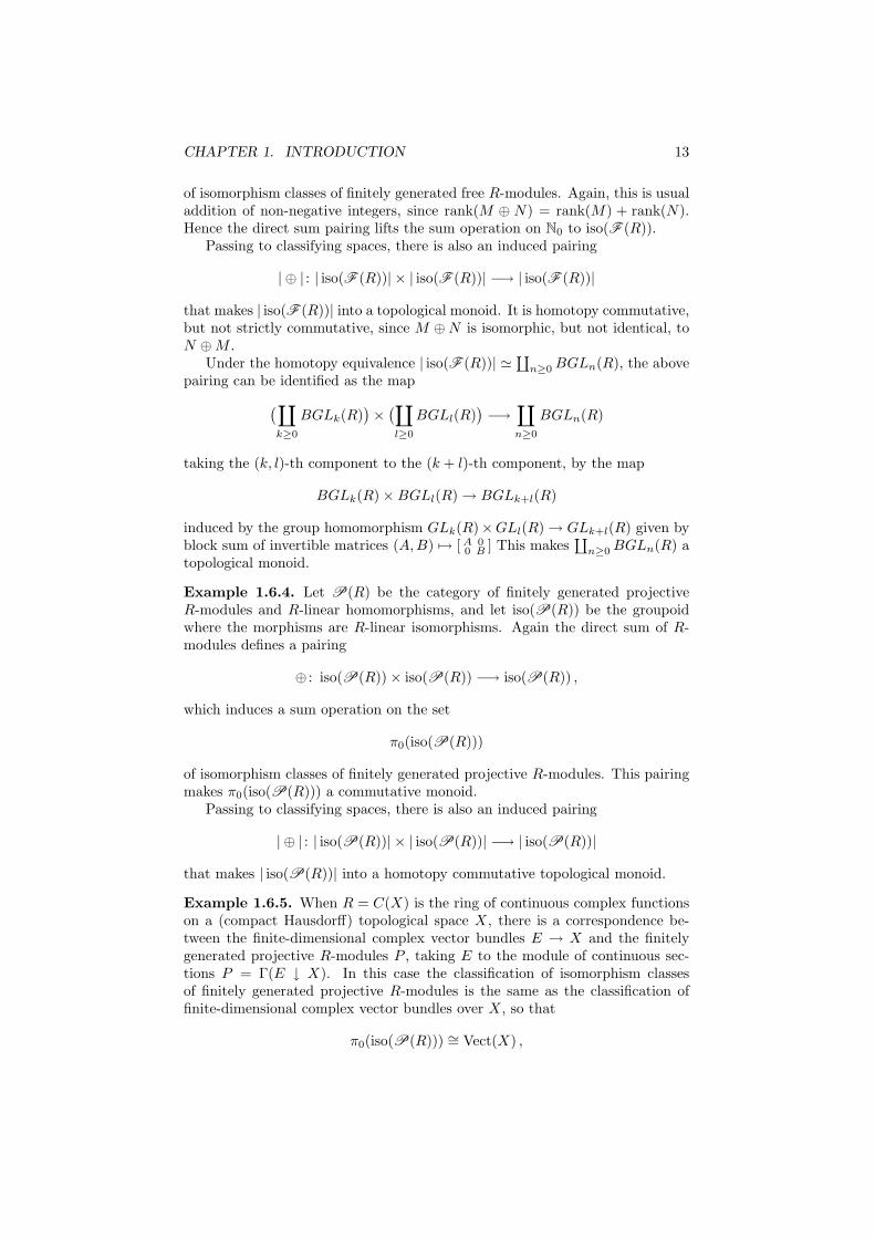
CHAPTER 1. INTRODUCTION 13
of isomorphism classes of finitely generated free R-modules. Again, this is usualaddition of non-negative integers, since rank(M ⊕ N) = rank(M) + rank(N).Hence the direct sum pairing lifts the sum operation on N0 to iso(F (R)).
Passing to classifying spaces, there is also an induced pairing
| ⊕ | : | iso(F (R))| × | iso(F (R))| −→ | iso(F (R))|
that makes | iso(F (R))| into a topological monoid. It is homotopy commutative,but not strictly commutative, since M ⊕ N is isomorphic, but not identical, toN ⊕ M .
Under the homotopy equivalence | iso(F (R))| ≃∐
n≥0 BGLn(R), the abovepairing can be identified as the map
(∐
k≥0
BGLk(R))×
(∐
l≥0
BGLl(R))−→
∐
n≥0
BGLn(R)
taking the (k, l)-th component to the (k + l)-th component, by the map
BGLk(R) × BGLl(R) → BGLk+l(R)
induced by the group homomorphism GLk(R)×GLl(R) → GLk+l(R) given byblock sum of invertible matrices (A,B) 7→ [ A 0
0 B ] This makes∐
n≥0 BGLn(R) atopological monoid.
Example 1.6.4. Let P(R) be the category of finitely generated projectiveR-modules and R-linear homomorphisms, and let iso(P(R)) be the groupoidwhere the morphisms are R-linear isomorphisms. Again the direct sum of R-modules defines a pairing
⊕ : iso(P(R)) × iso(P(R)) −→ iso(P(R)) ,
which induces a sum operation on the set
π0(iso(P(R)))
of isomorphism classes of finitely generated projective R-modules. This pairingmakes π0(iso(P(R))) a commutative monoid.
Passing to classifying spaces, there is also an induced pairing
| ⊕ | : | iso(P(R))| × | iso(P(R))| −→ | iso(P(R))|
that makes | iso(P(R))| into a homotopy commutative topological monoid.
Example 1.6.5. When R = C(X) is the ring of continuous complex functionson a (compact Hausdorff) topological space X, there is a correspondence be-tween the finite-dimensional complex vector bundles E → X and the finitelygenerated projective R-modules P , taking E to the module of continuous sec-tions P = Γ(E ↓ X). In this case the classification of isomorphism classesof finitely generated projective R-modules is the same as the classification offinite-dimensional complex vector bundles over X, so that
π0(iso(P(R))) ∼= Vect(X) ,

CHAPTER 1. INTRODUCTION 14
where Vect(X) denotes the set of isomorphism classes of such vector bundles.This is an isomorphism of commutative monoids, where the direct sum of R-modules on the left corresponds to the Whitney sum of vector bundles on theright. For example, when X = Sk+1, Vect(Sk+1) is the disjoint union over n ≥ 0of the homotopy groups πk(U(n)), which are not all known. This shows that thestructure of π0(iso(P(R))) can in general be rather complicated. [[Reference toSerre and Swan?]]
1.7 Group completion
Note that the monoids N0 and π0(iso(P(R))) are not groups, since most ele-ments lack additive inverses, or negatives. After all, there are no sets with anegative number of elements, and no R-modules of negative rank.
A fundamental idea of Grothendieck was to strengthen the algebraic struc-ture on commutative monoids, like π0(C ), by adjoining additive inverses to allits elements, so as to obtain an actual abelian group.
Algebraically, this is an easy construction. Given a commutative monoidM , written additively with neutral element 0, view elements (a, b) of M ×M asformal differences a− b, by introducing the equivalence relation (a, b) ∼ (c, d) ifthere exists an f ∈ M such that a + d + f = b + c + f . (If the cancellation lawx + f = y + f =⇒ x = y holds in M , one may omit all mention of f .) Thenthe set of equivalence classes
K(M) = (M × M)/∼
becomes an abelian group, with componentwise sum. The negative of the equiv-alence class [a, b] of (a, b) is [b, a], and there is a monoid homomorphism
ι : M → K(M)
that takes a to [a, 0]. In a precise sense this is the initial monoid homomorphismfrom M to any abelian group, so K(M) is the group completion of M . Forexample, K(N0) ∼= Z. We also call K(M) the Grothendieck group of M .
Example 1.7.1. Let G be a finite group, and let M(G) = π0(iso(G−Fin))be the commutative monoid of isomorphism classes of finite G-sets, with sumoperation [X]+ [Y ] = [X ⊔Y ] induced by disjoint union. Let A(G) = K(M(G))be the associated Grothendieck group. The identification of M(G) with theset of functions ν : ConjSub(G) → N0 is compatible with the sum operation(defined pointwise by (ν + µ)(H) = ν(H) + µ(H)), since X(ν) ⊔ X(µ) ∼=X(ν + µ). Hence A(G) = K(M(G)) is isomorphic to the abelian group offunctions ν : ConjSub(G) → Z. From another point of view, M(G) is the freecommutative monoid generated by the isomorphism classes of transitive G-setsG/H, and A(G) is the free abelian group generated by the same isomorphismclasses.
The abelian group A(G) has a natural commutative ring structure, and istherefore known as the Burnside ring. (Another common notation is Ω(G).)The cartesian product X × Y of two finite G-sets X and Y is again a finiteG-set, with the diagonal G-action g · (x, y) = (g · x, g · y), and this pairingM(G)×M(G) → M(G) extends to the ring product A(G)×A(G) → A(G). By
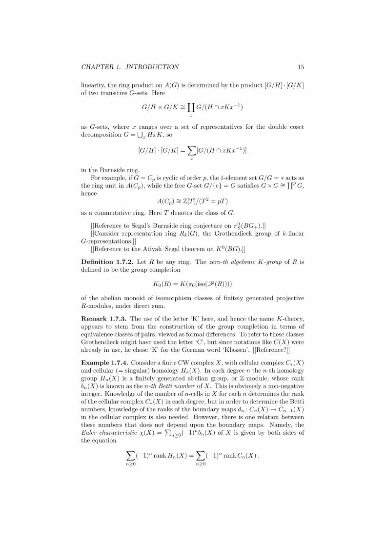
CHAPTER 1. INTRODUCTION 15
linearity, the ring product on A(G) is determined by the product [G/H] · [G/K]of two transitive G-sets. Here
G/H × G/K ∼=∐
x
G/(H ∩ xKx−1)
as G-sets, where x ranges over a set of representatives for the double cosetdecomposition G =
⋃x HxK, so
[G/H] · [G/K] =∑
x
[G/(H ∩ xKx−1)]
in the Burnside ring.For example, if G = Cp is cyclic of order p, the 1-element set G/G = ∗ acts as
the ring unit in A(Cp), while the free G-set G/e = G satisfies G×G ∼=∐p
G,hence
A(Cp) ∼= Z[T ]/(T 2 = pT )
as a commutative ring. Here T denotes the class of G.
[[Reference to Segal’s Burnside ring conjecture on π0S(BG+).]]
[[Consider representation ring Rk(G), the Grothendieck group of k-linearG-representations.]]
[[Reference to the Atiyah–Segal theorem on K0(BG).]]
Definition 1.7.2. Let R be any ring. The zero-th algebraic K-group of R isdefined to be the group completion
K0(R) = K(π0(iso(P(R))))
of the abelian monoid of isomorphism classes of finitely generated projectiveR-modules, under direct sum.
Remark 1.7.3. The use of the letter ‘K’ here, and hence the name K-theory,appears to stem from the construction of the group completion in terms ofequivalence classes of pairs, viewed as formal differences. To refer to these classesGrothendieck might have used the letter ‘C’, but since notations like C(X) werealready in use, he chose ‘K’ for the German word ‘Klassen’. [[Reference?]]
Example 1.7.4. Consider a finite CW complex X, with cellular complex C∗(X)and cellular (= singular) homology H∗(X). In each degree n the n-th homologygroup Hn(X) is a finitely generated abelian group, or Z-module, whose rankbn(X) is known as the n-th Betti number of X. This is obviously a non-negativeinteger. Knowledge of the number of n-cells in X for each n determines the rankof the cellular complex C∗(X) in each degree, but in order to determine the Bettinumbers, knowledge of the ranks of the boundary maps dn : Cn(X) → Cn−1(X)in the cellular complex is also needed. However, there is one relation betweenthese numbers that does not depend upon the boundary maps. Namely, theEuler characteristic χ(X) =
∑n≥0(−1)nbn(X) of X is given by both sides of
the equation
∑
n≥0
(−1)n rankHn(X) =∑
n≥0
(−1)n rankCn(X) .
CHAPTER 1. INTRODUCTION 16
Of course, this is now an equation that takes place in Z, not in N0, even if eachindividual rank is non-negative.
As a consequence, the Euler characteristic satisfies some useful relations ina number of cases. For example, if Y → X is a k-fold covering space, thenχ(Y ) = k · χ(X), since there are k n-cells in Y covering each n-cell in X, sorankCn(Y ) = k · rankCn(X). More generally, if F → E → B is a fiber bundle(or fibration) with F , E and B finite CW complexes then χ(E) = χ(B) · χ(F ).In general there is no equally simple relation between the Betti numbers, sincethere may be many differentials in the Serre spectral sequence
E2∗,∗ = H∗(B;H∗(F )) =⇒ H∗(E) .
The point to note is that in order to make use of the Euler characteristic, inplace of Betti numbers, we have to work with integers instead of non-negativeintegers.
1.8 Loop space completion
The fundamental idea of higher algebraic K-theory, as created by Quillen, is tostrengthen the algebraic structure on topological monoids, like |C |, by topolog-ically adjoining homotopy inverses in a systematic manner, along a map
ι : |C | → K(C ) .
The well-behaved way of specifying this is a topological process of loop spacecompletion, since loop spaces have homotopy inverses realized by reversing thedirection of travel around a loop. In this case the details of the definitionrequire more topological sophistication than in the algebraic definition of K0.The algebraic construction and the higher, topological one, will be compatibleafter decategorification, in the sense that
K(π0(C )) ∼= π0(K(C )) .
[[Sometimes we give a sum structure on π0(C ) by setting [X] + [Y ] = [Z]whenever there is a suitable extension 0 → X → Z → Y → 0, not just whenZ = X ⊕ Y . Then the starting data on |C | is more than just the monoidstructure induced by | ⊕ |, and K(C ) is not just the group completion of thatmonoid structure.]]
[[In the case of Waldhausen’s S• construction, the starting data is given bya category with cofibrations and weak equivalences. In the case of Quillen’sQ-construction, this is specialized to an exact category.]]
In the examples discussed in Section 1.6, where a pairing ⊕ : C × C → C
makes M = |C | a topological monoid, and we seek to group complete π0(C )with respect to the induced sum operation, the algebraic K-theory space K(C )can be constructed as a loop space using the bar construction BM for monoids:
K(C ) = ΩB|C | .
For any based space X, ΩX = Map∗(S1,X) denotes the loop space of X, defined
as the space of based maps from S1 to X. There is an inclusion Σ|C | → B|C |,where ΣX = X ∧ S1 denotes the suspension of X. There is a natural mapX → ΩΣX that maps x to the loop s 7→ x ∧ s, and the group completion mapι : |C | → K(C ) factors as |C | → ΩΣ|C | → ΩB|C |.
CHAPTER 1. INTRODUCTION 17
Definition 1.8.1. The higher algebraic K-groups of C are in this case definedas the homotopy groups
Ki(C ) = πi(K(C ))
of the loop space K(C ), for i ≥ 0. In particular, for each ring R we let K(R) =K(iso(P(R))) and Ki(R) = πi(K(R)).
Under similar hypotheses [[forward reference]], the amazing thing happensthat K(C ) is not just a loop space, i.e., a space of the form ΩX1, but it is aninfinite loop space, i.e., there is a sequence of spaces Xn such that Xn ≃ ΩXn+1
for all n ≥ 0, and K(C ) = X0. In particular, K(C ) ≃ ΩnXn = Map∗(Sn,Xn)
is an n-fold loop space, for each n ≥ 0. The sequence of spaces K(C ) =Xnn≥0 form a spectrum in the sense of algebraic topology, or equivalently, anS-module, where S is the sphere spectrum. In this sense, K(C ) is a much morestrongly structured object than the classifying space |C |, and this additionalstructure can often be brought to bear on the identification and the analysis ofits homotopy type.
For this to be useful for the original classification question in C , we mustof course know something about the group completion map ι. Here there is nogeneral theorem, but in many special cases there are particular results abouthow close |C | and K(C ) are. We shall review some of these results in the restof this chapter.
1.9 Grothendieck–Riemann–Roch
The zero-th K-groups were introduced by Grothendieck around 1956 in thecontext of sheaves over algebraic varieties, see [6] for the published expositionby Borel and Serre. In general there are two K-groups associated to a varietyX, here denoted K0(X) and K ′
0(X), but they are isomorphic for X smooth andquasi-projective.
The abelian group K ′0(X) is defined to be generated by the set π0(Coh(X))
of isomorphism classes [F ] of coherent sheaves over X, subject to the relation
[F ] = [F ′] + [F ′′]
whenever0 → F
′ → F → F′′ → 0
is a short exact sequence of coherent sheaves. Note that in this case, we may ormay not have that F is isomorphic to the direct sum F ′ ⊕ F ′′. Some authorswrite G0(X) for the Grothendieck group K ′
0(X)The abelian group K0(X) is defined to be generated by the set of isomor-
phism classes [F ] of algebraic vector bundles over X, subject to the same re-lation as above. However, in this case each short exact sequence of vectorbundles admits a splitting, so the relation may also be expressed as saying that[F ] = [F ′] + [F ′′] whenever F ∼= F ′ ⊕ F ′′.
Each vector bundle is a coherent sheaf, so there is a natural homomor-phism K0(X) → K ′
0(X), and this is an isomorphism when X is smooth andquasi-projective, essentially because each coherent sheaf admits a finite lengthresolution by vector bundles. We shall generalize this in the resolution theorem[[forward reference]].
CHAPTER 1. INTRODUCTION 18
In the affine case, when X = Spec(R), the category Coh(X) of coherentsheaves over X is equivalent to the category M (R) of finitely generated R-modules, and the category of vector bundles over X is equivalent to the cate-gory P(R) of finitely generated projective R-modules. In particular, K0(X) =K0(R).
Grothendieck proves the Riemann–Roch theorem in a relative form, startingwith a proper morphism f : X → Y of smooth and quasi-projective varieties.The direct image functor f∗ has right derived functors Rqf∗ for all q ≥ 0, andGrothendieck shows that for each coherent sheaf F over X, each derived directimage (Rqf∗)(F ) is a coherent sheaf over Y . The correct statement of theRiemann–Roch theorem is not just about the direct image homomorphism (ofcommutative monoids)
f∗ : π0(Coh(X)) → π0(Coh(Y ))
taking [F ] to [f∗(F )], but about the total derived direct image homomorphism
f! =∑
q≥0
(−1)q(Rqf∗) .
As in the case of Euler characteristics, the alternating sum f!(F ) cannot be as-sumed to take values in π0(Coh(Y )), but it does make sense in the Grothendieckgroup K ′
0(Y ). Having done this, it is easy to see that f! is additive on extensionsof coherent sheaves, so that it defines a homomorphism (of abelian groups)
f! : K ′0(X) → K ′
0(Y ) .
This maneuver is therefore needed to even state the Grothendieck–Riemann–Roch theorem, which compares the total derived direct image f! with the cor-responding direct image f∗ : A(X) → A(Y ) of Chow groups, via the Cherncharacter ch : K0(X) → A(X)⊗Q. The direct images do not directly agree, butthey do when multiplied by the so-called Todd class td(X) ∈ A(X) ⊗ Q. Thegeneral formula reads:
ch(f!(F )) · td(Y ) = f∗(ch(F ) · td(X))
When X is smooth and projective of dimension n, the unique map f : X → Y =Spec(k) is proper, and the formula specializes to
χ(X,F ) = (ch(F ) · td(X))n ,
where the subscript n refers to the degree n part. [[Explain, or use Kroneckerpairing with fundamental class [X]?]] In the case k = C of complex varieties,this is the Hirzebruch–Riemann–Roch theorem, and when n = 1, one recoversthe classical Riemann–Roch theorem for complex algebraic curves.
1.10 Vector fields on spheres
For each n ≥ 1, the following statements are equivalent:
(a) There is a division algebra over R of dimension n;
CHAPTER 1. INTRODUCTION 19
(b) The sphere Sn−1 admits (n− 1) tangent vector fields that are everywherelinearly independent;
(c) There is a two-cell complex X = Sn ∪f D2n in which the cup productsquare of a generator of Hn(X; Z/2) is a generator of H2n(X; Z/2).
The division algebras R, C, H (the quaternions) and O (the octonions) showthat these statements are true for n = 1, 2, 4 and 8.
It is a theorem of Frank Adams [1] from 1960 that the third statement is falsefor all other values of n. In particular, there are no higher-dimensional divisionalgebras then the ones given. Adams’ original proof used a factorization of theSteenrod operations Sqn in singular cohomology (for n a power of two) usingsecondary cohomology operations, and is rather delicate.
Following Grothendieck’s ideas from algebraic geometry, Michael Atiyah andFriedrich Hirzebruch [4] introduced topological K-theory in 1959. For a finiteCW complex X, the group
K0(X) = K(Vect(X))
is defined to be the Grothendieck group of the commutative monoid of isomor-phism classes of finite-dimensional complex vector bundles over X. A few yearslater, Adams and Atiyah [2] found a quick and short, so-called “postcard proof”,of Adams’ theorem, replacing the use of singular cohomology, Steenrod opera-tions and secondary cohomology operations by the use of topological K-theoryand the much simpler Adams operations ψk : K0(X) → K0(X).
For expositions of the K-theory proof, see Husemoller [28, Ch. 14] or Sec-tion 2.3 of Allen Hatcher’s book project
http://www.math.cornell.edu/∼hatcher/VBKT/VBpage.html .
1.11 Wall’s finiteness obstruction
Here is a more elaborate version of Example 1.7.4. Suppose for simplicity thatX is a path-connected CW complex, with universal covering space p : X → X.Fix a base point in X, and let π = π1(X) be the fundamental group. Then π
acts freely by deck transformations on X. The CW structure on X lifts to a CWstructure on X, and π permutes the cells of X freely. Hence the cellular complexC∗(X) of X is a complex of free Z[π]-modules. Since X is the orbit space for the
free π-action on X, we have the isomorphism C∗(X) ∼= Z⊗Z[π]C∗(X) previouslymentioned.
If X is a finite CW complex, then there are finitely many free π-orbits of cellsin X, and C∗(X) is a bounded complex of finitely generated free Z[π]-modules.
In other words, each Cn(X) is a finitely generated free Z[π]-module, which is
nonzero only for finitely many n. For each n the isomorphism class of Cn(X)therefore defines an element in the commutative monoid
π0(iso(F (Z[π])))
which we may map, by viewing free modules as projective, to the commutativemonoid
π0(iso(P(Z[π]))) .
CHAPTER 1. INTRODUCTION 20
Now, the precise cellular modules C∗(X) depend on the particular choice of CWstructure on X. However, as for the Euler characteristic above, the alternatingsum
[X] =∑
n≥0
(−1)n[Cn(X)] ∈ K0(Z[π])
is in fact independent of the CW structure. Of course, in order to form this alter-nating sum [X], we had to go from the commutative monoid π0(iso(P(Z[π])))to its group completion K0(Z[π]).
In this case the added complexity does not tell us something new. Afterall, if X has cn n-cells, then Cn(X) is the free Z-module on cn generators
and Cn(X) is the free Z[π]-module on equally many generators. Hence we can
obtain Cn(X) from Cn(X) by base change along the unique ring homomorphism
Z → Z[π]. (This only works one degree at a time. The boundary maps in C∗(X)are usually not induced up from those in C∗(X).) It follows that the alternatingsum [X] ∈ K0(Z[π]) is the image of the ordinary Euler characteristic χ(X) ∈ Z,under the natural map
Z ∼= K0(Z) → K0(Z[π])
that takes an integer c to the class of the Z-module Zc, and then to the Z[π]-module Z[π]c.
Definition 1.11.1. Let R be any ring. The projective class group K0(R) isthe cokernel of the natural homomorphism K0(Z) → K0(R), or equivalently,the quotient of K0(R) by the subgroup generated by R viewed as a finitelygenerated free, hence projective, R-module of rank 1.
Here is an extension of the previous example, due to Terry Wall [71] from
1965, which involves the projective class group K0(Z[π]) in a much more es-sential way. A first step towards the classification of compact manifolds is todetermine which homotopy types of spaces are realized by manifolds. A secondstep is then to determine how many different manifolds there are of the samehomotopy type, and a third step is to understand the symmetries of each ofthese manifolds.
Staying with the first step, every compact manifold M can be embedded insome Euclidean space Rk, and is then a retract of some open neighborhood in Rk.Such a space is called an Euclidean neighborhood retract, abbreviated ENR.Each compact ENR is a retract of a finite simplicial complex, hence of a finiteCW complex. See [26, App. A] for proofs of these results. So when searchingfor manifolds, we need only consider those homotopy types of spaces that arehomotopy equivalent to retracts of finite CW complexes. It is convenient torelax the ‘retraction’ condition as follows.
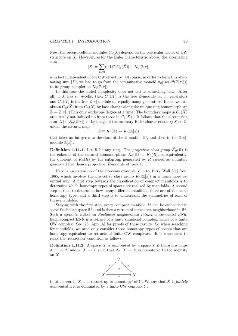
Definition 1.11.2. A space X is dominated by a space Y if there are mapsd : Y → X and s : X → Y such that ds : X → X is homotopic to the identityon X.
Yd
ÃÃ@@
@@@@
@
≃
X =//
s
>>~~~~~~~X
In other words, X is a ‘retract up to homotopy’ of Y . We say that X is finitelydominated if it is dominated by a finite CW complex Y .
CHAPTER 1. INTRODUCTION 21
It is known that all compact manifolds are homotopy equivalent to finiteCW complexes. This is clear for piece-wise linear manifolds (since these admita triangulation as a finite simplicial complex), hence also for smooth manifolds,but is a deep fact due to Rob Kirby and Larry Siebenmann [34] for topologicalmanifolds.
This leads to the question whether a finitely dominated space X, i.e., aspace dominated by a finite CW complex, must itself be homotopy equivalentto a finite CW complex. The answer is ‘yes’ for simply-connected X, as followsfrom [26, Prop. 4C.1]. However, for general X the answer involves an element
in the projective class group K0(Z[π]), known as Wall’s finiteness obstruction.
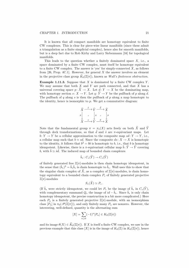
Example 1.11.3. Suppose that X is dominated by a finite CW complex Y .We may assume that both X and Y are path connected, and that X has auniversal covering space p : X → X. Let d : Y → X be the dominating map,with homotopy section s : X → Y . Let q : Y → Y be the pullback of p along d.The pullback of q along s is then the pullback of p along a map homotopic tothe identity, hence is isomorphic to p. We get a commutative diagram:
Xs //
p
²²
y
Yd //
q
²²
y
X
p
²²
Xs // Y
d // X
Note that the fundamental group π = π1(X) acts freely on both X and Ythrough deck transformations, so that d and s are π-equivariant maps. Letb : Y → Y be a cellular approximation to the composite map sd : Y → Y , i.e.,a cellular map such that b ≃ sd. Since the composite ds : X → X is homotopicto the identity, it follows that b2 = bb is homotopic to b, i.e., that b is homotopyidempotent. Likewise, there is a π-equivariant cellular map b : Y → Y coveringb, with b ≃ sd. The induced map of bounded chain complexes
b∗ : C∗(Y ) → C∗(Y )
of finitely generated free Z[π]-modules is then chain homotopy idempotent, inthe sense that (b∗)
2 = b∗b∗ is chain homotopic to b∗. Wall uses this to show that
the singular chain complex of X, as a complex of Z[π]-modules, is chain homo-topy equivalent to a bounded chain complex P∗ of finitely generated projectiveZ[π]-modules
S∗(X) ≃ P∗ .
(If b∗ were strictly idempotent, we could let P∗ be the image of b∗ in C∗(Y ),with complementary summand Q∗ the image of id − b∗. Since b∗ is only chainhomotopy idempotent, the precise construction is a bit more complicated.) Hereeach Pn is a finitely generated projective Z[π]-module, with an isomorphismclass [Pn] in π0(P(Z[π])), and only finitely many Pn are nonzero. However, theinteresting, well-defined, quantity is the alternating sum
[X] =∑
n≥0
(−1)n[Pn] ∈ K0(Z[π])
and its image θ(X) ∈ K0(Z[π]). If X is itself a finite CW complex, we saw in theprevious example that this class [X] is in the image of K0(Z) in K0(Z[π]), hence
CHAPTER 1. INTRODUCTION 22
maps to zero in the projective class group K0(Z[π]). Wall’s theorem in this con-text is that the converse holds: a finitely dominated X is homotopy equivalentto a finite CW complex if and only if the class θ(X) is zero in K0(Z[π]). Thisclass is therefore called Wall’s finiteness obstruction. For our purposes, themain thing to note is that this theorem requires the zero-th algebraic K-groupto form the alternating sum [X], which maps to the finiteness obstruction θ(X)in the projective class group. For further references, the survey [19] may be agood place to start.
1.12 Homology of linear groups
Recall the homotopy equivalence
| iso(F (R))| ≃∐
n≥0
BGLn(R)
and the induced isomorphism
H∗(| iso(F (R))|) ∼=⊕
n≥0
H∗(BGLn(R)) .
One way to understand the group homology of the general linear groups GLn(R)is thus to understand the homology of the classifying space of the groupoidF (R).
There is a stabilization homomorphism GLn(R) → GLn+1(R) given by blocksum A 7→ [ A 0
0 1 ] with the 1 × 1 matrix [1] ∈ GL1(R). We let GL∞(R) =colimn GLn(R) be the increasing union of all of the finite GLn(R). The elementsof GL∞(R) are infinite matrices with entries in R, that agree with the identitymatrix except in finitely many places. Applying bar constructions, there arestabilization maps BGLn(R) → BGLn+1(R) for all n, and
BGL∞(R) = colimn
BGLn(R)
is the increasing union of all of these spaces.After passage to loop space completion, along the map
ι :∐
n≥0
BGLn(R) → K(iso(F (R))) ,
the block sum with [1] becomes homotopy invertible. It follows that ι factorsas a composite
∐
n≥0
BGLn(R)α
−→ Z × BGL∞(R)β
−→ K(iso(F (R))) ,
where α is the natural inclusion that takes BGLn(R) to n×BGL∞(R). By thehomology fibration theorem of Dusa McDuff and Graeme Segal [46], or Quillen’s“Q = +” theorem, presented by Daniel Grayson in [23], the second map β is ahomology isomorphism. Furthermore, each path component of K(iso(F (R)))is homotopy equivalent to the base point path component K(R)0 of K(R) =K(iso(P(R))). Hence
β∗ : H∗(BGL∞(R))∼=−→ H∗(K(R)0)
CHAPTER 1. INTRODUCTION 23
is an isomorphism, This means that if we can identify the (infinite) loop spaceK(R) and compute its homology, then we have also computed the homology ofthe infinite general linear group GL∞(R).
It then remains to understand the effect of α in homology. It turns out that,for many reasonable rings R, the stabilization GLn(R) → GLn+1(R) induceshomomorphisms
Hi(BGLn(R)) → Hi(BGLn+1(R))
that are isomorphisms for i in a range that grows to infinity with n. See Charney[10] for one such result, which applies when R is a Dedekind domain. Hence,for i in this stable range, there are isomorphisms Hi(BGLn(R)) ∼= Hi(K(R)0).
Example 1.12.1. [[R = C with the usual topology, with BLn(C) ≃ BU(n)homotopy equivalent to the Grassmannian Grn(C∞) of complex n-dimensionalsubspaces in C∞, and K-theory space Z × BU .]]
Example 1.12.2. This method was successfully applied by Quillen [54] in thecase when R = Fq is a finite field with q = pd elements, and his definition of thehigher algebraic K-groups was motivated by this approach.
Quillen first relates the base point component K(Fq)0 to the infinite Grass-mannian BU , and the homotopy fixed-points Fψq for the Adams operationψq : BU → BU . For each prime ℓ 6= p, this lets him calculate its homologyalgebra (implicitly with coefficients in Z/ℓ) as
H∗(BGL∞(Fq)) ∼= P (ξ1, ξ2, . . . ) ⊗ E(η1, η2, . . . ) ,
where deg(ξj) = 2jr, deg(ηj) = 2jr− 1, r is the least natural number such thatℓ | qr − 1, and P and E denote the polynomial algebra and the exterior algebraon the given generators, respectively. Then he goes on to study α∗, and findsthat it is injective, with image
⊕
n≥0
H∗(BGLn(Fq)) ∼= P (ǫ, ξ1, ξ2, . . . ) ⊗ E(η1, η2, . . . ) ,
where ǫ ∈ H0(GL1(Fq)) is the class of [1], ξj ∈ H2jr(GLr(Fq)) and ηj ∈H2jr−1(GLr(Fq)). From this, each individual group H∗(BGLn(Fq)) can beextracted.
In the case of (implicit) Z/p-coefficients, the results are less complete, butin the limiting case
Hi(BGL∞(Fq)) = 0
for all i > 0, so it follows by homological stability that Hi(BGLn(Fq); Z/p) = 0for all n sufficiently large compared to i.
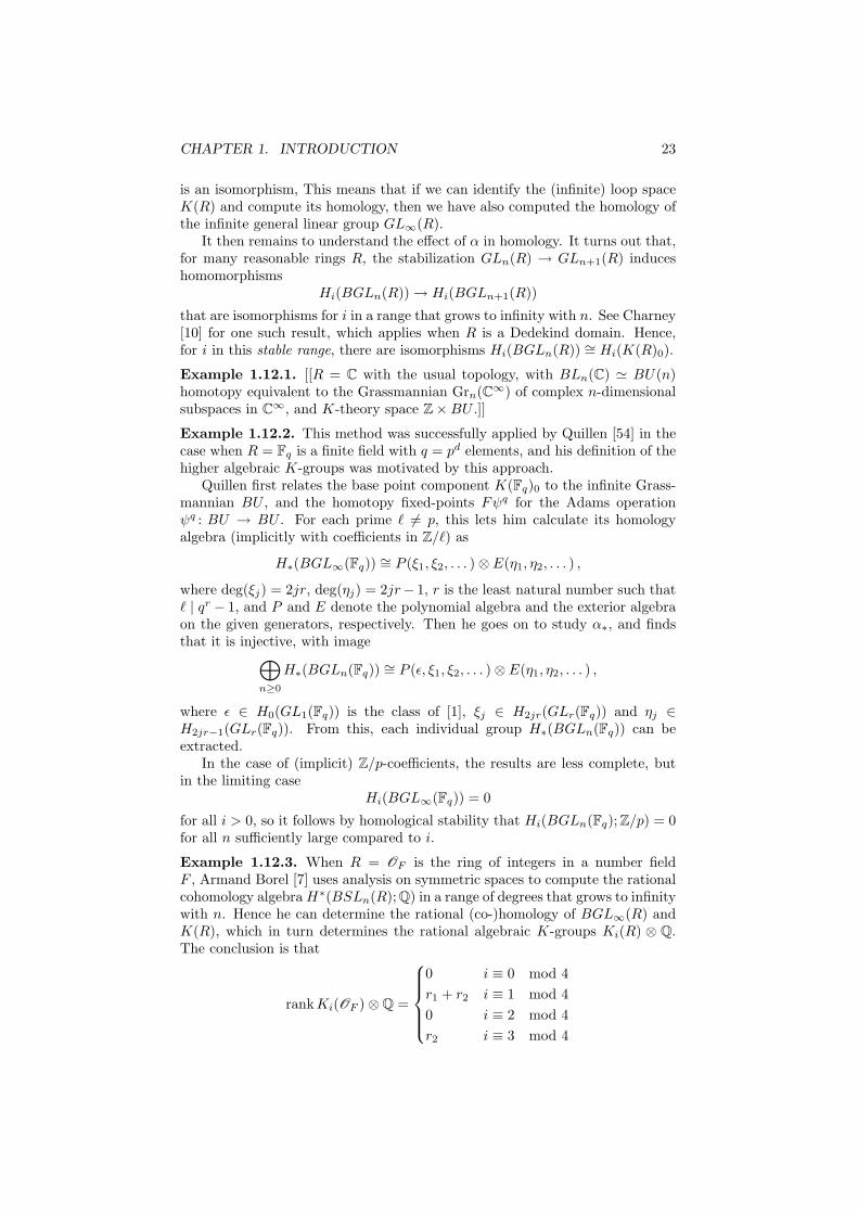
Example 1.12.3. When R = OF is the ring of integers in a number fieldF , Armand Borel [7] uses analysis on symmetric spaces to compute the rationalcohomology algebra H∗(BSLn(R); Q) in a range of degrees that grows to infinitywith n. Hence he can determine the rational (co-)homology of BGL∞(R) andK(R), which in turn determines the rational algebraic K-groups Ki(R) ⊗ Q.The conclusion is that
rankKi(OF ) ⊗ Q =
0 i ≡ 0 mod 4
r1 + r2 i ≡ 1 mod 4
0 i ≡ 2 mod 4
r2 i ≡ 3 mod 4
CHAPTER 1. INTRODUCTION 24
for i ≥ 2, where r1 and r2 are the number of real and complex places of F ,respectively. For example, when F = Q, R = Z and i ≥ 2 the rank of Ki(Z)⊗Q
is one for i ≡ 1 mod 4 and zero otherwise.Furthermore, by a theorem of Quillen [56], which rests on a duality theorem
of Borel–Serre and finiteness theorems of Ragunathan, each group Ki(OF ) isfinitely generated. Hence, for i ≥ 2 each group Ki(Z) is the sum of a copy of Z
and a finite group for i ≡ 1 mod 4, and is a finite group otherwise.[[Also results for rings of integers in local fields, group rings of finite groups.]]
Example 1.12.4. When R = OF [1/p] is the ring of p-integers in a local orglobal number field F , Bill Dwyer and Steve Mitchell [15, §10] have been ableto continue Quillen’s approach, to compute
H∗(BGL∞(R); Z/p)
under the assumption that the so-called Lichtenbaum–Quillen conjecture [[Ref-erences]] holds for R. This conjecture asserts that mod p algebraic K-theory sat-isfies etale descent in sufficiently high degrees, and has been proved by VladimirVoevodsky [66] for p = 2, and has been announced proved by Voevodsky andMarkus Rost for all odd primes. Again, the stable computations lead to unsta-ble results in a finite range, by homological stability. Similar results hold in the‘geometric’ case of curves over finite fields, see [14].
1.13 Homology of symmetric groups
The case of symmetric groups is similar. The homotopy equivalence
| iso(Fin)| ≃∐
n≥0
BΣn
induces the isomorphism
H∗(| iso(Fin)|) ∼=⊕
n≥0
H∗(BΣn) .
There are stabilization homomorphisms Σn → Σn+1, and we let Σ∞ = colimn Σn
be the union of all the finite Σn. We can view elements of Σ∞ as permutationsof N that fix all but finitely many elements. Let BΣ∞ = colimn BΣn.
The homology groups H∗(BΣn) and H∗(BΣ∞) were first determined byMinoru Nakaoka [49], [50]. The results can be collected in a more structuredform by the use of loop space completion, using the homology operations ofKudo–Araki [36] (for p = 2) and Dyer–Lashof [16] (for p odd), as explained byPeter May in [11, Thm. I.4.1].
The loop space completion map
ι :∐
n≥0
BΣn → K(iso(Fin))
factors as the composite
∐
n≥0
BΣnα
−→ Z × BΣ∞β
−→ K(iso(Fin)) ,
CHAPTER 1. INTRODUCTION 25
and β is a homology isomorphism. Here, by the Barratt–Priddy–Quillen theo-rem [5],
K(iso(Fin)) ≃ Q(S0)
where for a based space X we write
Q(X) = colimm
ΩmΣmX .
[[Forward reference to our proof.]]Now we can easily compute H∗(Q(Sn)) ∼= H∗(S
n) for ∗ < 2n by the Freuden-thal suspension theorem, and then use the Serre spectral sequence for the loop–path fibration of Q(Sn), with ΩQ(Sn) ≃ Q(Sn−1), to compute H∗(Q(Sn−k) for∗ < 2n − k, by a downward induction. For k = n this computes H∗(Q(S0)) for∗ < n, so starting with n arbitrarily large, we can use these topological methodsto compute
β∗ : H∗(Z × BΣ∞) ∼= H∗(Q(S0)) .
After this is done, it is not too hard to show that α∗ is injective, and to de-termine its image
⊕n≥0 H∗(BΣn), from which each individual group H∗(BΣn)
can be extracted. [[State outcome.]]
1.14 Ideal class groups
[[See Neukirch [51, Ch. I] for an introduction to algebraic number theory.]]Let F be a number field, i.e., a finite extension of the rational numbers Q,
and let OF be its ring of integers. For each nonzero a ∈ OF the principal ideal(a) = aOF admits a unique factorization
(a) =∏
p
pνp(a)
as a finite product of prime ideals. For each nonzero fraction a/b ∈ F×, letνp(a/b) = νp(a)− νp(b). The rule that takes a/b to the of integers νp(a/b), as p
ranges over all prime ideals, defines a homomorphism ν:
0 → O×F → F× ν
−→⊕
p
Z → Cl(F ) → 0
The kernel of ν is the group of units in OF , while the cokernel of ν is the idealclass group of F . This is a finite group, which measures to what extent uniquefactorization into prime elements holds in the ring OF . Its order, hF = #Cl(F ),is the class number of F .
Let p be a prime and let ζp be a primitive p-th root of unity. The p-thcyclotomic field is F = Q(ζp), with ring of integers OF = Z[ζp]. Let A be thep-Sylow subgroup of the ideal class group Cl(Q(ζp)). The prime p is said tobe regular of p does not divide the class number hp of Q(ζp), and is otherwiseirregular. Of the primes less than 100, only 37, 59 and 67 are irregular. In 1850,Ernst Kummer proved Fermat’s last theorem, that xp+yp = zp has no solutionsin natural numbers, for all odd regular primes.
Let A be the p-Sylow subgroup of Cl(Q(ζp)), which is trivial if and only if pis regular. Consider the Galois group
∆ = Gal(Q(ζp)/Q) ∼= (Z/p)× ,
CHAPTER 1. INTRODUCTION 26
which is cyclic of order (p − 1). Here an automorphism σ of Q(ζp) correspondsto the unit u ∈ (Z/p)× such that σ(ζ) = ζu for all roots of unity ζ.
The Galois action on the p-th cyclotomic field induces an action of ∆ onCl(Q(ζp)) and A. Since the order of ∆ is prime to p, the latter action decomposesinto eigenspaces
A ∼=
p−2⊕
i=0
A[i]
where the Galois action on any x in the i-th summand satisfies σ(x) = ω(u)ixfor all σ ∈ ∆, with u as above and ω : (Z/p)× → Z×
p the Teichmuller character.
For example, A[0] is the part of A that is fixed by the ∆-action.A classical conjecture, first made by Kummer but known as the Vandiver
conjecture, asserts that all of the even-indexed eigenspaces A[i] are trivial. Amore recent conjecture, made by Kenkichi Iwasawa [29], is that all of the odd-indexed eigenspaces A[i] are (trivial or) cyclic. The Vandiver conjecture is knownto imply Iwasawa’s conjecture.
[[See Kurihara [37] for more about the relation between the classical conjec-tures about cyclotomic fields and the algebraic K-groups of the integers.]]
By Kummer theory there is a ∆-equivariant isomorphism
A ∼= H2et(Z[1/p, ζp]; Zp(1)) ,
where the group on the right hand side an an etale cohomology group. ByGalois descent, there is an isomorphism
A[1−j] ∼= H2et(Z[1/p], Zp(j))
for all j = 1− i. Dwyer and Friedlander have constructed a version of algebraicK-theory that is designed to satisfy etale descent, known as etale K-theory [13].There is a natural homomorphism
ρ : K∗(Z) ⊗ Zp → Ket∗ (Z[1/p]; Zp)
that is known to be surjective for all ∗ ≥ 2, and an isomorphism
Ket2j−2(Z[1/p]; Zp) ∼= H2
et(Z[1/p], Zp(j))
for all j ≥ 2. This is a consequence of the etale descent spectral sequence
E2s,t = H−s
et (Z[1/p]; Zp(t/2)) =⇒ Kets+t(Z[1/p]; Zp) ,
which collapses for p odd, and which is analogous to the Atiyah–Hirzebruchspectral sequence
Es,t2 = Hs(X;Kt(∗)) =⇒ Ks+t(X)
associated to the generalized cohomology theory of complex topological K-theory.
Proposition 1.14.1. If K4k(Z) = 0 for all k ≥ 1, then the Vandiver conjectureis true.
Proof. If K4k(Z) = 0 for all k ≥ 1, then Ket4k(Z[1/p]; Zp) = 0 for all k ≥ 1, so
H2et(Z[1/p]; Zp(j)) = 0 for all odd j ≥ 3, which implies that A[1−j] = 0 for all
odd j ≥ 3. Now A[i] is (p − 1)-periodic in i, so this implies that A[i] = 0 for alleven i.
CHAPTER 1. INTRODUCTION 27
According to the Lichtenbaum–Quillen conjecture for Z, the homomorphismρ should be an isomorphism for all ∗ ≥ 2. This conjecture is claimed to havebeen proved by Rost and Voevodsky. Assuming this, the converse also holds: Ifthe Vandiver conjecture holds then K4k(Z) = 0 for all k ≥ 1.
Lee–Szczarba [39], Soule and the author [58] proved that K4(Z) = 0, corre-sponding to the case k = 1 above, which implies that A[p−3] = 0 for all p.
[[Further work by Soule et al.]][[Finite generation of algebraic K-theory groups implies finite generation of
etale cohomology groups.]]
1.15 Automorphisms of manifolds
Let M be a compact smooth manifold. The space of all manifolds diffeomorphicto M is homotopy equivalent to the classifying space
B Diff(M)
of the topological group of diffeomorphisms M∼=−→ M fixing the boundary,
i.e., the group of smooth symmetries of M . In the refined classification ofmanifolds we are therefore interested in understanding the homotopy type ofthis topological group.
An isotopy of M is a smooth path I → Diff(M), taking t ∈ I to a diffeo-morphism φt : M → M . Letting Φ(x, t) = φt(x), we can rewrite the path as adiffeomorphism Φ: M ×I → M ×I that commutes with the projections to I. Aconcordance (= pseudo-isotopy) of M is a diffeomorphism Ψ: M × I → M × Ithat fixes M × 0 and ∂M × I, but does not necessarily commute with theprojections to I. Let C(M) be the space of all concordances of M . There is ahomotopy fiber sequence
Diff(M × I) −→ C(M)r1−→ Diff(M)
where r1 restricts Ψ to M × 1, and a canonical involution on C(M) that afterinverting 2 decomposes π∗C(M) into (+1)- and (−1)-eigenspaces correspondingto π∗ Diff(M × I) and π∗ Diff(M). [[In what order?]]
There is also a stabilization map C(M) → C(M × I), and passing to thecolimit one can form the stable concordance space
C (M) = colimn
C(M × In) .
By Kiyoshi Igusa’s stability theorem [30], the connectivity of the map C(M) →C (M) grows to infinity with the dimension of M , so that πjC(M) ∼= πjC (M)for all j ≪ n = dim(M).
The relation to algebraic K-theory is as follows. Waldhausen’s algebraic K-theory of the space M , denoted A(M), can be defined as the algebraic K-theoryK(S[ΩM ]) of the spherical group ring S[ΩM ] = Σ∞(ΩM)+, where S is thesphere spectrum and ΩM is a group model for the loop space of M . Accordingto the stable parametrized h-cobordism theorem, first claimed by Allen Hatcher[25], and later proved by Friedhelm Waldhausen, Bjørn Jahren and the author[70], there are homotopy equivalences
A(M) ≃ Q(M+) × WhDiff(M)
CHAPTER 1. INTRODUCTION 28
andΩWhDiff(M) ≃ Wh1(π) × BC (M) ,
where Q(M+) = colimn ΩnΣn(M+) and Wh1(π) = K1(Z[π])/(±π) is the White-head group. Hence there are isomorphisms
πiA(M) ∼= πSi (M+) ⊕ πi−2C (M)
for all i ≥ 2.In the special case M = ∗, there is a rational equivalence A(∗) = K(S) →
K(Z), so Borel’s calculation of Ki(Z) ⊗ Q gives a calculation of πjC (∗) ⊗ Q,hence also a calculation of πjC(Dn) ⊗ Q for j ≪ n. Taking the involution intoaccount, one reaches the following conclusion:
Theorem 1.15.1. For i ≪ n,
πi Diff(Dn) ⊗ Q ∼=
Q for i = 4k − 1 and n odd,
0 otherwise.
See [73] for a survey of this theory, and [70] for the proof of the stableparametrized h-cobordism theorem.
Chapter 2
Categories and functors
A reference for this chapter is Mac Lane [40, I,II].
2.1 Sets and classes
When studying classification problems, or algebraic K-theory, we are led todiscuss sets, groups, topological spaces or other mathematical structures. Veryquickly we are also led to consider all sets, all groups or all topological spaces.This leads to the question of what we really mean by all sets, all modules, andso on.
Does the collection of all sets have a mathematical meaning, as a math-ematical object? In view of Bertrand Russell’s paradox (is the set R of allsets S that are not elements in themselves an element of itself?), the collectionR = S | S /∈ S cannot be a set. Then the collection A of all sets cannot be aset either, since R would be a subset of A, and thus a set.
We are therefore led to speak of collections more general than sets, whichwe call classes. For example, we will talk about the class of all sets, the class ofall R-modules, and the class of all topological spaces.
The most common basis for set theory is the ZFC axiomatization of thenotions of a set and the set membership relation ∈ due to Ernst Zermelo andAbraham Fraenkel (and concurrently, Thoralf Skolem), together with the axiomof choice.
Since ZFC is only an axiomatization of sets, it does not formalize the notionof a class. Instead, a class may be viewed as a label for the logical expressionthat characterizes its members, with the caveat that different logical expressionsmay characterize the same class. This way, we may say “for all sets” as part ofa logical assertion, but the collection of all sets does not take on a set-theoreticmeaning.
A different approach is formalized in the notion of a universe, discussed byGrothendieck and Jean-Louis Verdier in SGA4 [3, i.0].
Definition 2.1.1 (Universe). A Grothendieck universe is a nonempty set U
such that
(a) If X ∈ U and Y ∈ X then Y ∈ U;
(b) If X,Y ∈ U then X,Y ∈ U;
29
CHAPTER 2. CATEGORIES AND FUNCTORS 30
(c) If X ∈ U then P(X) ∈ U;
(d) If Xi ∈ U for all i ∈ I and I ∈ U then⋃
i∈I Xi ∈ U.
Here P(X) = Y | Y ⊆ X is the power set of X and⋃
i∈I Xi = Y | ∃i ∈I : Y ∈ Xi is the union of the sets Xi for i ∈ I.
A Grothendieck universe U provides a model for ZFC set theory. The setsin the model are precisely the elements of U, which are then called the U-smallsets. These satisfy the axioms of ZFC. By a class we then mean a subset of U.Every set is a class, but not every class is a set. For example, the class of allU-small sets is U itself, which is not U-small. A proper class is a class that isnot a set.
We hereafter assume that we have fixed a Grothendieck universe U contain-ing the sets “we are interested in”, and use the terms set and class in the sensejust explained.
The “axiom of universes”, asserting that every set is contained in someGrothendieck universe, is equivalent to the existence of arbitrarily large stronglyinaccessible cardinals. This can then be taken as an additional axiom, togetherwith ZFC. See [74].
Another approach is given by von Neumann–Bernays–Godel set theory, whichaxiomatizes both classes and sets.
2.2 Categories
The starting point for category theory is that for every kind of mathematicalobject, such as sets, groups or topological spaces, there is an preferred way ofcomparing two such objects, such as by functions, homomorphisms or continu-ous maps. In particular, two given objects may usefully be viewed as equivalenteven if they are not identical, as in the case of sets of equal cardinality, iso-morphic groups or homeomorphic spaces. The language of categories providesa framework for discussing these examples, and many more, in a uniform way.
Definition 2.2.1 (Category). A category C consists of a class obj(C ) ofobjects and, for each pair X, Y of objects, a set C (X,Y ) of morphisms f : X →Y . For each object X there is an identity morphism idX : X → X. Furthermore,for each triple X, Y , Z of objects there is a composition law
: C (Y,Z) × C (X,Y ) −→ C (X,Z) ,
taking (g, f) to g f . These must satisfy the left and right unit laws idY f = fand f idX = f for all f : X → Y , and the associative law (hg)f = h(gf)for all f : X → Y , g : Y → Z and h : Z → W .
The choice of identity morphisms and composition laws is part of the struc-ture of the category. We say that X is the source and Y is the target off : X → Y . Each morphism f in the category is assumed to have a well-definedsource and target, which means that the various sets C (X,Y ) are assumed tobe disjoint. When the source of g equals the target of f we call g f the com-posite of f and g, in that order, and say that f and g are composable. We oftenabbreviate g f to gf . By the associative law, we can write h g f or hgffor the common value of (h g) f and h (g f). We often write X
=−→ X to
indicate an identity morphism.
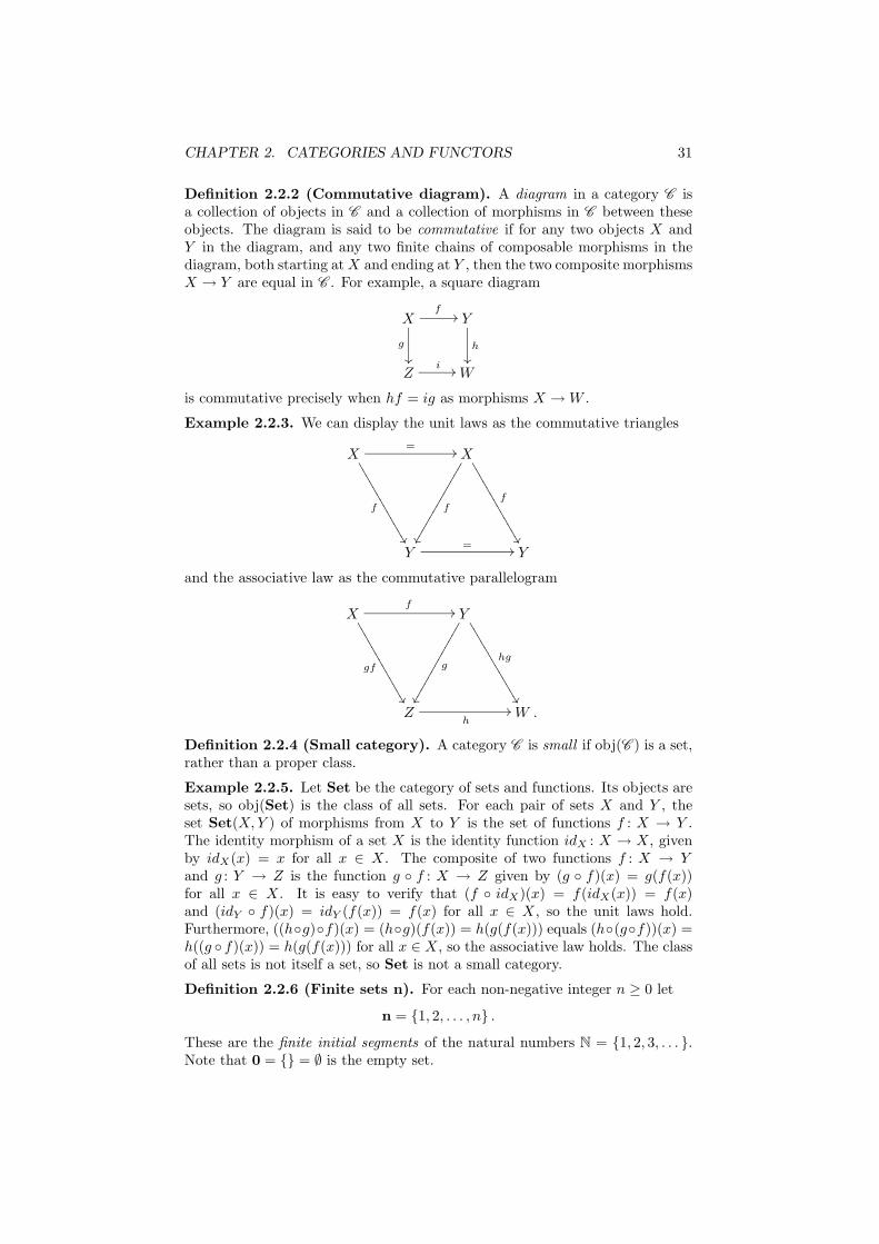
CHAPTER 2. CATEGORIES AND FUNCTORS 31
Definition 2.2.2 (Commutative diagram). A diagram in a category C isa collection of objects in C and a collection of morphisms in C between theseobjects. The diagram is said to be commutative if for any two objects X andY in the diagram, and any two finite chains of composable morphisms in thediagram, both starting at X and ending at Y , then the two composite morphismsX → Y are equal in C . For example, a square diagram
Xf
//
g
²²
Y
h
²²
Zi // W
is commutative precisely when hf = ig as morphisms X → W .
Example 2.2.3. We can display the unit laws as the commutative triangles
X= //
f
»»11
1111
1111
111 X
f
§§°°°°°°°°°°°°°
f
»»11
1111
1111
111
Y= // Y
and the associative law as the commutative parallelogram
Xf
//
gf
»»11
1111
1111
111 Y
g
§§°°°°°°°°°°°°°
hg
»»22
2222
2222
222
Zh
// W .
Definition 2.2.4 (Small category). A category C is small if obj(C ) is a set,rather than a proper class.
Example 2.2.5. Let Set be the category of sets and functions. Its objects aresets, so obj(Set) is the class of all sets. For each pair of sets X and Y , theset Set(X,Y ) of morphisms from X to Y is the set of functions f : X → Y .The identity morphism of a set X is the identity function idX : X → X, givenby idX(x) = x for all x ∈ X. The composite of two functions f : X → Yand g : Y → Z is the function g f : X → Z given by (g f)(x) = g(f(x))for all x ∈ X. It is easy to verify that (f idX)(x) = f(idX(x)) = f(x)and (idY f)(x) = idY (f(x)) = f(x) for all x ∈ X, so the unit laws hold.Furthermore, ((hg)f)(x) = (hg)(f(x)) = h(g(f(x))) equals (h(gf))(x) =h((g f)(x)) = h(g(f(x))) for all x ∈ X, so the associative law holds. The classof all sets is not itself a set, so Set is not a small category.
Definition 2.2.6 (Finite sets n). For each non-negative integer n ≥ 0 let
n = 1, 2, . . . , n .
These are the finite initial segments of the natural numbers N = 1, 2, 3, . . . .Note that 0 = = ∅ is the empty set.
CHAPTER 2. CATEGORIES AND FUNCTORS 32
Remark 2.2.7. The boldface may serve as a reminder that this is not the settheorists’ notation, since they usually define n to be the set 1, 2, . . . , n − 1.
Example 2.2.8. Let F be the skeleton category of finite sets. It is the categorywith objects the sets n for all n ≥ 0, and morphisms F (m,n) the set of functionsf : m → n, for each pair m, n ≥ 0. More explicitly, F (m,n) is the set offunctions
f : 1, 2, . . . ,m −→ 1, 2, . . . , n .
There are nm such functions. The identity functions and composition law in F
are defined in the same way as in Set, and the unit and associative laws holdby the same arguments as above. The class of objects in F is a set of subsetsof N, hence is itself a set, so F is a small category.
The term “skeleton category” will be explained in Definition 2.8.1, see alsoDefinition 3.2.11.
Definition 2.2.9 (Subcategory). A subcategory of a category D is a categoryC such that obj(C ) is a subclass of obj(D), and for each pair of objects X,Yin C the morphism set C (X,Y ) is a subset of the morphism set D(X,Y ).Furthermore, for each object X in C the identity morphism idX in C is thesame as the identity morphism in D , and for each pair of composable morphismsf and g in C , the composite g f in C is the same as their composite in D .
Definition 2.2.10 (Full subcategory). A subcategory C ⊆ D is said to befull if for each pair of objects X, Y in C the morphism set C (X,Y ) is equalto the morphism set D(X,Y ). A full subcategory C of D is thus determinedby its class of objects obj(C ), as a subclass of D . We say that C is the fullsubcategory generated by the subclass of objects obj(C ) in obj(D).
Example 2.2.11. The small category F of finite sets and functions is a fullsubcategory of the category Set of all sets and functions, namely the full sub-category generated by the objects n = 1, 2, . . . , n for n ≥ 0.
Example 2.2.12. Let Fin ⊂ Set be the full subcategory generated by all finitesets, not necessarily of the form n. This is not a small category, since the classof all finite sets is not itself a set.
Definition 2.2.13 (Opposite category). Given a category C , the oppositecategory C op has the same class of objects as C , but the morphisms in C op fromX to Y are the same as the morphisms in C from Y to X. Hence
obj(C op) = obj(C )
andC
op(X,Y ) = C (Y,X)
for all pairs X, Y of objects in C (or C op). For each object X, the identitymorphism of X in C op is equal to the identity morphism of X in C . For eachtriple X, Y , Z of objects the composition law
op : Cop(Y,Z) × C
op(X,Y ) −→ Cop(X,Z)
in C op is equal to the function
C (Z, Y ) × C (Y,X) −→ C (Z,X)
CHAPTER 2. CATEGORIES AND FUNCTORS 33
that takes a pair (g, f) of morphisms g : Z → Y and f : Y → X to their com-posite f g : Z → X in C , with f and g appearing in the opposite of the usualorder. Hence
g op f = f g .
With this notation it is straightforward to verify that C op is a category.
Lemma 2.2.14. (C op)op = C .
Proof. This is clear, since g (op)op f = f op g = g f .
Example 2.2.15. To describe the opposite Setop of the category of sets, wemust view a function f : X → Y as a morphism f in Setop(Y,X). One wayto encode the function f is in terms of the preimage sets f−1(y) = x ∈ X |f(x) = y for y ∈ Y . These are disjoint subsets of X that cover X. Hencea morphism Y → X in Setop can be defined to be a function F : Y → P(X)from Y to the power set P(X) of X, consisting of all subsets of X. We mustdemand that the values F (y) | y ∈ Y form a disjoint cover of X. The identitymorphism Y → Y is then the function I : Y → P(Y ) that takes y ∈ Y to thesingleton set y. Given another morphism Z → Y in Setop, represented by afunction G : Z → P(Y ) whose values form a disjoint cover of Y , the compositemorphism Z → X in Setop is represented by the function H : Z → P(X) givenby
H(z) =⋃
y∈G(z)
F (y)
for z ∈ Z. This reflects the formula (gf)−1(z) =⋃
y∈g−1(z) f−1(y).
Definition 2.2.16 (Product category). Given two categories C , C ′, theproduct category C × C ′ has as objects the pairs (X,X ′) where X is an objectin C and X ′ is an object in C ′:
obj(C × C′) = obj(C ) × obj(C ′) .
The morphisms in C × C ′ from (X,X ′) to (Y, Y ′) are the pairs (f, f ′) wheref : X → Y is a morphism in C and f ′ : X ′ → Y ′ is a morphism in C ′. Hence
(C × C′)((X,X ′), (Y, Y ′)) = C (X,Y ) × C
′(X ′, Y ′) .
Given a second morphism (g, g′) : (Y, Y ′) → (Z,Z ′), the composite in C ×C ′ isgiven by
(g, g′) (f, f ′) = (g f, g′ f ′) .
The identity morphism of (X,X ′) is (idX , idX′).
Definition 2.2.17. More generally, suppose given a category Ci for each ele-ment i in a set I. The product category
∏i∈I Ci has as objects families (Xi)i∈I
with Xi an object in Ci for each i ∈ I, and the morphisms from (Xi)i∈I to(Yi)i∈I are families (fi)i∈I of morphisms fi : Xi → Yi for all i ∈ I. Compositionis given by the formula
(gi)i∈I (fi)i∈I = (gi fi)i∈I .
The identity morphism of (Xi)i∈I is (idXi)i∈I .
CHAPTER 2. CATEGORIES AND FUNCTORS 34
When I = 1, 2 has two elements,∏
i∈I Ci can be identified with the prod-uct C1 × C2 defined above. When I = 1 has one element,
∏i∈I Ci can be
identified with the category C1. When I is empty, the product∏
i∈I Ci is thecategory ∗ with one object (an empty family of objects) and one morphism (anempty family of morphisms). We call ∗ the one-morphism category, since anyother category with precisely one morphism will also have precisely one object.
[[Later see that these are the products in the category of small categories,and that ∗ is the terminal object. Needs mention of the projection functorsprj :
∏i∈I Ci → Cj for all j ∈ I.]]
Definition 2.2.18 (Coproduct category). Given two categories C , C ′, thecoproduct category C ⊔ C ′ has object class the disjoint union
obj(C ⊔ C′) = obj(C ) ⊔ obj(C ′)
of the object classes of C and C ′, so an object of C ⊔C ′ is an object of C or ofC ′, and if C and C ′ have any objects in common, then we view them as beingdistinct in C ⊔ C ′. Given objects X, Y in C and X ′, Y ′ in C ′, all viewed asobjects in C ⊔ C ′, the morphisms in C ⊔ C ′ from X to Y are the same as themorphisms X → Y in C , the morphisms from X ′ to Y ′ are the same as themorphisms X ′ → Y ′ in C ′, and there are no morphisms X → Y ′ or X ′ → Y .In slightly different notation,
(C ⊔ C′)(X,Y ) =
C (X,Y ) if X,Y ∈ obj(C ),
C ′(X,Y ) if X,Y ∈ obj(C ′),
∅ otherwise.
Composition and identities are given as in C and C ′.The inclusions in : C → C ⊔ C ′ and in′ : C ′ → C ⊔ C ′ exhibit C and C ′ as
the full subcategories of C ⊔ C ′ generated by obj(C ) and obj(C ′), respectively.
Definition 2.2.19. More generally, suppose given a category Ci for each ele-ment i in a set I. The coproduct category
∐i∈I Ci has object class the disjoint
union of the object classes Ci. We may arrange that these object classes aredisjoint by labeling each object with the index in I:
obj(∐
i∈I
Ci) =⋃
i∈I
i × obj(Ci)
contained in I ×⋃
i∈I obj(Ci). This means that for each i ∈ I and X ∈ obj(Ci)we have an object (i,X) in
∐i∈I Ci, but we usually just write X for this object,
if i is clear from the context. Given two elements i, j ∈ I and objects X in Ci
and Y in Cj , there are no morphisms X → Y in∐
i∈I Ci unless i = j, in whichcase the morphisms are the same as in Ci. The inclusion inj : Cj →
∐i∈I Ci
exhibits Cj as the full subcategory of∐
i∈I Ci generated by obj(Cj), for eachj ∈ I.
When I = 1, 2 has two elements,∐
i∈I Ci can be identified with the co-product C1 ⊔C2 defined above. When I = 1 has one element,
∐i∈I Ci can be
identified with the category C1. When I is empty, the coproduct∐
i∈I Ci is theempty category ∅ with no objects and no morphisms.
[[Later see that these are the coproducts in the category of small categories,and that ∅ is the initial object.]]
CHAPTER 2. CATEGORIES AND FUNCTORS 35
2.3 Functors
There is a preferred way of comparing two categories, namely by a functor.Continuing the line of thought from the previous section, it follows that weshould view categories as the objects of a new category, whose morphisms arethe functors between these categories. More precisely, this turns out to workwell for functors between small categories.
Definition 2.3.1 (Functor). Let C and D be categories. A functor F : C → D
from C to D consists of two rules, one assigning to each object X of C an objectF (X) of D , and a second one assigning to each morphism f : X → Y in C amorphism F (f) : F (X) → F (Y ) in D . We can write the rule f 7→ F (f) as afunction
F : C (X,Y ) −→ D(F (X), F (Y ))
for each pair of objects X, Y in C . The rule on morphisms must satisfy
F (idX) = idF (X)
for each object X in C , and
F (g f) = F (g) F (f)
for each pair of composable morphisms f and g in C . Note that the compositeg f is formed in C , while the composite F (g) F (f) is formed in D .
The functor F maps each commutative triangle in C (as on the left)
Z F (Z)
 F //
Xf
//
gf
BB§§§§§§§§§§§§§§§Y
g
\\888888888888888
F (X)F (f)
//
F (gf)
BB§§§§§§§§§§§§§§F (Y )
F (g)
\\88888888888888
to a commutative triangle in D (as on the right). Hence F maps any commu-tative diagram in C to a commutative diagram in D of the same shape. Weoften simplify notation by writing f∗ for F (f), in which case the conditions offunctoriality appear as (idX)∗ = idF (X) and (gf)∗ = g∗f∗.
Example 2.3.2. Let F : F → Set be the functor that takes each object n in F ,for n ≥ 0, to the same set 1, 2, . . . , n, viewed as an object in Set. Furthermore,F takes each function f : m → n in F (m,n) to the same function, viewed asan element in Set(m,n). Since the identity morphisms and composition in F
was defined in the same way as in Set, it is clear that F is a functor.
Definition 2.3.3 (Full, faithful functor). A functor F : C → D is full iffor each pair of objects X, Y in C , the function C (X,Y ) → D(F (X), F (Y )) issurjective. The functor F is faithful if each function C (X,Y ) → D(F (X), F (Y ))is injective, for each pair X, Y of objects in C .
Example 2.3.4. Let C be a subcategory of D . The inclusion functor C → D ,given by the inclusions obj(C ) ⊆ obj(D) and C (X,Y ) ⊆ D(X,Y ) for all X,Y in C , is a faithful functor. It is full (and faithful) if and only if C is a fullsubcategory of D . For instance, the functor F : F → Set of Example 2.3.2 isthe full and faithful inclusion of F as a full subcategory of Set.
CHAPTER 2. CATEGORIES AND FUNCTORS 36
Definition 2.3.5 (Identity, composition of functors). For each category C
the inclusion functor of C into itself specifies the identity functor idC : C → C .Furthermore, given categories C , D , E and functors F : C → D and G : D → E
there is a composite functor G F : C → E , given by
(G F )(X) = G(F (X))
for each object X in C , and
(G F )(f) = G(F (f))
for each morphism f : X → Y in C . We often abbreviate G F to GF .It is easy to verify that idC and G F are functors. For example, given
another morphism g : Y → Z in C , we have G(F (g f)) = G(F (g) F (f)) =G(F (g)) G(F (f)), so (GF )(g f) = (GF )(g) (GF )(f).
Lemma 2.3.6. Let C and D be small categories. Then the collection of allfunctors F : C → D is a set.
Proof. Since obj(C ) and obj(D) are assumed to be sets, a functor consists ofa function F : obj(C ) → obj(D) and, for each pair of objects X,Y in C , afunction F : C (X,Y ) → D(F (X), F (Y )). There is a set of sets of sets of such,which is again a set. The collection of functors C → D is a subset of this set,hence is also a set.
Definition 2.3.7 (Category Cat). Let Cat be the category of small cate-gories. Its objects are the small categories C . The morphisms from C to D arethe functors F : C → D . By the lemma above, the collection Cat(C ,D) of allsuch functors is a set, since C is small. The identity functor, and compositionof functors, define the identities and composition in Cat.
Definition 2.3.8 (Contravariant functor). A contravariant functor F fromC to D is the same as a functor F : C op → D from the opposite category of C toD . It thus consists of two rules, one assigning to each object X of C an objectF (X) of D , and another assigning to each morphism f : X → Y in C , which isthe same as a morphism f : Y → X in C op, a morphism F (f) : F (Y ) → F (X)in D . (Note how the direction of the morphism F (f) is reversed, compared toDefinition 2.3.1.) We can write the rule f 7→ F (f) as a function
F : C (X,Y ) −→ D(F (Y ), F (X))
for each pair of objects X, Y in C . The rule on morphisms satisfies
F (idX) = idF (X)
for each object X in C , and
F (g f) = F (f) F (g)
for each pair of composable morphisms f and g in C .We often simplify notation by writing f∗ for F (f), so that the conditions
for contravariant functoriality become (idX)∗ = idF (X) and (gf)∗ = f∗g∗.
CHAPTER 2. CATEGORIES AND FUNCTORS 37
Remark 2.3.9. A functor as in Definition 2.3.1 is sometimes called a covariantfunctor, to distinguish it from contravariant functors. Sometimes it is moreconvenient to view a contravariant functor F from C to D as a functor F : C →Dop. The rules and conditions are the same. We may even consider a covariantfunctor from C to D as a functor F op : C op → Dop. This can be useful whenconsidering a composite of covariant and contravariant functors.
Definition 2.3.10 (Corepresented functors). Fix an object X in a categoryC . We define a (covariant) functor
YX : C −→ Set
by taking each object Y in C to the set Y X(Y ) = C (X,Y ) of morphismsf : X → Y in C , from the fixed object X, and taking each morphism g : Y → Zin C to the function
g∗ = YX(g) : Y
X(Y ) = C (X,Y ) −→ C (X,Z) = YX(Z)
that maps f : X → Y to the composite gf : X → Z.
Xf
~~~~~~
~~~
gf
ÃÃ@@
@@@@
@
Yg
// Z
We call Y X the set-valued functor corepresented by X in C . It may also bedenoted Y X(−) = C (X,−).
Definition 2.3.11 (Represented functors). Fix an object Z in a categoryC . We define a contravariant functor
YZ : Cop −→ Set
by taking each object Y in C to the set YZ(Y ) = C (Y,Z) of morphisms g : Y →Z in C , to the fixed object Z, and taking each morphism f : X → Y in C tothe function
f∗ : YZ(f) : YZ(Y ) = C (Y,Z) −→ C (X,Z) = YZ(X)
that maps g : Y → Z to the composite gf : X → Z.
Y
gÂÂ
@@@@
@@@ X
foo
gf~~~~
~~~~
~
Z
We call YZ the contravariant set-valued functor represented by Z in C . It mayalso be denoted YZ(−) = C (−, Z).
Remark 2.3.12. Functors of the form Y X and YZ are called corepresentableand representable, respectively. The contravariant functor YZ represented by Zin C is the same as the covariant functor Y Z corepresented by Z in the oppositecategory, C op. [[Forward reference to Yoneda embedding and Yoneda’s lemma.]][[Example: The n-simplex ∆n is the representable functor ∆(−, [n]) : ∆op →Set.]]
CHAPTER 2. CATEGORIES AND FUNCTORS 38
Definition 2.3.13 (Bifunctor). A bifunctor F from C and C ′ to D is thesame as a functor F : C × C ′ → D from the product category of C and C ′ toD . It associates to each pair of objects (X,X ′), with X in C and X ′ in C ′, anobject F (X,X ′) in D , and to each pair of morphisms (f, f ′), with f : X → Yin C and f ′ : X ′ → Y ′ in C ′, a morphism F (f, f ′) : F (X,X ′) → F (Y, Y ′) in D .We can write the rule (f, f ′) 7→ F (f, f ′) as a function
F : C (X,Y ) × C′(X ′, Y ′) −→ D(F (X,X ′), F (Y, Y ′)) .
It satisfiesF (idX , idX′) = idF (X,X′)
for each object X in C and each object X ′ in C ′, and
F (g f, g′ f ′) = F (g, g′) F (f, f ′)
for each composable pair f and g in C and each composable pair f ′ and g′ in C ′.In view of the relation
(f, idY ′) (idX , f ′) = (f, f ′) = (idY , f ′) (f, idX′)
in C × C ′ it suffices to specify the rule on morphisms in the cases F (f, idX′)and F (idX , f ′), for all morphisms f : X → Y in C , f ′ : X ′ → Y ′ in C ′ and allobjects X in C and X ′ in C ′, subject to the condition
F (f, idY ′) F (idX , f ′) = F (idX , f ′) F (f, idX′) .
[[Proof?]]
Example 2.3.14. Let C be any category. We define a bifunctor
C (−,−) : Cop × C → Set
by taking each object (X,X ′) in C op × C to the set of morphisms C (X,X ′)in C . A morphism (f, f ′) : (X,X ′) → (Y, Y ′) in C op × C consists of a pair ofmorphisms f : Y → X and f ′ : X ′ → Y ′ in C . The rule
f ′∗f
∗ = f∗f ′∗ = C (f, f ′) : C (X,X ′) → C (Y, Y ′)
maps g : X → X ′ to the composite f ′ g f : Y → Y ′.
X
g
²²
Yf
oo
f ′gf
²²
X ′f ′
// Y ′
In other words, the morphisms sets in a category define a bifunctor to Set,contravariant in the first factor (the source) and covariant in the second factor(the target).
Remark 2.3.15. A functor C ⊔ C ′ → D is more-or-less the same as a pairof functors C → D and C ′ → D . Likewise, a functor C → D × D ′ can beidentified with a pair of functors C → D and C → D ′. We do not introducespecial terminology for these cases. Functors C → D ⊔D ′ might call for specialterminology, but are rarely needed.
CHAPTER 2. CATEGORIES AND FUNCTORS 39
Definition 2.3.16 (Diagonal and fold functors). Let C be any category.The diagonal functor
∆: C −→∏
i∈I
C
takes X to the family ∆(X) = (Xi)i∈I with each Xi = X, and f : X → Y tothe family ∆(f) = (fi)i∈I with each fi = f . The fold functor
∇ :∐
i∈I
C −→ C
takes (i,X) to X and (i, f) : (i,X) → (i, Y ) to f : X → Y , for each i ∈ I.
2.4 Isomorphisms and groupoids
Definition 2.4.1 (Isomorphism). Let f : X → Y be a morphism in a categoryC . If g : Y → X satisfies g f = idX we say that g is a left inverse to f . Ifg satisfies f g = idY we say that g is a right inverse to f . If g satisfies bothg f = idX and f g = idY , then we say that f : X → Y is an isomorphismin C , or that f is invertible, and we call g : Y → X an inverse to f . We often
write f : X∼=−→ Y to indicate that f is an isomorphism. If such an isomorphism
f exists we say that X and Y are isomorphic in C , and write X ∼= Y .
Lemma 2.4.2. If f : X → Y has a left inverse g : Y → X and a right inverseh : Y → X, then g = h and f is an isomorphism. Hence an isomorphismf : X → Y has a unique inverse, which we can denote by f−1 : Y → X.
Proof. If gf = idX and f h = idY then g = g idY = g(f h) = (gf)h =idX h = h. Hence g = h is both a left and a right inverse to f , so f isinvertible.
Lemma 2.4.3. Each identity morphism in a category is its own inverse, id−1X =
idX , and the composite gf of two composable isomorphisms f : X → Y andg : Y → Z is an isomorphism, with inverse (gf)−1 = f−1g−1. The inverse f−1
of an isomorphism f : X → Y is an isomorphism, with inverse (f−1)−1 = f .
Proof. It is clear that idX idX = idX , so idX is its own inverse. To see thatf−1g−1 is an inverse to gf , we compute f−1g−1(gf) = f−1 idY f = f−1f =idX and (gf)f−1g−1 = g idY g−1 = gg−1 = idZ . The relations f−1f = idX
and ff−1 = idY exhibiting f−1 as an inverse to f also exhibit f as the inverseto f−1.
Lemma 2.4.4. Let f : X → Y and g, h : Y → X be morphisms in C . Ifgf : X → X is an isomorphism, then (gf)−1 g : Y → X is a left inverse to f .If fh : Y → Y is an isomorphism, then h (fh)−1 : Y → X is a right inverse tof . Hence if gf and fh are isomorphisms, then f is invertible.
Proof. (gf)−1gf = (gf)−1(gf) = idX and f h(fh)−1 = (fh)(fh)−1 = idY ,so this is clear.
Example 2.4.5. Let f : X → Y be a morphism in Set, that is, a function.Then f admits a left inverse in Set if and only if f is injective (= one-to-one),
CHAPTER 2. CATEGORIES AND FUNCTORS 40
and f admits a right inverse if and only if f is surjective (= onto). In mostcases, these left and right inverses are not unique. A function f : X → Y is anisomorphism if and only if it is bijective (= one-to-one and onto).
Example 2.4.6. A morphism f : m → n in F is an isomorphism if and only ifit is a bijection. This can only happen if m = n, as can be proved by inductionon n. A bijection
f : 1, 2, . . . , n∼=−→ 1, 2, . . . , n
is also known as a permutation of the set n = 1, 2, . . . , n. There are n!such permutations. Let Σn be the symmetric group of such permutations, withgroup operation given by composition and neutral element given by the identitypermutation. In the language of Definition 2.8.11, Σn is the automorphismgroup of n in F .
Exercise 2.4.7. How many injective functions f : m → n are there? Howmany surjective functions f : m → n are there? (The first is easy, the secondinvolves Stirling numbers of the second kind. Later, we shall be interested in thecorresponding questions for order-preserving functions.) [[Forward reference.]]
Definition 2.4.8 (Isomorphic categories). We say that two categories C
and D are isomorphic if there exist functors F : C → D and G : D → C suchthat G F = idC and F G = idD . We then say that F : C → D is anisomorphism of categories, and G : D → C is the inverse isomorphism. If C
and D are small, this is the same as saying that C and D are isomorphic asobjects in the category Cat of small categories. Both functors F and G arethen full and faithful, and on objects they induce a bijection between obj(C )and obj(D).
Definition 2.4.9 (Groupoid). A groupoid is a category in which each mor-phism is an isomorphism. We write Gpd for the category of small groupoidsand functors. It is the full subcategory of Cat generated by the small categoriesthat are groupoids. Hence there is an inclusion functor Gpd ⊂ Cat.
Definition 2.4.10 (Interior groupoid). Given a category C , let iso(C ) ⊆C be the subcategory with the same objects as C , and with morphism setiso(C )(X,Y ) the subset of C (X,Y ) consisting of the morphisms f : X → Ythat are isomorphisms in C . Identity morphisms exist and composition is well-defined in iso(C ), by Lemma 2.4.3. The unit laws and associative law in iso(C )are inherited from those in C . Since the inverse of an isomorphism in C is anisomorphism in C , each morphism in iso(C ) has an inverse in iso(C ), so iso(C )is a groupoid.
Exercise 2.4.11. Let C be a category such that each morphism has a leftinverse. Show that C is a groupoid. Similarly if each morphism has a rightinverse.
Definition 2.4.12 (π0 of groupoid). When C is small, Lemma 2.4.3 showsthat isomorphism of objects is an equivalence relation on obj(C ). We write
π0(iso(C )) = obj(C )/ ∼=
for the set of isomorphism classes of objects in C , and denote the isomorphismclass of an object X by
[X] = Y ∈ obj(C ) | X ∼= Y .
CHAPTER 2. CATEGORIES AND FUNCTORS 41
Example 2.4.13. By Example 2.4.5, iso(Set) is the groupoid of sets and bijec-tive functions. By Example 2.4.6, the groupoid iso(F ) has objects n for n ≥ 0,the morphism set iso(F )(m,n) is empty for m 6= n, and iso(F )(n,n) = Σn forall n ≥ 0. In particular, iso(F ) is the full subcategory of iso(Set) generated bythe objects n for n ≥ 0.
Lemma 2.4.14. iso(C op) = (isoC )op.
Proof. This is clear, since the opposite gop of a left inverse g of f is a rightinverse of fop, and similarly with left and right exchanged.
Lemma 2.4.15. iso(C ×C ′) = iso(C )× iso(C ′), iso(C ⊔C ′) = iso(C )⊔ iso(C ′)and similarly for arbitrary set-indexed products and coproducts.
Proof. A family (gi)i∈I is inverse in∏
i∈I Ci to a given family (fi)i∈I if andonly if gi is inverse to fi for each i ∈ I. This proves the case of products. Amorphisms fj in Cj is invertible in Cj if and only if it is invertible in
∐i∈I Ci.
This proves the case of coproducts.
Lemma 2.4.16. Let F : C → D be a functor. If f : X∼=−→ Y is an isomorphism
in C , then F (f) : F (X)∼=−→ F (Y ) is an isomorphism in D .
Proof. Let g : Y → X be the inverse to f . Then F (g) is inverse to F (f), sinceF (g) F (f) = F (g f) = F (idX) = idF (X) and F (f) F (g) = F (f g) =F (idY ) = idF (Y ).
Lemma 2.4.17. Any functor F : D → C from a groupoid D factors uniquelythrough the inclusion ǫ : iso(C ) ⊆ C , so iso(C ) is the maximal subgroupoid ofC .
Proof. For each object X in D , F (X) is an object of C , hence also an objectof iso(C ). Each morphism f : X → Y in D is an isomorphism, since D isassumed to be a groupoid, so F (f) is an isomorphism in C by Lemma 2.4.16,hence a morphism in iso(C ). Hence F factors in a unique way as a compositeD → iso(C ) ⊆ C .
Lemma 2.4.18. The rule iso that takes a small category C to its maximalsubgroupoid iso(C ) defines a functor
iso : Cat −→ Gpd .
The composite functor Gpd ⊂ Catiso−→ Gpd equals the identity.
Proof. We must explain how each functor F : C → D , which is a morphism
in Cat, induces a functor iso(F ) : iso(C ) → iso(D). Each morphism f : X∼=−→
Y in iso(C ) is an isomorphism in C , hence maps to an isomorphism F (f) in D ,by Lemma 2.4.16. Hence F (f) is a morphism in iso(D), which we define to beiso(F )(f). It is immediate that iso(F ) becomes a functor. The last claim isclear.
Instead of restricting attention to the morphisms in C that are already iso-morphisms, one may extend C so as to make all morphisms into isomorphisms,at least if C is small.
CHAPTER 2. CATEGORIES AND FUNCTORS 42
Definition 2.4.19 (Localized groupoid). Given a small category C , letC [C−1] be the groupoid with the same objects as C , and with morphisms fromX to Y in C [C−1] the equivalence classes of chains (f ǫm
m , . . . , f ǫ11 ) of morphisms
in C ,
X = Z0oo
f±11 // Z1
oof±12 // . . . oo
f±1m−1
// Zm−1oo
f±1m // Zm = Y
where m ≥ 1 and each ǫi ∈ ±1, that are composable in the sense that thereare objects Z0, . . . , Zm in C , with Z0 = X, Zm = Y , fi ∈ C (Zi−1, Zi) if ǫi = +1and fi ∈ C (Zi, Zi−1) if ǫi = −1, subject to the equivalence relation generatedby the rules
(g+1, f+1) ∼ ((gf)+1) (f−1, g−1) ∼ ((gf)−1)
(f+1, f−1) ∼ (id+1) (f−1, f+1) ∼ (id+1) ,
in the sense that (a, x, b) ∼ (a, y, b) for possibly empty words a and b, wheneverx ∼ y.
Composition in C [C−1] is given by concatenation. The identity morphismof X is (id+1
X ), and the inverse of (f ǫmm , . . . , f ǫ1
1 ) is (f−ǫm
1 , . . . , f−ǫ1m ). There is a
functorη : C → C [C−1] ,
which is the identity on objects and takes f : X → Y to (f+1). We call C [C−1]the localization of C with respect to all morphisms.
Remark 2.4.20. If C is not small, there may be a proper class of diagramsX ← Z → Y in C , even if X and Y are fixed in advance. Hence the constructionabove may not provide a (small) set of morphisms from X to Y in C [C−1]. IfC is small, there is only a set of morphisms in C , hence only a set of words(f ǫm
m , . . . , f ǫ11 ), so C [C−1] becomes an honest category.
Lemma 2.4.21. Any functor F : C → D from a small category C to a groupoidD extends uniquely over η : C → C [C−1], so C [C−1] is the initial groupoidunder C .
Proof. The extension must map (f ǫmm , . . . , f ǫ1
1 ) in C [C−1] to the composite
F (fm)ǫm · · · F (f1)ǫ1
in D , and this is well-defined.
Lemma 2.4.22. The rule L that takes a small category C to the localizationL(C ) = C [C−1] defines a functor
L : Cat −→ Gpd .
The composite functor Gpd ⊂ CatL
−→ Gpd is the identity.
Proof. We must explain how each functor F : C → D induces a functor
L(F ) : C [C−1] → D [D−1] .
On objects, L(F ) takes X to F (X). On morphisms, L(F ) takes (f ǫmm , . . . , f ǫ1
1 )in C [C−1] to (F (fm)ǫm , . . . , F (f1)
ǫ1) in D [D−1].
CHAPTER 2. CATEGORIES AND FUNCTORS 43
2.5 Ubiquity
Practically all sorts of mathematical objects naturally occur as the objects of acategory. Here are some common examples.
Definition 2.5.1 (Groups). Let Grp be the category of groups and grouphomomorphisms. Its object class obj(Grp) is the proper class of all groups. Wewrite general groups multiplicatively, with neutral element e. For each pair ofgroups G, H, the morphism set Grp(G,H) is the set of group homomorphismsf : G → H, i.e., the functions f : G → H such that f(xy) = f(x)f(y) for all x,y ∈ G. It follows formally that f(e) = e and f(x−1) = f(x)−1. The identityfunction idG : G → G is a group homomorphism, and the composite of twogroup homomorphisms f : G → H and g : H → K is a group homomorphismgf : G → K, since (gf)(xy) = g(f(xy)) = g(f(x)f(y)) = g(f(x))g(f(y)) =(gf)(x)(gf)(y). The unit and associative laws hold as in Set, so Grp is acategory. An isomorphism of groups has the usual meaning.
Definition 2.5.2 (Abelian groups). Let Ab be the category of abelian groupsand group homomorphisms. This is the full subcategory of Grp generatedby the proper class of all abelian groups. We usually write abelian groupsadditively, with neutral element 0. For each pair of abelian groups A, B, themorphism set Ab(A,B) is the set of group homomorphisms f : A → B, i.e., thefunctions f : A → B such that f(x+y) = f(x)+f(y) for all x, y ∈ A. It followsformally that f(0) = 0 and f(−x) = −f(x). An isomorphism of abelian groupshas the usual meaning.
Remark 2.5.3. In this case, the morphism set Ab(A,B) = Hom(A,B) is well-known to have the additional structure of an abelian group. For example, thesum f + g of two group homomorphisms f , g : A → B is given by the formula(f + g)(x) = f(x) + g(x) for all x ∈ A. However, this abelian group structure isnot part of the data when we say that Ab is a category. Categories with thiskind of additional structure are called additive categories, or Ab-categories.[[Reference to the chapter on abelian and exact categories.]]
Example 2.5.4. Let Z/n be the cyclic group of order n. For each abelian groupB, the abelian group Hom(Z/n,B) of group homomorphisms f : Z/n → B canbe identified with the subgroup B[n] = x ∈ B | nx = 0 of elements of orderdividing n in B. The rule B 7→ B[n] defines a covariant functor Ab → Ab,which is corepresented by the object Z/n in Ab, viewed as an additive category.
Example 2.5.5. Let T = U(1) be the multiplicative group of complex numbersof absolute value 1. For each group A, the abelian group A# = Hom(A, T) ofgroup homomorphisms f : A → T is called the character group, or the Pontrya-gin dual of A. The rule A 7→ A# defines a contravariant functor Abop → Ab,which is represented by the object T in Ab, viewed as an additive category.There is a natural homomorphism A → (A#)#, which is an isomorphism forall finite groups A. [[Better to discuss Pontryagin duality theorem in the addi-tive topological setting, between discrete abelian groups and compact Hausdorffabelian groups.]]
Definition 2.5.6 (Abelianization). Given a group G, the commutator sub-group [G,G] ⊆ G is the subgroup generated by the set of commutators [g, h] =
CHAPTER 2. CATEGORIES AND FUNCTORS 44
ghg−1h−1 ∈ G, for all g, h ∈ G. In other words, the elements of [G,G] areall finite products of commutators in G. This is a normal subgroup, sincek[g, h]k−1 = [kgk−1, khk−1] is a commutator for all k ∈ G. The quotient group
Gab = G/[G,G]
is called the abelianization of G. It is an abelian group, since [g][h][g]−1[h]−1 =[ghg−1h−1] = e is the neutral element in Gab for any g, h ∈ G, which implies[g][h] = [h][g]. Here [g] denotes the coset of g, which is the image of g ∈ G underthe canonical homomorphism G → Gab. Any group homomorphism f : G → Ato an abelian group A factors uniquely through this canonical homomorphism,since f([g, h]) = 0 for any commutator.
Lemma 2.5.7. The rule taking G to Gab defines a functor
(−)ab : Grp −→ Ab .
The composite functor Ab ⊂ Grp(−)gp
−→ Ab is the identity.
[[Discuss as adjunction later. Abelianization is left adjoint to the full embed-ding. The isomorphism Hgp
1 (G) ∼= Gab is generalized by Quillen [53], defininghomology as left derived functors of abelianization, where abelianization is leftadjoint to a forgetful functor from abelian group objects. The full embeddingdoes not respect coproducts, hence has no right adjoint.]]
Proof. A homomorphism f : G → H takes [G,G] into [H,H], since f([g, h]) =[f(g), f(h)], hence induces a homomorphism fab : Gab → Hab. Functorialityis easily verified. If G is already abelian, [G,G] = e and we will identifyGab = G/e with G.
Remark 2.5.8. For a related example of something that is not a functor,consider the rule taking a group G to its center
Z(G) = g ∈ G | gh = hg for all h ∈ G .
This is a well-defined abelian group, and the group inclusion Z(G) ⊆ G is suchthat every group homomorphism A → G from an abelian group factors uniquelythrough Z(G). Still, Z is not a functor, since for a group homomorphism f : G →H there is not necessarily an induced homomorphism Z(f) : Z(G) → Z(H). Forexample, with G = Σ2, H = Σ3 and f : Σ2 → Σ3 the usual inclusion, Z(G) = Gwhile Z(H) ∼= Z/3 is generated by the cyclic permutation (123). Since f admitsa left inverse the induced homomorphism Z(f) : Z(G) → Z(H) should alsoadmit a left inverse. But the only homomorphism Z(G) → Z(H) is the trivialone.
Example 2.5.9. For a group G, the set of homomorphisms G# = Grp(G, T)forms an abelian group, under pointwise multiplication. Since any commutatorin G must map to 1 under such a homomorphism, the projection G → Gab
induces an isomorphism (Gab)# ∼= G#. Hence, for each finite group G, (G#)# ∼=Gab. To study non-abelian groups G, one can instead consider the category ofunitary G-representations, or equivalently, the group homomorphisms ρ : G →U(n) for varying n ≥ 1, and then attempt to recover G from that category. SeeSection 3.3 for more about this.
CHAPTER 2. CATEGORIES AND FUNCTORS 45
Example 2.5.10. Let Top be the category of topological spaces and continuousfunctions. The morphism set Top(X,Y ) between two topological spaces X andY is the set of continuous functions f : X → Y . Recall that a function f : X → Yis continuous if f−1(U) = x ∈ X | f(x) ∈ U is open in X for each opensubset U ⊆ Y . Continuous functions are usually called maps, and the elementsx ∈ X in a topological space are usually called points. The identity functionidX is continuous, and the composite of two continuous functions f : X → Yand g : Y → Z is continuous, since g−1(V ) is open in Y , and (gf)−1(V ) =f−1(g−1(V )) is open in X, for each open subset V ⊆ Z. The unit and associativelaws hold as in Set, so Top is a category.
Remark 2.5.11. We might identify Set with the full subcategory of Top gen-erated by the discrete topological spaces, since any function f : X → Y is con-tinuous when X (and Y ) is given the discrete topology. In the language ofDefinition 2.4.8, Set is isomorphic to this full subcategory. For general topolog-ical spaces X and Y we might give the set Top(X,Y ) = Map(X,Y ) a topology,for instance the compact–open topology. Under mild assumptions on Y , like lo-cal compactness, the composition Top(Y,Z)×Top(X,Y ) → Top(X,Z) is thena continuous map, and we obtain a topological category. Since some assumptionsare needed, we postpone the details to a later section. [[Forward reference.]]
Example 2.5.12. Let S1 be the circle. Given any space X the continuousmaps f : S1 → X are called free loops in X. When the set Top(S1,X) offree loops is given the compact–open topology, we call it the free loop spaceL X = Map(S1,X) of X. It can, for instance, be considered as the space ofclosed strings in X.
Definition 2.5.13 (Path components). Let I = [0, 1] ⊂ R be the unitinterval on the real line, and let X be any topological space. A map α : I → Xis called a path in X, from α(0) to α(1). We say that two points x, y ∈ X are inthe same path component of X, and write x ≃ y, if there exists a path α in Xfrom x to y. This defines an equivalence relation on the set of points in X, aswe will verify in a moment. The set of equivalence classes for this relation willbe called the set of path components of X, and is denoted
π0(X) = X/≃ .
It remains to verify that ≃ is an equivalence relation on X. The constant pathα(s) = x for all s ∈ I shows that x ≃ x. If α is a path from x to y, so thatx ≃ y, then there is a path α from y to x given by the formula α(s) = α(1 − s)for all s ∈ I, so that y ≃ x. If α is a path from x to y, and β is a path from yto z, so that x ≃ y and y ≃ z, then there is a path α ∗ β from x to z, given by
(α ∗ β)(s) =
α(2s) for 0 ≤ s ≤ 1/2,
β(2s − 1) for 1/2 ≤ s ≤ 1,
so that x ≃ z. [[Should we write α ∗ β or β ∗ α for this?]]
Lemma 2.5.14. The rule taking X to π0(X) defines a functor
π0 : Top −→ Set .
The composite functor Set ⊂ Topπ0−→ Set is the identity.
CHAPTER 2. CATEGORIES AND FUNCTORS 46
[[Mention later that π0 is left adjoint to the inclusion for reasonable (locallypath-connected) X.]]
Proof. A continuous map f : X → Y takes each path component of X into apath component of Y , since if α : I → X is a path from x to y in X, so thatx ≃ y, then the composite f α : I → Y is a path from f(x) to f(y) in Y , sothat f(x) ≃ f(y). Hence
π0(f) : π0(X) −→ π0(Y )
is well-defined by taking [x] to [f(x)], where [x] ∈ π0(X) denotes the equivalenceclass (= path component) of x under ≃. Functoriality is easily verified.
2.6 Correspondences
Example 2.6.1. Given two sets X, Y , a correspondence C from X to Y is asubset C ⊆ X × Y . We can think of C as a multi-valued function from X toY , whose values at x ∈ X is the set of y ∈ Y such that (x, y) ∈ C. Let Corbe the category of sets and correspondences. Its objects are sets, so obj(Cor)is the class of all sets. For each pair of sets X, Y , Cor(X,Y ) is the set ofcorrespondences from X to Y , i.e., the set of all subsets of X ×Y . The identitycorrespondence from X to X is the diagonal subset ∆(X) = (x, x) | x ∈ X ofX×X. Given sets X, Y , Z and correspondences C ⊆ X×Y and D ⊆ Y ×Z, wedefine the composite correspondence D C ⊆ X ×Z as the set of (x, z) ∈ X ×Zsuch that there exists at least one y ∈ Y with (x, y) ∈ C and (y, z) ∈ D. Theunit and associative laws are easy to verify, so Cor is a category.
Remark 2.6.2. The last example shows that the morphisms in a categorydo not need to have preferred underlying functions. Similarly, there is no re-quirement that the objects of a category have preferred underlying sets. Thisexample is also a little unusual in that we have chosen to label the category Corby the name for its morphisms, rather than its objects. In many cases it is clearwhat the intended morphisms are once the objects are described, in which caseit makes sense to refer to the category primarily by its objects. In other cases,where it is the morphisms that are unobvious, it seems sensible to emphasizethem in the notation.
[[Define a concrete category.]]
Example 2.6.3. The opposite Corop of the category of correspondences canbe identified with Cor itself, so this category is self-dual. The identification isthe identity on objects, and for sets X, Y we identify Cor(X,Y ) with
Corop(X,Y ) = Cor(Y,X)
by taking a correspondence C ⊆ X × Y to the correspondence γC ⊆ Y × X,where
γC = (y, x) ∈ Y × X | (x, y) ∈ C .
More precisely, this defines an isomorphism of categories γ : Cor ∼= Corop, inthe sense of Definition 2.4.8, since for D ⊆ Y ×Z the composite D C ⊆ X ×Zin Cor corresponds to γ(D C) = γD op γC in Corop.
CHAPTER 2. CATEGORIES AND FUNCTORS 47
Example 2.6.4. Let G : Set → Cor be the functor that is the identity onobjects, so that G(X) = X for all sets X, and takes each function f : X → Yto its graph
G(f) = (x, f(x)) | x ∈ X ⊆ X × Y
considered as a correspondence from X to Y . The rule f 7→ G(f) defines afunction Set(X,Y ) → Cor(X,Y ) for all sets X, Y . The graph of the identityfunction idX : X → X is the diagonal subset G(idX) = ∆(X) ⊆ X × X, soG takes identities to identities. For G to be a functor, we must also checkthat G takes composites in Set to composites in Cor. Thus consider functionsf : X → Y and g : Y → Z. The composite correspondence G(g) G(f) consistsof the (x, z) ∈ X × Z such that there exists a y ∈ Y with (x, y) ∈ G(f) and(y, z) ∈ G(g). Since G(f) is the graph of the function f , the only y satisfyingthe first condition is y = f(x). Then the only z satisfying the second conditionis z = g(y) = (g f)(x). Hence
G(g) G(f) = (x, z) | z = (g f)(x) = G(g f) ,
and G is, indeed, a functor.
Example 2.6.5. The functor G : Set → Cor is faithful, since for every pair X,Y of sets the function
G : Set(X,Y ) −→ Cor(X,Y )
is injective. A function f : X → Y is after all determined by its graph. For mostpairs X, Y there are more correspondences than functions between X and Y ,so G is not full.
Example 2.6.6. Let C ⊂ Cor be the subcategory of correspondences with allsets as objects, but with morphisms C (X,Y ) only the correspondences C ⊆X ×Y that are graphs of functions, i.e., those having the property that for eachx ∈ X there is one and only one y ∈ Y with (x, y) ∈ C. The graph functorfrom Example 2.6.4 factors uniquely through C , and induces an isomorphism
of categories Set∼=−→ C .
Remark 2.6.7. This example presumes that we think of a function f : X → Yas a rule that associates to each element x ∈ X a unique element f(x) in Y ,and that this is not exactly the same as the graph subset G(f) ⊆ X × Y . If the
reader prefers to define functions as graphs, then the isomorphism Set∼=−→ C
is an equality, and Set is a subcategory of Cor.
2.7 Representations of groups and rings
Definition 2.7.1 (G-sets). Let G be a group with neutral element e. A (left)G-set is a set X with a left action map
G × X −→ X
taking (g, x) to g · x, such that e · x = x and g · (h · x) = gh · x for all g, h ∈ G,x ∈ X. We often abbreviate g · x to gx. A function f : X → Y between two leftG-sets is said to be G-equivariant if gf(x) = f(gx) for all g ∈ G, x ∈ X.
CHAPTER 2. CATEGORIES AND FUNCTORS 48
Definition 2.7.2 (Category G−Set). Let G−Set be the category of all (left)G-sets and G-equivariant functions. Each identity function is G-equivariant, andthe composite of two G-equivariant functions is G-equivariant, so this defines acategory. Let G−Fin be the full subcategory of G−Set generated by all finiteG-sets, i.e., G-sets X such that X is a finite set.
Definition 2.7.3 (Orbits and fixed points). Let X be a G-set, and letx ∈ X. The orbit of x is the G-subset
Gx = gx ∈ X | g ∈ G
of X, and the stabilizer group of x is the subgroup
Gx = g ∈ G | gx = x
of X. We say that the G-action on X is transitive if Gx = X for some (henceall) x ∈ X. We say that the G-action is free if gx = x only for g = e, so thatthe stabilizer group Gx = e is trivial for each x ∈ X. The G-action is trivialif gx = x for all g ∈ G and x ∈ X, so each stabilizer group Gx = G equals thewhole group. The orbit set X/G = Gx | x ∈ X is the set of orbits, and thefixed point set XG = x ∈ X | Gx = G is the set of x with gx = x for all g.
Lemma 2.7.4. Any G-set X decomposes as the disjoint sum of its orbits
X ∼=∐
x
Gx
where x ranges over one element in each orbit. Each orbit is a transitive G-set,and there is an isomorphism
G/Gx
∼=−→ Gx
of G-sets taking the coset gGx to the element gx. Each G-set is therefore of theform
X ∼=∐
i∈I
G/Hi
where Hi is a subgroup of G for each i ∈ I.
Lemma 2.7.5. The G-equivariant functions f : G/H → G/K can be uniquelywritten in the form f(gH) = gwK for an element wK ∈ (G/K)H , [[Make(G/K)H explicit.]] Each G-equivariant function
f :∐
i∈I
G/Hi −→∐
j∈J
G/Kj
has the formf(gHi) = gwiKφ(i)
for a unique function φ : I → J and uniquely determined family of elementswiKj ∈ (G/Kj)
Hi , with j = φ(i).
[[Discuss orbit category Or(G) of transitive G-sets G/H for H ⊆ G, as afull subcategory of G−Set.]]
CHAPTER 2. CATEGORIES AND FUNCTORS 49
[[Discuss the isomorphism classes of G−Set or G−Fin. Decompose G-setsinto orbits G/H, classified by the conjugacy class (H) of H in G. Form a skeletoncategory G−F with objects
∐(H)
∐nH G/H for some (class) function n fromconjugacy classes of subgroups to N0. Give criterion for finiteness. Specializeto G finite. Alternatively, consider group homomorphisms G → Σn, whichcorrespond to G-actions on n. These are permutation representations of G.Conjugate group homomorphisms give isomorphic G-sets.]]
[[Categories of left and right R-modules, R−Mod and Mod−R, for R aring. The full subcategory R−Coh of coherent = finitely generated R-modulesfor R left Noetherian, or the full subcategory R−Proj of finitely generatedprojective R-modules.]]
[[Exactness of HomR(−,−), projective and injective R-modules. Exactnessof (−) ⊗R (−), left and right flat R-modules.]]
[[Discuss the isomorphism classes of R−Mod or its various full subcate-gories.]]
[[Example: Let R be a commutative ring. Define D : (R − Mod)op → R −Mod by D(M) = (R − Mod)(M,R).]]
2.8 Few objects
To get more easily comprehended examples of categories, we may restrict thenumber of objects in a couple of ways. We have already discussed small cate-gories, where obj(C ) is a set. Here is a mild condition on a category, alreadymentioned in the definition of F .
Definition 2.8.1 (Skeletal category). A category C is skeletal if each iso-morphism class of objects only contains one element, i.e., if X ∼= Y in C impliesX = Y . Let SkCat be the full subcategory of Cat generated by the smallskeletal categories, and let SkGpd be the full subcategory generated by thesmall skeletal groupoids.
A more drastic restriction is to only allow one object, altogether.
Definition 2.8.2 (Monoids). A monoid M is a set with a unit element e ∈ Mand a multiplication µ : M×M → M , taking (x, y) to xy, satisfying the unit lawsex = x = xe and the associative law (xy)z = x(yz). A monoid homomorphismf : M → N is a function satisfying f(e) = e and f(xy) = f(x)f(y). Let Monbe the category of all (small) monoids and monoid homomorphisms.
Example 2.8.3. Let C be a category with a single object ∗, so that obj(C ) =∗. The only pair of objects in C is then ∗, ∗, and the only morphism set in C isM = C (∗, ∗). The identity morphism of ∗ specifies an element e = id∗ ∈ M , andthe composition law for the triple ∗, ∗, ∗ of objects is a function µ : M×M → M ,which we write as taking (g, f) to gf . The unit laws and associative law for C
tell us that M is a monoid.Let C , D be categories with obj(C ) = obj(D) = ∗, and let M = C (∗, ∗),
N = D(∗, ∗) be the corresponding monoids. A functor F : C → D defines afunction F : M = C (∗, ∗) → D(∗, ∗) = N , such that F (e) = e and F (gf) =F (g)F (f), for all f, g ∈ M . Hence F is a monoid homomorphism. The functorF : C → D is an isomorphism of categories if and only if F : M → N is a monoidisomorphism.
CHAPTER 2. CATEGORIES AND FUNCTORS 50
Definition 2.8.4 (Category BM). Given any monoid (M, e, µ), let BM bethe category with one object ∗ and morphism set BM(∗, ∗) = M . The neutralelement e and multiplication µ specify the identity morphism id and compositionlaw , which make C a category.
Each monoid homomorphism f : M → N specifies a functor Bf : BM →BN , taking ∗ to ∗ and mapping M = BM(∗, ∗) → BN(∗, ∗) = N by f . whichis an isomorphism of categories if and only if f is a monoid isomorphism.
[[Consider writing [x] for the morphism in BM corresponding to x ∈ M .]]
Lemma 2.8.5. The rule taking a monoid M to the category BM defines a fulland faithful functor
B : Mon −→ Cat .
It induces an equivalence between Mon and the full subcategory of Cat generatedby categories with one object.
Proof. [[Clear. Forward reference to equivalence of categories.]]
Turning the tables, we may say that a category is a monoid with (potentially)many objects.
Lemma 2.8.6. Let (M, e, µ) be a monoid. Then B(Mop) = (BM)op, where(Mop, e, µop) is the opposite monoid with multiplication µop(f, g) = µ(g, f).
Lemma 2.8.7. The homomorphisms M ← M×N → N induce an identification
B(M × N)=−→ BM × BN
that views a morphism (x, y) on the left hand side as a pair of morphisms x andy on the right hand side.
[[Both proofs are trivial.]]
Example 2.8.8. Let C be a groupoid with a single object ∗, so that obj(C ) =∗. The only morphism set in C is G = C (∗, ∗), which we have already seen isa monoid. Furthermore, the assumption that C is a groupoid means that eachelement f ∈ G admits an inverse f−1 with respect to the multiplication, so that(G, e, µ) is in fact a group. For f can be viewed as a morphism f : ∗ → ∗ in thegroupoid C , hence an isomorphism, and the inverse f−1 : ∗ → ∗ with respect tocomposition will then correspond to a group inverse in G.
Let C , D be groupoids with obj(C ) = obj(D) = ∗, and let G = C (∗, ∗),H = D(∗, ∗) be the corresponding groups. A functor F : C → D defines afunction F : G → H, such that F (e) = e and F (gf) = F (g)F (f), for all f ,g ∈ G. Hence F is a group homomorphism. The functor F : C → D is anisomorphism of groupoids if and only if F : G → H is a group isomorphism.
Lemma 2.8.9. The rule taking a group G to the groupoid BG defines a fulland faithful functor
B : Grp −→ Gpd .
It induces an equivalence between Grp and the full subcategory of Gpd generatedby groupoids with one object.
CHAPTER 2. CATEGORIES AND FUNCTORS 51
Proof. The thing to check is that BG is a groupoid, but each morphism f ∈BG(∗, ∗) = G has an inverse, precisely because G is a group.
Reversing the perspective again, a groupoid is a group with many objects.We will explain the notation BG later [[when?]], in relation to the classifyingspace BG = |BG| of the group G.
Remark 2.8.10. We can organize these full subcategories of Cat in the fol-lowing diagram:
GrpB //
²²
SkGpd //
²²
Gpd
²²
MonB // SkCat // Cat
(2.1)
In the upper row all morphisms are isomorphisms, in the left hand column wehave only one object, and in the middle column each isomorphism class containsonly one object. See also diagram (2.2) below.
Definition 2.8.11 (Endomorphisms and automorphisms). A morphismf : X → X in a category C , with the same source and target, is called an endo-
morphism. If f : X∼=−→ X is also an isomorphism, it is called an automorphism.
The identity morphism idX , together with the composition of morphisms in C ,makes the set M = C (X,X) of endomorphisms of X into a monoid, called theendomorphism monoid of X in C . The same data, together with the existenceof inverses, makes the set G = iso(C )(X,X) of automorphisms of X into agroup, called the automorphism group of X in C . With this notation, G = M×
is the maximal submonoid of M that is a group, or equivalently, the maximalsubgroup of M , also known as the group of units in M .
Example 2.8.12. The full subcategory generated by a single object X in acategory C is isomorphic to the one-object category BM associated to theendomorphism monoid M = C (X,X) of X.
Remark 2.8.13. The commutativity relation g f = f g only makes sensefor morphisms f , g in a category C when f and g are both endomorphisms ofthe same object. Is there a useful notion of a commutative monoid with manyobjects, or an abelian group with many objects?
From one point of view, a commutative monoid is a monoid object in Mon,i.e., a monoid M such that the multiplication map µ : M ×M → M is a monoidhomomorphism. Here M × M denotes the product monoid.
The many objects version of this is then to consider category objects in Cat,i.e., a pair of small categories O and M , with identity, source and target functorsid : O → M , s : M → O and t : M → O, and a composition functor : M ×O
M → M from the fiber product category M ×O M , satisfying the unit andassociativity laws. This structure is called a bicategory. See [67, §5] for moredetails. [[Discuss horizontal and vertical morphisms, and how they commute.]]
[[Give left adjoint functor Cat → Mon or Gpd → Grp? To a smallskeletal category C we associate the monoid consisting of finite words of non-composable morphisms (fn, . . . , f1) in C , with n ≥ 0. The empty word () is theneutral element. The product of (gm, . . . , g1) and (fn, . . . , f1) is the result ofreducing (gm, . . . , g1, fn, . . . , f1) by composing all composables. If C is a smallskeletal groupoid, this produces a group. What happens if C is not skeletal?]]
CHAPTER 2. CATEGORIES AND FUNCTORS 52
2.9 Few morphisms
In an orthogonal direction to that of the last section, we may instead restrict thenumber of morphisms between any two objects X and Y in a category, allowingonly zero or one such morphism. What remains is one bit of information (trueor false) about whether such a morphism exists or not, which amounts to abinary relation on the object class or set.
Definition 2.9.1 (Relations). A relation R on a set P is a subset R ⊆ P ×P .For elements x, y ∈ P we say that xRy is true if and only if (x, y) ∈ R.
Definition 2.9.2 (Orderings and relations). Let P be a set.
(a) A preordering (= quasi-ordering) on P is a relation ≤ such that
• x ≤ x for all x ∈ P , and
• (x ≤ y and y ≤ z) implies x ≤ z for all x, y, z ∈ P .
The pair (P,≤) is called a preorder.
(b) A partial ordering is a preordering ≤ such that
• (x ≤ y and y ≤ x) implies x = y for all x, y ∈ P .
The pair (P,≤) is then called a partially ordered set, or a poset.
(c) A total ordering is a partial ordering ≤ such that
• (x ≤ y or y ≤ x) for any x, y ∈ P .
The pair (P,≤) is then called a totally ordered set. [[Are we interested inwell-orderings?]]
(d) An equivalence relation on P is a preordering ≃ such that
• x ≃ y implies y ≃ x for all x, y ∈ P .
(e) Let (P,≤) and (Q,≤) be preorders. A function f : P → Q is (weakly)order-preserving if
• x ≤ y in P implies f(x) ≤ f(y) in Q, for all x, y ∈ P .
An order-preserving function f : (P,≃) → (Q,≃) between sets with equiv-alence relations is the same as a function respecting the equivalence rela-tions.
Definition 2.9.3 (Categories of orderings or relations). Let PreOrdbe the category of preorders and order-preserving functions. Its objects arethe preorders (P,≤), and the morphisms from (P,≤) to (Q,≤) are the order-preserving functions f : P → Q. Identities and composition are defined asin Set.
Let Poset ⊂ PreOrd be the full subcategory generated by the partiallyordered sets, let Ord ⊂ Poset be the full subcategory generated by the totallyordered sets, and let EqRel ⊂ PreOrd be the full subcategory generated bythe equivalence relations.
CHAPTER 2. CATEGORIES AND FUNCTORS 53
Definition 2.9.4 (Preorders as categories). Any preorder (P,≤) may beviewed as a small category, also denoted P , with objects the elements of P , andmorphisms
P (x, y) =
x → y if x ≤ y,
∅ if x 6≤ y,
for any x, y ∈ P . In other words, there is a unique morphism x → y if x ≤ y,and no morphisms from x to y otherwise. Identity morphisms exist, since x ≤ xfor all x, and the composite of two morphisms x → y and y → z is the uniquemorphism x → z, which exists because x ≤ y and y ≤ z implies x ≤ z.
Any order-preserving function f : (P,≤) → (Q,≤) may be viewed as a func-tor f : P → Q between the small categories associated to (P,≤) and (Q,≤).The function
f : P (x, y) −→ Q(f(x), f(y))
takes the unique morphism x → y to the unique morphism f(x) → f(y) if x ≤ yin P , which makes sense, since then f(x) ≤ f(y) in Q. If x 6≤ y in P then thereis nothing to specify.
Lemma 2.9.5. The rule viewing a preorder (P,≤) as a small category definesa full and faithful functor
PreOrd −→ Cat .
Proof. Briefly, this functor identifies PreOrd with the full subcategory of Catgenerated by the small categories C for which each morphism set C (X,Y ) iseither empty or consists of a single arrow X → Y .
Here is a more detailed argument. It is clear that the identity functionidP : (P,≤) → (P,≤) maps to the identity functor, and that the compositeof two order-preserving functions goes to the composite of the two associatedfunctors. Hence we have a functor. To see that it is full and faithful, we mustconsider any pair (P,≤), (Q,≤) of preorders, and check that the function
PreOrd((P,≤), (Q,≤)) −→ Cat(P,Q)
that takes an order-preserving function f : P → Q to the associated functor,is bijective. We can do this by exhibiting the inverse function, which takes afunctor f : P → Q to the function f : P → Q whose value f(x) at the elementx ∈ P is the element of Q given by the object f(x) in Q. This produces anorder-preserving function f , since if x ≤ y in (P,≤) then there is a morphismx → y in P , and the functor f will take this to a morphism f(x) → f(y) in Q.There is such a morphism in Q if and only if f(x) ≤ f(y) in (Q,≤), whichproves that f is order-preserving.
[[Conversely, a functor Cat → PreOrd that only remembers the existenceof morphisms. It takes a small category C to the preorder (obj(C ),≤), whereX ≤ Y for X,Y ∈ obj(C ) if and only if there exists a morphism f : X → Yin C . This is left adjoint to the forgetful functor.]]
Remark 2.9.6. Each of the categories in diagram (2.1) has a full subcategorygenerated by the objects that are preorders. This gives the following diagram
CHAPTER 2. CATEGORIES AND FUNCTORS 54
of full subcategories of PreOrd:
∗ //
²²
Setδ //
δ
²²
EqRel
²²
∗ // Poset // PreOrd
(2.2)
In the lower row, a skeletal preorder is the same as a poset, and a preorder withonly one element is isomorphic to the one-morphism category ∗. In the upperrow, a preorder where each relation is invertible is the same as an equivalencerelation. A skeletal equivalence relation is the same as the discrete equivalencerelation δ, where each equivalence class consists of a single element. A set withsuch a relation can be identified with the underlying set.
Note that diagram (2.2) maps to diagram (2.1), yielding a 3×2×2 box of fullsubcategories of Cat. We often think of monoids and preorders as giving riseto small categories in this way, and similarly groups and equivalence relationsgive rise to small groupoids.
Definition 2.9.7 (The totally ordered set [n]). For each non-negative in-teger n ≥ 0, let
[n] = 0 < 1 < · · · < n−1 < n
be the set of integers i with 0 ≤ i ≤ n, with the usual total ordering, so thati ≤ j if and only if i is less than or equal to j as integers. As in the exampleabove, we also view [n] as the small category
[n] = 0 → 1 → · · · → n−1 → n
with objects i = 0, 1, . . . , n−1, n the integers i with 0 ≤ i ≤ n, a unique mor-phism i → j for each i ≤ j, and no morphisms i → j for i > j. When i ≤ j, theunique morphism i → j factors as the composite
i → i+1 → · · · → j−1 → j
of (j − i) morphisms of the form k−1 → k, for i < k ≤ j.Let m, n ≥ 0. An order-preserving function α : [m] → [n] is determined by
its values α(i) for 0 ≤ i ≤ m, which must satisfy
0 ≤ α(0) ≤ α(1) ≤ · · · ≤ α(m−1) ≤ α(m) ≤ n ,
and conversely.
The following category plays a fundamental role in the theory of simplicialsets, to be discussed in Chapter 6.
Definition 2.9.8 (Category ∆). Let ∆ be the skeleton category of finitenonempty ordinals. It is the full subcategory ∆ ⊂ Ord generated by the ordinals
[n] = 0 < 1 < · · · < n−1 < n
for all integers n ≥ 0. For example, [0] = 0 and [1] = 0 < 1. Hence themorphism set ∆([m], [n]) is the set of order-preserving functions α : [m] → [n].Identities and composition are given as in Set.
CHAPTER 2. CATEGORIES AND FUNCTORS 55
[[Forward reference to categories of pointed sets, finite pointed sets, left andright G-sets, left and right R-modules, left and right G-spaces, simplicial sets,simplicial groups, simplicial abelian groups, simplicial spaces, bisimplicial sets,etc.]]
[[Forward reference to functors like homology, topological realization, singu-lar simplicial set, etc.]]
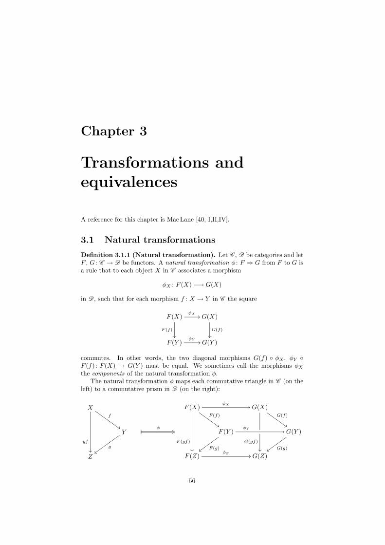
Chapter 3
Transformations and
equivalences
A reference for this chapter is Mac Lane [40, I,II,IV].
3.1 Natural transformations
Definition 3.1.1 (Natural transformation). Let C , D be categories and letF , G : C → D be functors. A natural transformation φ : F ⇒ G from F to G isa rule that to each object X in C associates a morphism
φX : F (X) −→ G(X)
in D , such that for each morphism f : X → Y in C the square
F (X)φX //
F (f)
²²
G(X)
G(f)
²²
F (Y )φY // G(Y )
commutes. In other words, the two diagonal morphisms G(f) φX , φY F (f) : F (X) → G(Y ) must be equal. We sometimes call the morphisms φX
the components of the natural transformation φ.The natural transformation φ maps each commutative triangle in C (on the
left) to a commutative prism in D (on the right):
Xf
##HHHHHHHHHH
gf
²²
F (X)φX //
F (f)
##HHHHHHHH
F (gf)
²²
G(X)G(f)
##HHHHHHHH
G(gf)
²²
Y
gvvvvvvvvvv
ÂÂ φ +3 F (Y )φY //
F (g)vvvvvvv
vG(Y )
G(g)vvvvvvvv
Z F (Z)φZ // G(Z)
56
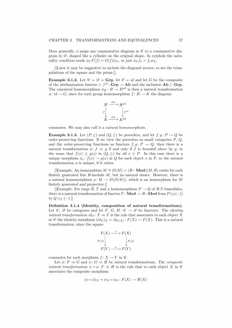
CHAPTER 3. TRANSFORMATIONS AND EQUIVALENCES 57
More generally, φ maps any commutative diagram in C to a commutative dia-gram in D , shaped like a cylinder on the original shape. In symbols the natu-rality condition reads φY F (f) = G(f)φX , or just φY f∗ = f∗φX .
[[Later it may be suggestive to include the diagonal arrows, to see the trian-gulations of the square and the prism.]]
Example 3.1.2. Let C = D = Grp, let F = id and let G be the compositeof the abelianization functor (−)ab : Grp → Ab and the inclusion Ab ⊂ Grp.The canonical homomorphism φH : H → Hab is then a natural transformationφ : id → G, since for each group homomorphism f : H → K the diagram
HφH //
f
²²
Hab
fab
²²
KφK // Kab
commutes. We may also call it a natural homomorphism.
Example 3.1.3. Let (P,≤) and (Q,≤) be preorders, and let f, g : P → Q beorder-preserving functions. If we view the preorders as small categories P , Q,and the order-preserving functions as functors f, g : P → Q, then there is anatural transformation φ : f ⇒ g if and only if f is bounded above by g, inthe sense that f(x) ≤ g(x) in (Q,≤) for all x ∈ P . In this case there is aunique morphism φx : f(x) → g(x) in Q for each object x in P , so the naturaltransformation φ is unique, if it exists.
[[Example: An isomorphism M ∼= D(M) = (R−Mod)(M,R) exists for eachfinitely generated free R-module M , but no natural choice. However, there isa natural homomorphism ρ : M → D(D(M)), which is an isomorphism for Mfinitely generated and projective.]]
[[Example: For rings R, T and a homomorphism P → Q of R-T -bimodules,there is a natural transformation of functor T−Mod → R−Mod from P⊗T (−))to Q ⊗T (−).]]
Definition 3.1.4 (Identity, composition of natural transformations).Let C , D be categories and let F , G, H : C → D be functors. The identitynatural transformation idF : F ⇒ F is the rule that associates to each object Xin C the identity morphism (idF )X = idF (X) : F (X) → F (X). This is a naturaltransformation, since the square
F (X)= //
F (f)
²²
F (X)
F (f)
²²
F (Y )= // F (Y )
commutes for each morphism f : X → Y in C .Let φ : F ⇒ G and ψ : G ⇒ H be natural transformations. The composite
natural transformation ψ φ : F ⇒ H is the rule that to each object X in C
associates the composite morphism
(ψ φ)X = ψX φX : F (X) → H(X)
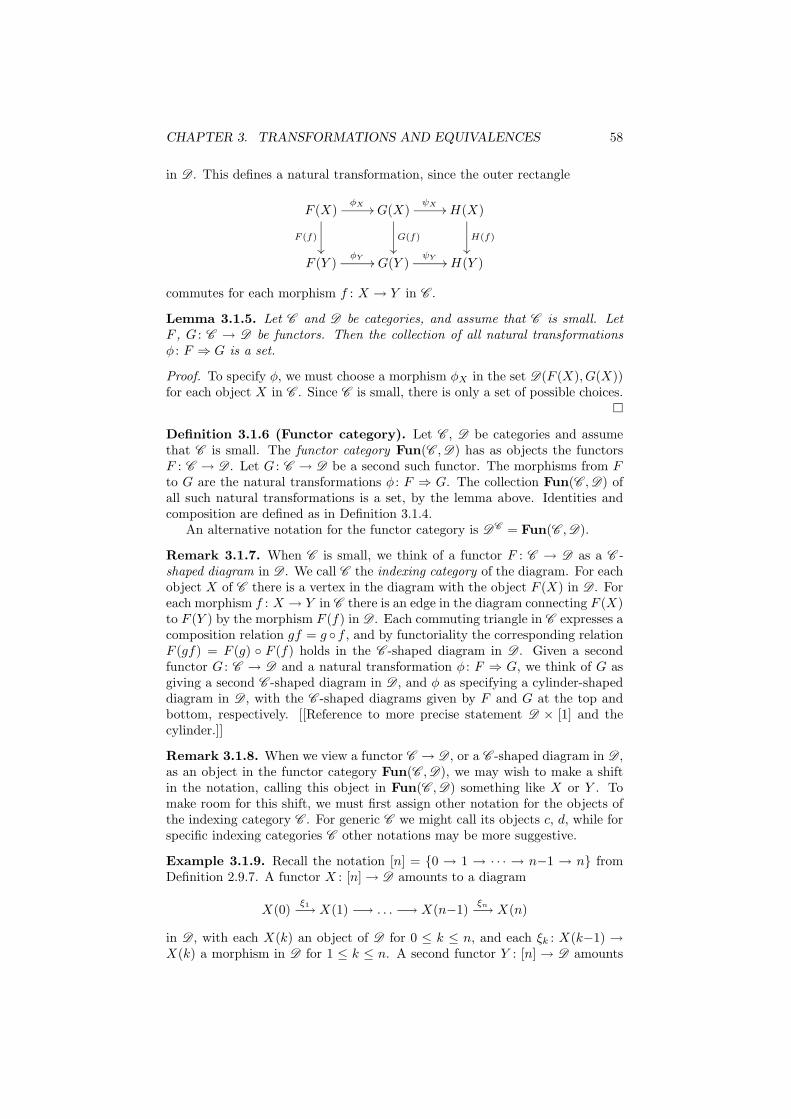
CHAPTER 3. TRANSFORMATIONS AND EQUIVALENCES 58
in D . This defines a natural transformation, since the outer rectangle
F (X)φX //
F (f)
²²
G(X)ψX //
G(f)
²²
H(X)
H(f)
²²
F (Y )φY // G(Y )
ψY // H(Y )
commutes for each morphism f : X → Y in C .
Lemma 3.1.5. Let C and D be categories, and assume that C is small. LetF , G : C → D be functors. Then the collection of all natural transformationsφ : F ⇒ G is a set.
Proof. To specify φ, we must choose a morphism φX in the set D(F (X), G(X))for each object X in C . Since C is small, there is only a set of possible choices.
Definition 3.1.6 (Functor category). Let C , D be categories and assumethat C is small. The functor category Fun(C ,D) has as objects the functorsF : C → D . Let G : C → D be a second such functor. The morphisms from Fto G are the natural transformations φ : F ⇒ G. The collection Fun(C ,D) ofall such natural transformations is a set, by the lemma above. Identities andcomposition are defined as in Definition 3.1.4.
An alternative notation for the functor category is DC = Fun(C ,D).
Remark 3.1.7. When C is small, we think of a functor F : C → D as a C -shaped diagram in D . We call C the indexing category of the diagram. For eachobject X of C there is a vertex in the diagram with the object F (X) in D . Foreach morphism f : X → Y in C there is an edge in the diagram connecting F (X)to F (Y ) by the morphism F (f) in D . Each commuting triangle in C expresses acomposition relation gf = g f , and by functoriality the corresponding relationF (gf) = F (g) F (f) holds in the C -shaped diagram in D . Given a secondfunctor G : C → D and a natural transformation φ : F ⇒ G, we think of G asgiving a second C -shaped diagram in D , and φ as specifying a cylinder-shapeddiagram in D , with the C -shaped diagrams given by F and G at the top andbottom, respectively. [[Reference to more precise statement D × [1] and thecylinder.]]
Remark 3.1.8. When we view a functor C → D , or a C -shaped diagram in D ,as an object in the functor category Fun(C ,D), we may wish to make a shiftin the notation, calling this object in Fun(C ,D) something like X or Y . Tomake room for this shift, we must first assign other notation for the objects ofthe indexing category C . For generic C we might call its objects c, d, while forspecific indexing categories C other notations may be more suggestive.
Example 3.1.9. Recall the notation [n] = 0 → 1 → · · · → n−1 → n fromDefinition 2.9.7. A functor X : [n] → D amounts to a diagram
X(0)ξ1−→ X(1) −→ . . . −→ X(n−1)
ξn−→ X(n)
in D , with each X(k) an object of D for 0 ≤ k ≤ n, and each ξk : X(k−1) →X(k) a morphism in D for 1 ≤ k ≤ n. A second functor Y : [n] → D amounts
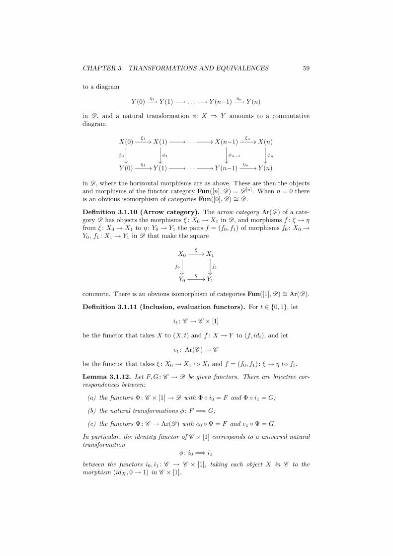
CHAPTER 3. TRANSFORMATIONS AND EQUIVALENCES 59
to a diagram
Y (0)η1−→ Y (1) −→ . . . −→ Y (n−1)
ηn−→ Y (n)
in D , and a natural transformation φ : X ⇒ Y amounts to a commutativediagram
X(0)ξ1 //
φ0
²²
X(1) //
φ1
²²
. . . // X(n−1)ξn //
φn−1
²²
X(n)
φn
²²
Y (0)η1 // Y (1) // . . . // Y (n−1)
ηn // Y (n)
in D , where the horizontal morphisms are as above. These are then the objectsand morphisms of the functor category Fun([n],D) = D [n]. When n = 0 thereis an obvious isomorphism of categories Fun([0],D) ∼= D .
Definition 3.1.10 (Arrow category). The arrow category Ar(D) of a cate-gory D has objects the morphisms ξ : X0 → X1 in D , and morphisms f : ξ → ηfrom ξ : X0 → X1 to η : Y0 → Y1 the pairs f = (f0, f1) of morphisms f0 : X0 →Y0, f1 : X1 → Y1 in D that make the square
X0ξ
//
f0
²²
X1
f1
²²
Y0η
// Y1
commute. There is an obvious isomorphism of categories Fun([1],D) ∼= Ar(D).
Definition 3.1.11 (Inclusion, evaluation functors). For t ∈ 0, 1, let
it : C → C × [1]
be the functor that takes X to (X, t) and f : X → Y to (f, idt), and let
et : Ar(C ) → C
be the functor that takes ξ : X0 → X1 to Xt and f = (f0, f1) : ξ → η to ft.
Lemma 3.1.12. Let F,G : C → D be given functors. There are bijective cor-respondences between:
(a) the functors Φ: C × [1] → D with Φ i0 = F and Φ i1 = G;
(b) the natural transformations φ : F =⇒ G;
(c) the functors Ψ: C → Ar(D) with e0 Ψ = F and e1 Ψ = G.
In particular, the identity functor of C × [1] corresponds to a universal naturaltransformation
φ : i0 =⇒ i1
between the functors i0, i1 : C → C × [1], taking each object X in C to themorphism (idX , 0 → 1) in C × [1].
CHAPTER 3. TRANSFORMATIONS AND EQUIVALENCES 60
Proof. The first correspondence takes a functor Φ to the natural transformationφ with φX = Φ(idX , 0 → 1). Conversely, a natural transformation φ maps tothe functor Φ given on objects by Φ(X, 0) = F (X), Φ(X, 1) = G(X), and onmorphisms by Φ(f, id0) = F (f), Φ(f, id1) = G(f) and Φ(idX , 0 → 1) = ψX .The commutation relation
(idY , 0 → 1) (f, id0) = (f, 0 → 1) = (f, id1) (idX , 0 → 1)
in the product category C × [1] corresponds precisely to the naturality conditionon φ.
The second correspondence takes a natural transformation φ to the functorΨ given on objects by Ψ(X) = (φX : F (X) → G(X)), and on morphisms byΨ(f) = (F (f), G(f)). Conversely, a functor Ψ maps to the natural transforma-tion φ with φX = Ψ(X). The commutation condition for morphisms in Ar(D)corresponds precisely to the naturality condition on φ.
Lemma 3.1.13. Let C , D , E be categories, with C and D small. There is anatural isomorphism
Fun(C × D ,E ) ∼= Fun(C ,Fun(D ,E ))
that takes a functor Φ: C × D → E to the functor Ψ: C → Fun(D ,E ) thattakes X in C to Ψ(X) : D → E given by Ψ(X)(Y ) = Φ(X,Y ) for all Y in D .
Proof. [[Clear enough.]]
3.2 Natural isomorphisms and equivalences
Definition 3.2.1 (Natural isomorphism). Let C , D be categories and let
F , G : C → D be functors. A natural isomorphism φ : F∼=
=⇒ G is a naturaltransformation such that the morphism
φX : F (X)∼=−→ G(X)
is an isomorphism in D , for each object X in C . Alternatively we may writeφ : F ∼= G.
Example 3.2.2. Let C , D be categories with obj(C ) = obj(D) = ∗, andendomorphism monoids M = C (∗, ∗), N = D(∗, ∗), let F,G : C → D be func-tors with associated monoid homomorphisms F,G : M → N , and let φ : F ⇒ Gbe a natural transformation. Then φ associates to the object ∗ in C a mor-phism φ∗ : ∗ = F (∗) → G(∗) = ∗ in D , which we consider as an elementh = φ∗ ∈ N = D(∗, ∗). The condition that φ is a natural transformation asksthat hF (f) = G(f)h in N , for all f ∈ M . We say that h ∈ N acts as an inter-twiner between the homomorphisms F : M → N and G : M → N . When φ is anatural isomorphism, h must be invertible in N , so the naturality condition canbe rewritten as G(f) = hF (f)h−1 for all f ∈ M . In other words, G : M → N isthe conjugate of F : M → N by h.
Similar remarks apply when C , D are one-object groupoids, and φ : F ⇒ Ga natural transformation of functors F , G : C → D . Since D is a groupoid, φ isautomatically a natural isomorphism.
CHAPTER 3. TRANSFORMATIONS AND EQUIVALENCES 61
Lemma 3.2.3. The identity idF : F∼=
=⇒ F is a natural isomorphism, the in-
verse φ−1 : G∼=
=⇒ F of a natural isomorphism is a natural isomorphism, and
the composite ψ φ : F∼=
=⇒ H of φ and a natural isomorphism ψ : G∼=
=⇒ is anatural isomorphism.
Proof. This is clear.
Lemma 3.2.4. A natural transformation φ : F ⇒ G is a natural isomorphismif and only if there exists a natural transformation ψ : G ⇒ F such that ψ φ =idF and φ ψ = idG. If C is small, this is the same as saying that φ is anisomorphism from F to G in Fun(C ,D).
Proof. Suppose that φ is a natural isomorphisms, so that φX : F (X) → G(X)is an isomorphism for each object X in C . Let ψX = (φX)−1 : G(X) → F (X)be the inverse isomorphism, for each X. Then the square
G(X)ψX //
G(f)
²²
F (X)
F (f)
²²
G(Y )ψY // F (Y )
commutes for each morphism f : X → Y , because
F (f) ψX = ψY φY F (f) φ−1X = ψY G(f)φX φ−1
X = ψY G(f) .
Hence ψ is a natural transformation. It is clear that ψφ and φψ are the respectiveidentity transformations.
Example 3.2.5. A natural isomorphism φ : X∼=
=⇒ Y between a pair of functorsX, Y : [n] → D amounts to a commutative diagram
X(0)ξ1 //
φ0∼=
²²
X(1) //
φ1∼=
²²
. . . // X(n−1)ξn //
φn−1∼=
²²
X(n)
φn∼=
²²
Y (0)η1 // Y (1) // . . . // Y (n−1)
ηn // Y (n)
in D , where the vertical arrows are isomorphisms.
[[Example: Natural transformation νM : HomR(P,R)⊗RM → HomR(P,M)is a natural isomorphism when P is finitely generated and projective.]]
[[Natural transformation ρM : M → HomR(HomR(M,R), R) is a natural iso-morphism when restricted to the full subcategory of finitely generated projectiveR-modules M ]]
Remark 3.2.6. Recall that an isomorphism of categories is a functor F : C →D such that there exists an inverse functor G : D → C with GF = idC : C → C
and F G = idD : D → D . Requiring equality of functors in these two casesis a very strict condition. It is more natural in the categorical context to askfor natural isomorphism of functors. This leads to the following notion, ofequivalence of categories, which is a more flexible and useful condition.
CHAPTER 3. TRANSFORMATIONS AND EQUIVALENCES 62
Definition 3.2.7 (Equivalence of categories). Let C , D be categories. Afunctor F : C → D is an equivalence if there exists a functor G : D → C and
natural isomorphisms φ : G F∼=
=⇒ idC and ψ : F G∼=
=⇒ idD .In this case we say that C and D are equivalent categories, and that G is an
inverse equivalence to F . Note that G is usually not uniquely determined by F .It does of course not matter if we specify the natural isomorphisms φ and ψ ortheir inverses.
Lemma 3.2.8. Equivalence of categories defines an equivalence relation on anyset of categories.
Proof. The identity idC : C → C is clearly an equivalence of categories. If
F : C → D and G : D → C satisfy GF∼=
=⇒ idC and FG∼=
=⇒ idD , so thatF is an equivalence, then the same natural isomorphisms show that G is an
equivalence. If furthermore F ′ : D → E and G′ : E → D satisfy G′F ′∼=
=⇒ idD
and F ′G′∼=
=⇒ idE , so that F and F ′ are equivalences, then F ′F : C → E is alsoan equivalence, since there are composite natural isomorphisms
(GG′)(F ′F ) = G(G′F ′)F∼=
=⇒ G(idD)F = GF∼=
=⇒ idC
and(F ′F )(GG′) = F ′(FG)G′ ∼=
=⇒ F ′(idD)G′ = F ′G′ ∼==⇒ idE .
Definition 3.2.9 (Essentially surjective functor). A functor F : C → D
is essentially surjective if for each object Z of D there exists an object X of C
and an isomorphism F (X) ∼= Z in D .
Theorem 3.2.10. A functor F : C → D is an equivalence of categories if andonly if it is a full, faithful and essentially surjective.
Proof. For the forward implication, suppose that F is an equivalence. Then
there exists a functor G : D → C and natural isomorphisms φ : GF∼=
=⇒ idC
and ψ : FG∼=
=⇒ idD . Consider any pair of objects X, Y in C , and consider thefunction
F : C (X,Y ) −→ D(F (X), F (Y ))
taking f to F (f). We must prove that it is a bijection, so that F is full andfaithful. First, consider two morphisms f, g : X → Y in C , and suppose thatF (f) = F (g) in D . Then GF (f) = GF (g) in C , so we can combine the followingtwo commutative squares:
X
f
²²
GF (X)φX
∼=oo
φX
∼=//
GF (f)=GF (g)
²²
X
g
²²
Y GF (Y )φY
∼=oo
φY
∼=// Y
Hence f = φY φ−1Y g φXφ−1
X = g and the function F is injective. By the same
argument, using ψ : FG∼=
=⇒ idD , the function
G : D(Z,W ) −→ C (G(Z), G(W ))
CHAPTER 3. TRANSFORMATIONS AND EQUIVALENCES 63
is injective for all objects Z, W in D . Next, let h : F (X) → F (Y ) be a morphismin D . Form the composite morphism f = φY G(h) φ−1
X in C . Then we havethe following two commutative squares:
GF (X)φX
∼=//
G(h)
²²
X
f
²²
GF (X)φX
∼=oo
GF (f)
²²
GF (Y )φY
∼=// Y GF (Y )
φY
∼=oo
Hence G(h) = φ−1Y φY GF (f) φ−1
X φX = GF (f). By injectivity of the func-tion G, it follows that h = F (f). Since h : F (X) → F (Y ) was arbitrary, thisproves that the function F is surjective. Finally, given any object Z of D let
X = G(Z). Then ψZ : FG(Z)∼=−→ Z is an isomorphism F (X) ∼= Z. Hence F is
essentially surjective.For the reverse implication, suppose that F is full, faithful and essentially
surjective. We must construct an inverse equivalence G : D → C . For eachobject Z in D there exists an object X in C such that F (X) ∼= Z, by theessential surjectivity of F . For each Z we fix such an object X, and defineG(Z) = X. This specifies G on objects. Furthermore, for each Z we choose an
isomorphism F (X)∼=−→ Z, which we denote ψZ : FG(Z)
∼=−→ Z. This specifies
a natural isomorphism ψ : FG → idD on objects. Now let h : Z → W be amorphism in D . The composite ψ−1
W h ψZ : FG(Z) → FG(W ) in D can bewritten as F (f) for a unique morphism f : G(Z) → G(W ), since F is full andfaithful. We define G(h) = f for this unique morphism. This specifies G onmorphisms. It is straightforward to check that G : D → C is a functor. Thediagram
FG(Z)ψZ
∼=//
FG(h)
²²
Z
h
²²
FG(W )ψW
∼=// W
commutes, since FG(h) = F (f) = ψ−1W h ψZ , so ψ : FG
∼=−→ idD is a natural
isomorphism. It remains to construct a natural isomorphism φ : GF∼=
=⇒ idC .
For each object X in C , the isomorphism ψF (X) : FGF (X)∼=−→ F (X) can be
written as F (φX) for a unique morphism φX : GF (X) → X, since F is full andfaithful. This specifies φ on objects. Finally, let f : X → Y be a morphismin C . We must verify that the square
GF (X)φX
∼=//
GF (f)
²²
X
f
²²
GF (Y )φY
∼=// Y
commutes. Since F is faithful, it suffices to show that F (f φX) = F (f) F (φX) = F (f) ψF (X) is equal to F (φY GF (f)) = F (φY ) FGF (f) =
ψF (Y ) FGF (f), but this is just the naturality condition for ψ : FG∼=
=⇒ idD
with respect to the morphism F (f) : F (X) → F (Y ) in D .
CHAPTER 3. TRANSFORMATIONS AND EQUIVALENCES 64
Elaborating on Definition 2.8.1, we use the following terminology.
Definition 3.2.11 (Skeletal subcategory). A skeleton of a category C isa full subcategory C ′ ⊆ C such that each object of C is isomorphic in C toone and only one object in C ′. (We do not ask that the isomorphism is uniqueas a morphism in C .) The subcategory C ′ is then skeletal, in the sense thattwo objects X, Y in C ′ are isomorphic in C ′ if and only if they are equal. Acategory C is said to be skeletally small if it admits a skeleton C ′ that is small.
Lemma 3.2.12. The inclusion of a skeleton C ′ in a category C is an equiva-lence of categories.
Proof. The inclusion functor C ′ ⊆ C is full and faithful, since C ′ is a fullsubcategory. Furthermore, this functor is essentially surjective, by the definitionof a skeleton. Hence it is an equivalence of categories, by Theorem 3.2.10.
Example 3.2.13. The category F of Example 2.2.8 is a small skeleton of thecategory Fin of finite sets and functions. Similarly, the groupoid iso(F ) is asmall skeleton of iso(Fin).
Lemma 3.2.14. Any two skeleta of the same category are isomorphic.
Proof. Let C ′ and C ′′ be skeleta of C . For each object X ′ of C ′, there is a uniqueobject X ′′ in C ′′ such that X ′ and X ′′ are isomorphic in C . Choose such an
isomorphism hX′ : X ′∼=−→ X ′′. Define a functor F : C ′ → C ′′ by F (X ′) = X ′′
on objects. For any morphism f ′ : X ′ → Y ′ in C ′, let F (f ′) : X ′′ → Y ′′ be thecomposite
F (f ′) = hY ′ f ′ h−1X′ .
Then F (idX′) = idX′′ and F (g′f ′) = F (g′)F (f ′) whenever f ′ and g′ : Y ′ → Z ′
are composable, so F is a functor.Reversing the roles of C ′ and C ′′, we can also define a functor G : C ′′ →
C ′. Then GF (X ′) = X ′ and FG(X ′′) = X ′′. If we take care to choose the
isomorphism h−1X′ : X ′′
∼=−→ X ′ as the isomorphism hX′′ in the definition of G on
morphisms, then we also get that GF (f ′) = f ′ and FG(f ′′) = f ′′, so F and Gare inverse isomorphisms of categories.
Definition 3.2.15 (Connected groupoid). We say that a groupoid C isconnected if it is non-empty, and any two objects X,Y ∈ obj(C ) are isomorphic.A connected, skeletal groupoid has precisely one object.
Lemma 3.2.16. Let X be an object in a connected groupoid C , with automor-phism group Aut(X) = C (X,X). Then the inclusion
B Aut(X) = BC (X,X)≃−→ C
is an equivalence of categories.
Proof. We identify BC (X,X) with the full subgroupoid of C generated bythe object X. The inclusion functor is obviously full and faithful, and it isessentially surjective since C is assumed to be connected. Hence the inclusionis an equivalence, by Theorem 3.2.10.
CHAPTER 3. TRANSFORMATIONS AND EQUIVALENCES 65
Proposition 3.2.17. Let C be a groupoid with a small skeleton C ′, generatedby a set Xii∈I of objects. The inclusion
∐
i∈I
B Aut(Xi) =∐
i∈I
BC (Xi,Xi) ∼= C′ ≃−→ C
is an equivalence of categories.
Proof. Let Ci ⊆ C be the full subgroupoid of C generated by the objects thatare isomorphic to Xi, for each i ∈ I. Then there is an isomorphism of categories
∐
i∈I
Ci∼= C .
Each Ci is connected, so there is an equivalence B Aut(Xi) = BC (Xi,Xi) ≃ Ci
by Lemma 3.2.16. The coproduct of these equivalences is the asserted equiva-lence.
Example 3.2.18. Let C be a non-empty groupoid such that any two objectsare isomorphic by a unique isomorphism. Then Aut(X) = idX for each objectX in C , and the unique functor
C≃−→ ∗
to the terminal category is an equivalence.
Example 3.2.19. The groupoid iso(Fin) of finite sets has the small skeletonF , generated by the objects n = 1, 2, . . . n for n ∈ N0, and Aut(n) = Σn, sothe inclusion ∐
n≥0
BΣn≃−→ iso(Fin)
is an equivalence of categories.
Example 3.2.20. Let G be a finite group. The groupoid iso(G−Fin) of finiteG-sets has a small skeleton generated by the objects
X(ν) =∐
(H)
ν(H)∐
i=1
G/H
where H ranges over a set of representatives for the conjugacy classes of sub-groups of G, and each ν(H) ∈ N0. The elements x ∈ X(ν) with stabilizer Gx
conjugate to H lie in the summand indexed by (H). A G-equivariant bijectionf : X(ν) → X(ν) preserves the stabilizers, in the sense that Gx = Gf(x), henceit decomposes as a coproduct f =
∐(H) fH . For each H, letting n = ν(H), the
restricted G-equivariant bijection
fH :n∐
i=1
G/H −→n∐
i=1
G/H
takes the i’th copy of G/H to the σ(i)-th copy of G/H, for some permutationσ ∈ Σn, and for each 1 ≤ i ≤ n, the G-map G/H → G/H is determined by
CHAPTER 3. TRANSFORMATIONS AND EQUIVALENCES 66
taking eH to wiH for some element wi ∈ WG(H). [[Reference for Weyl group?]]We can write
fH = (σ;w1, . . . , wn) ∈ Σn ⋉ WG(H) × · · · × WG(H) = Σn ≀ WG(H) .
[[Reference for wreath product?]] Hence
Aut(X(ν)) ∼=∏
(H)
Σν(H) ≀ WG(H)
and iso(G−Fin) is equivalent to the small skeleton
∐
ν
B Aut(X(ν)) ∼=∏
(H)
∐
n≥0
B(Σn ≀ WG(H)) .
Example 3.2.21. For G = Cp of prime order, the possible subgroups areH = G and H = e, with Weyl groups WG(G) = e and WG(e) = G, so
iso(Cp−Fin) ≃∐
n≥0
BΣn ×∐
n≥0
B(Σn ≀ G) .
[[Discuss functors Cp−Fin → Fin taking X to X, XG or X/G, and conversely.Give Segal–tom Dieck splitting.]]
3.3 Tannaka–Krein duality
We started by suggesting that we can study mathematical objects, such asgroups G and rings R, by means of their categories of representations, suchas the category G−Set of G-sets and the category R−Mod of R-modules. Anatural question is then to what extent these representation categories determinethe original object, i.e., can one recover the group G from the category G−Set,and can one recover the ring R from the category R−Mod?
This discussion is not critical for the development of algebraic K-theory,but has played an important role in Grothendieck’s ideas about motives, andmotivic cohomology is directly related to algebraic K-theory.
For compact abelian groups G, it suffices to consider the category of 1-dimensional complex G-representations G × C → C, or equivalently, the Pon-tryagin dual group G# = Hom(G, T). The group G is then recovered as thedouble dual group, since the natural homomorphism ρ : G → (G#)# is an iso-morphism.
For compact not-necessarily-abelian groups, a positive answer was given byTadao Tannaka [64], showing that G can be recovered from the category G−Vecof complex G-representations, together with its forgetful functor ω to the cat-egory Vec of complex vector spaces. Conversely, Mark Grigorievich Krein [35]characterized the additional structures present on a category for it to be equiv-alent to a category of G-representations. The resulting equivalence, betweencompact groups G and such Tannakian categories is known as Tannaka–Kreinduality.
We discuss the first part of this theory in the simpler case of discrete groups G,where it suffices to consider the category G−Set of discrete representations.
CHAPTER 3. TRANSFORMATIONS AND EQUIVALENCES 67
Definition 3.3.1 (Fiber functor). For a discrete group G, let the fiber functor
ω : G−Set → Set
be the forgetful functor, that takes a G-set X (with implicit action G×X → X)to the underlying set ω(X). Let Aut(ω) be the monoid of natural transforma-tions
φ : ω ⇒ ω
under composition. There is a homomorphism
τ : G → Aut(ω)
that takes g ∈ G to the natural transformation φ = τ(g) with componentsφX : ω(X) → ω(X) given by the function g·, mapping x ∈ ω(X) to gx ∈ ω(X).This is a natural transformation, since for each G-equivariant function f : X →Y the square
ω(X)g·
//
ω(f)
²²
ω(X)
ω(f)
²²
ω(Y )g·
// ω(Y )
commutes.
We can now recover G from the category G−Set, equipped with the fiberfunctor ω.
Proposition 3.3.2. The homomorphism τ : G → Aut(ω) is an isomorphism.In particular, Aut(ω) is a group and every natural transformation φ : ω ⇒ ω isa natural isomorphism.
Proof. We construct an inverse κ : Aut(ω) → G to τ . Given a natural trans-formation φ : ω ⇒ ω, consider its component φG : ω(G) → ω(G), at the G-setX = G, with the left action G×G → G given by the multiplication in G. Thiscomponent φG maps e ∈ ω(G) to some element φG(e) ∈ ω(G). We define κ(φ)to be this element:
κ(φ) = φG(e) .
For any g ∈ G it is clear that κτ(g) = ge = g. Conversely, consider anyφ ∈ Aut(ω). For each G-set X, and any element x ∈ ω(X), there is a unique G-equivariant function f : G → X with f(e) = x, given by the formula f(h) = hxfor h ∈ G. Chasing the element e ∈ ω(G) through the commutative diagram
ω(G)φG //
ω(f)
²²
ω(G)
ω(f)
²²
ω(X)φX // ω(X)
shows that φX(x) = φX(f(e)) = f(φG(e)) = f(g) = gx, so that φX = g·. Sincethis holds for all X, we see that φ = τκ(φ).
The terminology “fiber functor” is motivated by the following example.
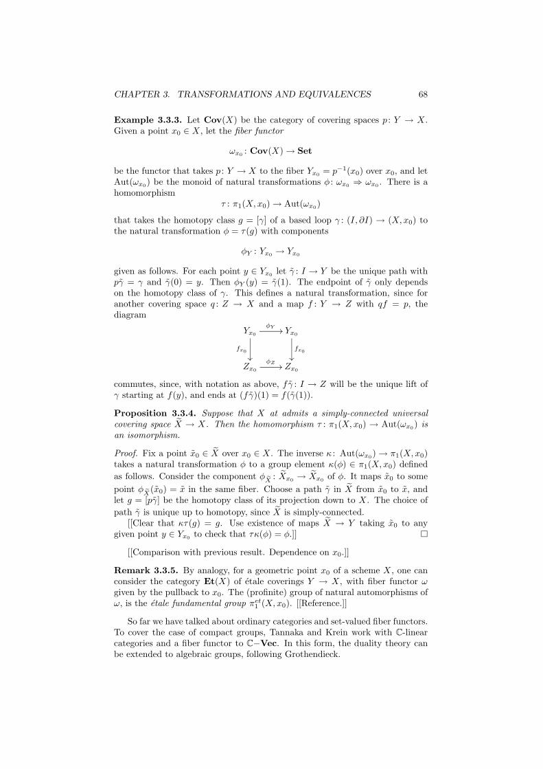
CHAPTER 3. TRANSFORMATIONS AND EQUIVALENCES 68
Example 3.3.3. Let Cov(X) be the category of covering spaces p : Y → X.Given a point x0 ∈ X, let the fiber functor
ωx0: Cov(X) → Set
be the functor that takes p : Y → X to the fiber Yx0= p−1(x0) over x0, and let
Aut(ωx0) be the monoid of natural transformations φ : ωx0
⇒ ωx0. There is a
homomorphismτ : π1(X,x0) → Aut(ωx0
)
that takes the homotopy class g = [γ] of a based loop γ : (I, ∂I) → (X,x0) tothe natural transformation φ = τ(g) with components
φY : Yx0→ Yx0
given as follows. For each point y ∈ Yx0let γ : I → Y be the unique path with
pγ = γ and γ(0) = y. Then φY (y) = γ(1). The endpoint of γ only dependson the homotopy class of γ. This defines a natural transformation, since foranother covering space q : Z → X and a map f : Y → Z with qf = p, thediagram
Yx0
φY //
fx0
²²
Yx0
fx0
²²
Zx0
φZ // Zx0
commutes, since, with notation as above, fγ : I → Z will be the unique lift ofγ starting at f(y), and ends at (fγ)(1) = f(γ(1)).
Proposition 3.3.4. Suppose that X at admits a simply-connected universalcovering space X → X. Then the homomorphism τ : π1(X,x0) → Aut(ωx0
) isan isomorphism.
Proof. Fix a point x0 ∈ X over x0 ∈ X. The inverse κ : Aut(ωx0) → π1(X,x0)
takes a natural transformation φ to a group element κ(φ) ∈ π1(X,x0) defined
as follows. Consider the component φ eX : Xx0→ Xx0
of φ. It maps x0 to some
point φ eX(x0) = x in the same fiber. Choose a path γ in X from x0 to x, andlet g = [pγ] be the homotopy class of its projection down to X. The choice of
path γ is unique up to homotopy, since X is simply-connected.[[Clear that κτ(g) = g. Use existence of maps X → Y taking x0 to any
given point y ∈ Yx0to check that τκ(φ) = φ.]]
[[Comparison with previous result. Dependence on x0.]]
Remark 3.3.5. By analogy, for a geometric point x0 of a scheme X, one canconsider the category Et(X) of etale coverings Y → X, with fiber functor ωgiven by the pullback to x0. The (profinite) group of natural automorphisms ofω, is the etale fundamental group πet
1 (X,x0). [[Reference.]]
So far we have talked about ordinary categories and set-valued fiber functors.To cover the case of compact groups, Tannaka and Krein work with C-linearcategories and a fiber functor to C−Vec. In this form, the duality theory canbe extended to algebraic groups, following Grothendieck.
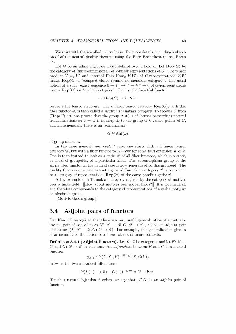
CHAPTER 3. TRANSFORMATIONS AND EQUIVALENCES 69
We start with the so-called neutral case. For more details, including a sketchproof of the neutral duality theorem using the Barr–Beck theorem, see Breen[9].
Let G be an affine algebraic group defined over a field k. Let Rep(G) bethe category of (finite-dimensional) of k-linear representations of G. The tensorproduct V ⊗k W and internal Hom Homk(V,W ) of G-representations V,Wmakes Rep(G) a “compact closed symmetric monoidal category”. The usualnotion of a short exact sequence 0 → V ′ → V → V ′′ → 0 of G-representationsmakes Rep(G) an “abelian category”. Finally, the forgetful functor
ω : Rep(G) → k−Vec
respects the tensor structure. The k-linear tensor category Rep(G), with thisfiber functor ω, is then called a neutral Tannakian category. To recover G from(Rep(G), ω), one proves that the group Aut(ω) of (tensor-preserving) naturaltransformations φ : ω ⇒ ω is isomorphic to the group of k-valued points of G,and more generally there is an isomorphism
G ∼= Aut(ω)
of group schemes.In the more general, non-neutral case, one starts with a k-linear tensor
category C , but with a fiber functor to K−Vec for some field extension K of k.One is then instead to look at a gerbe G of all fiber functors, which is a stack,or sheaf of groupoids, of a particular kind. The automorphism group of thesingle fiber functor in the neutral case is now generalized to this groupoid. Theduality theorem now asserts that a general Tannakian category C is equivalentto a category of representations Rep(G ) of the corresponding gerbe G .
A key example of a Tannakian category is given by the category of motivesover a finite field. [[How about motives over global fields?]] It is not neutral,and therefore corresponds to the category of representations of a gerbe, not justan algebraic group.
[[Motivic Galois group.]]
3.4 Adjoint pairs of functors
Dan Kan [33] recognized that there is a very useful generalization of a mutuallyinverse pair of equivalences (F : C → D , G : D → C ), called an adjoint pairof functors (F : C → D , G : D → C ). For example, this generalization gives aclear meaning to the notion of a “free” object in many contexts.
Definition 3.4.1 (Adjoint functors). Let C , D be categories and let F : C →D and G : D → C be functors. An adjunction between F and G is a naturalbijection
φX,Y : D(F (X), Y )∼=−→ C (X,G(Y ))
between the two set-valued bifunctors
D(F (−),−),C (−, G(−)) : Cop × D → Set .
If such a natural bijection φ exists, we say that (F,G) is an adjoint pair offunctors.
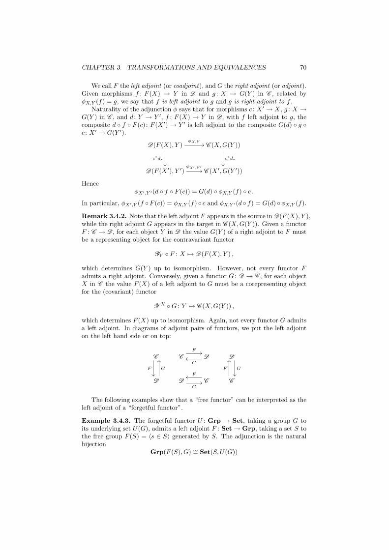
CHAPTER 3. TRANSFORMATIONS AND EQUIVALENCES 70
We call F the left adjoint (or coadjoint), and G the right adjoint (or adjoint).Given morphisms f : F (X) → Y in D and g : X → G(Y ) in C , related byφX,Y (f) = g, we say that f is left adjoint to g and g is right adjoint to f .
Naturality of the adjunction φ says that for morphisms c : X ′ → X, g : X →G(Y ) in C , and d : Y → Y ′, f : F (X) → Y in D , with f left adjoint to g, thecomposite d f F (c) : F (X ′) → Y ′ is left adjoint to the composite G(d) g c : X ′ → G(Y ′).
D(F (X), Y )φX,Y
//
c∗d∗
²²
C (X,G(Y ))
c∗d∗
²²
D(F (X ′), Y ′)φX′,Y ′
// C (X ′, G(Y ′))
HenceφX′,Y ′(d f F (c)) = G(d) φX,Y (f) c .
In particular, φX′,Y (f F (c)) = φX,Y (f) c and φX,Y ′(d f) = G(d) φX,Y (f).
Remark 3.4.2. Note that the left adjoint F appears in the source in D(F (X), Y ),while the right adjoint G appears in the target in C (X,G(Y )). Given a functorF : C → D , for each object Y in D the value G(Y ) of a right adjoint to F mustbe a representing object for the contravariant functor
YY F : X 7→ D(F (X), Y ) ,
which determines G(Y ) up to isomorphism. However, not every functor Fadmits a right adjoint. Conversely, given a functor G : D → C , for each objectX in C the value F (X) of a left adjoint to G must be a corepresenting objectfor the (covariant) functor
YX G : Y 7→ C (X,G(Y )) ,
which determines F (X) up to isomorphism. Again, not every functor G admitsa left adjoint. In diagrams of adjoint pairs of functors, we put the left adjointon the left hand side or on top:
C
F
²²
C
F //D
Goo D
G
²²
D
G
OO
DG
// C
FooC
F
OO
The following examples show that a “free functor” can be interpreted as theleft adjoint of a “forgetful functor”.
Example 3.4.3. The forgetful functor U : Grp → Set, taking a group G toits underlying set U(G), admits a left adjoint F : Set → Grp, taking a set S tothe free group F (S) = 〈s ∈ S〉 generated by S. The adjunction is the naturalbijection
Grp(F (S), G) ∼= Set(S,U(G))
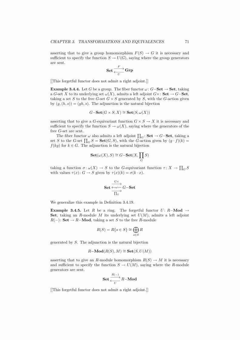
CHAPTER 3. TRANSFORMATIONS AND EQUIVALENCES 71
asserting that to give a group homomorphism F (S) → G it is necessary andsufficient to specify the function S → U(G), saying where the group generatorsare sent.
SetF //
GrpU
oo
[[This forgetful functor does not admit a right adjoint.]]
Example 3.4.4. Let G be a group. The fiber functor ω : G−Set → Set, takinga G-set X to its underlying set ω(X), admits a left adjoint G× : Set → G−Set,taking a set S to the free G-set G× S generated by S, with the G-action givenby (g, (h, s)) = (gh, s). The adjunction is the natural bijection
G−Set(G × S,X) ∼= Set(S, ω(X))
asserting that to give a G-equivariant function G × S → X it is necessary andsufficient to specify the function S → ω(X), saying where the generators of thefree G-set are sent.
The fiber functor ω also admits a left adjoint∏
G : Set → G−Set, taking aset S to the G-set
∏G S = Set(G,S), with the G-action given by (g · f)(k) =
f(kg) for k ∈ G. The adjunction is the natural bijection
Set(ω(X), S) ∼= G−Set(X,∏
G
S)
taking a function σ : ω(X) → S to the G-equivariant function τ : X →∏
G Swith values τ(x) : G → S given by τ(x)(k) = σ(k · x).
Set
G×//
QG
//G−Setωoo
We generalize this example in Definition 3.4.19.
Example 3.4.5. Let R be a ring. The forgetful functor U : R−Mod →Set, taking an R-module M its underlying set U(M), admits a left adjointR(−) : Set → R−Mod, taking a set S to the free R-module
R(S) = Rs ∈ S ∼=⊕
s∈S
R
generated by S. The adjunction is the natural bijection
R−Mod(R(S),M) ∼= Set(S,U(M))
asserting that to give an R-module homomorphism R(S) → M it is necessaryand sufficient to specify the function S → U(M), saying where the R-modulegenerators are sent.
SetR(−)
//R−Mod
Uoo
[[This forgetful functor does not admit a right adjoint.]]
CHAPTER 3. TRANSFORMATIONS AND EQUIVALENCES 72
One may also forget less structure.
Example 3.4.6. The abelianization functor (−)ab : Grp → Ab is left adjointto the forgetful functor U : Ab → Grp. This is because giving an (abelian)group homomorphism Gab → A is equivalent to giving a group homomorphismG → U(A). [[This forgetful functor U has no right adjoint.]]
Example 3.4.7. Let CMon be the full subcategory of Mon generated by thecommutative monoids. The group completion functor K : CMon → Ab is leftadjoint to the forgetful functor U : Ab → CMon. This is because giving a grouphomomorphism K(M) → A is equivalent to giving a monoid homomorphismM → U(A).
This forgetful functor U has a right adjoint (−)× : CMon → Ab, takingM to the submonoid M× of invertible elements in M , which forms an abeliangroup. Each monoid homomorphism U(A) → M factors uniquely through agroup homomorphism A → M×.
Definition 3.4.8 (Group completion, units). In the non-commutative case,the forgetful functor U : Grp → Mon also has a left adjoint K : Mon → Grp,the group completion of non-commutative monoids. Given a monoid M we candescribe the group K(M) in terms of generators and relations as
K(M) = 〈[x] | [x][y] = [xy]〉 .
In words, we start with one generator [x] for each element x ∈ M , and addthe relation [x][y] = [xy] for each pair of elements x, y ∈ M . Here [x][y] is theproduct in the free group generated by the elements of M , and xy is the productin M . The relation [e] = e follows. The adjunction
Grp(K(M), G) ∼= Mon(M,U(G))
takes a group homomorphism f : K(M) → G to the monoid homomorphismg : M → U(G) given by g(x) = f([x]), and conversely. Later, we shall see thatK(M) is topologically realized as π1(BM), where the classifying space BMcontains a closed loop [x] for each x ∈ M , and a triangle [x|y] with edges [x],[y] and [xy] for each x, y ∈ M .
This forgetful functor U also has a right adjoint (−)× : Mon → Grp, againtaking a monoid M to the submonoid M× of invertible elements, which is agroup.
Definition 3.4.9 ((Co-)reflective subcategory). A subcategory C ⊆ D iscalled reflective when the inclusion functor U : C → D is a right adjoint, i.e.,it admits a left adjoint F : D → C . It is called coreflective when U is a leftadjoint, i.e., it admits a right adjoint G : D → C .
We often omit forgetful functors like U from the notation.
Example 3.4.10. CMon ⊂ Ab, CMon ⊂ Mon, Ab ⊂ Grp and Mon ⊂Grp are reflective subcategories. CMon ⊂ Ab and Mon ⊂ Grp are also
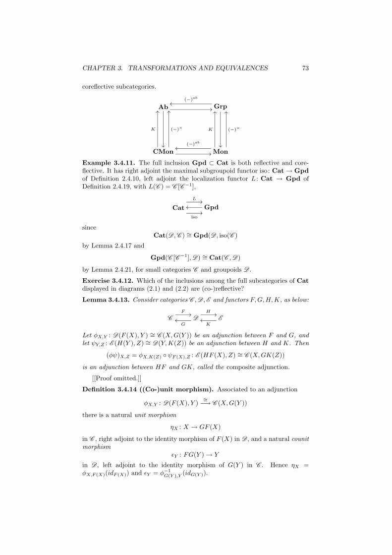
CHAPTER 3. TRANSFORMATIONS AND EQUIVALENCES 73
coreflective subcategories.
Ab //
²²
Grp(−)ab
oo
²²
CMon //
K
OO
(−)×
OO
Mon(−)ab
oo
K
OO
(−)×
OO
Example 3.4.11. The full inclusion Gpd ⊂ Cat is both reflective and core-flective. It has right adjoint the maximal subgroupoid functor iso : Cat → Gpdof Definition 2.4.10, left adjoint the localization functor L : Cat → Gpd ofDefinition 2.4.19, with L(C ) = C [C−1],
Cat
L //
iso//Gpdoo
sinceCat(D ,C ) ∼= Gpd(D , iso(C )
by Lemma 2.4.17 and
Gpd(C [C−1],D) ∼= Cat(C ,D)
by Lemma 2.4.21, for small categories C and groupoids D .
Exercise 3.4.12. Which of the inclusions among the full subcategories of Catdisplayed in diagrams (2.1) and (2.2) are (co-)reflective?
Lemma 3.4.13. Consider categories C ,D ,E and functors F,G,H,K, as below:
C
F //D
Goo
H //E
Koo
Let φX,Y : D(F (X), Y ) ∼= C (X,G(Y )) be an adjunction between F and G, andlet ψY,Z : E (H(Y ), Z) ∼= D(Y,K(Z)) be an adjunction between H and K. Then
(φψ)X,Z = φX,K(Z) ψF (X),Z : E (HF (X), Z) ∼= C (X,GK(Z))
is an adjunction between HF and GK, called the composite adjunction.
[[Proof omitted.]]
Definition 3.4.14 ((Co-)unit morphism). Associated to an adjunction
φX,Y : D(F (X), Y )∼=−→ C (X,G(Y ))
there is a natural unit morphism
ηX : X → GF (X)
in C , right adjoint to the identity morphism of F (X) in D , and a natural counitmorphism
ǫY : FG(Y ) → Y
in D , left adjoint to the identity morphism of G(Y ) in C . Hence ηX =φX,F (X)(idF (X)) and ǫY = φ−1
G(Y ),Y (idG(Y )).
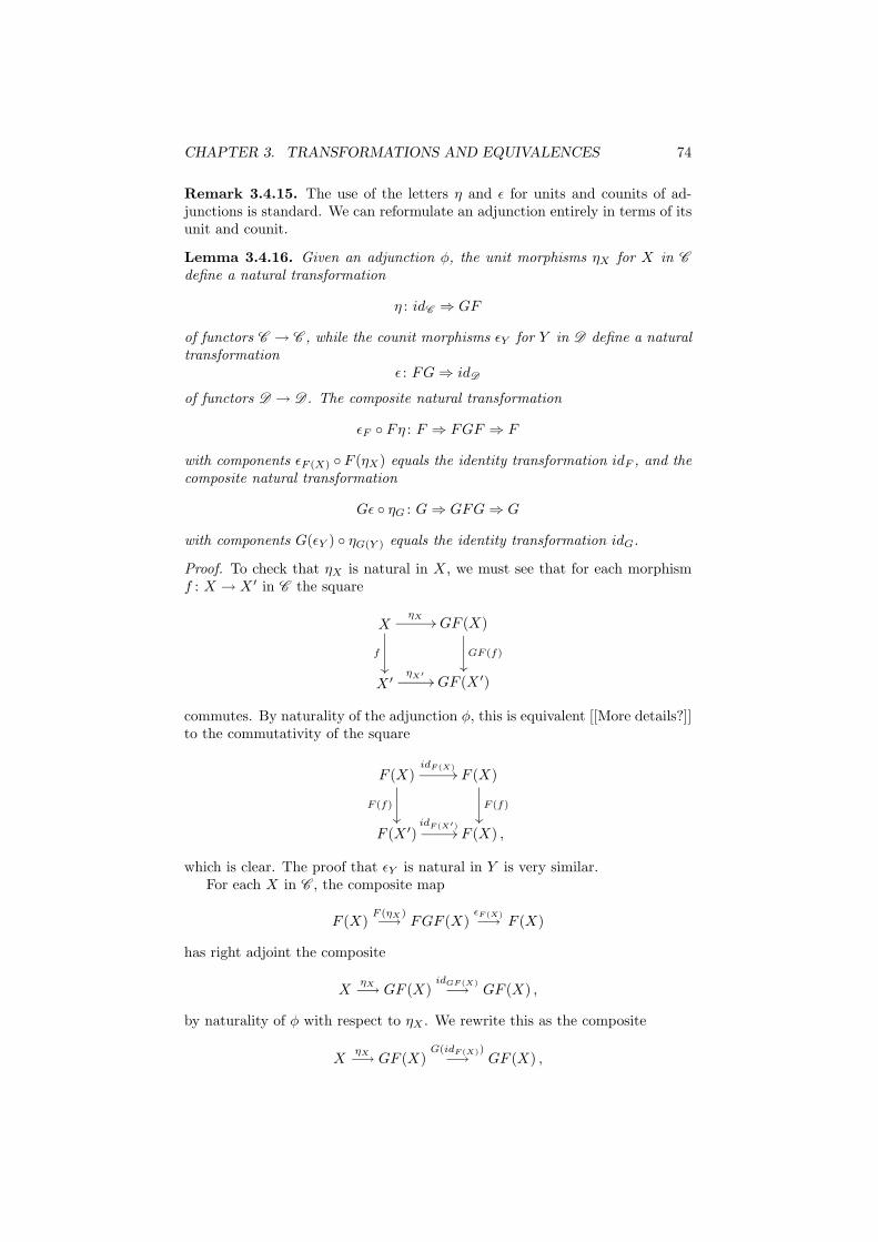
CHAPTER 3. TRANSFORMATIONS AND EQUIVALENCES 74
Remark 3.4.15. The use of the letters η and ǫ for units and counits of ad-junctions is standard. We can reformulate an adjunction entirely in terms of itsunit and counit.
Lemma 3.4.16. Given an adjunction φ, the unit morphisms ηX for X in C
define a natural transformation
η : idC ⇒ GF
of functors C → C , while the counit morphisms ǫY for Y in D define a naturaltransformation
ǫ : FG ⇒ idD
of functors D → D . The composite natural transformation
ǫF Fη : F ⇒ FGF ⇒ F
with components ǫF (X) F (ηX) equals the identity transformation idF , and thecomposite natural transformation
Gǫ ηG : G ⇒ GFG ⇒ G
with components G(ǫY ) ηG(Y ) equals the identity transformation idG.
Proof. To check that ηX is natural in X, we must see that for each morphismf : X → X ′ in C the square
XηX //
f
²²
GF (X)
GF (f)
²²
X ′ηX′
// GF (X ′)
commutes. By naturality of the adjunction φ, this is equivalent [[More details?]]to the commutativity of the square
F (X)idF (X)
//
F (f)
²²
F (X)
F (f)
²²
F (X ′)idF (X′)
// F (X) ,
which is clear. The proof that ǫY is natural in Y is very similar.For each X in C , the composite map
F (X)F (ηX)−→ FGF (X)
ǫF (X)−→ F (X)
has right adjoint the composite
XηX−→ GF (X)
idGF (X)−→ GF (X) ,
by naturality of φ with respect to ηX . We rewrite this as the composite
XηX−→ GF (X)
G(idF (X))−→ GF (X) ,
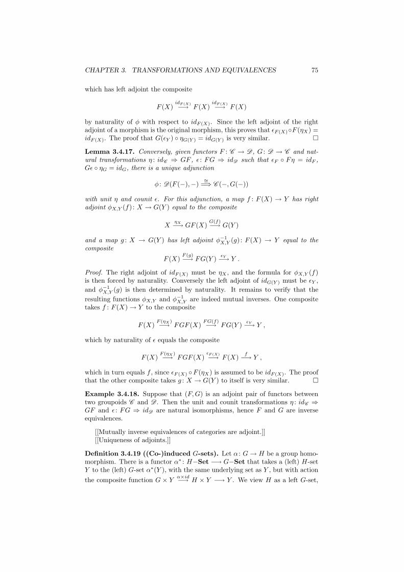
CHAPTER 3. TRANSFORMATIONS AND EQUIVALENCES 75
which has left adjoint the composite
F (X)idF (X)−→ F (X)
idF (X)−→ F (X)
by naturality of φ with respect to idF (X). Since the left adjoint of the rightadjoint of a morphism is the original morphism, this proves that ǫF (X)F (ηX) =idF (X). The proof that G(ǫY ) ηG(Y ) = idG(Y ) is very similar.
Lemma 3.4.17. Conversely, given functors F : C → D , G : D → C and nat-ural transformations η : idC ⇒ GF , ǫ : FG ⇒ idD such that ǫF Fη = idF ,Gǫ ηG = idG, there is a unique adjunction
φ : D(F (−),−)∼=
=⇒ C (−, G(−))
with unit η and counit ǫ. For this adjunction, a map f : F (X) → Y has rightadjoint φX,Y (f) : X → G(Y ) equal to the composite
XηX−→ GF (X)
G(f)−→ G(Y )
and a map g : X → G(Y ) has left adjoint φ−1X,Y (g) : F (X) → Y equal to the
composite
F (X)F (g)−→ FG(Y )
ǫY−→ Y .
Proof. The right adjoint of idF (X) must be ηX , and the formula for φX,Y (f)is then forced by naturality. Conversely the left adjoint of idG(Y ) must be ǫY ,
and φ−1X,Y (g) is then determined by naturality. It remains to verify that the
resulting functions φX,Y and φ−1X,Y are indeed mutual inverses. One composite
takes f : F (X) → Y to the composite
F (X)F (ηX)−→ FGF (X)
FG(f)−→ FG(Y )
ǫY−→ Y ,
which by naturality of ǫ equals the composite
F (X)F (ηX)−→ FGF (X)
ǫF (X)−→ F (X)
f−→ Y ,
which in turn equals f , since ǫF (X) F (ηX) is assumed to be idF (X). The proofthat the other composite takes g : X → G(Y ) to itself is very similar.
Example 3.4.18. Suppose that (F,G) is an adjoint pair of functors betweentwo groupoids C and D . Then the unit and counit transformations η : idC ⇒GF and ǫ : FG ⇒ idD are natural isomorphisms, hence F and G are inverseequivalences.
[[Mutually inverse equivalences of categories are adjoint.]][[Uniqueness of adjoints.]]
Definition 3.4.19 ((Co-)induced G-sets). Let α : G → H be a group homo-morphism. There is a functor α∗ : H−Set −→ G−Set that takes a (left) H-setY to the (left) G-set α∗(Y ), with the same underlying set as Y , but with action
the composite function G × Yα×id−→ H × Y −→ Y . We view H as a left G-set,
CHAPTER 3. TRANSFORMATIONS AND EQUIVALENCES 76
and as a right G-set, using α and the group multiplication in H. The functorα∗ has a left adjoint α∗ : G−Set −→ H−Set taking an G-set X to the H-set
α∗(X) = H ×G X ,
with action the function H ×H ×G Xµ×Gid−→ H ×G X. Here H ×G X denotes the
balanced product (H ×X)/∼, where (h · g, x) ∼ (h, g · x) for h ∈ H, g ∈ G andx ∈ X. The functor α∗ also has a right adjoint α! : G−Set −→ H−Set takingan G-set X to the H-set
α!(X) = G−Set(H,X) ,
of G-equivariant functions f : H → X. The H-action
H × G−Set(H,X) −→ G−Set(H,X)
on α!(X) takes (h, f) for h ∈ H, f ∈ G−Set(H,X) to the G-equivariant func-tion k 7→ f(kh), for k ∈ H.
G−Set
α∗ //
α!
//H−Setα∗oo
The adjunction bijections are:
H−Set(α∗(X), Y ) ∼= G−Set(X,α∗(Y ))
G−Set(α∗(Y ),X) ∼= H−Set(Y, α!(X))
Example 3.4.20. When α : e → H is the inclusion of the trivial subgroup,α∗ : H−Set → Set is the forgetful functor, equal to the fiber functor ω ofDefinition 3.3.1, the left adjoint α∗ takes a set X to the free H-set α∗(X) =H×X, and the right adjoint α! takes a set X to the cofree H-set α!(X) =
∏H X,
as discussed in Example 3.4.4.
Example 3.4.21. When α : G → e is the projection to the trivial group,α∗ : Set → G−Set takes a set X to the same set α∗(X), with the trivial G-action. The left adjoint α∗ takes an G-set Y to the orbit set
α∗(Y ) = e ×G Y ∼= Y/G .
The right adjoint α! takes Y to the fixed point set
α!(Y ) = G−Set(e, Y ) ∼= Y G .
See Definition 2.7.3 for this terminology.
Definition 3.4.22 (Direct and exceptional direct image). Let φ : R → Tbe a ring homomorphism. There is a functor φ∗ : T−Mod −→ R−Mod thattakes a (left) T -module N to the (left) R-module φ∗(N), with the same underly-ing abelian group as N , but with module action the composite homomorphism
R⊗Nφ⊗id−→ T⊗N −→ N . We view T as a left R-module and as a right R-module
using the homomorphism φ and the ring multiplication µ : T ⊗ T → T . The
CHAPTER 3. TRANSFORMATIONS AND EQUIVALENCES 77
functor φ∗ has a left adjoint φ∗ : R−Mod −→ T−Mod taking an R-module Mto the T -module
φ∗(M) = T ⊗R M ,
with module action the homomorphism T ⊗T ⊗RMµ⊗Rid−→ T ⊗RM . The functor
φ∗ also has a right adjoint φ! : R−Mod −→ T−Mod taking an R-module Mto the T -module
φ!(M) = RHom(T,M) ,
of R-module homomorphisms f : T → M , where T is viewed as an R-module
by the action R ⊗ Tφ⊗id−→ T ⊗ T
µ−→ T . The T -module structure
T ⊗ RHom(T,M) −→ RHom(T,M)
on φ!(M) takes t ⊗ f for t ∈ T , f ∈ RHom(T,M) to the R-module homomor-phism u 7→ f(ut), for u ∈ T .
R−Mod
φ∗ //
φ!
//T−Modφ∗oo
Both adjunctions
T−Mod(φ∗(M), N) ∼= R−Mod(M,φ∗(N))
R−Mod(φ∗(N),M) ∼= T−Mod(N,φ!(M))
respect the additive structure, hence lift to group isomorphisms
T Hom(T ⊗R M,N) ∼= RHom(M,φ∗(N))
RHom(φ∗(N),M) ∼= T Hom(N, RHom(T,M)) .
[[Warning: For R, T commutative, φ defines a morphism f : Spec(T ) →Spec(R) of schemes, and the induced functors inverse image f∗ = φ∗, directimage f∗ = φ∗ and exceptional inverse image f ! = φ! on quasi-coherent sheaves.Note the reversal in variance.]]
3.5 Decategorification
Definition 3.5.1. Let C be a small groupoid. We can define an equivalencerelation ∼= on the set of objects, obj(C ), by saying that X ∼= Y if there exists a
morphism (= an isomorphism) f : X∼=−→ Y from X to Y in C . The fact that
this is an equivalence relation follows easily from Lemma 2.4.3. Let the set ofequivalence classes
π0(C ) = obj(C )/ ∼=
be the set of isomorphism classes of objects in C . We write [X] ∈ π0(C ) forthe isomorphism class of an object X in C . By definition, [X] = Y ∈ obj(C ) |X ∼= Y .
CHAPTER 3. TRANSFORMATIONS AND EQUIVALENCES 78
Remark 3.5.2. Since the equivalence relation X ∼= Y only remembers theexistence of isomorphisms from X to Y in C , not the actual nonempty setof isomorphisms C (X,Y ), the set π0(C ) of isomorphism classes in C has losttrack of part of the categorical structure. We therefore refer to π0(C ) as thedecategorification of C . An important aspect of algebraic K-theory is a reversalof this process, attempting to lift set level structures to the category level, by aless well-defined process of categorification.
Example 3.5.3. Let N0 = 0, 1, 2, . . . be the set of non-negative integers.There is a bijection
π0(iso(F ))∼=−→ N0
that takes the object n to its cardinality n, for each n ≥ 0.
Remark 3.5.4. Under the bijection above, the disjoint union m ⊔ n and thecartesian product m×n give categorical models for the sum m+n and productmn of non-negative integers. In a sense, the need to count the number ofelements in the sets arising from these operations must have been one of theinitial reasons for introducing sums and products of natural numbers. Oncebookkeeping developed, it proved convenient to also introduce negative numbers,extending the number system from N0 to the integers Z = . . . ,−1, 0, 1, . . . .There are no sets with a negative number of elements, but what is a suitableextension the groupoid iso(F ), so that its π0 is naturally the ring of integers?[[We will return to this in??]]
Definition 3.5.5. Let C , D be small groupoids, and F : C → D a functor. Wedefine a function
π0(F ) : π0(C ) −→ π0(D)
by mapping the isomorphism class [X] to the isomorphism class [F (X)]. This iswell defined, since F maps isomorphic objects to isomorphic objects. It is clearthat π0(idC ) = idπ0(C ) and π0(GF ) = π0(G)π0(F ), if G : D → E is a secondfunctor between small groupoids, so we have defined a functor
π0 : Gpd −→ Set .
Definition 3.5.6. We now generalize the above constructions to the case whenC is any small category. We define a relation ∼ on its set of objects by sayingthat X ∼ Y if there exists a morphism f : X → Y from X to Y in C . Thisrelation is reflexive and transitive, but not symmetric. However, ∼ generates awell-defined equivalence relation ≃ on obj(C ), namely the smallest equivalencerelation (when viewed as a subset of obj(C ) × obj(C )) that contains ∼. Moreexplicitly, for two objects X, Y in C , we have X ≃ Y if and only if there existsa finite sequence of objects
X = Z0 , Z1 , . . . , Zm−1 , Zm = Y
in C , with m ≥ 1, where Zi−1 ∼ Zi or Zi ∼ Zi−1 (or both) for each 1 ≤ i ≤ m.This makes ≃ an equivalence relation on obj(C ), and we define
π0(C ) = obj(C )/≃
to be the set of equivalence classes. In this generality we say that X and Y arehomotopic when X ≃ Y , and we call π0(C ) the set of path components of C .
CHAPTER 3. TRANSFORMATIONS AND EQUIVALENCES 79
Let [X] = Y ∈ obj(C ) | X ≃ Y denote the (object level) path component ofX in C . [[We may also refer to the full subcategory of C generated by [X] as apath component of C .]] There is of course a relation between this notation andthat of Definition 2.5.13, which we will make clear in ? [[Forward reference tonerve and classifying space of category.]]
Lemma 3.5.7. Two objects X, Y in C represent the same element in π0(C )if and only if their images in C [C−1] are isomorphic. Hence
π0(C ) = obj(C )/≃
is naturally identified with
π0(C [C−1]) = obj(C [C−1])/∼= .
Proof. If X ≃ Y , there exists a finite chain of objects X = Z0, Z1, . . . , Zm = Yand morphisms fi : Zi−1 → Zi or fi : Zi → Zi−1 for 1 ≤ i ≤ m. Letting ǫi = +1or −1 according to the case, the resulting word (f ǫm
m , . . . , f ǫ11 ) determines an
isomorphism in C [C−1] from X to Y . Conversely, an isomorphism in C [C−1]from X to Y is determined by such a word, in which case the chain of relationsZi−1 ∼ Zi or Zi ∼ Zi−1 implies that X ≃ Y .
Definition 3.5.8. Let C , D be small categories, and let F : C → D be afunctor. We define a function
π0(F ) : π0(C ) −→ π0(D)
by mapping [X] to [F (X)], for each X in obj(C ). If X ≃ Y there exists afinite chain of morphisms in C connecting X to Y , and applying F we obtaina finite chain of morphisms in D connecting F (X) to F (Y ), so F (X) ≃ F (Y ).Alternatively, we may note that F induces a functor F : C [C−1] → D [D−1] ofgroupoids, and appeal to Definition 3.5.5. Either way, π0(F ) is well-defined,and defines a decategorification functor
π0 : Cat −→ Set
extending the previously defined functor on Gpd.
Lemma 3.5.9. Let C , D be small categories, let F,G : C → D be functors, andlet φ : F ⇒ G be a natural transformation. Then the two functions
π0(F ), π0(G) : π0(C ) −→ π0(D)
are equal.
Proof. The two functions π0(F ) and π0(G) take [X] in π0(C ) to [F (X)] and[G(X)] in π0(D), respectively. The natural morphism
φX : F (X) −→ G(X)
in D tells us that F (X) ∼ G(X), hence F (X) ≃ G(X) and [F (X)] = [G(X)].In other words, the two functions π0(F ) and π0(G) are equal.
CHAPTER 3. TRANSFORMATIONS AND EQUIVALENCES 80
Lemma 3.5.10. Let F : C → D be an equivalence of small categories. Then
π0(F ) : π0(C )∼=−→ π0(C )
is a bijection.
Proof. Let G : D → C be an inverse equivalence. Then there are natural iso-
morphisms φ : GF∼=
=⇒ idD and ψ : FG∼=
=⇒ idC , so π0(G)π0(F ) = idπ0(C ) andπ0(F ) π0(G) = idπ0(D), by Lemma 3.5.9, hence π0(F ) is a bijection.
Remark 3.5.11. For groupoids C , D this is a reasonable result, but for cat-egories C , D less than an equivalence of categories is needed, since we mightreplace φ and ψ by (finite chains of) natural transformations. For example, itwe get the same conclusion if F and G form an adjoint pair of functors.
Definition 3.5.12. Let C be a category with a small skeleton C ′. We defineπ0(C ) to be the set π0(C
′). Given a second choice of small skeleton C ′′, thereis a preferred bijection
π0(C′)
∼=−→ π0(C
′′)
taking [X ′] to [X ′′], where X ′′ is the unique object in C ′′ that is isomorphicin C to the object X ′ in C ′. If C ′ = C ′′, the preferred bijection is the iden-tity. Given a third choice of small skeleton C ′′′, the composite of the pre-
ferred bijections π0(C′)
∼=−→ π0(C
′′)∼=−→ π0(C
′′′) equals the preferred bijection
π0(C′)
∼=−→ π0(C
′′′). Hence the set π0(D) is well-defined up to a “coherently”unique isomorphism.
Let C , D be skeletally small categories, and let F : C → D be a functor.Choose small skeleta C ′ ⊆ C and D ′ ⊆ D . Then π0(C ) = π0(C
′) and π0(D) =π0(D
′), and we defineπ0(F ) : π0(C ) −→ π0(D)
to be the function π0(C′) → π0(D
′) that takes [X ′] to [Y ′′], where Y ′′ is theunique object in D ′ that is isomorphic in D to the object F (X ′), for any objectX ′ in C ′. This procedure extends π0 to a functor from skeletally small categoriesto sets.
Chapter 4
Universal properties
A reference for this chapter is Mac Lane [40, III].
4.1 Initial and terminal objects
Definition 4.1.1. An object X of a category C is initial if for each objectY in C there is a unique morphism X → Y in C , i.e., if each morphism setC (X,Y ) consists of a single element. An object Z of a category C is terminalif for each object Y in C there is a unique morphism Y → Z in C , i.e., if eachmorphism set C (Y,Z) consists of a single element.
Remark 4.1.2. Such existence and uniqueness conditions are often called uni-versal properties.
Definition 4.1.3. Any property P formulated in terms of a category C has adual property P op, which is the same as the property P formulated in termsof the opposite category C op. In other words, the definition of the oppositeproperty P op is obtained by reversing all arrows in the definition of the propertyP . The dual property of P op is P again.
[[Example: Being a left inverse of f is dual to being a right inverse of f .]]
Lemma 4.1.4. An object X is initial in C if and only if X is terminal in theopposite category C op, and X is terminal in C if and only if X is initial in C op.Hence being initial and being terminal are dual properties.
Proof. The object X is initial in C if and only if for each object Y in C the setC (X,Y ) has precisely one element. This is equivalent to the assertion that foreach object Y in C op the set C op(Y,X) has precisely one element, which saysexactly that X is terminal in C op.
The second claim follows from the first applied to the category C op, usingthe fact that (C op)op = C .
Lemma 4.1.5. If X and X ′ are initial objects in a category C , then there areunique morphisms f : X → X ′ and g : X ′ → X, and these are mutually inverseisomorphisms.
If Z and Z ′ are terminal objects in a category C , then there are uniquemorphisms f : Z → Z ′ and g : Z ′ → Z, and these are mutually inverse isomor-phisms.
81
CHAPTER 4. UNIVERSAL PROPERTIES 82
Proof. Suppose that X and X ′ are initial. By the universal property of X,there is a unique morphism f : X → X ′ in C . By the universal property ofX ′, there is a unique morphism g : X ′ → X in C . Consider the compositegf : X → X. By the universal property of X, the only endomorphism of X isthe identity morphism idX , so by uniqueness we must have gf = idX . Nextconsider the composite fg : X ′ → X ′. By the universal property of X ′, the onlyendomorphism of X ′ is idX′ , so we must have fg = idX′ . Hence g is left andright inverse to f , so f is an isomorphism with inverse f−1 = g. As alreadynoted, these isomorphisms f : X → X ′ and g : X ′ → X are the only morphismswith the given source and target, hence they are unique.
The second claim follows from the first applied to the category C op, usingLemma 4.1.4.
Example 4.1.6. In the category Set, the empty set ∅ is the unique initialobject. Each singleton set x is a terminal object. There are of course unique
bijections x∼=−→ y between any two of the terminal objects. In the full
subcategory F , the empty set 0 is the unique initial object, while the singletonset 1 = 1 is the unique terminal object. The groupoids iso(Set) and iso(F )do not have initial or terminal objects.
Definition 4.1.7. A zero object of a category is an object that is both initialand terminal. A pointed category is a category with a chosen zero object.
Lemma 4.1.8. Any two zero objects in a category C are isomorphic, by aunique isomorphism.
Example 4.1.9. Since the empty set is not a singleton set, neither Set nor F
have zero objects.
Lemma 4.1.10. Let C be a category with a terminal object Z. Let const(Z) : C →C be the constant functor to Z, taking each object to Z and each morphism toidZ . The rule η that to each object X in C associates the unique morphismηX : X → Z in C defines a natural transformation η : idC ⇒ const(Z).
Dually, for a category C with initial object X, there is a natural transforma-tion ǫ : const(X) ⇒ idC from the constant functor to X to the identity functor.
Proof. The diagram
XηX //
f
²²
Z
=
²²
YηY // Z
commutes for all morphisms f : X → Y in C , since there is only one morphismX → Z.
4.2 Categories under and over
Definition 4.2.1. Let X be an object in a category C . The undercategory X/C
has as objects the class of morphisms i : X → Y in C , where the source X isfixed, but the target Y ranges over all objects in C . Given two objects i : X → Yand i′ : X → Y ′ in X/C , the set of morphisms (X/C )(i : X → Y, i′ : X → Y ′)
CHAPTER 4. UNIVERSAL PROPERTIES 83
is the set of morphisms f : Y → Y ′ in C such that f i = i′, i.e., such that thediagram
Xi
~~~~~~
~~~~ i′
ÃÃAAA
AAAA
A
Yf
// Y ′
commutes. The identity morphism from i : X → Y to itself is given by theidentity of Y in C . The composition of f : Y → Y ′ and g : Y ′ → Y ′′, viewed asmorphisms from i : X → Y to i′ : X → Y ′ and from i′ : X → Y ′ to i′′ : X → Y ′′
is given by the composite gf : Y → Y ′′ in C .We may refer to the object i : X → Y as i, or just as Y , if the structure
morphism i is understood from the context.
Definition 4.2.2. Let Z be an object in a category C . The overcategory C /Zhas as objects the class of morphisms p : Y → Z in C , where the source Y rangesover all objects in C , but the target Z is fixed. Given two objects p : Y → Zand p′ : Y ′ → Z in X/C , the set of morphisms (C /Z)(p : Y → Z, p′ : Y ′ → Z)is the set of morphisms f : Y → Y ′ in C such that p′ f = p, i.e., such that thediagram
Y
pÂÂ
@@@@
@@@
f// Y ′
p′
~~
Z
commutes. The identity morphism from i : Y → Z to itself is given by theidentity of Y in C . The composition of f : Y → Y ′ and g : Y ′ → Y ′′, viewed asmorphisms from p : Y → Z to p′ : Y ′ → Z and from p′ : Y ′ → Z to p′′ : Y ′′ → Zis given by the composite gf : Y → Y ′′ in C .
Again, we may refer to the object p : Y → Z as p, or just as Y , if thestructure morphism p is understood from the context.
Lemma 4.2.3. Let X be an object in C . Then (X/C )op = C op/X and(C /X)op = X/C op so the under- and overcategories are dual constructions.
Proof. This is clear by inspection of the definitions.
Lemma 4.2.4. Let X be an object in C . The identity morphism idX : X → Xis an initial object in the undercategory X/C , and a terminal object in theovercategory C /X.
Proof. For each object i : X → Y in X/C there is a unique morphism fromidX : X → X to i : X → Y in X/C , namely the morphism given by i : X → Y .This is clear, since a morphism f : X → Y in C gives such a morphism in X/C
if and only if f idX = i, which means that f = i. Hence idX : X → X is initialin X/C .
The other statement follows by duality.
Lemma 4.2.5. Let X be an initial object in C . Then idX : X → X is a zeroobject in the overcategory C /X. Dually, let Z be a terminal object in C . ThenidZ : Z → Z is a zero object in the under category Z/C .
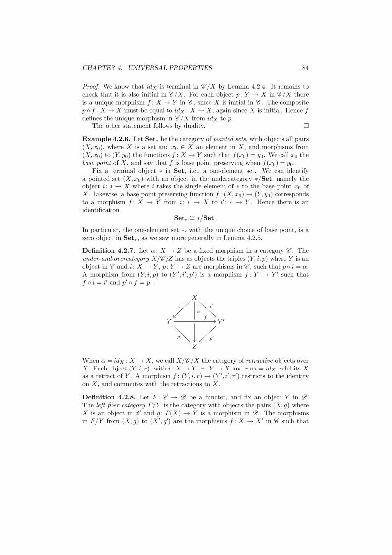
CHAPTER 4. UNIVERSAL PROPERTIES 84
Proof. We know that idX is terminal in C /X by Lemma 4.2.4. It remains tocheck that it is also initial in C /X. For each object p : Y → X in C /X thereis a unique morphism f : X → Y in C , since X is initial in C . The compositep f : X → X must be equal to idX : X → X, again since X is initial. Hence fdefines the unique morphism in C /X from idX to p.
The other statement follows by duality.
Example 4.2.6. Let Set∗ be the category of pointed sets, with objects all pairs(X,x0), where X is a set and x0 ∈ X an element in X, and morphisms from(X,x0) to (Y, y0) the functions f : X → Y such that f(x0) = y0. We call x0 thebase point of X, and say that f is base point preserving when f(x0) = y0.
Fix a terminal object ∗ in Set, i.e., a one-element set. We can identifya pointed set (X,x0) with an object in the undercategory ∗/Set, namely theobject i : ∗ → X where i takes the single element of ∗ to the base point x0 ofX. Likewise, a base point preserving function f : (X,x0) → (Y, y0) correspondsto a morphism f : X → Y from i : ∗ → X to i′ : ∗ → Y . Hence there is anidentification
Set∗ ∼= ∗/Set .
In particular, the one-element set ∗, with the unique choice of base point, is azero object in Set∗, as we saw more generally in Lemma 4.2.5.
Definition 4.2.7. Let α : X → Z be a fixed morphism in a category C . Theunder-and-overcategory X/C /Z has as objects the triples (Y, i, p) where Y is anobject in C and i : X → Y , p : Y → Z are morphisms in C , such that p i = α.A morphism from (Y, i, p) to (Y ′, i′, p′) is a morphism f : Y → Y ′ such thatf i = i′ and p′ f = p.
Xi
~~~~~~
~~~~ i′
ÃÃAAA
AAAA
A
α
²²
Yf
//
pÃÃ
@@@@
@@@@
Y ′
p′
~~
Z
When α = idX : X → X, we call X/C /X the category of retractive objects overX. Each object (Y, i, r), with i : X → Y , r : Y → X and r i = idX exhibits Xas a retract of Y . A morphism f : (Y, i, r) → (Y ′, i′, r′) restricts to the identityon X, and commutes with the retractions to X.
Definition 4.2.8. Let F : C → D be a functor, and fix an object Y in D .The left fiber category F/Y is the category with objects the pairs (X, g) whereX is an object in C and g : F (X) → Y is a morphism in D . The morphismsin F/Y from (X, g) to (X ′, g′) are the morphisms f : X → X ′ in C such that
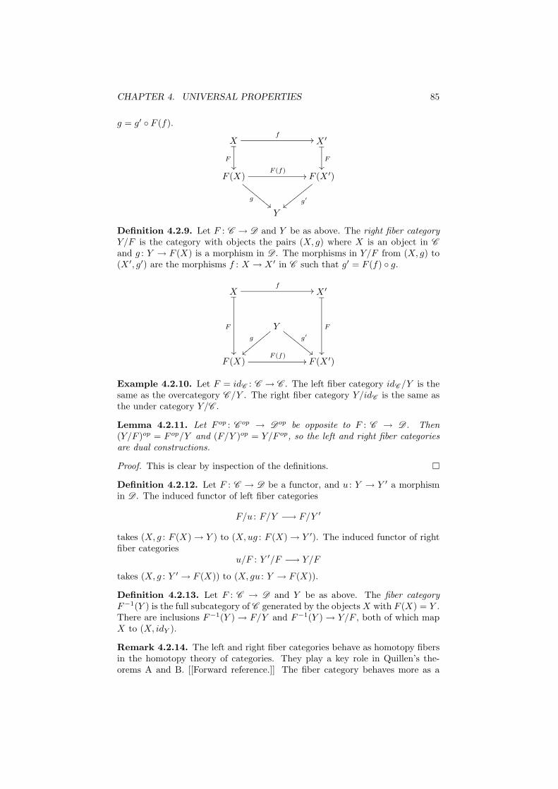
CHAPTER 4. UNIVERSAL PROPERTIES 85
g = g′ F (f).
Xf
//_
F
²²
X ′_
F
²²
F (X)F (f)
//
g""DD
DDDD
DDF (X ′)
g′
||yyyyyyyy
Y
Definition 4.2.9. Let F : C → D and Y be as above. The right fiber categoryY/F is the category with objects the pairs (X, g) where X is an object in C
and g : Y → F (X) is a morphism in D . The morphisms in Y/F from (X, g) to(X ′, g′) are the morphisms f : X → X ′ in C such that g′ = F (f) g.
Xf
//_
F
²²
X ′_
F
²²
Yg
||zzzz
zzzz g′
""EEEEEEEE
F (X)F (f)
// F (X ′)
Example 4.2.10. Let F = idC : C → C . The left fiber category idC /Y is thesame as the overcategory C /Y . The right fiber category Y/idC is the same asthe under category Y/C .
Lemma 4.2.11. Let F op : C op → Dop be opposite to F : C → D . Then(Y/F )op = F op/Y and (F/Y )op = Y/F op, so the left and right fiber categoriesare dual constructions.
Proof. This is clear by inspection of the definitions.
Definition 4.2.12. Let F : C → D be a functor, and u : Y → Y ′ a morphismin D . The induced functor of left fiber categories
F/u : F/Y −→ F/Y ′
takes (X, g : F (X) → Y ) to (X,ug : F (X) → Y ′). The induced functor of rightfiber categories
u/F : Y ′/F −→ Y/F
takes (X, g : Y ′ → F (X)) to (X, gu : Y → F (X)).
Definition 4.2.13. Let F : C → D and Y be as above. The fiber categoryF−1(Y ) is the full subcategory of C generated by the objects X with F (X) = Y .There are inclusions F−1(Y ) → F/Y and F−1(Y ) → Y/F , both of which mapX to (X, idY ).
Remark 4.2.14. The left and right fiber categories behave as homotopy fibersin the homotopy theory of categories. They play a key role in Quillen’s the-orems A and B. [[Forward reference.]] The fiber category behaves more as a
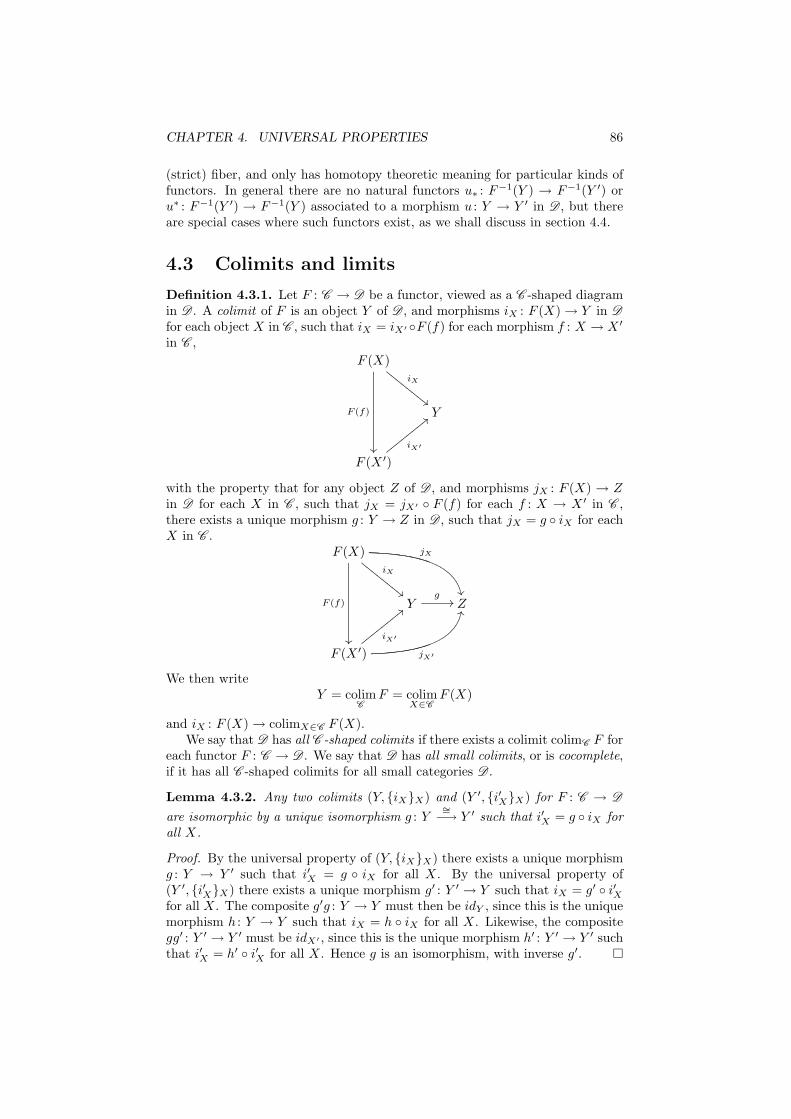
CHAPTER 4. UNIVERSAL PROPERTIES 86
(strict) fiber, and only has homotopy theoretic meaning for particular kinds offunctors. In general there are no natural functors u∗ : F−1(Y ) → F−1(Y ′) oru∗ : F−1(Y ′) → F−1(Y ) associated to a morphism u : Y → Y ′ in D , but thereare special cases where such functors exist, as we shall discuss in section 4.4.
4.3 Colimits and limits
Definition 4.3.1. Let F : C → D be a functor, viewed as a C -shaped diagramin D . A colimit of F is an object Y of D , and morphisms iX : F (X) → Y in D
for each object X in C , such that iX = iX′ F (f) for each morphism f : X → X ′
in C ,
F (X)
F (f)
²²
iX
""EEEEEEEE
Y
F (X ′)
iX′
<<yyyyyyyy
with the property that for any object Z of D , and morphisms jX : F (X) → Zin D for each X in C , such that jX = jX′ F (f) for each f : X → X ′ in C ,there exists a unique morphism g : Y → Z in D , such that jX = g iX for eachX in C .
F (X)
F (f)
²²
iX
""EEEEEEEEjX
µµ
Yg
// Z
F (X ′)
iX′
<<yyyyyyyyjX′
LL
We then writeY = colim
C
F = colimX∈C
F (X)
and iX : F (X) → colimX∈C F (X).We say that D has all C -shaped colimits if there exists a colimit colimC F for
each functor F : C → D . We say that D has all small colimits, or is cocomplete,if it has all C -shaped colimits for all small categories D .
Lemma 4.3.2. Any two colimits (Y, iXX) and (Y ′, i′XX) for F : C → D
are isomorphic by a unique isomorphism g : Y∼=−→ Y ′ such that i′X = g iX for
all X.
Proof. By the universal property of (Y, iXX) there exists a unique morphismg : Y → Y ′ such that i′X = g iX for all X. By the universal property of(Y ′, i′XX) there exists a unique morphism g′ : Y ′ → Y such that iX = g′ i′Xfor all X. The composite g′g : Y → Y must then be idY , since this is the uniquemorphism h : Y → Y such that iX = h iX for all X. Likewise, the compositegg′ : Y ′ → Y ′ must be idX′ , since this is the unique morphism h′ : Y ′ → Y ′ suchthat i′X = h′ i′X for all X. Hence g is an isomorphism, with inverse g′.
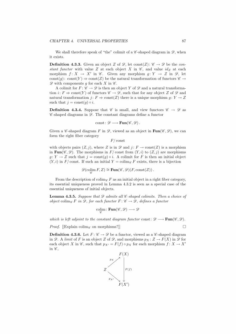
CHAPTER 4. UNIVERSAL PROPERTIES 87
We shall therefore speak of “the” colimit of a C -shaped diagram in D , whenit exists.
Definition 4.3.3. Given an object Z of D , let const(Z) : C → D be the con-stant functor with value Z at each object X in C , and value idZ at eachmorphism f : X → X ′ in C . Given any morphism g : Y → Z in D , letconst(g) : const(Y ) ⇒ const(Z) be the natural transformation of functors C →D with components g for each X in C .
A colimit for F : C → D is then an object Y of D and a natural transforma-tion i : F ⇒ const(Y ) of functors C → D , such that for any object Z of D andnatural transformation j : F ⇒ const(Z) there is a unique morphism g : Y → Zsuch that j = const(g) i.
Definition 4.3.4. Suppose that C is small, and view functors C → D asC -shaped diagrams in D . The constant diagrams define a functor
const : D −→ Fun(C ,D) .
Given a C -shaped diagram F in D , viewed as an object in Fun(C ,D), we canform the right fiber category
F/ const
with objects pairs (Z, j), where Z is in D and j : F → const(Z) is a morphismin Fun(C ,D). The morphisms in F/ const from (Y, i) to (Z, j) are morphismsg : Y → Z such that j = const(g) i. A colimit for F is then an initial object(Y, i) in F/ const. If such an initial Y = colimC F exists, there is a bijection
D(colimC
F,Z) ∼= Fun(C ,D)(F, const(Z)) .
From the description of colimC F as an initial object in a right fiber category,its essential uniqueness proved in Lemma 4.3.2 is seen as a special case of theessential uniqueness of initial objects.
Lemma 4.3.5. Suppose that D admits all C -shaped colimits. Then a choice ofobject colimC F in D , for each functor F : C → D , defines a functor
colimC
: Fun(C ,D) −→ D
which is left adjoint to the constant diagram functor const : D −→ Fun(C ,D).
Proof. [[Explain colimC on morphisms?]]
Definition 4.3.6. Let F : C → D be a functor, viewed as a C -shaped diagramin D . A limit of F is an object Z of D , and morphisms pX : Z → F (X) in D foreach object X in C , such that pX′ = F (f) pX for each morphism f : X → X ′
in C ,
F (X)
F (f)
²²
Z
pX
<<yyyyyyyy
pX′""EEEEEEEE
F (X ′)
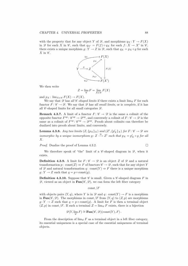
CHAPTER 4. UNIVERSAL PROPERTIES 88
with the property that for any object Y of D , and morphisms qX : Y → F (X)in D for each X in C , such that qX′ = F (f) qX for each f : X → X ′ in C ,there exists a unique morphism g : Y → Z in D , such that qX = pX g for eachX in C .
F (X)
F (f)
²²
Yg
//
qX 00
qX′ ..
Z
pX
<<yyyyyyyy
pX′""EEEEEEEE
F (X ′)
We then writeZ = lim
C
F = limX∈C
F (X)
and pX : limX∈C F (X) → F (X).We say that D has all C -shaped limits if there exists a limit limC F for each
functor F : C → D . We say that D has all small limits, or is complete, if it hasall C -shaped limits for all small categories D .
Remark 4.3.7. A limit of a functor F : C → D is the same a colimit of theopposite functor F op : C op → Dop, and conversely a colimit of F : C → D is thesame as a colimit of F op : C op → Dop. Proofs about colimits can therefore bedualized into proofs about limits, and conversely.
Lemma 4.3.8. Any two limits (Z, pXX) and (Z ′, p′XX) for F : C → D are
isomorphic by a unique isomorphism g : Z∼=−→ Z ′ such that pX = p′X g for all
X.
Proof. Dualize the proof of Lemma 4.3.2.
We therefore speak of “the” limit of a C -shaped diagram in D , when itexists.
Definition 4.3.9. A limit for F : C → D is an object Z of D and a naturaltransformation p : const(Z) ⇒ F of functors C → D , such that for any object Yof D and natural transformation q : const(Y ) ⇒ F there is a unique morphismg : Y → Z such that q = p const(g).
Definition 4.3.10. Suppose that C is small. Given a C -shaped diagram F inD , viewed as an object in Fun(C ,D), we can form the left fiber category
const /F
with objects pairs (Y, q), where Y is in D and q : const(Y ) → F is a morphismin Fun(C ,D). The morphisms in const /F from (Y, q) to (Z, p) are morphismsg : Y → Z such that q = p const(g). A limit for F is then a terminal object(Z, p) in const /F . If such a terminal Z = limC F exists, there is a bijection
D(Y, limC
F ) ∼= Fun(C ,D)(const(Y ), F ) .
From the description of limC F as a terminal object in a left fiber category,its essential uniqueness is a special case of the essential uniqueness of terminalobjects.
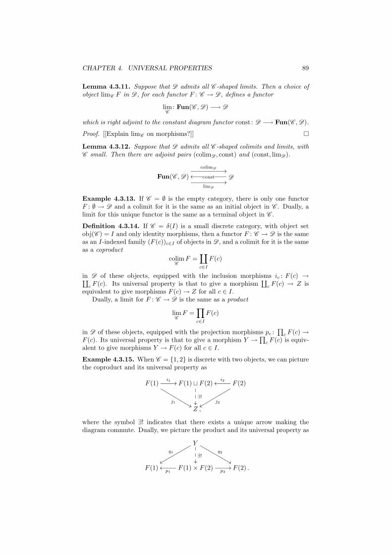
CHAPTER 4. UNIVERSAL PROPERTIES 89
Lemma 4.3.11. Suppose that D admits all C -shaped limits. Then a choice ofobject limC F in D , for each functor F : C → D , defines a functor
limC
: Fun(C ,D) −→ D
which is right adjoint to the constant diagram functor const : D −→ Fun(C ,D).
Proof. [[Explain limC on morphisms?]]
Lemma 4.3.12. Suppose that D admits all C -shaped colimits and limits, withC small. Then there are adjoint pairs (colimD , const) and (const, limD).
Fun(C ,D)
colimD //
limD
//Dconstoo
Example 4.3.13. If C = ∅ is the empty category, there is only one functorF : ∅ → D and a colimit for it is the same as an initial object in C . Dually, alimit for this unique functor is the same as a terminal object in C .
Definition 4.3.14. If C = δ(I) is a small discrete category, with object setobj(C ) = I and only identity morphisms, then a functor F : C → D is the sameas an I-indexed family (F (c))c∈I of objects in D , and a colimit for it is the sameas a coproduct
colimC
F =∐
c∈I
F (c)
in D of these objects, equipped with the inclusion morphisms ic : F (c) →∐c F (c). Its universal property is that to give a morphism
∐c F (c) → Z is
equivalent to give morphisms F (c) → Z for all c ∈ I.Dually, a limit for F : C → D is the same as a product
limC
F =∏
c∈I
F (c)
in D of these objects, equipped with the projection morphisms pc :∏
c F (c) →F (c). Its universal property is that to give a morphism Y →
∏c F (c) is equiv-
alent to give morphisms Y → F (c) for all c ∈ I.
Example 4.3.15. When C = 1, 2 is discrete with two objects, we can picturethe coproduct and its universal property as
F (1)i1 //
j1&&LLLLLLLLLLL
F (1) ⊔ F (2)
∃!
²²ÂÂÂ
F (2)i2oo
j2xxrrrrrrrrrrr
Z ,
where the symbol ∃! indicates that there exists a unique arrow making thediagram commute. Dually, we picture the product and its universal property as
Yq1
xxqqqqqqqqqqq
∃!
²²ÂÂÂ
q2
&&MMMMMMMMMMM
F (1) F (1) × F (2)p1
oop2
// F (2) .
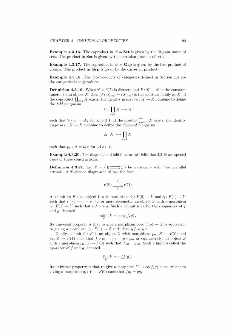
CHAPTER 4. UNIVERSAL PROPERTIES 90
Example 4.3.16. The coproduct in D = Set is given by the disjoint union ofsets. The product in Set is given by the cartesian product of sets.
Example 4.3.17. The coproduct in D = Grp is given by the free product ofgroups. The product in Grp is given by the cartesian product.
Example 4.3.18. The (co-)products of categories defined in Section 1.4 arethe categorical (co-)products.
Definition 4.3.19. When C = δ(I) is discrete and F : C → D is the constantfunctor to an object X, then (F (c))c∈I = (X)c∈I is the constant family at X. Ifthe coproduct
∐c∈I X exists, the identity maps idX : X → X combine to define
the fold morphism
∇ :∐
c∈I
X −→ X
such that ∇ ic = idX for all c ∈ I. If the product∏
c∈I X exists, the identitymaps idX : X → X combine to define the diagonal morphism
∆: X −→∏
c∈I
X
such that pc ∆ = idX for all c ∈ I.
Example 4.3.20. The diagonal and fold functors of Definition 2.3.16 are specialcases of these constructions.
Definition 4.3.21. Let C = 0//// 1 be a category with “two parallel
arrows”. A C -shaped diagram in D has the form
F (0)f
//
g// F (1) .
A colimit for F is an object Y with morphisms i0 : F (0) → Y and i1 : F (1) → Ysuch that i1 f = i0 = i1 g, or more succinctly, an object Y with a morphismi1 : F (1) → Y such that i1f = i1g. Such a colimit is called the coequalizer of fand g, denoted
colimC
F = coeq(f, g) .
Its universal property is that to give a morphism coeq(f, g) → Z is equivalentto giving a morphism j1 : F (1) → Z such that j1f = j1g.
Dually, a limit for F is an object Z with morphisms p0 : Z → F (0) andp1 : Z → F (1) such that f p0 = p1 = g p0, or equivalently, an object Zwith a morphism p0 : Z → F (0) such that fp0 = gp0. Such a limit is called theequalizer of f and g, denoted
limC
F = eq(f, g) .
Its universal property is that to give a morphism Y → eq(f, g) is equivalent togiving a morphism q1 : Y → F (0) such that fq1 = gq1.
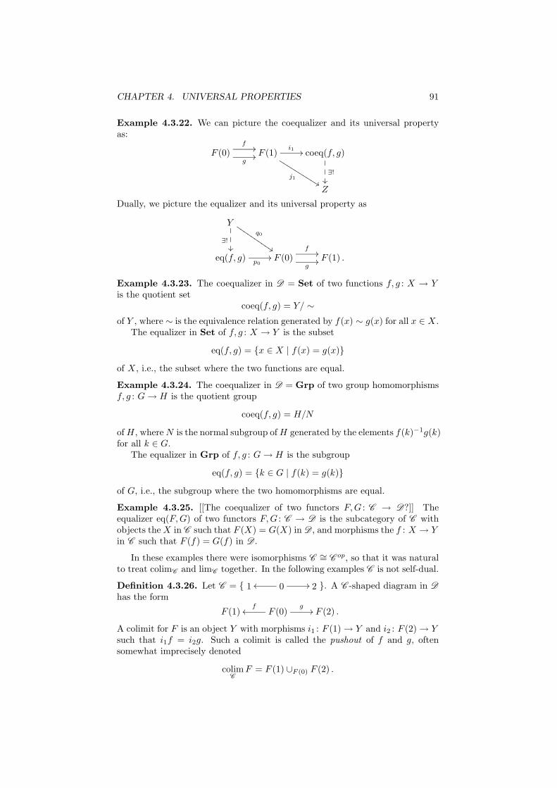
CHAPTER 4. UNIVERSAL PROPERTIES 91
Example 4.3.22. We can picture the coequalizer and its universal propertyas:
F (0)f
//
g// F (1)
i1 //
j1%%KKKKKKKKKK
coeq(f, g)
∃!
²²ÂÂÂ
Z
Dually, we picture the equalizer and its universal property as
Yq0
$$IIII
IIII
II
∃!
²²ÂÂÂ
eq(f, g)p0
// F (0)f
//
g// F (1) .
Example 4.3.23. The coequalizer in D = Set of two functions f, g : X → Yis the quotient set
coeq(f, g) = Y/ ∼
of Y , where ∼ is the equivalence relation generated by f(x) ∼ g(x) for all x ∈ X.The equalizer in Set of f, g : X → Y is the subset
eq(f, g) = x ∈ X | f(x) = g(x)
of X, i.e., the subset where the two functions are equal.
Example 4.3.24. The coequalizer in D = Grp of two group homomorphismsf, g : G → H is the quotient group
coeq(f, g) = H/N
of H, where N is the normal subgroup of H generated by the elements f(k)−1g(k)for all k ∈ G.
The equalizer in Grp of f, g : G → H is the subgroup
eq(f, g) = k ∈ G | f(k) = g(k)
of G, i.e., the subgroup where the two homomorphisms are equal.
Example 4.3.25. [[The coequalizer of two functors F,G : C → D?]] Theequalizer eq(F,G) of two functors F,G : C → D is the subcategory of C withobjects the X in C such that F (X) = G(X) in D , and morphisms the f : X → Yin C such that F (f) = G(f) in D .
In these examples there were isomorphisms C ∼= C op, so that it was naturalto treat colimC and limC together. In the following examples C is not self-dual.
Definition 4.3.26. Let C = 1 0oo // 2 . A C -shaped diagram in D
has the form
F (1) F (0)f
oog
// F (2) .
A colimit for F is an object Y with morphisms i1 : F (1) → Y and i2 : F (2) → Ysuch that i1f = i2g. Such a colimit is called the pushout of f and g, oftensomewhat imprecisely denoted
colimC
F = F (1) ∪F (0) F (2) .
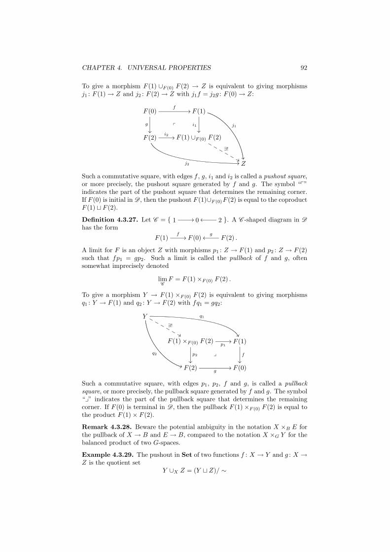
CHAPTER 4. UNIVERSAL PROPERTIES 92
To give a morphism F (1) ∪F (0) F (2) → Z is equivalent to giving morphismsj1 : F (1) → Z and j2 : F (2) → Z with j1f = j2g : F (0) → Z:
F (0)f
//
g
²²
p
F (1)
i1
²²
j1
´´
F (2)i2 //
j2 //
F (1) ∪F (0) F (2)
∃!
&&MMMMMM
Z
Such a commutative square, with edges f , g, i1 and i2 is called a pushout square,or more precisely, the pushout square generated by f and g. The symbol “p”indicates the part of the pushout square that determines the remaining corner.If F (0) is initial in D , then the pushout F (1)∪F (0)F (2) is equal to the coproductF (1) ⊔ F (2).
Definition 4.3.27. Let C = 1 // 0 2oo . A C -shaped diagram in D
has the form
F (1)f
// F (0) F (2) .g
oo
A limit for F is an object Z with morphisms p1 : Z → F (1) and p2 : Z → F (2)such that fp1 = gp2. Such a limit is called the pullback of f and g, oftensomewhat imprecisely denoted
limC
F = F (1) ×F (0) F (2) .
To give a morphism Y → F (1) ×F (0) F (2) is equivalent to giving morphismsq1 : Y → F (1) and q2 : Y → F (2) with fq1 = gq2:
Y q1
ºº
q2
**
∃!
&&MMMMMM
F (1) ×F (0) F (2)p1
//
p2
²²
y
F (1)
f
²²
F (2)g
// F (0)
Such a commutative square, with edges p1, p2, f and g, is called a pullbacksquare, or more precisely, the pullback square generated by f and g. The symbol“y” indicates the part of the pullback square that determines the remainingcorner. If F (0) is terminal in D , then the pullback F (1) ×F (0) F (2) is equal tothe product F (1) × F (2).
Remark 4.3.28. Beware the potential ambiguity in the notation X ×B E forthe pullback of X → B and E → B, compared to the notation X ×G Y for thebalanced product of two G-spaces.
Example 4.3.29. The pushout in Set of two functions f : X → Y and g : X →Z is the quotient set
Y ∪X Z = (Y ⊔ Z)/ ∼
CHAPTER 4. UNIVERSAL PROPERTIES 93
where ∼ is the equivalence relation generated by the identification of f(x) ∈Y ⊆ Y ⊔ Z with g(x) ∈ Z ⊆ Y ⊔ Z, for all x ∈ X. If f : X → Y is injective,then the inclusion Z → Y ∪X Z is injective, and each element in Y ∪X Z canbe uniquely expressed either as an element in Y \ f(X), or as an element in Z.
The pullback in Set of two functions f : X → Z and g : Y → Z is the subset
X ×Z Y = (x, y) ∈ X × Y | f(x) = g(y) ,
also known as the fiber product of X and Y over Z. For each x ∈ X the fiber ofX ×Z Y over x, meaning the preimage of x under the projection X ×Z Y → X,can be identified with the fiber g−1(f(x)) of Y over f(x), meaning the preimageof f(x) under the function g : Y → Z.
Example 4.3.30. The pushout in Grp of two homomorphisms f : K → H andg : K → G is the amalgamated free product
colimHf← K
g→ G = H ∗K G
obtained as the quotient group of the free product H∗K by the normal subgroupgenerated by the words f(k)−1g(k) for all k ∈ K.
The pullback in Grp of two homomorphisms f : H → G and g : K → G isthe subgroup
H ×G K = (h, k) ∈ H × K | f(h) = g(k) ,
of the direct product H × G.
[[Pushout and pullback in Cat.]]
Definition 4.3.31. Let C be a category with a terminal object ∗. A cofiber ofa morphism f : X → Y is a pushout of the diagram
∗ ←− X −→ Y .
We write Y/X or Y/f(X) for this pushout ∗ ∪X Y . There are preferred mor-phisms ∗ → Y/X ← Y .
Given a morphism p : ∗ → Y , the fiber of a morphism f : X → Y at p is apullback of the diagram
∗p
−→ Xf
←− X .
We write f−1(p) for this pullback. There is a preferred morphism f−1(p) → X.
Example 4.3.32. In sSet, the cofiber of a function f : X → Y is the quotientset Y/f(X) = (Y ⊔ ∗)/ ∼, where f(x) ∼ ∗ for each x ∈ X. Note thatY/∅ = Y+ = Y ⊔ ∗. A morphism ∗ → Y corresponds to a point p ∈ Y , andthe fiber of f : X → Y at p is the subset f−1(p) = x ∈ X | f(x) = p.
[[Sequential colimit, sequential limit.]][[Also discuss finite categories, with finitely many morphisms, and finite col-
imits? Beware that the nerve of a finite category needs not be a finite simplicialset.]]
Lemma 4.3.33. Suppose that D has all small coproducts and coequalizers.Then D has all small colimits.
Dually, suppose that D has all small products and equalizers. Then D hasall small limits.
CHAPTER 4. UNIVERSAL PROPERTIES 94
Proof. The colimit of F : C → D is given by the coequalizer of the two mor-phisms
s, t :∐
f : X→Y
F (X) −→∐
X
F (X)
where f ranges over all morphisms in C and X ranges over all objects in C .The morphism s is determined by its restrictions s if = iX for f : X → Y ,while the morphism t is determined by its restrictions t if = iY F (f).
Dually, the limit of F : C → D is given by the equalizer of the two morphisms
s, t :∏
X
F (X) −→∏
f : X→Y
F (X)
where X ranges over all objects in C and f ranges over all morphisms in C . Themorphism s is determined by its projections pf s = F (f) pX for f : X → Y ,while the morphism t is determined by its projections pf t = pY .
[[What remains to be verified?]]
Example 4.3.34. The colimit of a C -shaped diagram in sets, X : C → Set, isthe quotient set
colimC
X =∐
c
X(c)/∼
where ∼ is generated by ic(x) ∼ id(X(a)(x)) for all a : c → d and x ∈ X(c), ormore concisely, X(c) ∋ x ∼ a∗(x) ∈ X(d).
Dually, its limit is the subset
limC
X ⊆∏
c
X(c)
of sequences (xc)c with xc ∈ X(c) for all c in C , such that X(a)(xc) = xd forall a : c → d, or more briefly, a∗(xc) = xd.
Lemma 4.3.35. Let F : C → D have colimit colimC F and let Z be an objectof D . There is a natural bijection
D(colimC
F,Z) ∼= limX∈C
D(F (X), Z) .
Dually, let G : C → D have limit limC G and let Z be an object of D . There isa natural bijection
D(Z, limC
G) ∼= limX∈C
D(Z,G(X)) .
Proof. The first two sets are both identified with the families (φX)X of mor-phisms φX : F (X) → Z in D for all X in C , with φY F (f) = φX for allf : X → Y in C .
The last two sets are both identified with the families (ψX)X of morphismsψX : Z → G(X) in D for all X in C , with G(f) ψX = ψY for all f : X → Y inC .
The following is a useful tool for checking that a functor respects (co-)limits,or for showing that is cannot be a (co-)adjoint.
CHAPTER 4. UNIVERSAL PROPERTIES 95
Proposition 4.3.36. Let F : C → D and G : D → C be an adjoint pair, andlet E be a small category. If X : E → C is an E -shaped diagram in C , withcolimit colimE X, then F X : E → D has the colimit
colimE
(F X) = F (colimE
X) .
Dually, if Y : E → D is an E -shaped diagram in D , with limit limE Y , thenG Y : E → C has the limit
limE
(G Y ) = G(limE
Y ) .
In other words, a left adjoint (= coadjoint) preserves colimits, and a right ad-joint (= adjoint) preserves limits.
Proof. For any object Y in D there are natural bijections
D(F (colimE
X), Y ) ∼= C (colimE
X,G(Y ))
∼= limE
C (X(−), G(Y ))
∼= limE
D(F (X(−)), Y )
∼= Fun(E ,D)(F X, const(Y ))
which show that F (colimE X) is a colimit of F X.Dually, for any object X in C there are natural bijections
C (X,G(limE
Y )) ∼= D(F (X), limE
Y )
∼= limE
D(F (X), Y (−))
∼= limE
C (X,G(Y (−)))
∼= Fun(E ,C )(const(X), G Y )
which show that G(limE Y ) is a limit of G Y .
Lemma 4.3.37. Suppose that C has a terminal object Z. Then each functorF : C → D has a colimit
colimC
F = F (Z)
given by the object F (Z) and the structure morphism iX = F (X → Z) : F (X) →F (Z) for all X in C .
Lemma 4.3.38. Suppose that C has an initial object Y . Then each functorF : C → D has a limit
limC
F = F (Y )
given by the object F (Y ) and the structure morphism pX = F (Y → X) : F (Y ) →F (X) for all X in C .
[[Filtering (co-)limits?]]
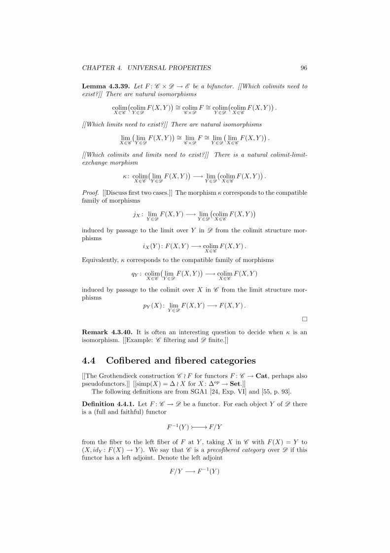
CHAPTER 4. UNIVERSAL PROPERTIES 96
Lemma 4.3.39. Let F : C × D → E be a bifunctor. [[Which colimits need toexist?]] There are natural isomorphisms
colimX∈C
(colimY ∈D
F (X,Y ))∼= colim
C×D
F ∼= colimY ∈D
(colimX∈C
F (X,Y )).
[[Which limits need to exist?]] There are natural isomorphisms
limX∈C
(limY ∈D
F (X,Y ))∼= lim
C×D
F ∼= limY ∈D
(lim
X∈C
F (X,Y )).
[[Which colimits and limits need to exist?]] There is a natural colimit-limit-exchange morphism
κ : colimX∈C
(limY ∈D
F (X,Y ))−→ lim
Y ∈D
(colimX∈C
F (X,Y )).
Proof. [[Discuss first two cases.]] The morphism κ corresponds to the compatiblefamily of morphisms
jX : limY ∈D
F (X,Y ) −→ limY ∈D
(colimX∈C
F (X,Y ))
induced by passage to the limit over Y in D from the colimit structure mor-phisms
iX(Y ) : F (X,Y ) −→ colimX∈C
F (X,Y ) .
Equivalently, κ corresponds to the compatible family of morphisms
qY : colimX∈C
(limY ∈D
F (X,Y ))−→ colim
X∈C
F (X,Y )
induced by passage to the colimit over X in C from the limit structure mor-phisms
pY (X) : limY ∈D
F (X,Y ) −→ F (X,Y ) .
Remark 4.3.40. It is often an interesting question to decide when κ is anisomorphism. [[Example: C filtering and D finite.]]
4.4 Cofibered and fibered categories
[[The Grothendieck construction C ≀ F for functors F : C → Cat, perhaps alsopseudofunctors.]] [[simp(X) = ∆ ≀ X for X : ∆op → Set.]]
The following definitions are from SGA1 [24, Exp. VI] and [55, p. 93].
Definition 4.4.1. Let F : C → D be a functor. For each object Y of D thereis a (full and faithful) functor
F−1(Y ) // // F/Y
from the fiber to the left fiber of F at Y , taking X in C with F (X) = Y to(X, idY : F (X) → Y ). We say that C is a precofibered category over D if thisfunctor has a left adjoint. Denote the left adjoint
F/Y −→ F−1(Y )
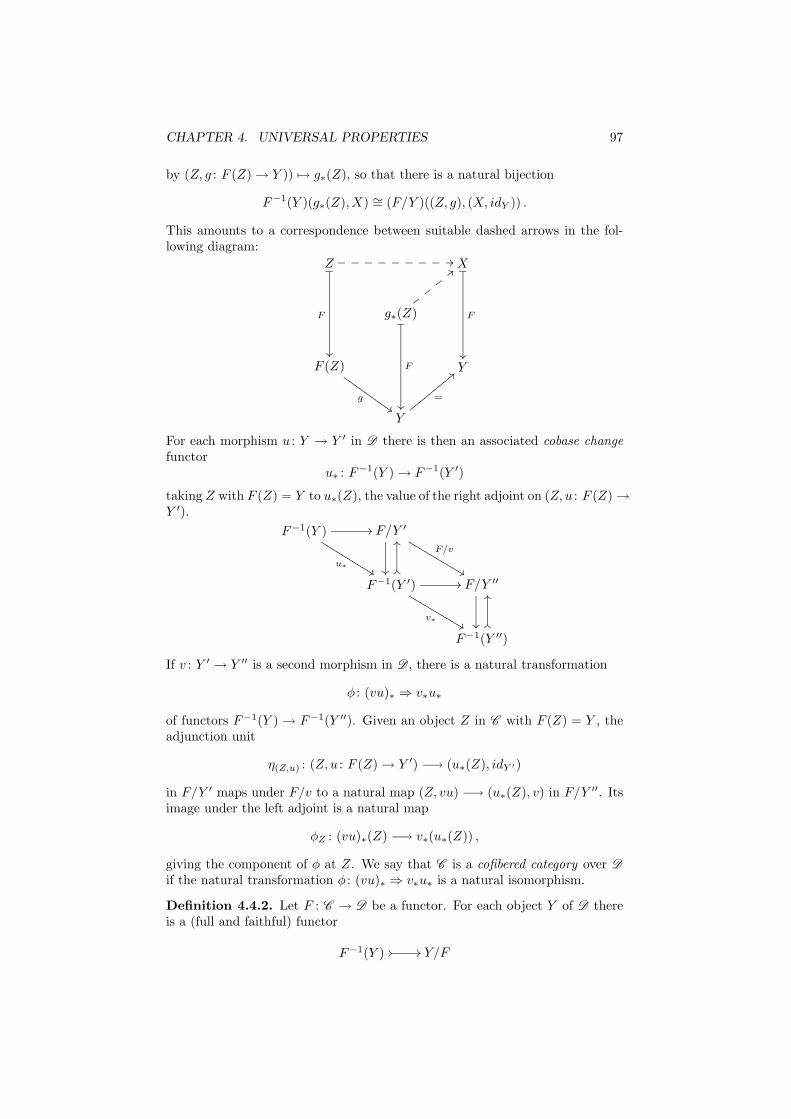
CHAPTER 4. UNIVERSAL PROPERTIES 97
by (Z, g : F (Z) → Y )) 7→ g∗(Z), so that there is a natural bijection
F−1(Y )(g∗(Z),X) ∼= (F/Y )((Z, g), (X, idY )) .
This amounts to a correspondence between suitable dashed arrows in the fol-lowing diagram:
Z //__________
F
²²
X_
F
²²
g∗(Z)
<<yy
yy
_
F
²²
F (Z)
g$$HHHHHHHHH Y
Y
=
<<yyyyyyyyy
For each morphism u : Y → Y ′ in D there is then an associated cobase changefunctor
u∗ : F−1(Y ) → F−1(Y ′)
taking Z with F (Z) = Y to u∗(Z), the value of the right adjoint on (Z, u : F (Z) →Y ′).
F−1(Y ) //
u∗%%KKKKKKKKKKF/Y ′
²²
F/v
%%LLLLLLLLLL
F−1(Y ′) //
v∗%%LLLLLLLLLL
OO
OO
F/Y ′′
²²
F−1(Y ′′)
OO
OO
If v : Y ′ → Y ′′ is a second morphism in D , there is a natural transformation
φ : (vu)∗ ⇒ v∗u∗
of functors F−1(Y ) → F−1(Y ′′). Given an object Z in C with F (Z) = Y , theadjunction unit
η(Z,u) : (Z, u : F (Z) → Y ′) −→ (u∗(Z), idY ′)
in F/Y ′ maps under F/v to a natural map (Z, vu) −→ (u∗(Z), v) in F/Y ′′. Itsimage under the left adjoint is a natural map
φZ : (vu)∗(Z) −→ v∗(u∗(Z)) ,
giving the component of φ at Z. We say that C is a cofibered category over D
if the natural transformation φ : (vu)∗ ⇒ v∗u∗ is a natural isomorphism.
Definition 4.4.2. Let F : C → D be a functor. For each object Y of D thereis a (full and faithful) functor
F−1(Y ) // // Y/F
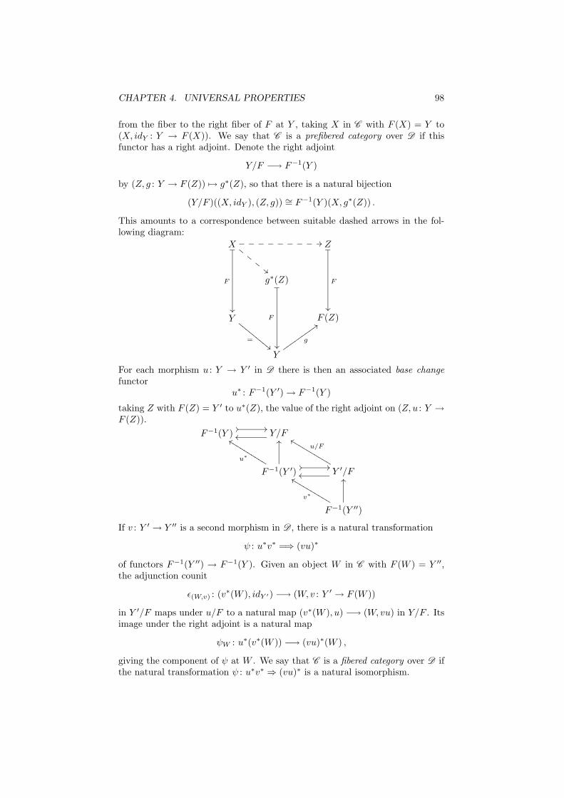
CHAPTER 4. UNIVERSAL PROPERTIES 98
from the fiber to the right fiber of F at Y , taking X in C with F (X) = Y to(X, idY : Y → F (X)). We say that C is a prefibered category over D if thisfunctor has a right adjoint. Denote the right adjoint
Y/F −→ F−1(Y )
by (Z, g : Y → F (Z)) 7→ g∗(Z), so that there is a natural bijection
(Y/F )((X, idY ), (Z, g)) ∼= F−1(Y )(X, g∗(Z)) .
This amounts to a correspondence between suitable dashed arrows in the fol-lowing diagram:
X
""EE
EE
//__________
F
²²
Z_
F
²²
g∗(Z)_
F
²²
Y
=""EE
EEEE
EEE F (Z)
Y
g
::vvvvvvvvv
For each morphism u : Y → Y ′ in D there is then an associated base changefunctor
u∗ : F−1(Y ′) → F−1(Y )
taking Z with F (Z) = Y ′ to u∗(Z), the value of the right adjoint on (Z, u : Y →F (Z)).
F−1(Y )// //
Y/Foo
F−1(Y ′)
OO
u∗
eeKKKKKKKKKK// //
Y ′/Foo
u/FeeLLLLLLLLLL
F−1(Y ′′)
OO
v∗
eeLLLLLLLLLL
If v : Y ′ → Y ′′ is a second morphism in D , there is a natural transformation
ψ : u∗v∗ =⇒ (vu)∗
of functors F−1(Y ′′) → F−1(Y ). Given an object W in C with F (W ) = Y ′′,the adjunction counit
ǫ(W,v) : (v∗(W ), idY ′) −→ (W, v : Y ′ → F (W ))
in Y ′/F maps under u/F to a natural map (v∗(W ), u) −→ (W, vu) in Y/F . Itsimage under the right adjoint is a natural map
ψW : u∗(v∗(W )) −→ (vu)∗(W ) ,
giving the component of ψ at W . We say that C is a fibered category over D ifthe natural transformation ψ : u∗v∗ ⇒ (vu)∗ is a natural isomorphism.
Chapter 5
Homotopy theory
[[Topological spaces Top, CW complexes, compactly generated spaces U . Com-pare Hatcher [26, App. A], May [43, Ch. 5] and McCord [45, §2]. Kelleyfication.]]
[[NOTE: Revise discussion of gluing lemma, following [26, 4.G].]]
5.1 Topological spaces
Recall that Top denotes the category of topological spaces X and continuousfunctions f : X → Y , also known as maps.
Definition 5.1.1. Let Top∗ be the category of based topological spaces (X,x0),with x0 ∈ X, and base point preserving maps (= based maps) f : (X,x0) →(Y, y0), which are maps f : X → Y with f(x0) = y0. When the choice of basepoint is clear, we often simply write X for (X,x0).
Remark 5.1.2. Let ∗ be a fixed one-point space, a terminal object in Top.Each point x0 ∈ X determines a unique map ∗ → X, taking the point in ∗ tox0, and conversely, so there is an isomorphism of categories Top∗
∼= ∗/Top.Here ∗/Top denotes the undercategory of ∗ in Top, as in Definition 4.2.1.
Definition 5.1.3. Let Y be a topological space. A subset X of Y can be giventhe subspace topology, which is the coarsest topology making the inclusion mapi : X → Y continuous. Hence a subset of X is open if and only if it is of the formX ∩U for U open in Y . We then say that X is a subspace of Y . If x0 ∈ X then(X,x0) is a based subspace of (Y, x0). A map i : X → Y is called an embedding(or an inclusion) if it induces a homeomorphism of X with the subspace i(X)of Y .
Definition 5.1.4. Let ∼ be an equivalence relation on a topological space X.The quotient set X/∼ of X can be given the quotient topology, which is the finesttopology making the projection map p : X → X/∼ continuous. Hence a subsetU of X/∼ is open if and only if the preimage p−1(U) is open in X. We thensay that X/∼ is a quotient space of X. If X is based at x0 then (X/∼, p(x0)) isa based quotient space of X. A map p : X → Y is called an identification (or aproclusion) if it induces a homeomorphism of the quotient space X/∼ with Y ,where x ∼ y if and only if p(x) = p(y).
99
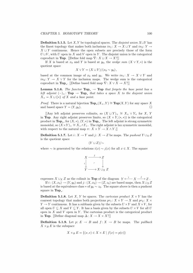
CHAPTER 5. HOMOTOPY THEORY 100
Definition 5.1.5. Let X,Y be topological spaces. The disjoint union X⊔Y hasthe finest topology that makes both inclusions in1 : X → X ⊔ Y and in2 : Y →X ⊔ Y continuous. Hence the open subsets are precisely those of the formU ⊔V , with U open in X and V open in Y . The disjoint union is the categoricalcoproduct in Top. [[Define fold map ∇ : X ⊔ X → X?]]
If X is based at x0 and Y is based at y0, the wedge sum (X ∨ Y, ∗) is thequotient space
X ∨ Y = (X ⊔ Y )/(x0 ∼ y0) ,
based at the common image of x0 and y0. We write in1 : X → X ∨ Y andin2 : Y → X ∨ Y for the inclusion maps. The wedge sum is the categoricalcoproduct in Top∗. [[Define based fold map ∇ : X ∨ X → X?]]
Lemma 5.1.6. The functor Top∗ → Top that forgets the base point has aleft adjoint (−)+ : Top → Top∗ that takes a space X to the disjoint unionX+ = X ⊔ ∗ of X and a base point.
Proof. There is a natural bijection Top∗(X+, Y ) ∼= Top(X,Y ) for any space Xand based space Y = (Y, y0).
[[Any left adjoint preserves colimits, so (X ⊔ Y )+ ∼= X+ ∨ Y+ for X, Yin Top. Any right adjoint preserves limits, so (X × Y, (∗, ∗)) is the categoricalproduct in Top∗, for (X, ∗), (Y, ∗) in Top∗. The left adjoint is strong symmetricmonoidal, so (X×Y )+ ∼= X+∧Y+. The right adjoint is lax symmetric monoidal,with respect to the natural map π : X × Y → X ∧ Y .]]
Definition 5.1.7. Let i : X → Y and j : X → Z be maps. The pushout Y ∪X Zis the quotient space
(Y ⊔ Z)/∼
where ∼ is generated by the relations i(x) ∼ j(x) for all x ∈ X. The square
Xj
//
i
²²
p
Z
²²
Y // X ∪X Z
expresses X ∪X Z as the colimit in Top of the diagram Y Xioo
j// Z .
If i : (X,x0) → (Y, y0) and j : (X,x0) → (Z, z0) are based maps, then X∪X Zis based at the equivalence class ∗ of y0 ∼ z0. The square above is then a pushoutsquare in Top∗.
Definition 5.1.8. Let X, Y be spaces. The cartesian product X × Y has thecoarsest topology that makes both projections pr1 : X × Y → X and pr2 : X ×Y → Y continuous. It has a subbasis given by the subsets U ×Y and X×V , forall open U ⊆ X and V ⊆ Y . It has a basis given by the subsets U ×V for all Uopen in X and V open in Y . The cartesian product is the categorical productin Top. [[Define diagonal map ∆: X → X × X?]]
Definition 5.1.9. Let p : E → B and f : X → B be maps. The pullbackX ×B E is the subspace
X ×B E = (x, e) ∈ X × E | f(x) = p(e)
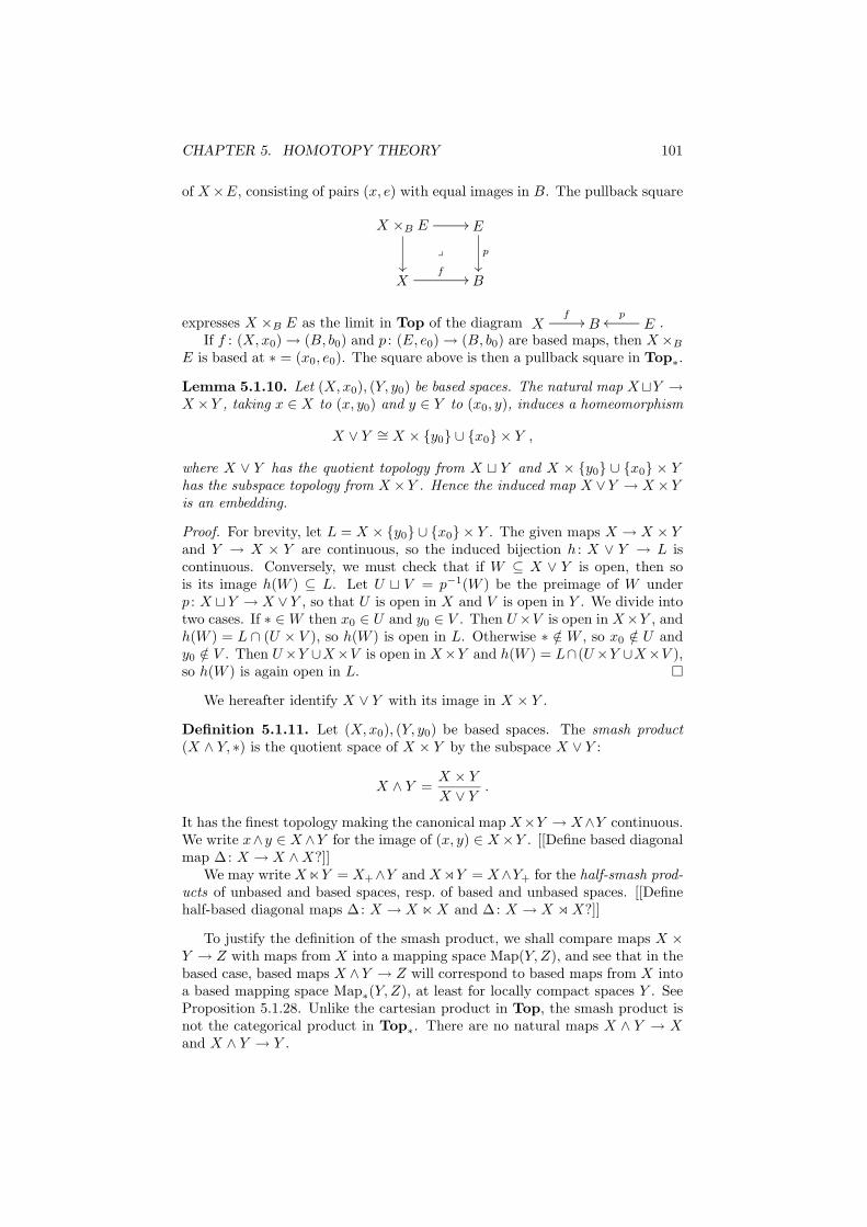
CHAPTER 5. HOMOTOPY THEORY 101
of X×E, consisting of pairs (x, e) with equal images in B. The pullback square
X ×B E //
²²
y
E
p
²²
Xf
// B
expresses X ×B E as the limit in Top of the diagram Xf
// B Ep
oo .If f : (X,x0) → (B, b0) and p : (E, e0) → (B, b0) are based maps, then X ×B
E is based at ∗ = (x0, e0). The square above is then a pullback square in Top∗.
Lemma 5.1.10. Let (X,x0), (Y, y0) be based spaces. The natural map X⊔Y →X ×Y , taking x ∈ X to (x, y0) and y ∈ Y to (x0, y), induces a homeomorphism
X ∨ Y ∼= X × y0 ∪ x0 × Y ,
where X ∨ Y has the quotient topology from X ⊔ Y and X × y0 ∪ x0 × Yhas the subspace topology from X ×Y . Hence the induced map X ∨Y → X ×Yis an embedding.
Proof. For brevity, let L = X × y0 ∪ x0 × Y . The given maps X → X × Yand Y → X × Y are continuous, so the induced bijection h : X ∨ Y → L iscontinuous. Conversely, we must check that if W ⊆ X ∨ Y is open, then sois its image h(W ) ⊆ L. Let U ⊔ V = p−1(W ) be the preimage of W underp : X ⊔ Y → X ∨ Y , so that U is open in X and V is open in Y . We divide intotwo cases. If ∗ ∈ W then x0 ∈ U and y0 ∈ V . Then U ×V is open in X×Y , andh(W ) = L ∩ (U × V ), so h(W ) is open in L. Otherwise ∗ /∈ W , so x0 /∈ U andy0 /∈ V . Then U ×Y ∪X×V is open in X×Y and h(W ) = L∩(U ×Y ∪X×V ),so h(W ) is again open in L.
We hereafter identify X ∨ Y with its image in X × Y .
Definition 5.1.11. Let (X,x0), (Y, y0) be based spaces. The smash product(X ∧ Y, ∗) is the quotient space of X × Y by the subspace X ∨ Y :
X ∧ Y =X × Y
X ∨ Y.
It has the finest topology making the canonical map X×Y → X∧Y continuous.We write x∧y ∈ X ∧Y for the image of (x, y) ∈ X ×Y . [[Define based diagonalmap ∆: X → X ∧ X?]]
We may write X ⋉Y = X+∧Y and X ⋊Y = X∧Y+ for the half-smash prod-ucts of unbased and based spaces, resp. of based and unbased spaces. [[Definehalf-based diagonal maps ∆: X → X ⋉ X and ∆: X → X ⋊ X?]]
To justify the definition of the smash product, we shall compare maps X ×Y → Z with maps from X into a mapping space Map(Y,Z), and see that in thebased case, based maps X ∧Y → Z will correspond to based maps from X intoa based mapping space Map∗(Y,Z), at least for locally compact spaces Y . SeeProposition 5.1.28. Unlike the cartesian product in Top, the smash product isnot the categorical product in Top∗. There are no natural maps X ∧ Y → Xand X ∧ Y → Y .
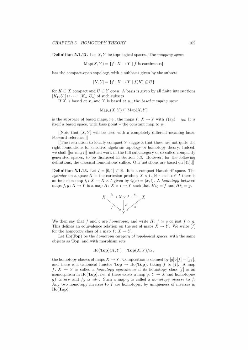
CHAPTER 5. HOMOTOPY THEORY 102
Definition 5.1.12. Let X,Y be topological spaces. The mapping space
Map(X,Y ) = f : X → Y | f is continuous
has the compact-open topology, with a subbasis given by the subsets
[K,U ] = f : X → Y | f(K) ⊆ U
for K ⊆ X compact and U ⊆ Y open. A basis is given by all finite intersections[K1, U1] ∩ · · · ∩ [Kn, Un] of such subsets.
If X is based at x0 and Y is based at y0, the based mapping space
Map∗(X,Y ) ⊆ Map(X,Y )
is the subspace of based maps, i.e., the maps f : X → Y with f(x0) = y0. It isitself a based space, with base point ∗ the constant map to y0.
[[Note that [X,Y ] will be used with a completely different meaning later.Forward reference.]]
[[The restriction to locally compact Y suggests that these are not quite theright foundations for effective algebraic topology or homotopy theory. Indeed,we shall [[or may?]] instead work in the full subcategory of so-called compactlygenerated spaces, to be discussed in Section 5.3. However, for the followingdefinitions, the classical foundations suffice. Our notations are based on [43].]]
Definition 5.1.13. Let I = [0, 1] ⊂ R. It is a compact Hausdorff space. Thecylinder on a space X is the cartesian product X × I. For each t ∈ I there isan inclusion map it : X → X × I given by it(x) = (x, t). A homotopy betweenmaps f, g : X → Y is a map H : X × I → Y such that Hi0 = f and Hi1 = g.
Xi0 //
f##FF
FFFF
FFF X × I
H
²²
Xi1oo
gxx
xxxx
xxx
Y
We then say that f and g are homotopic, and write H : f ≃ g or just f ≃ g.This defines an equivalence relation on the set of maps X → Y . We write [f ]for the homotopy class of a map f : X → Y .
Let Ho(Top) be the homotopy category of topological spaces, with the sameobjects as Top, and with morphism sets
Ho(Top)(X,Y ) = Top(X,Y )/≃ ,
the homotopy classes of maps X → Y . Composition is defined by [g][f ] = [gf ],and there is a canonical functor Top → Ho(Top), taking f to [f ]. A mapf : X → Y is called a homotopy equivalence if its homotopy class [f ] is anisomorphism in Ho(Top), i.e., if there exists a map g : Y → X and homotopiesgf ≃ idX and fg ≃ idY . Such a map g is called a homotopy inverse to f .Any two homotopy inverses to f are homotopic, by uniqueness of inverses inHo(Top).
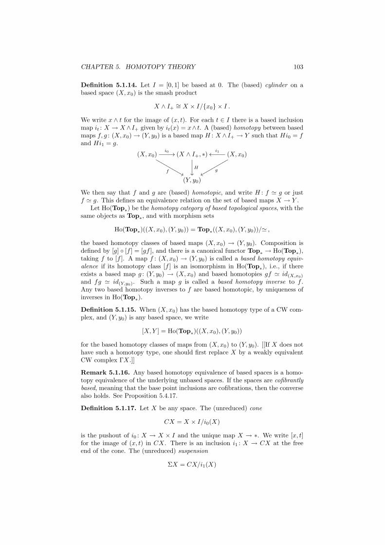
CHAPTER 5. HOMOTOPY THEORY 103
Definition 5.1.14. Let I = [0, 1] be based at 0. The (based) cylinder on abased space (X,x0) is the smash product
X ∧ I+∼= X × I/x0 × I .
We write x ∧ t for the image of (x, t). For each t ∈ I there is a based inclusionmap it : X → X ∧I+ given by it(x) = x∧ t. A (based) homotopy between basedmaps f, g : (X,x0) → (Y, y0) is a based map H : X ∧ I+ → Y such that Hi0 = fand Hi1 = g.
(X,x0)i0 //
f&&MMMMMMMMMM
(X ∧ I+, ∗)
H
²²
(X,x0)i1oo
gxxqqqqqqqqqq
(Y, y0)
We then say that f and g are (based) homotopic, and write H : f ≃ g or justf ≃ g. This defines an equivalence relation on the set of based maps X → Y .
Let Ho(Top∗) be the homotopy category of based topological spaces, with thesame objects as Top∗, and with morphism sets
Ho(Top∗)((X,x0), (Y, y0)) = Top∗((X,x0), (Y, y0))/≃ ,
the based homotopy classes of based maps (X,x0) → (Y, y0). Composition isdefined by [g] [f ] = [gf ], and there is a canonical functor Top∗ → Ho(Top∗),taking f to [f ]. A map f : (X,x0) → (Y, y0) is called a based homotopy equiv-alence if its homotopy class [f ] is an isomorphism in Ho(Top∗), i.e., if thereexists a based map g : (Y, y0) → (X,x0) and based homotopies gf ≃ id(X,x0)
and fg ≃ id(Y,y0). Such a map g is called a based homotopy inverse to f .Any two based homotopy inverses to f are based homotopic, by uniqueness ofinverses in Ho(Top∗).
Definition 5.1.15. When (X,x0) has the based homotopy type of a CW com-plex, and (Y, y0) is any based space, we write
[X,Y ] = Ho(Top∗)((X,x0), (Y, y0))
for the based homotopy classes of maps from (X,x0) to (Y, y0). [[If X does nothave such a homotopy type, one should first replace X by a weakly equivalentCW complex ΓX.]]
Remark 5.1.16. Any based homotopy equivalence of based spaces is a homo-topy equivalence of the underlying unbased spaces. If the spaces are cofibrantlybased, meaning that the base point inclusions are cofibrations, then the conversealso holds. See Proposition 5.4.17.
Definition 5.1.17. Let X be any space. The (unreduced) cone
CX = X × I/i0(X)
is the pushout of i0 : X → X × I and the unique map X → ∗. We write [x, t]for the image of (x, t) in CX. There is an inclusion i1 : X → CX at the freeend of the cone. The (unreduced) suspension
ΣX = CX/i1(X)
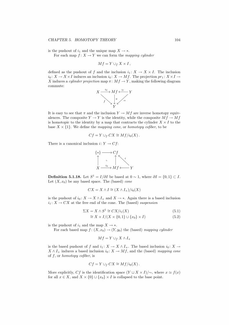
CHAPTER 5. HOMOTOPY THEORY 104
is the pushout of i1 and the unique map X → ∗.For each map f : X → Y we can form the mapping cylinder
Mf = Y ∪f X × I ,
defined as the pushout of f and the inclusion i1 : X → X × I. The inclusioni0 : X → X×I induces an inclusion i0 : X → Mf . The projection pr1 : X×I →X induces a cylinder projection map π : Mf → Y , making the following diagramcommute:
Xi0 //
f!!CC
CCCC
CCMf
π
²²
Y≃oo
=||
||||
||
Y
It is easy to see that π and the inclusion Y → Mf are inverse homotopy equiv-alences. The composite Y → Y is the identity, while the composite Mf → Mfis homotopic to the identity by a map that contracts the cylinder X × I to thebase X × 1. We define the mapping cone, or homotopy cofiber, to be
Cf = Y ∪f CX ∼= Mf/i0(X) .
There is a canonical inclusion i : Y → Cf :
∗ // Cf
X
OO
i0 //
x
Mf
OO
Y
i
``AAAAAAAAoo
Definition 5.1.18. Let S1 = I/∂I be based at 0 ∼ 1, where ∂I = 0, 1 ⊂ I.Let (X,x0) be any based space. The (based) cone
CX = X ∧ I ∼= (X ∧ I+)/i0(X)
is the pushout of i0 : X → X ∧ I+ and X → ∗. Again there is a based inclusioni1 : X → CX at the free end of the cone. The (based) suspension
ΣX = X ∧ S1 ∼= CX/i1(X) (5.1)∼= X × I/(X × 0, 1 ∪ x0 × I) (5.2)
is the pushout of i1 and the map X → ∗.For each based map f : (X,x0) → (Y, y0) the (based) mapping cylinder
Mf = Y ∪f X ∧ I+
is the based pushout of f and i1 : X → X ∧ I+. The based inclusion i0 : X →X ∧ I+ induces a based inclusion i0 : X → Mf , and the (based) mapping coneof f , or homotopy cofiber, is
Cf = Y ∪f CX ∼= Mf/i0(X) .
More explicitly, Cf is the identification space (Y ⊔ X × I)/∼, where x ≃ f(x)for all x ∈ X, and X × 0 ∪ x0 × I is collapsed to the base point.
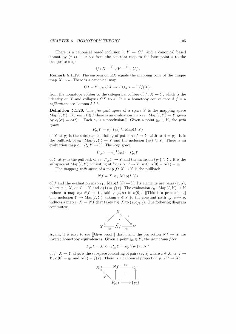
CHAPTER 5. HOMOTOPY THEORY 105
There is a canonical based inclusion i : Y → Cf , and a canonical basedhomotopy (x, t) 7→ x ∧ t from the constant map to the base point ∗ to thecomposite map
if : Xf
// Yi // Cf .
Remark 5.1.19. The suspension ΣX equals the mapping cone of the uniquemap X → ∗. There is a canonical map
Cf = Y ∪X CX → Y ∪X ∗ = Y/f(X) ,
from the homotopy cofiber to the categorical cofiber of f : X → Y , which is theidentity on Y and collapses CX to ∗. It is a homotopy equivalence if f is acofibration, see Lemma 5.5.3.
Definition 5.1.20. The free path space of a space Y is the mapping spaceMap(I, Y ). For each t ∈ I there is an evaluation map et : Map(I, Y ) → Y givenby et(α) = α(t). [[Each et is a proclusion.]] Given a point y0 ∈ Y , the pathspace
Py0Y = e−1
0 (y0) ⊆ Map(I, Y )
of Y at y0 is the subspace consisting of paths α : I → Y with α(0) = y0. It isthe pullback of e0 : Map(I, Y ) → Y and the inclusion y0 ⊆ Y . There is anevaluation map e1 : Py0
Y → Y . The loop space
Ωy0Y = e−1
1 (y0) ⊆ Py0Y
of Y at y0 is the pullback of e1 : Py0Y → Y and the inclusion y0 ⊆ Y . It is the
subspace of Map(I, Y ) consisting of loops α : I → Y , with α(0) = α(1) = y0.The mapping path space of a map f : X → Y is the pullback
Nf = X ×Y Map(I, Y )
of f and the evaluation map e1 : Map(I, Y ) → Y . Its elements are pairs (x, α),where x ∈ X, α : I → Y and α(1) = f(x). The evaluation e0 : Map(I, Y ) → Yinduces a map e0 : Nf → Y , taking (x, α) to α(0). [[This is a proclusion.]]The inclusion Y → Map(I, Y ), taking y ∈ Y to the constant path cy : s 7→ y,induces a map ι : X → Nf that takes x ∈ X to (x, cf(x)). The following diagramcommutes:
X
=
||||
||||
ι
²²
f
ÃÃBBB
BBBB
B
X Nf≃
ooe0
// Y
Again, it is easy to see [[Give proof]] that ι and the projection Nf → X areinverse homotopy equivalences. Given a point y0 ∈ Y , the homotopy fiber
Fy0f = X ×Y Py0
Y = e−10 (y0) ⊆ Nf
of f : X → Y at y0 is the subspace consisting of pairs (x, α) where x ∈ X, α : I →Y , α(0) = y0 and α(1) = f(x). There is a canonical projection p : Ff → X:
X Nfooe0 // Y
Fy0f
p
aaCCCCCCCC
OO
//
q
y0
OO
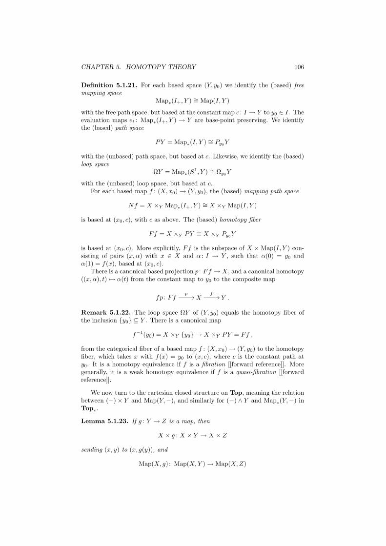
CHAPTER 5. HOMOTOPY THEORY 106
Definition 5.1.21. For each based space (Y, y0) we identify the (based) freemapping space
Map∗(I+, Y ) ∼= Map(I, Y )
with the free path space, but based at the constant map c : I → Y to y0 ∈ I. Theevaluation maps et : Map∗(I+, Y ) → Y are base-point preserving. We identifythe (based) path space
PY = Map∗(I, Y ) ∼= Py0Y
with the (unbased) path space, but based at c. Likewise, we identify the (based)loop space
ΩY = Map∗(S1, Y ) ∼= Ωy0
Y
with the (unbased) loop space, but based at c.For each based map f : (X,x0) → (Y, y0), the (based) mapping path space
Nf = X ×Y Map∗(I+, Y ) ∼= X ×Y Map(I, Y )
is based at (x0, c), with c as above. The (based) homotopy fiber
Ff = X ×Y PY ∼= X ×Y Py0Y
is based at (x0, c). More explicitly, Ff is the subspace of X × Map(I, Y ) con-sisting of pairs (x, α) with x ∈ X and α : I → Y , such that α(0) = y0 andα(1) = f(x), based at (x0, c).
There is a canonical based projection p : Ff → X, and a canonical homotopy((x, α), t) 7→ α(t) from the constant map to y0 to the composite map
fp : Ffp
// Xf
// Y .
Remark 5.1.22. The loop space ΩY of (Y, y0) equals the homotopy fiber ofthe inclusion y0 ⊆ Y . There is a canonical map
f−1(y0) = X ×Y y0 → X ×Y PY = Ff ,
from the categorical fiber of a based map f : (X,x0) → (Y, y0) to the homotopyfiber, which takes x with f(x) = y0 to (x, c), where c is the constant path aty0. It is a homotopy equivalence if f is a fibration [[forward reference]]. Moregenerally, it is a weak homotopy equivalence if f is a quasi-fibration [[forwardreference]].
We now turn to the cartesian closed structure on Top, meaning the relationbetween (−) × Y and Map(Y,−), and similarly for (−) ∧ Y and Map∗(Y,−) inTop∗.
Lemma 5.1.23. If g : Y → Z is a map, then
X × g : X × Y → X × Z
sending (x, y) to (x, g(y)), and
Map(X, g) : Map(X,Y ) → Map(X,Z)
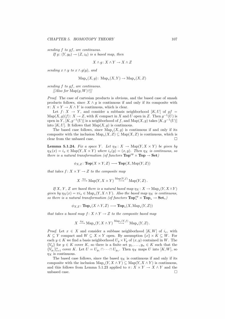
CHAPTER 5. HOMOTOPY THEORY 107
sending f to gf , are continuous.If g : (Y, y0) → (Z, z0) is a based map, then
X ∧ g : X ∧ Y → X ∧ Z
sending x ∧ y to x ∧ g(y), and
Map∗(X, g) : Map∗(X,Y ) → Map∗(X,Z)
sending f to gf , are continuous.[[Also for Map(g,W )?]]
Proof. The case of cartesian products is obvious, and the based case of smashproducts follows, since X ∧ g is continuous if and only if its composite withπ : X × Y → X ∧ Y is continuous, which is clear.
Let f : X → Y , and consider a subbasis neighborhood [K,U ] of gf =Map(X, g)(f) : X → Z, with K compact in X and U open in Z. Then g−1(U) isopen in Y , [K, g−1(U)] is a neighborhood of f , and Map(X, g) takes [K, g−1(U)]into [K,U ]. It follows that Map(X, g) is continuous.
The based case follows, since Map∗(X, g) is continuous if and only if itscomposite with the inclusion Map∗(X,Z) ⊆ Map(X,Z) is continuous, which isclear from the unbased case.
Lemma 5.1.24. Fix a space Y . Let ηX : X → Map(Y,X × Y ) be given byηX(x) = ix ∈ Map(Y,X × Y ) where ix(y) = (x, y). Then ηX is continuous, sothere is a natural transformation (of functors Topop × Top → Set)
φX,Z : Top(X × Y,Z) −→ Top(X,Map(Y,Z))
that takes f : X × Y → Z to the composite map
XηX−→ Map(Y,X × Y )
Map(Y,f)−→ Map(Y,Z) .
If X, Y , Z are based there is a natural based map ηX : X → Map∗(Y,X ∧Y )given by ηX(x) = πix ∈ Map∗(Y,X ∧Y ). Also the based map ηX is continuous,so there is a natural transformation (of functors Topop
∗ × Top∗ → Set∗)
φX,Z : Top∗(X ∧ Y,Z) −→ Top∗(X,Map∗(Y,Z))
that takes a based map f : X ∧ Y → Z to the composite based map
XηX−→ Map∗(Y,X ∧ Y )
Map∗(Y,f)−→ Map∗(Y,Z) .
Proof. Let x ∈ X and consider a subbase neighborhood [K,W ] of ix, withK ⊆ Y compact and W ⊆ X × Y open. By assumption x × K ⊆ W . Foreach y ∈ K we find a basis neighborhood Uy ×Vy of (x, y) contained in W . TheVy for y ∈ K cover K, so there is a finite set y1, . . . , yn ∈ K such that theVyi
ni=1 cover K. Let U = Uy1
∩ · · · ∩ Uyn. Then ηX maps U into [K,W ], so
ηX is continuous.The based case follows, since the based ηX is continuous if and only if its
composite with the inclusion Map∗(Y,X ∧ Y ) ⊆ Map(Y,X ∧ Y ) is continuous,and this follows from Lemma 5.1.23 applied to π : X × Y → X ∧ Y and theunbased case.
CHAPTER 5. HOMOTOPY THEORY 108
Definition 5.1.25. A space Y is locally compact if for any point y ∈ Y and eachopen neighborhood U ⊆ Y of y, there exists a smaller compact neighborhoodK ⊆ U of y.
Remark 5.1.26. For example, each compact Hausdorff space is locally com-pact, since y and the closed complement of U can be separated by open neigh-borhoods. The complement of the open neighborhood of U is then a closedneighborhood of y, which is compact.
Lemma 5.1.27. Fix a space Y . Let ǫZ : Map(Y,Z) × Y → Z be given byǫZ(f, y)) = f(y) ∈ Z where f : Y → Z and y ∈ Y . If Y is locally compact, thenǫZ is continuous, so there is a natural transformation
ψX,Z : Top(X,Map(Y,Z)) −→ Top(X × Y,Z)
that takes g : X → Map(Y,Z) to the composite map
X × Yg×Y−→ Map(Y,Z) × Y
ǫZ−→ Z .
If X, Y , Z are based there is a natural based map ǫZ : Map∗(Y,Z)∧Y → Zgiven by ǫZ(f ∧ y) = f(y) ∈ Z. If Y is locally compact then also the based mapǫZ is continuous, so there is a natural transformation
ψX,Z : Top∗(X,Map∗(Y,Z)) −→ Top∗(X ∧ Y,Z)
that takes a based map g : X → Map∗(Y,Z) to the composite based map
X ∧ Yg∧Y−→ Map∗(Y,Z) ∧ Y
ǫZ−→ Z .
Proof. Let (f, y) ∈ Map(Y,Z) × Y , and consider any open neighborhood Wof f(y) ∈ Z. Then f−1(W ) is an open neighborhood of y ∈ Y . By the keyassumption that Y is locally compact there exists a compact neighborhood K ⊆f−1(W ) of y in Y . Then [K,W ]×K is a neighborhood of (f, y) in Map(Y,Z)×Y ,and ǫZ takes it into W . Hence ǫZ is continuous.
Finally, the based ǫZ is continuous if and only if its composite with thecanonical map π : Map∗(Y,Z)×Y → Z is continuous, and this follows from theunbased case.
Proposition 5.1.28. Let Y be a locally compact space. There is a naturalbijection
φX,Z : Top(X × Y,Z) ∼= Top(X,Map(Y,Z))
that exhibits the functors X 7→ X × Y and Z 7→ Map(Y,Z) as the left and rightadjoint, respectively, in an adjoint pair.
Top(−)×Y
//Top
Map(Y,−)oo
The adjunction unit and counit are ηX : X → Map(Y,X×Y ) and ǫZ : Map(Y,Z)×Y → Z, respectively.
If X, Y , Z are based and Y is locally compact, there is also a natural bijection
φX,Z : Top∗(X ∧ Y,Z) ∼= Top∗(X,Map∗(Y,Z))
CHAPTER 5. HOMOTOPY THEORY 109
that exhibits the functors X 7→ X ∧Y and Z 7→ Map∗(Y,Z) as the left and rightadjoint, respectively, in an adjoint pair.
Top∗
(−)∧Y//Top∗
Map∗(Y,−)oo
The adjunction unit and counit are
ηX : X → Map∗(Y,X ∧ Y )
ǫZ : Map∗(Y,Z) ∧ Y → Z
respectively.
Proof. The composite
X × YηX×Y−→ Map(Y,X × Y ) × Y
ǫX×Y−→ X × Y
takes (x, y) first to (ix, y) and then to ix(y) = (x, y), hence equals the identity.It follows that the composite ψX,Z φX,Z is the identity, since it takes f : X ×Y → Z first to the composite Map(Y, f) ηX , and then to the composite ǫZ ((Map(Y, f) ηX)× Y ) = ǫZ (Map(Y, f)× Y ) (ηX × Y ), which by naturalityof ǫ equals f ǫX×Y (ηX × Y )) = f id = f .
Likewise, the composite
Map(Y,Z)ηMap(Y,Z)−→ Map(Y,Map(Y,Z) × Y )
Map(Y,ǫZ)−→ Map(Y,Z)
takes f first to if : y 7→ (f, y) and then to y 7→ f(y), hence equals the iden-tity. It follows that the composite φX,Z ψX,Z is the identity, since it takesg : X → Map(Y,Z) first to the composite ǫZ (g × Y ), and then to the com-posite Map(Y, ǫZ (g × Y )) ηX = Map(Y, ǫZ) Map(Y, g × Y ) ηX , which bynaturality of η with respect to g equals Map(Y, ǫZ) ηMap(Y,Z) g = id g = g.
The proof in the based case goes the same way.
Corollary 5.1.29. There are natural bijections
Top∗(X ∧ I+, Z) ∼= Top∗(X,Map∗(I+, Z))
Top∗(CX,Z) ∼= Top∗(X,PZ)
Top∗(ΣX,Z) ∼= Top∗(X,ΩZ)
for based spaces X, Z. Hence each based homotopy H : X ∧ I+ → Z from f to gcorresponds to a based map K : X → Map∗(I+, Z) with e0K = f and e1K = g,and conversely.
The adjunction unit in the third case is ηX : X → ΩΣX taking x to the basedloop s 7→ x∧ s for s ∈ S1, and the counit is ǫZ : ΣΩZ → Z taking s∧α to α(s),where α : S1 → Z is a based loop.
Proof. These are the special cases Y = I+, Y = I and Y = S1 of the previousproposition.
CHAPTER 5. HOMOTOPY THEORY 110
5.2 CW complexes
The definition of a topological space is general enough to allow many quiteill-behaved examples. However, the classifying spaces of categories, and mostof the other topological spaces that will be important for our study of higheralgebraic K-theory, are rather more well-behaved, in that they can be built upfrom nothing by successive attachments of cells. More precisely they are CWcomplexes, which we review in this section.
Definition 5.2.1. For n ≥ 0, let the n-disk
Dn = (x1, . . . , xn) ∈ Rn |n∑
i=1
x2i ≤ 1
be the unit ball in Euclidean n-space, and let the (n − 1)-sphere
Sn−1 = (x1, . . . , xn) ∈ Rn |n∑
i=1
x2i = 1
be its boundary, Sn−1 = ∂Dn. For n ≥ 1 we view Dn and Sn−1 as being basedat the point e1 = (1, 0, . . . , 0). Note that D0 is a point and S−1 = ∅.
[[Note that we here index the coordinates of Rn from 1 to n.]]
Definition 5.2.2. A CW complex is a space Y with a CW-structure, i.e., anincreasing skeleton filtration
∅ = Y (−1) ⊆ Y (0) ⊆ · · · ⊆ Y (n−1) ⊆ Y (n) ⊆ · · · ⊆ Y
where for each n ≥ 0 the n-skeleton Y (n) is obtained from the (n − 1)-skeletonby the adjunction of a set of n-cells along their boundaries, so that there is apushout square:
∐α Sn−1
²²
φn
//
p
Y (n−1)
²²∐α Dn Φn
// Y (n)
Here α runs through the set Y ♯n of n-cells in Y , the map φn is the coproduct of
maps φα : Sn−1 → Y (n−1), called the attaching maps, and the map Φn is the co-product of maps Φα : Dn → Y (n), called the characteristic maps. Furthermore,Y is the increasing union of its skeleta
Y =⋃
n≥0
Y (n) = colimn≥0
Y (n)
and is given the weak topology, meaning the finest topology such that eachinclusion Y (n) → Y is continuous. Equivalently, a subspace U ⊆ Y is open(resp. closed) if and only if each intersection Y (n) ∩ U is open (resp. closed)in Y (n), or equivalently, if each preimage Φ−1
α (U) is open (resp. closed) in Dn.
CHAPTER 5. HOMOTOPY THEORY 111
Definition 5.2.3. A CW complex Y is finite dimensional if there is an integerd such that Y has no n-cells for n > d. The minimal such d is then called thedimension of Y . A CW complex is of finite type if for each n ≥ 0 there areonly finitely many n-cells in Y . It is finite if it is finite dimensional and of finitetype, or equivalently, if the total number of cells in all dimensions is finite.
Lemma 5.2.4. A CW complex is finite if and only if it is compact as a topo-logical space.
Proof. [[If there are infinitely many cells, choose a non-repeating sequence (αi)∞i=1
of them. The center points xi in these cells then form a sequence in Y with noconvergent subsequence.]]
Definition 5.2.5. A map f : X → Y of CW complexes is cellular if f(X(n)) ⊆Y (n) for all n ≥ 0. CW complexes and cellular maps form a subcategory
CW ⊂ Top
of topological spaces. Note that this subcategory is not full.
[[Based CW complexes: two interpretations!]]
Definition 5.2.6. A closed subspace X of a CW complex Y is a subcomplexif for each n ≥ 0, the n-skeleton X(n) = X ∩ Y (n) is obtained by adjoining asubset X♯
n ⊆ Y ♯n of the n-cells in Y to the (n− 1)-skeleton X(n−1). We then say
that X ⊆ Y or (Y,X) a CW pair.
Lemma 5.2.7. Let X be a subcomplex of a CW complex Y . Then the subspacetopology on X equals the weak topology with respect to the subspaces X(n), sothat X is itself a CW complex. The inclusion X ⊆ Y is a cellular map.
Proof. A subset L ⊆ X is closed in the weak topology if and only if each X(n)∩Lis closed in X(n). Each X(n) is closed in Y (n), so this is equivalent to askingthat each Y (n) ∩L is closed in Y (n). This is the same as saying that L is closedin Y . Since X is closed in Y , this is equivalent to L ⊆ X being closed in thesubspace topology.
Lemma 5.2.8. Let Y , Z be CW complexes, X ⊆ Y a subcomplex, and f : X →Z a cellular map. Then Y ∪X Z is a CW complex, with n-skeleton
(Y ∪X Z)(n) = Y (n) ∪X(n) Z(n) ,
one n-cell for each n-cell in Y that is not contained in X, and one n-cell foreach n-cell in Z. The characteristic maps are the composites Dn → Y (n) →(Y ∪X Z)(n) and Dn → Z(n) → (Y ∪X Z)(n), respectively. The square
Xf
//
²²
p
Z
²²
Y // Y ∪X Z
is a pushout in CW.
CHAPTER 5. HOMOTOPY THEORY 112
Definition 5.2.9. Let X and Y be CW complexes, with characteristic mapsΦα and Ψβ . The product CW complex X × Y has n-skeleton
(X × Y )(n) =⋃
i+j=n
X(i) × Y (j)
for each n ≥ 0, and one (i+ j)-cell for each i-cell α in X and each j-cell β in Y ,with characteristic map
Θα,β : Di+j ∼= Di × Dj Φα×Ψβ−→ X(i) × Y (j) ⊆ X(i+j) .
Its restriction to the boundary
Si+j−1 = ∂Di+j ∼= ∂(Di × Dj) = Si−1 × Dj ∪ Di × Sj−1
factors through the attaching map
θα,β : Si+j−1 ∼= Si−1 ∪ Dj ∪ Di × Sj−1
−→ X(i−1) × Y (j) ∪ X(i) × Y (j−1) ⊆ X(i+j−1) .
The product X×Y has the weak topology with respect to the skeleton filtration,or equivalently, with respect to all of the characteristic maps Θα,β .
The projection maps pr1 : X × Y → X and pr2 : X × Y → Y are cellular,and X × Y is the product in CW of X and Y .
Remark 5.2.10. Note that the weak topology on the product CW complexX ×Y is not always the same as the product topology on the cartesian productX × Y , formed in Top. There is a map from the CW product with the weaktopology, to the cartesian product with the product topology, but it is notin general a homeomorphism. [[Example?]] This suggests that the cartesianproduct topology, which is the coarsest topology making the projections to Xand Y continuous, is too coarse, and that we should instead give X × Y a finertopology that agrees with the weak topology on a product of CW complexes inthe case when X and Y are CW complexes. This is what is achieved with thecompactly generated topology.
The following three lemmas are trivial to prove.
Lemma 5.2.11. Let X ⊆ Y be a CW pair and Z a CW complex. Then
X × Z ⊆ Y × Z
is a CW pair.
Lemma 5.2.12. Let X and Y be subcomplexes of a CW complex Z. ThenX ∩ Y and X ∪ Y are also subcomplexes of Z.
Lemma 5.2.13. Let X ⊆ Y and Z ⊆ W be CW pairs. Then
X × W ∪X×Z Y × Z ⊆ Y × W
is a CW pair.
[[Cite Milnor on the homotopy type of Map(X,Y ) for X, Y CW complexes,with X finite?]]
CHAPTER 5. HOMOTOPY THEORY 113
5.3 Compactly generated spaces
[[Steenrod [62], McCord [45], May [43, Ch. 5].]][[Weak Hausdorff spaces, (Kelley) k-spaces, compactly generated spaces U
and T , closure under closed cobase change, closed sequential colimits, adjunc-tion
Map(X × Y,Z) ∼= Map(X,Map(Y,Z))
is a homeomorphism. Space = compactly generated space, based space = cofi-brantly based compactly generated space.]]
5.4 Cofibrations
For more about cofibrations we refer to May [43, Ch. 6] and Hatcher [26, Ch. 0].
Definition 5.4.1. A map i : X → Y is said to have the homotopy extensionproperty (HEP) with respect to a space T if for any commutative diagram ofsolid arrows
Xi0 //
i
²²
X × I
i×id
²²H
³³
Yi0 //
f //
Y × I
FF
F
""FF
T
there exists a dashed arrow making the whole diagram commute. The map i iscalled a cofibration if it has the homotopy extension property with respect toany space T . We often use a feathered arrow i : X Y to indicate that i is acofibration.
Remark 5.4.2. In words and symbols, the homotopy extension property withrespect to T asks that given a map f : Y → T and a homotopy H : X × I → Tstarting with the composite map fi : X → T , there exists a homotopy F : Y ×I → T starting with f , such that F (i × id) = H.
Lemma 5.4.3. A map i : X → Y is a cofibration if and only if the induced mapj = i0 ∪ (i × id) : Y ∪X X × I → Y × I admits a left inverse
r : Y × I → Y ∪X X × I .
Proof. This is clear from the universal case T = Y ∪X X × I, with f : Y → Tand H : X × I → T the obvious inclusions.
Here is a basic example.
Lemma 5.4.4. The inclusion Sn−1 ⊂ Dn is a cofibration for each n ≥ 0.
Proof. View Dn×I as a subspace of Rn×R. There is a (deformation) retractionr : Dn × I → Dn ×0 ∪Sn−1 × I given by linear projection away from (0, 2) ∈Rn × R, so Sn−1
Dn.
Lemma 5.4.5. Each cofibration (in U ) is a closed embedding.
CHAPTER 5. HOMOTOPY THEORY 114
Proof. Let r be left inverse to j, as above. The composite
Xi
−→ Yi1−→ Y × I
r−→ Y ∪X X × I
equals the embedding i1 : X → Y ∪X X×I. Hence i must also be an embedding.(The open subsets of X are of the form i−1
1 (U) with U open in Y ∪X X×I, henceare also of the form i−1(V ) with V = (ri1)
−1(U) open in Y .) The subspace
B = x ∈ Y | jr(x, 1) = (x, 1)
is equal to the image i(X) of i, and is closed in Y since Y is weak Hausdorff.
Lemma 5.4.6. A map i : X → Y is a cofibration if and only if it has the leftlifting property with respect to the free path fibration e0 : Map(I, T ) → T forany space T , i.e., given any commutative diagram of solid arrows
XH //
i
²²
Map(I, T )
e0
²²
Yf
//
Fuuu
::uu
T
there exists a dashed arrow making the whole diagram commute.
Proof. This is immediate from the isomorphism
Top(Y × I, T ) ∼= Top(Y,Map(I, T ))
and its variants.
Lemma 5.4.7. Each homeomorphism is a cofibration, and the composite oftwo cofibrations is a cofibration, so the cofibrations form a subcategory of thecategory of topological spaces.
Proof. For the first claim, let F = Hi−1, with notation as above.If i : X Y and j : Y Z are cofibrations, then given a commutative
diagram of solid arrows
XH //
²²
i
²²
Map(I, T )
e0
²²
Y²²
j
²²
Fuu
::uu
Zf
//
G¨¨
¨¨
CC¨¨
¨¨
T
we use the left lifting property for i to find the dashed arrow F , and then usethe left lifting property for j to find the dashed arrow G, making the wholediagram commute. Hence ji : X Z is a cofibration.
Lemma 5.4.8. (a) The coproduct X =∐
α Xα ∐
α Yα = Y of any set ofcofibrations iα : Xα Yα is a cofibration.
(b) The pushout (= cobase change) Z Y ∪X Z of a cofibration i : X Yalong any map j : X → Z is a cofibration.
CHAPTER 5. HOMOTOPY THEORY 115
(c) The composite Y−1 Y of a sequence of cofibrations in : Yn−1 Yn forn ≥ 0, with Y = colimn Yn, is a cofibration.
Proof. (a): Construct a lift Fα : Yα → Map(I, T ) for each α, and assemble theseto a lift F : Y → Map(I, T ).
(b): A left lifting problem for Z → Y ∪X Z amounts to a diagram of solidarrows:
Xf
//
²²
i
²²
p
ZH //
²²
Map(I, T )
e0
²²
Y //
Fiiiiii
44iiii
Y ∪X Zg
//
Gqqq
88qq
T
The assumption that i is a cofibration gives the dashed arrow F . The fact thatthe left hand square is a pushout gives the dashed arrow G, making the wholediagram commute.
(c): A left lifting problem for Y−1 → Y is given by the solid arrows in thefollowing diagram, which is flipped over for typographical reasons.
Y−1// //
H
²²
. . . // // Yn−1//
in //
Fn−1t
tt
tt
zztt
tt
t
Yn// //
Fnn n n n n n n
vvn n n n n n
. . . // // Y
f
²²
Fi i i i i i i i i i i i
tti i i i i i i i i i
Map(I, T )e0 // T
Assume inductively for n ≥ 0 that we have filled in the arrow Fn−1 : Yn−1 →Map(I, T ), starting the induction with F−1 = H. Using the left lifting propertyfor in, we can fill in the arrow Fn : Yn → Map(I, T ), still keeping the diagramcommutative. Now let F : Y → Map(I, T ) be the colimit of the maps Fn. It iscontinuous, because Y = colimn Yn is given the (weak) colimit topology.
Proposition 5.4.9. The inclusion X ⊆ Y of a subcomplex in a CW complexis a cofibration.
Proof. Let Yn = X ∪ Y (n) ⊆ Y , for each n ≥ −1. Hence there is a pushoutsquare ∐
α Sn−1 //
²²
p
Yn−1
in
²²∐α Dn // Yn
for each n ≥ 0, where α ranges over the n-cells in Y that are not in X. ByLemmas 5.4.4 and 5.4.8, all the inclusions Sn−1 → Dn,
∐α Sn−1 →
∐α Dn,
in : Yn−1 → Yn and X = Y−1 → Y are cofibrations.
Lemma 5.4.10. Let f : X → Y be any map. The inclusion
X × 0 ⊔ Y Mf
is a cofibration. Hence so are the inclusions i0 : X → Mf , Y → Mf andi : Y → Cf .
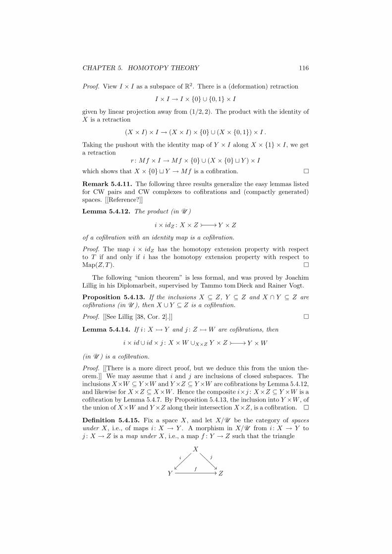
CHAPTER 5. HOMOTOPY THEORY 116
Proof. View I × I as a subspace of R2. There is a (deformation) retraction
I × I → I × 0 ∪ 0, 1 × I
given by linear projection away from (1/2, 2). The product with the identity ofX is a retraction
(X × I) × I → (X × I) × 0 ∪ (X × 0, 1) × I .
Taking the pushout with the identity map of Y × I along X × 1 × I, we geta retraction
r : Mf × I → Mf × 0 ∪ (X × 0 ⊔ Y ) × I
which shows that X × 0 ⊔ Y → Mf is a cofibration.
Remark 5.4.11. The following three results generalize the easy lemmas listedfor CW pairs and CW complexes to cofibrations and (compactly generated)spaces. [[Reference?]]
Lemma 5.4.12. The product (in U )
i × idZ : X × Z // // Y × Z
of a cofibration with an identity map is a cofibration.
Proof. The map i × idZ has the homotopy extension property with respectto T if and only if i has the homotopy extension property with respect toMap(Z, T ).
The following “union theorem” is less formal, and was proved by JoachimLillig in his Diplomarbeit, supervised by Tammo tom Dieck and Rainer Vogt.
Proposition 5.4.13. If the inclusions X ⊆ Z, Y ⊆ Z and X ∩ Y ⊆ Z arecofibrations (in U ), then X ∪ Y ⊆ Z is a cofibration.
Proof. [[See Lillig [38, Cor. 2].]]
Lemma 5.4.14. If i : X Y and j : Z W are cofibrations, then
i × id ∪ id × j : X × W ∪X×Z Y × Z // // Y × W
(in U ) is a cofibration.
Proof. [[There is a more direct proof, but we deduce this from the union the-orem.]] We may assume that i and j are inclusions of closed subspaces. Theinclusions X×W ⊆ Y ×W and Y ×Z ⊆ Y ×W are cofibrations by Lemma 5.4.12,and likewise for X×Z ⊆ X×W . Hence the composite i×j : X×Z ⊆ Y ×W is acofibration by Lemma 5.4.7. By Proposition 5.4.13, the inclusion into Y ×W , ofthe union of X×W and Y ×Z along their intersection X×Z, is a cofibration.
Definition 5.4.15. Fix a space X, and let X/U be the category of spacesunder X, i.e., of maps i : X → Y . A morphism in X/U from i : X → Y toj : X → Z is a map under X, i.e., a map f : Y → Z such that the triangle
Xi
~~~~~~
~~~
j
ÃÃ@@
@@@@
@
Yf
// Z
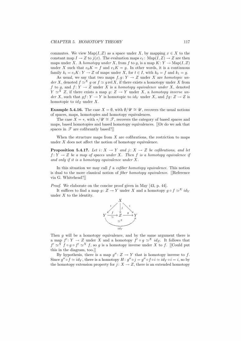
CHAPTER 5. HOMOTOPY THEORY 117
commutes. We view Map(I, Z) as a space under X, by mapping x ∈ X to theconstant map I → Z to j(x). The evaluation maps et : Map(I, Z) → Z are thenmaps under X. A homotopy under X, from f to g, is a map K : Y → Map(I, Z)under X such that e0K = f and e1K = g. In other words, it is a continuousfamily kt = etK : Y → Z of maps under X, for t ∈ I, with k0 = f and k1 = g.
As usual, we say that two maps f, g : Y → Z under X are homotopic un-der X, denoted f ≃X g or f ≃ g relX, if there exists a homotopy under X fromf to g, and f : Y → Z under X is a homotopy equivalence under X, denotedY ≃X Z, if there exists a map g : Z → Y under X, a homotopy inverse un-der X, such that gf : Y → Y is homotopic to idY under X, and fg : Z → Z ishomotopic to idZ under X.
Example 5.4.16. The case X = ∅, with ∅/U ∼= U , recovers the usual notionsof spaces, maps, homotopies and homotopy equivalences.
The case X = ∗, with ∗/U ∼= T , recovers the category of based spaces andmaps, based homotopies and based homotopy equivalences. [[Or do we ask thatspaces in T are cofibrantly based?]]
When the structure maps from X are cofibrations, the restriction to mapsunder X does not affect the notion of homotopy equivalence.
Proposition 5.4.17. Let i : X → Y and j : X → Z be cofibrations, and letf : Y → Z be a map of spaces under X. Then f is a homotopy equivalence ifand only if it is a homotopy equivalence under X.
In this situation we may call f a cofiber homotopy equivalence. This notionis dual to the more classical notion of fiber homotopy equivalence. [[Referencevia G. Whitehead?]]
Proof. We elaborate on the concise proof given in May [43, p. 44].It suffices to find a map g : Z → Y under X and a homotopy g f ≃X idY
under X to the identity.
Xi
~~~~~~
~~~
j
²²
i
ÃÃ@@
@@@@
@
Yf
≃//
idY
JJZg
//
≃X
Y
Then g will be a homotopy equivalence, and by the same argument there isa map f ′ : Y → Z under X and a homotopy f ′ g ≃X idZ . It follows thatf ′ ≃X f g f ′ ≃X f , so g is a homotopy inverse under X to f . [[Could putthis in the diagram, too.]]
By hypothesis, there is a map g′′ : Z → Y that is homotopy inverse to f .Since g′′ f ≃ idY , there is a homotopy H : g′′ j = g′′ f i ≃ idY i = i, so bythe homotopy extension property for j : X → Z, there is an extended homotopy
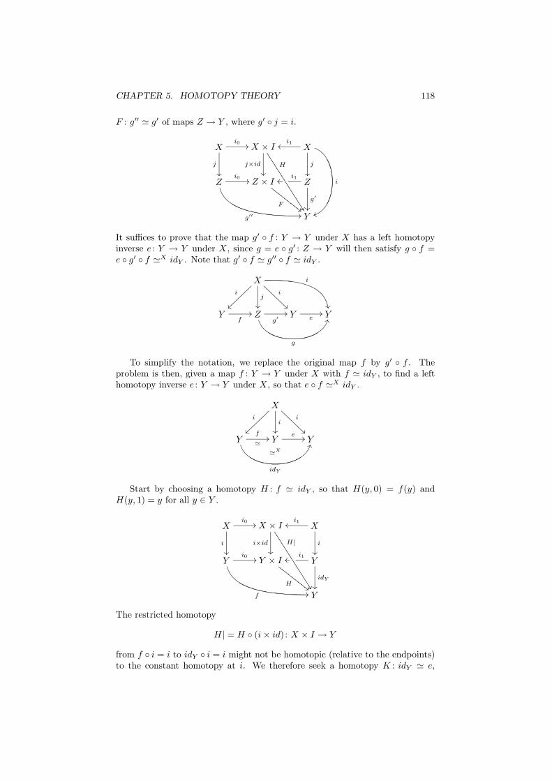
CHAPTER 5. HOMOTOPY THEORY 118
F : g′′ ≃ g′ of maps Z → Y , where g′ j = i.
Xi0 //
j
²²
X × I
j×id
²²
H
¼¼33
3333
3333
3333
3 Xi1oo
i
tt
j
²²
Zi0 //
g′′ //
Z × I
F##FF
FFFF
FFF Z
i1oo
g′
²²
Y
It suffices to prove that the map g′ f : Y → Y under X has a left homotopyinverse e : Y → Y under X, since g = e g′ : Z → Y will then satisfy g f =e g′ f ≃X idY . Note that g′ f ≃ g′′ f ≃ idY .
Xi
~~~~~~
~~~
j
²²
i
ÃÃ@@
@@@@
@ i
´´
Yf
// Zg′
//
g
JJY e// Y
To simplify the notation, we replace the original map f by g′ f . Theproblem is then, given a map f : Y → Y under X with f ≃ idY , to find a lefthomotopy inverse e : Y → Y under X, so that e f ≃X idY .
Xi
~~~~~~
~~~
i
²²
i
ÃÃ@@
@@@@
@
Yf
≃//
idY
JJYe //
≃X
Y
Start by choosing a homotopy H : f ≃ idY , so that H(y, 0) = f(y) andH(y, 1) = y for all y ∈ Y .
Xi0 //
i
²²
X × I
i×id
²²
H|
¼¼33
3333
3333
3333
3 Xi1oo
i
²²
Yi0 //
f //
Y × I
H##FF
FFFF
FFF Y
i1oo
idY
²²
Y
The restricted homotopy
H| = H (i × id) : X × I → Y
from f i = i to idY i = i might not be homotopic (relative to the endpoints)to the constant homotopy at i. We therefore seek a homotopy K : idY ≃ e,
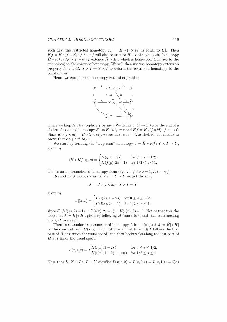
CHAPTER 5. HOMOTOPY THEORY 119
such that the restricted homotopy K| = K (i × id) is equal to H|. ThenKf = K (f × id) : f ≃ ef will also restrict to H|, so the composite homotopyH ∗ Kf : idY ≃ f ≃ e f extends H| ∗ H|, which is homotopic (relative to theendpoints) to the constant homotopy. We will then use the homotopy extensionproperty for i × id : X × I → Y × I to deform the restricted homotopy to theconstant one.
Hence we consider the homotopy extension problem
Xi0 //
i
²²
X × I
i×id
²²
H|
¼¼33
3333
3333
3333
3 Xi1oo
i
²²
Yi0 //
idY//
Y × I
K##F
FF
FF Y
i1oo
e
²²ÂÂÂ
Y
where we keep H|, but replace f by idY . We define e : Y → Y to be the end of achoice of extended homotopy K, so K : idY ≃ e and Kf = K(f×id) : f ≃ ef .Since K (i× id) = H (i× id), we see that e i = i, as desired. It remains toprove that e f ≃X idY .
We start by forming the “loop sum” homotopy J = H ∗ Kf : Y × I → Y ,given by
(H ∗ Kf)(y, s) =
H(y, 1 − 2s) for 0 ≤ s ≤ 1/2,
K(f(y), 2s − 1) for 1/2 ≤ s ≤ 1.
This is an s-parametrized homotopy from idY , via f for s = 1/2, to e f .Restricting J along i × id : X × I → Y × I, we get the map
J | = J (i × id) : X × I → Y
given by
J |(x, s) =
H(i(x), 1 − 2s) for 0 ≤ s ≤ 1/2,
H(i(x), 2s − 1) for 1/2 ≤ s ≤ 1,
since K(f(i(x), 2s− 1) = K(i(x), 2s− 1) = H(i(x), 2s− 1). Notice that this theloop sum J | = H| ∗H|, given by following H from i to i, and then backtrackingalong H to i again.
There is a standard t-parametrized homotopy L from the path J | = H| ∗H|to the constant path C(x, s) = i(x) at i, which at time t ∈ I follows the firstpart of H at t times the usual speed, and then backtracks along the last part ofH at t times the usual speed.
L(x, s, t) =
H(i(x), 1 − 2st) for 0 ≤ s ≤ 1/2,
H(i(x), 1 − 2(1 − s)t) for 1/2 ≤ s ≤ 1.
Note that L : X × I × I → Y satisfies L(x, s, 0) = L(x, 0, t) = L(x, 1, t) = i(x)
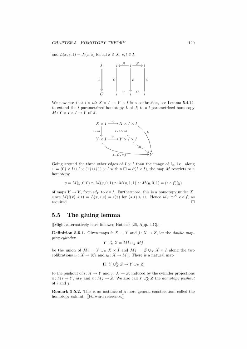
CHAPTER 5. HOMOTOPY THEORY 120
and L(x, s, 1) = J |(x, s) for all x ∈ X, s, t ∈ I.
J |
L
®¶
i
C
iHoo H //
H
²²
i
C
C iC
iC
i
We now use that i × id : X × I → Y × I is a cofibration, see Lemma 5.4.12,to extend the t-parametrized homotopy L of J | to a t-parametrized homotopyM : Y × I × I → Y of J .
X × Ii0 //
i×id
²²
X × I × I
i×id×id
²²L
³³
Y × Ii0 //
J=H∗Kf//
Y × I × I
MJ
J
$$JJJ
Y
Going around the three other edges of I × I than the image of i0, i.e., along⊔ = 0 × I ∪ I × 1 ∪ 1 × I within ¤ = ∂(I × I), the map M restricts to ahomotopy
y = M(y, 0, 0) ≃ M(y, 0, 1) ≃ M(y, 1, 1) ≃ M(y, 0, 1) = (e f)(y)
of maps Y → Y , from idY to e f . Furthermore, this is a homotopy under X,since M(i(x), s, t) = L(x, s, t) = i(x) for (s, t) ∈ ⊔. Hence idY ≃X e f , asrequired.
5.5 The gluing lemma
[[Might alternatively have followed Hatcher [26, App. 4.G].]]
Definition 5.5.1. Given maps i : X → Y and j : X → Z, let the double map-ping cylinder
Y ∪hX Z = Mi ∪X Mj
be the union of Mi = Y ∪X X × I and Mj = Z ∪X X × I along the twocofibrations i0 : X → Mi and i0 : X → Mj. There is a natural map
Π: Y ∪hX Z → Y ∪X Z
to the pushout of i : X → Y and j : X → Z, induced by the cylinder projectionsπ : Mi → Y , idX and π : Mj → Z. We also call Y ∪h
X Z the homotopy pushoutof i and j.
Remark 5.5.2. This is an instance of a more general construction, called thehomotopy colimit. [[Forward reference.]]
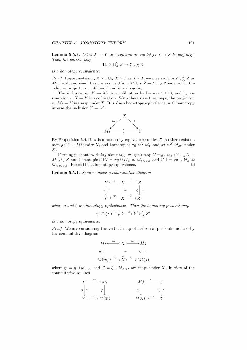
CHAPTER 5. HOMOTOPY THEORY 121
Lemma 5.5.3. Let i : X → Y be a cofibration and let j : X → Z be any map.Then the natural map
Π: Y ∪hX Z → Y ∪X Z
is a homotopy equivalence.
Proof. Reparametrizing X × I ∪X X × I as X × I, we may rewrite Y ∪hX Z as
Mi∪X Z, and view Π as the map π ∪ idZ : Mi∪X Z → Y ∪X Z induced by thecylinder projection π : Mi → Y and idZ along idX .
The inclusion i0 : X → Mi is a cofibration by Lemma 5.4.10, and by as-sumption i : X → Y is a cofibration. With these structure maps, the projectionπ : Mi → Y is a map under X. It is also a homotopy equivalence, with homotopyinverse the inclusion Y → Mi.
X
i0
ÃÃ
i
ÃÃ@@
@@@@
@
Miπ
≃// Y
By Proposition 5.4.17, π is a homotopy equivalence under X, so there exists amap g : Y → Mi under X, and homotopies πg ≃X idY and gπ ≃X idMi underX.
Forming pushouts with idZ along idX , we get a map G = g∪idZ : Y ∪X Z →Mi ∪X Z and homotopies ΠG = πg ∪ idZ ≃ idY ∪XZ and GΠ = gπ ∪ idZ ≃idMi∪XZ . Hence Π is a homotopy equivalence.
Lemma 5.5.4. Suppose given a commutative diagram
Y
η ≃
²²
Xioo
j//
=
²²
Z
ζ ≃
²²
Y ′ Xηi
ooζj
// Z ′
where η and ζ are homotopy equivalences. Then the homotopy pushout map
η ∪h ζ : Y ∪hX Z
≃−→ Y ′ ∪h
X Z ′
is a homotopy equivalence.
Proof. We are considering the vertical map of horizontal pushouts induced bythe commutative diagram
Mi
η′ ≃
²²
Xooi0oo //
i0 //
=
²²
Mj
ζ′ ≃
²²
M(ηi) Xooi0oo //
i0 // M(ζj)
where η′ = η ∪ idX×I and ζ ′ = ζ ∪ idX×I are maps under X. In view of thecommutative squares
Y≃ //
η ≃
²²
Mi
η′
²²
Mj
ζ′
²²
Z≃oo
ζ ≃
²²
Y ′ ≃ // M(ηi) M(ζj) Z ′≃oo
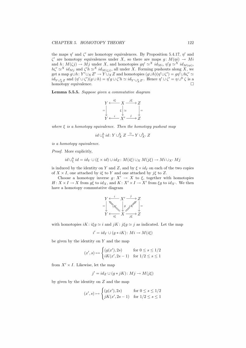
CHAPTER 5. HOMOTOPY THEORY 122
the maps η′ and ζ ′ are homotopy equivalences. By Proposition 5.4.17, η′ andζ ′ are homotopy equivalences under X, so there are maps g : M(ηi) → Miand h : M(ζj) → Mj under X, and homotopies gη′ ≃X idMi, η′g ≃X idM(ηi),hζ ′ ≃X idMj and ζ ′h ≃X idM(ζj), all under X. Forming pushouts along X, weget a map g∪h : Y ′∪X Z ′ → Y ∪X Z and homotopies (g∪h)(η′∪ζ ′) = gη′∪hζ ′ ≃idY ∪h
XZ and (η′ ∪ ζ ′)(g ∪ h) = η′g ∪ ζ ′h ≃ idY ′∪h
XZ′ . Hence η′ ∪ ζ ′ = η ∪h ζ is a
homotopy equivalence.
Lemma 5.5.5. Suppose given a commutative diagram
Y
=
²²
Xiξ
oojξ
//
ξ ≃
²²
Z
=
²²
Y X ′iooj
// Z
where ξ is a homotopy equivalence. Then the homotopy pushout map
id ∪hξ id : Y ∪h
X Z≃−→ Y ∪h
X′ Z
is a homotopy equivalence.
Proof. More explicitly,
id ∪hξ id = idY ∪ (ξ × id) ∪ idZ : M(iξ) ∪X M(jξ) → Mi ∪X′ Mj
is induced by the identity on Y and Z, and by ξ × idI on each of the two copiesof X × I, one attached by iξ to Y and one attached by jξ to Z.
Choose a homotopy inverse g : X ′ → X to ξ, together with homotopiesH : X × I → X from gξ to idX , and K : X ′ × I → X ′ from ξg to idX′ . We thenhave a homotopy commutative diagram
Y
=
²²
X ′iooj
//
g
²²
Z
=
²²
Y Xiξ
oojξ
//
iKAAAAAA
\dAAAAAA
jK
:B
Z
with homotopies iK : iξg ≃ i and jK : jξg ≃ j as indicated. Let the map
i′ = idY ∪ (g ∗ iK) : Mi → M(iξ)
be given by the identity on Y and the map
(x′, s) 7→
(g(x′), 2s) for 0 ≤ s ≤ 1/2
iK(x′, 2s − 1) for 1/2 ≤ s ≤ 1
from X ′ × I. Likewise, let the map
j′ = idZ ∪ (g ∗ jK) : Mj → M(jξ)
by given by the identity on Z and the map
(x′, s) 7→
(g(x′), 2s) for 0 ≤ s ≤ 1/2
jK(x′, 2s − 1) for 1/2 ≤ s ≤ 1
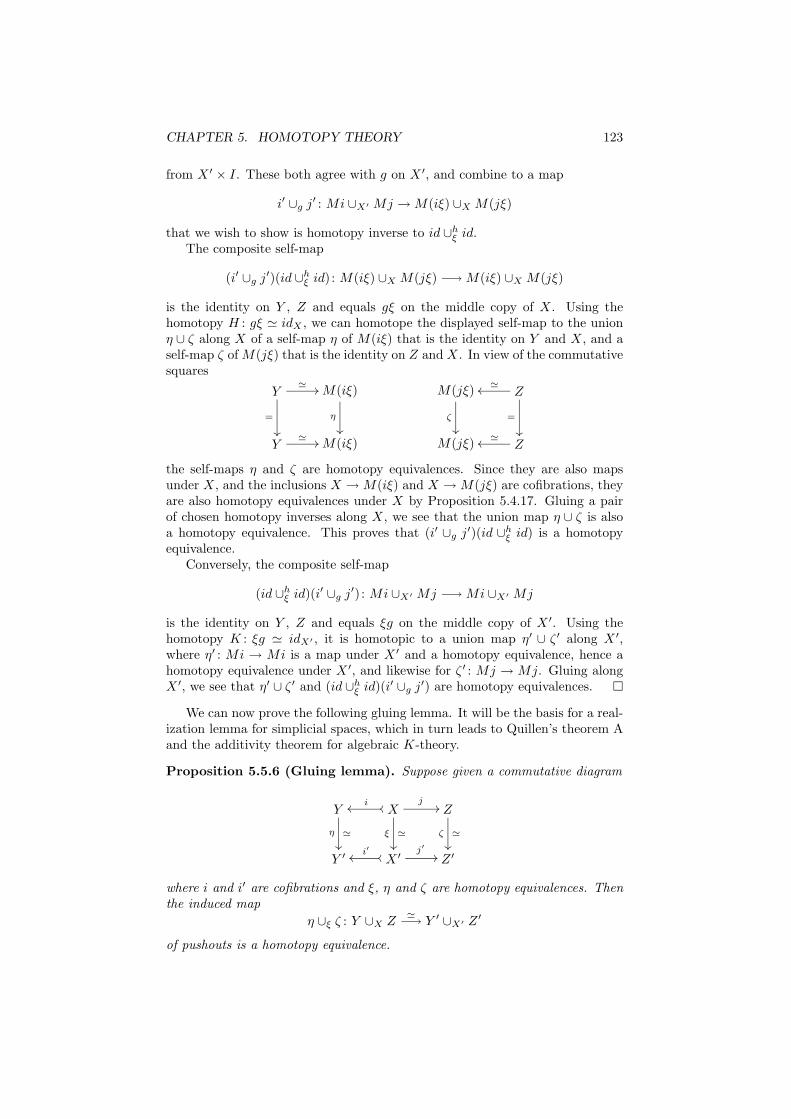
CHAPTER 5. HOMOTOPY THEORY 123
from X ′ × I. These both agree with g on X ′, and combine to a map
i′ ∪g j′ : Mi ∪X′ Mj → M(iξ) ∪X M(jξ)
that we wish to show is homotopy inverse to id ∪hξ id.
The composite self-map
(i′ ∪g j′)(id ∪hξ id) : M(iξ) ∪X M(jξ) −→ M(iξ) ∪X M(jξ)
is the identity on Y , Z and equals gξ on the middle copy of X. Using thehomotopy H : gξ ≃ idX , we can homotope the displayed self-map to the unionη ∪ ζ along X of a self-map η of M(iξ) that is the identity on Y and X, and aself-map ζ of M(jξ) that is the identity on Z and X. In view of the commutativesquares
Y≃ //
=
²²
M(iξ)
η
²²
M(jξ)
ζ
²²
Z≃oo
=
²²
Y≃ // M(iξ) M(jξ) Z
≃oo
the self-maps η and ζ are homotopy equivalences. Since they are also mapsunder X, and the inclusions X → M(iξ) and X → M(jξ) are cofibrations, theyare also homotopy equivalences under X by Proposition 5.4.17. Gluing a pairof chosen homotopy inverses along X, we see that the union map η ∪ ζ is alsoa homotopy equivalence. This proves that (i′ ∪g j′)(id ∪h
ξ id) is a homotopyequivalence.
Conversely, the composite self-map
(id ∪hξ id)(i′ ∪g j′) : Mi ∪X′ Mj −→ Mi ∪X′ Mj
is the identity on Y , Z and equals ξg on the middle copy of X ′. Using thehomotopy K : ξg ≃ idX′ , it is homotopic to a union map η′ ∪ ζ ′ along X ′,where η′ : Mi → Mi is a map under X ′ and a homotopy equivalence, hence ahomotopy equivalence under X ′, and likewise for ζ ′ : Mj → Mj. Gluing alongX ′, we see that η′ ∪ ζ ′ and (id ∪h
ξ id)(i′ ∪g j′) are homotopy equivalences.
We can now prove the following gluing lemma. It will be the basis for a real-ization lemma for simplicial spaces, which in turn leads to Quillen’s theorem Aand the additivity theorem for algebraic K-theory.
Proposition 5.5.6 (Gluing lemma). Suppose given a commutative diagram
Y
η ≃
²²
Xooiooj
//
ξ ≃
²²
Z
ζ ≃
²²
Y ′ X ′ooi′ooj′
// Z ′
where i and i′ are cofibrations and ξ, η and ζ are homotopy equivalences. Thenthe induced map
η ∪ξ ζ : Y ∪X Z≃−→ Y ′ ∪X′ Z ′
of pushouts is a homotopy equivalence.
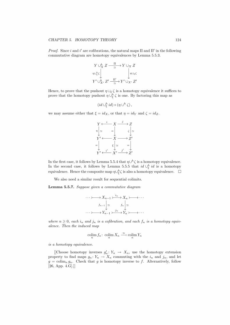
CHAPTER 5. HOMOTOPY THEORY 124
Proof. Since i and i′ are cofibrations, the natural maps Π and Π′ in the followingcommutative diagram are homotopy equivalences by Lemma 5.5.3.
Y ∪hX Z
Π
≃//
η∪hξ ζ
²²
Y ∪X Z
η∪ξζ
²²
Y ′ ∪hX′ Z ′ Π′
≃// Y ′ ∪X′ Z ′
Hence, to prove that the pushout η ∪ξ ζ is a homotopy equivalence it suffices toprove that the homotopy pushout η ∪h
ξ ζ is one. By factoring this map as
(id ∪hξ id) (η ∪h ζ) ,
we may assume either that ξ = idX , or that η = idY and ζ = idZ .
Y
η ≃
²²
Xioo
j//
=
²²
Z
ζ ≃
²²
Y ′
=
²²
Xoo //
ξ ≃
²²
Z ′
=
²²
Y ′ X ′i′ooj′
// Z ′
In the first case, it follows by Lemma 5.5.4 that η∪hζ is a homotopy equivalence.In the second case, it follows by Lemma 5.5.5 that id ∪h
ξ id is a homotopy
equivalence. Hence the composite map η∪hξ ζ is also a homotopy equivalence.
We also need a similar result for sequential colimits.
Lemma 5.5.7. Suppose given a commutative diagram
. . . // // Xn−1//
in //
fn−1 ≃
²²
Xn// //
fn ≃
²²
. . .
. . . // // Yn−1//
jn // Yn// // . . .
where n ≥ 0, each in and jn is a cofibration, and each fn is a homotopy equiv-alence. Then the induced map
colimn
fn : colimn
Xn≃−→ colim
nYn
is a homotopy equivalence.
[[Choose homotopy inverses g′n : Yn → Xn, use the homotopy extensionproperty to find maps gn : Yn → Xn commuting with the in and jn, and letg = colimn gn. Check that g is homotopy inverse to f . Alternatively, follow[26, App. 4.G].]]
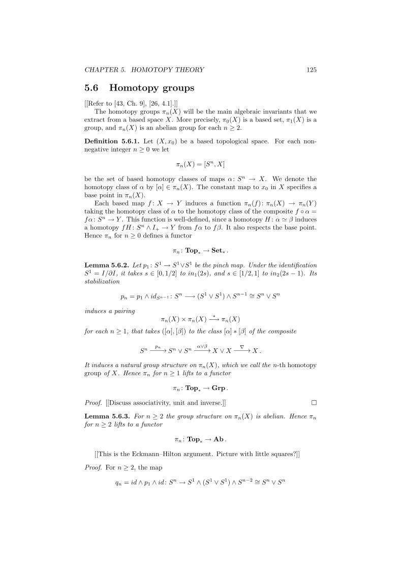
CHAPTER 5. HOMOTOPY THEORY 125
5.6 Homotopy groups
[[Refer to [43, Ch. 9], [26, 4.1].]]The homotopy groups πn(X) will be the main algebraic invariants that we
extract from a based space X. More precisely, π0(X) is a based set, π1(X) is agroup, and πn(X) is an abelian group for each n ≥ 2.
Definition 5.6.1. Let (X,x0) be a based topological space. For each non-negative integer n ≥ 0 we let
πn(X) = [Sn,X]
be the set of based homotopy classes of maps α : Sn → X. We denote thehomotopy class of α by [α] ∈ πn(X). The constant map to x0 in X specifies abase point in πn(X).
Each based map f : X → Y induces a function πn(f) : πn(X) → πn(Y )taking the homotopy class of α to the homotopy class of the composite f α =fα : Sn → Y . This function is well-defined, since a homotopy H : α ≃ β inducesa homotopy fH : Sn ∧ I+ → Y from fα to fβ. It also respects the base point.Hence πn for n ≥ 0 defines a functor
πn : Top∗ → Set∗ .
Lemma 5.6.2. Let p1 : S1 → S1∨S1 be the pinch map. Under the identificationS1 = I/∂I, it takes s ∈ [0, 1/2] to in1(2s), and s ∈ [1/2, 1] to in2(2s − 1). Itsstabilization
pn = p1 ∧ idSn−1 : Sn −→ (S1 ∨ S1) ∧ Sn−1 ∼= Sn ∨ Sn
induces a pairingπn(X) × πn(X)
∗−→ πn(X)
for each n ≥ 1, that takes ([α], [β]) to the class [α] ∗ [β] of the composite
Snpn // Sn ∨ Sn
α∨β// X ∨ X
∇ // X .
It induces a natural group structure on πn(X), which we call the n-th homotopygroup of X. Hence πn for n ≥ 1 lifts to a functor
πn : Top∗ → Grp .
Proof. [[Discuss associativity, unit and inverse.]]
Lemma 5.6.3. For n ≥ 2 the group structure on πn(X) is abelian. Hence πn
for n ≥ 2 lifts to a functor
πn : Top∗ → Ab .
[[This is the Eckmann–Hilton argument. Picture with little squares?]]
Proof. For n ≥ 2, the map
qn = id ∧ p1 ∧ id : Sn → S1 ∧ (S1 ∨ S1) ∧ Sn−2 ∼= Sn ∨ Sn
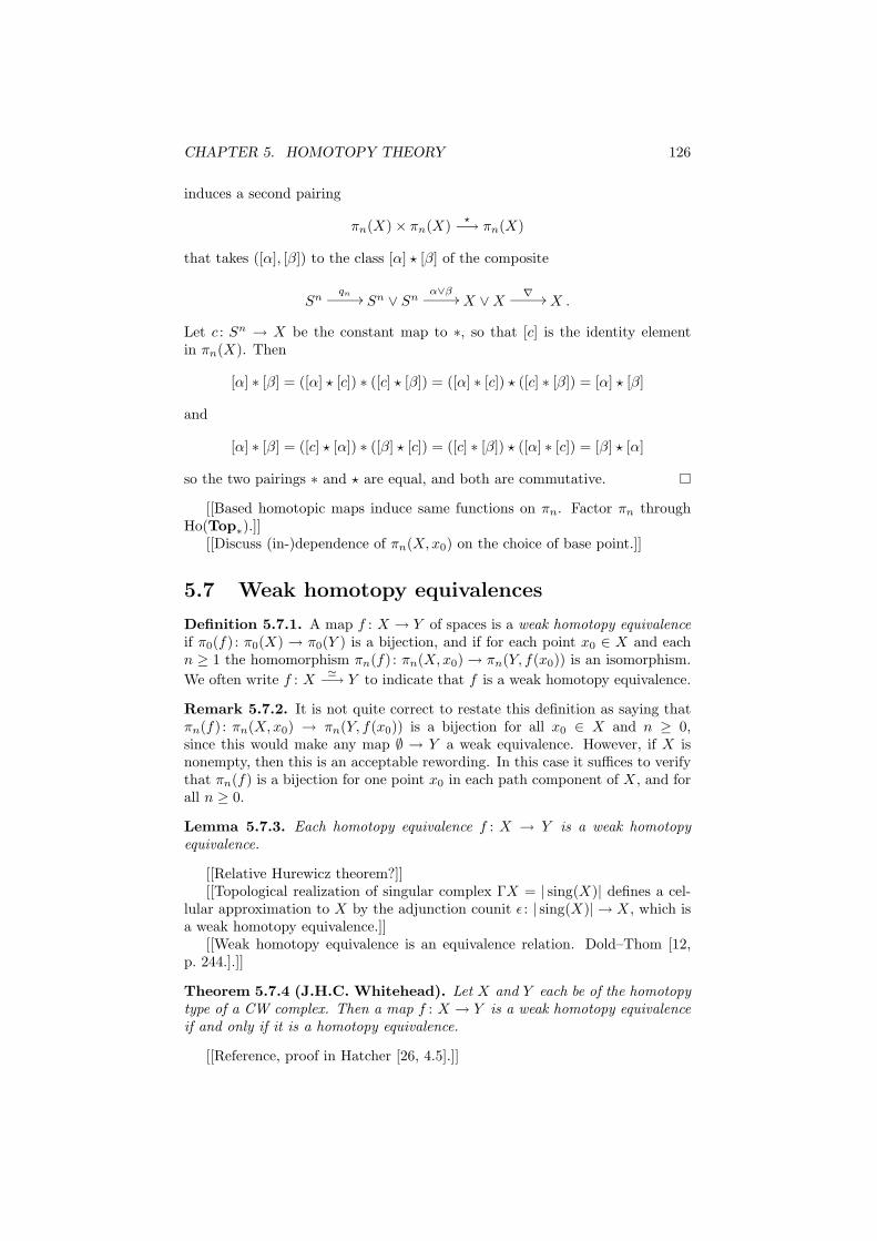
CHAPTER 5. HOMOTOPY THEORY 126
induces a second pairing
πn(X) × πn(X)⋆
−→ πn(X)
that takes ([α], [β]) to the class [α] ⋆ [β] of the composite
Snqn // Sn ∨ Sn
α∨β// X ∨ X
∇ // X .
Let c : Sn → X be the constant map to ∗, so that [c] is the identity elementin πn(X). Then
[α] ∗ [β] = ([α] ⋆ [c]) ∗ ([c] ⋆ [β]) = ([α] ∗ [c]) ⋆ ([c] ∗ [β]) = [α] ⋆ [β]
and
[α] ∗ [β] = ([c] ⋆ [α]) ∗ ([β] ⋆ [c]) = ([c] ∗ [β]) ⋆ ([α] ∗ [c]) = [β] ⋆ [α]
so the two pairings ∗ and ⋆ are equal, and both are commutative.
[[Based homotopic maps induce same functions on πn. Factor πn throughHo(Top∗).]]
[[Discuss (in-)dependence of πn(X,x0) on the choice of base point.]]
5.7 Weak homotopy equivalences
Definition 5.7.1. A map f : X → Y of spaces is a weak homotopy equivalenceif π0(f) : π0(X) → π0(Y ) is a bijection, and if for each point x0 ∈ X and eachn ≥ 1 the homomorphism πn(f) : πn(X,x0) → πn(Y, f(x0)) is an isomorphism.
We often write f : X≃−→ Y to indicate that f is a weak homotopy equivalence.
Remark 5.7.2. It is not quite correct to restate this definition as saying thatπn(f) : πn(X,x0) → πn(Y, f(x0)) is a bijection for all x0 ∈ X and n ≥ 0,since this would make any map ∅ → Y a weak equivalence. However, if X isnonempty, then this is an acceptable rewording. In this case it suffices to verifythat πn(f) is a bijection for one point x0 in each path component of X, and forall n ≥ 0.
Lemma 5.7.3. Each homotopy equivalence f : X → Y is a weak homotopyequivalence.
[[Relative Hurewicz theorem?]][[Topological realization of singular complex ΓX = | sing(X)| defines a cel-
lular approximation to X by the adjunction counit ǫ : | sing(X)| → X, which isa weak homotopy equivalence.]]
[[Weak homotopy equivalence is an equivalence relation. Dold–Thom [12,p. 244.].]]
Theorem 5.7.4 (J.H.C. Whitehead). Let X and Y each be of the homotopytype of a CW complex. Then a map f : X → Y is a weak homotopy equivalenceif and only if it is a homotopy equivalence.
[[Reference, proof in Hatcher [26, 4.5].]]
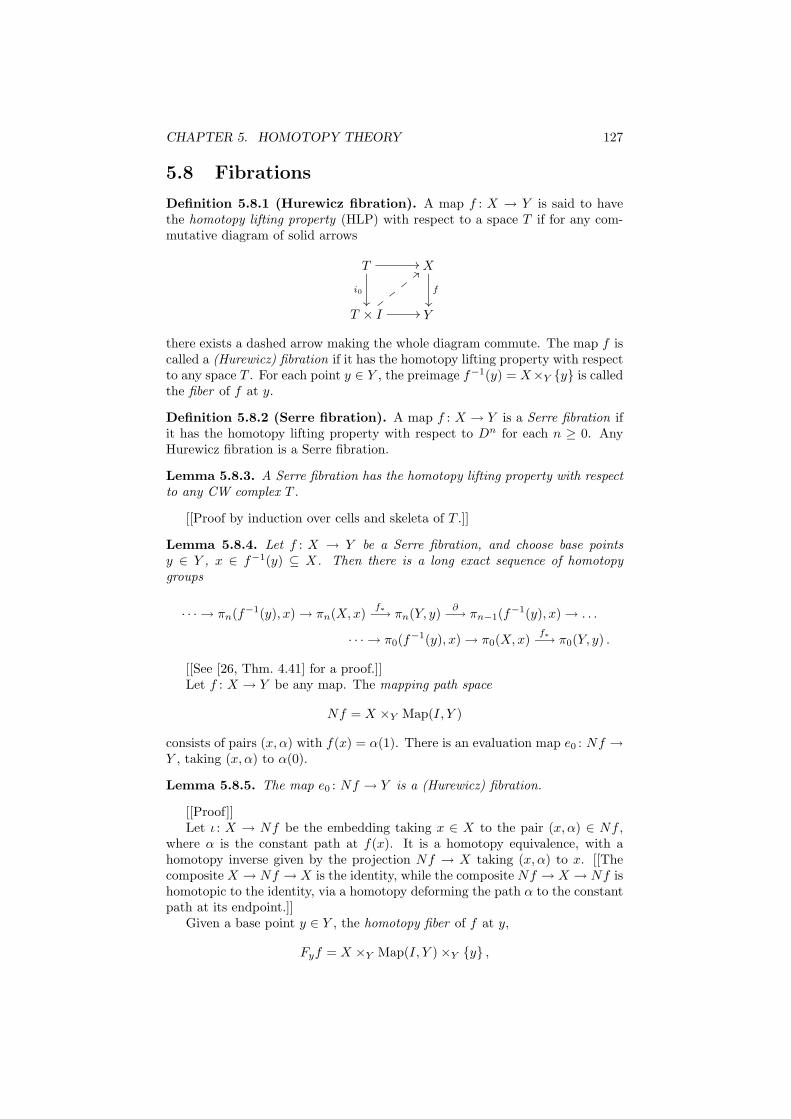
CHAPTER 5. HOMOTOPY THEORY 127
5.8 Fibrations
Definition 5.8.1 (Hurewicz fibration). A map f : X → Y is said to havethe homotopy lifting property (HLP) with respect to a space T if for any com-mutative diagram of solid arrows
T
i0
²²
// X
f
²²
T × I //
<<xx
xx
Y
there exists a dashed arrow making the whole diagram commute. The map f iscalled a (Hurewicz) fibration if it has the homotopy lifting property with respectto any space T . For each point y ∈ Y , the preimage f−1(y) = X×Y y is calledthe fiber of f at y.
Definition 5.8.2 (Serre fibration). A map f : X → Y is a Serre fibration ifit has the homotopy lifting property with respect to Dn for each n ≥ 0. AnyHurewicz fibration is a Serre fibration.
Lemma 5.8.3. A Serre fibration has the homotopy lifting property with respectto any CW complex T .
[[Proof by induction over cells and skeleta of T .]]
Lemma 5.8.4. Let f : X → Y be a Serre fibration, and choose base pointsy ∈ Y , x ∈ f−1(y) ⊆ X. Then there is a long exact sequence of homotopygroups
· · · → πn(f−1(y), x) → πn(X,x)f∗−→ πn(Y, y)
∂−→ πn−1(f
−1(y), x) → . . .
· · · → π0(f−1(y), x) → π0(X,x)
f∗−→ π0(Y, y) .
[[See [26, Thm. 4.41] for a proof.]]Let f : X → Y be any map. The mapping path space
Nf = X ×Y Map(I, Y )
consists of pairs (x, α) with f(x) = α(1). There is an evaluation map e0 : Nf →Y , taking (x, α) to α(0).
Lemma 5.8.5. The map e0 : Nf → Y is a (Hurewicz) fibration.
[[Proof]]Let ι : X → Nf be the embedding taking x ∈ X to the pair (x, α) ∈ Nf ,
where α is the constant path at f(x). It is a homotopy equivalence, with ahomotopy inverse given by the projection Nf → X taking (x, α) to x. [[Thecomposite X → Nf → X is the identity, while the composite Nf → X → Nf ishomotopic to the identity, via a homotopy deforming the path α to the constantpath at its endpoint.]]
Given a base point y ∈ Y , the homotopy fiber of f at y,
Fyf = X ×Y Map(I, Y ) ×Y y ,
CHAPTER 5. HOMOTOPY THEORY 128
equals the fiber of e0 : Nf → Y at y. It consists of pairs (x, α), with x ∈ X andα : I → Y such that α(0) = y and α(1) = f(x). Under the embedding ι, thefiber f−1(y) is identified with a subspace of the homotopy fiber Fyf , and thereis a commutative diagram
f−1(y) //
ι
²²
Xf
//
ι ≃
²²
Y
=
²²Fyf // Nf
e0 // Y .
Lemma 5.8.6. Let f : X → Y be any map, and choose base points y ∈ Y ,x ∈ f−1(y) ⊆ X. Then there is a long exact sequence
· · · → πn(Fyf, ι(x)) → πn(X,x)f∗−→ πn(Y, y)
∂−→ πn−1(Fyf, x) → . . .
· · · → π0(Fyf, ι(x)) → π0(X,x) → π0(Y, y) .
Proof. This is the long exact sequence associated to the (Hurewicz, hence Serre)fibration Fyf → Nf → Y , with πn(X,x) replacing its isomorphic image underι∗, that is πn(Nf, ι(x)).
The following definition is due to Dold, see [12].
Definition 5.8.7 (Quasi-fibration). A map f : X → Y is a quasi-fibration iffor each point y ∈ Y the inclusion
ι : f−1(y)≃−→ Fyf
is a weak homotopy equivalence.
Lemma 5.8.8. Let f : X → Y be a quasi-fibration, and choose base pointsy ∈ Y , x ∈ f−1(y) ⊆ X. Then there is a long exact sequence
· · · → πn(f−1(y), x) → πn(X,x)f∗−→ πn(Y, y)
∂−→ πn−1(f
−1(y), x) → . . .
· · · → π0(f−1(y), x) → π0(X,x) → π0(Y, y) .
Proof. This is the long exact sequence above, with πn(f−1(y), x) replacing itsisomorphic image πn(Fyf, ι(x)).
Lemma 5.8.9. Any Serre fibration f : X → Y is a quasi-fibration.
Proof. Let y ∈ Y . If f−1(y) is empty, then so is Fyf , by the homotopy liftingproperty. Otherwise, for each choice of base point x ∈ f−1(y), the five-lemmaapplied to the diagram
πn+1(X,x)f∗ //
=
²²
πn+1(Y, y)∂ //
=
²²
πn(f−1(y), x) //
²²
πn(X,x)f∗ //
=
²²
πn(Y, y)
=
²²
πn+1(X,x)f∗ // πn+1(Y, y)
∂ // πn(Fyf, ι(x)) // πn(X,x)f∗ // πn(Y, y)
implies that the middle vertical map is an isomorphism. (Some special care isneeded for n = 0, see [12].)
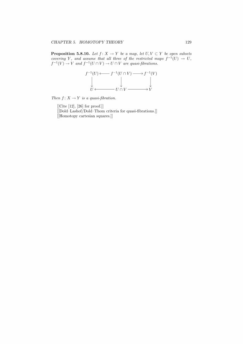
CHAPTER 5. HOMOTOPY THEORY 129
Proposition 5.8.10. Let f : X → Y be a map, let U, V ⊂ Y be open subsetscovering Y , and assume that all three of the restricted maps f−1(U) → U ,f−1(V ) → V and f−1(U ∩ V ) → U ∩ V are quasi-fibrations.
f−1(U)
²²
f−1(U ∩ V )oo //
²²
f−1(V )
²²
U U ∩ Voo // V
Then f : X → Y is a quasi-fibration.
[[Cite [12], [26] for proof.]][[Dold–Lashof/Dold–Thom criteria for quasi-fibrations.]][[Homotopy cartesian squares.]]
Chapter 6
Simplicial methods
6.1 Combinatorial complexes
General references for combinatorial complexes are Eilenberg–Steenrod [17, Ch. 2]and Fritsch–Piccinini [20, Ch. 3].
Definition 6.1.1. For each n ≥ 0, the standard n-simplex ∆n is the convexspan
∆n = (t0, . . . , tn) ∈ Rn+1 |n∑
i=0
ti = 1, ti ≥ 0
of the (n + 1) points
e0 = (1, 0, . . . , 0)
e1 = (0, 1, . . . , 0)
...
en = (0, 0, . . . , 1)
in Rn+1. Note that
(t0, t1, . . . , tn) =
n∑
i=0
tiei .
A Euclidean n-simplex σ in RN is the convex span
σ = n∑
i=0
tivi | (t0, . . . , tn) ∈ ∆n
of (n + 1) points v0, v1, . . . , vn ∈ RN in general position, meaning that the nvectors
v1 − v0 , . . . , vn − v0
are linearly independent. The points v0, v1, . . . , vn are called the vertices of σ.We say that an n-simplex σ has dimension n.
When the total ordering of the vertices is fixed, the presentation of eachpoint in σ as a sum
∑ni=0 tivi is unique, and the numbers (t0, t1, . . . , tn) are
called the barycentric coordinates of the point. A Euclidean simplex τ is a faceof a Euclidean simplex σ if τ is the convex span of a non-empty subset of thevertices of σ. It is a proper face if τ 6= σ.
130
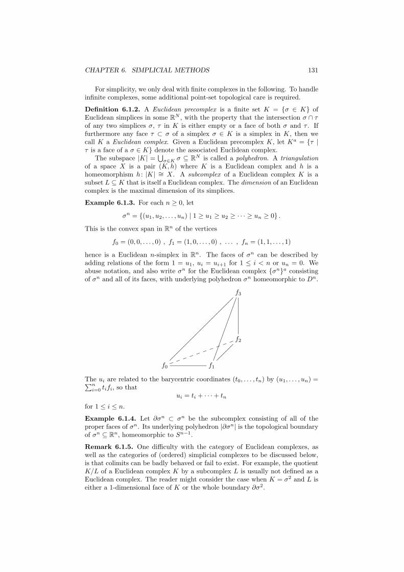
CHAPTER 6. SIMPLICIAL METHODS 131
For simplicity, we only deal with finite complexes in the following. To handleinfinite complexes, some additional point-set topological care is required.
Definition 6.1.2. A Euclidean precomplex is a finite set K = σ ∈ K ofEuclidean simplices in some RN , with the property that the intersection σ ∩ τof any two simplices σ, τ in K is either empty or a face of both σ and τ . Iffurthermore any face τ ⊂ σ of a simplex σ ∈ K is a simplex in K, then wecall K a Euclidean complex. Given a Euclidean precomplex K, let Ka = τ |τ is a face of a σ ∈ K denote the associated Euclidean complex.
The subspace |K| =⋃
σ∈K σ ⊆ RN is called a polyhedron. A triangulationof a space X is a pair (K,h) where K is a Euclidean complex and h is ahomeomorphism h : |K| ∼= X. A subcomplex of a Euclidean complex K is asubset L ⊆ K that is itself a Euclidean complex. The dimension of an Euclideancomplex is the maximal dimension of its simplices.
Example 6.1.3. For each n ≥ 0, let
σn = (u1, u2, . . . , un) | 1 ≥ u1 ≥ u2 ≥ · · · ≥ un ≥ 0 .
This is the convex span in Rn of the vertices
f0 = (0, 0, . . . , 0) , f1 = (1, 0, . . . , 0) , . . . , fn = (1, 1, . . . , 1)
hence is a Euclidean n-simplex in Rn. The faces of σn can be described byadding relations of the form 1 = u1, ui = ui+1 for 1 ≤ i < n or un = 0. Weabuse notation, and also write σn for the Euclidean complex σna consistingof σn and all of its faces, with underlying polyhedron σn homeomorphic to Dn.
f3
f2
f0
ÄÄÄÄÄÄÄÄÄÄÄÄÄÄÄÄÄÄÄÄÄÄÄÄÄÄÄ
jjjjjjjjjjf1
ÄÄÄÄÄÄÄ
¶¶¶¶¶¶¶¶¶¶¶¶¶¶¶¶¶¶¶¶
The ui are related to the barycentric coordinates (t0, . . . , tn) by (u1, . . . , un) =∑ni=0 tifi, so that
ui = ti + · · · + tn
for 1 ≤ i ≤ n.
Example 6.1.4. Let ∂σn ⊂ σn be the subcomplex consisting of all of theproper faces of σn. Its underlying polyhedron |∂σn| is the topological boundaryof σn ⊆ Rn, homeomorphic to Sn−1.
Remark 6.1.5. One difficulty with the category of Euclidean complexes, aswell as the categories of (ordered) simplicial complexes to be discussed below,is that colimits can be badly behaved or fail to exist. For example, the quotientK/L of a Euclidean complex K by a subcomplex L is usually not defined as aEuclidean complex. The reader might consider the case when K = σ2 and L iseither a 1-dimensional face of K or the whole boundary ∂σ2.
CHAPTER 6. SIMPLICIAL METHODS 132
Example 6.1.6. Let Σn act on Rn by permuting the coordinates, with π ∈ Σn
taking (u1, u2, . . . , un) to
π · (u1, u2, . . . , un) = (uπ−1(1), uπ−1(2), . . . , uπ−1(n)) .
The setCn = π(σn) | π ∈ Σn
a
is then a Euclidean complex in Rn. To prove that π1(σn) ∩ π2(σ
n) is a face ofboth π1(σ
n) and π2(σn), for π1, π2 ∈ Σn, it suffices to check that σn∩π(σn) is the
face of σn where uπ(i) = uπ(j) for all i < j with π(i) > π(j), for any π ∈ Σn. Tosee this, note that (u1, . . . , un) ∈ σn has the form π(v1, . . . , vn) ∈ π(σn) only if(v1, . . . , vn) = π−1(u1, . . . , un) = (uπ(1), . . . , uπ(n)), so that uπ(1) ≥ · · · ≥ uπ(n).The underlying polyhedron of Cn is the n-cube
|Cn| =⋃
π∈Σn
π(σn) = In
since any point (w1, . . . , wn) in In has the form π · (u1, . . . , un) for some π ∈ Σn
and (u1, . . . , un) ∈ σn.
Definition 6.1.7. A permutation π ∈ Σm+n is called an (m,n)-shuffle if
π(1) < · · · < π(m) , π(m + 1) < · · · < π(m + n) .
An (m,n)-shuffle π is uniquely determined by the subset π(1), . . . , π(m) of1, . . . ,m+n, so altogether there are precisely (m,n) = (m+n)!/m!n! different(m,n)-shuffles. The inverse of an (m,n)-shuffle is not necessarily an (m,n)-shuffle.
Lemma 6.1.8. The product σm × σn ⊆ Im × In = Im+n is triangulated by theEuclidean complex
Pm,n = π−1(σm+n) | π is an (m,n)-shufflea .
Hence|Pm,n| =
⋃
(m, n)-shuffles π
π−1(σm+n) = σm × σn .
Proof. Pm,n is a subcomplex of Cm+n, hence is a Euclidean complex. Thepolyhedron |Pm,n| consists of the points of the form
(w1, . . . , wm+n) = π−1 · (u1, . . . , um+n) = (uπ(1), . . . , uπ(m+n))
with π an (m,n)-shuffle and 1 ≥ u1 ≥ · · · ≥ um+n ≥ 0, which precisely meansthat 1 ≥ w1 ≥ · · · ≥ wm ≥ 0 and 1 ≥ wm+1 ≥ · · · ≥ wm+n ≥ 0. These areexactly the points in the product σm × σn.
Definition 6.1.9. Let K be a Euclidean complex. Let the n-skeleton
K(n) = σ ∈ K | dim(σ) ≤ n
be the subcomplex of simplices of dimension ≤ n. Let
K♯n = σ ∈ K | dim(σ) = n
be the set of n-simplices in K.
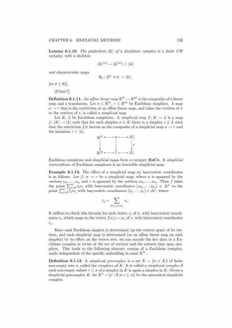
CHAPTER 6. SIMPLICIAL METHODS 133
Lemma 6.1.10. The polyhedron |K| of a Euclidean complex is a finite CWcomplex, with n-skeleton
|K|(n) = |K(n)| ⊂ |K|
and characteristic mapsΦσ : Dn ∼= σ → |K| .
for σ ∈ K♯n.
[[Clear?]]
Definition 6.1.11. An affine linear map RN → RM is the composite of a linearmap and a translation. Let σ ⊂ RN , τ ⊂ RM be Euclidean simplices. A mapσ → τ that is the restriction of an affine linear map, and takes the vertices of σto the vertices of τ , is called a simplicial map.
Let K, L be Euclidean complexes. A simplicial map f : K → L is a mapf : |K| → |L| such that for each simplex σ ∈ K there is a simplex τ ∈ L suchthat the restriction f |σ factors as the composite of a simplicial map σ → τ andthe inclusion τ ⊂ |L|.
RN
²²
σoooo
²²
// // |K|
f
²²
RM τoooo // // |L|
Euclidean complexes and simplicial maps form a category EuCx. A simplicialisomorphism of Euclidean complexes is an invertible simplicial map.
Example 6.1.12. The effect of a simplicial map on barycentric coordinatesis as follows. Let f : σ → τ be a simplicial map, where σ is spanned by thevertices v0, . . . , vm and τ is spanned by the vertices w0, . . . , wn. Then f takesthe point
∑mi=0 uivi with barycentric coordinates (u0, . . . , um) ∈ ∆m to the
point∑n
j=0 tjwj with barycentric coordinates (t0, . . . , tn) ∈ ∆n, where
tj =∑
f(vi)=wj
ui .
It suffices to check this formula for each vertex vi of σ, with barycentric coordi-nates ei, which maps to the vertex f(vi) = wj of τ , with barycentric coordinatesej .
Since each Euclidean simplex is determined (as the convex span) of its ver-tices, and each simplicial map is determined (as an affine linear map on eachsimplex) by its effect on the vertex sets, we can encode the key data in a Eu-clidean complex in terms of the set of vertices and the subsets that span sim-plices. This leads to the following abstract version of a Euclidean complex,made independent of the specific embedding in some RN .
Definition 6.1.13. A simplicial precomplex is a set K = σ ∈ K of finitenon-empty sets σ, called the simplices of K. It is called a simplicial complex ifeach non-empty subset τ ⊂ σ of a simplex in K is again a simplex in K. Given asimplicial precomplex K, let Ka = τ | ∅ 6= τ ⊆ σ be the associated simplicialcomplex.
CHAPTER 6. SIMPLICIAL METHODS 134
For a simplicial complex K, let K0 =⋃
σ∈K σ, so that each simplex is asubset of K0. The elements of K0 are called the vertices of K. A simplex with(n + 1) elements is called an n-simplex. The 0-simplices of K are precisely thesingleton sets v for all vertices v.
A simplicial complex K is finite if the set of simplices K is finite, or equiv-alently, if the set of vertices K0 is finite.
Example 6.1.14. To a Euclidean complex K in RN we can associate a finitesimplicial complex sK, with simplices sσ equal to the sets of vertices v0, . . . , vnof the Euclidean simplices σ in K. The set sK0 ⊂ RN is then the set ofall vertices in all of the Euclidean simplices of K. A non-empty subset sσ =v0, . . . , vn ⊆ sK0 is a simplex in sK if and only if the points v0, . . . , vn arethe vertices of a Euclidean simplex σ in K.
Example 6.1.15. To a finite simplicial complex K we can associate a Euclideancomplex eK. First, enumerate the elements of K0 as (v0, . . . , vN ). Then, to eachsimplex σ ∈ K, viewed as a subset σ ⊆ K0, associate the Euclidean simplexeσ in RN with vertices the fj ∈ RN such that vj ∈ σ. The Euclidean complexeK = eσ | σ ∈ K is the set of all these Euclidean simplices eσ. Note thatall of the vertices f0, . . . , fN are in general position within RN , and that twoEuclidean simplices eσ and eτ in eK, corresponding to simplices σ, τ ∈ K, meetat the Euclidean simplex eσ ∩ eτ = e(σ ∩ τ) corresponding to the intersectionσ ∩ τ ∈ K0, unless that intersection is empty. The resulting Euclidean complexeK is a subcomplex of the Euclidean complex σN , so |eK| ⊆ σN .
[[Define a simplicial map of simplicial complexes, and the associated categorySCx.]]
Remark 6.1.16. Starting with a Euclidean complex K, forming a finite sim-plicial complex sK as above, and then forming a Euclidean complex e(sK),there is a simplicial isomorphism e(sK) ∼= K. Conversely, given a finite simpli-cial complex K, forming the Euclidean complex eK and the simplicial complexs(eK), there is a simplicial isomorphism K ∼= s(eK). These two notions ofcombinatorial complexes are therefore effectively equivalent.
To have well-defined barycentric coordinates in a Euclidean simplex, weneeded to fix a total ordering of its vertices. When considering products K ×Lof simplicial complexes, it is likewise essential to work with ordered simplices.We follow Eilenberg–Steenrod [17, II.8.7].
Definition 6.1.17. An ordered simplicial complex (K,≤) is a simplicial com-plex K = σ ∈ K together with a partial ordering (K0,≤) on its set of vertices,such that
(a) the partial ordering ≤ restricts to a total ordering on each simplex σ ⊆ K0,and
(b) two vertices v0, v1 ∈ K0 are unrelated if v0, v1 is not a simplex in K.
A simplicial map f : (K,≤) → (L,≤) of ordered simplicial complexes is anorder-preserving function f : (K0,≤) → (L0,≤) between the vertex sets, suchthat for each simplex σ ⊆ K0 in K the image f(σ) ⊆ L0 is a simplex in L.[[The rule σ 7→ f(σ) then defines a function f : K → L.]] We write OSCx forthe category of ordered simplicial complexes and simplicial maps.
CHAPTER 6. SIMPLICIAL METHODS 135
Example 6.1.18. Each simplicial complex K can be ordered, by first choosinga total ordering on its vertex set K0, and then defining the partial ordering ≤to agree with the total ordering for pairs v0, v1 with v0, v1 a simplex in K,and otherwise making v0, v1 unrelated.
Example 6.1.19. For each n ≥ 0, let (∆[n],≤) be the ordered simplicial com-plex with vertices ∆[n]0 = [n] = 0 < 1 < · · · < n, given the usual totalordering, and with simplices all non-empty subsets ∅ 6= σ ⊆ [n]. The corre-sponding Euclidean complex is e∆[n] = σn.
Example 6.1.20. For each n ≥ 0, let (∂∆[n],≤) ⊂ (∆[n],≤) be the orderedsimplicial subcomplex with simplices all proper, non-empty subsets ∅ 6= σ ⊂ [n].The corresponding Euclidean complex is e∂∆[n] = ∂σn.
Definition 6.1.21. Let (K,≤) and (L,≤) be ordered simplicial complexes. Theproduct (K × L,≤) has vertex set
(K × L)0 = K0 × L0
with the product partial ordering, so that (v0, w0) ≤ (v1, w1) if and only if v0 ≤v1 in (K0,≤) and w0 ≤ w1 in (L0,≤). A finite, nonempty subset σ ⊆ K0 × L0
is a simplex in K × L if and only if
(a) the restriction of ≤ to σ is a total ordering,
(b) the projection prK(σ) ⊆ K0 is a simplex in K, and
(c) the projection prL(σ) ⊆ L0 is a simplex in L.
Lemma 6.1.22. The product (K×L,≤), with the two projection maps prK : (K×L,≤) → (K,≤) and prL : (K × L,≤) → (L,≤), is the categorical product of(K,≤) and (L,≤) in OSCx.
Proof. Given any ordered simplicial complex (M,≤) and simplicial maps f : M →K and g : M → L, the function (f, g) : M0 → K0 × L0 defines the unique sim-plicial map h : M → K × L with prK(h) = f , prK(h) = g. [[Say more?]]
Example 6.1.23. The product (∆[m]×∆[n],≤) is the ordered simplicial com-plex with vertex set
(∆[m] × ∆[n])0 = [m] × [n]
given the product partial ordering, so that (i, j) ≤ (i′, j′) if and only if i ≤ i′
and j ≤ j′.
(0, 1) // (1, 1) // (2, 1)
(0, 0) //
OO
(1, 0) //
OO
(2, 0)
OO
The simplices of ∆[m]×∆[n] are the finite, nonempty subsets of [m]× [n] thatare totally ordered in the inherited ordering. In other words, the p-simplices arethe linear chains
(i0, j0) < (i1, j1) < · · · < (ip, jp)
in [m]× [n]. Note that the projection of such a p-simplex to ∆[m] is the simplexi0, i1, . . . , ip, and its projection to ∆[n] is the simplex j0, j1, . . . , jp. Even if
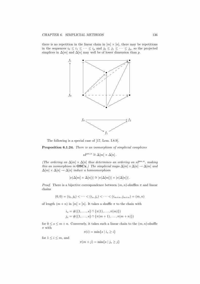
CHAPTER 6. SIMPLICIAL METHODS 136
there is no repetition in the linear chain in [m] × [n], there may be repetitionsin the sequences i0 ≤ i1 ≤ · · · ≤ ip and j0 ≤ j1 ≤ · · · ≤ jp, so the projectedsimplices in ∆[m] and ∆[n] may well be of lower dimension than p.
f1 • //
''NNNNNNNNNNNNNN •
•
77pppppppppppppp
f0
OO
•
OO
>>~~~~~~~~~~~~~~~~~
''NNNNNNNNNNNNNN //_____________
;;ww
ww
ww
ww
ww
ww
ww
ww
•
OO
•
OO
GG²²²²²²²²²²²²²²²²²²²²²²²²²²²²²
77pppppppppppppp
f0//
&&MMMMMMMMMMMMM f2
f1
88qqqqqqqqqqqqq
The following is a special case of [17, Lem. I.8.9].
Proposition 6.1.24. There is an isomorphism of simplicial complexes
sPm,n ∼= ∆[m] × ∆[n] .
(The ordering on ∆[m] × ∆[n] thus determines an ordering on sPm,n, makingthis an isomorphism in OSCx.) The simplicial maps ∆[m]×∆[n] → ∆[m] and∆[m] × ∆[n] → ∆[n] induce a homeomorphism
|e(∆[m] × ∆[n])| ∼= |e(∆[m])| × |e(∆[n])| .
Proof. There is a bijective correspondence between (m,n)-shuffles π and linearchains
(0, 0) = (i0, j0) < · · · < (is, js) < · · · < (im+n, jm+n) = (m,n)
of length (m + n) in [m] × [n]. It takes a shuffle π to the chain with
is = #(1, . . . , s ∩ π(1), . . . , π(m))
js = #(1, . . . , s ∩ π(m + 1), . . . , π(m + n))
for 0 ≤ s ≤ m + n. Conversely, it takes such a linear chain to the (m,n)-shuffleπ with
π(i) = mins | is ≥ i
for 1 ≤ i ≤ m, andπ(m + j) = mins | js ≥ j
CHAPTER 6. SIMPLICIAL METHODS 137
for 1 ≤ j ≤ n. Going up the linear chain, (is, js) = (is−1 + 1, js−1) precisely ifs ∈ π(1), . . . , π(m), and (is, js) = (is−1, js−1 + 1) otherwise.
The isomorphism of simplicial complexes takes (the (m + n)-simplex corre-sponding to) the Euclidean (m+n)-simplex π−1(σm+n) ∈ Pm,n to the (m+n)-simplex
(i0, j0) < · · · < (is, js) < · · · < (im+n, jm+n) (6.1)
in ∆[m]×∆[n], where π and the (is, js) correspond as above. For example, theEuclidean (m + n)-simplex σm+n corresponds to the chain
(0, 0) < (1, 0) < · · · < (m, 0) < (m, 1) < · · · < (m,n) .
A check of definitions shows that two Euclidean (m + n)-simplices π−11 (σm+n)
and π−12 (σm+n) intersect in the face corresponding to intersection of the two
corresponding chains, as required for a simplicial isomorphism. [[Elaborate?]]The projection map ∆[m] × ∆[n] → ∆[m] takes the (m + n)-simplex (6.1)
to the m-simplex 0 < 1 < · · · < m, mapping the elements (is, js) with π(i) ≤s < π(i + 1) to i. (The elements with 0 ≤ s < π(1) map to 0, and the elementswith π(m) ≤ s ≤ m+n map to m.) At the level of polyhedra, it takes the pointwith barycentric coordinates (t0, t1, . . . , tm+n) in the (m + n)-simplex (6.1) tothe point with barycentric coordinates
(t0 + · · · + tπ(1)−1, tπ(1) + · · · + tπ(2)−1, . . . , tπ(m) + · · · + tm+n)
in the m-simplex 0 < 1 < · · · < m. See Example 6.1.12. The resulting map
σm × σn = |Pm,n| ∼= |e(∆[m] × ∆[n])| → |e(∆[m])| = σm
takes a point (w1, . . . , wm+n) = π−1(u1, . . . , um+n) = (uπ(1), . . . , uπ(m+n)) inπ−1(σm+n) ⊂ |Pm,n|, which has barycentric coordinates
(1 − u1, u1 − u2, . . . , um+n) ,
to the point with barycentric coordinates
(1 − uπ(1), uπ(1) − uπ(2), . . . , uπ(m))
in σm, i.e., the point
(uπ(1), . . . , uπ(m)) = (w1, . . . , wm) .
This proves that the composite map σm × σn → σm equals the projection onthe first coordinate, and similarly for the map to σn. Hence the natural map
|e(∆[m] × ∆[n])| → |e(∆[m])| × |e(∆[n])|
is a homeomorphism.
[[It may be simpler to discuss the combinatorics of this isomorphism form = 1, then use induction to get an isomorphism with ∆[1]m × ∆[n], and thenuse that ∆[m] is a retract of ∆[1]m to get the general case.]]
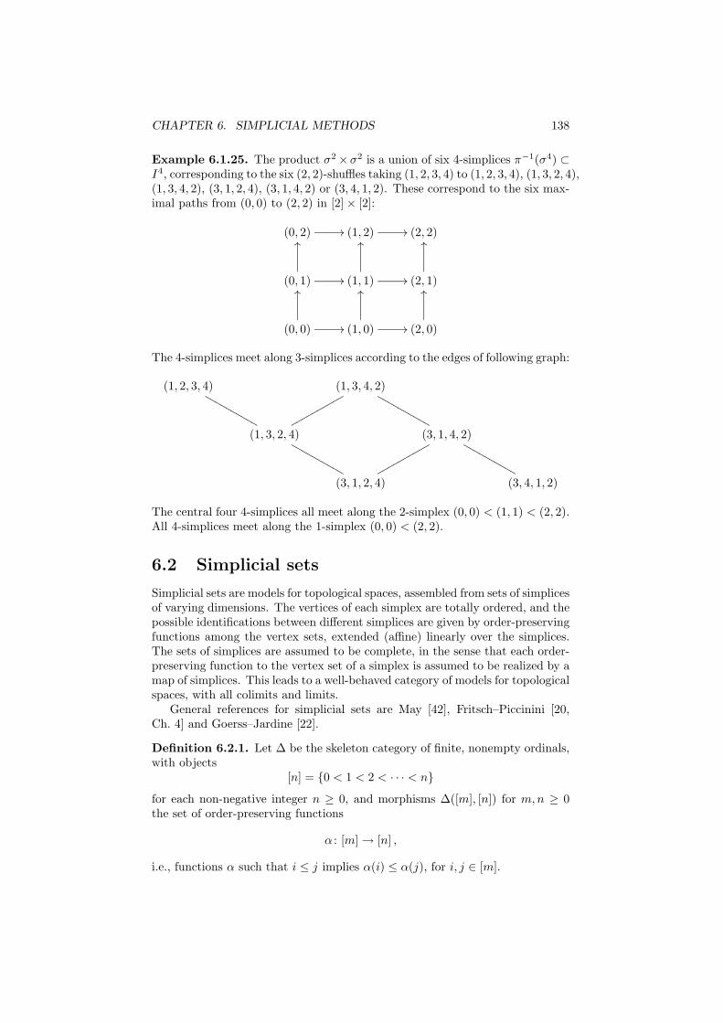
CHAPTER 6. SIMPLICIAL METHODS 138
Example 6.1.25. The product σ2 ×σ2 is a union of six 4-simplices π−1(σ4) ⊂I4, corresponding to the six (2, 2)-shuffles taking (1, 2, 3, 4) to (1, 2, 3, 4), (1, 3, 2, 4),(1, 3, 4, 2), (3, 1, 2, 4), (3, 1, 4, 2) or (3, 4, 1, 2). These correspond to the six max-imal paths from (0, 0) to (2, 2) in [2] × [2]:
(0, 2) // (1, 2) // (2, 2)
(0, 1) //
OO
(1, 1) //
OO
(2, 1)
OO
(0, 0) //
OO
(1, 0) //
OO
(2, 0)
OO
The 4-simplices meet along 3-simplices according to the edges of following graph:
(1, 2, 3, 4)
MMMMMMMMMM(1, 3, 4, 2)
MMMMMMMMMM
(1, 3, 2, 4)
qqqqqqqqqq
MMMMMMMMMM(3, 1, 4, 2)
MMMMMMMMMM
(3, 1, 2, 4)
qqqqqqqqqq(3, 4, 1, 2)
The central four 4-simplices all meet along the 2-simplex (0, 0) < (1, 1) < (2, 2).All 4-simplices meet along the 1-simplex (0, 0) < (2, 2).
6.2 Simplicial sets
Simplicial sets are models for topological spaces, assembled from sets of simplicesof varying dimensions. The vertices of each simplex are totally ordered, and thepossible identifications between different simplices are given by order-preservingfunctions among the vertex sets, extended (affine) linearly over the simplices.The sets of simplices are assumed to be complete, in the sense that each order-preserving function to the vertex set of a simplex is assumed to be realized by amap of simplices. This leads to a well-behaved category of models for topologicalspaces, with all colimits and limits.
General references for simplicial sets are May [42], Fritsch–Piccinini [20,Ch. 4] and Goerss–Jardine [22].
Definition 6.2.1. Let ∆ be the skeleton category of finite, nonempty ordinals,with objects
[n] = 0 < 1 < 2 < · · · < n
for each non-negative integer n ≥ 0, and morphisms ∆([m], [n]) for m,n ≥ 0the set of order-preserving functions
α : [m] → [n] ,
i.e., functions α such that i ≤ j implies α(i) ≤ α(j), for i, j ∈ [m].
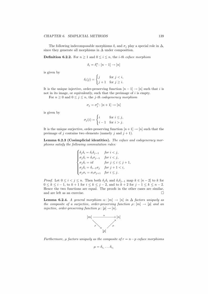
CHAPTER 6. SIMPLICIAL METHODS 139
The following indecomposable morphisms δi and σj play a special role in ∆,since they generate all morphisms in ∆ under composition.
Definition 6.2.2. For n ≥ 1 and 0 ≤ i ≤ n, the i-th coface morphism
δi = δni : [n − 1] → [n]
is given by
δi(j) =
j for j < i,
j + 1 for j ≥ i.
It is the unique injective, order-preserving function [n − 1] → [n] such that i isnot in its image, or equivalently, such that the preimage of i is empty.
For n ≥ 0 and 0 ≤ j ≤ n, the j-th codegeneracy morphism
σj = σnj : [n + 1] → [n]
is given by
σj(i) =
i for i ≤ j,
i − 1 for i > j.
It is the unique surjective, order-preserving function [n+1] → [n] such that thepreimage of j contains two elements (namely j and j + 1).
Lemma 6.2.3 (Cosimplicial identities). The coface and codegeneracy mor-phisms satisfy the following commutation rules:
δjδi = δiδj−1 for i < j,
σjδi = δiσj−1 for i < j,
σjδi = id for j ≤ i ≤ j + 1,
σjδi = δi−1σj for j + 1 < i,
σjσi = σiσj+1 for i ≤ j.
Proof. Let 0 ≤ i < j ≤ n. Then both δjδi and δiδj−1 map k ∈ [n − 2] to k for0 ≤ k ≤ i − 1, to k + 1 for i ≤ k ≤ j − 2, and to k + 2 for j − 1 ≤ k ≤ n − 2.Hence the two functions are equal. The proofs in the other cases are similar,and are left as an exercise.
Lemma 6.2.4. A general morphism α : [m] → [n] in ∆ factors uniquely asthe composite of a surjective, order-preserving function ρ : [m] → [p] and aninjective, order-preserving function µ : [p] → [n].
[m]α //
ρÃÃ
AAAA
AAAA
[n]
[p]
µ
??~~~~~~~
Furthermore, µ factors uniquely as the composite of r = n−p coface morphisms
µ = δir. . . δi1
CHAPTER 6. SIMPLICIAL METHODS 140
subject to the conditions 0 ≤ i1 < · · · < ir ≤ n, and ρ factors uniquely as thecomposite of s = m − p codegeneracy morphisms
ρ = σj1 . . . σjs
subject to the conditions 0 ≤ j1 < · · · < js < m. Hence
α = µρ = δir. . . δi1σj1 . . . σjs
.
Proof. We list the elements in [n] that are in the image of α in increasing order,as
µ(0) < · · · < µ(p)
and this defines the injective morphism µ, with the same image as α. Thesurjective morphism ρ is uniquely determined by the condition α = µρ.
We list the elements in [n] that are not in the image of µ in increasing order,as
i1 < · · · < ir .
Then the composite injective morphism δir. . . δi1 : [p] → [n] has the same image
as µ, hence is equal to µ.We list the elements j in 0, 1, . . . ,m − 1 that have the same image under
ρ as their successor j + 1, in increasing order as
j1 < · · · < js .
Then the composite surjective morphism σj1 . . . σjs: [m] → [p] identifies j and
j + 1 for the same 0 ≤ j < m as ρ, hence is equal to ρ.
Remark 6.2.5. Any finite composable chain of coface and codegeneracy mor-phisms can be brought to the standard form of Lemma 6.2.4, using only thecosimplicial identities. First all codegeneracies can be brought to the right ofall cofaces, using the three expressions for σjδi. Next all cofaces can be broughtin order of descending indices, by replacing δiδj−1 by δjδi whenever j − 1 ≥ i.Finally all codegeneracies can be brought in order of increasing indices, by re-placing σjσi by σiσj+1 whenever j ≥ i.
Definition 6.2.6. A simplicial set X• is a contravariant functor X : ∆op → Setfrom ∆ to sets. For each object [n] in ∆ we write
Xn = X([n])
for the set of n-simplices in X•. For each morphism α : [m] → [n] in ∆ we write
α∗ = X(α) : Xn → Xm
for the associated simplicial operator. In particular, for n ≥ 1 and 0 ≤ i ≤ n,the i-th face operator in X• is the function
di = δ∗i : Xn → Xn−1 ,
and for n ≥ 0 and 0 ≤ j ≤ n, the j-th degeneracy operator in X• is the function
sj = σ∗j : Xn → Xn+1 .
CHAPTER 6. SIMPLICIAL METHODS 141
Lemma 6.2.7 (Simplicial identities). The face and degeneracy operators ina simplicial set X• satisfy the following commutation rules:
didj = dj−1di for i < j,
disj = sj−1di for i < j,
disj = id for j ≤ i ≤ j + 1,
disj = sjdi−1 for j + 1 < i,
sisj = sj+1si for i ≤ j.
Proof. This is clear from Lemma 6.2.3 and the contravariance of X.
The following converse holds.
Lemma 6.2.8. To specify a simplicial set X• it is necessary and sufficient tospecify
(a) a sequence of sets Xn for n ≥ 0,
(b) functions di : Xn → Xn−1 for all 0 ≤ i ≤ n ≥ 1, and
(c) functions sj : Xn → Xn+1 for all 0 ≤ j ≤ n, such that
(d) the di and sj satisfy the simplicial identities.
Proof. For each morphism α : [m] → [n], the simplicial operator α∗ : Xn → Xm
can only be defined as the composite
α∗ = sjs. . . sj1di1 . . . dir
where α = δir. . . δi1σi1 . . . σis
. The main thing to verify is that this specifies awell-defined functor, so that (αβ)∗ = β∗α∗. Since the composite of the standardforms for β and α can be brought to the standard form for αβ using only thecosimplicial identities, and the di and si are assumed to satisfy the simplicialidentities, the two functions (αβ)∗ and β∗α∗ will, indeed, be equal.
Definition 6.2.9. A map of simplicial sets f• : X• → Y• is a natural trans-formation f : X ⇒ Y of functors ∆op → Set. Let sSet be the category ofsimplicial sets and maps, with the obvious notions of identity and composition.
Equivalently, a simplicial map f• amounts to a function
fn : Xn → Yn
for each object [n] in ∆, such that for each morphism α : [m] → [n] in ∆ thesquare
Xnfn //
α∗
²²
Yn
α∗
²²
Xmfm // Ym
commutes. It suffices to verify this condition for the face and degeneracy oper-ators, meaning that difn = fn−1di for 0 ≤ i ≤ n ≥ 1, and sjfn = fn+1sj for0 ≤ j ≤ n, since these operators generate all morphisms in ∆.
We say that X• is a simplicial subset of Y• if each Xn is a subset of Yn, andthe inclusion X• ⊆ Y• is a simplicial map.
CHAPTER 6. SIMPLICIAL METHODS 142
[[This terminology is imprecise, since we are not talking about a simplicialobject in a category of subsets. Saying a “sub simplicial set” might be better,but how to hyphenate this?]]
Lemma 6.2.10. A map f• : X• → Y• of simplicial sets is an isomorphism insSet if and only if each function fn : Xn → Yn is bijective.
A degreewise injective map f• : X• → Y• of simplicial sets induces an iso-morphism of X• with its image f•(X•), as a simplicial subset of Y•.
Proof. The inverse functions gn = f−1n : Yn → Xn define a simplicial map
g• : Y• → X•. If f• is simplicial, then the subsets fn(Xn) ⊆ Yn are closedunder the simplicial operators. Hence the simplicial structure on Y• restricts toa simplicial structure on f•(X•).
Definition 6.2.11. Recall that for each n ≥ 0, the standard n-simplex is theconvex subspace
∆n = (t0, . . . , tn) |n∑
i=0
ti = 1, ti ≥ 0
of Rn+1 spanned by the (n + 1) vertices e0, e1, . . . , en.For each order-preserving function α : [m] → [n], let α∗ : ∆m → ∆n be the
linear map given by α∗(ej) = eα(j) for all 0 ≤ j ≤ m. In formulas,
α∗(
m∑
j=0
ujej) =
m∑
j=0
ujeα(j)
for (u0, u1, . . . , um) ∈ ∆m, or equivalently,
α∗(u0, u1, . . . , um) = (t0, t1, . . . , tn)
whereti =
∑
α(j)=i
uj =∑
j∈α−1(i)
uj .
Example 6.2.12. For each 0 ≤ i ≤ n ≥ 1, δi∗ : ∆n−1 → ∆n is the embedding
δi∗(u0, u1, . . . , un−1) = (u0, . . . , ui−1, 0, ui, . . . , un−1)
onto the face of ∆n where ti = 0, known as the i-th face. It is opposite to thei-th vertex ei, where ti = 1.
We write
∂∆n =n⋃
i=0
δi∗(∆n−1)
for the boundary of ∆n.For each 0 ≤ j ≤ n, σj∗ : ∆n+1 → ∆n is the identification map
σj∗(u0, u1, . . . , un+1) = (u0, . . . , uj−1, uj + uj+1, uj+1, . . . , un+1)
that collapses the edge between ej and ej+1 to one point.
CHAPTER 6. SIMPLICIAL METHODS 143
Lemma 6.2.13. The rules [n] 7→ ∆n, α 7→ α∗ define a (covariant) functor
∆(−) : ∆ −→ Top .
Proof. For α : [m] → [n], β : [n] → [p] the composite β∗α∗ : ∆m → ∆p is given onvertices by β∗α∗(ej) = β∗eα(j) = eβα(j), hence agrees with (βα)∗. The relation(id[n])∗ = id∆n is also clear.
We view simplicial sets as models for topological spaces by way of the fol-lowing construction, which is also known as “geometric realization”.
Definition 6.2.14. Let X• be a simplicial set. The topological realization |X•|is the identification space
|X•| =∐
n≥0
Xn × ∆n/ ∼
where ∼ is the equivalence relation generated by the identifications
(x, α∗(ξ)) ∼ (α∗(x), ξ)
for all α : [m] → [n] in ∆, x ∈ Xn and ξ ∈ ∆m. Here we view (x, α∗(ξ)) ∈ Xn ×∆n as lying in the n-th summand of the coproduct, while (α∗(x), ξ) ∈ Xm×∆m
lies in the m-th summand. The same equivalence relation is generated by theidentifications
(x, δi∗(ξ)) ∼ (di(x), ξ)
for all 0 ≤ i ≤ n ≥ 1, x ∈ Xn and ξ ∈ ∆n−1, and the identifications
(x, σj∗(ξ)) ∼ (sj(x), ξ)
for all 0 ≤ j ≤ n, x ∈ Xn and ξ ∈ ∆n+1.
Remark 6.2.15. Note how each element x ∈ Xn, an “abstract” n-simplex,gives rise to a Euclidean n-simplex x × ∆n in
∐n≥0 Xn × ∆n, that maps to
|X•|.Each point in the boundary ∂∆n ⊂ ∆n of the Euclidean n-simplex lies in
some face, say the i-th, and can then be written as δi∗(ξ) for some ξ ∈ ∆n−1.The relation (x, δi∗(ξ)) ∼ (di(x), ξ) tells us that that boundary point of thex’th Euclidean n-simplex is identified with a point in the Euclidean (n − 1)-simplex di(x) × ∆n−1 associated to the abstract (n − 1)-simplex di(x). Theface operators di : Xn → Xn−1 therefore specify how the boundary faces of eachn-simplex are to be identified as (n − 1)-simplices.
Some abstract n-simplices are of the form sj(x), for 0 ≤ j ≤ n. Herex ∈ Xn−1, and n ≥ 1. The corresponding Euclidean n-simplex sj(x) × ∆n
is then identified with the Euclidean (n − 1)-simplex x × ∆n−1 associated tox, via the map σj∗ : ∆n → ∆n−1 that collapses the edge from ej to ej+1 to apoint. These Euclidean n-simplices sj(x) × ∆n do therefore not contributeany new points to |X•|.
Lemma 6.2.16. Let f• : X• → Y• be any map of simplicial sets. The maps
∐
n≥0
fn × id :∐
n≥0
Xn × ∆n −→∐
n≥0
Yn × ∆n
CHAPTER 6. SIMPLICIAL METHODS 144
descend to a unique map|f•| : |X•| −→ |Y•| .
The rules X• 7→ |X•|, f• 7→ |f•| define the topological realization functor
| − | : sSet −→ Top .
Proof. For each identification (x, α∗(ξ)) ∼ (α∗(x), ξ) made in |X•|, we have theidentification
(fn(x), α∗(ξ)) ∼ (α∗(fn(x)), ξ) = (fm(α∗(x)), ξ)
between the image points, made in |Y•|, so |f•| is well-defined. Given a secondmap g• : Y• → Z• of simplicial sets, the maps |g•f•| and |g•||f•| are both inducedby ∐
n≥0
gnfn × id = (∐
n≥0
gn × id) (∐
n≥0
fn × id) ,
hence are equal.
Remark 6.2.17. We shall later show that |X•| is a CW complex and that|f•| is a cellular map. We may then think of | − | as a functor to CW. Thisaffects our interpretation of the topology of products like |X•| × |Y•|, since inCW we use the weak (compactly generated) topology on this product, ratherthan the cartesian product topology. [[If we replace Top by U , this makes nodifference.]]
Definition 6.2.18. Let Y be any topological space. The singular simplicial setsing(Y )• is the simplicial set with n-simplices
sing(Y )n = Top(∆n, Y )
the set of maps σ : ∆n → Y , and with simplicial operators
α∗ = Top(α∗, Y ) : sing(Y )n → sing(Y )m
for all α : [m] → [n] in ∆, taking a singular n-simplex σ : ∆n → Y to thecomposite α∗(σ) = σ α∗ : ∆m → Y .
For example, di(σ) = σ δi∗ is the restriction of σ to the i-th face of∆n, composed with the identification of that face with ∆n−1. It is clear thatsing(Y ) : ∆op → Set is a (contravariant) functor, since (βα)∗(σ) = σβα =α∗β∗(σ) for all composable α, β and σ.
Lemma 6.2.19. Let f : X → Y be any map of topological spaces. The functionsfn : sing(X)n → sing(Y )n, that take σ : ∆n → X to fn(σ) = fσ : ∆n → Y ,define a simplicial map
f• : sing(X)• −→ sing(Y )• .
The rules X 7→ sing(X)•, f 7→ f∗ define a functor
sing : Top −→ sSet .
CHAPTER 6. SIMPLICIAL METHODS 145
Proof. To define a simplicial map, the functions fn for n ≥ 0 must satisfyα∗fn = fmα∗ for all α : [m] → [n], but for each σ : ∆n → X we have α∗(fn(σ)) =fσα∗ = fm(α∗(σ)), so this is clear.
∆mα∗ // ∆n σ // X
f// Y
Given a second map g : Y → Z, it is clear that (gf)• = g•f•, since (gf)n(σ) =gfσ = gn(fn(σ)) for all n ≥ 0 and σ : ∆n → X. Also (idX)• = idsing(X)• isclear.
These two constructions are adjoint.
Proposition 6.2.20. There is natural bijection
Top(|X•|, Y ) ∼= sSet(X•, sing(Y )•) ,
making topological realization left adjoint to the singular simplicial set functor.
sSet|−|
//Top
sing(−)•
oo
Proof. Each map f : |X•| → Y corresponds to maps fn : Xn × ∆n → Y forall n ≥ 0, compatible for all morphisms α in ∆, which in turn correspond tofunctions gn : Xn → Top(∆n, Y ) = sing(Y )n for all n ≥ 0, satisfying similarcompatibilities. This is the same as a map g• : X• → sing(Y )• of simplicialsets.
All small colimits and limits of simplicial sets exist, and are constructeddegreewise.
Lemma 6.2.21. Let X• : C → sSet be a C -shaped diagram of simplicial sets,with C small. The colimit Y• = colimC X• exists, with n-simplices
Yn = colimC
Xn .
Dually, the limit Z• = limC X• exists, with n-simplices
Zn = limC
Xn .
Proof. For each α : [m] → [n] in ∆, the functions
α∗c : Xn(c) → Xm(c)
for objects c in C define a natural transformation α∗ : Xn ⇒ Xm of functorsC → Set, and induce a function of colimits
α∗ : Yn = colimc∈C
Xn(c) −→ colimc∈C
Xm(c) = Ym .
It is straightforward to check that this makes Y• a simplicial set, with theuniversal property of the colimit.
The limit case is dual.
CHAPTER 6. SIMPLICIAL METHODS 146
Corollary 6.2.22. The topological realization functor | − | : sSet → Top com-mutes with all small colimits:
colimc∈C
|X•(c)| ∼= | colimc∈C
X•(c)|
Proof. This is clear from Propositions 4.3.36 and 6.2.20.
Definition 6.2.23. A based simplicial set is a pair (X•, x0), where X• is asimplicial set and x0 ∈ X0 is a chosen 0-simplex. For each n ≥ 0 the set ofn-simplices is then viewed as based at sn
0 (x0) ∈ Xn, where σn0 : [n] → [0] is
the unique morphism and sn0 = (σn
0 )∗. A based simplicial map f• : (X•, x0) →(Y•, y0) is a simplicial map f• such that f0(x0) = y0. Note that fn(sn
0 (x0)) =sn0 (y0) for all n ≥ 0. These objects and morphisms define a category sSet∗.
The topological realization |X•| is based at the image of x0 × ∆0, alsodenoted x0. It defines a functor sSet∗ → Top∗. The smash product X• ∧ Y• isgiven in simplicial degree n by
(X• ∧ Y•)n = Xn ∧ Yn
and there is a canonical simplicial isomorphism (X•×Y•)/(X•∨Y•) ∼= (X•∧Y•).
Definition 6.2.24. Let (−)op : ∆ → ∆ be the (covariant) functor reversingthe total ordering of the objects, taking [n] to [n], but taking α : [m] → [n] toαop : [m] → [n] given by
αop(i) = n − α(m − i)
for i ∈ [m]. For example, δopi = δn−i : [n−1] → [n] and σop
j = σopn−j : [n+1] → [n].
The composite (−)op (−)op is the identity.For a simplicial set X•, given by a functor X : ∆op → Set, let the opposite
simplicial set Xop• be given by the composite functor
X ((−)op)op : ∆op −→ ∆op −→ X .
It takes [n] to Xopn = Xn on objects, but takes α : [m] → [n] to (αop)∗ : Xn →
Xm on morphisms. Hence the i-th face operator dopi : Xop
n → Xopn−1 equals
dn−i : Xn → Xn−1, and the j-th degeneracy operator sopj : Xop
n → Xopn+1 equals
sn−j : Xn → Xn+1.
Lemma 6.2.25. There is a natural cellular homeomorphism
o : |Xop• | ∼= |X•|
such that the composite o2 : |(Xop• )op| ∼= |Xop
• | ∼= |X•| is the identity.
Proof. Let on : ∆n → ∆n be the homeomorphism reversing the order of thebarycentric coordinates, taking (t0, t1, . . . , tn) to (tn, . . . , t1, t0). It takes thei-th vertex ei to the (n − i)-th vertex en−i. The maps
∐
n≥0
id × on :∐
n≥0
Xopn × ∆n −→
∐
n≥0
Xn × ∆n ,
taking (x, ξ) ∈ Xn × ∆n = Xopn × ∆n to (x, on(ξ)) ∈ Xn × ∆, descend to a
unique mapo : |Xop
• | −→ |X•|
since αop∗ om = on α∗ : ∆m → ∆n. [[Elaborate?]] Clearly o2 = id, so o is a
homeomorphism.
CHAPTER 6. SIMPLICIAL METHODS 147
6.3 The role of non-degenerate simplices
Example 6.3.1. Let (K,≤) be an ordered simplicial complex. There is anassociated simplicial set X•, with n-simplices the linear chains
x = (v0 ≤ v1 ≤ · · · ≤ vn)
in the partially ordered vertex set (K0,≤), such that v0, v1, . . . , vn is a simplexin K, necessarily of dimension less than or equal to n. In particular, X0 = K0.For each morphism α : [m] → [n], the function α∗ : Xn → Xm maps an n-simplexx as above to the m-simplex
α∗(x) = (vα(0) ≤ vα(1) ≤ · · · ≤ vα(m)) .
For example, when α = δi : [n − 1] → [n], the face operator di : Xn → Xn−1
omits the i-th vertex vi in the linear chain defining x ∈ Xn.
di(x) = (v0 ≤ · · · ≤ vi−1 ≤ vi+1 ≤ · · · ≤ vn)
When α = σj : [n + 1] → [n] the degeneracy operator sj : Xn → Xn+1 repeatsthe j-th vertex vj in the linear chain.
sj(x) = (v0 ≤ · · · ≤ vj−1 ≤ vj = vj ≤ vj+1 ≤ · · · ≤ vn)
Let (K,≤), (L,≤) be ordered simplicial complexes with associated simplicialsets X• and Y•, and let f : (K,≤) → (L,≤) be a simplicial map of ordered sim-plicial complexes, given by the order-preserving function f : (K0,≤) → (L0,≤).There is an associated map of simplicial sets f• : X• → Y•, with componentsfn : Xn → Yn taking an n-simplex x as above to the n-simplex
fn(x) = (f(v0) ≤ f(v1) ≤ · · · ≤ f(vn)) .
We therefore have a functor
OSCx −→ sSet .
[[Explain why |X•| is homeomorphic to the underlying polyhedron |eK| ofan associated Euclidean complex?]]
Remark 6.3.2. An n-simplex σ ⊆ K0 in an ordered simplicial set is determinedby its (n + 1) vertices, since σ = v ∈ σ. A simplex x ∈ Xn of a simplicial setalso has vertices, namely the elements vi = ǫ∗i (x) ∈ X0 for 0 ≤ i ≤ n, whereǫi : [0] → [n] is given by ǫi(0) = i. However, these (n + 1) elements do not needto be distinct. Furthermore, the n-simplex X is not necessarily determined byits vertices (v0, . . . , vn). We can identify OSCx with the full subcategory ofsSet generated by the simplicial sets X such that each simplex x is uniquelydetermined by its set of vertices ǫ∗i (x)i. [[Elaborate?]] [[If each non-degeneraten-simplex has (n + 1) distinct vertices, we say that X is non-singular.]]
Definition 6.3.3. For each n ≥ 0, let the simplicial n-simplex ∆n• be the
contravariant functor ∆(−, [n]) = Y[n] : ∆op → Set represented by the object[n] in ∆. It has p-simplices
∆np = ∆([p], [n]) = all order-preserving functions ζ : [p] → [n]
CHAPTER 6. SIMPLICIAL METHODS 148
and simplicial structure maps
β∗ : ∆np → ∆n
q
taking ζ : [p] → [n] to β∗(ζ) = ζ β : [q] → [n], for each morphism β : [q] → [p]in ∆.
For each morphism α : [m] → [n] in ∆, there is a map of simplicial sets
α• : ∆m• −→ ∆n
• ,
which on p-simplices is given by the function
∆([p], α) : ∆([p], [m]) −→ ∆([p], [n])
taking ζ : [p] → [m] to α ζ : [p] → [n].
Lemma 6.3.4. For each n ≥ 0 there is a natural bijective correspondence
sSet(∆n• ,X•)
∼=−→ Xn
taking a simplicial map f : ∆n• → X• to the n-simplex fn(id[n]) ∈ Xn. Here
id[n] ∈ ∆nn. The inverse takes an n-simplex x ∈ Xn to the characteristic map
x• : ∆n• → X• ,
given in simplicial degree p by xp(ζ) = ζ∗(x) for ζ : [p] → [n] in ∆np .
Proof. It is clear that x• is simplicial, and that the two constructions are mu-tually inverse.
[[Could have discussed Yoneda embedding Y : C → Fun(C op,Set) earlier,specializing to ∆ → sSet in this case.]]
Remark 6.3.5. This notation is consistent with the notation α• : ∆m• → ∆n
•
for the simplicial map induced by a morphism α : [m] → [n] in ∆, when viewedas a simplex α ∈ ∆n
m.
Lemma 6.3.6. The simplicial set associated to the ordered simplicial complex(∆[n],≤) is (isomorphic to) the simplicial n-simplex ∆n
• .
Proof. Recall from Example 6.1.19 that the vertex set of ∆[n] is the totallyordered set ([n],≤), so the p-simplices of the associated simplicial set are thelinear chains
(z0 ≤ z1 ≤ · · · ≤ zp)
in [n], which we can identify with the order-preserving functions ζ : [p] → [n],with values ζ(i) = zi. By definition, α∗ takes the linear chain to
(ζα(0) ≤ ζα(1) ≤ · · · ≤ ζα(q)) ,
which is identified with the composite function ζ α = α∗(ζ). Hence the twosimplicial sets are isomorphic.
Lemma 6.3.7. The rules [n] 7→ ∆n• , α 7→ α• define a (covariant) functor
∆(−)• : ∆ −→ sSet .
CHAPTER 6. SIMPLICIAL METHODS 149
Proof. It is clear that (βα)• = β•α•.
Lemma 6.3.8. There is a natural homeomorphism |∆(−)• | ∼= ∆(−) of functors
∆ → Top. In other words, there is a homeomorphism
|∆n• |
∼= ∆n
for each n ≥ 0, such that |α•| : |∆m• | → |∆n
• | corresponds to α∗ : ∆m → ∆n, forall α : [m] → [n] in ∆.
Proof. The map ∐
p≥0
∆np × ∆p −→ ∆n
taking (ζ, ξ) ∈ ∆np ×∆p to ζ∗(ξ) ∈ ∆n sends both (α∗(ζ), ξ) and (ζ, α∗(ξ)) to the
same point, hence induces a map |∆n• | −→ ∆n. An inverse map takes ξ ∈ ∆n
to the image of (id[n], ξ) ∈ ∆nn × ∆n. One composite takes ξ to id[n]∗(ξ) = ξ.
The other composite takes the equivalence class of (ζ, ξ) in |∆n• | to the class of
(id[n], ζ∗(ξ)), but these are the same, since ζ∗(id[n]) = ζ. Hence the two mapsare mutually inverse homeomorphisms.
To check naturality with respect to α : [m] → [n], note that (ζ, ξ) ∈ ∆mp ×∆p
corresponds to ζ∗(ξ) ∈ ∆m, which maps to α∗(ζ∗(ξ)) in ∆n. On the other hand,(ζ, ξ) maps to (αζ, ξ) ∈ ∆n
p × ∆p, which corresponds to (αζ)∗(ξ) in ∆m. Thesepoints are equal.
Definition 6.3.9. For each n ≥ 0 the simplicial boundary (n − 1)-sphere ∂∆n•
is the simplicial subset of ∆n• with p-simplices
∂∆np = ζ ∈ ∆n
p | ζ : [p] → [n] is not surjective
the set of order-preserving functions ζ : [p] → [n] with ζ([p]) 6= [n], i.e., thenon-surjective order-preserving functions.
Lemma 6.3.10. The simplicial set associated to the ordered simplicial complex(∂∆[n],≤) is (isomorphic to) the simplicial boundary (n − 1)-sphere ∂∆n
• .
Proof. The p-simplices of the associated simplicial set are the linear chains
(z0 ≤ z1 ≤ · · · ≤ zp)
in [n] such that z0, z1, . . . , zp are the vertices of a simplex in ∂∆[n], which isequivalent to asking that z0, z1, . . . , zp is a (non-empty) proper subset of [n],which in turn is equivalent to the condition that the order-preserving functionζ : [p] → [n] with ζ(i) = zi is not surjective.
Lemma 6.3.11. The inclusion ∂∆n• ⊂ ∆n
• induces the embedding ∂∆n ⊂ ∆n
upon topological realization.
Proof. Let C be the subcategory of the overcategory ∆/[n], consisting of pairs(p, µ) where µ : [p] → [n] in ∆ is injective but not the identity. We can identifyit with the partially ordered set of proper, non-empty subsets ∅ 6= S ⊂ [n], bytaking µ to its image. In this way is also corresponds to the category of properfaces of ∆n.
CHAPTER 6. SIMPLICIAL METHODS 150
Let F : C → sSet be the functor F ([p], µ) = ∆p•, taking a morphism
β : [q] → [p] from (q, βµ) to (p, µ), to the simplicial map β• : ∆q• → ∆p
•. Thenthe compatible maps j(p,µ) = µ• : ∆p
• → ∆n• induce a map
colimC
F = colim(p,µ)∈C
∆p• −→ ∆n
• ,
which identifies the colimit with ∂∆n• inside of the target. This can be checked
degreewise, as an identity of sets. By Corollary 6.2.22, we get a homeomorphism
colim(p,µ)∈C
∆p = colim(p,µ)∈C
|∆p•|
∼= | colim(p,µ)∈C
∆p•|
∼= |∂∆n• |
and it is clear that colim(p,µ)∈C ∆p = ∂∆n.
Exercise 6.3.12. Enumerate the n-simplices of ∆1• as
∆1n = ζn
0 , . . . , ζnn+1
where ζnk : [n] → [1] maps 0, . . . , k − 1 to 0 and k, . . . , n to 1, for 0 ≤ k ≤
n + 1. Show that
di(ζnk ) =
ζn−1k−1 for 0 ≤ i < k
ζn−1k for k ≤ i ≤ n
for n ≥ 1, and
sj(ζnk ) =
ζn+1k+1 for 0 ≤ j < k
ζn+1k for k ≤ j ≤ n
for n ≥ 0. Show that the nondegenerate simplices of ∆1• (see Definition 6.3.15)
are ζ00 , ζ0
1 and ζ11 .
With notation as above, the n-simplices of ∂∆1• are
∂∆1n = ζn
0 , ζnn+1 .
Enumerate the n-simplices of S1• = ∆1
•/∂∆1• as
S1n = ζn
0 , . . . , ζnn ,
where now ζn0 = ζn
n+1. Obtain formulas for di(ζnk ) and sj(ζ
nk ) in S1
• , for all 0 ≤
i, j, k ≤ n. Note in particular that dn(ζnn ) = ζn−1
0 . What are the nondegeneratesimplices of S1
•?[[Relate S1
• to the Hochschild complex of a ring R.]]
Remark 6.3.13. We can identify ∆1n∼= [n + 1] as sets, taking ζn
k ∈ ∆1n to
k ∈ [n + 1]. Then di : ∆1n → ∆1
n−1 corresponds to σi : [n + 1] → [n] in ∆, andsj : ∆1
n → ∆1n+1 corresponds to δj+1 : [n+1] → [n+2]. We get a (contravariant)
functor ∆1 : ∆op → ∆ ⊂ Set, taking [n] to [n + 1].
Remark 6.3.14. We have at least three useful simplicial models for the topo-logical n-sphere Sn. One is the simplicial boundary n-sphere ∂∆n+1
• with|∂∆n+1
• | ∼= ∂∆n+1. This is the source of the attaching map of (n + 1)-cellsin the CW structure on the topological realization of a simplicial set.
Another is the quotient n-sphere ∆n•/∂∆n
• with |∆n•/∂∆n
• |∼= ∆n/∂∆n. This
is the minimal model for Sn as a based space, and can be used in the descriptionof simplicial homotopy groups.
CHAPTER 6. SIMPLICIAL METHODS 151
A third is the n-fold smash product S1• ∧ · · · ∧S1
• where S1• = ∆1
•/∂∆1•, with
|S1• ∧ · · · ∧ S1
• | = ∆1/∂∆1 ∧ · · · ∧ ∆1/∂∆1. This model has a natural action byΣn, permuting the order of the n smash factors, and appears in the definitionof symmetric spectra.
Definition 6.3.15. Let X• be a simplicial set. An n-simplex x ∈ Xn is saidto be degenerate if x = sj(y) for some (n − 1)-simplex y ∈ Xn−1 and somedegeneracy operator sj : Xn−1 → Xn, for 0 ≤ j < n. Otherwise, x is said to benon-degenerate. Let
sXn =⋃
0≤j<n
sj(Xn−1) ⊆ Xn
be the set of degenerate n-simplices, and let X♯n = Xn \ sXn be the set of
non-degenerate n-simplices.
Example 6.3.16. Let X• be the simplicial set associated to an ordered sim-plicial complex (K,≤). An n-simplex x = (v0 ≤ · · · ≤ vn) is non-degenerateif and only if vj 6= vj+1 for all 0 ≤ j < n, or equivalently, if σ = v0, . . . , vnhas (n + 1) distinct elements, so that σ is an n-simplex in K. Conversely, anyn-simplex σ = v0, . . . , vn in K can be totally ordered as x = (v0 ≤ · · · ≤ vn),and thus determines a non-degenerate n-simplex in X•. We get a one-to-onecorrespondence
K♯n∼= X♯
n
between the n-simplices of (K,≤) and the non-degenerate n-simplices of X•.
We shall prove that |X•| is a CW complex with one n-cell for each non-degenerate n-simplex in X•. The key fact is the following Eilenberg–Zilberlemma from [18, (8.3)], see also [20, Thm. 4.2.3].
Proposition 6.3.17 (Eilenberg–Zilber). Let X• be a simplicial set, and x ∈Xm any m-simplex. There exists a surjective morphism ρ : [m] → [p] and anon-degenerate p-simplex y ∈ Xp such that x = ρ∗(y). Moreover, the pair (ρ, y)is uniquely determined by x.
Proof. The existence part follows easily by induction on m: If x is non-degenerate,we can let ρ = id[m] and y = x. Otherwise x = sj(x1) for some (m− 1)-simplexx1. By induction on m we may assume that x1 = ρ∗1(y) for some surjectiveρ1 : [m − 1] → [p] and y ∈ Xp non-degenerate. Then ρ = ρ1σj : [m] → [p] issurjective and x = ρ∗(y) = (ρ1σj)
∗(y), as required.Suppose that x = ρ∗(y) = τ∗(z) for non-degenerate simplices y ∈ Xp, z ∈ Xq
and surjective morphisms ρ : [m] → [p], τ : [m] → [q]. We must show that y = zand ρ = τ .
x ∈ Xm
µ∗
²²
y ∈ Xp
ρ∗99ssssssssss
=// y ∈ Xp Xq ∋ z
τ∗
eeKKKKKKKKK
(τµ)∗oo
Consider any section µ : [p] → [m] to ρ, with ρµ = id. We get
y = µ∗ρ∗(y) = µ∗τ∗(z) = (τµ)∗(z) .
CHAPTER 6. SIMPLICIAL METHODS 152
We can factor τµ as a composite
τµ = δir. . . δi1σj1 . . . σjs
as in Lemma 6.2.4, so that
(τµ)∗(z) = sjs. . . sj1di1 . . . dir
(z) .
Since y = (τµ)∗(z) is non-degenerate, we must have s = 0, so that τµ : [p] → [q]is injective. Hence p ≤ q. By symmetry, q ≤ p, so p = q. For τµ : [p] → [p]to be order-preserving and injective, it must be the identity, so τµ = id andµ is also a section to τ . Hence y = (τµ)∗(z) = z, proving the uniqueness ofthe non-degenerate y. Two order-preserving surjections ρ, τ : [m] → [p] have thesame set of sections µ : [p] → [m] if and only if they are equal [[Exercise!]], henceρ = τ , proving the uniqueness of the order-preserving surjection ρ.
Corollary 6.3.18. The set of m-simplices of a simplicial set X• decomposesas
Xm∼=
∐
p≥0
X♯p × (∆p
m \ ∂∆pm) ,
with x ∈ Xm corresponding to the unique pair (y, ρ) with x = ρ∗(y), ρ : [m] → [p]surjective (and order-preserving), and y ∈ Xp non-degenerate.
Definition 6.3.19. Given a simplicial set X•, and a set S of simplices in X•,let the simplicial subset of X• generated by S,
〈S〉• ⊆ X• ,
be the minimal simplicial subset of X• that contains all the elements of S. Ithas m-simplices
〈S〉m = α∗(y) ∈ Xm | α ∈ ∆([m], [n]), y ∈ Sn ,
where Sn = S ∩ Xn is the set of n-simplices in S.
Definition 6.3.20. Let the simplicial n-skeleton X(n)• ⊆ X• be the simplicial
subset generated by the set S =⋃
p≤n Xp of simplices of dimension ≤ n in X•.There are natural inclusions
∅ = X(−1)• ⊆ X
(0)• ⊆ · · · ⊆ X
(n−1)• ⊆ X
(n)• ⊆ . . .
with⋃
n≥0 X(n)• = X•, called the simplicial skeleton filtration of X•.
Example 6.3.21. The simplicial boundary (n − 1)-sphere ∂∆n• is the (n − 1)-
skeleton of the simplicial n-simplex ∆n• .
Lemma 6.3.22. The set of m-simplices of X(n)• decomposes as
X(n)m
∼=∐
0≤p≤n
X♯p × (∆p
m \ ∂∆pm) ,
with x ∈ X(n)m corresponding to the unique pair (y, ρ) with x = ρ∗(y), ρ : [m] →
[p] surjective and y ∈ X♯p non-degenerate in X•, with 0 ≤ p ≤ n.
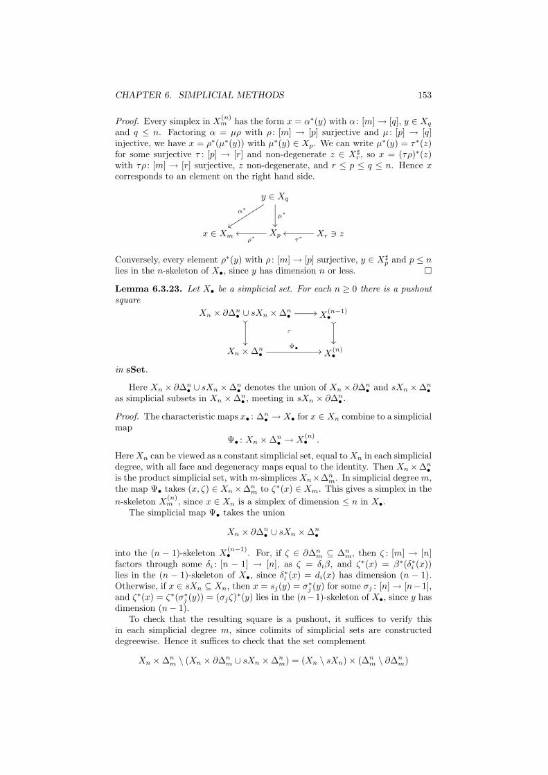
CHAPTER 6. SIMPLICIAL METHODS 153
Proof. Every simplex in X(n)m has the form x = α∗(y) with α : [m] → [q], y ∈ Xq
and q ≤ n. Factoring α = µρ with ρ : [m] → [p] surjective and µ : [p] → [q]injective, we have x = ρ∗(µ∗(y)) with µ∗(y) ∈ Xp. We can write µ∗(y) = τ∗(z)for some surjective τ : [p] → [r] and non-degenerate z ∈ X♯
r, so x = (τρ)∗(z)with τρ : [m] → [r] surjective, z non-degenerate, and r ≤ p ≤ q ≤ n. Hence xcorresponds to an element on the right hand side.
y ∈ Xq
µ∗
²²
α∗
yytttttttttt
x ∈ Xm Xpρ∗
oo Xr ∋ zτ∗
oo
Conversely, every element ρ∗(y) with ρ : [m] → [p] surjective, y ∈ X♯p and p ≤ n
lies in the n-skeleton of X•, since y has dimension n or less.
Lemma 6.3.23. Let X• be a simplicial set. For each n ≥ 0 there is a pushoutsquare
Xn × ∂∆n• ∪ sXn × ∆n
•//
²²
²²
p
X(n−1)•
²²
²²
Xn × ∆n•
Ψ• // X(n)•
in sSet.
Here Xn × ∂∆n• ∪ sXn ×∆n
• denotes the union of Xn × ∂∆n• and sXn ×∆n
•
as simplicial subsets in Xn × ∆n• , meeting in sXn × ∂∆n
• .
Proof. The characteristic maps x• : ∆n• → X• for x ∈ Xn combine to a simplicial
map
Ψ• : Xn × ∆n• → X
(n)• .
Here Xn can be viewed as a constant simplicial set, equal to Xn in each simplicialdegree, with all face and degeneracy maps equal to the identity. Then Xn ×∆n
•
is the product simplicial set, with m-simplices Xn×∆nm. In simplicial degree m,
the map Ψ• takes (x, ζ) ∈ Xn ×∆nm to ζ∗(x) ∈ Xm. This gives a simplex in the
n-skeleton X(n)m , since x ∈ Xn is a simplex of dimension ≤ n in X•.
The simplicial map Ψ• takes the union
Xn × ∂∆n• ∪ sXn × ∆n
•
into the (n − 1)-skeleton X(n−1)• . For, if ζ ∈ ∂∆n
m ⊆ ∆nm, then ζ : [m] → [n]
factors through some δi : [n − 1] → [n], as ζ = δiβ, and ζ∗(x) = β∗(δ∗i (x))lies in the (n − 1)-skeleton of X•, since δ∗i (x) = di(x) has dimension (n − 1).Otherwise, if x ∈ sXn ⊆ Xn, then x = sj(y) = σ∗
j (y) for some σj : [n] → [n−1],and ζ∗(x) = ζ∗(σ∗
j (y)) = (σjζ)∗(y) lies in the (n−1)-skeleton of X•, since y hasdimension (n − 1).
To check that the resulting square is a pushout, it suffices to verify thisin each simplicial degree m, since colimits of simplicial sets are constructeddegreewise. Hence it suffices to check that the set complement
Xn × ∆nm \ (Xn × ∂∆n
m ∪ sXn × ∆nm) = (Xn \ sXn) × (∆n
m \ ∂∆nm)
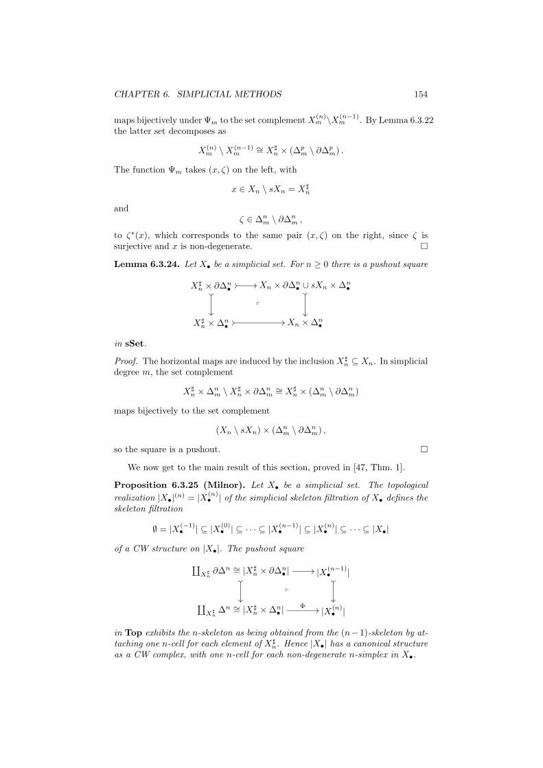
CHAPTER 6. SIMPLICIAL METHODS 154
maps bijectively under Ψm to the set complement X(n)m \X
(n−1)m . By Lemma 6.3.22
the latter set decomposes as
X(n)m \ X(n−1)
m∼= X♯
n × (∆pm \ ∂∆p
m) .
The function Ψm takes (x, ζ) on the left, with
x ∈ Xn \ sXn = X♯n
andζ ∈ ∆n
m \ ∂∆nm ,
to ζ∗(x), which corresponds to the same pair (x, ζ) on the right, since ζ issurjective and x is non-degenerate.
Lemma 6.3.24. Let X• be a simplicial set. For n ≥ 0 there is a pushout square
X♯n × ∂∆n
•// //
²²
²²
p
Xn × ∂∆n• ∪ sXn × ∆n
•²²
²²
X♯n × ∆n
•// // Xn × ∆n
•
in sSet.
Proof. The horizontal maps are induced by the inclusion X♯n ⊆ Xn. In simplicial
degree m, the set complement
X♯n × ∆n
m \ X♯n × ∂∆n
m∼= X♯
n × (∆nm \ ∂∆n
m)
maps bijectively to the set complement
(Xn \ sXn) × (∆nm \ ∂∆n
m) ,
so the square is a pushout.
We now get to the main result of this section, proved in [47, Thm. 1].
Proposition 6.3.25 (Milnor). Let X• be a simplicial set. The topological
realization |X•|(n) = |X
(n)• | of the simplicial skeleton filtration of X• defines the
skeleton filtration
∅ = |X(−1)• | ⊆ |X
(0)• | ⊆ · · · ⊆ |X
(n−1)• | ⊆ |X
(n)• | ⊆ · · · ⊆ |X•|
of a CW structure on |X•|. The pushout square
∐X♯
n∂∆n ∼= |X♯
n × ∂∆n• | //
²²
²²
p
|X(n−1)• |
²²
²²∐X♯
n∆n ∼= |X♯
n × ∆n• |
Φ // |X(n)• |
in Top exhibits the n-skeleton as being obtained from the (n−1)-skeleton by at-taching one n-cell for each element of X♯
n. Hence |X•| has a canonical structureas a CW complex, with one n-cell for each non-degenerate n-simplex in X•.
CHAPTER 6. SIMPLICIAL METHODS 155
Proof. It is clear that |X•| ∼= colimn |X(n)• | has the weak (colimit) topology,
since topological realization commutes with colimits. Combining Lemmas 6.3.23and 6.3.24, we get a pushout square
X♯n × ∂∆n
•//
²²
p
X(n−1)•
²²
X♯n × ∆n
•
Φ• // X(n)•
in sSet, which gives the required pushout square in Top upon topological real-ization.
Lemma 6.3.26. Each simplicial map f• : X• → Y• induces a cellular map|f•| : |X•| → |Y•| upon topological realization. Hence topological realization fac-tors as a (faithful) CW realization functor
| − | : sSet −→ CW
followed by the inclusion CW ⊂ Top.
Proof. The simplicial map f• takes simplices of dimension ≤ n in X• to simplicesof dimension ≤ n in Y•, hence maps the n-skeleton of X• into the n-skeleton ofY•. Thus |f•| maps |X•|
(n) into |Y•|(n), as required.
Definition 6.3.27. A degreewise injective simplicial map f• : X• → Y• is calleda cofibration.
Lemma 6.3.28. If X• ⊆ Y• is a simplicial subset, then |X•| is a subcomplexof |Y•|. More generally, a cofibration f• : X• → Y• (of simplicial sets) inducesan isomorphism of |X•| with its image, as a subcomplex of |Y•|. In particular,|f•| : |X•| → |Y•| is a cofibration (of topological spaces).
Proof. If X• ⊆ Y•, then X♯n ⊆ Y ♯
n for each n ≥ 0, since if x = sj(y) ∈ Xn withy ∈ Yn−1 then sjdj(x) = sjdjsj(y) = sj(y) = x with dj(x) ∈ Xn−1, using thesimplicial identities. Thus x is degenerate in X• if and only if it is degenerate inY•. Hence |X•| is the subcomplex of |Y•| whose n-cells correspond to the subsetX♯
n ⊆ Y ♯n of the n-cells of |Y•|.
A degreewise injective simplicial map f• : X• → Y• factors as an isomor-phism of simplicial sets X•
∼= f•(X•) followed by the simplicial subset inclusionf•(X•) ⊆ Y•, hence induces an isomorphism of CW complexes |X•| ∼= |f•(X•)|followed by the subcomplex inclusion |f•(X•)| ⊆ |Y•|.
Definition 6.3.29. A simplicial set X• is finite if it is generated by finitelymany simplices, or equivalently, if the set of all non-degenerate simplices X♯ =⋃
n≥0 X♯n is finite. This is equivalent to asking that |X•| is a finite CW complex.
Recall Whitehead’s Theorem 5.7.4 on (weak) homotopy equivalences be-tween CW complexes.
Definition 6.3.30. A map f• : X• → Y• of simplicial sets is called a weakhomotopy equivalence if the induced map of CW realizations
|f•| : |X•| −→ |Y•|
is a homotopy equivalence. We then write f• : X•≃−→ Y•.
CHAPTER 6. SIMPLICIAL METHODS 156
Lemma 6.3.31. Let f• : X• → Y• and g• : Y• → Z• be simplicial maps. If twoof the simplicial maps f•, g• and g•f• : X• → Z• are weak homotopy equiva-lences, then so is the third.
Proof. This follows from the two-out-of-three property for homotopy equiva-lences, since |g•f•| = |g•||f•|.
6.4 The role of degenerate simplices
Recall that limits of simplicial sets are constructed degreewise, so that the prod-uct X• × Y• of two simplicial sets has n-simplices Xn × Yn for all n ≥ 0, andsimplicial operators α∗ × α∗ : Xn × Yn → Xm × Ym for all α : [m] → [n] in ∆.
In general, a left adjoint like topological realization will not commute withlimits like products. However, due to the presence of degenerate simplices,topological realization does commute with finite products, as was shown byMilnor [47, Thm. 2]. We shall deduce this from the case when X• and Y• aresimplicial simplices, using the following isomorphism.
Lemma 6.4.1. There is a natural isomorphism
∐
n≥0
Xn × ∆n•/ ∼
∼=−→ X•
where (x, α•(ζ)) ∼ (α∗(x), ζ) for all α : [m] → [n], x ∈ Xn and ζ ∈ ∆m• .
Proof. The simplicial maps Ψ• : Xn×∆n• → X•, taking (x, ζ) to ζ∗(x) for n ≥ 0,
are compatible under ∼, since Ψ•(x, α•(ζ)) = (αζ)∗(x) and Ψ•(α∗(x), ζ) =
ζ∗(α∗(x)). Hence there is an induced map of simplicial sets, as displayed.It suffices to check that this map is a bijection in each simplicial degree p. An
inverse map takes y ∈ Xp to the equivalence class of (y, id[p]) ∈ Xp × ∆pp. One
composite takes y to id∗[p](y) = y. The other composite takes the equivalence
class of (x, ζ), with x ∈ Xn and ζ : [p] → [n], to the class of (ζ∗(x), id[p]). Now(ζ∗(x), id[p]) ∼ (x, ζ•(id[p])) = (x, ζ), so this composite is also the identity.
[[Discuss compatibility of this lemma with Definition 6.2.14.]]
Corollary 6.4.2. There is a coequalizer diagram
∐α : [m]→[n] Xn × ∆m
•
s //
t//
∐n≥0 Xn × ∆n
•// X•
in sSet, where s maps Xn×∆m• → Xm×∆m
• by α∗×id, and t maps Xn×∆m• →
Xn × ∆n• by id × α•.
Proof. The coequalizer in sSet is computed degreewise, and equals the identi-fication space
∐n≥0 Xn × ∆n
•/ ∼ where ∼ identifies s(x, ζ) = (α∗(x), ζ) witht(x, ζ) = (x, α•(ζ)), just as in the previous lemma.
See also Lemma 7.6.4 below.
CHAPTER 6. SIMPLICIAL METHODS 157
Proposition 6.4.3 (Milnor). Let X•, Y• be simplicial sets. The projections
X• X• × Y•pr1oo
pr2 // Y•
in sSet induce a natural homeomorphism
(|pr1|, |pr2|) : |X• × Y•|∼=−→ |X•| × |Y•| ,
where the target is topologized as the product of CW complexes.
Proof. In the special case X• = ∆m• , Y• = ∆n
• , the projections pr1 : ∆m• ×∆n
• →∆m
• , pr2 : ∆m• × ∆n
• → ∆n• induce a homeomorphism
(|pr1|, |pr2|) : |∆m• × ∆n
• |∼=−→ |∆m
• | × |∆n• |
by Proposition 6.1.24, for each m,n ≥ 0. In the general case,
|( ∐
m≥0
Xm × ∆m• / ∼
)×
(∐
n≥0
Yn × ∆n•/ ∼
)|
∼=−→ |X• × Y•|
is a homeomorphism by Lemma 6.4.1 for X• and Y•. By naturality, its compositewith (|pr1|, |pr2|) factors as the chain of homeomorphisms
|( ∐
m≥0
Xm × ∆m• / ∼
)×
(∐
n≥0
Yn × ∆n•/ ∼
)|
∼= |∐
m,n≥0
Xm × Yn × ∆m• × ∆n
•/ ≈ |
∼=∐
m,n≥0
Xm × Yn × |∆m• × ∆n
• |/ ≈
∼=∐
m,n≥0
Xm × Yn × |∆m• | × |∆n
• |/ ≈
∼= |( ∐
m≥0
Xm × ∆m• / ∼
)| × |
(∐
n≥0
Yn × ∆n•/ ∼
)|
∼=−→ |X•| × |Y•|
by Corollary 6.2.22, the special case of simplicial simplices, and Lemma 6.4.1.Hence (|pr1|, |pr2|) is a homeomorphism.
Corollary 6.4.4. CW realization | − | : sSet → CW commutes with finiteproducts.
Proof. This is clear by induction from the previous proposition.
[[Discuss realization and equalizers or finite limits. Failure to commute withinfinite products.]]
Definition 6.4.5. Let f•, g• : X• → Y• be simplicial maps. A simplicial homo-topy from f• to g• is a simplicial map
H• : X• × ∆1• → Y•
such that H• δ1• = f• and H• δ0• = g•. When such an H• exists, we saythat f• and g• are simplicially homotopic, and write H• : f• ≃ g•.
CHAPTER 6. SIMPLICIAL METHODS 158
Remark 6.4.6. Existence of a simplicial homotopy is not in general an equiva-lence relation on simplicial maps X• → Y•. However, simplicial homotopy doesof course generate an equivalence relation on the set of such simplicial maps.[[If Y• is Kan (= fibrant), then simplicial homotopy is an equivalence relationon simplicial maps to Y•.]]
Lemma 6.4.7. A simplicial homotopy H• : f• ≃ g• of simplicial maps X• → Y•
induces a homotopy |H•| : |f•| ≃ |g•| of maps |X•| → |Y•|.
Proof. The homotopy is given by the composite
|X•| × |∆1•|
∼= |X• × ∆1•|
|H•|−→ |Y•| ,
where we identify |∆1| ∼= I = [0, 1] so that the maps |δ1•| and |δ0•| correspondto the end-point inclusions i0 and i1, respectively.
Lemma 6.4.8. A simplicial homotopy H• : f• ≃ g• corresponds to a collectionof functions
hkn : Xn −→ Yn
for n ≥ 0, 0 ≤ k ≤ n + 1, such that
di(hkn(x)) =
hk−1
n−1(di(x)) for 0 ≤ i < k
hkn−1(di(x)) for k ≤ i ≤ n
for n ≥ 1,
sj(hkn(x)) =
hk+1
n+1(sj(x)) for 0 ≤ j < k
hkn+1(sj(x)) for k ≤ j ≤ n
for n ≥ 0, and hn+1n (x) = fn(x), h0
n(x) = gn(x) for all n ≥ 0 and x ∈ Xn.
Proof. The components of H• are functions
Hn : Xn × ∆1n −→ Yn .
We enumerate ∆1n = ζn
0 , . . . , ζnn+1 where ζn
k : [n] → [1] maps 0, . . . , k − 1 to0 and k, . . . , n to 1, see Exercise 6.3.12. Let
hkn(x) = Hn(x, ζn
k )
for x ∈ Xn, 0 ≤ k ≤ n + 1. The naturality conditions
di(Hn(x, ζnk )) = Hn−1(di(x), di(ζ
nk ))
sj(Hn(x, ζnk )) = Hn+1(sj(x), sj(ζ
nk ))
then translate to the displayed relations.
[[Relate to May’s formulation in terms of functions Xn → Yn+1 [42, Def. 5.1].]]Waldhausen [68, p. 335] gives the following reformulation of the data de-
scribing a simplicial homotopy. It is often convenient for defining simplicialhomotopies in a categorical context.
CHAPTER 6. SIMPLICIAL METHODS 159
Definition 6.4.9. Let ∆/[1] be the category of objects in ∆ over [1], withobjects ([n], ζ : [n] → [1]) and morphisms α : [m] → [n] from ([m], ζα) to ([n], ζ).For each simplicial set X•, let X∗ : (∆/[1])op → Set be the composite functor
X∗ : (∆/[1])op −→ ∆op X−→ Set
taking ([n], ζ) to Xn and α to α∗ : Xn → Xm.
Lemma 6.4.10. A simplicial homotopy H• : X•×∆1• → Y•, from f• : X• → Y•
to g : X• → Y•, is equivalent to a natural transformation
h : X∗ =⇒ Y ∗
of functors (∆/[1])op → Set, such that h([n],0) = fn : Xn → Yn and h([n],1) =gn : Xn → Yn for all n ≥ 0, where 0 and 1 denote the constant morphisms to0 ∈ [1] and 1 ∈ [1], respectively.
Proof. A simplicial homotopy H• : X• × ∆1• → Y• consists of functions
Hn : Xn × ∆1n −→ Yn
for n ≥ 0, such that
α∗(Hn(x, ζ)) = Hm(α∗(x), α∗(ζ))
for all α : [m] → [n], x ∈ Xn and ζ : [n] → [1] in ∆1n. Note that α∗(ζ) = ζα.
With these notations, let hζ(x) = Hn(x, ζ). The functions Hn correspond tofunctions
hζ : Xn −→ Yn
for all ζ : [n] → [1], such that
α∗(hζ(x)) = hζα(α∗(x))
for all α : ([m], ζα) → ([n], ζ) and x ∈ Xn.
Xn
hζ//
α∗
²²
Yn
α∗
²²
Xm
hζα// Ym
These correspond precisely to the components h([n],ζ) of a natural transforma-tion h : X∗ ⇒ Y ∗ of functors (∆/[1])op → Set, as claimed.
6.5 Bisimplicial sets
Definition 6.5.1. Let D be any category. A simplicial object X• in D is acontravariant functor
X : ∆op −→ D .
For each n ≥ 0 we write Xn = X([n]) for the object of n-simplices, and foreach morphism α : [m] → [n] in ∆ we write α∗ : Xn → Xm for the simplicial
CHAPTER 6. SIMPLICIAL METHODS 160
structure morphism in D . It suffices to specify the face and degeneracy mor-phisms di : Xn → Xn−1 and sj : Xn → Xn+1, subject to the simplicial identitiesof Lemma 6.2.7. We may write
[n] 7−→ Xn
for such a functor.A map f• : X• → Y• of simplicial objects in D is a natural transformation
f : X =⇒ Y .
It is determined by its components fn : Xn → Yn for n ≥ 0, which are morphismsin D such that α∗fn = fmα∗ for α : [m] → [n]. It suffices to check that difn =fn−1di and sjfn = fn+1sj for all i and j. We may write
[n] 7−→ (fn : Xn → Yn)
for such a natural transformation.We write
sD = Fun(∆op,D)
for the category of simplicial objects in D .
Example 6.5.2. Quoting [67, p. 163], if the objects of D are called things, thenthe simplicial objects in D are called simplicial things.
(a) A simplicial set is a simplicial object in Set.
(b) A based simplicial set is the same as a simplicial based set, i.e., a simplicialobject in Set∗.
(c) A simplicial space Y• is a simplicial object in Top, with a space Yn ofn-simplices for each n ≥ 0, and a map α∗ : Yn → Ym for each α : [m] → [n]in ∆.
(d) A simplicial category C• is a simplicial object in Cat, with a categoryCn of n-simplices for each n ≥ 0, and a functor α∗ : Cn → Cm for eachmorphism α in ∆.
Example 6.5.3. An object X of a category D can be viewed as a constantsimplicial object in sD , given by the constant functor X : ∆op → D taking eachobject [n] to X and each morphism α to idX . [[No change in the notation?]]Given a simplicial object Y• in D , we may view its degree zero part Y0 as aconstant simplicial object. There is then a unique simplicial map
ρ∗ : Y0 −→ Y•
that is the identity in degree 0, called the inclusion of the zero-simplices. Itis given in simplicial degree n by the simplicial operator ρ∗n : Y0 → Yn, whereρ : [n] → [0] is the unique morphism in ∆. For each morphism α : [m] → [n] in∆ the simplicial operators α∗ = id : Y0 → Y0 and α∗ : Yn → Ym commute withρ∗, in the sense that α∗ ρ∗n = ρ∗m id, since ρn α = ρm : [m] → [0]. Henceρ∗ is a simplicial map. The “constant simplicial object” functor D → sD isleft adjoint to the “degree zero part” functor sD → D , with ρ∗ as adjunctioncounit.
CHAPTER 6. SIMPLICIAL METHODS 161
Definition 6.5.4. A bisimplicial set X•,• is a contravariant functor
X : ∆op × ∆op −→ Set .
We write Xm,n = X([m], [n]) for the set of (m,n)-bisimplices, and may displayX as
[m], [n] 7−→ Xm,n .
A map f•,• : X•,• → Y•,• is a natural transformation f : X ⇒ Y . Its compo-nents are functions fm,n : Xm,n → Ym,n for all m,n ≥ 0, commuting with thebisimplicial structure maps (α, β)∗ for all α : [p] → [m] and β : [q] → [n].
Lemma 6.5.5. The category ssSet of bisimplicial sets is identified with thecategory ssSet of simplicial objects in simplicial sets, via the isomorphism
ssSet = Fun(∆op × ∆op,Set) ∼= Fun(∆op,Fun(∆op,Set)) = ssSet .
A bisimplicial set X•,• then corresponds to the simplicial simplicial set
[m] 7−→ Xm,• ,
with m-simplices the simplicial set Xm,• : [n] 7−→ Xm,n having simplicial struc-ture maps the functions β∗ = (id[m], β)∗. The simplicial structure maps of[m] 7→ Xm,• are simplicial maps α∗
• with n-th component α∗n = (α, id[n])
∗.
Proof. See Lemma 3.1.13.
Remark 6.5.6. In a bisimplicial set X•,• we may refer to the first and sec-ond simplicial directions as the left hand and right hand simplicial directions,respectively. Under the identification of Lemma 6.5.5, we can think of these asexternal and internal simplicial directions, respectively.
Remark 6.5.7. The algebraic K-theory of a Waldhausen category will be de-fined as the (total) topological realization of a bisimplicial set associated to asimplicial category. We shall therefore need to be able to manipulate bisimplicialsets and certain associated simplicial spaces.
Definition 6.5.8. The degreewise topological realization of a bisimplicial setX•,• is the simplicial space
[m] 7−→ |Xm,•| =∐
n≥0
Xm,n × ∆n/∼r
given by the composite functor
∆op X−→ sSet
|−|−→ Top .
Here ∼r refers to the identifications (x, β∗(η)) ∼ (β∗(x), η) involving the righthand (= internal) simplicial structure of X•,•, for β : [q] → [n], x ∈ Xm,n andη ∈ ∆q.
Definition 6.5.9. The topological realization of a simplicial space Z• is theidentification space
|Z•| =∐
m≥0
Zm × ∆m/ ∼
where Zm×∆m is given the product topology,∐
m≥0 Zm×∆m is the coproduct,and ∼ is generated by (z, α∗(ξ)) ∼ (α∗(z), ξ) for α : [p] → [m], z ∈ Zm andξ ∈ ∆p.
CHAPTER 6. SIMPLICIAL METHODS 162
For general simplicial spaces, this can be a badly behaved identificationspace. However, for simplicial spaces arising by degreewise topological realiza-tion of bisimplicial sets, there is no difficulty.
Definition 6.5.10. The total topological realization of a bisimplicial set X•,•
is the identification space
‖X•,•‖ =∐
m,n≥0
Xm,n × ∆m × ∆n/ ≈
where Xm,n×∆m×∆n is homeomorphic to the disjoint union of one copy of theproduct ∆m × ∆n for each element in Xm,n, and ≈ is the equivalence relationgenerated by
(x, (α, β)∗(ξ, η)) ≈ ((α, β)∗(x), (ξ, η))
for α : [p] → [m], β : [q] → [n], x ∈ Xm,n, ξ ∈ ∆p, η ∈ ∆q.
Lemma 6.5.11. There is a natural homeomorphism
‖X•,•‖ ∼= | [m] 7→ |Xm,•| | .
Proof. All terms in
| [m] 7→ |Xm,•| | =∐
m≥0
|Xm,•| × ∆m/ ∼
=∐
m≥0
(∐
n≥0
Xm,n × ∆n/ ∼r
)× ∆m/ ∼
∼=∐
m,n≥0
Xm,n × ∆m × ∆n/ ≈
= ‖X•,•‖
are obtained from∐
m,n≥0 Xm,n ×∆m ×∆n by the same identifications. [[Someexplanation of the interaction of products and identification spaces might beappropriate. Alternatively, consider realization to CW instead of Top.]]
Definition 6.5.12. A map f•,• : X•,• → Y•,• of bisimplicial sets is a weakhomotopy equivalence if the total topological realization
‖f•,•‖ : ‖X•,•‖ → ‖Y•,•‖
is a homotopy equivalence.
Definition 6.5.13. The simplicial realization of a bisimplicial set X•,• is thesimplicial set ∐
m≥0
Xm,• × ∆m• / ∼l
where Xm,• × ∆m• is the product simplicial set, with n-simplices Xm,n × ∆m
n ,∐m≥0 Xm,• × ∆m
• is the coproduct of simplicial sets, and ∼l is the equivalencerelation generated in each simplicial degree n by the relations (x, α•(ζ)) ∼l
(α∗•(x), ζ) for α : [p] → [m], x ∈ Xm,n and ζ ∈ ∆p
n, coming from the left hand(= external) simplicial structure on X•,•.
CHAPTER 6. SIMPLICIAL METHODS 163
Lemma 6.5.14. The topological realization of the simplicial realization of abisimplicial set is naturally homeomorphic with the total topological realization.
Proof.
|∐
m≥0
Xm,• × ∆m• / ∼l | ∼=
∐
m≥0
|Xm,• × ∆m• |/ ∼
∼=∐
m≥0
|Xm,•| × |∆m• |/ ∼
∼=∐
m≥0
|Xm,•| × ∆m/ ∼
∼= ‖X•,•‖
by Corollary 6.2.22, Proposition 6.4.3, Lemma 6.3.8 and Lemma 6.5.11.
Definition 6.5.15. The diagonal of a bisimplicial set X•,• is the simplicial setdiag(X)•, with n-simplices
diag(X)n = Xn,n
for all n ≥ 0, and simplicial structure maps α∗ = (α, α)∗ : diag(X)n → diag(X)m
for all α : [m] → [n] in ∆. It equals the composite functor
∆op ∆−→ ∆op × ∆op X
−→ Set ,
where ∆ denotes the diagonal functor. Any map f•,• : X•,• → Y•,• of bisimpli-cial sets induces a map diag(f)• : diag(X)• → diag(Y )• of diagonal simplicialsets, and
diag : ssSet → sSet
is a functor.
Proposition 6.5.16. The diagonal of a bisimplicial set is naturally isomorphicto the simplicial realization:
diag(X)• ∼=∐
m≥0
Xm,• × ∆m• / ∼l
Hence there is a natural homeomorphism
|diag(X)•| ∼= ‖X•,•‖ .
Proof. For each m ≥ 0 there is a simplicial map
Ψ• : Xm,• × ∆m• −→ diag(X)•
given in simplicial degree n by
(x, ζ) 7→ ζ∗n(x) = (ζ, id[n])∗(x) ,
for x ∈ Xm,n, ζ ∈ ∆mn . This is a simplicial map, since for β : [q] → [n],
β∗(x, ζ) = (β∗(x), β∗(ζ)) = ((id[m], β)∗(x), ζβ)
CHAPTER 6. SIMPLICIAL METHODS 164
maps to
(ζβ, id[n])∗((id[m], β)∗(x)) = (β, β)∗(ζ, id[n])
∗(x) = (β, β)∗(ζ∗n(x)) .
The maps Ψ• are compatible under the relation ∼l, since for α : [p] → [m],x ∈ Xm,n and ζ ∈ ∆n
p the class (x, α•(ζ)) = (x, αζ) maps to (αζ)∗n(x), whilethe class (α∗
n(x), ζ) maps to ζ∗n(α∗n(x)), and these values are equal. Hence there
is a well-defined simplicial map
∐
m≥0
Xm,• × ∆m• / ∼l −→ diag(X)• .
There is also a simplicial map the other way, taking x ∈ diag(X)n = Xn,n tothe equivalence class of the n-simplex (x, id[n]) in Xn,• × ∆n
• . This is sim-plicial, since for β : [q] → [n] the q-simplex (β, β)∗(x) in diag(X)q = Xq,q
maps to ((β, β)∗(x), id[q]), while β∗(x, id[n]) = ((id[n], β)∗(x), β) is equivalentto β∗
q ((id[n], β)∗(x), id[q]) = ((β, β)∗(x), id[q]).The composite self-map of diag(X)• takes x ∈ Xn,n to id∗[n](x) = x, hence
equals the identity.The other composite takes the class of (x, ζ) to the class of (ζ∗n(x), id[n]),
which under ∼l is identified with (x, ζn), so also this composite is the identity.The natural homeomorphism is now obtained by passing to topological re-
alization, and using Lemma 6.5.14.
Remark 6.5.17. This proposition may seem surprising, since it exhibits ahomeomorphism between the different-looking identification spaces
∐
p≥0
Xp,p × ∆p/ ∼
and ∐
m,n≥0
Xm,n × ∆m × ∆n/ ≈ .
It provides a key simplifying tool in the theory of bisimplicial sets, since for thepurposes of homotopy theory, the topological realization of X•,• is the same asthat of the diagonal simplicial set diag(X)•. The additional simplicial directiondoes therefore not contribute essentially to the form of the topological realiza-tion. More generally, for multi-simplicial sets given by contravariant functors
X : ∆op × · · · × ∆op → Set ,
the total topological realization is naturally homeomorphic to the topologicalrealization of the diagonal simplicial set X ∆, where
∆: ∆op → ∆op × · · · × ∆op
is the diagonal functor.
Corollary 6.5.18. A map f•,• : X•,• → Y•,• of bisimplicial sets is a weakhomotopy equivalence if and only if the diagonal map diag(f)• : diag(X)• →diag(Y )• of simplicial sets is a weak homotopy equivalence.
CHAPTER 6. SIMPLICIAL METHODS 165
Proof. This is clear from the commutative square
|diag(X)•|| diag(f)•|
//
∼=
²²
|diag(Y )•|
∼=
²²
‖X•,•‖|f•,•|
// ‖Y•,•‖
expressing naturality in Proposition 6.5.16.
[[External product of simplicial sets, (X• ⊠ Y•) : [m], [n] 7→ Xm × Yn.]][[Isomorphism of bisimplicial sets X•,•
∼=∐
m,n≥0 Xm,n × ∆m• ⊠ ∆n
•/ ≈.]][[May interchange left and right, and consider [n] 7→ X•,n, etc.]]
6.6 The realization lemma
The following useful result is stated in [67, Lem. 5.1].
Proposition 6.6.1 (Realization lemma). Let f•,• : X•,• −→ Y•,• be a mapof bisimplicial sets, such that for each m ≥ 0 the map
fm,• : Xm,• −→ Ym,•
of simplicial sets is a weak homotopy equivalence. Then f•,• is a weak homotopyequivalence.
The naming of this result is perhaps clearer from the following restatement.
Corollary 6.6.2. Let f•,• : X•,• −→ Y•,• be a map of bisimplicial sets, and letZm = |Xm,•|, Wm = |Ym,•| and gm = |fm,•|, so that g• : Z• → W• is a map ofsimplicial spaces. If
gm : Zm≃−→ Wm
is a homotopy equivalence for each m ≥ 0, then the induced map of topologicalrealizations
|g•| : |Z•|≃−→ |W•|
is a homotopy equivalence.
Proof. This is clear by the realization lemma and Lemma 6.5.11.
[[More general statement, cite Segal [60].]]
Remark 6.6.3. The roles of the left and right simplicial directions may ofcourse be interchanged: If f•,n is a weak homotopy equivalence for each n ≥ 0,then f•,• is a homotopy equivalence.
As a first step towards proving the realization lemma, we analyze the sim-plicial subsets of degenerate simplices. We follow the notation of [22, ??].
Definition 6.6.4. Let k ≥ 0. For each 0 ≤ j < k let sj(Xk−1,•) ⊆ Xk,• bethe simplicial subset given by the image of sj,• = (σj , id)∗ : Xk−1,• → Xk,•. Foreach −1 ≤ ℓ < k let
s[ℓ]Xk,• =⋃
0≤j≤ℓ
sj(Xk−1,•) ,
CHAPTER 6. SIMPLICIAL METHODS 166
and letsXk,• = s[k−1]Xk,• =
⋃
0≤j<k
sj(Xk−1,•)
be the simplicial subset of degenerate k-simplices.
Lemma 6.6.5. For each 0 ≤ ℓ < k there is a pushout square
s[ℓ−1]Xk−1,• //
²²
²²
p
s[ℓ−1]Xk,•²²
²²
Xk−1,•sℓ,•
// s[ℓ]Xk,•
in sSet.
Proof. Since s[ℓ]Xk,• is defined as the union of s[ℓ−1]Xk,• and the image of sℓ
on Xk−1,•, it suffices to show that s[ℓ−1]Xk−1,• is the preimage of s[ℓ−1]Xk,•
under sℓ. Suppose that y ∈ Xk−1,• satisfies sℓ(y) = sj(z) for some 0 ≤ j < ℓand z ∈ Xk−1,•. Then by the simplicial identities,
y = dℓ+1(sℓ(y)) = dℓ+1(sj(z)) = sj(dℓ(z)) ,
so y ∈ s[ℓ−1]Xk−1,•. Conversely, suppose that y = sj(w) for some 0 ≤ j < ℓ andw ∈ Xk−2,•. Then, by another case of the simplicial identities,
sℓ(y) = sℓ(sj(w)) = sj(sℓ−1(w))
and sℓ(y) ∈ s[ℓ−1]Xk,•.
Corollary 6.6.6. Let f•,• : X•,• −→ Y•,• be such that
fm,• : Xm,• −→ Ym,•
is a weak homotopy equivalence for each m ≥ 0. Then the restricted map
sfk,• : sXk,• −→ sYk,•
is a weak homotopy equivalence for each k ≥ 0.
Proof. We prove by induction on k ≥ 0 and −1 ≤ ℓ < k that s[ℓ]fk,• : s[ℓ]Xk,• →s[ℓ]Yk,• is a weak homotopy equivalence. This is clear for ℓ = −1. For 0 ≤ ℓ < kit follows by the gluing lemma, Lemma 6.6.5, and the inductive hypothesis.
Definition 6.6.7. For each k ≥ −1, let the external k-skeleton
X(k)•,• ⊆ X•,•
be the bisimplicial subset generated by the (m, q)-bisimplices with m ≤ k. It isthe image of the canonical map
∐
m≤k
Xm,• × ∆m• −→ X•,• .
Then X(k)•,q is the simplicial k-skeleton of X•,q for each q ≥ 0. Let diag(X(k))• ⊆
diag(X)• be the diagonal simplicial set, with q-simplices diag(X(k))q = X(k)q,q ⊆
Xq,q.
CHAPTER 6. SIMPLICIAL METHODS 167
Proof of the realization lemma. We shall prove by induction that the restrictedmap
diag(f (k))• : diag(X(k))• −→ diag(Y (k))•
is a weak homotopy equivalence, for each k ≥ −1. This is clear for k = −1,since all (−1)-skeleta are empty. Applying topological realization, and usingLemma 5.5.7 to pass to the colimit as k → ∞, it then follows that
|diag(f)•| : |diag(X)•| −→ |diag(Y )•|
is a homotopy equivalence, which by Corollary 6.5.18 is what we need to prove.By Lemma 6.3.23 applied to the simplicial set X•,q there is a pushout square
Xk,q × ∂∆k• ∪ sXk,q × ∆k
•//
²²
²²
p
X(k−1)•,q
²²
²²
Xk,q × ∆k•
// X(k)•,q
in sSet for each q ≥ 0, hence also a pushout square
Xk,• × ∂∆k• ∪ sXk,• × ∆k
•//
²²
²²
p
diag(X(k−1))•²²
²²
Xk,• × ∆k•
// diag(X(k))•
(6.2)
in sSet. The vertical maps are inclusions, hence cofibrations.By assumption, each map Xm,• → Ym,• is a weak homotopy equivalence,
so by Corollary 6.6.6, each restricted map sXk,• → sYk,• is a weak homotopyequivalence. It follows, from the commutation of products with topologicalrealization, that the four maps
Xk,• × ∆k• −→ Yk,• × ∆k
•
Xk,• × ∂∆k• −→ Yk,• × ∂∆k
•
sXk,• × ∆k• −→ sYk,• × ∆k
•
sXk,• × ∂∆k• −→ sYk,• × ∂∆k
•
are weak homotopy equivalences. By the gluing lemma applied to the pushoutsquare
sXk,• × ∂∆k•
// //
²²
²²
p
sXk,• × ∆k•
²²
²²
Xk,• × ∂∆k•
// // Xk,• × ∂∆k• ∪ sXk,• × ∆k
•
the union map
Xk,• × ∂∆k• ∪ sXk,• × ∆k
• −→ Yk,• × ∂∆k• ∪ sYk,• × ∆k
•
is a weak homotopy equivalence.By another application of the gluing lemma, using the pushout square (6.2)
and the inductive hypothesis that diag(f (k−1))• is a weak homotopy equivalence,it follows that diag(f (k))• is a weak homotopy equivalence. This completes theinductive proof.
CHAPTER 6. SIMPLICIAL METHODS 168
Example 6.6.8. Let Y•,• be a bisimplicial set, such that each degeneracy map
ρ∗m : Y0,• −→ Ym,•
is a weak homotopy equivalence. Then the inclusion of zero-simplices (see Ex-ample 6.5.3)
ρ∗ : Y0,• −→ Y•,•
is a weak homotopy equivalence, by the realization lemma.
6.7 Subdivision
[[Segal’s edgewise subdivision.]][[The Bokstedt–Hsiang–Madsen edgewise subdivision.]][[Barycentric subdivision and Kan normal subdivision.]]
6.8 Realization of fibrations
The following is a special case of the Bousfield–Friedlander fibration theorem[8, B.4]. We outline Waldhausen’s argument [67, 5.2], which in turn extends aone-line proof of a special case due to Dieter Puppe.
Definition 6.8.1. A diagram V → X → Y of topological spaces is a fibrationup to homotopy if the composite map V → Y is constant [[to a point z0 ∈ Y ]],and if the induced map from V to the homotopy fiber of X → Y [[at z0]] is ahomotopy equivalence.
A diagram of simplicial sets V• → X• → Y• is a fibration up to homotopyif the diagram |V•| → |X•| → |Y•| obtained by topological realization has thisproperty, and similarly for multi-simplicial sets, categories, etc.
Proposition 6.8.2. Let V•,• → X•,• → Y•,• be a diagram of bisimplicial setssuch that V•,• → Y•,• is constant. Suppose that
Vm,• −→ Xm,• −→ Ym,•
is a fibration up to homotopy, for each m ≥ 0. Suppose furthermore that Ym,•
is connected, for each m ≥ 0. Then
V•,• −→ X•,• −→ Y•,•
is a fibration up to homotopy.
Proof. Consider first the special case when there is a bisimplicial group G•,•
that acts from the right on a bisimplicial set W•,•, and the diagram has theform
Wm,• −→ Wm,• ×Gm,•E•Gm,• −→ B•Gm,• ,
(balanced product over Gm,•) compatibly for each m ≥ 0. [[Reference for barconstructions. Implicitly pass to diagonal in B•Gm,•.]] The topological realiza-tion can then be written as
W −→ W ×G EG −→ BG
CHAPTER 6. SIMPLICIAL METHODS 169
where G = ‖G•,•‖ is a (cofibrantly based) topological group acting on the righton the space W = ‖W•,•‖. This is the fiber bundle associated to the principalG-bundle G → EG → BG, see [63] and also [41, 1.5]. In particular it is ahomotopy fiber sequence, since the base is numerable [[Reference]].
To handle the general case, we will the Kan loop group functor, which toeach connected pointed simplicial set Z• associates a (degreewise free) simplicialgroup G(Z•), such that |G(Z•)| ≃ Ω|Z•|. More precisely, there is a principalG(Z•)-bundle
ΓZ• −→ ΓZ•
with ΓZ• weakly contractible, and a pointed weak equivalence Z•≃−→ ΓZ•,
all of which depend functorially on Z•. See Kan’s original article [32] andWaldhausen’s remake [69]. [[Discuss preferred base points in ΓZ• and ΓZ•.]]
For each m ≥ 0, form the Kan loop group Gm,• = G(Ym,•) and the principal
Gm,•-bundle ΓYm,• → ΓYm,•. Let
Wm,• = Xm,• ×ΓYm,•ΓYm,•
denote the pullback along the composite map Xm,• → Ym,• → ΓYm,•. Here thesubscript indicates the pullback with respect to the maps to ΓYm,•. We get acommutative diagram
Vm,• //
=
²²
Xm,• //
=
²²
Ym,•
≃
²²
Vm,• // Xm,• // ΓYm,•
Vm,• //
=
OO
Wm,•f
//
OO
q
ΓYm,•
OO
The middle row is a fibration up to homotopy since Ym,•≃−→ ΓYm,• is a weak
homotopy equivalence, so that the homotopy fibers of |Xm,•| → |Ym,•| and|Xm,•| → |ΓYm,•| are homotopy equivalent.
The free right Gm,•-action on ΓYm,• pulls back to a free action on Wm,•, and
the map labeled f is equivariant. Applying the Borel construction (−) ×Gm,•
E•Gm,• (where the subscript now denotes the balanced product with respect tothe Gm,•-actions), we get the upper part of the following commutative diagram.
Vm,• // Xm,• // ΓYm,•
Vm,• //
=
OO
≃
²²
Wm,• ×Gm,•E•Gm,• //
≃
OO
=
²²
q
ΓYm,• ×Gm,•E•Gm,•
≃
OO
≃
²²
Wm,• // Wm,• ×Gm,•E•Gm,• // B•Gm,•
The right hand vertical map is induced by the collapse map ΓYm,• → ∗, andthe lower row is the fiber bundle associated to the Gm,•-action on Wm,•.
CHAPTER 6. SIMPLICIAL METHODS 170
The maps in the middle and right hand columns are weak equivalences,since Wm,• → Xm,•, ΓYm,• → ΓYm,• and E•Gm,• → B•Gm,• are principal
Gm,•-bundles, and E•Gm,• and ΓYm,• are contractible.It follows that the middle row is a fibration up to homotopy. By comparing
the long exact sequences in homotopy for the middle and lower rows, and usingthe five-lemma, it follows that the left hand vertical map Vm,• → Wm,• is aweak homotopy equivalence.
By functoriality of the Kan loop group construction, we now have a diagramof bisimplicial sets
V•,• //
=
²²
X•,• //
=
²²
Y•,•
≃
²²
V•,• // X•,• // ΓY•,•
V•,• //
=
OO
≃
²²
W•,• ×G•,•E•G•,• //
≃
OO
=
²²
ΓY•,• ×G•,•E•G•,•
≃
OO
≃
²²
W•,• // W•,• ×G•,•E•G•,• // B•G•,•
where all vertical maps are weak equivalences, by the the discussion above foreach m ≥ 0 and the realization lemma, and all horizontal composites are con-stant. By the first special case, the lower row is a fibration up to homotopy. Itfollows that also the upper row is a fibration up to homotopy, as desired.
Chapter 7
Homotopy theory of
categories
We now turn to the first chapter of Quillen’s paper [55], on the classifying spaceof a small category.
7.1 Nerves and classifying spaces
Recall from Definition 2.9.4 that we view the totally ordered set
[n] = 0 < 1 < · · · < n
as a small category.
Definition 7.1.1. The nerve of a small category C is the simplicial set N•C
with n-simplicesNnC = Cat([n],C )
for n ≥ 0, and structure maps
α∗ = Cat(α,C ) : NnC = Cat([n],C ) −→ Cat([m],C ) = NmC
for each morphism α : [m] → [n] in ∆. Here α∗ takes an n-simplex x : [n] → C
to the compositeα∗(x) = x α : [m] −→ C .
In other words, NnC is the set of all diagrams
X0f1−→ X1
f2−→ . . .
fn−→ Xn
of n composable morphisms in C . The i-th face operator di : NnC → Nn−1C ,for 0 ≤ i ≤ n ≥ 1, takes the n-simplex above to the (n − 1)-simplex
X1f2−→ . . .
fn−→ Xn
for i = 0,
X0f1−→ . . .
fi−1−→ Xi−1
fi+1fi−→ Xi+1
fi+2−→ . . .
fn−→ Xn
171
CHAPTER 7. HOMOTOPY THEORY OF CATEGORIES 172
for 0 < i < n, and
X0f1−→ . . .
fn−1−→ Xn−1
for i = n. The j-th degeneracy operator sj : Xn → Xn+1, for 0 ≤ j ≤ n, takesthe n-simplex above to the (n + 1)-simplex
X0f1−→ . . .
fj−→ Xj
idXj−→ Xj
fj+1−→ . . .
fn−→ Xn .
Definition 7.1.2. Let F : C → D be a functor between small categories. Theinduced map of nerves
N•F : N•C −→ N•D
is the map of simplicial sets given in degree n by the function
NnF = Cat([n], F ) : NnC = Cat([n],C ) −→ Cat([n],D) = NnD .
Here NnF takes an n-simplex x : [n] → C to the composite
(NnF )(x) = F x : [n] −→ D .
In other words, this is the function taking the diagram
X0f1−→ X1
f2−→ . . .
fn−→ Xn
of n composable morphisms in C to the diagram
F (X0)F (f1)−→ F (X1)
F (f2)−→ . . .
F (fn)−→ F (Xn)
of n composable morphisms in D .
Example 7.1.3. N•[n] = ∆n• for all n ≥ 0, and N•α = α• for all α in ∆. In
particular, N•[1] = ∆1•, where [1] is the category 0 < 1.
Definition 7.1.4. We will use the bar notation [fn| . . . |f1]X0 for the n-simplex
X0f1−→ . . .
fn−→ Xn
in N•C . Then
di([fn| . . . |f1]X0) =
[fn| . . . |f2]X1 for i = 0,
[fn| . . . |fi+1fi| . . . |f1]X0 for 0 < i < n,
[fn−1| . . . |f1]X0 for i = n,
andsj([fn| . . . |f1]X0) = [fn| . . . |idXj
| . . . |f1]X0
for 0 ≤ j ≤ n, while
(NnF )([fn| . . . |f1]X0) = [F (fn)| . . . |F (f1)]F (X0)
for n ≥ 0.
CHAPTER 7. HOMOTOPY THEORY OF CATEGORIES 173
Definition 7.1.5. For 0 ≤ i ≤ n, let the i-th vertex morphism ǫi : [0] → [n] in∆ be given by ǫi(0) = i. For 1 ≤ i ≤ n let the i-th edge morphism ηi : [1] → [n]in ∆ be given by ηi(0) = i − 1 and ηi(1) = i. In the nerve N•C of a categorywe can recover the objects and morphisms in a diagram
X0f1−→ . . .
fn−→ Xn
corresponding to an n-simplex σ = [fn| . . . |f1]X0 by the formulas Xi = ǫ∗i (σ)for 0 ≤ i ≤ n and fi = η∗
i (σ) for 1 ≤ i ≤ n.
Lemma 7.1.6. The rules C 7→ N•C and F 7→ N•F define a full and faithfulfunctor
N• : Cat −→ sSet .
Proof. Functoriality is clear. Given small categories C and D , we must provethat
N• : Cat(C ,D) −→ sSet(N•C , N•D)
is bijective.Suppose given a simplicial map h• : N•C → N•D . For each X in obj(C ) =
N0C , let H(X) = h0(X) in obj(D) = N0D . For each f : X → Y in C (X,Y ),view f = [f ]X as an element in N1C with d0(f) = Y and d1(f) = X, and letH(f) = h1(f) ∈ N1D . Then d0(H(f)) = d0(h1(f)) = h0(d0(f)) = h0(Y ) =H(Y ) and d1(H(f)) = d1(h1(f)) = h0(d1(f)) = h0(X) = H(X), since h• is asimplicial map, so H(f) : H(X) → H(Y ) lies in D(H(X),H(Y )).
We check that the rules X 7→ H(X) and f 7→ H(f) define a functor. Iff = idX ∈ N1C then f = s0(X) for X ∈ N0C , so H(f) = h1(s0(X)) =s0(h0(X)) = s0(H(X)) = idH(X). If g : Y → Z in C then we view
Xf
−→ Yg
−→ Z
as a 2-simplex σ = [g|f ]X ∈ N2C , with d0(σ) = g, d1(σ) = gf and d2(σ) = f inN1C . Applying the simplicial map h• we get a 2-simplex τ = h2([g|f ]X) ∈ N2D
with d0(τ)) = h1(g) = H(g), d1(τ)) = h1(gf) = H(gf) and d2(τ)) = h1(f) =H(f). Hence τ is the 2-simplex
H(X)H(f)−→ H(Y )
H(g)−→ H(Z)
in N•D , denoted [H(g)|H(f)]H(X), with the property that H(g) H(f) =d1(τ) = H(gf).
Starting with a functor F : C → D and applying this construction to h• =N•F , it is clear that the resulting functor H agrees with F on objects andmorphisms, so that F = H.
Conversely, starting with a simplicial map h• : N•C → N•D , we claim thath• equals the nerve map N•H of the associated functor H. To see this, consideran n-simplex
X0f1−→ . . .
fn−→ Xn
in N•C , say σ = [fn| . . . |f1]X0. It is mapped under N•H to the n-simplex
H(X0)H(f1)−→ . . .
H(fn)−→ H(Xn)
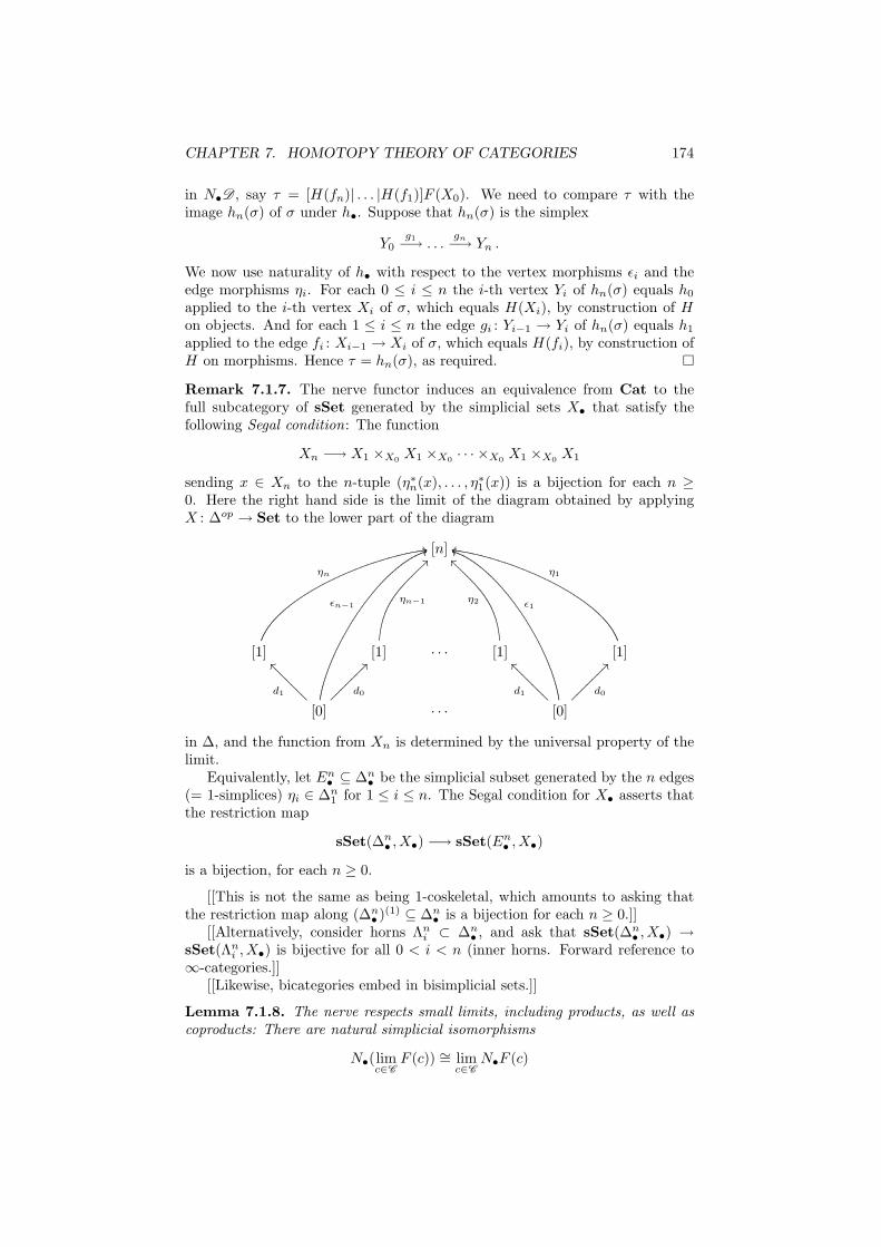
CHAPTER 7. HOMOTOPY THEORY OF CATEGORIES 174
in N•D , say τ = [H(fn)| . . . |H(f1)]F (X0). We need to compare τ with theimage hn(σ) of σ under h•. Suppose that hn(σ) is the simplex
Y0g1−→ . . .
gn−→ Yn .
We now use naturality of h• with respect to the vertex morphisms ǫi and theedge morphisms ηi. For each 0 ≤ i ≤ n the i-th vertex Yi of hn(σ) equals h0
applied to the i-th vertex Xi of σ, which equals H(Xi), by construction of Hon objects. And for each 1 ≤ i ≤ n the edge gi : Yi−1 → Yi of hn(σ) equals h1
applied to the edge fi : Xi−1 → Xi of σ, which equals H(fi), by construction ofH on morphisms. Hence τ = hn(σ), as required.
Remark 7.1.7. The nerve functor induces an equivalence from Cat to thefull subcategory of sSet generated by the simplicial sets X• that satisfy thefollowing Segal condition: The function
Xn −→ X1 ×X0X1 ×X0
· · · ×X0X1 ×X0
X1
sending x ∈ Xn to the n-tuple (η∗n(x), . . . , η∗
1(x)) is a bijection for each n ≥0. Here the right hand side is the limit of the diagram obtained by applyingX : ∆op → Set to the lower part of the diagram
[n]
[1]
ηn
11
[1]
ηn−1
>>
. . . [1]
η2
``
[1]
η1
mm
[0]
d1
__??????? d0
??ÄÄÄÄÄÄÄ
ǫn−1
44
. . . [0]
d1
__??????? d0
??ÄÄÄÄÄÄÄ
ǫ1
jj
in ∆, and the function from Xn is determined by the universal property of thelimit.
Equivalently, let En• ⊆ ∆n
• be the simplicial subset generated by the n edges(= 1-simplices) ηi ∈ ∆n
1 for 1 ≤ i ≤ n. The Segal condition for X• asserts thatthe restriction map
sSet(∆n• ,X•) −→ sSet(En
• ,X•)
is a bijection, for each n ≥ 0.
[[This is not the same as being 1-coskeletal, which amounts to asking thatthe restriction map along (∆n
• )(1) ⊆ ∆n• is a bijection for each n ≥ 0.]]
[[Alternatively, consider horns Λni ⊂ ∆n
• , and ask that sSet(∆n• ,X•) →
sSet(Λni ,X•) is bijective for all 0 < i < n (inner horns. Forward reference to
∞-categories.]][[Likewise, bicategories embed in bisimplicial sets.]]
Lemma 7.1.8. The nerve respects small limits, including products, as well ascoproducts: There are natural simplicial isomorphisms
N•(limc∈C
F (c)) ∼= limc∈C
N•F (c)
CHAPTER 7. HOMOTOPY THEORY OF CATEGORIES 175
for each diagram F : C → Cat, and
N•(∏
i∈I
Ci) ∼=∏
i∈I
N•Ci
N•(∐
i∈I
Ci) ∼=∐
i∈I
N•Ci
for each family (Ci)i∈I of small categories.
Proof. Functors [n] → limc∈C F (c) correspond to families of functors [n] → F (c)for c in C , compatible under the morphisms of C . Each functor [n] →
∐i∈I Ci
factors through a unique Ci.
Remark 7.1.9. The nerve N• admits a left adjoint, L : sSet → Cat, takinga simplicial set X• to a coequalizer
∐α : [m]→[n] Xn × [m]
s //
t//
∐n≥0 Xn × [n] // L (X•)
in Cat. Here Xn × [n] denotes∐
Xn[n], and so on. Functors F : L (X•) → D
correspond to compatible families of functors Fn : Xn × [n] → D for n ≥ 0, orequivalently, to compatible functions Gn : Xn → NnD . These are the same assimplicial maps G• : X• → N•D .
Remark 7.1.10. The nerve does not preserve general colimits. For example,for suitable functors s and t, the coequalizer of the nerve of the diagram
[1] ⊔ [1]s //
t// [2] ⊔ [2]
is not the nerve of a category. [[Elaborate?]]
Lemma 7.1.11. The nerve of the opposite category is the opposite simplicialset of the nerve:
N•(Cop) = N•(C )op
[[Proof]]
Definition 7.1.12. The classifying space of a small category C is the topolog-ical realization
|C | = |N•C |
of its nerve. It is a CW complex with one n-cell for each non-degenerate n-simplex in N•C , i.e., for each chain
X0f1−→ . . .
fn−→ Xn
of n composable, non-identity morphisms in C .Each functor F : C → D of small categories induces a cellular map
|F | = |N•F | : |C | −→ |D |
of classifying spaces. The classifying space defines a functor
| − | : Cat −→ CW ⊂ Top .
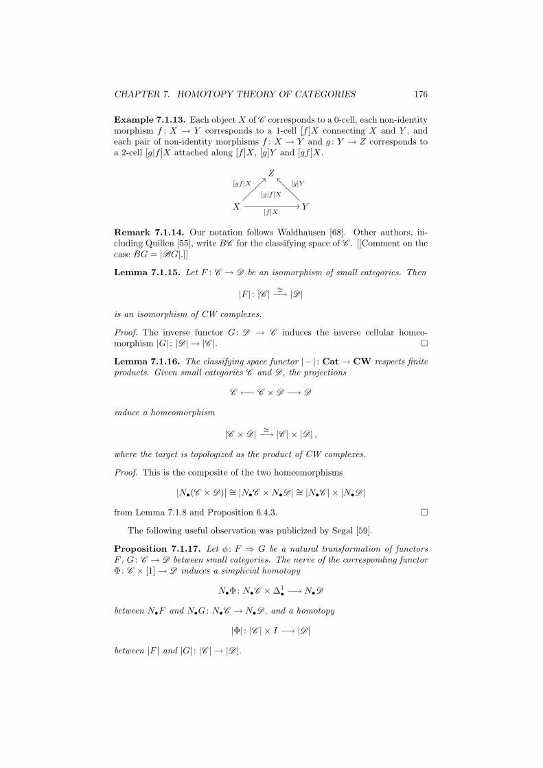
CHAPTER 7. HOMOTOPY THEORY OF CATEGORIES 176
Example 7.1.13. Each object X of C corresponds to a 0-cell, each non-identitymorphism f : X → Y corresponds to a 1-cell [f ]X connecting X and Y , andeach pair of non-identity morphisms f : X → Y and g : Y → Z corresponds toa 2-cell [g|f ]X attached along [f ]X, [g]Y and [gf ]X.
Z
X[f ]X
//
[gf ]X>>~~~~~~~ [g|f ]X
Y
[g]Y__@@@@@@@
Remark 7.1.14. Our notation follows Waldhausen [68]. Other authors, in-cluding Quillen [55], write BC for the classifying space of C . [[Comment on thecase BG = |BG|.]]
Lemma 7.1.15. Let F : C → D be an isomorphism of small categories. Then
|F | : |C |∼=−→ |D |
is an isomorphism of CW complexes.
Proof. The inverse functor G : D → C induces the inverse cellular homeo-morphism |G| : |D | → |C |.
Lemma 7.1.16. The classifying space functor |− | : Cat → CW respects finiteproducts. Given small categories C and D , the projections
C ←− C × D −→ D
induce a homeomorphism
|C × D |∼=−→ |C | × |D | ,
where the target is topologized as the product of CW complexes.
Proof. This is the composite of the two homeomorphisms
|N•(C × D)| ∼= |N•C × N•D | ∼= |N•C | × |N•D |
from Lemma 7.1.8 and Proposition 6.4.3.
The following useful observation was publicized by Segal [59].
Proposition 7.1.17. Let φ : F ⇒ G be a natural transformation of functorsF , G : C → D between small categories. The nerve of the corresponding functorΦ: C × [1] → D induces a simplicial homotopy
N•Φ: N•C × ∆1• −→ N•D
between N•F and N•G : N•C → N•D , and a homotopy
|Φ| : |C | × I −→ |D |
between |F | and |G| : |C | → |D |.
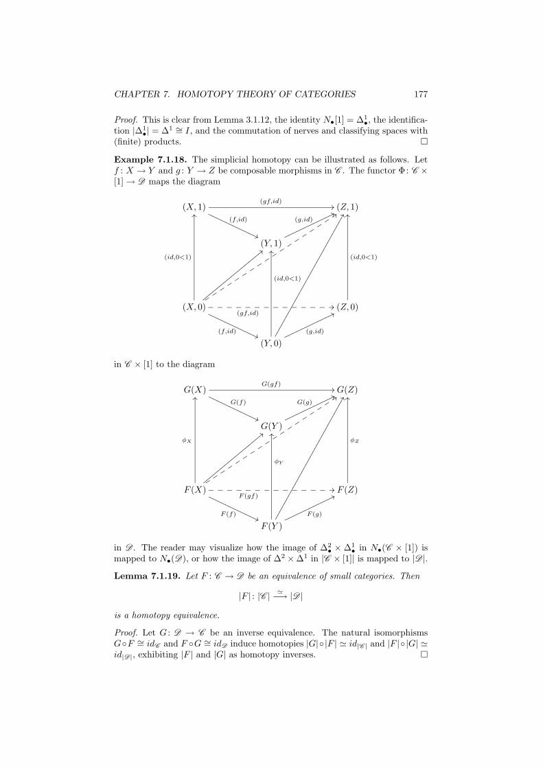
CHAPTER 7. HOMOTOPY THEORY OF CATEGORIES 177
Proof. This is clear from Lemma 3.1.12, the identity N•[1] = ∆1•, the identifica-
tion |∆1•| = ∆1 ∼= I, and the commutation of nerves and classifying spaces with
(finite) products.
Example 7.1.18. The simplicial homotopy can be illustrated as follows. Letf : X → Y and g : Y → Z be composable morphisms in C . The functor Φ: C ×[1] → D maps the diagram
(X, 1)(gf,id)
//
(f,id)
''PPPPPPPPPPPP(Z, 1)
(Y, 1)
(g,id)77nnnnnnnnnnnn
(X, 0)(gf,id)
//______________
(f,id)''PPPPPPPPPPPP
<<yyyyyyyyyyyyyyyyy
(id,0<1)
OO 99tt
tt
tt
tt
tt
tt
tt
tt
tt
(Z, 0)
(id,0<1)
OO
(Y, 0)
(g,id)
77nnnnnnnnnnnn
(id,0<1)
OO
FF°°°°°°°°°°°°°°°°°°°°°°°°°°°°°°°
in C × [1] to the diagram
G(X)G(gf)
//
G(f)
''PPPPPPPPPPPP G(Z)
G(Y )
G(g)77nnnnnnnnnnnn
F (X)F (gf)
//______________
F (f)''PPPPPPPPPPPP
<<zzzzzzzzzzzzzzzzz
φX
OO ::tt
tt
tt
tt
tt
tt
tt
tt
tt
F (Z)
φZ
OO
F (Y )
F (g)
77nnnnnnnnnnnn
φY
OO
FF°°°°°°°°°°°°°°°°°°°°°°°°°°°°°°°
in D . The reader may visualize how the image of ∆2• × ∆1
• in N•(C × [1]) ismapped to N•(D), or how the image of ∆2 × ∆1 in |C × [1]| is mapped to |D |.
Lemma 7.1.19. Let F : C → D be an equivalence of small categories. Then
|F | : |C |≃−→ |D |
is a homotopy equivalence.
Proof. Let G : D → C be an inverse equivalence. The natural isomorphismsGF ∼= idC and F G ∼= idD induce homotopies |G| |F | ≃ id|C | and |F | |G| ≃id|D|, exhibiting |F | and |G| as homotopy inverses.
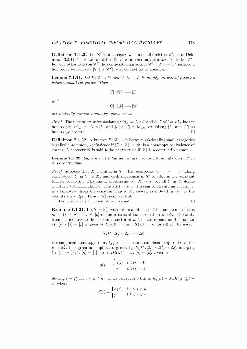
CHAPTER 7. HOMOTOPY THEORY OF CATEGORIES 178
Definition 7.1.20. Let C be a category with a small skeleton C ′, as in Defi-nition 3.2.11. Then we can define |C |, up to homotopy equivalence, to be |C ′|.For any other skeleton C ′′ the composite equivalence C ′ ⊆ C −→ C ′′ induces ahomotopy equivalence |C ′| ≃ |C ′′|, well-defined up to homotopy.
Lemma 7.1.21. Let F : C → D and G : D → C be an adjoint pair of functorsbetween small categories. Then
|F | : |C |≃−→ |D |
and|G| : |D |
≃−→ |C |
are mutually inverse homotopy equivalences.
Proof. The natural transformations η : idC ⇒ GF and ǫ : F G ⇒ idD inducehomotopies id|C | ≃ |G| |F | and |F | |G| ≃ id|D|, exhibiting |F | and |G| ashomotopy inverses.
Definition 7.1.22. A functor F : C → D between (skeletally) small categoriesis called a homotopy equivalence if |F | : |C | → |D | is a homotopy equivalence ofspaces. A category C is said to be contractible if |C | is a contractible space.
Lemma 7.1.23. Suppose that C has an initial object or a terminal object. ThenC is contractible.
Proof. Suppose that X is initial in C . The composite C → ∗ → C takingeach object Y in C to X, and each morphism in C to idX , is the constantfunctor const(X). The unique morphisms ǫY : X → Y , for all Y in C , definea natural transformation ǫ : const(X) ⇒ idC . Passing to classifying spaces, |ǫ|is a homotopy from the constant map to X, viewed as a 0-cell in |C |, to theidentity map id|C |. Hence |C | is contractible.
The case with a terminal object is dual.
Example 7.1.24. Let C = [p], with terminal object p. The unique morphismsηi = (i ≤ p) for i ∈ [p] define a natural transformation η : id[p] ⇒ constp
from the identity to the constant functor at p. The corresponding (bi-)functorH : [p] × [1] → [p] is given by H(i, 0) = i and H(i, 1) = p, for i ∈ [p]. Its nerve
N•H : ∆p• × ∆1
• −→ ∆p•
is a simplicial homotopy from id∆p•
to the constant simplicial map to the vertexp in ∆p
•. It is given in simplicial degree n by NnH : ∆pn × ∆1
n → ∆pn, mapping
(α : [n] → [p], ζ : [n] → [1]) to NnH(α, ζ) = β : [n] → [p], given by
β(i) =
α(i) if ζ(i) = 0
p if ζ(i) = 1.
Setting ζ = ζnk for 0 ≤ k ≤ n + 1, we can rewrite this as hk
n(α) = NnH(α, ζnk ) =
β, where
β(i) =
α(i) if 0 ≤ i < k
p if k ≤ i ≤ n.
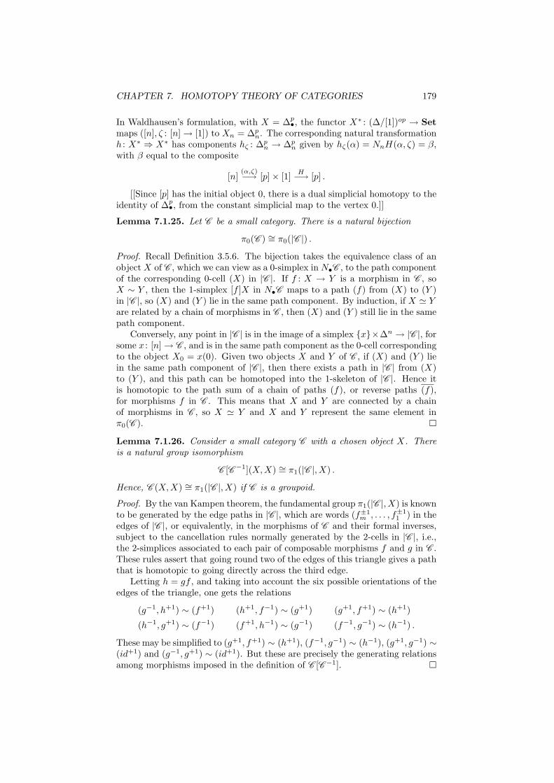
CHAPTER 7. HOMOTOPY THEORY OF CATEGORIES 179
In Waldhausen’s formulation, with X = ∆p•, the functor X∗ : (∆/[1])op → Set
maps ([n], ζ : [n] → [1]) to Xn = ∆pn. The corresponding natural transformation
h : X∗ ⇒ X∗ has components hζ : ∆pn → ∆p
n given by hζ(α) = NnH(α, ζ) = β,with β equal to the composite
[n](α,ζ)−→ [p] × [1]
H−→ [p] .
[[Since [p] has the initial object 0, there is a dual simplicial homotopy to theidentity of ∆p
•, from the constant simplicial map to the vertex 0.]]
Lemma 7.1.25. Let C be a small category. There is a natural bijection
π0(C ) ∼= π0(|C |) .
Proof. Recall Definition 3.5.6. The bijection takes the equivalence class of anobject X of C , which we can view as a 0-simplex in N•C , to the path componentof the corresponding 0-cell (X) in |C |. If f : X → Y is a morphism in C , soX ∼ Y , then the 1-simplex [f ]X in N•C maps to a path (f) from (X) to (Y )in |C |, so (X) and (Y ) lie in the same path component. By induction, if X ≃ Yare related by a chain of morphisms in C , then (X) and (Y ) still lie in the samepath component.
Conversely, any point in |C | is in the image of a simplex x×∆n → |C |, forsome x : [n] → C , and is in the same path component as the 0-cell correspondingto the object X0 = x(0). Given two objects X and Y of C , if (X) and (Y ) liein the same path component of |C |, then there exists a path in |C | from (X)to (Y ), and this path can be homotoped into the 1-skeleton of |C |. Hence itis homotopic to the path sum of a chain of paths (f), or reverse paths (f),for morphisms f in C . This means that X and Y are connected by a chainof morphisms in C , so X ≃ Y and X and Y represent the same element inπ0(C ).
Lemma 7.1.26. Consider a small category C with a chosen object X. Thereis a natural group isomorphism
C [C−1](X,X) ∼= π1(|C |,X) .
Hence, C (X,X) ∼= π1(|C |,X) if C is a groupoid.
Proof. By the van Kampen theorem, the fundamental group π1(|C |,X) is knownto be generated by the edge paths in |C |, which are words (f±1
m , . . . , f±11 ) in the
edges of |C |, or equivalently, in the morphisms of C and their formal inverses,subject to the cancellation rules normally generated by the 2-cells in |C |, i.e.,the 2-simplices associated to each pair of composable morphisms f and g in C .These rules assert that going round two of the edges of this triangle gives a paththat is homotopic to going directly across the third edge.
Letting h = gf , and taking into account the six possible orientations of theedges of the triangle, one gets the relations
(g−1, h+1) ∼ (f+1) (h+1, f−1) ∼ (g+1) (g+1, f+1) ∼ (h+1)
(h−1, g+1) ∼ (f−1) (f+1, h−1) ∼ (g−1) (f−1, g−1) ∼ (h−1) .
These may be simplified to (g+1, f+1) ∼ (h+1), (f−1, g−1) ∼ (h−1), (g+1, g−1) ∼(id+1) and (g−1, g+1) ∼ (id+1). But these are precisely the generating relationsamong morphisms imposed in the definition of C [C−1].
CHAPTER 7. HOMOTOPY THEORY OF CATEGORIES 180
7.2 The bar construction
Definition 7.2.1. Let M be a monoid with unit element e and multiplicationµ : M × M → M taking (m,m′) to µ(m,m′) = mm′. Let BM be the categorywith one object ∗, and one morphism [m] : ∗ → ∗ for each m ∈ M , with identity[e], and composition [m] · [m′] = [mm′] for m,m′ ∈ M . The simplicial barconstruction on M is the nerve
B•M = N•BM .
It is the simplicial set with n-simplices the set
BnM = [mn| . . . |m1] | mi ∈ M = Mn ,
face maps di : BnM → Bn−1M given by
di([mn| . . . |m1]) =
[mn| . . . |m2] for i = 0,
[mn| . . . |mi+1mi| . . . |m1] for 0 < i < n,
[mn−1| . . . |m1] for i = n,
and degeneracy maps sj : BnM → Bn+1M given by
sj([mn| . . . |m1) = [mn| . . . |mj+1|e|mj | . . . |m1]
for 0 ≤ j ≤ n. The bar construction on M is the topological realization
BM = |B•M | = |BM | .
It is a CW complex with one n-cell [mn| . . . |m1] for each n-tuple of non-identityelements in M .
Given a monoid homomorphism f : M → N , let B•f : B•M → B•N be thesimplicial map of nerves B•f = N•(Bf), given in degree n by
(Bnf)([mn| . . . |m1]) = [f(mn)| . . . |f(m1)] .
Let Bf : BM → BN be the cellular map Bf = |B•f | = |Bf |.
Example 7.2.2. The bar construction on the trivial monoid e is a point.The bar construction BC2 on a group with two elements e, T has one n-cell[T | . . . |T ] for each n ≥ 0.
Lemma 7.2.3. The composite B• = N•B : Mon → sSet is a full and faithfulfunctor, and B = | − | B• : Mon → CW is a (faithful) functor.
Proof. This is clear from Lemmas 2.8.5, 6.3.26 and 7.1.6.
Lemma 7.2.4. The projections M ← M ×N → N induce a natural simplicialisomorphism
B•(M × N)∼=−→ B•M × B•N
and a natural homeomorphism of CW complexes
B(M × N)∼=−→ BM × BN .
CHAPTER 7. HOMOTOPY THEORY OF CATEGORIES 181
Proof. This is clear from Lemmas 2.8.7 and 7.1.16.
Lemma 7.2.5. If M is commutative, then the unit map e → M and themultiplication map µ : M ×M → M induce simplicial maps ∗ = B•e → B•Mand
B•µ : B•M × B•M ∼= B•(M × M) −→ B•M ,
making B•M a commutative monoid in sSet. Passing to CW realizations, themaps ∗ → BM and
Bµ : BM × BM ∼= B(M × M) −→ BM
make BM a commutative monoid in CW.
[[Proof]][[Can iterate, to form BnM .]]
Definition 7.2.6 (Translation category). Let M be a monoid and Y a leftM -set. Let B(M,Y ) be the small category with objects the y ∈ Y , and witha morphism [m]y from y to my for each m ∈ M , y ∈ Y . We call B(M,Y ) thetranslation category of the M -action on Y . If M = G is a group, then B(G,Y )is a groupoid, called the translation groupoid.
Definition 7.2.7. In the special case Y = M , let E (M) = B(M,M) be thetranslation category for M acting from the left on itself, and let EM = |E (M)|be its classifying space. The right action of M on Y = M induces a rightaction on E (M) and on EM . [[Free action when M = G is a group, withorbits EG/G = BG.]] Note that E (M) has the initial object e, with a uniquemorphism [m]e from e to any other object m. Hence EM is contractible.
Lemma 7.2.8. |B(M,Y )| ∼= EM ×M Y . When M = G is a group, there is afiber bundle Y → EG ×G Y → BG.
[[Same for simplicial monoids/groups acting on simplicial sets.]][[One-sided bar construction. E•G = B•(∗, G,G) contractible. fiber se-
quence G → EG → BG.]][[Form two-sided bar construction B(X,M, Y ) as classifying space of the
category with objects X × Y and a morphism from (x · m, y) to (x,m · y), orvice versa.]]
Definition 7.2.9. Let M be a monoid, X a right M -set and Y a left M -set.Let B(X,M, Y ) be the small category with objects the pairs (x, y) ∈ X × Y ,and one morphism x[m]y from (xm, y) to (x,my) for each x ∈ X, m ∈ M andy ∈ Y . The composite of x[m]y and [[ETC]]
[[Compute π0 and π1 of |C |, at least for groupoids.]]
7.3 Quillen’s theorem A
Quillen [55, p. 93] found the following useful sufficient condition for a functorto be a homotopy equivalence.
Theorem 7.3.1 (Quillen’s theorem A). Let F : C → D be a functor of smallcategories. Suppose that the left fiber F/Y is contractible for each object Y ofD . Then F is a homotopy equivalence.
CHAPTER 7. HOMOTOPY THEORY OF CATEGORIES 182
Proof. Let T•,•(F ) be the bisimplicial set with (m,n)-bisimplices the diagrams
X0// . . . // Xm_
²²
F (Xm)f
// Y0// . . . // Yn
where the upper row lies in C and the lower row lies in D . In other words,an element of Tm,n(F ) is a triple (x, f, y), where x : [m] → C , y : [n] → D andf : F (Xm) → Y0 is a morphism in D , where we set Xi = x(i) and Yj = y(j) fori ∈ [m], j ∈ [n].
The bisimplicial structure map (α, β)∗, for α : [p] → [m], β : [q] → [n], takes(x, f, y) to
(α, β)∗(x, f, y) = (α∗(x), g, β∗(y))
in Tp,q(F ), where g : F (α∗(x)p) → β∗(y)0 is the composite
F (Xα(p)) −→ F (Xm)f
−→ Y0 −→ Yβ(0) .
Hence the i-th left hand face map deletes Xi, and replaces F (Xm) → Y0 with thecomposite F (Xm−1) → F (Xm) → Y0 if i = m. The j-th left hand degeneracymap repeats Xj . The i-th right hand face map deletes Yi, and replaces F (Xm) →Y0 with the composite F (Xm) → Y0 → Y1 if i = 0. The j-th right handdegeneracy map repeats Yj .
For each m ≥ 0, the simplicial set Tm,•(F ) decomposes as the disjoint union
Tm,•(F ) ∼=∐
x∈NmC
N•(F (Xm)/D) .
indexed on the x : [m] → C . Each category F (Xm)/D has an initial object,hence is contractible by Lemma 7.1.23. Thus the simplicial map
sm,• : Tm,•(F ) ∼=∐
x∈NmC
N•(F (Xm)/D)≃−→
∐
x∈NmC
∗ ∼= NmC
collapsing each summand N•(F (Xm)/D) to a point ∗ ∼= ∆0•, is a weak homotopy
equivalence. Here the set NmC is viewed as a simplicial set in a trivial way,with n-simplices NmC for all n ≥ 0, and identity maps as simplicial structuremaps.
Likewise, we view N•C as a bisimplicial set in a trivial way, with (m,n)-simplices NmC for all m,n ≥ 0. In functorial terms, we are considering thecomposite functor
∆op × ∆op pr1−→ ∆op N•C
−→ Set .
The weak homotopy equivalences sm,• : Tm,•(F ) → NmC for m ≥ 0 combine toa bisimplicial map
s•,• : T•,•(F )≃−→ N•C .
By the realization lemma, s•,• is a weak homotopy equivalence.On the other hand, for each n ≥ 0, the simplicial set T•,n(F ) decomposes as
the disjoint union
T•,n(F ) ∼=∐
y∈NnD
N•(F/Y0)
CHAPTER 7. HOMOTOPY THEORY OF CATEGORIES 183
indexed on the y : [n] → D . By hypothesis, each left fiber category F/Y0 iscontractible. Thus the simplicial map
t•,n : T•,n(F ) ∼=∐
y∈NnD
N•(F/Y0)≃−→
∐
y∈NnD
∗ ∼= NnD
collapsing each summand N•(F/Y0) to a point, is a weak homotopy equivalence.Now we view N•D as a bisimplicial set in the “other” trivial way, with
(m,n)-simplices NnD for all m,n ≥ 0. The weak homotopy equivalences t•,n
combine to a bisimplicial map
t•,• : T•,•(F )≃−→ N•D .
By the realization lemma, in its reflected form, t•,• is a weak homotopy equiv-alence.
Note that the maps s•,• and t•,• are natural in F , in the sense that thediagram
N•C
N•F
²²
T•,•(F )s•,•
≃oo
²²
t•,•
≃// N•D
=
²²
N•D T•,•(idD)s•,•
≃oot•,•
≃ // N•D
commutes. The middle vertical map takes (x, f, y) in Tm,n(F ) to (F x, f, y) inTm,n(idD), realized by the diagram
F (X0) // . . . // F (Xm)_
²²
F (Xm)f
// Y0// . . . // Yn .
It is clear that each left fiber idD/Y is contractible, as this is the same as theovercategory D/Y , with the terminal object id : Y → Y . Hence the argumentsabove, for idD in place of F , show that also the lower maps s•,• and t•,• areweak homotopy equivalences.
Chasing the diagram, it follows that N•F is a weak homotopy equivalence,so F : C → D is a homotopy equivalence.
Corollary 7.3.2. Let F : C → D be a functor of small categories. Supposethat the right fiber Y/F is contractible for each object Y of D . Then F is ahomotopy equivalence.
Proof. This is clear from the other form of Quillen’s theorem A by duality.
Recall Definitions 4.4.1 and 4.4.2.
Corollary 7.3.3. Let C be a precofibered (or prefibered) category over D , viaa functor F : C → D , and that the fiber F−1(Y ) is contractible for each objectY of D . Then F is a homotopy equivalence.
Proof. This is clear by the assumed existence of a left adjoint to F−1(Y ) → F/Y(or right adjoint to F−1(Y ) → Y/F ), Lemma 7.1.21 and Quillen’s theorem A.
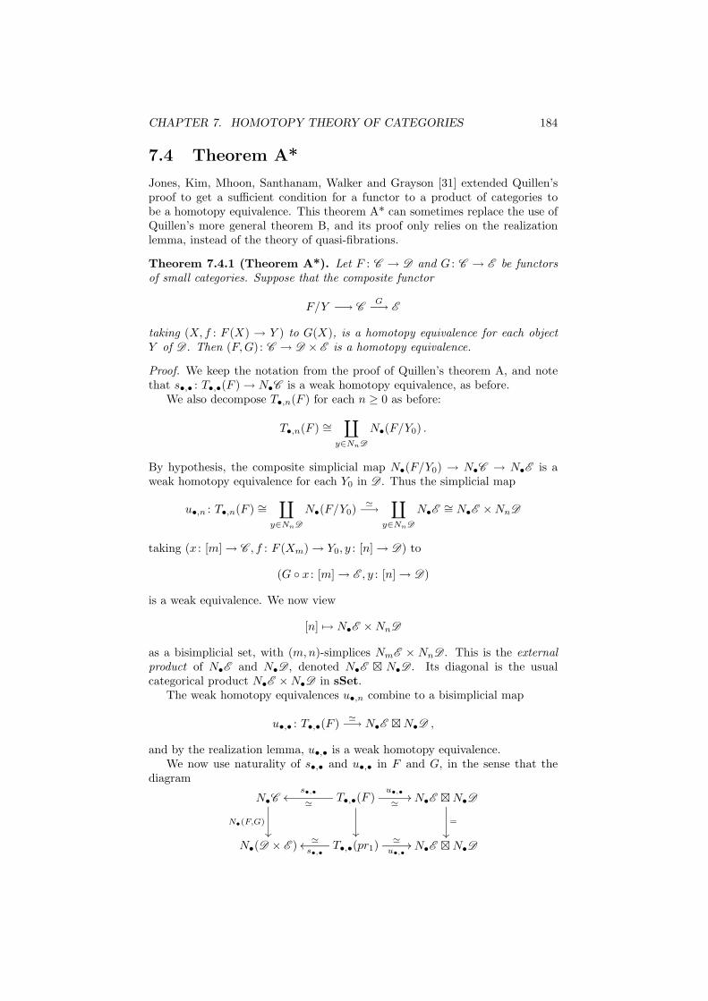
CHAPTER 7. HOMOTOPY THEORY OF CATEGORIES 184
7.4 Theorem A*
Jones, Kim, Mhoon, Santhanam, Walker and Grayson [31] extended Quillen’sproof to get a sufficient condition for a functor to a product of categories tobe a homotopy equivalence. This theorem A* can sometimes replace the use ofQuillen’s more general theorem B, and its proof only relies on the realizationlemma, instead of the theory of quasi-fibrations.
Theorem 7.4.1 (Theorem A*). Let F : C → D and G : C → E be functorsof small categories. Suppose that the composite functor
F/Y −→ CG−→ E
taking (X, f : F (X) → Y ) to G(X), is a homotopy equivalence for each objectY of D . Then (F,G) : C → D × E is a homotopy equivalence.
Proof. We keep the notation from the proof of Quillen’s theorem A, and notethat s•,• : T•,•(F ) → N•C is a weak homotopy equivalence, as before.
We also decompose T•,n(F ) for each n ≥ 0 as before:
T•,n(F ) ∼=∐
y∈NnD
N•(F/Y0) .
By hypothesis, the composite simplicial map N•(F/Y0) → N•C → N•E is aweak homotopy equivalence for each Y0 in D . Thus the simplicial map
u•,n : T•,n(F ) ∼=∐
y∈NnD
N•(F/Y0)≃−→
∐
y∈NnD
N•E∼= N•E × NnD
taking (x : [m] → C , f : F (Xm) → Y0, y : [n] → D) to
(G x : [m] → E , y : [n] → D)
is a weak equivalence. We now view
[n] 7→ N•E × NnD
as a bisimplicial set, with (m,n)-simplices NmE × NnD . This is the externalproduct of N•E and N•D , denoted N•E ⊠ N•D . Its diagonal is the usualcategorical product N•E × N•D in sSet.
The weak homotopy equivalences u•,n combine to a bisimplicial map
u•,• : T•,•(F )≃−→ N•E ⊠ N•D ,
and by the realization lemma, u•,• is a weak homotopy equivalence.We now use naturality of s•,• and u•,• in F and G, in the sense that the
diagram
N•C
N•(F,G)
²²
T•,•(F )s•,•
≃oo
²²
u•,•
≃// N•E ⊠ N•D
=
²²
N•(D × E ) T•,•(pr1)s•,•
≃oou•,•
≃ // N•E ⊠ N•D
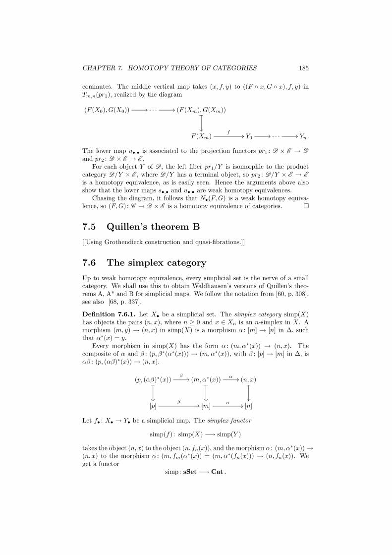
CHAPTER 7. HOMOTOPY THEORY OF CATEGORIES 185
commutes. The middle vertical map takes (x, f, y) to ((F x,G x), f, y) inTm,n(pr1), realized by the diagram
(F (X0), G(X0)) // . . . // (F (Xm), G(Xm))_
²²
F (Xm)f
// Y0// . . . // Yn .
The lower map u•,• is associated to the projection functors pr1 : D × E → D
and pr2 : D × E → E .For each object Y of D , the left fiber pr1/Y is isomorphic to the product
category D/Y × E , where D/Y has a terminal object, so pr2 : D/Y × E → E
is a homotopy equivalence, as is easily seen. Hence the arguments above alsoshow that the lower maps s•,• and u•,• are weak homotopy equivalences.
Chasing the diagram, it follows that N•(F,G) is a weak homotopy equiva-lence, so (F,G) : C → D × E is a homotopy equivalence of categories.
7.5 Quillen’s theorem B
[[Using Grothendieck construction and quasi-fibrations.]]
7.6 The simplex category
Up to weak homotopy equivalence, every simplicial set is the nerve of a smallcategory. We shall use this to obtain Waldhausen’s versions of Quillen’s theo-rems A, A* and B for simplicial maps. We follow the notation from [60, p. 308],see also [68, p. 337].
Definition 7.6.1. Let X• be a simplicial set. The simplex category simp(X)has objects the pairs (n, x), where n ≥ 0 and x ∈ Xn is an n-simplex in X. Amorphism (m, y) → (n, x) in simp(X) is a morphism α : [m] → [n] in ∆, suchthat α∗(x) = y.
Every morphism in simp(X) has the form α : (m,α∗(x)) → (n, x). Thecomposite of α and β : (p, β∗(α∗(x))) → (m,α∗(x)), with β : [p] → [m] in ∆, isαβ : (p, (αβ)∗(x)) → (n, x).
(p, (αβ)∗(x))_
²²
β// (m,α∗(x))
_
²²
α // (n, x)_
²²
[p]β
// [m]α // [n]
Let f• : X• → Y• be a simplicial map. The simplex functor
simp(f) : simp(X) −→ simp(Y )
takes the object (n, x) to the object (n, fn(x)), and the morphism α : (m,α∗(x)) →(n, x) to the morphism α : (m, fm(α∗(x)) = (m,α∗(fn(x))) → (n, fn(x)). Weget a functor
simp: sSet −→ Cat .
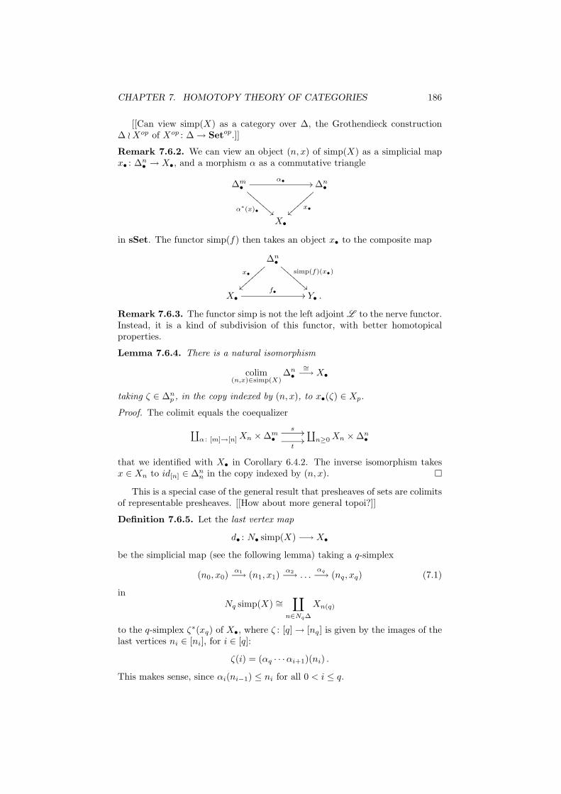
CHAPTER 7. HOMOTOPY THEORY OF CATEGORIES 186
[[Can view simp(X) as a category over ∆, the Grothendieck construction∆ ≀ Xop of Xop : ∆ → Setop.]]
Remark 7.6.2. We can view an object (n, x) of simp(X) as a simplicial mapx• : ∆n
• → X•, and a morphism α as a commutative triangle
∆m•
α• //
α∗(x)• !!CCCC
CCCC
∆n•
x•
||||
||||
X•
in sSet. The functor simp(f) then takes an object x• to the composite map
∆n•
x•
||||
|||| simp(f)(x•)
!!CCCC
CCCC
X•f• // Y• .
Remark 7.6.3. The functor simp is not the left adjoint L to the nerve functor.Instead, it is a kind of subdivision of this functor, with better homotopicalproperties.
Lemma 7.6.4. There is a natural isomorphism
colim(n,x)∈simp(X)
∆n•
∼=−→ X•
taking ζ ∈ ∆np , in the copy indexed by (n, x), to x•(ζ) ∈ Xp.
Proof. The colimit equals the coequalizer
∐α : [m]→[n] Xn × ∆m
•
s //
t//
∐n≥0 Xn × ∆n
•
that we identified with X• in Corollary 6.4.2. The inverse isomorphism takesx ∈ Xn to id[n] ∈ ∆n
n in the copy indexed by (n, x).
This is a special case of the general result that presheaves of sets are colimitsof representable presheaves. [[How about more general topoi?]]
Definition 7.6.5. Let the last vertex map
d• : N• simp(X) −→ X•
be the simplicial map (see the following lemma) taking a q-simplex
(n0, x0)α1−→ (n1, x1)
α2−→ . . .αq−→ (nq, xq) (7.1)
inNq simp(X) ∼=
∐
n∈Nq∆
Xn(q)
to the q-simplex ζ∗(xq) of X•, where ζ : [q] → [nq] is given by the images of thelast vertices ni ∈ [ni], for i ∈ [q]:
ζ(i) = (αq · · ·αi+1)(ni) .
This makes sense, since αi(ni−1) ≤ ni for all 0 < i ≤ q.
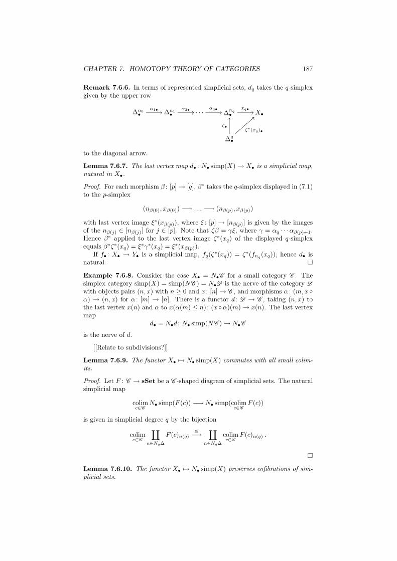
CHAPTER 7. HOMOTOPY THEORY OF CATEGORIES 187
Remark 7.6.6. In terms of represented simplicial sets, dq takes the q-simplexgiven by the upper row
∆n0•
α1• // ∆n1•
α2• // . . .αq•
// ∆nq•
xq•// X•
∆q•
ζ•
OO
ζ∗(xq)•
==
to the diagonal arrow.
Lemma 7.6.7. The last vertex map d• : N• simp(X) → X• is a simplicial map,natural in X•.
Proof. For each morphism β : [p] → [q], β∗ takes the q-simplex displayed in (7.1)to the p-simplex
(nβ(0), xβ(0)) −→ . . . −→ (nβ(p), xβ(p))
with last vertex image ξ∗(xβ(p)), where ξ : [p] → [nβ(p)] is given by the imagesof the nβ(j) ∈ [nβ(j)] for j ∈ [p]. Note that ζβ = γξ, where γ = αq · · ·αβ(p)+1.Hence β∗ applied to the last vertex image ζ∗(xq) of the displayed q-simplexequals β∗ζ∗(xq) = ξ∗γ∗(xq) = ξ∗(xβ(p)).
If f• : X• → Y• is a simplicial map, fq(ζ∗(xq)) = ζ∗(fnq
(xq)), hence d• isnatural.
Example 7.6.8. Consider the case X• = N•C for a small category C . Thesimplex category simp(X) = simp(NC ) = N•D is the nerve of the category D
with objects pairs (n, x) with n ≥ 0 and x : [n] → C , and morphisms α : (m,x α) → (n, x) for α : [m] → [n]. There is a functor d : D → C , taking (n, x) tothe last vertex x(n) and α to x(α(m) ≤ n) : (x α)(m) → x(n). The last vertexmap
d• = N•d : N• simp(NC ) → N•C
is the nerve of d.
[[Relate to subdivisions?]]
Lemma 7.6.9. The functor X• 7→ N• simp(X) commutes with all small colim-its.
Proof. Let F : C → sSet be a C -shaped diagram of simplicial sets. The naturalsimplicial map
colimc∈C
N• simp(F (c)) −→ N• simp(colimc∈C
F (c))
is given in simplicial degree q by the bijection
colimc∈C
∐
n∈Nq∆
F (c)n(q)
∼=−→
∐
n∈Nq∆
colimc∈C
F (c)n(q) .
Lemma 7.6.10. The functor X• 7→ N• simp(X) preserves cofibrations of sim-plicial sets.
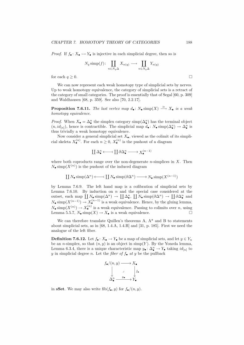
CHAPTER 7. HOMOTOPY THEORY OF CATEGORIES 188
Proof. If f• : X• Y• is injective in each simplicial degree, then so is
Nq simp(f) :∐
n∈Nq∆
Xn(q) −→∐
n∈Nq∆
Yn(q)
for each q ≥ 0.
We can now represent each weak homotopy type of simplicial sets by nerves.Up to weak homotopy equivalence, the category of simplicial sets is a retract ofthe category of small categories. The proof is essentially that of Segal [60, p. 309]and Waldhausen [68, p. 359]. See also [70, 2.2.17].
Proposition 7.6.11. The last vertex map d• : N• simp(X)≃−→ X• is a weak
homotopy equivalence.
Proof. When X• = ∆n• the simplex category simp(∆n
• ) has the terminal object(n, id[n]), hence is contractible. The simplicial map d• : N• simp(∆n
• ) → ∆n• is
thus trivially a weak homotopy equivalence.Now consider a general simplicial set X•, viewed as the colimit of its simpli-
cial skeleta X(n)• . For each n ≥ 0, X
(n)• is the pushout of a diagram
∐∆n
•
∐∂∆n
•oooo // X
(n−1)•
where both coproducts range over the non-degenerate n-simplices in X. ThenN• simp(X(n)) is the pushout of the induced diagram
∐N• simp(∆n)
∐N• simp(∂∆n)oooo // N• simp(X(n−1))
by Lemma 7.6.9. The left hand map is a cofibration of simplicial sets byLemma 7.6.10. By induction on n and the special case considered at theoutset, each map
∐N• simp(∆n) →
∐∆n
• ,∐
N• simp(∂∆n) →∐
∂∆n• and
N• simp(X(n−1)) → X(n−1)• is a weak equivalence. Hence, by the gluing lemma,
N• simp(X(n)) → X(n)• is a weak equivalence. Passing to colimits over n, using
Lemma 5.5.7, N• simp(X) → X• is a weak equivalence.
We can therefore translate Quillen’s theorems A, A* and B to statementsabout simplicial sets, as in [68, 1.4.A, 1.4.B] and [31, p. 185]. First we need theanalogue of the left fiber.
Definition 7.6.12. Let f• : X• → Y• be a map of simplicial sets, and let y ∈ Yn
be an n-simplex, so that (n, y) is an object in simp(Y ). By the Yoneda lemma,Lemma 6.3.4, there is a unique characteristic map y• : ∆n
• → Y• taking id[n] toy in simplicial degree n. Let the fiber of f• at y be the pullback
f•/(n, y) //
²²
y
X•
f•
²²
∆n•
y• // Y•
in sSet. We may also write fib(f•, y) for f•/(n, y).
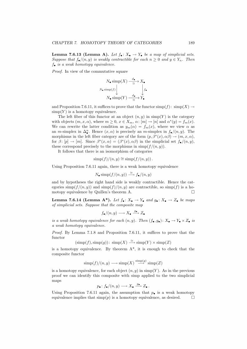
CHAPTER 7. HOMOTOPY THEORY OF CATEGORIES 189
Lemma 7.6.13 (Lemma A). Let f• : X• → Y• be a map of simplicial sets.Suppose that f•/(n, y) is weakly contractible for each n ≥ 0 and y ∈ Yn. Thenf• is a weak homotopy equivalence.
Proof. In view of the commutative square
N• simp(X)d•
≃//
N• simp(f)
²²
X•
f•
²²
N• simp(Y )d•
≃// Y•
and Proposition 7.6.11, it suffices to prove that the functor simp(f) : simp(X) →simp(Y ) is a homotopy equivalence.
The left fiber of this functor at an object (n, y) in simp(Y ) is the categorywith objects (m,x, α), where m ≥ 0, x ∈ Xm, α : [m] → [n] and α∗(y) = fm(x).We can rewrite the latter condition as ym(α) = fm(x), where we view α asan m-simplex in ∆n
• . Hence (x, α) is precisely an m-simplex in f•/(n, y). Themorphisms in the left fiber category are of the form (p, β∗(x), αβ) → (m,x, α),for β : [p] → [m]. Since β∗(x, α) = (β∗(x), αβ) in the simplicial set f•/(n, y),these correspond precisely to the morphisms in simp(f/(n, y)).
It follows that there is an isomorphism of categories
simp(f)/(n, y) ∼= simp(f/(n, y)) .
Using Proposition 7.6.11 again, there is a weak homotopy equivalence
N• simp(f/(n, y))≃−→ f•/(n, y)
and by hypotheses the right hand side is weakly contractible. Hence the cat-egories simp(f/(n, y)) and simp(f)/(n, y) are contractible, so simp(f) is a ho-motopy equivalence by Quillen’s theorem A.
Lemma 7.6.14 (Lemma A*). Let f• : X• → Y• and g• : X• → Z• be mapsof simplicial sets. Suppose that the composite map
f•/(n, y) −→ X•g•−→ Z•
is a weak homotopy equivalence for each (n, y). Then (f•, g•) : X• → Y• ×Z• isa weak homotopy equivalence.
Proof. By Lemma 7.1.8 and Proposition 7.6.11, it suffices to prove that thefunctor
(simp(f), simp(g)) : simp(X)≃−→ simp(Y ) × simp(Z)
is a homotopy equivalence. By theorem A*, it is enough to check that thecomposite functor
simp(f)/(n, y) −→ simp(X)simp(g)−→ simp(Z)
is a homotopy equivalence, for each object (n, y) in simp(Y ). As in the previousproof we can identify this composite with simp applied to the two simplicialmaps
p• : f•/(n, y) −→ X•g•−→ Z• .
Using Proposition 7.6.11 again, the assumption that p• is a weak homotopyequivalence implies that simp(p) is a homotopy equivalence, as desired.
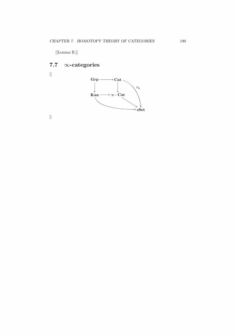
CHAPTER 7. HOMOTOPY THEORY OF CATEGORIES 190
[[Lemma B.]]
7.7 ∞-categories
[[
Grp //
²²
Cat
²²
N•
³³
Kan //
//
∞−Cat
%%KKKKKKKKK
sSet
]]
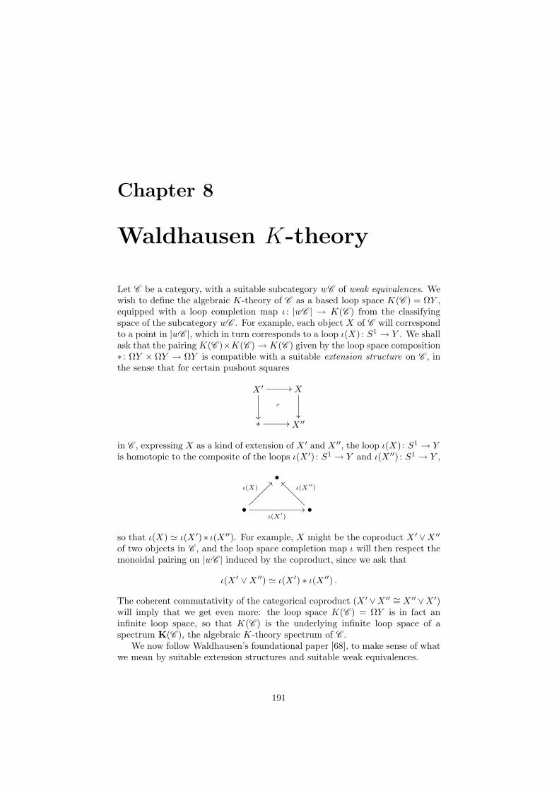
Chapter 8
Waldhausen K-theory
Let C be a category, with a suitable subcategory wC of weak equivalences. Wewish to define the algebraic K-theory of C as a based loop space K(C ) = ΩY ,equipped with a loop completion map ι : |wC | → K(C ) from the classifyingspace of the subcategory wC . For example, each object X of C will correspondto a point in |wC |, which in turn corresponds to a loop ι(X) : S1 → Y . We shallask that the pairing K(C )×K(C ) → K(C ) given by the loop space composition∗ : ΩY × ΩY → ΩY is compatible with a suitable extension structure on C , inthe sense that for certain pushout squares
X ′ //
²²
p
X
²²
∗ // X ′′
in C , expressing X as a kind of extension of X ′ and X ′′, the loop ι(X) : S1 → Yis homotopic to the composite of the loops ι(X ′) : S1 → Y and ι(X ′′) : S1 → Y ,
•
•ι(X′)
//
ι(X)??ÄÄÄÄÄÄÄ
•
ι(X′′)__@@@@@@@
so that ι(X) ≃ ι(X ′) ∗ ι(X ′′). For example, X might be the coproduct X ′ ∨X ′′
of two objects in C , and the loop space completion map ι will then respect themonoidal pairing on |wC | induced by the coproduct, since we ask that
ι(X ′ ∨ X ′′) ≃ ι(X ′) ∗ ι(X ′′) .
The coherent commutativity of the categorical coproduct (X ′ ∨X ′′ ∼= X ′′ ∨X ′)will imply that we get even more: the loop space K(C ) = ΩY is in fact aninfinite loop space, so that K(C ) is the underlying infinite loop space of aspectrum K(C ), the algebraic K-theory spectrum of C .
We now follow Waldhausen’s foundational paper [68], to make sense of whatwe mean by suitable extension structures and suitable weak equivalences.
191
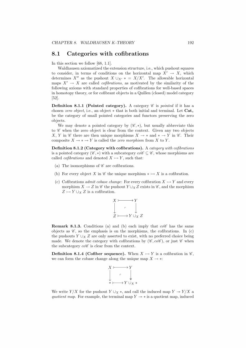
CHAPTER 8. WALDHAUSEN K-THEORY 192
8.1 Categories with cofibrations
In this section we follow [68, 1.1].Waldhausen axiomatized the extension structure, i.e., which pushout squares
to consider, in terms of conditions on the horizontal map X ′ → X, whichdetermines X ′′ as the pushout X ∪X′ ∗ = X/X ′. The allowable horizontalmaps X ′ → X are called cofibrations, as motivated by the similarity of thefollowing axioms with standard properties of cofibrations for well-based spacesin homotopy theory, or for cofibrant objects in a Quillen (closed) model category[52].
Definition 8.1.1 (Pointed category). A category C is pointed if it has achosen zero object, i.e., an object ∗ that is both initial and terminal. Let Cat∗be the category of small pointed categories and functors preserving the zeroobjects.
We may denote a pointed category by (C , ∗), but usually abbreviate thisto C when the zero object is clear from the context. Given any two objectsX, Y in C there are then unique morphisms X → ∗ and ∗ → Y in C . Theircomposite X → ∗ → Y is called the zero morphism from X to Y .
Definition 8.1.2 (Category with cofibrations). A category with cofibrationsis a pointed category (C , ∗) with a subcategory coC ⊆ C , whose morphisms arecalled cofibrations and denoted X Y , such that:
(a) The isomorphisms of C are cofibrations.
(b) For every object X in C the unique morphism ∗ X is a cofibration.
(c) Cofibrations admit cobase change: For every cofibration X Y and everymorphism X → Z in C the pushout Y ∪X Z exists in C , and the morphismZ Y ∪X Z is a cofibration.
X // //
²²
p
Y
²²
Z // // Y ∪X Z
Remark 8.1.3. Conditions (a) and (b) each imply that coC has the sameobjects as C , so the emphasis is on the morphisms, the cofibrations. In (c)the pushouts Y ∪X Z are only asserted to exist, with no preferred choice beingmade. We denote the category with cofibrations by (C , coC ), or just C whenthe subcategory coC is clear from the context.
Definition 8.1.4 (Cofiber sequence). When X Y is a cofibration in C ,we can form the cobase change along the unique map X → ∗:
X // //
²²
p
Y
²²²²
∗ // // Y ∪X ∗
We write Y/X for the pushout Y ∪X ∗, and call the induced map Y ։ Y/X aquotient map. For example, the terminal map Y ։ ∗ is a quotient map, induced
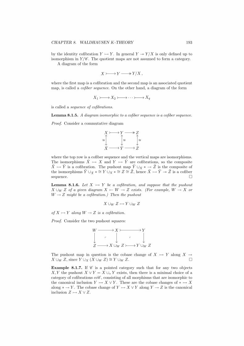
CHAPTER 8. WALDHAUSEN K-THEORY 193
by the identity cofibration Y Y . In general Y ։ Y/X is only defined up toisomorphism in Y/C . The quotient maps are not assumed to form a category.
A diagram of the form
X // // Y // // Y/X ,
where the first map is a cofibration and the second map is an associated quotientmap, is called a cofiber sequence. On the other hand, a diagram of the form
X1// // X2
// // . . . // // Xq
is called a sequence of cofibrations.
Lemma 8.1.5. A diagram isomorphic to a cofiber sequence is a cofiber sequence.
Proof. Consider a commutative diagram
X // //OO
∼=
²²
Y // //OO
∼=
²²
ZOO
∼=
²²
X // Y // Z
where the top row is a cofiber sequence and the vertical maps are isomorphisms.The isomorphisms X X and Y Y are cofibrations, so the compositeX Y is a cofibration. The pushout map Y ∪X ∗ → Z is the composite ofthe isomorphisms Y ∪X ∗ ∼= Y ∪X ∗ ∼= Z ∼= Z, hence X Y ։ Z is a cofibersequence.
Lemma 8.1.6. Let X Y be a cofibration, and suppose that the pushoutX ∪W Z of a given diagram X ← W → Z exists. (For example, W → X orW → Z might be a cofibration.) Then the pushout
X ∪W Z Y ∪W Z
of X Y along W → Z is a cofibration.
Proof. Consider the two pushout squares:
W //
²²
p
X // //
²²
p
Y
²²
Z // X ∪W Z // // Y ∪W Z
The pushout map in question is the cobase change of X Y along X →X ∪W Z, since Y ∪X (X ∪W Z) ∼= Y ∪W Z.
Example 8.1.7. If C is a pointed category such that for any two objectsX,Y the pushout X ∨ Y = X ∪∗ Y exists, then there is a minimal choice of acategory of cofibrations coC , consisting of all morphisms that are isomorphic tothe canonical inclusion Y X ∨ Y . These are the cobase changes of ∗ Xalong ∗ → Y . The cobase change of Y X ∨ Y along Y → Z is the canonicalinclusion Z X ∨ Z.
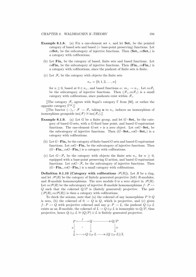
CHAPTER 8. WALDHAUSEN K-THEORY 194
Example 8.1.8. (a) Fix a one-element set ∗, and let Set∗ be the pointedcategory of based sets and based (= base-point preserving) functions. LetcoSet∗ be the subcategory of injective functions. Then (Set∗, coSet∗) isa category with cofibrations.
(b) Let Fin∗ be the category of based, finite sets and based functions. LetcoFin∗ be the subcategory of injective functions. Then (Fin∗, coFin∗) isa category with cofibrations, since the pushout of finite sets is finite.
(c) Let F∗ be the category with objects the finite sets
n+ = 0, 1, 2, . . . , n
for n ≥ 0, based at 0 ∈ n+, and based functions α : m+ → n+. Let coF∗
be the subcategory of injective functions. Then (F∗, coF∗) is a smallcategory with cofibrations, since pushouts exist within F∗.
[[The category F∗ agrees with Segal’s category Γ from [60], or rather theopposite category Γop.]]
[[The functor (−)+ : F → F∗ taking n to n+ induces an isomorphism ofisomorphism groupoids iso(F ) ∼= iso(F∗).]]
Example 8.1.9. (a) Let G be a finite group, and let G−Set∗ be the cate-gory of based G-sets, with a G-fixed base point, and based G-equivariantfunctions. The one-element G-set ∗ is a zero object. Let coG−Set∗ bethe subcategory of injective functions. Then (G−Set∗, coG−Set∗) is acategory with cofibrations.
(b) Let G−Fin∗ be the category of finite based G-sets and based G-equivariantfunctions. Let coG−Fin∗ be the subcategory of injective functions. Then(G−Fin∗, coG−Fin∗) is a category with cofibrations.
(c) Let G−F∗ be the category with objects the finite sets n+ for n ≥ 0,equipped with a base-point preserving G-action, and based G-equivariantfunctions. Let coG−F∗ be the subcategory of injective functions. Then(G−Fin∗, coG−Fin∗) is a small category with cofibrations.
Definition 8.1.10 (Category with cofibrations P(R)). Let R be a ring,and let P(R) be the category of finitely generated projective (left) R-modules,and R-module homomorphisms. The zero module 0 is a zero object in P(R).Let coP(R) be the subcategory of injective R-module homomorphisms f : P
Q such that the cokernel Q/P is (finitely generated) projective. The pair(P(R), coP(R)) is then a category with cofibrations.
To check the axioms, note that (a) the cokernel of any isomorphism P ∼= Qis zero, (b) the cokernel of 0 → Q is Q, which is projective, and (c) givenf : P Q with projective cokernel and any g : P → L, the pushout Q ⊕P Lexists as an R-module, the cokernel of L → Q⊕P L is isomorphic to Q/P , thusprojective, hence Q ⊕P L ∼= (Q/P ) ⊕ L is finitely generated projective.
P //f
//
g
²²
p
Q // //
²²
Q/P
∼=
²²
L // // Q ⊕P L // // (Q ⊕P L)/L
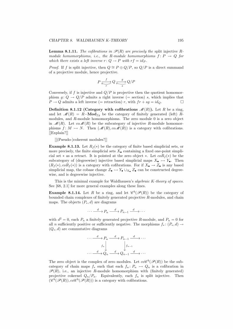
CHAPTER 8. WALDHAUSEN K-THEORY 195
Lemma 8.1.11. The cofibrations in P(R) are precisely the split injective R-module homomorphisms, i.e., the R-module homomorphisms f : P → Q forwhich there exists a left inverse r : Q → P with rf = idP .
Proof. If f is split injective, then Q ∼= P ⊕ Q/P , so Q/P is a direct summandof a projective module, hence projective.
Pf
// Qg
//
rii Q/P
s
ii
Conversely, if f is injective and Q/P is projective then the quotient homomor-phism g : Q → Q/P admits a right inverse (= section) s, which implies thatP → Q admits a left inverse (= retraction) r, with fr + sg = idQ.
Definition 8.1.12 (Category with cofibrations M (R)). Let R be a ring,and let M (R) = R−Modfg be the category of finitely generated (left) R-modules, and R-module homomorphisms. The zero module 0 is a zero objectin M (R). Let coM (R) be the subcategory of injective R-module homomor-phisms f : M N . Then (M (R), coM (R)) is a category with cofibrations.[[Explain?]]
[[(Pseudo-)coherent modules?]]
Example 8.1.13. Let Rf (∗) be the category of finite based simplicial sets, ormore precisely, the finite simplicial sets X• containing a fixed one-point simpli-cial set ∗ as a retract. It is pointed at the zero object ∗. Let coRf (∗) be thesubcategory of (degreewise) injective based simplicial maps X• Y•. Then(Rf (∗), coRf (∗)) is a category with cofibrations. For if X• → Z• is any basedsimplicial map, the cobase change Z• Y• ∪X•
Z• can be constructed degree-wise, and is degreewise injective.
This is the minimal example for Waldhausen’s algebraic K-theory of spaces.See [68, 2.1] for more general examples along these lines.
Example 8.1.14. Let R be a ring, and let C b(P(R)) be the category ofbounded chain complexes of finitely generated projective R-modules, and chainmaps. The objects (P∗, d) are diagrams
. . . d // Pnd // Pn−1
d // . . .
with d2 = 0, each Pn a finitely generated projective R-module, and Pn = 0 forall n sufficiently positive or sufficiently negative. The morphisms f∗ : (P∗, d) →(Q∗, d) are commutative diagrams
. . . d // Pnd //
fn
²²
Pn−1d //
fn−1
²²
. . .
. . . d // Qnd // Qn−1
d // . . .
The zero object is the complex of zero modules. Let coC b(P(R)) be the sub-category of chain maps f∗ such that each fn : Pn Qn is a cofibration inP(R), i.e., an injective R-module homomorphism with (finitely generated)projective cokernel Qn/Pn. Equivalently, each fn is split injective. Then(C b(P(R)), coC b(P(R))) is a category with cofibrations.
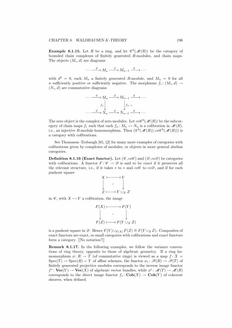
CHAPTER 8. WALDHAUSEN K-THEORY 196
Example 8.1.15. Let R be a ring, and let C b(M (R)) be the category ofbounded chain complexes of finitely generated R-modules, and chain maps.The objects (M∗, d) are diagrams
. . . d // Mnd // Mn−1
d // . . .
with d2 = 0, each Mn a finitely generated R-module, and Mn = 0 for alln sufficiently positive or sufficiently negative. The morphisms f∗ : (M∗, d) →(N∗, d) are commutative diagrams
. . . d // Mnd //
fn
²²
Mn−1d //
fn−1
²²
. . .
. . . d // Nnd // Nn−1
d // . . .
The zero object is the complex of zero modules. Let coC b(M (R)) be the subcat-egory of chain maps f∗ such that each fn : Mn Nn is a cofibration in M (R),i.e., an injective R-module homomorphism. Then (C b(M (R)), coC b(M (R))) isa category with cofibrations.
See Thomason–Trobaugh [65, §2] for many more examples of categories withcofibrations given by complexes of modules, or objects in more general abeliancategories.
Definition 8.1.16 (Exact functor). Let (C , coC ) and (D , coD) be categorieswith cofibrations. A functor F : C → D is said to be exact if it preserves allthe relevant structure, i.e., if it takes ∗ to ∗ and coC to coD , and if for eachpushout square
X // //
²²
p
Y
²²
Z // // Y ∪X Z
in C , with X Y a cofibration, the image
F (X) // //
²²
p
F (Y )
²²
F (Z) // // F (Y ∪X Z)
is a pushout square in D . Hence F (Y )∪F (X)F (Z) ∼= F (Y ∪X Z). Composites ofexact functors are exact, so small categories with cofibrations and exact functorsform a category. [[No notation?]]
Remark 8.1.17. In the following examples, we follow the variance conven-tions of ring theory, opposite to those of algebraic geometry. If a ring ho-momorphism φ : R → T (of commutative rings) is viewed as a map f : X =Spec(T ) → Spec(R) = Y of affine schemes, the functor φ∗ : P(R) → P(T ) offinitely generated projective modules corresponds to the inverse image functorf∗ : Vec(Y ) → Vec(X) of algebraic vector bundles, while φ∗ : M (T ) → M (R)corresponds to the direct image functor f∗ : Coh(X) → Coh(Y ) of coherentsheaves, when defined.
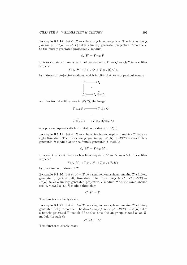
CHAPTER 8. WALDHAUSEN K-THEORY 197
Example 8.1.18. Let φ : R → T be a ring homomorphism. The inverse imagefunctor φ∗ : P(R) → P(T ) takes a finitely generated projective R-module Pto the finitely generated projective T -module
φ∗(P ) = T ⊗R P .
It is exact, since it maps each cofiber sequence P Q ։ Q/P to a cofibersequence
T ⊗R P T ⊗R Q ։ T ⊗R (Q/P ) ,
by flatness of projective modules, which implies that for any pushout square
P // //
²²
p
Q
²²
L // // Q ⊕P L
with horizontal cofibrations in P(R), the image
T ⊗R P // //
²²
p
T ⊗R Q
²²
T ⊗R L // // T ⊗R (Q ⊕P L)
is a pushout square with horizontal cofibrations in P(T ).
Example 8.1.19. Let φ : R → T be a ring homomorphism, making T flat as aright R-module. The inverse image functor φ∗ : M (R) → M (T ) takes a finitelygenerated R-module M to the finitely generated T -module
φ∗(M) = T ⊗R M .
It is exact, since it maps each cofiber sequence M N ։ N/M to a cofibersequence
T ⊗R M T ⊗R N ։ T ⊗R (N/M) ,
by the assumed flatness of T .
Example 8.1.20. Let φ : R → T be a ring homomorphism, making T a finitelygenerated projective (left) R-module. The direct image functor φ∗ : P(T ) →P(R) takes a finitely generated projective T -module P to the same abeliangroup, viewed as an R-module through φ:
φ∗(P ) = P .
This functor is clearly exact.
Example 8.1.21. Let φ : R → T be a ring homomorphism, making T a finitelygenerated (left) R-module. The direct image functor φ∗ : M (T ) → M (R) takesa finitely generated T -module M to the same abelian group, viewed as an R-module through φ:
φ∗(M) = M .
This functor is clearly exact.
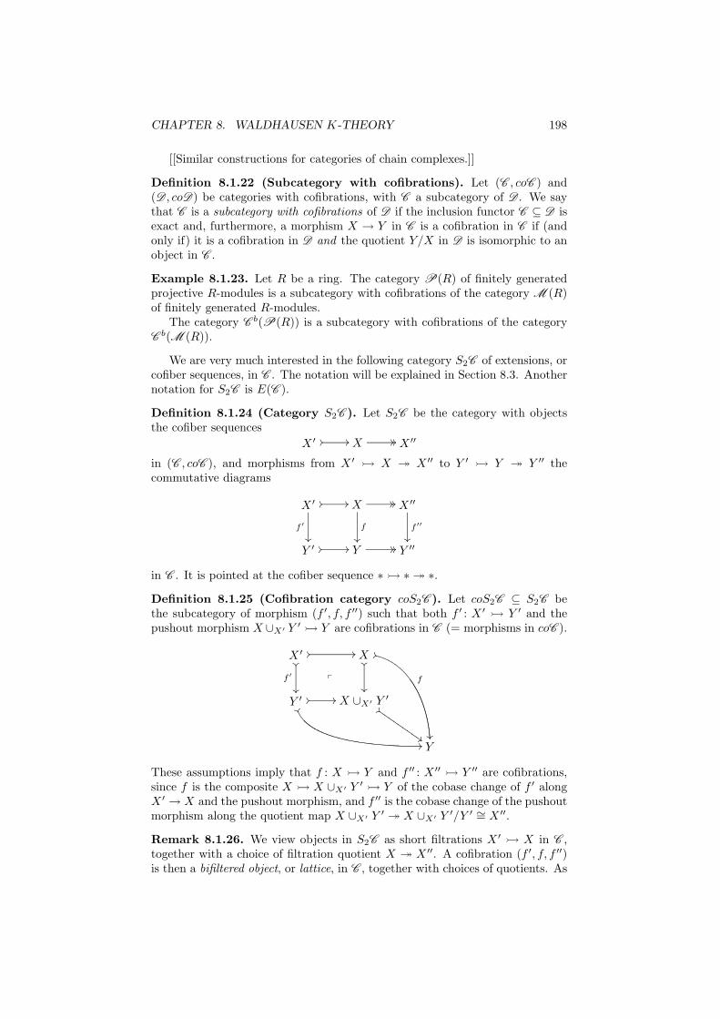
CHAPTER 8. WALDHAUSEN K-THEORY 198
[[Similar constructions for categories of chain complexes.]]
Definition 8.1.22 (Subcategory with cofibrations). Let (C , coC ) and(D , coD) be categories with cofibrations, with C a subcategory of D . We saythat C is a subcategory with cofibrations of D if the inclusion functor C ⊆ D isexact and, furthermore, a morphism X → Y in C is a cofibration in C if (andonly if) it is a cofibration in D and the quotient Y/X in D is isomorphic to anobject in C .
Example 8.1.23. Let R be a ring. The category P(R) of finitely generatedprojective R-modules is a subcategory with cofibrations of the category M (R)of finitely generated R-modules.
The category C b(P(R)) is a subcategory with cofibrations of the categoryC b(M (R)).
We are very much interested in the following category S2C of extensions, orcofiber sequences, in C . The notation will be explained in Section 8.3. Anothernotation for S2C is E(C ).
Definition 8.1.24 (Category S2C ). Let S2C be the category with objectsthe cofiber sequences
X ′ // // X // // X ′′
in (C , coC ), and morphisms from X ′ X ։ X ′′ to Y ′
Y ։ Y ′′ thecommutative diagrams
X ′
f ′
²²
// // X
f
²²
// // X ′′
f ′′
²²
Y ′ // // Y // // Y ′′
in C . It is pointed at the cofiber sequence ∗ ∗ ։ ∗.
Definition 8.1.25 (Cofibration category coS2C ). Let coS2C ⊆ S2C bethe subcategory of morphism (f ′, f, f ′′) such that both f ′ : X ′
Y ′ and thepushout morphism X ∪X′ Y ′
Y are cofibrations in C (= morphisms in coC ).
X ′ // //
²²
f ′
²²
p
X²²
²²
,,
f
³³
Y ′ // //
··
//
X ∪X′ Y ′
$$
$$IIIIIIIII
Y
These assumptions imply that f : X Y and f ′′ : X ′′ Y ′′ are cofibrations,
since f is the composite X X ∪X′ Y ′ Y of the cobase change of f ′ along
X ′ → X and the pushout morphism, and f ′′ is the cobase change of the pushoutmorphism along the quotient map X ∪X′ Y ′
։ X ∪X′ Y ′/Y ′ ∼= X ′′.
Remark 8.1.26. We view objects in S2C as short filtrations X ′ X in C ,
together with a choice of filtration quotient X ։ X ′′. A cofibration (f ′, f, f ′′)is then a bifiltered object, or lattice, in C , together with choices of quotients. As
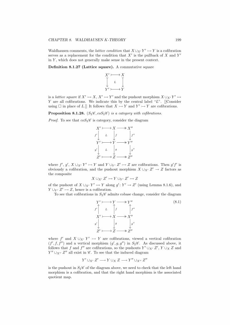
CHAPTER 8. WALDHAUSEN K-THEORY 199
Waldhausen comments, the lattice condition that X∪X′ Y ′ Y is a cofibration
serves as a replacement for the condition that X ′ is the pullback of X and Y ′
in Y , which does not generally make sense in the present context.
Definition 8.1.27 (Lattice square). A commutative square
X ′ // //
²²
²²
L
X²²
²²
Y ′ // // Y
is a lattice square if X ′ X, X ′
Y ′ and the pushout morphism X ∪X′ Y ′
Y are all cofibrations. We indicate this by the central label “L”. [[Considerusing ¤ in place of L.]] It follows that X Y and Y ′
Y are cofibrations.
Proposition 8.1.28. (S2C , coS2C ) is a category with cofibrations.
Proof. To see that coS2C is category, consider the diagram
X ′
f ′
²²
// //
L
X
f
²²
// // X ′′
f ′′
²²
Y ′
g′
²²
// //
L
Y
g
²²
// // Y ′′
g′′
²²
Z ′ // // Z // // Z ′′
where f ′, g′, X ∪X′ Y ′ Y and Y ∪Y ′ Z ′
Z are cofibrations. Then g′f ′ isobviously a cofibration, and the pushout morphism X ∪X′ Z ′ → Z factors asthe composite
X ∪X′ Z ′ Y ∪Y ′ Z ′
Z
of the pushout of X ∪X′ Y ′ Y along g′ : Y ′ → Z ′ (using Lemma 8.1.6), and
Y ∪Y ′ Z ′ Z, hence is a cofibration.
To see that cofibrations in S2C admits cobase change, consider the diagram
Y ′ // // Y // // Y ′′
X ′
f ′
OO
g′
²²
// //
L
X
f
OO
g
²²
// // X ′′
f ′′
OO
g′′
²²
Z ′ // // Z // // Z ′′
(8.1)
where f ′ and X ∪X′ Y ′ Y are cofibrations, viewed a vertical cofibration
(f ′, f, f ′′) and a vertical morphism (g′, g, g′′) in S2C . As discussed above, itfollows that f and f ′′ are cofibrations, so the pushouts Y ′ ∪X′ Z ′, Y ∪X Z andY ′′ ∪X′′ Z ′′ all exist in C . To see that the induced diagram
Y ′ ∪X′ Z ′ −→ Y ∪X Z −→ Y ′′ ∪X′′ Z ′′
is the pushout in S2C of the diagram above, we need to check that the left handmorphism is a cofibration, and that the right hand morphism is the associatedquotient map.
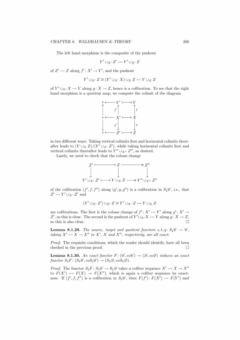
CHAPTER 8. WALDHAUSEN K-THEORY 200
The left hand morphism is the composite of the pushout
Y ′ ∪X′ Z ′ Y ′ ∪X′ Z
of Z ′ Z along f ′ : X ′ → Y ′, and the pushout
Y ′ ∪X′ Z ∼= (Y ′ ∪X′ X) ∪X Z Y ∪X Z
of Y ′ ∪X′ X Y along g : X → Z, hence is a cofibration. To see that the righthand morphism is a quotient map, we compute the colimit of the diagram
∗ Y ′ // //oo Y
∗
OO
²²
X ′ // //oo
f ′
OO
g′
²²
X
f
OO
g
²²
∗ Z ′ // //oo Z
in two different ways: Taking vertical colimits first and horizontal colimits there-after leads to (Y ∪X Z)/(Y ′ ∪X′ Z ′), while taking horizontal colimits first andvertical colimits thereafter leads to Y ′′ ∪X′′ Z ′′, as desired.
Lastly, we need to check that the cobase change
Z ′ // //
²²
Z // //
²²
Z ′′
²²
Y ′ ∪X′ Z ′ // // Y ∪X Z // // Y ′′ ∪X′′ Z ′′
of the cofibration (f ′, f, f ′′) along (g′, g, g′′) is a cofibration in S2C , i.e., thatZ ′
Y ′ ∪X′ Z ′ and
(Y ′ ∪X′ Z ′) ∪Z′ Z ∼= Y ′ ∪X′ Z Y ∪X Z
are cofibrations. The first is the cobase change of f ′ : X ′ Y ′ along g′ : X ′ →
Z ′, so this is clear. The second is the pushout of Y ′∪X′X Y along g : X → Z,so this is also clear.
Lemma 8.1.29. The source, target and quotient functors s, t, q : S2C → C ,taking X ′
X → X ′′ to X ′, X and X ′′, respectively, are all exact.
Proof. The requisite conditions, which the reader should identify, have all beenchecked in the previous proof.
Lemma 8.1.30. An exact functor F : (C , coC ) → (D , coD) induces an exactfunctor S2F : (S2C , coS2C ) → (S2D , coS2D).
Proof. The functor S2F : S2C → S2D takes a cofiber sequence X ′ X ։ X ′′
to F (X ′) F (X) ։ F (X ′′), which is again a cofiber sequence by exact-ness. If (f ′, f, f ′′) is a cofibration in S2C , then F (f ′) : F (X ′) F (Y ′) and
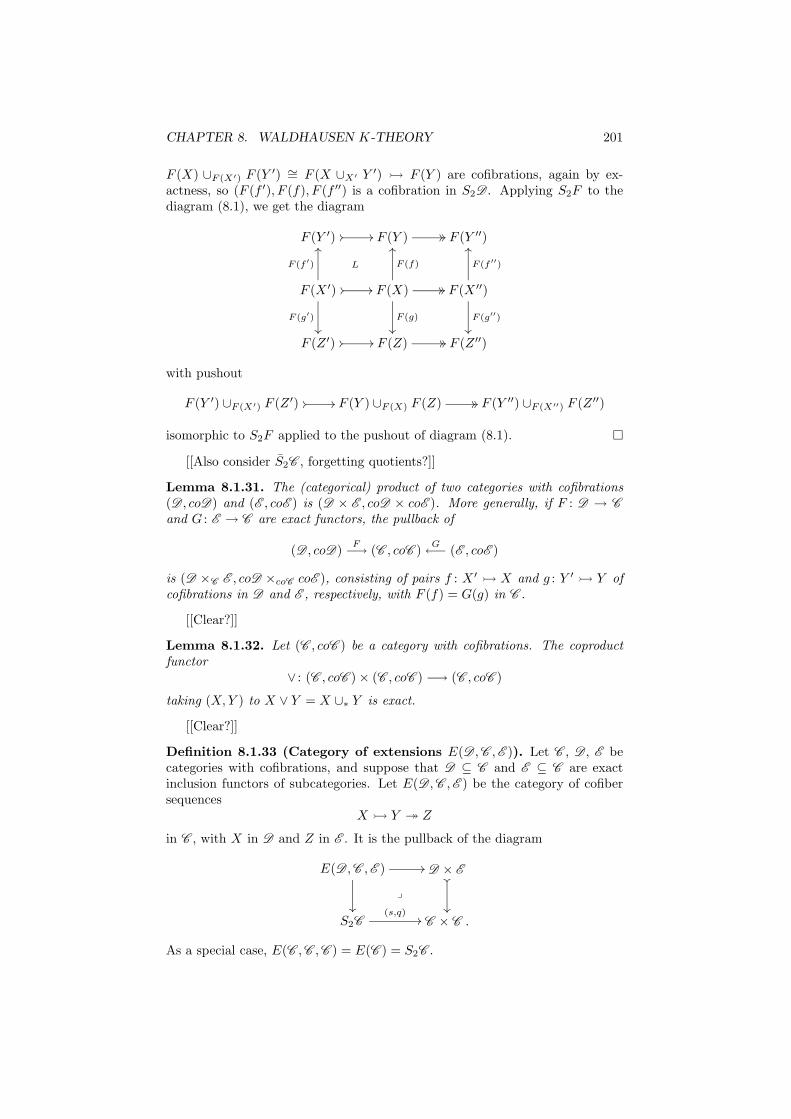
CHAPTER 8. WALDHAUSEN K-THEORY 201
F (X) ∪F (X′) F (Y ′) ∼= F (X ∪X′ Y ′) F (Y ) are cofibrations, again by ex-actness, so (F (f ′), F (f), F (f ′′) is a cofibration in S2D . Applying S2F to thediagram (8.1), we get the diagram
F (Y ′) // // F (Y ) // // F (Y ′′)
F (X ′)
F (f ′)
OO
F (g′)
²²
// //
L
F (X)
F (f)
OO
F (g)
²²
// // F (X ′′)
F (f ′′)
OO
F (g′′)
²²
F (Z ′) // // F (Z) // // F (Z ′′)
with pushout
F (Y ′) ∪F (X′) F (Z ′) // // F (Y ) ∪F (X) F (Z) // // F (Y ′′) ∪F (X′′) F (Z ′′)
isomorphic to S2F applied to the pushout of diagram (8.1).
[[Also consider S2C , forgetting quotients?]]
Lemma 8.1.31. The (categorical) product of two categories with cofibrations(D , coD) and (E , coE ) is (D × E , coD × coE ). More generally, if F : D → C
and G : E → C are exact functors, the pullback of
(D , coD)F−→ (C , coC )
G←− (E , coE )
is (D ×C E , coD ×coC coE ), consisting of pairs f : X ′ X and g : Y ′
Y ofcofibrations in D and E , respectively, with F (f) = G(g) in C .
[[Clear?]]
Lemma 8.1.32. Let (C , coC ) be a category with cofibrations. The coproductfunctor
∨ : (C , coC ) × (C , coC ) −→ (C , coC )
taking (X,Y ) to X ∨ Y = X ∪∗ Y is exact.
[[Clear?]]
Definition 8.1.33 (Category of extensions E(D ,C ,E )). Let C , D , E becategories with cofibrations, and suppose that D ⊆ C and E ⊆ C are exactinclusion functors of subcategories. Let E(D ,C ,E ) be the category of cofibersequences
X Y ։ Z
in C , with X in D and Z in E . It is the pullback of the diagram
E(D ,C ,E ) //
²²
y
D × E²²
²²
S2C(s,q)
// C × C .
As a special case, E(C ,C ,C ) = E(C ) = S2C .
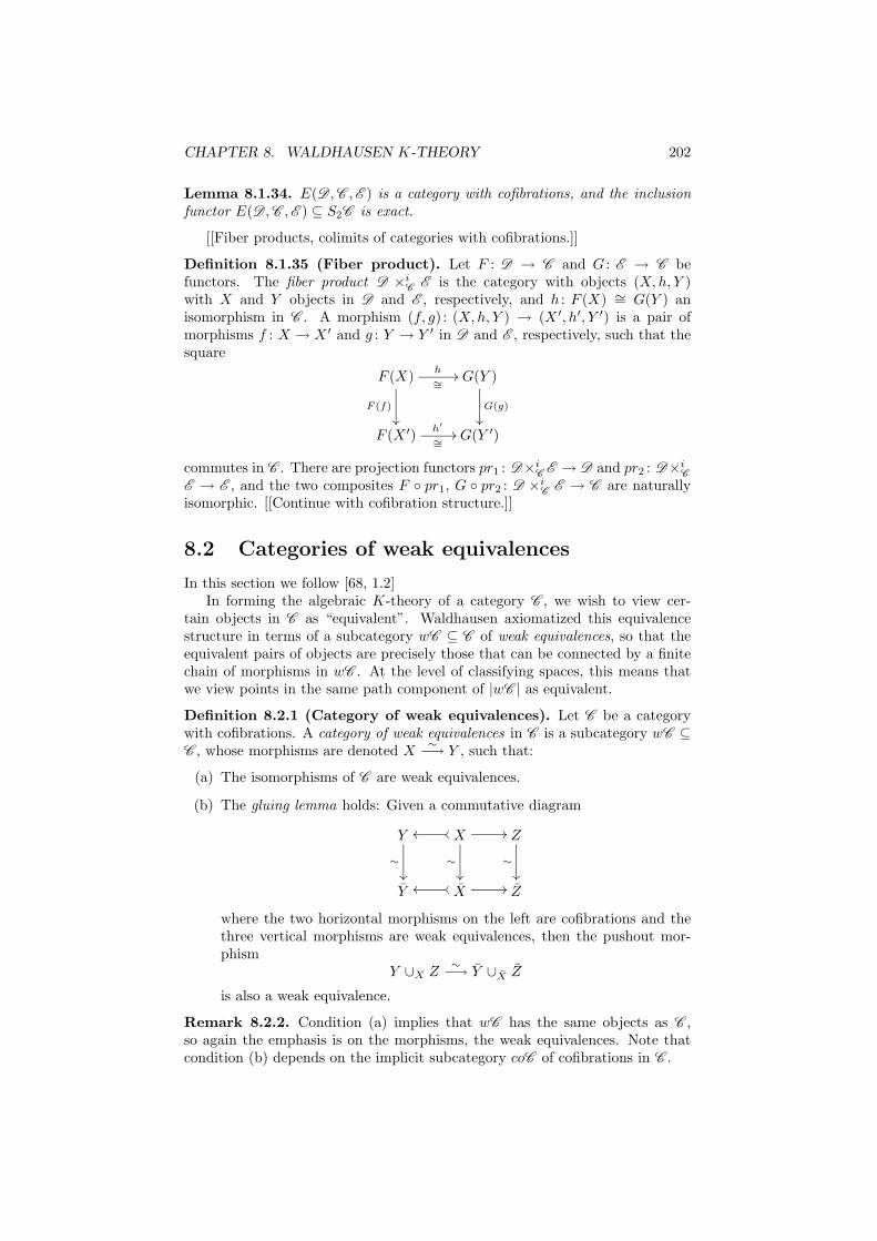
CHAPTER 8. WALDHAUSEN K-THEORY 202
Lemma 8.1.34. E(D ,C ,E ) is a category with cofibrations, and the inclusionfunctor E(D ,C ,E ) ⊆ S2C is exact.
[[Fiber products, colimits of categories with cofibrations.]]
Definition 8.1.35 (Fiber product). Let F : D → C and G : E → C befunctors. The fiber product D ×i
CE is the category with objects (X,h, Y )
with X and Y objects in D and E , respectively, and h : F (X) ∼= G(Y ) anisomorphism in C . A morphism (f, g) : (X,h, Y ) → (X ′, h′, Y ′) is a pair ofmorphisms f : X → X ′ and g : Y → Y ′ in D and E , respectively, such that thesquare
F (X)h∼=
//
F (f)
²²
G(Y )
G(g)
²²
F (X ′)h′
∼=// G(Y ′)
commutes in C . There are projection functors pr1 : D×iC
E → D and pr2 : D×iC
E → E , and the two composites F pr1, G pr2 : D ×iC
E → C are naturallyisomorphic. [[Continue with cofibration structure.]]
8.2 Categories of weak equivalences
In this section we follow [68, 1.2]In forming the algebraic K-theory of a category C , we wish to view cer-
tain objects in C as “equivalent”. Waldhausen axiomatized this equivalencestructure in terms of a subcategory wC ⊆ C of weak equivalences, so that theequivalent pairs of objects are precisely those that can be connected by a finitechain of morphisms in wC . At the level of classifying spaces, this means thatwe view points in the same path component of |wC | as equivalent.
Definition 8.2.1 (Category of weak equivalences). Let C be a categorywith cofibrations. A category of weak equivalences in C is a subcategory wC ⊆C , whose morphisms are denoted X
∼−→ Y , such that:
(a) The isomorphisms of C are weak equivalences.
(b) The gluing lemma holds: Given a commutative diagram
Y
∼
²²
Xoooo
∼
²²
// Z
∼
²²
Y Xoooo // Z
where the two horizontal morphisms on the left are cofibrations and thethree vertical morphisms are weak equivalences, then the pushout mor-phism
Y ∪X Z∼−→ Y ∪X Z
is also a weak equivalence.
Remark 8.2.2. Condition (a) implies that wC has the same objects as C ,so again the emphasis is on the morphisms, the weak equivalences. Note thatcondition (b) depends on the implicit subcategory coC of cofibrations in C .
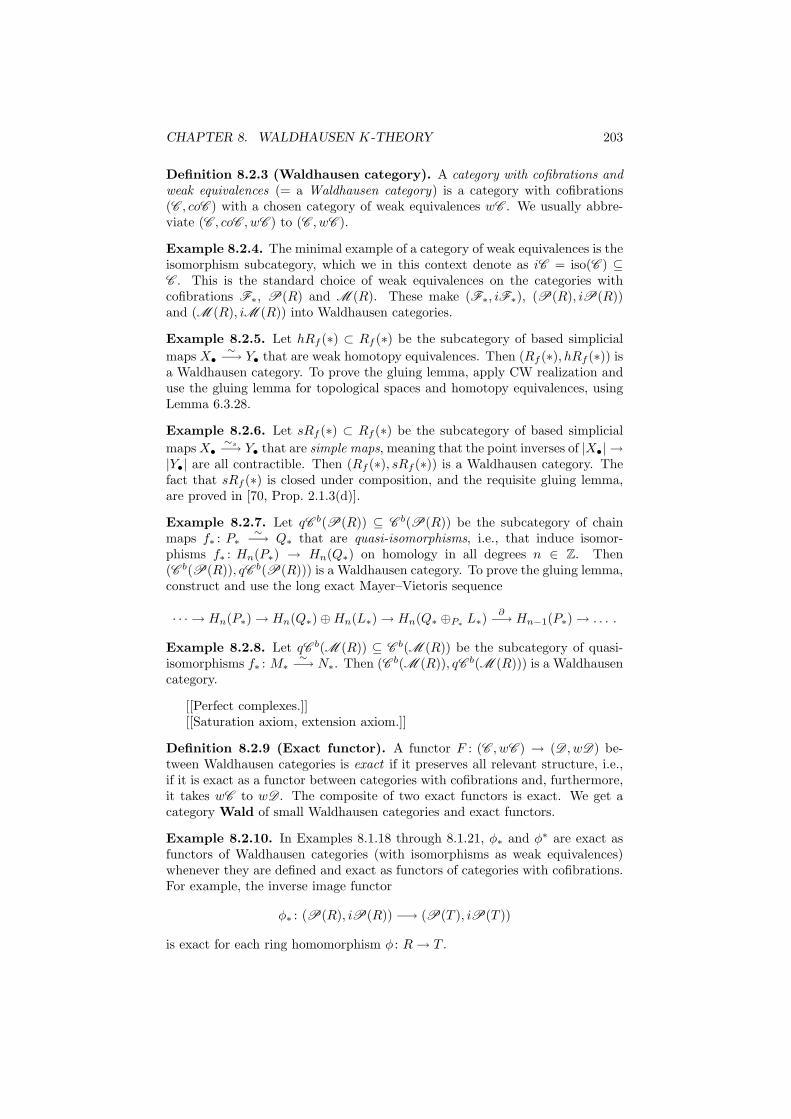
CHAPTER 8. WALDHAUSEN K-THEORY 203
Definition 8.2.3 (Waldhausen category). A category with cofibrations andweak equivalences (= a Waldhausen category) is a category with cofibrations(C , coC ) with a chosen category of weak equivalences wC . We usually abbre-viate (C , coC , wC ) to (C , wC ).
Example 8.2.4. The minimal example of a category of weak equivalences is theisomorphism subcategory, which we in this context denote as iC = iso(C ) ⊆C . This is the standard choice of weak equivalences on the categories withcofibrations F∗, P(R) and M (R). These make (F∗, iF∗), (P(R), iP(R))and (M (R), iM (R)) into Waldhausen categories.
Example 8.2.5. Let hRf (∗) ⊂ Rf (∗) be the subcategory of based simplicial
maps X•∼−→ Y• that are weak homotopy equivalences. Then (Rf (∗), hRf (∗)) is
a Waldhausen category. To prove the gluing lemma, apply CW realization anduse the gluing lemma for topological spaces and homotopy equivalences, usingLemma 6.3.28.
Example 8.2.6. Let sRf (∗) ⊂ Rf (∗) be the subcategory of based simplicial
maps X•∼s−→ Y• that are simple maps, meaning that the point inverses of |X•| →
|Y•| are all contractible. Then (Rf (∗), sRf (∗)) is a Waldhausen category. Thefact that sRf (∗) is closed under composition, and the requisite gluing lemma,are proved in [70, Prop. 2.1.3(d)].
Example 8.2.7. Let qC b(P(R)) ⊆ C b(P(R)) be the subcategory of chainmaps f∗ : P∗
∼−→ Q∗ that are quasi-isomorphisms, i.e., that induce isomor-
phisms f∗ : Hn(P∗) → Hn(Q∗) on homology in all degrees n ∈ Z. Then(C b(P(R)), qC b(P(R))) is a Waldhausen category. To prove the gluing lemma,construct and use the long exact Mayer–Vietoris sequence
· · · → Hn(P∗) → Hn(Q∗) ⊕ Hn(L∗) → Hn(Q∗ ⊕P∗L∗)
∂−→ Hn−1(P∗) → . . . .
Example 8.2.8. Let qC b(M (R)) ⊆ C b(M (R)) be the subcategory of quasi-isomorphisms f∗ : M∗
∼−→ N∗. Then (C b(M (R)), qC b(M (R))) is a Waldhausen
category.
[[Perfect complexes.]][[Saturation axiom, extension axiom.]]
Definition 8.2.9 (Exact functor). A functor F : (C , wC ) → (D , wD) be-tween Waldhausen categories is exact if it preserves all relevant structure, i.e.,if it is exact as a functor between categories with cofibrations and, furthermore,it takes wC to wD . The composite of two exact functors is exact. We get acategory Wald of small Waldhausen categories and exact functors.
Example 8.2.10. In Examples 8.1.18 through 8.1.21, φ∗ and φ∗ are exact asfunctors of Waldhausen categories (with isomorphisms as weak equivalences)whenever they are defined and exact as functors of categories with cofibrations.For example, the inverse image functor
φ∗ : (P(R), iP(R)) −→ (P(T ), iP(T ))
is exact for each ring homomorphism φ : R → T .
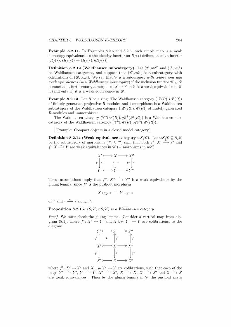
CHAPTER 8. WALDHAUSEN K-THEORY 204
Example 8.2.11. In Examples 8.2.5 and 8.2.6, each simple map is a weakhomotopy equivalence, so the identity functor on Rf (∗) defines an exact functor(Rf (∗), sRf (∗)) → (Rf (∗), hRf (∗)).
Definition 8.2.12 (Waldhausen subcategory). Let (C , wC ) and (D , wD)be Waldhausen categories, and suppose that (C , coC ) is a subcategory withcofibrations of (D , coD). We say that C is a subcategory with cofibrations andweak equivalences (= a Waldhausen subcategory) if the inclusion functor C ⊆ D
is exact and, furthermore, a morphism X → Y in C is a weak equivalence in C
if (and only if) it is a weak equivalence in D .
Example 8.2.13. Let R be a ring. The Waldhausen category (P(R), iP(R))of finitely generated projective R-modules and isomorphisms is a Waldhausensubcategory of the Waldhausen category (M (R), iM (R)) of finitely generatedR-modules and isomorphisms.
The Waldhausen category (C b(P(R)), qC b(P(R))) is a Waldhausen sub-category of the Waldhausen category (C b(M (R)), qC b(M (R))).
[[Example: Compact objects in a closed model category.]]
Definition 8.2.14 (Weak equivalence category wS2C ). Let wS2C ⊆ S2C
be the subcategory of morphisms (f ′, f, f ′′) such that both f ′ : X ′ ∼−→ Y ′ and
f : X∼−→ Y are weak equivalences in C (= morphisms in wC ).
X ′
f ′ ∼
²²
// // X
f ∼
²²
// // X ′′
f ′′ ∼
²²
Y ′ // // Y // // Y ′′
These assumptions imply that f ′′ : X ′′ ∼−→ Y ′′ is a weak equivalence by the
gluing lemma, since f ′′ is the pushout morphism
X ∪X′ ∗∼−→ Y ∪Y ′ ∗
of f and ∗∼−→ ∗ along f ′.
Proposition 8.2.15. (S2C , wS2C ) is a Waldhausen category.
Proof. We must check the gluing lemma. Consider a vertical map from dia-gram (8.1), where f ′ : X ′
Y ′ and X ∪X′ Y ′ Y are cofibrations, to the
diagram
Y ′ // // Y // // Y ′′
X ′
f ′
OO
g′
²²
// //
L
X
f
OO
g
²²
// // X ′′
f ′′
OO
g′′
²²
Z ′ // // Z // // Z ′′
where f ′ : X ′ Y ′ and X ∪X′ Y ′
Y are cofibrations, such that each of themaps Y ′ ∼
−→ Y ′, Y∼−→ Y , X ′ ∼
−→ X ′, X∼−→ X, Z ′ ∼
−→ Z ′ and Z∼−→ Z
are weak equivalences. Then by the gluing lemma in C the pushout maps
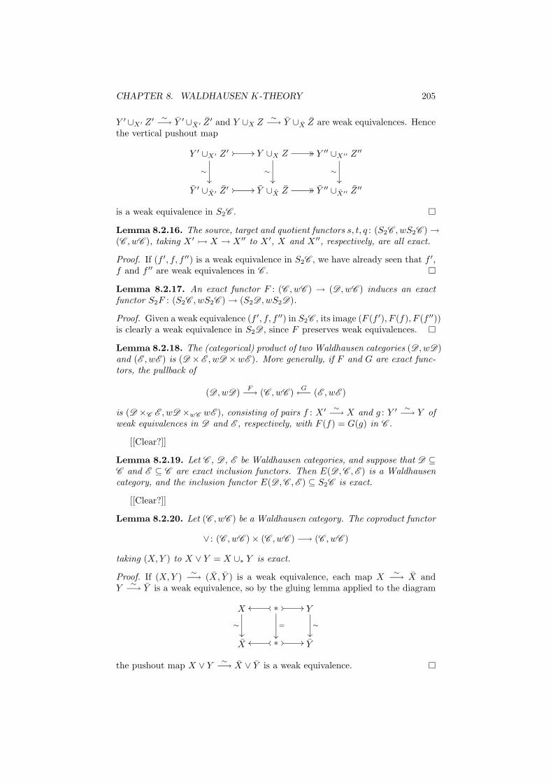
CHAPTER 8. WALDHAUSEN K-THEORY 205
Y ′ ∪X′ Z ′ ∼−→ Y ′ ∪X′ Z ′ and Y ∪X Z
∼−→ Y ∪X Z are weak equivalences. Hence
the vertical pushout map
Y ′ ∪X′ Z ′ // //
∼
²²
Y ∪X Z // //
∼
²²
Y ′′ ∪X′′ Z ′′
∼
²²
Y ′ ∪X′ Z ′ // // Y ∪X Z // // Y ′′ ∪X′′ Z ′′
is a weak equivalence in S2C .
Lemma 8.2.16. The source, target and quotient functors s, t, q : (S2C , wS2C ) →(C , wC ), taking X ′
X → X ′′ to X ′, X and X ′′, respectively, are all exact.
Proof. If (f ′, f, f ′′) is a weak equivalence in S2C , we have already seen that f ′,f and f ′′ are weak equivalences in C .
Lemma 8.2.17. An exact functor F : (C , wC ) → (D , wC ) induces an exactfunctor S2F : (S2C , wS2C ) → (S2D , wS2D).
Proof. Given a weak equivalence (f ′, f, f ′′) in S2C , its image (F (f ′), F (f), F (f ′′))is clearly a weak equivalence in S2D , since F preserves weak equivalences.
Lemma 8.2.18. The (categorical) product of two Waldhausen categories (D , wD)and (E , wE ) is (D × E , wD ×wE ). More generally, if F and G are exact func-tors, the pullback of
(D , wD)F−→ (C , wC )
G←− (E , wE )
is (D ×C E , wD ×wC wE ), consisting of pairs f : X ′ ∼−→ X and g : Y ′ ∼
−→ Y ofweak equivalences in D and E , respectively, with F (f) = G(g) in C .
[[Clear?]]
Lemma 8.2.19. Let C , D , E be Waldhausen categories, and suppose that D ⊆C and E ⊆ C are exact inclusion functors. Then E(D ,C ,E ) is a Waldhausencategory, and the inclusion functor E(D ,C ,E ) ⊆ S2C is exact.
[[Clear?]]
Lemma 8.2.20. Let (C , wC ) be a Waldhausen category. The coproduct functor
∨ : (C , wC ) × (C , wC ) −→ (C , wC )
taking (X,Y ) to X ∨ Y = X ∪∗ Y is exact.
Proof. If (X,Y )∼−→ (X, Y ) is a weak equivalence, each map X
∼−→ X and
Y∼−→ Y is a weak equivalence, so by the gluing lemma applied to the diagram
X
∼
²²
∗oooo // //
=
²²
Y
∼
²²
X ∗oooo // // Y
the pushout map X ∨ Y∼−→ X ∨ Y is a weak equivalence.
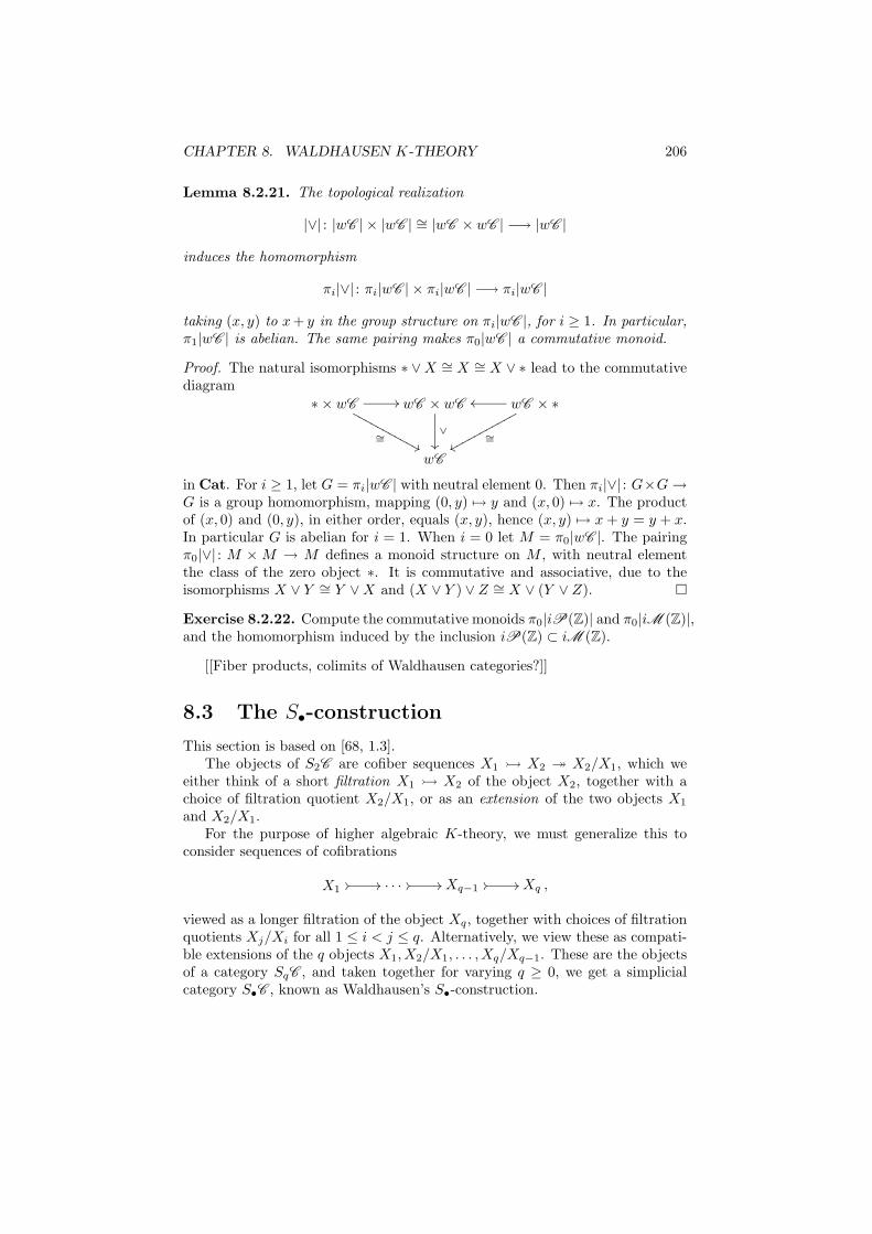
CHAPTER 8. WALDHAUSEN K-THEORY 206
Lemma 8.2.21. The topological realization
|∨| : |wC | × |wC | ∼= |wC × wC | −→ |wC |
induces the homomorphism
πi|∨| : πi|wC | × πi|wC | −→ πi|wC |
taking (x, y) to x + y in the group structure on πi|wC |, for i ≥ 1. In particular,π1|wC | is abelian. The same pairing makes π0|wC | a commutative monoid.
Proof. The natural isomorphisms ∗ ∨ X ∼= X ∼= X ∨ ∗ lead to the commutativediagram
∗ × wC //
∼=&&NNNNNNNNNNN wC × wC
∨
²²
wC × ∗oo
∼=xxqqqqqqqqqqq
wC
in Cat. For i ≥ 1, let G = πi|wC | with neutral element 0. Then πi|∨| : G×G →G is a group homomorphism, mapping (0, y) 7→ y and (x, 0) 7→ x. The productof (x, 0) and (0, y), in either order, equals (x, y), hence (x, y) 7→ x + y = y + x.In particular G is abelian for i = 1. When i = 0 let M = π0|wC |. The pairingπ0|∨| : M × M → M defines a monoid structure on M , with neutral elementthe class of the zero object ∗. It is commutative and associative, due to theisomorphisms X ∨ Y ∼= Y ∨ X and (X ∨ Y ) ∨ Z ∼= X ∨ (Y ∨ Z).
Exercise 8.2.22. Compute the commutative monoids π0|iP(Z)| and π0|iM (Z)|,and the homomorphism induced by the inclusion iP(Z) ⊂ iM (Z).
[[Fiber products, colimits of Waldhausen categories?]]
8.3 The S•-construction
This section is based on [68, 1.3].The objects of S2C are cofiber sequences X1 X2 ։ X2/X1, which we
either think of a short filtration X1 X2 of the object X2, together with achoice of filtration quotient X2/X1, or as an extension of the two objects X1
and X2/X1.For the purpose of higher algebraic K-theory, we must generalize this to
consider sequences of cofibrations
X1// // . . . // // Xq−1 // // Xq ,
viewed as a longer filtration of the object Xq, together with choices of filtrationquotients Xj/Xi for all 1 ≤ i < j ≤ q. Alternatively, we view these as compati-ble extensions of the q objects X1,X2/X1, . . . ,Xq/Xq−1. These are the objectsof a category SqC , and taken together for varying q ≥ 0, we get a simplicialcategory S•C , known as Waldhausen’s S•-construction.
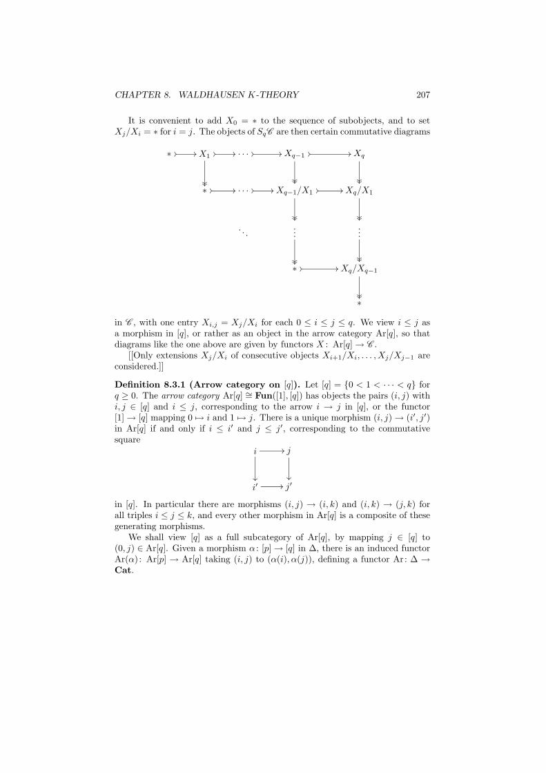
CHAPTER 8. WALDHAUSEN K-THEORY 207
It is convenient to add X0 = ∗ to the sequence of subobjects, and to setXj/Xi = ∗ for i = j. The objects of SqC are then certain commutative diagrams
∗ // // X1// //
²²²²
. . . // // Xq−1 // //
²²²²
Xq
²²²²
∗ // // . . . // // Xq−1/X1// //
²²²²
Xq/X1
²²²²
. . ....
²²²²
...
²²²²
∗ // // Xq/Xq−1
²²²²∗
in C , with one entry Xi,j = Xj/Xi for each 0 ≤ i ≤ j ≤ q. We view i ≤ j asa morphism in [q], or rather as an object in the arrow category Ar[q], so thatdiagrams like the one above are given by functors X : Ar[q] → C .
[[Only extensions Xj/Xi of consecutive objects Xi+1/Xi, . . . ,Xj/Xj−1 areconsidered.]]
Definition 8.3.1 (Arrow category on [q]). Let [q] = 0 < 1 < · · · < q forq ≥ 0. The arrow category Ar[q] ∼= Fun([1], [q]) has objects the pairs (i, j) withi, j ∈ [q] and i ≤ j, corresponding to the arrow i → j in [q], or the functor[1] → [q] mapping 0 7→ i and 1 7→ j. There is a unique morphism (i, j) → (i′, j′)in Ar[q] if and only if i ≤ i′ and j ≤ j′, corresponding to the commutativesquare
i //
²²
j
²²
i′ // j′
in [q]. In particular there are morphisms (i, j) → (i, k) and (i, k) → (j, k) forall triples i ≤ j ≤ k, and every other morphism in Ar[q] is a composite of thesegenerating morphisms.
We shall view [q] as a full subcategory of Ar[q], by mapping j ∈ [q] to(0, j) ∈ Ar[q]. Given a morphism α : [p] → [q] in ∆, there is an induced functorAr(α) : Ar[p] → Ar[q] taking (i, j) to (α(i), α(j)), defining a functor Ar: ∆ →Cat.
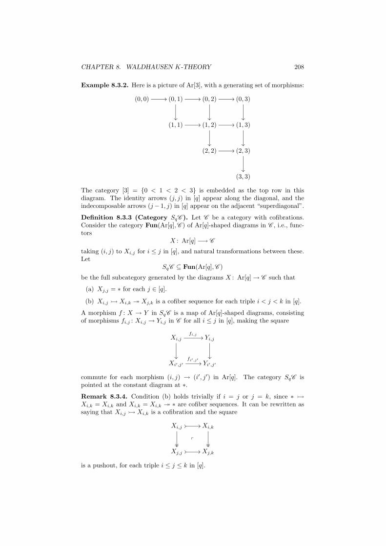
CHAPTER 8. WALDHAUSEN K-THEORY 208
Example 8.3.2. Here is a picture of Ar[3], with a generating set of morphisms:
(0, 0) // (0, 1) //
²²
(0, 2) //
²²
(0, 3)
²²
(1, 1) // (1, 2) //
²²
(1, 3)
²²
(2, 2) // (2, 3)
²²
(3, 3)
The category [3] = 0 < 1 < 2 < 3 is embedded as the top row in thisdiagram. The identity arrows (j, j) in [q] appear along the diagonal, and theindecomposable arrows (j − 1, j) in [q] appear on the adjacent “superdiagonal”.
Definition 8.3.3 (Category SqC ). Let C be a category with cofibrations.Consider the category Fun(Ar[q],C ) of Ar[q]-shaped diagrams in C , i.e., func-tors
X : Ar[q] −→ C
taking (i, j) to Xi,j for i ≤ j in [q], and natural transformations between these.Let
SqC ⊆ Fun(Ar[q],C )
be the full subcategory generated by the diagrams X : Ar[q] → C such that
(a) Xj,j = ∗ for each j ∈ [q].
(b) Xi,j Xi,k ։ Xj,k is a cofiber sequence for each triple i < j < k in [q].
A morphism f : X → Y in SqC is a map of Ar[q]-shaped diagrams, consistingof morphisms fi,j : Xi,j → Yi,j in C for all i ≤ j in [q], making the square
Xi,jfi,j
//
²²
Yi,j
²²
Xi′,j′
fi′,j′// Yi′,j′
commute for each morphism (i, j) → (i′, j′) in Ar[q]. The category SqC ispointed at the constant diagram at ∗.
Remark 8.3.4. Condition (b) holds trivially if i = j or j = k, since ∗
Xi,k = Xi,k and Xi,k = Xi,k ։ ∗ are cofiber sequences. It can be rewritten assaying that Xi,j Xi,k is a cofibration and the square
Xi,j // //
²²²²
p
Xi,k
²²²²
Xj,j // // Xj,k
is a pushout, for each triple i ≤ j ≤ k in [q].
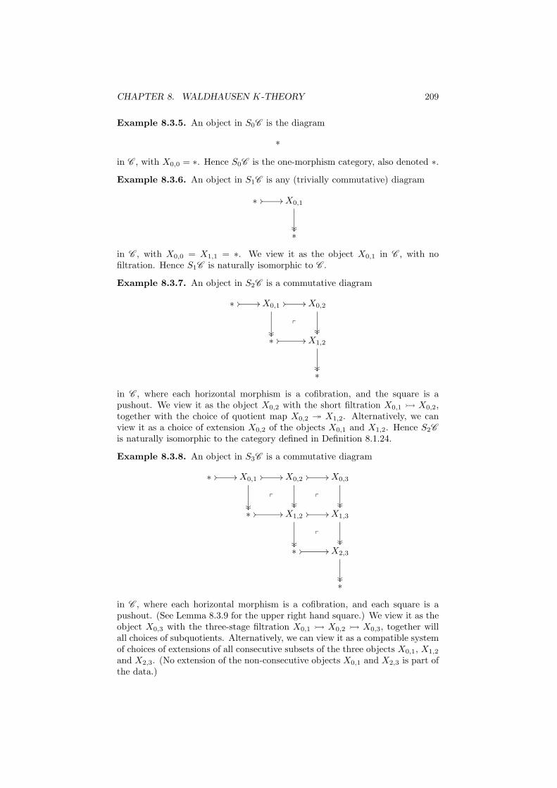
CHAPTER 8. WALDHAUSEN K-THEORY 209
Example 8.3.5. An object in S0C is the diagram
∗
in C , with X0,0 = ∗. Hence S0C is the one-morphism category, also denoted ∗.
Example 8.3.6. An object in S1C is any (trivially commutative) diagram
∗ // // X0,1
²²²²∗
in C , with X0,0 = X1,1 = ∗. We view it as the object X0,1 in C , with nofiltration. Hence S1C is naturally isomorphic to C .
Example 8.3.7. An object in S2C is a commutative diagram
∗ // // X0,1 // //
²²²²
p
X0,2
²²²²
∗ // // X1,2
²²²²∗
in C , where each horizontal morphism is a cofibration, and the square is apushout. We view it as the object X0,2 with the short filtration X0,1 X0,2,together with the choice of quotient map X0,2 ։ X1,2. Alternatively, we canview it as a choice of extension X0,2 of the objects X0,1 and X1,2. Hence S2C
is naturally isomorphic to the category defined in Definition 8.1.24.
Example 8.3.8. An object in S3C is a commutative diagram
∗ // // X0,1 // //
²²²²
p
X0,2 // //
²²²²
p
X0,3
²²²²
∗ // // X1,2 // //
²²²²
p
X1,3
²²²²
∗ // // X2,3
²²²²∗
in C , where each horizontal morphism is a cofibration, and each square is apushout. (See Lemma 8.3.9 for the upper right hand square.) We view it as theobject X0,3 with the three-stage filtration X0,1 X0,2 X0,3, together willall choices of subquotients. Alternatively, we can view it as a compatible systemof choices of extensions of all consecutive subsets of the three objects X0,1, X1,2
and X2,3. (No extension of the non-consecutive objects X0,1 and X2,3 is part ofthe data.)
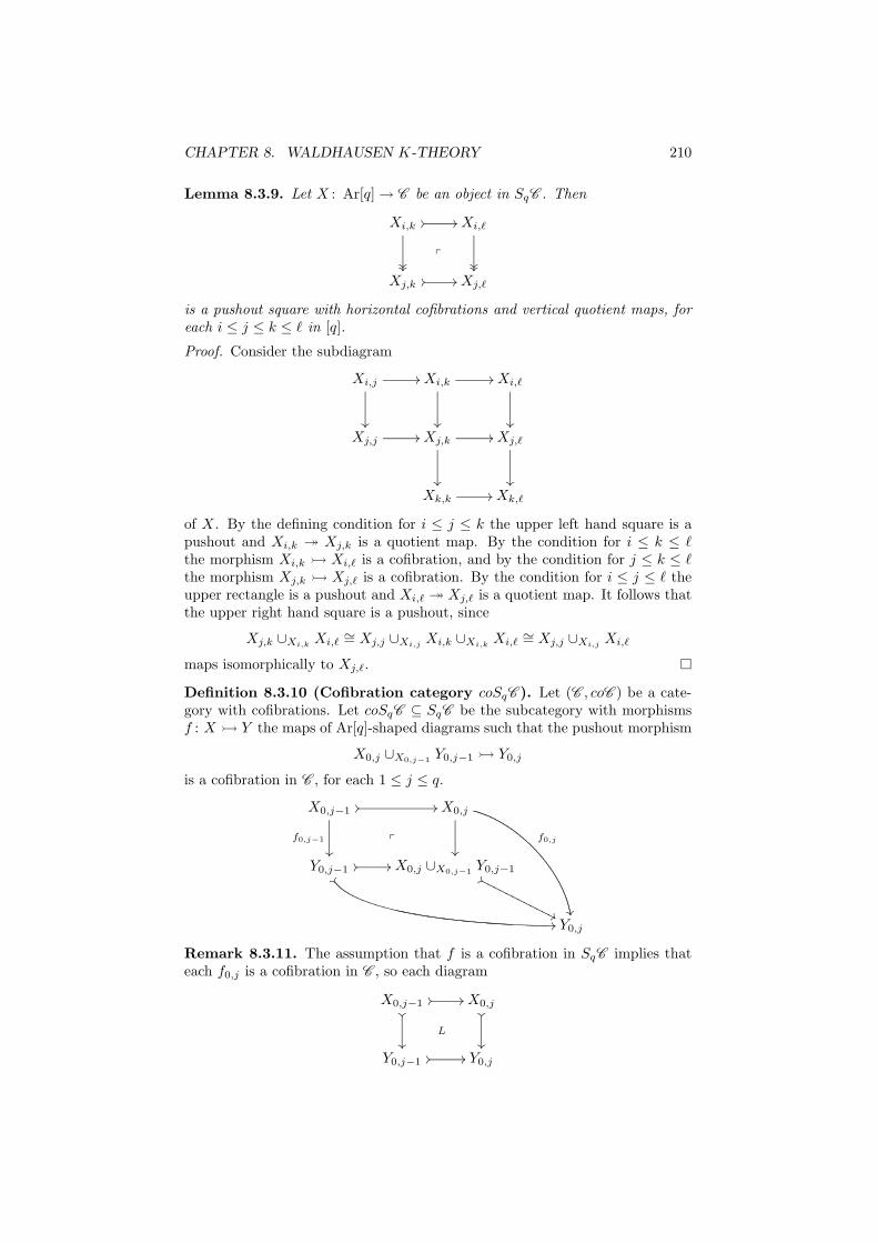
CHAPTER 8. WALDHAUSEN K-THEORY 210
Lemma 8.3.9. Let X : Ar[q] → C be an object in SqC . Then
Xi,k // //
²²²²
p
Xi,ℓ
²²²²
Xj,k // // Xj,ℓ
is a pushout square with horizontal cofibrations and vertical quotient maps, foreach i ≤ j ≤ k ≤ ℓ in [q].
Proof. Consider the subdiagram
Xi,j //
²²
Xi,k //
²²
Xi,ℓ
²²
Xj,j // Xj,k //
²²
Xj,ℓ
²²
Xk,k // Xk,ℓ
of X. By the defining condition for i ≤ j ≤ k the upper left hand square is apushout and Xi,k ։ Xj,k is a quotient map. By the condition for i ≤ k ≤ ℓthe morphism Xi,k Xi,ℓ is a cofibration, and by the condition for j ≤ k ≤ ℓthe morphism Xj,k Xj,ℓ is a cofibration. By the condition for i ≤ j ≤ ℓ theupper rectangle is a pushout and Xi,ℓ ։ Xj,ℓ is a quotient map. It follows thatthe upper right hand square is a pushout, since
Xj,k ∪Xi,kXi,ℓ
∼= Xj,j ∪Xi,jXi,k ∪Xi,k
Xi,ℓ∼= Xj,j ∪Xi,j
Xi,ℓ
maps isomorphically to Xj,ℓ.
Definition 8.3.10 (Cofibration category coSqC ). Let (C , coC ) be a cate-gory with cofibrations. Let coSqC ⊆ SqC be the subcategory with morphismsf : X Y the maps of Ar[q]-shaped diagrams such that the pushout morphism
X0,j ∪X0,j−1Y0,j−1 Y0,j
is a cofibration in C , for each 1 ≤ j ≤ q.
X0,j−1 // //
f0,j−1
²²
p
X0,j
²²
f0,j
µµ
Y0,j−1 // //
¼¼
//
X0,j ∪X0,j−1Y0,j−1''
''OOOOOOOOOOOO
Y0,j
Remark 8.3.11. The assumption that f is a cofibration in SqC implies thateach f0,j is a cofibration in C , so each diagram
X0,j−1 // //
²²
²²
L
X0,j²²
²²
Y0,j−1 // // Y0,j
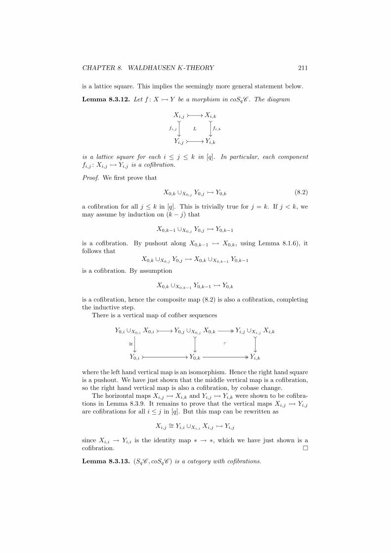
CHAPTER 8. WALDHAUSEN K-THEORY 211
is a lattice square. This implies the seemingly more general statement below.
Lemma 8.3.12. Let f : X Y be a morphism in coSqC . The diagram
Xi,j // //
²²
fi,j
²²
L
Xi,k²²
fi,k
²²
Yi,j // // Yi,k
is a lattice square for each i ≤ j ≤ k in [q]. In particular, each componentfi,j : Xi,j Yi,j is a cofibration.
Proof. We first prove that
X0,k ∪X0,jY0,j Y0,k (8.2)
a cofibration for all j ≤ k in [q]. This is trivially true for j = k. If j < k, wemay assume by induction on (k − j) that
X0,k−1 ∪X0,jY0,j Y0,k−1
is a cofibration. By pushout along X0,k−1 X0,k, using Lemma 8.1.6), itfollows that
X0,k ∪X0,jY0,j X0,k ∪X0,k−1
Y0,k−1
is a cofibration. By assumption
X0,k ∪X0,k−1Y0,k−1 Y0,k
is a cofibration, hence the composite map (8.2) is also a cofibration, completingthe inductive step.
There is a vertical map of cofiber sequences
Y0,i ∪X0,iX0,i // //
∼=
²²
Y0,j ∪X0,jX0,k // //
²²
²²
p
Yi,j ∪Xi,jXi,k
²²
²²
Y0,i // // Y0,k // // Yi,k
where the left hand vertical map is an isomorphism. Hence the right hand squareis a pushout. We have just shown that the middle vertical map is a cofibration,so the right hand vertical map is also a cofibration, by cobase change.
The horizontal maps Xi,j Xi,k and Yi,j Yi,k were shown to be cofibra-tions in Lemma 8.3.9. It remains to prove that the vertical maps Xi,j Yi,j
are cofibrations for all i ≤ j in [q]. But this map can be rewritten as
Xi,j∼= Yi,i ∪Xi,i
Xi,j Yi,j
since Xi,i → Yi,i is the identity map ∗ → ∗, which we have just shown is acofibration.
Lemma 8.3.13. (SqC , coSqC ) is a category with cofibrations.
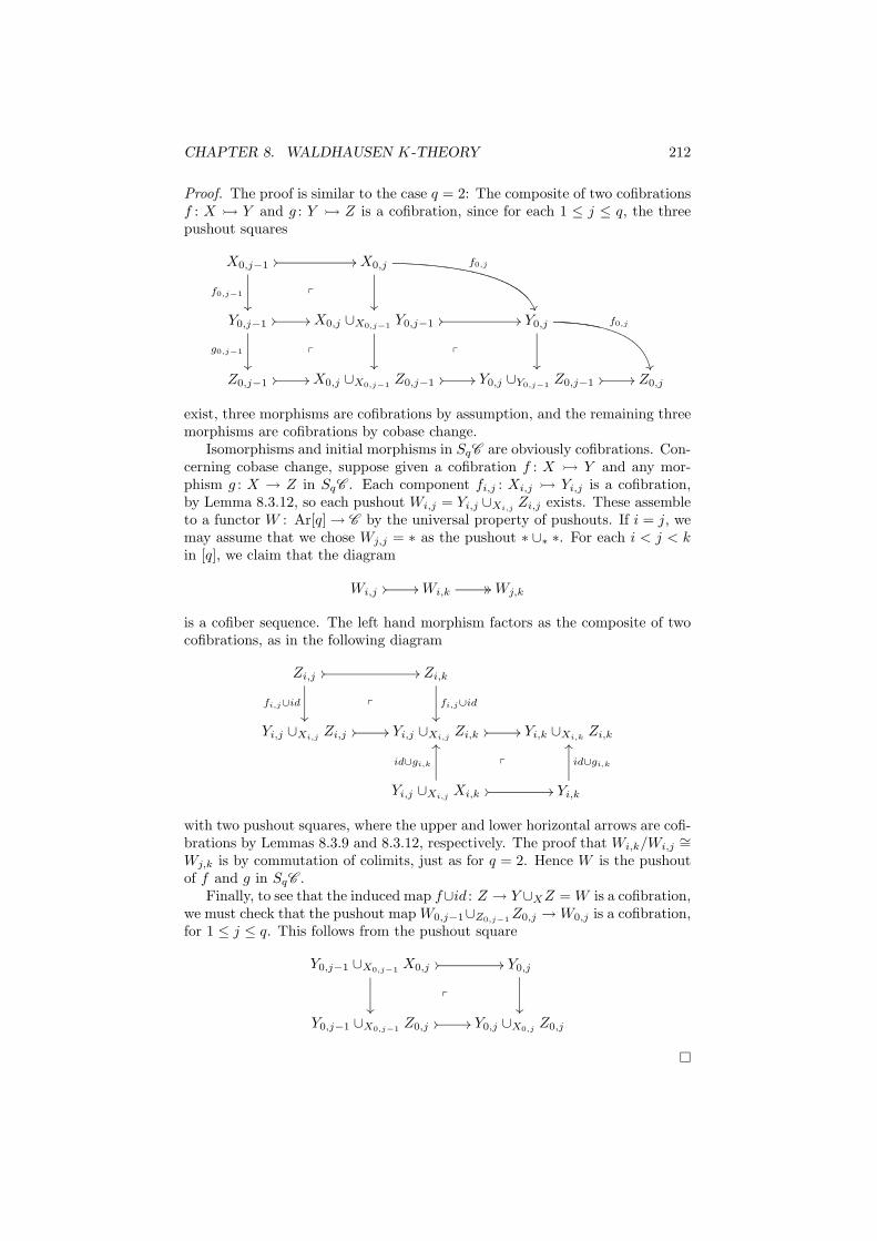
CHAPTER 8. WALDHAUSEN K-THEORY 212
Proof. The proof is similar to the case q = 2: The composite of two cofibrationsf : X Y and g : Y Z is a cofibration, since for each 1 ≤ j ≤ q, the threepushout squares
X0,j−1 // //
f0,j−1
²²
p
X0,j
²²
f0,j
¸¸
Y0,j−1 // //
g0,j−1
²²
p
X0,j ∪X0,j−1Y0,j−1
²²
// //
p
Y0,j
²²
f0,j
µµ
Z0,j−1 // // X0,j ∪X0,j−1Z0,j−1 // // Y0,j ∪Y0,j−1
Z0,j−1 // // Z0,j
exist, three morphisms are cofibrations by assumption, and the remaining threemorphisms are cofibrations by cobase change.
Isomorphisms and initial morphisms in SqC are obviously cofibrations. Con-cerning cobase change, suppose given a cofibration f : X Y and any mor-phism g : X → Z in SqC . Each component fi,j : Xi,j Yi,j is a cofibration,by Lemma 8.3.12, so each pushout Wi,j = Yi,j ∪Xi,j
Zi,j exists. These assembleto a functor W : Ar[q] → C by the universal property of pushouts. If i = j, wemay assume that we chose Wj,j = ∗ as the pushout ∗ ∪∗ ∗. For each i < j < kin [q], we claim that the diagram
Wi,j // // Wi,k // // Wj,k
is a cofiber sequence. The left hand morphism factors as the composite of twocofibrations, as in the following diagram
Zi,j
fi,j∪id
²²
// //
p
Zi,k
fi,j∪id
²²
Yi,j ∪Xi,jZi,j // // Yi,j ∪Xi,j
Zi,k // //
p
Yi,k ∪Xi,kZi,k
Yi,j ∪Xi,jXi,k
id∪gi,k
OO
// // Yi,k
id∪gi,k
OO
with two pushout squares, where the upper and lower horizontal arrows are cofi-brations by Lemmas 8.3.9 and 8.3.12, respectively. The proof that Wi,k/Wi,j
∼=Wj,k is by commutation of colimits, just as for q = 2. Hence W is the pushoutof f and g in SqC .
Finally, to see that the induced map f∪id : Z → Y ∪XZ = W is a cofibration,we must check that the pushout map W0,j−1∪Z0,j−1
Z0,j → W0,j is a cofibration,for 1 ≤ j ≤ q. This follows from the pushout square
Y0,j−1 ∪X0,j−1X0,j // //
²²
p
Y0,j
²²
Y0,j−1 ∪X0,j−1Z0,j // // Y0,j ∪X0,j
Z0,j
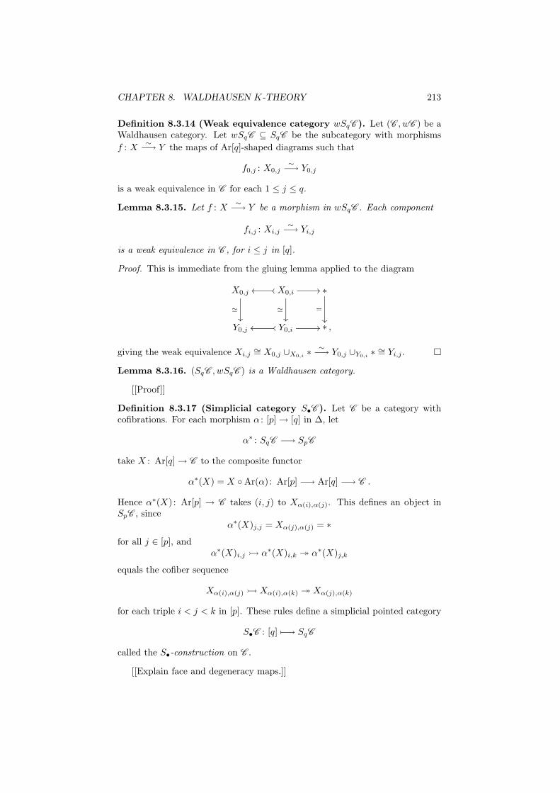
CHAPTER 8. WALDHAUSEN K-THEORY 213
Definition 8.3.14 (Weak equivalence category wSqC ). Let (C , wC ) be aWaldhausen category. Let wSqC ⊆ SqC be the subcategory with morphisms
f : X∼−→ Y the maps of Ar[q]-shaped diagrams such that
f0,j : X0,j∼−→ Y0,j
is a weak equivalence in C for each 1 ≤ j ≤ q.
Lemma 8.3.15. Let f : X∼−→ Y be a morphism in wSqC . Each component
fi,j : Xi,j∼−→ Yi,j
is a weak equivalence in C , for i ≤ j in [q].
Proof. This is immediate from the gluing lemma applied to the diagram
X0,j
≃
²²
X0,ioooo //
≃
²²
∗
=
²²Y0,j Y0,ioooo // ∗ ,
giving the weak equivalence Xi,j∼= X0,j ∪X0,i
∗∼−→ Y0,j ∪Y0,i
∗ ∼= Yi,j .
Lemma 8.3.16. (SqC , wSqC ) is a Waldhausen category.
[[Proof]]
Definition 8.3.17 (Simplicial category S•C ). Let C be a category withcofibrations. For each morphism α : [p] → [q] in ∆, let
α∗ : SqC −→ SpC
take X : Ar[q] → C to the composite functor
α∗(X) = X Ar(α) : Ar[p] −→ Ar[q] −→ C .
Hence α∗(X) : Ar[p] → C takes (i, j) to Xα(i),α(j). This defines an object inSpC , since
α∗(X)j,j = Xα(j),α(j) = ∗
for all j ∈ [p], andα∗(X)i,j α∗(X)i,k ։ α∗(X)j,k
equals the cofiber sequence
Xα(i),α(j) Xα(i),α(k) ։ Xα(j),α(k)
for each triple i < j < k in [p]. These rules define a simplicial pointed category
S•C : [q] 7−→ SqC
called the S•-construction on C .
[[Explain face and degeneracy maps.]]
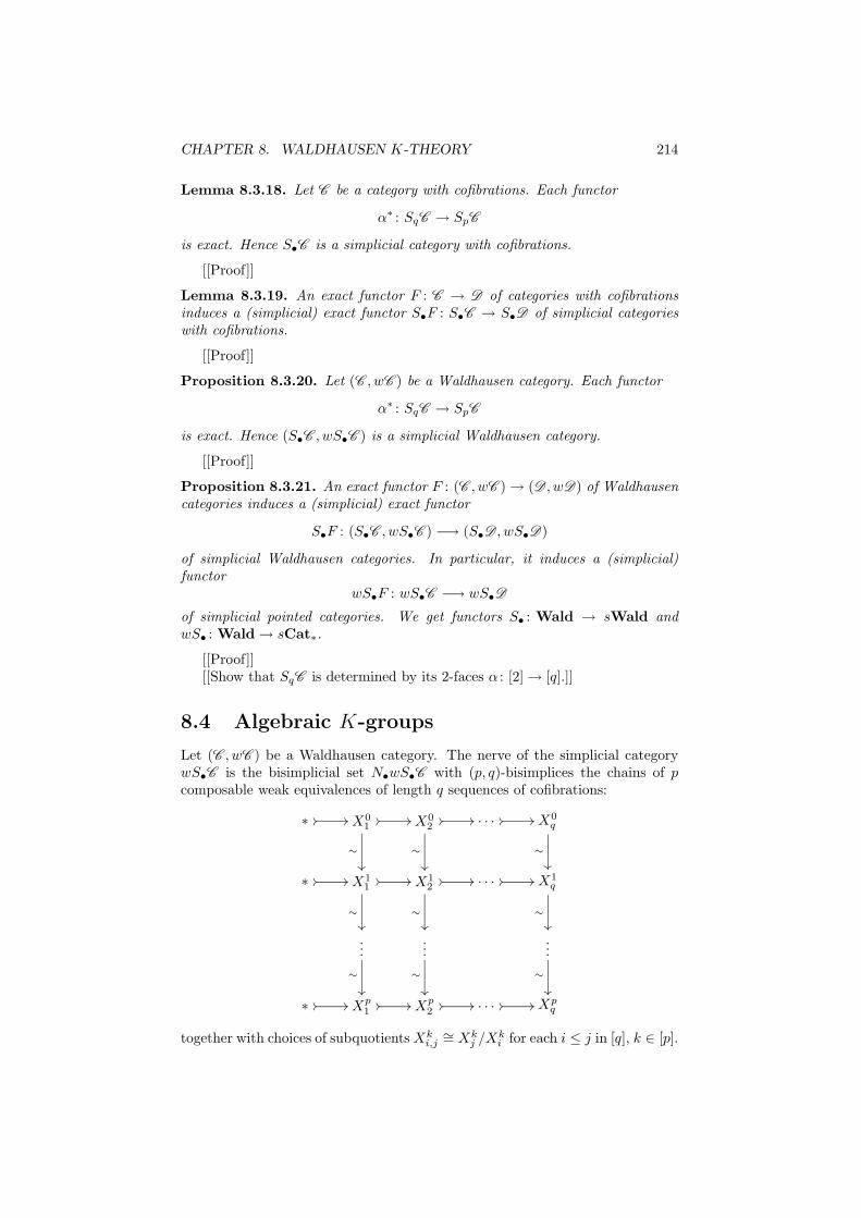
CHAPTER 8. WALDHAUSEN K-THEORY 214
Lemma 8.3.18. Let C be a category with cofibrations. Each functor
α∗ : SqC → SpC
is exact. Hence S•C is a simplicial category with cofibrations.
[[Proof]]
Lemma 8.3.19. An exact functor F : C → D of categories with cofibrationsinduces a (simplicial) exact functor S•F : S•C → S•D of simplicial categorieswith cofibrations.
[[Proof]]
Proposition 8.3.20. Let (C , wC ) be a Waldhausen category. Each functor
α∗ : SqC → SpC
is exact. Hence (S•C , wS•C ) is a simplicial Waldhausen category.
[[Proof]]
Proposition 8.3.21. An exact functor F : (C , wC ) → (D , wD) of Waldhausencategories induces a (simplicial) exact functor
S•F : (S•C , wS•C ) −→ (S•D , wS•D)
of simplicial Waldhausen categories. In particular, it induces a (simplicial)functor
wS•F : wS•C −→ wS•D
of simplicial pointed categories. We get functors S• : Wald → sWald andwS• : Wald → sCat∗.
[[Proof]][[Show that SqC is determined by its 2-faces α : [2] → [q].]]
8.4 Algebraic K-groups
Let (C , wC ) be a Waldhausen category. The nerve of the simplicial categorywS•C is the bisimplicial set N•wS•C with (p, q)-bisimplices the chains of pcomposable weak equivalences of length q sequences of cofibrations:
∗ // // X01
// //
∼
²²
X02
// //
∼
²²
. . . // // X0q
∼
²²
∗ // // X11
// //
∼
²²
X12
// //
∼
²²
. . . // // X1q
∼
²²
...
∼
²²
...
∼
²²
...
∼
²²
∗ // // Xp1
// // Xp2
// // . . . // // Xpq
together with choices of subquotients Xki,j
∼= Xkj /Xk
i for each i ≤ j in [q], k ∈ [p].
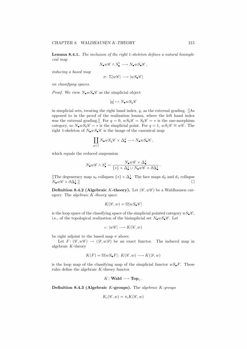
CHAPTER 8. WALDHAUSEN K-THEORY 215
Lemma 8.4.1. The inclusion of the right 1-skeleton defines a natural bisimpli-cial map
N•wC ∧ S1• −→ N•wS•C ,
inducing a based mapσ : Σ|wC | −→ |wS•C |
on classifying spaces.
Proof. We view N•wS•C as the simplicial object
[q] 7→ N•wSqC
in simplicial sets, treating the right hand index, q, as the external grading. [[Asopposed to in the proof of the realization lemma, where the left hand indexwas the external grading.]] For q = 0, wS0C = S0C = ∗ is the one-morphismcategory, so N•wS0C = ∗ is the simplicial point. For q = 1, wS1C
∼= wC . Theright 1-skeleton of N•wS•C is the image of the canonical map
∐
q≤1
N•wSqC × ∆q• −→ N•wS•C ,
which equals the reduced suspension
N•wC ∧ S1• =
N•wC × ∆1•
∗ × ∆1• ∪ N•wC × ∂∆1
•
.
[[The degeneracy map s0 collapses ∗ ×∆1•. The face maps d0 and d1 collapse
N•wC × ∂∆1•.]]
Definition 8.4.2 (Algebraic K-theory). Let (C , wC ) be a Waldhausen cat-egory. The algebraic K-theory space
K(C , w) = Ω|wS•C |
is the loop space of the classifying space of the simplicial pointed category wS•C ,i.e., of the topological realization of the bisimplicial set N•wS•C . Let
ι : |wC | −→ K(C , w)
be right adjoint to the based map σ above.Let F : (C , wC ) → (D , wD) be an exact functor. The induced map in
algebraic K-theory
K(F ) = Ω|wS•F | : K(C , w) −→ K(D , w)
is the loop map of the classifying map of the simplicial functor wS•F . Theserules define the algebraic K-theory functor
K : Wald −→ Top∗ .
Definition 8.4.3 (Algebraic K-groups). The algebraic K-groups
Ki(C , w) = πiK(C , w)
CHAPTER 8. WALDHAUSEN K-THEORY 216
of a Waldhausen category (C , wC ) are the homotopy groups, for i ≥ 0, of thealgebraic K-theory space. The induced homomorphism
Ki(F ) : Ki(C , w) −→ Ki(D , w)
of an exact functor F : (C , wC ) → (D , wD), is the homomorphism Ki(F ) =πiK(F ) induced by the based map of algebraic K-theory spaces. These rulesdefine the algebraic K-group functors
Ki : Wald → Ab .
Remark 8.4.4. The space |wS•C | is connected, since wS0C = ∗ in simplicialdegree 0 and all higher simplices are attached to this point. Hence no homo-topical information is lost by passing to the loop space Ω|wS•C |.
Remark 8.4.5. It is clear that Ki(C , w) = πi+1|wS•C | is abelian for i ≥ 1.The assertion that K0(C , w) is abelian follows from the next lemma, since the(split) cofiber sequences X ′
X ′ ∨X ′′։ X ′′ and X ′′
X ′ ∨X ′′։ X ′ imply
[X ′] · [X ′′] = [X ′ ∨ X ′′] = [X ′′][X ′]. We therefore write the group operation inKi(C , w) additively, also for i = 0.
Lemma 8.4.6. The group K0(C , w) is generated by classes [X] for each objectX in C , subject to the relations [X ′] + [X ′′] = [X] for each cofiber sequenceX ′
X ։ X ′′, and [X] = [Y ] for each weak equivalence X∼−→ Y . The
homomorphism K0(F ) : K0(C , w) → K0(D , w) takes [X] to [F (X)].
Proof. We compute the fundamental group of the topological realization ofN•wS•C , based at the single (0, 0)-simplex ∗. The realization has a CW struc-ture [[Explain!]] with one 1-cell for each (0, 1)-simplex X, a 2-cell for each(0, 2)-simplex X ′
X ։ X ′′ (attached to the 1-cells X ′′, X and X ′), and a2-cell for each (1, 1)-simplex X
∼−→ Y (attached to the 1-cells X and Y ). The
remaining cells are of higher dimension, hence do not affect the fundamentalgroup.
The bisimplicial map N•wS•C → N•wS•D takes each (0, 1)-simplex X tothe (0, 1)-simplex F (X), which determines K0(F ) on the generators.
Definition 8.4.7 (Algebraic K-theory of rings). Let R be a ring. Thealgebraic K-theory space of R is
K(R) = K(P(R), i) = Ω|iS•P(R)|
is the algebraic K-theory space of the Waldhausen category (P(R), iP(R))of finitely generated projective R-modules, injective R-module homomorphismswith projective cokernel, and R-module homomorphisms. The algebraic K-theory groups of R are
Ki(R) = Ki(P(R), i) = πi+1|iS•P(R)|
for i ≥ 0.For each ring homomorphism φ : R → T the inverse image (= base change)
functor φ∗ : P(R) → P(T ) induces the natural map K(φ∗) : K(R) → K(T ),and the natural homomorphisms
φ∗ = Ki(φ∗) : Ki(R) −→ Ki(T )
CHAPTER 8. WALDHAUSEN K-THEORY 217
for each i ≥ 0. If T is finitely generated projective over R, the direct image (=forgetful) functor φ∗ : P(T ) → P(R) induces the transfer map K(φ∗) : K(T ) →K(R) and the transfer homomorphisms
φ∗ = Ki(φ∗) = Ki(T ) −→ Ki(R) .
Definition 8.4.8 (Algebraic G-theory of rings). Let R be a Noetherianring. The algebraic G-theory space of R is
G(R) = K(M (R), i) = Ω|iS•M (R)|
is the algebraic K-theory space of the Waldhausen category (M (R), iM (R))of finitely generated R-modules, injective R-module homomorphisms, and R-module homomorphisms. The algebraic G-theory groups of R are
Gi(R) = Ki(M (R), i) = πi+1|iS•M (R)|
for i ≥ 0. [[Discuss the immediate functoriality properties of G-theory.]]The exact functor P(R) ⊆ M (R) induces a natural map K(R) → G(R)
and natural homomorphism Ki(R) → Gi(R) for i ≥ 0.
Remark 8.4.9. Another name for G-theory is K ′-theory. Under suitable reg-ularity hypotheses on R, the natural map K(R) → G(R) is a homotopy equiva-lence. [[View K-theory as a cohomology theory on schemes, with correspondingBorel–Moore/locally finite homology theory given by G-theory. A homotopyequivalence K(R) ≃ G(R) is then a form of Poincare duality.]]
[[For non-Noetherian R, one should work with coherent, or pseudo-coherent,R-modules.]]
Exercise 8.4.10. Let co⊕M (Z) ⊂ coM (Z) be the subcategory consisting ofsplit injective Z-module homomorphisms. Determine the groups
G0(Z) = K0(M (Z), coM (Z), iM (Z))
andG⊕
0 (Z) = K0(M (Z), co⊕M (Z), iM (Z)) ,
and the induced homomorphisms K0(Z) → G⊕0 (Z) → G0(Z).
Exercise 8.4.11. Let M q(Z) ⊂ M (Z) be the full subcategory consisting offinite abelian groups (= rationally trivial finitely generated Z-modules). Con-sider it as a Waldhausen subcategory of (M (Z), coM (Z), iM (Z)). Determinethe group
K0(Mq(Z), i)
and the induced homomorphism to G0(Z).
[[Relate coproduct in C with group structure on Ki(C ).]]
CHAPTER 8. WALDHAUSEN K-THEORY 218
8.5 The additivity theorem
The following theorem is fundamental in the development of higher algebraicK-theory. [[Refer to Grayson, Staffeldt, McCarthy.]] It was proved by Quillenin the setting of exact categories [55, §3], and generalized by Waldhausen. Wefollow Waldhausen’s presentation [68, 1.4], but make use of the simplificationfound by Grayson et al [31], which relies on theorem A* instead of Quillen’stheorem B.
Theorem 8.5.1 (Additivity theorem). Let (C , wC ) be a Waldhausen cate-gory. The exact functor
(s, q) : S2C −→ C × C
taking X ′ X ։ X ′′ to (X ′,X ′′) induces a homotopy equivalence
wS•(s, q) : wS•S2C≃−→ wS•C × wS•C .
HenceK(s, q) : K(S2C , w)
≃−→ K(C , w) × K(C , w) .
Corollary 8.5.2. The two exact functors of Waldhausen categories
t , s ∨ q : S2C −→ C
taking X ′ X ։ X ′′ to X and X ′ ∨ X ′′, respectively, induce homotopic
functorswS•t ≃ wS•(s ∨ q) : wS•S2C −→ wS•C .
HenceK(t) ≃ K(s ∨ q) : K(S2C , w) −→ K(C , w)
andKi(t) = Ki(s) + Ki(q) : Ki(S2C , w) −→ Ki(C , w)
for each i ≥ 0.
Proof. Let σ : C × C → S2C be the exact functor of Waldhausen categoriestaking (X ′,X ′′) to the (split) cofiber sequence X ′
X ′ ∨ X ′′։ X ′′. The
composite (s, q) σ is the identity on C ×C , and the two composites (s∨ q) σ,t σ : C × C → C are equal, so we get a diagram
C × C
σ
²²
=
yyttttttttt
³³
C × C S2C(s,q)
oo
s∨q//
t// C
in Wald. By the additivity theorem, wS•(s, q) is a homotopy equivalence, sowS•σ is a homotopy equivalence. Since wS•(s ∨ q) wS•σ = wS•t wS•σ, itfollows that wS•(s ∨ q) and wS•t are homotopic. [[Relate ∨ to + in Ki.]]
Definition 8.5.3 (Cofiber sequence of exact functors). Let F ′, F, F ′′ : C →D be exact functors of Waldhausen categories. A pair of natural transformationsF ′ ⇒ F ⇒ F ′′ is a cofiber sequence of exact functors, denoted F ′
F ։ F ′′, if
CHAPTER 8. WALDHAUSEN K-THEORY 219
(a) for each object X in C the sequence
F ′(X) F (X) ։ F ′′(X)
is a cofiber sequence in D , and
(b) for each cofibration X ′ X in C , the diagram
F ′(X ′) // //
²²
²²
F ′(X)²²
²²
F (X ′) // // F (X)
L
is a lattice square in D , in the sense that the pushout morphism
F (X ′) ∪F ′(X′) F ′(X) F (X)
is a cofibration.
Equivalently, the rule sending X in C to F ′(X) F (X) ։ F ′′(X) in S2D
defines an exact functor (C , wC ) → (S2D , wS2D).
Corollary 8.5.4. If F ′ F ։ F ′′ is a cofiber sequence of exact functors of
Waldhausen categories, then the two exact functors F , F ′ ∨F ′′ : C → D inducehomotopic functors
wS•F ≃ wS•(F′ ∨ F ′′) : wS•C −→ wS•D .
HenceK(F ) ≃ K(F ′ ∨ F ′′) : K(C , w) −→ K(D , w)
andKi(F ) = Ki(F
′) + Ki(F′′) : Ki(C , w) −→ Ki(D , w)
for each i ≥ 0.
Proof. The cofiber sequence of exact functors defines an exact functor G : C →S2D . By the previous corollary, and composition, the two exact functors (s ∨q) G = F ′ ∨ F ′′ and t G = F induce homotopic functors, as claimed.
[[Relate to sum in K-groups, using K(F ′∨F ′′) = K(F ′)∨K(F ′′) ≃ K(F ′)∗K(F ′′), so that K∗(F ) = K∗(F
′) + K∗(F′′).]]
Waldhausen’s proof of the additivity theorem separates into one part con-cerning the cofibrations and a second part involving the weak equivalences.
Definition 8.5.5 (Simplicial set s•C ). If C is a small category with cofibra-tions, let sqC = obj(SqC ) for each q ≥ 0, so that [q] 7→ sqC defines a simplicialset s•C . Each exact functor F : C → D of categories with cofibrations inducesa simplicial map s•F : s•C → s•D . In simplicial degree q it takes the objectX : Ar[q] → C to the object F X : Ar[q] → D .
Lemma 8.5.6. A natural isomorphism φ : F∼=
=⇒ G of exact functors F,G : C →D induces a simplicial homotopy s•F ≃ s•G : s•C → s•D .
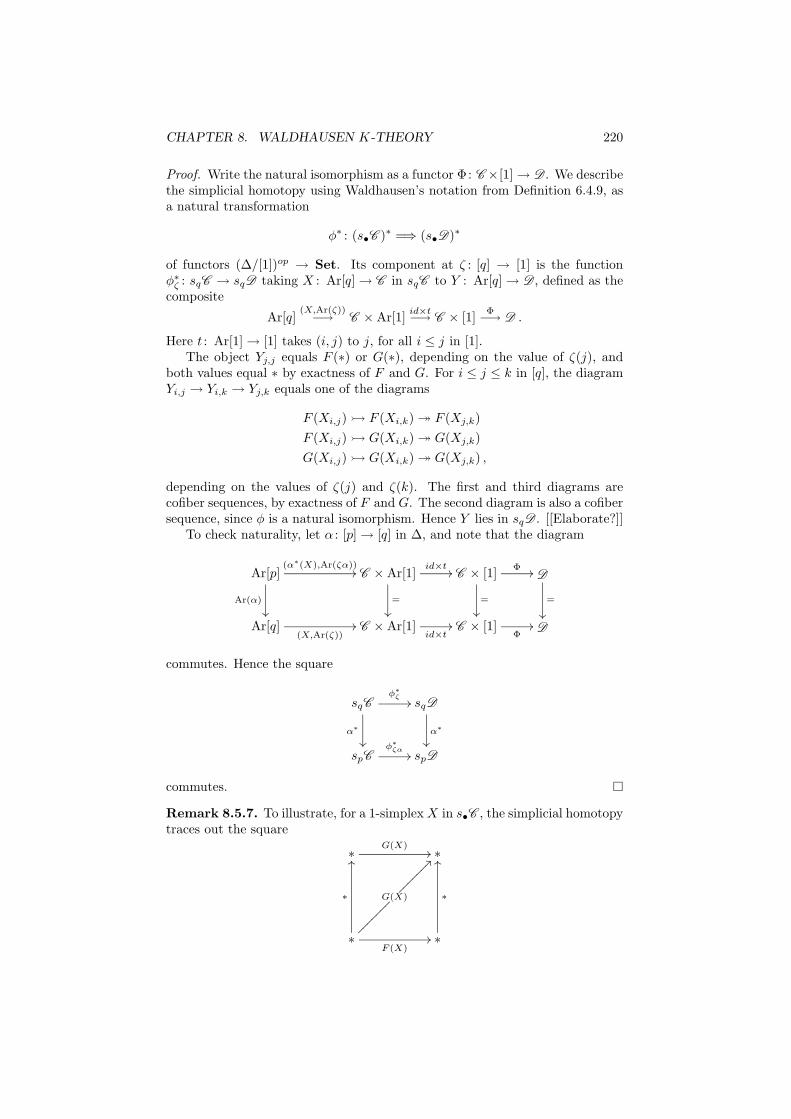
CHAPTER 8. WALDHAUSEN K-THEORY 220
Proof. Write the natural isomorphism as a functor Φ: C ×[1] → D . We describethe simplicial homotopy using Waldhausen’s notation from Definition 6.4.9, asa natural transformation
φ∗ : (s•C )∗ =⇒ (s•D)∗
of functors (∆/[1])op → Set. Its component at ζ : [q] → [1] is the functionφ∗
ζ : sqC → sqD taking X : Ar[q] → C in sqC to Y : Ar[q] → D , defined as thecomposite
Ar[q](X,Ar(ζ))−→ C × Ar[1]
id×t−→ C × [1]
Φ−→ D .
Here t : Ar[1] → [1] takes (i, j) to j, for all i ≤ j in [1].The object Yj,j equals F (∗) or G(∗), depending on the value of ζ(j), and
both values equal ∗ by exactness of F and G. For i ≤ j ≤ k in [q], the diagramYi,j → Yi,k → Yj,k equals one of the diagrams
F (Xi,j) F (Xi,k) ։ F (Xj,k)
F (Xi,j) G(Xi,k) ։ G(Xj,k)
G(Xi,j) G(Xi,k) ։ G(Xj,k) ,
depending on the values of ζ(j) and ζ(k). The first and third diagrams arecofiber sequences, by exactness of F and G. The second diagram is also a cofibersequence, since φ is a natural isomorphism. Hence Y lies in sqD . [[Elaborate?]]
To check naturality, let α : [p] → [q] in ∆, and note that the diagram
Ar[p]
Ar(α)
²²
(α∗(X),Ar(ζα))// C × Ar[1]
id×t//
=
²²
C × [1]Φ //
=
²²
D
=
²²
Ar[q](X,Ar(ζ))
// C × Ar[1]id×t
// C × [1]Φ
// D
commutes. Hence the square
sqCφ∗
ζ//
α∗
²²
sqD
α∗
²²
spCφ∗
ζα// spD
commutes.
Remark 8.5.7. To illustrate, for a 1-simplex X in s•C , the simplicial homotopytraces out the square
∗G(X)
// ∗
∗F (X)
//
∗
OO
G(X)ÄÄÄÄÄÄÄ
??ÄÄÄÄÄÄÄ
∗
∗
OO
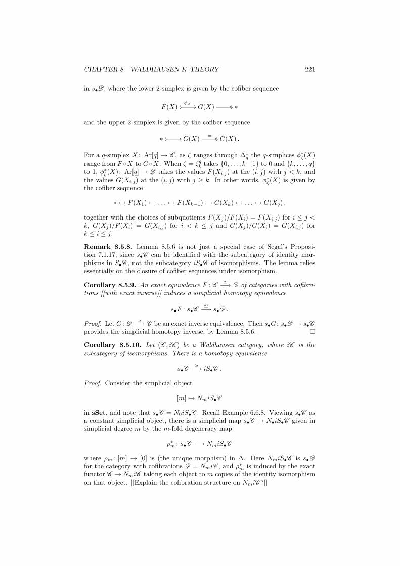
CHAPTER 8. WALDHAUSEN K-THEORY 221
in s•D , where the lower 2-simplex is given by the cofiber sequence
F (X) //φX // G(X) // // ∗
and the upper 2-simplex is given by the cofiber sequence
∗ // // G(X)= // // G(X) .
For a q-simplex X : Ar[q] → C , as ζ ranges through ∆1q the q-simplices φ∗
ζ(X)
range from F X to GX. When ζ = ζqk takes 0, . . . , k−1 to 0 and k, . . . , q
to 1, φ∗ζ(X) : Ar[q] → D takes the values F (Xi,j) at the (i, j) with j < k, and
the values G(Xi,j) at the (i, j) with j ≥ k. In other words, φ∗ζ(X) is given by
the cofiber sequence
∗ F (X1) . . . F (Xk−1) G(Xk) . . . G(Xq) ,
together with the choices of subquotients F (Xj)/F (Xi) = F (Xi,j) for i ≤ j <k, G(Xj)/F (Xi) = G(Xi,j) for i < k ≤ j and G(Xj)/G(Xi) = G(Xi,j) fork ≤ i ≤ j.
Remark 8.5.8. Lemma 8.5.6 is not just a special case of Segal’s Proposi-tion 7.1.17, since s•C can be identified with the subcategory of identity mor-phisms in S•C , not the subcategory iS•C of isomorphisms. The lemma reliesessentially on the closure of cofiber sequences under isomorphism.
Corollary 8.5.9. An exact equivalence F : C≃−→ D of categories with cofibra-
tions [[with exact inverse]] induces a simplicial homotopy equivalence
s•F : s•C≃−→ s•D .
Proof. Let G : D≃−→ C be an exact inverse equivalence. Then s•G : s•D → s•C
provides the simplicial homotopy inverse, by Lemma 8.5.6.
Corollary 8.5.10. Let (C , iC ) be a Waldhausen category, where iC is thesubcategory of isomorphisms. There is a homotopy equivalence
s•C≃−→ iS•C .
Proof. Consider the simplicial object
[m] 7→ NmiS•C
in sSet, and note that s•C = N0iS•C . Recall Example 6.6.8. Viewing s•C asa constant simplicial object, there is a simplicial map s•C → N•iS•C given insimplicial degree m by the m-fold degeneracy map
ρ∗m : s•C −→ NmiS•C
where ρm : [m] → [0] is (the unique morphism) in ∆. Here NmiS•C is s•Dfor the category with cofibrations D = NmiC , and ρ∗m is induced by the exactfunctor C → NmiC taking each object to m copies of the identity isomorphismon that object. [[Explain the cofibration structure on NmiC ?]]
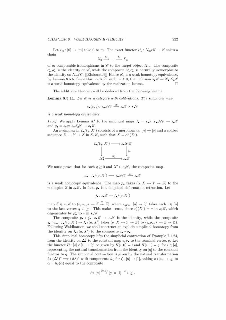
CHAPTER 8. WALDHAUSEN K-THEORY 222
Let ǫm : [0] → [m] take 0 to m. The exact functor ǫ∗m : NmiC → C takes achain
X0
∼=−→ . . .
∼=−→ Xn
of m composable isomorphisms in C to the target object Xm. The compositeǫ∗mρ∗m is the identity on C , while the composite ρ∗mǫ∗m is naturally isomorphic tothe identity on NmiC . [[Elaborate?]] Hence ρ∗m is a weak homotopy equivalence,by Lemma 8.5.6. Since this holds for each m ≥ 0, the inclusion s•C → N•iS•C
is a weak homotopy equivalence by the realization lemma.
The additivity theorem will be deduced from the following lemma.
Lemma 8.5.11. Let C be a category with cofibrations. The simplicial map
s•(s, q) : s•S2C≃−→ s•C × s•C
is a weak homotopy equivalence.
Proof. We apply Lemma A* to the simplicial maps f• = s•s : s•S2C → s•Cand g• = s•q : s•S2C → s•C .
An n-simplex in f•/(q,X ′) consists of a morphism α : [n] → [q] and a cofibersequence X Y ։ Z in SnC , such that X = α∗(X ′).
f•/(q,X ′) //
²²
s•S2C
f•
²²
∆q•
X′• // s•C
We must prove that for each q ≥ 0 and X ′ ∈ sqC , the composite map
p• : f•/(q,X ′) −→ s•S2Cg•−→ s•C
is a weak homotopy equivalence. The map p• takes (α,X Y ։ Z) to then-simplex Z in s•C . In fact, p• is a simplicial deformation retraction. Let
j• : s•C → f•/(q,X ′)
map Z ∈ snC to (ǫqρn, ∗ Z=։ Z), where ǫqρn : [n] → [q] takes each i ∈ [n]
to the last vertex q ∈ [q]. This makes sense, since ǫ∗q(X′) = ∗ in s0C , which
degenerates by ρ∗n to ∗ in snC .The composite p• j• : s•C → s•C is the identity, while the composite
j• p• : f•/(q,X ′) → f•/(q,X ′) takes (α,X Y ։ Z) to (ǫqρn, ∗ Z ։ Z).Following Waldhausen, we shall construct an explicit simplicial homotopy fromthe identity on f•/(q,X ′) to the composite j• p•.
This simplicial homotopy lifts the simplicial contraction of Example 7.1.24,from the identity on ∆q
• to the constant map ǫqρ• to the terminal vertex q. Letthe functor H : [q]× [1] → [q] be given by H(i, 0) = i and H(i, 1) = q, for i ∈ [q],representing the natural transformation from the identity on [q] to the constantfunctor to q. The simplicial contraction is given by the natural transformationh : (∆q)∗ =⇒ (∆q)∗ with components hζ for ζ : [n] → [1], taking α : [n] → [q] toα = hζ(α) equal to the composite
α : [n](α,ζ)−→ [q] × [1]
H−→ [q] .
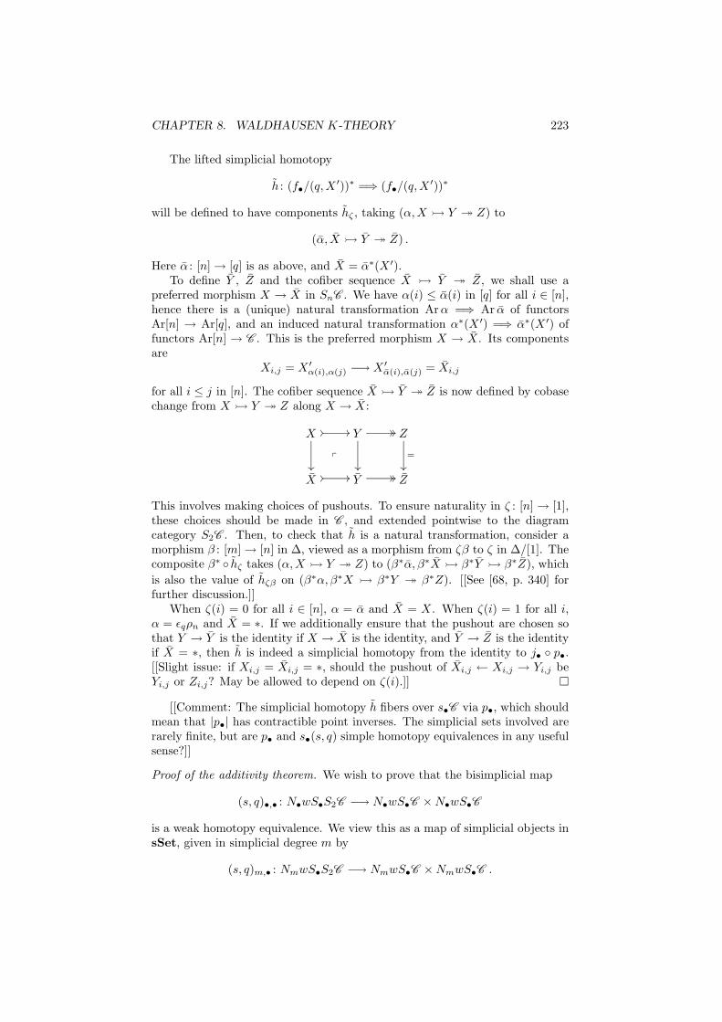
CHAPTER 8. WALDHAUSEN K-THEORY 223
The lifted simplicial homotopy
h : (f•/(q,X ′))∗ =⇒ (f•/(q,X ′))∗
will be defined to have components hζ , taking (α,X Y ։ Z) to
(α, X Y ։ Z) .
Here α : [n] → [q] is as above, and X = α∗(X ′).To define Y , Z and the cofiber sequence X Y ։ Z, we shall use a
preferred morphism X → X in SnC . We have α(i) ≤ α(i) in [q] for all i ∈ [n],hence there is a (unique) natural transformation Arα =⇒ Ar α of functorsAr[n] → Ar[q], and an induced natural transformation α∗(X ′) =⇒ α∗(X ′) offunctors Ar[n] → C . This is the preferred morphism X → X. Its componentsare
Xi,j = X ′α(i),α(j) −→ X ′
α(i),α(j) = Xi,j
for all i ≤ j in [n]. The cofiber sequence X Y ։ Z is now defined by cobasechange from X Y ։ Z along X → X:
X // //
²²
p
Y // //
²²
Z
=
²²
X // // Y // // Z
This involves making choices of pushouts. To ensure naturality in ζ : [n] → [1],these choices should be made in C , and extended pointwise to the diagramcategory S2C . Then, to check that h is a natural transformation, consider amorphism β : [m] → [n] in ∆, viewed as a morphism from ζβ to ζ in ∆/[1]. Thecomposite β∗ hζ takes (α,X Y ։ Z) to (β∗α, β∗X β∗Y β∗Z), which
is also the value of hζβ on (β∗α, β∗X β∗Y ։ β∗Z). [[See [68, p. 340] forfurther discussion.]]
When ζ(i) = 0 for all i ∈ [n], α = α and X = X. When ζ(i) = 1 for all i,α = ǫqρn and X = ∗. If we additionally ensure that the pushout are chosen sothat Y → Y is the identity if X → X is the identity, and Y → Z is the identityif X = ∗, then h is indeed a simplicial homotopy from the identity to j• p•.[[Slight issue: if Xi,j = Xi,j = ∗, should the pushout of Xi,j ← Xi,j → Yi,j beYi,j or Zi,j? May be allowed to depend on ζ(i).]]
[[Comment: The simplicial homotopy h fibers over s•C via p•, which shouldmean that |p•| has contractible point inverses. The simplicial sets involved arerarely finite, but are p• and s•(s, q) simple homotopy equivalences in any usefulsense?]]
Proof of the additivity theorem. We wish to prove that the bisimplicial map
(s, q)•,• : N•wS•S2C −→ N•wS•C × N•wS•C
is a weak homotopy equivalence. We view this as a map of simplicial objects insSet, given in simplicial degree m by
(s, q)m,• : NmwS•S2C −→ NmwS•C × NmwS•C .
CHAPTER 8. WALDHAUSEN K-THEORY 224
For each m ≥ 0, let C (m,w) ⊆ Fun([m],C ) be the full subcategory gener-ated by the functors that takes values in wC , i.e., the diagrams
X0 ∼−→ X1 ∼
−→ . . .∼−→ Xm .
Then C (m,w) is a subcategory with cofibrations of Fun([m],C ), and [m] 7→C (m,w) defines a simplicial category with cofibrations. There are simplicialisomorphisms
NmwS•C∼= s•C (m,w)
andNmwS•S2C
∼= s•S2C (m,w) ,
and the map (s, q)m,• can be rewritten as the map
s•(s, q) : s•S2C (m,w) −→ s•C (m,w) × s•C (m,w)
of Lemma 8.5.11, for the category with cofibrations C (m,w). Hence (s, q)m,• isa weak equivalence for each m ≥ 0, and the bisimplicial map (s, q)•,• is a weakequivalence by the realization lemma.
8.6 Delooping K-theory
[[Introduction, reference to [68, 1.5]]]
Definition 8.6.1. Let P : ∆ → ∆ be the shift functor taking [q] to P [q] =[q + 1] and α : [p] → [q] to Pα : [p + 1] → [q + 1], given by Pα(0) = 0 andPα(i + 1) = α(i) + 1 for i ∈ [p].
Given a simplicial object X• in a category D , i.e., a functor X : ∆op → D ,let the path object PX• be given by the composite functor X P op : ∆op → D ,so that (PX)q = Xq+1 for all q ≥ 0.
The 0-th face maps δq+10 : [q] → [q + 1] induce a natural transformation
id =⇒ P and a simplicial map
d0 : PX• −→ X• ,
given by d0 : PXq = Xq+1 → Xq for each q ≥ 0. The inclusion of zero-simplicesinduces maps X1 = PX0 → PX• and X0 → X•, and the square
X1//
d0
²²
PX•
d0
²²
X0// X•
commutes.
[[Discuss P sing(Y )• as an example.]]
Lemma 8.6.2. There is a simplicial homotopy equivalence PX ≃ X0.
[[See [68, 1.5.1].]]
CHAPTER 8. WALDHAUSEN K-THEORY 225
We apply this when X• = wS•C for a Waldhausen category (C , wC ). ThenX0 = wS0C = ∗ and X1 = wS1C
∼= wC , so we have a diagram of simplicialcategories
wC −→ P (wS•C )d0−→ wS•C , (8.3)
with constant composite. By the lemma above, P (wS•C ) is simplicially con-tractible. A choice of contraction of |P (wS•C )| thus determines a map
ι : |wC | −→ Ω|wS•C | = K(C , w) .
Lemma 8.6.3. The simplicial contraction of P (wS•C ) can be chosen so that ιis (homotopic to) the map from Definition 8.4.2.
[[See [68, 1.5.2].]]In general ι is not a homotopy equivalence, so diagram (8.3) is not a fibra-
tion up to homotopy. This situation improves greatly after applying the S•
construction one more time.
Proposition 8.6.4. Let (C , wC ) be a Waldhausen category. The diagram
wS•C −→ P (wS•S•C )d0−→ wS•S•C
is a fibration up to homotopy. Hence the map
ι : |wS•C |≃−→ Ω|wS•S•C |
is a homotopy equivalence.
[[See [68, 1.5.3].]]
Proof. We may assume that the path object construction acts on the second ofthe two S• constructions. We use the fibration criterion of Proposition 6.8.2. Itsuffices to show that
wS•C −→ P (wS•S•C )qd0−→ wS•SqC
is a fibration up to homotopy for each q ≥ 0, since wS•SqC is connected foreach q. In view of the definition of the path object functor, we can rewrite thisdiagram as
wS•C −→ wS•Sq+1Cd0−→ wS•SqC .
This is the diagram we obtain by applying wS•(−) to
C −→ Sq+1Cd0−→ SqC ,
and we shall use the additivity theorem to see that this is homotopy equivalentto the product fibration obtained by applying wS•(−) to
C −→ C × SqCpr2−→ SqC .
Let η∗1 : Sq+1C → C take X : Ar[q + 1] → C to X0,1. (It is induced by
the morphism η1 : [1] → [q + 1] from Definition 7.1.5.) We get a commutativediagram
C //
=
²²
Sq+1C
τ
²²
d0 // SqC
=
²²
C // C × SqCpr2 // SqC
CHAPTER 8. WALDHAUSEN K-THEORY 226
where τ = (η∗1 , d0) takes an object
X0,1 X0,2 . . . X0,q+1
(plus choices of subquotients) in Sq+1C to
(X0,1,X1,2 . . . X1,q+1)
(plus choices of subquotients) in C × SqC .We can identify C with the full subcategory of Sq+1C where all cofibrations
X0,j−1 X0,j are identities and all subquotients are ∗. Similarly, we canidentify SqC with the full subcategory of Sq+1C where X0,1 = ∗ and the quotientmaps X0,j ։ X1,j are identities. Using these identifications, the exact functorτ : Sq+1C → C × SqC has an exact section σ given by the composite
C × SqC ⊂ Sq+1C × Sq+1C∨
−→ Sq+1C ,
taking (X0,1,X1,2 . . . X1,q+1) (with choices of subquotients) to
X0,1 X0,1 ∨ X1,2 . . . X0,1 ∨ X1,q+1
(with the evident choices of subquotients).The composite τ σ is the identity, while the composite σ τ : Sq+1C →
Sq+1C is the wedge sum of the two exact functors
F ′, F ′′ : Sq+1C → Sq+1C
taking X0,1 X0,2 . . . X0,q+1 to
X0,1=−→ X0,1
=−→ . . .
=−→ X0,1
and∗ X1,2 . . . X1,q+1 ,
respectively. Let F be the identity functor on Sq+1C . Then there is a cofibersequence of exact functors
F ′ F ։ F ′′
with components X0,1 X0,j ։ X1,j . Hence, by the additivity theorem(Corollary 8.5.4), there is a homotopy
wS•σ wS•τ = wS•(F′ ∨ F ′′) ≃ wS•F
to the identity on wS•Sq+1C . It follows that wS•τ is a homotopy equivalence,and we get the commutative diagram
wS•C//
=
²²
wS•Sq+1C
wS•τ≃
²²
d0 // wS•SqC
=
²²
wS•C// wS•C × wS•SqC
pr2 // wS•SqC .
The lower row is clearly a fibration up to homotopy, hence so it the upperrow.
CHAPTER 8. WALDHAUSEN K-THEORY 227
8.7 The iterated S•-construction
We can encode the fact that the algebraic K-theory space K(C , w) = Ω|wS•C |is an infinite loop space in an algebraic K-theory spectrum. To discuss mul-tiplicative properties, it is useful to use Jeff Smith’s notion of a symmetricspectrum, see Hovey–Shipley–Smith [27].
Definition 8.7.1. A symmetric spectrum X (in topological spaces) is a sequencen 7→ Xn of based Σn-spaces, with structure maps σ : Xn ∧ S1 → Xn+1 suchthat the k-fold iterate σk : Xn ∧ Sk → Xn+k is (Σn × Σk)-equivariant for eachn, k ≥ 0. Here Σk acts on Sk = S1 ∧ · · · ∧ S1 by permuting the smash factors,and Σn × Σk is viewed as a subgroup of Σn+k in the obvious way.
A map f : X → Y of symmetric spectra is a sequence n 7→ fn : Xn → Ynof based Σn-equivariant maps, such that the square
Xn ∧ S1fn∧id
//
σ
²²
Yn ∧ S1
σ
²²
Xn+1fn+1
// Yn+1
commutes for each n ≥ 0 Let SpΣ be the category of symmetric spectra.
[[Level equivalence, stable equivalence.]]The following constructions are discussed in [68, p. 330] and [57, §1]. The
symmetric structure is emphasized in [21, §6].
Definition 8.7.2. Let (C , wC ) be a Waldhausen category. The external n-foldS•-construction on C is the n-multisimplicial Waldhausen category
(S• . . . S•C , wS• . . . S•C ) .
In multidegree (q1, . . . , qn), it has objects the Ar[q1] × · · · × Ar[qn]-shaped dia-grams
X : Ar[q1] × · · · × Ar[qn] −→ C
such that
(a)X(i1 ≤ j1, . . . , in ≤ jn) = ∗
if it = jt in [qt] for some 1 ≤ t ≤ n.
(b)X(. . . , it ≤ jt, . . . ) X(. . . , it ≤ kt, . . . ) ։ X(. . . , jt ≤ kt, . . . )
is a cofiber sequence in the (n− 1)-fold iterated S•-construction, for eachtriple it ≤ jt ≤ kt in [qt].
Let the internal n-fold S•-construction
(S(n)• C , wS
(n)• C )
be the diagonal simplicial Waldhausen category, with q-simplices
(S(n)q C , wS(n)
q C ) = (Sq . . . SqC , wSq . . . SqC ) .
CHAPTER 8. WALDHAUSEN K-THEORY 228
It has objects the (Ar[q])n = Ar([q]n)-shaped diagrams
X : Ar[q]n −→ C
such that
(a)X(i1 ≤ j1, . . . , in ≤ jn) = ∗
if it = jt in [q] for some 1 ≤ t ≤ n.
(b)X(. . . , it ≤ jt, . . . ) X(. . . , it ≤ kt, . . . ) ։ X(. . . , jt ≤ kt, . . . )
is a cofiber sequence in the (n− 1)-fold iterated S•-construction, for eachtriple it ≤ jt ≤ kt in [q].
The symmetric group Σn acts simplicially on S(n)• C , by permuting the n
copies of [q] in Ar[q]n. More explicitly, for π ∈ Σn,
(π · X)(. . . , it ≤ jt, . . . ) = X(. . . , iπ−1(t) ≤ jπ−1(t), . . . ) .
Definition 8.7.3. The (symmetric) algebraic K-theory spectrum K(C , w) of asmall Waldhausen category (C , wC ) has n-th space
K(C , w)n = |wS(n)• C |
based at ∗, with the Σn-action induced by permuting the order of the S•-constructions. The structure map σ is the composite
|wS(n)• C | ∧ S1 ∼= |wS
(n)• S•C |(1) ⊂ |wS
(n)• S•C | ∼= |wS
(n+1)• C | ,
where the superscript (1) indicates the 1-skeleton with respect to the last simpli-cial direction. See Lemma 8.4.1. The k-fold iterated structure map σk is thenthe composite
|wS(n)• C | ∧ Sk ∼= |wS
(n)• S• . . . S•C |(1,...,1) ⊂ |wS
(n)• S• . . . S•C | ∼= |wS
(n+k)• C | ,
where the superscript (1,...,1) indicates the multi-1-skeleton with respect to thek last simplicial directions. This map is clearly (Σn × Σk)-equivariant.
Lemma 8.7.4. The algebraic K-theory spectrum is positively fibrant (= a semi-Ω-spectrum), in the sense that the adjoint structure maps
K(C , w)n≃−→ ΩK(C , w)n+1
are homotopy equivalences for all n ≥ 1. Hence there are isomorphisms
Ki(C , w) = πi+1K(C , w)1 ∼= πiK(C , w)
for all i ≥ 0.
Proof. This is the map ι : |wS•D | → Ω|wS•S•D | for D = S(n−1)• C , which is a
homotopy equivalence by Proposition 8.6.4.
Remark 8.7.5. We can also define K(C , w) as a symmetric spectrum in sim-
plicial sets, letting K(C , w)n be the diagonal of N•wS(n)• C . Note that this is
not a fibrant simplicial set (= a Kan complex) in most cases.
[[Reference for model structures?]][[Biexact functors D ×E → C induce pairing K(D)∧K(E ) → K(C ), taking
wS(m)• D × wS
(n)• E to wS
(m+n)• C . Swallowing lemma.]]
CHAPTER 8. WALDHAUSEN K-THEORY 229
8.8 The spectrum level rank filtration
[[Reference to [57].]]
Definition 8.8.1. Let C be a small category with cofibrations. We call
rank: obj(C ) → N0 = 0, 1, 2, . . .
a rank function if
(a) rank(X) = 0 if and only if X ∼= ∗ is a zero object.
(b) If f : X Y is a cofibration then rank(X) ≤ rank(Y ), with rank(X) =rank(Y ) only if f is an isomorphism.
(c) If f : X Y is a cofibration then rank(Y ) ≥ rank(Y/X), with rank(Y ) =rank(Y/X) only if X ∼= ∗.
Remark 8.8.2. If f : X∼=−→ Y is an isomorphism, then f and f−1 are cofibra-
tions, so rank(X) ≤ rank(Y ) and rank(Y ) ≤ rank(X), so rank(X) = rank(Y ).
Example 8.8.3. For a commutative ring R, let C = F (R) be the categoryof finitely generated free R-modules, with split injective cofibrations, and letrank(Rk) = k. [[This also works for certain reasonable, non-commutative rings.]]
Example 8.8.4. Let C = F∗ be the category of finite pointed sets, withinjective cofibrations, and let rank(k+) = k, where k+ = 0, 1, 2, . . . , k is basedat 0.
We consider the algebraic K-theory K(C ) = K(C , iC ) of C with respect tothe subcategory iC = iso(C ) of weak equivalences.
Definition 8.8.5. For each k ≥ 0 let FkC ⊂ C be the full pointed subcategorygenerated by the objects X with rank(X) ≤ k. For each level n ≥ 0 and degreeq ≥ 0 let
FkiS(n)q C ⊂ iS(n)
q C
be the full pointed subgroupoid generated by the objects X : Ar[q]n → C in
S(n)q C that factor through FkC ⊂ C . Then FkiS
(n)• C ⊂ iS
(n)• C is a simplicial
pointed subgroupoid, and we let
FkK(C ) ⊂ K(C )
be the symmetric subspectrum with n-th space
FkK(C )n = |FkiS(n)• C | ⊂ |iS
(n)• C | = K(C )n .
It is clear that the Σn-action on K(C )n restricts to FkK(C )n, and that thestructure maps σ : K(C )n ∧ S1 → K(C )n+1 restrict to σ : FkK(C )n ∧ S1 →FkK(C )n+1, satisfying the required equivariance property.
As k varies, we obtain a diagram of symmetric spectra
F0K(C ) F1K(C ) . . . Fk−1K(C ) FkK(C ) . . . K(C )
where each map is a levelwise cofibration, and colimk FkK(C ) ∼= K(C ). This isthe spectrum level rank filtration of K(C ). In particular,
colimk
πiFkK(C )∼=−→ Ki(C )
for all i ≥ 0.
CHAPTER 8. WALDHAUSEN K-THEORY 230
Lemma 8.8.6. There is a levelwise equivalence F0K(C ) ≃ ∗.
Proof. By condition (a) in the definition of a rank function, F0iS(n)q C is the
pointed groupoid of diagrams X : Ar[q]n → F0C , all uniquely isomorphic to the
constant diagram at the chosen zero object ∗. Hence F0iS(n)q C is contractible for
each q, so |F0iS(n)• C | = F0K(C )n is contractible by the realization lemma.
Lemma 8.8.7. Let k ≥ 1. An object X : Ar[q]n → C in S(n)q C lies in FkiS
(n)q C
but not in Fk−1iS(n)q C if and only if
rankX(0 ≤ q, . . . , 0 ≤ q) = k .
Proof. In view of the cofibration
X(0 ≤ j1, . . . , 0 ≤ jn) X(0 ≤ q, . . . , 0 ≤ q)
and quotient map [[Explain?]]
X(0 ≤ j1, . . . , 0 ≤ jn) ։ X(i1 ≤ j1, . . . , in ≤ jn)
it is clear that
rankX(i1 ≤ j1, . . . , in ≤ jn) ≤ X(0 ≤ q, . . . , 0 ≤ q)
for all (i1 ≤ j1, . . . , in ≤ jn) in Ar[q]n. Hence X factors through FkC if andonly if rankX(0 ≤ q, . . . , 0 ≤ q) ≤ k.
Definition 8.8.8. For each object X : Ar[q]n → C in S(n)q C we call
X(0 ≤ q, . . . , 0 ≤ q)
the top object of X. Its rank is the top rank of X.
Definition 8.8.9. For k ≥ 1, let
FkK(C ) = FkK(C )/Fk−1K(C )
be the k-th subquotient spectrum in the rank filtration. It has n-th space
FkK(C )n = |FkiS(n)• C | where
FkiS(n)• C = FkiS
(n)• C /Fk−1iS
(n)• C
is the simplicial pointed groupoid obtained from FkiS(n)• C by identifying all
X : Ar[q]n → C with top rank < k to the base point object, with trivial auto-morphism group.
In simplicial degree q, the pointed groupoid FkiS(n)q C has objects the base
point, together with the diagrams X : Ar[q]n → C in S(n)q C with top rank k.
For each α : [p] → [q] the simplicial operator α∗ takes X to
X Ar(α)n : Ar[p]n → C
in S(n)p C whenever this has top rank k, and to the base point object otherwise.
Note that if α(0) = a and α(p) = b, then the top object of X Ar(α)n isX(a ≤ b, . . . , a ≤ b).
CHAPTER 8. WALDHAUSEN K-THEORY 231
Definition 8.8.10. The embedding [q] → Ar[q] induces embeddings [q]n →Ar[q]n taking (j1, . . . , jn) to (0 ≤ j1, . . . , 0 ≤ jn), for all n ≥ 0. The n-dimensional cube [q]n is partially ordered with the product ordering, so thatu = (i1, . . . , in) and v = (j1, . . . , jn) satisfy u ≤ v if and only if i1 ≤ j1, . . . , in ≤jn. For X : Ar[q]n → C let its restriction
X : [q]n → C
be the composite [q]n → Ar[q]n → C . The top object of X is the top object
X(q, . . . , q) = X(0 ≤ q, . . . , 0 ≤ q)
of X.
Definition 8.8.11. We say that X : [q]n → C is a lattice (n-)cube if
(a) X(i1, . . . , in) = ∗ whenever some it = 0, 1 ≤ t ≤ n.
(b) For each v ∈ [q]n the canonical map
colimu<v
X(u) X(v)
is a cofibration in C , where the colimit ranges over the u ∈ [q]n that arestrictly smaller than v in the product partial ordering.
[[Explain why the colimit exists, by induction on v.]]
Lemma 8.8.12. A diagram X : [q]n → C is the restriction of an object X in
S(n)q C if and only if X is a lattice cube.
Proof. For n = 1, an object X : Ar[q] → C in SqC consists of a sequence
X0 −→ X1 −→ . . . −→ Xq
in C , where X0 = ∗ and each Xi−1 Xi is a cofibration, together withcompatible choices of quotients X(i ≤ j) ∼= Xj/Xi. The restriction X 7→ Xforgets the choices of quotients.
For n = 2, an object X : Ar[q]2 → C in S(2)q C consists of a q × q square
X0,q // X1,q // . . . // Xq,q
...
OO
...
OO
...
OO
X0,1 //
OO
X1,1 //
OO
. . . // Xq,1
OO
X0,0 //
OO
X1,0 //
OO
. . . // Xq,0
OO
in C , where Xi1,0 = X0,i2 = ∗ and each pushout morphism
Xi1,i2−1 ∪Xi1−1,i2−1Xi1−1,i2 Xi1,i2
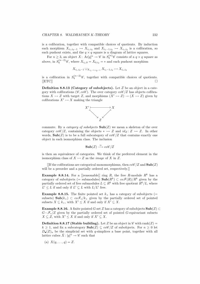
CHAPTER 8. WALDHAUSEN K-THEORY 232
is a cofibration, together with compatible choices of quotients. By inductioneach morphism Xi1,i2−1 Xi1,i2 and Xi1−1,i2 Xi1,i2 is a cofibration, soeach pushout exists, and the q × q square is a diagram of lattice squares.
For n ≥ 3, an object X : Ar[q]n → C in S(n)q C consists of a q × q square as
above, in S(n−2)q C , where Xi1,0 = X0,i2 = ∗ and each pushout morphism
Xi1,i2−1 ∪Xi1−1,i2−1Xi1−1,i2 Xi1,i2
is a cofibration in S(n−2)q C , together with compatible choices of quotients.
[[ETC]]
Definition 8.8.13 (Category of subobjects). Let Z be an object in a cate-gory with cofibrations (C , coC ). The over category coC /Z has objects cofibra-tions X Z with target Z, and morphisms (X ′
Z) → (X Z) given bycofibrations X ′
X making the triangle
X ′ // //ÃÃ
ÃÃAA
AAAA
AX
ÄÄ
ÄÄ~~~~
~~~
Z
commute. By a category of subobjects Sub(Z) we mean a skeleton of the overcategory coC /Z, containing the objects ∗ Z and idZ : Z Z. In otherwords, Sub(Z) is to be a full subcategory of coC /Z that contains exactly oneobject in each isomorphism class. The inclusion
Sub(Z)≃−→ coC /Z
is then an equivalence of categories. We think of the preferred element in theisomorphism class of X Z as the image of X in Z.
[[If the cofibrations are categorical monomorphisms, then coC /Z and Sub(Z)will be a preorder and a partially ordered set, respectively.]]
Example 8.8.14. For a [[reasonable]] ring R, the free R-module Rk has acategory of subobjects (= submodules) Sub(Rk) ⊂ coF (R)/Rk given by thepartially ordered set of free submodules L ⊆ Rk with free quotient Rk/L, whereL′ ≤ L if and only if L′ ⊆ L with L/L′ free.
Example 8.8.15. The finite pointed set k+ has a category of subobjects (=subsets) Sub(k+) ⊂ coF∗/k+ given by the partially ordered set of pointedsubsets X ⊆ k+, with X ′ ≤ X if and only if X ′ ⊆ X.
Example 8.8.16. A finite pointed G-set Z has a category of subobjects Sub(Z) ⊂G−F∗/Z given by the partially ordered set of pointed G-equivariant subsetsX ⊆ Z, with X ′ ≤ X if and only if X ′ ⊆ X.
Definition 8.8.17 (Stable building). Let Z be an object in C with rank(Z) =k ≥ 1, and fix a subcategory Sub(Z) ⊆ coC /Z of subobjects. For n ≥ 0 letD•(Z)n be the simplicial set with q-simplices a base point, together with alllattice cubes X : [q]n → C such that
(a) X(q, . . . , q) = Z.
CHAPTER 8. WALDHAUSEN K-THEORY 233
(b) X(v) Z is an object in Sub(Z), for each v ∈ [q]n.
For α : [p] → [q] in ∆ the simplicial operator α∗ : Dq(Z)n → Dp(Z)n takes Xto Y = X αn if Y (i1, . . . , in) = ∗ whenever some it = 0 and Y (p, . . . , p) = Z,and to the base point otherwise.
The stable building D(Z) is the symmetric spectrum with n-th space D(Z)n =|D•(Z)n|. [[Evident symmetric group action and spectrum structure maps.]]
[[The automorphism group Aut(Z) of Z acts naturally on D(Z).]]
Example 8.8.18. For a [[reasonable]] ring R, the q-simplices of D•(Rk)n are
the base point, together with the diagrams X : [q]n → F (R) such that
(a) X(i1, . . . , in) = 0 whenever some it = 0.
(b) X(q, . . . , q) = Rk.
(c) X(u) → X(v) is an inclusion of free R-modules, with free quotient, foreach u ≤ v in [q]n.
(d) colimu<v X(u) X(v) is injective with free quotient, for each v ∈ [q]n.
Example 8.8.19. The q-simplices of D•(k+)n are the base point, together withthe diagrams X : [q]n → F∗ such that
(a) X(i1, . . . , in) = 0+ whenever some it = 0.
(b) X(q, . . . , q) = k+.
(c) X(u) → X(v) is an inclusion of pointed sets for each u ≤ v in [q]n.
(d) colimu<v X(u) X(v) is injective for each v ∈ [q]n.
[[Also G-sets?]]
Proposition 8.8.20. There is a levelwise equivalence
FkK(C ) ≃∨
Z
E Aut(Z)+ ∧Aut(Z) D(Z)
of symmetric spectra, where the wedge sum runs over representatives for theisomorphism classes of objects of rank k in C , and Aut(Z) is the automorphismgroup of Z.
Proof. Step 1: Let Eq ⊂ FkiS(n)q C be the full subgroupoid generated by the
base point object, together with the X : Ar[q]n → C such that each quotientmap
X(u ≤ w) ։ X(v ≤ w)
that is an isomorphism is actually an identity morphism, for all u ≤ v ≤ w in
[q]n. Each object in FkiS(n)q C is isomorphic to an object in the subgroupoid,
so the inclusion is an equivalence of categories. [[For each fixed w, choose theX(u ≤ w) appropriately for increasing u.]]
The simplicial operators respect the subgroupoids, hence these assemble to a
simplicial pointed groupoid E•, and the inclusion E• ⊂ FkiS(n)• C is a homotopy
equivalence by the realization lemma.
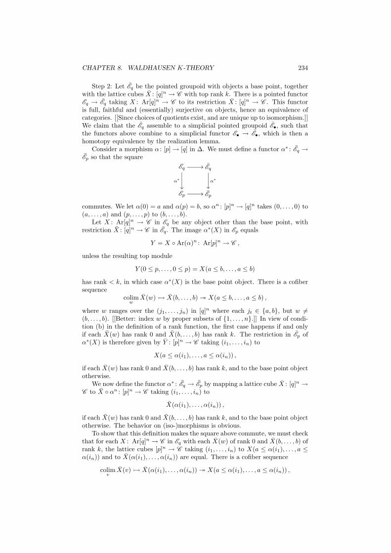
CHAPTER 8. WALDHAUSEN K-THEORY 234
Step 2: Let Eq be the pointed groupoid with objects a base point, togetherwith the lattice cubes X : [q]n → C with top rank k. There is a pointed functorEq → Eq taking X : Ar[q]n → C to its restriction X : [q]n → C . This functoris full, faithful and (essentially) surjective on objects, hence an equivalence ofcategories. [[Since choices of quotients exist, and are unique up to isomorphism.]]We claim that the Eq assemble to a simplicial pointed groupoid E•, such thatthe functors above combine to a simplicial functor E• → E•, which is then ahomotopy equivalence by the realization lemma.
Consider a morphism α : [p] → [q] in ∆. We must define a functor α∗ : Eq →Ep so that the square
Eq//
α∗
²²
Eq
α∗
²²
Ep// Ep
commutes. We let α(0) = a and α(p) = b, so αn : [p]n → [q]n takes (0, . . . , 0) to(a, . . . , a) and (p, . . . , p) to (b, . . . , b).
Let X : Ar[q]n → C in Eq be any object other than the base point, withrestriction X : [q]n → C in Eq. The image α∗(X) in Ep equals
Y = X Ar(α)n : Ar[p]n → C ,
unless the resulting top module
Y (0 ≤ p, . . . , 0 ≤ p) = X(a ≤ b, . . . , a ≤ b)
has rank < k, in which case α∗(X) is the base point object. There is a cofibersequence
colimw
X(w) X(b, . . . , b) ։ X(a ≤ b, . . . , a ≤ b) ,
where w ranges over the (j1, . . . , jn) in [q]n where each jt ∈ a, b, but w 6=(b, . . . , b). [[Better: index w by proper subsets of 1, . . . , n.]] In view of condi-tion (b) in the definition of a rank function, the first case happens if and onlyif each X(w) has rank 0 and X(b, . . . , b) has rank k. The restriction in Ep ofα∗(X) is therefore given by Y : [p]n → C taking (i1, . . . , in) to
X(a ≤ α(i1), . . . , a ≤ α(in)) ,
if each X(w) has rank 0 and X(b, . . . , b) has rank k, and to the base point objectotherwise.
We now define the functor α∗ : Eq → Ep by mapping a lattice cube X : [q]n →C to X αn : [p]n → C taking (i1, . . . , in) to
X(α(i1), . . . , α(in)) ,
if each X(w) has rank 0 and X(b, . . . , b) has rank k, and to the base point objectotherwise. The behavior on (iso-)morphisms is obvious.
To show that this definition makes the square above commute, we must checkthat for each X : Ar[q]n → C in Eq with each X(w) of rank 0 and X(b, . . . , b) ofrank k, the lattice cubes [p]n → C taking (i1, . . . , in) to X(a ≤ α(i1), . . . , a ≤α(in)) and to X(α(i1), . . . , α(in)) are equal. There is a cofiber sequence
colimv
X(v) X(α(i1), . . . , α(in)) ։ X(a ≤ α(i1), . . . , a ≤ α(in)) ,
CHAPTER 8. WALDHAUSEN K-THEORY 235
where v ranges over the (j1, . . . , jn) in [q]n where each jt ∈ a, α(it), butv 6= (α(i1), . . . , α(in)). [[Better: index v by proper subsets of 1, . . . , n.]] Foreach v there is a w as above with v ≤ w, so each X(v) has rank 0 and the colimitis a zero object. Hence the quotient map is an isomorphism by condition (c)in the definition of a rank function, and therefore is an identity map by thedefinition of E•.
It is now easy to check that (βα)∗ = α∗β∗ for any other morphism β : [q] →[r] in ∆, so E• → E• is a well-defined simplicial functor.
Step 3: Each lattice cube X : [q]n → C factors uniquely through coC ⊆ C .If X(q, . . . , q) = Z, then for each v ∈ [q]n the chosen morphisms X(v) Z liftX through coC /Z → coC .
For each object Z of rank k, let Dq(Z) ⊆ Eq be the full subgroupoid generatedby the lattice cubes X : [q]n → C with top object X(q, . . . , q) = Z, such thatthe preferred lift [q]n → coC /Z factors through Sub(Z) ⊆ coC /Z. In otherwords, Dq(Z) is the pointed groupoid with objects a base point, together withthe lattice cubes X : [q]n → C such that X(q, . . . , q) = Z and each X(v) is asubobject of Z.
The (iso-)morphisms X ′ ∼= X are determined by the automorphism f : Z =X ′(q, . . . , q) ∼= X(q, . . . , q) = Z, since then X ′(v) is the image of the composite
X ′(v) Zf
−→ Z
for all v ∈ [q]n. The base point object admits only the identity automorphism.Hence Dq(Z) is the based translation groupoid for the action of Aut(Z) on theobject set obj(Dq(Z)). In particular,
|Dq(Z)| ∼= E Aut(Z)+ ∧Aut(Z) obj(Dq(Z)) .
Letting q ≥ 0 vary, D•(Z) ⊆ E• is a simplicial full subgroupoid. To see thatα∗ : Eq → Ep takes Dq(Z) to Dp(Z), consider a lattice cube X : [q]n → Sub(Z)with top object Z, and let b = α(p). If the top object X(b, . . . , b) of X αn hasrank < k, then α∗(X) is the base point object. Otherwise,
X(b, . . . , b) X(q, . . . , q) = Z
is an isomorphism by condition (c) in the definition of a rank function, henceit equals the identity since Sub(Z) is skeletal and contains idZ : Z Z.Thus α∗(X) is an object in Dp(Z). It follows that D•(Z) is the simplicialbased translation groupoid for the action of Aut(Z) on the simplicial object setobj(D•(Z)) = D•(Z)n. Hence
|D•(Z)| ∼= E Aut(Z)+ ∧Aut(Z) D(Z)n .
Letting Z range over the isomorphism classes of objects of rank k in C , thefull inclusion ∨
Z
D•(Z)≃−→ E•
is a degreewise equivalence of pointed groupoids, since each lattice cube X : [q]n →C in Eq is isomorphic to a lattice cube in Dq(Z) for a unique Z. By the real-ization lemma, we get a homotopy equivalence of simplicial pointed groupoids.
CHAPTER 8. WALDHAUSEN K-THEORY 236
Hence there is a chain of homotopy equivalences
FkK(C )n = |FkiS(n)• C |
≃←− |E•|
≃−→ |E•|
≃←−
∨
Z
|D•(Z)| ∼=∨
Z
E Aut(Z)+ ∧Aut(Z) D(Z)n .
These are compatible with the evident Σn-actions and the spectrum struc-ture maps, leding to the asserted levelwise equivalence.
Corollary 8.8.21. There is a levelwise equivalence
FkK(F (R)) ≃ EGLk(R)+ ∧GLk(R) D(Rk)
of symmetric spectra, for each k ≥ 1.
8.9 Algebraic K-theory of finite sets
[[Using spectrum level rank filtration [57].]]
Proposition 8.9.1. D(k+)n∼= Skn for all k ≥ 1, n ≥ 1.
Proof. Consider first the case k = 1 and n = 1, recalling Exercise 6.3.12. Aq-simplex in D•(1+)1 is a diagram X : [q] → Sub(1+), taking the values 0+ or1+ at each vertex, such that X(j − 1) ⊆ X(j) for each j. If X(0) = 1+ 6= 0+ orX(q) = 0+ 6= 1+, we identify X with the base point. For each such chain
X0 ⊆ X1 ⊆ · · · ⊆ Xq
of pointed subsets of 1+ there is a unique i, with 0 ≤ i ≤ q + 1, such thatXj = 1+ if and only if i ≤ j. The end cases i = 0 and i = q + 1 are thenidentified with the base point, since they correspond to the cases X(0) = 1+
and X(q) = 0+, respectively. Each such chain also corresponds to a morphismζ : [q] → [1] in ∆, or a q-simplex in ∆1
•, via the formula Xj = ζ(j)+. The caseX(0) = 1+ then corresponds to the constant morphism ζ to 1, while the caseX(q) = 0+ corresponds to the constant morphism ζ to 0. Thus the ζ in thesimplicial subset ∂∆1
• ⊂ ∆1• are collapsed to the base point. There is therefore
a simplicial isomorphism
D•(1+)1 ∼= ∆1•/∂∆1
• = S1• .
Next consider the case k = 1 and n ≥ 1. A q-simplex in D•(1+)n is a diagramX : [q]n → Sub(1+), still taking the values 0+ or 1+ at each vertex, subject tothe lattice conditions. These ensure that there exists a unique u = (i1, . . . , in)with 0 ≤ it ≤ q + 1 for each t, such that X(v) = 1+ if and only if u ≤ v. To seethis, consider two vertices v, v′ in [q]n with X(v) = X(v′) = 1+, let u ∈ [q]n bemaximal with u ≤ v, u ≤ v′, and let w ∈ [q]n be minimal with v ≤ w, v′ ≤ w.Clearly then X(w) = 1+. There is then a lattice square
X(v) // X(w)
X(u) //
OO
X(v′) ,
OO
CHAPTER 8. WALDHAUSEN K-THEORY 237
which means that X(u) cannot be 0+, since 1+ ∪0+1+
∼= 2+ does not map bya cofibration to 1+. Hence X(u) = 1+.
Writing u = (i1, . . . , in), each it corresponds to a q-simplex ζt : [q] → [1] in∆1
•, given by ζt(j) = 1 if and only if j ≥ it. The n-tuple (ζ1, . . . , ζn) correspondsto a q-simplex in ∆1
•×· · ·×∆1•. However, if it = 0 or it = q +1 for some t, then
ζt is constant at 0 or 1, and the q-simplex is identified with the base point, dueto the boundary conditions. This means that there is a simplicial isomorphism
D•(1+)n∼= S1
• ∧ · · · ∧ S1• = Sn
• .
In the general case, k ≥ 1 and n ≥ 1, a q-simplex in D•(k+)n is a diagramX : [q]n → Sub(k+), taking values that are pointed subsets of k+ at each vertex,subject to the lattice conditions. These conditions are independent for eachelement s in k+, so X can be viewed as a k-tuple of diagrams X1, . . . , Xk : [q]n →Sub(1+), where Xs(v) = 1+ if and only if s ∈ X(v). We have X(v) = 0+ ifand only if each Xs(v) = 0+, and X(v) = k+ if and only if each Xs(v) = 1+.Hence there is a simplicial isomorphism
D•(k+)n∼= D•(1+)n ∧ · · · ∧ D•(1+)n ,
and D(k+)n∼= D(1+)n ∧ · · · ∧ D(1+)n
∼= Sn ∧ · · · ∧ Sn ∼= Skn.
Corollary 8.9.2. D(1+) ∼= S is the sphere spectrum n 7→ Sn, while D(k+) ≃∗ is stably trivial for k ≥ 2.
Proof. It is easy to check that Σn permutes the n simplicial circles in D•(1+)n∼=
Sn• , and that the spectrum structure map is the usual identification Sn ∧ S1 ∼=
Sn+1.For k ≥ 2, the n-th space D(k+)n
∼= Skn is at least (2n − 1)-connected,hence πi+n(D(k+)n) = 0 for all n > i, so πiD(k+) = 0 in all degrees i. Thisimplies that D(k+) is stably trivial.
We can now prove that the algebraic K-theory of finite sets is the spherespectrum, which is one form of the Barratt–Priddy–Quillen theorem.
Theorem 8.9.3.K(F∗) ≃ S ,
so Ki(F∗) ∼= πi(S) = colimm πi+m(Sm) for all i ≥ 0.
Proof. By Proposition 8.8.20, there are levelwise equivalences
FkK(F∗) ≃ EΣk+ ∧ΣkD(k+)
for k ≥ 1. For k = 1 we get levelwise equivalences F1K(F∗) ≃ F1K(F∗) ≃D(1+) ∼= S, while for k ≥ 2 we get stable equivalences FkK(F∗) ≃ EΣk+∧Σk
∗ ≃∗. It follows that Fk−1K(F∗) → FkK(F∗) is a stable equivalence for each k ≥ 2,hence in the colimit F1K(F∗) → K(F∗) is a stable equivalence.
Corollary 8.9.4. K(F∗)n ≃ Q(Sn) = colimm ΩmSn+m for all n ≥ 0. In par-ticular, for n = 0 the loop space completion map ι : |iF∗| → K(F∗) is homotopyequivalent to
∐n≥0 BΣn → Q(S0).
CHAPTER 8. WALDHAUSEN K-THEORY 238
[[The rank ≤ 1 inclusion S0 ≃ BΣ1+ ⊂∐
n≥0 BΣn → K(F∗)0 is rightadjoint to the spectrum map S → K(F∗) that is an equivalence.]]
[[The map∐
n≥0 BΣn → Q(S0) has interesting geometric constructions, in-volving operads, and induces a homology isomorphism after inverting the gener-ator of H0(BΣ1) in H∗(
∐n≥0 BΣn). Hence there is an equivalence Z×BΣ+
∞ ≃
Q(S0).]]
Corollary 8.9.5 (May–Milgram filtration). For n ≥ 1 there is a filtration
∗ ≃ F0,n . . . Fk−1,n Fk,n . . . K(F∗)n ≃ Q(Sn)
with filtration quotients
Fk,n/Fk−1,n ≃ EΣk+ ∧ΣkSnk
for k ≥ 1, where Σk permutes the copies of Sn in Snk ∼= Sn ∧ · · · ∧ Sn.
Proof. Let Fk,n = FkK(F∗)n.
Definition 8.9.6. For G a finite group, let G−F∗ be the category of finitepointed G-sets and G-equivariant base-point preserving functions. Let coG−F∗
be the subcategory of injective functions, and let rank(X+) = k when X ∼=∐ks=1 G/Hi is the disjoint union of k orbits.
The following is a form of the Segal–tom Dieck splitting. [[reference]]
Theorem 8.9.7.K(G−F∗) ≃
∨
(H)
S[BWG(H)] ,
where the wedge sum runs over the conjugacy classes of subgroups H of G, andWG(H) = NG(H)/H is the Weyl group of H in G, where NG(H) = n ∈ G |nH = Hn is the normalizer of H in G.
Proof. The finite pointed G-sets of rank 1 are of the form G/H+, as H rangesover all subgroups of G. There is an isomorphism G/H ∼= G/K taking eHto cK if and only if H = cKc−1, i.e., if H and K are conjugate subgroups.The automorphism group of Z = G/H+ consists of the G-equivariant func-tions G/H → G/H taking eH to nH, where n ∈ G must normalize H andis only defined modulo H, so Aut(Z) ∼= WG(H). Hence by Lemma 8.8.6 andProposition 8.8.20 for k = 1, there is an equivalence
F1K(G−F∗) ≃∨
(H)
EWG(H)+ ∧WG(H) D(G/H+) .
We claim that there is an isomorphism D(G/H+) ∼= D(1+) ∼= S, with thetrivial WG(H)-action. For any diagram X : [q]n → Sub(G/H+) takes the val-ues ∗ and G/H+ only, of rank 0 and 1, respectively. Hence the isomorphismSub(G/H+) ∼= Sub(1+) taking ∗ and G/H+ to 0+ and 1+, respectively, inducesthe claimed isomorphism. Thus
F1K(G−F∗) ≃∨
(H)
S[BWG(H)] .
CHAPTER 8. WALDHAUSEN K-THEORY 239
More generally, we claim that there is an isomorphism D(Z+) ∼= D(k+) ≃ ∗
for any Z ∼=∐k
s=1 G/Hs. Again, any subobject of Z+ has the form X+, whereX is the coproduct of a subset of the s with 1 ≤ s ≤ k, and the isomor-phism Sub(Z+) ∼= Sub(k+) taking X+ with X =
∐s∈U G/Hs to U+ with
U ⊆ 1, . . . , k induces the claimed isomorphism. Hence by Proposition 8.8.20for k ≥ 2, there is are stable equivalences
FkK(G−F∗) ≃∨
Z
E Aut(Z)+ ∧Aut(Z) D(k+) ≃ ∗ ,
so that all of the maps
F1K(G−F∗)≃−→ . . .
≃−→ Fk−1K(G−F∗)
≃−→ Fk−1K(G−F∗)
≃−→ . . .
≃−→ K(G−F∗)
are stable equivalences.
[[Note how K0(G−F∗) ∼=∐
(H) Z ∼= A(G) is the free abelian group generated
by the G/H, i.e., the Burnside ring.]][[The rank ≤ 1 inclusion (
∐(H) BWG(H))+ ⊂ |i(G−F∗)| → K(G−F∗) is
right adjoint to the spectrum map∨
(H) S[BWG(H)] → K(G−F∗) that is an
equivalence.]][[One can also identify K(G−F∗) with the G-fixed point spectrum (SG)G of
the G-equivariant sphere spectrum SG. The loop space completion map takes|i(G−F∗)| ≃
∐[Z] B Aut(Z) to QG(S0)G = colimV (ΩV SV )G where V ranges
over “all” G-representations, and (ΩV SV )G is the space of based G-equivariantmaps SV → SV .]]
Definition 8.9.8. Let F∗(G) be the category of finite free pointed G-sets, i.e.,finite G-sets X+ where G acts freely on X and fixes the base point ∗, and G-equivariant base-point preserving functions. Let coF∗(G) be the subcategory
of injective functions, and let rank(X+) = k when X ∼=∐k
s=1 G. Then F∗(G)is a subcategory with cofibrations of G−F∗.
The following variant is known as the Barratt–Priddy–Quillen–Segal theo-rem.
Theorem 8.9.9. K(F∗(G)) ≃ S[BG].
Proof. This is much like the previous proof, but only the case H = e withWG(e) = G appears.
[[Exercise: Use the additivity theorem to prove that
K(G−F∗) ≃∨
(H)
K(F∗(G,H)) ≃∨
(H)
K(F∗(WG(H))) ≃∨
(H)
S[BWG(H)]
where F∗(G,H) ⊂ G−F∗ is the Waldhausen subcategory of finite based G-setswith stabilizers conjugate to H. Hint: Do the case G = Cp first. In general,refine the partially ordered set of conjugacy classes to a linear ordering, and usean induction.]]
[[The multiplicative structure of K(G−F∗) and K(F∗(G)) is not fully un-derstood. These are commutative S-algebras = E∞ ring spectra.]]

Chapter 9
Abelian and exact
categories
9.1 Additive categories
[[[40, I.8, VIII.2].]][[Define Ab-category. Zero map.]][[Initial object = terminal object = zero object.]]
Lemma 9.1.1. Let X, Y be objects in an Ab-category A . If p : X × Y → Xand q : X × Y → Y make X × Y a product of X and Y in A , then
(a) i = (idX , 0) : X → X × Y and j = (0, idY ) : Y → X × Y make X × Y acoproduct of X and Y .
(b) the diagram
Xi //
X × Yp
oo
q//Y
joo
with qi = 0, pj = 0 and ip + jq = id makes X × Y a biproduct of X andY .
[[Additive category is an Ab-category with finite products (= finite coprod-ucts, including a zero object).]]
9.2 Abelian categories
[[[40, VIII.3], [72, 1.2, 1.6].]]
Definition 9.2.1. A kernel of a morphism f : X → Y in an additive categoryA is an equalizer k : K → X of f and the zero map 0: X → Y .
Kk // X
f//
0// Y
240
CHAPTER 9. ABELIAN AND EXACT CATEGORIES 241
Hence fk = 0 and any map t : T → X with ft = 0 factors uniquely as t = kuwith u : T → K. In other words,
0 → A (T,K)k∗−→ A (T,X)
f∗−→ A (T, Y )
is an exact sequence of abelian groups, for any T .A morphism k : K → X in A is called a monomorphism if ku = 0 only if
u = 0, for u : T → K. In other words,
0 → A (T,K)k∗−→ A (T,X)
is an exact sequence of abelian groups, for any T . A kernel is clearly a monomor-phism.
Definition 9.2.2. A cokernel of a morphism f : X → Y in an additive categoryA is a coequalizer c : Y → C of f and the zero map 0: X → Y .
Xf
//
0// Y
c // C
Hence cf = 0 and any map t : Y → T with tf = 0 factors uniquely as t = ucwith u : C → T . In other words,
0 → A (C, T )c∗−→ A (Y, T )
f∗
−→ A (X,T )
is an exact sequence of abelian groups, for any T .A morphism c : Y → C in A is called an epimorphism if uc = 0 only if
u = 0, for u : C → T . In other words,
0 → A (C, T )c∗−→ A (Y, T )
is an exact sequence of abelian groups, for any T . A cokernel is clearly anepimorphism.
[[Kernels and cokernels are well-defined up to unique isomorphism, like allother limits and colimits.]]
[[Some authors say monic or epi instead of monomorphism and epimorphism,respectively.]]
Definition 9.2.3 (Abelian category). An abelian category is an additivecategory A such that
(a) Every morphism in A has a kernel and a cokernel.
(b) Every monomorphism in A is a kernel.
(c) Every epimorphism in A is a cokernel.
[[It follows that every monomorphism m : X Y is the kernel of its cokernelc : Y ։ C, and that every epimorphism e : X ։ Y is the cokernel of its kernelk : K X.]]
[[Image of f : X → Y is the kernel of its cokernel c : Y ։ C. It is isomorphicto the cokernel of its kernel k : K X, i.e., the coimage:
X ։ coim(f) ∼= im(f) Y
CHAPTER 9. ABELIAN AND EXACT CATEGORIES 242
]]We can talk about exact sequences in an abelian category A , hence do
homological algebra.
Example 9.2.4. Let R be a ring. The category R−Mod of left R-modules isan abelian category. In particular, Ab is abelian.
Example 9.2.5. The category M (R) of finitely generated R-modules is anadditive category, which is abelian if R is Noetherian. [[More generally, thecategory of coherent R-modules is abelian, also for non-noetherian R.]]
The category P(R) of finitely generated projective R-modules is additive,but usually not abelian.
Example 9.2.6. The category of finite abelian groups is abelian. So is thesubcategory if finite abelian p-groups, for each prime p, and the subcategory ofelementary abelian p-groups.
Definition 9.2.7. A functor F : A → B between Ab-categories is additive ifF : A (X,Y ) → B(F (X), F (Y )) is a group homomorphism for all objects X, Yin A .
An additive functor F : A → B between abelian categories is exact if itpreserves exact sequences, i.e., if F (X) → F (Y ) → F (Z) is exact in B wheneverX → Y → Z is exact in A .
Theorem 9.2.8 (Freyd–Mitchell embedding theorem). Let A be a smallabelian category. There exists a ring R and an exact, fully faithful functor fromA to R−Mod, embedding A as a full subcategory.
9.3 Exact categories
[[[55, §2].]][[We follow Quillen.]]
Definition 9.3.1. Let A be an abelian category, and let P ⊂ A be an additivefull subcategory. Suppose that P is closed under extensions in A , in the sensethat if
0 → X Y ։ Z → 0
is a short exact sequence in A , and X and Z are isomorphic to objects in P,the Y is isomorphic to an object in P. Let E be the class of sequences
0 → X Y ։ Z → 0
in P that are exact in A . The morphisms X Y in P that occur at the left insome sequence in E are called admissible monomorphisms, and the morphismsY ։ Z in P that occur at the right in some sequence in E are called admissibleepimorphisms.
Lemma 9.3.2. (a) Any sequence in P isomorphic to a sequence in E is inE . For any X, Z in P the sequence
0 → Xi
−→ X ⊕ Zq
−→ Z → 0
CHAPTER 9. ABELIAN AND EXACT CATEGORIES 243
is in E . For any sequence
0 → X Y ։ Z → 0
in E , X Y is a kernel for Y ։ Z and Y ։ Z is a cokernel for X Yin the additive category P.
(b) The class of admissible epimorphisms is closed under composition andunder base change by arbitrary morphisms in P. Dually, the class ofadmissible monomorphisms is closed under composition and under cobasechange by arbitrary morphisms in P
(c) Let Y → Z be a morphism with a kernel in P. If there exists a morphismT → Y in P such that the composite T → Z is an admissible epimor-phism, then Y → Z is an admissible epimorphism. Dually for admissiblemonomorphisms.
Definition 9.3.3. An exact category is an additive category P equipped witha family E of exact sequences, called the short exact sequences of P, such thatthe properties (a), (b) and (c) of the lemma above hold. An exact functorF : P → Q between exact categories is an additive functor carrying exactsequences in P into exact sequences in Q.
Quillen proves that any (small?) exact category (P,E ) occurs as an additivefull subcategory of an abelian category A , with E equal to the class of sequencesin P that are exact in A , as above.
Example 9.3.4. The additive category P = P(R) of finitely generated pro-jective R-modules, viewed as a full subcategory of the abelian category A =R−Mod of all R-modules, is an exact category. The class E consists of theshort exact sequences of finitely generated projective R-modules.
Chapter 10
Quillen K-theory
10.1 The Q-construction
[[[55, §2], [68, 1.9].]][[Start with Segal subdivision of S•-construction.]][[Additivity theorem [55, §3].]]
10.2 The cofinality theorem
[[[68, 1.5], [61, §2].]]
10.3 The resolution theorem
[[[55, §4], [61, §3].]]
10.4 The devissage theorem
[[[55, §5], [61, §4].]]
10.5 The localization sequence
[[[55, §5], [61, §5].]]
244
Bibliography
[1] J. F. Adams, On the non-existence of elements of Hopf invariant one, Ann. of Math. (2)72 (1960), 20–104.
[2] J. F. Adams and M. F. Atiyah, K-theory and the Hopf invariant , Quart. J. Math. OxfordSer. (2) 17 (1966), 31–38.
[3] Michael Artin, Alexandre Grothendieck, and Jean-Louis Verdier, Seminaire de GeometrieAlgebrique du Bois Marie – 1963-64 – Theorie des topos et cohomologie etale des schemas– (SGA 4) – vol. 1 , 1972, http://www.math.polytechnique.fr/∼laszlo/sga4.html.
[4] M. F. Atiyah and F. Hirzebruch, Riemann-Roch theorems for differentiable manifolds,Bull. Amer. Math. Soc. 65 (1959), 276–281.
[5] Michael Barratt and Stewart Priddy, On the homology of non-connected monoids andtheir associated groups, Comment. Math. Helv. 47 (1972), 1–14.
[6] Armand Borel and Jean-Pierre Serre, Le theoreme de Riemann-Roch, Bull. Soc. Math.France 86 (1958), 97–136. (French)
[7] Armand Borel, Stable real cohomology of arithmetic groups, Ann. Sci. Ecole Norm. Sup.(4) 7 (1974), 235–272 (1975).
[8] A. K. Bousfield and E. M. Friedlander, Homotopy theory of Γ-spaces, spectra, and bisim-plicial sets (1978), 80–130.
[9] Lawrence Breen, Tannakian categories (1994), 337–376.
[10] Ruth M. Charney, Homology stability for GLn of a Dedekind domain, Invent. Math. 56
(1980), 1–17.
[11] Frederick R. Cohen, Thomas J. Lada, and J. Peter May, The homology of iterated loopspaces, Lecture Notes in Mathematics, Vol. 533, Springer-Verlag, Berlin, 1976.
[12] Albrecht Dold and Rene Thom, Quasifaserungen und unendliche symmetrische Produkte,Ann. of Math. (2) 67 (1958), 239–281. (German)
[13] William G. Dwyer and Eric M. Friedlander, Algebraic and etale K-theory, Trans. Amer.Math. Soc. 292 (1985), 247–280.
[14] W. G. Dwyer and S. A. Mitchell, On the K-theory spectrum of a smooth curve over afinite field , Topology 36 (1997), 899–929.
[15] , On the K-theory spectrum of a ring of algebraic integers, K-Theory 14 (1998),201–263.
[16] Eldon Dyer and R. K. Lashof, Homology of iterated loop spaces, Amer. J. Math. 84
(1962), 35–88.
[17] Samuel Eilenberg and Norman Steenrod, Foundations of algebraic topology, PrincetonUniversity Press, Princeton, New Jersey, 1952.
[18] Samuel Eilenberg and J. A. Zilber, Semi-simplicial complexes and singular homology,Ann. of Math. (2) 51 (1950), 499–513.
[19] Steve Ferry and Andrew Ranicki, A survey of Wall’s finiteness obstruction (2001), 63–79.
[20] Rudolf Fritsch and Renzo A. Piccinini, Cellular structures in topology, Cambridge Studiesin Advanced Mathematics, vol. 19, Cambridge University Press, Cambridge, 1990.
[21] Thomas Geisser and Lars Hesselholt, Topological cyclic homology of schemes (1999),41–87.
245
CHAPTER 10. QUILLEN K-THEORY 246
[22] Paul G. Goerss and John F. Jardine, Simplicial homotopy theory, Progress in Mathe-matics, vol. 174, Birkhauser Verlag, Basel, 1999.
[23] Daniel Grayson, Higher algebraic K-theory. II (after Daniel Quillen) (1976), 217–240.Lecture Notes in Math., Vol. 551.
[24] Alexandre Grothendieck, Seminaire de Geometrie Algebrique – 1960/61 – Revetementsetales et groupe fondamental – (SGA 1), 1971.
[25] A. E. Hatcher, Higher simple homotopy theory, Ann. of Math. (2) 102 (1975), 101–137.
[26] Allen Hatcher, Algebraic topology, Cambridge University Press, Cambridge, 2002.
[27] Mark Hovey, Brooke Shipley, and Jeff Smith, Symmetric spectra, J. Amer. Math. Soc.13 (2000), 149–208.
[28] Dale Husemoller, Fibre bundles, 2nd ed., Springer-Verlag, New York, 1975, GraduateTexts in Mathematics, No. 20.
[29] Kenkichi Iwasawa, A class number formula for cyclotomic fields, Ann. of Math. (2) 76
(1962), 171–179.
[30] Kiyoshi Igusa, The stability theorem for smooth pseudoisotopies, K-Theory 2 (1988),vi+355.
[31] Kevin Charles Jones, Youngsoo Kim, Andrea H. Mhoon, Rekha Santhanam, Barry J.Walker, and Daniel R. Grayson, The additivity theorem in K-theory, K-Theory 32
(2004), 181–191.
[32] Daniel M. Kan, A combinatorial definition of homotopy groups, Ann. of Math. (2) 67
(1958), 282–312.
[33] , Adjoint functors, Trans. Amer. Math. Soc. 87 (1958), 294–329.
[34] R. C. Kirby and L. C. Siebenmann, On the triangulation of manifolds and the Hauptver-mutung, Bull. Amer. Math. Soc. 75 (1969), 742–749.
[35] M. Kreın, A principle of duality for bicompact groups and quadratic block algebras, Dok-lady Akad. Nauk SSSR (N.S.) 69 (1949), 725–728. (Russian)
[36] Tatsuji Kudo and Shoro Araki, On H∗(ΩN (Sn); Z2), Proc. Japan Acad. 32 (1956),333–335.
[37] Masato Kurihara, Some remarks on conjectures about cyclotomic fields and K-groups ofZ, Compositio Math. 81 (1992), 223–236.
[38] Joachim Lillig, A union theorem for cofibrations, Arch. Math. (Basel) 24 (1973), 410–415.
[39] Ronnie Lee and R. H. Szczarba, On the torsion in K4(Z) and K5(Z), Duke Math. J. 45
(1978), 101–129.
[40] Saunders Mac Lane, Categories for the working mathematician, 2nd ed., Graduate Textsin Mathematics, vol. 5, Springer-Verlag, New York, 1998.
[41] Ib Madsen and R. James Milgram, The classifying spaces for surgery and cobordism ofmanifolds, Annals of Mathematics Studies, vol. 92, Princeton University Press, Princeton,N.J., 1979.
[42] J. Peter May, Simplicial objects in algebraic topology, Van Nostrand Mathematical Stud-ies, No. 11, D. Van Nostrand Co., Inc., Princeton, N.J.-Toronto, Ont.-London, 1967.
[43] J. P. May, A concise course in algebraic topology, Chicago Lectures in Mathematics,University of Chicago Press, Chicago, IL, 1999.
[44] Randy McCarthy, On fundamental theorems of algebraic K-theory, Topology 32 (1993),325–328.
[45] M. C. McCord, Classifying spaces and infinite symmetric products, Trans. Amer. Math.Soc. 146 (1969), 273–298.
[46] D. McDuff and G. Segal, Homology fibrations and the “group-completion” theorem, In-vent. Math. 31 (1975/76), 279–284.
[47] John Milnor, The geometric realization of a semi-simplicial complex , Ann. of Math. (2)65 (1957), 357–362.
[48] , Introduction to algebraic K-theory, Princeton University Press, Princeton, N.J.,1971, Annals of Mathematics Studies, No. 72.
CHAPTER 10. QUILLEN K-THEORY 247
[49] Minoru Nakaoka, Decomposition theorem for homology groups of symmetric groups, Ann.of Math. (2) 71 (1960), 16–42.
[50] , Homology of the infinite symmetric group, Ann. of Math. (2) 73 (1961), 229–257.
[51] Jurgen Neukirch, Algebraic number theory, Grundlehren der Mathematischen Wis-senschaften [Fundamental Principles of Mathematical Sciences], vol. 322, Springer-Verlag,Berlin, 1999, Translated from the 1992 German original and with a note by NorbertSchappacher; With a foreword by G. Harder.
[52] Daniel G. Quillen, Homotopical algebra, Lecture Notes in Mathematics, No. 43, Springer-Verlag, Berlin, 1967.
[53] Daniel Quillen, On the (co-) homology of commutative rings (1970), 65–87.
[54] , On the cohomology and K-theory of the general linear groups over a finite field ,Ann. of Math. (2) 96 (1972), 552–586.
[55] , Higher algebraic K-theory. I (1973), 85–147. Lecture Notes in Math., Vol. 341.
[56] , Finite generation of the groups Ki of rings of algebraic integers (1973), 179–198.Lecture Notes in Math., Vol. 341.
[57] John Rognes, A spectrum level rank filtration in algebraic K-theory, Topology 31 (1992),813–845.
[58] , K4(Z) is the trivial group, Topology 39 (2000), 267–281.
[59] Graeme Segal, Classifying spaces and spectral sequences, Inst. Hautes Etudes Sci. Publ.Math. (1968), 105–112.
[60] , Categories and cohomology theories, Topology 13 (1974), 293–312.
[61] Ross E. Staffeldt, On fundamental theorems of algebraic K-theory, K-Theory 2 (1989),511–532.
[62] N. E. Steenrod, A convenient category of topological spaces, Michigan Math. J. 14 (1967),133–152.
[63] , Milgram’s classifying space of a topological group, Topology 7 (1968), 349–368.
[64] T. Tannaka, Uber den Dualitatssatz der nichtkommutativen topologischen Gruppen,Tohoku math. J. 45 (1938), 1–12. (German)
[65] R. W. Thomason and Thomas Trobaugh, Higher algebraic K-theory of schemes and ofderived categories (1990), 247–435.
[66] Vladimir Voevodsky, Motivic cohomology with Z/2-coefficients, Publ. Math. Inst. Hautes
Etudes Sci. (2003), 59–104.
[67] Friedhelm Waldhausen, Algebraic K-theory of generalized free products, Ann. of Math.(2) 108 (1978), 135–256.
[68] , Algebraic K-theory of spaces (1985), 318–419.
[69] , On the construction of the Kan loop group, Doc. Math. 1 (1996), No. 05, 121–126(electronic).
[70] Friedhelm Waldhausen, Bjørn Jahren, and John Rognes, Spaces of PL manifolds andcategories of simple maps, http://folk.uio.no/rognes/papers/plmf.pdf.
[71] C. T. C. Wall, Finiteness conditions for CW-complexes, Ann. of Math. (2) 81 (1965),56–69.
[72] Charles A. Weibel, An introduction to homological algebra, Cambridge Studies in Ad-vanced Mathematics, vol. 38, Cambridge University Press, Cambridge, 1994.
[73] Michael Weiss and Bruce Williams, Automorphisms of manifolds (2001), 165–220.
[74] N. H. Williams, On Grothendieck universes, Compositio Math. 21 (1969), 1–3.