Airline Schedule Planning - KITcrypto.iti.kit.edu/fileadmin/User/calmet/stdip/dip-rabentanety.pdf · Product Line Design Universit¨at Karlsruhe ... 4.2.1 Passenger Mix Model

Diplomarbeit

Airline Schedule PlanningIntegrated Flight Schedule Design and

Product Line Design

Universitat Karlsruhe (TH)

Fakultat fur Informatik

Institut fur Algorithmen und Kognitive SystemeFakultat fur Wirtschaftswissenschaft

Institut fur Wirtschaftstheorie und Operations Research

Betreuer (IAKS): Prof. Dr. Jacques Calmet

Betreuerin (WIOR): Dr. Cornelia Schoen

Autor: Andriniaina Rabetanety

Matrikel-Nr.: 1193724

Sommersemester 2006

Hiermit bestatige ich, dass ich diese Arbeit alleine und ohne fremdeHilfe erstellt habe. Ich habe keine anderen als die angegebenen Lit-eraturhilfsmittel verwendet.

Karlsruhe, den 22. Juni 2006

Andriniaina Rabetanety

Contents

1 Introduction 21.1 Motivation . . . . . . . . . . . . . . . . . . . . . . . . . . . . . . . . . . . 21.2 Outline of the thesis . . . . . . . . . . . . . . . . . . . . . . . . . . . . . . 2

2 Airline Schedule Design 32.1 The Five steps of Airline Schedule Design . . . . . . . . . . . . . . . . . . 3

2.1.1 Route Development . . . . . . . . . . . . . . . . . . . . . . . . . . 42.1.2 Schedule Design . . . . . . . . . . . . . . . . . . . . . . . . . . . . 42.1.3 Fleet Assignment . . . . . . . . . . . . . . . . . . . . . . . . . . . . 52.1.4 Aircraft Maintenance Routing . . . . . . . . . . . . . . . . . . . . . 62.1.5 Crew Paring or Crew Scheduling . . . . . . . . . . . . . . . . . . . 6

2.2 State-of-the-art of Airline Schedule Design . . . . . . . . . . . . . . . . . . 72.2.1 Incremental Airline Schedule Design . . . . . . . . . . . . . . . . . 72.2.2 Integrated models . . . . . . . . . . . . . . . . . . . . . . . . . . . 82.2.3 Pricing problem in Airline Schedule Design . . . . . . . . . . . . . 82.2.4 Solution methodologies . . . . . . . . . . . . . . . . . . . . . . . . 9

3 Product Line Design 103.1 Conjoint analysis . . . . . . . . . . . . . . . . . . . . . . . . . . . . . . . . 103.2 State-of-the-art of conjoint analysis . . . . . . . . . . . . . . . . . . . . . . 123.3 Preference model . . . . . . . . . . . . . . . . . . . . . . . . . . . . . . . . 123.4 Choice rules . . . . . . . . . . . . . . . . . . . . . . . . . . . . . . . . . . . 13

4 Integrated model for airline schedule generation and product line design 144.1 Assumptions . . . . . . . . . . . . . . . . . . . . . . . . . . . . . . . . . . 14

4.1.1 Mandatory and Optional flight legs . . . . . . . . . . . . . . . . . . 154.1.2 Airline Passenger Demand . . . . . . . . . . . . . . . . . . . . . . . 154.1.3 Airline Supply . . . . . . . . . . . . . . . . . . . . . . . . . . . . . 164.1.4 Fleet Assignment . . . . . . . . . . . . . . . . . . . . . . . . . . . . 164.1.5 Competitive flights . . . . . . . . . . . . . . . . . . . . . . . . . . . 18

4.2 Interaction between passenger demand and airline supply . . . . . . . . . 184.2.1 Passenger Mix Model . . . . . . . . . . . . . . . . . . . . . . . . . 194.2.2 Conjoint analysis at the itinerary attribute level . . . . . . . . . . 204.2.3 Conjoint analysis at the itinerary level . . . . . . . . . . . . . . . . 22

4.3 Objective Function . . . . . . . . . . . . . . . . . . . . . . . . . . . . . . . 234.4 Formulations . . . . . . . . . . . . . . . . . . . . . . . . . . . . . . . . . . 24

4.4.1 Formulation with utility at itinerary attribute level . . . . . . . . . 244.4.2 Formulation with utility at the itinerary level . . . . . . . . . . . . 254.4.3 Formulation with utility at the itinerary level without demand

segmentation . . . . . . . . . . . . . . . . . . . . . . . . . . . . . . 26

ii

5 Solution Approaches 275.1 Problem class . . . . . . . . . . . . . . . . . . . . . . . . . . . . . . . . . . 275.2 Branch-and-Bound . . . . . . . . . . . . . . . . . . . . . . . . . . . . . . . 285.3 Sequential Quadratic Programming methods . . . . . . . . . . . . . . . . 285.4 Incremental airline schedule model . . . . . . . . . . . . . . . . . . . . . . 29

6 Implementation 296.1 Framework . . . . . . . . . . . . . . . . . . . . . . . . . . . . . . . . . . . 296.2 Numerical Algorithms Group library (eu04cc) . . . . . . . . . . . . . . . . 296.3 Branch-and-Bound algorithm . . . . . . . . . . . . . . . . . . . . . . . . . 33

6.3.1 Formal description . . . . . . . . . . . . . . . . . . . . . . . . . . . 336.3.2 Improving Branch-and-Bound through search strategy . . . . . . . 33

7 Computational Results 357.1 Problem with 1 OD-Pair . . . . . . . . . . . . . . . . . . . . . . . . . . . . 357.2 Influence of the consumer preference on the optimum schedule . . . . . . 377.3 Performance of the first call of the SQP function . . . . . . . . . . . . . . 417.4 Performance of the Branch-And-Bound algorithm . . . . . . . . . . . . . . 467.5 Truncated Branch-And-Bound algorithm . . . . . . . . . . . . . . . . . . . 48

8 Conclusion 508.1 Summary of contributions . . . . . . . . . . . . . . . . . . . . . . . . . . . 508.2 Future Research Directions . . . . . . . . . . . . . . . . . . . . . . . . . . 51

iii

List of Figures

1 Airline Schedule Design subproblems. . . . . . . . . . . . . . . . . . . . . 42 Incremental approach with base and master flight list . . . . . . . . . . . 153 Time Line Network for an aircraft type . . . . . . . . . . . . . . . . . . . 174 Unfeasible schedule based on the Time Line Network figure 3 . . . . . . . 175 Feasible schedule based on the Time Line Network figure 3 . . . . . . . . 186 Flow Chart for incremental solution. . . . . . . . . . . . . . . . . . . . . . 307 Formal description of the basic Branch-And-Bound algorithm . . . . . . . 338 Branch-and-Bound with Best first search. . . . . . . . . . . . . . . . . . . 349 Combination of Best first and Depth first tree search. . . . . . . . . . . . 3510 Formal description of the Branch-and-Bound algorithm with combined

search strategies. . . . . . . . . . . . . . . . . . . . . . . . . . . . . . . . . 3611 Example with 2 OD-Pairs. . . . . . . . . . . . . . . . . . . . . . . . . . . . 3812 Example with 5 OD-Pairs. . . . . . . . . . . . . . . . . . . . . . . . . . . . 4313 Time line Network for the example with 5 OD-pairs. . . . . . . . . . . . . 44

List of Tables

1 Three itineraries with two attributes . . . . . . . . . . . . . . . . . . . . . 112 Conjoint analysis with two attributes and six level sets . . . . . . . . . . . 113 Examples of itinerary attributes . . . . . . . . . . . . . . . . . . . . . . . . 124 State-of-the-art of conjoint analysis. . . . . . . . . . . . . . . . . . . . . . 125 Numerical values of the parameters for the first example. . . . . . . . . . 376 Initial and final point for the first example . . . . . . . . . . . . . . . . . . 387 Parameters for an airline network with 2 OD-Pairs . . . . . . . . . . . . . 398 Initial and final point for the second example . . . . . . . . . . . . . . . . 409 Influence of the utility to the flight f1 . . . . . . . . . . . . . . . . . . . . 4010 Initial point with both flight legs included . . . . . . . . . . . . . . . . . . 4111 Other convergence point. . . . . . . . . . . . . . . . . . . . . . . . . . . . 4212 Three outcomes of the SQP function for feasible starting points . . . . . . 4213 Size of the constraint matrix . . . . . . . . . . . . . . . . . . . . . . . . . 4314 Parameters for an example with 5 OD Pairs . . . . . . . . . . . . . . . . . 4515 Approximative evaluation of the performance to find the starting point of

the Branch-And-Bound. . . . . . . . . . . . . . . . . . . . . . . . . . . . . 4616 Starting point for the Branch-And-Bound algorithm. . . . . . . . . . . . . 4617 Output of the Branch-And-Bound algorithm. . . . . . . . . . . . . . . . . 4718 ”Bad” starting point for the Branch-And-Bound algorithm. . . . . . . . . 4819 Output of the Branch-And-Bound algorithm with a ”bad” starting point. 4820 Performance of the complete algorithm with five OD-Pairs. . . . . . . . . 49

1

1 Introduction

The growing gap between airport capacity and airline passenger demand has forcedairlines to improve their quality of service. At best, an airline would transport its con-sumers at their desired time and with their desired level of service. Matching customersexpectations enable to capture a large flow of airline passengers but does not ensurethe maximization of profit. Regarding to the revenue of an airline company, the airlineschedule planning represents the most critical service. This task involves a complex andlong lasting decision-making process. Basically marketers choose a set of flights anddecide which flights they want to serve and how much they will charge the consumers.Furthermore, they have to take into account a large set of constraints of different types,from the airspace and airport congestion (operational constraint) to the crews workingconditions (human resource condition). Not only that the overall size of the problem isenormous, but a ”bad” schedule could terribly affect the revenue and the market share ofthe airline, causing a loss of millions of euros. Because of the complexity of the problem,the pressure that the planners are undertaken, and the turnover of the airline at stake,the airline industry has been a great concern of the operations research community forthe past 30 years.

1.1 Motivation

Models of airline schedule design focus nowadays on integrating consecutive steps in-volved in airline schedule design, that will be presented in section 2.1. And most ofthem care less of how airline passenger choice might evolve if price of one flight is raised.How many of these passengers will decide to choose another flight? Which other flightwill they choose? Will the profit be reduced? In this diploma thesis, we propose a modelthat answers questions related to the passenger choice, with the maximization of airlinerevenue as objective function. Unlike previous schedule design efforts, we concentrateon the pricing problem (Product Line Design), namely how to adjust fares to meet themaximum profit, associated with an integrated schedule and fleeting assignment prob-lem (Airline Schedule Design). By this mean, our model can control the capture ofairline passenger traffic by adjusting prices of flights. We have based our approach onthe integrated model of Lohatepannont M. and Barnhart C. [4] for the airline scheduledesign and discrete choice models described by Gaul W., Aust E., Baier D. [9] for thepreference measurement.

1.2 Outline of the thesis

As mentioned earlier, our work is built on two research fields: Airline Schedule Designand Product Line Design. That is the reason why we dedicate two sections of our diplomathesis, section 2 and section 3, to present separately challenges, literature reviews andstate-of-the-art in each field. These sections provide a general understanding of funda-mental notions, such as the schedule generation and the fleeting assignment model or

2

conjoint analysis and discrete LOGIT model, that will be used throughout this thesis.In section 4, we present our approach of the problem and the assumptions that weconsider for ease’s reason. As for the passenger choice measurement, we differentiate be-tween two approaches: one at itinerary attribute level and the other one at the itinerarylevel. This section ends up with different formulations of our model and the explanationsof the operational constraints.In section 5, we describe common approaches to solve this problem, given the class thatthis problem belongs to (Mixed Integer Nonlinear Problem): Branch-and-Bound andSequential Quadratic Programming (SQP) methods.The section 6 deals with our implementation of a solver for this model that realizes aBranch-and-Bound algorithm with a Depth and Best First search strategy, which solvesa Sequential Quadratic Programming (SQP) problem at each node. We discuss theprogramming package used to realize the SQP function and a formal description of theBranch-And-Bound algorithm.In section 7, we discuss the performance of our implementation for a set of examples,in order to estimate whether the optimum of the objective function is found or not andwith which percentage the optimum is met. We analyse the influence of the utility andthe choice of the initial schedule on the optimal schedule. Finally computational resultsfor bigger problems are compared to estimate the efficiency of our Branch-And-Boundalgorithm. Because the problem size grows exponentially, we can not run the Branch-and-Bound algorithm until the end. We rather stop the Branch-and-Bound algorithmwhen a feasible solution close to the optimum is found. In section 7.5, we discuss possiblestopping criterium for the truncated Branch-and-Bound.

2 Airline Schedule Design

In this section, we introduce first the components of the airline schedule generation prob-lem and the related mathematical models, then the state-of-the-art of Airline ScheduleDesign by reviewing different integrated models. Here, we give notions that are essentialto understand the formulation of our problem. We also position our work in the currentresearch field.

2.1 The Five steps of Airline Schedule Design

The airline schedule generation problem takes the airline passenger demand, airport andaircraft characteristics, maintenance and personal requirements as incomes. The out-come is a selection of flight legs (Origin-Destination pair, aircraft’s type,arrival/departuretime) that maximizes airline profit subject to resource constraints (aircraft and airportcapacity, maximal working hour, minimal ground time,...). A flight leg is defined withthree attributes: an Origin-Destination pair (an OD pair is a couple of airports), anaircraft’s type and an arrival/departure time. Ideally, this large scale problem shouldbe solved all at once. However, due to the enormous amount of parameters and deci-sion variables, it has been divided into five more manageable and sequentially computed

3

Figure 1: Airline Schedule Design subproblems.

subproblems: Route development, Schedule Design, Fleet Assignment, Aircraft Mainte-nance Routing and Crew Scheduling.

Each subproblem happens at different point in time of the airline schedule designprocess. Stages are operated in the order, displayed in the figure 1. Each step hasparticular constraints and purposes, that are the subject of the following subsections.

2.1.1 Route Development

In this stage, planners should decide upon the sets of origin-destination pairs they wantto offer. This stage happens 12 months before operation of the airline schedule. In thisthesis, we consider that the route development has already been done.

2.1.2 Schedule Design

Decision makers have to determine routes or itineraries for the aircrafts, such that costsare minimized. To choose the set of itineraries is the most determinant part of theprocess because all the other phases take the generated schedule as input. Schedule canbe created for one day and repeated every day. The schedule design involves the twofollowing phases:

(1) Frequency Planning. Planners choose the frequency associated to each flight.

(2) Timetable Development or route selection. Planners decide when each flight

4

will be offered and included in the schedule. The result of the timetable develop-ment is a list of flight legs, called base schedule.

In this thesis, we focus on the route selection. Since we limit our model to a short periodof time, we do not consider the frequency of a flight. However, the frequency planningstage can be operated with the outcome of our model.

2.1.3 Fleet Assignment

Once the schedule is determined, each flight must be assigned to a fleet type so as tominimize assignment cost of flight legs to aircraft types subject to the three followingconstraints:

(1) Assignment constraints. Each flight must be assigned to one fleet.

(2) Flow balance or Flow conservation. Considering an airport at a time t, thecombined number of aircrafts that land at the airport and aircrafts on the groundimmediately before t, compensates the combined number of aircrafts that take offand aircrafts on the ground immediately after t.

(3) Plane count. Planners can not use more than the available number of aircrafts.Aircrafts can be on the ground or in the air.

The fleet assignment model takes as input the available types of aircraft and a givenschedule with fixed departure times. The fleet assignment problem requires a networkstructure as input to represent the flight legs. In a time-space flight network, a node isan airport, including every activities in this airport (taking off, landing) at a time t. Anaircraft movement in space and time is associated with an arc. The network has flightarcs, between departure and arrival airport of the same flight, ground arcs, betweentwo activities in the same airport, and wraparound arcs, between the first and the lastnode of the time horizon. The related decision variables are the binary fleet assignmentvariable θfk and the ground plane count variable zk,a,t. The fleet assignment problem isgiven by:

min(∑

k∈K

cfkθfk) (1)

∑

k∈K

θfk = 1 ∀f ∈ Ω (2)

∑

f∈I(k,a,t)

θfk + zk,a,t+ −∑

f∈O(k,a,t)

θfk − zk,a,t− = 0 ∀k, a, t ∈ P (3)

∑

a∈A

zk,a,t +∑

f∈Ωk

θfk ≤ Nk ∀k ∈ K (4)

θfk binary and zk,a,t ≥ 0 (5)

5

where

A : Set of airports, indexed by a.P : Set of nodes of the underlying network.

A node is composed by a time, an airport and an aircraft, indexed by k,a,t.Ω : Set of flight legs in the flight schedule, indexed by f.K : Set of aircrafts, indexed by k.Nk : Number of aircrafts in fleet-type k.Ωk : Set of flight legs that pass the count time when flown by fleet-type k.I(k, a, t) : Set of inbound flight legs to node k,a,t.O(k, a, t) : Set of outbound flight legs to node k,a,t.cfk : Cost for the assignment of the aircraft k to the flight leg f.δfm : = 1, when the itinerary m includes the flight leg f, = 0 otherwise.θfk : = 1, when the flight leg f is flown with the aircraft k, = 0 otherwise.zk,a,t+ : The number of aircraft k on the ground at the airport a immediately after time t.zk,a,t− : The number of aircraft k on the ground at the airport a immediately before time t.

Constraints (2)-(4) express the assignment constraint, the flow conservation and theplane count constraint, described at the beginning of the section.

2.1.4 Aircraft Maintenance Routing

The purpose is to determine feasible aircraft routes, sequences of flight legs flown byan aircraft type, under maintenance requirements. A routing is a set of aircraft routes.Rotations are routings which begin and end at the same airport. Routings and rotationspartition flight legs in the schedule. The aircraft maintenance routing problem takes afleeted schedule and the available number of aircrafts as input. Maintenance require-ments are modeled approximatively by aircraft staying overnight at an airport. Eachaircraft type needs specific technical checks and a mandatory ground-time. This stepensures that all the flights in the schedule respect maintenance conditions. The aircraftmaintenance routing problem has been cast as a network circulation problem with sideconstraints.

2.1.5 Crew Paring or Crew Scheduling

In the crew scheduling problem, both cabin and cockpit crew are assigned to a flightleg, minimizing the crews costs. An airline crew can only be assigned to an aircraft itis qualified to run. Work schedules must satisfy maximum time-away-from-base (periodthat flight crews are away from their home station) restriction, and airline crews arenot allowed to stay on duty longer than a maximum flying time requirement. The crewparing problem are usually formulated as a set-partitioning problems where each row ofthe constraint matrix corresponds to a scheduled flight and each column corresponds toa legal crew pairing.

6

2.2 State-of-the-art of Airline Schedule Design

The decomposition into sequential stages has simplified the model but it has also de-creased the accuracy to describe the reality of the problem. Therefore, researchersattempt to integrate two or more consecutive stages of airline schedule design. Anotherattempt to reduce the size of the problem is the incremental approach, where a scheduleis iteratively constructed.In the next section, we review the incremental approach, integrated models and solutionmethodologies.

2.2.1 Incremental Airline Schedule Design

Actually, planners usually do not build the schedule from scratch but start with anexisting schedule. The existing schedule could be the schedule from the last season orlast year. Incremental models improve a given schedule by applying modifications to theflight legs. These changes can be:

(1) re-scheduling within small time windows,

(2) adding subsets of flights to or deleting them from the schedule.

Therefore, there are four different approaches to the problem, namely,

(1) allowing only flight re-timing,

(2) allowing only flight additions and/or deletions,

(3) allowing both flight re-timings and flight additions and/or deletions sequentially

(4) allowing both flight re-timings and flight additions and/or deletions simultaneously.

The process iterates until all combinations of flights have been explored or the optimumobjective function has been found.

Lohatepanont M., Barnhart C. [4] develop an incremental model allowing only addi-tions and deletions that solves, at each iteration, an integrated model for schedule designand fleet assignment (ISD-FAM) and a passenger mix model (PMM).(for a detailed de-scription1 see the paper of Barnhart C., Cohn A. [1]). The ISD-FAM gives a feasiblegood schedule to the PMM, that finds the most profitable flow of passengers over thisschedule. The PMM allows to capture the best amount of passengers on each flight leg.The objective function of the passenger mix model is to maximize revenues from theflow of passengers on itineraries. The formulation of the passenger mix problem will beshown in the section 5.3. Lohatepanont M., Barnhart C. underline the decisive inter-action between passenger demand and airline supply. The profitability of one itinerary

1Barnhart C., Cohn A. detail impact, challenges and modelling approach of each steps involved in the

schedule planning. Thus they present examples of integrated models and solution approaches such

as Branch-and-Price algorithm.

7

is indeed correlated with all other itineraries in the schedule, since passengers can berejected from one flight and take another flight instead.This diploma thesis refers to their incremental approach. However, we integrate a cus-tomer choice model to cast the relationship between demand and supply.

2.2.2 Integrated models

Researchers have built integrated models to overcome the simplications introduced bythe decomposition in steps. We review the state-of-the-art of integrated models but werestrict our model to the integration of the two first stages: schedule design and fleetassignment.

- Schedule Design and Fleet Assignment. Lohatepanont M., Barnhart C.present two integrated models that optimize the selection of legs and the assign-ment of aircraft types observing the demand and supply interaction: the inte-grated schedule design and fleet assignment model (ISD-FAM) and the approx-imate schedule design and fleet assignment model (ASD-FAM). The ASD-FAMholds a constant market share model that uses the recapture mechanism to adjustdemand approximately. The ISD-FAM holds a variable market share model thatuses demand correction term to adjust demand explicitly.

- Fleet Assignment and Aircraft Routing. Barnhart C. et al. [8] develop anintegrated model for fleet assignment model and the aircraft routing problem byusing strings of flights. Their model contains one core aircraft routing model foreach aircraft type under the constraint that each flight leg is assigned with only oneaircraft type. Their integrated model achieves a near-optimal fleeting and routingsolution.

- Aircraft Routing and Crew Scheduling. Klabjan D. [9] proposes to solvethe crew pairing problem before the aircraft routing problem. To combine bothproblems, he adds the so called plane count constraint to the crew pairing problem.These constraint guarantees that forced turns (all pairings that imply a plane turn)can be extended into a feasible rotation if and only if the number of planes on theground does not exceed the plane count imposed by the fleet assignment modelsolution.

2.2.3 Pricing problem in Airline Schedule Design

Our model casts the interaction between the consumer choice of itineraries and the op-timization of the airline’s profit. To date, there is no model of airline schedule designthat evaluates the passenger preference with conjoint analysis. But other methods havebeen used to describe how an airline charges its consumer.

Teodorovic D., Kremar-Nozic E. [3] use, for instance, the relationship between marketshare and flight frequency to define the total expected number of passengers on a route

8

as a function of the market share.The decision support system TALLOC determine the passenger behaviour as a price-time ”behavioural desirability” function, which is calculated for each flight service, asdescribed by Grosche T., Heinzl A. [10].

Soumis, Perland and Rousseau [19] consider the problem of selecting passengers thatwill fly on their desired itinerary with the objective of minimizing spill costs. No re-captures are considered. Flight schedules are optimized by adding and deleting flights.When flights are added or dropped, their heuristic recalculates demand only in marketswith significant amount of traffic. Then the passenger selection problem is solved. Theirheuristic go through all possible combinations of additions and deletions. By compari-son, our model recalculates demands at each deletion or additions of optional flights inevery market.

Dobson G., Lederer P. [2] propose a model for the competitive choice of flight schedulesand route prices in a hub-and-spoke system in order to maximize airline profit. Passen-gers have preferences that might vary between itineraries. The demand forecasting modelis a linear function of the most desired departure time, the duration of the flight and theprice. They consider only one class of service, one size of aircraft, and through traffic viahubs. Demand is therefore a weighted logit function. The utility function is supposedto be constant during each slot (the day is divided into 1-hour-slots). The more the realtravel time deviates from the ideal one, the more the utility decreases. They develop atwo-stage heuristic: First, all candidate flights are assigned to two-hours intervals in theschedule, then non-profitable ones are eliminated. The contributions are measured asthe difference between the schedule with all candidate flights and the one without theconsidered one. In the second stage, schedule feasibility is verified by solving the fleetassignment problem.

Instead of a continuous utility function, we have chosen a discrete path-worth utilitywhere each itinerary will be described by a set of attributes. Methods of conjoint analysisare used to get such preference measurements.

2.2.4 Solution methodologies

Airline schedule models are often enormous in terms of number of variables and usuallyexhibit binary and/or integer variables. They require solution methodologies that de-compose and reduce the size of the problem. We give an overview of the most commontechniques for large scale problems.

Large scale linear problems are often solved by a delayed column generation. In thisalgorithm, only a subset of columns of the constraint matrix, called the restricted masterproblem, is solved. Then the column generation subproblem is iteratively solved until wecannot find a column with negative reduced cost, that means an optimal dual function tothe original function was found. Erdmann A., Nolte A., Noltemeier A., Schrader R. [6]solve the path-based mixed integer programming formulation with column generation.They cast the aircraft rotation subproblem as the problem of finding shortest paths in

9

a constraint network. The purpose is to find the path that generates the cheapest cost.The constrained shortest path algorithm use the same framework as the shortest pathalgorithm. Lohatepanont M., Barnhart C. [4] construct first a restricted master problem(RMP) of their integrated model and then solve the LP relaxation of the RMP usingrow and column generation.Branch-and-Cut and Branch-and-Price algorithms use LP relaxations with variable andconstraint generation at the subproblems. Constraint generation strengthens the LPrelaxation at the subproblems, while variable generation extends their feasible domains.Subproblems are parallely processed.Lagragian relaxation is a common technique for solving large-scale integer problem.Difficult constraints are moved to the objective function with linear penalty. The newproblem is then solved by a Lagragian subgradient algorithm.By Benders decomposition, the algorithm solves a mixed integer program with a singlecontinuous variable at every iteration .Branch-and-bound algorithms are developed for problems, in which the decision variablestake discrete values from a specified set. A Branch-and-Bound algorithm covers thesolution space by dividing the solution space into subregions (branching). For eachsubregion (node), we calculate an upper bound and a lower bound. The approach baseson the assumption that (for a minimization problem) if the lower bound for a subregion Ais greater than the upper bound for another subregion B, then A may be safely discardedfrom the search. The algorithm is detailed in the section 5.2. The branch-and-boundapproach is not a heuristic, but it is an exact procedure.

3 Product Line Design

When firms want to introduce products or line of products into a new market withmany customer segments, they face the known marketing problem of product line designand pricing. Product line design models take the measurement of customer preferenceas input. From a sample of consumer data, a global market can thereby be modelled.Product line design models help marketing managers to predict the profitability of anew product in a market. Models adjust prices to maximize either the total consumerwelfare or the company profit. Due to the complexity of the problem, most of researchershave focused on the case of single product. Our model integrates a product line designmodel with multiple products, where products are itineraries. The purpose is to eval-uate itinerary prices regarding passenger preferences. Utility measurement is done viaconjoint analysis before the schedule generation stage.In the next section, we introduce the stages of a conjoint measurement.

3.1 Conjoint analysis

We introduce the idea of conjoint analysis with a basic example, where products areitineraries. We consider three itineraries with prices and durations of the trip as at-tributes, ranked in table 1. This table does not bring information about the importanceof price compared to the duration. The idea of the conjoint analysis is to evaluate both

10

Rank Price (euros) Duration (minutes)

1 100 602 120 703 140 75

Table 1: Three itineraries with two attributes

Price/Duration 60 70 75

100 1 2 3120 4 5 6140 7 8 9

Table 2: Conjoint analysis with two attributes and six level sets

features conjointly. The ranking of the nine possible combinations of levels for a re-spondent is displayed in table 2. We can observe that the respondent tends to trade-offduration for price. From this data, we can deduce the preference for each level set.

In conjoint analysis, products are described as a set of attributes or features, of whichlevel sets can vary. Respondents rank in terms of preference each combination of at-tribute level sets, called product profiles. The conjoint analysis allows to determine therelative importance of each product feature by measuring the consumer preference foreach product profile. Running a conjoint analysis involves the following steps:

- Choose a preference model for measuring the preference function.

- Determine attributes for example price, number of stopovers, duration or delay ofthe trip.

- Choose level sets for each attribute.

- Define products as a combination of attribute levels.

- Choose the form in which the combinations will be presented to the respondents.

- Select the technique to be used to analyse the collected data.

- Select the measurement scale.

- Choose an estimation method.

In our model, each itinerary is described by a set of attributes. An itinerary is a tripcharacterized by an origin-destination pair (a departure airport and an arrival airport).It can contain stopovers and can be flown by different aircrafts. The discrete criteriacan be product-oriented as well as schedule-oriented as shown in table 3:

11

Product-oriented criteria Schedule-oriented criteria

Price of the flight Departure/Arrival airportReservation/Flight class Duration or delay of the trip

Sales conditions Number of stopoversQuality of Service Frequency of the flight

Table 3: Examples of itinerary attributes

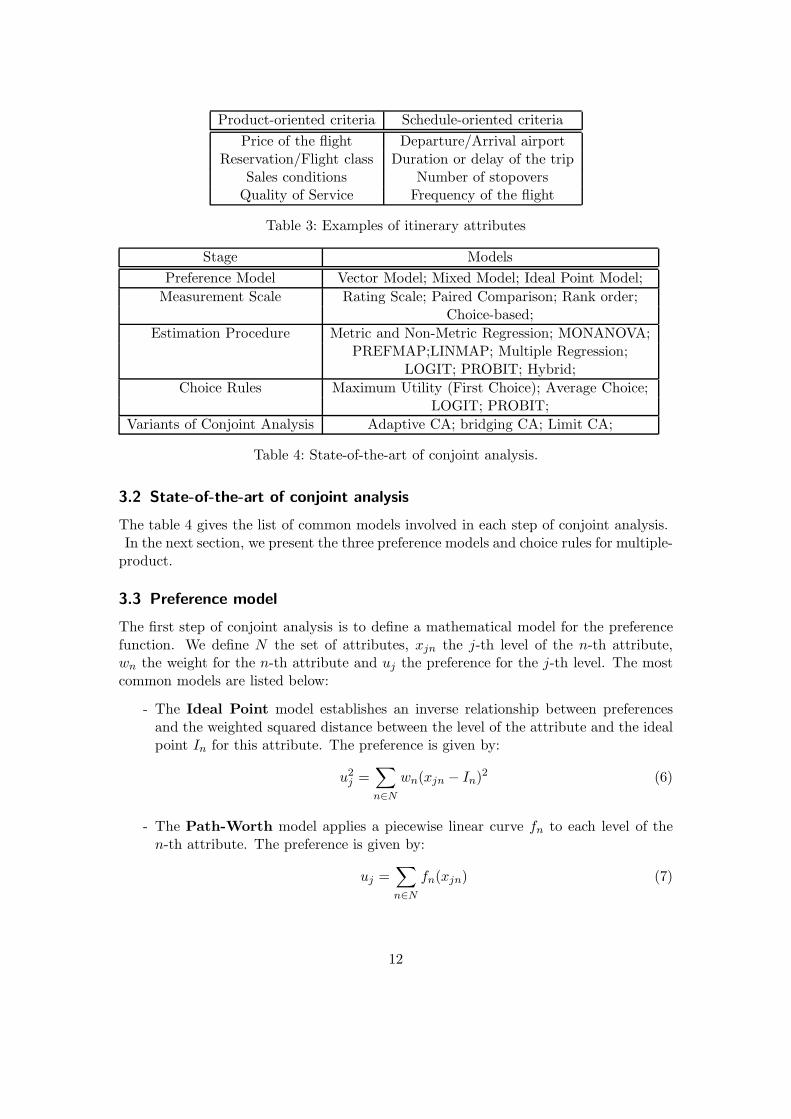
Stage Models

Preference Model Vector Model; Mixed Model; Ideal Point Model;

Measurement Scale Rating Scale; Paired Comparison; Rank order;Choice-based;

Estimation Procedure Metric and Non-Metric Regression; MONANOVA;PREFMAP;LINMAP; Multiple Regression;

LOGIT; PROBIT; Hybrid;

Choice Rules Maximum Utility (First Choice); Average Choice;LOGIT; PROBIT;

Variants of Conjoint Analysis Adaptive CA; bridging CA; Limit CA;

Table 4: State-of-the-art of conjoint analysis.

3.2 State-of-the-art of conjoint analysis

The table 4 gives the list of common models involved in each step of conjoint analysis.In the next section, we present the three preference models and choice rules for multiple-

product.

3.3 Preference model

The first step of conjoint analysis is to define a mathematical model for the preferencefunction. We define N the set of attributes, xjn the j-th level of the n-th attribute,wn the weight for the n-th attribute and uj the preference for the j-th level. The mostcommon models are listed below:

- The Ideal Point model establishes an inverse relationship between preferencesand the weighted squared distance between the level of the attribute and the idealpoint In for this attribute. The preference is given by:

u2j =

∑

n∈N

wn(xjn − In)2 (6)

- The Path-Worth model applies a piecewise linear curve fn to each level of then-th attribute. The preference is given by:

uj =∑

n∈N

fn(xjn) (7)

12

- The Vector model is represented by the weighted sum of all levels, where eachlevel of attribute is associated with an individual weight. The preference is givenby:

uj =∑

n∈N

wnxjn (8)

3.4 Choice rules

Choice rules allow to estimate the probability of choice from utility data. The threecommon models are described below:

- First Choice Rule Consumers select the product that maximizes their utility.The probability takes only the value 1 or 0, as shown in equation (9). Dobson G.,Kalish S.[12] use the first choice rule in their pricing subproblem to ensure thatcustomers select only the product with the highest utility.

pid =

1 when uid = maxi′∈I(ui′d)0 otherwise

(9)

where

pid : The probability that a customer d chooses the product i.uid : The utility of the d-th customer for the product i.I : The set of all the products, indexed with i.

- Bradley-Terry-Luce (BTL) or share of utility rule The probability to selecta product corresponds to the relative utility of the product, as shown in equation(10).

pid =uid

∑

i′∈I

ui′d

(10)

where

∑

i′∈I ui′d > 0,∀d ∈ D.

All preference values must be positive. Gaul W., Aust E., Baier D. [13] propose anew approach of the model with a probabilistic consumer behaviour model basedon the BTL model, called PROLIN. They extend the formulation of the BTLmodel by adding a market parameter α that allows a calibration of the model tothe market, as shown in equation (11).

pid =uα

id∑

i′∈I

uαi′d

(11)

where

α : The market parameter.

13

- Multinomial Logit (MNL) Rule The LOGIT model uses an assigned choiceprobability that is proportional to an increasing monotonic function of the alter-native’s utility. The probability that a consumer chooses a product is given bydividing the contribution of one product by the contribution of all other productsin the same way as the BTL model, as described in equation (12). Negative utilitiesare possible.

pid =exp(uid)

∑

i′∈I

exp(ui′d)(12)

Our integrated model will include a Multinomial Logit model as choice rule.

For the First-Choice model, market share is the number of trials with highest utilitydivided by all the trials. For the BTL and MNL model, market share is the arithmeticalmean of individual probabilities.There are, among others, two contributions in the conjoint-based product line designliterature: Green, Krieger [14] and Kohli, Sukumar [19]. We base our approach on bothapproaches. The fundamental difference between both formulations is that decisions aremade at different level. Green, Krieger decisions are made at the attribute level andKohli, Sukumar decisions at the product level. By analogy, we will differentiate twoformulations of our model as well: one at the itinerary level (product level) and theother at the attribute level. We discuss the formulation of the passenger preference atthe itinerary attribute level in section 4.2.2 and the one at the attribute level in section4.2.3.

4 Integrated model for airline schedule generation and product

line design

In this section, we introduce the framework of our work before we formulate our model.We detail the interaction between airline passengers demands and airline supply. Finallywe gave three formulations of our model. Notations are given at the end of the thesis.

4.1 Assumptions

An airline company seeks to integrate a set of markets, composed by a set of airports.Each OD-pair (couple of source airport and destination airport) defines a market. Forexample, Paris-Berlin is a market and Berlin-Paris is another market, and both arecalled opposite markets. Each OD-pair can be flown by a set of itineraries. An itineraryis a sequence of flight legs, that are characterized by an airport-source, an airport-destination, a departure time and an arrival time. Itineraries are products that theairline company wants to offer in a market. For the purpose of conjoint analysis, eachproduct is described by a set of attributes whose level set will be decided by the managersof the marketing’s department. Each flight can be direct (without stops) or with one ormore stopovers. Flights with stopovers are called via flights.

14

Figure 2: Incremental approach with base and master flight list.

4.1.1 Mandatory and Optional flight legs

Planners want to construct a schedule, which is basically a list of itineraries. In theincremental approach, they build it from a base schedule. The base schedule is modifieduntil the best schedule is found. At each iteration, the model takes as input a masterflight list, that is composed by mandatory flight legs and optional flight legs. Mandatoryflights have to be included in the final schedule while optional flights do not necessaryhave to. The modifications are the deletion or addition of flight legs. The output is a listof flight legs that maximizes the airline profit. An iteration of the schedule generationprocess is modelled in figure 2.

The final list of flight legs does not have to be a list of rotations (itineraries that startand end at the same airport). We do not restrict our approach to a daily schedule ora schedule that will be repeated. Our model is designed for an airline company, thatdesires to optimize a subset of their actual schedule by introducing new flights or deletingnon-profitable flights. In this case, itineraries are not rotations.

4.1.2 Airline Passenger Demand

Demand for air travel is indeed a derived demand. It is derived from other needs ofpassengers. People rarely fly from cities to cities for the mere sake of travelling on aplane. Airline passenger demand follows the standard assumptions of a product linedesign problem, namely,

15

(1) Each market is composed of different customer segments of various size. In ourthesis, we similarly talk about passenger segment or passenger d. Each segment d

of the demand represents a subset of passengers that follows the same consumerbehaviour. An example of segment could be students between 20 and 24 years old.In each customer segment, the unconstrained demand is the maximal number ofpassengers that the airline can capture.

(2) Airline passengers choose the flight, that provides the maximum utility. They cannot buy two tickets of one flight.

Each passenger preference will be determined during the conjoint analysis stage. Whenthe capacity of the aircraft is too small with regard to demand, passenger requests arerejected and the company loses the opportunity to increase its profit. This phenomenonis referred to as spill. But the company can cope with the spill by offering alterna-tive flights to the original offer, a flight with a stopover instead of a direct flight forexample. Our model takes the spill-recapture phenomenon into account by controllingdemand/passenger choice among available alternatives indirectly through pricing andfare product selection.

4.1.3 Airline Supply

Airlines commonly use a network structure to develop their supply strategy. As exposedin section 2.1.3, the structure underlying our model is a time line or time-space network.The figure 3 displays an example of a time line network for an aircraft type with threeairports and four time points.Nodes represent activities of aircraft type, in an airport and at a time t. Arcs represent

the movement of aircraft either in the air or on the ground. The network defines theairline company’s market. It describes all crucial information to ensure the feasibility of aschedule: input/output flights at each node, ground arcs, number of flights by OD-pairsand number of aircrafts in the air.

4.1.4 Fleet Assignment

The firm owns a finite fleet of different aircrafts or aircraft types. Each aircraft type hasspecial characteristics, such as the number of seats or the minimum ground time. Weassume that all aircrafts are available. The airline company can not assign more aircraftcapacity to flight legs than the available. Every mandatory flight has to be assigned anaircraft, while some optional flights not. To fulfill operational constraints mentioned insection 2.1.3, the fleet assignment stage takes the time line network as input. Figure 4displays an unfeasible schedule based on the simple time line network, shown in figure3. Each colour represents an aircraft.

In figure 4, the flow conservation constraint is not fulfilled at the node ”Paris 15 : 30”.The ”red” aircraft disappears after the node ”Paris 15 : 30”. The aircraft has to goeither to the node ”Paris 15 : 55” or to ”Boston 15 : 55”. The aircraft either has to

16

Figure 3: Time Line Network for an aircraft type.

Figure 4: Unfeasible schedule based on the Time Line Network figure 3.

17

Figure 5: Feasible schedule based on the Time Line Network figure 3.

stay in the same airport (ground arc) or fly to another airport (normal arc). Figure 5shows the feasible solution, where the aircraft stays at Paris airport between 15 : 30 and15 : 55.

The assignment cost vary depending on the flight legs flown and the aircraft type used.It represents the main cost in our model.

4.1.5 Competitive flights

A consumer can also be attracted by a competitive flight. Our model takes the competi-tion into account. Customers generally choose the best flight among all possible options:flights offered by the same airline company to another booking class non the same flightor to a low cost flights from other airlines. That is the reason why we model choicebehaviour that accounts for competitive flight legs.

4.2 Interaction between passenger demand and airline supply

As mentioned in the introduction, we base our approach of airline schedule design onthe integrated model of Lohatepannont M. and Barnhart C. [4], where the flow of airlinepassengers is determined by the passenger mix model. Our model adjusts the price ofitinerary considering the consumer preference. In the next subsection, we introduce thepassenger mix model and compare it to our model.

18

4.2.1 Passenger Mix Model

Given a fleeted schedule and the unconstrained itinerary demands, the Passenger MixModel finds the flow of passengers that maximizes the airlines profit. The formulationis given by:

Max∑

m∈M

∑

m′∈M

faremxmm′ (13)

∑

m∈M

∑

m′∈M

δmfxmm′ ≤ CAPf ∀f ∈ Ω (14)

∑

m′∈M

xmm′

bmm′

≤ Dm ∀m ∈ M (15)

xmm′ ≥ 0 ∀m,m′ ∈ M (16)

where variables are:

xmm′ : the number of passengers who fly on itinerary m that desire to travel onitinerary m′.

farem : the average fare of itinerary m.CAPf : the capacity of flight f .bmm′ : the recovery rate of passengers desiring itinerary m who are offered itinerary m′.δmf : equals 1 if flight f covers itinerary m and 0 otherwise.Dm : unconstrained demand on itinerary m.

Constraints (14) are the capacity constraints that ensure that the number of passengerson a flight does not exceed the number of seats available. Constraints (15) are the de-mand constraints ensuring that the total number of passengers that is accommodatedor spilled does not exceed the corresponding unconstrained demand.Our approach is to express xmm′ with consumer preferences and to consider a pricingproblem. The number of passengers who fly on one itinerary is now the result of theproduct between the probability that passengers select this itinerary and the uncon-strained demand for the corresponding itinerary. Hence, the demand constraints are notneeded anymore because the fraction of passengers on a flight is now always inferior tothe unconstrained demand . The probability that passengers choose an itinerary is afunction influenced by the price. The price is modelled as a continuous decision variable.With our notations and the assumption of a demand segmentation, we formulate themodel as the adjustment of prices that maximizes the profit:

Max∑

m∈M

∑

d∈demm

farempdmωd (17)

∑

m∈M

∑

d∈demm

δfmpdmωd ≤ CAPf ∀f ∈ Ω (18)

0 ≤ pdm ≤ 1 (19)

19

farem ≥ 0 (20)

The probability pdm that a passenger decides to fly the itinerary m as a function of priceand other fare product attributes will be the subject of sections 4.2.2 and 4.2.3. Wehave modelled the preference measurement with the methods of conjoint analysis. Weobserved two approaches, by comparison to the formulations of Green, Krieger and theone of Kohli, Sukumar [14]:

(1) Conjoint analysis with decisions at the itinerary attribute level.

(2) Conjoint analysis with decisions at itinerary level.

We discuss advantages and disadvantages of each approach in the next two sections.

4.2.2 Conjoint analysis at the itinerary attribute level

Each itinerary is described by a finite set of attributes. Prior to the schedule generationstage, the marketing’s department conducts the analysis that gives the utility of thepassenger d for the assignment of j-th level to the n-th attribute. The probability that apassenger selects an itinerary for a BTL model is given by equation (21) and for a MNLmodel by equation (22):

pdm =

N1∑

n=1

Jn∑

j=1

xjnmudjn

|M |+|Mc|∑

m1=1

(

N1∑

n=1

Jn∑

j=1

xjnm1udjn)

(21)

pdm =

exp(

N1∑

m=1

Jn∑

j=1

xjnmudjn)

|M |+|Mc|∑

m1=1

(exp(

N1∑

n=1

Jn∑

j=1

xjnm1udjn))

(22)

where:

N1 : Set of attributes of an itinerary, indexed by n.Jn : Set of level sets for the attribute n, indexed by j.xjnm : = 1, when the n-th attribute is assigned to the j-th level in the itinerary m, = 0

otherwise. These are binary constants for m ∈ M c (competitive itineraries) andbinary decision variables for m ∈ M .

udjn : Utility of the passenger d for the assignment of j-th level set to the n-th attribute.Utilities can be negative in a MNL model.

The choice of a consumer for an itinerary is considered only if the itinerary is includedin the master flight list. Hence, the probability pdm should be equal to zero when the

20

itinerary is not served (qm = 0).

In equations (21) and (22), we should differentiate the price from the other attributes,because decisions on prices yield revenue. In our model, we consider price as first at-tribute, indexed with 0 (n = 0). Marketers select the price of an itinerary among a setof possible prices. The choice of charging a passenger with a price level for an itineraryinfluences the passenger preference for this itinerary. The assignment of the j-th pricelevel to an itinerary has an utility udj0, given by conjoint analysis. The choice of itineraryprices directly intervenes in the objective function. The price of an itinerary m is shownin equation (23).

J0∑

j=1

xj0mfarejm ∀m ∈ M (23)

where

J0 : Set of possible prices, indexed by l.xj0m : =1, when a passenger is charged with the j-th possible price for itinerary m.farejm : j-th level of the price for the itinerary m.

With the contribution of the price, the probability that a consumer selects an itinerarybecomes (24) for the BTL model and (25) for the MNL model.

pdm =

N∑

n=0

Jn∑

j=1

xjnmudjnqm

|M |∑

m1=1

N∑

n=0

Jn∑

j=1

xjnm1udjnqm1

+

|Mc|∑

m1=|M |+1

N∑

n=0

Jn∑

j=1

x′jnm1

udjn

(24)

pdm =

exp(

N∑

n=0

Jn∑

j=1

xjnmudjn)qm

|M |∑

m1=1

exp(

N∑

n=0

Jn∑

j=1

xjnm1udjn)qm1

+

|Mc|∑

m1=|M |+1

exp(

N∑

n=0

Jn∑

j=1

x′jnm1

udjn)

(25)

where

N : Set of attributes of an itinerary, with the price as first attribute and the otherattributes are service-oriented.

xjnm1are decision variables.

x′jnm1

are binary constant.

qm : =1 when itinerary m is included in the schedule, = 0 otherwise.

In product line design, decision makers must assign exactly one level to each attributeif the product is offered. Furthermore, each product should have all attributes assigned,in order to be introduced in a market. As itineraries are products in our model, every

21

itinerary included in the schedule has to fulfill both constraints. Condition (26) ensuresthat each attribute of an itinerary/fare product is assigned at most one attribute levelonce.

Jn∑

j=1

xjnm ≤ qm ∀n ∈ N,∀m ∈ M (26)

To be included in the master flight schedule, each itinerary should have all attributesassigned. Equation (27) guarantees this requirement.

Jn∑

j=1

xjnm =

Jn+1∑

j=1

xj(n+1)m ∀n ∈ N,∀m ∈ M (27)

We cast both requirements in equation (28).

Jn∑

j=1

xjnm = qm ∀n ∈ N,∀m ∈ M (28)

This approach considers the assignment of a level to an attribute (xjnm) as decisionvariables, with price as first attribute and other schedule-oriented attributes. The firstdisadvantage of this approach is the large number of decision variables. The measurementof the utility for each attribute and the determination of decision variables could becomputationally challenging. If there are 10 passenger segments, 10 attributes with 10levels, then there are 10.1010 utilities to measure and |M | ∗ 10 ∗ 10 decision variablesper itinerary are to be determined. Furthermore the relationship between the choice ofitinerary prices and the passenger behaviour is not accurate because of the restrictionof the prices to a finite set of possible values. That is why we propose an approach at ahigher level where prices are continuous decision variables.

4.2.3 Conjoint analysis at the itinerary level

At the itinerary level, utilities are associated with itineraries, instead of itinerary at-tributes. Utility as monetary value represents the price that a customer is willing to payfor an itinerary. We assume here that these values are not influenced by the price but areindeed schedule-oriented or related to the quality of service. We suppose that utilitieshave been determined by conjoint analysis before schedule’s operation. Decision makerschoose price and select which itineraries as combination of non-price attribute levels tooffer. Itineraries as combinations of non-price attributes are defined exogenously priorto the decision making process considered here and can be regarded as input to theoptimization model. Prices are continuous variables in this approach.The expression of the probability that a customer chooses an itinerary is given by (29)for a BTL model and (30) for a MNL model:

pdm =max(Udm − farem, 0)qm

|M |∑

m′=1

max(Udm′ − farem′ , 0)qm′ + Ud0

(29)

22

pdm =e(Udm−farem)qm

|M |∑

m′=1

e(Udm′−fare

m′ )qm′ + Ud0

(30)

where

Ud0 : Given utility of passenger segment d for competitive itineraries.farem : Price of the itinerary m.

Passengers preferences are driven by the fare of itineraries. Since prices are continuousvariables, the expression Udm − farem can take negative values when the price chargedby the airline company exceeds the price expected by the consumer. But a BTL modelis defined for positive utilities only. That is why the probability that a customer selectsan itinerary is equal to zero, when the price is bigger than the utility (farem ≫ Udm)in the BTL model (max(Udm − farem, 0) in equation 29). As far as the MNL modelis concerned, the passenger preference is close to zero, when the price is bigger thanthe utility. The influence of the price on the customer’s behaviour is more accurate atitinerary level than at itinerary attribute level. We choose to integrate the MNL modelas choice rule.

We suggested that this method considers the passenger choice model from a higherlevel. The relationship between the utility at itinerary attribute level and at itinerarylevel is given by:

Udm =

N∑

n=0

Jn∑

j=1

xjnmudjn (31)

Ud0 =

|Mc|∑

m1=|M |+1

N∑

n=0

Jn∑

j=1

x′jnm1

udjn (32)

Thus (24) can be deduced from (29).We decided to implement the product line design model at the itinerary level, becauseprices are represented as continuous variables and passenger behaviours are more sensi-tive to prices in this approach.

4.3 Objective Function

Our problem maximizes the airline profit considering assignment costs and passengercosts. The objective function is composed by the following components:

- The profit gained from the price of tickets. The total profit R is given by (33) fordiscrete prices and (34) for continuous prices:

R =∑

m∈M

∑

d∈demm

J0∑

j=1

xj0mfarejmpdmωd (33)

R =∑

m∈M

∑

d∈demm

farempdmωd (34)

23

- The total cost for assigning fleets to flight legs:

C1 =∑

f∈Ω

∑

k∈K

cfkθfk (35)

- The total cost for carrying passengers:

C2 =∑

m∈M

∑

d∈demm

cmpdmωd (36)

- Maximizing the profit and minimizing the costs the objective function becomes:

Max(R − C1 − C2) (37)

4.4 Formulations

We give in this section three formulations of our integrated model. The first two formula-tions differentiate the two approaches of the consumer preference. The third formulationis the special case where we do not consider the demand segmentation. This last sim-plification was decided for implementation’s purpose.

4.4.1 Formulation with utility at itinerary attribute level

max(∑

m∈M

∑

d∈demm

(

J0∑

j=1

xj0mfarejm − cm)pdmωd −∑

f∈Ω

∑

k∈K

cfkθfk) (38)

subject to∑

m∈M

∑

d∈demm

δfmpdmωd ≤∑

k∈K

capkθfk ∀f ∈ Ω (39)

pdm =

exp(

N∑

n=0

Jn∑

j=1

xjnmudjn)qm

|M |∑

m1=1

exp(N

∑

n=0

Jn∑

j=1

xjnm1udjn)qm1

+

|Mc|∑

m1=|M |+1

exp(N

∑

n=0

Jn∑

j=1

x′jnm1

udjn)

(40)

∑

f∈I(k,a,t)

θfk + zk,a,t− −∑

f∈O(k,a,t)

θfk − zk,a,t+ = 0 ∀k, a, t ∈ P (41)

∑

a∈A

zk,a,t +∑

f∈Ωk

θfk ≤ Nk ∀k ∈ K (42)

qm −∑

k∈K

θfk ≤ 0 ∀f ∈ Ωm,∀m ∈ M (43)

24

qm −∑

f∈Ωm

∑

k∈K

θfk ≥ 1 − Nm ∀m ∈ MO (44)

∑

k∈K

θfk ≤ 1 ∀f ∈ ΩO (45)

∑

k∈K

θfk = 1 ∀f ∈ ΩM (46)

Jn∑

j=1

xjnm = qm ∀n ∈ N,∀m ∈ M (47)

zk,a,t ≥ 0 ∀k, a, t ∈ P (48)

θfk binary ∀f ∈ Ω,∀k ∈ K (49)

xjnm binary ∀j ∈ Jn,∀n ∈ N,∀m ∈ M (50)

qm binary ∀m ∈ M (51)

Constraints (39) ensure that the available capacity of the aircraft limits the constrainingdemand. Constraints (40) are related to the preference measurement calculated in (24)with a MNL model. Constraints (41) and (42) are fleet assignment constraints. Theflow conservation constraint for aircraft routings is given by (41). The optimal solutionfulfills the classical plane count constraint given by (42). The sum of aircrafts of onetype in the air and on the ground are limited by the fleet size of this aircraft type ateach time.Constraints (43) and (44) are itinerary status constraints. Constraints (43) ensure thataircraft capacity is assigned to all flights included in the schedule. Constraint (44)ensures that an itinerary m is included if all of its flight legs are flown. Constraints (45)and (46) are cover constraints. They ensure that at most one aircraft is assigned to aoptional/mandatory flight. Constraints (47) are related to product line design problemand pricing. They guarantee that if an itinerary is included in the schedule, all attributesof this itinerary are assigned to a level.

4.4.2 Formulation with utility at the itinerary level

max(∑

m∈M

∑

d∈demm

(farem − cm)pdmωd −∑

f∈Ω

∑

k∈K

cfkθfk) (52)

subject to∑

m∈M

∑

d∈demm

δfmpdmωd ≤∑

k∈K


pdm =e(Udm−farem)qm

|M |∑

m′=1

e(Udm′−fare

m′ )qm′ + Ud0

∀d ∈ demm,∀m ∈ M (54)

25

∑

f∈I(k,a,t)


f∈O(k,a,t)

θfk − zk,a,t+ = 0 ∀k, a, t ∈ P (55)

∑

a∈A

zk,a,t +∑

f∈Ωk

θfk ≤ Nk ∀k ∈ K (56)

qm −∑

k∈K

θfk ≤ 0 ∀f ∈ Ωm,∀m ∈ M (57)

qm −∑

f∈Ωm

∑

k∈K

θfk ≥ 1 − Nm ∀m ∈ MO (58)

farem ≤∑

f∈Ωm

faref ∀m ∈ M (59)

∑

k∈K

θfk = 1 ∀f ∈ ΩM (60)

∑

k∈K

θfk ≤ 1 ∀f ∈ ΩO (61)

zk,a,t ∈ N ∀k, a, t ∈ P (62)

farem ≥ 0 ∀m ∈ M (63)



Schedule generation and fleet assignment constraints are the same as the first formu-lation. The preference in (54) is modelled at the itinerary level with a MNL model.Constraints (59) guarantee that a via flight is not more expensive than the sum of itsflight legs. We do not use separate variables for the price of an itinerary (farem) andthe price of a flight leg (faref ) considering that flight legs are fleeted itineraries reducedto a flight arc in the network.

4.4.3 Formulation with utility at the itinerary level without demand segmentation

max(∑

m∈M

(farem − cm)pmωm −∑

f∈Ω

∑

k∈K

cfkθfk) (66)

subject to∑

m∈M

δfmpmωm ≤∑

k∈K


pm =e(Um−farem)qm

|M |∑

m′=1

e(Um′−fare

m′ )qm′ + U0

∀m ∈ M (68)

26

∑

f∈I(k,a,t)


f∈O(k,a,t)

θfk − zk,a,t+ = 0 ∀k, a, t ∈ P (69)

∑

a∈A

zk,a,t +∑

f∈Ωk

θfk ≤ Nk ∀k ∈ K (70)

qm −∑

k∈K

θfk ≤ 0 ∀f ∈ Ωm,∀m ∈ M (71)

qm −∑

f∈Ωm

∑

k∈K

θfk ≥ 1 − Nm ∀m ∈ MO (72)

farem ≤∑

f∈Ωm


∑

k∈K

θfk = 1 ∀f ∈ ΩM (74)

∑

k∈K

θfk ≤ 1 ∀f ∈ ΩO (75)

zk,a,t ∈ N ∀k, a, t ∈ P (76)

farem ≥ 0 ∀m ∈ M (77)



The variables Udm, pdm and ωd have become independent of the demand segment d. Allconstraints stay the same.

5 Solution Approaches

As for the solution approaches, we consider the formulation with utility at the itinerarylevel, exposed in 4.4.2.

5.1 Problem class

The first observation is that our model is not linear because of the choice model lead-ing to nonlinear objective function (54) and nonlinear capacity constraint (55). Ourmodel has continuous decision variables (farem) and integer decision variables (zk,a,t,θfk and qm). Our model belongs then to the Mixed Integer nonlinear Programming class.

Classical methods decompose the problem by separating the nonlinear part from theinteger part. A Branch-and-Bound algorithm performs a tree-search and solves a nonlin-ear problem (NLP) at each node. We have chosen this implementation because optimiza-tion software packages (Numerical Algorithms Group Library) are available to solve thenonlinear part with Sequential Quadratic Programming (SQP) methods. We integrate

27

this SQP methods into our own implementation of the Branch-and-Bound algorithm.

We acknowledge that a better way could have been an integrated algorithm as realizedby Leyffer [20]. Leyffer proposes an algorithm where the tree search and the iterativesolution of the nonlinear problem are interlaced. Thus, the nonlinear part is solvedwhilst searching the tree. The underlying idea is to branch before an iteration of theSequential Quadratic Programming (SQP) solver.The section 5.2 introduces the two methods Branch-and-Bound and Sequential QuadraticProgramming.

5.2 Branch-and-Bound

The solution space of an integer programming problem can be assumed finite. Thesimplest way to solve the integer problem is to go through all integer points, discardinginfeasible ones and always keeping track of the feasible solution with the best objectivevalue. The Branch and Bound considers a continuous problem defined by relaxing theinteger restrictions on the variables (θfk and qm in our model). Therefore, the solutionspace of the integer problem is only a subset of the continuous problem. If the optimalcontinuous solution is all integer, then it is also optimal for the integer problem. TheBranching operation partitions the continuous solution space into subspaces, which arealso continuous. The purpose of the partitioning is to eliminate points that are notfeasible for the integer problem. The Bounding operation helps locating the optimumsolution by comparing the objective function value of the current node to the objectivefunction value of the current best feasible solution (this upper bound is set to infiniteuntil a feasible solution is found). The optimum integer solution is available when thesubproblem having the greatest upper bound (considering a maximization problem)among all subproblems yields an integer solution. The tree to explore could have avery large number of branches and nodes. Branch-And-Bound algorithms may requirelarge computer storage since each node has an associated subproblem whose solutionand objective function must be stored. The Branch-and-Bound method proceeds asfollowed: First, the integer problem is replaced by a continuous space by relaxing theinteger conditions. Then branching is used to eliminate parts of the continuous one thatare not feasible by reactivating some of the integer restrictions. The process operatesbranching and bounding until all integer points have been tried. Branch-and-Boundalgorithms grow exponentially with the problem size but are exact solution methods.

5.3 Sequential Quadratic Programming methods

Sequential Quadratic Programming (SQP) methods solve an nonlinear problem via asequence of quadratic programming (QP) approximations obtained by replacing thenonlinear constraints by a linear first order Taylor series approximation and the nonlinearobjective by second order Taylor series approximation augmented by a second orderinformation from the constraints. They can converge quadratically near a solution. Butthey can fail to converge if they start far from a local solution. To ensure convergence,

28

each iteration of the SQP must decrease a penalty function, which is a linear combinationof the objective function and some measures of the constraint violation.

5.4 Incremental airline schedule model

The solution approach with Branch-and-Bound and SQP methods can not ensure tofind the optimum solution. The convergence of the SQP function relies on the choiceof the feasible starting point. That is the reason why an incremental approach fits ourproblem. As shown in the flow chart of figure 6, we start with a base schedule thatwe incrementally improve. If the stopping criteria is not met (for example, insufficientimprovement of the objective function), non-profitable itineraries can be identified, abetter starting point can be chosen and the heuristic can be started again. This methodallows to improve the starting point, until the objective function can not be improvedfurther. But the determination of non-profitable itineraries is uneasy. Therefore is thisstage manually operated.Branch-and-Bound combined with SQP is not the only way to solve the problem. Otherheuristics are possible such as Greedy algorithm, Nearest Neighbour algorithm or geneticalgorithm.

6 Implementation

6.1 Framework

We have implemented an Branch-and-Bound algorithm with a sequential QP method ateach node to solve the third formulation of our problem. We discuss in this section thekey point of the implementation. The algorithms are implemented in the C language.We used a function of the Numerical Algorithms Group’s Library to realize the SQPmethods, briefly described in section 6.2. And we have implemented our own Branch-and-Bound with different search strategies.

6.2 Numerical Algorithms Group library (eu04cc)

The function nag opt nlp of the package eu04cc allows to solve a problem with non-linearconstraints using a sequential quadratic programming (SQP) method. It takes as input:the number of decision variables n, the number of linear constraints nclin, the numberof nonlinear constraints ncnlin upper and lower bound for each variable bl and bu,matrix of coefficients of linear constraints a, functions that calculate the first derivativeof the objective function objfun and nonlinear constraints confun, the current objectivefunction objf and the associated first derivatives objgrd and a feasible starting point x.The declaration of the function is displayed below.

e04ucc(n, nclin, ncnlin,&a[0][0], tda, bl, bu,

objfun, confun, x,&objf, objgrd,

E04 DEFAULT,NAGCOMM NULL,NAGERR DEFAULT );

29

Figure 6: Flow Chart for incremental solution.

30

We also have to calculate the partial derivative of the non-linear constraints and theobjective function with respect to all the variables as input. The derivatives allow tocalculate the first and second order Taylor series approximation for nonlinear constraintsand the objective function. They are written in the functions confun and objfun

respectively, declared as:

staticvoidNAG CALLobjfun(Integern, doublex[], double ∗ objf,

doubleobjgrd[], Nag Comm ∗ comm)

staticvoidNAG CALLconfun(Integern, Integerncnlin, Integerneedc[],

doublex[], doubleconf [], doubleconjac[],

Nag Comm ∗ comm)

The Nag function solves only a minimization problem, while our problem is a maximiza-tion problem. Thus, we have to transform our problem into a minimization problem:

min(∑

f∈Ω

∑

k∈K

cfkθfk −∑

m∈M

(farem − cm)pmωm) (80)

subject to∑

m∈M

δfmpmωm ≤∑

k∈K


pm =e(Um−farem)qm

|M |∑

m′=1

e(Um′−fare

m′ )qm′ + U0

∀m ∈ M (82)

∑

f∈I(k,a,t)


f∈O(k,a,t)

θfk − zk,a,t+ = 0 ∀k, a, t ∈ P (83)

∑

a∈A

zk,a,t +∑

f∈Ωk

θfk ≤ Nk ∀k ∈ K (84)

qm −∑

k∈K

θfk ≤ 0 ∀f ∈ Ωm,∀m ∈ M (85)

qm −∑

f∈Ωm

∑

k∈K

θfk ≥ 1 − Nm ∀m ∈ MO (86)

farem ≤∑

f∈Ωm


∑

k∈K

θfk = 1 ∀f ∈ ΩM (88)

31

∑

k∈K

θfk ≤ 1 ∀f ∈ ΩO (89)

zk,a,t ∈ N ∀k, a, t ∈ P (90)

farem ≥ 0 ∀m ∈ M (91)

θfk, qm ∈ [0, 1] ∀f ∈ Ω,∀k ∈ K,∀m ∈ M (92)

The partial derivative of the objective function (f) and the nonlinear constraints (c1)are given in the appendix, at the end of the thesis.

In our solution, we differentiate two calls of the SQP functions, depending on the num-ber of decision variables. At the very beginning, we employ the SQP methods to findthe root of the Branch-and-Bound algorithm. All the variables are relaxed, qm and θfk

changed into continuous decision variables between 0 and 1, instead of binary variables,as shown in the constraints 92. The Branch-and-Bound algorithm will branch on thevalues of qm and θfk, that are not set 0 or 1. The algorithm goes through all the possiblecombinations of qm and θfk. At each node of the search tree, we operate another call ofthe SQP function, where qm and θfk are not variables anymore.

The starting point of the SQP methods is randomly chosen. In practice, we havemanually tried different points until we find a point that converges to an optimum.Once we have found a relative good starting point, we start the Branch-and-Boundalgorithm. At each node, we solve the same problem but the two binary variables qm

and θfk are now fixed by the branching strategy. The problem is given by:

min(∑

f∈Ω

∑

k∈K

cfkθfk −∑

m∈M

(farem − cm)pmωm) (93)

∑

m∈M

δfmpmωm ≤∑

k∈K


pm =e(Um−farem)qm

|M |∑

m′=1

e(Um′−fare

m′ )qm′ + U0

∀m ∈ M (95)

∑

f∈I(k,a,t)

θfk + zk,a,t+ −∑

f∈O(k,a,t)

θfk − zk,a,t− = 0 ∀k, a, t ∈ P (96)

∑

a∈A

zk,a,t +∑

f∈Ωk

θfk ≤ Nk ∀k ∈ K (97)

farem ≤∑

f∈Ωm


zk,a,t ∈ N ∀k, a, t ∈ P (99)

farem ≥ 0 ∀m ∈ M (100)

In this case, the formulas of the first derivative are the same as before. But the onlydecision variables are now farem and zk,a,t and all the others are parameters.

32

CreateQueue(Q) /*Q queue with priority: each element is a couple (Node,Estimation) */A = a feasible solution for the first SQP iterationRoot=SQP1(A) /* first call of the SQP function */Z=RootPush(F,(Z,f(Root)))ubound=infiniteWhile Not is Empty(F)

Pop(F,Z)x = Last Node of ZIf x is not a feasible solution

y1, ..., yk successors of x that don’t belong to ZFor i = 1 to k

A’=Z + yi /*Branching*/T=SQP2(A’) /* Second call of SQP function*/Push(F,(T,f(yi)))

End ForElse

if estimation value ≤ uboundubound = estimation value

End Iffathom

End IfEnd While

Figure 7: Formal description of the basic Branch-And-Bound algorithm

6.3 Branch-and-Bound algorithm

6.3.1 Formal description

Branch-and-Bound algorithms allow to reduce the ”solution space”. Each node is eval-uated regarding to an estimation function f, which is the value of the objective functionafter applying the SQP method. An upper bound, that represents the objective functionvalue of the best feasible solution, is chosen beforehand to decide whether a node will befathomed or not. It is fixed to infinite at the beginning. The tree search goes on until allinteger points have been tried. The basic formal Branch-and-Bound algorithm appliedto our problem is given in figure 7.

6.3.2 Improving Branch-and-Bound through search strategy

A way to improve the efficiency of the Branch-and-Bound method is to find a feasiblesolution as fast as possible and then allow to reduce the solution space by fathomingwith a small upper bound. To do so, we combine two different tree-search strategies:

33

Figure 8: Branch-and-Bound with Best first search.

Best First strategy and depth first search strategy. Our Branch-and-Bound algorithmperforms first a Depth First search until it finds a feasible solution then it switches tothe Best First strategy allowing a faster reduction of the space solution. In figure 9, ourcombined algorithm is applied, while a Best First strategy is applied figure 8. The DepthFirst strategy found a relative bad feasible solution (objective function value = −970)compared to the Best First strategy (objective function value = −992). But the upperbound was found faster than the Best First strategy, 2 iterations against 3 iterations.This difference in iterations is already important, given that the example has only 4leaves.The difference between the two search strategies depends on how the queue is prioritized.

The queue is realized as an ordered list by decreasing estimation values for the best firststrategy and ordered by depth in the search tree for the depth first strategy. We namethe functions, that add a new element to the stack, for each search strategy bPUSH

and dPUSH and the function, that takes the best element according to the objectivefunction (for the best first strategy) or the depth (for the depth first strategy) off thestack, POP . The POP function stays the same in both cases, since the best solutionis always on top of the stack. The Branch-and-Bound algorithm with combined searchstrategies is shown in figure 10.The Branch-and-Bound algorithms are exact solution methods but they can still explore

a large set of nodes. In practice, we implement a truncated Branch-and-Bound for largescale problems. In section 7.6, we discuss a stopping criteria that determines when areasonable feasible solution is found.

34

Figure 9: Combination of Best first and Depth first tree search.

7 Computational Results

In this section, we present the performance analysis that we have conducted to test ourimplementation. The intention is to provide some insights about the solvability of ourapproach. Since it is difficult if not impossible to prove whether the algorithm reachesthe optimum or not for a large nonlinear problem, we use small time line networks toreduce the complexity of the problem. We start with a schedule with only one flight leg.We study the influence of the passenger preference to the optimum schedule. At theend, we present and discuss the results of our algorithm for a problem with 5 OD Pairs.The time line networks are based on data from European airline websites. The utilityvalues, assignment costs, passenger costs and aircraft capacities are randomly fixed.

7.1 Problem with 1 OD-Pair

First, we consider the problem reduced to one OD-pair, one flight leg and the parametersshown in table 5. We consider that the airline only owns two aircrafts. The optimumis the maximum of the following objective function subject to operational constraints(67)-(79).

max((fare − c)e(U−fare)qω

e(U−fare)q + U0− (c00θ00 + c01θ01)) (101)

We note that is already difficult to find the optimum of the problem. In this particularcase, the SQP function converges 98% of the cases to the same convergence point with aprofit of 131, 021721. Even though all variables are relaxed, all binary decision variablesare 0 or 1. The convergence is sensitive to the choice of the starting point. The table 6

35

CreateQueue(Q)A = feasiblesolutionfor the first SQP iterationRoot=SQP1(A) /* first call of the SQP function */Z=RootdPush(F,(Z,f(Root)))Found=FalseDepth = 0ubound=infiniteWhile Not isEmpty(F)

Pop(F,Z)x = Last Node of ZDepth=Depth+1If x is not a feasible solution

y1, ..., yk successors of x that don’t belong to ZFor i = 1 to k

A’=Z + yi /*Branching*/T=SQP2(A’) /* Second call of SQP function*/if Found

bPush(F,(T,f(yi)))else

lPush(F,(T,f(yi)),k)End If

End ForElse

if estimation value ≤ uboundubound = estimation value

End Ifif Found = False

order Q by estimation valueFound = True

End Iffathom

End IfEnd While

Figure 10: Formal description of the Branch-and-Bound algorithm with combined searchstrategies.

36

UTILITY Value

U0 20

U1 23

DEMAND FACTOR

ω0 20

ASSIGNMENT COST

costa00 10

costa01 20

PASSENGER COST

costm0 10

CAPACITY OF AIRCRAFT

cap0 50

cap1 40

Table 5: Numerical values of the parameters for the first example.

shows the initial point and the optimum.

7.2 Influence of the consumer preference on the optimum schedule

Our model gives an important part to the consumer preference. We are about to testhow consumer preference influences price. We choose a network with two OD-Pairs andone flight leg per OD pair, as shown in figure 11. Both flights are optional. Parametersare given in table 7.

We set up a flight leg with a low utility (U1 = 23) and another one with high utility(U2 = 40). The most preferred flight has a bigger cost per passenger than the other.With a starting schedule that includes only one flight leg, the SQP method always ends

up including the most preferred flight leg and excluding the other. In this case, somecalls of SQP converge to the same point with objective function 575.402129 and the flightf1 included in the final schedule, detailed in table 8. We try to build manually schedulesincluding only the flight f1 and with a price close to the optimum price (between 30and 40). Since the solution that we try to improve is a local maximum, we did not findbetter objective function value than 575.402129. We also try schedules that only includethe first flight leg (f0). The objective function does not exceed 40 and the solver oftenstops, because the first-order-Kuhn-Tucker constraints have failed.

This point is the best convergence point but we have found other convergence pointswith objective function value 555.402107, that include both flight legs in the optimumschedule. One of this local convergence point is displayed in table 10. If we increasethe price of the first flight leg, the convergence point stays the same with the new priceinstead. The contribution of the first flight does not yield profit to the airline, whenit is included. The probability that a passenger chooses the first flight is close to zero,because of the contribution of the second flight (the most preferred flight). The expo-

37

initial zk,a,t initial θfk initial farem initial qm initial objfun

z000 = 0 θ00 = 0 fare0 = 22 q0 = 1 8,716416

z001 = 0 θ01 = 1

z010 = 0

z011 = 0

z100 = 1

z101 = 0

z110 = 0

z111 = 1

final zk,a,t final θfk final farem final qm final objfun

z000 = 1 θ00 = 1 fare0 = 18.051086 q0 = 1 131,021721

z001 = 0 θ01 = 0

z010 = 0

z011 = 1

z100 = 0

z101 = 0

z110 = 0

z111 = 0

Table 6: Initial and final point for the first example

Figure 11: Example with 2 OD-Pairs.

38

UTILITY Value

U0 20

U1 23

U2 40

DEMAND FACTOR

ω0 20

ω1 18

ASSIGNMENT COST

costa00 10

costa01 20

costa10 10

costa11 20

PASSENGER COST

costm0 10

costm1 20


cap0 50

cap1 40

Table 7: Parameters for an airline network with 2 OD-Pairs

nentials in the preference intensify the difference between utilities. If the utility of themost preferred flight (f1) decreases of 10%, the optimum schedule will still include it andthe optimum price will be reduced of 29%. The probability that a passenger chooses f1

will only diminish of 2%. A small difference between utilities can imply great changesin the optimum schedule.

With the numerical parameters that we choose in this example with 2 OD-Pairs, it isalways more profitable to include only one flight leg in the schedule. Even if we startthe solver when flights have exactly the same assignment costs, same fare and sameutility, the SQP function will end up including only one flight with the maximum fare.Including the other flight leg introduce more costs than it yields revenue. In practice,if we keep the maximum fare for the second flight and try to add the first flight to theschedule, it converges to another convergence point.

If the starting point is too far from the optimum, the SQP function will not converge.After trying several starting points, we observe three outputs with the frequencies dis-played in table 12. The execution time is always less than 1 second. The SQP functiondid not converge in only 5% of times.

But these percentages do not accurately represent the reality, because the startingpoints of our test have not been generated by a random function and we did not tryall possible starting points. These percentages are correlated with the probability to

39


z000 = 1 θ00 = 0 fare0 = 22 q0 = 1 15.213931

z001 = 0 θ01 = 1 fare1 = 20 q1 = 0

z010 = 0 θ10 = 0

z011 = 1 θ11 = 0

z020 = 0

z021 = 0

z100 = 0

z101 = 0

z110 = 0

z111 = 0

z120 = 1

z121 = 1


z000 = 0 θ00 = 0 fare0 = 0 q0 = 0 575.402129

z001 = 0 θ01 = 0 fare1 = 33.522340 q1 = 1

z010 = 0 θ10 = 1

z011 = 1 θ11 = 0

z020 = 1

z021 = 0

z100 = 0

z101 = 0

z110 = 0

z111 = 0

z120 = 0

z121 = 0

Table 8: Initial and final point for the second example

Utility (optimum) Price Probability (f1)

40 33.522340 0.970169

35 28,683434 0.965137

30 23.874256 0.958114

27 19,107958 0.952399

Table 9: Influence of the utility to the flight f1

40


z000 = 1 θ00 = 0 fare0 = 37 q0 = 1 555.382006

z001 = 0 θ01 = 1 fare1 = 33.5700 q1 = 1

z010 = 0 θ10 = 1

z011 = 1 θ11 = 0

z020 = 0

z021 = 0

z100 = 0

z101 = 0

z110 = 0

z111 = 0

z120 = 1

z121 = 1

Table 10: Initial point with both flight legs included

generate a schedule with two flight legs (respectively with one flight leg).

This second test underlines two aspects of our approach:

(1) In our model prices and the probability of choosing a flight leg are sensitive to util-ities. Even a small difference in utility values can completely change the optimumschedule.

(2) The convergence of the SQP function depends on the distance between the startingpoint and the optimum point. The incremental approach allows to improve thestarting point at each iteration.

So far, the computational results have given contribution to the convergence of theSQP function and to the interaction between high passenger demand and airline supply.In the next section, we evaluate the performance of the complete algorithm (Branch-and-Bound and SQP function) for a larger problem.

7.3 Performance of the first call of the SQP function

We consider a set of five OD-pairs with only one flight per OD-pair, as shown in figure12, with the time line network in figure 13 and the parameters in table 14. There are onlytwo aircrafts, in order to keep the problem size small (80 variables and 95 constraints).Table 13 presents the size of the constraint matrix. Like the example with two flightlegs, we run the SQP function with all variables relaxed to find a good starting pointfor the Branch-And-Bound algorithm.

We try schedules, that include exactly one flight leg, as input of the SQP functionand analyse the outcome. The SQP function has converged in 75% of the cases. If it

41


z000 = 1 θ00 = 0 fare0 = 33 q0 = 1 555.402107

z001 = 0 θ01 = 1 fare1 = 33.6 q1 = 1

z010 = 0 θ10 = 1

z011 = 1 θ11 = 0

z020 = 0

z021 = 0

z100 = 0

z101 = 0

z110 = 0

z111 = 0

z120 = 1

z121 = 1


z000 = 1 θ00 = 0 fare0 = 33.000072 q0 = 0.999932 427.485113

z001 = 0 θ01 = 1 fare1 = 33.522340 q1 = 1.000000

z010 = 0 θ10 = 1

z011 = 1 θ11 = 0

z020 = 1

z021 = 0

z100 = 0

z101 = 0

z110 = 0

z111 = 0

z120 = 1

z121 = 1

Table 11: Other convergence point.

OUTCOME PERCENTAGE OF CALLS

Current point can not be improved upon. 5%First-Order-Kuhn-Tucker constraints are not satisfied

Convergence to the optimum convergence point 80%

Convergence to the second convergence point 15%

Table 12: Three outcomes of the SQP function for feasible starting points

42

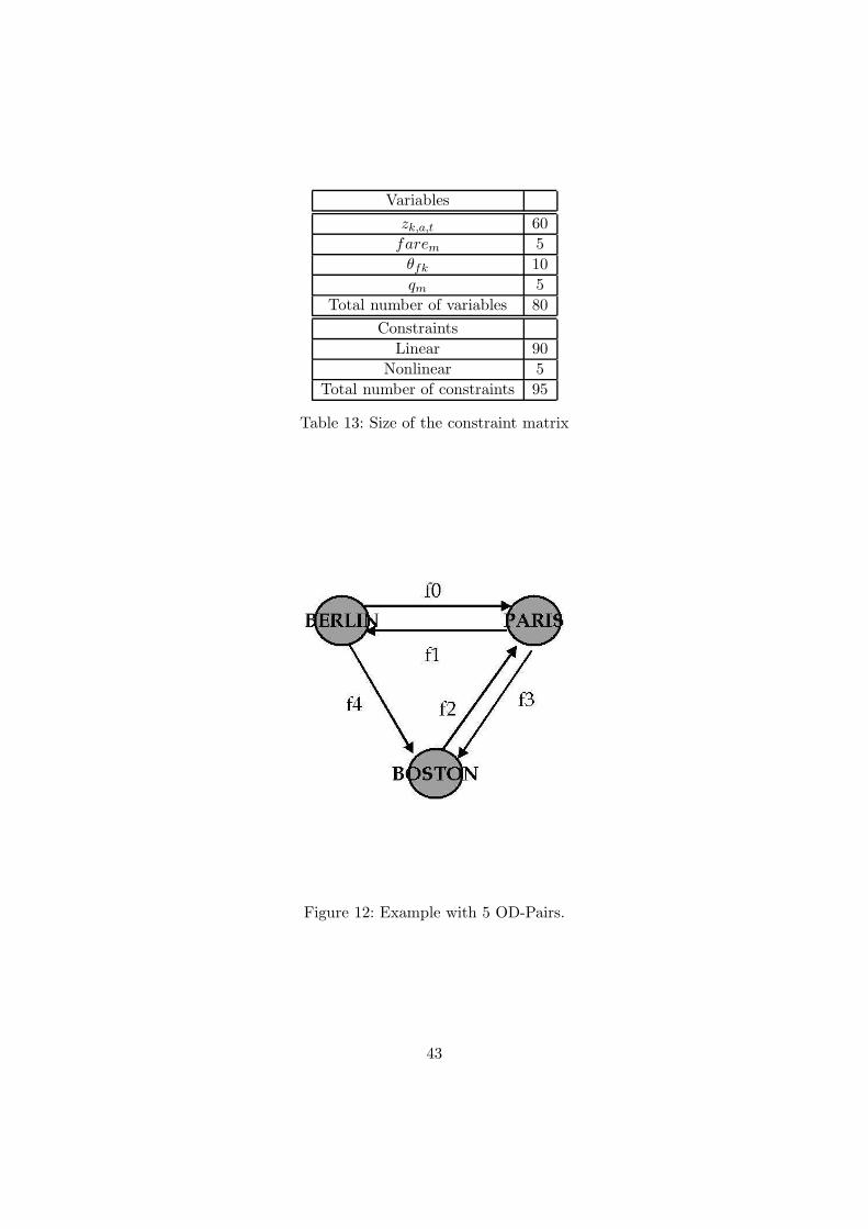
Variables

zk,a,t 60

farem 5

θfk 10

qm 5

Total number of variables 80

Constraints

Linear 90

Nonlinear 5

Total number of constraints 95

Table 13: Size of the constraint matrix

Figure 12: Example with 5 OD-Pairs.

43

Figure 13: Time line Network for the example with 5 OD-pairs.

44

UTILITY Value

U0 20

U1 23

U2 21

U3 24

U4 29

U5 49

DEMAND FACTOR

ω0 20

ω1 23

ω2 18

ω3 20

ω4 35

ASSIGNMENT COST

costa00 10

costa01 20

costa10 12

costa11 19

costa20 38

costa21 43

costa30 46

costa31 23

costa40 48

costa41 50

PASSENGER COST

costm0 10

costm1 15

costm2 17

costm3 16

costm4 23


cap0 50

cap1 40

Table 14: Parameters for an example with 5 OD Pairs

45

OUTCOME PERCENTAGE OF CALLS

Current point can not be improved upon. 5%First-Order-Kuhn-Tucker constraints are not satisfied

Convergence to the optimum convergence point 80%

Large error in the derivatives 5%

Convergence to other convergence points 10%

Table 15: Approximative evaluation of the performance to find the starting point of theBranch-And-Bound.

θfk farem qm objfun

θ00 = 0 fare0 = 38 q0 = 0 621.535666

θ01 = 0 fare1 = 20 q1 = 0

θ10 = 0 fare2 = 39 q2 = 0

θ11 = 0 fare3 = 39 q3 = 0

θ20 = 0 fare4 = 42.707412 q4 = 0.692170

θ21 = 0

θ30 = 0

θ31 = 0

θ40 = 0.692170

θ41 = 0

Table 16: Starting point for the Branch-And-Bound algorithm.

does not converge, either the starting point implies a large error in the nonlinear con-straints or the final point can not be improved upon and does not satisfy the first orderof Kuhn-Tucker condition. But if it converges, the final point is always the same, shownin table 16.

Afterwards we try base schedules that include couples of flight legs, as input of theSQP function. When the SQP function does not converge, we modify each price offlight legs or assignment variables to improve the final schedule. When it converge,we have found 2 distinct optimum, one with an objective function value of 533.989454and another with 621.535666. The table 15 shows an approximative evaluation of theperformance of the first call of the SQP function. The SQP function converges in 90%of the cases.

The best objective function value was 621.535666. We choose this final solution to bethe root of the Branch-and-Bound algorithm.

7.4 Performance of the Branch-And-Bound algorithm

Given the previous starting point, we analyse the performance of the Branch-and-Boundalgorithm. In this example, the search tree of the Branch-and-Bound algorithm has 215

leaves in the worst case, if no fathoming is operated. We consider that the number of

46


θ00 = 0 fare0 = 38 q0 = 0 618.989454

θ01 = 0 fare1 = 20 q1 = 0

θ10 = 0 fare2 = 37.973351 q2 = 0

θ11 = 0 fare3 = 37.221707 q3 = 0

θ20 = 0 fare4 = 43.056842 q4 = 1

θ21 = 0

θ30 = 0

θ31 = 0

θ40 = 1

θ41 = 0

Table 17: Output of the Branch-And-Bound algorithm.

covered nodes represents the number of iterations of the algorithm.

The number of available aircrafts can limit the number of covered nodes. For example,we suppose q1 = 0, 5, q2 = 0, 5 and q3 = 0, 5. Since there are only 2 aircrafts only 2q-values can be set to 1. Or else the schedule will not be feasible (flight leg included inthe schedule but not assigned or a flight leg non-included but assigned). That allows todrop the leaf q1 = 1, q2 = 1, q3 = 1 in the tree. In our heuristic, the SQP function willfind the subproblem unfeasible. If we reduce the size of the search tree before operation,we can save unnecessary calls of the SQP function. This pre-processing makes the al-gorithm more complex in terms of memory storage and branching strategy. Constraintsfor feasible nodes have to be stored before operation and the current node has to fulfillthose stored requirements at each iteration.

The SQP function has now converged in less than 20% of the calls, because most ofthem are no good starting points for the SQP function. As far as the performance ofthe Branch-And-Bound algorithm is concerned, the depth first strategy allows to finda feasible solution after two iterations. When we mention iterations, we do not meanbranching. After another iteration, the best first strategy leads to the optimum, dis-played in table 18. With the current upper bound the branch with θ40 = 0 is fathomed.After 4 iterations, the Branch-And-Bound algorithm stops. As expected, the best so-lution is the one with the variables θ40 and q4 set to 1. Compared to the root of theBranch-and-Bound, the objective function has decreased but the price of the flight 4 hasbeen increased. But if we compare with the schedule before the first call of the SQPfunction, the objective function has increased of 9% (565.934055 to 618.989454).

Two flights (f2 and f4) are now mandatory flights. The first call of the SQP convergesin 75% of times to distinct points. We will start the Branch-And-Bound algorithm witha feasible ”bad” solution shown in table 18 regarding to the objective function value.The SQP function converges in less than 8% of the cases. The Branch-and-Bound algo-

47


θ00 = 1 fare0 = 27.000004 q0 = 0 307.650319

θ01 = 0 fare1 = 21.038100 q1 = 0

θ10 = 0.7897521 fare2 = 42.793679 q2 = 0.887961

θ11 = 0 fare3 = 27.000000 q3 = 0

θ20 = 1 fare4 = 60.210052 q4 = 0.996996

θ21 = 0

θ30 = 0

θ31 = 0.897212

θ40 = 0

θ41 = 1

Table 18: ”Bad” starting point for the Branch-And-Bound algorithm.


θ00 = 1 fare0 = 27.000004 q0 = 0 293.286222

θ01 = 0 fare1 = 21.038100 q1 = 0

θ10 = 1 fare2 = 42.793679 q2 = 1

θ11 = 0 fare3 = 27.000000 q3 = 0

θ20 = 1 fare4 = 60.210052 q4 = 1

θ21 = 0

θ30 = 0

θ31 = 0

θ40 = 0

θ41 = 1

Table 19: Output of the Branch-And-Bound algorithm with a ”bad” starting point.

rithm founds an optimum, displayed in table 18, after 13 iterations. If we set q1 = 0.5,the algorithm iterates 18 times and the SQP function converges in less than 12% of thecases. The final point is the same as the former one.

If we set q1 = 0.5 and q0 = 0.5, the fare4 has been lightly improved to 60.210051after 26 iterations.If we stop the algorithm before 38 iterations, the final point is not optimum and can befar from the optimum. But if we choose a starting point with values close to 0 or 1, theBranch-And-Bound will converge faster to the optimum. In this example, we can reducethe number of iterations of the Branch-and-Bound algorithm to 36.

7.5 Truncated Branch-And-Bound algorithm

For larger problems, we will not be able to run the Branch-and-Bound until it findsthe optimum, because the number of nodes grows exponentially. We apply a truncated

48

UNKNOWN VARIABLES NB MAX ITERATIONS CONVERGENCE OF SQP

2 4 20% − 30%

5 19 less than 12%

6 26 less than 8%

9 40 less than 6%

Table 20: Performance of the complete algorithm with five OD-Pairs.

Branch-and-Bound instead. We stop the algorithm when a feasible ”good” solution isfound. That is why our implementation is a heuristic. The difficulty is to find the cri-teria that determines when a solution close to the optimum is met. A limited numberof iterations that depends on the size of the problem is a wrong approach. We can notsuppose that after the Branch-and-Bound algorithm covers 60% of the search tree, thena ”good” suboptimum has been met. This upper bound does not fit to the nonlinearaspect of our model.

An alternative could be to set a time limit for the Branch-And-Bound algorithm. Itrelies on the running time of the SQP function. With the percentage of convergence, thesize of the tree and the running time of each outcome, we can estimate the maximumrunning time of the Branch-and-Bound. In our example, the SQP function converges lessthan 8% and does not fulfill Kuhn-Tucker constraint around 70% of times (that takesone second). The rest of the time, the function loops through a maximum number of516 iterations and than stops (that takes 3 seconds). Given this data, we can determinea time limit for the algorithm, before a suboptimum is found.

Another alternative is to operate in two phases. First the problem is solved with agreedy algorithm, in order to obtain an objective function value of a good feasible solu-tion that we store for the second phase. Then we run our Branch-and-Bound algorithm,where we compare the objective function of the current feasible solution to the storedvalue. We consider that we have found a good solution, when both values are ”closeenough”. We fix a maximal difference between the upper bound and the expected fea-sible solution prior to the operation of the Branch-and-Bound. This maximal differencedefines the stopping criteria.

This last approach is the most suitable but costs more than the other alternatives interms of processing time because two algorithms are operated. To reduce this costs, wecan start the Branch-and-Bound before the greedy algorithm. Or as upper bound for thetruncated Branch-and-Bound, we can consider the root of the Branch-and-Bound algo-rithm, because the Branch-and-Bound algorithm will not improve the objective functionof the root. The root is an optimum of the optimization problem, where θfk and qm arerelaxed. In practice, a good feasible solution is found, when the difference in objectivefunction values is less than 20% of the objective function value of the root.

In this last section, we have made the following observations to the performance of

49

the complete algorithm:

(1) The performance of the Branch-And-Bound, in terms of numbers of iterations untilthe optimum is found, based on the choice of the starting point.

(2) We can save calls of the SQP function by eliminating unfeasible leaves beforeoperation. But this requires memory storage.

(3) A good criteria to find a feasible solution close to the optimum, is difficult becauseof the exponential growth of the problem size. A good solution is to solve theproblem in two stages: the first time to find an upper bound, that will be comparedto the current solution of the Branch-and-Bound in a second time.

8 Conclusion

8.1 Summary of contributions

The objective of this diploma thesis was to build a model integrating Airline ScheduleDesign and Product Line Design. Our model solves an incremental integrated airlineschedule generation and fleet assignment problem along with the pricing problem con-sidering customer preference. A base schedule, composed by mandatory and optionalflight legs, is given as input. Our model maximizes the profit of the airline, while addingand deleting optional flight legs. The airline schedule design model integrates model ofLohatepannont M. and Barnhart C. [4] for the airline schedule design with choice-basedproduct line design at product and attribute level.The formulated problem is a Mixed Integer Nonlinear problem with large number of de-cision variables and sets of constraints. Due to the size and complexity of the problem,we aim to implement a heuristic to find a solution close to the optimum. Our solutionapproach was to decompose the model into nonlinear part and integer part. We imple-ment a Branch-And-Bound algorithm, for the integer part, that solves at each branchthe nonlinear part with integer variables fixed, with a sequential quadratic program-ming function. We use the library of the Numerical Algorithms Group to implement thesequential quadratic programming method. We implement by ourselves a Branch-And-Bound with a depth first combined with a best first tree search strategy.In the example with two flight legs, we have shown that the convergence of the SQPfunction is sensitive to the choice of the initial point. We have also shown the influenceof the consumer preference on the optimal solution. Our model captures always theflow of passenger that optimizes the profit. In the example with 5 OD-pairs, the moreinteger variables are to determine, the less is the percentage of convergence for the SQPfunction. For larger problems, we have tried to find a stopping criteria for a truncatedBranch-and-Bound. The stopping criteria depends on the difference between the objec-tive function value of the root (of the Branch-and-Bound) and the one of the currentfeasible solution. A difference in objective function values of less than 20% of the profitcorresponding to the root implies that a feasible good solution is met.

50

8.2 Future Research Directions

This thesis represents a contribution in the area of market-oriented airline schedule de-sign. There are many research questions left unexplored.In the short term, case studies to measure the sensitivity of MNL and BTL model atitinerary and itinerary attributes level must be performed. The results will allow usto validate our approach with the conjoint analysis. Otherwise, we should express theconsumer preference by an other alternative than conjoint analysis, such as a linear orsemi-linear utility.In the medium term, supposing that our model has been validated, we should enableour incremental model to perform re-schedule with time-windows in addition to addi-tions/deletions. This will fine-tune the optimization of the base schedule.In the long term, we can concentrate on improving our implementation with the followingresearch directions:

- Apply the an integrated algorithm realized by Leyffer [20] to our model.This requires the self-implementation of the SQP function. This will enable theBranch-And-Bound to branch before an iteration of the SQP solver. This cansignificantly speed up our implementation.

- Implement a solution with genetic algorithm. This requires to find anadapted mutation and recombination functions for the itineraries.

51

Notations

PARAMETERS

General:A: Set of airports, indexed by a.K: Set of aircrafts, indexed by k.Nk: Number of aircrafts in fleet-type k.Nm: Number of flight legs in itinerary m.N : Set of attributes of an itinerary, with the price as first attribute and the other at-tributes are service-oriented.N1: Set of attributes of an itinerary, indexed by n.Jn: Set of level sets for the attribute n, indexed by j. J0 is the set of possible prices.P : Set of nodes of the underlying network. A node is composed by a time, an airportand an aircraft, indexed by k, a, tT : Sorted set of all event.Itineraries:M : Set of itineraries including null itinerary, indexed by m.MO: Set of itineraries containing optional flight, indexed by mit m.MC : Set of competitive itineraries.

Flight legs:

Ωm: Set of flight legs in itinerary m, indexed by f .Ω: Set of flight legs in the flight schedule, indexed by f .ΩM : Set of mandatory flight legs in the flight schedule, indexed by f .ΩO: Set of optional flight legs in the flight schedule, indexed by f .Ωk: Set of flight legs that pass the count time when flown by fleet-type k.I(k, a, t): Set of inbound flight legs to node k, a, t.O(k, a, t): Set of outbound flight legs to node k, a, t.cfk: Cost for the assignment of the aircraft k to the flight leg f .cm: Cost pro passenger.capk: Number of seats in the aircraft k.demm: Demand for the itinerary m. These represents all the passengers that want totravel from origin-airport to destination-airport regardless of the operational constraints.That is called the unconstraint demand.δfm: = 1, when the itinerary m includes the flight leg f , = 0 otherwise.

Preference measurement:

Udm: Service related utility of the passenger d for the itinerary m. This utility is inde-pendent of the price.Ud0: Given utility of passenger segment d for competitive itineraries.pdm: Product demands or market shares described by the probability that the passenger

52

d choose the itinerary m.ωd: Size of the segment d.

DECISION VARIABLES

Schedule generation and fleet assignment:

qm: = 1, if itinerary m is included in the flight schedule, =0, otherwise.θfk: = 1, when the flight leg f is flown with the aircraft k, = 0 otherwise.zk,a,t+ : The number of aircraft k on the ground at the airport a immediately after timet.zk,a,t− : The number of aircraft k on the ground at the airport a immediately before timet.If t1 and t2 are the times associated with adjacent events then zk,a,t+

1

= zk,a,t−2

.

Pricing model:

farem: Price charged to every passenger on the itinerary m. We make a slight abuse ofnotation by modelling the price of a flight leg with the same variable but indexed withf .xjnm: = 1, when the n-th attribute is assigned to the j-th level in the itinerary m, = 0otherwise. These are binary constants for m ∈ M c (competitive itineraries) and binarydecision variables for m ∈ M .xj0m: =1, when a passenger is charged with the j-th possible price for itinerary m.farejm: j-th level of the price for the itinerary m.

53

Annexe

- Derivatives with respect to farem for a given m

f = e(Um−farem)qmωm

1M∑

m1=1

e(Um1−farem1

)qm1+ U0

+ (farem − cm)

e(Um−farem)qm −

M∑

m1=1

e(Udm1−farem1

)qm1− U0

(

M∑

m1=1

e(Um1−farem1

)qm1+ U0)

2

+

M∑

m2 6=m

qme(Um−farem) (farem2− cm2

)e(Um2−farem2

)qm2ωm

(

M∑

m1=1

e(Um1−farem1

)qm1+ U0)

2

c1 =

δfme(Um−farem)

e(Udm−farem)qm −

M∑

m1=1

e(Um1−farem1

)qm1− U0

(

M∑

m1=1

e(Um1−farem1

)qm1+ U0)

2

+

M∑

m2 6=m

e(Um−farem) e(Um2−farem2

)qm2δfm2

ωm

(

M∑

m1=1

e(Um1−farem1

)qm1+ U0)

2

- Derivatives with respect to zk,a,t for a given k, a, t

f = 0

c1 =

K∑

k=1

capk

- Derivatives with respect to θfk for given f and k

f = −cfk

c1 = 0

54

- Derivatives with respect to qm for given m

f =

(farem − cmωme(Um−farem)

M∑

m1=1

e(Um1−farem1

)qm1+ U0 − qme(Um−farem)

(

M∑

m1=1

e(Um1−farem1

)qm1+ U0)

2

−M∑

m2 6=m

e(Um−farem) (farem2− cm2

)e(Um2−farem2

)qm2ωm2

(M∑

m1=1

e(Um1−farem1

)qm1+ U0)

2

c1 =

δfmωme(Um−farem)

M∑

m1=1

e(Um1−farem1

)qm1+ Ud0 − qme(Udm−farem)

(

M∑

m1=1

e(Um1−farem1

)qm1+ U0)

2

−M∑

m2 6=m

e(Um−farem) e(Um2−farem2

)δfm2qm2

ωm

(M∑

m1=1

e(Um1−farem1

)qm1+ U0)

2

55

References

AIRLINE SCHEDULE DESIGN

Overview of airline schedule planning problem:

[1] Barnhart C., Cohn A. (2004), Airline Schedule Planning: Accomplishments and

Oppertunities, MANUFACTURING SERVICE OPERATIONS MANAGEMENT,Vol. 6, No. 1, Winter 2004, 3-22.

Airline schedule models with passenger behaviour model:

[2] Dobson G., Lederer P. (1993), Airline Scheduling and Routing in a Hub-and-

Spoke System, Transportation Science, Vol. 27, 281-297.

[3] Teodorovic D., Kremar-Nozic E.(1989), Multicriteria models to determine

flight frequencies on an airline network under competitive conditions, Transporta-tion Science 23 (1), 14-25

Integrated airline schedule models:

[4] Lohatepanont M., Barnhart C. (2004), Airline Schedule Planning: Integrated

Models and Algorithms for Schedule Design and Fleet Assignment, TransportationScience, Vol. 38, 19-32.

[5] Brueckner J., Zhang Y. (2001), A Model of Scheduling in Airline Networks,Journal of Transport Economics and Policy, Vol. 35, Part 2, May 2001, 195-222

[6] Erdmann A., Nolte A., Noltemeier A., Schrader R. (1999), Modelling and

Solving the Airline Schedule Generation Problem, Working Paper, ZAIK Universityof Cologne.

[7] Soumis P., Ferland J.A., Rousseau M. (1980), A Model for Large Scale Aircraft

Routing and Scheduling Problems, Transportation Research, No. 14B, 191-201.

[8] Barnhart C., Lu F., Shenoi R. (1998), Integrated airline schedule planning,Operations Research in the Airline Industry, 9, 384-403.

[9] Klabdjan D. (2003), Large-scale models in the airline indus-

try, Column Generation, Kluwer Academic Publishers. Available athttps://netfiles.uiuc.edu/klabjan/www.

Implementation of airline schedule planning problem:

[10] Grosche T., Heinzl A. (2003), Simultane Erstellung von Fluganen mit Genetis-

chen Algorithmen, Working Papers in Information Systems, Working Paper 8 /March 2003, University of Mannheim

[11] Mathaisel D. (1997), Decision Support for Airline Schedule Planning, Journal ofCombinational Optimization 1, 251-275

56

PRODUCT LINE DESIGN

[12] Dobson G., Kalish S. (1998), Positionning and Pricing a Product Line, Market-ing Science 2 (2), 107-124

[13] Gaul W., Aust E., Baier D. (1995), Gewinnorientierte Produktliniengestaltung

unter Berucksichtigung des Kundennutzens, Zeitschrift fur Betriebswirtschaft 65(8), 835-855.

[14] Green P.E., Krieger A.M.(1985), Models and Heuristics for Product Line Se-

lection, Marketing Science 4 (1), 1-19

[15] Kohli R., Krishnamurti R.(1989), Optimal product design using conjoint analy-

sis: Computational complexity and algorithms, European Journal of OperationalResearch 40, 186-195

[16] Natter M., Feurstein M.(2001), Real World Performance of Choice-Based Con-

joint Models, Report Series, Report No. 58, June 2001, Vienna University of Eco-nomics and Business Administration

[17] Oppewal H., Louviere J. J., Timmermans H.(1994), Modeling Hierarchical

Conjoint Processes with Integrated Choice Experiments, Journal of Marketing Re-search, Vol. 31, 1994, 92-105

[18] Green P.E., Krieger A. M., Agarwal M. K.(1991), Adaptive Conjoint Analy-

sis: Some Caveats and Suggestions, Journal of Marketing Research, Vol. 28, 1991,215-222

[19] Kohli R., Sukumar R.(1990), Heuristics for Product Line Design Using Conjoint

Analysis, Managemenent Science, Vol. 36(12), December, 1464-1478

[20] Leyffer S.(1998), Integrating QP and branch-and-bound for Mixed Integer Non-

linear Programming, 1998, 1-13

[21] Eliashberg J., Lilien G.L.(1998), Marketing, Handbooks in Operations Researchand Management Science, Volume 15, 467-515

57

Documents

Airline Schedule Planning - KITcrypto.iti.kit.edu/fileadmin/User/calmet/stdip/dip-rabentanety.pdf · Product Line Design Universit¨at Karlsruhe ... 4.2.1 Passenger Mix Model