Embed Size (px)
Citation preview
KINETICS OF GRAPHITE OXIDATION IN REACTINGFLOW FROM IMAGING FOURIER TRANSFORM
SPECTROSCOPY
DISSERTATION
Ashley E. Gonzales, Captain, USAF
AFIT-ENP-DS-16-S-024
DEPARTMENT OF THE AIR FORCEAIR UNIVERSITY
AIR FORCE INSTITUTE OF TECHNOLOGY
Wright-Patterson Air Force Base, Ohio
DISTRIBUTION STATEMENT A
APPROVED FOR PUBLIC RELEASE; DISTRIBUTION UNLIMITED.

The views expressed in this document are those of the author and do not reflect theofficial policy or position of the United States Air Force, the United States Departmentof Defense or the United States Government. This material is declared a work of theU.S. Government and is not subject to copyright protection in the United States.
AFIT-ENP-DS-16-S-024
KINETICS OF GRAPHITE OXIDATION IN REACTING FLOW FROM IMAGING FOURIER
TRANSFORM SPECTROSCOPY
DISSERTATION
Presented to the Faculty
Graduate School of Engineering and Management
Air Force Institute of Technology
Air University
Air Education and Training Command
in Partial Fulfillment of the Requirements for the
Degree of Doctor of Philosophy in Optical Sciences and Engineering
Ashley E. Gonzales, MS
Captain, USAF
XXXX 2016
DISTRIBUTION STATEMENT A
APPROVED FOR PUBLIC RELEASE; DISTRIBUTION UNLIMITED.
AFIT-ENP-DS-16-S-024
KINETICS OF GRAPHITE OXIDATION IN REACTING FLOW FROM IMAGING FOURIER
TRANSFORM SPECTROSCOPY
DISSERTATION
Ashley E. Gonzales, MSCaptain, USAF
Committee Membership:
Glen P. Perram, PhDChair
Kevin C. Gross, PhDMember
Marc D. Polanka, PhDMember
AFIT-ENP-DS-16-S-024
Abstract
This work focuses on the characterization of laser irradiated graphite oxidation
using mid-wave infrared (MWIR) imaging Fourier transform spectroscopy (IFTS). Al-
though graphite oxidation has been studied extensively, IFTS uniquely provides spatial
characterization of the reacting plumes. Spatial maps of species and temperature pro-
vide much needed insight into the transport and kinetic mechanisms and are vital for
validation of numerical efforts. The current study builds on previous work using IFTS
to characterize graphite oxidation in buoyant flow. Buoyant flow measurements are
expanded to a wider range of graphite materials and surface temperatures. Oxidation
in flat plate shear flow and stagnation flow are also evaluated to determine the role of
transport.
Samples were heated using a 1.07 µm continuous wave (CW) fiber laser. The ox-
idation plume was observed using MW IFTS camera at spectral resolution of 2 cm-1
and spatial resolution of 0.5 mm/pixel with framing rates of 1 Hz. Spectral signatures
featured emission from C O and C O2 in the 1800 - 2500 cm-1 spectral region. A two
layer radiative transfer model (RTM) using the CDSD-4000 and HITEMP cross-section
databases was used to infer spatial maps of temperature and species (C O , C O2 ) con-
centration from spectral data.
Buoyant flow work is an extension of previous work by Acosta [1]. Graphite samples
of varying porosity are irradiated at 1000 and 3600 W/cm2 producing surface temper-
atures of 1000 - 4000 K and 3-8 mm thick reacting plumes. Plume temperatures are
found to be in non-equilibrium with surface temperatures, peaking at 2500 K. C O
population was found to be highly correlated with surface temperature as a result of the
Cs +O2⇒ 2C O and Cs +C O2⇒ 2C O surface reactions. A decline in C O2 population
4
was observed near laser center due to the Cs +C O2⇒ 2C O reaction. The [C O ]/[C O2]
product ratios show a general trend of: [C O ]/[C O2] = 22 exp(−6000/Ts ).
Graphite oxidation in a flat plate shear flow was observed at flow speeds of 5 - 10
m/s (R e < 7 ·104). Samples were irradiated at 750 and 1500 W/cm2, resulting in surface
temperatures of 1000 - 4000 K and 2- 4 mm thick reacting plumes. Plume temperatures
are again found to be in non-equilibrium with surface temperatures, peaking at 2500
K. C O population was again shown to be highly correlated with surface temperature,
with some asymmetry due to flow effects. The decline in C O2 population due to the
Cs +C O2 ⇒ 2C O reaction is less pronounced than in the buoyant case, but can still
be observed at laser center. The [C O ]/[C O2] product ratios show a general trend of:
[C O ]/[C O2] = 8exp(−3100/Ts ). This data set represents the first spatially resolved
measurements of graphite oxidation in a flat plate shear flow.
Graphite oxidation in a stagnation flow (v = 1.5 m/s) was observed at surface tem-
peratures of 1500 - 3100 K, resulting in reacting layers on the order of 1 - 3 mm thick.
The [C O ]/[C O2] product ratios show two general trends. At lower temperatures, re-
sults compare favorably with previous results with a general trend of [C O ]/[C O2] =
2exp(−2400/Ts ). At higher temperatures (2200- 2500 K), the [C O ]/[C O2] ratios tran-
sition to higher effective activation energies of 16,000 and 31,000 K. This transition
coincides with the decline in C O2 and rise in C O , suggesting it is a result of the Cs −C O2
reaction. This transition takes place at different temperatures for each of the three cases,
possibly due to varying C O population which has been shown to inhibit the Cs −C O2
reaction. This data set represents the first spatially resolved measurements of graphite
oxidation in a stagnation flow.
5
Table of Contents
Page
Abstract . . . . . . . . . . . . . . . . . . . . . . . . . . . . . . . . . . . . . . . . . . . . . . . . . . . . . . . . . . . . . . . . . . . . . . . . . . . . . . . . . 4
List of Figures . . . . . . . . . . . . . . . . . . . . . . . . . . . . . . . . . . . . . . . . . . . . . . . . . . . . . . . . . . . . . . . . . . . . . . . . . . . 9
List of Tables . . . . . . . . . . . . . . . . . . . . . . . . . . . . . . . . . . . . . . . . . . . . . . . . . . . . . . . . . . . . . . . . . . . . . . . . . . 15
I. Introduction . . . . . . . . . . . . . . . . . . . . . . . . . . . . . . . . . . . . . . . . . . . . . . . . . . . . . . . . . . . . . . . . . . . . . . . 1
1.1 Research Objectives . . . . . . . . . . . . . . . . . . . . . . . . . . . . . . . . . . . . . . . . . . . . . . . . . . . . . . . . . . 21.2 Document Outline . . . . . . . . . . . . . . . . . . . . . . . . . . . . . . . . . . . . . . . . . . . . . . . . . . . . . . . . . . . 4
II. Background. . . . . . . . . . . . . . . . . . . . . . . . . . . . . . . . . . . . . . . . . . . . . . . . . . . . . . . . . . . . . . . . . . . . . . . . 6
2.1 Summary . . . . . . . . . . . . . . . . . . . . . . . . . . . . . . . . . . . . . . . . . . . . . . . . . . . . . . . . . . . . . . . . . . . . . 62.2 Carbon Oxidation . . . . . . . . . . . . . . . . . . . . . . . . . . . . . . . . . . . . . . . . . . . . . . . . . . . . . . . . . . . . 6
Overview . . . . . . . . . . . . . . . . . . . . . . . . . . . . . . . . . . . . . . . . . . . . . . . . . . . . . . . . . . . . . . . . . . . . . . 6Graphite . . . . . . . . . . . . . . . . . . . . . . . . . . . . . . . . . . . . . . . . . . . . . . . . . . . . . . . . . . . . . . . . . . . . . . 7CO Oxidation . . . . . . . . . . . . . . . . . . . . . . . . . . . . . . . . . . . . . . . . . . . . . . . . . . . . . . . . . . . . . . . . . 8C(s ) Oxidation . . . . . . . . . . . . . . . . . . . . . . . . . . . . . . . . . . . . . . . . . . . . . . . . . . . . . . . . . . . . . . . . . 9[C O ]/[C O2] Temperature Dependence . . . . . . . . . . . . . . . . . . . . . . . . . . . . . . . . . . . . 14
2.3 Fourier Transform Spectroscopy . . . . . . . . . . . . . . . . . . . . . . . . . . . . . . . . . . . . . . . . . . . 15Radiative Transfer Model . . . . . . . . . . . . . . . . . . . . . . . . . . . . . . . . . . . . . . . . . . . . . . . . . . . 18
2.4 Flow Conditions . . . . . . . . . . . . . . . . . . . . . . . . . . . . . . . . . . . . . . . . . . . . . . . . . . . . . . . . . . . . 19Flat Plate Shear Flow . . . . . . . . . . . . . . . . . . . . . . . . . . . . . . . . . . . . . . . . . . . . . . . . . . . . . . . 19Buoyant Flow . . . . . . . . . . . . . . . . . . . . . . . . . . . . . . . . . . . . . . . . . . . . . . . . . . . . . . . . . . . . . . . 22Stagnation Flow . . . . . . . . . . . . . . . . . . . . . . . . . . . . . . . . . . . . . . . . . . . . . . . . . . . . . . . . . . . . 25
III. Oxidation Model . . . . . . . . . . . . . . . . . . . . . . . . . . . . . . . . . . . . . . . . . . . . . . . . . . . . . . . . . . . . . . . . 28
3.1 Conservation Equations . . . . . . . . . . . . . . . . . . . . . . . . . . . . . . . . . . . . . . . . . . . . . . . . . . . . 283.2 1D Model . . . . . . . . . . . . . . . . . . . . . . . . . . . . . . . . . . . . . . . . . . . . . . . . . . . . . . . . . . . . . . . . . . . 29
Surface Temperature Sensitivity . . . . . . . . . . . . . . . . . . . . . . . . . . . . . . . . . . . . . . . . . . . 32Flame Length Sensitivity . . . . . . . . . . . . . . . . . . . . . . . . . . . . . . . . . . . . . . . . . . . . . . . . . . . 33Surface Rate Sensitivity . . . . . . . . . . . . . . . . . . . . . . . . . . . . . . . . . . . . . . . . . . . . . . . . . . . . . 33
3.3 Quasi 2D Model . . . . . . . . . . . . . . . . . . . . . . . . . . . . . . . . . . . . . . . . . . . . . . . . . . . . . . . . . . . . 34Surface Temperature Sensitivity . . . . . . . . . . . . . . . . . . . . . . . . . . . . . . . . . . . . . . . . . . . 36Flow Sensitivity . . . . . . . . . . . . . . . . . . . . . . . . . . . . . . . . . . . . . . . . . . . . . . . . . . . . . . . . . . . . . 36
IV. Experimental Methods . . . . . . . . . . . . . . . . . . . . . . . . . . . . . . . . . . . . . . . . . . . . . . . . . . . . . . . . . . 42
4.1 Laser System and Diagnostics . . . . . . . . . . . . . . . . . . . . . . . . . . . . . . . . . . . . . . . . . . . . . . 424.2 Graphite Materials . . . . . . . . . . . . . . . . . . . . . . . . . . . . . . . . . . . . . . . . . . . . . . . . . . . . . . . . . . 434.3 Diagnostics . . . . . . . . . . . . . . . . . . . . . . . . . . . . . . . . . . . . . . . . . . . . . . . . . . . . . . . . . . . . . . . . . 43
6
Page
Thermal Imagery . . . . . . . . . . . . . . . . . . . . . . . . . . . . . . . . . . . . . . . . . . . . . . . . . . . . . . . . . . . 43Imaging Fourier Imaging Spectrometer . . . . . . . . . . . . . . . . . . . . . . . . . . . . . . . . . . . . 49Visible Imagery . . . . . . . . . . . . . . . . . . . . . . . . . . . . . . . . . . . . . . . . . . . . . . . . . . . . . . . . . . . . . 55
4.4 Flow Variations . . . . . . . . . . . . . . . . . . . . . . . . . . . . . . . . . . . . . . . . . . . . . . . . . . . . . . . . . . . . . 55Buoyant Flow . . . . . . . . . . . . . . . . . . . . . . . . . . . . . . . . . . . . . . . . . . . . . . . . . . . . . . . . . . . . . . . 55Flat Plate Shear Flow . . . . . . . . . . . . . . . . . . . . . . . . . . . . . . . . . . . . . . . . . . . . . . . . . . . . . . . 56Stagnation Flow . . . . . . . . . . . . . . . . . . . . . . . . . . . . . . . . . . . . . . . . . . . . . . . . . . . . . . . . . . . . 56
V. Imaging Fourier Transform Spectroscopy of Graphite Oxidationin a Buoyant Flow . . . . . . . . . . . . . . . . . . . . . . . . . . . . . . . . . . . . . . . . . . . . . . . . . . . . . . . . . . . . . . . 60
5.1 Abstract . . . . . . . . . . . . . . . . . . . . . . . . . . . . . . . . . . . . . . . . . . . . . . . . . . . . . . . . . . . . . . . . . . . . . 605.2 Introduction . . . . . . . . . . . . . . . . . . . . . . . . . . . . . . . . . . . . . . . . . . . . . . . . . . . . . . . . . . . . . . . . 615.3 Experimental . . . . . . . . . . . . . . . . . . . . . . . . . . . . . . . . . . . . . . . . . . . . . . . . . . . . . . . . . . . . . . . 64
Materials . . . . . . . . . . . . . . . . . . . . . . . . . . . . . . . . . . . . . . . . . . . . . . . . . . . . . . . . . . . . . . . . . . . 65Plume Measurements . . . . . . . . . . . . . . . . . . . . . . . . . . . . . . . . . . . . . . . . . . . . . . . . . . . . . . 66Thermal Measurements . . . . . . . . . . . . . . . . . . . . . . . . . . . . . . . . . . . . . . . . . . . . . . . . . . . . 68
5.4 Experimental Results and Discussion . . . . . . . . . . . . . . . . . . . . . . . . . . . . . . . . . . . . . . 69Emissivity . . . . . . . . . . . . . . . . . . . . . . . . . . . . . . . . . . . . . . . . . . . . . . . . . . . . . . . . . . . . . . . . . . . 69Surface Temperature . . . . . . . . . . . . . . . . . . . . . . . . . . . . . . . . . . . . . . . . . . . . . . . . . . . . . . . 70Plume Properties . . . . . . . . . . . . . . . . . . . . . . . . . . . . . . . . . . . . . . . . . . . . . . . . . . . . . . . . . . . 72Diffusion . . . . . . . . . . . . . . . . . . . . . . . . . . . . . . . . . . . . . . . . . . . . . . . . . . . . . . . . . . . . . . . . . . . . 77Temperature Dependence of [C O ]/[C O2] Ratio . . . . . . . . . . . . . . . . . . . . . . . . . . . 79
5.5 Model . . . . . . . . . . . . . . . . . . . . . . . . . . . . . . . . . . . . . . . . . . . . . . . . . . . . . . . . . . . . . . . . . . . . . . . 805.6 Model Results and Discussion . . . . . . . . . . . . . . . . . . . . . . . . . . . . . . . . . . . . . . . . . . . . . 83
[C O ]/[C O2] Temperature Dependence . . . . . . . . . . . . . . . . . . . . . . . . . . . . . . . . . . . . 84Non-uniqueness . . . . . . . . . . . . . . . . . . . . . . . . . . . . . . . . . . . . . . . . . . . . . . . . . . . . . . . . . . . . 85
5.7 Conclusions . . . . . . . . . . . . . . . . . . . . . . . . . . . . . . . . . . . . . . . . . . . . . . . . . . . . . . . . . . . . . . . . 86
VI. Imaging Fourier Transform Spectroscopy of Graphite Oxidationin a Flat Plate Shear Flow . . . . . . . . . . . . . . . . . . . . . . . . . . . . . . . . . . . . . . . . . . . . . . . . . . . . . . . . 89
6.1 Abstract . . . . . . . . . . . . . . . . . . . . . . . . . . . . . . . . . . . . . . . . . . . . . . . . . . . . . . . . . . . . . . . . . . . . . 896.2 Introduction . . . . . . . . . . . . . . . . . . . . . . . . . . . . . . . . . . . . . . . . . . . . . . . . . . . . . . . . . . . . . . . . 906.3 Experimental . . . . . . . . . . . . . . . . . . . . . . . . . . . . . . . . . . . . . . . . . . . . . . . . . . . . . . . . . . . . . . . 91
Overview . . . . . . . . . . . . . . . . . . . . . . . . . . . . . . . . . . . . . . . . . . . . . . . . . . . . . . . . . . . . . . . . . . . . 91Materials . . . . . . . . . . . . . . . . . . . . . . . . . . . . . . . . . . . . . . . . . . . . . . . . . . . . . . . . . . . . . . . . . . . 93Plume Measurements . . . . . . . . . . . . . . . . . . . . . . . . . . . . . . . . . . . . . . . . . . . . . . . . . . . . . . 94Thermal Measurements . . . . . . . . . . . . . . . . . . . . . . . . . . . . . . . . . . . . . . . . . . . . . . . . . . . . 95
6.4 Results and Discussion . . . . . . . . . . . . . . . . . . . . . . . . . . . . . . . . . . . . . . . . . . . . . . . . . . . . . 96Surface Temperature . . . . . . . . . . . . . . . . . . . . . . . . . . . . . . . . . . . . . . . . . . . . . . . . . . . . . . . 96Plume Properties . . . . . . . . . . . . . . . . . . . . . . . . . . . . . . . . . . . . . . . . . . . . . . . . . . . . . . . . . . . 97Irradiance Effects . . . . . . . . . . . . . . . . . . . . . . . . . . . . . . . . . . . . . . . . . . . . . . . . . . . . . . . . . . 101Flow Effects . . . . . . . . . . . . . . . . . . . . . . . . . . . . . . . . . . . . . . . . . . . . . . . . . . . . . . . . . . . . . . . . 102
7
Page
[C O ]/[C O2] Temperature Dependence . . . . . . . . . . . . . . . . . . . . . . . . . . . . . . . . . . . 1036.5 Model . . . . . . . . . . . . . . . . . . . . . . . . . . . . . . . . . . . . . . . . . . . . . . . . . . . . . . . . . . . . . . . . . . . . . . 105
Rate Equations . . . . . . . . . . . . . . . . . . . . . . . . . . . . . . . . . . . . . . . . . . . . . . . . . . . . . . . . . . . . 105Model Results . . . . . . . . . . . . . . . . . . . . . . . . . . . . . . . . . . . . . . . . . . . . . . . . . . . . . . . . . . . . . . 107Non-uniqueness . . . . . . . . . . . . . . . . . . . . . . . . . . . . . . . . . . . . . . . . . . . . . . . . . . . . . . . . . . . 109
6.6 Conclusions . . . . . . . . . . . . . . . . . . . . . . . . . . . . . . . . . . . . . . . . . . . . . . . . . . . . . . . . . . . . . . . 110
VII. Imaging Fourier Transform Spectroscopy of Graphite Oxidationin a Stagnation Flow . . . . . . . . . . . . . . . . . . . . . . . . . . . . . . . . . . . . . . . . . . . . . . . . . . . . . . . . . . . . 112
7.1 Abstract . . . . . . . . . . . . . . . . . . . . . . . . . . . . . . . . . . . . . . . . . . . . . . . . . . . . . . . . . . . . . . . . . . . . 1127.2 Introduction . . . . . . . . . . . . . . . . . . . . . . . . . . . . . . . . . . . . . . . . . . . . . . . . . . . . . . . . . . . . . . . 1137.3 Experimental . . . . . . . . . . . . . . . . . . . . . . . . . . . . . . . . . . . . . . . . . . . . . . . . . . . . . . . . . . . . . . 115
Overview . . . . . . . . . . . . . . . . . . . . . . . . . . . . . . . . . . . . . . . . . . . . . . . . . . . . . . . . . . . . . . . . . . . 115Graphite Samples . . . . . . . . . . . . . . . . . . . . . . . . . . . . . . . . . . . . . . . . . . . . . . . . . . . . . . . . . 115Thermal Measurements . . . . . . . . . . . . . . . . . . . . . . . . . . . . . . . . . . . . . . . . . . . . . . . . . . . 116Plume Measurements . . . . . . . . . . . . . . . . . . . . . . . . . . . . . . . . . . . . . . . . . . . . . . . . . . . . . 117
7.4 Results and Discussion . . . . . . . . . . . . . . . . . . . . . . . . . . . . . . . . . . . . . . . . . . . . . . . . . . . . 118Surface Temperature . . . . . . . . . . . . . . . . . . . . . . . . . . . . . . . . . . . . . . . . . . . . . . . . . . . . . . 118Flow . . . . . . . . . . . . . . . . . . . . . . . . . . . . . . . . . . . . . . . . . . . . . . . . . . . . . . . . . . . . . . . . . . . . . . . . 119Plume . . . . . . . . . . . . . . . . . . . . . . . . . . . . . . . . . . . . . . . . . . . . . . . . . . . . . . . . . . . . . . . . . . . . . . 123
7.5 Conclusions . . . . . . . . . . . . . . . . . . . . . . . . . . . . . . . . . . . . . . . . . . . . . . . . . . . . . . . . . . . . . . . 126
VIII. Conclusions . . . . . . . . . . . . . . . . . . . . . . . . . . . . . . . . . . . . . . . . . . . . . . . . . . . . . . . . . . . . . . . . . . . . 128
8.1 Recommendations for Future Work . . . . . . . . . . . . . . . . . . . . . . . . . . . . . . . . . . . . . . . 130
Appendix A. Supplemental Data . . . . . . . . . . . . . . . . . . . . . . . . . . . . . . . . . . . . . . . . . . . . . . . . . . . 132
1.1 Graphite Oxidation in Buoyant Flow . . . . . . . . . . . . . . . . . . . . . . . . . . . . . . . . . . . . . . 1321.2 Graphite Oxidation in Flat Plate Shear Flow . . . . . . . . . . . . . . . . . . . . . . . . . . . . . . 134
Appendix B. Two-Layer Radiative Transfer Model Error Analysis . . . . . . . . . . . . . . . . . 138
2.1 Background . . . . . . . . . . . . . . . . . . . . . . . . . . . . . . . . . . . . . . . . . . . . . . . . . . . . . . . . . . . . . . . . 1382.2 Method . . . . . . . . . . . . . . . . . . . . . . . . . . . . . . . . . . . . . . . . . . . . . . . . . . . . . . . . . . . . . . . . . . . . 1392.3 Results . . . . . . . . . . . . . . . . . . . . . . . . . . . . . . . . . . . . . . . . . . . . . . . . . . . . . . . . . . . . . . . . . . . . . 1422.4 Summary . . . . . . . . . . . . . . . . . . . . . . . . . . . . . . . . . . . . . . . . . . . . . . . . . . . . . . . . . . . . . . . . . . 146
Bibliography. . . . . . . . . . . . . . . . . . . . . . . . . . . . . . . . . . . . . . . . . . . . . . . . . . . . . . . . . . . . . . . . . . . . . . . . . . 147
8
List of Figures
Figure Page
1 Carbon oxidation kinetics . . . . . . . . . . . . . . . . . . . . . . . . . . . . . . . . . . . . . . . . . . . . . . . . . . . . 7
2 Michelson interferometer . . . . . . . . . . . . . . . . . . . . . . . . . . . . . . . . . . . . . . . . . . . . . . . . . . 16
3 Sample interferogram, MOPD = 0.3 cm, nOPD = 9480 . . . . . . . . . . . . . . . . . . . . 17
4 Flat plate shear flow boundary layer. . . . . . . . . . . . . . . . . . . . . . . . . . . . . . . . . . . . . . . 20
5 Buoyant flow over isothermal vertical flat plate. . . . . . . . . . . . . . . . . . . . . . . . . . . 23
6 Buoyant flow boundary layer thickness as a function of Ts
evaluated at x = L = 10 cm. . . . . . . . . . . . . . . . . . . . . . . . . . . . . . . . . . . . . . . . . . . . . . . . . 25
7 Stagnation flow. . . . . . . . . . . . . . . . . . . . . . . . . . . . . . . . . . . . . . . . . . . . . . . . . . . . . . . . . . . . . 27
8 1D Flame model for Ts = 2500 K and δ= 5 mm: (–) XC O , (–)XO 2, (–) XC O 2, (. .) X o
O 2, (–) Tp l ume , (. .) T op l ume , (�) Ts . . . . . . . . . . . . . . . . . . . . . . . 32
12 A2 sensitivity of 1D Flame model with Ts = 2500 K and δ= 5mm. A2: (-.) A2 = 0.1x Ao
2 , (-) A2 = Ao2 , (- -) A2 = 10x Ao
2 . (–)XC O , (–) XO 2, (–) XC O 2, (. .) X o
O 2, (–) Tp l ume , (. .) T op l ume , (�) Ts . . . . . . . . . . . . . 34
15 Simulated (–) C O and (–) C O2 profiles for varying V∞: (..) 5m/s, (–) 7 m/s , and (- -) 10 m/s. . . . . . . . . . . . . . . . . . . . . . . . . . . . . . . . . . . . . . . . . . . . 37
9 1D Flame model for varying Ts at δ= 5 and 10 mm: (-.)Ts = 2000 K , (-) Ts = 2500 K , (- -) Ts = 3000 K. (–) XC O , (–)XO 2, (–) XC O 2, (. .) X o
O 2, (–) Tp l ume , (. .) T op l ume , (F, �, �) Ts . . . . . . . . . . . . . . . . . 38
10 1D Flame model for varying δ at Ts = 2000 and 3000 K: (-.)δ= 3 mm , (-) δ= 6 mm, (- -) δ= 9 mm. (–) XC O , (–) XO 2, (–)XC O 2, (. .) X o
O 2, (–) Tp l ume , (. .) T op l ume , (�) Ts . . . . . . . . . . . . . . . . . . . . . . . . . . . . . . . 39
11 A1 sensitivity of 1D Flame model with Ts = 2500 K and δ= 5mm. A1: (-.) A1 = 0.1x Ao
1 , (-) A1 = Ao1 , (- -) A1 = 10x Ao
1 . (–)XC O , (–) XO 2, (–) XC O 2, (. .) X o
O 2, (–) Tp l ume , (. .) T op l ume , (�) Ts . . . . . . . . . . . . . 40
13 A3 sensitivity of 1D Flame model with Ts = 2500 K and δ= 5mm. A3: (-.) A3 = 0 , (-) A3 = Ao
3 , (- -) A3 = 100x Ao3 . (–) XC O ,
(–) XO 2, (–) XC O 2, (. .) X oO 2, (–) Tp l ume , (. .) T o
p l ume , (�) Ts . . . . . . . . . . . . . . . . . . . 40
9
Figure Page
14 Simulated (–) C O and (–) C O2 profiles for varying Ts
profiles. Ts are Gaussian (σ = 10 cm) with peaktemperatures of: (..) 2000K, (–) 2500 K, and (- -) 3000 K. . . . . . . . . . . . . . . . . . . 41
16 Sample FLIR temperature data using multiple integrationtimes of 0.06, 0.25, 0.8, and 1.5 ms. Masked pixels (black)are outside the calibration region for that integration timesetting. . . . . . . . . . . . . . . . . . . . . . . . . . . . . . . . . . . . . . . . . . . . . . . . . . . . . . . . . . . . . . . . . . . . . . . 46
17 Sample FLIR temperature data integrating multipleintegration times of 0.06, 0.25, 0.8, and 1.5 ms. Maskedpixels (black) are outside the calibration region for thatintegration time setting. . . . . . . . . . . . . . . . . . . . . . . . . . . . . . . . . . . . . . . . . . . . . . . . . . . . . 47
18 Temperature error (∆T ) calculated for varying emissivity(ε=0.6 (left), 0.8 (center), and 1.0 (right), surfacetemperature (Ts = 1000−3500 K), and emissivity error∆ε = 0.01−0.15 using Eq. (108). . . . . . . . . . . . . . . . . . . . . . . . . . . . . . . . . . . . . . . . . . . . . 48
19 Sample Telops IFTS data. Left: Broadband map evaluatedat 2300 cm-1. Masked pixels (black) are outside thecalibration region. Right: Spectral radiance at select pixels.Colors correspond to highlighted pixels in the broadbandmap. Black indicates noise floor . . . . . . . . . . . . . . . . . . . . . . . . . . . . . . . . . . . . . . . . . . . . 50
20 Sample measured spectra and model. (-·-) measuredradiance, Ld e t ; (–) modeled radiance; (–) pathtransmission,τa t mo s ; (–) C O emissivity, εC O ; (–) C O2
emissivity, εC O 2. Model fits correspond to Tp l ume = 2240 ±40 K, XC O2
= 0.112 ± 0.004, XC O = 0.26 ± 0.03 . . . . . . . . . . . . . . . . . . . . . . . . . . . . . . 52
21 Sample species and temperature maps (top) anduncertainty (bottom) based on 95% fit confidence. Maskedvalues (black) represent areas with no plume data. . . . . . . . . . . . . . . . . . . . . . . . 54
22 Buoyant flow configuration . . . . . . . . . . . . . . . . . . . . . . . . . . . . . . . . . . . . . . . . . . . . . . . . . 57
23 Flat plate shear flow configuration. . . . . . . . . . . . . . . . . . . . . . . . . . . . . . . . . . . . . . . . . 58
24 Stagnation flow configuration. . . . . . . . . . . . . . . . . . . . . . . . . . . . . . . . . . . . . . . . . . . . . . 59
25 Schematic: laser irradiated graphite in buoyant flow . . . . . . . . . . . . . . . . . . . . . . 65
10
Figure Page
26 Graphite emissivity versus temperature;Current measurements: material - (4) fine, (3) isomolded,(#) pyrolytic C-face; surface: irradiated (full), undamaged(open); Autio [2]: (�) UF-4-S rough, (2) UF-4-S polished;( ) pyrolytic A-face, (#) pyrolytic C-face polished . . . . . . . . . . . . . . . . . . . . . . . . . 70
27 Surface temperatures over time. (–) fine, (- -) isomolded, (-·) pyrolytic . . . . . . . . . . . . . . . . . . . . . . . . . . . . . . . . . . . . . . . . . . . . . . . . . . . . . . . . . . . . . . . . . . 71
28 Sample measured and simulated spectra for isomoldedsample irradiated at 1000 W/cm2. Pixel located adjacent tosurface, near beam center. (-·-) measured radiance, Ld e t ;(–) modeled radiance; (–) τa t mo s ; (–) εC O ; (–) εC O 2. Modelfits correspond to Tp l ume = 2240 ± 40 K, XC O2
= 0.112 ±0.004, XC O = 0.26 ± 0.03 . . . . . . . . . . . . . . . . . . . . . . . . . . . . . . . . . . . . . . . . . . . . . . . . . . . 73
29 Plume temperature and species mole fractions, X i , inferredfrom Telops data, isomolded sample irradiated at 1000W/cm2 and 3600 W/cm2. . . . . . . . . . . . . . . . . . . . . . . . . . . . . . . . . . . . . . . . . . . . . . . . . . . . 74
30 Plume properties along surface normal for isomoldedsample irradiated at 1000 W/cm2 and 3600 W/cm2. ( )C O , (� ) C O2, (Î) Tp l ume , (X) Ts . . . . . . . . . . . . . . . . . . . . . . . . . . . . . . . . . . . . . . . . . . . . 75
31 Plume properties along surface (x = 0) for isomoldedsample irradiated at 1000 W/cm2 and 3600 W/cm2. ( )C O , (� ) C O2, (Î) Tp l ume , (�) Ts . . . . . . . . . . . . . . . . . . . . . . . . . . . . . . . . . . . . . . . . . . . . 77
32 Mole fractions and flux along surface for isomolded sampleirradiated at 1000 W/cm2 . Top: Mole fraction: ( ) XC O , (�)XC O2
; Bottom: Surface diffusion flux calculated using Eq.(120): (# ) ΓC O , (3) ΓC O2
. . . . . . . . . . . . . . . . . . . . . . . . . . . . . . . . . . . . . . . . . . . . . . . . . . . . 78
33 Mole fractions and flux along surface for isomolded sampleirradiated at 3600 W/cm2 . Top: Mole fraction: ( ) XC O , (�)XC O2
; Bottom: Surface diffusion flux calculated using Eq.(120): (# ) ΓC O , (3) ΓC O2
. . . . . . . . . . . . . . . . . . . . . . . . . . . . . . . . . . . . . . . . . . . . . . . . . . . . . 79
34 [C O ]/[C O2] vs Ts evaluated at surface. (#) 1000 W/cm2,(4) 3600 W/cm2, (-) fine, (-) isomolded, (-) pyrolytic . . . . . . . . . . . . . . . . . . . . . . 80
35 Diffusion flux along surface for isomolded sampleirradiated at 1000 W/cm2 . Diffusion flux calculated usingEq. (120): (# ) ΓC O , (3) ΓC O2
. Diffusion flux approximatedusing Eq. (128): (–) ΓC O . . . . . . . . . . . . . . . . . . . . . . . . . . . . . . . . . . . . . . . . . . . . . . . . . . . . . 82
11
Figure Page
36 Sample model fits for fine sample irradiated at 3600 W/cm2.Top: temperature measurements: (�) Ts , (Î)-Tp l ume ,Middle: modeled rates: (- -) R1, (–) R2, (–)∆x Rg , (–) Γd−C O ,and (- -) Γc−C O . Bottom: species concentrations- ( ) -measured C O , (�)- measured C O2, (–) modeled C O , (-.-)modeled C O2, (- - -) modeled O2, and (...) freestream O o
2 . . . . . . . . . . . . . . . . . 84
37 Schematic: laser irradiated graphite in flat plate shear flow. . . . . . . . . . . . . . . 92
38 Surface temperatures over time. Material: (–) fine, (–)isomolded, (–) pyrolytic. Flow: (. .) 5 m/s, (- -) 7 m/s, (–) 10m/s. . . . . . . . . . . . . . . . . . . . . . . . . . . . . . . . . . . . . . . . . . . . . . . . . . . . . . . . . . . . . . . . . . . . . . . . . . 97
39 Sample spectra and fit for isomolded sample irradiated at1500 W/cm with 5 m/s flow2. (–) measured radiance, Ld e t ,(–) modeled radiance, (–) path transmission, τa t mo s , (–)C O emissivity, εC O , (–) C O2 emissivity, εC O 2. Model fitscorrespond to Tp l ume = 2000 ± 20 K, XC O2
= 0.073 ± 0.001,XC O = 0.15 ± 0.01 . . . . . . . . . . . . . . . . . . . . . . . . . . . . . . . . . . . . . . . . . . . . . . . . . . . . . . . . . . 98
40 Plume temperature and species mole fractions, X i , inferredfrom Telops data, fine sample irradiated at 1500 W/cm2
with 7 m/s flow. . . . . . . . . . . . . . . . . . . . . . . . . . . . . . . . . . . . . . . . . . . . . . . . . . . . . . . . . . . . . 99
41 Plume properties normal to the surface at laser center(x = 0) for fine samples irradiated at 1500 W/cm2 with 7m/s flow. ( ) C O , (� ) C O2, (Î) Tp l ume , (X) Ts . . . . . . . . . . . . . . . . . . . . . . . . . . . . . 99
42 Plume properties along the surface (x = 0) for a fine sampleirradiated at 1500 W/cm2 with 7 m/s flow. ( ) C O , (�) C O2,(Î) Tp l ume , (�) Ts . . . . . . . . . . . . . . . . . . . . . . . . . . . . . . . . . . . . . . . . . . . . . . . . . . . . . . . . . . . 100
43 Plume properties along the surface (top) and normal tosurface (bottom) for a fine sample irradiated at 750 W/cm2
(solid) and 1500 W/cm2 (open) with 5 m/s flow. Markers:( ) C O , (�) C O2, (Î) Tp l ume , (�) Ts . . . . . . . . . . . . . . . . . . . . . . . . . . . . . . . . . . . . . . . 101
44 [C O ]/[C O2] vs Ts evaluated at surface for fine samplesirradiated at 750 W/cm2( ) and 1500 W/cm2(#) with flowspeeds of 5 m/s . . . . . . . . . . . . . . . . . . . . . . . . . . . . . . . . . . . . . . . . . . . . . . . . . . . . . . . . . . . . 103
45 Plume properties along the surface (top) and normal tosurface (bottom) for a fine sample irradiated at 750 W/cm2
for V = 5 m/s (solid) and 10 m/s (open). Markers: ( ) C O ,(�) C O2, (Î) Tp l ume , (�) Ts . . . . . . . . . . . . . . . . . . . . . . . . . . . . . . . . . . . . . . . . . . . . . . . . . 104
12
Figure Page
46 [C O ]/[C O2] vs Ts evaluated at surface for isomoldedsamples irradiated at 1500 W/cm2 with flow speeds of 5m/s ( ) and 10 m/s (#) . . . . . . . . . . . . . . . . . . . . . . . . . . . . . . . . . . . . . . . . . . . . . . . . . . . 105
47 [C O ]/[C O2] vs Ts evaluated at surface for all test cases.Material: ( ) fine, ( ) isomolded, ( ) pyrolytic. Flow: (F) 5m/s, (#) 7 m/s, and (�) 10 m/s. Fit: (-)[C O ]/[C O2] = 7.8 exp(−3130/Ts ) . . . . . . . . . . . . . . . . . . . . . . . . . . . . . . . . . . . . . . . . . . 106
48 Sample model fitting for an isomolded sample irradiated at1500 W/cm2 with 7 m/s flow. Top: temperaturemeasurements - (Î) Tp l ume , (2) Ts . Middle: simulated rates- (–) C O diffusion flux, Γd−C O , (- -) C O net convection flux∆Γc−C O , (- -) C O oxidation rate∆x Rg , (- -) R1, (–) R2,Bottom: Species concentrations - Measurements: ( ) C O ,(�) C O2, Model: (–) C O , (- . -) C O2, (- -) O2, (..) O o
2 . . . . . . . . . . . . . . . . . . . . . . . 108
49 Schematic: laser irradiated graphite in stagnation flow . . . . . . . . . . . . . . . . . . 116
50 Surface temperatures over time at irradiances of: (- -) 650W/cm2; (–) 900 W/cm2; (- . -) 2400 W/cm2. . . . . . . . . . . . . . . . . . . . . . . . . . . . . . . . 119
51 Sample interferogram, Y , and FFT,F (Y ) . . . . . . . . . . . . . . . . . . . . . . . . . . . . . . . . 120
52 Velocity field for stagnation flow (v=1.5 m/s) on sampleirradiated at 2400 W/cm2. Broadband image inbackground included for spatial reference. . . . . . . . . . . . . . . . . . . . . . . . . . . . . . . . 122
53 Species and temperature maps for sample irradiated atI = 900 W/cm2 for t = 100 s producing peak surfacetemperatures of Ts = 2290 K. . . . . . . . . . . . . . . . . . . . . . . . . . . . . . . . . . . . . . . . . . . . . . . 123
54 Species and temperature over time ( ) XC O , (� ) XC O2, (Î)
Tp l ume , (–) Ts . . . . . . . . . . . . . . . . . . . . . . . . . . . . . . . . . . . . . . . . . . . . . . . . . . . . . . . . . . . . . . . 124
55 [C O ]/[C O2] versus inverse surface temperature. Data: (2)I = 650 W/cm2 (�) I = 900 W/cm2 ( ) I = 2400 W/cm2. Fitsto Eq. (??): (–) α= 1.7±0.3,β = 2, 400±400 K; (- . -)α= 580±10,β = 16, 000±3, 000 K; (- -)α= 8.7 ·105±0.3 ·105,β = 31, 000±4, 000 K. . . . . . . . . . . . . . . . . . . . . . . . . . . . . . . 126
56 Graphite oxidation in buoyant flow . . . . . . . . . . . . . . . . . . . . . . . . . . . . . . . . . . . . . . . 133
57 Oxidation of fine porosity graphite in flat plate shear flow . . . . . . . . . . . . . . . 135
58 Oxidation of isomolded graphite in flat plate shear flow. . . . . . . . . . . . . . . . . . 136
13

Figure Page
59 Oxidation of pyrolytic graphite in flat plate shear flow. . . . . . . . . . . . . . . . . . . . 137
60 Simulated Gaussian flame profile. Temperature: σg−T = 1cm with peak value of Tp l ume = 1500 K. Species: σg−c = 0.7cm with peak values of XC O2
= 0.2 and XC O = 0.3. . . . . . . . . . . . . . . . . . . . . . . . . 140
61 Line of sight spectra generated using Eq. (148) for peakTp l ume , C O , and C O2 of 1500 K, 0.1 and 0.2 respectively.Color corresponds to line of sight location with redcorresponding to flame center with LOS spacing of∆x = 0.05c m . . . . . . . . . . . . . . . . . . . . . . . . . . . . . . . . . . . . . . . . . . . . . . . . . . . . . . . . . . . . . . 141
62 Sample two-layer model fit to simulated line of sightspectra. (-·-) simulated measured radiance, (–) two-layerRTM radiance, (–) τa t mo s ; (–) εC O ; (–) εC O 2. Model fitscorrespond to qC O = 0.492±0.002 cm, qC O2
= 0.139±0.0004cm, and Tp l ume = 1388±1 K, . . . . . . . . . . . . . . . . . . . . . . . . . . . . . . . . . . . . . . . . . . . . . . 143
63 Comparison of two-layer RTM results with truth valuesusing (a) constant and (b) variable flame length methods.Truth values: (–) radial profile, (- -) line of sight averaged, (-)Tp l ume , (-) XC O , (-) XC O2
. Two-layer RTM fit values: (Î)Tp l ume , ( ) XC O , (�) XC O2
. . . . . . . . . . . . . . . . . . . . . . . . . . . . . . . . . . . . . . . . . . . . . . . . . . 145
14
List of Tables
Table Page
1 C O oxidation rate parameters. Rates of the form of Eq. (5). . . . . . . . . . . . . . . . . 9
2 C(s ) oxidation rates where ks i = Ai · e x p (−Ei/T ) . . . . . . . . . . . . . . . . . . . . . . . . . . . 13
3 Summary of carbon oxidation studies; α, β , and ncorrespond to fit coefficients for Eq. (18) . . . . . . . . . . . . . . . . . . . . . . . . . . . . . . . . . . 15
4 Simulation parameters . . . . . . . . . . . . . . . . . . . . . . . . . . . . . . . . . . . . . . . . . . . . . . . . . . . . . 31
5 Graphite materials [3] . . . . . . . . . . . . . . . . . . . . . . . . . . . . . . . . . . . . . . . . . . . . . . . . . . . . . . 43
6 Reactions and activation energies . . . . . . . . . . . . . . . . . . . . . . . . . . . . . . . . . . . . . . . . . . 61
7 Summary of carbon oxidation studies; Values of A,B, ncorrespond to Eq. (116) . . . . . . . . . . . . . . . . . . . . . . . . . . . . . . . . . . . . . . . . . . . . . . . . . . . . 63
8 Graphite materials [3] . . . . . . . . . . . . . . . . . . . . . . . . . . . . . . . . . . . . . . . . . . . . . . . . . . . . . . 66
9 Emissivities for undamaged and irradiated samples . . . . . . . . . . . . . . . . . . . . . . . 69
10 Simulation parameters. . . . . . . . . . . . . . . . . . . . . . . . . . . . . . . . . . . . . . . . . . . . . . . . . . . . . . 85
11 Oxidation mechanisms . . . . . . . . . . . . . . . . . . . . . . . . . . . . . . . . . . . . . . . . . . . . . . . . . . . . . 90
12 Graphite materials [3] . . . . . . . . . . . . . . . . . . . . . . . . . . . . . . . . . . . . . . . . . . . . . . . . . . . . . . 94
13 Simulation parameters. . . . . . . . . . . . . . . . . . . . . . . . . . . . . . . . . . . . . . . . . . . . . . . . . . . . . 109
14 Oxidation mechanisms . . . . . . . . . . . . . . . . . . . . . . . . . . . . . . . . . . . . . . . . . . . . . . . . . . . . 113
15 Graphite properties [3] . . . . . . . . . . . . . . . . . . . . . . . . . . . . . . . . . . . . . . . . . . . . . . . . . . . . 116
16 Test matrix: graphite oxidation in buoyant flow . . . . . . . . . . . . . . . . . . . . . . . . . . 132
17 Test matrix: graphite oxidation in flat plate shear flow . . . . . . . . . . . . . . . . . . . 134
15
KINETICS OF GRAPHITE OXIDATION IN REACTING FLOW FROM IMAGING FOURIER
TRANSFORM SPECTROSCOPY
I. Introduction
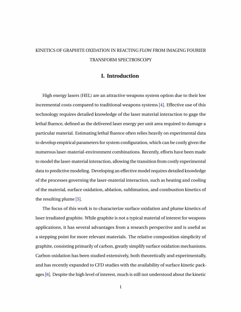
High energy lasers (HEL) are an attractive weapons system option due to their low
incremental costs compared to traditional weapons systems [4]. Effective use of this
technology requires detailed knowledge of the laser material interaction to gage the
lethal fluence, defined as the delivered laser energy per unit area required to damage a
particular material. Estimating lethal fluence often relies heavily on experimental data
to develop empirical parameters for system configuration, which can be costly given the
numerous laser-material-environment combinations. Recently, efforts have been made
to model the laser-material interaction, allowing the transition from costly experimental
data to predictive modeling. Developing an effective model requires detailed knowledge
of the processes governing the laser-material interaction, such as heating and cooling
of the material, surface oxidation, ablation, sublimation, and combustion kinetics of
the resulting plume [5].
The focus of this work is to characterize surface oxidation and plume kinetics of
laser irradiated graphite. While graphite is not a typical material of interest for weapons
applications, it has several advantages from a research perspective and is useful as
a stepping point for more relevant materials. The relative composition simplicity of
graphite, consisting primarily of carbon, greatly simplify surface oxidation mechanisms.
Carbon oxidation has been studied extensively, both theoretically and experimentally,
and has recently expanded to CFD studies with the availability of surface kinetic pack-
ages [6]. Despite the high level of interest, much is still not understood about the kinetic
1
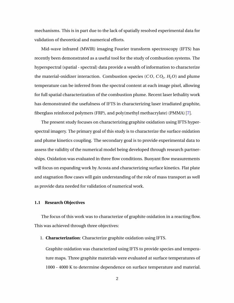
mechanisms. This is in part due to the lack of spatially resolved experimental data for
validation of theoretical and numerical efforts.
Mid-wave infrared (MWIR) imaging Fourier transform spectroscopy (IFTS) has
recently been demonstrated as a useful tool for the study of combustion systems. The
hyperspectral (spatial - spectral) data provide a wealth of information to characterize
the material-oxidizer interaction. Combustion species (C O , C O2, H2O ) and plume
temperature can be inferred from the spectral content at each image pixel, allowing
for full spatial characterization of the combustion plume. Recent laser lethality work
has demonstrated the usefulness of IFTS in characterizing laser irradiated graphite,
fiberglass reinforced polymers (FRP), and poly(methyl methacrylate) (PMMA) [7].
The present study focuses on characterizing graphite oxidation using IFTS hyper-
spectral imagery. The primary goal of this study is to characterize the surface oxidation
and plume kinetics coupling. The secondary goal is to provide experimental data to
assess the validity of the numerical model being developed through research partner-
ships. Oxidation was evaluated in three flow conditions. Buoyant flow measurements
will focus on expanding work by Acosta and characterizing surface kinetics. Flat plate
and stagnation flow cases will gain understanding of the role of mass transport as well
as provide data needed for validation of numerical work.
1.1 Research Objectives
The focus of this work was to characterize of graphite oxidation in a reacting flow.
This was achieved through three objectives:
1. Characterization: Characterize graphite oxidation using IFTS.
Graphite oxidation was characterized using IFTS to provide species and tempera-
ture maps. Three graphite materials were evaluated at surface temperatures of
1000 - 4000 K to determine dependence on surface temperature and material.
2
Plume properties and surface temperature were inferred from IFTS and MW ther-
mal imagery, respectively. Three flow conditions were evaluated to highlight the
role of transport mechanisms: buoyant flow (Chapter IV), flat plate shear flow
(Chapter V), and stagnation flow (Chapter VI). Differences in oxidation plumes
and [C O ]/C O2] product ratios for each flow condition are discussed.
Two techniques were developed to infer diffusion and convective transport prop-
erties from IFTS data. Diffusion transport is estimated using species gradients
inferred from 2D species maps. Convective transport is characterized through
visualization of the velocity flow field. Velocity fields are estimated using the
cross-correlation of low frequency signal oscillations in neighboring pixels to
estimate the flow travel time. Repeating across the array then gives a full spatial
flow velocity map, enabling visualization of convective transport.
2. Modeling: Develop an oxidation model incorporating transport and kinetics.
While ideally the oxidation process would be modeled using CFD coupled with
kinetic packages, these methods are computationally expensive and lack the
simplicity to develop intuition. Two simplified models were developed to gain
intuition on the role of transport and kinetic mechanisms.
A simple 1D model based on previous theoretical work is presented. A system
of ordinary differential equations (ODEs) is derived from species and energy
conservation equations incorporating surface and gas phase kinetics and diffusion
transport (neglecting convection). A numerical boundary value solver is used to
determine species concentration and temperature normal to the surface. Results
are in general agreement with trends reported experimentally. Derivation of the
model and sample simulations are presented in Chapter III.
A quasi 2D model was then developed to incorporate kinetics, diffusion transport
3
(normal to surface), and convective transport (along surface). Species and energy
conservations are applied to a small control volume adjacent to the surface. Ap-
proximations to diffusion transport are applied to simplify the system of equations
to a set of ODEs. A numerical solver is then used to determine species concentra-
tion and temperature along the surface. Trends are in general agreement those
observed experimentally. Derivation of the model is presented in Chapter III.
Model results are compared with experimental observations in Chapters IV and V.
3. CFD Validation: Provide experimental data for validation of numerical results.
A research partnership has been established with the University of Virginia (UVa)
to aid in the numerical modeling of the surface and plume oxidation [8]. Numeri-
cal simulations of high temperature graphite oxidation in stagnation and flat plate
flow have been completed. The experimental work was designed to compliment
numerical efforts and provide data for validation. Experimental results provide
the first sub-mm resolved measurements of graphite oxidation in reacting flow
(both flat plate and stagnation). Unfortunately, we were unable to match experi-
mental conditions to existing simulations, but this work will provide valuable data
for validation of future CFD efforts. This objective is met though the flat plate and
stagnation flow data found in Chapters V and VI. Additional data can be found in
Appendix A.
1.2 Document Outline
An outline of the document is presented to highlight the document organization and
the material presented in each chapter. Chapter II provides a more in depth coverage
of the relevant background material, including a review of carbon oxidation kinetics
and an introduction to IFTS and its application as a combustion diagnostic. Chapter III
presents the two oxidation models, including their derivation and simulation trends.
4

Each of the central chapters (IV, V, VI) represent experimental work in each of the
three flow conditions evaluated: buoyant, flat plate shear flow, and stagnation flow,
respectively. Each central chapter is intended for submission to publication and can
be read as a stand alone document. Supplemental data and figures for the three flow
conditions can be found in Appendix A. Finally, conclusions and recommendations for
future work can be found in Chapter VII.
5
II. Background
2.1 Summary
This chapter provides a review of the basic concepts needed to describe graphite
oxidation and the diagnostics used in this study. Section 2.2 covers the basics of carbon
oxidation, the mechanisms involved, and a review of previous experimental work. Sec-
tion 2.3 includes an introduction to Fourier transform spectroscopy, which is primary
diagnostic used in this study. Lasty, Section 2.4 provides background for each of the
flow configurations used in this study, including basic fluid equations.
2.2 Carbon Oxidation
Overview.
Extensive research on carbon oxidation has been done due to its applications in
coal/char combustion [9–11]. Despite numerous studies, much of the kinetics is still not
well understood. The main source of complexity in carbon oxidation is the coupling of
heterogeneous and homogeneous reactions, which make it difficult to measure surface
mechanisms independently. A graphic summary of the reacting system is shown in
Figure 1. Oxidizing species (O2, C O2) diffuse to the surface and react with carbon,
producing C O and C O2 through S1, S2, and S3:
S1) 2Cs +O2 =⇒ 2C O (1)
S2) Cs +C O2 =⇒ 2C O (2)
S3) Cs +O2 =⇒ C O2 (3)
6
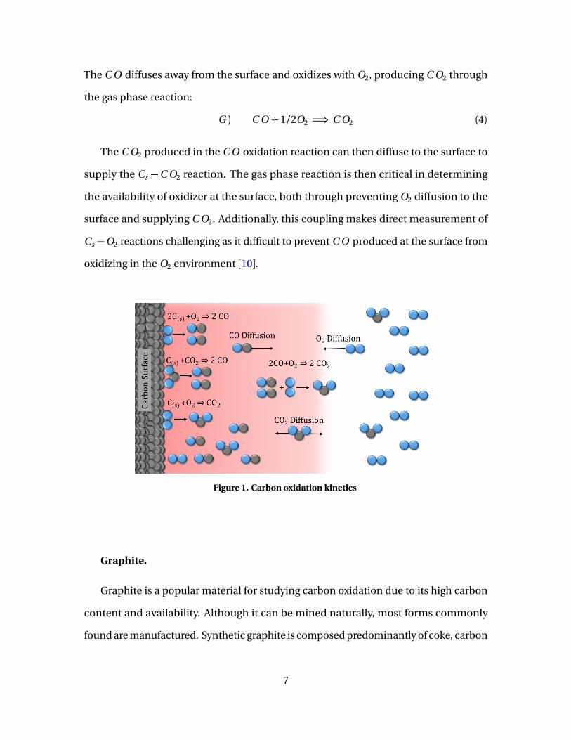
The C O diffuses away from the surface and oxidizes with O2, producing C O2 through
the gas phase reaction:
G ) C O +1/2O2 =⇒ C O2 (4)
The C O2 produced in the C O oxidation reaction can then diffuse to the surface to
supply the Cs −C O2 reaction. The gas phase reaction is then critical in determining
the availability of oxidizer at the surface, both through preventing O2 diffusion to the
surface and supplying C O2. Additionally, this coupling makes direct measurement of
Cs −O2 reactions challenging as it difficult to prevent C O produced at the surface from
oxidizing in the O2 environment [10].
Figure 1. Carbon oxidation kinetics
Graphite.
Graphite is a popular material for studying carbon oxidation due to its high carbon
content and availability. Although it can be mined naturally, most forms commonly
found are manufactured. Synthetic graphite is composed predominantly of coke, carbon
7
black, natural graphite, and binder [12]. The coke, carbon black, and graphite are ground
into a powder and held together with a coal, petroleum, or resin based binder. The
mixture is then shaped, typically using isostatic press, extrusion, or die molding. Heat
treatment varies, but typically involves at least two stages. In the first stage, the formed
mixture is slowly heated in vacuum to remove any volatiles which may be present in
the binder. A filler material may be used to fill the voids left by the escaped volatiles. In
the second stage, the material is heated treated (T ≈ 3300 K) which helps graphitize the
material and remove any remaining volatiles and impurities. As a result of variation in
these production steps, graphite materials often vary in porosity and impurity content,
which can result in some variation in surface reactivity.
CO Oxidation.
Oxidation of C O has been widely studied due to its application in most combustion
processes. While C O oxidation is written simply as the global reaction in Eq. (4), in
reality it consists of many elementary reactions between C O , C O2, O2,and H2O as well
as their radicals (O H , H , O , etc). H2O is critical in to the production of H and O H
radicals which control propagating and branching reactions [13]. Extensive research
has been done to develop kinetic packages consisting of a finite number of elementary
reactions, while still adequately characterizing C O oxidation over a range of conditions.
For example, the model proposed by Yetter et al. consists of 28 elementary reactions
between 12 species [13].
For simplicity, it is often desired to use a single step global reaction with empirical
coefficients, typically expressed as [14]:
Rg = [C O ][O2]a [H2O ]b ·Ag e x p
�
−Eg
RTp
�
(5)
where Rg is the gas phase oxidation rate in mol/m3/s, [Ci ] is the concentration of
8
species Ci in mol/m3, and Ag e x p (−Eg
RTp) is the Arrhenius rate coefficient, kg , with pre-
exponential factor Ag in (mol/m3)-(a+b)/s, activation energy Eg in kcal/mol, and universal
gas constant R . The [H2O ]b term is added to incorporate the influence of H2O and its
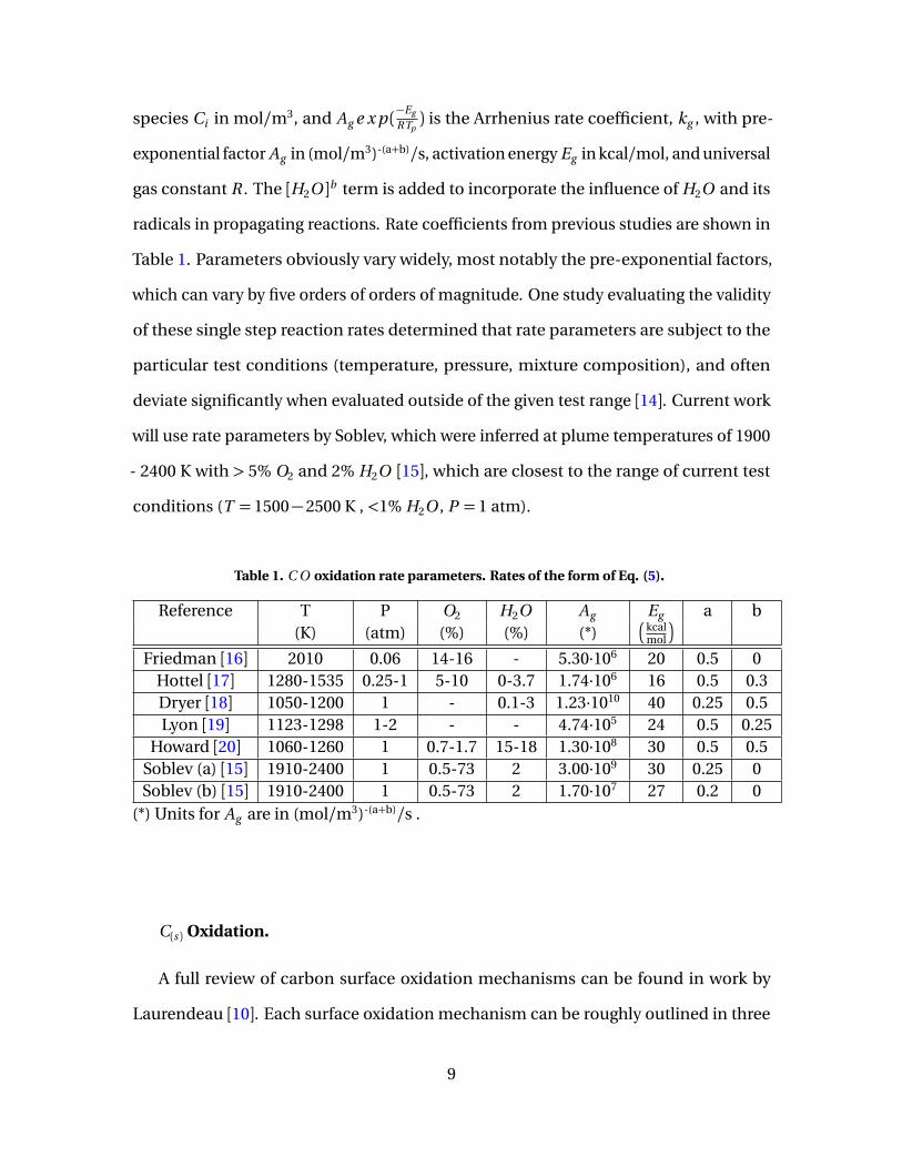
radicals in propagating reactions. Rate coefficients from previous studies are shown in
Table 1. Parameters obviously vary widely, most notably the pre-exponential factors,
which can vary by five orders of orders of magnitude. One study evaluating the validity
of these single step reaction rates determined that rate parameters are subject to the
particular test conditions (temperature, pressure, mixture composition), and often
deviate significantly when evaluated outside of the given test range [14]. Current work
will use rate parameters by Soblev, which were inferred at plume temperatures of 1900
- 2400 K with > 5% O2 and 2% H2O [15], which are closest to the range of current test
conditions (T = 1500−2500 K , <1% H2O , P = 1 atm).
Table 1. C O oxidation rate parameters. Rates of the form of Eq. (5).
Reference T P O2 H2O Ag Eg a b(K) (atm) (%) (%) (*)
�
kcalmol
�
Friedman [16] 2010 0.06 14-16 - 5.30·106 20 0.5 0Hottel [17] 1280-1535 0.25-1 5-10 0-3.7 1.74·106 16 0.5 0.3Dryer [18] 1050-1200 1 - 0.1-3 1.23·1010 40 0.25 0.5Lyon [19] 1123-1298 1-2 - - 4.74·105 24 0.5 0.25
Howard [20] 1060-1260 1 0.7-1.7 15-18 1.30·108 30 0.5 0.5Soblev (a) [15] 1910-2400 1 0.5-73 2 3.00·109 30 0.25 0Soblev (b) [15] 1910-2400 1 0.5-73 2 1.70·107 27 0.2 0
(*) Units for Ag are in (mol/m3)-(a+b)/s .
C(s ) Oxidation.
A full review of carbon surface oxidation mechanisms can be found in work by
Laurendeau [10]. Each surface oxidation mechanism can be roughly outlined in three
9
steps: 1) oxidizer adsorption to produce active sites, 2) migration of active sites, and 3)
desorption of products. These steps for the Cs −C O2 surface reaction given by Eq. (2)
can be written as follows:
C O2+Cs− f =⇒ C (O )∗+C O (6)
C (O )∗ =⇒ C (O )∗′
(7)
C (O )∗′=⇒ C O (8)
where Cs− f represents a free carbon site, and C (O )∗ and C (O )∗′ represent two active sites
[10]. The simplest kinetic model of this system is the Langmuir-Hinshelwood model,
which relies on three main assumptions: instantaneous migration, no interaction of
adsorbed species, and a uniform reacting surface. Using these assumptions, the rates
of adsorption and desorption can then be written as:
Ra = ka [Co x ]θζf (9)
Rd = kd (1−θ f )ζ (10)
where ka and kd are the adsorption and desorption rate coefficients in Arrhenius form,
[Co x ] is the oxidizer concentration, θ f is the fraction of free carbon sites, and ζ refers to
single (ζ= 1) or dual (ζ= 2) site interactions. Assuming equilibrium, Ra =Rd =Rs , and
single site interactions (ζ= 1), yields the surface reaction rate:
Rs = ka
[Co x ]1+a [Co x ]
(11)
a =Aa
Ade x p (
Ed −Ea
RT) (12)
10
where Ai and Ei are the pre-exponential factors and activation energies for adsorption
and desorption. Evaluation of Eq. (11) for the two extremes of a [Co x ] yields the first
and zero order expressions:
Rs =
ka [Co x ] a [Co x ]� 1
kd /a a [Co x ]� 1
(13)
Global reaction rates for each surface oxidation mechanism are therefore typically
expressed using the form :
Rs = ks [Co x ]m (14)
with reaction order 0<m < 1.
The limits of the Langmuir-Hinshelwood model assumptions are discussed in detail
by Laurendeau [10]. First, take the assumption of no interaction of adsorbed species.
Measurements have shown that both Ea and Ed are influenced by the fraction of ac-
tive sites, θs = 1− θ f . For the adsorption process, as more sites become active, the
more repulsive the surface becomes to potential adsorbed species, increasing the ac-
tivation energy. For desorption, the process is reversed, with desorption activation
energy decreasing with increasing reactivity. The simplest modification to reflect these
observations is a simple linear correction:
Ea = Ea 0+ωaθs (15)
Ed = Ed 0−ωdθs (16)
whereωa andωd describe the degree of influence of active sites. The second assumption
of a uniform reacting surface implies a single activation energy. However, experimental
work has already shown activation energies to exhibit a Gaussian distribution [21].
11

Despite these limitations Eq. (14) remains the most popular expression for surface
kinetics due to its simplicity.
Measurements of the surface oxidation rates are difficult due to the coupling of
the surface and gas phase reactions. This is particularly problematic in Cs −O2 mea-
surements where the available O2 can further oxidize surface products and influence
measurements. For techniques where the gas is captured and analyzed, the O2 in the
mixture can quickly oxidize C O , creating C O2 before the gas sample is analyzed. It is
therefore difficult to determine if observed C O2 was created through surface production
or C O oxidation [22, 23]. This has led to much debate over the S3 reaction. Although
spatially resolved techniques, such as IFTS, can vastly improve our understanding of
these surface mechanisms, there is still room for false interpretation of surface C O2.
C O produced through S1 and S2, either at the surface or within the pores, can easily
be oxidized at the surface given a significant O2 population, producing a high surface
C O2 which can falsely interpreted as the S3 reaction.
Reactions considered for this study are shown in Table 2, which consider only Cs −
C O2 and Cs −O2 reactions. Much work has been done on the Cs −C O2 interactions
[24–30]. Most debated about this reaction is the inhibition of the S2 reaction by C O ,
which has been noted in experimental work. Gadsby proposed this is result of C O
occupation of active sites, preventing C O2 absorption [26]. Ergun however believed this
to be a result of C O reacting with C (O ) produced in the intermediate steps [24, 25]. In
either case, a more complex form of the S2 reaction rate is derived, taking into account
these elementary steps. However for simplicity, a first order Arrhenius expression, as
given in Eq. (14), is often desired. Large variation is seen in pre-exponential factors and
activation energies vary across literature, with reported Ei values ranging from 24,000 -
43,000 K.
Cs −O2 reactions are much more difficult to characterize [10]. Central to this issue is
12
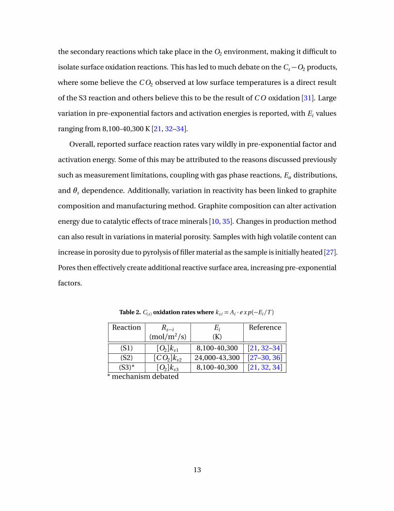
the secondary reactions which take place in the O2 environment, making it difficult to
isolate surface oxidation reactions. This has led to much debate on the Cs −O2 products,
where some believe the C O2 observed at low surface temperatures is a direct result
of the S3 reaction and others believe this to be the result of C O oxidation [31]. Large
variation in pre-exponential factors and activation energies is reported, with Ei values
ranging from 8,100-40,300 K [21, 32–34].
Overall, reported surface reaction rates vary wildly in pre-exponential factor and
activation energy. Some of this may be attributed to the reasons discussed previously
such as measurement limitations, coupling with gas phase reactions, Ea distributions,
and θs dependence. Additionally, variation in reactivity has been linked to graphite
composition and manufacturing method. Graphite composition can alter activation
energy due to catalytic effects of trace minerals [10, 35]. Changes in production method
can also result in variations in material porosity. Samples with high volatile content can
increase in porosity due to pyrolysis of filler material as the sample is initially heated [27].
Pores then effectively create additional reactive surface area, increasing pre-exponential
factors.
Table 2. C(s ) oxidation rates where ks i = Ai · e x p (−Ei /T )
Reaction Rs−i Ei Reference(mol/m2/s) (K)
(S1) [O2]ks 1 8,100-40,300 [21, 32–34](S2) [C O2]ks 2 24,000-43,300 [27–30, 36](S3)* [O2]ks 3 8,100-40,300 [21, 32, 34]
* mechanism debated
13
[C O ]/[C O2] Temperature Dependence.
Numerous studies on carbon oxidation have been completed to date. Plots of
[C O ]/[C O2] versus T became popular to describe the oxidation process. In 1951, Arthur
investigated carbon oxidation at low temperature (730 - 1170 K) using POCl3 to suppress
C O oxidation and isolate the effects from surface kinetics [37]. Two carbon materials
were evaluated, an artificial graphite and coal char, to determine variation in reactivity
between carbon materials. The reacted gases were then fed to a Haldane apparatus
to determine C O , C O2, and O2. [C O ]/[C O2] for the two carbon materials showed an
exponential dependence on temperature, establishing the following expression:
[C O ][C O2]
= 2500 exp�
−6, 240
T
�
(17)
Future carbon oxidation work continued to report data in terms of [C O ]/[C O2] ex-
pressed in Arrhenius form:
[C O ][C O2]
=α · [O2]n exp
�
−β
T
�
(18)
where α, β , and n are determined through fitting of experimental data. A summary of
experimental studies is shown in Table 3. Much of the work was originally done using
gas sampling techniques, such as mass spectrometers [21, 39–41, 89]. However this can
lead to lower C O/C O2 ratios as C O can further evolve into C O2 given the time between
sampling and analyzing. The more recent work by Acosta presented the first spatially
resolved measurements of carbon oxidation using IFTS [1]. This technique shows much
improvement over gas sampling techniques due to the ability to isolate species located
directly adjacent to the surface. However, reported β values are significantly higher
than those in earlier literature, possibly due to measurements being taken during the
transient heating period and not purely during steady state.
14
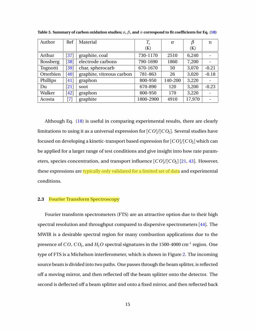
Table 3. Summary of carbon oxidation studies; α, β , and n correspond to fit coefficients for Eq. (18)
Author Ref Material Ts α β n(K) (K)
Arthur [37] graphite, coal 730-1170 2510 6,240 -Rossberg [38] electrode carbons 790-1690 1860 7,200 -Tognotti [39] char, spherocarb 670-1670 50 3,070 -0.21Otterbien [40] graphite, vitreous carbon 781-863 26 3,020 -0.18Phillips [41] graphon 800-950 140-200 3,220 -Du [21] soot 670-890 120 3,200 -0.23Walker [42] graphon 800-950 170 3,220 -Acosta [7] graphite 1800-2900 4910 17,970 -
Although Eq. (18) is useful in comparing experimental results, there are clearly
limitations to using it as a universal expression for [C O ]/[C O2]. Several studies have
focused on developing a kinetic-transport based expression for [C O ]/[C O2]which can
be applied for a larger range of test conditions and give insight into how rate param-
eters, species concentration, and transport influence [C O ]/[C O2] [21, 43]. However,
these expressions are typically only validated for a limited set of data and experimental
conditions.
2.3 Fourier Transform Spectroscopy
Fourier transform spectrometers (FTS) are an attractive option due to their high
spectral resolution and throughput compared to dispersive spectrometers [44]. The
MWIR is a desirable spectral region for many combustion applications due to the
presence of C O , C O2, and H2O spectral signatures in the 1500-4000 cm-1 region. One
type of FTS is a Michelson interferometer, which is shown in Figure 2. The incoming
source beam is divided into two paths. One passes through the beam splitter, is reflected
off a moving mirror, and then reflected off the beam splitter onto the detector. The
second is deflected off a beam splitter and onto a fixed mirror, and then reflected back
15
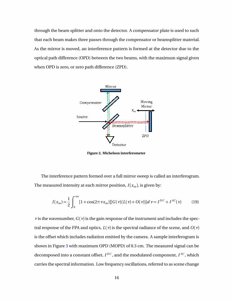
through the beam splitter and onto the detector. A compensator plate is used to such
that each beam makes three passes through the compensator or beamsplitter material.
As the mirror is moved, an interference pattern is formed at the detector due to the
optical path difference (OPD) between the two beams, with the maximum signal given
when OPD is zero, or zero path difference (ZPD).
Figure 2. Michelson interferometer
The interference pattern formed over a full mirror sweep is called an interferogram.
The measured intensity at each mirror position, I (xm ), is given by:
I (xm ) =1
2
∫ ∞
0
[1+ cos(2πνxm )][G (ν) (L (ν) +O (ν))]dν= I D C + I AC (ν) (19)
ν is the wavenumber, G (ν) is the gain response of the instrument and includes the spec-
tral response of the FPA and optics, L (ν) is the spectral radiance of the scene, and O (ν)
is the offset which includes radiation emitted by the camera. A sample interferogram is
shown in Figure 3 with maximum OPD (MOPD) of 0.3 cm. The measured signal can be
decomposed into a constant offset, I D C , and the modulated component, I AC , which
carries the spectral information. Low frequency oscillations, referred to as scene change
16

artifacts (SCA), are sometimes observed in the I D C component. These are below the
cut-off frequency of the interference modulation and are attributed to oscillations in
the scene[45].
Figure 3. Sample interferogram, MOPD = 0.3 cm, nOPD = 9480
The uncalibrated spectrum is then produced by taking the fast Fourier transform
(FFT) of the interferogram:
Y (ν) =F [I (xm )] (20)
The calibrated spectrum is then calculated using Y (ν) and the characterized instrument
response:
L (ν) =Y (ν)G (ν)
−O (ν) (21)
where gain and offset are determined using a blackbody calibration procedure described
in Chapter IV.
17
Radiative Transfer Model.
A radiative transfer model (RTM) is used to infer plume properties from the measured
spectra. The simplest RTM is the single layer model where the measured spectral
radiance is expressed as:
L = ε(α)B (T ) (22)
where B (T ) is the blackbody spectral radiance at temperature T , and emissivity, ε, is
defined in terms of optical depth α as:
ε = 1− e x p (−α) (23)
Optical depth is determined by the flame composition and can be expressed as:
α= n`∑
i
X iσi (ν, T ) (24)
where n is concentration, ` is path length, X i is the mole fraction of species i , and
σi is the cross-section of species i at temperature T . Cross-sections are provided for
common combustion species by spectral databases, such as HITRAN or CDSD [46, 47].
Most systems however require at the very least a two layer RTM. In this case, the two
layers consist of the flame layer and the atmospheric layer between the flame and the
detector. The measured radiance can be expressed as:
Ld e t =τa t mo s Lp l ume + La t mo s (25)
where Lp l ume and La t mo s are the plume and path radiance defined similarly by Eq. (22),
and path transmissivity, τa t mo s is expressed as:
τa t mo s = 1− εa t mo s (n , X i−a t mo s , Ta t mo s ,`a t mo s ) (26)
18
For typical combustion applications La t mo s is neglected (La t mo s � Lp l ume ). The mea-
sured radiance is then expressed as:
Ld e t =τa t mo s · εp l ume ·B (Tp l ume ) (27)
A nonlinear fit routine is used to determine plume and atmospheric values for X i and
temperature.
2.4 Flow Conditions
Graphite oxidation is evaluated in three flow conditions: buoyant flow, flat plate
shear flow, and stagnation flow. For non-reacting flow, each of these flow conditions
has been well studied, both theoretically and experimentally. An overview of each flow
configuration, including the basic governing equations, is provided in the following
sections.
Flat Plate Shear Flow.
One of the most commonly evaluated forced flow problems is the flat plate shear
flow, also known as flat plate in a parallel flow, as shown in Figure 4. This case considers
a uniform freestream velocity, u∞, incident on a flat plate with uniform temperature
Ts . A boundary layer is formed between the no-slip condition imposed by the wall,
u (y = 0) = 0, and the freestream velocity u (y →∞) = u∞. Similarly, a thermal boundary
layer is also formed due to the temperature gradient. This problem has been studied
extensively to determine expressions for boundary layer and thermal boundary layer
thickness.
19
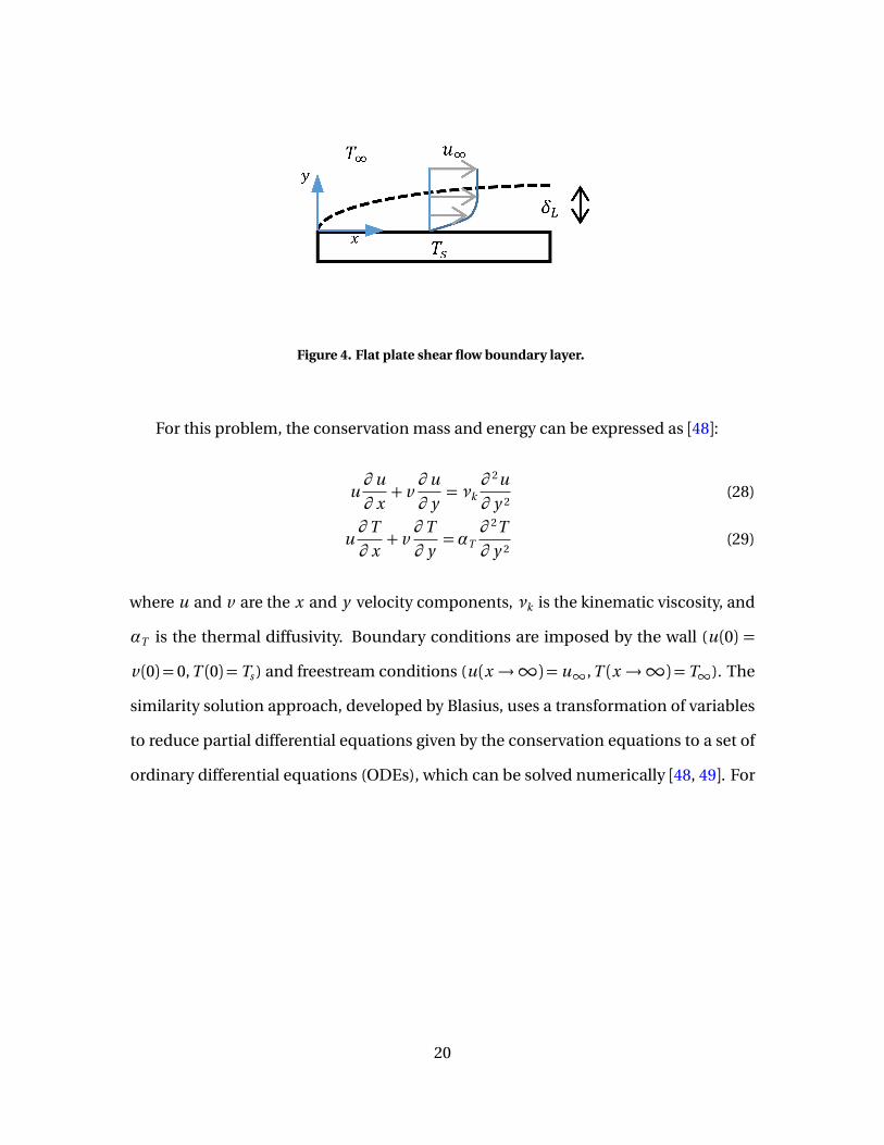
Figure 4. Flat plate shear flow boundary layer.
For this problem, the conservation mass and energy can be expressed as [48]:
u∂ u
∂ x+ v∂ u
∂ y= νk
∂ 2u
∂ y 2(28)
u∂ T
∂ x+ v∂ T
∂ y=αT
∂ 2T
∂ y 2(29)
where u and v are the x and y velocity components, νk is the kinematic viscosity, and
αT is the thermal diffusivity. Boundary conditions are imposed by the wall (u (0) =
v (0) = 0, T (0) = Ts ) and freestream conditions (u (x →∞) = u∞, T (x →∞) = T∞). The
similarity solution approach, developed by Blasius, uses a transformation of variables
to reduce partial differential equations given by the conservation equations to a set of
ordinary differential equations (ODEs), which can be solved numerically [48, 49]. For
20
the flat plate case, the following variable substitutions are used:
u =∂ ψ
∂ y(30)
v =−∂ ψ
∂ x(31)
η= y
√
√ u∞νv x
(32)
ψ= f (η)
�
u∞
√
√νv x
u∞
�
(33)
θT =T −Ts
T∞−Ts(34)
Eq. (28) and (29) can then be written as:
2 f ′′′+ f f ′′ = 0 (35)
θ ′′T +Pr
2f θ ′T = 1 (36)
where Pr is the Prandtl number defined as the ratio of momentum and thermal diffusiv-
ities:
Pr=νv
αT(37)
Eq. (35) and (36) can be solved numerically with the following converted boundary
conditions:
u (y = 0) = 0 f ′(η= 0) = 0 (38)
u (y →∞) = u∞ f ′(η→∞) = 1 (39)
v (y = 0) = 0 f (η= 0) = 0 (40)
T (y = 0) = Ts θT (η= 0) = 0 (41)
T (y →∞) = T∞ θT (η→∞) = 1 (42)
21
Solutions for f , f ′,θT , and θ ′T can then be used to infer properties of the flow. For
instance, f ′ gives the velocity profile:
f ′(η) =u
u∞(43)
The boundary layer is then defined as the point where u = 0.99u∞, which corresponds
to η= 5. Using Eq. (32), boundary layer thickness can be expressed as:
δ=5x
p
Rex
(44)
where Reynolds number, Rex , is defined as [48]:
Rex =u∞x
νk(45)
A similar expression for thermal boundary layer is also developed:
δT =δPr−1/3 (46)
Buoyant Flow.
In the case of buoyant flow, fluid motion is due to density gradients within the
fluid and the gravitational body force. These combine to produce what is referred to
as free convection flow. One of the most studied problems in free convection flow is
the isothermal vertical flat plate in a quiescent environment. As depicted in Figure
5, this problem consists of a vertical flat plate with surface temperatures higher than
the environment (Ts > T∞). The temperature difference produces a thermal gradient,
which results in a density gradient with the heated fluid near the surface being forced
upward. The velocity distribution is then dictated by the temperature gradient, with
22
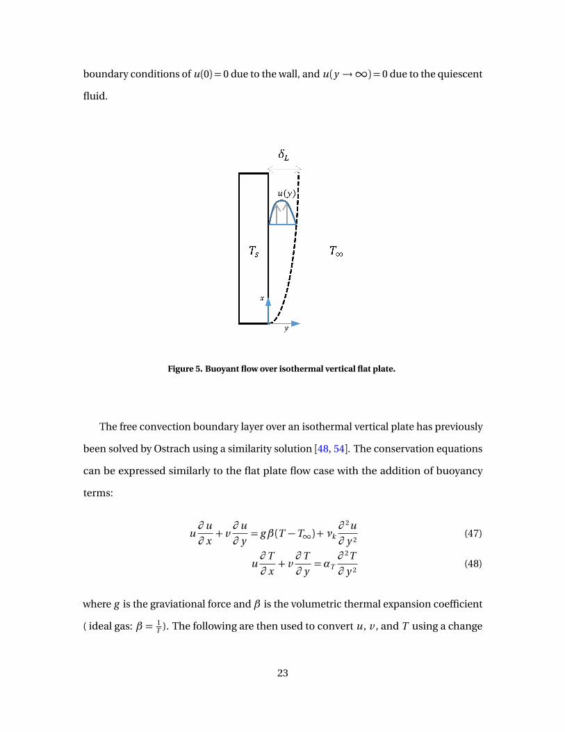
boundary conditions of u (0) = 0 due to the wall, and u (y →∞) = 0 due to the quiescent
fluid.
Figure 5. Buoyant flow over isothermal vertical flat plate.
The free convection boundary layer over an isothermal vertical plate has previously
been solved by Ostrach using a similarity solution [48, 54]. The conservation equations
can be expressed similarly to the flat plate flow case with the addition of buoyancy
terms:
u∂ u
∂ x+ v∂ u
∂ y= gβ (T −T∞) +νk
∂ 2u
∂ y 2(47)
u∂ T
∂ x+ v∂ T
∂ y=αT
∂ 2T
∂ y 2(48)
where g is the graviational force and β is the volumetric thermal expansion coefficient
( ideal gas: β = 1T ). The following are then used to convert u , v , and T using a change
23
of variables:
u =∂ ψ
∂ y(49)
v =−∂ ψ
∂ x(50)
η=y
x
�
Grx
4
�1/4
(51)
ψ= f (η)
�
4νv
�
Grx
4
�1/4�
(52)
θT =T −T∞Ts −T∞
(53)
where Grx is the Grashof number which measures the ratio of buoyancy to viscous
forces [48]:
G rx =gβ (Ts −T∞)x 3
ν2v
(54)
Eq. (47) and (48) can then be written as:
f ′′′+3 f f ′′−2( f ′)2+θT = 0 (55)
θ ′′T +3Pr f θ ′T = 0 (56)
The boundary conditions are then transformed using the change of variables:
u (y = 0) = 0 f ′(η= 0) = 0 (57)
u (y →∞) = 0 f ′(η→∞) = 0 (58)
v (y = 0) = 0 f (η= 0) = 0 (59)
T (y = 0) = Ts θT (η= 0) = 1 (60)
T (y →∞) = T∞ θT (η→∞) = 0 (61)
This set of ODEs and boundary conditions can then be solved numerically for f and θT .
24
Using these solutions, boundary layer thickness, δ, for free convection flow along a
vertical plate can be approximated for Pr= 0.7 in terms of Gr as [48]:
δx ≈6x
(Gr/4)1/4(62)
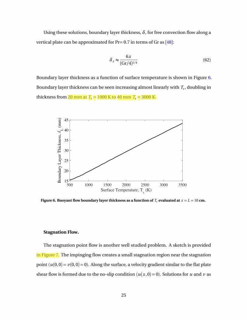
Boundary layer thickness as a function of surface temperature is shown in Figure 6.
Boundary layer thickness can be seen increasing almost linearly with Ts , doubling in
thickness from 20 mm at Ts = 1000 K to 40 mm Ts = 3000 K.
500 1000 1500 2000 2500 3000 3500Surface Temperature, Ts (K)
15
20
25
30
35
40
45
Boun
dary
Lay
er T
hick
ness
, δL (m
m)
Figure 6. Buoyant flow boundary layer thickness as a function of Ts evaluated at x = L = 10 cm.
Stagnation Flow.
The stagnation point flow is another well studied problem. A sketch is provided
in Figure 7. The impinging flow creates a small stagnation region near the stagnation
point (u (0, 0) = v (0, 0) = 0). Along the surface, a velocity gradient similar to the flat plate
shear flow is formed due to the no-slip condition (u (x , 0) = 0). Solutions for u and v as
25
a function of location are derived using similarity solutions as with the flat plate shear
flow case. Using the following variable substitutions the flow can be described using a
set of solvable ODEs [50, 51]:
u =∂ ψ
∂ y(63)
v =−∂ ψ
∂ x(64)
η= y
√
√ B
νv(65)
ψ= x f (η)p
Bνv (66)
θT =T −Ts
T∞−Ts(67)
where B is the stagnation velocity gradient, which is generally proportional to u∞/L
where u∞ is the freestream flow velocity and L is a characteristic length [52]. For a 3D
axisymmetric stagnation flow, B = 3u∞/L . The conservation equations can then be
written as:
f ′′′+ f f ′′+1− f ′2 = 0 (68)
θ ′′T +Pr f θ ′T = 0 (69)
with boundary conditions:
u (y = 0) = 0 f ′(η= 0) = 0 (70)
v (y = 0) = 0 f (η= 0) = 0 (71)
u (y →∞) = B x f ′(η→∞) = 1 (72)
T (y = 0) = Ts θT (η= 0) = 0 (73)
T (y →∞) = T∞ θT (η→∞) = 1 (74)
26
The ODEs and boundary conditions can be solved using a numerical boundary value
solver.
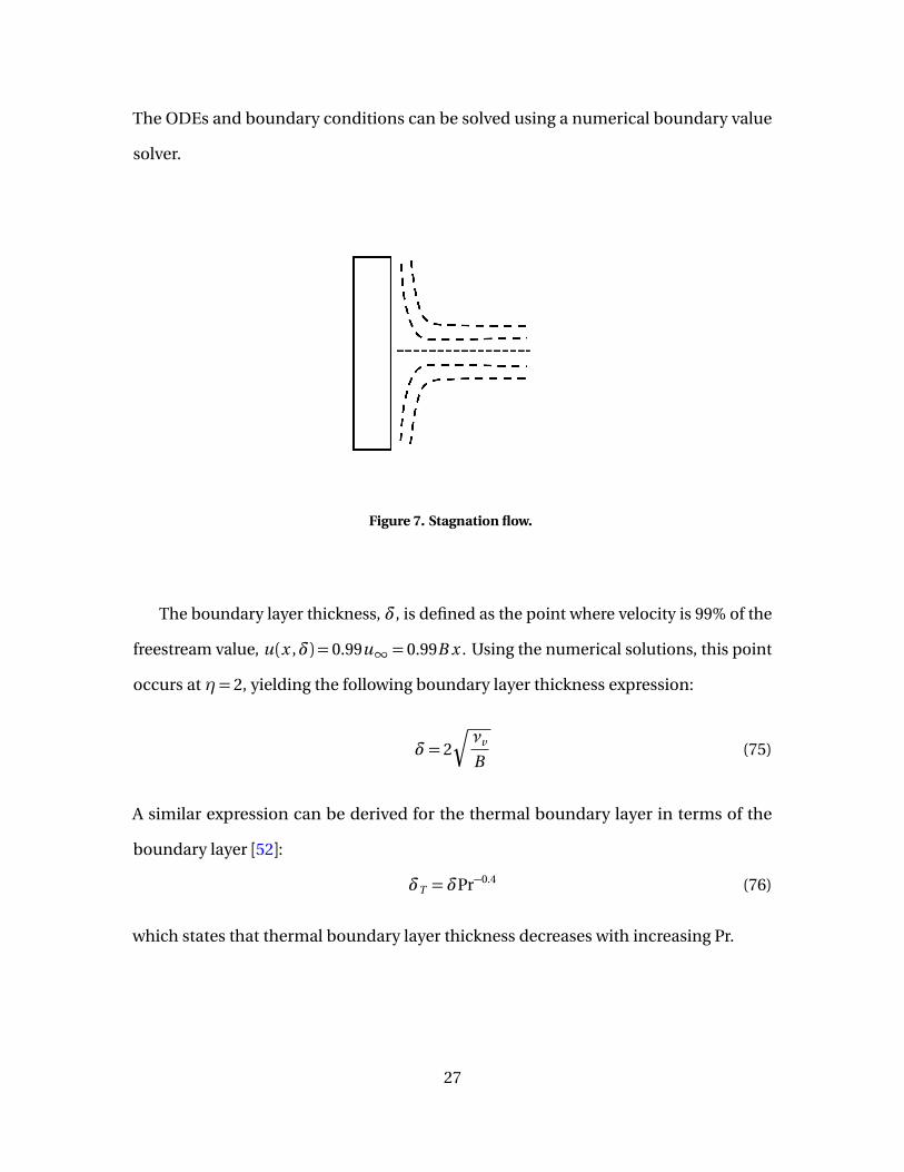
Figure 7. Stagnation flow.
The boundary layer thickness, δ, is defined as the point where velocity is 99% of the
freestream value, u (x ,δ) = 0.99u∞ = 0.99B x . Using the numerical solutions, this point
occurs at η= 2, yielding the following boundary layer thickness expression:
δ= 2
s
νv
B(75)
A similar expression can be derived for the thermal boundary layer in terms of the
boundary layer [52]:
δT =δPr−0.4 (76)
which states that thermal boundary layer thickness decreases with increasing Pr.
27

III. Oxidation Model
This chapter provides detail regarding modeling of the carbon oxidation process. A
review of the conservation equations and relevant terms is provided in Section 3.1. Two
simplified oxidation models are then presented. The first, presented in Section 3.2, is a
1D diffusion - kinetics model used to evaluate properties normal to the surface. The
second, presented in Section 3.3, is a quasi 2D model incorporating diffusion (normal to
the surface) and convection (along surface) and is used to evaluate properties along the
surface. While both models have significant limitations due to their assumptions, they
are useful in gaining intuition about the problem and interpreting experimental obser-
vations. Comparison of simulations with experimental data is discussed in Chapter V -
VI
3.1 Conservation Equations
The species conservation equation is expressed as:
d Ci
d t=ωi − v ·∇Ci +∇·Di∇Ci (77)
where Ci is the concentration of species i ,ωi is the reaction source term, v ·∇Ci is the
convective transport term with velocity vector v , and∇·Di∇Ci is the diffusion transport
term with Di as diffusion coefficient of species i . Similarly the conservation of energy,
neglecting diffusion thermal transport, can be expressed as:
dρh
d t= q − v ·∇ρh +∇·αT∇ρh (78)
28
where h is the sensible enthalpy, q is the source term due to the gas phase reactions,
ρ is the gas denisty, and αT is the thermal resistivity. . The enthalpy term can be
approximated in terms of specfic heat Cp as h ≈Cp T .
Assuming steady state and a uniform gas (ρ, cp and D constant), Eq. (77) and (78)
can then be written as:
−D∇2Ci =ωi − v ·∇Ci (79)
−λ∇2T = q − vρcp ·∇T (80)
where λ is the thermal conductivity (λ=αTρcp ).
3.2 1D Model
We first consider the 1D case with the reactive surface at y = 0. Heterogeneous
reactions take place at the surface boundary and homogeneous reactions within the
gas (y > 0). Flow normal to the surface is neglected (vy = 0). Rewriting Eq. (79) for the
1D case:
−D C ′′i =ωi (81)
where C ′′i refers to the second derivative normal to the surface. The convection term is
neglected due to the assumption of zero velocity normal to the surface. Applying this
to the three species of interest, and substituting the gas phase rate equation (Eq. (5),
a = 0.2, b = 0), the following species conservation equations are derived:
−D O ′′ =−1
2O 0.2F kg (82)
−D F ′′ =−O 0.2F kg (83)
−D P ′′ =O 0.2F kg (84)
29
where O , F , and P represent O2, C O , and C O2 concentrations, respectively, and kg is
the gas phase rate coefficient kg = Ag e x p (−Bg /T ). Similarly Eq. (80) can be written as:
−λT ′′ =−(O 0.2F kg )∆Hg (85)
where∆Hg is the heat of combustion in J/mol.
Two sets of boundary conditions are set by surface kinetics and freestream condi-
tions. At the flame edge (δ), the freestream conditions are imposed:
O (δ) = [O2]o (86)
F (δ) = [C O ]o = 0 (87)
P (δ) = [C O2]o = 0 (88)
T (δ) = T op l ume = 300 K (89)
At the surface, species flux is dictated by surface reactions:
O ′(0) =−�
1
D
�
(−Rs 1−Rs 2) (90)
F ′(0) =−�
1
D
�
(2Rs 1+2Rs 2) (91)
P ′(0) =−�
1
D
�
(−Rs 2+Rs 3) (92)
where Rs−i are the surface rate equations defined as: Rs 1 = O ks 1 , Rs 2 = P ks 2 , and
Rs 3 =O ks 3. The last boundary conditions relates surface and plume temperature:
T (0) =
Ts Ts < T ∗
T ∗ Ts ≥ T ∗(93)
which assumes there is an equilibrium between surface and gas temperature adjacent
30

to the surface until temperature threshold, T ∗. T ∗ is estimated to be 2400 K based on
current observations.
A numerical boundary value problem (BVP) solver is used to evaluate the ODEs and
boundary conditions given in Eq. (83) - (93) for a given Ts and δ. Key parameters are
given in Table 4. Surface reaction rates are based on median literature values. The gas
phase rate is based on the work by Soblev[15].
Table 4. Simulation parameters
parameter value unitsD diffusivity 4·10−4 m2/sλ thermal conductivity 6.7·10−2 J/m/s/K
∆Hg (G ) heat of reaction -5.0·105 J/mol∆Hs 1 (S1) heat of reaction -1.0·105 J/mol∆Hs 2 (S2) heat of reaction 2.0·105 J/mol∆Hs 3 (S3) heat of reaction -3.0·105 J/mol
Ao1 (S1) pre-exponential 2.2·105 m/s
Ao2 (S2) pre-exponential 1.1·104 m/s
Ao3 (S3) pre-exponential 1·103 m/s
E1 (S1) activation energy 21,500 KE2 (S2) activation energy 23,100 KE3 (S3) activation energy 21,500 KAg (G) pre-exponential 1.8·105 (mol/m3)-0.2 1/sEg (G) activation energy 13,600 KT ∗ T equilibrium threshold 2400 K
A sample solution is shown in Figure 8 for a surface temperature of 2500 K and flame
thickness of 5 mm. C O created at the surface diffuses away and is consumed by the gas
phase reaction, resulting in negligible population at 3 mm. C O2 is created by the C O
oxidation and diffuses away from the surface until reaching freestream conditions at
the flame edge. At the surface, C O2 production is balanced by the C O2 consumption
through S2, resulting in the flat C O2 profile. Due to the low C O population and thin
31
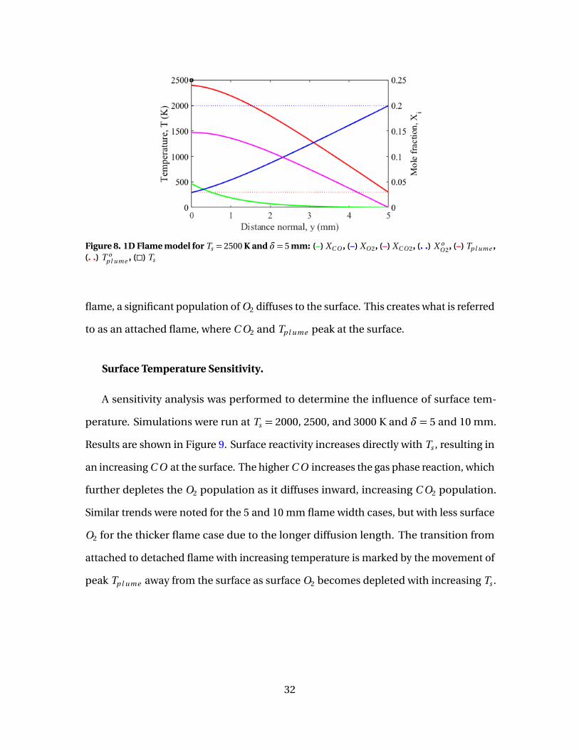
Figure 8. 1D Flame model for Ts = 2500 K andδ= 5 mm: (–) XC O , (–) XO 2, (–) XC O 2, (. .) X oO 2, (–) Tp l ume ,
(. .) T op l ume , (�) Ts
flame, a significant population of O2 diffuses to the surface. This creates what is referred
to as an attached flame, where C O2 and Tp l ume peak at the surface.
Surface Temperature Sensitivity.
A sensitivity analysis was performed to determine the influence of surface tem-
perature. Simulations were run at Ts = 2000, 2500, and 3000 K and δ = 5 and 10 mm.
Results are shown in Figure 9. Surface reactivity increases directly with Ts , resulting in
an increasing C O at the surface. The higher C O increases the gas phase reaction, which
further depletes the O2 population as it diffuses inward, increasing C O2 population.
Similar trends were noted for the 5 and 10 mm flame width cases, but with less surface
O2 for the thicker flame case due to the longer diffusion length. The transition from
attached to detached flame with increasing temperature is marked by the movement of
peak Tp l ume away from the surface as surface O2 becomes depleted with increasing Ts .
32
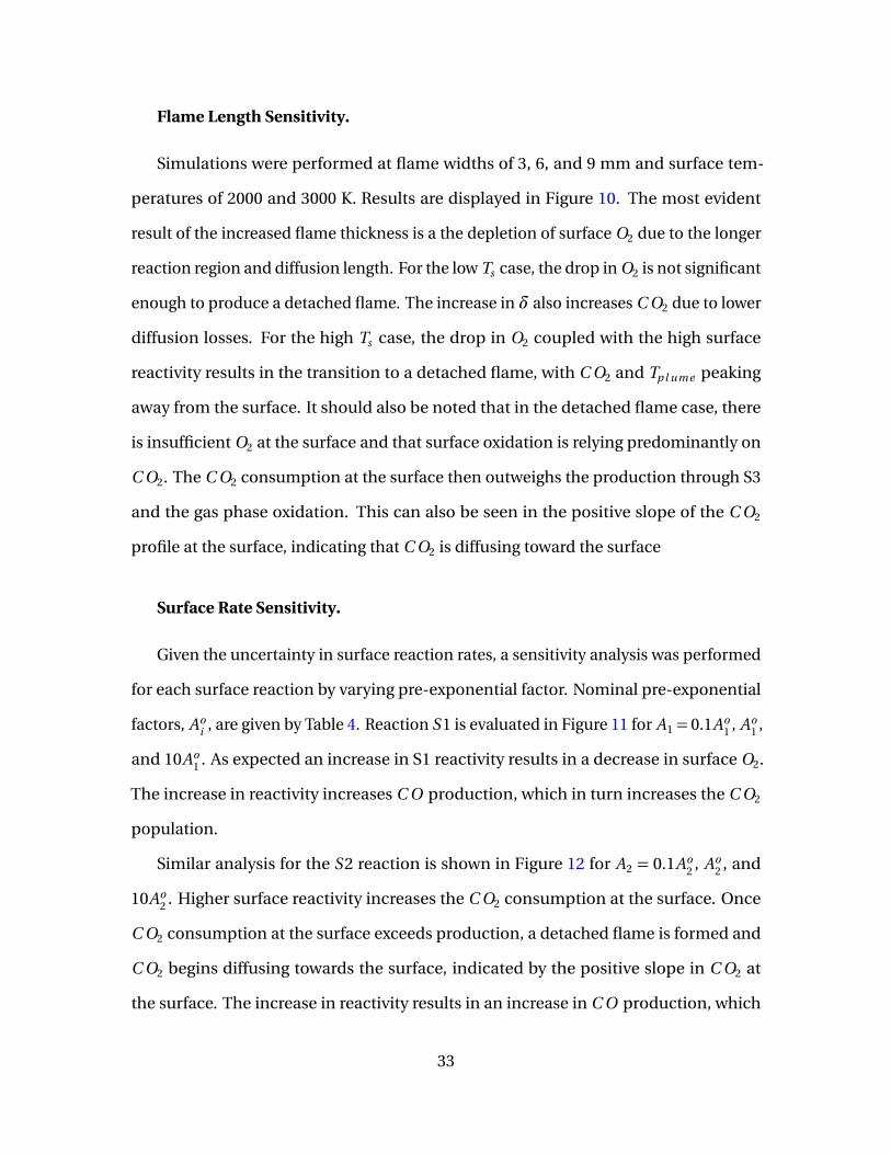
Flame Length Sensitivity.
Simulations were performed at flame widths of 3, 6, and 9 mm and surface tem-
peratures of 2000 and 3000 K. Results are displayed in Figure 10. The most evident
result of the increased flame thickness is a the depletion of surface O2 due to the longer
reaction region and diffusion length. For the low Ts case, the drop in O2 is not significant
enough to produce a detached flame. The increase in δ also increases C O2 due to lower
diffusion losses. For the high Ts case, the drop in O2 coupled with the high surface
reactivity results in the transition to a detached flame, with C O2 and Tp l ume peaking
away from the surface. It should also be noted that in the detached flame case, there
is insufficient O2 at the surface and that surface oxidation is relying predominantly on
C O2. The C O2 consumption at the surface then outweighs the production through S3
and the gas phase oxidation. This can also be seen in the positive slope of the C O2
profile at the surface, indicating that C O2 is diffusing toward the surface
Surface Rate Sensitivity.
Given the uncertainty in surface reaction rates, a sensitivity analysis was performed
for each surface reaction by varying pre-exponential factor. Nominal pre-exponential
factors, Aoi , are given by Table 4. Reaction S1 is evaluated in Figure 11 for A1 = 0.1Ao
1 , Ao1 ,
and 10Ao1 . As expected an increase in S1 reactivity results in a decrease in surface O2.
The increase in reactivity increases C O production, which in turn increases the C O2
population.
Similar analysis for the S2 reaction is shown in Figure 12 for A2 = 0.1Ao2 , Ao
2 , and
10Ao2 . Higher surface reactivity increases the C O2 consumption at the surface. Once
C O2 consumption at the surface exceeds production, a detached flame is formed and
C O2 begins diffusing towards the surface, indicated by the positive slope in C O2 at
the surface. The increase in reactivity results in an increase in C O production, which
33
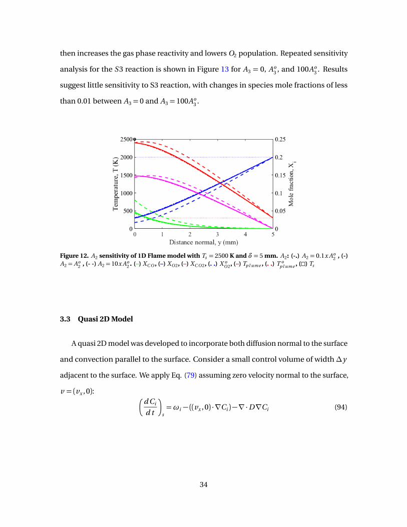
then increases the gas phase reactivity and lowers O2 population. Repeated sensitivity
analysis for the S3 reaction is shown in Figure 13 for A3 = 0, Ao3 , and 100Ao
3 . Results
suggest little sensitivity to S3 reaction, with changes in species mole fractions of less
than 0.01 between A3 = 0 and A3 = 100Ao3 .
Figure 12. A2 sensitivity of 1D Flame model with Ts = 2500 K and δ = 5 mm. A2: (-.) A2 = 0.1x Ao2 , (-)
A2 = Ao2 , (- -) A2 = 10x Ao
2 . (–) XC O , (–) XO 2, (–) XC O 2, (. .) X oO 2, (–) Tp l ume , (. .) T o
p l ume , (�) Ts
3.3 Quasi 2D Model
A quasi 2D model was developed to incorporate both diffusion normal to the surface
and convection parallel to the surface. Consider a small control volume of width∆y
adjacent to the surface. We apply Eq. (79) assuming zero velocity normal to the surface,
v = (vx , 0):�
d Ci
d t
�
s=ωi − ((vx , 0) ·∇Ci )−∇·D∇Ci (94)
34
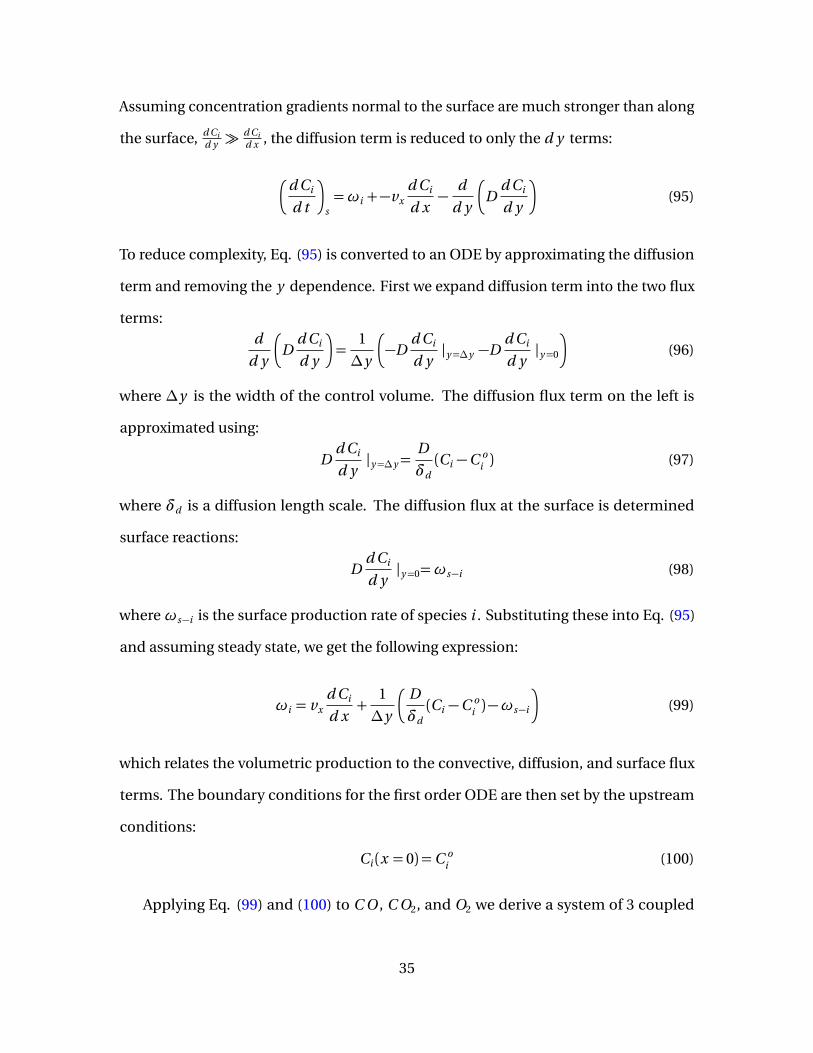
Assuming concentration gradients normal to the surface are much stronger than along
the surface, d Cid y �
d Cid x , the diffusion term is reduced to only the d y terms:
�
d Ci
d t
�
s=ωi +−vx
d Ci
d x−
d
d y
�
Dd Ci
d y
�
(95)
To reduce complexity, Eq. (95) is converted to an ODE by approximating the diffusion
term and removing the y dependence. First we expand diffusion term into the two flux
terms:d
d y
�
Dd Ci
d y
�
=1
∆y
�
−Dd Ci
d y|y=∆y −D
d Ci
d y|y=0
�
(96)
where ∆y is the width of the control volume. The diffusion flux term on the left is
approximated using:
Dd Ci
d y|y=∆y=
D
δd(Ci −C o
i ) (97)
where δd is a diffusion length scale. The diffusion flux at the surface is determined
surface reactions:
Dd Ci
d y|y=0=ωs−i (98)
whereωs−i is the surface production rate of species i . Substituting these into Eq. (95)
and assuming steady state, we get the following expression:
ωi = vx
d Ci
d x+
1
∆y
�
D
δd(Ci −C o
i )−ωs−i
�
(99)
which relates the volumetric production to the convective, diffusion, and surface flux
terms. The boundary conditions for the first order ODE are then set by the upstream
conditions:
Ci (x = 0) =C oi (100)
Applying Eq. (99) and (100) to C O , C O2, and O2 we derive a system of 3 coupled
35

ODEs and boundary conditions. Given surface and plume temperature profile inputs
to infer kinetic rates, the system can be solved numerically. A sensitivity analysis is
performed to determine the influence of Ts and flow rate. Key parameters used are
those given in Table 4.
Surface Temperature Sensitivity.
The simulation assumes a Gaussian Ts profile with width 10 cm and peaks of 2000,
2500, and 3000 K. The Gaussian plume temperature profile was fixed with a peak of
2200 K and half width 20 cm. Freestream velocity was fixed at 7 m/s. Diffusion length is
assumed be equal to boundary layer thickness, δd =δ(7 m/s). The resulting solutions
to the quasi 2D model with varying Ts are given in Figure 14. Surface reactivity increases
with surface temperature, resulting in an increase in C O due to S1 and S2. A dip in C O2
at laser center forms as the C O2 depletion through S2 overpowers gas phase production.
Flow Sensitivity.
Similar analysis was preformed for freestream flow conditions of 5, 7, and 10 m/s
to determine the role of convective transport. Temperature profiles were fixed with
peak Ts and Tp l ume of 3300 K and 2200 K, respectively, and half widths of 10 and 20 cm,
respectively. Diffusion length scale was assumed to scale with boundary layer thickness,
δd =δ∝ v −1/2∞ .
Simulation results are shown in Figure 15. The sensitivity to flow conditions can be
attributed to both diffusion and convection transport effects. The increase in freestream
flow conditions results in a decrease in boundary layer thickness, which decreases the
diffusion length scale. The C O population is then reduced due to higher diffusion losses.
Less C O2 is then produced due to the decrease in C O population. The convection
transport effects can be seen in the slight downstream shift of C O and C O2.
36
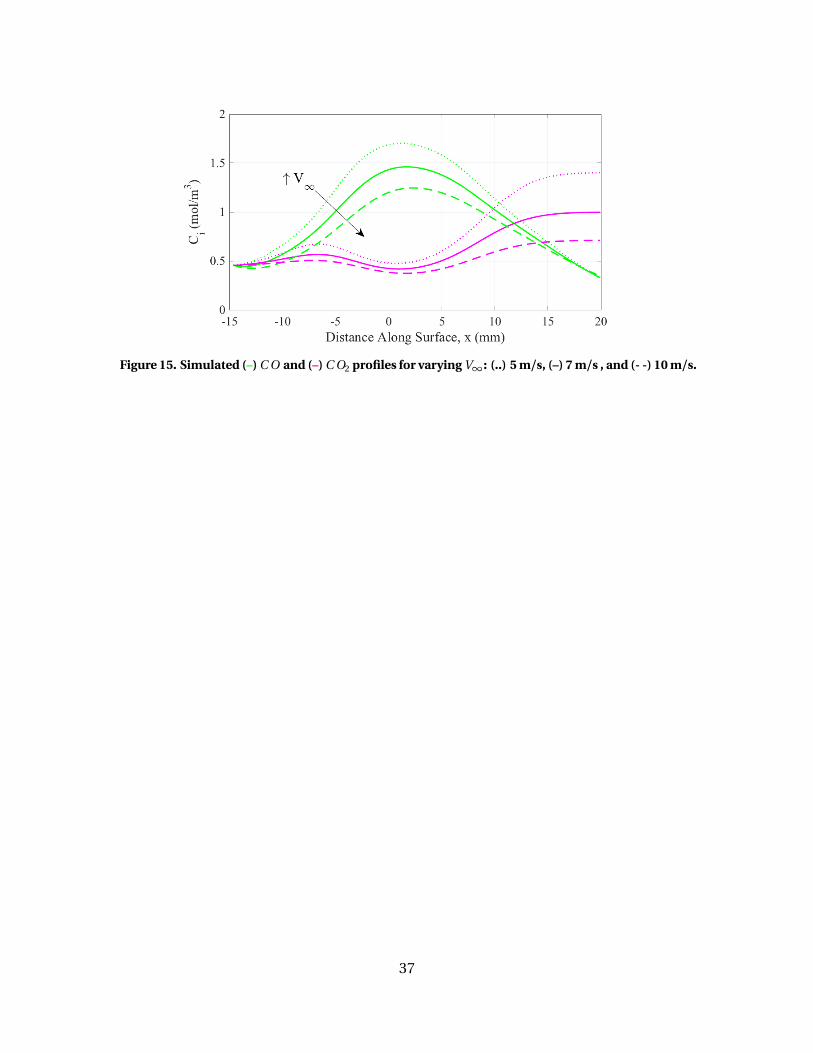
Figure 15. Simulated (–) C O and (–) C O2 profiles for varying V∞: (..) 5 m/s, (–) 7 m/s , and (- -) 10 m/s.
37
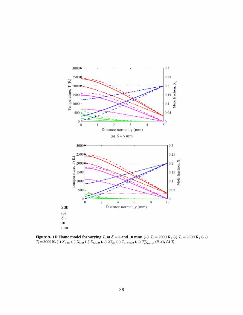
(a) δ= 5 mm
2(b)δ=10mm
00
Figure 9. 1D Flame model for varying Ts at δ = 5 and 10 mm: (-.) Ts = 2000 K , (-) Ts = 2500 K , (- -)Ts = 3000 K. (–) XC O , (–) XO 2, (–) XC O 2, (. .) X o
O 2, (–) Tp l ume , (. .) T op l ume , (F, �,�) Ts
38
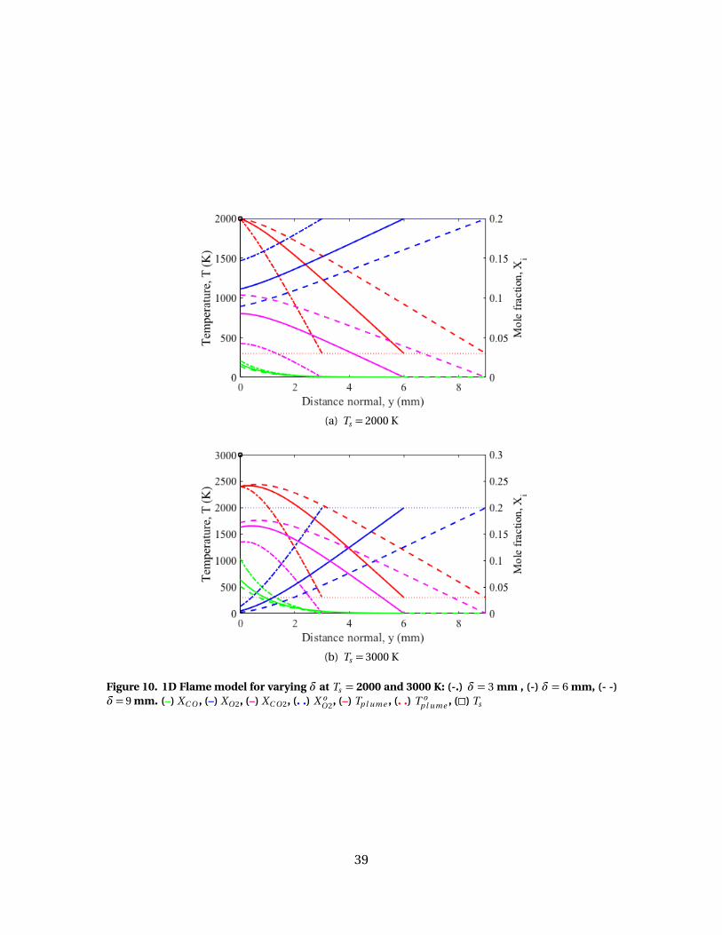
(a) Ts = 2000 K
(b) Ts = 3000 K
Figure 10. 1D Flame model for varying δ at Ts = 2000 and 3000 K: (-.) δ = 3 mm , (-) δ = 6 mm, (- -)δ= 9 mm. (–) XC O , (–) XO 2, (–) XC O 2, (. .) X o
O 2, (–) Tp l ume , (. .) T op l ume , (�) Ts
39
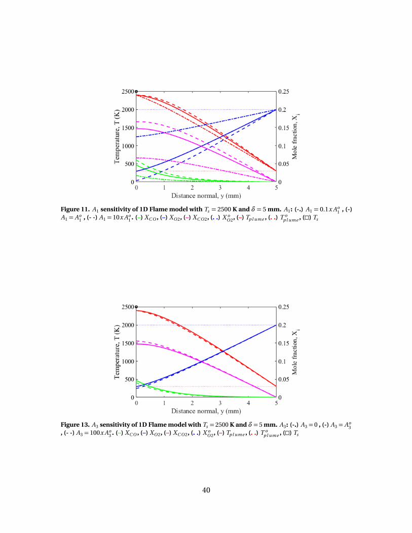
Figure 11. A1 sensitivity of 1D Flame model with Ts = 2500 K and δ = 5 mm. A1: (-.) A1 = 0.1x Ao1 , (-)
A1 = Ao1 , (- -) A1 = 10x Ao
1 . (–) XC O , (–) XO 2, (–) XC O 2, (. .) X oO 2, (–) Tp l ume , (. .) T o
p l ume , (�) Ts
Figure 13. A3 sensitivity of 1D Flame model with Ts = 2500 K and δ= 5 mm. A3: (-.) A3 = 0 , (-) A3 = Ao3
, (- -) A3 = 100x Ao3 . (–) XC O , (–) XO 2, (–) XC O 2, (. .) X o
O 2, (–) Tp l ume , (. .) T op l ume , (�) Ts
40
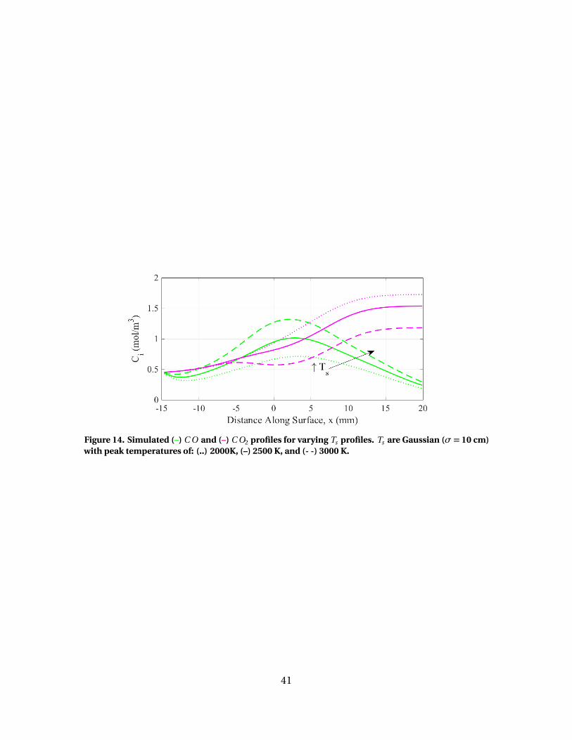
Figure 14. Simulated (–) C O and (–) C O2 profiles for varying Ts profiles. Ts are Gaussian (σ = 10 cm)with peak temperatures of: (..) 2000K, (–) 2500 K, and (- -) 3000 K.
41

IV. Experimental Methods
Chapter IV provides detail regarding the experimental procedures and post pro-
cessing techniques used in Chapter V - VII. Samples were tested at the Laser Hardened
Materials Laboratory (LHMEL) at Wright Patterson Air Force Base. A short summary of
the LHMEL laser system and beam diagnostics is given in Section 4.1. A description of
the three graphite materials is included in Section 4.2. A variety of MWIR and visible
diagnostics were used to monitor the gas and surface properties. Instrumentation
details, operating conditions, and post processing techniques are discussed in Section
4.3. Samples were tested at three flow configurations: buoyant flow, flat plate shear flow,
and stagnation flow. A description of each test configuration is given in Section 4.4.
4.1 Laser System and Diagnostics
Samples were irradiated using a 15 kW ytterbium fiber laser at 1.07 µm. Laser power
was characterized in two phases [55]. Prior to testing, a ballistic calorimeter was used
to measure the total power output. During testing, a small fraction of the beam is
routed to a transient calorimeter to measure power over the testing period. Spatial
characterization of the beam profile is completed using a small picked off portion of
the beam incident on a diffuse reflector and imaged using a high speed camera. The
irradiance is then determined based on calorimeter power measurements and the
imaged beam profile. Average irradiance over the beam profile is then determined by:
Ia v e = P /db (101)
where P is the total power, and db is the average beam diameter, defined as containing
86% of the beam power and determined using the beam profile images. A detailed
description of the LHMEL test facility and its capabilities can be found in [55–57].
42
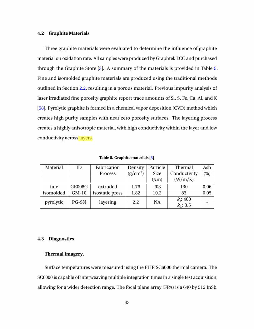
4.2 Graphite Materials
Three graphite materials were evaluated to determine the influence of graphite
material on oxidation rate. All samples were produced by Graphtek LCC and purchased
through the Graphite Store [3]. A summary of the materials is provided in Table 5.
Fine and isomolded graphite materials are produced using the traditional methods
outlined in Section 2.2, resulting in a porous material. Previous impurity analysis of
laser irradiated fine porosity graphite report trace amounts of Si, S, Fe, Ca, Al, and K
[58]. Pyrolytic graphite is formed in a chemical vapor deposition (CVD) method which
creates high purity samples with near zero porosity surfaces. The layering process
creates a highly anisotropic material, with high conductivity within the layer and low
conductivity across layers.
Table 5. Graphite materials [3]
Material ID Fabrication Density Particle Thermal AshProcess (g/cm3) Size Conductivity (%)
(µm) (W/m/K)
fine GR008G extruded 1.76 203 130 0.06isomolded GM-10 isostatic press 1.82 10.2 83 0.05
pyrolytic PG-SN layering 2.2 NAkq: 400
-k⊥: 3.5
4.3 Diagnostics
Thermal Imagery.
Surface temperatures were measured using the FLIR SC6000 thermal camera. The
SC6000 is capable of interweaving multiple integration times in a single test acquisition,
allowing for a wider detection range. The focal plane array (FPA) is a 640 by 512 InSb,
43
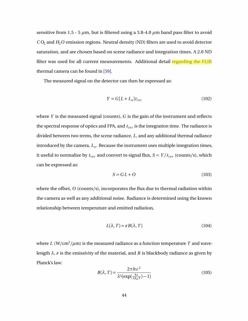
sensitive from 1.5 - 5 µm, but is filtered using a 3.8-4.0 µm band pass filter to avoid
C O2 and H2O emission regions. Neutral density (ND) filters are used to avoid detector
saturation, and are chosen based on scene radiance and integration times. A 2.0 ND
filter was used for all current measurements. Additional detail regarding the FLIR
thermal camera can be found in [59].
The measured signal on the detector can then be expressed as:
Y =G [L + Lo ]ti n t (102)
where Y is the measured signal (counts), G is the gain of the instrument and reflects
the spectral response of optics and FPA, and ti n t is the integration time. The radiance is
divided between two terms, the scene radiance, L , and any additional thermal radiance
introduced by the camera, Lo . Because the instrument uses multiple integration times,
it useful to normalize by ti n t and convert to signal flux, S = Y /ti n t (counts/s), which
can be expressed as:
S =G L +O (103)
where the offset, O (counts/s), incorporates the flux due to thermal radiation within
the camera as well as any additional noise. Radiance is determined using the known
relationship between temperature and emitted radiation,
L (λ, T ) = εB (λ, T ) (104)
where L (W/cm2/µm) is the measured radiance as a function temperature T and wave-
length λ, ε is the emissivity of the material, and B is blackbody radiance as given by
Planck’s law:
B (λ, T ) =2πh c 2
λ5(exp( h cλkB T )−1)
(105)
44

where kB is the Boltzmann constant, h is the Planck constant, and c is the speed of light.
The signal flux can then be expressed as:
S =G [εB (λF , T )] +O (106)
λF is the filtered FLIR wavelength, λF =3.9 µm.
G and O values are determined by measuring the signal flux of a wide area blackbody,
expressed as:
S =G [εB B B (λF , TB B )]+O (107)
where εB B is the emissivity of the blackbody, typically >0.96, and B (λF , TB B ) is the
blackbody radiance. Calibration is done in two phases. Prior to testing, blackbody
measurements are taken at surface temperatures of 300 - 870 K (blackbody limit) and
integration times of 0.01 - 2 ms to determine gain and offset. During testing, an addi-
tional calibration is done to determine any change in O , which is highly sensitive to
changes in ambient room temperature.
Post processing of thermal imagery consisted of three steps. First a non-linearity
correction is applied to account for the non-linear response at low signal. The signal
is then converted to a measured radiance using Eq. (103) and the determined gain
and offset. Lastly, surface temperature is computed using Eq. (104) and the inferred
radiance. In the case of multiple integration time data, this produces four tempera-
ture maps, each providing a limited temperature region based on the noise floor and
saturation limit. Shortest integration times were chosen to avoid saturation while still
capturing peak surface temperatures. The remaining integration times were increased
to capture a range of lower surface temperatures, ideally with the longest capturing
room temperature. The four temperature maps are then averaged together, neglecting
low signal or saturated pixels, to maximize detectable temperature range.
45
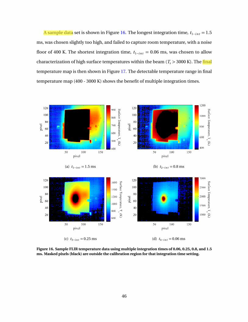
A sample data set is shown in Figure 16. The longest integration time, t1−i n t = 1.5
ms, was chosen slightly too high, and failed to capture room temperature, with a noise
floor of 400 K. The shortest integration time, t1−i n t = 0.06 ms, was chosen to allow
characterization of high surface temperatures within the beam (Ts > 3000 K). The final
temperature map is then shown in Figure 17. The detectable temperature range in final
temperature map (400 - 3000 K) shows the benefit of multiple integration times.
(a) t1−i n t = 1.5 ms (b) t2−i n t = 0.8 ms
(c) t3−i n t = 0.25 ms (d) t4−i n t = 0.06 ms
Figure 16. Sample FLIR temperature data using multiple integration times of 0.06, 0.25, 0.8, and 1.5ms. Masked pixels (black) are outside the calibration region for that integration time setting.
46
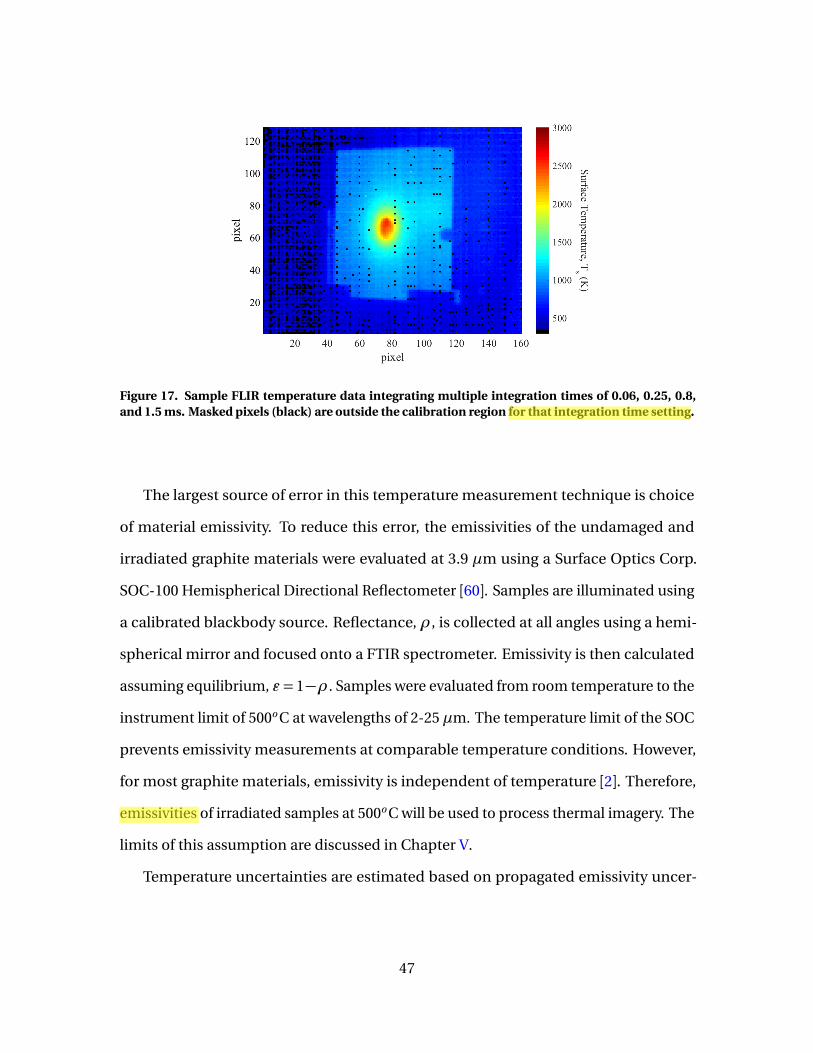
Figure 17. Sample FLIR temperature data integrating multiple integration times of 0.06, 0.25, 0.8,and 1.5 ms. Masked pixels (black) are outside the calibration region for that integration time setting.
The largest source of error in this temperature measurement technique is choice
of material emissivity. To reduce this error, the emissivities of the undamaged and
irradiated graphite materials were evaluated at 3.9 µm using a Surface Optics Corp.
SOC-100 Hemispherical Directional Reflectometer [60]. Samples are illuminated using
a calibrated blackbody source. Reflectance, ρ, is collected at all angles using a hemi-
spherical mirror and focused onto a FTIR spectrometer. Emissivity is then calculated
assuming equilibrium, ε = 1−ρ. Samples were evaluated from room temperature to the
instrument limit of 500o C at wavelengths of 2-25 µm. The temperature limit of the SOC
prevents emissivity measurements at comparable temperature conditions. However,
for most graphite materials, emissivity is independent of temperature [2]. Therefore,
emissivities of irradiated samples at 500o C will be used to process thermal imagery. The
limits of this assumption are discussed in Chapter V.
Temperature uncertainties are estimated based on propagated emissivity uncer-
47
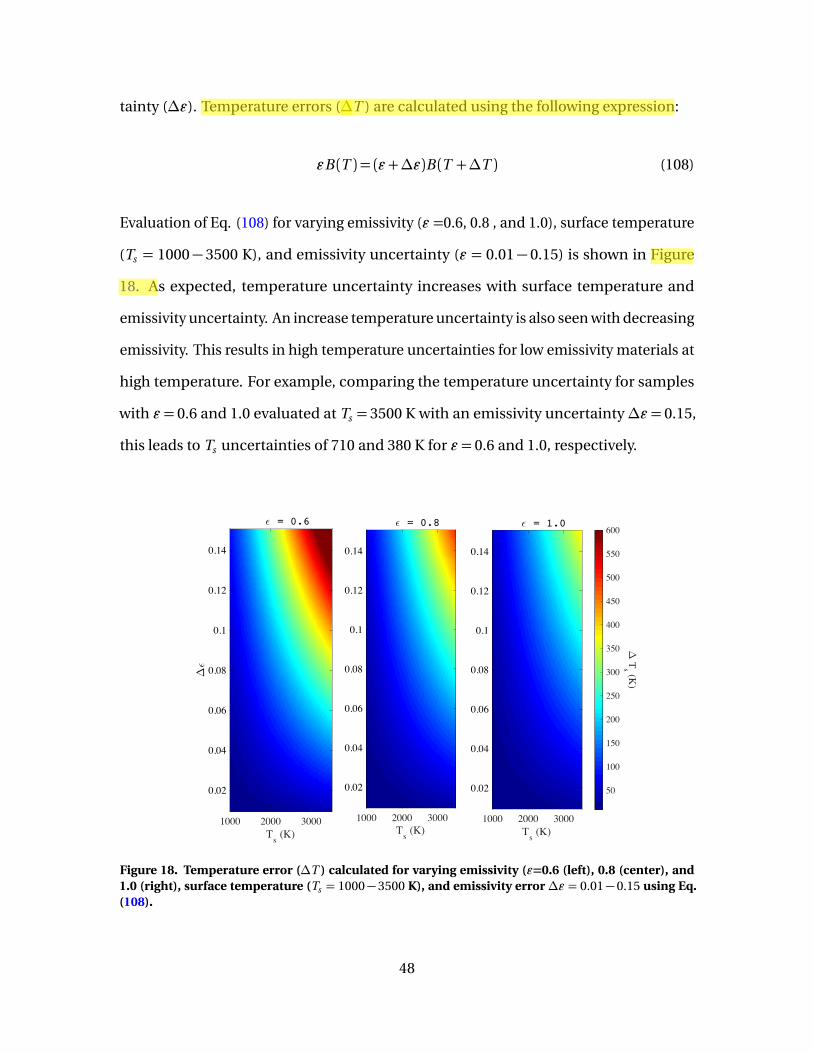
tainty (∆ε). Temperature errors (∆T ) are calculated using the following expression:
εB (T ) = (ε+∆ε)B (T +∆T ) (108)
Evaluation of Eq. (108) for varying emissivity (ε =0.6, 0.8 , and 1.0), surface temperature
(Ts = 1000− 3500 K), and emissivity uncertainty (ε = 0.01− 0.15) is shown in Figure
18. As expected, temperature uncertainty increases with surface temperature and
emissivity uncertainty. An increase temperature uncertainty is also seen with decreasing
emissivity. This results in high temperature uncertainties for low emissivity materials at
high temperature. For example, comparing the temperature uncertainty for samples
with ε = 0.6 and 1.0 evaluated at Ts = 3500 K with an emissivity uncertainty∆ε = 0.15,
this leads to Ts uncertainties of 710 and 380 K for ε = 0.6 and 1.0, respectively.
ϵ = 0.6
1000 2000 3000Ts (K)
0.02
0.04
0.06
0.08
0.1
0.12
0.14
∆ϵ
ϵ = 0.8
1000 2000 3000Ts (K)
0.02
0.04
0.06
0.08
0.1
0.12
0.14
ϵ = 1.0
1000 2000 3000Ts (K)
0.02
0.04
0.06
0.08
0.1
0.12
0.14
50
100
150
200
250
300
350
400
450
500
550
600
∆ T
s (K)
Figure 18. Temperature error (∆T ) calculated for varying emissivity (ε=0.6 (left), 0.8 (center), and1.0 (right), surface temperature (Ts = 1000− 3500 K), and emissivity error ∆ε = 0.01− 0.15 using Eq.(108).
48
Imaging Fourier Imaging Spectrometer.
The combustion plume was characterized using the Telops MWIR hyperspectral
imager. The MWIR Telops is an imaging Fourier Transform spectrometer (IFTS) which
provides spectral content at each pixel in a 320 by 256 InSb focal plane array (FPA).
The IFTS is responsive from 1800-6667 cm-1(λ= 1.5 - 5.5 µm) with a variable spectral
resolution of∆ν= 0.25 - 16 cm-1. Data rates vary with window size, with typical data
rates on the order of 1 Hz. Spatial resolution varies with standoff distance, with typical
values of 0.4-0.5 mm/pixel for the three flow configurations. Further detail regarding
the design and performance of the IFTS can be found in references [1, 7, 61, 62].
Instrument response is characterized using a two point calibration method [62].
Gain, G , and offset, O , are determined by measuring a wide area blackbody at two
temperatures. Blackbody temperatures are chosen to cover the dynamic range of the
instrument. The measured signals (Y1, Y2) can be expressed using Eq. (21):
Y1(ν) =G (ν) (B (ν, T1) +O (ν)) (109)
Y2(ν) =G (ν) (B (ν, T2) +O (ν)) (110)
where B (ν, Ti ) is the blackbody spectral radiance at temperature Ti . Gain and offset are
then calculated at each pixel in the FPA by solving Eq. (109) - (110) using measured Y1
and Y2 values.
Post processing of IFTS data was completed in three steps. First, data was temporally
averaged to improve signal to noise ratio. A fast Fourier transform is then used to
convert the measured interferogram to wavenumber space, Y (ν). Next, Eq. (21) is used
to convert Y (ν) to a calibrated radiance, L (ν). Sample IFTS data is shown in Figure
19. The broadband image on the left highlights limited calibration of the instrument.
Integration times are chosen to allow the high temperature plume to fall within the
49
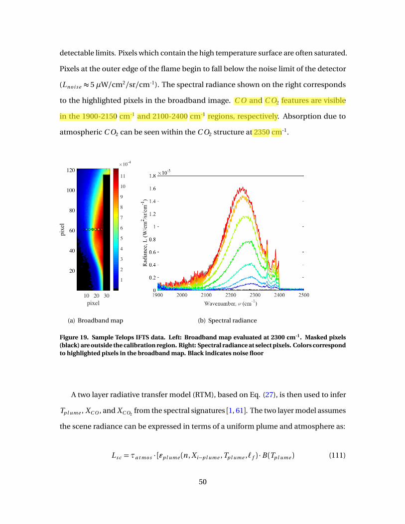
detectable limits. Pixels which contain the high temperature surface are often saturated.
Pixels at the outer edge of the flame begin to fall below the noise limit of the detector
(Lno i s e ≈ 5 µW/cm2/sr/cm-1). The spectral radiance shown on the right corresponds
to the highlighted pixels in the broadband image. C O and C O2 features are visible
in the 1900-2150 cm-1 and 2100-2400 cm-1 regions, respectively. Absorption due to
atmospheric C O2 can be seen within the C O2 structure at 2350 cm-1.
10 20 30pixel
20
40
60
80
100
120
pixel
1
2
3
4
5
6
7
8
9
10
11
×10-4
(a) Broadband map (b) Spectral radiance
Figure 19. Sample Telops IFTS data. Left: Broadband map evaluated at 2300 cm-1. Masked pixels(black) are outside the calibration region. Right: Spectral radiance at select pixels. Colors correspondto highlighted pixels in the broadband map. Black indicates noise floor
A two layer radiative transfer model (RTM), based on Eq. (27), is then used to infer
Tp l ume , XC O , and XC O2from the spectral signatures [1, 61]. The two layer model assumes
the scene radiance can be expressed in terms of a uniform plume and atmosphere as:
L s c =τa t mo s · [εp l ume (n , X i−p l ume , Tp l ume ,` f ) ·B (Tp l ume ) (111)
50
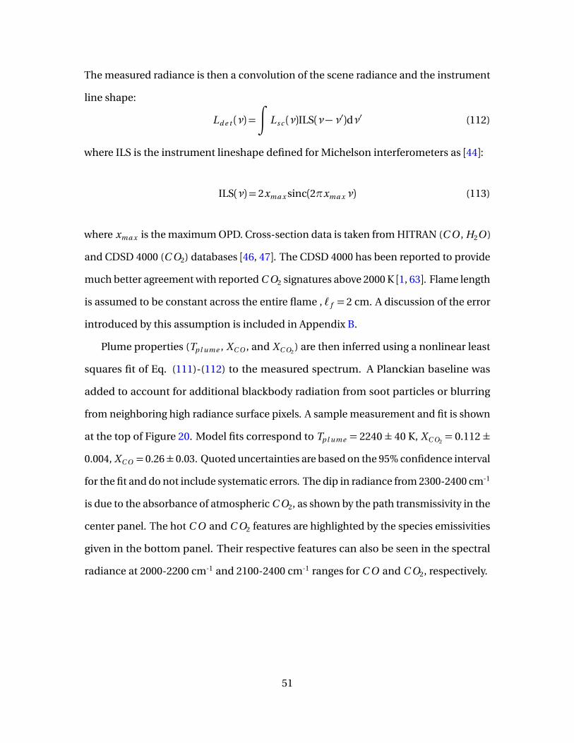
The measured radiance is then a convolution of the scene radiance and the instrument
line shape:
Ld e t (ν) =
∫
L s c (ν)ILS(ν−ν′)dν′ (112)
where ILS is the instrument lineshape defined for Michelson interferometers as [44]:
ILS(ν) = 2xma x sinc(2πxma xν) (113)
where xma x is the maximum OPD. Cross-section data is taken from HITRAN (C O , H2O )
and CDSD 4000 (C O2) databases [46, 47]. The CDSD 4000 has been reported to provide
much better agreement with reported C O2 signatures above 2000 K [1, 63]. Flame length
is assumed to be constant across the entire flame , ` f = 2 cm. A discussion of the error
introduced by this assumption is included in Appendix B.
Plume properties (Tp l ume , XC O , and XC O2) are then inferred using a nonlinear least
squares fit of Eq. (111)-(112) to the measured spectrum. A Planckian baseline was
added to account for additional blackbody radiation from soot particles or blurring
from neighboring high radiance surface pixels. A sample measurement and fit is shown
at the top of Figure 20. Model fits correspond to Tp l ume = 2240 ± 40 K, XC O2= 0.112 ±
0.004, XC O = 0.26± 0.03. Quoted uncertainties are based on the 95% confidence interval
for the fit and do not include systematic errors. The dip in radiance from 2300-2400 cm-1
is due to the absorbance of atmospheric C O2, as shown by the path transmissivity in the
center panel. The hot C O and C O2 features are highlighted by the species emissivities
given in the bottom panel. Their respective features can also be seen in the spectral
radiance at 2000-2200 cm-1 and 2100-2400 cm-1 ranges for C O and C O2, respectively.
51

Figure 20. Sample measured spectra and model. (-·-) measured radiance, Ld e t ; (–) modeled radiance;(–) path transmission,τa t mo s ; (–) C O emissivity, εC O ; (–) C O2 emissivity, εC O 2. Model fits correspondto Tp l ume = 2240 ± 40 K, XC O2
= 0.112 ± 0.004, XC O = 0.26 ± 0.03
Full 2D spatial maps of species concentration and plume temperature are then
inferred by fitting spectra at each pixel. Sample species and temperature maps as well
as uncertainty maps are given in Figure 21. Masked values (black) represent pixels
without fits due to inadequate signal. Uncertainties are based on the 95% confidence
bounds of the fit and do not include systematic error. In general, plume temperature
errors < 2% for Tp l ume = 1800−2500 K and species mole fraction uncertainties of < 10%
52
for X i > 0.1 are observed. Some fit issues arise in areas of the plume with little C O ,
leading to higher uncertainties in temperature fits, as seen by the higher temperature
uncertainties at flame edge.
Two possible additional sources of error are line of sight averaging and pixel blurring.
Error estimates for line of sight averaging are provided in Appendix B. Results suggest
systematic errors of < 12% for species mole fraction and < 10% for plume temperature.
To quantify the severity of the blurring, measurements of the edge spread function (ESF)
were taken using a knife edge and blackbody. At focus, pixel blurring is minimal with
less than 5% of radiant energy being deposited in neighboring pixels. The most severe
blurring is expected at the sample surface, where the hot sample edge is 3.8 cm off focus,
causing a 10 % deposit of signature into the neighboring pixels. In some cases this may
result in falsely identifying the sample surface. Further detail regarding the MW Telops
and its use a combustion diagnostic can be found in [7, 61, 62, 64].
53
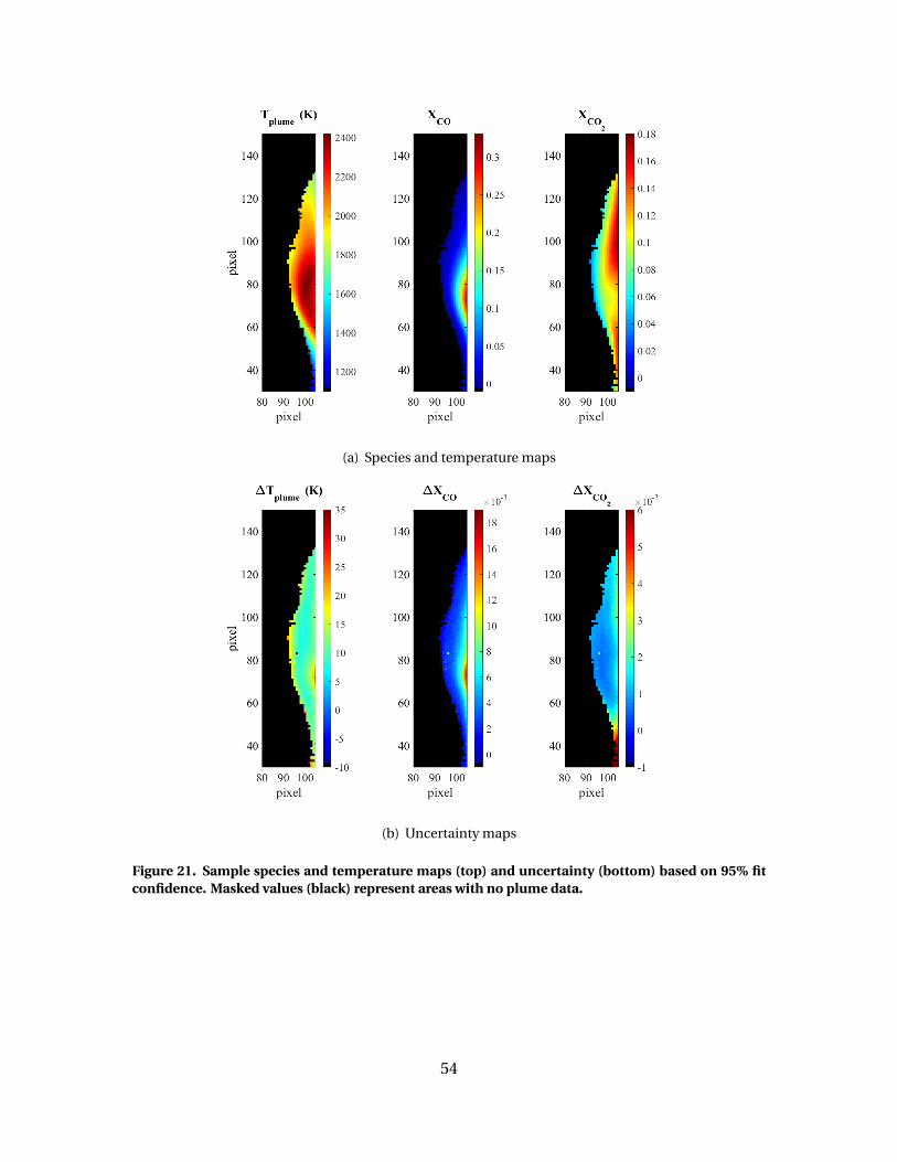
(a) Species and temperature maps
(b) Uncertainty maps
Figure 21. Sample species and temperature maps (top) and uncertainty (bottom) based on 95% fitconfidence. Masked values (black) represent areas with no plume data.
54
Visible Imagery.
Several visible cameras were used to monitor the test facility and sample during
testing. LHMEL witness cameras were time synchronized with laser control system,
allowing for accurate determination of time to ignition. High speed imagery (300
frames/s) of the combustion plume was taken using the Phantom v7 visible high speed
camera. High speed imagery was used to visualize flow patterns and estimate the flow
velocity through particulate tracking.
4.4 Flow Variations
Measurements were taken under three flow conditions: buoyant flow, flat plate
shear flow, and stagnation flow. A description of each of test configuration is discussed
below.
Buoyant Flow.
In the buoyant configuration, samples were irradiated in an open air environment,
creating a buoyant flame. Three graphite materials (fine, isomolded, and pyrolytic)
were evaluated at two irradiances (1000, 3600 W/cm2) for 180 s to produce steady state
temperatures of up to 3100 K. Buoyant flow configuration is shown in Figure 22. Samples
were mounted perpendicular to the beam in an open air environment (20% O2, < 1%
H2O ). Surface temperatures are observed using the MWIR thermal imager mounted 51
degrees from normal. The resulting buoyant flame is observed along the z axis using the
MW IFTS and visible high speed camera. Species and temperature maps are produced
from temporally averaged steady state IFTS data, from 100 - 150 s, to improve SNR.
55

Flat Plate Shear Flow.
In the flat plate shear flow configuration, samples were irradiated while in a flat
plate shear flow, as shown in Figure 23. Three graphite materials (fine, isomolded, and
pyrolytic) were evaluated three flow speeds (5, 7, and 10 m/s) and two irradiances (750,
1500 W/cm2) for 120 s to produce steady state temperatures of up to 3000 K. Samples
were mounted in a small wind tunnel, flush with the test section floor, 15 cm downstream
of the established flow. The test section was equipped with side and top optical access
to allow for thermal imagery of the surface and side imaging of the plume. Dry air (20%
O2, < 1% H2O ) was used to establish flows of 5, 7, and 10 m/s. Reynolds number for
the 10 m/s case is well below turbulent thresholds (Ret u r b ≈ 105), for both for reacting
and non-reacting flow estimates: non-reacting: Re (300 K, 10 m/s) = 7 ·104, reacting:
Re (2000 K, 10 m/s)= 3 · 103. Expansion to higher speed laminar flow was limited by
boundary layer thickness and the spatial resolution of the IFTS (0.5 mm/pixel). Species
and temperature maps are produced from temporally averaged steady state IFTS data,
from 80 - 100 s, to improve SNR.
Stagnation Flow.
The stagnation flow configuration is depicted in Figure 24. Stagnation flow was
established using a 2.5 cm diameter nozzle, designed to produce a flat top exit flow. A 1.5
m/s dry air (< 2% H2O ) flow was established over the 6 in diameter cone test samples,
creating a 3D stagnation flow with stagnation velocity gradient, B = 3v∞/d = 30 s-1
(v∞ - flow velocity, d - sample diameter). Fine porosity samples were irradiated at 660
and 900 W /c m 2 until reaching surface temperatures of up to 2500 K. IFTS data was
temporally averaged over 10 s windows to improve SNR. The resulting evolving plume
data is then compared with surface temperature measurements.
56
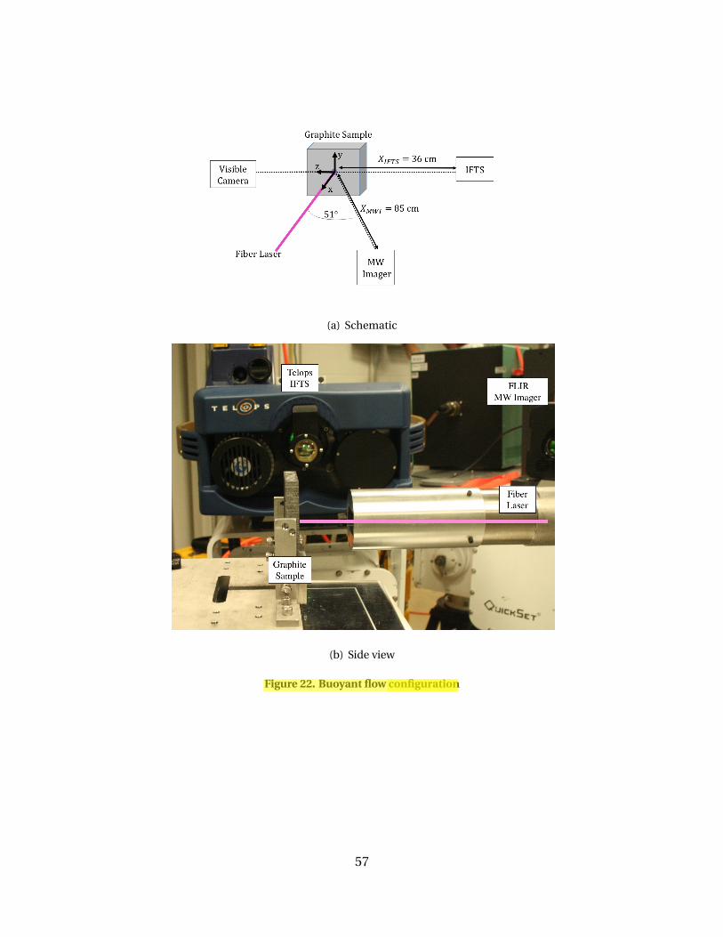
(a) Schematic
(b) Side view
Figure 22. Buoyant flow configuration
57
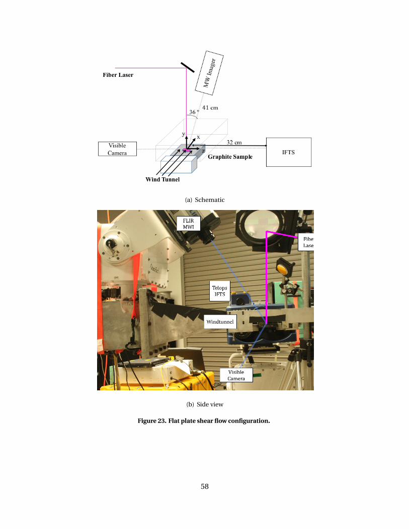
(a) Schematic
(b) Side view
Figure 23. Flat plate shear flow configuration.
58
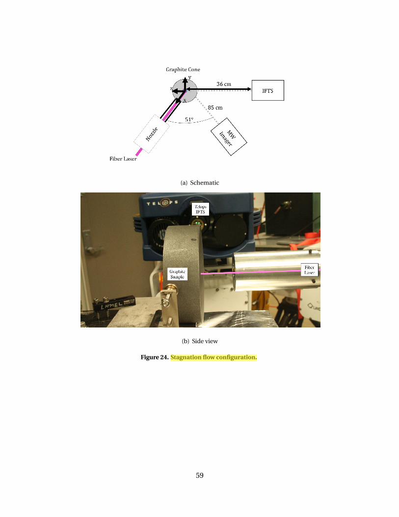
(a) Schematic
(b) Side view
Figure 24. Stagnation flow configuration.
59

V. Imaging Fourier Transform Spectroscopy of Graphite Oxidation ina Buoyant Flow
This chapter focuses on detailing the use the IFTS to characterize graphite oxidation
in buoyant flow, in partial fulfillment of objective 1. The application of oxidation models,
developed in Chapter III, are also discussed, in partial fulfillment of objective 2. The
chapter is written in journal article format and can be read independently as a stand
alone document. Additional details regarding background and experimental method
can be found in Chapter II and IV, respectively.
5.1 Abstract
The oxidation of laser irradiated graphite is investigated for varying porosity and sur-
face temperatures of 1500 - 3100 K at atmospheric pressure. Samples are irradiated using
a 1.07µm fiber laser at irradiances of 1000 and 3600 W/cm2 in dry air environment (20%
O2,< 1% H2O ), producing a buoyant flow. Combustion plumes are analyzed using a mid-
wave (MW) imaging Fourier transform spectrometer (IFTS) at 2 cm-1 spectral resolution,
0.5 mm/pixel spatial resolution, and data cube rates of 1 Hz. Spectral signatures feature
emission from C O and C O2 in the 1800 - 2500 cm-1 spectral region. A radiative transfer
model and cross-section data is used to infer species concentration and temperature
from hyperspectral data, resulting in 2D characterization of the reacting boundary layer.
Plume temperatures of up to 2500 K are observed. C O and C O2 populations are highly
correlated with temperature, with a general trend of [C O ]/[C O2] = 22exp(−6,000/Ts ).
A simplified model incorporating diffusion transport and surface kinetics is presented
to assess the relative strengths of the S1) 2C +O2 ⇒ 2C O , S2) C +C O2 ⇒ 2C O , and
S3) C +O2 ⇒ C O2 surface oxidation mechanisms. The role of kinetic and transport
mechanisms is discussed.
60
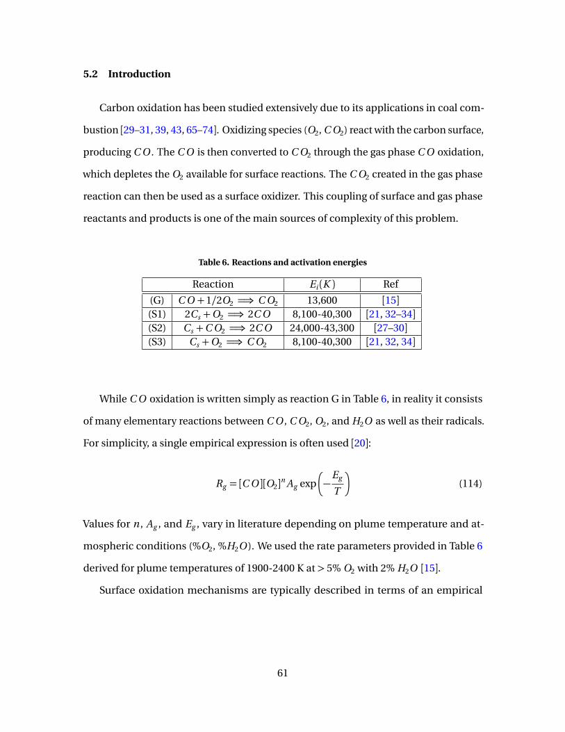
5.2 Introduction
Carbon oxidation has been studied extensively due to its applications in coal com-
bustion [29–31, 39, 43, 65–74]. Oxidizing species (O2, C O2) react with the carbon surface,
producing C O . The C O is then converted to C O2 through the gas phase C O oxidation,
which depletes the O2 available for surface reactions. The C O2 created in the gas phase
reaction can then be used as a surface oxidizer. This coupling of surface and gas phase
reactants and products is one of the main sources of complexity of this problem.
Table 6. Reactions and activation energies
Reaction Ei (K ) Ref
(G) C O +1/2O2 =⇒ C O2 13,600 [15](S1) 2Cs +O2 =⇒ 2C O 8,100-40,300 [21, 32–34](S2) Cs +C O2 =⇒ 2C O 24,000-43,300 [27–30](S3) Cs +O2 =⇒ C O2 8,100-40,300 [21, 32, 34]
While C O oxidation is written simply as reaction G in Table 6, in reality it consists
of many elementary reactions between C O , C O2, O2, and H2O as well as their radicals.
For simplicity, a single empirical expression is often used [20]:
Rg = [C O ][O2]n Ag exp
�
−Eg
T
�
(114)
Values for n , Ag , and Eg , vary in literature depending on plume temperature and at-
mospheric conditions (%O2, %H2O ). We used the rate parameters provided in Table 6
derived for plume temperatures of 1900-2400 K at > 5% O2 with 2% H2O [15].
Surface oxidation mechanisms are typically described in terms of an empirical
61
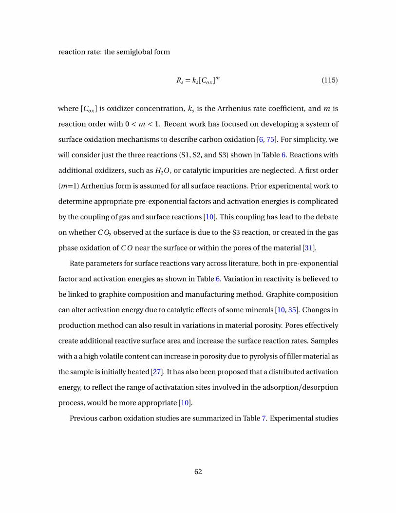
reaction rate: the semiglobal form
Rs = ks [Co x ]m (115)
where [Co x ] is oxidizer concentration, ks is the Arrhenius rate coefficient, and m is
reaction order with 0 < m < 1. Recent work has focused on developing a system of
surface oxidation mechanisms to describe carbon oxidation [6, 75]. For simplicity, we
will consider just the three reactions (S1, S2, and S3) shown in Table 6. Reactions with
additional oxidizers, such as H2O , or catalytic impurities are neglected. A first order
(m=1) Arrhenius form is assumed for all surface reactions. Prior experimental work to
determine appropriate pre-exponential factors and activation energies is complicated
by the coupling of gas and surface reactions [10]. This coupling has lead to the debate
on whether C O2 observed at the surface is due to the S3 reaction, or created in the gas
phase oxidation of C O near the surface or within the pores of the material [31].
Rate parameters for surface reactions vary across literature, both in pre-exponential
factor and activation energies as shown in Table 6. Variation in reactivity is believed to
be linked to graphite composition and manufacturing method. Graphite composition
can alter activation energy due to catalytic effects of some minerals [10, 35]. Changes in
production method can also result in variations in material porosity. Pores effectively
create additional reactive surface area and increase the surface reaction rates. Samples
with a a high volatile content can increase in porosity due to pyrolysis of filler material as
the sample is initially heated [27]. It has also been proposed that a distributed activation
energy, to reflect the range of activatation sites involved in the adsorption/desorption
process, would be more appropriate [10].
Previous carbon oxidation studies are summarized in Table 7. Experimental studies
62
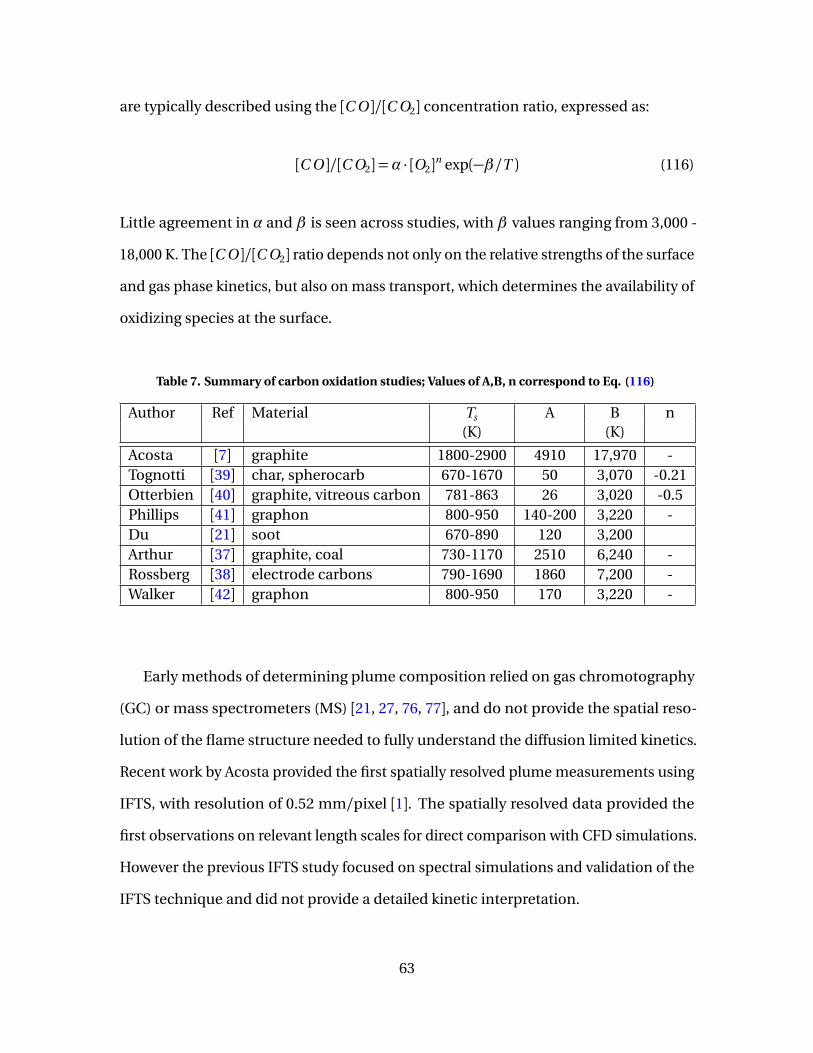
are typically described using the [C O ]/[C O2] concentration ratio, expressed as:
[C O ]/[C O2] =α · [O2]n exp(−β/T ) (116)
Little agreement in α and β is seen across studies, with β values ranging from 3,000 -
18,000 K. The [C O ]/[C O2] ratio depends not only on the relative strengths of the surface
and gas phase kinetics, but also on mass transport, which determines the availability of
oxidizing species at the surface.
Table 7. Summary of carbon oxidation studies; Values of A,B, n correspond to Eq. (116)
Author Ref Material Ts A B n(K) (K)
Acosta [7] graphite 1800-2900 4910 17,970 -Tognotti [39] char, spherocarb 670-1670 50 3,070 -0.21Otterbien [40] graphite, vitreous carbon 781-863 26 3,020 -0.5Phillips [41] graphon 800-950 140-200 3,220 -Du [21] soot 670-890 120 3,200Arthur [37] graphite, coal 730-1170 2510 6,240 -Rossberg [38] electrode carbons 790-1690 1860 7,200 -Walker [42] graphon 800-950 170 3,220 -
Early methods of determining plume composition relied on gas chromotography
(GC) or mass spectrometers (MS) [21, 27, 76, 77], and do not provide the spatial reso-
lution of the flame structure needed to fully understand the diffusion limited kinetics.
Recent work by Acosta provided the first spatially resolved plume measurements using
IFTS, with resolution of 0.52 mm/pixel [1]. The spatially resolved data provided the
first observations on relevant length scales for direct comparison with CFD simulations.
However the previous IFTS study focused on spectral simulations and validation of the
IFTS technique and did not provide a detailed kinetic interpretation.
63
The current study focuses on characterizing the oxidation of carbon surface as a
function of temperature and graphite material. Measurements presented utilize the
IFTS plume characterization technique developed by Acosta, with the addition of ther-
mal imaging to provide spatially resolved surface temperatures. The current study
expands the range of oxidation conditions, avoids significant particulate ejection and
minimizes surface erosion. Three graphite samples are evaluated at surface tempera-
tures of 1500-3100 K to determine dependence on material and surface temperature.
Species and temperature maps are inferred from hyperspectral imagery. Diffusion
transport is estimated using species gradients provided by the 2D species maps. A quasi
2D model incorporating diffusion and kinetics is also presented.
5.3 Experimental
Three graphite materials were each irradiated at 1000 and 3600 W/cm2 for 180 s
to produce steady state surface temperatures of 1500 - 3100 K. Samples were tested at
the Wright-Patterson Air Force Base Laser Hardened Materials Evaluation Laboratory
(LHMEL) using a 15 kW fiber laser at 1.07 µm, which produced a 1.4±0.2 cm diameter
(defined as 1/e 2) Gaussian beam. Quoted irradiance values of 1000 and 3600 W/cm2 are
spatially averaged over the beam profile. High and low irradiance conditions were cho-
sen to observe a wide range of surface temperature conditions, but avoid sublimation
(Ts > 3900 K).
A schematic of the experimental set-up is shown in Figure 25. Samples were mounted
perpendicular to the beam in an open air environment (20% O2, < 1% H2O ). The
resulting buoyant flame is observed along the z axis using the MW IFTS and Phantom
v7 visible high speed camera. Hyperspectral imagery is used to characterize plume
properties (C O , C O2, Tp ). Surface temperatures are observed using a FLIR SC6000
MWIR thermal imager mounted 51 degrees from normal.
64
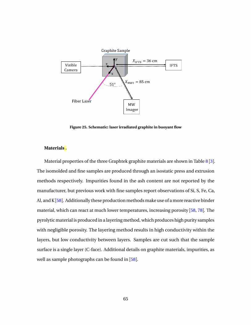
Figure 25. Schematic: laser irradiated graphite in buoyant flow
Materials .
Material properties of the three Graphtek graphite materials are shown in Table 8 [3].
The isomolded and fine samples are produced through an isostatic press and extrusion
methods respectively. Impurities found in the ash content are not reported by the
manufacturer, but previous work with fine samples report observations of Si, S, Fe, Ca,
Al, and K [58]. Additionally these production methods make use of a more reactive binder
material, which can react at much lower temperatures, increasing porosity [58, 78]. The
pyrolytic material is produced in a layering method, which produces high purity samples
with negligible porosity. The layering method results in high conductivity within the
layers, but low conductivity between layers. Samples are cut such that the sample
surface is a single layer (C-face). Additional details on graphite materials, impurities, as
well as sample photographs can be found in [58].
65
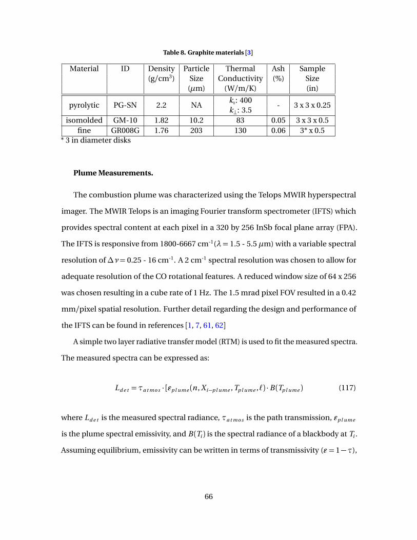
Table 8. Graphite materials [3]
Material ID Density Particle Thermal Ash Sample(g/cm3) Size Conductivity (%) Size
(µm) (W/m/K) (in)
pyrolytic PG-SN 2.2 NAkq: 400
- 3 x 3 x 0.25k⊥: 3.5
isomolded GM-10 1.82 10.2 83 0.05 3 x 3 x 0.5fine GR008G 1.76 203 130 0.06 3* x 0.5
* 3 in diameter disks
Plume Measurements.
The combustion plume was characterized using the Telops MWIR hyperspectral
imager. The MWIR Telops is an imaging Fourier transform spectrometer (IFTS) which
provides spectral content at each pixel in a 320 by 256 InSb focal plane array (FPA).
The IFTS is responsive from 1800-6667 cm-1(λ= 1.5 - 5.5 µm) with a variable spectral
resolution of∆ν= 0.25 - 16 cm-1. A 2 cm-1 spectral resolution was chosen to allow for
adequate resolution of the CO rotational features. A reduced window size of 64 x 256
was chosen resulting in a cube rate of 1 Hz. The 1.5 mrad pixel FOV resulted in a 0.42
mm/pixel spatial resolution. Further detail regarding the design and performance of
the IFTS can be found in references [1, 7, 61, 62]
A simple two layer radiative transfer model (RTM) is used to fit the measured spectra.
The measured spectra can be expressed as:
Ld e t =τa t mo s · [εp l ume (n , X i−p l ume , Tp l ume ,`) ·B (Tp l ume ) (117)
where Ld e t is the measured spectral radiance, τa t mo s is the path transmission, εp l ume
is the plume spectral emissivity, and B (Ti ) is the spectral radiance of a blackbody at Ti .
Assuming equilibrium, emissivity can be written in terms of transmissivity (ε = 1−τ),
66
with transmissivity defined by Beer’s law:
τ= exp(−nl∑
k
Xkσk (ν, Tp l ume )) (118)
where n is the number density, l is the path length, Xk is the plume species mole fraction,
and σk is the species cross-section taken from HITRAN (C O , H2O ) and CDSD 4000
(C O2) databases [46, 47]. The recent addition of the CDSD 4000 high temperature C O2
cross-sections has been reported to provide much better agreement with reported C O2
signatures above 2000 K [1, 63]. A least squares fitting routine with Equation 117 is
used to infer Tp l ume , XC O , and XC O2from the spectral signatures [1, 61]. A Planckian
baseline was added to account for broadband emission observed in pixels near the
sample surface, typically less than 10 µW/cm2/sr/cm-1, which is attributed to slight
blurring from radiating sample surface. Full 2D spatial maps of species concentration
and plume temperature are inferred by fitting spectra at each pixel.
Uncertainties quoted for plume properties are based on the 95% confidence bounds
of the fit and do not include systematic error. Plume temperature errors of less than
2% are observed for Tp l ume = 1800−2500 K. C O2 uncertainties were typically 2−10%,
with higher uncertainty for the low signal cases. Uncertainties for C O decrease with
increasing concentrations, with uncertainties of < 20% for XC O > 0.01 and < 10% for
XC O > 0.1. Two possible additional sources of error are line of sight averaging and pixel
blurring. Error estimates for line of sight averaging are provided in Appendix B. Results
suggest systematic errors of < 12% for species mole fraction and < 10% for plume
temperature. To quantify the severity of the blurring, measurements of the edge spread
function (ESF) were taken using a knife edge and blackbody. At focus, pixel blurring
is minimal with less than 5% of radiant energy being deposited in neighboring pixels.
However the most severe blurring is expected at the sample surface, where the hot
sample edge is 3.8 cm off focus, causing a 10 % deposit of signature into the neighboring
67
pixels. In some cases this may result in falsely identifying the sample surface. Further
detail regarding the MW Telops and its use a combustion diagnostic can be found in
[1, 61, 64, 79–81].
Thermal Measurements.
Surface temperatures were measured using the FLIR SC6000 thermal camera equipped
with a 620 by 512 FPA sensitive at 3.8-4.0 µm. The SC6000 is capable of interweaving
multiple integration times in a single test acquisition, allowing for a wider detection
range. Thermal measurements were taken using a 2.0 ND filter and integration times
of 0.1-1.5 ms, resulting in a noise floor of 600 K. Images were taken at 10 Hz and win-
dow size of 128x160 to reduce data volume. The FLIR was mounted 51° off normal to
avoid laser path, resulting in vertical and horizontal spatial resolutions of 0.8 and 1.2
mm/pixel respectively.
Camera signal is converted to temperature measurements using an external black-
body (320-870 K) and calibration scheme [82]. The largest source of error in this method
is the choice of material emissivity. Emissivities can vary across graphite materials,
with most isotropic graphite materials showing high emissivity (ε > 0.8), while pyrolytic
graphite exhibiting emissivities as low at 0.4 [2, 83, 84]. Additionally, surface roughness
can increase emissivity. In the laser damage scenario, this would result in an increase
in emissivity from the low undamaged emissivity to a surface roughness dependent
emissivity as the sample is irradiated. To improve surface temperature measurements,
the emissivities of the graphite materials used in this study were evaluated using a
Surface Optics Corp. SOC-100 Hemispherical Directional Reflectometer. Samples are
illuminated using a calibrated blackbody source. Reflectance, ρ, is collected at all an-
gles using a hemispherical mirror and focused onto a FTIR spectrometer. Emissivity
is then calculated assuming equilibrium, ε = 1−ρ. Further details regarding the SOC
68
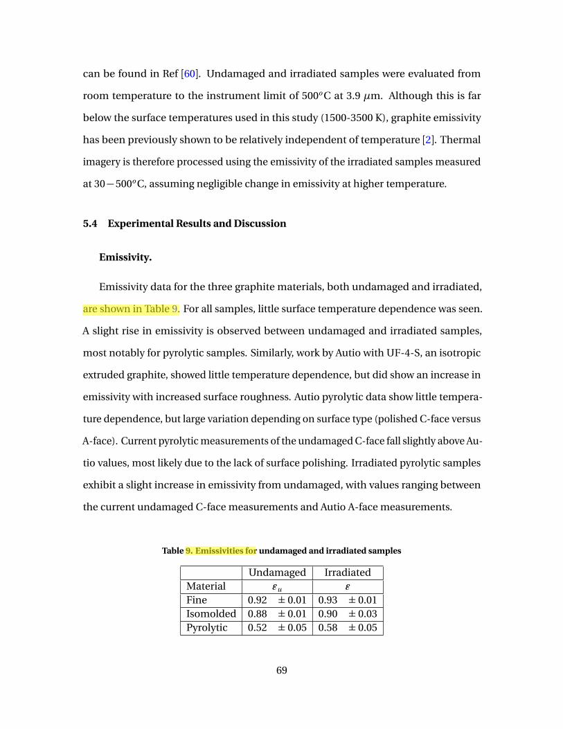
can be found in Ref [60]. Undamaged and irradiated samples were evaluated from
room temperature to the instrument limit of 500o C at 3.9 µm. Although this is far
below the surface temperatures used in this study (1500-3500 K), graphite emissivity
has been previously shown to be relatively independent of temperature [2]. Thermal
imagery is therefore processed using the emissivity of the irradiated samples measured
at 30−500o C, assuming negligible change in emissivity at higher temperature.
5.4 Experimental Results and Discussion
Emissivity.
Emissivity data for the three graphite materials, both undamaged and irradiated,
are shown in Table 9. For all samples, little surface temperature dependence was seen.
A slight rise in emissivity is observed between undamaged and irradiated samples,
most notably for pyrolytic samples. Similarly, work by Autio with UF-4-S, an isotropic
extruded graphite, showed little temperature dependence, but did show an increase in
emissivity with increased surface roughness. Autio pyrolytic data show little tempera-
ture dependence, but large variation depending on surface type (polished C-face versus
A-face). Current pyrolytic measurements of the undamaged C-face fall slightly above Au-
tio values, most likely due to the lack of surface polishing. Irradiated pyrolytic samples
exhibit a slight increase in emissivity from undamaged, with values ranging between
the current undamaged C-face measurements and Autio A-face measurements.
Table 9. Emissivities for undamaged and irradiated samples
Undamaged IrradiatedMaterial εu εFine 0.92 ± 0.01 0.93 ± 0.01Isomolded 0.88 ± 0.01 0.90 ± 0.03Pyrolytic 0.52 ± 0.05 0.58 ± 0.05
69
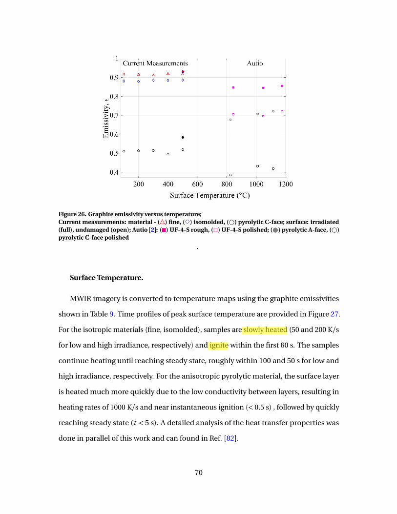
Figure 26. Graphite emissivity versus temperature;Current measurements: material - (4) fine, (3) isomolded, (#) pyrolytic C-face; surface: irradiated(full), undamaged (open); Autio [2]: (�) UF-4-S rough, (2) UF-4-S polished; ( ) pyrolytic A-face, (#)pyrolytic C-face polished
.
Surface Temperature.
MWIR imagery is converted to temperature maps using the graphite emissivities
shown in Table 9. Time profiles of peak surface temperature are provided in Figure 27.
For the isotropic materials (fine, isomolded), samples are slowly heated (50 and 200 K/s
for low and high irradiance, respectively) and ignite within the first 60 s. The samples
continue heating until reaching steady state, roughly within 100 and 50 s for low and
high irradiance, respectively. For the anisotropic pyrolytic material, the surface layer
is heated much more quickly due to the low conductivity between layers, resulting in
heating rates of 1000 K/s and near instantaneous ignition (< 0.5 s) , followed by quickly
reaching steady state (t < 5 s). A detailed analysis of the heat transfer properties was
done in parallel of this work and can found in Ref. [82].
70
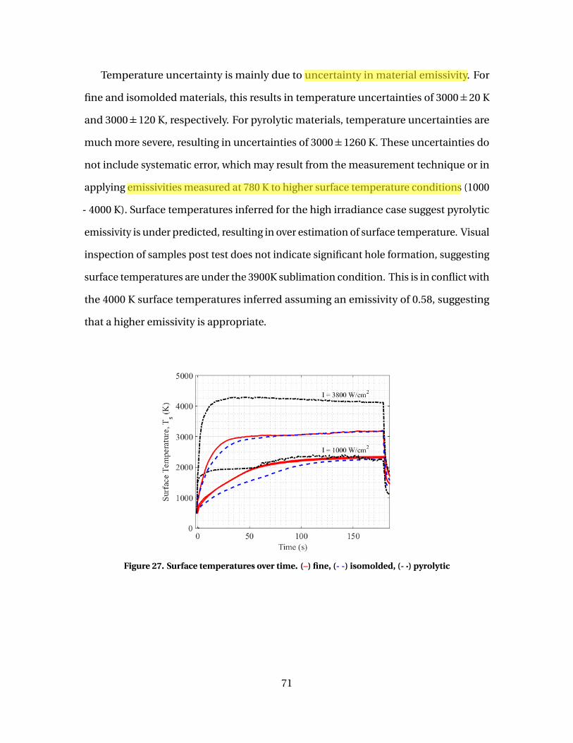
Temperature uncertainty is mainly due to uncertainty in material emissivity. For
fine and isomolded materials, this results in temperature uncertainties of 3000±20 K
and 3000±120 K, respectively. For pyrolytic materials, temperature uncertainties are
much more severe, resulting in uncertainties of 3000±1260 K. These uncertainties do
not include systematic error, which may result from the measurement technique or in
applying emissivities measured at 780 K to higher surface temperature conditions (1000
- 4000 K). Surface temperatures inferred for the high irradiance case suggest pyrolytic
emissivity is under predicted, resulting in over estimation of surface temperature. Visual
inspection of samples post test does not indicate significant hole formation, suggesting
surface temperatures are under the 3900K sublimation condition. This is in conflict with
the 4000 K surface temperatures inferred assuming an emissivity of 0.58, suggesting
that a higher emissivity is appropriate.
Figure 27. Surface temperatures over time. (–) fine, (- -) isomolded, (- ·) pyrolytic
71

Plume Properties.
IFTS hyperspectral imagery was used to infer plume temperature and species con-
centration. Plume spectra are time averaged over the relatively steady region, from
t = 100 - 150 s. Sample spectrum from a single pixel of a hyperspectral datacube is
shown Figure 28. Measured spectra was fit using the RTM given in Eq. (142). Simulated
emissivities and path transmission are also shown. Modeled spectra is in good agree-
ment with measured data, with the exception of the 2250 - 2400 cm-1 region where path
transmission features dominate, highlighting the limitations of the two layer model.
Despite these issues, good fits of the fine C O structure and broad C O2 feature outside of
the atmospheric absorption region still allow good estimation of the plume properties.
The simulated fits results in plume values of Tp l ume = 2240 ± 40 K, XC O2= 0.112 ± 0.004,
and XC O = 0.26 ± 0.03, where error bounds represent the 95% confidence interval and
do not include systematic error. Systematic errors of <6 % for plume temperature and
5-21 % for species mole fraction are estimated (see Appendix B). The largest source of
systematic error is the choice of flame length, which directly influences X i . Reported
mole fractions assume a constant flame length of 2 cm across all lines of sight.
Full spatial maps are produced by fitting all pixels in the hyperspectral data cube
using a nonlinear fitting routine. Plume maps are shown in Figure 29 for an isomolded
samples irradiated at 1000 and 3600 W/cm2. The beam is incident horizontally, centered
at y = 0 with a radius of 7 mm. The high surface temperatures within the beam activates
surface oxidation, producing C O at the surface. As the C O diffuses away, it reacts with
the available O2 producing C O2 in the exothermic C O oxidation. The discontinuity
seen in the 1000 W/cm2 case near laser center is due to slight angling of the sample
surface. Comparing the high and low irradiance case, higher surface temperatures
for the 3600 W/cm2 case result in higher C O at the surface, with XC O of 0.33 and 0.12
for the high and low irradiance, respectively. The increase in C O population allowed
72
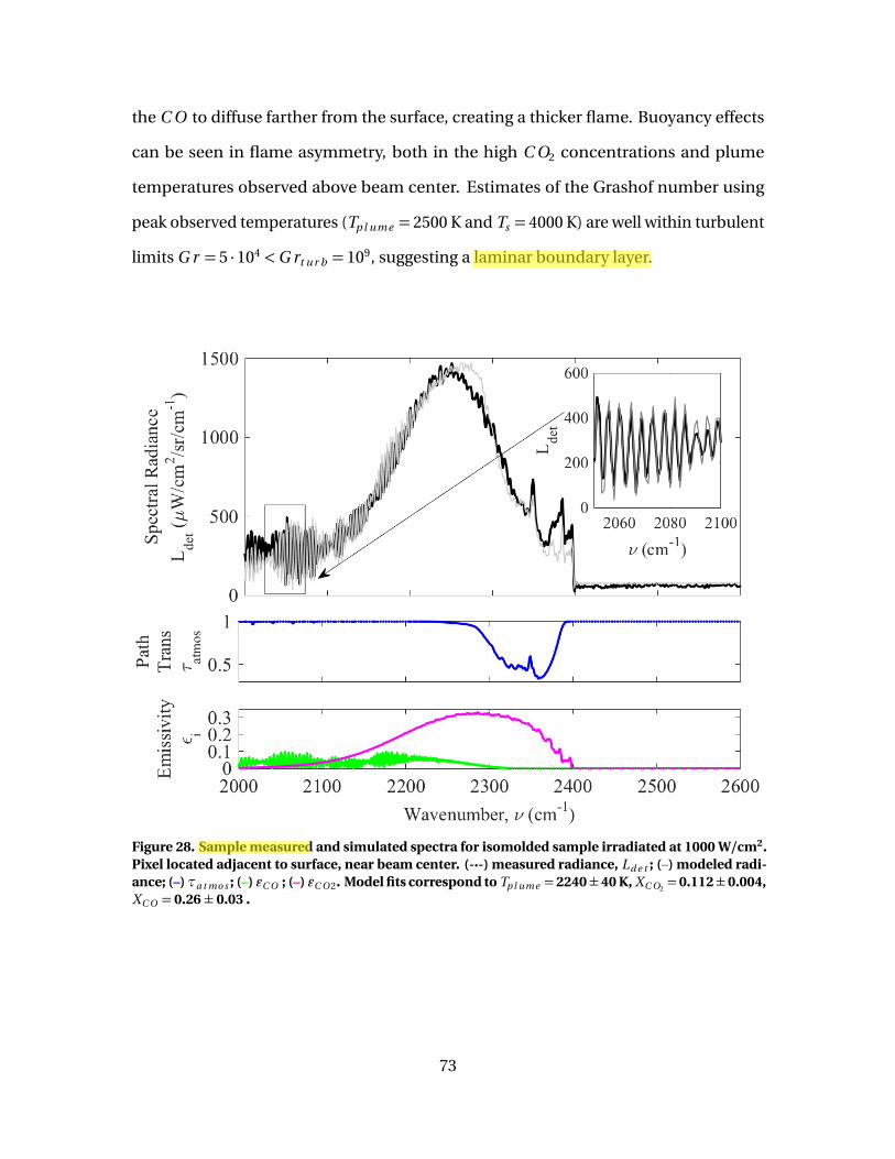
the C O to diffuse farther from the surface, creating a thicker flame. Buoyancy effects
can be seen in flame asymmetry, both in the high C O2 concentrations and plume
temperatures observed above beam center. Estimates of the Grashof number using
peak observed temperatures (Tp l ume = 2500 K and Ts = 4000 K) are well within turbulent
limits G r = 5 ·104 <G rt u r b = 109, suggesting a laminar boundary layer.
Figure 28. Sample measured and simulated spectra for isomolded sample irradiated at 1000 W/cm2.Pixel located adjacent to surface, near beam center. (-·-) measured radiance, Ld e t ; (–) modeled radi-ance; (–)τa t mo s ; (–) εC O ; (–) εC O 2. Model fits correspond to Tp l ume = 2240± 40 K, XC O2
= 0.112± 0.004,XC O = 0.26 ± 0.03 .
73

(a) I = 1000 W/cm2
(b) I = 3600 W/cm2
Figure 29. Plume temperature and species mole fractions, X i , inferred from Telops data, isomoldedsample irradiated at 1000 W/cm2 and 3600 W/cm2.
74
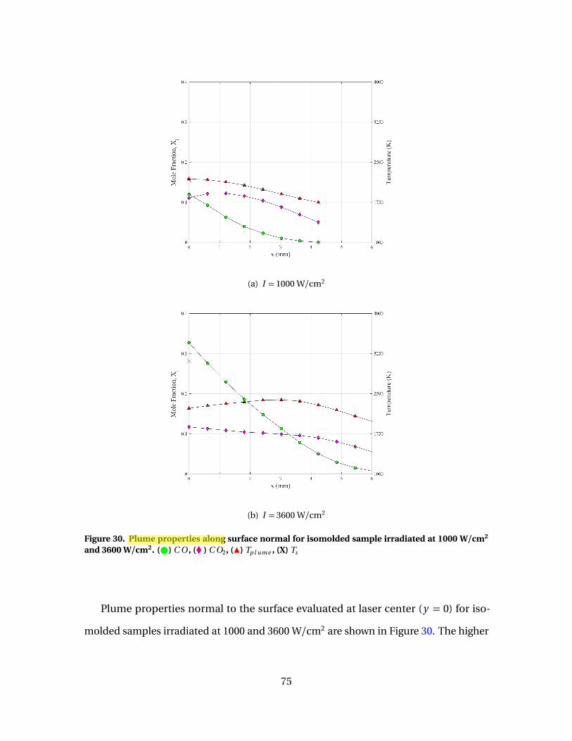
(a) I = 1000 W/cm2
(b) I = 3600 W/cm2
Figure 30. Plume properties along surface normal for isomolded sample irradiated at 1000 W/cm2
and 3600 W/cm2. ( ) C O , (� ) C O2, (Î) Tp l ume , (X) Ts
Plume properties normal to the surface evaluated at laser center (y = 0) for iso-
molded samples irradiated at 1000 and 3600 W/cm2 are shown in Figure 30. The higher
75
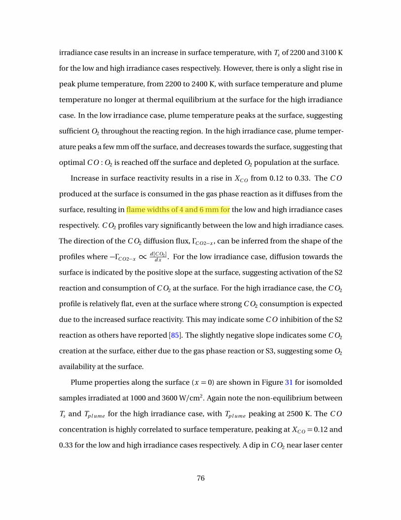
irradiance case results in an increase in surface temperature, with Ts of 2200 and 3100 K
for the low and high irradiance cases respectively. However, there is only a slight rise in
peak plume temperature, from 2200 to 2400 K, with surface temperature and plume
temperature no longer at thermal equilibrium at the surface for the high irradiance
case. In the low irradiance case, plume temperature peaks at the surface, suggesting
sufficient O2 throughout the reacting region. In the high irradiance case, plume temper-
ature peaks a few mm off the surface, and decreases towards the surface, suggesting that
optimal C O : O2 is reached off the surface and depleted O2 population at the surface.
Increase in surface reactivity results in a rise in XC O from 0.12 to 0.33. The C O
produced at the surface is consumed in the gas phase reaction as it diffuses from the
surface, resulting in flame widths of 4 and 6 mm for the low and high irradiance cases
respectively. C O2 profiles vary significantly between the low and high irradiance cases.
The direction of the C O2 diffusion flux, ΓC O 2−x , can be inferred from the shape of the
profiles where −ΓC O 2−x ∝d [C O2]
d x . For the low irradiance case, diffusion towards the
surface is indicated by the positive slope at the surface, suggesting activation of the S2
reaction and consumption of C O2 at the surface. For the high irradiance case, the C O2
profile is relatively flat, even at the surface where strong C O2 consumption is expected
due to the increased surface reactivity. This may indicate some C O inhibition of the S2
reaction as others have reported [85]. The slightly negative slope indicates some C O2
creation at the surface, either due to the gas phase reaction or S3, suggesting some O2
availability at the surface.
Plume properties along the surface (x = 0) are shown in Figure 31 for isomolded
samples irradiated at 1000 and 3600 W/cm2. Again note the non-equilibrium between
Ts and Tp l ume for the high irradiance case, with Tp l ume peaking at 2500 K. The C O
concentration is highly correlated to surface temperature, peaking at XC O = 0.12 and
0.33 for the low and high irradiance cases respectively. A dip in C O2 near laser center
76
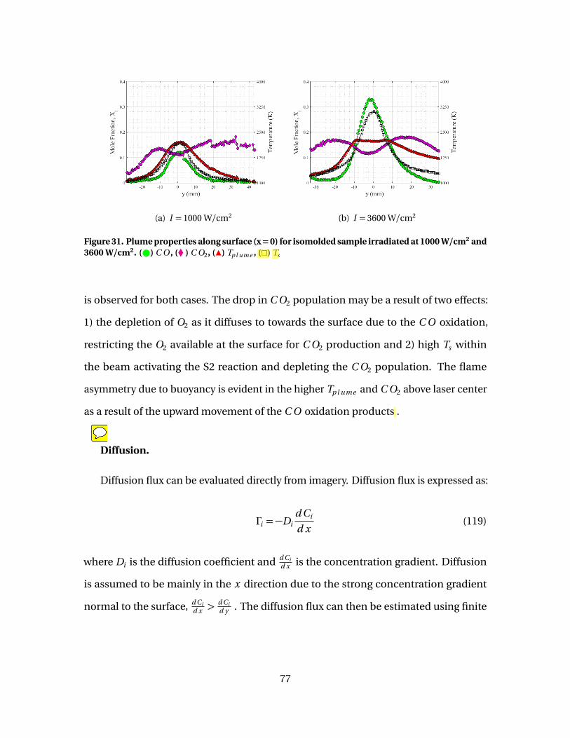
(a) I = 1000 W/cm2 (b) I = 3600 W/cm2
Figure 31. Plume properties along surface (x=0) for isomolded sample irradiated at 1000 W/cm2 and3600 W/cm2. ( ) C O , (� ) C O2, (Î) Tp l ume , (�) Ts
is observed for both cases. The drop in C O2 population may be a result of two effects:
1) the depletion of O2 as it diffuses to towards the surface due to the C O oxidation,
restricting the O2 available at the surface for C O2 production and 2) high Ts within
the beam activating the S2 reaction and depleting the C O2 population. The flame
asymmetry due to buoyancy is evident in the higher Tp l ume and C O2 above laser center
as a result of the upward movement of the C O oxidation products .
Diffusion.
Diffusion flux can be evaluated directly from imagery. Diffusion flux is expressed as:
Γi =−Di
d Ci
d x(119)
where Di is the diffusion coefficient and d Cid x is the concentration gradient. Diffusion
is assumed to be mainly in the x direction due to the strong concentration gradient
normal to the surface, d Cid x >
d Cid y . The diffusion flux can then be estimated using finite
77
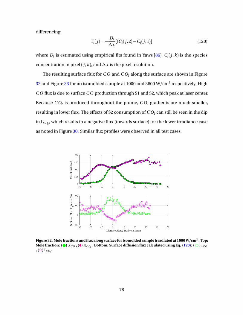
differencing:
Γi ( j ) =−Di
∆x[(Ci ( j , 2)−Ci ( j , 1)] (120)
where Di is estimated using empirical fits found in Yaws [86], Ci ( j , k ) is the species
concentration in pixel ( j , k ), and∆x is the pixel resolution.
The resulting surface flux for C O and C O2 along the surface are shown in Figure
32 and Figure 33 for an isomolded sample at 1000 and 3600 W/cm2 respectively. High
C O flux is due to surface C O production through S1 and S2, which peak at laser center.
Because C O2 is produced throughout the plume, C O2 gradients are much smaller,
resulting in lower flux. The effects of S2 consumption of C O2 can still be seen in the dip
in ΓC O2, which results in a negative flux (towards surface) for the lower irradiance case
as noted in Figure 30. Similar flux profiles were observed in all test cases.
Figure 32. Mole fractions and flux along surface for isomolded sample irradiated at 1000 W/cm2 . Top:Mole fraction: ( ) XC O , (�) XC O2
; Bottom: Surface diffusion flux calculated using Eq. (120): (# ) ΓC O
, (3) ΓC O2.
78
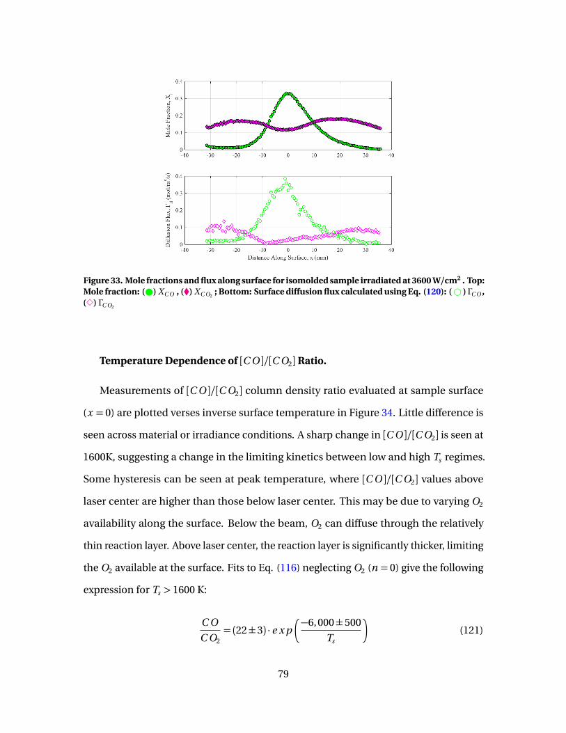
Figure 33. Mole fractions and flux along surface for isomolded sample irradiated at 3600 W/cm2 . Top:Mole fraction: ( ) XC O , (�) XC O2
; Bottom: Surface diffusion flux calculated using Eq. (120): (# ) ΓC O ,(3) ΓC O2
Temperature Dependence of [C O ]/[C O2] Ratio.
Measurements of [C O ]/[C O2] column density ratio evaluated at sample surface
(x = 0) are plotted verses inverse surface temperature in Figure 34. Little difference is
seen across material or irradiance conditions. A sharp change in [C O ]/[C O2] is seen at
1600K, suggesting a change in the limiting kinetics between low and high Ts regimes.
Some hysteresis can be seen at peak temperature, where [C O ]/[C O2] values above
laser center are higher than those below laser center. This may be due to varying O2
availability along the surface. Below the beam, O2 can diffuse through the relatively
thin reaction layer. Above laser center, the reaction layer is significantly thicker, limiting
the O2 available at the surface. Fits to Eq. (116) neglecting O2 (n = 0) give the following
expression for Ts > 1600 K:
C O
C O2= (22±3) · e x p
�−6, 000±500
Ts
�
(121)
79
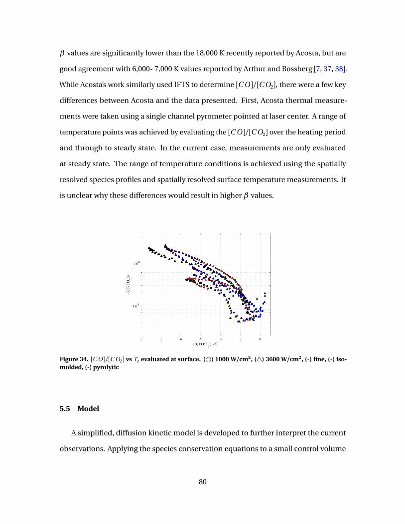
β values are significantly lower than the 18,000 K recently reported by Acosta, but are
good agreement with 6,000- 7,000 K values reported by Arthur and Rossberg [7, 37, 38].
While Acosta’s work similarly used IFTS to determine [C O ]/[C O2], there were a few key
differences between Acosta and the data presented. First, Acosta thermal measure-
ments were taken using a single channel pyrometer pointed at laser center. A range of
temperature points was achieved by evaluating the [C O ]/[C O2] over the heating period
and through to steady state. In the current case, measurements are only evaluated
at steady state. The range of temperature conditions is achieved using the spatially
resolved species profiles and spatially resolved surface temperature measurements. It
is unclear why these differences would result in higher β values.
Figure 34. [C O ]/[C O2] vs Ts evaluated at surface. (#) 1000 W/cm2, (4) 3600 W/cm2, (-) fine, (-) iso-molded, (-) pyrolytic
5.5 Model
A simplified, diffusion kinetic model is developed to further interpret the current
observations. Applying the species conservation equations to a small control volume
80
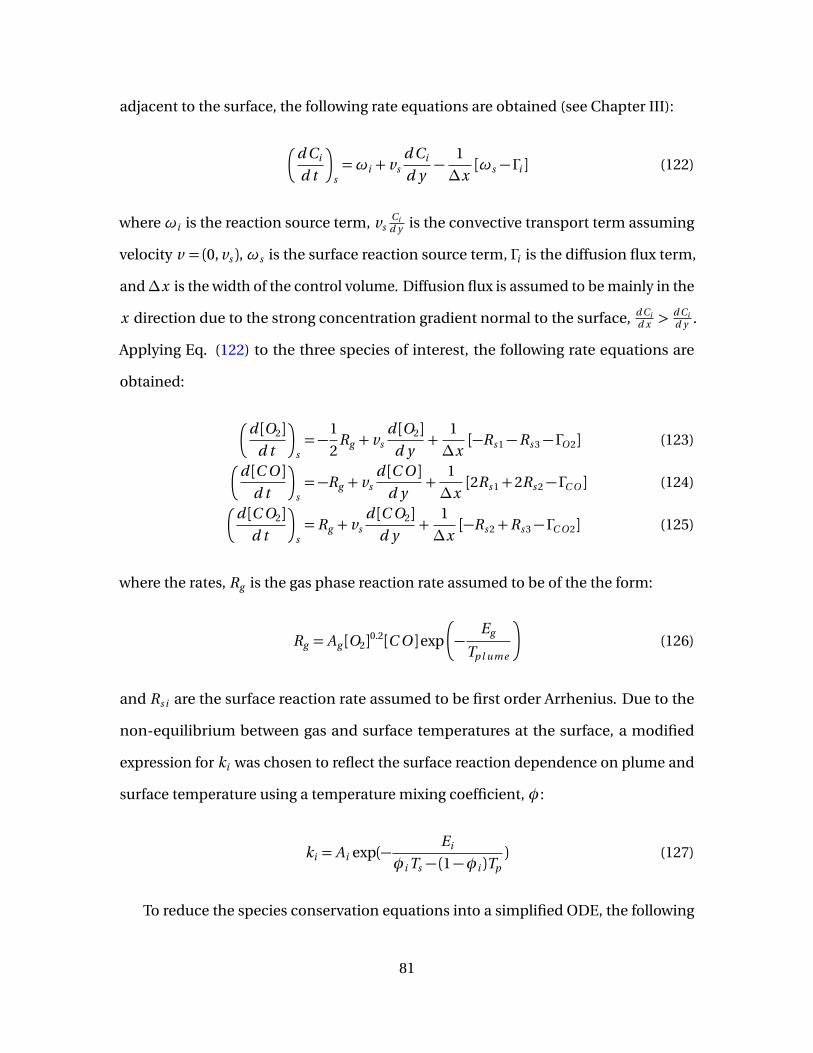
adjacent to the surface, the following rate equations are obtained (see Chapter III):
�
d Ci
d t
�
s=ωi + vs
d Ci
d y−
1
∆x[ωs − Γi ] (122)
whereωi is the reaction source term, vsCid y is the convective transport term assuming
velocity v = (0, vs ),ωs is the surface reaction source term, Γi is the diffusion flux term,
and∆x is the width of the control volume. Diffusion flux is assumed to be mainly in the
x direction due to the strong concentration gradient normal to the surface, d Cid x >
d Cid y .
Applying Eq. (122) to the three species of interest, the following rate equations are
obtained:
�
d [O2]d t
�
s=−
1
2Rg + vs
d [O2]d y
+1
∆x[−Rs 1−Rs 3− ΓO 2] (123)
�
d [C O ]d t
�
s=−Rg + vs
d [C O ]d y
+1
∆x[2Rs 1+2Rs 2− ΓC O ] (124)
�
d [C O2]d t
�
s=Rg + vs
d [C O2]d y
+1
∆x[−Rs 2+Rs 3− ΓC O 2] (125)
where the rates, Rg is the gas phase reaction rate assumed to be of the the form:
Rg = Ag [O2]0.2[C O ]exp
�
−Eg
Tp l ume
�
(126)
and Rs i are the surface reaction rate assumed to be first order Arrhenius. Due to the
non-equilibrium between gas and surface temperatures at the surface, a modified
expression for ki was chosen to reflect the surface reaction dependence on plume and
surface temperature using a temperature mixing coefficient,φ:
ki = Ai exp(−Ei
φi Ts − (1−φi )Tp) (127)
To reduce the species conservation equations into a simplified ODE, the following
81
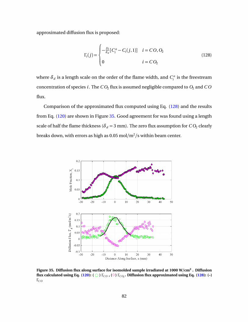
approximated diffusion flux is proposed:
Γi ( j ) =
−Diδd[C o
i −Ci ( j , 1)] i =C O , O2
0 i =C O2
(128)
where δd is a length scale on the order of the flame width, and C oi is the freestream
concentration of species i . The C O2 flux is assumed negligible compared to O2 and C O
flux.
Comparison of the approximated flux computed using Eq. (128) and the results
from Eq. (120) are shown in Figure 35. Good agreement for was found using a length
scale of half the flame thickness (δd = 3 mm). The zero flux assumption for C O2 clearly
breaks down, with errors as high as 0.05 mol/m2/s within beam center.
Figure 35. Diffusion flux along surface for isomolded sample irradiated at 1000 W/cm2 . Diffusionflux calculated using Eq. (120): (# ) ΓC O , (3) ΓC O2
. Diffusion flux approximated using Eq. (128): (–)ΓC O
82
Combining Eq. (123) - (128) and assuming steady state, results in a system of three
first order ODEs. Boundary conditions are provided by the upstream conditions, which
are assumed to be the free stream values (X oO 2 = 0.2, X o
C O = 0, and X oC O2= 0). Due to
nonlinearity and the coupling of the ODEs, a numerical solver is used. A nonlinear
least squares fitting routine is used to determine reaction rate parameters necessary for
agreement between simulated C O and C O2 profiles and experimental observations.
Surface reaction rates are controlled through fitting of Ai and Ei , which were allowed to
vary from sample to sample. Gas phase reaction rates where controlled through fitting
of Ag , which was then fixed based on best fit of the six test cases.
5.6 Model Results and Discussion
Sample fit results are shown in Figure 36 for isomolded samples irradiated at 3600
W/cm2. Fits to rate parameters are achieved using a nonlinear fitting routine comparing
simulated species profiles to experimental data. Reaction rates are computed using the
experimental temperature profiles given in the top portion of the figure, with surface
temperatures of 1400 - 3000 K. Simulated reaction rates are shown in the middle portion
of the figure along with C O transport mechanisms. The resulting simulated species
profiles are compared with measured profiles in the bottom portion of the figure. Good
agreement is found between measured and simulated concentration profiles, with
normalized root mean squared error (RMSE) of 4%.
These results allow us to infer some information about the balance of kinetic and
transport mechanisms. For the C O2 population, there is clearly a balance between
C O2 consumption through S2 and production through the gas phase reaction. For the
C O population, C O production is clearly dominated by the S1 reaction, with some
contribution from the S2 reaction. Due to the low flow velocities, contributions from
convective transport are significantly lower than diffusion transport. This suggests
83
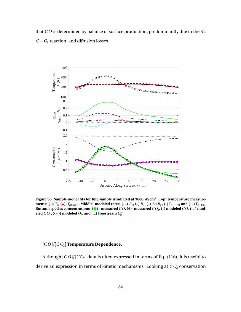
that C O is determined by balance of surface production, predominantly due to the S1:
C −O2 reaction, and diffusion losses.
Figure 36. Sample model fits for fine sample irradiated at 3600 W/cm2. Top: temperature measure-ments: (�) Ts , (Î)-Tp l ume , Middle: modeled rates: (- -) R1, (–) R2, (–)∆x Rg , (–) Γd−C O , and (- -) Γc−C O .Bottom: species concentrations- ( ) - measured C O , (�)- measured C O2, (–) modeled C O , (-.-) mod-eled C O2, (- - -) modeled O2, and (...) freestream O o
2
[C O ]/[C O2] Temperature Dependence.
Although [C O ]/[C O2] data is often expressed in terms of Eq. (116), it is useful to
derive an expression in terms of kinetic mechanisms. Looking at C O2 conservation
84
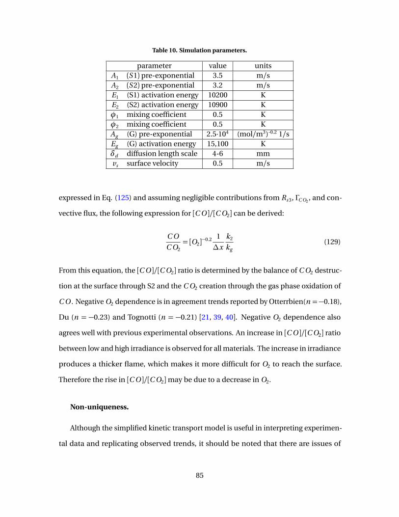
Table 10. Simulation parameters.
parameter value unitsA1 (S1) pre-exponential 3.5 m/sA2 (S2) pre-exponential 3.2 m/sE1 (S1) activation energy 10200 KE2 (S2) activation energy 10900 Kφ1 mixing coefficient 0.5 Kφ2 mixing coefficient 0.5 KAg (G) pre-exponential 2.5·104 (mol/m3)-0.2 1/sEg (G) activation energy 15,100 Kδd diffusion length scale 4-6 mmvs surface velocity 0.5 m/s
expressed in Eq. (125) and assuming negligible contributions from Rs 3, ΓC O2, and con-
vective flux, the following expression for [C O ]/[C O2] can be derived:
C O
C O2= [O2]
−0.2 1
∆x
k2
kg(129)
From this equation, the [C O ]/[C O2] ratio is determined by the balance of C O2 destruc-
tion at the surface through S2 and the C O2 creation through the gas phase oxidation of
C O . Negative O2 dependence is in agreement trends reported by Otterrbien(n =−0.18),
Du (n = −0.23) and Tognotti (n = −0.21) [21, 39, 40]. Negative O2 dependence also
agrees well with previous experimental observations. An increase in [C O ]/[C O2] ratio
between low and high irradiance is observed for all materials. The increase in irradiance
produces a thicker flame, which makes it more difficult for O2 to reach the surface.
Therefore the rise in [C O ]/[C O2]may be due to a decrease in O2.
Non-uniqueness.
Although the simplified kinetic transport model is useful in interpreting experimen-
tal data and replicating observed trends, it should be noted that there are issues of
85
non-uniqueness present in the model with prevent determining exact values for kinetic
rate parameters. Central to this issue is the choice of Ag . Take Eq. (125), assuming
steady state, negligible convection and diffusion, and negligible contribution of the S3
reaction:
∆x kg [C O ][O2]0.2 = k2[C O2] (130)
which states that C O2 created in the gas phase is balanced by the consumption of
the S2 reaction. This highlights the coupling of kg and k2 terms, meaning choice of
Ag directly determines A2. Choice of A2 then influences S1 parameters through the
coupling of S1 and S2 through the C O conservation equations. As values of Ag can vary
by orders of magnitude in literature, it is then difficult to infer exact values for kinetic
rate parameters.
5.7 Conclusions
The oxidation of laser irradiated graphite in buoyant flow has been characterized
for three graphite materials at surface temperatures of 1500-3100 K. Spatial maps of
C O , C O2, and Tp l ume are obtained using IFTS. Plume temperatures were found to be
in non-equilibrium with surface temperatures, peaking at 2500 K. C O population is
found to be highly correlated with surface temperature due to production through S1
and S2 surface reactions. C O2 populations were found to decrease at laser center due
to the S2 reaction. A general trend of [C O ]/[C O2] = 22exp(−6000/Ts ) is reported for
Ts = 1600-3100. Little difference between graphite material is noted.
A simplified species conservation model, incorporating kinetics and diffusion, is
presented to interpret experimental observations. A nonlinear fit routine comparing
simulated and measured species profiles is used to determine the relative strengths
of surface reactions. Results suggest C O population controlled by balance between
production at the surface, predominantly through the S1: Cs −O2 => 2C O reaction,
86
and diffusion away from the surface. Results also indicate C O2 population is controlled
by the balance between consumption at the surface through S2: Cs −C O2 => 2C O and
production through the gas phase reaction, suggesting the contributions from the S3:
Cs −O2 =>C O2 reaction are negligible.
While the model presented provides insight into the relative contributions of kinetic
and transport terms, several limitations should be discussed. First, the coupling of ki-
netic mechanisms presents an issue of non-uniqueness, making it difficult to accurately
determine rate parameters. This may be improved through a set of experiments to
decouple these parameters, such as graphite oxidation in C O2/N2 which would isolate
the S2 reaction from any O2 mechanisms. Second, this model greatly over simplifies
transport and kinetic mechanisms. In the case of kinetics, the use of Arrhenius rate
expressions greatly reduces the computational complexity, but does not capture the in-
fluence of individual elementary reactions, many of which contribute to non-Arrhenius
behavior. Due to these issues, rate parameters used should be considered model fit
parameters and not an estimation of actual values. This technique was used simply
to gage the relative contributions of kinetic and transport mechanisms and interpret
experimental trends. This points to the need for detailed CFD simulations which not
only greatly improve transport modeling, but can also incorporate complex kinetic rate
packages.
While IFTS is an incredibly useful diagnostic, several limitations should also be
noted. First, IFTS imagery remains a line of sight measurement, and due to the nonlin-
earities of radiative transfer, the line of sight effects can be nontrivial. Second, inferred
mole fractions are highly dependent on choice of flame length due to their coupling in
optical depth (see Appendix B). Data presented in this study assumes a constant flame
length along the line of sight. Constant flame length assumption is less problematic
along the surface, where flame width is on the order of laser beam width and relatively
87

constant above laser center. However this assumption may be particularly problematic
when comparing measurements normal to the surface, where flame thickness changes
dramatically from surface to flame edge.
88
VI. Imaging Fourier Transform Spectroscopy of Graphite Oxidationin a Flat Plate Shear Flow
This chapter focuses on expanding IFTS graphite oxidation measurements to the
flat plate shear flow, in partial fulfillment of objective 1. Oxidation models, developed in
Chapter III and evaluated against buoyant flow data in Chapter V, are evaluated for the
current flow configuration, in partial fulfillment of objective 2. The chapter is written
in journal article format and can be read independently as a stand alone document.
Additional details regarding background and experimental method can be found in
Chapter II and IV, respectively.
6.1 Abstract
The oxidation of laser irradiated graphite in laminar flow is characterized using
imaging Fourier transform spectroscopy (IFTS). Samples of varying porosity are irra-
diated using a 1.07 µm fiber laser at irradiances of 750 and 1500 W/cm2 in a dry flow
(20% O2, < 1% H2O ) with flow speeds of 5 - 10 m/s, resulting in surface temperatures
of 1000 - 4000 K. The resulting reacting layer is observed using a midwave (MW) IFTS
at 2 cm-1 spectral resolution, 0.5 mm/pixel spatial resolution, and 0.75 Hz data cube
rate. Spectral signatures feature emission from C O and C O2 in the 1800 - 2500 cm-1
spectral region. A two layer radiative transfer model using the CDSD-4000 and HITEMP
cross-section databases was used to determine path-averaged plume temperature, C O ,
and C O2 concentrations from spectral signatures. Plume temperatures are found be in
non-equilibrium with surface temperatures, with peak plume temperatures of only 2500
K. C O and C O2 populations are highly correlated with surface and plume temperature.
A general trend of [C O ]/[C O2] = 7.8exp(−3100/Ts ) is reported for all materials. This
data set represents the first spatially resolved measurements of graphite oxidation in a
flat plate shear flow.
89
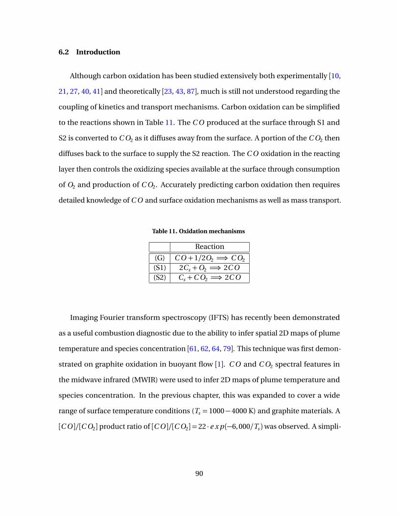
6.2 Introduction
Although carbon oxidation has been studied extensively both experimentally [10,
21, 27, 40, 41] and theoretically [23, 43, 87], much is still not understood regarding the
coupling of kinetics and transport mechanisms. Carbon oxidation can be simplified
to the reactions shown in Table 11. The C O produced at the surface through S1 and
S2 is converted to C O2 as it diffuses away from the surface. A portion of the C O2 then
diffuses back to the surface to supply the S2 reaction. The C O oxidation in the reacting
layer then controls the oxidizing species available at the surface through consumption
of O2 and production of C O2. Accurately predicting carbon oxidation then requires
detailed knowledge of C O and surface oxidation mechanisms as well as mass transport.
Table 11. Oxidation mechanisms
Reaction
(G) C O +1/2O2 =⇒ C O2
(S1) 2Cs +O2 =⇒ 2C O(S2) Cs +C O2 =⇒ 2C O
Imaging Fourier transform spectroscopy (IFTS) has recently been demonstrated
as a useful combustion diagnostic due to the ability to infer spatial 2D maps of plume
temperature and species concentration [61, 62, 64, 79]. This technique was first demon-
strated on graphite oxidation in buoyant flow [1]. C O and C O2 spectral features in
the midwave infrared (MWIR) were used to infer 2D maps of plume temperature and
species concentration. In the previous chapter, this was expanded to cover a wide
range of surface temperature conditions (Ts = 1000−4000 K) and graphite materials. A
[C O ]/[C O2] product ratio of [C O ]/[C O2] = 22 · e x p (−6, 000/Ts )was observed. A simpli-
90

fied kinetic transport model was used to interpret experimental observations and infer
the relative strengths of kinetic and transport mechanisms.
Although the simplified kinetic model is useful to interpreting experimental trends,
it is severely limited due to the over simplification of kinetics and transport mechanisms.
This highlights the need for detailed CFD simulations, which not only greatly improve
the transport modeling, but can also incorporate complex kinetic rate packages. C O
oxidation rate packages using a limited number of elementary reactions are already
in use [13]. Similar packages for graphite oxidation using a set of semiglobal reactions
have also been developed [6]. CFD simulations incorporating these kinetic models have
also been demonstrated for graphite oxidation in flat plate shear flow and stagnation
flow [8]. However, validation of this work has been difficult due to the lack of spatially
resolved experimental data in these flow regimes.
The current study expands on previous experimental work to investigate laser irradi-
ated graphite in a flat plate shear flow using IFTS. This work represents the first spatially
resolved measurements of graphite oxidation in a flat plate shear flow, which is vital for
validation of numerical work. In addition, flat plate shear flow allows observation of
graphite oxidation in a new set of transport conditions. The kinetic transport model
used in previous work is again used to interpret experimental observations. Changes in
[C O ]/[C O2] product ratio for varying surface temperature and flow rate are discussed.
6.3 Experimental
Overview.
Three graphite materials were each irradiated at 750 and 1500 W/cm2 for 120 s to
produce steady state surface temperatures of 1000 - 4000 K. Samples were tested at
the Wright-Patterson Air Force Base Laser Hardened Materials Evaluation Laboratory
(LHMEL) using a 15 kW fiber laser at 1.07 µm, which produced a 1.4±0.2 cm diame-
91
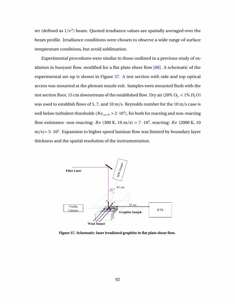
ter (defined as 1/e 2) beam. Quoted irradiance values are spatially averaged over the
beam profile. Irradiance conditions were chosen to observe a wide range of surface
temperature conditions, but avoid sublimation.
Experimental procedures were similar to those outlined in a previous study of ox-
idation in buoyant flow, modified for a flat plate sheer flow [88]. A schematic of the
experimental set-up is shown in Figure 37. A test section with side and top optical
access was mounted at the plenum nozzle exit. Samples were mounted flush with the
test section floor, 15 cm downstream of the established flow. Dry air (20% O2,< 1% H2O )
was used to establish flows of 5, 7, and 10 m/s. Reynolds number for the 10 m/s case is
well below turbulent thresholds (R et u r b > 2 ·105), for both for reacting and non-reacting
flow estimates: non-reacting: R e (300 K, 10 m/s) = 7 · 104, reacting: R e (2000 K, 10
m/s)= 3 ·103. Expansion to higher speed laminar flow was limited by boundary layer
thickness and the spatial resolution of the instrumentation.
Figure 37. Schematic: laser irradiated graphite in flat plate shear flow.
92
Materials .
Material properties of the three Graphtek graphite materials are shown in Table 12 [3].
The isomolded and fine samples are produced through an isostatic press and extrusion
methods respectively. Impurities found in the ash content are not reported by the
manufacturer, but previous work with fine samples report observations of Si, S, Fe, Ca,
Al, and K [58]. Additionally these production methods make use of a more reactive binder
material, which can react at much lower temperatures, increasing porosity [58, 78]. The
pyrolytic material is produced in a layering method, which produces high purity samples
with negligible porosity. The layering method results in high conductivity within the
layers, but little conductivity between layers. Samples are cut such that the sample
surface is a single layer (C-face). Additional details on graphite materials, impurities, as
well as sample photographs can be found in [58].
Emissivities provided for the three materials are based on measurements of post
irradiated samples [82, 88]. Although graphite emissivities have been previously shown
to be relatively insensitive to surface temperature, emissivity can vary significantly by
graphite type and surface condition [2]. Emissivities of the isomolded and fine materials
are relatively high and increase slightly with surface damage as irradiated (6− 7%).
Previous pyrolytic measurements have shown emissivities to be very anisotropic and
sensitive to surface condition. Emissivities of the C-face can vary from 0.54 (undamaged)
to 0.58 (irradiated) [88]. Additionally, A-face (layer edge) measurements have shown
emissivities as high as 0.90 [88]. Although current measurements are taken normal to
the surface (C-face), as the surface is irradiated and layers are eroded, emissivity values
may go as high as A-face values.
93
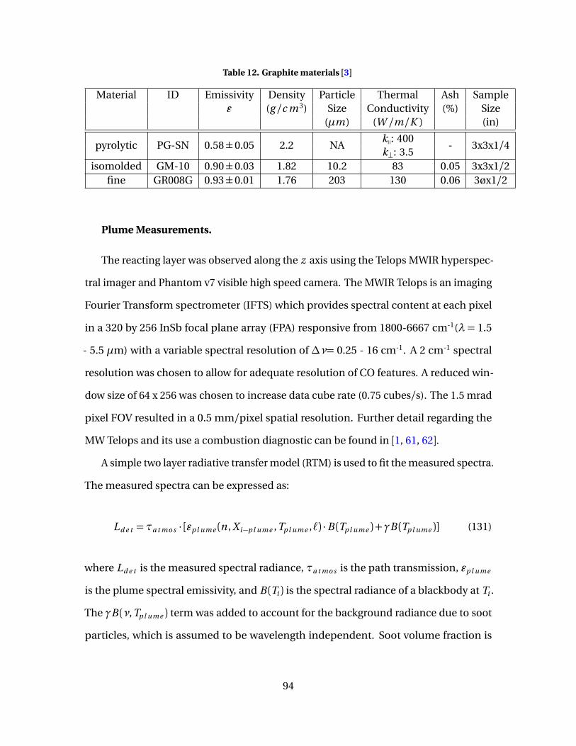
Table 12. Graphite materials [3]
Material ID Emissivity Density Particle Thermal Ash Sampleε (g /c m 3) Size Conductivity (%) Size
(µm) (W /m/K ) (in)
pyrolytic PG-SN 0.58±0.05 2.2 NAkq: 400
- 3x3x1/4k⊥: 3.5
isomolded GM-10 0.90±0.03 1.82 10.2 83 0.05 3x3x1/2fine GR008G 0.93±0.01 1.76 203 130 0.06 3øx1/2
Plume Measurements.
The reacting layer was observed along the z axis using the Telops MWIR hyperspec-
tral imager and Phantom v7 visible high speed camera. The MWIR Telops is an imaging
Fourier Transform spectrometer (IFTS) which provides spectral content at each pixel
in a 320 by 256 InSb focal plane array (FPA) responsive from 1800-6667 cm-1(λ = 1.5
- 5.5 µm) with a variable spectral resolution of ∆ν= 0.25 - 16 cm-1. A 2 cm-1 spectral
resolution was chosen to allow for adequate resolution of CO features. A reduced win-
dow size of 64 x 256 was chosen to increase data cube rate (0.75 cubes/s). The 1.5 mrad
pixel FOV resulted in a 0.5 mm/pixel spatial resolution. Further detail regarding the
MW Telops and its use a combustion diagnostic can be found in [1, 61, 62].
A simple two layer radiative transfer model (RTM) is used to fit the measured spectra.
The measured spectra can be expressed as:
Ld e t =τa t mo s · [εp l ume (n , X i−p l ume , Tp l ume ,`) ·B (Tp l ume ) +γB (Tp l ume )] (131)
where Ld e t is the measured spectral radiance, τa t mo s is the path transmission, εp l ume
is the plume spectral emissivity, and B (Ti ) is the spectral radiance of a blackbody at Ti .
The γB (ν, Tp l ume ) term was added to account for the background radiance due to soot
particles, which is assumed to be wavelength independent. Soot volume fraction is
94
low, with the γB (Tp l ume ) term accounting for less than 10 µW/cm2/sr/cm-1 of the signal.
Assuming equilibrium, emissivity can be written in terms of transmissivity (ε = 1−τ),
with transmissivity defined by Beer’s law:
τ= exp(−nl∑
k
Xkσk (ν, Tp l ume )) (132)
where n is the number density, l is the path length, Xk is the plume species mole fraction,
and σk is the species cross-section taken from HITRAN (C O , H2O ) and CDSD 4000
(C O2) databases [46, 47]. The recent addition of the CDSD 4000 high temperature C O2
cross-sections has been reported to provide much better agreement with reported C O2
signatures above 2000 K [1, 63]. A least squares fitting routine on Equation 131 is used to
infer Tp l ume , XC O , and XC O2from the spectral signatures [1, 61]. Uncertainties quoted
for plume properties are based on the 95% confidence bounds of the fit and do not
include systematic error, such as line of sight averaging and pixel blurring [88]. Full 2D
spatial maps of species concentration and plume temperature are inferred by fitting
spectra at each pixel. Further detail regarding the use of RTMs in IFTIR combustion
work can be found in Reference [62].
Thermal Measurements.
Surface temperatures were measured using the FLIR SC6000 thermal camera equipped
with a 620 by 512 FPA sensitive at 3.8-4.0 µm . The SC6000 is capable of interweaving
multiple integration times in a single test acquisition, allowing for a wider detection
range. Thermal measurements were taken using a 2.0 ND filter and integration times
of 0.1-1.5 ms, resulting in a noise floor of 500 K. Images were were taken at 10 Hz and
window size of 128x160 to reduce data volume. The FLIR was mounted 36 degrees off
normal to avoid laser path, resulting in vertical and horizontal spatial resolutions of 0.5
and 0.4 mm/pixel respectively. Raw signal is converted to temperature measurements
95
using an external blackbody (320-870 K) and calibrated using the material emissivities
[82]. The largest source of error is the uncertainty in material emissivity. At 3000 K,
emissivity uncertainties for the fine and isomolded translate to temperature uncertain-
ties of 20 and 120 K respectively. However due to the low emissivity of the pyrolytic
material, emissivity uncertainties are far more problematic, resulting in temperature
uncertainties of 3000±1260 K.
6.4 Results and Discussion
Surface Temperature.
Time profiles of peak surface temperature are shown in Figure 38. Surface tem-
peratures show little dependence on flow velocity, which is consistent with thermal
modeling efforts which find that radiative cooling and conduction to dominate heat
transfer [82]. Observations can be divided between isotropic (fine, isomolded) and
anisotropic (pyrolytic) materials. For the isotropic materials, samples are slowly heated,
26 K/s and 80-90 K/s for the low and high irradiance cases respectively, followed by
ignition once the samples reached Ts = 1450± 150 K. Steady state conditions were
reached for all cases within 80 s. For the pyrolytic samples, the low conduction between
layers causes a faster heating rate for the surface layer, resulting in heating rates of
180 K/s and 700 K/s for the low and high irradiance cases respectively. Samples ignite
quickly (t < 1 s) and reach steady state within 20 s. Inferring ignition temperatures from
pyrolytic material is difficult to uncertainties in ignition time and the high heating rates.
Temperature uncertainties are based on uncertainties in material emissivity. Surface
temperatures for the pyrolytic high irradiance case may be severely overestimated due
to the low pyrolytic emissivity and high emissivity uncertainty. Visual inspection of
samples post test does not indicate sublimation conditions, suggesting surface temper-
atures under 3900 K. It is possible that pyrolytic emissivity at higher temperatures rises
96

Figure 38. Surface temperatures over time. Material: (–) fine, (–) isomolded, (–) pyrolytic. Flow: (. .)5 m/s, (- -) 7 m/s, (–) 10 m/s.
and approaches A-face values, which would result in surface temperatures in better
agreement with those reported for fine and isomolded samples.
Plume Properties.
Telops hyperspectral data was used to infer plume temperature and species concen-
tration. Plume data is time averaged over the relatively steady region, from t = 80−100 s.
Sample spectra from a single pixel of a hyperspectral datacube is shown Figure 39. Mea-
sured spectra was fit using the RTM given in Eq. (131). The resulting simulated spectra is
shown overlayed with measured spectra. Simulation emissivities and path transmission
are also shown below. Modeled spectra is in good agreement with measured data, with
the exception of the 2250-2400 cm-1 region where path transmission features dominate,
highlighting the limitations of the two layer model. Despite these issues, good fits of
the fine C O structure and broad C O2 feature outside of the atmospheric absorption
region still allow good estimation of the plume properties (Tp l ume , C O , C O2).
Full spatial maps are produced by fitting all pixels in the hyperspectral data cube.
Plume maps are shown in Figure 40 for a fine sample irradiated at 1500 W/cm2 with 7
m/s flow. The beam is incident vertically, centered at x = 0 with a radius of 7 mm. The
97

Figure 39. Sample spectra and fit for isomolded sample irradiated at 1500 W/cm with 5 m/s flow2.(–) measured radiance, Ld e t , (–) modeled radiance, (–) path transmission, τa t mo s , (–) C O emissivity,εC O , (–) C O2 emissivity, εC O 2. Model fits correspond to Tp l ume = 2000 ± 20 K, XC O2
= 0.073 ± 0.001,XC O = 0.15 ± 0.01 .
high temperatures within the beam activates surface oxidation, producing C O at the
surface. As the C O diffuses away, it reacts with the available O2 producing C O2, which
then is transported downstream. Additional plume maps can be found in Appendix A.
98

Figure 40. Plume temperature and species mole fractions, X i , inferred from Telops data, fine sampleirradiated at 1500 W/cm2 with 7 m/s flow.
Figure 41. Plume properties normal to the surface at laser center (x = 0) for fine samples irradiatedat 1500 W/cm2 with 7 m/s flow. ( ) C O , (� ) C O2, (Î) Tp l ume , (X) Ts
99
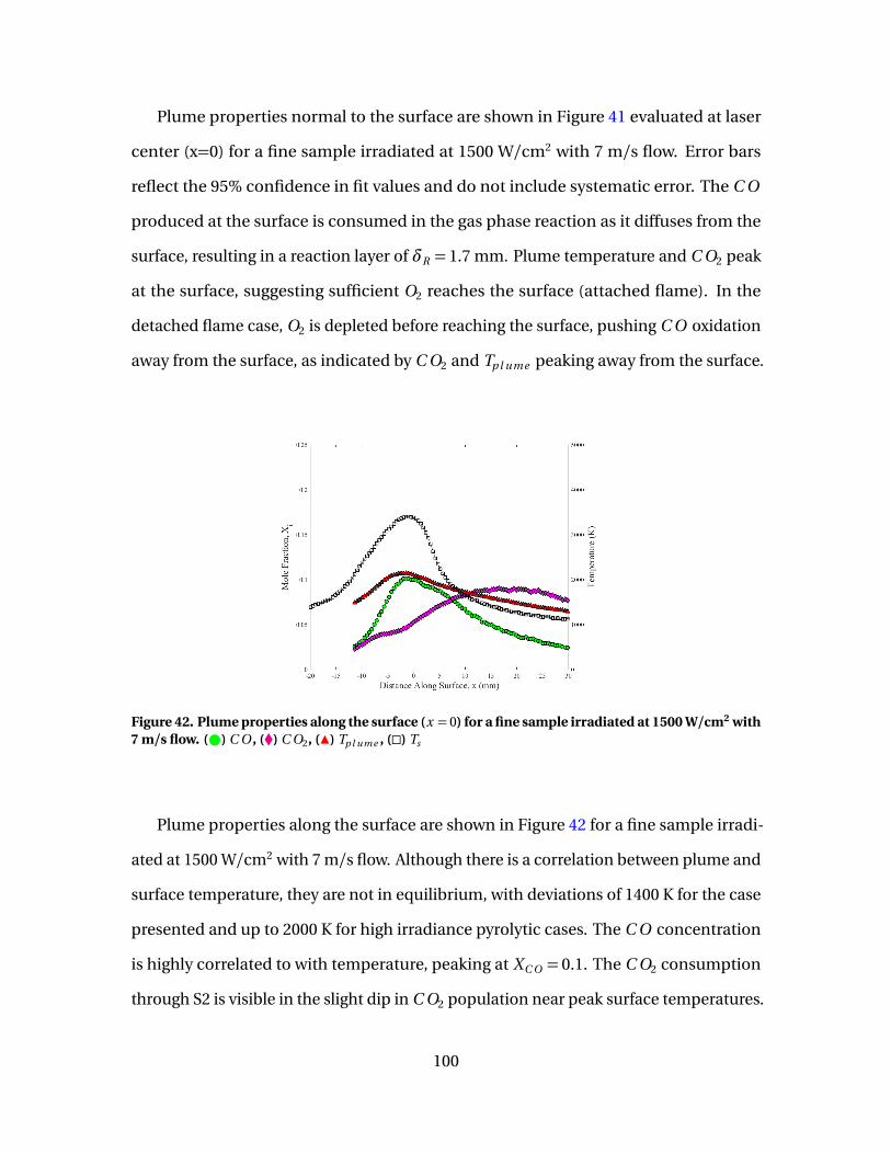
Plume properties normal to the surface are shown in Figure 41 evaluated at laser
center (x=0) for a fine sample irradiated at 1500 W/cm2 with 7 m/s flow. Error bars
reflect the 95% confidence in fit values and do not include systematic error. The C O
produced at the surface is consumed in the gas phase reaction as it diffuses from the
surface, resulting in a reaction layer of δR = 1.7 mm. Plume temperature and C O2 peak
at the surface, suggesting sufficient O2 reaches the surface (attached flame). In the
detached flame case, O2 is depleted before reaching the surface, pushing C O oxidation
away from the surface, as indicated by C O2 and Tp l ume peaking away from the surface.
Figure 42. Plume properties along the surface (x = 0) for a fine sample irradiated at 1500 W/cm2 with7 m/s flow. ( ) C O , (�) C O2, (Î) Tp l ume , (�) Ts
Plume properties along the surface are shown in Figure 42 for a fine sample irradi-
ated at 1500 W/cm2 with 7 m/s flow. Although there is a correlation between plume and
surface temperature, they are not in equilibrium, with deviations of 1400 K for the case
presented and up to 2000 K for high irradiance pyrolytic cases. The C O concentration
is highly correlated to with temperature, peaking at XC O = 0.1. The C O2 consumption
through S2 is visible in the slight dip in C O2 population near peak surface temperatures.
100
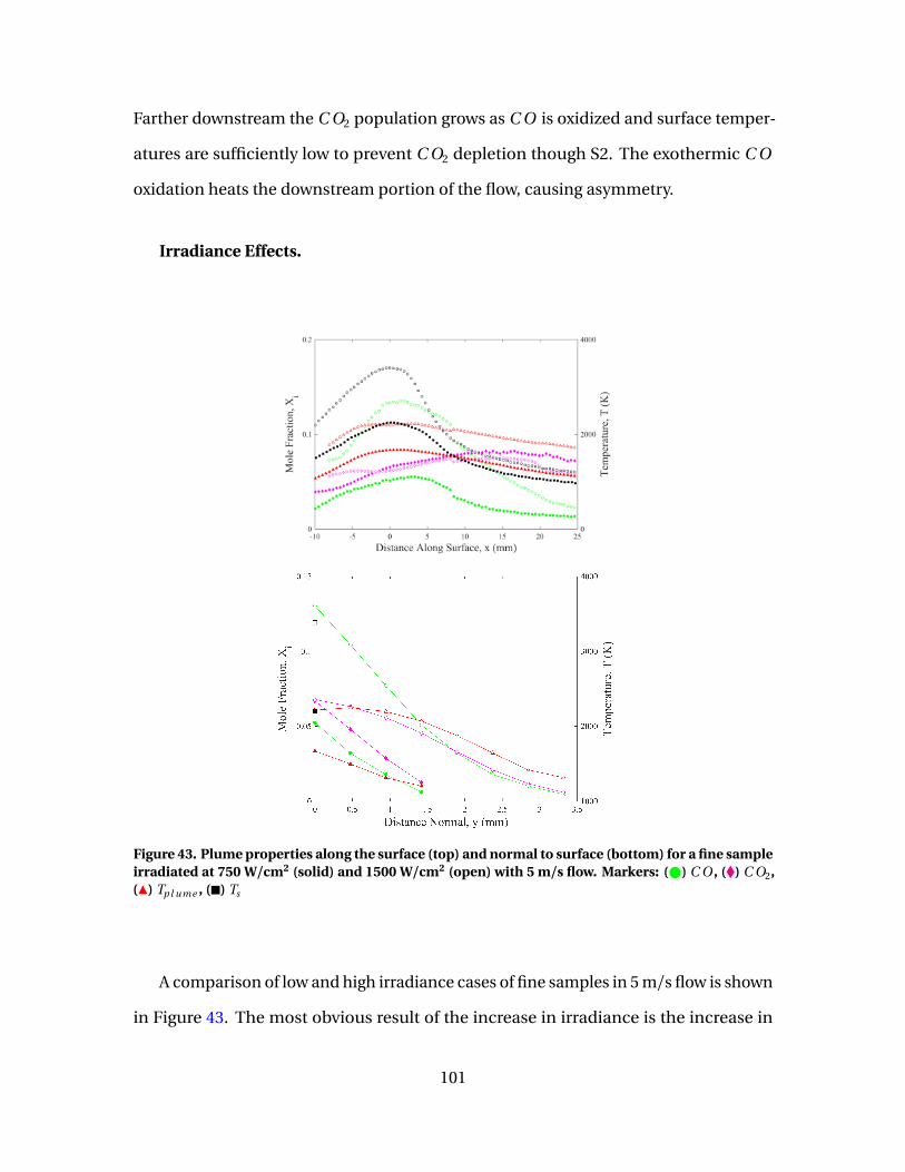
Farther downstream the C O2 population grows as C O is oxidized and surface temper-
atures are sufficiently low to prevent C O2 depletion though S2. The exothermic C O
oxidation heats the downstream portion of the flow, causing asymmetry.
Irradiance Effects.
Figure 43. Plume properties along the surface (top) and normal to surface (bottom) for a fine sampleirradiated at 750 W/cm2 (solid) and 1500 W/cm2 (open) with 5 m/s flow. Markers: ( ) C O , (�) C O2,(Î) Tp l ume , (�) Ts
A comparison of low and high irradiance cases of fine samples in 5 m/s flow is shown
in Figure 43. The most obvious result of the increase in irradiance is the increase in
101
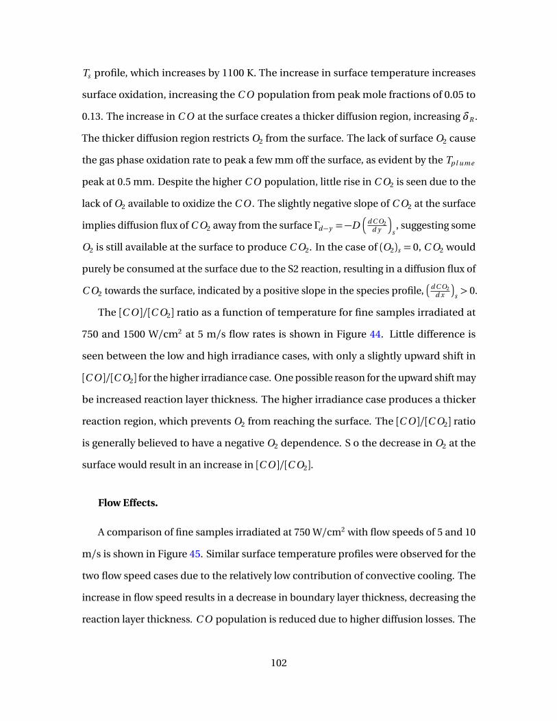
Ts profile, which increases by 1100 K. The increase in surface temperature increases
surface oxidation, increasing the C O population from peak mole fractions of 0.05 to
0.13. The increase in C O at the surface creates a thicker diffusion region, increasing δR .
The thicker diffusion region restricts O2 from the surface. The lack of surface O2 cause
the gas phase oxidation rate to peak a few mm off the surface, as evident by the Tp l ume
peak at 0.5 mm. Despite the higher C O population, little rise in C O2 is seen due to the
lack of O2 available to oxidize the C O . The slightly negative slope of C O2 at the surface
implies diffusion flux of C O2 away from the surface Γd−y =−D�
d C O2d y
�
s, suggesting some
O2 is still available at the surface to produce C O2. In the case of (O2)s = 0, C O2 would
purely be consumed at the surface due to the S2 reaction, resulting in a diffusion flux of
C O2 towards the surface, indicated by a positive slope in the species profile,�
d C O2d x
�
s> 0.
The [C O ]/[C O2] ratio as a function of temperature for fine samples irradiated at
750 and 1500 W/cm2 at 5 m/s flow rates is shown in Figure 44. Little difference is
seen between the low and high irradiance cases, with only a slightly upward shift in
[C O ]/[C O2] for the higher irradiance case. One possible reason for the upward shift may
be increased reaction layer thickness. The higher irradiance case produces a thicker
reaction region, which prevents O2 from reaching the surface. The [C O ]/[C O2] ratio
is generally believed to have a negative O2 dependence. S o the decrease in O2 at the
surface would result in an increase in [C O ]/[C O2].
Flow Effects.
A comparison of fine samples irradiated at 750 W/cm2 with flow speeds of 5 and 10
m/s is shown in Figure 45. Similar surface temperature profiles were observed for the
two flow speed cases due to the relatively low contribution of convective cooling. The
increase in flow speed results in a decrease in boundary layer thickness, decreasing the
reaction layer thickness. C O population is reduced due to higher diffusion losses. The
102
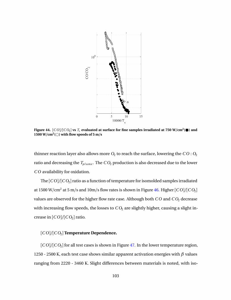
Figure 44. [C O ]/[C O2] vs Ts evaluated at surface for fine samples irradiated at 750 W/cm2( ) and1500 W/cm2(#) with flow speeds of 5 m/s
thinner reaction layer also allows more O2 to reach the surface, lowering the C O : O2
ratio and decreasing the Tp l ume . The C O2 production is also decreased due to the lower
C O availability for oxidation.
The [C O ]/[C O2] ratio as a function of temperature for isomolded samples irradiated
at 1500 W/cm2 at 5 m/s and 10m/s flow rates is shown in Figure 46. Higher [C O ]/[C O2]
values are observed for the higher flow rate case. Although both C O and C O2 decrease
with increasing flow speeds, the losses to C O2 are slightly higher, causing a slight in-
crease in [C O ]/[C O2] ratio.
[C O ]/[C O2] Temperature Dependence.
[C O ]/[C O2] for all test cases is shown in Figure 47. In the lower temperature region,
1250 - 2500 K, each test case shows similar apparent activation energies with β values
ranging from 2220 - 3460 K. Slight differences between materials is noted, with iso-
103
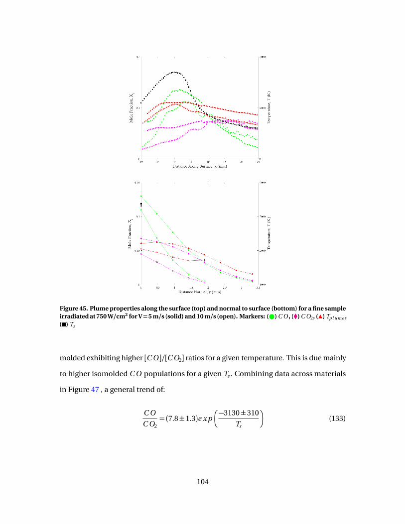
Figure 45. Plume properties along the surface (top) and normal to surface (bottom) for a fine sampleirradiated at 750 W/cm2 for V=5 m/s (solid) and 10 m/s (open). Markers: ( ) C O , (�) C O2, (Î) Tp l ume ,(�) Ts
molded exhibiting higher [C O ]/[C O2] ratios for a given temperature. This is due mainly
to higher isomolded C O populations for a given Ts . Combining data across materials
in Figure 47 , a general trend of:
C O
C O2= (7.8±1.3)e x p
�−3130±310
Ts
�
(133)
104
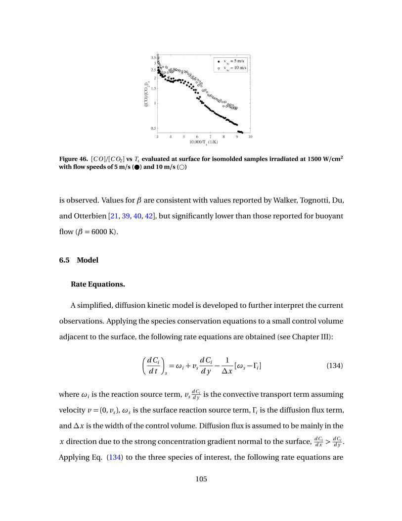
Figure 46. [C O ]/[C O2] vs Ts evaluated at surface for isomolded samples irradiated at 1500 W/cm2
with flow speeds of 5 m/s ( ) and 10 m/s (#)
is observed. Values for β are consistent with values reported by Walker, Tognotti, Du,
and Otterbien [21, 39, 40, 42], but significantly lower than those reported for buoyant
flow (β = 6000 K).
6.5 Model
Rate Equations.
A simplified, diffusion kinetic model is developed to further interpret the current
observations. Applying the species conservation equations to a small control volume
adjacent to the surface, the following rate equations are obtained (see Chapter III):
�
d Ci
d t
�
s=ωi + vs
d Ci
d y−
1
∆x[ωs − Γi ] (134)
whereωi is the reaction source term, vsd Cid y is the convective transport term assuming
velocity v = (0, vs ),ωs is the surface reaction source term, Γi is the diffusion flux term,
and∆x is the width of the control volume. Diffusion flux is assumed to be mainly in the
x direction due to the strong concentration gradient normal to the surface, d Cid x >
d Cid y .
Applying Eq. (134) to the three species of interest, the following rate equations are
105
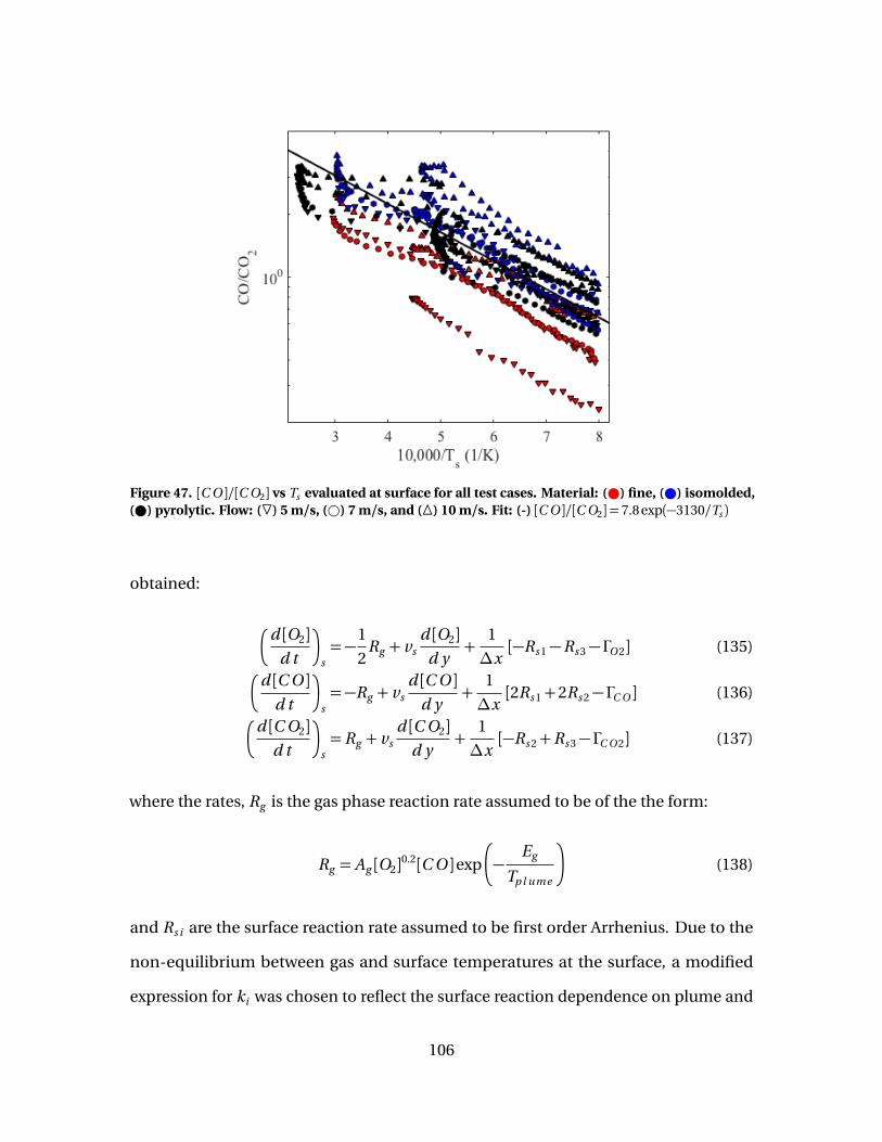
Figure 47. [C O ]/[C O2] vs Ts evaluated at surface for all test cases. Material: ( ) fine, ( ) isomolded,( ) pyrolytic. Flow: (F) 5 m/s, (#) 7 m/s, and (�) 10 m/s. Fit: (-) [C O ]/[C O2] = 7.8 exp(−3130/Ts )
obtained:
�
d [O2]d t
�
s=−
1
2Rg + vs
d [O2]d y
+1
∆x[−Rs 1−Rs 3− ΓO 2] (135)
�
d [C O ]d t
�
s=−Rg + vs
d [C O ]d y
+1
∆x[2Rs 1+2Rs 2− ΓC O ] (136)
�
d [C O2]d t
�
s=Rg + vs
d [C O2]d y
+1
∆x[−Rs 2+Rs 3− ΓC O 2] (137)
where the rates, Rg is the gas phase reaction rate assumed to be of the the form:
Rg = Ag [O2]0.2[C O ]exp
�
−Eg
Tp l ume
�
(138)
and Rs i are the surface reaction rate assumed to be first order Arrhenius. Due to the
non-equilibrium between gas and surface temperatures at the surface, a modified
expression for ki was chosen to reflect the surface reaction dependence on plume and
106
surface temperature using a temperature mixing coefficient,φ:
ki = Ai exp(−Ei
φi Ts − (1−φi )Tp) (139)
To reduce the species conservation equations into a simplified ODE, the following
approximated diffusion flux is proposed:
Γi ( j ) =
−Diδd[C o
i −Ci ( j , 1)] i =C O , O2
0 i =C O2
(140)
where δd is a length scale on the order of the flame width, and C oi is the freestream
concentration of species i . The C O2 flux is assumed negligible compared to O2 and C O
flux.
Combining Eq. (135) - (140) and assuming steady state, results in a system of three
first order ODEs. Boundary conditions are provided by the upstream conditions, which
are assumed to be the free stream values (X oO 2 = 0.2, X o
C O = 0, and X oC O2= 0). Due to
nonlinearity and the coupling of the ODEs, a numerical solver is used. A nonlinear
least squares fitting routine is used to determine reaction rate parameters necessary for
agreement between simulated C O and C O2 profiles and experimental observations.
Surface reaction rates are controlled through fitting of Ai and Ei , which were allowed to
vary from sample to sample. Gas phase reaction rates where controlled through fitting
of Ag , which was then fixed based on best fit of the six test cases.
Model Results.
A nonlinear least squares fitting routine was used to fit kinetic rate parameters to
achieve agreement between observed and simulated C O and C O2 surface profiles.
Model results for an isomolded sample irradiated at 1500 W/cm2 with 7 m/s flow are
107
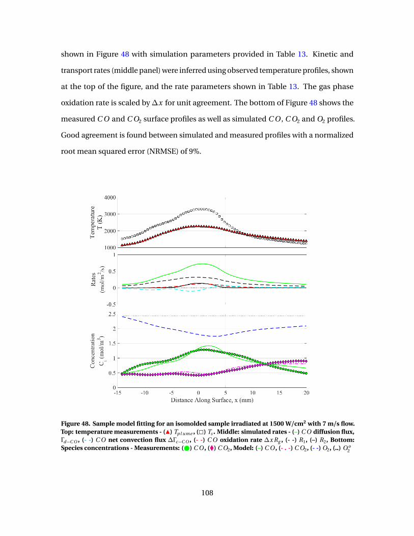
shown in Figure 48 with simulation parameters provided in Table 13. Kinetic and
transport rates (middle panel) were inferred using observed temperature profiles, shown
at the top of the figure, and the rate parameters shown in Table 13. The gas phase
oxidation rate is scaled by∆x for unit agreement. The bottom of Figure 48 shows the
measured C O and C O2 surface profiles as well as simulated C O , C O2 and O2 profiles.
Good agreement is found between simulated and measured profiles with a normalized
root mean squared error (NRMSE) of 9%.
Figure 48. Sample model fitting for an isomolded sample irradiated at 1500 W/cm2 with 7 m/s flow.Top: temperature measurements - (Î) Tp l ume , (2) Ts . Middle: simulated rates - (–) C O diffusion flux,Γd−C O , (- -) C O net convection flux ∆Γc−C O , (- -) C O oxidation rate ∆x Rg , (- -) R1, (–) R2, Bottom:Species concentrations - Measurements: ( ) C O , (�) C O2, Model: (–) C O , (- . -) C O2, (- -) O2, (..) O o
2
108
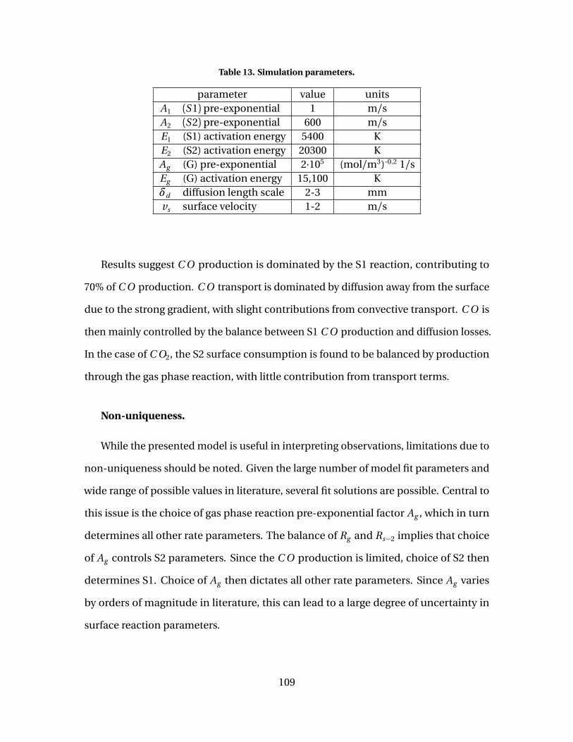
Table 13. Simulation parameters.
parameter value unitsA1 (S1) pre-exponential 1 m/sA2 (S2) pre-exponential 600 m/sE1 (S1) activation energy 5400 KE2 (S2) activation energy 20300 KAg (G) pre-exponential 2·105 (mol/m3)-0.2 1/sEg (G) activation energy 15,100 Kδd diffusion length scale 2-3 mmvs surface velocity 1-2 m/s
Results suggest C O production is dominated by the S1 reaction, contributing to
70% of C O production. C O transport is dominated by diffusion away from the surface
due to the strong gradient, with slight contributions from convective transport. C O is
then mainly controlled by the balance between S1 C O production and diffusion losses.
In the case of C O2, the S2 surface consumption is found to be balanced by production
through the gas phase reaction, with little contribution from transport terms.
Non-uniqueness.
While the presented model is useful in interpreting observations, limitations due to
non-uniqueness should be noted. Given the large number of model fit parameters and
wide range of possible values in literature, several fit solutions are possible. Central to
this issue is the choice of gas phase reaction pre-exponential factor Ag , which in turn
determines all other rate parameters. The balance of Rg and Rs−2 implies that choice
of Ag controls S2 parameters. Since the C O production is limited, choice of S2 then
determines S1. Choice of Ag then dictates all other rate parameters. Since Ag varies
by orders of magnitude in literature, this can lead to a large degree of uncertainty in
surface reaction parameters.
109
6.6 Conclusions
We presented the first spatially resolved graphite oxidation measurements in a flat
plate shear flow using IFTS. The oxidation of laser irradiated graphite in a reacting flow
has been observed for three graphite materials at irradiances of 750 and 1500 W/cm2
and freestream velocity of 5, 7, and 10 m/s. [C O ]/[C O2] data is presented for varying
material, irradiance, and freestream velocity with a general trend of [C O ]/[C O2] =
(7.8±1.3)exp(−3130±310/Ts ).
A simple model incorporating transport and kinetics is presented to interpret ex-
perimental observations. Increase in Ts results in an increase in C O due to increased
surface reactivity, increasing the diffusion length. Higher Ts also decreases C O2 due
to increasing consumption from the S2 reaction, as observed by the dip in C O2 near
laser center. Downstream of laser center, the loss in C O2 due to surface oxidation is
offset by the C O to C O2 conversion, resulting in an increase in C O2 profiles. Increasing
v∞ results in a decrease in δR , likely due to a decrease in boundary layer thickness.
The decrease in diffusion length leads to higher C O diffusion losses, decreasing C O
population. This results in a decrease in C O2 production in the gas phase, lowering the
C O2 population.
Relative strengths of kinetic and transport mechanisms are determined using a least
squares fit of species profiles along the surface. Results suggest that C O population is
determined by the balance between production at the surface, predominantly through
the S1 reaction, and diffusion losses. For C O2, transport terms are negligible, leading
to a balance between C O2 consumed at the surface through S2 and produced through
C O oxidation in the gas phase. Although general trends for C O and C O2 surface
profiles can be observed using the simplified model, it is difficult to perfectly replicate
experimental results, likely due to the overly simplified kinetic and transport models.
Full 2D simulations are necessary to gain a full picture of kinetic-transport coupling.
110

This highlights the necessity of CFD simulations which can not only greatly improve
transport modeling, but can also incorporate complex kinetic rate packages.
111
VII. Imaging Fourier Transform Spectroscopy of Graphite Oxidationin a Stagnation Flow
This chapter focuses on characterizing graphite oxidation in stagnation flow using
IFTS, in partial fulfillment of objective 1. The chapter is written in journal article format
and can be read independently as a stand alone document. Additional details regarding
background and experimental method can be found in Chapter II and IV, respectively.
7.1 Abstract
The oxidation of laser irradiated graphite in stagnation flow is characterized using
imaging Fourier transform spectroscopy (IFTS). Graphite cone samples were placed in
a 1.5 m/s dry (20% O2, < 1% H2O ) stagnation flow and irradiated at 650, 900, and 2400
W/cm2, producing surface temperatures of up to 3100 K. The resulting reacting layer
is observed using a midwave (MW) IFTS at 2 cm-1 spectral resolution, 0.5 mm/pixel
spatial resolution, and 0.75 Hz data cube rate. A cross-correlation technique for inferring
velocity maps from IFTS imagery is demonstrated. Plume temperature, C O , and C O2
concentrations are inferred from the IFTS spectral data. Temporal variations in the C O
and C O2 populations suggest some inhibition of the Cs −C O2 reaction with increasing
C O population. [C O ]/[C O2] trends at lower temperatures compare favorably with
previously reported values, with a general trend of: [C O ]/[C O2] = 2exp(−2400/Ts ). At
higher temperatures, these trends transition to higher effective activation energies of
16,000 and 31,000 K. This transition coincides with the decline in C O2 due to the Cs−C O2.
Additional data is needed to characterize the Cs −C O2 reaction and its dependence
on C O and Ts . This data set represents the first spatially resolved measurements of
graphite oxidation in a flat plate shear flow.
112

7.2 Introduction
Although carbon oxidation has been studied extensively, much is still not understood
regarding the coupling of kinetics and transport mechanisms. Carbon oxidation can be
simplified to the reactions shown in Table 14. The C O produced at the surface through
S1 and S2 is converted to C O2 as it diffuses away from the surface. A portion of the
C O2 then diffuses back to the surface to supply the S2 reaction. The C O oxidation in
the reacting layer then controls the oxidizing species available at the surface through
consumption of O2 and production of C O2. Accurately predicting carbon oxidation
then requires detailed knowledge of C O and surface oxidation mechanisms as well as
mass transport.
Table 14. Oxidation mechanisms
Reaction
(G) C O +1/2O2 =⇒ C O2
(S1) 2Cs +O2 =⇒ 2C O(S2) Cs +C O2 =⇒ 2C O
Imaging Fourier transform spectroscopy (IFTS) has recently been demonstrated
as a useful tool to characterize graphite oxidation in a reacting flow [1]. C O and C O2
spectral features in the midwave infrared (MWIR) were used to infer 2D maps of plume
temperature and species concentration. Combined with surface temperature measure-
ments using MWIR imagery, this technique allows full spatial characterization of the
oxidizing surface and reacting plume. These species maps provide unique insight into
how species are formed and transported from the surface. In the previous chapters, IFTS
was used to characterize graphite oxidation in buoyant flow and flat plate shear flow for
varying surface temperatures (Ts = 1000−4000 K) and graphite materials. Similar trends
113

in species population were observed for both flow cases. C O population was found
to be highly correlated with surface temperature as a result of the S1 and S2 surface
reactions. A decline in C O2 population was observed near laser center due to the S2
reaction.
Carbon oxidation studies are often presented in terms of [C O ]/[C O2] product ratio,
typically expressed as:[C O ][C O2]
=αexp�
−β
Ts
�
(141)
where α and β are found to vary significantly across literature due to differences in
material composition and test conditions (see Chapter II). In the case of buoyant
flow, little difference in [C O ]/[C O2]was seen across materials, with a general trend of
[C O ]/[C O2] = 22 · e x p (−6,000/Ts ). Similarly for flat plate shear flow, a general trend
of [C O ]/[C O2] = 8 · e x p (−3,100/Ts )was observed. These studies were conducted us-
ing identical materials over similar temperature ranges, suggesting that differences
in [C O ]/[C O2] trends are a result of variations in transport effects between the two
flow conditions. Although β values for buoyant and flat plate shear flow are within
the range typically observed in literature (β = 3,020 - 7,200 K) [21, 37–42], these de-
viate significantly from those reported by Acosta (β = 18,000 K) for similar surface
temperatures and material[1]. This variation in β values may be due differences in the
evaluation of [C O ]/[C O2]. In the Acosta study, product ratios were evaluated at a single
spatial point over the transient heating period, or ([C O ]/[C O2])(t ) vs Ts (t ). Whereas in
recent work, [C O ]/[C O2]was evaluated at steady state using the spatial distribution,
or ([C O ]/[C O2])(x ) vs Ts (x ). Ideally, this would be confirmed by comparison of the
transient response for both data sets. However the high heating rates for the more
recent data sets prevent characterization during the transient period.
The current study focuses on characterizing laser irradiated graphite in a stagnation
flow using IFTS. Graphite samples are irradiated in stagnation flow (v = 1.5 m/s) to
114

surface temperatures of up to 3100 K. Lower heating rates are used to allow for character-
ization of transient C O and C O2 populations. Differences in [C O ]/[C O2] concentration
ratios across the three flow conditions (buoyant flow, flat plate sheer flow, and stagnation
flow) are discussed. This data set represents the first spatially resolved measurements
of graphite oxidation in stagnation flow.
7.3 Experimental
Overview.
A schematic of the experimental set-up is shown in Figure 49. Samples were tested
at the Wright-Patterson Air Force Base Laser Hardened Materials Evaluation Laboratory
(LHMEL) using a 15 kW fiber laser at 1.07 µm, which produced a 1.3 cm diameter
beam, where beam area, Ab , is defined as containing 86% of laser power. Samples were
irradiated at 660 and 900 W /c m 2 until reaching surface temperatures of up to 2500 K.
Quoted irradiance values are spatially averaged over the beam profile (I = P o w e r /Ab ).
Stagnation flow was established using a 2.5 cm diameter nozzle, designed to produce
a flat top exit flow. A 1.5 m/s dry air (< 2% H2O ) flow was established over the 6 in
diameter cone test samples, creating a 3D stagnation flow with stagnation velocity
gradient, B = 3v∞/d = 30 s-1 (v∞ - flow velocity, d - sample diameter).
Graphite Samples .
Graphite samples were fine grade Graphtek GR008G samples which are produced
through an extrusion method. Material properties are outlined in Table 15 [3]. Impuri-
ties found in the ash content are not reported by the manufacturer, but previous work
report observations of Si, S, Fe, Ca, Al, and K [58]. Emissivities included are based on
measurements of post irradiated samples [82]. Samples were machined into an ogive
115
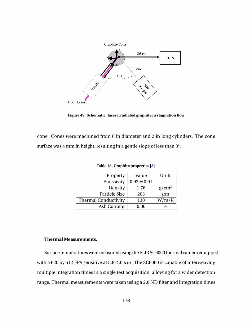
Figure 49. Schematic: laser irradiated graphite in stagnation flow
cone. Cones were machined from 6 in diameter and 2 in long cylinders. The cone
surface was 4 mm in height, resulting in a gentle slope of less than 3°.
Table 15. Graphite properties [3]
Property Value UnitsEmissivity 0.93 ± 0.01
Density 1.76 g/cm3
Particle Size 203 µmThermal Conductivity 130 W/m/K
Ash Content 0.06 %
Thermal Measurements.
Surface temperatures were measured using the FLIR SC6000 thermal camera equipped
with a 620 by 512 FPA sensitive at 3.8-4.0 µm . The SC6000 is capable of interweaving
multiple integration times in a single test acquisition, allowing for a wider detection
range. Thermal measurements were taken using a 2.0 ND filter and integration times
116

of 0.1-1.5 ms, resulting in a noise floor of 500 K. Images were were taken at 10 Hz and
window size of 128x160 to reduce data volume. The FLIR was mounted 51 degrees off
normal to avoid laser path, resulting in vertical and horizontal spatial resolutions of 0.8
and 1.2 mm/pixel respectively. Raw signal is converted to temperature measurements
using an external blackbody (320-870 K) and calibrating using the material emissivities
[82]. The largest source of error is the uncertainty in material emissivity, which can lead
to a temperature uncertainties of 3000±20 K.
Plume Measurements.
The reacting layer was observed along the z axis using the Telops MWIR hyperspec-
tral imager and Phantom v7 visible high speed camera. The MWIR Telops is an imaging
Fourier Transform spectrometer (IFTS) which provides spectral content at each pixel
in a 320 by 256 InSb focal plane array (FPA) responsive from 1800-6667 cm-1(λ = 1.5
- 5.5 µm) with a variable spectral resolution of ∆ν= 0.25 - 16 cm-1. A 2 cm-1 spectral
resolution was chosen to allow for adequate resolution of CO rotational features. A
reduced window size of 64 x 256 was chosen to increase data cube rate (0.75 cubes/s).
The 1.4 mrad pixel FOV resulted in a 0.5 mm/pixel spatial resolution. Further detail
regarding the MW Telops can be found in [61, 64, 79–81].
A simple two layer radiative transfer model (RTM) is used to fit the measured spectra.
The measured spectra can be expressed as:
Ld e t =τa t mo s · [εp l ume (n , X i−p l ume , Tp l ume ,`) ·B (Tp l ume ) +γB (Tp l ume )] (142)
where Ld e t is the measured spectral radiance, τa t mo s is the path transmission, εp l ume
is the plume spectral emissivity, and B (Ti ) is the spectral radiance of a blackbody at Ti .
The γB (ν, Tp l ume ) term was added to account for the background radiance due to soot
particles, which is assumed to be wavelength independent. Soot volume fraction is
117
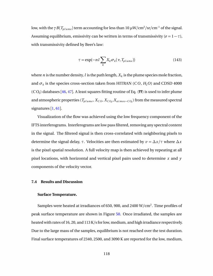
low, with the γB (Tp l ume ) term accounting for less than 10 µW/cm2/sr/cm-1 of the signal.
Assuming equilibrium, emissivity can be written in terms of transmissivity (ε = 1−τ),
with transmissivity defined by Beer’s law:
τ= exp(−nl∑
k
Xkσk (ν, Tp l ume )) (143)
where n is the number density, l is the path length, Xk is the plume species mole fraction,
and σk is the species cross-section taken from HITRAN (C O , H2O ) and CDSD 4000
(C O2) databases [46, 47]. A least squares fitting routine of Eq. (??) is used to infer plume
and atmospheric properties (Tp l ume , XC O , XC O2,Xa t mo s−C O2
) from the measured spectral
signatures [1, 61].
Visualization of the flow was achieved using the low frequency component of the
IFTS interferograms. Interferograms are low pass filtered, removing any spectral content
in the signal. The filtered signal is then cross-correlated with neighboring pixels to
determine the signal delay, τ. Velocities are then estimated by v = ∆x/τ where ∆x
is the pixel spatial resolution. A full velocity map is then achieved by repeating at all
pixel locations, with horizontal and vertical pixel pairs used to determine x and y
components of the velocity vector.
7.4 Results and Discussion
Surface Temperature.
Samples were heated at irradiances of 650, 900, and 2400 W/cm2. Time profiles of
peak surface temperature are shown in Figure 50. Once irradiated, the samples are
heated with rates of 16, 20, and 113 K/s for low, medium, and high irradiance respectively.
Due to the large mass of the samples, equilibrium is not reached over the test duration.
Final surface temperatures of 2340, 2500, and 3090 K are reported for the low, medium,
118
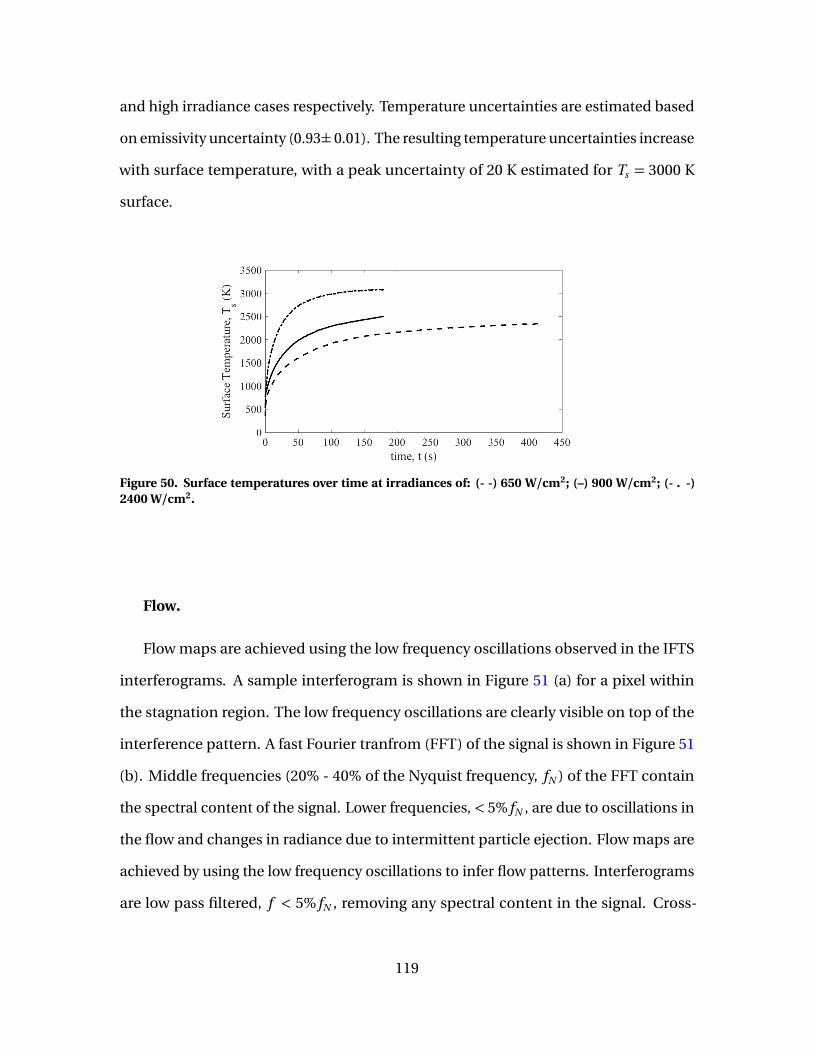
and high irradiance cases respectively. Temperature uncertainties are estimated based
on emissivity uncertainty (0.93± 0.01). The resulting temperature uncertainties increase
with surface temperature, with a peak uncertainty of 20 K estimated for Ts = 3000 K
surface.
Figure 50. Surface temperatures over time at irradiances of: (- -) 650 W/cm2; (–) 900 W/cm2; (- . -)2400 W/cm2.
Flow.
Flow maps are achieved using the low frequency oscillations observed in the IFTS
interferograms. A sample interferogram is shown in Figure 51 (a) for a pixel within
the stagnation region. The low frequency oscillations are clearly visible on top of the
interference pattern. A fast Fourier tranfrom (FFT) of the signal is shown in Figure 51
(b). Middle frequencies (20% - 40% of the Nyquist frequency, fN ) of the FFT contain
the spectral content of the signal. Lower frequencies, < 5% fN , are due to oscillations in
the flow and changes in radiance due to intermittent particle ejection. Flow maps are
achieved by using the low frequency oscillations to infer flow patterns. Interferograms
are low pass filtered, f < 5% fN , removing any spectral content in the signal. Cross-
119
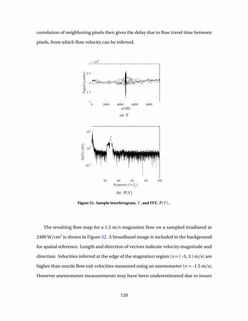
correlation of neighboring pixels then gives the delay due to flow travel time between
pixels, from which flow velocity can be inferred.
(a) Y
(b) F (Y )
Figure 51. Sample interferogram, Y , and FFT,F (Y ) .
The resulting flow map for a 1.5 m/s stagnation flow on a sampled irradiated at
2400 W/cm2 is shown in Figure 52. A broadband image is included in the background
for spatial reference. Length and direction of vectors indicate velocity magnitude and
direction. Velocities inferred at the edge of the stagnation region (v= ( -3, 3 ) m/s) are
higher than nozzle flow exit velocities measured using an anemometer (v = -1.5 m/s).
However anemometer measurements may have been underestimated due to issues
120

coupling the anemometer to the nozzle exit. Within the stagnation region, the flow
deviates from an ideal stagnation flow due to buoyancy effects, as evident by the upward
movement of the plume below centerline. A stagnation region is visible approximately
1 mm away from the surface. This is consistent with current modeling approach which
models graphite oxidation in stagnation flow as a counterflow problem [8]. In this case,
surface oxidation products are modeled as being ejected from the surface, creating a
stagnation plane as it interacts with the incoming flow.
121
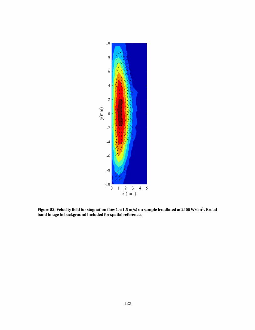
Figure 52. Velocity field for stagnation flow (v=1.5 m/s) on sample irradiated at 2400 W/cm2. Broad-band image in background included for spatial reference.
122
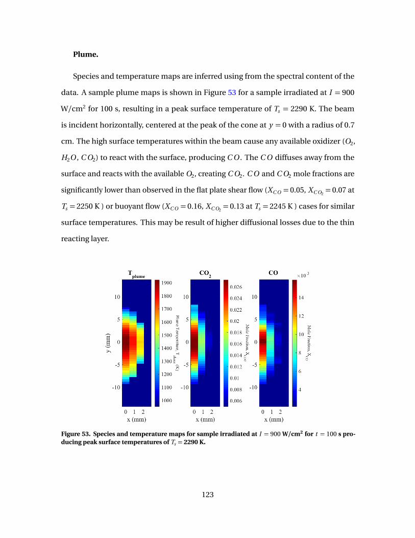
Plume.
Species and temperature maps are inferred using from the spectral content of the
data. A sample plume maps is shown in Figure 53 for a sample irradiated at I = 900
W/cm2 for 100 s, resulting in a peak surface temperature of Ts = 2290 K. The beam
is incident horizontally, centered at the peak of the cone at y = 0 with a radius of 0.7
cm. The high surface temperatures within the beam cause any available oxidizer (O2,
H2O , C O2) to react with the surface, producing C O . The C O diffuses away from the
surface and reacts with the available O2, creating C O2. C O and C O2 mole fractions are
significantly lower than observed in the flat plate shear flow (XC O = 0.05, XC O2= 0.07 at
Ts = 2250 K ) or buoyant flow (XC O = 0.16, XC O2= 0.13 at Ts = 2245 K ) cases for similar
surface temperatures. This may be result of higher diffusional losses due to the thin
reacting layer.
Figure 53. Species and temperature maps for sample irradiated at I = 900 W/cm2 for t = 100 s pro-ducing peak surface temperatures of Ts = 2290 K.
123
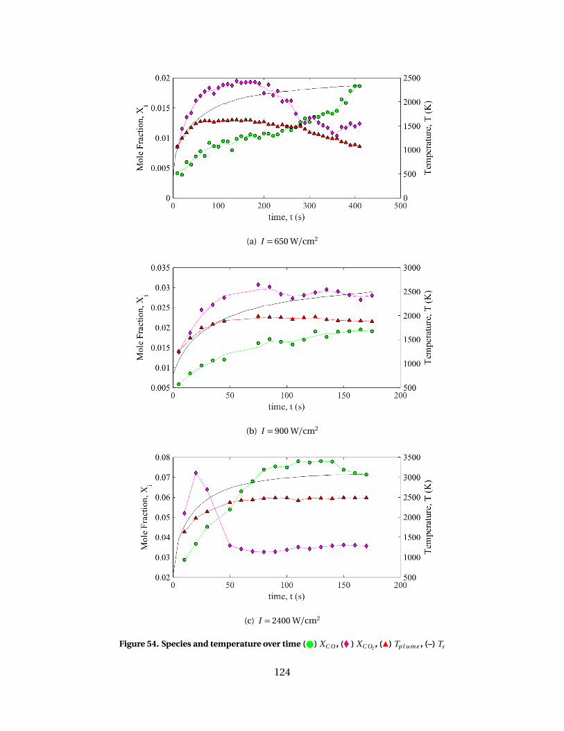
(a) I = 650 W/cm2
(b) I = 900 W/cm2
(c) I = 2400 W/cm2
Figure 54. Species and temperature over time ( ) XC O , (� ) XC O2, (Î) Tp l ume , (–) Ts
124

Evolving species concentrations and temperature are shown in Figure 54 for all
irradiance cases. In the initial heating stage, plume temperature is highly correlated
to surface temperature, followed by a leveling off at 1500, 2000 and 2500 K for the low,
medium, high irradiance cases respectively. Surface reactivity rises with Ts , resulting
in an increase in C O over time for all cases. The most notable difference between the
three cases is the C O2 time profile. In the low irradiance case, C O2 initially rises with
temperature, but then declines significantly at Ts > 2150 K. The drop in C O2 coincides
with a cooling in plume temperature, and slight increase in C O growth rate. This
suggests these observations are a result of the endothermic S2 reaction which converts
C O2 to C O . A similar trend is observed in the high irradiance case, with C O2 dropping
after Ts > X K. However, these trends are not observed in the medium irradiance case.
One possible explanation of this is inhibition of the S2 reaction by C O [85], which may
influencing the reactivity of S2.
[C O ]/[C O2] Temperature Dependence.
Plots of [C O ]/[C O2] versus inverse surface temperature are given in Figure 55. At
lower temperatures, all test cases follow the general trend of:
[C O ][C O2]
= 1.7±0.3 ·exp�−2400±400
T
�
(144)
β values are consistent with those reported fro the flat plate shear flow cases (β = 2700
K) and in reasonable agreement with values reported by Tognotti, Otterbien, Phillips,
Du, and Walker (β = 3000−3200 K) [21, 39–41, 89].
At higher temperatures where the decline in C O2 is observed, the slope changes
dramatically. The high and low irradiance cases can then be characterized β values
of 16,000 and 31,000 K respectively. While these results are significantly higher than
flat plate case, they are comparable to those reported by Acosta (β = 18, 000 K) [7]. The
125
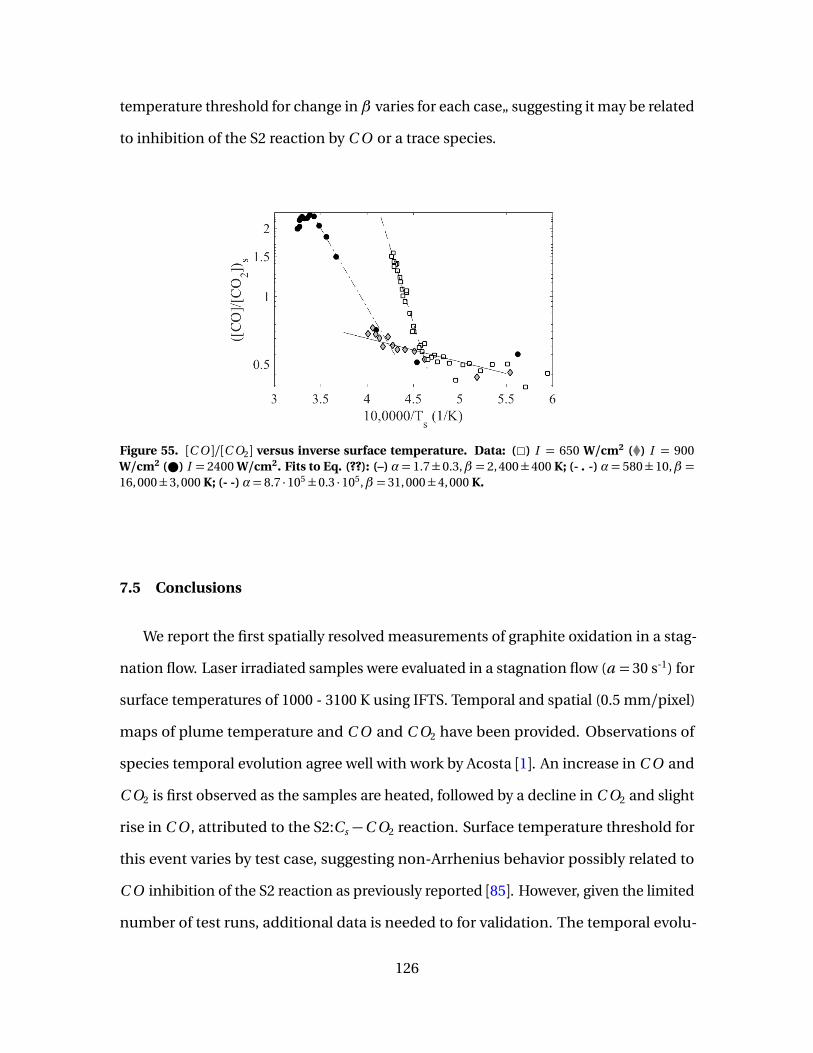
temperature threshold for change in β varies for each case„ suggesting it may be related
to inhibition of the S2 reaction by C O or a trace species.
Figure 55. [C O ]/[C O2] versus inverse surface temperature. Data: (2) I = 650 W/cm2 (�) I = 900W/cm2 ( ) I = 2400 W/cm2. Fits to Eq. (??): (–) α= 1.7±0.3,β = 2,400±400 K; (- . -) α= 580±10,β =16, 000±3, 000 K; (- -) α= 8.7 ·105±0.3 ·105,β = 31, 000±4, 000 K.
7.5 Conclusions
We report the first spatially resolved measurements of graphite oxidation in a stag-
nation flow. Laser irradiated samples were evaluated in a stagnation flow (a = 30 s-1) for
surface temperatures of 1000 - 3100 K using IFTS. Temporal and spatial (0.5 mm/pixel)
maps of plume temperature and C O and C O2 have been provided. Observations of
species temporal evolution agree well with work by Acosta [1]. An increase in C O and
C O2 is first observed as the samples are heated, followed by a decline in C O2 and slight
rise in C O , attributed to the S2:Cs −C O2 reaction. Surface temperature threshold for
this event varies by test case, suggesting non-Arrhenius behavior possibly related to
C O inhibition of the S2 reaction as previously reported [85]. However, given the limited
number of test runs, additional data is needed to for validation. The temporal evolu-
126
tion of [C O ]/[C O2] concentration ratios is evaluated at laser center. Results show two
general trends. At lower temperatures, trends of [C O ]/[C O2] = 1.7exp(−2400/T ) are
observed. This is general agreement with steady state observations for flat plate shear
flow (β = 3100 K). When the C O2 population declines at higher temperatures (2200-
2500 K), β values increase significantly, with trends of β = 16,000 and 31,000 K. Higher
β values are consistent with transient observations reported by Acosta (β = 18,000 K)[1],
but it is unclear what produces these differences in β values.
This work provides the first demonstration of flow velocimetry using IFTS. Corre-
lation of low frequency oscillations in raw IFTS data allow for identification of flow
patterns. Magnitudes of the flow velocities can then be roughly estimated using camera
frame rates, pixel resolution, and the delay inferred from cross-correlation. Flow maps
show deviation from ideal stagnation flow due to buoyancy effects. However results
suggest a counterflow like pattern between surface oxidation products being ejected
from the surface and the incoming stagnation flow, with a stagnation zone visible 1 mm
away from the surface.
127
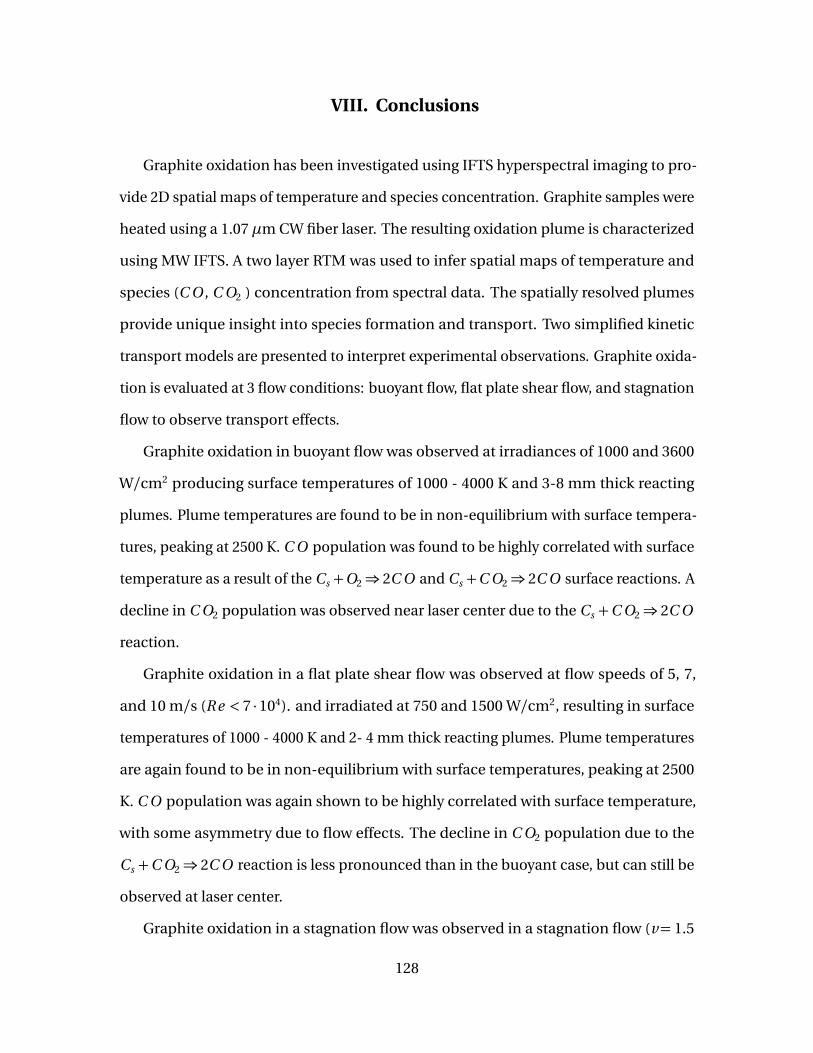
VIII. Conclusions
Graphite oxidation has been investigated using IFTS hyperspectral imaging to pro-
vide 2D spatial maps of temperature and species concentration. Graphite samples were
heated using a 1.07 µm CW fiber laser. The resulting oxidation plume is characterized
using MW IFTS. A two layer RTM was used to infer spatial maps of temperature and
species (C O , C O2 ) concentration from spectral data. The spatially resolved plumes
provide unique insight into species formation and transport. Two simplified kinetic
transport models are presented to interpret experimental observations. Graphite oxida-
tion is evaluated at 3 flow conditions: buoyant flow, flat plate shear flow, and stagnation
flow to observe transport effects.
Graphite oxidation in buoyant flow was observed at irradiances of 1000 and 3600
W/cm2 producing surface temperatures of 1000 - 4000 K and 3-8 mm thick reacting
plumes. Plume temperatures are found to be in non-equilibrium with surface tempera-
tures, peaking at 2500 K. C O population was found to be highly correlated with surface
temperature as a result of the Cs +O2⇒ 2C O and Cs +C O2⇒ 2C O surface reactions. A
decline in C O2 population was observed near laser center due to the Cs +C O2⇒ 2C O
reaction.
Graphite oxidation in a flat plate shear flow was observed at flow speeds of 5, 7,
and 10 m/s (R e < 7 ·104). and irradiated at 750 and 1500 W/cm2, resulting in surface
temperatures of 1000 - 4000 K and 2- 4 mm thick reacting plumes. Plume temperatures
are again found to be in non-equilibrium with surface temperatures, peaking at 2500
K. C O population was again shown to be highly correlated with surface temperature,
with some asymmetry due to flow effects. The decline in C O2 population due to the
Cs +C O2⇒ 2C O reaction is less pronounced than in the buoyant case, but can still be
observed at laser center.
Graphite oxidation in a stagnation flow was observed in a stagnation flow (v= 1.5
128
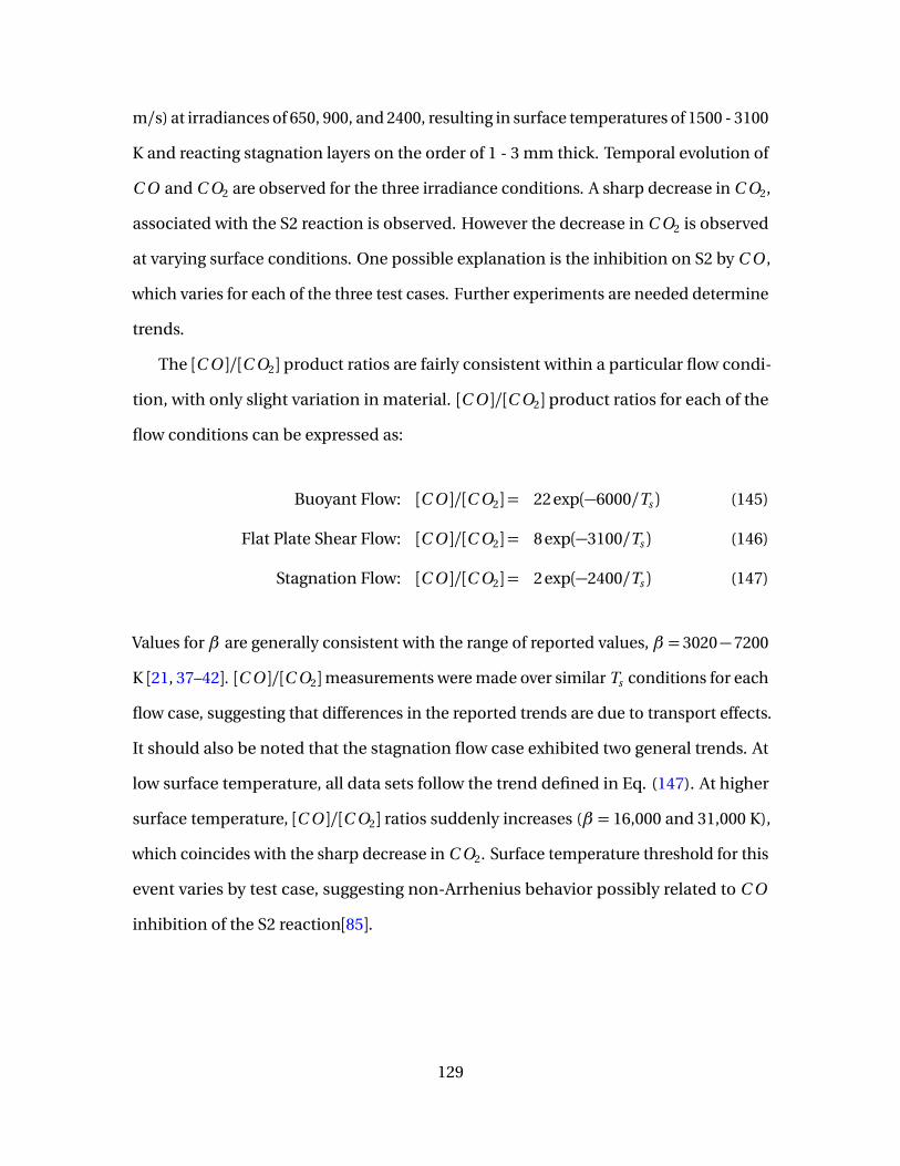
m/s) at irradiances of 650, 900, and 2400, resulting in surface temperatures of 1500 - 3100
K and reacting stagnation layers on the order of 1 - 3 mm thick. Temporal evolution of
C O and C O2 are observed for the three irradiance conditions. A sharp decrease in C O2,
associated with the S2 reaction is observed. However the decrease in C O2 is observed
at varying surface conditions. One possible explanation is the inhibition on S2 by C O ,
which varies for each of the three test cases. Further experiments are needed determine
trends.
The [C O ]/[C O2] product ratios are fairly consistent within a particular flow condi-
tion, with only slight variation in material. [C O ]/[C O2] product ratios for each of the
flow conditions can be expressed as:
Buoyant Flow: [C O ]/[C O2] = 22 exp(−6000/Ts ) (145)
Flat Plate Shear Flow: [C O ]/[C O2] = 8 exp(−3100/Ts ) (146)
Stagnation Flow: [C O ]/[C O2] = 2 exp(−2400/Ts ) (147)
Values for β are generally consistent with the range of reported values, β = 3020−7200
K [21, 37–42]. [C O ]/[C O2]measurements were made over similar Ts conditions for each
flow case, suggesting that differences in the reported trends are due to transport effects.
It should also be noted that the stagnation flow case exhibited two general trends. At
low surface temperature, all data sets follow the trend defined in Eq. (147). At higher
surface temperature, [C O ]/[C O2] ratios suddenly increases (β = 16,000 and 31,000 K),
which coincides with the sharp decrease in C O2. Surface temperature threshold for this
event varies by test case, suggesting non-Arrhenius behavior possibly related to C O
inhibition of the S2 reaction[85].
129
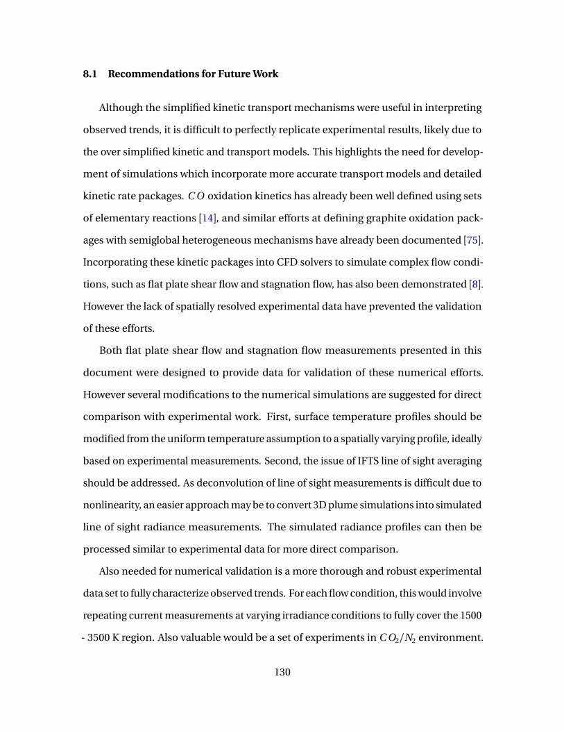
8.1 Recommendations for Future Work
Although the simplified kinetic transport mechanisms were useful in interpreting
observed trends, it is difficult to perfectly replicate experimental results, likely due to
the over simplified kinetic and transport models. This highlights the need for develop-
ment of simulations which incorporate more accurate transport models and detailed
kinetic rate packages. C O oxidation kinetics has already been well defined using sets
of elementary reactions [14], and similar efforts at defining graphite oxidation pack-
ages with semiglobal heterogeneous mechanisms have already been documented [75].
Incorporating these kinetic packages into CFD solvers to simulate complex flow condi-
tions, such as flat plate shear flow and stagnation flow, has also been demonstrated [8].
However the lack of spatially resolved experimental data have prevented the validation
of these efforts.
Both flat plate shear flow and stagnation flow measurements presented in this
document were designed to provide data for validation of these numerical efforts.
However several modifications to the numerical simulations are suggested for direct
comparison with experimental work. First, surface temperature profiles should be
modified from the uniform temperature assumption to a spatially varying profile, ideally
based on experimental measurements. Second, the issue of IFTS line of sight averaging
should be addressed. As deconvolution of line of sight measurements is difficult due to
nonlinearity, an easier approach may be to convert 3D plume simulations into simulated
line of sight radiance measurements. The simulated radiance profiles can then be
processed similar to experimental data for more direct comparison.
Also needed for numerical validation is a more thorough and robust experimental
data set to fully characterize observed trends. For each flow condition, this would involve
repeating current measurements at varying irradiance conditions to fully cover the 1500
- 3500 K region. Also valuable would be a set of experiments in C O2/N2 environment.
130

The removal of O2 from the environment provides two advantages. First, it would
allow isolation of the Cs − C O2 mechanism from any Cs −O2 interactions, allowing
for better observation of the S2 mechanism, particularly the inhibition due to C O .
Second, the removal of O2 would prevent the oxidation of C O after if it produced at the
surface, removing the complication of coupling of the heterogeneous and homogeneous
kinetics.
While IFTS has proven valuable for characterization of graphite oxidation, line of
sight averaging continues to be an issue when interpreting species and temperature
maps. This can be alleviated with the implementation of the multi-layer RTM method
[62]. Current measurements assume a uniform flame along the line of sight, which may
introduce systematic errors of up to 6% for plume temperature and 21% for species mole
fraction (see Appendix B). Recently a technique has been developed which leverages
the multiple line of sight measurements provided by IFTS to infer radial flame profiles
[62]. However implementation of this technique would require redesign of experiments
to produce a radially symmetric flame. This could be achieved through stagnation flow
measurements or by reorienting the buoyant flow measurements such that the sample
is prone with a upward buoyant symmetric flame.
Future laser lethality work will focus on more realistic materials, such as carbon
fiber. Much of the kinetics of carbon fiber oxidation is initially dominated by volatile
decomposition and combustion. However, once these volatiles are removed, the ma-
terial consists primarily of bare carbon fibers. Therefore simulations for bare carbon
fiber oxidation can build upon the heterogeneous rate packages developed for graphite
oxidation. A similar set of experimental data focusing on laser irradiated bare carbon
fibers would be required for validation.
131
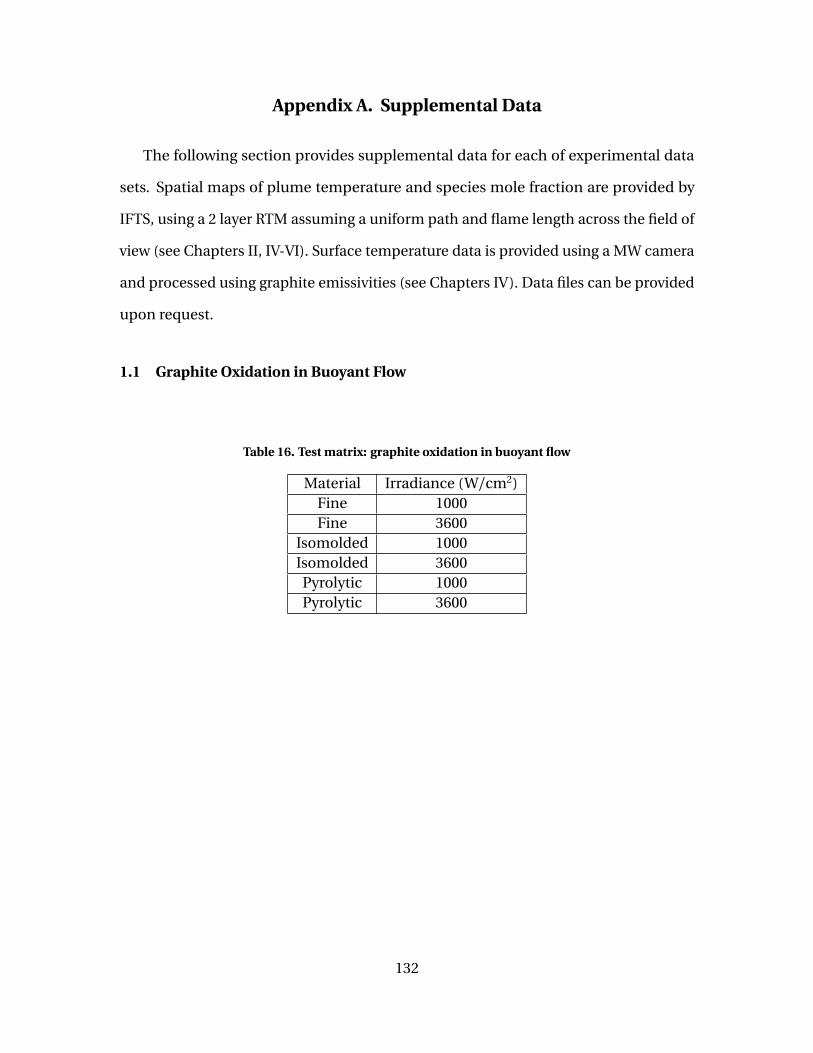
Appendix A. Supplemental Data
The following section provides supplemental data for each of experimental data
sets. Spatial maps of plume temperature and species mole fraction are provided by
IFTS, using a 2 layer RTM assuming a uniform path and flame length across the field of
view (see Chapters II, IV-VI). Surface temperature data is provided using a MW camera
and processed using graphite emissivities (see Chapters IV). Data files can be provided
upon request.
1.1 Graphite Oxidation in Buoyant Flow
Table 16. Test matrix: graphite oxidation in buoyant flow
Material Irradiance (W/cm2)Fine 1000Fine 3600
Isomolded 1000Isomolded 3600Pyrolytic 1000Pyrolytic 3600
132
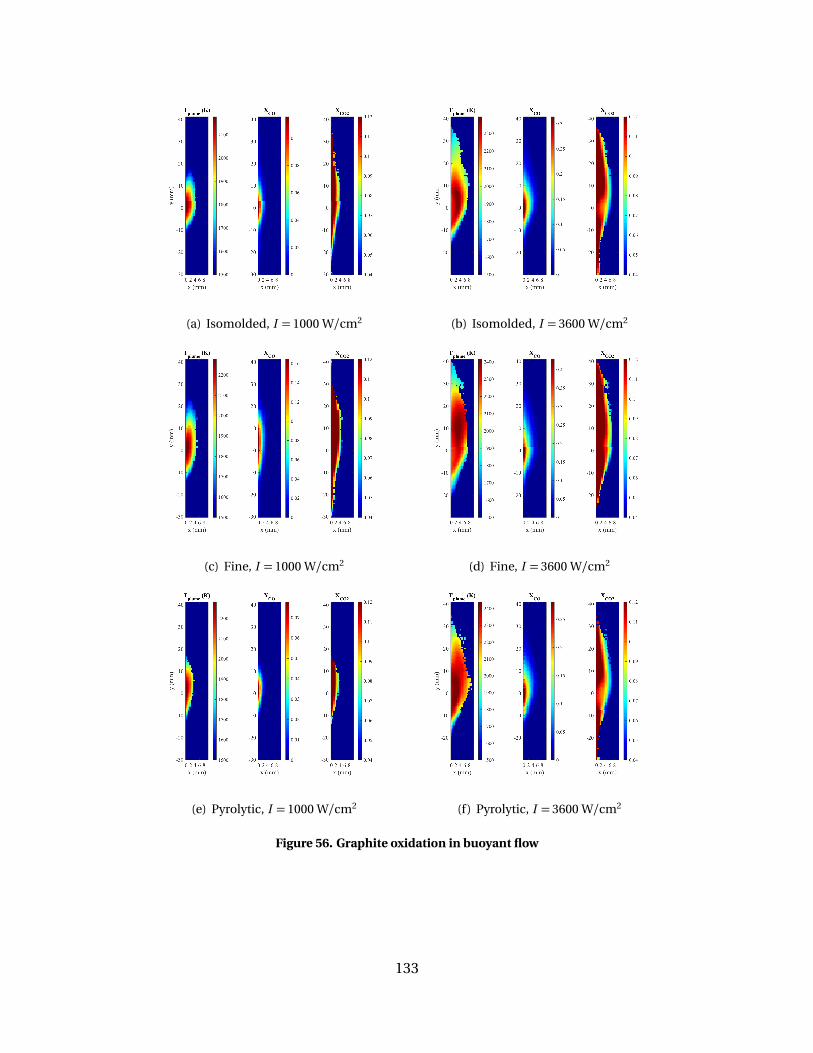
(a) Isomolded, I = 1000 W/cm2 (b) Isomolded, I = 3600 W/cm2
(c) Fine, I = 1000 W/cm2 (d) Fine, I = 3600 W/cm2
(e) Pyrolytic, I = 1000 W/cm2 (f) Pyrolytic, I = 3600 W/cm2
Figure 56. Graphite oxidation in buoyant flow
133

1.2 Graphite Oxidation in Flat Plate Shear Flow
Table 17. Test matrix: graphite oxidation in flat plate shear flow
Material Flow (m/s) Irradiance (W/cm2) NotesFine 5 750Fine 7 750Fine 10 750 no dataFine 5 1500Fine 7 1500Fine 10 1500
Isomolded 5 750Isomolded 7 750 no dataIsomolded 10 750Isomolded 5 1500Isomolded 7 1500Isomolded 10 1500Pyrolytic 5 750Pyrolytic 7 750Pyrolytic 10 750Pyrolytic 5 1500Pyrolytic 7 1500Pyrolytic 10 1500
134
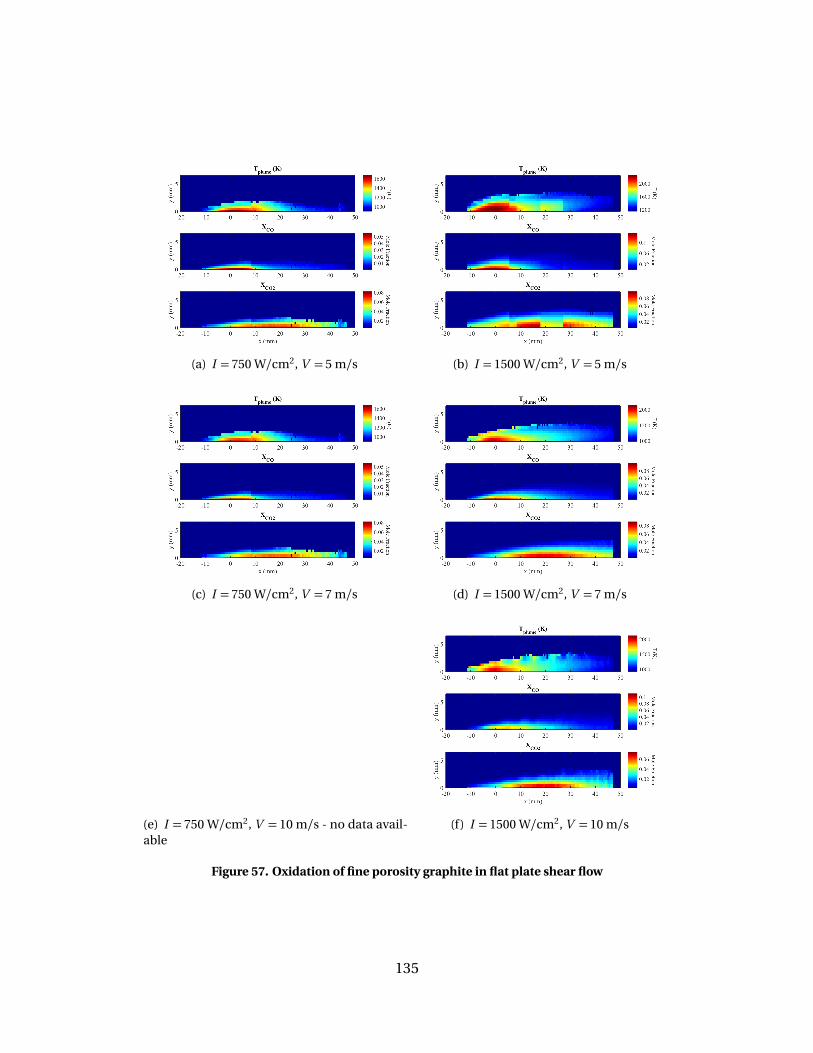
(a) I = 750 W/cm2, V = 5 m/s (b) I = 1500 W/cm2, V = 5 m/s
(c) I = 750 W/cm2, V = 7 m/s (d) I = 1500 W/cm2, V = 7 m/s
(e) I = 750 W/cm2, V = 10 m/s - no data avail-able
(f) I = 1500 W/cm2, V = 10 m/s
Figure 57. Oxidation of fine porosity graphite in flat plate shear flow
135
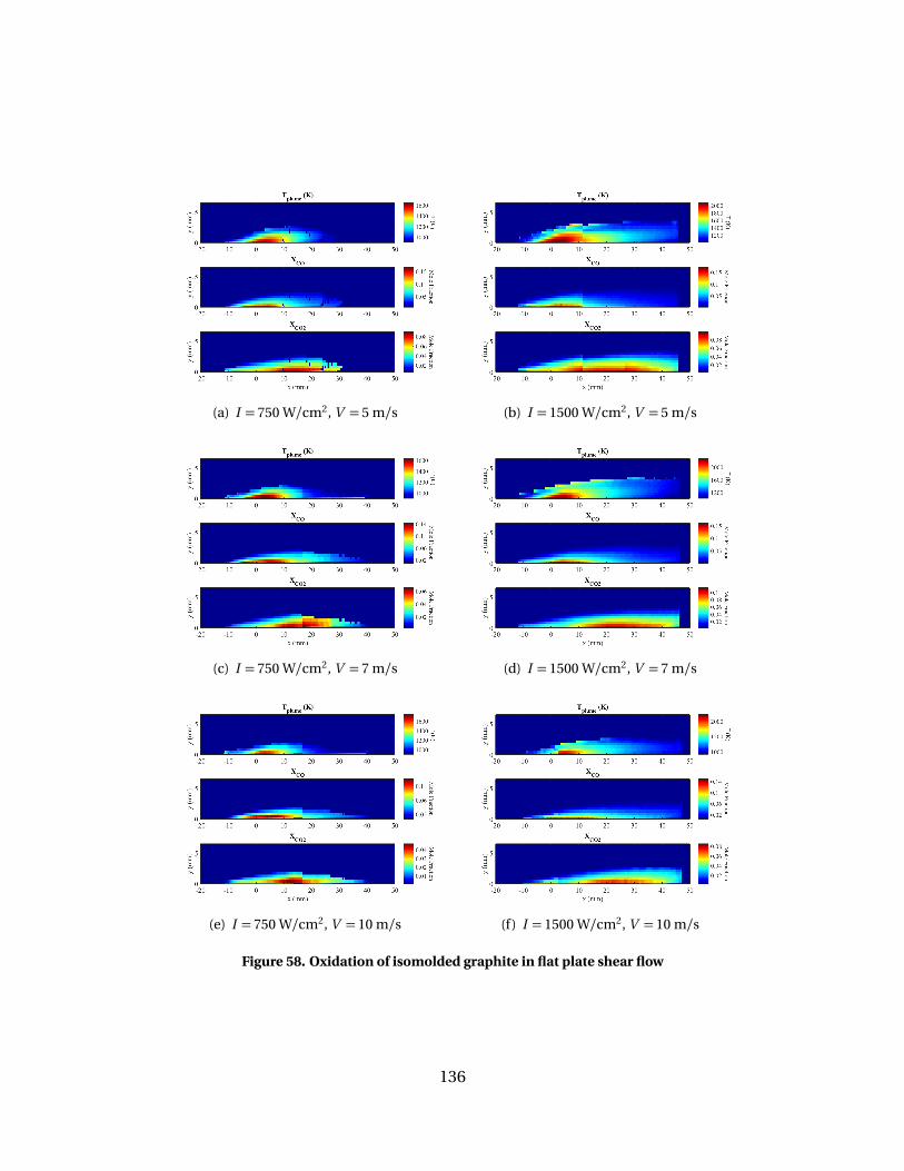
(a) I = 750 W/cm2, V = 5 m/s (b) I = 1500 W/cm2, V = 5 m/s
(c) I = 750 W/cm2, V = 7 m/s (d) I = 1500 W/cm2, V = 7 m/s
(e) I = 750 W/cm2, V = 10 m/s (f) I = 1500 W/cm2, V = 10 m/s
Figure 58. Oxidation of isomolded graphite in flat plate shear flow
136
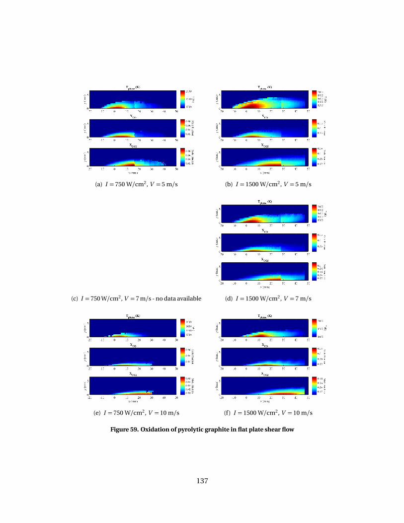
(a) I = 750 W/cm2, V = 5 m/s (b) I = 1500 W/cm2, V = 5 m/s
(c) I = 750 W/cm2, V = 7 m/s - no data available (d) I = 1500 W/cm2, V = 7 m/s
(e) I = 750 W/cm2, V = 10 m/s (f) I = 1500 W/cm2, V = 10 m/s
Figure 59. Oxidation of pyrolytic graphite in flat plate shear flow
137
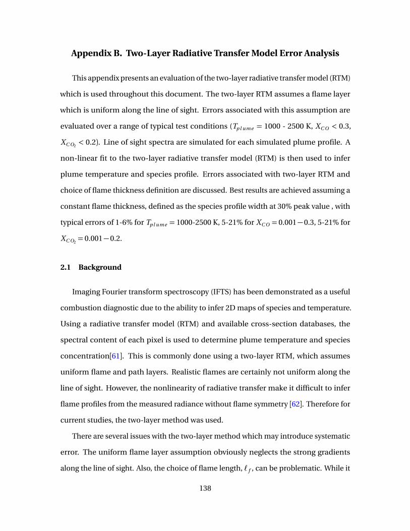
Appendix B. Two-Layer Radiative Transfer Model Error Analysis
This appendix presents an evaluation of the two-layer radiative transfer model (RTM)
which is used throughout this document. The two-layer RTM assumes a flame layer
which is uniform along the line of sight. Errors associated with this assumption are
evaluated over a range of typical test conditions (Tp l ume = 1000 - 2500 K, XC O < 0.3,
XC O2< 0.2). Line of sight spectra are simulated for each simulated plume profile. A
non-linear fit to the two-layer radiative transfer model (RTM) is then used to infer
plume temperature and species profile. Errors associated with two-layer RTM and
choice of flame thickness definition are discussed. Best results are achieved assuming a
constant flame thickness, defined as the species profile width at 30% peak value , with
typical errors of 1-6% for Tp l ume = 1000-2500 K, 5-21% for XC O = 0.001−0.3, 5-21% for
XC O2= 0.001−0.2.
2.1 Background
Imaging Fourier transform spectroscopy (IFTS) has been demonstrated as a useful
combustion diagnostic due to the ability to infer 2D maps of species and temperature.
Using a radiative transfer model (RTM) and available cross-section databases, the
spectral content of each pixel is used to determine plume temperature and species
concentration[61]. This is commonly done using a two-layer RTM, which assumes
uniform flame and path layers. Realistic flames are certainly not uniform along the
line of sight. However, the nonlinearity of radiative transfer make it difficult to infer
flame profiles from the measured radiance without flame symmetry [62]. Therefore for
current studies, the two-layer method was used.
There are several issues with the two-layer method which may introduce systematic
error. The uniform flame layer assumption obviously neglects the strong gradients
along the line of sight. Also, the choice of flame length, ` f , can be problematic. While it
138
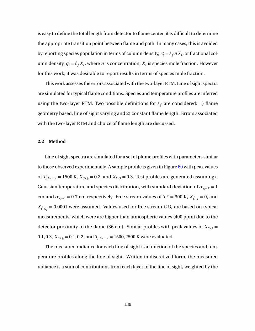
is easy to define the total length from detector to flame center, it is difficult to determine
the appropriate transition point between flame and path. In many cases, this is avoided
by reporting species population in terms of column density, c ′i = ` f n X i , or fractional col-
umn density, qi = ` f X i , where n is concentration, X i is species mole fraction. However
for this work, it was desirable to report results in terms of species mole fraction.
This work assesses the errors associated with the two-layer RTM. Line of sight spectra
are simulated for typical flame conditions. Species and temperature profiles are inferred
using the two-layer RTM. Two possible definitions for ` f are considered: 1) flame
geometry based, line of sight varying and 2) constant flame length. Errors associated
with the two-layer RTM and choice of flame length are discussed.
2.2 Method
Line of sight spectra are simulated for a set of plume profiles with parameters similar
to those observed experimentally. A sample profile is given in Figure 60 with peak values
of Tp l ume = 1500 K, XC O2= 0.2, and XC O = 0.3. Test profiles are generated assuming a
Gaussian temperature and species distribution, with standard deviation of σg−T = 1
cm and σg−c = 0.7 cm respectively. Free stream values of T o = 300 K, X oC O = 0, and
X oC O2= 0.0001 were assumed. Values used for free stream C O2 are based on typical
measurements, which were are higher than atmospheric values (400 ppm) due to the
detector proximity to the flame (36 cm). Similar profiles with peak values of XC O =
0.1, 0.3, XC O2= 0.1, 0.2, and Tp l ume = 1500, 2500 K were evaluated.
The measured radiance for each line of sight is a function of the species and tem-
perature profiles along the line of sight. Written in discretized form, the measured
radiance is a sum of contributions from each layer in the line of sight, weighted by the
139
Figure 60. Simulated Gaussian flame profile. Temperature: σg−T = 1 cm with peak value of Tp l ume =1500 K. Species: σg−c = 0.7 cm with peak values of XC O2
= 0.2 and XC O = 0.3.
transmissivity of subsequent layers:
L =K∑
i=1
εi (αi )B (Ti )K∏
j=i+1
τ j (α j )
!
(148)
where εi is the emissivity of layer i , B (Ti ) is the radiance of blackbody at temperature
Ti , and τ j is the transmissivity of of layer j . Assuming equilibrium, emissivity can be
written in terms of transmissivity, ε = 1−τ, where transmissivity is defined by Beer’s
Law in terms of optical depth, α:
τi = e x p (−αi ) (149)
αi = n`i
∑
m
Xmσm (ν, T ) (150)
where n is number density, `i is length of layer i , Xm is the mole fraction of species m ,
andσm is the cross-section of species m provided by HITRAN and CDSD databases.
Line of sight spectra are simulated using Eq. (148) at intervals of 0.05 cm based
on instrument resolution. A total distance of 36 cm from detector to flame center is
used based on current measurement conditions. A sample set of line of sight spectra is
shown in Figure 61 for peak values of Tp l ume = 1500K , C O = 0.1, and C O2 = 0.2. Differ-
140
ences in path transmissivity along different lines of sight is most visible in comparing
measurements at flame center (red) to outer layers, particularly in the 2300 - 2400 cm-1
C O2 feature.
Figure 61. Line of sight spectra generated using Eq. (148) for peak Tp l ume , C O , and C O2 of 1500 K,0.1 and 0.2 respectively. Color corresponds to line of sight location with red corresponding to flamecenter with LOS spacing of∆x = 0.05c m .
A two-layer radiative transfer model, similar to that used for experimental work, is
then fit to the simulated line of sight spectra to evaluate the use of the two-layer model.
The measured radiance can be expressed as:
Ld e t =τa t mo s (αa t mo s ) · εp l ume (αp l ume ) ·B (Tp l ume ) (151)
where αp l ume and αa t mo s are defined by Eq. (150) and plume and atmospheric parame-
ters. A non-linear least squares fitting routine is then used to solve for Tp l ume , Ta t mo s ,
qi−a t mo s , and qi−p l ume ) ,where qi is the fractional column density, qi = ` f X i .
Determination of species mole fraction then relies on choice of flame length, ` f .
141
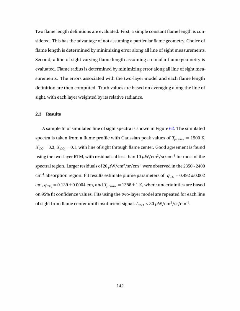
Two flame length definitions are evaluated. First, a simple constant flame length is con-
sidered. This has the advantage of not assuming a particular flame geometry. Choice of
flame length is determined by minimizing error along all line of sight measurements.
Second, a line of sight varying flame length assuming a circular flame geometry is
evaluated. Flame radius is determined by minimizing error along all line of sight mea-
surements. The errors associated with the two-layer model and each flame length
definition are then computed. Truth values are based on averaging along the line of
sight, with each layer weighted by its relative radiance.
2.3 Results
A sample fit of simulated line of sight spectra is shown in Figure 62. The simulated
spectra is taken from a flame profile with Gaussian peak values of Tp l ume = 1500 K,
XC O = 0.3, XC O2= 0.1, with line of sight through flame center. Good agreement is found
using the two-layer RTM, with residuals of less than 10 µW/cm2/sr/cm-1 for most of the
spectral region. Larger residuals of 20µW/cm2/sr/cm-1 were observed in the 2350 - 2400
cm-1 absorption region. Fit results estimate plume parameters of: qC O = 0.492±0.002
cm, qC O2= 0.139±0.0004 cm, and Tp l ume = 1388±1 K, where uncertainties are based
on 95% fit confidence values. Fits using the two-layer model are repeated for each line
of sight from flame center until insufficient signal, Ld e t < 30 µW/cm2/sr/cm-1.
142
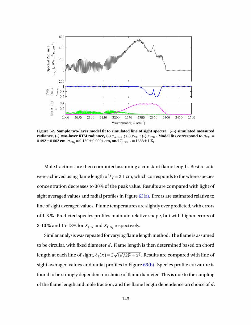
Figure 62. Sample two-layer model fit to simulated line of sight spectra. (-·-) simulated measuredradiance, (–) two-layer RTM radiance, (–) τa t mo s ; (–) εC O ; (–) εC O 2. Model fits correspond to qC O =0.492±0.002 cm, qC O2
= 0.139±0.0004 cm, and Tp l ume = 1388±1 K,
Mole fractions are then computed assuming a constant flame length. Best results
were achieved using flame length of ` f = 2.1 cm, which corresponds to the where species
concentration decreases to 30% of the peak value. Results are compared with light of
sight averaged values and radial profiles in Figure 63(a). Errors are estimated relative to
line of sight averaged values. Plume temperatures are slightly over predicted, with errors
of 1-3 %. Predicted species profiles maintain relative shape, but with higher errors of
2-10 % and 15-18% for XC O and XC O2respectively.
Similar analysis was repeated for varying flame length method. The flame is assumed
to be circular, with fixed diameter d . Flame length is then determined based on chord
length at each line of sight, ` f (x ) = 2p
(d /2)2+ x 2. Results are compared with line of
sight averaged values and radial profiles in Figure 63(b). Species profile curvature is
found to be strongly dependent on choice of flame diameter. This is due to the coupling
of the flame length and mole fraction, and the flame length dependence on choice of d .
143
Predicted species profiles show smaller errors than the constant flame length method,
with inner flame errors of <10 % for XC O and XC O2at x < 1 cm. However, species profile
curvature is poorly reconstructed. Results are even flatter for poor choice of flame
diameter.
Comparing the two methods, constant flame length is preferred due to better re-
construction of the species profile. In the case of constant flame length, poor choice
of ` f will only scale mole fraction profiles, but leave the relative shape intact. In the
case of variable flame length, poor choice of flame diameter can lead to large errors in
profile shape and relative value. The remaining test profiles were analyzed assuming a
constant flame length of 2.1 cm. Similar errors in plume temperature were reported
were reported across all cases, with errors of <6 %. Errors in species mole fraction of
5-21% were observed for XC O = 0.001−0.3 and XC O2= 0.001−0.2.
144
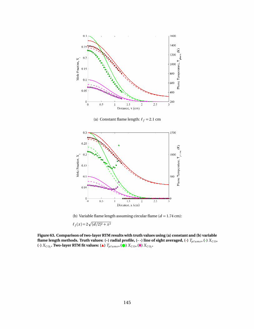
(a) Constant flame length: ` f = 2.1 cm
(b) Variable flame length assuming circular flame (d = 1.74 cm):
` f (x ) = 2p
(d /2)2+ x 2
Figure 63. Comparison of two-layer RTM results with truth values using (a) constant and (b) variableflame length methods. Truth values: (–) radial profile, (- -) line of sight averaged, (-) Tp l ume , (-) XC O ,(-) XC O2
. Two-layer RTM fit values: (Î) Tp l ume , ( ) XC O , (�) XC O2.
145
2.4 Summary
The two-layer RTM has been evaluated using simulated line of sight spectra for a
range of test profiles. Profiles were chosen to cover the range of typical test conditions,
with peak profile values of of XC O = 0.1,0.3, XC O2= 0.1,0.2, and Tp l ume = 1500,2500 K .
Two methods at defining flame length are evaluated: constant flame length, and variable
flame length based on flame geometry. Constant flame length is found to be preferable,
due to better reconstruction of the species profile curvature and less sensitivity to poor
choice in flame length. Results suggest errors for the two-layer method with constant
flame length may be as high as 21% for XC O and XC O2and 6% for Tp l ume . These errors
are significantly higher than those errors based on fit confidence levels, and highlight
the need for analysis of systematic errors when implementing the two-layer model.
146
Bibliography
1. Roberto I. Acosta, Kevin C. Gross, and Glen P. Perram. Combustion kinetics oflaser irradiated porous graphite from imaging Fourier transform spectroscopy.Combustion and Flame, 163:90–99, jan 2016.
2. G.W Autio and E Scala. The normal spectral emissivity of isotropic and anisotropicmaterials. Carbon, 4(1):13–28, may 1966.
3. GraphiteStore. https://www.graphitestore.com/, 2015.
4. Glen P Perram, Michael A Marciniak, and Matthew Goda. Laser Technologies forDefense and Security; High-energy laser weapons: technology overview. volume5414, page 1 <last_page> 25, 2004.
5. Annemie Bogaerts, Zhaoyang Chen, Renaat Gijbels, and Akos Vertes. Laser ablationfor analytical sampling: What can we learn from modeling? Spectrochimica Acta -Part B Atomic Spectroscopy, 58(11):1867–1893, 2003.
6. H. K. Chelliah. The influence of heterogeneous kinetics and thermal radiation onthe oxidation of graphite particles. Combustion and Flame, 104(1-2):81–94, 1996.
7. Roberto I Acosta. Imaging Fourier Transform Spectroscopy of the Boundary LayerPlume from Laser Irradiated Polymers and Carbon Materials. PhD thesis, AFIT, 2014.
8. Ryan Frederick Johnson. Multidimensional Reacting Flow Simulations with CoupledHomogeneous and Heterogeneous Models. PhD thesis, University of Virginia, 2014.
9. Christopher R. Shaddix, Franz Holzleithner, Manfred Geier, and Brian S. Haynes. Nu-merical assessment of Tognotti determination of CO2/CO production ratio duringchar oxidation. Combustion and Flame, 160(9):1827–1834, sep 2013.
10. Normand M Laurendeau. Heterogeneous kinetics of coal char gasification andcombustion. Progress in Energy and Combustion Science, 4(4):221 – 270, 1978.
11. a. Makino, N. Araki, and Y. Mihara. Combustion of artificial graphite in stagnationflow: Estimation of global kinetic parameters from experimental results. Combus-tion and Flame, 96(3):261–274, 1994.
12. Sang-min Lee, Dong-su Kang, and Jea-seung Roh. Bulk graphite : materials andmanufacturing process. Carbon Letters, 16(3):135–146, 2015.
13. R.A. Yetter and F.L. Dryer. Inhibition of moist carbon monoxide oxidation by traceamounts of hydrocarbons. Symposium (International) on Combustion, 24(1):757–767, 1992.
14. R.A. Yetter, F.L. Dryer, and H. Rabitz. Complications of one-step kinetics for moistCO oxidation. Symposium (International) on Combustion, 21(1):749–760, 1988.
147

15. G.K. Sobolev. High-temperature oxidation and burning of carbon monoxide. Sym-posium (International) on Combustion, 7(1):386–391, jan 1958.
16. Raymond Friedman and Joseph A Cyphers. Flame structure studies. iii. gas samplingin a low-pressure propane-air flame. The Journal of Chemical Physics, 23(10):1875–1880, 1955.
17. HC Hottel, GC Williams, NM Nerheim, and GR Schneider. Kinetic studies in stirredreactors: combustion of carbon monoxide and propane. In Symposium (Interna-tional) on Combustion, volume 10, pages 111–121. Elsevier, 1965.
18. FL Dryer and I Glassman. High-temperature oxidation of co and ch4. In Symposium(International) on combustion, volume 14, pages 987–1003. Elsevier, 1973.
19. Richard K Lyon, James E Hardy, and William Von Holt. Oxidation kinetics of wet coin trace concentrations. Combustion and flame, 61(1):79–86, 1985.
20. J.B. B Howard, G.C. C Williams, and D.H. H Fine. Kinetics of carbon monoxideoxidation in postflame gases. Symposium (International) on Combustion, 14(1):975–986, 1973.
21. Zhiyou Du, Adel F. Sarofim, John P. Longwell, and Charles A Mims. Kinetic measure-ment and modeling of carbon oxidation. Energy & Fuels, 5(1):214–221, 1991.
22. Atsushi Makino and C K Law. Ignition and Extinction of CO Flame over a CarbonRod. Combustion Science and Technology, 73(4-6):589– 615, 1990.
23. Guillermo Calleja, Adel F. Sarofim, and Christos Georgakis. Effect of char gasificationreaction order on bounding solutions for char combustion. Chemical EngineeringScience, 36(5):919–929, 1981.
24. Morris Mentser and Sabri Ergun. Kinetics of oxygen exchange between co2 and coon carbon. Carbon, 5(4):331–337, 1967.
25. Sabri Ergun. Kinetics of the reaction of carbon with carbon dioxide. The Journal ofPhysical Chemistry, 60(4):480–485, 1956.
26. Jo Gadsby, FJ Long, P Sleightholm, and KW Sykes. The mechanism of the carbondioxide–carbon reaction. In Proceedings of the Royal Society of London A: Mathe-matical, Physical and Engineering Sciences, volume 193, pages 357–376. The RoyalSociety, 1948.
27. S. Dutta, C. Y. Wen, and R. J. Belt. Reactivity of Coal and Char. 1. In Carbon DioxideAtmosphere. Industrial & Engineering Chemistry Process Design and Development,16(1):20–30, jan 1977.
28. E.T. Turkdogan and J.V. Vinters. Kinetics of oxidation of graphite and charcoal incarbon dioxide. Carbon, 7(1):101–117, feb 1969.
148
29. E.T. Turkdogan, R.G. Olsson, and J.V. Vinters. Pore characteristics of carbons. Carbon,8(4):545–564, oct 1970.
30. E.T. Turkdogan and J.V. Vinters. Effect of carbon monoxide on the rate of oxidationof charcoal, graphite and coke in carbon dioxide. Carbon, 8(1):39–53, feb 1970.
31. A.N. Hayhurst and M.S. Parmar. Does solid carbon burn in oxygen to give thegaseous intermediate CO or produce CO2 directly? Some experiments in a hot bedof sand fluidized by air. Chemical Engineering Science, 53(3):427–438, feb 1998.
32. L Laine, F J Vastola, P L Walker, N R Laine, F J Vastola, and P L Walker. The Importanceof Active Surface Area in the Carbon-Oxygen Reaction. The Journal of physicalchemistry, 67(10):2030, 1963.
33. I.M. Bews, A.N. Hayhurst, S.M. Richardson, and S.G. Taylor. The order, Arrheniusparameters, and mechanism of the reaction between gaseous oxygen and solidcarbon. Combustion and Flame, 124(1-2):231–245, jan 2001.
34. I.W. W Smith. Kinetics of combustion of size-graded pulverized fuels in the temper-ature range 1200–2270 K. Combustion and Flame, 17(3):303–314, 1971.
35. A Tomita, OP Mahajan, and PL Walker Jr. Catalysis of char gasification by minerals.Prepr. Am. Chem. Soc. Div. Fuel . . . , pages 4–6, 1977.
36. Muhammad F. Irfan, Muhammad R. Usman, and K. Kusakabe. Coal gasification inCO2 atmosphere and its kinetics since 1948: A brief review. Energy, 36(1):12–40,jan 2011.
37. J. R. Arthur. Reactions between carbon and oxygen. Transactions of the FaradaySociety, 47:164, 1951.
38. M Rossberg. Experimentelle Ergebnisse uber die Primarreaktionen bei der Kohlen-stoffverbrennung. Zeitschrift fur Elektrochemie, Berichte der Bunsengesellschaft furphysikalische Chemie, 60(952-956), 1956.
39. L Tognotti, J P Longwell, and A F Sarofim. The products of the high temperatureoxidation of a single char particle in an electrodynamic balance. Symposium (Inter-national) on Combustion, 23(1):1207–1213, 1991.
40. Michel Otterbein and Lucien Bonnetain. Combustion d’un carbone vitreux sousbasses pressions d’oxygene. Carbon, 6(6):877 –885, 1968.
41. Roger Phillips, F J Vastola, and P L Walker. Factors affecting the product ratio of thecarbon-oxygen reaction-II. Reaction temperature. Carbon, 8(2):205–210, 1970.
42. P L Walker, Frank Rusinko, and L G Austin. Gas Reactions of Carbon. 11:133–221,1959.
149
43. Temi M Linjewile, Venkata S Gururajan, and Pradeep K Agarwal. The COCO2 prod-uct ratio from the combustion of single petroleum coke spheres in an incipientlyfluidized bed. Chemical Engineering S, 50(12):1881–1888, 1995.
44. Micheal Eismann. Hyperspectral Remote Sensing. SPIE, 2012.
45. Elizabeth a. Moore, Kevin C. Gross, Spencer J. Bowen, Glen P. Perram, MartinChamberland, Vincent Farley, Jean-Philippe Gagnon, Philippe Lagueux, and AndreVillemaire. Characterizing and overcoming spectral artifacts in imaging Fourier-transform spectroscopy of turbulent exhaust plumes. Proceedings of SPIE, 7304,2009.
46. L.S. Rothman, I.E. Gordon, R.J. Barber, H. Dothe, R.R. Gamache, A. Goldman, V.I.Perevalov, S.A. Tashkun, and J. Tennyson. HITEMP, the high-temperature molecularspectroscopic database. Journal of Quantitative Spectroscopy and Radiative Transfer,111(15):2139–2150, oct 2010.
47. S.A. Tashkun and V.I. Perevalov. CDSD-4000: High-resolution, high-temperaturecarbon dioxide spectroscopic databank. Journal of Quantitative Spectroscopy andRadiative Transfer, 112(9):1403–1410, jun 2011.
48. Frank P. Incropera, David P. Dewitt, Theodore L. Bergman, and Adrienne S. Levine.Fundamentals of Heat and Mass Transfer. John Wiley & Sons, sixth edition, 2007.
49. H Blasius. Grenzschichten in Fliissigkeitenmit kleiner Reibung. Zeitschrift furMathematik und Physik, 56(1):1–37, 1908.
50. Fritz Homann. Der einfluss grosser zähigkeit bei der strömung um den zylinder undum die kugel. ZAMM-Journal of Applied Mathematics and Mechanics/Zeitschriftfür Angewandte Mathematik und Mechanik, 16(3):153–164, 1936.
51. Merwin Sibulkin. Heat transfer near the forward stagnation point of a body ofrevolution, 1952.
52. Frank M. White. Viscous Fluid Flow. McGraw-Hill, third edition, 2001.
53. Atsushi Makino. A theoretical and experimental study of carbon combustion instagnation flow. Combustion and Flame, 81(2):166–187, 1990.
54. Simon Ostrach. An Analysis of Laminar Free-Convection Flow and Heat Transferabout a Flat Plate Parallel to the Direction of the Generating Body Force. Technicalreport, 1953.
55. Michael L. Lander, John O. Bagford, Daniel B. Seibert, and Robert J. Hull. Highpower calibration of commercial power meters using an NIST-traceable secondarystandard. Journal of Laser Applications, 8(2):103, 1996.
150

56. R. J. Hull and M. L. Lander. Laser Hardened Materials Evaluation Laboratory (LH-MEL). Journal of Laser Applications, 8(3):161, 1996.
57. Michael L. Lander, John O. Bagford, Mark T. North, and Robert J. Hull. Characteri-zation of the thermal performance of high heat flux systems at the Laser HardenedMaterials Evaluation Laboratory. In Ali M. Khounsary, editor, Proc. SPIE, High HeatFlux Engineering III, pages 129–137, Denver, CO, nov 1996. International Societyfor Optics and Photonics.
58. Grady T Phillips, William A Bauer, Charles D Fox, and Ashley E Gonzales. Mass re-moval by oxidation and sublimation of porous graphite during fiber laser irradiation.Optical Engineering, 56(1), 2016.
59. Nicholas C Herr. Degradation of Carbon Fiber Reinforced Polymer and Graphite byLaser Heating. PhD thesis, Air Force Institute of Technology, 2016.
60. Sean M. Baumann, Cameron Keenan, Michael A. Marciniak, and Glen P. Perram.Spectral and temperature-dependent infrared emissivity measurements of paintedmetals for improved temperature estimation during laser damage testing. InGregory J. Exarhos, Vitaly E. Gruzdev, Joseph A. Menapace, Detlev Ristau, andMJ Soileau, editors, SPIE Laser Damage, page 923713. International Society forOptics and Photonics, oct 2014.
61. Kevin C. Gross, Kenneth C. Bradley, and Glen P. Perram. Remote Identification andQuantification of Industrial Smokestack Effluents via Imaging Fourier-TransformSpectroscopy. Environmental Science and Technology, 44:9390–9397, 2010.
62. Michael R Rhoby. Laminar flame combustion diagnostics using imaging Fouriertransform spectroscopy. PhD thesis, Air Force Institute of Technology, 2016.
63. S. Depraz, M.Y. Perrin, Ph. Rivière, and A. Soufiani. Infrared emission spectroscopyof CO2 at high temperature. Part II: Experimental results and comparisons withspectroscopic databases. Journal of Quantitative Spectroscopy and Radiative Trans-fer, 113(1):14–25, jan 2012.
64. Jacob L Harley. Development of Imaging Fourier-Transform Spectroscopy for theCharacterization of Turbulent Jet Flames. PhD thesis, Air Force Institute of Technol-ogy, 2014.
65. J.R Egerton and R.F Strickland-Constable. Catalysis of the oxidation of graphite inthe temperature range 1000-2000C. Carbon, 7(6):719, dec 1969.
66. Eung Soo Kim and Hee Cheon No. Experimental study on the oxidation of nucleargraphite and development of an oxidation model. Journal of Nuclear Materials,349:182–194, 2006.
151
67. Daehee Kim, Sangmin Choi, Christopher R. Shaddix, and Manfred Geier. Effect ofCO2 gasification reaction on char particle combustion in oxy-fuel conditions. Fuel,120:130–140, mar 2014.
68. Atsushi Makino. An attempt for applying formulation of the carbon combustion inthe stagnation flowfield to some experimental comparisons related to the boundarylayer combustion. Combustion and Flame, 161(6):1537–1546, 2014.
69. I. W. Smith. The combustion rates of coal chars: A review. Symposium (International)on Combustion, pages 1045–1065, 1982.
70. J.R. Walls and R.F. Strickland-Constable. Oxidation of carbon between1000âAS2400C. Carbon, 1(3):333–338, apr 1964.
71. Luo Xiaowei, Robin Jean-Charles, and Yu Suyuan. Effect of temperature on graphiteoxidation behavior. Nuclear Engineering and Design, 227:273–280, 2004.
72. Juan Yu, Wei Ou, and Kuan Zhou. Mass transfer coefficients considering boundarylayer reaction in oxy-fuel combustion of coal char. Fuel, 124:173–182, 2014.
73. André Zoulalian, Roda Bounaceur, and Anthony Dufour. Kinetic modelling of chargasification by accounting for the evolution of the reactive surface area. ChemicalEngineering Science, 138:281–290, dec 2015.
74. Chao’en Li and Trevor C. Brown. Carbon oxidation kinetics from evolved carbonoxide analysis during temperature-programmed oxidation. Carbon, 39(5):725–732,apr 2001.
75. H. K. Chelliah, a. Makino, I. Kato, N. Araki, and C. K. Law. Modeling of graphite oxi-dation in a stagnation-point flow field using detailed homogeneous and semiglobalheterogeneous mechanisms with comparisons to experiments. Combustion andFlame, 104(4):469–480, 1996.
76. L. Tognotti, J. P. Longwell, and a. F. Sarofim. The products of the high tempera-ture oxidation of a single char particle in an electrodynamic balance. Symposium(International) on Combustion, 23(1):1207–1213, 1991.
77. Roger Phillips, F J Vastola, and P L Walker. Factors of the Affecting the ProductRatio of the Carbon-Oxygen Reaction - II Reaction Temperature. Carbon, 8:205–210,1970.
78. K M Kratsch, M R Martinez, F I Clayton, R B Greene, and J E Wuerer. Graphite Abla-tion in High Pressure Envirconments. In AIAA Entry Vehicle Sysyems and TechnologyMeeting, 1968.
79. Micheal R Rhoby and K C Gross. Application of an Imaging Fourier TransformSpectrometer to Determine Two-Dimensional Scalar Values in Laminar Flames.
152
In Spring Technical Meeting of the Central States Section of Combustion Institute,University of Dayton, 2012.
80. Rhoby M. R., Blunck L David, and Gross K C. Mid-IR Hyperspectral imaging oflaminar flames for 2-D scalar values. Optics Express, 2014.
81. Michael R. Rhoby and K C Gross. IFTS for Harmonically Unsteady Combustion.pdf.In Fourier Transform Spectroscopy; Lake Arrowhead, CA, mar 2015.
82. Nicholas Herr. (Herr- Ts Paper Preprint). 2016.
83. M. R. Null and W. W. Lozier. Measurement of Reflectance and Emissivity of Graphiteat Arc Temperature with a Carbon Arc Image Furnace. Journal of Applied Physics,29(11):1605, 1958.
84. M.R Null and W W. Lozier. Spectral reflectance and emissivity of carbon and graphite.Carbon, 1(3):393, apr 1964.
85. Zhimin Huang, Jiansheng Zhang, Yong Zhao, Hai Zhang, Guanxi Yue, ToshiyukiSuda, and Masahiro Narukawa. Kinetic studies of char gasification by steam andCO2 in the presence of H2 and CO. Fuel Processing Technology, 91(8):843–847, 2010.
86. Carl L Yaws. Yaws’ Handbook of Thermodynamic and Physical Properties of Chem-ical Compounds.
87. Hugo S. Caram and Neal R. Amundson. Diffusion and Reaction in a StagnantBoundary Layer about a Carbon Particle. Industrial & Engineering Chemistry Fun-damentals, 16(2):171–181, may 1977.
88. Ashley Gonzales, Nicholas Herr, and Glen Perram. Experimental Study of Oxidationof Laser Irradiated Graphite. pages 1–6.
89. P. L. Walker, R. J. Foresti, and C. C. Wright. Surface Area Studies of CarbonâASCarbonDioxide Reaction. Industrial & Engineering Chemistry, 45(8):1703–1710, aug 1953.
153
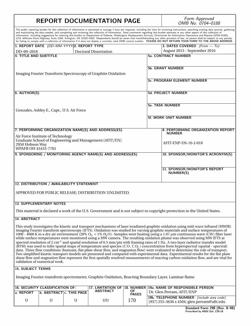
REPORT DOCUMENTATION PAGE Form ApprovedOMB No. 0704–0188
The public reporting burden for this collection of information is estimated to average 1 hour per response, including the time for reviewing instructions, searching existing data sources, gatheringand maintaining the data needed, and completing and reviewing the collection of information. Send comments regarding this burden estimate or any other aspect of this collection ofinformation, including suggestions for reducing this burden to Department of Defense, Washington Headquarters Services, Directorate for Information Operations and Reports (0704–0188),1215 Jefferson Davis Highway, Suite 1204, Arlington, VA 22202–4302. Respondents should be aware that notwithstanding any other provision of law, no person shall be subject to any penaltyfor failing to comply with a collection of information if it does not display a currently valid OMB control number. PLEASE DO NOT RETURN YOUR FORM TO THE ABOVE ADDRESS.
1. REPORT DATE (DD–MM–YYYY)2. REPORT TYPE 3. DATES COVERED (From — To)
4. TITLE AND SUBTITLE 5a. CONTRACT NUMBER
5b. GRANT NUMBER
5c. PROGRAM ELEMENT NUMBER
5d. PROJECT NUMBER
5e. TASK NUMBER
5f. WORK UNIT NUMBER
6. AUTHOR(S)
7. PERFORMING ORGANIZATION NAME(S) AND ADDRESS(ES) 8. PERFORMING ORGANIZATION REPORTNUMBER
9. SPONSORING / MONITORING AGENCY NAME(S) AND ADDRESS(ES) 10. SPONSOR/MONITOR’S ACRONYM(S)
11. SPONSOR/MONITOR’S REPORTNUMBER(S)
12. DISTRIBUTION / AVAILABILITY STATEMENT
13. SUPPLEMENTARY NOTES
14. ABSTRACT
15. SUBJECT TERMS
16. SECURITY CLASSIFICATION OF:
a. REPORT b. ABSTRACT c. THIS PAGE
17. LIMITATION OFABSTRACT
18. NUMBEROFPAGES
19a. NAME OF RESPONSIBLE PERSON
19b. TELEPHONE NUMBER (include area code)
Standard Form 298 (Rev. 8–98)Prescribed by ANSI Std. Z39.18
DD–09–2016 Doctoral Dissertation August 2013 - September 2016
Imaging Fourier Transform Spectroscopy of Graphite Oxidation
Gonzales, Ashley E., Capt., U.S. Air Force
Air Force Institute of TechnologyGraduate School of Engineering and Management (AFIT/EN)2950 Hobson WayWPAFB OH 45433-7765
AFIT-ENP-DS-16-J-018
APPROVED FOR PUBLIC RELEASE; DISTRIBUTION UNLIMITED.
This material is declared a work of the U.S. Government and is not subject to copyright protection in the United States.
This study investigates the kinetic and transport mechanisms of laser irradiated graphite oxidation using mid-wave infrared (MWIR)imaging Fourier transform spectroscopy (IFTS). Oxidation was studied for varying graphite materials and surface temperatures of1000 - 4000 K in a dry air environment (20% O2, < 1% H2O ). Samples were heating using a 1.07 µm continuous wave (CW) fiber laserwhile surface temperatures were monitored using a MW camera. The resulting oxidation plume was observed using MW IFTS atspectral resolution of 2 cm-2 and spatial resolution of 0.5 mm/pix with framing rates of 1 Hz. A two layer radiative transfer model(RTM) was used to infer spatial maps of temperature and species (C O , C O2 ) concentration from hyperspectral (spatial - spectral)data. Three flow conditions (buoyant, flat plate shear flow, and stagnation flow) were evaluated to determine the role of transport.Two simplified kinetic transport models are presented and compared with experimental data. Experimental results for the flat plateshear flow and stagnation flow represent the first spatially resolved measurements of reacting carbon oxidation flow, and are vital forvalidation of numerical work.
Imaging Fourier-transform spectrometer, Graphite Oxidation, Reacting Boundary Layer, Laminar flame
U U U UU 170Dr. Glen Perram, AFIT/ENP
(937) 255-3636 x 4504; [email protected]

![a c arXiv:1701.08267v1 [astro-ph.EP] 28 Jan 2017 · cV.E. Zuev Institute of Atmospheric Optics, SB RAS, 1, Academician Zuev Square, Tomsk 634021, Russia ... and CDSD-296 databases](https://img.pdfslide.us/doc/110x75/5b9f135109d3f25b318c7f96/a-c-arxiv170108267v1-astro-phep-28-jan-2017-cve-zuev-institute-of-atmospheric.jpg)
![Index [banelec.online.fr]banelec.online.fr/fab/kemet/HiTemp HiVolt Ceram Caps.pdf · © KEMET Electronics Corporation • PO Box 5928 • Greenville, SC 29606 • 3 High Temperature,](https://img.pdfslide.us/doc/110x75/5e82f745351c113fa578dcdf/index-hivolt-ceram-capspdf-kemet-electronics-corporation-a-po-box-5928.jpg)