Direct numerical study of speed of sound in dispersedair-water two-phase flow

Kai Fua, Xiao-Long Denga,b,∗, Lingjie Jianga

aBeijing Computational Science Research Center, Beijing 100193, ChinabDepartment of Mechanical and Aerospace Engineering, University of Virginia, VA 22904, USA

Abstract

Speed of sound is a key parameter for the compressibility effects in multiphase flow.We present a new approach to do direct numerical simulations on the speed of soundin compressible two-phase flow, based on the stratified multiphase flow model (Chang& Liou, JCP 2007). In this method, each face is divided into gas-gas, gas-liquid, andliquid-liquid parts via reconstruction of volume fraction, and the corresponding fluxesare calculated by Riemann solvers. Viscosity and heat transfer models are included. Theeffects of frequency (below the natural frequency of bubbles), volume fraction, viscosityand heat transfer are investigated. With frequency 1 kHz, under viscous and isothermalconditions, the simulation results satisfy the experimental ones very well. The simula-tion results show that the speed of sound in air-water bubbly two-phase flow is largerwhen the frequency is higher. At lower frequency, for the phasic velocities, the homo-geneous condition is better satisfied. Considering the phasic temperatures, during thewave propagation an isothermal bubble behavior is observed. Finally, the dispersionrelation of acoustics in two-phase flow is compared with analytical results below thenatural frequency. This work for the first time presents an approach to the direct numer-ical simulations of speed of sound and other compressibility effects in multiphase flow,which can be applied to study more complex situations, especially when it is hard to doexperimental study.

Keywords: Speed of sound; Two-phase; Stratified multiphase flow method;Compressibility effects; Homogeneous flow; Bubble thermodynamics;

1. Introduction

The compressibility can lead to several physical phenomena, such as choked flow andwater hammer. Consider the following equation in one-dimensional (1D) flow,

−M2 du

u=

dρ

ρ(1)

∗Corresponding author.Email addresses: kaifu@csrc.ac.cn (Kai Fu), xiaolong.deng@csrc.ac.cn (Xiao-Long Deng)

March 22, 2018

arX

iv:1

803.

0460

4v2

[ph

ysic

s.fl

u-dy

n] 2

1 M

ar 2

018

where M = u/c is the Mach number. The derivation of Eqn. 1 can be found in AppendixA. From Eqn. 1, we could explain the mass chocking due to compressibility effect,as discussed by Hall (2015). For low subsonic condition flow, M is so small that thecompressibility effects can be ignored. Thus, the increase of flow velocity means theincrease of flow mass flux. As the speed of the object approaches the speed of soundc, the density ρ starts to decrease, and the mass flux increases slower. At the criticalpoint M = 1, the mass flux achieves its maximum value. It is usually noted that thecompressibility effects cannot be ignored when M > 0.3.

In single-phase flow, the critical flow velocity is identical to the speed of sound of thefluid. In general, this relationship cannot apply to multiphase flow since there may bemore than one speed of sound in multiphase flow. However, as discussed by Corradiniet al. (2016), the identity between the critical flow velocity and acoustic velocity ofmixture is preserved in homogeneous equilibrium model (HEM). The model assumesthat: (1) the velocity of each phase is equal, and (2) the phases are in thermodynamicequilibrium. Therefore, the decrease of local speed of sound can result in a decrease oflocal critical mass flux. The critical mass flux of the cooling system is relying on theselocal critical mass flux. For example in 1D case, according to the mass conservation wehave ρuA = const. The critical mass flux of the system is determined by the condition(local critical mass flux) at the minimum A. The decrease of critical mass flux couldlower the heat transfer efficiency in cooling system. Therefore, in nuclear reactor thecompressibility effects can lead to a deteriorated heat transfer efficiency when the fuelassembly encounter a sudden loss of local speed of sound.

Water hammer (or hydraulic shock) is also related to the compressibility effects in thefluid. In cooling system of nuclear power plants, it can cause potential safety problem asintroduced by Beuthe (1997). Water hammer, which is the generation of great variationof pressure along the mass transportation pipe, is caused by the sudden change of localfluid velocity and thus a fatigue failure may occur (see more in Calvert (2000)).

Since the speed of sound is the key factor for compressibility effects, there are alreadyextensive studies on the acoustic behavior of multiphase flow (Karplus (1958); Mecredyand Hamilton (1972); Kieffer (1977); Ardron and Duffey (1978); Cheng et al. (1983);Ruggles et al. (1988); Costigan and Whalley (1997); Drew and Passman (1999); Brennen(2005); Simon et al. (2016); Drui et al. (2016)). In the theoretical study, an analytical ex-pression which supposedly quantified the acoustic behavior in two-phase flow was derivedfrom a 1D two-fluid model. Thanks to the development of high-performance computingin recent years, we are now capable to investigate acoustics of two-phase flow with adirect numerical simulation (DNS) method. In this paper, we studied the propagationof a plane wave in dispersed two-phase flow with the stratified multiphase flow method(Chang and Liou (2007)). The diffuse-interface method (DIM) is applied for the directsimulation of two-phase flow with interfacial momentum and heat transfer.

The paper is structured as follows. First we introduced the theory of acoustics inhomogeneous flow and separated flow. Then the governing equations for DNS study arepresented, in which the viscous effects and heat diffusion are discussed. The stratifiedflow method adopted in the simulation is briefly introduced. The convergence of ournumerical method is discussed. The momentum analysis and bubble thermodynamicsare presented in the context of direct simulation results. Finally we will compare thesimulated acoustic behavior in two-phase flow with both experimental and theoreticalresults.

2

2. Theoretical speed of sound in two-phase flow

In this section, the theory of speed of sound in two-phase flow is discussed. Considerdispersed bubbly flow in pipes, where the volume fraction is treated as constant withposition along the pipe in the scale of grid size. If the size of the dispersed phase ismuch smaller than the wavelength, the two-phase flow resembles a single-phase fluidwith effective acoustic properties as discussed by Dijk (2005). For separated flow, thereare two layers clearly, with the lighter fluid flowing on top of the heavier fluid. And ithas different acoustics from the bubbly flow.

In the following part, we only list the major theoretical conclusion of two-phaseacoustics. The derivation could be found in Appendix B.

2.1. Speed of sound in dispersed homogeneous flow

In dispersed two-phase flow, the relative motion between dispersed and continuousphase could be ignored if the dispersed particles are much smaller than the wavelength,as indicated by Brennen (2005). We will also have a discussion in section 4.2. In thisway, the two-phase flow could be treated as the homogeneous flow.

Consider the quiescent two-phase flow with each component uniform. We have thecontinuity equation,

∂αkρk∂t

+∇ · (αkρkuk) = 0 (2)

Consider the momentum conservation equation in dispersed two-phase flow,

∂αkρkuk

∂t+∇ · (αkρkukuk) = −αk∇p+ Fi (3)

where Fi refers to the interfacial momentum transfer term. Here the surface tension isignored so that the index k could be moved out from pk, as shown in the first term atthe right-hand side (RHS) of Eqn. 3. In homogenous flow, Fi is so large that the relativevelocity is neglected.

Equations. 2 and 3 are linearized and thus the speed of sound in the two-phasehomogenous flow could be written as

1

c2hom

= (αgρg + αlρl)

(αg

ρgc2g+

αl

ρlc2l

)(4)

where

c2k =

(dp

dρk

)Q

(5)

Here Q is the thermodynamic constraint. It is necessary to investigate the energy con-servation equation to specify Q. In gas/liquid two-phase flow, bulk modulus of liquid isusually much larger than that of gas, that is

ρgc2g � ρlc

2l (6)

Thus only cg needs to be considered in Eqn. 4. The term associated with cl can beignored. For ideal gas, we have

cg =

√γgpgρg

(7)

3

where γg = 1.0 for isothermal condition and γg = 1.4 for adiabatic condition. Note thatin homogeneous flow, the isothermal condition is equivalent to HEM we mentioned inthe introduction. The flow has larger speed of sound in adiabatic bubble behavior, whichis also discussed by Fl̊atten et al. (2010). We will have more discussions about this issuein section 4.3.

In summary, the velocity and pressure of both phases are relaxed in homogeneousflow. The speed of sound in this case could be written down as Eqn. 4.

2.2. Speed of sound in separated flow

We take a 1D analysis to investigate the speed of sound in separated flow. Considerquiescent two-phase flow in a long and narrow pipe, the wave propagates along thelongitude direction (x axis). The wavelength is much larger than the diameter of pipe sothat we have isobaric condition at each cross section of the pipe.

The continuity equation for separated flow is the same as Eqn. 2. In each phase, themomentum conservation equation reads

ρk

(∂uk∂t

+ uk∂uk∂x

)= −∂p

∂x(8)

in the longitudinal direction, where it is assumed that the flow is inviscid and there is nointerfacial shear stress. The surface tension is ignored as well.

By linearizing Eqns. 2 and 8, we obtain the speed of sound in separated inviscid flow,

1

c2sep

(αg

ρg+αl

ρl

)=

αg

ρgc2g+

αl

ρlc2l(9)

where ck refers to Eqn. 6.In summary, only the pressure of both phases is relaxed in separated flow. There is

a relative motion between the two phases in the flow. The speed of sound in this casecould be written down as Eqn. 9.

3. Numerical methods

In DIM, an appropriate fluid mixture model has to be proposed to describe (1) equa-tion of interface motion and (2) equation of state for fluid mixture in mixing region. Baerand Nunziato (1986); Zein et al. (2010) proposed the 7-equation model for two-phase flow.The model is a full non-equilibrium model, in which each phase has its own pressure,velocity and temperature. The 6-equation model is derived from the 7-equation modelin the asymptotic limit of stiff velocity relaxation, as discussed in Saurel et al. (2009).The 7-equation or 6-equation model should not be considered as a physical model, butmore as a step-model to solve the 5-equation model, which is introduced in Shyue (1998);Murrone and Guillard (2005). In the 5-equation model, Shyue (2014) discussed that me-chanical equilibrium is assumed, while the thermal and chemical relaxation are frozen.In his work, a comparison of equilibrium speed of sound in steam/water two-phase flowis made under different relaxation limits.

In some practical problems, due to the slow effects of the fluid viscosity, the velocityin tangential direction may have a large relaxation time scale. Therefore in our work, we

4

applied the model which assumes that the velocity of each phase is non-equilibrium. Inthis section, we introduced the stratified multiphase flow method which was implementedin Taiji solver by Chang and Liou (2007). In this method, they studied the compressiblemultifluid equations in which the fluids are assumed inter-penetrating, non-homogeneousand non-equilibrium. That is to say, each fluid has its own velocity and temperature fieldsat the same location, but all fluids share the same pressure.

3.1. Governing equation

First, we introduce the governing equation used in our method. The continuity equa-tion is already introduced as in Eqn. 2. The inviscid Navier-Stokes equation was intro-duced as,

∂(αkρkuk)

∂t+∇ · (αkρkukuk) +∇(αkpk) = pi∇αk (10)

The first and second term in the left-hand side (LHS) is the convection term. Thethird term is similar to the typical pressure interaction term in single-phase flow. TheRHS represents the interfacial momentum transfer term and only includes the pressurecontribution part.

In our method, we assumed that both components have the same pressure, thus

p = pk (11)

Furthermore, we assumed that the interfacial pressure is equal to the pressure of eachfluid, as suggested by Ishii and Hibiki (2011) (p.187),

p = pi (12)

If the viscosity is considered then we finally obtain the momentum conservation equa-tion as

∂(αkρkuk)

∂t+∇ · (αkρkukuk) +∇(αkp)−∇ · (αkτ ) = p∇αk (13)

where τ is the averaged stress,

τ = µ(∇u + (∇u)+)− 2

3µ(∇ · u)I (14)

u =∑k

αkρkuk (15)

µ =∑k

αkρkµk (16)

Chang and Liou (2007) introduced the energy conservation equation for inviscid two-phase flow as,

∂(αkρkek)

∂t+∇ · (αkρkekuk) +∇ · (αkpuk) = −p∂αk

∂t(17)

where ek refers to the virtual internal energy of phase k which includes the standardthermal energy and the turbulent kinetic energy (see more in Ishii and Hibiki (2011)).

5

The first and second term in LHS of Eqn. 17 is the convection term. The third term issimilar to the work done by pressure in single-phase flow. The RHS represents the workdone by interfacial pressure to phase k due to its volume change.

Equation 17 is applied to inviscid two-phase flow without heat conduction. Further-more considering the viscosity and heat conduction, we have the energy conservationequation as,

∂(αkρkek)

∂t+∇ · (αkρkekuk) +∇ · (αk(pI− τ ) · u) +∇ · (αkq′′) = −p∂αk

∂t(18)

where the average heat flux is calculated with the Fourier’s law,

q′′ = −k∇T (19)

Here the average conductivity of mixture is calculated as

k =∑k

αkρkkk (20)

and the average temperature of mixture

T =

∑k

αkρkcpkTk∑k

αkρkcpk(21)

In Eqn. 18, we simply assign αk as the ratio that phase k obtained from the conduc-tion heat flux q′′. The method was not strictly developed from two-phase model and theaccurate modelling of heat conduction in two-phase flow is beyond scope of this work.

It is suggested by Brennen (2005) that the isothermal bubble behavior is more favor-able during wave propagation. Therefore, similar to the work done by Fu and Anglart(2017), we add an additional source term and rewrite Eqn. 18 as

∂(αkρkek)

∂t+∇ · (αkρkekuk) +∇ · (αk(pI− τ ) · u) +∇ · (αkq′′) = −p∂αk

∂t+ Sk (22)

where Sk is the source term to keep gas at constant temperature,

Sg =αgρg∆t

cpg(Tref − Tg) (23)

Here Tref is the reference temperature and ∆t is numerical time step. To preserve theconservation of energy, we have

Sl = −Sg (24)

We call Eqn. 18 as thermal model 1 (TM1) and call Eqn. 22 as thermal model 2(TM2). Both models are studied in the simulation.

In summary, Eqns. 2, 13 and 22 are used as the governing equations in our simulation.

6

𝑊𝑊

𝜌𝜌2𝑢𝑢2𝑝𝑝2

𝜌𝜌1𝑢𝑢1 = 0𝑝𝑝1

0

𝜌𝜌2𝑢𝑢2 −𝑊𝑊𝑝𝑝2

𝜌𝜌1−𝑊𝑊𝑝𝑝1

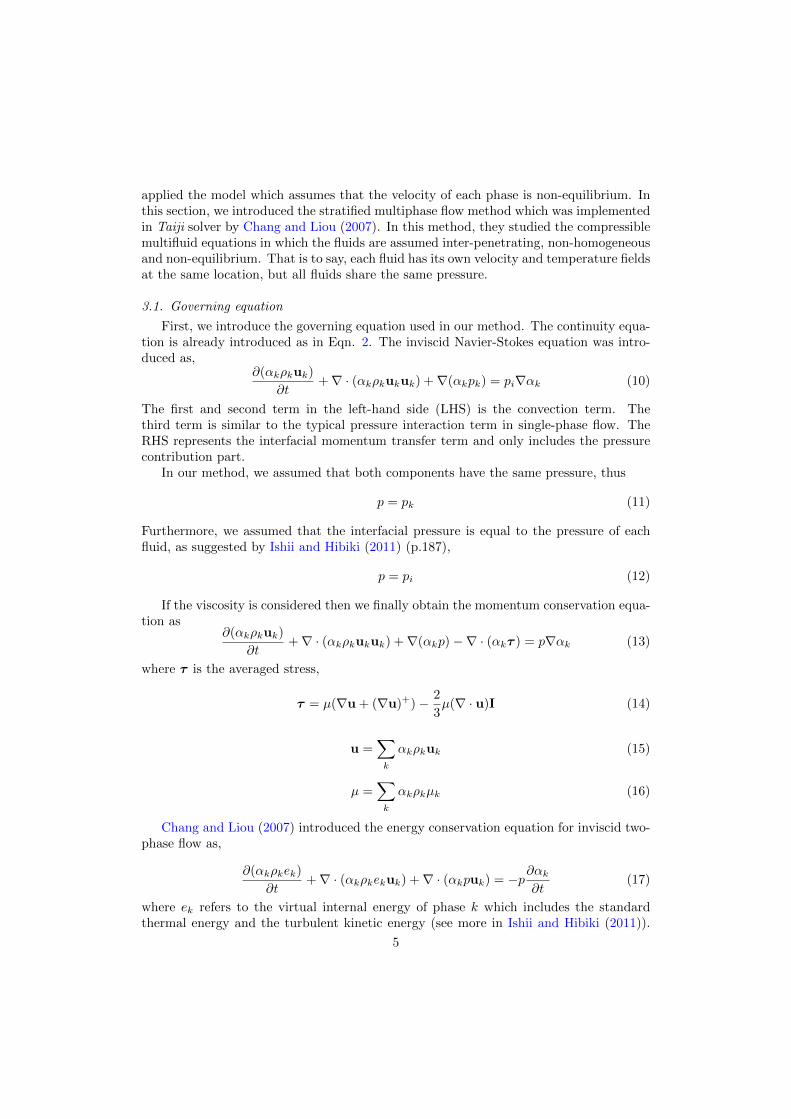
(a) (b)Figure 1: Right-facing shock wave: (a) stationary frame of reference, shock has speed W ; (b) frame ofreference moves with speed W , so that the shock has zero speed

3.2. Perturbation boundary condition

To investigate the wave propagation, we have to setup an appropriate boundary con-dition which represents the vibration source. Naturally we would like to setup a boundarycondition with a harmonic perturbation. The perturbation condition we applied here areobtained from the Rankine-Hugoniot condition, as discussed by Toro (2009) and Ranjanet al. (2011). Consider the Rankine-Hugoniot condition for a shock. It is found conve-nient to transform the problem to a new frame of reference moving with the shock sothat in the new frame the shock speed is zero. Figure 1 depicts both frames of reference.

Consider the inviscid flow, which is adiabatic across the shock wave in Fig. 1b. Thefollowing equations read,

ρ1W = ρ2(W − u2) (25)

p1 + ρ1W2 = p2 + ρ2(W − u2)2 (26)

h1 +1

2W 2 = h2 +

1

2(W − u2)2 (27)

Here subscript 1 refers to the wave front and subscript 2 the post-shock. W is theinterface moving velocity, or wave velocity. The stiffened-gas model used in Bai andDeng (2017) is applied as equation of state (EOS) for fluids, as

pk(ρk, Tk) =γk − 1

γkcpkρkTk − p∞,k (28)

where cpk is the specific heat capacity of phase k at constant pressure. And,

hk(ρk, Tk) ≡ ek +pkρk

= cpkTk (29)

The relevant parameters for both phases are listed in Table 1.

Table 1: Parameter for stiffened-gas model

fluid γ cp ( J/(kg ·K)) p∞ (Pa)water 2.788103 4190.0 7.86253× 108

air 1.4 1008.7 0

7

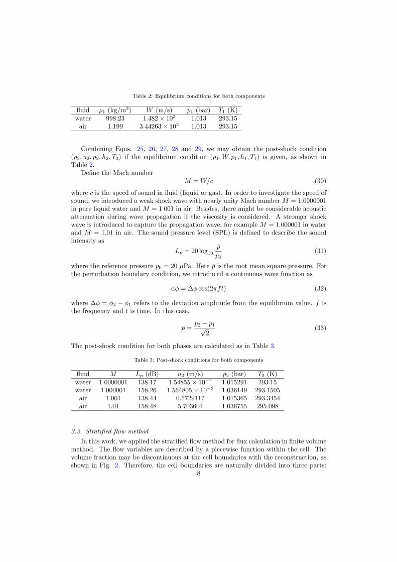
Table 2: Equilibrium conditions for both components

fluid ρ1 (kg/m3) W (m/s) p1 (bar) T1 (K)water 998.23 1.482× 103 1.013 293.15

air 1.199 3.44263× 102 1.013 293.15

Combining Eqns. 25, 26, 27, 28 and 29, we may obtain the post-shock condition(ρ2, u2, p2, h2, T2) if the equilibrium condition (ρ1,W, p1, h1, T1) is given, as shown inTable 2.

Define the Mach numberM = W/c (30)

where c is the speed of sound in fluid (liquid or gas). In order to investigate the speed ofsound, we introduced a weak shock wave with nearly unity Mach number M = 1.0000001in pure liquid water and M = 1.001 in air. Besides, there might be considerable acousticattenuation during wave propagation if the viscosity is considered. A stronger shockwave is introduced to capture the propagation wave, for example M = 1.000001 in waterand M = 1.01 in air. The sound pressure level (SPL) is defined to describe the soundintensity as

Lp = 20 log10

p̄

p0(31)

where the reference pressure p0 = 20 µPa. Here p̄ is the root mean square pressure. Forthe perturbation boundary condition, we introduced a continuous wave function as

dφ = ∆φ cos(2πft) (32)

where ∆φ = φ2 − φ1 refers to the deviation amplitude from the equilibrium value. f isthe frequency and t is time. In this case,

p̄ =p2 − p1√

2(33)

The post-shock condition for both phases are calculated as in Table 3.

Table 3: Post-shock conditions for both components

fluid M Lp (dB) u2 (m/s) p2 (bar) T2 (K)water 1.0000001 138.17 1.54855× 10−4 1.015291 293.15water 1.000001 158.26 1.564805× 10−3 1.036149 293.1505

air 1.001 138.44 0.5729117 1.015365 293.3454air 1.01 158.48 5.703604 1.036755 295.098

3.3. Stratified flow method

In this work, we applied the stratified flow method for flux calculation in finite volumemethod. The flow variables are described by a piecewise function within the cell. Thevolume fraction may be discontinuous at the cell boundaries with the reconstruction, asshown in Fig. 2. Therefore, the cell boundaries are naturally divided into three parts:

8

Gas

Liquid

Gas

Liquid

𝜃𝜃𝑙𝑙−𝑔𝑔

𝜃𝜃𝑔𝑔−𝑔𝑔

𝜃𝜃𝑙𝑙−𝑙𝑙

Figure 2: Illustration of 1D stratified flow model

gas-gas interface (θg−g), liquid-gas interface (θl−g or θg−l) and liquid-liquid interface(θl−l). In stratified flow model, the interface flux between different phases can be calcu-lated at the cell boundaries. The AUSM+-up scheme was introduced for the liquid-liquidor gas-gas flux calculation at cell interface and the exact Riemann solver was used tocalculate the liquid-gas flux at cell interface. More details of the method can be foundin Chang and Liou (2007).

3.4. Configuration setup

In this section, we introduce the configuration of calculation domain. It is a two-dimensional (2D) rectangle (l1 × l2). Usually the length l1 should cover several wave-length, and the width l2 is equal to several bubble diameter. The calculation domainwas designed with the two-phase mixture zone in the center and the single-phase zoneat both sides.

Figure 3 is a typical configuration in our simulation case. The liquid-gas mixturezone locates in 30×3 mm2. Both top and bottom edges were applied for periodic bound-ary condition. The inlet was setup with the perturbation condition as we introducedin Eqn. 32, and outlet with free stream boundary condition. More specifically, in caseof liquid continuum, the inlet condition is applied with perturbation condition of water.And in case of gas continuum, the perturbation condition of air was applied for inletboundary condition. The dispersed phase, either liquid or gas, is randomly distributedin the mixture zone with the same diameter. The distance between centers of two arbi-trary bubbles/droplets should satisfy the following relationship to ensure well-distributedparticles,

l ≥ εD (34)

where ε > 1.0 is a controlling parameter, for example ε = 1.03 if αg = 0.5 and ε = 1.3if αg = 0.3. In the other way, the particles are regularly aligned in the mixture zone forcomparison. The number of particles is calculated by

N =4αdS

πD2(35)

where S is the area of mixture zone.The DIM is used in our work. The interface separating the two phases is captured by

φ, which is defined as a signed distance from the interface. The negative sign is chosen

9

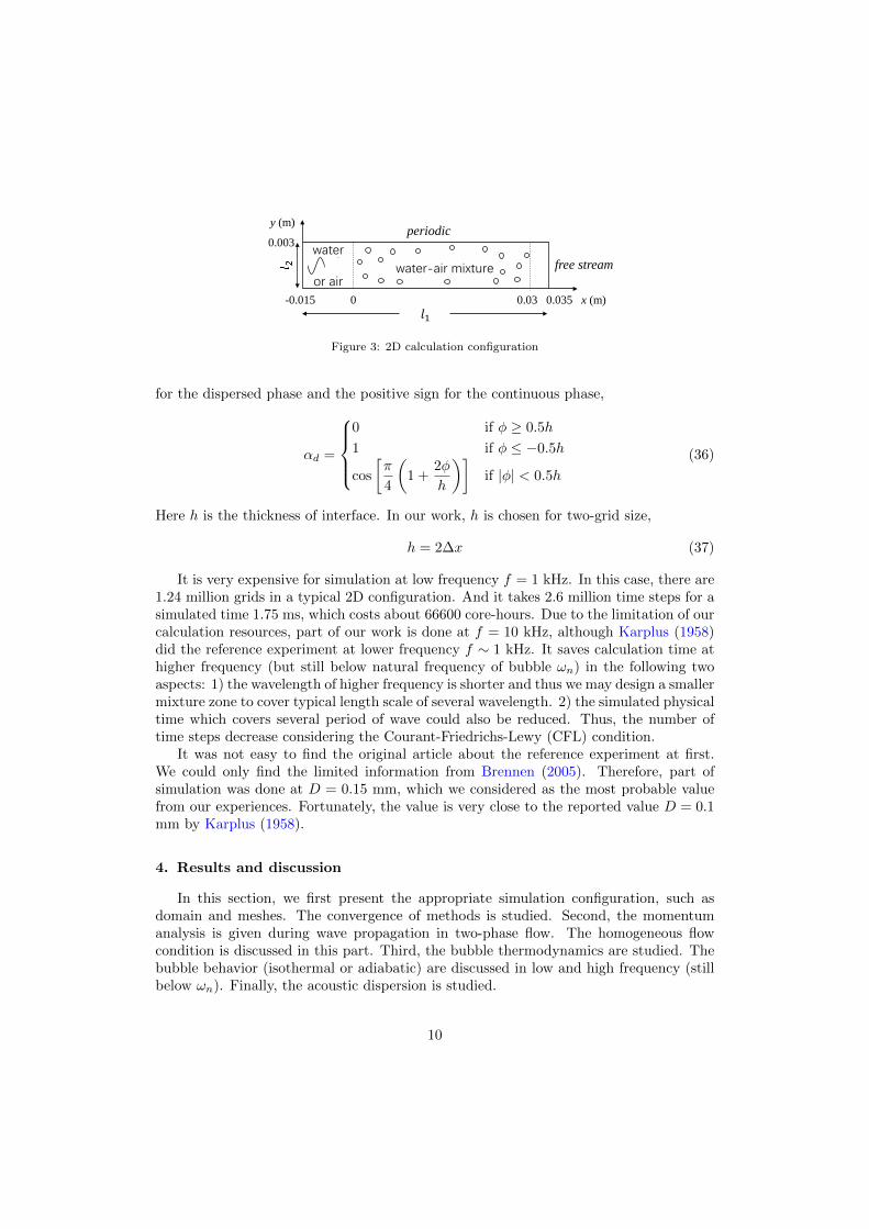
water

or airwater-air mixture

-0.015 0 0.03 0.035 x (m)

y (m)

0.003periodic

free stream

𝑙𝑙1

Figure 3: 2D calculation configuration

for the dispersed phase and the positive sign for the continuous phase,

αd =

0 if φ ≥ 0.5h

1 if φ ≤ −0.5h

cos

[π

4

(1 +

2φ

h

)]if |φ| < 0.5h

(36)

Here h is the thickness of interface. In our work, h is chosen for two-grid size,

h = 2∆x (37)

It is very expensive for simulation at low frequency f = 1 kHz. In this case, there are1.24 million grids in a typical 2D configuration. And it takes 2.6 million time steps for asimulated time 1.75 ms, which costs about 66600 core-hours. Due to the limitation of ourcalculation resources, part of our work is done at f = 10 kHz, although Karplus (1958)did the reference experiment at lower frequency f ∼ 1 kHz. It saves calculation time athigher frequency (but still below natural frequency of bubble ωn) in the following twoaspects: 1) the wavelength of higher frequency is shorter and thus we may design a smallermixture zone to cover typical length scale of several wavelength. 2) the simulated physicaltime which covers several period of wave could also be reduced. Thus, the number oftime steps decrease considering the Courant-Friedrichs-Lewy (CFL) condition.

It was not easy to find the original article about the reference experiment at first.We could only find the limited information from Brennen (2005). Therefore, part ofsimulation was done at D = 0.15 mm, which we considered as the most probable valuefrom our experiences. Fortunately, the value is very close to the reported value D = 0.1mm by Karplus (1958).

4. Results and discussion

In this section, we first present the appropriate simulation configuration, such asdomain and meshes. The convergence of methods is studied. Second, the momentumanalysis is given during wave propagation in two-phase flow. The homogeneous flowcondition is discussed in this part. Third, the bubble thermodynamics are studied. Thebubble behavior (isothermal or adiabatic) are discussed in low and high frequency (stillbelow ωn). Finally, the acoustic dispersion is studied.

10

0 10 20 30 40 50 6020

25

30

35

40

Cal

cula

ted

soni

c ve

loci

ty (

m/s

)

Sensitivity study for grids size

138.17 dB158.26 dB

Figure 4: Sensitivity test for grid resolution and sound intensity Lp

mm

(a)

𝑙𝑙1 = 2 cm

mm

(b)

Figure 5: Comparison of velocity field between (a) randomly distributed and (b) aligned gas bubbles

4.1. Convergence of numerical methods and sensitivity study

First, considering the calculation efficiency, appropriate size of domain and grid shouldbe determined. Considering the periodic boundary condition in y direction, l2 = 5D isused in this work. The reasonable grid size ∆x, which should be sufficient to capture thegas-liquid interface, is chosen to save the calculation time. The sensitivity study aboutthe resolution D/∆x is shown in Fig. 4. The result shows that the wave propagationspeed has the first order convergence. Thus, it is reasonable for us to choose D/∆x = 20in the calculation. We also did the sensitivity study to the intensity of sound Lp. Itis found that sometimes the wave was too weak to be captured. Thus, we used in oursimulation the strong shock wave condition as listed in Table. 3. Obviously, we obtainthe same speed of sound for both weak and strong condition, as shown in Fig. 4.

The distribution pattern of particles is studied in this work. Figure 5 shows thevelocity field of flow in different distribution pattern of dispersed phase, at the sametime t = 3 × 10−4 s, where α = 0.02, D = 0.15 mm and f = 10 kHz. The similartwo regular flow patterns indicate the waves almost have the same propagation speed.Further investigation shows that c = 76.4 m/s for random pattern in Fig. 5a and c = 75.3m/s for aligned pattern in Fig. 5b.

11

0 0.2 0.4 0.6 0.8 10

100

200

300

400

500

600

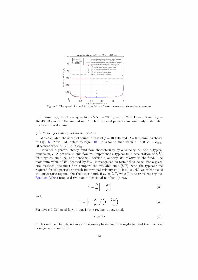
Figure 6: The speed of sound in a bubbly air/water mixture at atmospheric pressure

In summary, we choose l2 = 5D, D/∆x = 20, Lp = 158.26 dB (water) and Lp =158.48 dB (air) for the simulation. All the dispersed particles are randomly distributedin calculation domain.

4.2. Sonic speed analysis with momentum

We calculated the speed of sound in case of f = 10 kHz and D = 0.15 mm, as shownin Fig. 6. Note TM1 refers to Eqn. 18. It is found that when α → 0, c → chom.Otherwise when α→ 1, c→ csep.

Consider a general steady fluid flow characterized by a velocity, U , and a typicaldimension, l. A particle in this flow will experience a typical fluid acceleration of U2/lfor a typical time l/U and hence will develop a velocity, W , relative to the fluid. Themaximum value of W , denoted by Wm, is recognized as terminal velocity. For a givencircumstance, one must first compare the available time (l/U), with the typical timerequired for the particle to reach its terminal velocity (tu). If tu � l/U , we refer this asthe quasistatic regime. On the other hand, if tu � l/U , we call it as transient regime.Brennen (2005) proposed two non-dimensional numbers (p.78),

X =D

2l

∣∣∣∣1− ρdρc

∣∣∣∣ (38)

and,

Y =

∣∣∣∣1− ρdρc

∣∣∣∣/(1 +2ρdρc

)(39)

For inviscid dispersed flow, a quasistatic regime is suggested,

X � Y 2 (40)

In this regime, the relative motion between phases could be neglected and the flow is inhomogeneous condition.

12

In dispersed air/water two-phase flow, the typical length is wavelength. From Eqns.38, 39 and 40, the homogeneous condition is satisfied if

D

2λ

(1− ρg

ρl

)� 1 (41)

Take a typical simulation case for the dispersed air/water mixture, D = 1.0 × 10−4 m,and λ = 2.5×10−3 m. In this condition, Eqn. 41 is satisfied and the flow is homogeneous.

However, in dispersed water/air two-phase flow, the density of water droplet is muchlarger than that of air. The homogeneous condition is not satisfied any more. From Fig.6, we have chom < c < csep (here c is the simulated speed of sound in gas continuum),which indicates that the relative motion could not be ignored. One interesting thingcould be found in the case α = 0.5. With the same volume fraction, the simulatedspeed of sound in liquid continuum is different from the one in gas continuum. It isdue to the shape effects on drag. In dispersed air/water mixture, the gas bubbles arespherical. They are easily accelerated by drag force due to their light density. Thus, theterminal velocity could be reached instantly and we say that the two-phase flow is inthe quasistatic regime. However, in the dispersed water/air mixture, the liquid dropletsare spherical. The acceleration of the droplet is not so easy and it takes a long timefor droplet to reach the terminal velocity. The two-phase flow is then in the transitionregime and homogenous condition is not satisfied.

4.3. Sonic speed analysis with bubble thermodynamics

Due to large heat capacity, Tl is almost constant at the equilibrium temperatureTe = 293.15 K,

Tl ≈ Te (42)

In TM1, Tg could be varied from Te due to the compression and rarefaction accompanyingthe passage of the sound wave. In what follows, we discuss the heat diffusion problemwhich is important to bubble thermodynamics in two-phase flow.

First, we consider a 1D heat conduction problem in single-phase flow, and heat dif-fusion in two-phase flow is quite analogous.

1

r2

∂

∂r(r2 ∂T

∂r) =

1

κ

∂T

∂t(43)

The analytic solution can be found in Ernesto (2006). The characteristic diffusive length

ld =√κτ (44)

is introduced during the typical time τ = 1/f . Comparing ld with the wavelengthλ = c/f , as shown in Fig. 7a, the relaxation frequency

ftc,1Φ =c2

κ(45)

for thermal conduction is introduced to determine fluid condition during wave propaga-tion: isentropic or isothermal. Dijk (2005) pointed out that for single-phase flow in thelow frequency f � ftc,1Φ, the equilibrium speed of sound is given as

c2s =

(dp

dρ

)s

(46)

13

(a)

寸 寸

𝑙𝑙𝑑𝑑

𝜆𝜆

𝑝𝑝

𝑥𝑥

𝐷𝐷𝑙𝑙𝑑𝑑

(b)𝑝𝑝

𝑥𝑥

Figure 7: Illustration of gas thermodynamics in wave propagation: diffusion of thermal energy in (a)single-phase flow and (b) two-phase flow

for isentropic condition. In the high frequency f � ftc,1Φ, the conduction of heat fullydominates the energy balance. In this case the frozen speed of sound is given by,

c2T =

(dp

dρ

)T

(47)

for isothermal condition.The above discussion is valid for single-phase flow. For dispersed two-phase flow,

considering bulk modulus of liquid is usually much larger than that of gas, the acousticsare majorly dependent on the gas thermodynamics. In air/water two-phase flow, theaccumulated gas temperature due to compression or decompression is diffused into thesurrounding liquid from the interface, as shown in Fig. 7b. The critical frequency is thengiven by

ftc,TP =κdD2

(48)

where κd is the thermal diffusivity of dispersed phase. For air/water mixture at Te =293.15 K, κg = 1.9 × 10−5 m2/s, D = 1 × 10−4 m, thus ftc,TP ∼ 1 kHz. The air is inthe isothermal condition during wave propagation if f � 1 kHz, which is different fromsingle-phase flow. In section 2.1, we mentioned that γg = 1.0 for isothermal conditionand γg = 1.4 for adiabatic condition. Here ftc,TP indicates which condition, isothermalor adiabatic, that bubbles experience. In air/water mixture, we have

γg =

{1.0 if f � ftc,TP

1.4 if f � ftc,TP

(49)

14

0 0.2 0.4 0.6 0.8 10

20

40

60

80

100

Figure 8: The speed of sound in a bubbly air/water mixture at atmospheric pressure

Figure 8 shows the speed of sound in air/water mixture with f = 1 kHz. TM1and TM2 refer to Eqns. 18 and 22 respectively. First, the result shows that with f = 1kHz, the calculated sonic velocity agrees better with the theoretical prediction, comparedwith f = 10 kHz. It could be explained by the homogeneous condition in low frequency,as indicated in Eqn. 41. Second, consider the case with α = 0.31. According to theexperimental measurement, the simulation result in TM2 is better than in TM1. Itshows that the gas bubbles are more favorable in isothermal condition than in adiabaticcondition. We introduced the heat transfer between two phases in TM1. However furtherinvestigation of the gas temperature shows that the bubbles have a small temperaturevariation either by compression or decompression. Therefore, we consider TM1 simulatean adiabatic process roughly. The result with α = 0.5 also shows an isothermal bubblebehavior during wave propagation.

4.4. Acoustic dispersion

The acoustic dispersion relation was derived from the linearized conservation equa-tions and the Rayleigh equation during the past few decades (Mecredy and Hamilton(1972); Ardron and Duffey (1978); Cheng et al. (1983, 1985); Ruggles et al. (1988, 1989);Drui et al. (2016)). In these work, a 1D two-fluid model was used to predict the mea-surement. The model includes bubble dynamics, viscous flow effects and interfacial heattransfer. The dependent variables in this model are space/time averaged variables. AsCheng et al. (1985) discussed, the length scale is large compared to bubble radius and theinter-bubble distance but is small compared to the wavelength, which makes differencefrom DNS method. In quiescent two-phase flow, the pressure drag force could be ignoredsince the relative velocity is zero. The virtual mass force dominates the interfacial mo-mentum transfer. Cheng et al. (1983) studied the effect of the virtual mass coefficientcVM. In his work, the frequency dependent phase velocity is given by,

cph =

(

αg

ρgc2g(1− ω2/ω2n)

+αl

ρlc2l

)(ρg + ρ̄

cVM

αl

)αlρgρl

+αg

1− ω2/ω2n

+

(1 +

αg

αl(1− ω2/ω2n)

)cVM

−1/2

(50)

15

whereρ̄ = αgρg + αlρl (51)

is the average density and

ωn =2

D

(3γgp

ρl+

12γgσ − 4σ

ρlD

)1/2

(52)

is the natural frequency of a pulsating bubble. The evaluation of Eqn. 50 leads to thetypical sonic velocity,

cph =

cl if ω →∞, αg � 1

chom if ω � ωn, cVM →∞csep if ω � ωn, cVM = 0

(53)

Drui et al. (2016) proposed a two-fluid model that accounts for two-scale kinematiceffects: bulk kinematics and small-scale vibrations. Two relaxation parameters relatedto mechanical equilibrium between materials are identified in the model: micro-inertialν and micro-viscosity ε. The evaluation of ν and ε is notable as it could be replaced byinfinitely fast relaxation processes as studied in Saurel et al. (2009); Shyue (2014). The4-equation model is derived for ν → 0 and ε = O(1), in which the dispersion relation isgiven as, (

kε(ω)

ω

)2

=iεω + c−2

homH

iεc2Frozenω +H, cεph(ω) = Re

[ω

kε(ω)

](54)

wherec2Frozen =

αgρgρ̄

c2g +αlρlρ̄c2l (55)

and

H =ρgρlc

2gc

2l

αgαlρ̄(56)

The acoustic dispersion is also studied in our work. It can be related to the followingtwo aspects. The first is the non-equilibrium effects. Brennen (2005) discussed thatwhen the acoustic excitation (or driving) frequency approaches the natural (or resonant)frequency of the bubbles, the bubbles are not in dynamic equilibrium. The EOS we usedto calculate c in single-phase fluid (such as Eqn. 7) does not establish any more. Karplus(1958) estimated that a bubble of 0.1 mm in diameter has the natural frequency f = 55kHz. Fox et al. (1995) calculated the sound velocity in air/water mixture in function offrequency. In their conclusion, it shows that very little dispersion is expected in our casesince the operation frequency (∼ 1 kHz) is far below the resonant frequency (∼ 55 kHz).

The second reason comes from the relative motion which is ignored in the homoge-neous flow model. That is the explanation for dispersion below natural frequency ωn.In fact, Eqn. 41 is not satisfied with high frequency. Wijngaarden (1976) formulatedthe sound velocity in an approximate manner when there exists relative motion. In hisformulation, there will be a larger sound velocity if relative motion exists. Our simulationresults in Fig. 9 agree with the conclusion. In our method, Eqn. 13 promises there couldbe sufficient momentum exchange between phases, but the equality of phasic velocity uk

is not necessary.16

0 3 6 9 12 150

20

40

60

80

100

120

140

160

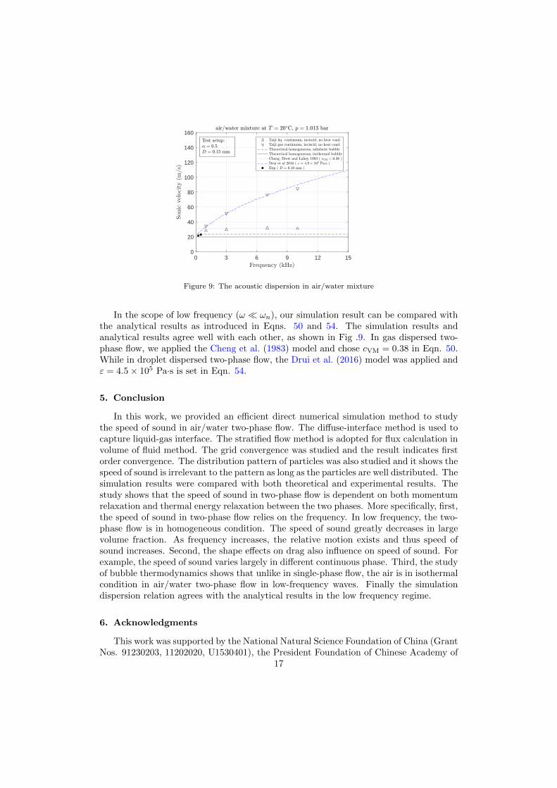
Figure 9: The acoustic dispersion in air/water mixture

In the scope of low frequency (ω � ωn), our simulation result can be compared withthe analytical results as introduced in Eqns. 50 and 54. The simulation results andanalytical results agree well with each other, as shown in Fig .9. In gas dispersed two-phase flow, we applied the Cheng et al. (1983) model and chose cVM = 0.38 in Eqn. 50.While in droplet dispersed two-phase flow, the Drui et al. (2016) model was applied andε = 4.5× 105 Pa·s is set in Eqn. 54.

5. Conclusion

In this work, we provided an efficient direct numerical simulation method to studythe speed of sound in air/water two-phase flow. The diffuse-interface method is used tocapture liquid-gas interface. The stratified flow method is adopted for flux calculation involume of fluid method. The grid convergence was studied and the result indicates firstorder convergence. The distribution pattern of particles was also studied and it shows thespeed of sound is irrelevant to the pattern as long as the particles are well distributed. Thesimulation results were compared with both theoretical and experimental results. Thestudy shows that the speed of sound in two-phase flow is dependent on both momentumrelaxation and thermal energy relaxation between the two phases. More specifically, first,the speed of sound in two-phase flow relies on the frequency. In low frequency, the two-phase flow is in homogeneous condition. The speed of sound greatly decreases in largevolume fraction. As frequency increases, the relative motion exists and thus speed ofsound increases. Second, the shape effects on drag also influence on speed of sound. Forexample, the speed of sound varies largely in different continuous phase. Third, the studyof bubble thermodynamics shows that unlike in single-phase flow, the air is in isothermalcondition in air/water two-phase flow in low-frequency waves. Finally the simulationdispersion relation agrees with the analytical results in the low frequency regime.

6. Acknowledgments

This work was supported by the National Natural Science Foundation of China (GrantNos. 91230203, 11202020, U1530401), the President Foundation of Chinese Academy of

17

Engineering Physics (Grant No. 201501043) and the China Postdoctoral Science Foun-dation (Grant No. 2016M591059). We acknowledge the computational supports from theSpecial Program for Applied Research on Super Computation of the NSFC-GuangdongJoint Fund (the second phase) under Grant No.U1501501, and from the Beijing Compu-tational Science Research Center (CSRC). The authors also thank Dr. Chih-Hao Changfor the fruitful supports and helpful discussions.

18

Nomenclature

A area of cross section, m2

c speed of sound, m·s−1

cp specific heat capacity, J·kg−1·K−1

D diameter, me internal energy, J·kg−1

f driving frequency, Hzh enthalpy, J·kg−1; or interface thickness, mK bulk modulus, N·m−2

k thermal conductivity, W·m−1·K−1

Lp sound pressure level, dBl length, mM Mach numberp pressure, Pap0 reference pressure, PaQ heat, J; or thermodynamic constraintq′′ heat flux, W·m−2

R specific gas constant, J·kg−1·K−1

S area, m2

T temperature, Kt time, stu typical time for particle to reach its terminal velocity, sU typical velocity, m·s−1

u, u velocity, m·s−1

W interface velocity or relative velocity, m·s−1

X non-dimensional numberY non-dimensional number∆x grid size, m

Greek lettersα volume fractionε parameterγ specific heat ratioκ thermal diffusivity, m2·s−1

λ wavelength, mµ dynamic viscosity, kg·m−1·s−1

ν micro-inertia, kg ·m−1

ω angular frequency, s−1

φ signed distance, mρ density, kg·m−3

σ interfacial tension, N·m−1

19

τ stress tensor, N·m−2

τ typical time, sε micro-viscosity, Pa·s

Superscripts′ perturbation

Subscripts1 dispersed phase or wave front1Φ single-phase2 continuous phase or post wavec continuousd dispersed or diffusivee equilibriumg gashom homogeneousi interphasek phasel liquidm maximumn naturalph phases isentropicsep separatedT isothermalTP two-phasetc thermal conduction∞ far field

Appendix A. The derivation of equation in 1D compressible flow

Consider a 1D inviscid flow as show in Fig. A.10, the continuity equation can bewritten down as,

A∂ρ

∂t+

∂

∂x(ρAu) = 0 (A.1)

where u is the averaged flow velocity along x axis and A is the cross-section area.The momentum equation can be written down as,

A∂

∂t(ρu) +

∂

∂x

(ρAu2

)= −A∂p

∂x(A.2)

Combining Eqns. A.1 and A.2, we simply obtain

ρu∂u

∂x= −∂p

∂x(A.3)

for steady flow. The detailed derivation of Eqns. A.1 and A.2 can be found in Hdaneshyar(1976).

20

𝑢𝑢

Area 𝐴𝐴

𝑥𝑥

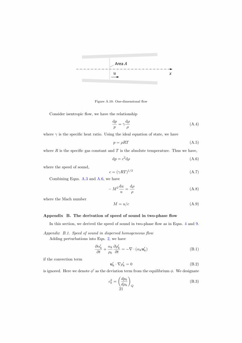
Figure A.10: One-dimensional flow

Consider isentropic flow, we have the relationship

dp

p= γ

dρ

ρ(A.4)

where γ is the specific heat ratio. Using the ideal equation of state, we have

p = ρRT (A.5)

where R is the specific gas constant and T is the absolute temperature. Thus we have,

dp = c2dρ (A.6)

where the speed of sound,c = (γRT )1/2 (A.7)

Combining Eqns. A.3 and A.6, we have

−M2 du

u=

dρ

ρ(A.8)

where the Mach numberM = u/c (A.9)

Appendix B. The derivation of speed of sound in two-phase flow

In this section, we derived the speed of sound in two-phase flow as in Eqns. 4 and 9.

Appendix B.1. Speed of sound in dispersed homogeneous flow

Adding perturbations into Eqn. 2, we have

∂α′k∂t

+αk

ρk

∂ρ′k∂t

= −∇ · (αku′k) (B.1)

if the convection termu′k · ∇ρ′k = 0 (B.2)

is ignored. Here we denote φ′ as the deviation term from the equilibrium φ. We designate

c2k =

(dpkdρk

)Q

(B.3)

21

where Q is the thermodynamic constraint. As Brennen (2005) suggested (p223), in mostpractical circumstances, we have the equilibrium local pressure for both components ifthe surface tension is neglected,

p = p1 = p2 (B.4)

Therefore, the subscript of pressure could be omitted.Substituting Eqn. B.3 into Eqn. B.1, we have

∂α′k∂t

+αk

ρkc2k

∂p′

∂t= −∇ · (αku′k) (B.5)

Then combining Eqn. B.5 for both phases, we have

∂p′

∂t= −K∇ · u′ (B.6)

where we define the effective modulus of the two-phase medium K as

1

K=α1

K1+α2

K2(B.7)

Here Kk = ρkc2k refers to the bulk modulus of each phase. And the bulk velocity fluctu-

ation

u′ = α1u′1 + α2u

′2 (B.8)

The LHS of Eqn. B.6 refers to the change of pressure, and RHS is related to the changeof volume.

In homogenous flow, the interfacial forces Fi in Eqn. 3 are so large that the relativevelocity is neglected, thus we have

u = u1 = u2 (B.9)

Combining Eqn. 3 for both phases, we have

∂ρu

∂t+∇ · (ρuu) = −∇p (B.10)

whereρ = α1ρ1 + α2ρ2 (B.11)

Applying perturbation to Eqn. B.10, and neglecting the convection term, we have

ρ∂u′

∂t+∇p′ = 0 (B.12)

Combining Eqns. B.6 and B.12, we obtain the following wave equation

∂2p′

∂t2=K

ρ∇2p′ (B.13)

Therefore, the speed of sound in the two-phase homogenous flow could be written as

1

c2hom

= (α1ρ1 + α2ρ2)

(α1

ρ1c21+

α2

ρ2c22

)(B.14)

22

Appendix B.2. Speed of sound in separated flow

In separated flow, we already mentioned the isobaric condition at each cross sectionof the pipe. Therefore, the subscript for pressure could also be omitted in this case.

The analysis of continuity equation is the same as in homogeneous flow. ThereforeEqn. B.6 is also applied in this case. The major difference comes from the momentumequation as in Eqn. 8.

Applying perturbation to Eqn. 8, we obtain

ρk∂u′k∂t

= −∂p′

∂x(B.15)

Combining Eqn. B.15 for both phases,

∂u′

∂t= −1

ρ

∂p′

∂x(B.16)

where1

ρ=α1

ρ1+α2

ρ2(B.17)

Combining Eqns. B.6 and B.16, we obtain the speed of sound in inviscid separatedflow as,

1

c2sep

(α1

ρ1+α2

ρ2

)=

α1

ρ1c21+

α2

ρ2c22(B.18)

where ck is specified in Eqn. B.3.

References

Ardron, K.H., Duffey, R.B., 1978. Acoustic wave propagation in a flowing liquid-vapour mixture. Inter-national Journal of Multiphase Flow 4, 303–322.

Baer, M.R., Nunziato, J.W., 1986. A two-phase mixture theory for the deflagration-to-detonation tran-sition (ddt) in reactive granular materials. International Journal of Multiphase Flow 12, 861–889.

Bai, X., Deng, X., 2017. A sharp interface method for compressible multi-phase flows based on the cutcell and ghost fluid methods. Advances in Applied Mathematics and Mechanics 9, 1052–1075.

Beuthe, T.G., 1997. Review of two-phase water hammer, in: Proceedings of the 18th Canadian NuclearSociety Conference, Toronto, Canada.

Brennen, C.E., 2005. Fundamentals of multiphase flows. Cambridge University Press.Calvert, J.B., 2000. Water hammer. https://mysite.du.edu/˜jcalvert/tech/fluids/

waterham.htm. [Online; accessed 03-March-2017].Chang, C., Liou, M., 2007. A robust and accurate approach to computing compressible multiphase flow:

Stratified flow model and ausm+-up scheme. Journal of Computational Physics 225, 840–873.Cheng, L.Y., Drew, D.A., Lahey, R.T., 1983. An analysis of wave dispersion, sonic velocity, and critical

flow in two-phase mixtures. Technical Report NUREG/CR-3372. Rensselaer Polytechnic Institute.URL: https://ntrl.ntis.gov/NTRL/.

Cheng, L.Y., Drew, D.A., Lahey, R.T., 1985. An analysis of wave propagation in bubbly two-component,two-phase flow. Journal of Heat Transfer 107, 402–408.

Corradini, M.L., Zhu, C., Fan, L., Jean, R., 2016. Multiphase flow, in: Johnson, R.W. (Ed.), Handbookof Fluid Dynamics. CRC Press, Boca Raton. chapter 20.

Costigan, G., Whalley, P.B., 1997. Measurements of the speed of sound in air-water flows. ChemicalEngineering Journal 66, 131–135.

Dijk, P.v., 2005. Acoustics of Two-Phase Pipe Flows. Ph.D. thesis. University of Twente. Enschede,Netherlands.

Drew, D.A., Passman, S.L., 1999. Theory of Multicomponent Fluids. Springer.

23

Drui, F., Larat, A., Kokh, S., Massot, M., 2016. A hierarchy of simple hyperbolic two-fluid models forbubbly flows. ArXiv e-prints arXiv:1607.08233.

Ernesto, G.M., 2006. Conduction heat transfer. http://www.ewp.rpi.edu/hartford/˜ernesto/S2006/CHT/. [Online; accessed 11-Apr-2017].

Fl̊atten, T., Morin, A., Munkejord, S.T., 2010. Wave propagation in multicomponent flow models. SIAMJournal on Applied Mathematics 70, 2861–2882.

Fox, F.E., Curley, S.R., Larson, G.S., 1995. Phase velocity and absorption measurements in watercontaining air bubbles. The Journal of the Acoustical Society of America 27, 534–539.

Fu, K., Anglart, H., 2017. Implementation and validation of two-phase boiling flow models in Open-FOAM. ArXiv e-prints arXiv:1709.01783.

Hall, N., 2015. Mach number: Role in compressible flows. https://www.grc.nasa.gov/www/k-12/airplane/machrole.html. [Online; accessed 03-March-2017].

Hdaneshyar, H., 1976. One-dimensional compressible flow. 1 ed., Pergamon press.Ishii, M., Hibiki, T., 2011. Thermo-fluid dynamics of two-phase flow. 2 ed., Springer.Karplus, H.B., 1958. The velocity of sound in a liquid containing gas bubbles. Technical Report. U.S.

Atomic Energy Commission.Kieffer, S.W., 1977. Sound speed in liquid-gas mixtures: Water-air and water-steam. Journal of Geo-

physical Research 82, 2895–3118.Mecredy, R.C., Hamilton, L.J., 1972. The effects of nonequilibrium heat, mass and momentum transfer

on two-phase sound speed. International Journal of Heat and Mass Transfer 15, 61–72.Murrone, A., Guillard, H., 2005. A five equation reduced model for compressible two phase flow problems.

Journal of Computational Physics 202, 664–698.Ranjan, D., Oakley, J., Bonazza, R., 2011. Shock-bubble interactions. Annual Review of Fluid Mechanics

43, 117–140.Ruggles, A.E., Lahey, R.T., Drew, D.A., Scarton, H.A., 1988. An investigation of the propagation of

pressure perturbations in bubbly air/water flows. Journal of Heat Transfer 110, 494–499.Ruggles, A.E., Lahey, R.T., Drew, D.A., Scarton, H.A., 1989. The relationship between standing waves,

pressure pulse propagation, and critical flow rate in two-phase mixtures. Journal of Heat Transfer111, 467–473.

Saurel, R., Petitpas, F., Berry, R.A., 2009. Simple and efficient relaxation methods for interfaces separat-ing compressible fluids, cavitating flows and shocks in multiphase mixtures. Journal of ComputationalPhysics 228, 1678–1712.

Shyue, K., 1998. An efficient shock-capturing algorithm for compressible multicomponent problems.Journal of Computational Physics 142, 208–242.

Shyue, K., 2014. Recent advances in numerical methods for compressible two-phase flow with heat& mass transfers. http://www.math.ntu.edu.tw/˜shyue/mytalks/kmshyue_twcfd2014.pdf.[Online; accessed 31-August-2017].

Simon, A., Martinez-Molina, J., Fortes-Patella, R., 2016. A new process to estimate the speed of soundusing three-sensor method. Experiments in Fluids 57, 10.

Toro, E.F., 2009. Riemann Solvers and Numerical Methods for Fluid Dynamics. 3 ed., Springer.Wijngaarden, L., 1976. Some problems in the formulation of the equations for gas/liquid flows, in: 14th

IUTAM Congress on Theoretical and Applied Mechanics, Delft, the Netherlands. pp. 249–260.Zein, A., Hantke, M., Warnecke, G., 2010. Modeling phase transition for compressible two-phase flows

applied to metastable liquids. Journal of Computational Physics 229, 2964–2998.

24