Embed Size (px)
Citation preview
Compressible Two-Phase Flows: Two-Pressure Modelsand Numerical Methods
E. Romenski 1 and E. F. Toro
Laboratory of Applied Mathematics, Faculty of Engineering, 38050,
University of Trento, Italy
Abstract
A conservative hyperbolic model for compressible two-phase two-fluid model isstudied and numerical methods for its approximate solution are proposed. Thederivation of the governing equations of the model is based on the principles ofextended thermodynamics. The field equations form a hyperbolic system of balanceequations in conservative form, which guarantees the well-posedness of the initial-value problem (its solvability, at least locally in time). The system of governingequations consists of well-known conservation laws for the mixture mass, momen-tum, and energy, which are completed by the additional balance laws for the relativevelocity of phases and for the volume concentration of one phase. The closure con-stitutive relation for the model is the equation of state for the mixture, which can bederived from known equations of state for each phase. The eigenstructure analysisof the one-dimensional case shows the existence of six real eigenvalues, four of whichare connected with two speeds of sound in the pure phases, and two correspond tothe mixture flow velocity. A corresponding, complete set of linearly independenteigenvectors is given explicitly and the nature of the associated characteristic fieldsis studied.
For the case of isentropic flow it is shown that in terms of the individual phaseparameters the originally conservative system of governing equations can be trans-formed to the well-known non-conservative model of Baer-Nunziato-type. In thissituation our model differs from the latter by the definition of interfacial pressureand by extra terms in the momentum equations related to lift forces.
Finite volume shock-capturing methods for solving numerically the governingequations are studied, test problems are proposed and numerical results are presentedand discussed.
Key words: two-phase, two-pressure model, compressible flow, hyperbolic conser-vation laws, finite volume numerical methods
1 Introduction
The multiphase flow modelling is one of the most challenging fields of research in appliedmathematics and computational fluid dynamics. But even in the case of two-phase com-pressible flow there is no final conventional form of the model and its governing equations.Certainly well mathematical properties of governing equations play a key role in the for-mulation of a model. At present it is practically conventional fact that the governingequations of compressible two-phase flow model must be hyperbolic. Ideally it wouldbe very attractive if all governing equations of a model can be written in a conservativeform, because it gives a straightforward way to define a discontinuous solution such ashock waves and contacts.
In this paper we discuss two-phase flow models, in which pressures of constituents ofthe mixture supposed to be different. Such type a model is called two-pressure two-phase
1On leave from Sobolev Institute of Mathematics, Russian Academy of Sciences, Novosibirsk, Russia
1
model. The first two-pressure model was proposed in 1986 by Baer and Nunziato [1] andthis paper was the basis for further modifications of the model and new approaches inthe modelling of such a flows, see for example [2, 3, 4]. The governing equations inthese models are based on the mass, momentum and energy conservation laws for eachphase in which interfacial exchange terms are included. Note that these approacheslead to governing equations which are written in a non-conservative form, that is why adifficulties arise in a defining of a discontinuous solution [5, 6].
Here we consider a phenomenological conservative model derived by the principles ofextended thermodynamics [7, 8, 9, 10] and proposed in [11, 12]. One-dimensional versionsof this model are studied in [13, 14]. The governing equations are written in terms ofthe parameters of state for the mixture and taking into account a two-phase character ofa flow. We study the mathematical properties of its one-dimensional version and give afull eigenstructure analysis. We also formulate a reduced version of equations in whichthermal processes are ignored (isentropic model).
It interesting to note that although the conservative model is derived by the phe-nomenological principles and written in terms of the parameters of state for the mixture,there is a possibility to rewrite them in terms of parameters of state for individual phasesand in the form which is similar to the Baer-Nunziato equations. In the paper we com-pare equations for conservative and Baer-Nunziato models for the isentropic case. One-dimensional conservative equations can be written in the Baer-Nunziato form, but thereis a difference in the definition of interfacial pressure. For the multi-dimensional case,conservative equations written in the Baer-Nunziato form include additional differentialsource terms in the momentum equations which not appear in the original Baer-Nunziatoequations and their modifications. Such terms in the momentum equations are called aslift forces [15].
A few numerical examples to illustrate the character of solutions of the model aregiven.
2 Conservative equations for two-phase compressible flow
We study the system of governing equations for two-phase two-fluid flow which has beenproposed in [12]. These governing equations derived using the principles of extendedthermodynamics [7, 8, 11]. The resulting system forms a system of partial differentialequations written in a conservative form, which can be transformed to a symmetrichyperbolic system [12].
2
2.1 The multi-dimensional model
The three-dimensional system of evolution differential equations
∂
∂t(ρα) +
∂
∂xk(ρukα) = −φ, (1)
∂
∂tρ +
∂
∂xk(ρuk) = 0, (2)
∂
∂t(ρul) +
∂
∂xk(ρuluk + pδkl + ρwlEwk
) = 0, (3)
∂
∂t(ρc) +
∂
∂xk(ρukc + ρEwk
) = 0, (4)
∂
∂twk +
∂
∂xk(ulwl + Ec) = −(ekljulωj + πk), (5)
∂
∂t
(
ρ(E +ulul
2))
+∂
∂xk
(
ρuk(E +ulul
2) + Πk
)
= 0. (6)
should be completed by two additional compatibility relations which are discussed below.In the paper the conventional summation notation with respect to equal index is used.
The set of parameters characterizing the state of a mixture is: α - volume concentra-tion of one of the phases (assume that it is the phase with prescribed number 1), c - themass concentration of one of the phases (we also assume that it is the phase with number1), ρ - the mass density of the mixture, ul - the velocity of the mixture, wl - the relativevelocity of phases, p - the pressure of the mixture, E - the specific internal energy of themixture (we also call it further Equation of state). Variables φ, ωj , πk are defined below,and δkl and eklj are the unit tensor and unit pseudoscalar respectively. Πk is the energyflux vector and is defined by the formula
Πk = ukp + ρukwlEwl+ ρEcEwl
. (7)
The system consists of the balance equation for the volume concentration of one ofthe phases (1), the mass conservation equation for the mixture (2), total momentumconservation equation (3), mass concentration equation (4) for one of the phases, balanceequation (5) for the relative velocity of phases, and energy conservation equation for themixture (6).
Here we ignore many possible dissipative processes such as heat conductivity, viscousbehavior of each phase, and others. We also ignore phase transition of the constituentsof the mixture. The phase interaction includes the relaxation of phases pressures toa common value and an interfacial friction only. We also emphasize that the modelis designed for processes in which the thermal non-equilibrium between the phases issmall enough, that is why we take the mixture entropy only as the parameter of statecharacterizing the thermal behavior of a mixture. Nevertheless the range of processes forthe modelling of which these equations can be applied is quite wide.
The internal energy E assumed to be a known function of the parameters of state forthe mixture:
E = e(α, ρ, c, S) + c(1 − c)wlwl
2, (8)
where e is the thermodynamic internal energy of the mixture, and S is the mixtureentropy. The mixture pressure p is connected with the internal energy by the formula
p = ρ2Eρ = ρ2 ∂E
∂ρ= ρ2 ∂e(α, ρ, c, S)
∂ρ. (9)
3
As it is noted above two processes of interphase exchange are taken in account in themodel. First, the pressure relaxation is simulated by the source term φ in the equation(1):
φ =ρ
τEα =
ρ
τ
∂E
∂α, (10)
where τ is the pressure relaxation time which assumed to be a function of parameters ofstate. Second, the interfacial friction term π on the right hand side of equation (5) forthe relative velocity:
πk = κEwk= κ
∂E
∂wk= κc(1 − c)wk, (11)
where κ is the coefficient of interfacial friction, which also can be a function of parametersof state.
The vector variable ωj is not a parameter of state, but it is an auxiliary variable whichis introduced to formulate the equation (5) in a conservative form. The introducing ofauxiliary variables in systems of thermodynamically compatible conservative governingdifferential equations is caused by its specific structure and discussed in [11].
The vector ωj is defined as the vorticity of the relative velocity vector
ωj = ejkl∂wk
∂xl, (12)
and it must satisfy an additional differential relation
∂ωk
∂t+
∂(ulωk − ukωl + ekljπj)
∂xl= 0. (13)
This additional relation is a consequence of compatibility requirement for the system (1)-(6). To prove this it is necessary to apply the differential operator ejkl∂/∂xl to equation(5):
∂
∂t
(
ejkl∂wk
∂xl
)
+ ejkl∂2
∂xk∂xl(ulwl + Ec) = −ejkl
∂
∂xl(ekmnumωn + πk).
It is obvious that the second term in the left hand side of above formula is equal to0 due to antisymmetric character of ejkl with respect to subscripts k and l, namely,ejkl = −ejlk. Finally, using (12), this formula can be written in the form
∂
∂tωj +
∂
∂xl(ejklekmnumωn + ejklπk) = 0,
which is equivalent to (13).Emphasize again that the relative velocity vorticity ωj is an auxiliary variable and
its introducing is necessary to write the equation for relative velocity in a conservativeform only. The system (1)-(6) can be rewritten in the form in which ωj is neglected. Todo this it is necessary to include to the system the following equation
∂wk
∂t+ ul
∂wk
∂xl+
∂Ec
∂xk+ wl
∂ul
∂xk= −πk (14)
instead of equation (5). Equation (14) can be derived from the equation (5) by adding(12) multiplied by ul. After solving the complete system (1)-(4),(14),(6) for variablesα, ρ, ul, c, wk, S one can calculate ωj using its definition (12), if it is necessary.
4
The system (1)-(6) is completely reasonable from the mathematical viewpoint. Firstly,all its equations are in a conservative form, that allows to define a discontinuous solution.Secondly, the simplified system, in which source term are neglected, can be written in asymmetric hyperbolic form (if the equation of state is a convex function). Finally, thesystem (1)-(6) is a thermodynamically compatible one, it means that the solution of thesystem admits an additional entropy balance law.
This entropy balance law has the following form:
∂ρS
∂t+
∂ρukS
∂xk= Q =
1
ES(Eαφ + ρEwk
πk) . (15)
The right hand side Q in the above equation is the entropy production and it is a non–negative quantity due to appropriate definitions (10) for φ and (11) for πk:
Q =1
ES(Eαφ + ρEwk
πk) =ρ
ES
(
1
τE2
α + κEwkEwk
)
≥ 0.
To derive this balance law for the entropy we can use the equivalent nonconservativeform of the system (1)–(6):
dρ
dt+ ρ
∂uk
∂xk= 0,
ρdul
dt+
∂p
∂xl+
∂ρwlEwk
∂xk= 0,
ρdE
dt+ p
∂uk
∂xk+ ρwiEwk
∂ui
∂xk+
∂ρEcEwk
∂xk= 0,
ρdα
dt= −φ,
ρdc
dt+
∂ρEwk
∂xk= 0,
dwk
dt+ wl
∂ul
∂xk+
∂Ec
∂xk= −πk.
Here d/dt = ∂/∂t + uk∂/∂xk is the material derivative.Using the formula
dE =∂E
∂αdα +
∂E
∂ρdρ +
∂E
∂cdc +
∂E
∂wkdwk +
∂E
∂SdS
we finddS
dt=
1
ES
(
dE
dt− Eα
dα
dt+ Eρ
dρ
dt+ Ec
dc
dt+ Ewk
dwk
dt
)
Now using equations of latter nonconservative system one can derive the required entropybalance law (15).
Sometimes it is convenient to use the complete system of governing differential equa-tions (1)-(6) in which the energy conservation law (6) replaced by the entropy balanceequations (15). The energy conservation law is a must if we study discontinuous solutions.
5
2.2 Reformulation of the model
Note that in the previous consideration we used parameters of state for the mixture,such as mixture mass density, volume and mass fractions of the phases, mixture velocityand relative velocity. Now we present a different formulation of the system of governingequations with the use of individual mass density and velocity for each phase. The twophases of the mixture are characterized by the volume concentrations α1, α2 and massconcentrations c1, c2 with constraints
α1 + α2 = 1, c1 + c2 = 1.
The definition of individual phase parameters of state by the mixture parameters are asfollows:
ρ1 =c1ρ
α1=
cρ
α, ρ2 =
c2ρ
α2=
(1 − c)ρ
(1 − α), (16)
(u1)k = uk + c2wk = uk + (1 − c)wk, (u2)k = uk − c1wk = uk − cwk, (17)
where ρi is the mass density of i-th phase, (ui)k is the k-th component of velocity vector ofi-th phase, ci is the mass concentration of i-th phase, and αi is the volume concentrationof i-th phase.
The definition of mixture parameters by the individual parameters follows from (16)and (17)
ρ = α1ρ1 + α2ρ2, uk = c1(u1)k + c2(u2)k = α1ρ1(u1)k + α2ρ2(u2)k. (18)
Now we formulate the main assumption which allows to rewrite equations in termsof parameters characterizing each phase. It concerns the thermodynamic internal energyof the mixture e. We suppose that it can be derived from the two known equations ofstate of each phase as follows:
e(α, ρ, c, S) = c1e1(ρ1, S) + c2e2(ρ2, S) = ce1
(cρ
α, S
)
+ (1 − c)e2
(
(1 − c)ρ
(1 − α), S
)
. (19)
Here ei is the internal specific energy of i-th phase. Note that we assume that the entropyS is the common entropy for the mixture. It is clear that in limiting cases c1 = 1, c2 = 0and c1 = 0, c2 = 1 we have e = e1(ρ1, S) and e = e2(ρ2, S) respectively.
Now using formula (19) for internal energy, definition (16), and identities for differ-entials derived from (16)
dρ1 = −cρ
α2dα +
ρ
αdc +
c
αdρ, dρ2 =
(1 − c)ρ
(1 − α)2dα −
ρ
1 − αdc +
1 − c
1 − αdρ,
we obtain the following formulae for derivatives of the equation of state
∂e
∂α= −
ρ21
ρ
∂e1
∂ρ1+
ρ22
ρ
∂e2
∂ρ2=
p2 − p1
ρ, (20)
∂e
∂c= e1 +
ρc
α
∂e1
∂ρ1− e2 −
ρ(1 − c)
(1 − α)
∂e2
∂ρ2= e1 +
p1
ρ1− e2 −
p2
ρ2, (21)
∂e
∂ρ=
α1
ρ2ρ2
1
∂e1
∂ρ1+
α2
ρ2ρ2
2
∂e2
∂ρ2=
αp1 + (1 − α)p2
ρ2, (22)
6
∂e
∂S= c
∂e1
∂S+ (1 − c)
∂e2
∂S. (23)
Note that from (22) the formula for the mixture pressure p as an average of phasespressures p1 and p2 follows as
p = αp1 + (1 − α)p2. (24)
Now using formulae (18), (20), (21), (24) the system (1)-(6) supplemented by thesteady compatibility relation (12) can be written in an equivalent form
∂
∂t(α1ρ1 + α2ρ2) +
∂
∂xk(α1ρ1(u1)k + α2ρ2(u2)k) = 0,
∂
∂t(α1ρ1(u1)l + α2ρ2(u2)l) +
∂
∂xk(α1ρ1(u1)l(u1)k + α2ρ2(u2)l(u2)k + pδlk) = 0,
∂
∂t((α1ρ1 + α2ρ2)α) +
∂
∂xk((α1ρ1(u1)k + α2ρ2(u2)k)α) = −φ,
∂
∂t(α1ρ1) +
∂
∂xk(α1ρ1(u1)k) = 0, (25)
∂
∂t((u1)k − (u2)k) +
∂
∂xk
(
(u1)l(u1)l
2−
(u2)l(u2)l
2+ e1 +
p1
ρ1− e2 −
p2
ρ2
)
= −Γk,
∂
∂t
(
α1ρ1e1 + α2ρ2e2 +(u1)l(u1)l
2+
(u2)l(u2)l
2
)
+
∂
∂xk
(
α1ρ1(u1)k
(
e1 +p1
ρ1+
(u1)l(u1)l
2
)
+ α2ρ2(u2)k
(
e2 +p2
ρ2+
(u2)l(u2)l
2
))
= 0,
∂((u1)k − (u2)k)
∂xj−
∂((u1)j − (u2)j)
∂xk= −ekjlωl,
where the source terms are
φ =1
τ(p2 − p1), Γk = ekljulωj + πk, πk = κc(1 − c)wk.
The entropy balance equation is transformed to
∂
∂t((α1ρ1 + α2ρ2)S) +
∂
∂xk((α1ρ1(u1)k + α2ρ2(u2)k)S) = Q,
where the entropy production is
Q =1
eS
(
(p1 − p2)2
ρτ+ ρκc2(1 − c)2((u1)k − (u2)k)((u1)k − (u2)k)
)
≥ 0.
Further we will see that the choice of individual parameters of a state as primitivevariables is more convenient for the eigenstructure analysis and gives a possibility toderive an explicit formulae for eigenvalues and eigenvectors.
3 Analysis of the model
In this section we formulate one-dimensional version of the system for two-phase flowdescribed in the previous section. We shall study two different kind of the system usingtwo different sets of primitive variables, one of them is mixture parameters of state andanother one is based on the individual parameters of phases.
7
3.1 One-dimensional equations
Assume that the mixture flows along x = x1 axis and hence the mixture velocity uk andthe relative velocity wk have only one component each, u = u1 and w = w1 respectively.Then the system (1)-(6) can be written in the form
∂tU + ∂xF (U) = S(U), (26)
where U , F (U), and S(U) are vectors of conserved variables, fluxes and source termsrespectively, which are defined by
U =
ρραρuρcw
ρ(E + u2
2 )
, (27)
F (U) =
ρuρuα
ρu2 + p + ρwEw
ρuc + ρEw
uw + Ec
ρu(E + u2
2 ) + pu + ρuwEw + ρEcEw
, (28)
S(U) =
0− ρ
τ Eα
00
−κc(1 − c)w0
. (29)
The system is closed by the equation of state for the mixture
E(α, ρ, c, S, w) = e(α, ρ, c, S) + c(1 − c)w2
2, (30)
where e is defined by (19). The pressure and derivatives of E with respect to w, c, α are
p = ρ2Eρ = ρ2eρ, Ew = c(1 − c)w, Ec = ec + (1 − 2c)w2
2, Eα = eα.
3.2 Primitive-variable formulation
The system (26)-(29) can be rewritten in a quasilinear form using the vector of primitivevariables
W = (ρ, α, u, c, w, S)T (31)
as follows∂tW + A(W )∂xW = Q(W ), (32)
8
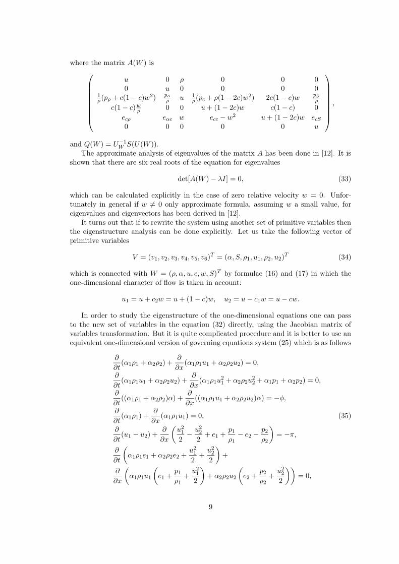
where the matrix A(W ) is
u 0 ρ 0 0 00 u 0 0 0 0
1ρ(pρ + c(1 − c)w2) pα
ρ u 1ρ(pc + ρ(1 − 2c)w2) 2c(1 − c)w pS
ρ
c(1 − c)wρ 0 0 u + (1 − 2c)w c(1 − c) 0
ecρ eαc w ecc − w2 u + (1 − 2c)w ecS
0 0 0 0 0 u
,
and Q(W ) = U−1W S(U(W )).
The approximate analysis of eigenvalues of the matrix A has been done in [12]. It isshown that there are six real roots of the equation for eigenvalues
det[A(W ) − λI] = 0, (33)
which can be calculated explicitly in the case of zero relative velocity w = 0. Unfor-tunately in general if w 6= 0 only approximate formula, assuming w a small value, foreigenvalues and eigenvectors has been derived in [12].
It turns out that if to rewrite the system using another set of primitive variables thenthe eigenstructure analysis can be done explicitly. Let us take the following vector ofprimitive variables
V = (v1, v2, v3, v4, v5, v6)T = (α, S, ρ1, u1, ρ2, u2)
T (34)
which is connected with W = (ρ, α, u, c, w, S)T by formulae (16) and (17) in which theone-dimensional character of flow is taken in account:
u1 = u + c2w = u + (1 − c)w, u2 = u − c1w = u − cw.
In order to study the eigenstructure of the one-dimensional equations one can passto the new set of variables in the equation (32) directly, using the Jacobian matrix ofvariables transformation. But it is quite complicated procedure and it is better to use anequivalent one-dimensional version of governing equations system (25) which is as follows
∂
∂t(α1ρ1 + α2ρ2) +
∂
∂x(α1ρ1u1 + α2ρ2u2) = 0,
∂
∂t(α1ρ1u1 + α2ρ2u2) +
∂
∂x(α1ρ1u
21 + α2ρ2u
22 + α1p1 + α2p2) = 0,
∂
∂t((α1ρ1 + α2ρ2)α) +
∂
∂x((α1ρ1u1 + α2ρ2u2)α) = −φ,
∂
∂t(α1ρ1) +
∂
∂x(α1ρ1u1) = 0, (35)
∂
∂t(u1 − u2) +
∂
∂x
(
u21
2−
u22
2+ e1 +
p1
ρ1− e2 −
p2
ρ2
)
= −π,
∂
∂t
(
α1ρ1e1 + α2ρ2e2 +u2
1
2+
u22
2
)
+
∂
∂x
(
α1ρ1u1
(
e1 +p1
ρ1+
u21
2
)
+ α2ρ2u2
(
e2 +p2
ρ2+
u22
2
))
= 0,
9
where the source terms are
φ =1
τ(p2 − p1), π = κc(1 − c)(u1 − u2).
The entropy balance law in the one-dimensional case becomes
∂
∂t((α1ρ1 + α2ρ2)S) +
∂
∂x((α1ρ1u1 + α2ρ2u2)S) = Q,
where the entropy production is
Q =1
eS
(
(p1 − p2)2
ρτ+ ρκc2(1 − c)2(u1 − u2)
2
)
≥ 0.
Further transformation of equations in order to simplify them and write them in aquasilinear form leads us to the following system:
∂α
∂t+ u
∂α
∂x= −
φ
ρ,
∂S
∂t+ u
∂S
∂x=
Q
ρ,
∂ρ1
∂t+ u1
∂ρ1
∂x+ ρ1
∂u1
∂x+
α2
α1
ρ1ρ2
ρ(u1 − u2)
∂α
∂x=
ρ1φ
α1ρ,
∂u1
∂t+ u1
∂u1
∂x+
1
ρ1
∂p1
∂x+
p1 − p2
ρ
∂α
∂x+
α2ρ2
ρ(T1 − T2)
∂S
∂x= −
α2ρ2
ρπ,
∂ρ2
∂t+ u2
∂ρ2
∂x+ ρ2
∂u2
∂x+
α1
α2
ρ1ρ2
ρ(u1 − u2)
∂α
∂x= −
ρ2φ
α2ρ,
∂u2
∂t+ u2
∂u2
∂x+
1
ρ2
∂p2
∂x+
p1 − p2
ρ
∂α
∂x−
α1ρ1
ρ(T1 − T2)
∂S
∂x=
α1ρ1
ρπ.
Here ρ = α1ρ1 + α2ρ2 and Ti = ∂ei/∂S. Certainly we assume αi 6= 0 and αi 6= 1Now it is not difficult to rewrite the latter system in quasilinear form in terms of the
set of primitive variables (34)
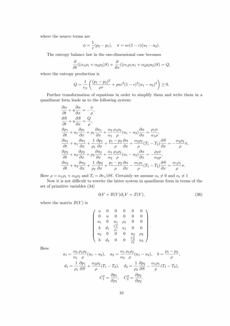
∂tV + B(V )∂xV = Z(V ), (36)
where the matrix B(V ) is
u 0 0 0 0 00 u 0 0 0 0a1 0 u1 ρ1 0 0
b d1C2
1
ρ1u1 0 0
a2 0 0 0 u2 ρ2
b d2 0 0C2
2
ρ2u2
.
Here
a1 =α2
α1
ρ1ρ2
ρ(u1 − u2), a2 =
α1
α2
ρ1ρ2
ρ(u1 − u2), b =
p1 − p2
ρ,
d1 =1
ρ1
∂p1
∂S+
α2ρ2
ρ(T1 − T2), d2 =
1
ρ2
∂p2
∂S−
α1ρ1
ρ(T1 − T2),
C21 =
∂p1
∂ρ1, C2
2 =∂p2
∂ρ2.
10
3.3 Eigenstructure and characteristic fields
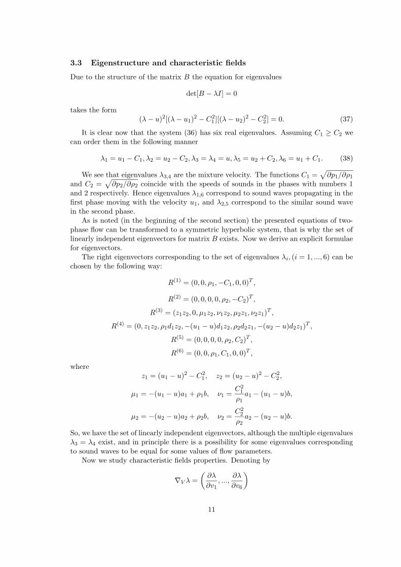
Due to the structure of the matrix B the equation for eigenvalues
det[B − λI] = 0
takes the form(λ − u)2[(λ − u1)
2 − C21 ][(λ − u2)
2 − C22 ] = 0. (37)
It is clear now that the system (36) has six real eigenvalues. Assuming C1 ≥ C2 wecan order them in the following manner
λ1 = u1 − C1, λ2 = u2 − C2, λ3 = λ4 = u, λ5 = u2 + C2, λ6 = u1 + C1. (38)
We see that eigenvalues λ3,4 are the mixture velocity. The functions C1 =√
∂p1/∂ρ1
and C2 =√
∂p2/∂ρ2 coincide with the speeds of sounds in the phases with numbers 1and 2 respectively. Hence eigenvalues λ1,6 correspond to sound waves propagating in thefirst phase moving with the velocity u1, and λ2,5 correspond to the similar sound wavein the second phase.
As is noted (in the beginning of the second section) the presented equations of two-phase flow can be transformed to a symmetric hyperbolic system, that is why the set oflinearly independent eigenvectors for matrix B exists. Now we derive an explicit formulaefor eigenvectors.
The right eigenvectors corresponding to the set of eigenvalues λi, (i = 1, ..., 6) can bechosen by the following way:
R(1) = (0, 0, ρ1,−C1, 0, 0)T ,
R(2) = (0, 0, 0, 0, ρ2,−C2)T ,
R(3) = (z1z2, 0, µ1z2, ν1z2, µ2z1, ν2z1)T ,
R(4) = (0, z1z2, ρ1d1z2,−(u1 − u)d1z2, ρ2d2z1,−(u2 − u)d2z1)T ,
R(5) = (0, 0, 0, 0, ρ2, C2)T ,
R(6) = (0, 0, ρ1, C1, 0, 0)T ,
wherez1 = (u1 − u)2 − C2
1 , z2 = (u2 − u)2 − C22 ,
µ1 = −(u1 − u)a1 + ρ1b, ν1 =C2
1
ρ1a1 − (u1 − u)b,
µ2 = −(u2 − u)a2 + ρ2b, ν2 =C2
2
ρ2a2 − (u2 − u)b.
So, we have the set of linearly independent eigenvectors, although the multiple eigenvaluesλ3 = λ4 exist, and in principle there is a possibility for some eigenvalues correspondingto sound waves to be equal for some values of flow parameters.
Now we study characteristic fields properties. Denoting by
∇V λ =
(
∂λ
∂v1, ...,
∂λ
∂v6
)
11
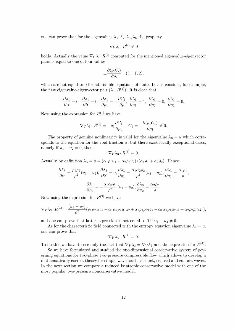
one can prove that for the eigenvalues λ1, λ2, λ5, λ6 the property
∇V λi · R(i) 6= 0
holds. Actually the value ∇V λi ·R(i) computed for the mentioned eigenvalue-eigenvector
pairs is equal to one of four values
±∂(ρiCi)
∂ρi(i = 1, 2),
which are not equal to 0 for admissible equations of state. Let us consider, for example,the first eigenvalue-eigenvector pair (λ1, R
(1)). It is clear that
∂λ1
∂α= 0,
∂λ1
∂S= 0,
∂λ1
∂ρ1= −
∂C1
∂ρ,
∂λ1
∂u1= 1,
∂λ1
∂ρ2= 0,
∂λ1
∂u2= 0.
Now using the expression for R(1) we have
∇V λ1 · R(1) = −ρ1
∂C1
∂ρ1− C1 = −
∂(ρ1C1)
∂ρ16= 0.
The property of genuine nonlinearity is valid for the eigenvalue λ3 = u which corre-sponds to the equation for the void fraction α, but there exist locally exceptional cases,namely if u1 − u2 = 0, then
∇V λ3 · R(3) = 0.
Actually by definition λ3 = u = (α1ρ1u1 + α2ρ2u2)/(α1ρ1 + α2ρ2). Hence
∂λ3
∂α=
ρ1ρ2
ρ2(u1 − u2),
∂λ3
∂S= 0,
∂λ3
∂ρ1=
α1α2ρ2
ρ2(u1 − u2),
∂λ3
∂u1=
α1ρ1
ρ,
∂λ3
∂ρ2= −
α1α2ρ1
ρ2(u1 − u2),
∂λ3
∂u2=
α2ρ2
ρ.
Now using the expression for R(3) we have
∇V λ3 ·R(3) =
(u1 − u2)
ρ2(ρ1ρ2z1z2 +α1α2ρ2µ1z2 +α1ρ1ρν1z2 −α1α2ρ1µ2z1 +α2ρ2ρν2z1),
and one can prove that latter expression is not equal to 0 if u1 − u2 6= 0.As for the characteristic field connected with the entropy equation eigenvalue λ4 = u,
one can prove that∇V λ4 · R
(4) ≡ 0.
To do this we have to use only the fact that ∇V λ3 = ∇V λ4 and the expression for R(4).So we have formulated and studied the one-dimensional conservative system of gov-
erning equations for two-phase two-pressure compressible flow which allows to develop amathematically correct theory for simple waves such as shock, centred and contact waves.In the next section we compare a reduced isentropic conservative model with one of themost popular two-pressure nonconservative model.
12
4 Comparison of models
In this paper we deal with conservative model of two-phase compressible flow with twovelocities and two pressures. In recent years the most established approach for modellingtwo-phase two-pressure compressible flows has been proposed in [1]. The approach con-sists of representation two-phase flow as two separate continua coupled by momentumand energy exchange. The resulting system of governing equations is hyperbolic but itis not in a conservative form. Several modifications of this approach [2],[4],[3],[?] hasbeen done. Models based on this approach we call Baer-Nunziato (BN) -type models.In this section we compare the governing equations discussed in previous sections withthe governing equations of the BN-type model. As was noted in the Section 2 our con-servative model is designed for processes in which the thermal state of phases is almostin equilibrium state, while BN-type models can take into account significant thermalnon-equilibrium. That is why it is reasonable to compare the reduced conservative andBN models in which thermal processes are ignored and the phases behavior is isentropic.
In this section we will show that the one-dimensional versions of the models aresimilar, that is to say, they can be written by the selfsame way formally. But there isa difference in the definition of interfacial pressure and certainly this difference can givedifferent results in the modelling of some phenomena. The models differ much more inthe multidimensional case: the conservative model contain lift forces [15] in the individualphase momentum equations which arise intrinsically due to the structure of conservativegoverning equations. The BN-type models do not contain terms corresponding to liftforces.
The general BN-type model consists of partial differential balance equations for mass,momentum, and energy for each of two phases completed by the evolution equation for thevolume fraction. Further we consider a simplified BN model in which thermal processesare ignored and hence the energy balance equations for each phase can be neglected. Thereduced isentropic model is governed by the five equations system
∂α1
∂t+ (uI)k
∂α1
∂xk= µ(p1 − p2),
∂α1ρ1
∂t+
∂α1ρ1(u1)k
∂xk= 0,
∂α1ρ1(u1)i
∂t+
∂α1ρ1(u1)i(u1)k
∂xk+
∂α1p1
∂xi= pI
∂α1
∂xi+ λ((u2)i − (u1)i), (39)
∂α2ρ2
∂t+
∂α2ρ2(u2)k
∂xk= 0,
∂α2ρ2(u2)i
∂t+
∂α2ρ2(u2)i(u2)k
∂xk+
∂α2p2
∂xi= pI
∂α2
∂xi− λ((u2)i − (u1)i).
Here, as in the previous sections, αi are the volume concentrations of phases (α1+α2 = 1),ρi are the mass densities, (ui)k are the k-th component of the velocity of i-th phase,|ui|
2 = (ui)21 + (ui)
22 + (ui)
23, pi is the pressure of i-th phase. The quantities (uI)k and pI
are called interfacial velocity and interfacial pressure respectively. They are determinedby the same way as average velocity and average pressure for the conservative model inprevious sections:
(uI)k = (u)k =α1ρ1(u1)k + α2ρ2(u2)k
α1ρ1 + α2ρ2, pI = p = α1p1 + α2p2.
13
Here we assume that for each phase its pressure is a known function of its density
pi = pi(ρi), (i = 1, 2).
It is interesting to compare also the one-dimensional versions of the conservative andBN-type models. Assuming that the mixture flows in the x = x1 direction and velocitiesu1 and u2 only exist, the one-dimensional version of BN equations is as follows
∂α1
∂t+ uI
∂α1
∂x= µ(p1 − p2),
∂α1ρ1
∂t+
∂α1ρ1u1
∂x= 0,
∂α1ρ1u1
∂t+
∂α1ρ1u21
∂x+
∂α1p1
∂x= pI
∂α1
∂x+ λ(u2 − u1), (40)
∂α2ρ2
∂t+
∂α2ρ2u2
∂x= 0,
∂α2ρ2u2
∂t+
∂α2ρ2u22
∂xk+
∂α2p2
∂x= pI
∂α2
∂x− λ(u2 − u1).
First of all we compare one-dimensional versions of conservative model from Section3 and the BN-type equations (40). Here we also consider a reduced conservative modelin which thermal processes are neglected. Such a modification of the system (35) is asfollows
∂
∂t(α1ρ1 + α2ρ2) +
∂
∂x(α1ρ1u1 + α2ρ2u2) = 0,
∂
∂t(α1ρ1u1 + α2ρ2u2) +
∂
∂x(α1ρ1u
21 + α2ρ2u
22 + α1p1 + α2p2) = 0,
∂
∂t((α1ρ1 + α2ρ2)α) +
∂
∂x((α1ρ1u1 + α2ρ2u2)α) = −φ, (41)
∂
∂t(α1ρ1) +
∂
∂x(α1ρ1u1) = 0,
∂
∂t(u1 − u2) +
∂
∂x
(
u21
2−
u22
2+ e1 +
p1
ρ1− e2 −
p2
ρ2
)
= −π.
It is obvious that using the first and third equations of the system (41) one can derivethe evolution equation for the volume fraction α = α1 in the form
∂α
∂t+ u
∂α
∂x= −φ, (42)
It is also clear that from the first and fourth equations of the system (41) the massconservation equation for the second phase follows
∂
∂t(α2ρ2) +
∂
∂x(α2ρ2u2) = 0. (43)
And finally, after some cumbersome transformation, using the second (total momen-tum) and fifth (relative velocity) equations of the system (41), one can derive the mo-mentum balance equations for each phase:
∂α1ρ1u1
∂t+
∂α1ρ1u21
∂x+
∂α1p1
∂x=
α2ρ2p1 + α1ρ1p2
ρ
∂α1
∂x−
α1α2ρ1ρ2
ρπ, (44)
∂α2ρ2u2
∂t+
∂α2ρ2u22
∂xk+
∂α2p2
∂x=
α2ρ2p1 + α1ρ1p2
ρ
∂α2
∂x+
α1α2ρ1ρ2
ρπ. (45)
14
So, combining equations (42)-(45) and the fourth equation of the system (41) weobtain the complete one-dimensional system for isentropic two-phase flow
∂α
∂t+ uI
∂α
∂x= −φ,
∂
∂t(α1ρ1) +
∂
∂x(α1ρ1u1) = 0,
∂
∂t(α2ρ2) +
∂
∂x(α2ρ2u2) = 0, (46)
∂α1ρ1u1
∂t+
∂α1ρ1u21
∂x+
∂α1p1
∂x= pI
∂α1
∂x−
α1α2ρ1ρ2
ρπ,
∂α2ρ2u2
∂t+
∂α2ρ2u22
∂xk+
∂α2p2
∂x= pI
∂α2
∂x+
α1α2ρ1ρ2
ρπ.
Recalling the definition of the source terms (see Section 3)
φ =1
τ(p2 − p1), π = κ
α1α2ρ1ρ2
ρ2(u1 − u2),
we conclude that the latter system is similar to the one-dimensional version of BN model(40) if to denote
µ = −1
τ, λ = −κ
(α1α2ρ1ρ2)2
ρ3.
The definition of interfacial velocity is the same for both models
uI = u =α1ρ1u1 + α2ρ2u2
α1ρ1 + α2ρ2,
but the definition of interfacial pressure is different. In the BN-type model we havepI = α1p1 + α2p2 while in the conservative model
pI =α2ρ2p1 + α1ρ1p2
α1ρ1 + α2ρ2.
Such a difference in definition of internal pressure in the BN model and conservativemodel can lead to a different behavior of solutions for concrete problems. Although inthe case of very fast pressure relaxation the solutions could be close because in this casethe phases pressures must be very close to a common uniform value.
The difference between two models becomes more significant in the multidimensionalcase. Now we will not present the complete comparison of governing equations for bothmodels. We note only that the mass conservation equations for each phase and relaxationequation for the volume fraction remain identical for both models. But in the phasemomentum balance equations derived from the present conservative model an additionalterms connected with phase vorticities arise.
Actually, from the total momentum equation (second equation in (25)) and the rel-ative velocity equation (fifth equation in (25)) for the mixture, after cumbersome trans-formations the equations for phases momentum follow
∂α1ρ1(u1)i
∂t+
∂α1ρ1(u1)i(u1)k
∂xk+
∂α1p1
∂xi= pI
∂α1
∂xi+ Fi −
α1α2ρ1ρ2
ρπ, (47)
∂α2ρ2(u2)i
∂t+
∂α2ρ2(u2)i(u2)k
∂xk+
∂α2p2
∂xi= pI
∂α2
∂xi− Fi +
α1α2ρ1ρ2
ρπ. (48)
15
We can see that in equations (47),(48) an additional extra terms Fi arise which are notpresented in the BN-type equations (39). These terms are defined as follows
Fi = ρc1c2((u1)k − (u2)k)
(
c1
(
∂(u2)i
∂xk−
∂(u2)k
∂xi
)
+ c2
(
∂(u1)i
∂xk−
∂(u1)k
∂xi
))
.
Here ci = (αiρi)/ρ, i = 1, 2 are the phase mass fractions.Terms Fi describe the forces arising for the flow with nonzero relative velocity and
caused by the phases vorticities. Such type of force is called as lift force, see for example[15].
So there is a difference between governing equations for isentropic processes in the BN-type model and conservative model. The distinctions appear in the phases momentumbalance equations. First distinction is in the definition of the interfacial pressure. Thesecond one appears in multidimensional case only, namely, the lift forces are presentedin the conservative model, but they are not presented in the BN-type model.
5 Numerical methods
Here we consider finite volume schemes for solving numerically the two-phase flow equa-tions studied in previous sections of this paper. We restrict the presentation to systemsof the form
∂tQ + ∂xF(Q) = S(Q) , (49)
where Q is the vector of conserved variables, F(Q) is the vector of fluxes and S(Q) isthe vector of sources, assumed to be a non-differential term, e.g. algebraic.
Finite volume schemes for solving (49) numerically are constructed by first integrating(49) over a control volume V ≡ [xi− 1
2
, xi+ 1
2
] × [tn, tn+1] of dimensions
∆x = xi+ 1
2
− xi− 1
2
, ∆t = tn+1 − tn . (50)
The result is the exact relation
Qn+1i = Qn
i −∆t
∆x
[
Fi+1/2 − Fi−1/2
]
+ ∆tSi , (51)
where
Qni =
1
∆x
∫ xi+1/2
xi−1/2
Q(x, tn) dx ,
Fi+1/2 =1
∆t
∫ tn+1
tnF(Q(xi+1/2, τ)) dτ ,
Si =1
∆t
1
∆x
∫ tn+1
tn
∫ xi+1/2
xi−1/2
S(Q(x, τ)) dx dτ .
(52)
Conservative numerical schemes may be constructed from the exact relation (51)-(52)by defining suitable approximations to (52) leading to numerical fluxes and numericalsources, still denoted by the symbols Fi+1/2 and Si respectively.
16
Here we consider centred, as distinct from upwind, schemes. The most well-knowncentred schemes is that given by the Lax-Friedrichs numerical flux, namely
FLFi+1/2 =
1
2
[
F(Qni ) + F(Qn
i+1)]
−∆x
∆t
[
Qni+1 − Qn
i
]
. (53)
The conservative scheme (51) along with the numerical flux (53) gives the Lax-Friedrichsscheme, which is first-order accurate, mononote and stable to CFL unity, where CFL isthe maximum Courant, or CFL, number. This scheme is very simple but is the mostdiffusive of all stable three-point schemes and thus is not recommended for practical use.
An improvement is obtained by using the FORCE flux [16]- [18]
FFORCEi+1/2 = 1
4 [F(Qni ) + 2F(Q
n+ 1
2
i+ 1
2
) + F(Qni+1) −
∆x∆t (Q
ni+1 − Qn
i )],
Qn+ 1
2
i+ 1
2
= 12 [Qn
i + Qni+1] −
12
∆t∆x [F(Qn
i+1) − F(Qni )].
This numerical flux leads to a conservative scheme that is first-order accurate, monotoneand more accurate than that of Lax-Friedrichs. Recently, the scheme has been proved tobe convergent, for a 2 × 2 system of non-linear conservation laws [19].
A second-order non-oscillatory (TVD) extension of the FORCE flux is the SLICscheme [18], which is based on MUSCL linear reconstructions in each cell i, leading totwo boundary extrapolated values
QLi = Qn
i −1
2∆i , QR
i = Qni +
1
2∆i ,
where ∆i = φ∆i is a TVD limited slope (actually a vector difference), φ is a slope limiterfunction and ∆i is a slope of the form
∆i = ω∆i− 1
2
+ (1 − ω)∆i+ 1
2
, ∆i+ 1
2
= Qni+1 − Qn
i
with ω a parameter in the real interval [0, 1]. One usually takes ω = 0.In the scheme, the boundary extrapolated values are then evolved in time by half a
time step as follows:
QLi = QL
i −1
2
∆t
∆x[F(QR
i ) − F(QLi )] , QR
i = QRi −
1
2
∆t
∆x[F(QR
i ) − F(QLi )] .
In the final step of the scheme we evaluate the FORCE flux FFORCEi+1/2 (A,B) with argu-
ments A = QRi and B = QL
i+1.The resulting scheme is the second-order non-oscillatory SLIC scheme, which is simple
and easily applicable to complex non-linear systems, such as those studied in this paper.Full details SLIC scheme are found in [17]. Regarding the source terms, there are variousapproaches that can be used. For details see Chapter 15 of [17].
6 Numerical Examples
In this section we study two test problems numerically using the reduced isentropic ver-sion of the conservative model for two-phase flow. The governing equations are taken
17

in the form (41) neglecting the interfacial interactions, namely pressure relaxation andinterfacial friction. Obviously such a simplified system will not accurately describe phe-nomena involving strong shock waves but will still be useful for a valuable range ofproblems. Moreover, for this model it is easy to analyse the mathematical characterof the system and to test new idea regarding numerical methods for multiphase flowproblems. For the source terms we assume φ = 0 and π = 0.
Each of the test problems represents a Riemann problem for an air/water mixture.Suppose that index 1 denotes the air parameters and index 2 denotes the water param-eters. The closing constitutive relationships which are needed to close the model are theisentropic equations of state relating pressures to densities. For air, the isentropic perfectgas law is
p1 = A1
(
ρ1
ρ01
)γ1
, (54)
with constants ρ01 = 1kg/m3, A1 = 105Pa, γ = 1.4.
For water we take the Tait’s equation of state
p2 = A2
(
ρ2
ρ02
)γ2
− A3, (55)
with ρ02 = 103kg/m3, A2 = 8.5 × 10⁸Pa, A3 = 8.4999 × 10⁸Pa, γ2 = 2.8.
For the initial conditions in both test problems we assume that the mixture hasconstant volume fractions of air and water of 0.9 and 0.1 respectively and that thepressure of air and water in the initial data are equal and it is a given value. The valuesof phase densities in the initial data can be evaluated by formulae (54) and (55).
For both test problems the computational domain is the real interval [0, 1]. In eachtest the initial data defines a Riemann problem with a left section [0, 1/2) and a rightsection [1/2, 1].
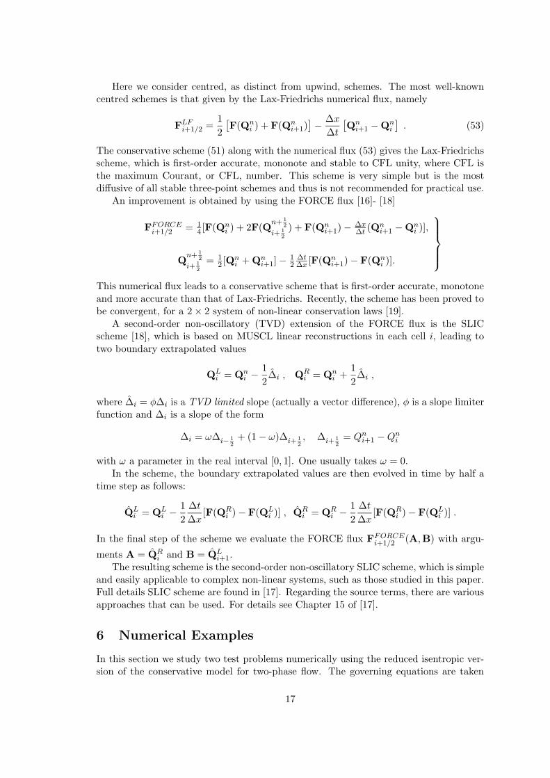
6.1 Test 1: Symmetric four-rarefaction problem
This test problem has initial data:Left section: p = 109Pa, u1 = u2 = −1.8 × 10³m/s,Right section: p = 109Pa, u1 = u2 = 1.8 × 10³m/s.
Figs. 1 to 4 show computed results at time 0.11 × 10⁻⁵s, using various meshes, forliquid and gas densities, liquid and gas velocities, mixture density and pressure, mixturevelocity and relative velocity. The CFL coefficient used in the calculations was CFL= 0.9.
Fig. 1 shows a reference numerical solution computed with a fine mesh of 4000 cellsand the best of the numerical methods presented in this paper, namely SLIC, whichis a second-order TVD method. The structure of the solution contains four symmetricrarefaction waves, two for each phase. The solution also contains a middle region in whichthe density of both phases is very low. In fact this is the main feature that motivatesthe choice of this test problem for assessing numerical methods. For single-phase flow,it is a well documented fact that the computation of low density flows is indeed verychallenging; it is known that all linearized Riemann solvers, for example, will lead to thecomputation of negative densities [20].
The four-rarefaction structure becomes more complex when we examine the mixturequantities. Due to the superposition of the two waves for each of the two phases we endup with a structure that contains, apparently, six waves. See for example the mixture
18
density and the relative velocity. The computed results of Fig. 1 look very satisfactoryin that all the expected features of the solution are well resolved. We note, however, thatthere is a small spurious overshoot in the solution; this is more evident in the relativevelocity profile.
Figs. 2 to 4 show numerical results for a coarse mesh of 100 cells (thin line) comparedwith the reference solution (thick line), for three schemes, namely Lax-Friedrichs, FORCEand SLIC. It is obvious that the Lax-Friedrichs scheme is too inaccurate to be used inpractice. As judging from the results of these figures, the best scheme is the second-orderTVD method, SLIC.
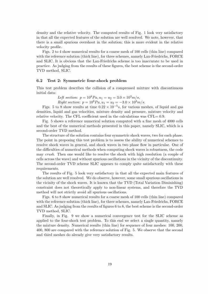
6.2 Test 2: Symmetric four-shock problem
This test problem describes the collision of a compressed mixture with discontinuousinitial data:
Left section: p = 108Pa, u1 = u2 = 3.0 × 10³m/s,Right section: p = 108Pa, u1 = u2 = −3.0 × 10³m/s.
Figs. 5 to 8 show results at time 0.22 × 10⁻⁵s, for various meshes, of liquid and gasdensities, liquid and gas velocities, mixture density and pressure, mixture velocity andrelative velocity. The CFL coefficient used in the calculations was CFL= 0.9.
Fig. 5 shows a reference numerical solution computed with a fine mesh of 4000 cellsand the best of the numerical methods presented in this paper, namely SLIC, which is asecond-order TVD method.
The structure of the solution contains four symmetric shock waves, two for each phase.The point in proposing this test problem is to assess the ability of numerical schemes toresolve shock waves in general, and shock waves in two phase flow in particular. One ofthe difficulties of numerical methods when computing shock waves is robustness, the codemay crush. Then one would like to resolve the shock with high resolution (a couple ofcells across the wave) and without spurious oscillations in the vicinity of the discontinuity.The second-order TVD scheme SLIC appears to comply quite satisfactorily with theserequirements.
The results of Fig. 5 look very satisfactory in that all the expected main features ofthe solution are well resolved. We do observe, however, some small spurious oscillations inthe vicinity of the shock waves. It is known that the TVD (Total Variation Diminishing)constraint does not theoretically apply to non-linear systems, and therefore the TVDmethod will not strictly avoid all spurious oscillations.
Figs. 6 to 8 show numerical results for a coarse mesh of 100 cells (thin line) comparedwith the reference solution (thick line), for three schemes, namely Lax-Friedrichs, FORCEand SLIC. As judging from the results of figures 6 to 8, the best scheme is the second-orderTVD method, SLIC.
Finally, in Fig. 9 we show a numerical convergence test for the SLIC scheme asapplied to the four-shock test problem. To this end we select a single quantity, namelythe mixture density. Numerical results (thin line) for sequence of four meshes: 100, 200,400, 800 are compared with the reference solution of Fig. 5. We observe that the secondand third meshes do already give very satisfactory results.
19
7 Conclusions
The governing equations of a conservative two-phase two-pressure model based on ex-tended thermodynamics principles are studied. The system is hyperbolic and is writtenin conservation-law form. In the one-dimensional case the system has six equations, forwhich the full eigenstructure analysis is performed, namely, explicit formulae for eigenval-ues and eigenvectors are derived and the corresponding characteristic fields are studied.
The reduced isentropic conservative system is formulated and compared with the cor-responding isentropic Baer-Nunziato-type model. It is shown that the one-dimensionalversion of the present conservative system is similar to the Baer-Nunziato-type modelexcept for the definition of interfacial pressure, which is included into the differentialsource terms in the momentum equations. Moreover, it turns out that for the multidi-mensional case the lift forces included in the momentum equations of the present modeldo not appear in the Baer-Nunziato-type model.
Conservative shock-capturing of the centred type are then proposed to solve thegoverning equations. Test problems are proposed and numerical results are shown anddiscussed.
Acknowledgements
The paper is based on research partially performed during the participation of the authorsin the programme Nonlinear Hyperbolic Waves in Phase Dynamics and Astrophysics atthe Isaac Newton Institute for Mathematical Sciences, University of Cambridge. Thesecond author acknowledges the support provided by the Isaac Newton Institute forMathematical Sciences, University of Cambridge, UK, as co-organizer of the six-monthsprogramme on Nonlinear Hyperbolic Waves in Phase Dynamics and Astrophysics, Jan-uary to July 2003, and the associated EPSRC senior visiting fellowship, grant GR N09276.The first author acknowledges the Italian Ministry of Education and Research (MIUR)for the financial support provided during his stay as visiting professor at the Departmentof Civil and Environmental Engineering, University of Trento.
References
[1] Baer, M., Nunziato, J.: A two-phase mixture theory for the deflagration-to-detonationtransition (DDT) in reactive granular materials. Int. J. Multiphase Flow 12, 861–889(1986)
[2] Bdzil, J., Menikoff, R., Son, S., Kapila, A., Stewart, D.: Two-phase modeling ofdeflagration-to-detonation transition in granular materials: a critical examination ofmodeling issues. Physics of Fluids 11, 378–402 (1999)
[3] Saurel, R., Abgrall, R.: A multiphase Godunov method for compressible multifluidand multiphase flows. J. Comput. Phys. 150 425–467 (1999)
[4] Gavrilyuk, S., Saurel, R.: Mathematical and numerical modeling of two-phase com-pressible flows with micro-inertia. J. Comput. Phys. 175, 326–360 (2002)
20
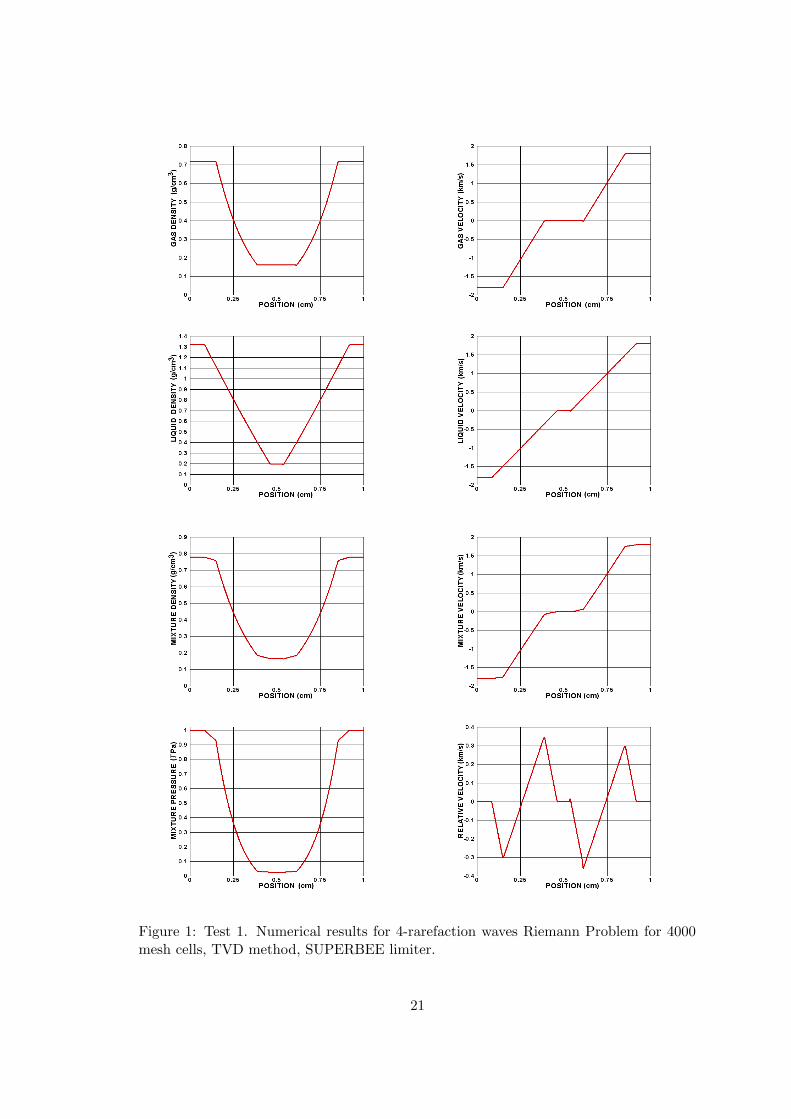
Figure 1: Test 1. Numerical results for 4-rarefaction waves Riemann Problem for 4000mesh cells, TVD method, SUPERBEE limiter.
21
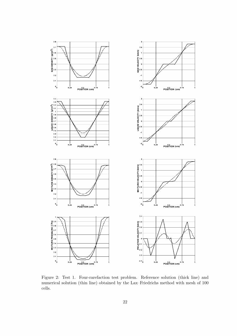
Figure 2: Test 1. Four-rarefaction test problem. Reference solution (thick line) andnumerical solution (thin line) obtained by the Lax–Friedrichs method with mesh of 100cells.
22
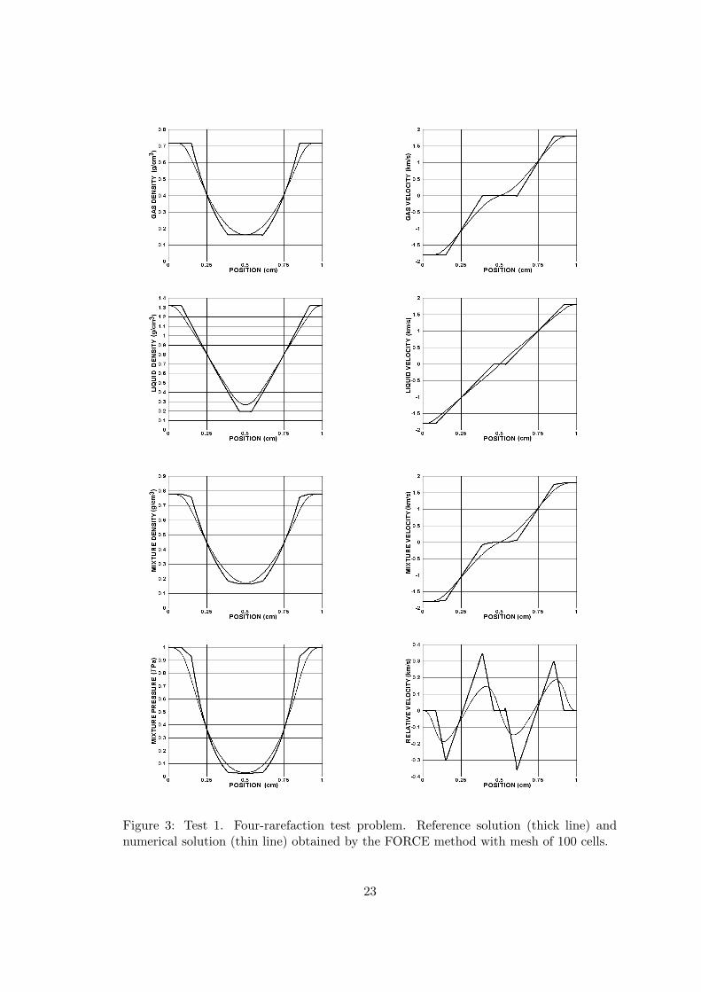
Figure 3: Test 1. Four-rarefaction test problem. Reference solution (thick line) andnumerical solution (thin line) obtained by the FORCE method with mesh of 100 cells.
23
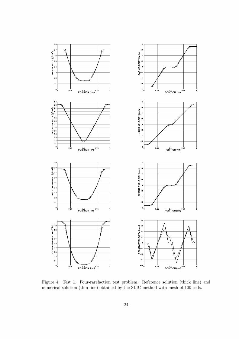
Figure 4: Test 1. Four-rarefaction test problem. Reference solution (thick line) andnumerical solution (thin line) obtained by the SLIC method with mesh of 100 cells.
24
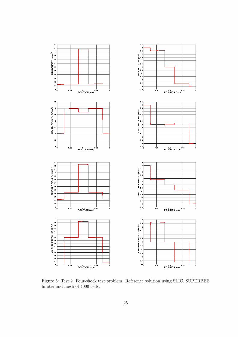
Figure 5: Test 2. Four-shock test problem. Reference solution using SLIC, SUPERBEElimiter and mesh of 4000 cells.
25
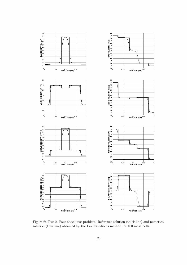
Figure 6: Test 2. Four-shock test problem. Reference solution (thick line) and numericalsolution (thin line) obtained by the Lax–Friedrichs method for 100 mesh cells.
26
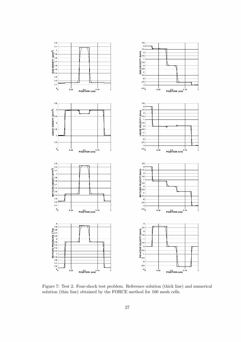
Figure 7: Test 2. Four-shock test problem. Reference solution (thick line) and numericalsolution (thin line) obtained by the FORCE method for 100 mesh cells.
27
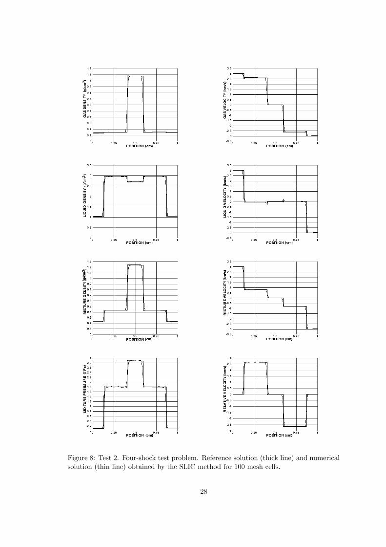
Figure 8: Test 2. Four-shock test problem. Reference solution (thick line) and numericalsolution (thin line) obtained by the SLIC method for 100 mesh cells.
28
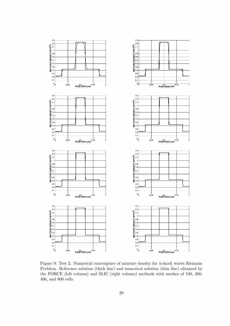
Figure 9: Test 2. Numerical convergence of mixture density for 4-shock waves RiemannProblem. Reference solution (thick line) and numerical solution (thin line) obtained bythe FORCE (left column) and SLIC (right column) methods with meshes of 100, 200,400, and 800 cells.
29
[5] Serre, D.: Sur le principe variationnel des equations de la mecanique des fluidesparfaits. Model Math. Anal. Numer. 27 739–758 (1993)
[6] Gouin, H., Gavrilyuk, S.: Hamilton’s Principle and Rankine–Hugoniot Conditions forGeneral Motions of Mixtures. Meccanica 34 39–47 (1999)
[7] Godunov, S., Romensky, E.: Thermodynamics, conservation laws and symmetricforms of differential equations in mechanics of continuous media. In Computational
Fluid Dynamics Review 1995, John Wiley & Sons, New York, 19–31 (1995)
[8] Romensky, E.: Hyperbolic systems of thermodynamically compatible conservationlaws in continuum mechanics. Math. Comput. Modelling 28, 115–130 (1998)
[9] Godunov, S.K., Romenski, E.: Elements of continuum mechanics and conservation
laws Kluwer Academic/Plenum Publishers, New York (2003)
[10] Muller, I., Ruggeri, T.: Rational extended thermodynamics Springer-Verlag, NewYork (1998)
[11] Romensky, E.: Thermodynamics and hyperbolic systems of balance laws in con-tinuum mechanics. In Godunov Methods: theory and applications, E. F. Toro (ed.),Kluwer Academic/Plenum publishers, 745–761 (2001)
[12] Romenski, E., Zeidan, D., Slaouti, A., Toro, E.F.: Hyperbolic conservative modelfor compressible two-phase flow. Isaac Newton Institute for Mathematical Sciences,Cambridge University, UK, Preprint NI03022-NPA (2003)
[13] Romenski, E., Toro, E.F.: Hyperbolicity and one-dimensional waves in compressibletwo-phase flow models. Shock Waves (accepted, available online)
[14] Resnyansky, A.D.: A thermodynamically complete model for simulation of one-dimensional multiphase flows. DSTO System Sciences Laboratory, Edinburgh SouthAustralia, Preprint DSTO-TR-1510 (2003)
[15] Drew, D.A., Lahey, R.T.Jr.: The virtual mass and lift force on a sphere in rotatingand straining inviscid flow. Int. J. Multiphase Flow 13, 113-121 (1987)
[16] Toro, E.F.: On Glimm-Related Schemes for Conservation Laws. Technical ReportMMU-9602, Department of Mathematics and Physics, Manchester Metropolitan Uni-versity, England. (1996)
[17] Toro, E.F.: Riemann Solvers and Numerical Methods for Fluid Dynamics, SecondEdition. Springer-Verlag. (1999)
[18] Toro, E.F., Billett, S.J.: Centred TVD Schemes for Hyperbolic Conservation Laws.IMA J. Numerical Analysis 20, 47–79 (2000)
[19] Chen, G.Q., Toro, E.F.: Centred Schemes for Non-Linear Hyperbolic Equations.Isaac Newton Institute for Mathematical Sciences, Cambridge University, UK, PreprintNI03046-NPA (2003)
[20] Einfeldt, B., Munz, C.D., Roe, P.L., Sjogreen, B.: On Godunov-Type Methods nearLow Densities. J. Comput. Phys. 92, 273–295 (1991)
30