Embed Size (px)
Citation preview

Aggregate Demand and Aggregate Supply Premium
PowerPoint Slides by
Ron Cronovich
© 2012 Cengage Learning. All Rights Reserved. May not be copied, scanned, or duplicated, in whole or in part, except for use as permitted in a license distributed with a certain product or service or otherwise on a password-protected website for classroom use.
N. Gregory Mankiw
Macroeconomics
Principles of
Sixth Edition
20
© 2012 Cengage Learning. All Rights Reserved. May not be copied, scanned, or duplicated, in whole or in part, except for use as permitted in a license distributed with a certain product or service or otherwise on a password-protected website for classroom use.
22
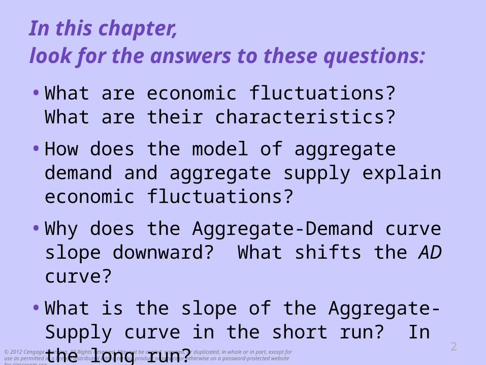
In this chapter, look for the answers to these questions:
• What are economic fluctuations? What are their characteristics?
• How does the model of aggregate demand and aggregate supply explain economic fluctuations?
• Why does the Aggregate-Demand curve slope downward? What shifts the AD curve?
• What is the slope of the Aggregate-Supply curve in the short run? In the long run? What shifts the AS curve(s)?
© 2012 Cengage Learning. All Rights Reserved. May not be copied, scanned, or duplicated, in whole or in part, except for use as permitted in a license distributed with a certain product or service or otherwise on a password-protected website for classroom use.
33
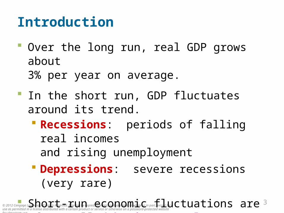
Introduction
Over the long run, real GDP grows about 3% per year on average.
In the short run, GDP fluctuates around its trend. Recessions: periods of falling real incomes
and rising unemployment Depressions: severe recessions (very rare)
Short-run economic fluctuations are often called business cycles.
1965 1970 1975 1980 1985 1990 1995 2000 2005 20100
2,000
4,000
6,000
8,000
10,000
12,000
14,000
16,000
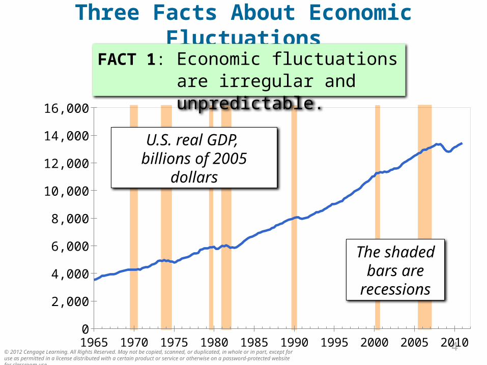
Three Facts About Economic Fluctuations
FACT 1: Economic fluctuations are irregular and unpredictable.
U.S. real GDP, billions of 2005 dollars
The shaded bars are
recessions
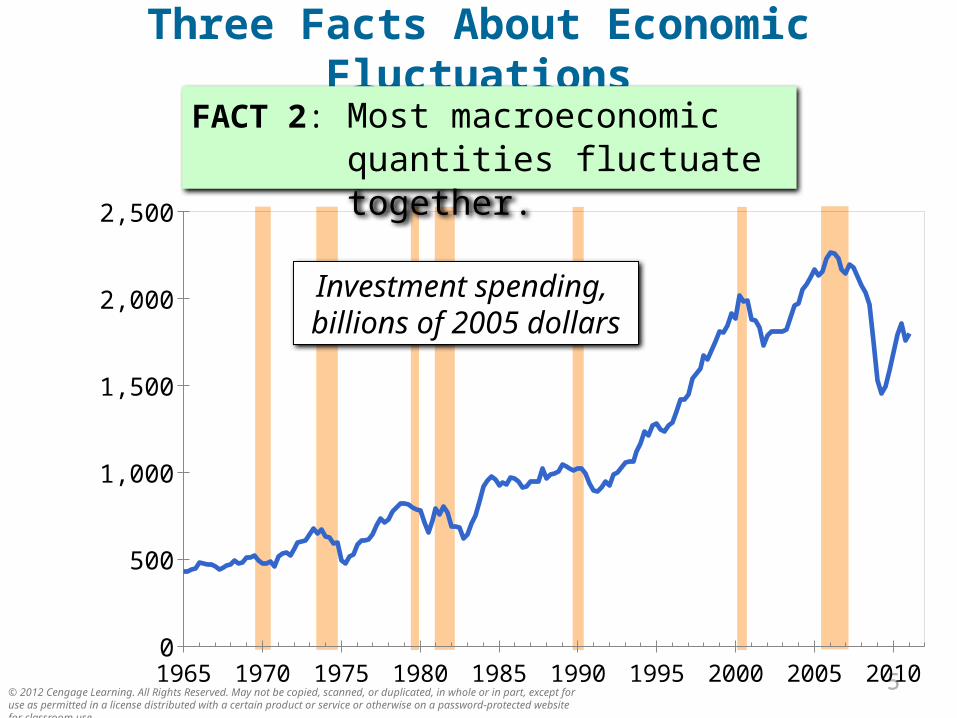
Three Facts About Economic Fluctuations
FACT 2: Most macroeconomic quantities fluctuate together.
1965 1970 1975 1980 1985 1990 1995 2000 2005 20100
500
1,000
1,500
2,000
2,500
Investment spending, billions of 2005 dollars
1965 1970 1975 1980 1985 1990 1995 2000 2005 20100
2
4
6
8
10
12
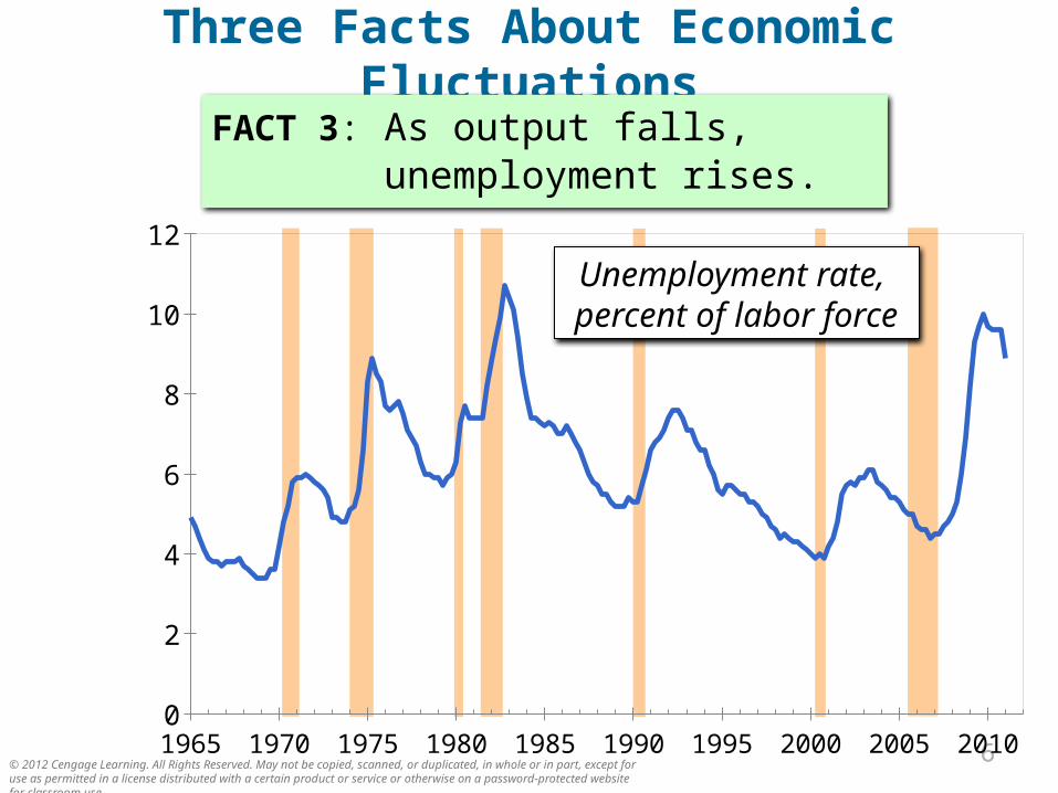
Three Facts About Economic Fluctuations
FACT 3: As output falls, unemployment rises.
Unemployment rate, percent of labor force
© 2012 Cengage Learning. All Rights Reserved. May not be copied, scanned, or duplicated, in whole or in part, except for use as permitted in a license distributed with a certain product or service or otherwise on a password-protected website for classroom use.
77
Introduction, continued
Explaining these fluctuations is difficult, and the theory of economic fluctuations is controversial.
Most economists use the model of aggregate demand and aggregate supply to study fluctuations.
This model differs from the classical economic theories economists use to explain the long run.
© 2012 Cengage Learning. All Rights Reserved. May not be copied, scanned, or duplicated, in whole or in part, except for use as permitted in a license distributed with a certain product or service or otherwise on a password-protected website for classroom use.
88
Classical Economics—A Recap
The previous chapters are based on the ideas of classical economics, especially:
The Classical Dichotomy, the separation of variables into two groups: Real – quantities, relative prices Nominal – measured in terms of money
The neutrality of money: Changes in the money supply affect nominal but not real variables.
© 2012 Cengage Learning. All Rights Reserved. May not be copied, scanned, or duplicated, in whole or in part, except for use as permitted in a license distributed with a certain product or service or otherwise on a password-protected website for classroom use.
99
Classical Economics—A Recap
Most economists believe classical theory describes the world in the long run, but not the short run.
In the short run, changes in nominal variables (like the money supply or P ) can affect real variables (like Y or the u-rate).
To study the short run, we use a new model.
© 2012 Cengage Learning. All Rights Reserved. May not be copied, scanned, or duplicated, in whole or in part, except for use as permitted in a license distributed with a certain product or service or otherwise on a password-protected website for classroom use.
1010
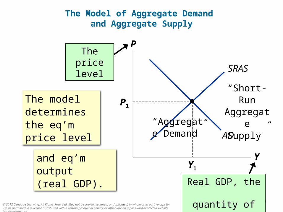
The Model of Aggregate Demand and Aggregate Supply
P
Y
AD
SRAS
P1
Y1
The price level
Real GDP, the quantity of output
The model determines the eq’m price level
and eq’m output (real GDP).
“Aggregate Demand”
“Short-Run Aggregate
Supply”
© 2012 Cengage Learning. All Rights Reserved. May not be copied, scanned, or duplicated, in whole or in part, except for use as permitted in a license distributed with a certain product or service or otherwise on a password-protected website for classroom use.
1111
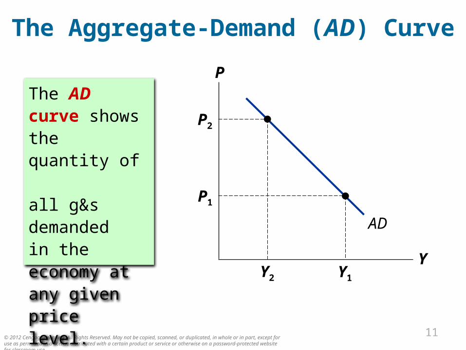
The Aggregate-Demand (AD) Curve
The AD curve shows the quantity of all g&s demanded in the economy at any given price level.
P
Y
AD
P1
Y1
P2
Y2
© 2012 Cengage Learning. All Rights Reserved. May not be copied, scanned, or duplicated, in whole or in part, except for use as permitted in a license distributed with a certain product or service or otherwise on a password-protected website for classroom use.
1212
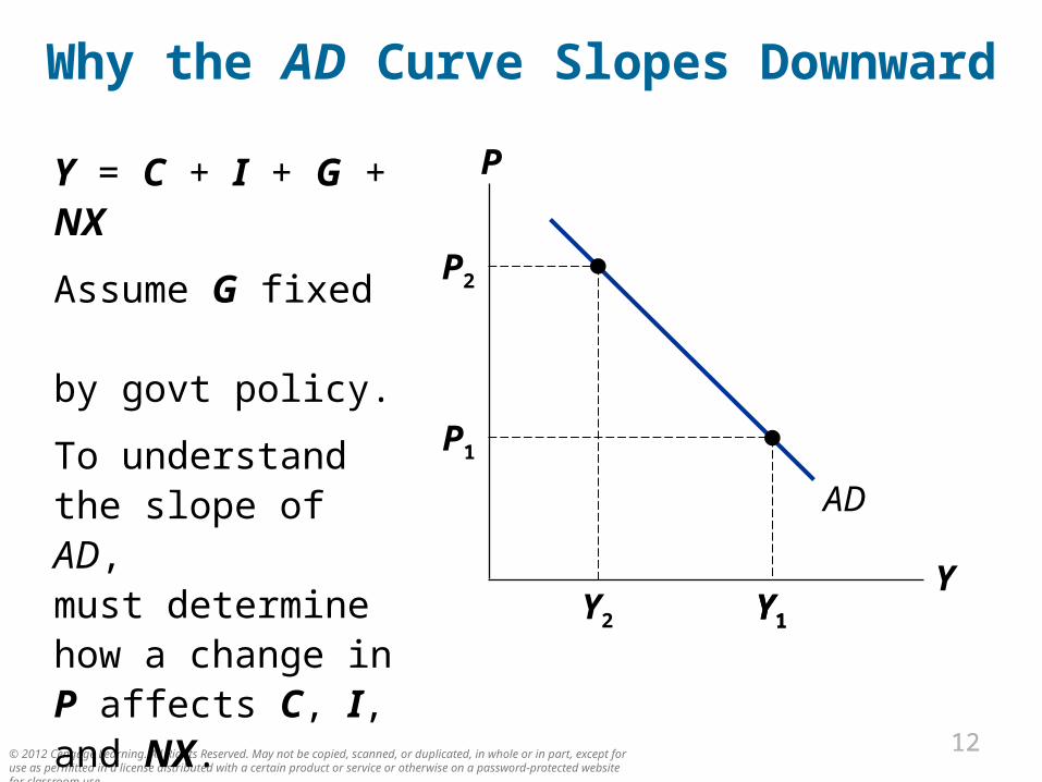
Why the AD Curve Slopes Downward
Y = C + I + G + NX
Assume G fixed by govt policy.
To understand the slope of AD, must determine how a change in P affects C, I, and NX.
P
Y
AD
P1
Y1
P2
Y2 Y1
© 2012 Cengage Learning. All Rights Reserved. May not be copied, scanned, or duplicated, in whole or in part, except for use as permitted in a license distributed with a certain product or service or otherwise on a password-protected website for classroom use.
1313
The Wealth Effect (P and C )
Suppose P rises.
The dollars people hold buy fewer g&s, so real wealth is lower.
People feel poorer.
Result: C falls.
© 2012 Cengage Learning. All Rights Reserved. May not be copied, scanned, or duplicated, in whole or in part, except for use as permitted in a license distributed with a certain product or service or otherwise on a password-protected website for classroom use.
1414
The Interest-Rate Effect (P and I )
Suppose P rises.
Buying g&s requires more dollars.
To get these dollars, people sell bonds or other assets.
This drives up interest rates.
Result: I falls.(Recall, I depends negatively on interest rates.)
© 2012 Cengage Learning. All Rights Reserved. May not be copied, scanned, or duplicated, in whole or in part, except for use as permitted in a license distributed with a certain product or service or otherwise on a password-protected website for classroom use.
1515
The Exchange-Rate Effect (P and NX )
Suppose P rises.
U.S. interest rates rise (the interest-rate effect).
Foreign investors desire more U.S. bonds.
Higher demand for $ in foreign exchange market.
U.S. exchange rate appreciates.
U.S. exports more expensive to people abroad, imports cheaper to U.S. residents.
Result: NX falls.
© 2012 Cengage Learning. All Rights Reserved. May not be copied, scanned, or duplicated, in whole or in part, except for use as permitted in a license distributed with a certain product or service or otherwise on a password-protected website for classroom use.
1616
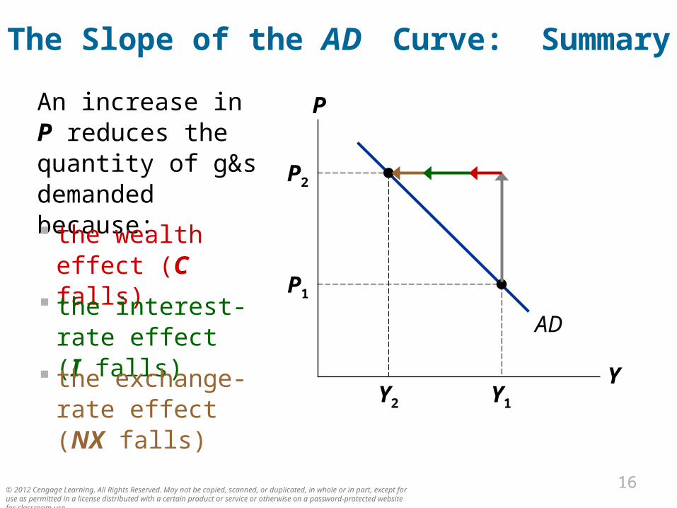
The Slope of the AD Curve: Summary
An increase in P reduces the quantity of g&s demanded because:
P
Y
AD
P1
Y1
the wealth effect (C falls)
P2
Y2
the interest-rate effect (I falls)
the exchange-rate effect (NX falls)
© 2012 Cengage Learning. All Rights Reserved. May not be copied, scanned, or duplicated, in whole or in part, except for use as permitted in a license distributed with a certain product or service or otherwise on a password-protected website for classroom use.
1717
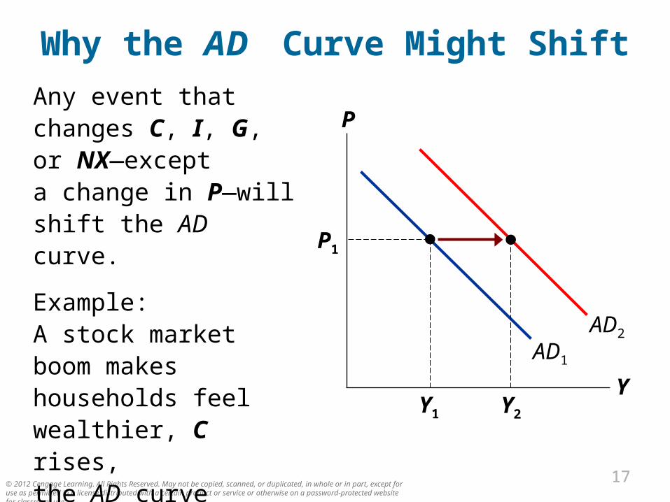
Why the AD Curve Might ShiftAny event that changes C, I, G, or NX—except a change in P—will shift the AD curve.
Example: A stock market boom makes households feel wealthier, C rises, the AD curve shifts right.
P
Y
AD1
AD2
Y2
P1
Y1
© 2012 Cengage Learning. All Rights Reserved. May not be copied, scanned, or duplicated, in whole or in part, except for use as permitted in a license distributed with a certain product or service or otherwise on a password-protected website for classroom use.
1818
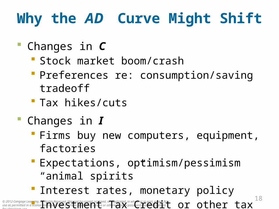
Why the AD Curve Might Shift
Changes in C Stock market boom/crash Preferences re: consumption/saving tradeoff Tax hikes/cuts
Changes in I Firms buy new computers, equipment, factories Expectations, optimism/pessimism “animal
spirits” Interest rates, monetary policy Investment Tax Credit or other tax incentives
© 2012 Cengage Learning. All Rights Reserved. May not be copied, scanned, or duplicated, in whole or in part, except for use as permitted in a license distributed with a certain product or service or otherwise on a password-protected website for classroom use.
1919
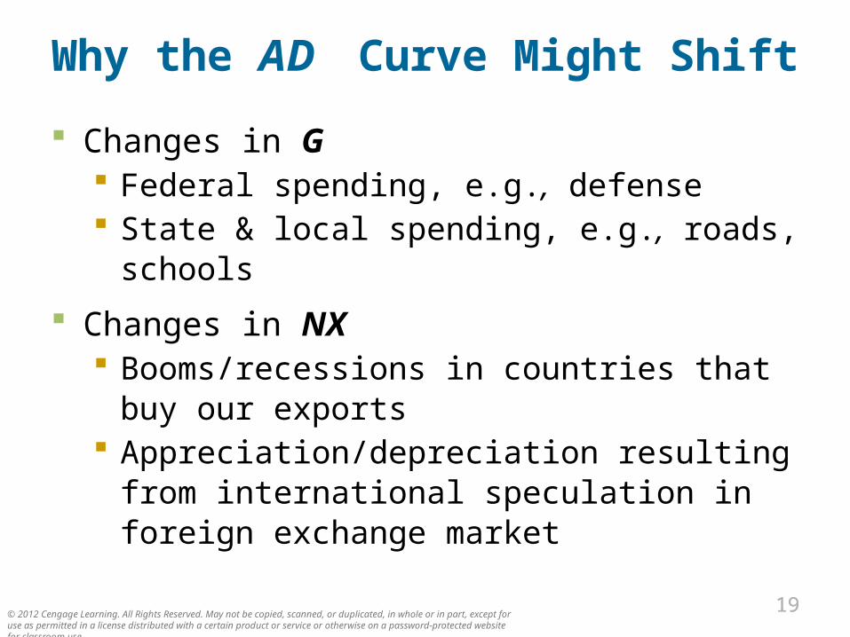
Why the AD Curve Might Shift
Changes in G Federal spending, e.g., defense State & local spending, e.g., roads, schools
Changes in NX Booms/recessions in countries that buy our
exports Appreciation/depreciation resulting from
international speculation in foreign exchange market
A C T I V E L E A R N I N G 1
The Aggregate-Demand curve
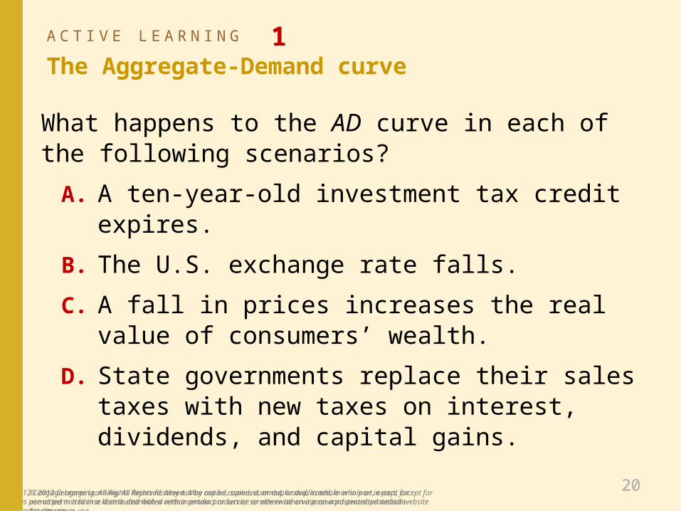
What happens to the AD curve in each of the following scenarios?
A. A ten-year-old investment tax credit expires.
B. The U.S. exchange rate falls.
C. A fall in prices increases the real value of consumers’ wealth.
D. State governments replace their sales taxes with new taxes on interest, dividends, and capital gains.
© 2012 Cengage Learning. All Rights Reserved. May not be copied, scanned, or duplicated, in whole or in part, except for use as permitted in a license distributed with a certain product or service or otherwise on a password-protected website for classroom use.
A C T I V E L E A R N I N G CLICKER QUESTION1
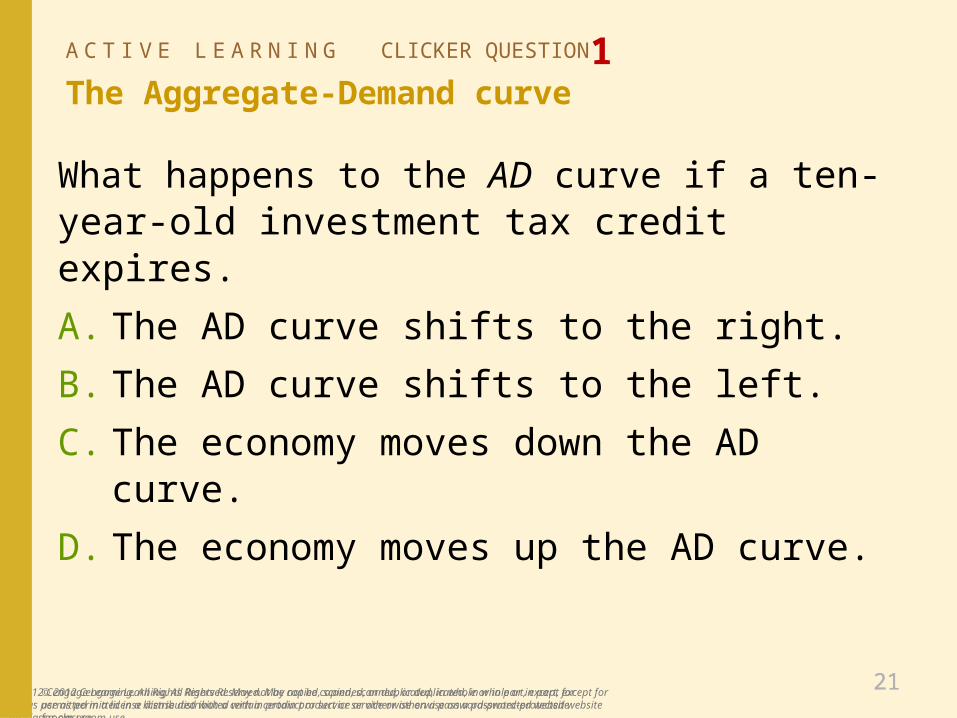
The Aggregate-Demand curve
What happens to the AD curve if a ten-year-old investment tax credit expires.
A. The AD curve shifts to the right.
B. The AD curve shifts to the left.
C. The economy moves down the AD curve.
D. The economy moves up the AD curve.
© 2012 Cengage Learning. All Rights Reserved. May not be copied, scanned, or duplicated, in whole or in part, except for use as permitted in a license distributed with a certain product or service or otherwise on a password-protected website for classroom use.
A C T I V E L E A R N I N G CLICKER QUESTION 2
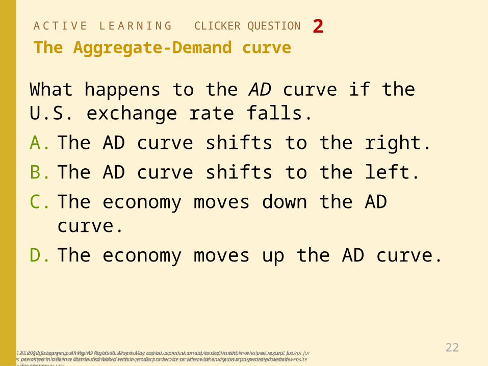
The Aggregate-Demand curve
What happens to the AD curve if the U.S. exchange rate falls.
A. The AD curve shifts to the right.
B. The AD curve shifts to the left.
C. The economy moves down the AD curve.
D. The economy moves up the AD curve.
© 2012 Cengage Learning. All Rights Reserved. May not be copied, scanned, or duplicated, in whole or in part, except for use as permitted in a license distributed with a certain product or service or otherwise on a password-protected website for classroom use.
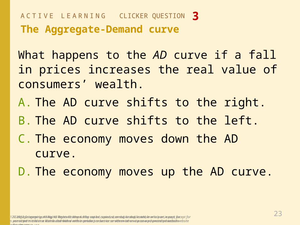
A C T I V E L E A R N I N G CLICKER QUESTION 3The Aggregate-Demand curve
What happens to the AD curve if a fall in prices increases the real value of consumers’ wealth.
A. The AD curve shifts to the right.
B. The AD curve shifts to the left.
C. The economy moves down the AD curve.
D. The economy moves up the AD curve.
© 2012 Cengage Learning. All Rights Reserved. May not be copied, scanned, or duplicated, in whole or in part, except for use as permitted in a license distributed with a certain product or service or otherwise on a password-protected website for classroom use.
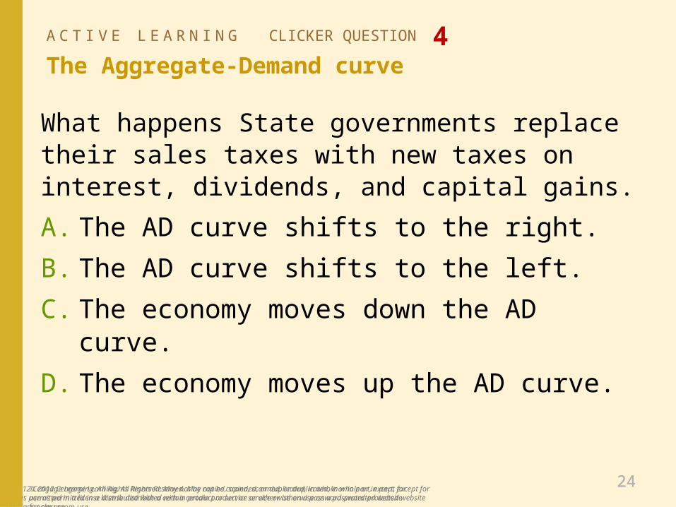
A C T I V E L E A R N I N G CLICKER QUESTION 4The Aggregate-Demand curve
What happens State governments replace their sales taxes with new taxes on interest, dividends, and capital gains.
A. The AD curve shifts to the right.
B. The AD curve shifts to the left.
C. The economy moves down the AD curve.
D. The economy moves up the AD curve.
© 2012 Cengage Learning. All Rights Reserved. May not be copied, scanned, or duplicated, in whole or in part, except for use as permitted in a license distributed with a certain product or service or otherwise on a password-protected website for classroom use.
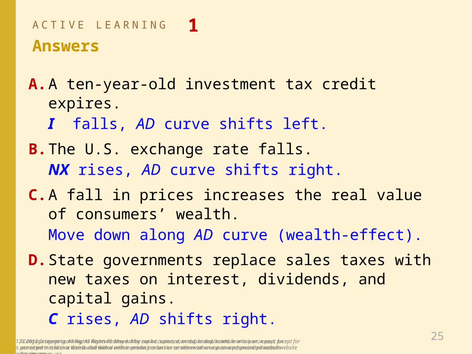
A C T I V E L E A R N I N G 1
Answers
A. A ten-year-old investment tax credit expires. I falls, AD curve shifts left.
B. The U.S. exchange rate falls. NX rises, AD curve shifts right.
C. A fall in prices increases the real value of consumers’ wealth. Move down along AD curve (wealth-effect).
D. State governments replace sales taxes with new taxes on interest, dividends, and capital gains. C rises, AD shifts right.
© 2012 Cengage Learning. All Rights Reserved. May not be copied, scanned, or duplicated, in whole or in part, except for use as permitted in a license distributed with a certain product or service or otherwise on a password-protected website for classroom use.
© 2012 Cengage Learning. All Rights Reserved. May not be copied, scanned, or duplicated, in whole or in part, except for use as permitted in a license distributed with a certain product or service or otherwise on a password-protected website for classroom use.
2626
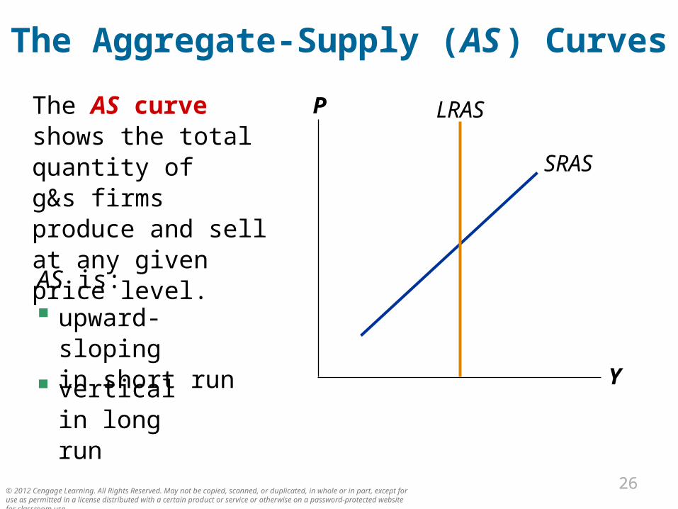
The Aggregate-Supply (AS ) Curves
The AS curve shows the total quantity of g&s firms produce and sell at any given price level.
P
Y
SRAS
LRAS
AS is:
upward-sloping in short run
vertical in long run
© 2012 Cengage Learning. All Rights Reserved. May not be copied, scanned, or duplicated, in whole or in part, except for use as permitted in a license distributed with a certain product or service or otherwise on a password-protected website for classroom use.
2727
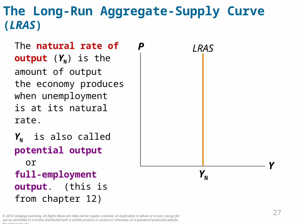
The Long-Run Aggregate-Supply Curve (LRAS)
The natural rate of output (YN) is the
amount of output the economy produces when unemployment is at its natural rate.
YN is also called
potential output or full-employment output. (this is from chapter 12)
P
Y
LRAS
YN
© 2012 Cengage Learning. All Rights Reserved. May not be copied, scanned, or duplicated, in whole or in part, except for use as permitted in a license distributed with a certain product or service or otherwise on a password-protected website for classroom use.
2828
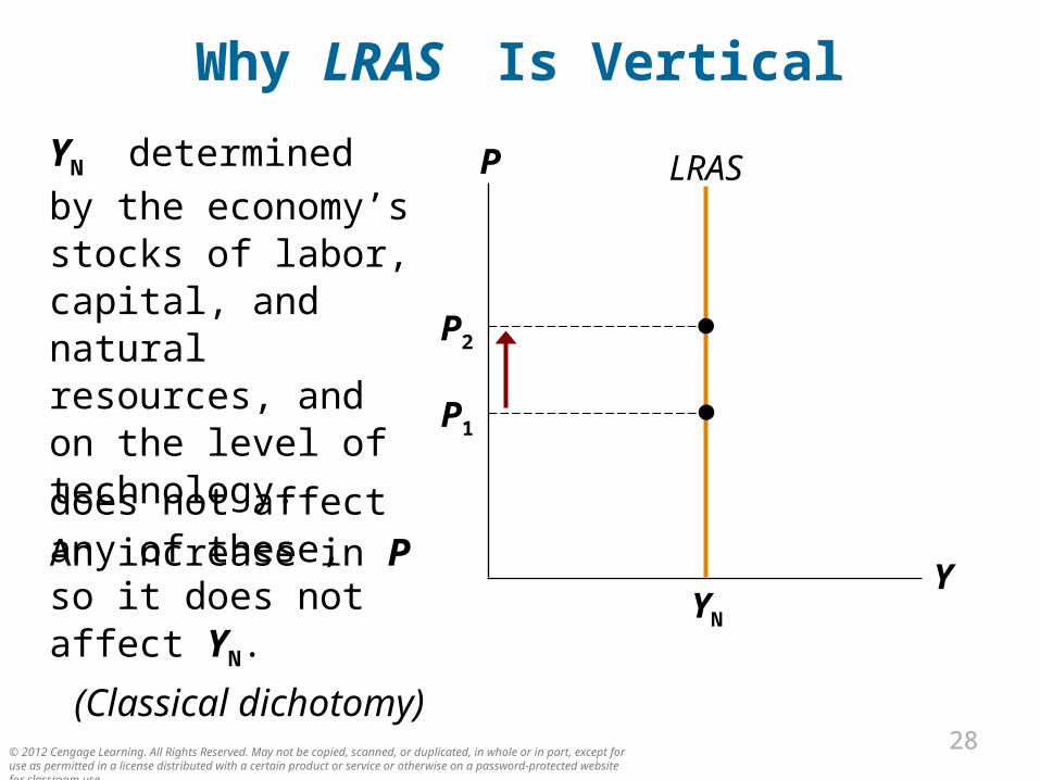
Why LRAS Is Vertical
YN determined by the
economy’s stocks of labor, capital, and natural resources, and on the level of technology.
An increase in P
P
Y
LRAS
P1
does not affect any of these, so it does not affect YN.
(Classical dichotomy)
P2
YN
© 2012 Cengage Learning. All Rights Reserved. May not be copied, scanned, or duplicated, in whole or in part, except for use as permitted in a license distributed with a certain product or service or otherwise on a password-protected website for classroom use.
2929
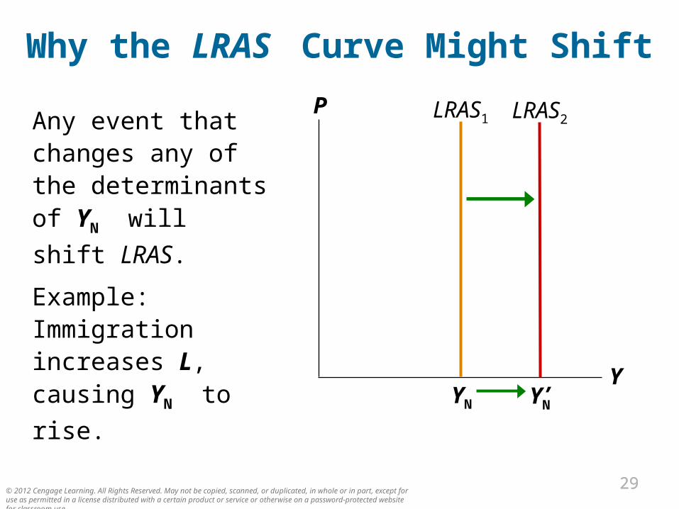
Why the LRAS Curve Might Shift
Any event that changes any of the determinants of YN
will shift LRAS.
Example: Immigration increases L, causing YN to rise.
P
Y
LRAS1
YN
LRAS2
YN’
© 2012 Cengage Learning. All Rights Reserved. May not be copied, scanned, or duplicated, in whole or in part, except for use as permitted in a license distributed with a certain product or service or otherwise on a password-protected website for classroom use.
3030
Why the LRAS Curve Might Shift
Changes in L or natural rate of unemployment Immigration Baby-boomers retire Govt policies reduce natural u-rate
Changes in K or H Investment in factories, equipment More people get college degrees Factories destroyed by a hurricane
© 2012 Cengage Learning. All Rights Reserved. May not be copied, scanned, or duplicated, in whole or in part, except for use as permitted in a license distributed with a certain product or service or otherwise on a password-protected website for classroom use.
3131
Why the LRAS Curve Might Shift
Changes in natural resources (N) Discovery of new mineral deposits Reduction in supply of imported oil Changing weather patterns that affect
agricultural production
Changes in technology (A) Productivity improvements from technological
progress
© 2012 Cengage Learning. All Rights Reserved. May not be copied, scanned, or duplicated, in whole or in part, except for use as permitted in a license distributed with a certain product or service or otherwise on a password-protected website for classroom use.
3232
LRAS1990
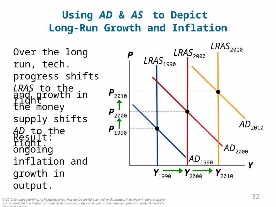
Using AD & AS to Depict Long-Run Growth and Inflation
Over the long run, tech. progress shifts LRAS to the right
P
Y
AD2000
LRAS2000
AD1990
Y2000
and growth in the money supply shifts AD to the right.
Y1990
AD2010
LRAS2010
Y2010
P1990Result: ongoing inflation and growth in output.
P2000
P2010
© 2012 Cengage Learning. All Rights Reserved. May not be copied, scanned, or duplicated, in whole or in part, except for use as permitted in a license distributed with a certain product or service or otherwise on a password-protected website for classroom use.
3333
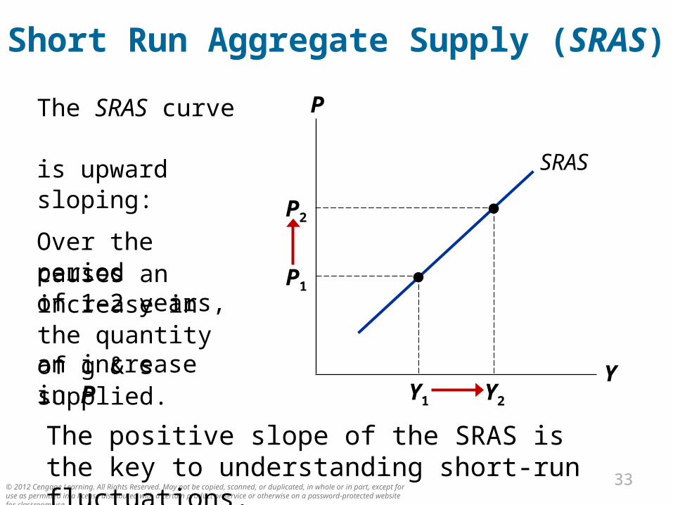
Short Run Aggregate Supply (SRAS)
The SRAS curve is upward sloping:
Over the period of 1–2 years, an increase in P
P
Y
SRAS
causes an increase in the quantity of g & s supplied.
Y2
P1
Y1
P2
The positive slope of the SRAS is the key to understanding short-run fluctuations.
© 2012 Cengage Learning. All Rights Reserved. May not be copied, scanned, or duplicated, in whole or in part, except for use as permitted in a license distributed with a certain product or service or otherwise on a password-protected website for classroom use.
3434
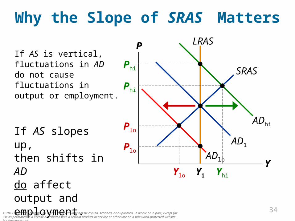
Why the Slope of SRAS Matters
If AS is vertical, fluctuations in AD do not cause fluctuations in output or employment.
P
Y
AD1
SRAS
LRAS
ADhi
ADlo
Y1
If AS slopes up, then shifts in AD do affect output and employment.
Plo
Ylo
Phi
Yhi
Phi
Plo
© 2012 Cengage Learning. All Rights Reserved. May not be copied, scanned, or duplicated, in whole or in part, except for use as permitted in a license distributed with a certain product or service or otherwise on a password-protected website for classroom use.
3535
Three Theories of SRASIn each,
some type of market imperfection (maybe better, some type of confusion)
result: Output deviates from its natural rate when the actual price level deviates from the price level people expected.
© 2012 Cengage Learning. All Rights Reserved. May not be copied, scanned, or duplicated, in whole or in part, except for use as permitted in a license distributed with a certain product or service or otherwise on a password-protected website for classroom use.
3636
1. The Sticky-Wage Theory
Imperfection: Nominal wages are sticky in the short run,they adjust sluggishly. Due to labor contracts, social norms
Firms and workers set the nominal wage in advance based on PE, the price level they
expect to prevail.
© 2012 Cengage Learning. All Rights Reserved. May not be copied, scanned, or duplicated, in whole or in part, except for use as permitted in a license distributed with a certain product or service or otherwise on a password-protected website for classroom use.
3737
1. The Sticky-Wage Theory
If P > PE,
revenue is higher, but labor cost is not.
Production is more profitable, so firms increase output and employment.
Hence, higher P causes higher Y, so the SRAS curve slopes upward.
© 2012 Cengage Learning. All Rights Reserved. May not be copied, scanned, or duplicated, in whole or in part, except for use as permitted in a license distributed with a certain product or service or otherwise on a password-protected website for classroom use.
3838
2. The Sticky-Price Theory
Imperfection: Many prices are sticky in the short run. Due to menu costs, the costs of adjusting
prices. Examples: cost of printing new menus,
the time required to change price tags
Firms set sticky prices in advance based on PE.
© 2012 Cengage Learning. All Rights Reserved. May not be copied, scanned, or duplicated, in whole or in part, except for use as permitted in a license distributed with a certain product or service or otherwise on a password-protected website for classroom use.
3939
2. The Sticky-Price Theory
Suppose the Fed increases the money supply unexpectedly. In the long run, P will rise.
In the short run, firms without menu costs can raise their prices immediately.
Firms with menu costs wait to raise prices. Meanwhile, their prices are relatively low, which increases demand for their products,so they increase output and employment.
Hence, higher P is associated with higher Y, so the SRAS curve slopes upward.
© 2012 Cengage Learning. All Rights Reserved. May not be copied, scanned, or duplicated, in whole or in part, except for use as permitted in a license distributed with a certain product or service or otherwise on a password-protected website for classroom use.
4040
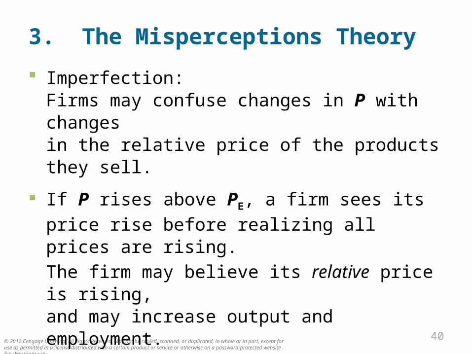
3. The Misperceptions Theory
Imperfection: Firms may confuse changes in P with changes in the relative price of the products they sell.
If P rises above PE, a firm sees its price rise before
realizing all prices are rising.
The firm may believe its relative price is rising, and may increase output and employment.
So, an increase in P can cause an increase in Y, making the SRAS curve upward-sloping.
© 2012 Cengage Learning. All Rights Reserved. May not be copied, scanned, or duplicated, in whole or in part, except for use as permitted in a license distributed with a certain product or service or otherwise on a password-protected website for classroom use.
4141
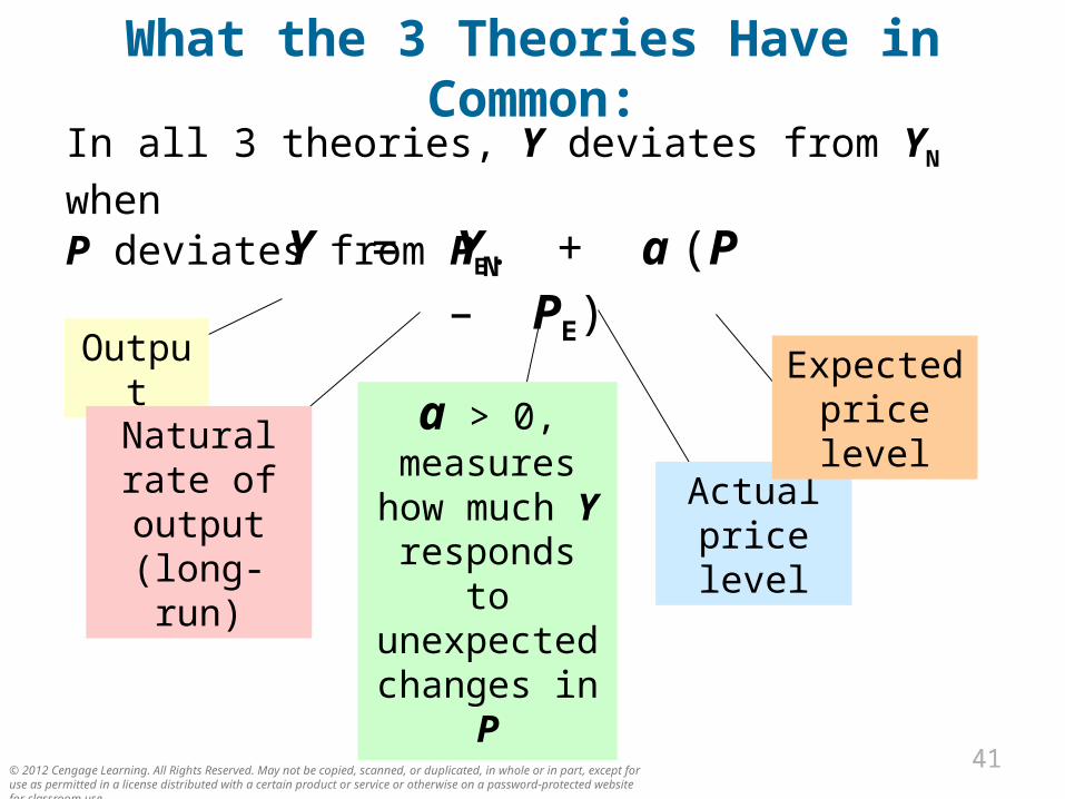
What the 3 Theories Have in Common:
In all 3 theories, Y deviates from YN when
P deviates from PE.
Y = YN + a (P – PE)Output
Natural rate of output (long-run)
a > 0, measures
how much Y responds to unexpected
changes in P
Actual price level
Expected price level
© 2012 Cengage Learning. All Rights Reserved. May not be copied, scanned, or duplicated, in whole or in part, except for use as permitted in a license distributed with a certain product or service or otherwise on a password-protected website for classroom use.
4242
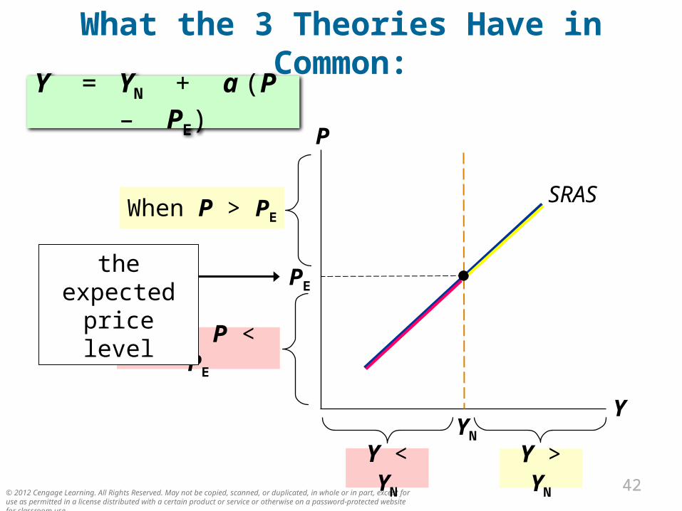
What the 3 Theories Have in Common:
P
Y
SRAS
YN
When P > PE
Y > YN
When P < PE
Y < YN
PE
the expected price level
Y = YN + a (P – PE)
© 2012 Cengage Learning. All Rights Reserved. May not be copied, scanned, or duplicated, in whole or in part, except for use as permitted in a license distributed with a certain product or service or otherwise on a password-protected website for classroom use.
4343
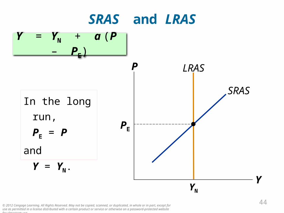
SRAS and LRAS
The imperfections in these theories are temporary. Over time, sticky wages and prices become flexible misperceptions are corrected
In the LR, PE = P AS curve is vertical
© 2012 Cengage Learning. All Rights Reserved. May not be copied, scanned, or duplicated, in whole or in part, except for use as permitted in a license distributed with a certain product or service or otherwise on a password-protected website for classroom use.
4444
LRAS
SRAS and LRAS
P
Y
SRAS
PE
YN
In the long run,
PE = P
and
Y = YN.
Y = YN + a (P – PE)
© 2012 Cengage Learning. All Rights Reserved. May not be copied, scanned, or duplicated, in whole or in part, except for use as permitted in a license distributed with a certain product or service or otherwise on a password-protected website for classroom use.
4545
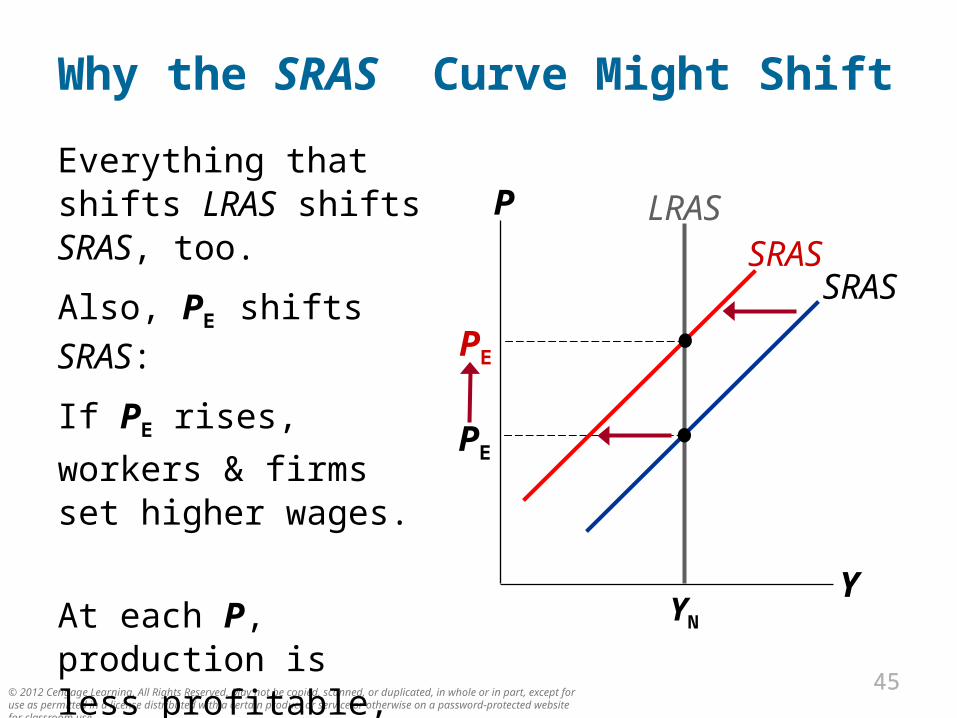
Why the SRAS Curve Might Shift
Everything that shifts LRAS shifts SRAS, too.
Also, PE shifts SRAS:
If PE rises,
workers & firms set higher wages.
At each P, production is less profitable, Y falls, SRAS shifts left.
LRASP
Y
SRAS
PE
YN
SRAS
PE
© 2012 Cengage Learning. All Rights Reserved. May not be copied, scanned, or duplicated, in whole or in part, except for use as permitted in a license distributed with a certain product or service or otherwise on a password-protected website for classroom use.
4646
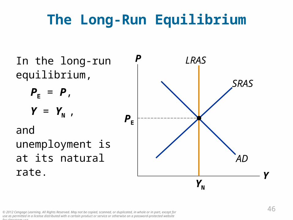
The Long-Run Equilibrium
In the long-run equilibrium,
PE = P,
Y = YN ,
and unemployment is at its natural rate.
P
Y
AD
SRAS
PE
LRAS
YN
© 2012 Cengage Learning. All Rights Reserved. May not be copied, scanned, or duplicated, in whole or in part, except for use as permitted in a license distributed with a certain product or service or otherwise on a password-protected website for classroom use.
4747
Economic Fluctuations
Caused by events that shift the AD and/or AS curves.
Four steps to analyzing economic fluctuations:
1. Determine whether the event shifts AD or AS.
2. Determine whether curve shifts left or right.
3. Use AD–AS diagram to see how the shift changes Y and P in the short run.
4. Use AD–AS diagram to see how economy moves from new SR eq’m to new LR eq’m.
© 2012 Cengage Learning. All Rights Reserved. May not be copied, scanned, or duplicated, in whole or in part, except for use as permitted in a license distributed with a certain product or service or otherwise on a password-protected website for classroom use.
4848
LRAS
YN
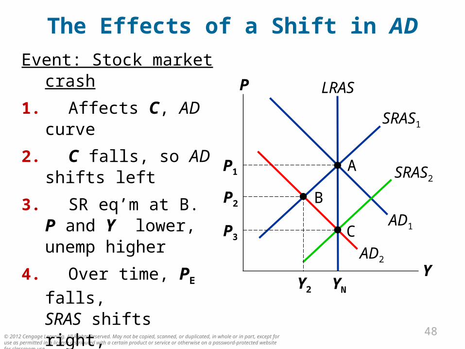
The Effects of a Shift in AD
Event: Stock market crash
1. Affects C, AD curve
2. C falls, so AD shifts left
3. SR eq’m at B. P and Y lower,unemp higher
4. Over time, PE falls,
SRAS shifts right,until LR eq’m at C.Y and unemp back at initial levels.
P
Y
AD1
SRAS1
AD2
SRAS2P1 A
P2
Y2
B
P3 C
© 2012 Cengage Learning. All Rights Reserved. May not be copied, scanned, or duplicated, in whole or in part, except for use as permitted in a license distributed with a certain product or service or otherwise on a password-protected website for classroom use.
4949
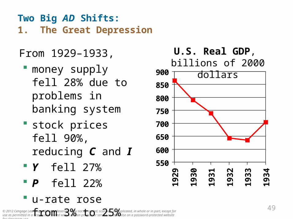
Two Big AD Shifts: 1. The Great Depression
From 1929–1933, money supply fell
28% due to problems in banking system
stock prices fell 90%, reducing C and I
Y fell 27% P fell 22% u-rate rose
from 3% to 25%
550
600
650
700
750
800
850
900
19
29
19
30
19
31
19
32
19
33
19
34
U.S. Real GDP, billions of 2000 dollars
© 2012 Cengage Learning. All Rights Reserved. May not be copied, scanned, or duplicated, in whole or in part, except for use as permitted in a license distributed with a certain product or service or otherwise on a password-protected website for classroom use.
5050
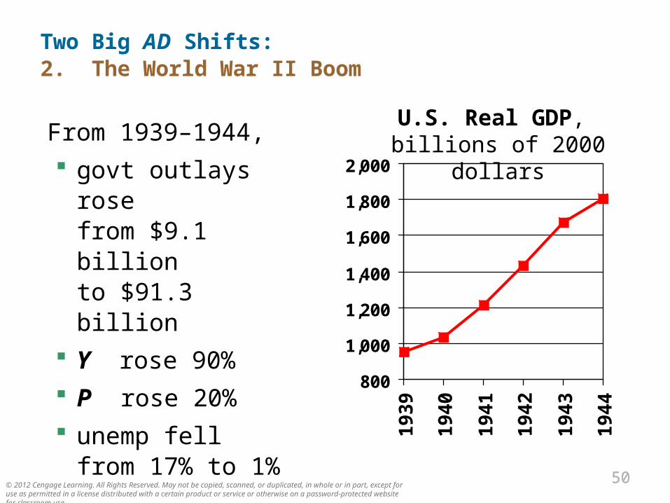
Two Big AD Shifts: 2. The World War II Boom
From 1939–1944,
govt outlays rose from $9.1 billion to $91.3 billion
Y rose 90%
P rose 20%
unemp fell from 17% to 1% 800
1,000
1,200
1,400
1,600
1,800
2,000
19
39
19
40
19
41
19
42
19
43
19
44
U.S. Real GDP, billions of 2000 dollars
A C T I V E L E A R N I N G 2
Working with the model
Draw the AD-SRAS-LRAS diagram for the U.S. economy starting in a long-run equilibrium.
A boom occurs in Canada. Use your diagram to determine the SR and LR effects on U.S. GDP, the price level, and unemployment.
© 2012 Cengage Learning. All Rights Reserved. May not be copied, scanned, or duplicated, in whole or in part, except for use as permitted in a license distributed with a certain product or service or otherwise on a password-protected website for classroom use.
A C T I V E L E A R N I N G 2
Answers
© 2012 Cengage Learning. All Rights Reserved. May not be copied, scanned, or duplicated, in whole or in part, except for use as permitted in a license distributed with a certain product or service or otherwise on a password-protected website for classroom use.
LRAS
YN
P
Y
AD2
SRAS2
AD1
SRAS1
P1
P3 C
P2
Y2
B
A
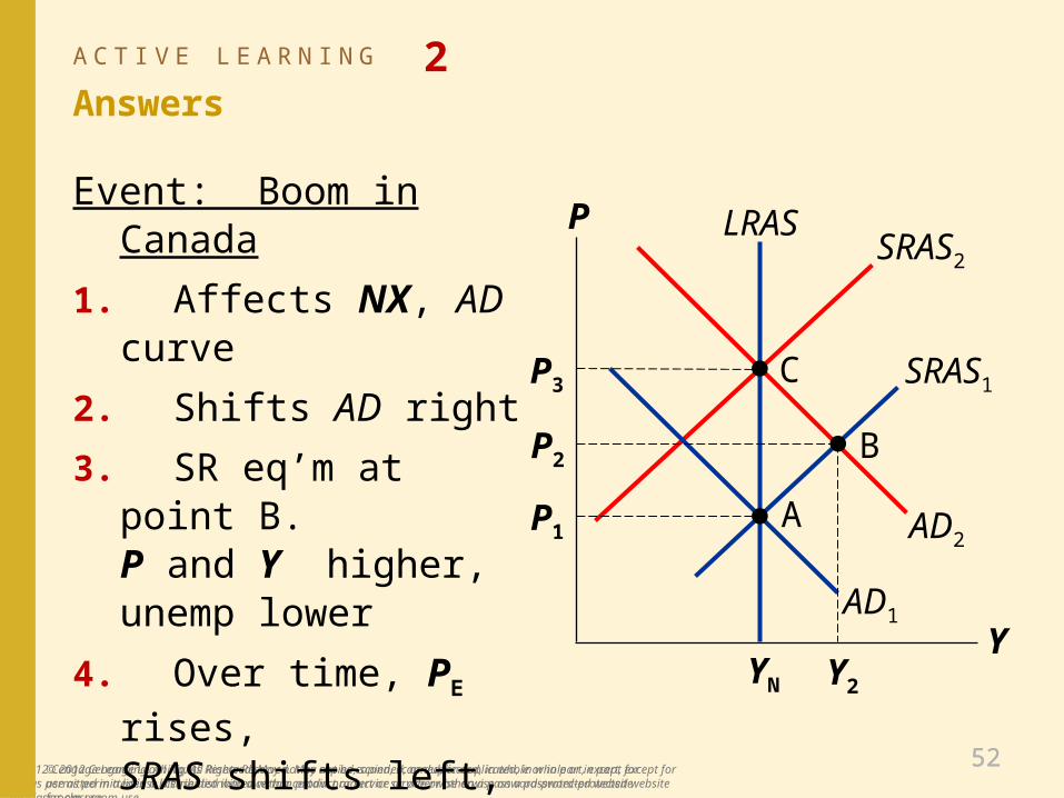
Event: Boom in Canada
1. Affects NX, AD curve
2. Shifts AD right
3. SR eq’m at point B. P and Y higher,unemp lower
4. Over time, PE rises,
SRAS shifts left,until LR eq’m at C.Y and unemp back at initial levels.
© 2012 Cengage Learning. All Rights Reserved. May not be copied, scanned, or duplicated, in whole or in part, except for use as permitted in a license distributed with a certain product or service or otherwise on a password-protected website for classroom use.
5353
CASE STUDY: The 2008–2009 Recession From 12/2007 to 6/2009, real GDP fell about 4%
Unemployment rose from 4.4% in 5/2007 to 10.1% in 10/2009
The housing market played a central role in this recession…
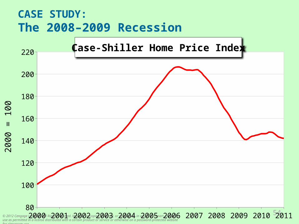
CASE STUDY: The 2008–2009 Recession
2000 2001 2002 2003 2004 2005 2006 2007 2008 2009 2010 201180
100
120
140
160
180
200
220 Case-Shiller Home Price Index
2000
= 1
00
© 2012 Cengage Learning. All Rights Reserved. May not be copied, scanned, or duplicated, in whole or in part, except for use as permitted in a license distributed with a certain product or service or otherwise on a password-protected website for classroom use.
5555
CASE STUDY: The 2008–2009 Recession
Rising house prices during 2002–2006 due to:
low interest rates
easier credit for “sub-prime” borrowers
government policies to increase homeownership
securitization of mortgages: Investment banks purchased mortgages from
lenders, created securities backed by these mortgages, sold the securities to banks, insurance companies, and other investors.
Mortgage-backed securities perceived as safe, since house prices “never fall”
© 2012 Cengage Learning. All Rights Reserved. May not be copied, scanned, or duplicated, in whole or in part, except for use as permitted in a license distributed with a certain product or service or otherwise on a password-protected website for classroom use.
5656
CASE STUDY: CLICKER QUESTION!!The 2008–2009 Recession
In the short run, rising house prices during 2002–2006 would
A. Shift the AD curve out because of the effects on C.
B. Shift the AD curve out because of the effects on I.
C. Shift the AD curve out because of the effects on NX.
D. Shift the SRAS curve out because of the effects on price expectations.
© 2012 Cengage Learning. All Rights Reserved. May not be copied, scanned, or duplicated, in whole or in part, except for use as permitted in a license distributed with a certain product or service or otherwise on a password-protected website for classroom use.
5757
CASE STUDY: The 2008–2009 Recession
Consequences of 2006–2009 housing market crash:
Millions of homeowners “underwater”—owed more than house was worth
Millions of mortgage defaults and foreclosures
Banks selling foreclosed houses increased surplus and downward price pressures
Housing crash badly damaged construction industry: 2010 unemployment rate was 20.6% in construction vs. 9.6% overall
© 2012 Cengage Learning. All Rights Reserved. May not be copied, scanned, or duplicated, in whole or in part, except for use as permitted in a license distributed with a certain product or service or otherwise on a password-protected website for classroom use.
5858
CASE STUDY: CLICKER QUESTION!!The 2008–2009 Recession
In the short run, the 2006–2009 housing crash would
A. Shift the AD curve in because of the effects on C.
B. Shift the AD curve in because of the effects on I.
C. Shift the AD curve in because of the effects on NX.
D. Shift the SRAS curve in because of the effects on price expectations.
© 2012 Cengage Learning. All Rights Reserved. May not be copied, scanned, or duplicated, in whole or in part, except for use as permitted in a license distributed with a certain product or service or otherwise on a password-protected website for classroom use.
5959
CASE STUDY: The 2008–2009 Recession
Consequences of 2006–2009 housing market crash:
Mortgage-backed securities became “toxic,” heavy losses for institutions that purchased them, widespread failures of banks and other financial institutions
Sharply rising unemployment and falling GDP
© 2012 Cengage Learning. All Rights Reserved. May not be copied, scanned, or duplicated, in whole or in part, except for use as permitted in a license distributed with a certain product or service or otherwise on a password-protected website for classroom use.
6060
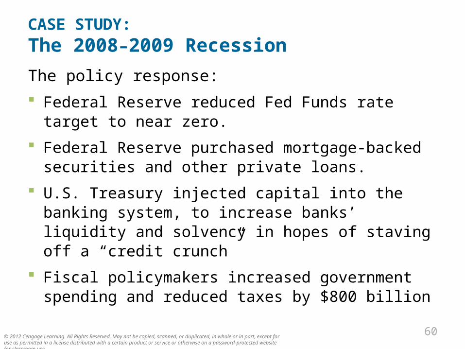
CASE STUDY: The 2008–2009 Recession
The policy response:
Federal Reserve reduced Fed Funds rate target to near zero.
Federal Reserve purchased mortgage-backed securities and other private loans.
U.S. Treasury injected capital into the banking system, to increase banks’ liquidity and solvency in hopes of staving off a “credit crunch”
Fiscal policymakers increased government spending and reduced taxes by $800 billion
© 2012 Cengage Learning. All Rights Reserved. May not be copied, scanned, or duplicated, in whole or in part, except for use as permitted in a license distributed with a certain product or service or otherwise on a password-protected website for classroom use.
6161
CASE STUDY: CLICKER QUESTION!!!The 2008–2009 Recession
The three policy responses -- Federal Reserve reduced Fed Funds rate target, purchased private loans and the U.S. Treasury increased banks’ liquidity, were mainly intended to
A. Maintain or increase C.
B. Maintain or increase I.
C. Maintain or increase NX.
D. Maintain or increase G.
© 2012 Cengage Learning. All Rights Reserved. May not be copied, scanned, or duplicated, in whole or in part, except for use as permitted in a license distributed with a certain product or service or otherwise on a password-protected website for classroom use.
6262
CASE STUDY: CLICKER QUESTION!!!The 2008–2009 Recession
The effect of the three policy responses was to
A. Shift the SRAS curve in.
B. Shift the SRAS curve out.
C. Shift the AD curve in.
D. Shift the AD curve out.
© 2012 Cengage Learning. All Rights Reserved. May not be copied, scanned, or duplicated, in whole or in part, except for use as permitted in a license distributed with a certain product or service or otherwise on a password-protected website for classroom use.
6363
CASE STUDY: CLICKER QUESTION!!!The 2008–2009 Recession
The effect of the increase in government spending was to
A. Shift the SRAS curve in.
B. Shift the SRAS curve out.
C. Shift the AD curve in.
D. Shift the AD curve out.
© 2012 Cengage Learning. All Rights Reserved. May not be copied, scanned, or duplicated, in whole or in part, except for use as permitted in a license distributed with a certain product or service or otherwise on a password-protected website for classroom use.
6464
LRAS
YN
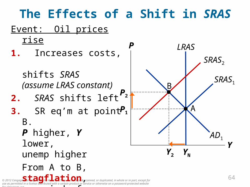
The Effects of a Shift in SRASEvent: Oil prices rise
1. Increases costs, shifts SRAS(assume LRAS constant)
2. SRAS shifts left
3. SR eq’m at point B. P higher, Y lower,unemp higher
From A to B, stagflation, a period of falling output and rising prices.
P
YAD1
SRAS1
SRAS2
P1A
P2
Y2
B
© 2012 Cengage Learning. All Rights Reserved. May not be copied, scanned, or duplicated, in whole or in part, except for use as permitted in a license distributed with a certain product or service or otherwise on a password-protected website for classroom use.
6565
LRAS
YN
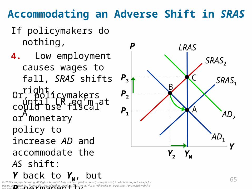
Accommodating an Adverse Shift in SRAS
If policymakers do nothing,
4. Low employment causes wages to fall, SRAS shifts right,until LR eq’m at A.
P
YAD1
SRAS1
SRAS2
P1A
P2
Y2
B
AD2
P3 C
Or, policymakers could use fiscal or monetary policy to increase AD and accommodate the AS shift: Y back to YN, but
P permanently higher.
© 2012 Cengage Learning. All Rights Reserved. May not be copied, scanned, or duplicated, in whole or in part, except for use as permitted in a license distributed with a certain product or service or otherwise on a password-protected website for classroom use.
6666
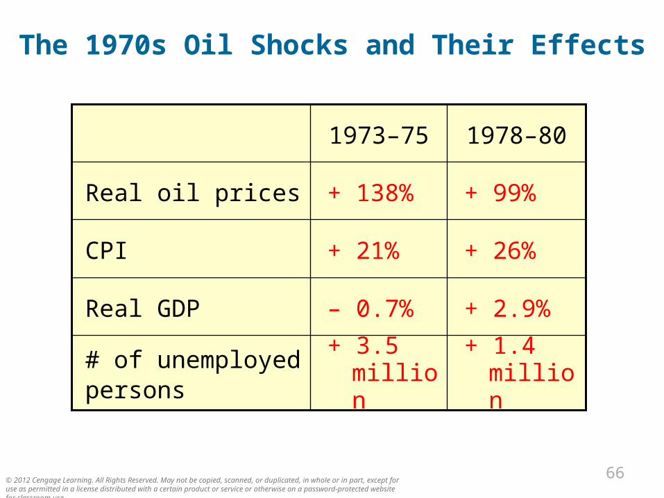
The 1970s Oil Shocks and Their Effects
# of unemployed persons
Real GDP
CPI
+ 1.4 million
+ 2.9%
+ 26%
+ 99%
+ 3.5 million
– 0.7%
+ 21%
+ 138%Real oil prices
1978–801973–75

© 2012 Cengage Learning. All Rights Reserved. May not be copied, scanned, or duplicated, in whole or in part, except for use as permitted in a license distributed with a certain product or service or otherwise on a password-protected website for classroom use.
6767
John Maynard Keynes, 1883–1946
The General Theory of Employment, Interest, and Money, 1936
Argued recessions and depressions can result from inadequate demand; policymakers should shift AD.
Famous critique of classical theory:
Economists set themselves too easy, too useless a task if in tempestuous seasons they can only tell us when the storm is long past, the ocean will be flat.
The long run is a misleading guide to current affairs. In the long run, we are all dead.
© 2012 Cengage Learning. All Rights Reserved. May not be copied, scanned, or duplicated, in whole or in part, except for use as permitted in a license distributed with a certain product or service or otherwise on a password-protected website for classroom use.
6868
CONCLUSION
This chapter has introduced the model of aggregate demand and aggregate supply, which helps explain economic fluctuations.
Keep in mind: these fluctuations are deviations from the long-run trends explained by the models we learned in previous chapters.
In the next chapter, we will learn how policymakers can affect aggregate demand with fiscal and monetary policy.
S U M M A RY
• Short-run fluctuations in GDP and other macroeconomic quantities are irregular and unpredictable. Recessions are periods of falling real GDP and rising unemployment.
• Economists analyze fluctuations using the model of aggregate demand and aggregate supply.
• The aggregate demand curve slopes downward because a change in the price level has a wealth effect on consumption, an interest-rate effect on investment, and an exchange-rate effect on net exports.
© 2012 Cengage Learning. All Rights Reserved. May not be copied, scanned, or duplicated, in whole or in part, except for use as permitted in a license distributed with a certain product or service or otherwise on a password-protected website for classroom use.
S U M M A RY
• Anything that changes C, I, G, or NX—except a change in the price level—will shift the aggregate demand curve.
• The long-run aggregate supply curve is vertical because changes in the price level do not affect output in the long run.
• In the long run, output is determined by labor, capital, natural resources, and technology; changes in any of these will shift the long-run aggregate supply curve.
© 2012 Cengage Learning. All Rights Reserved. May not be copied, scanned, or duplicated, in whole or in part, except for use as permitted in a license distributed with a certain product or service or otherwise on a password-protected website for classroom use.
S U M M A RY
• In the short run, output deviates from its natural rate when the price level is different than expected, leading to an upward-sloping short-run aggregate supply curve. The three theories proposed to explain this upward slope are the sticky wage theory, the sticky price theory, and the misperceptions theory.
• The short-run aggregate-supply curve shifts in response to changes in the expected price level and to anything that shifts the long-run aggregate supply curve.
© 2012 Cengage Learning. All Rights Reserved. May not be copied, scanned, or duplicated, in whole or in part, except for use as permitted in a license distributed with a certain product or service or otherwise on a password-protected website for classroom use.
S U M M A RY
• Economic fluctuations are caused by shifts in aggregate demand and aggregate supply.
• When aggregate demand falls, output and the price level fall in the short run. Over time, a change in expectations causes wages, prices, and perceptions to adjust, and the short-run aggregate supply curve shifts rightward. In the long run, the economy returns to the natural rates of output and unemployment, but with a lower price level.
© 2012 Cengage Learning. All Rights Reserved. May not be copied, scanned, or duplicated, in whole or in part, except for use as permitted in a license distributed with a certain product or service or otherwise on a password-protected website for classroom use.
S U M M A RY
• A fall in aggregate supply results in stagflation—falling output and rising prices. Wages, prices, and perceptions adjust over time, and the economy recovers.
© 2012 Cengage Learning. All Rights Reserved. May not be copied, scanned, or duplicated, in whole or in part, except for use as permitted in a license distributed with a certain product or service or otherwise on a password-protected website for classroom use.