Eva Hromadkova PowerPoint ® Slides by Ron Cronovich CHAPTER ELEVEN Aggregate Demand II macro © 2002 Worth Publishers, all rights reserved Topic 12a: Aggregate

Eva Hromadkova

PowerPoint® Slides by Ron Cronovich

CHAPTER ELEVEN

Aggregate Demand IIm

acro

© 2002 Worth Publishers, all rights reserved

Topic 12a:

Aggregate Demand II(chapter 11, Mankiw)

CHAPTER 11CHAPTER 11 Aggregate Demand II Aggregate Demand II slide 2

ContextContext

Chapter 9 introduced the model of aggregate demand and supply.

Chapter 10 developed the IS-LM model, the basis of the aggregate demand curve.

In Chapter 11, we will use the IS-LM model to– see how policies and shocks affect

income and the interest rate in the short run when prices are fixed

– derive the aggregate demand curve– explore various explanations for the

Great Depression


The intersection determines the unique combination of Y and r that satisfies equilibrium in both markets.

The LM curve represents money market equilibrium.

Equilibrium in the Equilibrium in the ISIS--LMLM ModelModel

The IS curve represents equilibrium in the goods market.

( ) ( )Y C Y T I r G

( , )M P L r Y ISY

rLM

r1

Y1


causing output & income to rise.

IS1

An increase in government purchasesAn increase in government purchases

1. IS curve shifts right

Y

rLM

r1

Y1

1by

1 MPCG

IS2

Y2

r2

1.2. This raises money

demand, causing the interest rate to rise…

2.

3. …which reduces investment, so the final increase in Y 1is smaller than

1 MPCG

3.


IS1

1.

A tax cutA tax cut

Y

rLM

r1

Y1

IS2

Y2

r2

Because consumers save (1MPC) of the tax cut, the initial boost in spending is smaller for T than for an equal G…

and the IS curve shifts by

MPC1 MPC

T

1.

2.

2.…so the effects on r and Y are smaller for a T than for an equal G.

2.


2. …causing the interest rate to fall

IS

Monetary Policy: an increase in Monetary Policy: an increase in MM

1. M > 0 shifts the LM curve down(or to the right)

Y

r LM1

r1

Y1 Y2

r2

LM2

3. …which increases investment, causing output & income to rise.


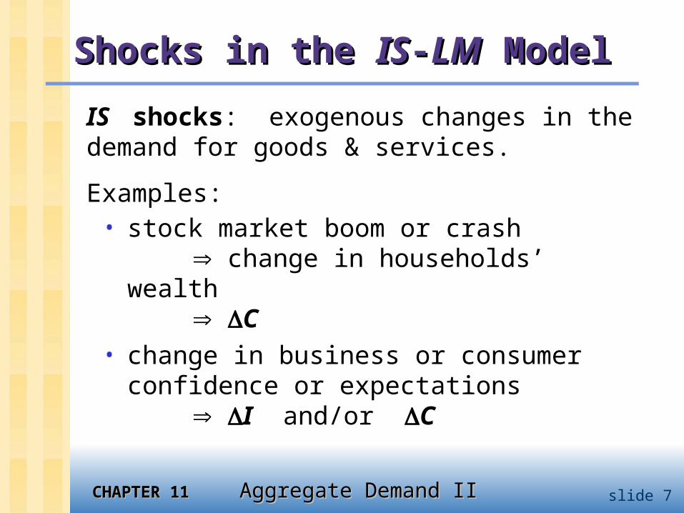
Shocks in the Shocks in the ISIS--LMLM Model Model

IS shocks: exogenous changes in the demand for goods & services.

Examples: • stock market boom or crash

change in households’ wealth C

• change in business or consumer confidence or expectations I and/or C


Shocks in the Shocks in the ISIS--LMLM Model Model

LM shocks: exogenous changes in the demand for money.

Examples:• a wave of credit card fraud increases

demand for money• more ATMs or the Internet banking

reduce money demand


CASE STUDYCASE STUDY The U.S. economic slowdown of 2001The U.S. economic slowdown of 2001

~What happened~

1. Real GDP growth rate1994-2000: 3.9% (average

annual)2001: 1.2%

2. Unemployment rateDec 2000: 4.0%

Dec 2001: 5.8%



~Shocks that contributed to the slowdown~

1. Falling stock prices (dotcom bubble) From Aug 2000 to Aug 2001: -25%

Week after 9/11: -12%

2. The terrorist attacks on 9/11• increased uncertainty • fall in consumer & business confidence

Both shocks reduced spending and shifted the IS curve left.



~The policy response~1. Fiscal policy

• large long-term tax cut, immediate $300 tax rebate checks

• spending increases:aid to New York City & the airline industry,war on terrorism

2. Monetary policy• Fed lowered its Fed Funds rate target

11 times during 2001, from 6.5% to 1.75%• Money growth increased, interest rates

fell


What is the Fed’s policy instrument?What is the Fed’s policy instrument?

What the newspaper says:“the Fed lowered interest rates by one-half point today”

What actually happened:The Fed conducted expansionary monetary policy to shift the LM curve to the right until the interest rate fell 0.5 points.

The Fed The Fed targetstargets the Federal Funds rate: the Federal Funds rate: it announces a target value, it announces a target value,

and uses monetary policy to shift the LM and uses monetary policy to shift the LM curve curve

as needed to attain its target rate. as needed to attain its target rate.

The Fed The Fed targetstargets the Federal Funds rate: the Federal Funds rate: it announces a target value, it announces a target value,

and uses monetary policy to shift the LM and uses monetary policy to shift the LM curve curve

as needed to attain its target rate. as needed to attain its target rate.


IS-LM and Aggregate DemandIS-LM and Aggregate Demand

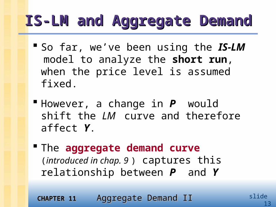
So far, we’ve been using the IS-LM

model to analyze the short run, when the price level is assumed fixed.

However, a change in P would shift the LM curve and therefore affect Y.

The aggregate demand curve (introduced in chap. 9 ) captures this relationship between P and Y


Y1Y2

Deriving the Deriving the ADAD curve curve

Y

r

Y

P

IS

LM(P1)

LM(P2)

AD

P1

P2

Y2 Y1

r2

r1

Intuition for slope of AD curve:

P (M/P )

LM shifts left

r

I

Y


Monetary policy and the Monetary policy and the ADAD curve curve

Y

P

IS

LM(M2/P1)

LM(M1/P1)

AD1

P1

Y1

Y1

Y2

Y2

r1

r2

The Fed can increase aggregate demand:

M LM shifts right

AD2

Y

r

r

I

Y at each value of P


Y2

Y2

r2

Y1

Y1

r1

Fiscal policy and the Fiscal policy and the ADAD curve curve

Y

r

Y

P

IS1

LM

AD1

P1

Expansionary fiscal policy (G and/or T ) increases agg. demand:

T C

IS shifts right

Y at each value of P AD2

IS2


Policy EffectivenessPolicy EffectivenessFiscal policy is effective (Y will rise much) when:

LM flatterAs the rise in G raises Y,

the increase in money demand does not raise r much:

so investment is not crowded out as much.

LM’

Y2’

2’

Y2

IS2

2

LM

Y1

IS1r

1


Policy EffectivenessPolicy EffectivenessMonetary policy is effective (Y will rise much) when:

IS flatter

As a rise in M lowers the interest rate (r),

investment rises more in response to the fall in r,

so output rises more.Y2

LM2

2

Y1

LM1

r

1

Y2’

2’

IS

IS’


IS-LMIS-LM and and AD-AS AD-AS in the short run & long runin the short run & long run

Recall from Chapter 9: The force that moves the economy from the short run to the long run is the gradual adjustment of prices.

Y Y

Y Y

Y Y

rise

fall

remain constant

In the short-run equilibrium, if

then over time, the price level

will


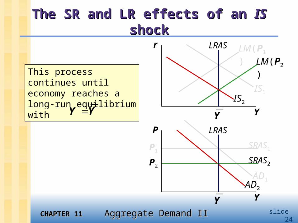
The SR and LR effects of an The SR and LR effects of an ISIS shock shock

A negative IS shock shifts IS and AD left, causing Y to fall. Y

r

Y

P LRAS

Y

LRAS

Y

IS1

SRAS1P1

LM(P1)

IS2

AD2

AD1



Y

r

Y

P LRAS

Y

LRAS

Y

IS1

SRAS1P1

LM(P1)

IS2

AD2

AD1

In the new short-run equilibrium, Y Y



Y

r

Y

P LRAS

Y

LRAS

Y

IS1

SRAS1P1

LM(P1)

IS2

AD2

AD1

In the new short-run equilibrium, Y Y

Over time, P gradually falls, which causes• SRAS to move

down• M/P to increase,

which causes LM to move down


AD2


Y

r

Y

P LRAS

Y

LRAS

Y

IS1

SRAS1P1

LM(P1)

IS2

AD1

Over time, P gradually falls, which causes• SRAS to move

down• M/P to increase,

which causes LM to move down

SRAS2P2

LM(P2)


AD2

SRAS2P2

LM(P2)


Y

r

Y

P LRAS

Y

LRAS

Y

IS1

SRAS1P1

LM(P1)

IS2

AD1

This process continues until economy reaches a long-run equilibrium with Y Y


The Great DepressionThe Great Depression

120

140

160

180

200

220

240

1929 1931 1933 1935 1937 1939

bill

ion

s o

f 19

58

do

llars

0

5

10

15

20

25

30

pe

rce

nt o

f la

bo

r fo

rce

120

140

160

180

200

220

240

1929 1931 1933 1935 1937 1939

bill

ion

s o

f 19

58

do

llars

0

5

10

15

20

25

30

pe

rce

nt o

f la

bo

r fo

rce

Unemployment (right scale)

Real GNP(left scale)



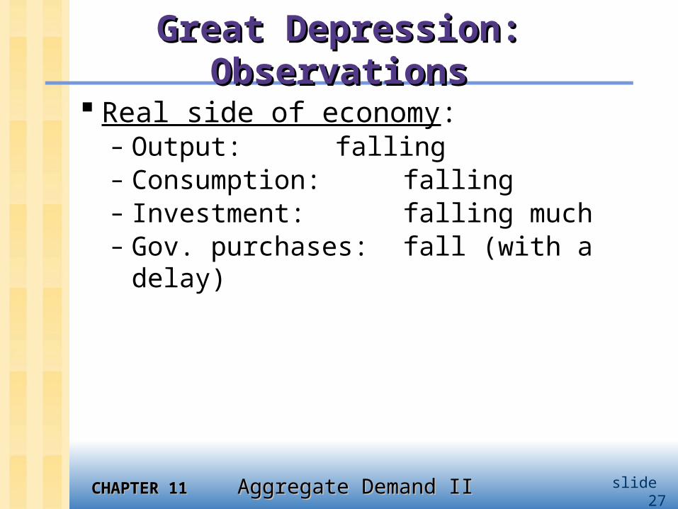
Great Depression: ObservationsGreat Depression: Observations

Real side of economy:– Output: falling– Consumption: falling– Investment: falling much– Gov. purchases: fall (with a

delay)



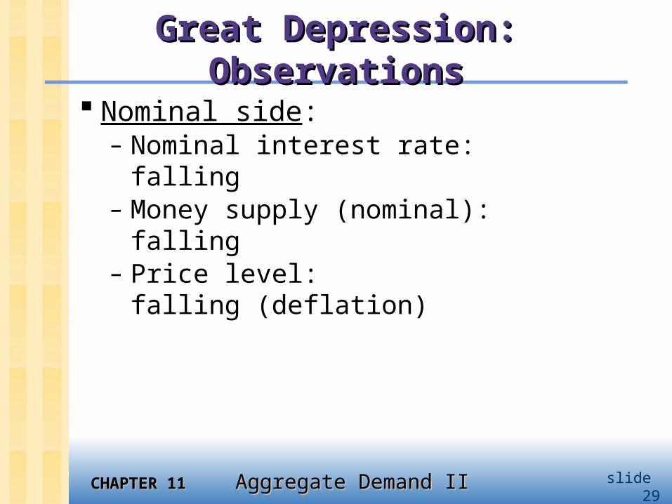
Great Depression: ObservationsGreat Depression: Observations

Nominal side:– Nominal interest rate: falling– Money supply (nominal): falling– Price level: falling

(deflation)


The Spending Hypothesis: The Spending Hypothesis: Shocks to the IS CurveShocks to the IS Curve

asserts that the Depression was largely due to an exogenous fall in the demand for goods & services -- a leftward shift of the IS curve

evidence: output and interest rates both fell, which is what a leftward IS shift would cause


The Spending Hypothesis: The Spending Hypothesis: Reasons for the IS shiftReasons for the IS shift

1. Stock market crash exogenous C Oct-Dec 1929: S&P 500 fell 17% Oct 1929-Dec 1933: S&P 500 fell 71%

2. Drop in investment “correction” after overbuilding in the

1920s widespread bank failures made it harder to

obtain financing for investment

3. Contractionary fiscal policy in the face of falling tax revenues and

increasing deficits, politicians raised tax rates and cut spending


The Money Hypothesis: The Money Hypothesis: A Shock to the LM CurveA Shock to the LM Curve

asserts that the Depression was largely due to huge fall in the money supply

evidence: M1 fell 25% during 1929-33.

But, two problems with this hypothesis:1. P fell even more, so M/P actually rose

slightly during 1929-31. 2. nominal interest rates fell, which is the

opposite of what would result from a leftward LM shift.


A revision to the Money HypothesisA revision to the Money Hypothesis

There was a big deflation: P fell 25% 1929-33.

A sudden fall in expected inflation means the ex-ante real interest rate rises for any given nominal rate (i)

ex ante real interest rate = i – e

This could have discouraged the investment expenditure and helped cause the depression.

Since the deflation likely was caused by fall in M, monetary policy may have played a role here.


Chapter summaryChapter summary

1. IS-LM model

a theory of aggregate demand

exogenous: M, G, T, P exogenous in short run, Y in long run

endogenous: r, Y endogenous in short run, P in long run

IS curve: goods market equilibrium

LM curve: money market equilibrium


Chapter summaryChapter summary

2. AD curve

shows relation between P and the IS-LM

model’s equilibrium Y.

negative slope because P (M/P ) r I Y

expansionary fiscal policy shifts IS curve right, raises income, and shifts AD curve right

expansionary monetary policy shifts LM

curve right, raises income, and shifts AD

curve right IS or LM shocks shift the AD curve


EXERCISE:EXERCISE: Analyze SR & LR effects of Analyze SR & LR effects of MM

a.Drawing the IS-LM and AD-AS diagrams as shown here,

b.show the short run effect of a Fed increases in M. Label points and show curve shifts with arrows.

c. Show what happens in the transition from the short run to the long run. Label points.

d.How do the new long-run equilibrium values compare to their initial values?

Y

r

Y

P LRAS

Y

LRAS

Y

IS

SRAS1P1

LM(M1/P1)

AD1


EXERCISE:EXERCISE: Short run Short run

Y

r

Y

P LRAS

Y

LRAS

Y

IS

SRAS1P1

LM(M1/P1)

AD1

LM(M2/P1)

AD2

Short run:

Rise in M raises real money

supply in money market

and shifts LM curve right.

Also shifts AD curve right.

Equilibrium moves from

point 0 to point 1.

Output rises to Y1.

Note that interest rate

falls from r0 to r1.

Y1

Y1

r1

r0

10

01


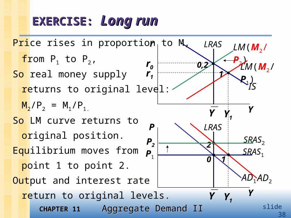
EXERCISE:EXERCISE: Long run Long run

Y

r

Y

P LRAS

Y

LRAS

Y

IS

SRAS1P1

LM(M2/P2)

AD1

LM(M2/P1)

AD2

Price rises in proportion to M,

from P1 to P2,

So real money supply

returns to original level:

M2/P2 = M1/P1.

So LM curve returns to

original position.

Equilibrium moves from

point 1 to point 2.

Output and interest rate

return to original levels.

Y1

Y1

r1

r0 0,2

2

1

1

0

SRAS2P2

Documents

Eva Hromadkova PowerPoint ® Slides by Ron Cronovich CHAPTER ELEVEN Aggregate Demand II macro © 2002 Worth Publishers, all rights reserved Topic 12a: Aggregate