Embed Size (px)
Citation preview
NBER WORKING PAPER SERIES
AFTER THE PANIC:ARE FINANCIAL CRISES DEMAND OR SUPPLY SHOCKS?
EVIDENCE FROM INTERNATIONAL TRADE
Felipe BenguriaAlan M. Taylor
Working Paper 25790http://www.nber.org/papers/w25790
NATIONAL BUREAU OF ECONOMIC RESEARCH1050 Massachusetts Avenue
Cambridge, MA 02138April 2019
This work was kindly supported by a research grant from The Bankard Fund for Political Economy at the University of Virginia. We benefitted from helpful comments from conference participants at the 2017 NBER Summer Institute. We are especially thankful to our discussant Julian di Giovanni. All errors are our own. The views expressed herein are those of the authors and do not necessarily reflect the views of the National Bureau of Economic Research.
At least one co-author has disclosed a financial relationship of potential relevance for this research. Further information is available online at http://www.nber.org/papers/w25790.ack
NBER working papers are circulated for discussion and comment purposes. They have not been peer-reviewed or been subject to the review by the NBER Board of Directors that accompanies official NBER publications.
© 2019 by Felipe Benguria and Alan M. Taylor. All rights reserved. Short sections of text, not to exceed two paragraphs, may be quoted without explicit permission provided that full credit, including © notice, is given to the source.
After the Panic: Are Financial Crises Demand or Supply Shocks? Evidence from InternationalTradeFelipe Benguria and Alan M. TaylorNBER Working Paper No. 25790April 2019JEL No. E44,F32,F36,F41,G01,N10,N20
ABSTRACT
Are financial crises a negative shock to demand or a negative shock to supply? This is a fundamental question for both macroeconomics researchers and those involved in real-time policymaking, and in both cases the question has become much more urgent in the aftermath of the recent financial crisis. Arguments for monetary and fiscal stimulus usually interpret such events as demand-side shortfalls. Conversely, arguments for tax cuts and structural reform often proceed from supply-side frictions. Resolving the question requires models capable of admitting both mechanisms, and empirical tests that can tell them apart. We develop a simple small open economy model, where a country is subject to deleveraging shocks that impose binding credit constraints on households and/or firms. These financial crisis events leave distinct statistical signatures in the empirical time series record, and they divide sharply between each type of shock. Household deleveraging shocks are mainly demand shocks, contract imports, leave exports largely unchanged, and depreciate the real exchange rate. Firm deleveraging shocks are mainly supply shocks, contract exports, leave imports largely unchanged, and appreciate the real exchange rate. To test these predictions, we compile the largest possible crossed dataset of 200+ years of trade flow data and event dates for almost 200 financial crises in a wide sample of countries. Empirical analysis reveals a clear picture: after a financial crisis event we find the dominant pattern to be that imports contract, exports hold steady or even rise, and the real exchange rate depreciates. History shows that, on average, financial crises are very clearly a negative shock to demand.
Felipe BenguriaDepartment of EconomicsGatton College of Business and EconomicsUniversity of Kentucky550 S LimestoneLexington, KY [email protected]
Alan M. TaylorDepartment of Economics andGraduate School of ManagementUniversity of CaliforniaOne Shields AveDavis, CA 95616-8578and CEPRand also [email protected]
1. Introduction
What is the link between financial crises and trade collapses, and what can macroeconomistslearn from it? In this paper we look to the past, exploring evidence from up to 200 years ofinternational trade and price data to answer this question. Our historical long-run approachis unique, differs from existing studies, and opens up potential new avenues for research.
In particular, we want to ask a very general question: are financial crises, on average,associated with a negative shock to demand or a negative shock to supply? This is animportant question to answer, because it can help guide better policy responses to futurefinancial crises. Arguably, had we known more in 2008, it might have made for a cleareranswer as to what was to blame for the Great Recession, and, thus, helped in the searchfor effective policy responses. In real time, clarity was lacking: many economists andpolicymakers sided with a demand shock explanation, but others argued the problem wason the supply side. Yet there were few evidence-based arguments based on similar eventsin the past. We show that the historical record might have cast some light and cut throughthe intellectual and political fog.
In the first part of our paper we develop a simple small open economy model, wherethe home country is subject to deleveraging shocks. The new theoretical contribution isthat these shocks can impose binding credit constraints either on households or on firms,or both. Our model builds on the work of Eggertsson and Krugman (2012)—in whichhouseholds adjust to sudden deleveraging shocks—by adding an analogous shock to firmsand by extending the framework to an open economy setting including a nontradable sectorand an endogenous real exchange rate. In the simulations of the model, we treat financialcrisis events as household or firm deleveraging shocks, and ask what kind of statisticalsignatures each kind of event would leave in the empirical time series record.
The answers are very clear, and divide sharply between each type of shock. Householddeleveraging shocks, setting aside second order equilibrium effects, are pure demandshocks; these will tend to contract imports, leave exports largely unchanged, and depreciatethe real exchange rate. Firm deleveraging shocks, setting aside second order equilibriumeffects, are pure supply shocks; these will tend to contract exports, leave imports largelyunchanged, and appreciate the real exchange rate. These clear contrasts in the modelpredictions help us take the theory to the data.
In the second part of our paper we present our empirical evidence. The rationale for along time frame is that financial crises are relatively rare events. To say anything meaningfulfrom a statistical standpoint, we must expand our data across countries, and back in time,as recent research has shown (Reinhart and Rogoff, 2009, 2011; Schularick and Taylor, 2012).
1
Our analysis centers on a substantial effort to assemble a new large historical dataset.In particular we extend and then match two types of datasets, historical bilateral data ontrade flows, and country-specific data on macroeconomic aggregates and financial crisisdates. With that done, we can look over a universe of almost 200 financial crises, and useempirical methods to get a clearer picture of how financial distress typically affects trade.
What does history show? When we look at the long-run trade and price data, matchthem with established financial crisis timings, and trace out the high frequency responses,do we find that financial crises exhibit the symptoms of demand shocks or supply shocks?The answer will turn out to be strikingly unambiguous.
Very clearly, after a financial crisis event we see statistical evidence strongly in favor ofthe demand-side view: on impact, imports contract, exports hold steady or even rise, andthe real exchange rate depreciates. All effects are statistically significant, and especially soin the bilateral data where the sample size exceeds 150,000 country pair-year observationsfor trade flows and real exchange rates. The effects persist out to a five year horizon.
Our results form part of an emerging view that household debt and deleveraging cyclesplay a highly influential role in economic fluctuations (Jorda, Schularick, and Taylor, 2013;Mian, Sufi, and Verner, 2017), but one novel contribution here is to bring evidence oninternational adjustment into the debate as an extra tool for validation.
We also dig deeper than just a single aggregate response. In both theory and empirics,rather than study only the effects on final goods, we further distinguish between tradein final goods and trade in intermediate inputs. In our model, household deleveragingshocks reduce the demand for imported final goods. In addition, households demandfewer non-traded goods, which causes firms to import fewer intermediate inputs. In thecase of firm deleveraging shocks, which limit production, imports of intermediate inputsfall, whereas imports of final goods are largely stable. We construct data on trade flows byproduct type for the post-WW2 period, and find that financial crises depress imports ofboth final and intermediate goods, providing further empirical evidence consistent withthe demand-side view of crises.
Our empirical results are quite stable across developed and developing countries, withthe difference that the decline in imports is deeper following financial crises in the latter.Since our data spans two centuries, we also ask whether financial crises in different erashave had different consequences over time. The answer is no; while we lose some precisionin our pre-WW2 estimates, in part due to a smaller sample size, qualitatively the responseof trade flows and prices is fairly stable across different eras.
In addition, though we initially treat financial crises as exogenous events, we later allowfor the possibility that these are endogenous to macroeconomic conditions. Following Jorda,
2
Schularick, and Taylor (2011) and Jorda, Schularick, and Taylor (2016) we use the method ofinverse propensity-score weighting to address the problem of bias arising from selection onobservables. Following Jorda, Schularick, and Taylor (2011) we use pre-crisis credit growthas a predictor of financial crises in our first stage. Reassuringly, all of our results remainvalid when we model crises as endogenous events in this way.
We also acknowledge that economies are exposed to various types of crises in additionto financial ones. Consequently, we extend our dataset with the dates of currency andinflation crises, stock market crises, and external and domestic sovereign debt crises, relyingon the benchmark timings provided by Reinhart and Rogoff (2011). Our results are robustto jointly controlling for all these other kinds of crises.
Gaps in our knowledge exposed by the recent crisis have encouraged a return toeconomic history to evaluate broad questions using a larger universe of data, allowing us toaccumulate better evidence on how crises affect the macroeconomy. In this paper, we findthat clearly, over the long sweep of history, the dominant effects of a financial crisis eventhave corresponded to the theoretical predictions of a demand shock, not a supply shock, asjudged by the evidence left in the time series data for trade flows and real exchange rates.
1.1. Contribution to the Literature
Our focus on trade takes off from an emerging literature following the 2008 financial crisis.A wave of studies attests to the interest in the study of the repercussion of financial crisesfor exports and imports in an open economy. Most of this work seeks to establish thereasons behind the observed collapse of international trade. Some have focused on directfinancial effects on certain sectors or firms (Chor and Manova, 2012; Amiti and Weinstein,2011; Iacovone and Zavacka, 2009; Abiad, Mishra, and Topalova, 2014).1
Another suggestion is that international trade in inputs is subject to greater fixedcosts of shipments; fixed costs induce periodic ordering, but wait-and-see might postponetrades when a supply shock hits the input importer (Alessandria, Kaboski, and Midrigan,2010). Part of the trade collapse could be a composition effect, since international trade isdominated so much by durable goods and intermediate inputs, and these are much more
1Two papers examine the response of trade flows to crises over the past recent decades. Iacovone andZavacka (2009) study the response of exports to credit conditions in 23 crises episodes during 1980–2006.Abiad, Mishra, and Topalova (2014) study the impact of both financial and sovereign debt crises during1970–2009 on imports and exports, finding that crises primarily depress imports. Our approach builds onbut differs substantially from this work. The main difference is in our goal. Our empirical findings and ourmodel work together to answer the key question in our paper: are financial crises demand or supply shocks?Second, we expand the time horizon fivefold. As argued earlier, we study only large financial crises whichare rare events. In addition, we focus not only on international trade flows but also on prices to distinguishthe demand versus supply shock explanations.
3

cyclical than GDP itself (Levchenko, Lewis, and Tesar, 2010; Eaton, Kortum, Neiman, andRomalis, 2016; Behrens, Corcos, and Mion, 2013; Bussiere, Callegari, Ghironi, Sestieri, andYamano, 2013). Finally, increases in uncertainty, often associated with financial crisis events,may trigger a disproportionate decline in imports relative to domestic non-traded activitydue to the interplay between the fixed costs of trade and the option value of waiting toplace an order for shipment (Novy and Taylor, 2014).2
These and other explanations may or may not be shown to be mutually exclusive inthe end. Our contribution to this literature is to develop a simple model that admits bothdemand and supply shocks and provides very clear, distinct predictions for the responsesof international trade flows and prices under each type of shock. Our theory departs fromstandard trade models by adapting recent intertemporal models of deleveraging shocksto an open economy setting. Our model’s predictions can be told apart very cleanly uponexamining the data. Our interest is not in the response of the economy to a single crisisepisode but in the average response to nearly 200 episodes over the past two centuries.
This paper also contributes to a literature documenting the causes and consequencesof financial crises (Reinhart, 2010; Reinhart and Rogoff, 2011; Schularick and Taylor, 2012;Jorda, Schularick, and Taylor, 2011). In the same spirit that motivates our paper, thiswork has looked at the past, gathering evidence from many financial crisis episodes overseveral decades or centuries. These papers have examined the impact of crises on severalmacroeconomic outcomes, such as GDP and unemployment, but not on international tradeflows and prices. Much of this literature focuses on documenting the consequences, not thecauses, of financial crises. Work that does ask for causes (such as Schularick and Taylor,2012) points to the role of credit, but does not seek to answer whether these events shouldbe understood as demand or supply shocks.
Finally, our work contributes to the recent and growing literature that examines, fromvarious perspectives, the causes of the recent Great Recession. In particular, Mian, Rao, andSufi (2013) find a large contraction in household spending in the U.S. as a consequenceof declining housing net worth; Mian and Sufi (2014) establish that this led in turn to alarge decline in employment; Mian, Sufi, and Verner (2017) provide global evidence ofthe same character. These and other findings based on recent data are consistent with thedemand-side view that our long-run historical evidence strongly support.
2These and other explanations are gathered in Baldwin (2009). Further empirical work on crises and tradeincludes Freund (2009) who examines the response of trade to global downturns; and Bems, Johnson, and Yi(2011) who study the role of vertical linkages in amplifying the trade collapse.
4
2. A Crisis-Deleveraging Model: Demand, Supply, and Trade Shocks
We study a small open economy and introduce borrowing limits into both the firm andhousehold side of the economy. This is guided by our desire to understand whether themacroeconomic effects of financial crises can be best understood as demand or supplyshocks. In the case of households, this apparatus exactly mirrors the approach of Eggertssonand Krugman (2012).3 We add the same apparatus to the firm side of the model to makeour modeling of the two shocks conceptually as simple and symmetric as possible.
Formally, we will describe an economy populated by patient and impatient households.These households derive utility from the consumption of an import good and a non-tradedgood. Firms in the economy produce a non-traded good sold locally and an export goodsold abroad. They produce using labor and imported inputs and must borrow to financea share of their production cost in advance. Both impatient households and firms faceexogenous, binding borrowing limits, and we study the impact on the economy of suddendeclines in the amount that households or firms can borrow.
2.1. Households
We assume that households maximize lifetime utility
U = E0
∞
∑t=0
(βi)t ·(
log(CiMt) + αN · log(Ci
Nt)−Ni1+φ
t1 + φ
),
subject to a budget constraint discussed below, with i ε{B, S} indexing borrowers and saversand time preference parameters such that βs > βb. We denote by Ci
M and CiN a household’s
consumption of the import good and the non-traded good, respectively. The householdbudget constraint supposes that they receive income as a wage for labor supplied to localfirms in the non-traded and export sectors. In addition, patient households (only) own andreceive firm profits.4
The economy faces an exogenous world price of the import good, PM, and an endoge-nously determined price of the non-traded good, PN . Households borrow from, or lend to,the rest of the world at an exogenous real interest rate r, subject to limits.
3In related work Benigno and Romei (2014) study how debt deleveraging in one country spreads to therest of the world economy.
4The assumption that only patient households receive firm profits is for analytical simplicity and followsMartinez and Philippon (2014).
5
We assume that the impatient households’ budget constraint is given by
PMt · CbMt + PN t · Cb
N t − Dbt = wt · Nb
t − (1 + rt−1) · Dbt−1 ,
and the binding borrowing constraint we impose on the impatient households is
(1 + rt) · Dbt ≤ D .
Similarly, we assume that the patient households’ budget constraint is given by
PMt · CsMt + PN t · Cs
N t − Dst = wt · Ns
t +πXt
χ+
πN t
χ− (1 + rt−1) · Ds
t−1 ,
where χ and 1− χ denote the fraction of patient and impatient households in the economy.
2.2. Production
We assume that in both the export and the non-traded sectors there is a continuum offirms of measure one that produce output using labor and imported inputs. Firms in theexport sector sell their goods to the rest of the world at the exogenous world price PX,while firms in the non-traded sector sell their good domestically at a price PN determinedin equilibrium. Inputs are traded at the exogenous world price PI .
In each sector, firms must borrow a fraction λ of their cost to finance production. Firmsborrow from the rest of the world at an exogenous real interest rate r, subject to limits.
We assume that in each sector S ε {N, X} the firms’ budget constraint is given by
πS t + δS t = δS t−1 · (1 + rt−1) + πS t ,
where δS t is the amount borrowed in period t, πS t denotes profits paid to households, andπS t denotes profits excluding the financing cost (revenue minus production cost). Whensimulating a firm deleveraging shock, we impose a binding limit δS on the amount firmscan borrow and that will be tightened suddenly by the shock.
Firms have the following generalized CES production function:
qS t =(θ · lρ
S t + (1− θ) · iρS t) ε
ρ ,
with ε < 1, which implies decreasing returns to scale.5
5Imposing decreasing returns to scale in the production function will allow both quantities and prices torespond to shocks.
6
Firms’ production cost is then given by CS t(qS t, wt, PI) =(
θσ · w1−σt + (1− θ)σ · P1−σ
I
) 11−σ ·
q1/ε
S t , with σ = 1/(1− ρ).In the absence of a binding borrowing constraint, firms—which are price takers—will
optimally produce at an output level qS t =(
ε · pS t/(
θσ · w1−σt + (1− θ)σ · P1−σ
I
) 11−σ
)ε/1− ε
, whileborrowing as necessary. However, at times when the borrowing constraint is presentand binding the firms will be restricted in the amount that they can produce. Firmsthen borrow λ · CS t = δS each period. This, in turn, implies that firms can only produceqS t =
(δS/
(λ ·(
θσ · w1−σt + (1− θ)σ · P1−σ
I
) 11−σ
))ε.
2.3. Equilibrium
In equilibrium the non-traded goods market clears, determining its price PN, where thecondition for demand equals supply is given by
χ · csN t + (1− χ) · cb
N t = qN t .
Finally, we assume wages evolve according to the following Phillips curve,
wt = wt−1 · (1 + κ · (Nt − Nss)) .
This assumption follows Martinez and Philippon (2014). We denote by Nss the steady statelevel of aggregate hours. The parameter κ regulates the speed of adjustment of wages,which is proportional to the deviation of aggregate hours from steady state. Wages aresticky, but in the limit κ → ∞ the economy converges to one with flexible wages. Understicky wages, shocks can lead to an excess supply of labor (unemployment) in which theequilibrium is demand-determined. Following Martinez and Philippon (2014) we rationthe labor market uniformly between the patient and impatient households.
2.4. Calibration
A first set of parameters is chosen directly based on the literature. Following Eggertssonand Krugman (2012) and Martin and Philippon (2017) we assume half the households areconstrained (χ = 0.5). We assign a value 0.04 to the real interest rate, and set the discountfactor of patient households such that βs = 1/(1 + r). We set the slope of the Phillips curveκ = 0.1 and the inverse elasticity of labor supply φ is set to 1 as in Monacelli (2009). Weassume the fraction of firms’ cost that must be financed before production takes place λ isset to 1/3. We assume values for the parameters of the production function ρ = 0.5, θ = 0.7,
7
and ε = 0.5, and we verify that simulation results do not change significantly as theseparameters vary.
The remaining parameters are the price of the export good (PX), the price of the importgood (PM), the price of the imported input (PI), the relative weight of the nontraded goodin the utility function (αN), and the borrowing limit for impatient households (D). Theseparameters are set to target the following conditions in the initial steady-state. First, weset the trade balance equal to zero, the share of inputs in total imports equal to either 10%or 40%, and the price of the import good and the export good equal.6 Second, we set theemployment share of the nontraded sector to either 60% or 80% of employment.7 Third, weset the debt to income ratio of impatient households equal to one, an assumption whichfollows Eggertsson and Krugman (2012).
Finally, in each sector the borrowing limit for firms (δS) is set to be just below theoptimal amount borrowed in the unrestricted steady state.
2.5. Simulations
The goal of the model is to permit us to simulate the responses of the economy to delever-aging shocks to households and firms.
Demand shock We interpret a decline in the borrowing limit for impatient households asa demand shock.8 All else equal, such households are forced to spend less on consumption,given their reduced ability to borrow. On impact, they reduce their consumption as theyborrow a now lower amount but still repay a higher amount borrowed in the previousperiod. This reduces demand for both the imported final good and the non-traded good,leading to lower aggregate demand. In response, the price of the non-traded good falls.Firms in the non-traded sector adjust their production, lowering their demand for theintermediate input. Lower demand for both the imported final good and the intermediateinput leads to lower imports. Exports vary only due to general equilibrium effects, asworld demand is unchanged. We simulate the response to two types of shocks to impatienthouseholds’ borrowing limit.
Figure 1 graphs the adjustment of exports, imports of the final good, the intermediateinput, and total imports, the trade balance, and the price of the non-traded good in responseto each of these shocks. The first shock, shown in panel A, is an unanticipated permanent
6While we do not have accurate historical data informing an average value of the share of imported inputsin total imports over our sample period, we believe these two values represent a reasonable range.
7Again, we do not have historical data describing the size of the nontradable sector, so we use a reasonablerange of parameters.
8When simulating this household deleveraging shock, we allow firms to borrow freely.
8
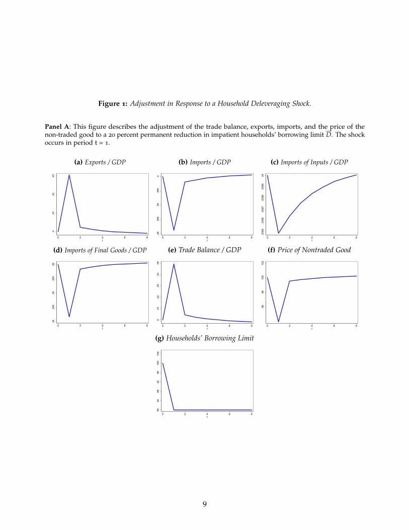
Figure 1: Adjustment in Response to a Household Deleveraging Shock.
Panel A: This figure describes the adjustment of the trade balance, exports, imports, and the price of thenon-traded good to a 20 percent permanent reduction in impatient households’ borrowing limit D. The shockoccurs in period t = 1.
(a) Exports / GDP
.4.4
1.4
2.4
3
0 2 4 6 8t
(b) Imports / GDP.3
8.3
85.3
9.3
95.4
0 2 4 6 8t
(c) Imports of Inputs / GDP
.039
5.0
396
.039
7.0
398
.039
9.0
4
0 2 4 6 8t
(d) Imports of Final Goods / GDP
.34
.345
.35
.355
.36
0 2 4 6 8t
(e) Trade Balance / GDP
0.0
1.0
2.0
3.0
4.0
5
0 2 4 6 8t
(f) Price of Nontraded Good96
9810
010
2
0 2 4 6 8t
(g) Households’ Borrowing Limit
8084
8892
9610
010
4
0 2 4 6 8t
9
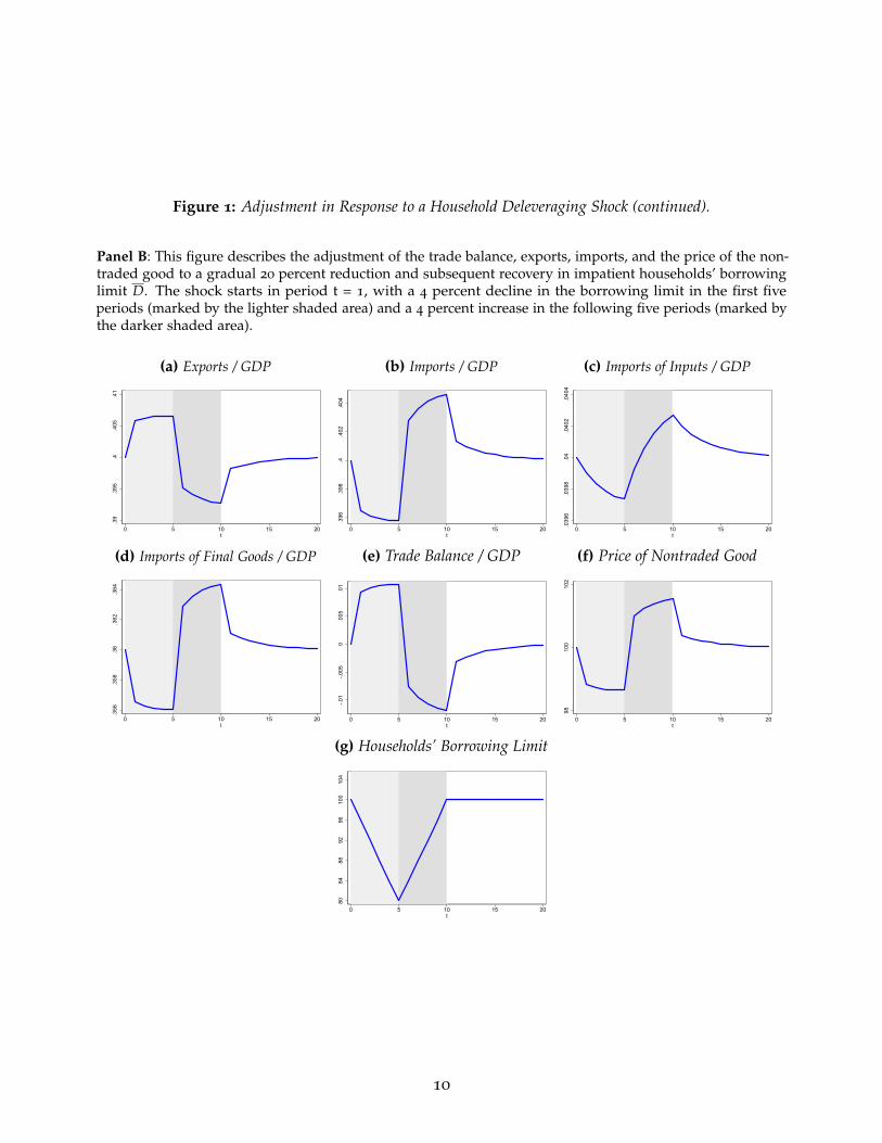
Figure 1: Adjustment in Response to a Household Deleveraging Shock (continued).
Panel B: This figure describes the adjustment of the trade balance, exports, imports, and the price of the non-traded good to a gradual 20 percent reduction and subsequent recovery in impatient households’ borrowinglimit D. The shock starts in period t = 1, with a 4 percent decline in the borrowing limit in the first fiveperiods (marked by the lighter shaded area) and a 4 percent increase in the following five periods (marked bythe darker shaded area).
(a) Exports / GDP
.39
.395
.4.4
05.4
1
0 5 10 15 20t
(b) Imports / GDP
.396
.398
.4.4
02.4
04
0 5 10 15 20t
(c) Imports of Inputs / GDP
.039
6.0
398
.04
.040
2.0
404
0 5 10 15 20t
(d) Imports of Final Goods / GDP
.356
.358
.36
.362
.364
0 5 10 15 20t
(e) Trade Balance / GDP
-.01
-.005
0.0
05.0
1
0 5 10 15 20t
(f) Price of Nontraded Good98
100
102
0 5 10 15 20t
(g) Households’ Borrowing Limit
8084
8892
9610
010
4
0 5 10 15 20t
10
decline in the borrowing limit. Given the fall in GDP, the ratio of exports to GDP rises whileimports to GDP fall, as imports fall further than GDP. Imports of both the final good andthe intermediate input fall. The trade balance rises in response to the decline in imports.The price of the non-traded good falls.
The second shock, in panel B of Figure 1, is an unanticipated gradual decline and subse-quent recovery in the borrowing limit, representing a more realistic multi-year financialcrisis. This generates similar paths for exports, imports and the price of the non-tradedgood during the decline in the borrowing limit. All these series, however, recover and“overshoot” beyond the initial level as the borrowing limit returns to the original. Thereason is that as the borrowing limit falls, constrained households are re-paying higherlevels of past (one-period) debt than they can currently borrow (i.e., refinance), whichreduces their consumption. But as the borrowing limit increases, the opposite happens,leading to an increase in their consumption.
Supply shock In turn, we interpret a decline in the borrowing limit for firms as a supplyshock. All else equal, every firm is forced to produce less output from less input, given theirreduced ability to borrow.
The immediate impact is to reduce the production of both the export good and thenon-traded good, as firms in both sectors face a tighter borrowing constraint. Exports falldirectly due to the shock. Further, the price of the non-traded good rises due to a decline insupply. A lower amount of credit to produce leads to a lower demand for the importedinput by both the export and the non-traded sectors. The shock also lowers wages andfirm profits in both sectors. This leads to lower income to both patient and impatienthouseholds. Patient households are able to smooth the impact of the shock over time, witha minor decline in demand, but impatient households cannot borrow and translate theirlower income fully into lower consumption. The ratio of imports of final goods to GDPrises as the fall in GDP is larger than the fall in imports. Total imports to GDP rise, as therise in final goods to GDP dominates the decline in imported inputs to GDP.
Figure 2 illustrates the adjustment in response to this type of shock. As before, wesimulate the economy’s adjustment to both an unanticipated permanent decline in thefirms’ borrowing limit (in panel A) and an unanticipated gradual decline and subsequentrecovery in the borrowing limit (in panel B). As with the shock to households, the gradualfirm deleveraging shock in panel B generates an “overshooting” in all outcomes.
Robustness We analyze these simulations varying two important steady-state ratios usedto calibrate the model’s parameters: the share of imported intermediate inputs in totalimports and the size (employment share) of the nontradable sector. As we show and
11
discuss in detail in Appendix B, our results are robust to using a wide range of calibratedparameters.
3. Data: Trade and Financial Crises over Two Centuries
The dataset used in this paper includes 69 developed and developing countries and coversthe period 1816–2014. We combine bilateral trade flows between all country pairs with dataon financial crises, GDP, and bilateral real exchange rates. We have also included in thedataset information on bilateral trade barriers as used in typical gravity models of trade.Our dataset is assembled gathering several data sources which we describe below.
3.1. Financial Crisis Dates
We rely on data on the dates of financial (i.e., banking) crises compiled by Reinhart andRogoff (2011). They define banking crises as episodes where bank runs lead to the publicsector assuming control of financial institutions, and/or episodes of large-scale financialassistance from the govermnment to financial institutions. These data are available for 70
countries.9,10 Reinhart and Rogoff (2011) mark financial crisis dates using dummy variablesat an annual frequency. We identify the first year of a crisis as the relevant shock event. Weexclude crises adjacent to major world wars, or around which we lack trade data. We thuscan analyze a maximum of 195 crisis episodes in our historical window. In this sample, 77
crises take place in advanced countries and 118 in developing economies; 108 crises occurin the post-WW2 period and 87 in the pre-WW2 era.11 The distribution of the number ofcrisis episodes by country is such that the median country faces 3 crisis episodes duringthe full sample window 1816–2014. At the extremes, the country at the 10th percentile facesa single financial crisis episode, while the country at the 90th percentile faces 6 crises overthe two centuries. Figure A.1 in the Appendix illustrates the frequency of financial crisesby year.
3.2. Bilateral and Total Trade Flows
Bilateral trade data were obtained from the newly available CEPII TRADHIST databasefor the pre-WW2 period and entirely from the IMF’s Direction of Trade Statistics for the
9We exclude Taiwan from our sample due to a lack of recent trade and GDP data.10 Appendix Table A.1 reports the list of countries and the financial crises start dates.11We consider the following set of 14 countries to be advanced economies: Australia, Austria, Belgium,
Canada, Denmark, France, Germany, Japan, the Netherlands, Norway, Sweden, Switzerland, the UnitedKingdom and the United States.
12
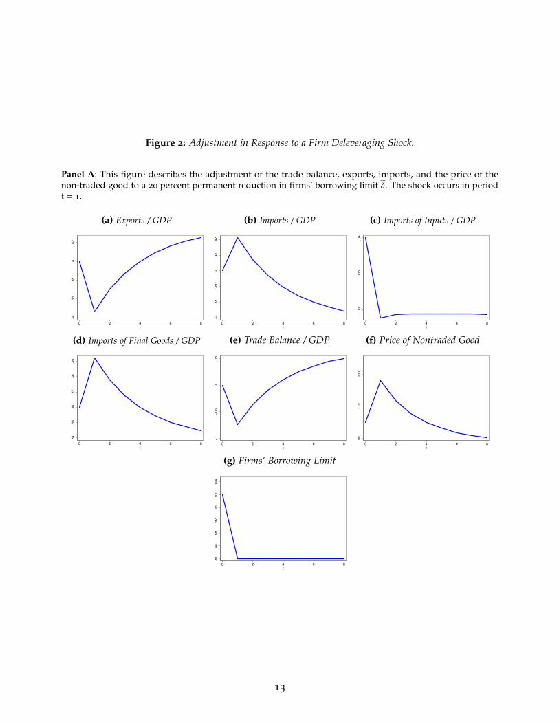
Figure 2: Adjustment in Response to a Firm Deleveraging Shock.
Panel A: This figure describes the adjustment of the trade balance, exports, imports, and the price of thenon-traded good to a 20 percent permanent reduction in firms’ borrowing limit δ. The shock occurs in periodt = 1.
(a) Exports / GDP
.34
.36
.38
.4.4
2
0 2 4 6 8t
(b) Imports / GDP.3
7.3
8.3
9.4
.41
.42
0 2 4 6 8t
(c) Imports of Inputs / GDP
.03
.035
.04
0 2 4 6 8t
(d) Imports of Final Goods / GDP
.34
.35
.36
.37
.38
.39
0 2 4 6 8t
(e) Trade Balance / GDP
-.1-.0
50
.05
0 2 4 6 8t
(f) Price of Nontraded Good
9011
013
0
0 2 4 6 8t
(g) Firms’ Borrowing Limit
8084
8892
9610
010
4
0 2 4 6 8t
13
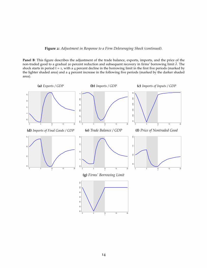
Figure 2: Adjustment in Response to a Firm Deleveraging Shock (continued).
Panel B: This figure describes the adjustment of the trade balance, exports, imports, and the price of thenon-traded good to a gradual 20 percent reduction and subsequent recovery in firms’ borrowing limit δ. Theshock starts in period t = 1, with a 4 percent decline in the borrowing limit in the first five periods (marked bythe lighter shaded area) and a 4 percent increase in the following five periods (marked by the darker shadedarea).
(a) Exports / GDP
.39
.4.4
1.4
2.4
3
0 5 10 15 20t
(b) Imports / GDP
.375
.38
.385
.39
.395
.4
0 5 10 15 20t
(c) Imports of Inputs / GDP
.03
.032
.034
.036
.038
.04
0 5 10 15 20t
(d) Imports of Final Goods / GDP
.34
.35
.36
.37
0 5 10 15 20t
(e) Trade Balance / GDP
-.02
0.0
2.0
4.0
6
0 5 10 15 20t
(f) Price of Nontraded Good90
100
110
120
0 5 10 15 20t
(g) Firms’ Borrowing Limit
8084
8892
9610
010
4
0 5 10 15 20t
14
post-WW2 period.12 Trade figures are reported in nominal U.S. dollars, which we deflateusing the U.S. GDP deflator.
We also assemble a second dataset on country-level total exports, total imports, GDP,and financial crises over the same period and sample of countries to provide more aggregateevidence on the response of trade following crises.
Trade in Final Goods and Intermediate Inputs We also construct a dataset of bilateraltrade flows by product type spanning the period 1962–2014. These data are restrictedto the post-WW2 period as product-level data are not systematically available for earlierdecades. Broadly, our procedure involves obtaining data by product, by year, and byexporter-importer pair from the United Nations’ COMTRADE database and assigning eachindividual product into final goods, intermediate inputs, or capital goods categories. Thecoding of products into these aggregate groups is standard and follows Hummels, Ishii,and Yi (2001).13 We exclude from our data fuels, which at times represent a relevant shareof world trade, and a small set of unmatched products.
3.3. GDP and Real Exchange Rates
Our historical GDP series are assembled from various sources. Whenever possible weobtain real GDP series from Glick and Taylor (2010) and from Maddison (1995, 2001). Inrecent years, we use the World Bank’s World Development Indicators database. To fill in gapsin the early years in our sample we also use Barro and Ursua (2008) and Mitchell (1992,1993, 1995).
We also construct measures of bilateral real exchange rates. We obtain nominal exchangerates from the IMF’s International Financial Statistics for the post-1950 period and from GlobalFinancial Data for the pre-WW2 period. We obtain series on price levels from Reinhart andRogoff (2011) for most of our sample, and from the IMF’s World Economic Outlook for veryrecent years.
3.4. World Trade and Major Crises
To motivate our analysis, we note that what was witnessed after the global financial crisisin 2008 was nothing new, especially not the so-called Great Trade Collapse, meaning the
12The CEPII TRADHIST project has extended substantially the amount of pre-WW2 data available in earlierdatasets, adding years further into the past and filling in many gaps. Existing research examining historicaltrade flows typically have a starting point of 1870. For details on the construction of see CEPII TRADHISTdatabase see Fouquin and Hugot (2016).
13We match SITC revision 1 product codes in COMTRADE to BEC codes used by Hummels, Ishii, and Yi(2001) using a concordance obtained from the United Nations’ Statistics Division.
15
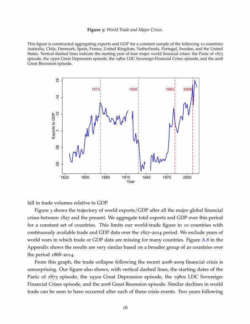
Figure 3: World Trade and Major Crises.
This figure is constructed aggregating exports and GDP for a constant sample of the following 10 countries:Australia, Chile, Denmark, Spain, France, United Kingdom, Netherlands, Portugal, Sweden, and the UnitedStates. Vertical dashed lines indicate the starting year of four major world financial crises: the Panic of 1873
episode, the 1930s Great Depression episode, the 1980s LDC Sovereign-Financial Crises episode, and the 2008
Great Recession episode.
1873 1928 1982 2008
.06
.08
.1.1
2.1
4.1
6E
xpor
ts to
GD
P
1820 1850 1880 1910 1940 1970 2000Year
fall in trade volumes relative to GDP.Figure 3 shows the trajectory of world exports/GDP after all the major global financial
crises between 1827 and the present. We aggregate total exports and GDP over this periodfor a constant set of countries. This limits our world-trade figure to 10 countries withcontinuously available trade and GDP data over the 1827–2014 period. We exclude years ofworld wars in which trade or GDP data are missing for many countries. Figure A.8 in theAppendix shows the results are very similar based on a broader group of 20 countries overthe period 1868–2014.
From this graph, the trade collapse following the recent 2008–2009 financial crisis isunsurprising. Our figure also shows, with vertical dashed lines, the starting dates of thePanic of 1873 episode, the 1930s Great Depression episode, the 1980s LDC Sovereign-Financial Crises episode, and the 2008 Great Recession episode. Similar declines in worldtrade can be seen to have occurred after each of these crisis events. Two years following
16
the start of the Great Recession in 2008, world exports to GDP in our data had fallen by0.93 percentage points. This is a similar decline to that in the early 1980s, when the trade toGDP fell ratio fell by 0.86 percentage points. The impact of the Great Depression, however,was almost twice as large, with a 1.45 percentage point fall in world trade to GDP.
However, the recovery of trade after the recent “trade collapse” was faster — comparedto output — than that seen in previous episodes. Five years following the start of the GreatRecession the exports-to-GDP ratio was 0.1 percentage points higher than in the year priorto the start of the crisis, while in the 1980s debt crisis and the Panic of 1873 it was still onepercentage point lower. The Great Depression stands out in this regard. Due perhaps torising protectionist measures adopted by the U.S. and other countries during this period(and other rising frictions, such as the collapse of the gold standard) exports-to-GDP werestill more than 3 percentage points lower than in the year prior to the start of the crisis.
This figure nicely motivates our study by revealing an enduring link between crisisevents and trade outcomes. What is obscured in this figure, however, is the uneven impactof financial crises on imports and exports, and the correlation between those shocks andthe location of the underlying financial frictions. The next sections focus on those issueswith a granular empirical analysis.
4. Response of Total Trade Flows to Financial Crises
Our first empirical exercise examines the evolution of countries’ aggregate exports andimports following financial crises in our historical 1816–2014 panel. We count 172 suchcrisis episodes, a third of which occur in the developed countries in our sample. Reinhartand Rogoff (2009) and Jorda, Schularick, and Taylor (2013), and others, have documentedthe deep impact of crisis episodes on various outcomes such as output, unemployment,and government debt, and the pace of recovery. With the same historical perspective, wewill focus on international trade.
Formally, let ln Tit denote a trade flow, which will be either total exports (Xit) or totalimports (Mit) for country i in year t, measured in real constant dollars. In the sameunits we also measure GDP, denoted Yit. Imposing a benchmark unit trade elasticity (i.e.,homotheticity, as in standard gravity models) with respect to country GDP, we study thesize-normalized trade flow ln(Tit/Yit). We are interested in the dynamic response of thisobject, in the aftermath of a financial crisis event in country i. Thus, we denote by Crisisit
the dummy variable which indicates the start of a financial crisis event. We then trace outthe response of the normalized trade flow from time t to time t + h across all episodes,using the local projection method of Jorda (2005) and estimating the series of regression for
17

each horizon h
ln(Ti,t+h/Yi,t+h)− ln(Tit/Yit) = αhi + βh
t + γhCrisisit + eit , (1)
where αhi are country fixed effects and βh
t are year fixed effects. The coefficient of interest isγh which denotes the response at horizon h to a financial crisis. These coefficients show how,controlling for pure GDP scaling effects, the financial crisis shock affects trade volumes. Theestimation is by OLS with standard errors clustered by pair and year, and all time-invariantcountry characteristics (e.g., certain geographical factors) are absorbed in the fixed effects.
Figure 4 and Table 1 show our estimates for the full sample. We find that on impact afinancial crisis is associated with a decrease in GDP-normalized imports (−4.9% change).14
But we find that on impact a financial crisis is associated with a (not statistically significant)increase in normalized exports. The effects on imports remain of a similar magnitude andstatistically significant even out to the horizon h = 5 years (−6.0% change), while the effecton exports remain not statistically different from zero.
Studies of the “trade collapse” during the recent Great Recession document similarpatterns and are motivated by the very large fall in trade in comparison to output. Becausethe 2008 event was a global crisis hitting many countries simultaneously, and because acountry’s exports are other countries’ imports, it is difficult to tell apart in this recent episodewhether the crisis depressed imports, exports, or both. Our empirical strategy can make thisdistinction, and the results show clearly that crises lower imports. A second message thatemerges is that large decline in imports relative to GDP are the norm historically. Finally,the historical record indicates that financial crises disrupt trade flows for many years.
We now turn to robstness. If we exclude the Great Recession, as in Figure 5a, the resultsare similar to those for the full sample. In the post-WW2 sample (shown in 5b), whichincludes 55% of the crisis episodes, the decline in imports relative to GDP is even largerthan in the full sample. On impact, the normalized trade flow declines −5.9% at a two-yearhorizon in the full sample and −8.9% in the post-WW2 era. In both cases, normalizedexports rise but the impact is not statistically significant. Our estimates for the pre-WW2
period (in Figure 5c) are blurrier. Imports still fall relative to GDP (−4.1% change) onimpact, but recover faster than in the full sample baseline. Normalized exports climbsusbtantially over time. In both cases, standard errors are wider, due perhaps primarily tothe smaller sample size.15
We also examine the response of exports and imports in developed and developing
14Strictly, the units of the estimated coefficients are log points, but for simplicity we refer to them using the% sign from here onwards as this is a close approximation.
15The estimated coefficients corresponding to Figure 5 are shown in Appendix Table A.2.
18
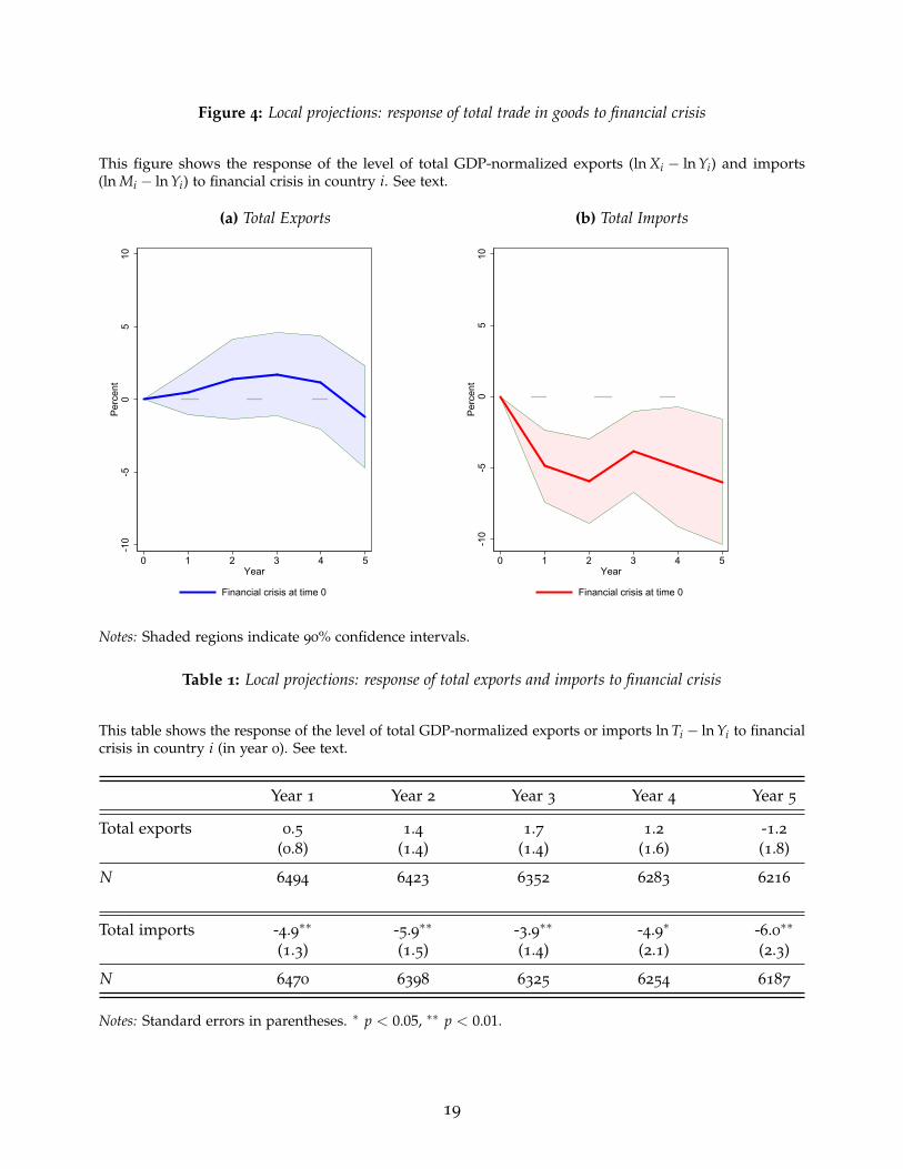
Figure 4: Local projections: response of total trade in goods to financial crisis
This figure shows the response of the level of total GDP-normalized exports (ln Xi − ln Yi) and imports(ln Mi − ln Yi) to financial crisis in country i. See text.
(a) Total Exports
-10
-50
510
Per
cent
0 1 2 3 4 5Year
Financial crisis at time 0
(b) Total Imports
-10
-50
510
Per
cent
0 1 2 3 4 5Year
Financial crisis at time 0
Notes: Shaded regions indicate 90% confidence intervals.
Table 1: Local projections: response of total exports and imports to financial crisis
This table shows the response of the level of total GDP-normalized exports or imports ln Ti − ln Yi to financialcrisis in country i (in year 0). See text.
Year 1 Year 2 Year 3 Year 4 Year 5
Total exports 0.5 1.4 1.7 1.2 -1.2(0.8) (1.4) (1.4) (1.6) (1.8)
N 6494 6423 6352 6283 6216
Total imports -4.9∗∗ -5.9∗∗ -3.9∗∗ -4.9∗ -6.0∗∗
(1.3) (1.5) (1.4) (2.1) (2.3)
N 6470 6398 6325 6254 6187
Notes: Standard errors in parentheses. ∗ p < 0.05, ∗∗ p < 0.01.
19
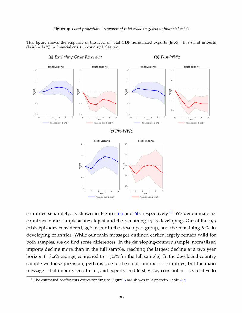
Figure 5: Local projections: response of total trade in goods to financial crisis
This figure shows the response of the level of total GDP-normalized exports (ln Xi − ln Yi) and imports(ln Mi − ln Yi) to financial crisis in country i. See text.
(a) Excluding Great Recession
-10
-50
510
Per
cent
0 1 2 3 4 5Year
Financial crisis at time 0
Total Exports
-10
-50
510
Per
cent
0 1 2 3 4 5Year
Financial crisis at time 0
Total Imports
(b) Post-WW2
-10
-50
510
Per
cent
0 1 2 3 4 5Year
Financial crisis at time 0
Total Exports
-10
-50
510
Per
cent
0 1 2 3 4 5Year
Financial crisis at time 0
Total Imports
(c) Pre-WW2
-10
-50
510
Per
cent
0 1 2 3 4 5Year
Financial crisis at time 0
Total Exports
-10
-50
510
Per
cent
0 1 2 3 4 5Year
Financial crisis at time 0
Total Imports
countries separately, as shown in Figures 6a and 6b, respectively.16 We denominate 14
countries in our sample as developed and the remaining 55 as developing. Out of the 195
crisis episodes considered, 39% occur in the developed group, and the remaining 61% indeveloping countries. While our main messages outlined earlier largely remain valid forboth samples, we do find some differences. In the developing-country sample, normalizedimports decline more than in the full sample, reaching the largest decline at a two yearhorizon (−8.2% change, compared to −5.9% for the full sample). In the developed-countrysample we loose precision, perhaps due to the small number of countries, but the mainmessage—that imports tend to fall, and exports tend to stay stay constant or rise, relative to
16The estimated coefficients corresponding to Figure 6 are shown in Appendix Table A.3.
20

Figure 6: Local projections: response of total trade in goods to financial crisis
This figure shows the response of the level of total GDP-normalized exports (ln Xi − ln Yi) and imports(ln Mi − ln Yi) to financial crisis in country i. See text.
(a) Advanced Economies - Full Sample
-10
-50
510
Per
cent
0 1 2 3 4 5Year
Financial crisis at time 0
Total Exports
-10
-50
510
Per
cent
0 1 2 3 4 5Year
Financial crisis at time 0
Total Imports
(b) Developing Economies - Full Sample
-10
-50
510
Per
cent
0 1 2 3 4 5Year
Financial crisis at time 0
Total Exports
-10
-50
510
Per
cent
0 1 2 3 4 5Year
Financial crisis at time 0
Total Imports
GDP—still stands.The results above appear inconsistent with the supply-side view of financial crises,
and consistent with the demand-side view of financial crises. However, up to now ourexamination of total trade flows does not take into account events in countries’ tradingpartners. In the next section we extend this approach to consider bilateral trade flows,sharpening our identification.
5. Response of Bilateral Trade Flows to Financial Crises
In this section we take our empirical work to the most granular level possible. We nowconsider all country pairs, in all years, and look at the post-crisis response of exports,imports, and also the real exchange rate, for every given pair-year observation. Not onlywill this greatly expand the number of observations, it will also allow us to more exactlycontrol for the incidence of financial crises potentially affecting one or both trading partnersin any given observation.
As a starting point, we treat crises as exogenous events. Later we will address reversecausality, that is, the concern that financial crisis episodes might be a “nonrandom treatment”which is endogenous to macroeconomic conditions.
In new notation for this setting, we now denote by Teit the trade flow from exportercountry e to importer country i in year t, and we denote by Yet and Yit the GDP level ineach country, all measured in real constant dollars. We construct the size-normalized trade
21
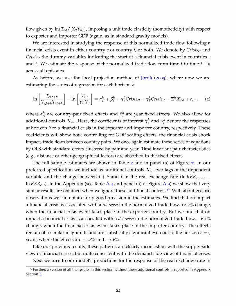
flow given by ln(Teit/[YetYit]), imposing a unit trade elasticity (homotheticity) with respectto exporter and importer GDP (again, as in standard gravity models).
We are interested in studying the response of this normalized trade flow following afinancial crisis event in either country e or country i, or both. We denote by Crisiset andCrisisit the dummy variables indicating the start of a financial crisis event in countries eand i. We estimate the response of the normalized trade flow from time t to time t + hacross all episodes.
As before, we use the local projection method of Jorda (2005), where now we areestimating the series of regression for each horizon h
ln[
Tei,t+h
Ye,t+hYi,t+h
]− ln
[Teit
YetYit
]= αh
ei + βht + γh
e Crisiset + γhi Crisisit + ΞhXeit + eeit , (2)
where αhei are country-pair fixed effects and βh
t are year fixed effects. We also allow foradditional controls Xeit. Here, the coefficients of interest γh
e and γhi denote the responses
at horizon h to a financial crisis in the exporter and importer country, respectively. Thesecoefficients will show how, controlling for GDP scaling effects, the financial crisis shockimpacts trade flows between country pairs. We once again estimate these series of equationsby OLS with standard errors clustered by pair and year. Time-invariant pair characteristics(e.g., distance or other geographical factors) are absorbed in the fixed effects.
The full sample estimates are shown in Table 2 and in panel (a) of Figure 7. In ourpreferred specification we include as additional controls Xeit two lags of the dependentvariable and the change between t + h and t in the real exchange rate (ln RERei,t+h −ln RERei,t). In the Appendix (see Table A.4 and panel (a) of Figure A.9) we show that verysimilar results are obtained when we ignore these additional controls.17 With about 200,000
observations we can obtain fairly good precision in the estimates. We find that on impacta financial crisis is associated with a increase in the normalized trade flow, +2.2% change,when the financial crisis event takes place in the exporter country. But we find that onimpact a financial crisis is associated with a decrease in the normalized trade flow, −6.1%change, when the financial crisis event takes place in the importer country. The effectsremain of a similar magnitude and are statistically significant even out to the horizon h = 5
years, where the effects are +3.2% and −4.6%.Like our previous results, these patterns are clearly inconsistent with the supply-side
view of financial crises, but quite consistent with the demand-side view of financial crises.Next we turn to our model’s predictions for the response of the real exchange rate in
17Further, a version of all the results in this section without these additional controls is reported in AppendixSection E.
22
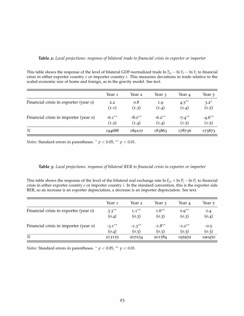
Table 2: Local projections: response of bilateral trade to financial crisis in exporter or importer
This table shows the response of the level of bilateral GDP-normalized trade ln Tei − ln Ye − ln Yi to financialcrisis in either exporter country e or importer country i. This measures deviations in trade relative to thescaled economic size of home and foreign, as in the gravity model. See text.
Year 1 Year 2 Year 3 Year 4 Year 5
Financial crisis in exporter (year 0) 2.2 0.8 1.9 4.5∗∗ 3.2∗
(1.1) (1.3) (1.4) (1.4) (1.5)
Financial crisis in importer (year 0) -6.1∗∗ -8.0∗∗ -6.2∗∗ -7.4∗∗ -4.6∗∗
(1.2) (1.4) (1.4) (1.5) (1.5)
N 194688 189107 183863 178736 173873
Notes: Standard errors in parentheses. ∗ p < 0.05, ∗∗ p < 0.01.
Table 3: Local projections: response of bilateral RER to financial crisis in exporter or importer
This table shows the response of the level of the bilateral real exchange rate ln Eei + ln Pi − ln Pe to financialcrisis in either exporter country e or importer country i. In the standard convention, this is the exporter sideRER, so an increase is an exporter depreciation, a decrease is an importer depreciation. See text.
Year 1 Year 2 Year 3 Year 4 Year 5
Financial crisis in exporter (year 0) 3.3∗∗ 1.1∗∗ 1.6∗∗ 0.9∗∗ 0.4(0.4) (0.3) (0.3) (0.3) (0.4)
Financial crisis in importer (year 0) -3.1∗∗ -1.3∗∗ -1.8∗∗ -1.0∗∗ -0.5(0.4) (0.3) (0.3) (0.3) (0.3)
N 213155 207234 201584 195952 190450
Notes: Standard errors in parentheses. ∗ p < 0.05, ∗∗ p < 0.01.
23
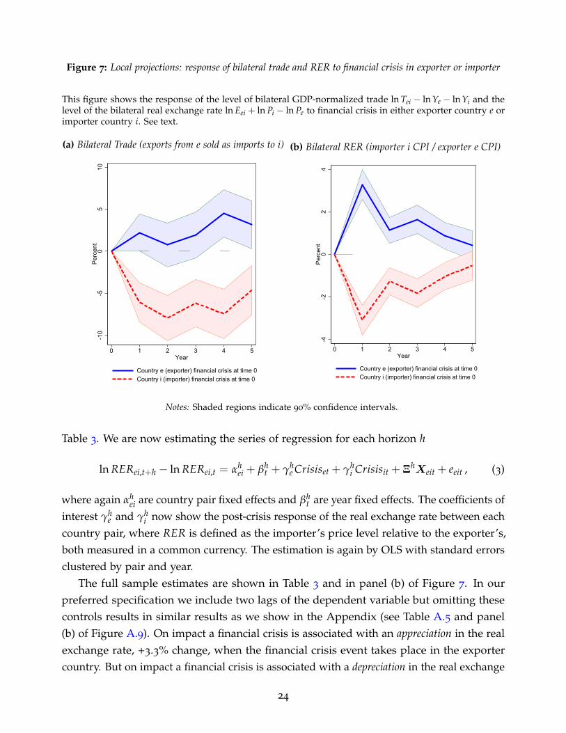
Figure 7: Local projections: response of bilateral trade and RER to financial crisis in exporter or importer
This figure shows the response of the level of bilateral GDP-normalized trade ln Tei − ln Ye − ln Yi and thelevel of the bilateral real exchange rate ln Eei + ln Pi − ln Pe to financial crisis in either exporter country e orimporter country i. See text.
(a) Bilateral Trade (exports from e sold as imports to i)
-10
-50
510
Per
cent
0 1 2 3 4 5Year
Country e (exporter) financial crisis at time 0Country i (importer) financial crisis at time 0
(b) Bilateral RER (importer i CPI / exporter e CPI)
-4-2
02
4P
erce
nt
0 1 2 3 4 5Year
Country e (exporter) financial crisis at time 0Country i (importer) financial crisis at time 0
Notes: Shaded regions indicate 90% confidence intervals.
Table 3. We are now estimating the series of regression for each horizon h
ln RERei,t+h − ln RERei,t = αhei + βh
t + γhe Crisiset + γh
i Crisisit + ΞhXeit + eeit , (3)
where again αhei are country pair fixed effects and βh
t are year fixed effects. The coefficients ofinterest γh
e and γhi now show the post-crisis response of the real exchange rate between each
country pair, where RER is defined as the importer’s price level relative to the exporter’s,both measured in a common currency. The estimation is again by OLS with standard errorsclustered by pair and year.
The full sample estimates are shown in Table 3 and in panel (b) of Figure 7. In ourpreferred specification we include two lags of the dependent variable but omitting thesecontrols results in similar results as we show in the Appendix (see Table A.5 and panel(b) of Figure A.9). On impact a financial crisis is associated with an appreciation in the realexchange rate, +3.3% change, when the financial crisis event takes place in the exportercountry. But on impact a financial crisis is associated with a depreciation in the real exchange
24
rate, −3.1% change, when the financial crisis event takes place in the importer country.Even at horizon h = 4 years, the effects are +0.9% and −1.0% and statistically significant.
Again, based on our model, the patterns are clearly inconsistent with the supply-sideview, but quite consistent with the demand-side view of financial crises.
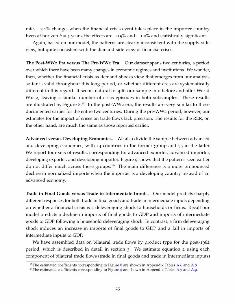
The Post-WW2 Era versus The Pre-WW2 Era. Our dataset spans two centuries, a periodover which there have been many changes in economic regimes and institutions. We wonder,then, whether the financial-crisis-as-demand-shocks view that emerges from our analysisso far is valid throughout this long period, or whether different eras are systematicallydifferent in this regard. It seems natural to split our sample into before and after WorldWar 2, leaving a similar number of crisis episodes in both subsamples. These resultsare illustrated by Figure 8.18 In the post-WW2 era, the results are very similar to thosedocumented earlier for the entire two centuries. During the pre-WW2 period, however, ourestimates for the impact of crises on trade flows lack precision. The results for the RER, onthe other hand, are much the same as those reported earlier.
Advanced versus Developing Economies. We also divide the sample between advancedand developing economies, with 14 countries in the former group and 55 in the latter.We report four sets of results, corresponding to: advanced exporter, advanced importer,developing exporter, and developing importer. Figure 9 shows that the patterns seen earlierdo not differ much across these groups.19 The main difference is a more pronounceddecline in normalized imports when the importer is a developing country instead of anadvanced economy.
Trade in Final Goods versus Trade in Intermediate Inputs. Our model predicts sharplydifferent responses for both trade in final goods and trade in intermediate inputs dependingon whether a financial crisis is a deleveraging shock to households or firms. Recall ourmodel predicts a decline in imports of final goods to GDP and imports of intermediategoods to GDP following a household deleveraging shock. In contrast, a firm deleveragingshock induces an increase in imports of final goods to GDP and a fall in imports ofintermediate inputs to GDP.
We have assembled data on bilateral trade flows by product type for the post-1962
period, which is described in detail in section 3. We estimate equation 2 using eachcomponent of bilateral trade flows (trade in final goods and trade in intermediate inputs)
18The estimated coefficients corresponding to Figure 8 are shown in Appendix Tables A.6 and A.8.19The estimated coefficients corresponding to Figure 9 are shown in Appendix Tables A.7 and A.9.
25
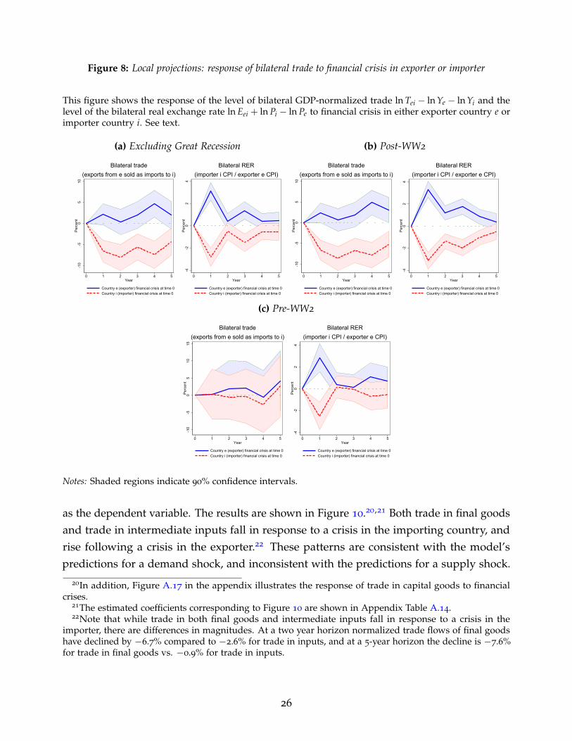
Figure 8: Local projections: response of bilateral trade to financial crisis in exporter or importer
This figure shows the response of the level of bilateral GDP-normalized trade ln Tei − ln Ye − ln Yi and thelevel of the bilateral real exchange rate ln Eei + ln Pi − ln Pe to financial crisis in either exporter country e orimporter country i. See text.
(a) Excluding Great Recession
-10
-50
510
Per
cent
0 1 2 3 4 5Year
Country e (exporter) financial crisis at time 0Country i (importer) financial crisis at time 0
Bilateral trade(exports from e sold as imports to i)
-4-2
02
4P
erce
nt
0 1 2 3 4 5Year
Country e (exporter) financial crisis at time 0Country i (importer) financial crisis at time 0
Bilateral RER(importer i CPI / exporter e CPI)
(b) Post-WW2
-10
-50
510
Per
cent
0 1 2 3 4 5Year
Country e (exporter) financial crisis at time 0Country i (importer) financial crisis at time 0
Bilateral trade(exports from e sold as imports to i)
-4-2
02
4P
erce
nt
0 1 2 3 4 5Year
Country e (exporter) financial crisis at time 0Country i (importer) financial crisis at time 0
Bilateral RER(importer i CPI / exporter e CPI)
(c) Pre-WW2
-10
-50
510
15P
erce
nt
0 1 2 3 4 5Year
Country e (exporter) financial crisis at time 0Country i (importer) financial crisis at time 0
Bilateral trade(exports from e sold as imports to i)
-4-2
02
4P
erce
nt
0 1 2 3 4 5Year
Country e (exporter) financial crisis at time 0Country i (importer) financial crisis at time 0
Bilateral RER(importer i CPI / exporter e CPI)
Notes: Shaded regions indicate 90% confidence intervals.
as the dependent variable. The results are shown in Figure 10.20,21 Both trade in final goodsand trade in intermediate inputs fall in response to a crisis in the importing country, andrise following a crisis in the exporter.22 These patterns are consistent with the model’spredictions for a demand shock, and inconsistent with the predictions for a supply shock.
20In addition, Figure A.17 in the appendix illustrates the response of trade in capital goods to financialcrises.
21The estimated coefficients corresponding to Figure 10 are shown in Appendix Table A.14.22Note that while trade in both final goods and intermediate inputs fall in response to a crisis in the
importer, there are differences in magnitudes. At a two year horizon normalized trade flows of final goodshave declined by −6.7% compared to −2.6% for trade in inputs, and at a 5-year horizon the decline is −7.6%for trade in final goods vs. −0.9% for trade in inputs.
26
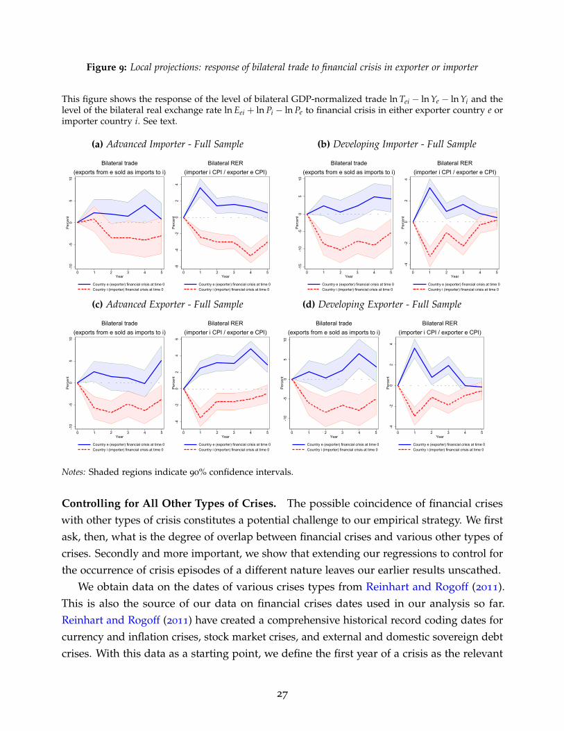
Figure 9: Local projections: response of bilateral trade to financial crisis in exporter or importer
This figure shows the response of the level of bilateral GDP-normalized trade ln Tei − ln Ye − ln Yi and thelevel of the bilateral real exchange rate ln Eei + ln Pi − ln Pe to financial crisis in either exporter country e orimporter country i. See text.
(a) Advanced Importer - Full Sample
-10
-50
510
Per
cent
0 1 2 3 4 5Year
Country e (exporter) financial crisis at time 0Country i (importer) financial crisis at time 0
Bilateral trade(exports from e sold as imports to i)
-6-4
-20
24
Per
cent
0 1 2 3 4 5Year
Country e (exporter) financial crisis at time 0Country i (importer) financial crisis at time 0
Bilateral RER(importer i CPI / exporter e CPI)
(b) Developing Importer - Full Sample
-15
-10
-50
510
Per
cent
0 1 2 3 4 5Year
Country e (exporter) financial crisis at time 0Country i (importer) financial crisis at time 0
Bilateral trade(exports from e sold as imports to i)
-4-2
02
4P
erce
nt
0 1 2 3 4 5Year
Country e (exporter) financial crisis at time 0Country i (importer) financial crisis at time 0
Bilateral RER(importer i CPI / exporter e CPI)
(c) Advanced Exporter - Full Sample
-10
-50
510
Per
cent
0 1 2 3 4 5Year
Country e (exporter) financial crisis at time 0Country i (importer) financial crisis at time 0
Bilateral trade(exports from e sold as imports to i)
-4-2
02
46
Per
cent
0 1 2 3 4 5Year
Country e (exporter) financial crisis at time 0Country i (importer) financial crisis at time 0
Bilateral RER(importer i CPI / exporter e CPI)
(d) Developing Exporter - Full Sample
-10
-50
510
Per
cent
0 1 2 3 4 5Year
Country e (exporter) financial crisis at time 0Country i (importer) financial crisis at time 0
Bilateral trade(exports from e sold as imports to i)
-4-2
02
4P
erce
nt
0 1 2 3 4 5Year
Country e (exporter) financial crisis at time 0Country i (importer) financial crisis at time 0
Bilateral RER(importer i CPI / exporter e CPI)
Notes: Shaded regions indicate 90% confidence intervals.
Controlling for All Other Types of Crises. The possible coincidence of financial criseswith other types of crisis constitutes a potential challenge to our empirical strategy. We firstask, then, what is the degree of overlap between financial crises and various other types ofcrises. Secondly and more important, we show that extending our regressions to control forthe occurrence of crisis episodes of a different nature leaves our earlier results unscathed.
We obtain data on the dates of various crises types from Reinhart and Rogoff (2011).This is also the source of our data on financial crises dates used in our analysis so far.Reinhart and Rogoff (2011) have created a comprehensive historical record coding dates forcurrency and inflation crises, stock market crises, and external and domestic sovereign debtcrises. With this data as a starting point, we define the first year of a crisis as the relevant
27
Figure 10: Local projections: response of bilateral trade in final consumption goods, intermediate inputs andcapital goods to financial crisis in exporter or importer
This figure shows the response of the level of bilateral GDP-normalized trade ln Tei − ln Ye − ln Yi to financialcrisis in either exporter country e or importer country i. See text.
(a) Final Consumption Goods
-10
-50
510
Per
cent
0 1 2 3 4 5Year
Country e (exporter) financial crisis at time 0Country i (importer) financial crisis at time 0
Bilateral trade (exports from e sold as imports to i)
(b) Intermediate Inputs
-50
510
15P
erce
nt
0 1 2 3 4 5Year
Country e (exporter) financial crisis at time 0Country i (importer) financial crisis at time 0
Bilateral trade (exports from e sold as imports to i)
Notes: Shaded regions indicate 90% confidence intervals.
shock event, in the same way we have defined financial crisis episodes.How much of an overlap of various crises types within a country is there? One fifth
of our financial crisis events coincide with other crisis events. One half of our financialcrises fall within a 5-year window of other crisis events. This degree of overlap meritscontrolling for coincident crisis events in our regressions. We augment our local projectionsmethod that estimates the impact of financial crises on bilateral trade flows or bilateral realexchange rates, with dummy variables marking the various other types of crises describedabove occuring in either the exporting or the importing country.
The results in Figure 11 show our main message remains true.23 Financial crises inthe exporting country increase trade flows, while financial crises in the importing countrydecrease trade flows. Bilateral real exchange rates appreciate in response to crises in theexporter, and depreciate in response to crises in the importer. While we have significantly
23The estimated coefficients corresponding to Figure 11 are shown in Appendix Tables A.10 and A.11.
28
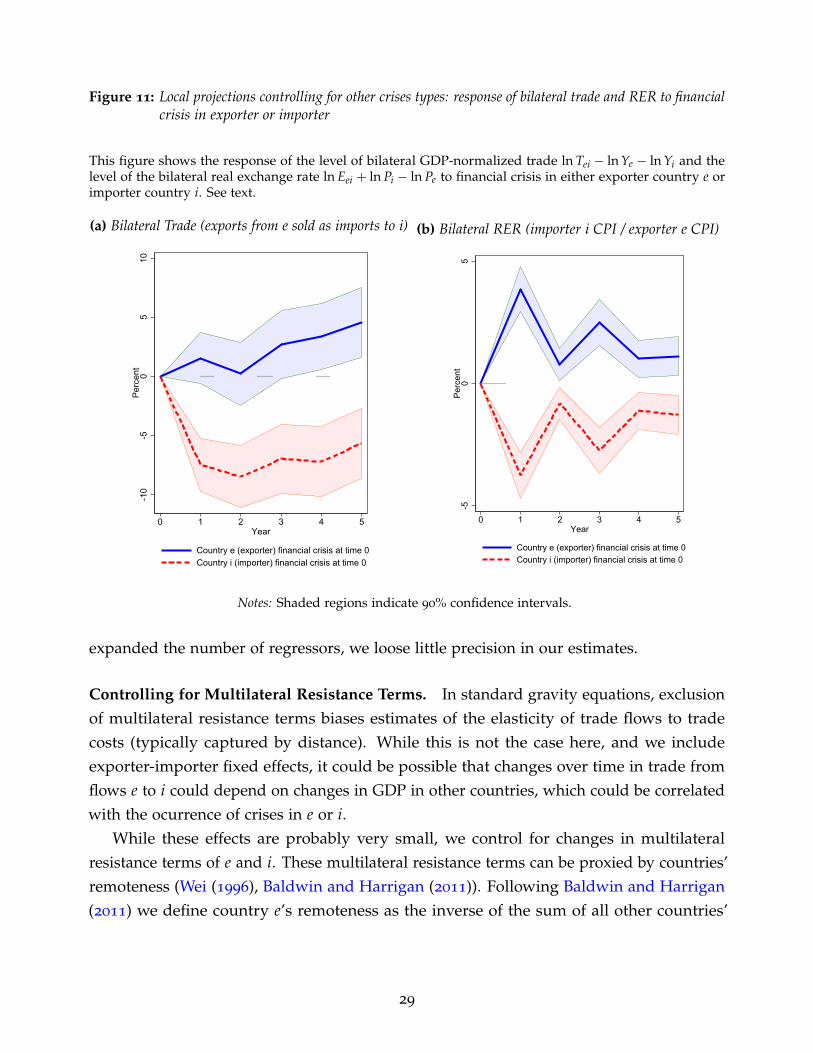
Figure 11: Local projections controlling for other crises types: response of bilateral trade and RER to financialcrisis in exporter or importer
This figure shows the response of the level of bilateral GDP-normalized trade ln Tei − ln Ye − ln Yi and thelevel of the bilateral real exchange rate ln Eei + ln Pi − ln Pe to financial crisis in either exporter country e orimporter country i. See text.
(a) Bilateral Trade (exports from e sold as imports to i)
-10
-50
510
Per
cent
0 1 2 3 4 5Year
Country e (exporter) financial crisis at time 0Country i (importer) financial crisis at time 0
(b) Bilateral RER (importer i CPI / exporter e CPI)
-50
5P
erce
nt
0 1 2 3 4 5Year
Country e (exporter) financial crisis at time 0Country i (importer) financial crisis at time 0
Notes: Shaded regions indicate 90% confidence intervals.
expanded the number of regressors, we loose little precision in our estimates.
Controlling for Multilateral Resistance Terms. In standard gravity equations, exclusionof multilateral resistance terms biases estimates of the elasticity of trade flows to tradecosts (typically captured by distance). While this is not the case here, and we includeexporter-importer fixed effects, it could be possible that changes over time in trade fromflows e to i could depend on changes in GDP in other countries, which could be correlatedwith the ocurrence of crises in e or i.
While these effects are probably very small, we control for changes in multilateralresistance terms of e and i. These multilateral resistance terms can be proxied by countries’remoteness (Wei (1996), Baldwin and Harrigan (2011)). Following Baldwin and Harrigan(2011) we define country e’s remoteness as the inverse of the sum of all other countries’
29
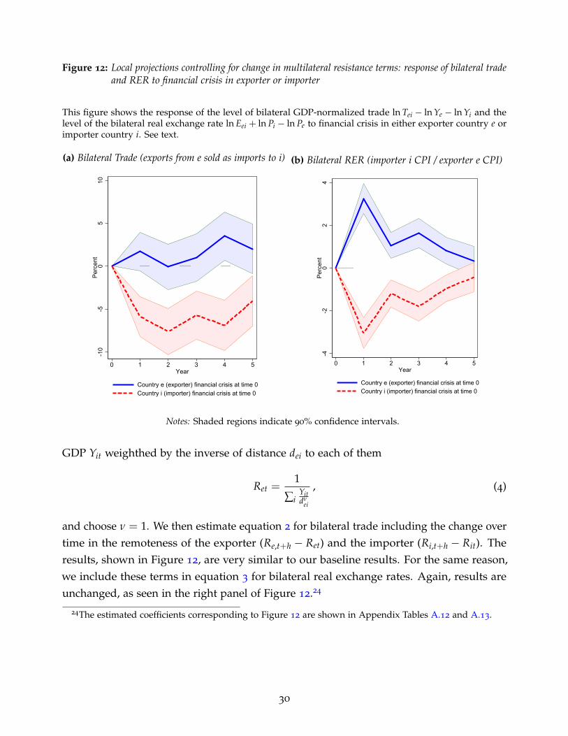
Figure 12: Local projections controlling for change in multilateral resistance terms: response of bilateral tradeand RER to financial crisis in exporter or importer
This figure shows the response of the level of bilateral GDP-normalized trade ln Tei − ln Ye − ln Yi and thelevel of the bilateral real exchange rate ln Eei + ln Pi − ln Pe to financial crisis in either exporter country e orimporter country i. See text.
(a) Bilateral Trade (exports from e sold as imports to i)
-10
-50
510
Per
cent
0 1 2 3 4 5Year
Country e (exporter) financial crisis at time 0Country i (importer) financial crisis at time 0
(b) Bilateral RER (importer i CPI / exporter e CPI)
-4-2
02
4P
erce
nt
0 1 2 3 4 5Year
Country e (exporter) financial crisis at time 0Country i (importer) financial crisis at time 0
Notes: Shaded regions indicate 90% confidence intervals.
GDP Yit weighthed by the inverse of distance dei to each of them
Ret =1
∑iYitdν
ei
, (4)
and choose ν = 1. We then estimate equation 2 for bilateral trade including the change overtime in the remoteness of the exporter (Re,t+h − Ret) and the importer (Ri,t+h − Rit). Theresults, shown in Figure 12, are very similar to our baseline results. For the same reason,we include these terms in equation 3 for bilateral real exchange rates. Again, results areunchanged, as seen in the right panel of Figure 12.24
24The estimated coefficients corresponding to Figure 12 are shown in Appendix Tables A.12 and A.13.
30
6. Crisis Endogeneity and Inverse Probability Weighting
We address the concern that financial crisis episodes might be endogenous using the methodof inverse probability weighting. This procedure assigns less weight in our bilateral tradeand RER regressions to observations that more likely to occur based on prior macroeconomicconditions. This correction for selection bias has been discussed in a time series context byAngrist, Jorda, and Kuersteiner (2018) and applied to the study of financial crises (Jorda,Schularick, and Taylor, 2011, 2016) and to the study of fiscal policy (Jorda and Taylor, 2016).
To start, we construct a first-stage estimator of the probability that country c has afinancial crisis at time t. As a predictor of crises, we use credit growth over the five-yearperiod leading to each crisis (between years t− 6 and t− 1). This choice follows Schularickand Taylor (2012) who show that credit growth is a powerful predictor of financial crises.25
We fit logit models for the probability of experiencing a financial crisis including eithercountry or country and year fixed effects. A successful predictor will maximize the rate oftrue positives and minimize the rate of false positives. A Receiver Operating Characteristic(ROC) curve reflects the trade-off between these two goals. The AUROC (Area underthe ROC curve) statistic summarizes the predictor’s quality in this regard.26 This statisticranges from 0.5 (for a predictor not different than a random guess) to 1 (for a perfectpredictor), and is independent of the cutoff value used to predict an outcome.
We report the first-stage results in Table 4. Column 1 corresponds to the benchmark casewith only country fixed effects, against which we assess the usefulness of credit growth asa crisis predictor. In column 2 we add credit growth, and in column 3 we add year fixedeffects.
As shown by Schularick and Taylor (2012), positive credit growth has a statisticallysignificant impact on the probability of experiencing a financial crisis. Further, the AUCstatistic in columns 2 and 3 is higher—and statistically different—than in our benchmarkcase in column 1, showing the contribution for credit growth as a financial crisis predictor.
Let us denote by pct the predicted probability that country c experiences a crisis at timet, and 1− pct the probability it does not. We construct weights for our bilateral trade andRER regressions based on these predicted probabilities as follows. We weight observationsin which both the exporter e and the importer i experience a financial crisis by 1
pet· pit. In
cases where both exporter and importer do not face a crisis, we assign weights 1(1− pet)·(1− pit)
.
Finally, we assign weights 1pet·(1− pit)
for cases with a crisis in the exporter only, and 1(1− pet)· pit
for cases with a crisis in the importer only.
25Credit is measured as domestic credit to GDP from the World Bank’s WDI dataset. Credit data is onlyavailable for our wide sample of developed and developing countries for the post-WW2 period.
26See Jorda and Taylor (2011) for a detailed explanation of these concepts.
31
We then re-estimate our bilateral trade regression using these weights. As shown inTable 5, the results are largely unchanged and our main message still holds. For example,we find (in panel (b)) a similar decrease by −5.1% in the normalized trade flow when thefinancial crisis event takes place in the importer country, while we had found a −6.1%change in the initial, unweighted results. As before, this impact is highly persistent.
Finally, we also repeat the estimation of the bilateral RER equation using IPW in table 6,also finding results similar to the baseline ones. The weighted results in panel (b) of table 6
show a +2.6% change when the financial crisis event takes place in the exporter country anda −2.5% change when it hits the importer country, where these impacts are very similar tothe baseline unweighted results of table 3 (a +3.3% change on impact following crises inthe exporter and a −3.1% change on impact following crises in the importer).
32
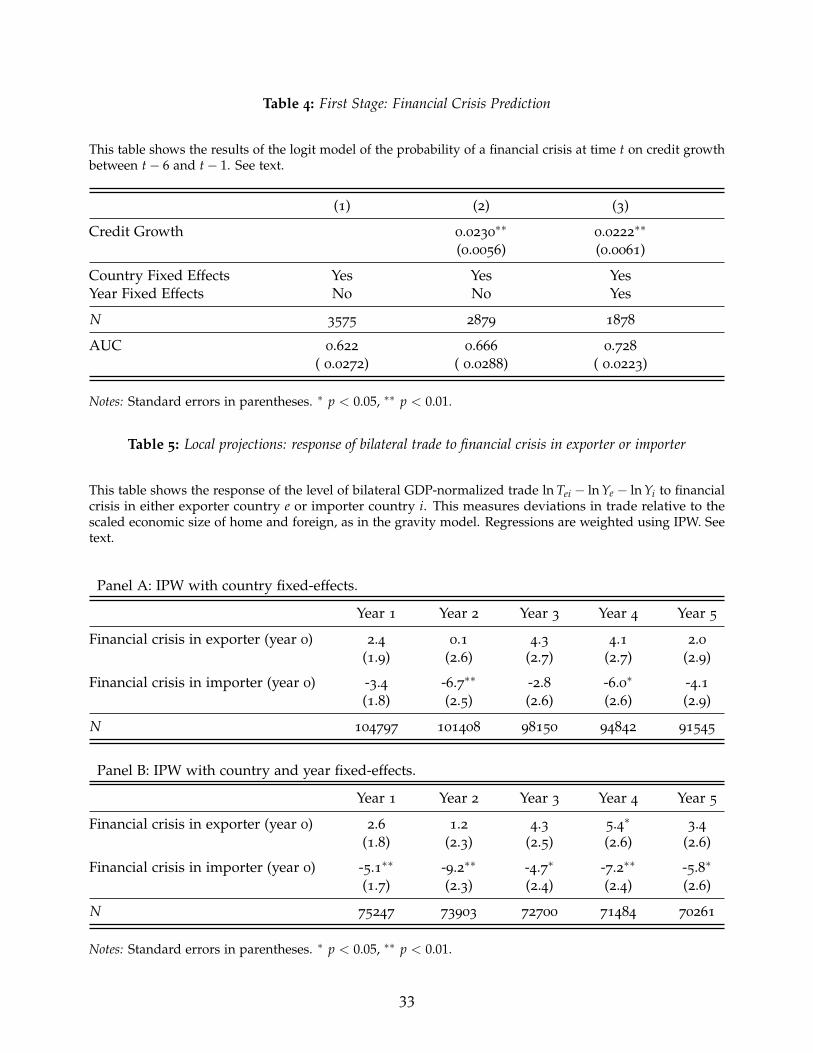
Table 4: First Stage: Financial Crisis Prediction
This table shows the results of the logit model of the probability of a financial crisis at time t on credit growthbetween t− 6 and t− 1. See text.
(1) (2) (3)
Credit Growth 0.0230∗∗
0.0222∗∗
(0.0056) (0.0061)
Country Fixed Effects Yes Yes YesYear Fixed Effects No No Yes
N 3575 2879 1878
AUC 0.622 0.666 0.728
( 0.0272) ( 0.0288) ( 0.0223)
Notes: Standard errors in parentheses. ∗ p < 0.05, ∗∗ p < 0.01.
Table 5: Local projections: response of bilateral trade to financial crisis in exporter or importer
This table shows the response of the level of bilateral GDP-normalized trade ln Tei − ln Ye − ln Yi to financialcrisis in either exporter country e or importer country i. This measures deviations in trade relative to thescaled economic size of home and foreign, as in the gravity model. Regressions are weighted using IPW. Seetext.
Panel A: IPW with country fixed-effects.
Year 1 Year 2 Year 3 Year 4 Year 5
Financial crisis in exporter (year 0) 2.4 0.1 4.3 4.1 2.0(1.9) (2.6) (2.7) (2.7) (2.9)
Financial crisis in importer (year 0) -3.4 -6.7∗∗ -2.8 -6.0∗ -4.1(1.8) (2.5) (2.6) (2.6) (2.9)
N 104797 101408 98150 94842 91545
Panel B: IPW with country and year fixed-effects.
Year 1 Year 2 Year 3 Year 4 Year 5
Financial crisis in exporter (year 0) 2.6 1.2 4.3 5.4∗ 3.4(1.8) (2.3) (2.5) (2.6) (2.6)
Financial crisis in importer (year 0) -5.1∗∗ -9.2∗∗ -4.7∗ -7.2∗∗ -5.8∗
(1.7) (2.3) (2.4) (2.4) (2.6)
N 75247 73903 72700 71484 70261
Notes: Standard errors in parentheses. ∗ p < 0.05, ∗∗ p < 0.01.
33
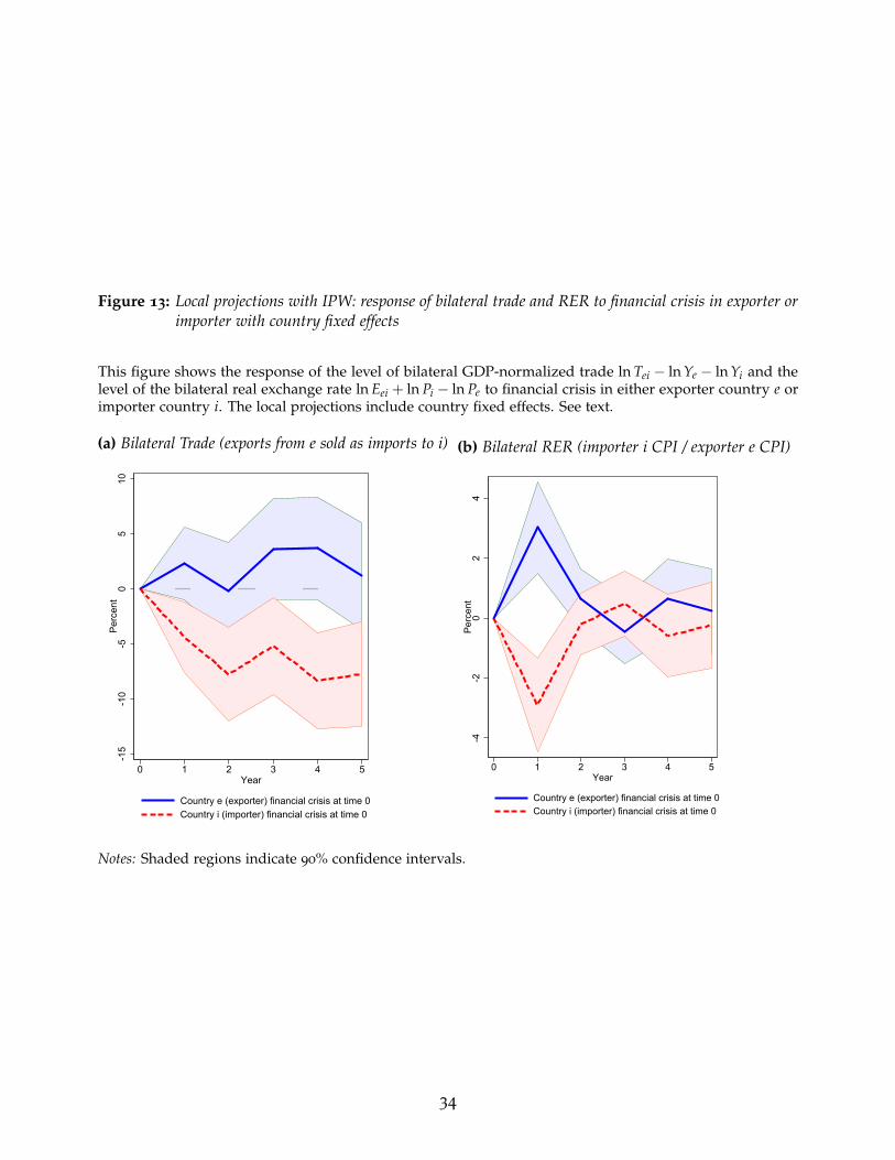
Figure 13: Local projections with IPW: response of bilateral trade and RER to financial crisis in exporter orimporter with country fixed effects
This figure shows the response of the level of bilateral GDP-normalized trade ln Tei − ln Ye − ln Yi and thelevel of the bilateral real exchange rate ln Eei + ln Pi − ln Pe to financial crisis in either exporter country e orimporter country i. The local projections include country fixed effects. See text.
(a) Bilateral Trade (exports from e sold as imports to i)
-15
-10
-50
510
Per
cent
0 1 2 3 4 5Year
Country e (exporter) financial crisis at time 0Country i (importer) financial crisis at time 0
(b) Bilateral RER (importer i CPI / exporter e CPI)
-4-2
02
4P
erce
nt
0 1 2 3 4 5Year
Country e (exporter) financial crisis at time 0Country i (importer) financial crisis at time 0
Notes: Shaded regions indicate 90% confidence intervals.
34
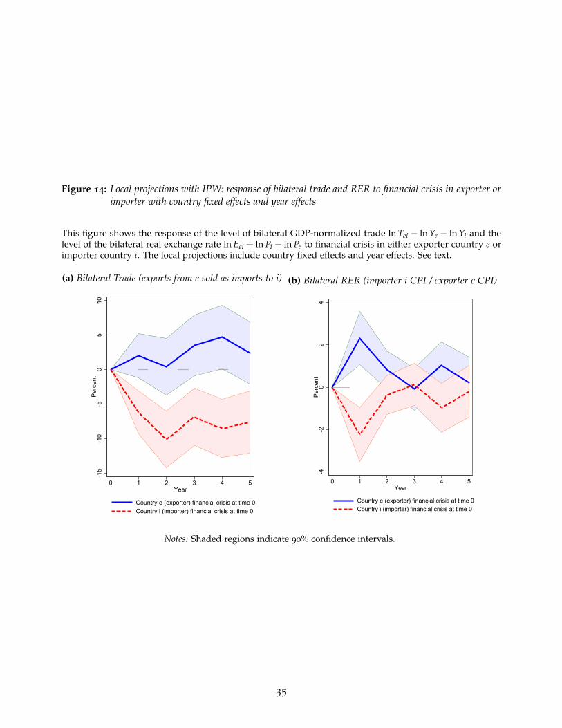
Figure 14: Local projections with IPW: response of bilateral trade and RER to financial crisis in exporter orimporter with country fixed effects and year effects
This figure shows the response of the level of bilateral GDP-normalized trade ln Tei − ln Ye − ln Yi and thelevel of the bilateral real exchange rate ln Eei + ln Pi − ln Pe to financial crisis in either exporter country e orimporter country i. The local projections include country fixed effects and year effects. See text.
(a) Bilateral Trade (exports from e sold as imports to i)
-15
-10
-50
510
Per
cent
0 1 2 3 4 5Year
Country e (exporter) financial crisis at time 0Country i (importer) financial crisis at time 0
(b) Bilateral RER (importer i CPI / exporter e CPI)
-4-2
02
4P
erce
nt
0 1 2 3 4 5Year
Country e (exporter) financial crisis at time 0Country i (importer) financial crisis at time 0
Notes: Shaded regions indicate 90% confidence intervals.
35
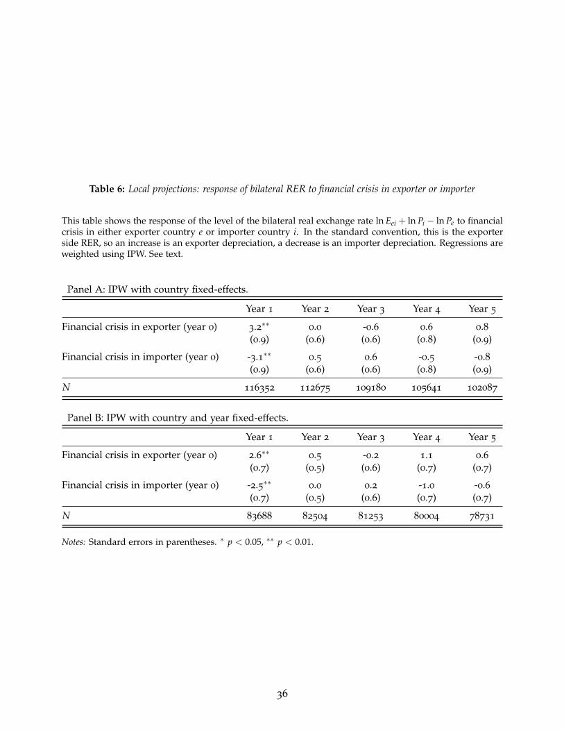
Table 6: Local projections: response of bilateral RER to financial crisis in exporter or importer
This table shows the response of the level of the bilateral real exchange rate ln Eei + ln Pi − ln Pe to financialcrisis in either exporter country e or importer country i. In the standard convention, this is the exporterside RER, so an increase is an exporter depreciation, a decrease is an importer depreciation. Regressions areweighted using IPW. See text.
Panel A: IPW with country fixed-effects.
Year 1 Year 2 Year 3 Year 4 Year 5
Financial crisis in exporter (year 0) 3.2∗∗ 0.0 -0.6 0.6 0.8(0.9) (0.6) (0.6) (0.8) (0.9)
Financial crisis in importer (year 0) -3.1∗∗ 0.5 0.6 -0.5 -0.8(0.9) (0.6) (0.6) (0.8) (0.9)
N 116352 112675 109180 105641 102087
Panel B: IPW with country and year fixed-effects.
Year 1 Year 2 Year 3 Year 4 Year 5
Financial crisis in exporter (year 0) 2.6∗∗ 0.5 -0.2 1.1 0.6(0.7) (0.5) (0.6) (0.7) (0.7)
Financial crisis in importer (year 0) -2.5∗∗ 0.0 0.2 -1.0 -0.6(0.7) (0.5) (0.6) (0.7) (0.7)
N 83688 82504 81253 80004 78731
Notes: Standard errors in parentheses. ∗ p < 0.05, ∗∗ p < 0.01.
36
7. Conclusions
We have developed a simple small open economy model, where a country is subject to“financial crisis” deleveraging shocks that impose tighter borrowing limits on householdsand/or firms. These shocks leave distinct statistical signatures in the empirical time seriesrecord, and they divide sharply between each type of shock.
Household deleveraging shocks are mainly demand shocks, contract imports, leaveexports largely unchanged, and depreciate the real exchange rate. Firm deleveragingshocks are mainly supply shocks, contract exports, leave imports largely unchanged, andappreciate the real exchange rate. We conjecture that these patterns will hold in a varietyof models with households and/or firms subject to financial frictions of this kind, so thelesson is more general.
Taking this model to the data, we compiled a crossed dataset of 200+ years of trade dataand dates of almost 200 financial crises in a large sample of countries. We use empiricalmethods to get a clearer picture of how financial distress affects trade and relative prices.Very clearly in the data, we see after a financial crisis event, on impact, that importscontract, exports hold steady or even rise, and the real exchange rate depreciate, with effectspersisting for five years. The effects are statistically significant: this pattern is the rule, notthe exception.
Based on both price and quantity evidence from the very long run, a robust interpretationemerges. History shows that on average financial crises are not, for the most part, a supplyshock. Rather, they are very clearly a negative shock to demand.
37
8. References
Abiad, Abdul, Prachi Mishra, and Petia Topalova. 2014. How Does Trade Evolve in theAftermath of Financial Crises? IMF Economic Review 62(2): 213–247.
Alessandria, George, Joseph P Kaboski, and Virgiliu Midrigan. 2010. The Great TradeCollapse of 2008–09: An Inventory Adjustment? IMF Economic Review 58(2): 254–294.
Amiti, Mary, and David E Weinstein. 2011. Exports and Financial Shocks. The QuarterlyJournal of Economics 126(4): 1841–1877.
Angrist, Joshua D, Oscar Jorda, and Guido M Kuersteiner. 2018. Semiparametric Estimatesof Monetary Policy Effects: String Theory Revisited. Journal of Business and EconomicStatistics 36(3): 371–387.
Baldwin, Richard, and James Harrigan. 2011. Zeros, Quality, and Space: Trade Theory andTrade Evidence. American Economic Journal: Microeconomics 3(2): 60–88.
Baldwin, Richard E, editor. 2009. The Great Trade Collapse: Causes, Consequences and Prospects.Centre for Economic Policy Research.
Barro, Robert J, and Jose F Ursua. 2008. Macroeconomic Crises Since 1870. Brookings Paperson Economic Activity 39(1 (Spring)): 255–350.
Behrens, Kristian, Gregory Corcos, and Giordano Mion. 2013. Trade Crisis? What TradeCrisis? The Review of Economics and Statistics 95(2): 702–709.
Bems, Rudolfs, Robert C Johnson, and Kei-Mu Yi. 2011. Vertical Linkages and the Collapseof Global Trade. The American Economic Review 101(3): 308–317.
Benigno, Pierpaolo, and Federica Romei. 2014. Debt Deleveraging and the Exchange Rate.Journal of International Economics 93(1): 1–16.
Bussiere, Matthieu, Giovanni Callegari, Fabio Ghironi, Giulia Sestieri, and Norihiko Yamano.2013. Estimating Trade Elasticities: Demand Composition and the Trade Collapse of2008-2009. American Economic Journal: Macroeconomics 5(3): 118–51.
Chor, Davin, and Kalina Manova. 2012. Off the Cliff and Back? Credit Conditions andInternational Trade during the Global Financial Crisis. Journal of International Economics87(1): 117–133.
Eaton, Jonathan, Samuel Kortum, Brent Neiman, and John Romalis. 2016. Trade and theGlobal Recession. The American Economic Review 106(11): 3401–38.
Eggertsson, Gauti B, and Paul Krugman. 2012. Debt, Deleveraging, and the Liquidity Trap:A Fisher-Minsky-Koo Approach. The Quarterly Journal of Economics 127(3): 1469–1513.
38
Fouquin, Michel, and Jules Hugot. 2016. Two Centuries of Bilateral Trade and Gravity Data:1827-2014. Working Paper .
Freund, Caroline L. 2009. The Trade Response to Global Downturns: Historical Evidence.World Bank Policy Research Working Paper Series 5015 .
Glick, Reuven, and Alan M Taylor. 2010. Collateral Damage: Trade Disruption and theEconomic Impact of War. The Review of Economics and Statistics 92(1): 102–127.
Hummels, David, Jun Ishii, and Kei-Mu Yi. 2001. The Nature and Growth of VerticalSpecialization in World Trade. Journal of International Economics 54(1): 75–96.
Iacovone, Leonardo, and Veronika Zavacka. 2009. Banking Crises and Exports: Lessonsfrom the Past. In The Great Trade Collapse: Causes, Consequences and Prospects, edited byBaldwin, Richard E. Centre for Economic Policy Research.
Jorda, Oscar. 2005. Estimation and Inference of Impulse Responses by Local Projections.The American Economic Review 95(1): 161–182.
Jorda, Oscar, Moritz Schularick, and Alan Taylor. 2013. When Credit Bites Back. Journal ofMoney, Credit and Banking 45(s2): 3–28.
Jorda, Oscar, Moritz Schularick, and Alan M Taylor. 2011. Financial Crises, Credit Booms,and External Imbalances: 140 Years of Lessons. IMF Economic Review 59(2): 340–378.
Jorda, Oscar, Moritz Schularick, and Alan M Taylor. 2016. Sovereigns versus Banks: Credit,Crises, and Consequences. Journal of the European Economic Association 14(1): 45–79.
Jorda, Oscar, and Alan M Taylor. 2011. Performance Evaluation of Zero Net-InvestmentStrategies. NBER Working Paper 17150 .
Jorda, Oscar, and Alan M Taylor. 2016. The Time for Austerity: Estimating the AverageTreatment Effect of Fiscal Policy. The Economic Journal 126(590): 219–255.
Levchenko, Andrei A, Logan T Lewis, and Linda L Tesar. 2010. The Collapse of InternationalTrade During the 2008–09 Crisis: In Search of the Smoking Gun. IMF Economic review58(2): 214–253.
Maddison, Angus. 1995. Monitoring the World Economy, 1820-1992 .
Maddison, Angus. 2001. The World Economy: A Millenial Perspective, Development Centreof the Organization for Economic Cooperation and Development.
Martin, Philippe, and Thomas Philippon. 2017. Inspecting the Mechanism: Leverage andthe Great Recession in the Eurozone. The American Economic Review 107(7): 1904–37.
Martinez, Joseba, and Thomas Philippon. 2014. Does a Currency Union Need a CapitalMarket Union? Working Paper .
Mian, Atif, Kamalesh Rao, and Amir Sufi. 2013. Household Balance Sheets, Consumption,and the Economic Slump. The Quarterly Journal of Economics 128(4): 1687–1726.
39
Mian, Atif, and Amir Sufi. 2014. What Explains the 2007–2009 Drop in Employment?Econometrica 82(6): 2197–2223.
Mian, Atif, Amir Sufi, and Emil Verner. 2017. Household Debt and Business CyclesWorldwide. The Quarterly Journal of Economics 132(4): 1755–1817.
Mitchell, B. 1992. International Historical Statistics Europe (1750-1988).
Mitchell, B. 1993. International History Statistics: the Americas (1750-1988).
Mitchell, B. 1995. International Historical Statistics Africa Asia and Oceania (1750-1988).
Monacelli, Tommaso. 2009. New Keynesian Models, Durable Goods, and Collateral Con-straints. Journal of Monetary Economics 56(2): 242–254.
Novy, Dennis, and Alan M Taylor. 2014. Trade and Uncertainty. Working Paper .
Reinhart, Carmen M. 2010. This Time is Different Chartbook: Country Histories on Debt,Default, and Financial Crises. NBER Working Paper 15815 .
Reinhart, Carmen M, and Kenneth S Rogoff. 2009. The Aftermath of Financial Crises. TheAmerican Economic Review 99(2): 466–72.
Reinhart, Carmen M, and Kenneth S Rogoff. 2011. From Financial Crash to Debt Crisis. TheAmerican Economic Review 101(5): 1676–1706.
Schularick, Moritz, and Alan M Taylor. 2012. Credit Booms Gone Bust: Monetary Policy,Leverage Cycles, and Financial Crises, 1870–2008. The American Economic Review 102(2):1029–1061.
Wei, Shang-Jin. 1996. Intra-national versus International Trade: How Stubborn are Nationsin Global Integration? NBER Working Paper 5531 .
40
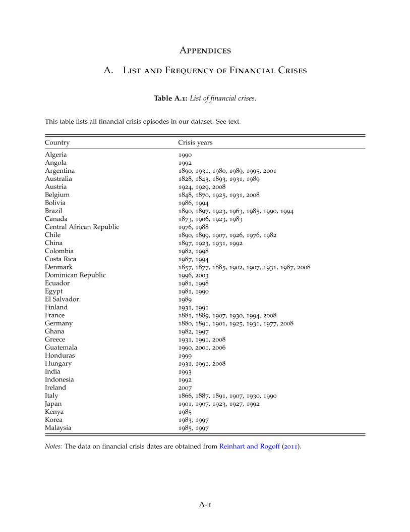
Appendices
A. List and Frequency of Financial Crises
Table A.1: List of financial crises.
This table lists all financial crisis episodes in our dataset. See text.
Country Crisis years
Algeria 1990
Angola 1992
Argentina 1890, 1931, 1980, 1989, 1995, 2001
Australia 1828, 1843, 1893, 1931, 1989
Austria 1924, 1929, 2008
Belgium 1848, 1870, 1925, 1931, 2008
Bolivia 1986, 1994
Brazil 1890, 1897, 1923, 1963, 1985, 1990, 1994
Canada 1873, 1906, 1923, 1983
Central African Republic 1976, 1988
Chile 1890, 1899, 1907, 1926, 1976, 1982
China 1897, 1923, 1931, 1992
Colombia 1982, 1998
Costa Rica 1987, 1994
Denmark 1857, 1877, 1885, 1902, 1907, 1931, 1987, 2008
Dominican Republic 1996, 2003
Ecuador 1981, 1998
Egypt 1981, 1990
El Salvador 1989
Finland 1931, 1991
France 1881, 1889, 1907, 1930, 1994, 2008
Germany 1880, 1891, 1901, 1925, 1931, 1977, 2008
Ghana 1982, 1997
Greece 1931, 1991, 2008
Guatemala 1990, 2001, 2006
Honduras 1999
Hungary 1931, 1991, 2008
India 1993
Indonesia 1992
Ireland 2007
Italy 1866, 1887, 1891, 1907, 1930, 1990
Japan 1901, 1907, 1923, 1927, 1992
Kenya 1985
Korea 1983, 1997
Malaysia 1985, 1997
Notes: The data on financial crisis dates are obtained from Reinhart and Rogoff (2011).
A-1
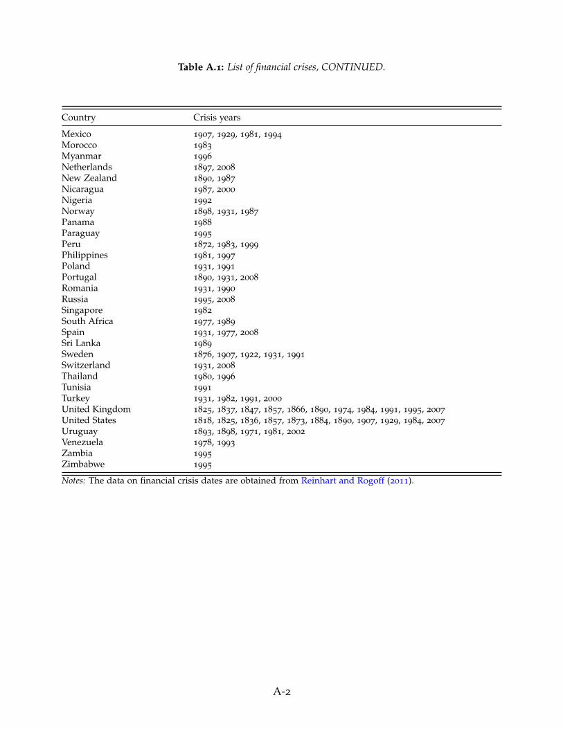
Table A.1: List of financial crises, CONTINUED.
Country Crisis years
Mexico 1907, 1929, 1981, 1994
Morocco 1983
Myanmar 1996
Netherlands 1897, 2008
New Zealand 1890, 1987
Nicaragua 1987, 2000
Nigeria 1992
Norway 1898, 1931, 1987
Panama 1988
Paraguay 1995
Peru 1872, 1983, 1999
Philippines 1981, 1997
Poland 1931, 1991
Portugal 1890, 1931, 2008
Romania 1931, 1990
Russia 1995, 2008
Singapore 1982
South Africa 1977, 1989
Spain 1931, 1977, 2008
Sri Lanka 1989
Sweden 1876, 1907, 1922, 1931, 1991
Switzerland 1931, 2008
Thailand 1980, 1996
Tunisia 1991
Turkey 1931, 1982, 1991, 2000
United Kingdom 1825, 1837, 1847, 1857, 1866, 1890, 1974, 1984, 1991, 1995, 2007
United States 1818, 1825, 1836, 1857, 1873, 1884, 1890, 1907, 1929, 1984, 2007
Uruguay 1893, 1898, 1971, 1981, 2002
Venezuela 1978, 1993
Zambia 1995
Zimbabwe 1995
Notes: The data on financial crisis dates are obtained from Reinhart and Rogoff (2011).
A-2
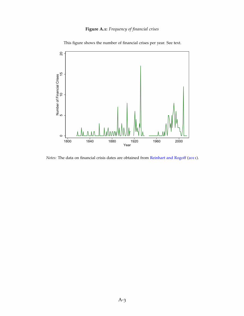
Figure A.1: Frequency of financial crises
This figure shows the number of financial crises per year. See text.
05
1015
20N
umbe
r of F
inan
cial
Cris
es
1800 1840 1880 1920 1960 2000Year
Notes: The data on financial crisis dates are obtained from Reinhart and Rogoff (2011).
A-3
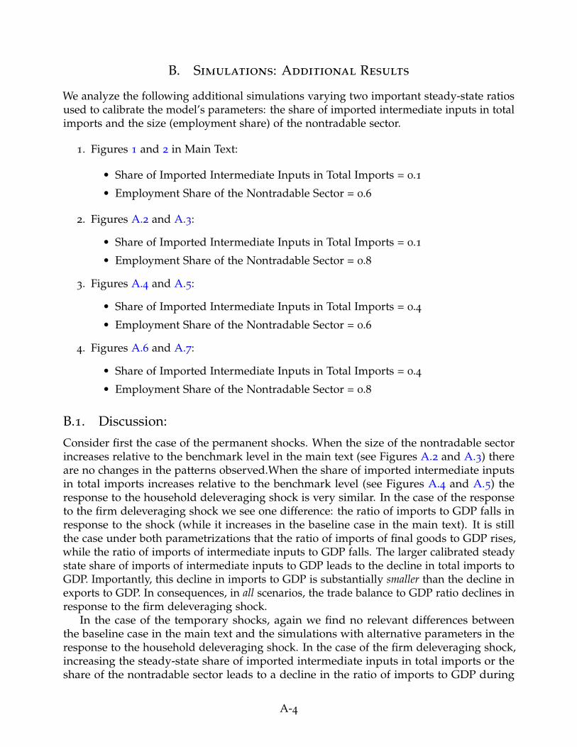
B. Simulations: Additional Results
We analyze the following additional simulations varying two important steady-state ratiosused to calibrate the model’s parameters: the share of imported intermediate inputs in totalimports and the size (employment share) of the nontradable sector.
1. Figures 1 and 2 in Main Text:
• Share of Imported Intermediate Inputs in Total Imports = 0.1
• Employment Share of the Nontradable Sector = 0.6
2. Figures A.2 and A.3:
• Share of Imported Intermediate Inputs in Total Imports = 0.1
• Employment Share of the Nontradable Sector = 0.8
3. Figures A.4 and A.5:
• Share of Imported Intermediate Inputs in Total Imports = 0.4
• Employment Share of the Nontradable Sector = 0.6
4. Figures A.6 and A.7:
• Share of Imported Intermediate Inputs in Total Imports = 0.4
• Employment Share of the Nontradable Sector = 0.8
B.1. Discussion:
Consider first the case of the permanent shocks. When the size of the nontradable sectorincreases relative to the benchmark level in the main text (see Figures A.2 and A.3) thereare no changes in the patterns observed.When the share of imported intermediate inputsin total imports increases relative to the benchmark level (see Figures A.4 and A.5) theresponse to the household deleveraging shock is very similar. In the case of the responseto the firm deleveraging shock we see one difference: the ratio of imports to GDP falls inresponse to the shock (while it increases in the baseline case in the main text). It is stillthe case under both parametrizations that the ratio of imports of final goods to GDP rises,while the ratio of imports of intermediate inputs to GDP falls. The larger calibrated steadystate share of imports of intermediate inputs to GDP leads to the decline in total imports toGDP. Importantly, this decline in imports to GDP is substantially smaller than the decline inexports to GDP. In consequences, in all scenarios, the trade balance to GDP ratio declines inresponse to the firm deleveraging shock.
In the case of the temporary shocks, again we find no relevant differences betweenthe baseline case in the main text and the simulations with alternative parameters in theresponse to the household deleveraging shock. In the case of the firm deleveraging shock,increasing the steady-state share of imported intermediate inputs in total imports or theshare of the nontradable sector leads to a decline in the ratio of imports to GDP during
A-4
the period when the borrowing limit falls. Once again, a key point is that in all cases thedecline in imports to GDP is smaller than the decline in exports to GDP and consequentlythe trade balance to GDP ratio declines in response to the firm deleveraging shock in allscenarios.
A-5
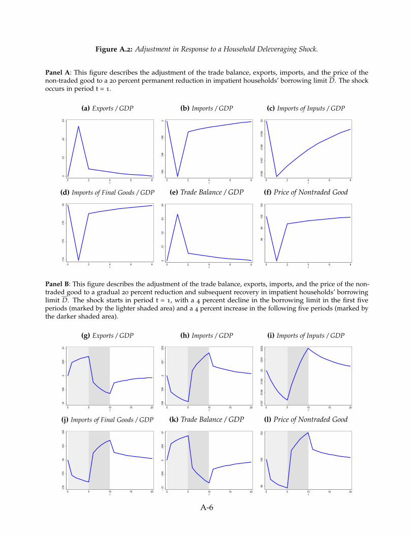
Figure A.2: Adjustment in Response to a Household Deleveraging Shock.
Panel A: This figure describes the adjustment of the trade balance, exports, imports, and the price of thenon-traded good to a 20 percent permanent reduction in impatient households’ borrowing limit D. The shockoccurs in period t = 1.
(a) Exports / GDP
.2.2
1.2
2.2
3
0 2 4 6 8t
(b) Imports / GDP
.194
.196
.198
.2
0 2 4 6 8t
(c) Imports of Inputs / GDP
.019
6.0
197
.019
8.0
199
.02
0 2 4 6 8t
(d) Imports of Final Goods / GDP
.174
.176
.178
.18
0 2 4 6 8t
(e) Trade Balance / GDP
0.0
1.0
2.0
3.0
4
0 2 4 6 8t
(f) Price of Nontraded Good
9698
100
102
0 2 4 6 8t
Panel B: This figure describes the adjustment of the trade balance, exports, imports, and the price of the non-traded good to a gradual 20 percent reduction and subsequent recovery in impatient households’ borrowinglimit D. The shock starts in period t = 1, with a 4 percent decline in the borrowing limit in the first fiveperiods (marked by the lighter shaded area) and a 4 percent increase in the following five periods (marked bythe darker shaded area).
(g) Exports / GDP
.19
.195
.2.2
05.2
1
0 5 10 15 20t
(h) Imports / GDP
.198
.199
.2.2
01.2
02
0 5 10 15 20t
(i) Imports of Inputs / GDP
.019
7.0
198
.019
9.0
2.0
201
.020
2
0 5 10 15 20t
(j) Imports of Final Goods / GDP
.178
.179
.18
.181
.182
0 5 10 15 20t
(k) Trade Balance / GDP
-.01
-.005
0.0
05.0
1
0 5 10 15 20t
(l) Price of Nontraded Good
9810
010
2
0 5 10 15 20t
A-6

Figure A.3: Adjustment in Response to a Firm Deleveraging Shock.
Panel A: This figure describes the adjustment of the trade balance, exports, imports, and the price of thenon-traded good to a 20 percent permanent reduction in firms’ borrowing limit δ. The shock occurs in periodt = 1.
(a) Exports / GDP
.17
.18
.19
.2.2
1.2
2
0 2 4 6 8t
(b) Imports / GDP
.19
.195
.2.2
05
0 2 4 6 8t
(c) Imports of Inputs / GDP
.014
.016
.018
.02
0 2 4 6 8t
(d) Imports of Final Goods / GDP
.175
.18
.185
.19
0 2 4 6 8t
(e) Trade Balance / GDP
-.04
-.02
0.0
2.0
4
0 2 4 6 8t
(f) Price of Nontraded Good
9011
013
00 2 4 6 8
t
Panel B: This figure describes the adjustment of the trade balance, exports, imports, and the price of thenon-traded good to a gradual 20 percent reduction and subsequent recovery in firms’ borrowing limit δ. Theshock starts in period t = 1, with a 4 percent decline in the borrowing limit in the first five periods (marked bythe lighter shaded area) and a 4 percent increase in the following five periods (marked by the darker shadedarea).
(g) Exports / GDP
.19
.2.2
1.2
2.2
3
0 5 10 15 20t
(h) Imports / GDP
.192
.194
.196
.198
.2
0 5 10 15 20t
(i) Imports of Inputs / GDP
.014
.016
.018
.02
0 5 10 15 20t
(j) Imports of Final Goods / GDP
.174
.176
.178
.18
.182
0 5 10 15 20t
(k) Trade Balance / GDP
-.01
0.0
1.0
2.0
3
0 5 10 15 20t
(l) Price of Nontraded Good
9010
011
012
0
0 5 10 15 20t
A-7
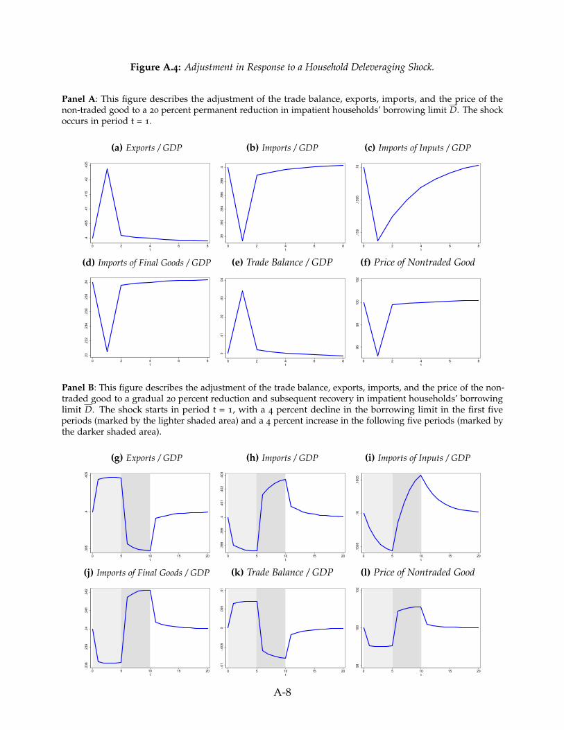
Figure A.4: Adjustment in Response to a Household Deleveraging Shock.
Panel A: This figure describes the adjustment of the trade balance, exports, imports, and the price of thenon-traded good to a 20 percent permanent reduction in impatient households’ borrowing limit D. The shockoccurs in period t = 1.
(a) Exports / GDP
.4.4
05.4
1.4
15.4
2.4
25
0 2 4 6 8t
(b) Imports / GDP
.39
.392
.394
.396
.398
.4
0 2 4 6 8t
(c) Imports of Inputs / GDP
.159
.159
5.1
6
0 2 4 6 8t
(d) Imports of Final Goods / GDP
.23
.232
.234
.236
.238
.24
0 2 4 6 8t
(e) Trade Balance / GDP
0.0
1.0
2.0
3.0
4
0 2 4 6 8t
(f) Price of Nontraded Good
9698
100
102
0 2 4 6 8t
Panel B: This figure describes the adjustment of the trade balance, exports, imports, and the price of the non-traded good to a gradual 20 percent reduction and subsequent recovery in impatient households’ borrowinglimit D. The shock starts in period t = 1, with a 4 percent decline in the borrowing limit in the first fiveperiods (marked by the lighter shaded area) and a 4 percent increase in the following five periods (marked bythe darker shaded area).
(g) Exports / GDP
.395
.4.4
05
0 5 10 15 20t
(h) Imports / GDP
.398
.399
.4.4
01.4
02.4
03
0 5 10 15 20t
(i) Imports of Inputs / GDP
.159
5.1
6.1
605
0 5 10 15 20t
(j) Imports of Final Goods / GDP
.238
.239
.24
.241
.242
0 5 10 15 20t
(k) Trade Balance / GDP
-.01
-.005
0.0
05.0
1
0 5 10 15 20t
(l) Price of Nontraded Good
9810
010
2
0 5 10 15 20t
A-8
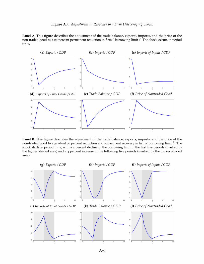
Figure A.5: Adjustment in Response to a Firm Deleveraging Shock.
Panel A: This figure describes the adjustment of the trade balance, exports, imports, and the price of thenon-traded good to a 20 percent permanent reduction in firms’ borrowing limit δ. The shock occurs in periodt = 1.
(a) Exports / GDP
.3.3
2.3
4.3
6.3
8.4
0 2 4 6 8t
(b) Imports / GDP
.36
.37
.38
.39
.4
0 2 4 6 8t
(c) Imports of Inputs / GDP
.1.1
2.1
4.1
6
0 2 4 6 8t
(d) Imports of Final Goods / GDP
.24
.25
.26
.27
.28
0 2 4 6 8t
(e) Trade Balance / GDP
-.08
-.06
-.04
-.02
0
0 2 4 6 8t
(f) Price of Nontraded Good
9011
013
00 2 4 6 8
t
Panel B: This figure describes the adjustment of the trade balance, exports, imports, and the price of thenon-traded good to a gradual 20 percent reduction and subsequent recovery in firms’ borrowing limit δ. Theshock starts in period t = 1, with a 4 percent decline in the borrowing limit in the first five periods (marked bythe lighter shaded area) and a 4 percent increase in the following five periods (marked by the darker shadedarea).
(g) Exports / GDP
.34
.36
.38
.4.4
2
0 5 10 15 20t
(h) Imports / GDP
.375
.38
.385
.39
.395
.4
0 5 10 15 20t
(i) Imports of Inputs / GDP
.11
.12
.13
.14
.15
.16
0 5 10 15 20t
(j) Imports of Final Goods / GDP
.23
.24
.25
.26
.27
0 5 10 15 20t
(k) Trade Balance / GDP
-.04
-.02
0.0
2.0
4
0 5 10 15 20t
(l) Price of Nontraded Good
9010
011
012
0
0 5 10 15 20t
A-9
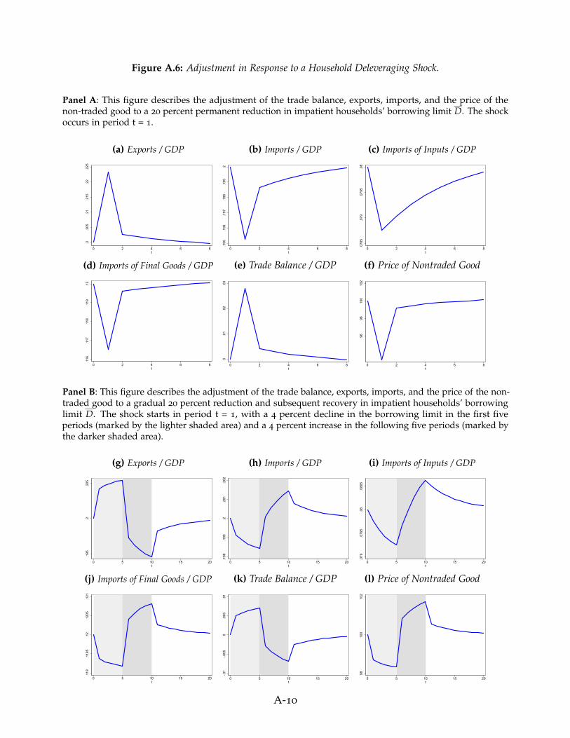
Figure A.6: Adjustment in Response to a Household Deleveraging Shock.
Panel A: This figure describes the adjustment of the trade balance, exports, imports, and the price of thenon-traded good to a 20 percent permanent reduction in impatient households’ borrowing limit D. The shockoccurs in period t = 1.
(a) Exports / GDP
.2.2
05.2
1.2
15.2
2.2
25
0 2 4 6 8t
(b) Imports / GDP
.195
.196
.197
.198
.199
.2
0 2 4 6 8t
(c) Imports of Inputs / GDP
.078
5.0
79.0
795
.08
0 2 4 6 8t
(d) Imports of Final Goods / GDP
.116
.117
.118
.119
.12
0 2 4 6 8t
(e) Trade Balance / GDP
0.0
1.0
2.0
3
0 2 4 6 8t
(f) Price of Nontraded Good
9698
100
102
0 2 4 6 8t
Panel B: This figure describes the adjustment of the trade balance, exports, imports, and the price of the non-traded good to a gradual 20 percent reduction and subsequent recovery in impatient households’ borrowinglimit D. The shock starts in period t = 1, with a 4 percent decline in the borrowing limit in the first fiveperiods (marked by the lighter shaded area) and a 4 percent increase in the following five periods (marked bythe darker shaded area).
(g) Exports / GDP
.195
.2.2
05
0 5 10 15 20t
(h) Imports / GDP
.198
.199
.2.2
01.2
02
0 5 10 15 20t
(i) Imports of Inputs / GDP
.079
.079
5.0
8.0
805
0 5 10 15 20t
(j) Imports of Final Goods / GDP
.119
.119
5.1
2.1
205
.121
0 5 10 15 20t
(k) Trade Balance / GDP
-.01
-.005
0.0
05.0
1
0 5 10 15 20t
(l) Price of Nontraded Good
9810
010
2
0 5 10 15 20t
A-10
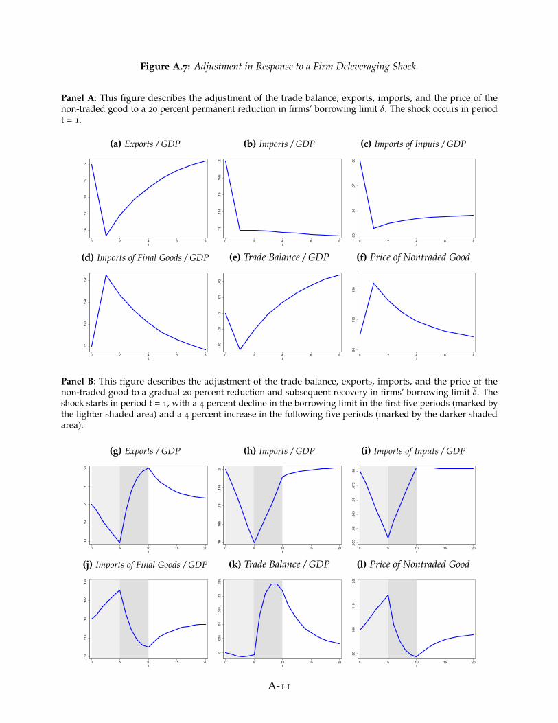
Figure A.7: Adjustment in Response to a Firm Deleveraging Shock.
Panel A: This figure describes the adjustment of the trade balance, exports, imports, and the price of thenon-traded good to a 20 percent permanent reduction in firms’ borrowing limit δ. The shock occurs in periodt = 1.
(a) Exports / GDP
.16
.17
.18
.19
.2
0 2 4 6 8t
(b) Imports / GDP
.18
.185
.19
.195
.2
0 2 4 6 8t
(c) Imports of Inputs / GDP
.05
.06
.07
.08
0 2 4 6 8t
(d) Imports of Final Goods / GDP
.12
.122
.124
.126
0 2 4 6 8t
(e) Trade Balance / GDP
-.02
-.01
0.0
1.0
2
0 2 4 6 8t
(f) Price of Nontraded Good
9011
013
00 2 4 6 8
t
Panel B: This figure describes the adjustment of the trade balance, exports, imports, and the price of thenon-traded good to a gradual 20 percent reduction and subsequent recovery in firms’ borrowing limit δ. Theshock starts in period t = 1, with a 4 percent decline in the borrowing limit in the first five periods (marked bythe lighter shaded area) and a 4 percent increase in the following five periods (marked by the darker shadedarea).
(g) Exports / GDP
.18
.19
.2.2
1.2
2
0 5 10 15 20t
(h) Imports / GDP
.18
.185
.19
.195
.2
0 5 10 15 20t
(i) Imports of Inputs / GDP
.055
.06
.065
.07
.075
.08
0 5 10 15 20t
(j) Imports of Final Goods / GDP
.116
.118
.12
.122
.124
0 5 10 15 20t
(k) Trade Balance / GDP
0.0
05.0
1.0
15.0
2.0
25
0 5 10 15 20t
(l) Price of Nontraded Good
9010
011
012
0
0 5 10 15 20t
A-11
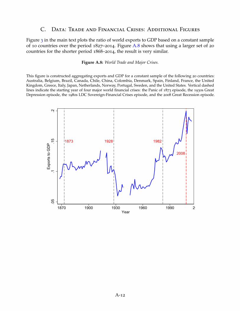
C. Data: Trade and Financial Crises: Additional Figures
Figure 3 in the main text plots the ratio of world exports to GDP based on a constant sampleof 10 countries over the period 1827–2014. Figure A.8 shows that using a larger set of 20
countries for the shorter period 1868–2014, the result is very similar.
Figure A.8: World Trade and Major Crises.
This figure is constructed aggregating exports and GDP for a constant sample of the following 20 countries:Australia, Belgium, Brazil, Canada, Chile, China, Colombia, Denmark, Spain, Finland, France, the UnitedKingdom, Greece, Italy, Japan, Netherlands, Norway, Portugal, Sweden, and the United States. Vertical dashedlines indicate the starting year of four major world financial crises: the Panic of 1873 episode, the 1930s GreatDepression episode, the 1980s LDC Sovereign-Financial Crises episode, and the 2008 Great Recession episode.
1873 1928 1982
2008
.05
.1.1
5.2
Exp
orts
to G
DP
1870 1900 1930 1960 1990 2020Year
A-12
D. Total Trade: Additional Tables
This section includes the tables with estimates corresponding to Figures 5 and 6 in Section4 in the main text.
• Table A.2 shows the results of the estimation of equation 1 splitting the sample intosubperiods. It corresponds to Figure 5 in the main text.
• Table A.3 shows the results of the estimation of equation 1 splitting the sample intogroups according to countries’ level of development. It corresponds to Figure 6 in themain text.
A-13
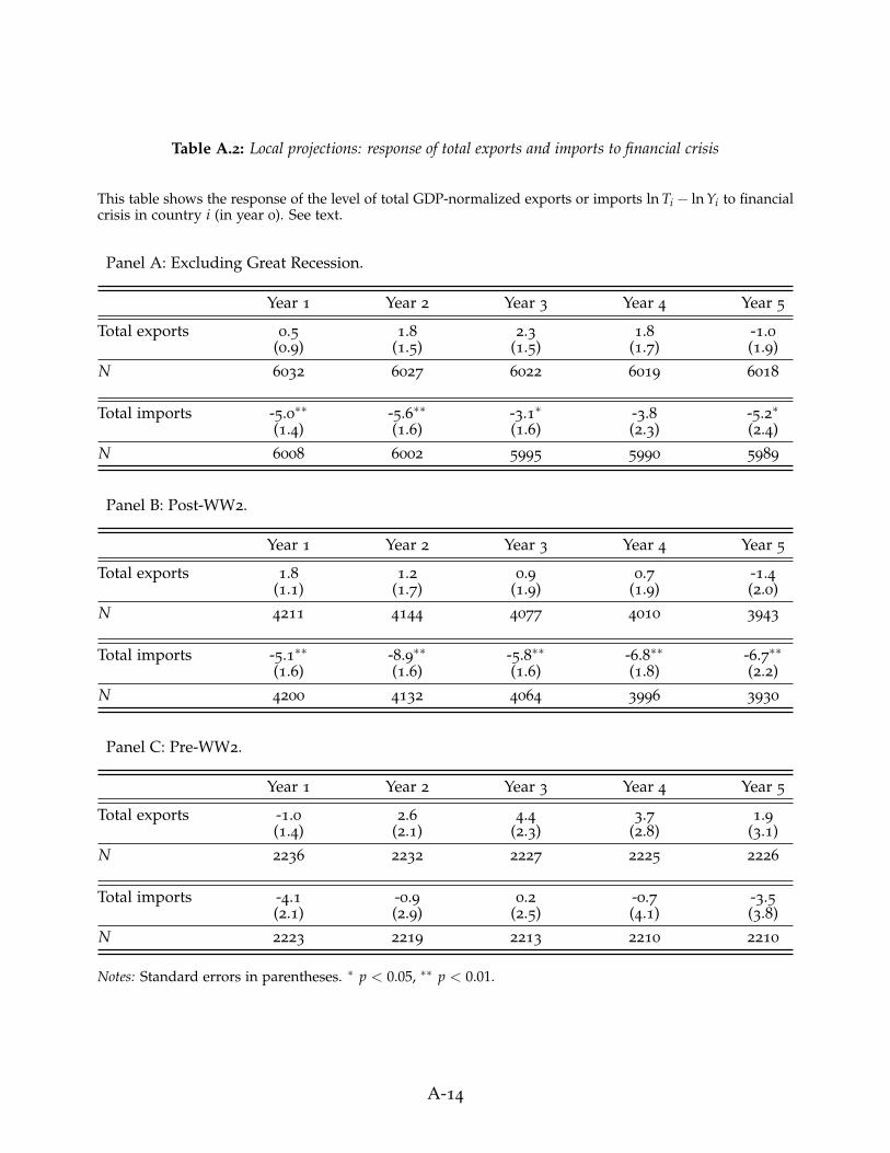
Table A.2: Local projections: response of total exports and imports to financial crisis
This table shows the response of the level of total GDP-normalized exports or imports ln Ti − ln Yi to financialcrisis in country i (in year 0). See text.
Panel A: Excluding Great Recession.
Year 1 Year 2 Year 3 Year 4 Year 5
Total exports 0.5 1.8 2.3 1.8 -1.0(0.9) (1.5) (1.5) (1.7) (1.9)
N 6032 6027 6022 6019 6018
Total imports -5.0∗∗ -5.6∗∗ -3.1∗ -3.8 -5.2∗(1.4) (1.6) (1.6) (2.3) (2.4)
N 6008 6002 5995 5990 5989
Panel B: Post-WW2.
Year 1 Year 2 Year 3 Year 4 Year 5
Total exports 1.8 1.2 0.9 0.7 -1.4(1.1) (1.7) (1.9) (1.9) (2.0)
N 4211 4144 4077 4010 3943
Total imports -5.1∗∗ -8.9∗∗ -5.8∗∗ -6.8∗∗ -6.7∗∗(1.6) (1.6) (1.6) (1.8) (2.2)
N 4200 4132 4064 3996 3930
Panel C: Pre-WW2.
Year 1 Year 2 Year 3 Year 4 Year 5
Total exports -1.0 2.6 4.4 3.7 1.9(1.4) (2.1) (2.3) (2.8) (3.1)
N 2236 2232 2227 2225 2226
Total imports -4.1 -0.9 0.2 -0.7 -3.5(2.1) (2.9) (2.5) (4.1) (3.8)
N 2223 2219 2213 2210 2210
Notes: Standard errors in parentheses. ∗ p < 0.05, ∗∗ p < 0.01.
A-14
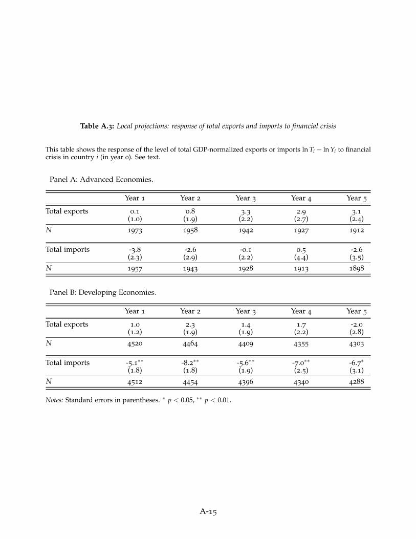
Table A.3: Local projections: response of total exports and imports to financial crisis
This table shows the response of the level of total GDP-normalized exports or imports ln Ti − ln Yi to financialcrisis in country i (in year 0). See text.
Panel A: Advanced Economies.
Year 1 Year 2 Year 3 Year 4 Year 5
Total exports 0.1 0.8 3.3 2.9 3.1(1.0) (1.9) (2.2) (2.7) (2.4)
N 1973 1958 1942 1927 1912
Total imports -3.8 -2.6 -0.1 0.5 -2.6(2.3) (2.9) (2.2) (4.4) (3.5)
N 1957 1943 1928 1913 1898
Panel B: Developing Economies.
Year 1 Year 2 Year 3 Year 4 Year 5
Total exports 1.0 2.3 1.4 1.7 -2.0(1.2) (1.9) (1.9) (2.2) (2.8)
N 4520 4464 4409 4355 4303
Total imports -5.1∗∗ -8.2∗∗ -5.6∗∗ -7.0∗∗ -6.7∗(1.8) (1.8) (1.9) (2.5) (3.1)
N 4512 4454 4396 4340 4288
Notes: Standard errors in parentheses. ∗ p < 0.05, ∗∗ p < 0.01.
A-15
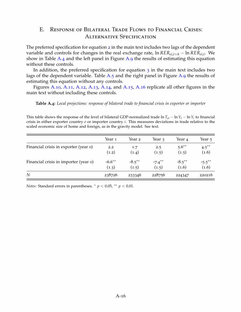
E. Response of Bilateral Trade Flows to Financial Crises:Alternative Specification
The preferred specification for equation 2 in the main text includes two lags of the dependentvariable and controls for changes in the real exchange rate, ln RERei,t+h − ln RERei,t. Weshow in Table A.4 and the left panel in Figure A.9 the results of estimating this equationwithout these controls.
In addition, the preferred specification for equation 3 in the main text includes twolags of the dependent variable. Table A.5 and the right panel in Figure A.9 the results ofestimating this equation without any controls.
Figures A.10, A.11, A.12, A.13, A.14, and A.15, A.16 replicate all other figures in themain text without including these controls.
Table A.4: Local projections: response of bilateral trade to financial crisis in exporter or importer
This table shows the response of the level of bilateral GDP-normalized trade ln Tei − ln Ye − ln Yi to financialcrisis in either exporter country e or importer country i. This measures deviations in trade relative to thescaled economic size of home and foreign, as in the gravity model. See text.
Year 1 Year 2 Year 3 Year 4 Year 5
Financial crisis in exporter (year 0) 2.2 1.7 2.5 5.6∗∗ 4.5∗∗
(1.2) (1.4) (1.5) (1.5) (1.6)
Financial crisis in importer (year 0) -6.6∗∗ -8.5∗∗ -7.4∗∗ -8.5∗∗ -5.5∗∗
(1.3) (1.5) (1.5) (1.6) (1.6)
N 238726 233346 228756 224347 220216
Notes: Standard errors in parentheses. ∗ p < 0.05, ∗∗ p < 0.01.
A-16
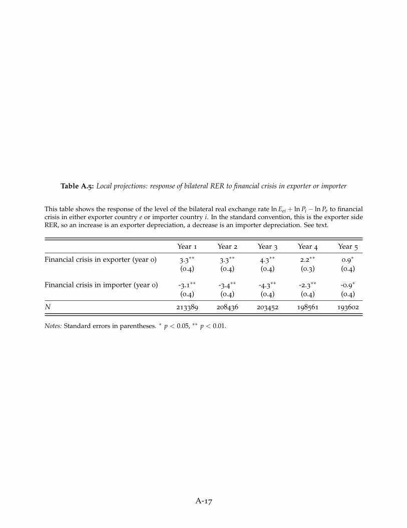
Table A.5: Local projections: response of bilateral RER to financial crisis in exporter or importer
This table shows the response of the level of the bilateral real exchange rate ln Eei + ln Pi − ln Pe to financialcrisis in either exporter country e or importer country i. In the standard convention, this is the exporter sideRER, so an increase is an exporter depreciation, a decrease is an importer depreciation. See text.
Year 1 Year 2 Year 3 Year 4 Year 5
Financial crisis in exporter (year 0) 3.3∗∗ 3.3∗∗ 4.3∗∗ 2.2∗∗ 0.9∗
(0.4) (0.4) (0.4) (0.3) (0.4)
Financial crisis in importer (year 0) -3.1∗∗ -3.4∗∗ -4.3∗∗ -2.3∗∗ -0.9∗
(0.4) (0.4) (0.4) (0.4) (0.4)
N 213389 208436 203452 198561 193602
Notes: Standard errors in parentheses. ∗ p < 0.05, ∗∗ p < 0.01.
A-17
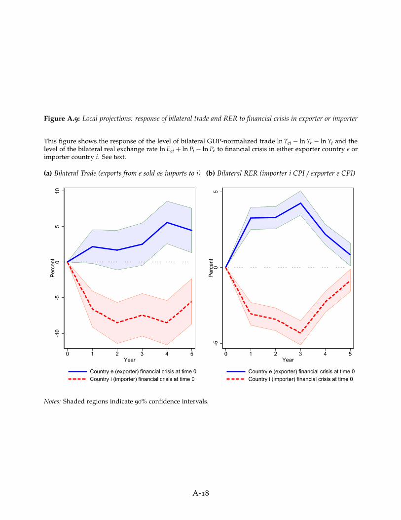
Figure A.9: Local projections: response of bilateral trade and RER to financial crisis in exporter or importer
This figure shows the response of the level of bilateral GDP-normalized trade ln Tei − ln Ye − ln Yi and thelevel of the bilateral real exchange rate ln Eei + ln Pi − ln Pe to financial crisis in either exporter country e orimporter country i. See text.
(a) Bilateral Trade (exports from e sold as imports to i)
-10
-50
510
Per
cent
0 1 2 3 4 5Year
Country e (exporter) financial crisis at time 0Country i (importer) financial crisis at time 0
(b) Bilateral RER (importer i CPI / exporter e CPI)
-50
5P
erce
nt
0 1 2 3 4 5Year
Country e (exporter) financial crisis at time 0Country i (importer) financial crisis at time 0
Notes: Shaded regions indicate 90% confidence intervals.
A-18
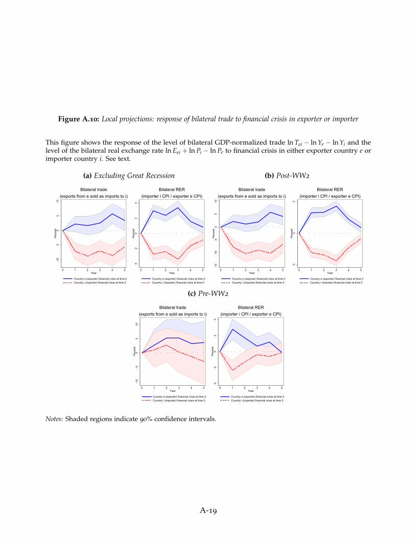
Figure A.10: Local projections: response of bilateral trade to financial crisis in exporter or importer
This figure shows the response of the level of bilateral GDP-normalized trade ln Tei − ln Ye − ln Yi and thelevel of the bilateral real exchange rate ln Eei + ln Pi − ln Pe to financial crisis in either exporter country e orimporter country i. See text.
(a) Excluding Great Recession
-10
-50
510
Per
cent
0 1 2 3 4 5Year
Country e (exporter) financial crisis at time 0Country i (importer) financial crisis at time 0
Bilateral trade(exports from e sold as imports to i)
-4-2
02
4P
erce
nt
0 1 2 3 4 5Year
Country e (exporter) financial crisis at time 0Country i (importer) financial crisis at time 0
Bilateral RER(importer i CPI / exporter e CPI)
(b) Post-WW2
-15
-10
-50
510
Per
cent
0 1 2 3 4 5Year
Country e (exporter) financial crisis at time 0Country i (importer) financial crisis at time 0
Bilateral trade(exports from e sold as imports to i)
-50
5P
erce
nt
0 1 2 3 4 5Year
Country e (exporter) financial crisis at time 0Country i (importer) financial crisis at time 0
Bilateral RER(importer i CPI / exporter e CPI)
(c) Pre-WW2
-10
-50
510
Per
cent
0 1 2 3 4 5Year
Country e (exporter) financial crisis at time 0Country i (importer) financial crisis at time 0
Bilateral trade(exports from e sold as imports to i)
-4-2
02
4P
erce
nt
0 1 2 3 4 5Year
Country e (exporter) financial crisis at time 0Country i (importer) financial crisis at time 0
Bilateral RER(importer i CPI / exporter e CPI)
Notes: Shaded regions indicate 90% confidence intervals.
A-19
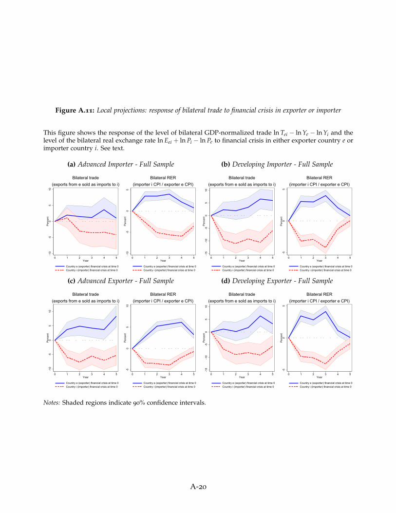
Figure A.11: Local projections: response of bilateral trade to financial crisis in exporter or importer
This figure shows the response of the level of bilateral GDP-normalized trade ln Tei − ln Ye − ln Yi and thelevel of the bilateral real exchange rate ln Eei + ln Pi − ln Pe to financial crisis in either exporter country e orimporter country i. See text.
(a) Advanced Importer - Full Sample
-10
-50
510
Per
cent
0 1 2 3 4 5Year
Country e (exporter) financial crisis at time 0Country i (importer) financial crisis at time 0
Bilateral trade(exports from e sold as imports to i)
-10
-50
5P
erce
nt
0 1 2 3 4 5Year
Country e (exporter) financial crisis at time 0Country i (importer) financial crisis at time 0
Bilateral RER(importer i CPI / exporter e CPI)
(b) Developing Importer - Full Sample
-15
-10
-50
510
Per
cent
0 1 2 3 4 5Year
Country e (exporter) financial crisis at time 0Country i (importer) financial crisis at time 0
Bilateral trade(exports from e sold as imports to i)
-50
5P
erce
nt
0 1 2 3 4 5Year
Country e (exporter) financial crisis at time 0Country i (importer) financial crisis at time 0
Bilateral RER(importer i CPI / exporter e CPI)
(c) Advanced Exporter - Full Sample
-10
-50
510
Per
cent
0 1 2 3 4 5Year
Country e (exporter) financial crisis at time 0Country i (importer) financial crisis at time 0
Bilateral trade(exports from e sold as imports to i)
-50
510
Per
cent
0 1 2 3 4 5Year
Country e (exporter) financial crisis at time 0Country i (importer) financial crisis at time 0
Bilateral RER(importer i CPI / exporter e CPI)
(d) Developing Exporter - Full Sample
-15
-10
-50
510
Per
cent
0 1 2 3 4 5Year
Country e (exporter) financial crisis at time 0Country i (importer) financial crisis at time 0
Bilateral trade(exports from e sold as imports to i)
-50
5P
erce
nt
0 1 2 3 4 5Year
Country e (exporter) financial crisis at time 0Country i (importer) financial crisis at time 0
Bilateral RER(importer i CPI / exporter e CPI)
Notes: Shaded regions indicate 90% confidence intervals.
A-20
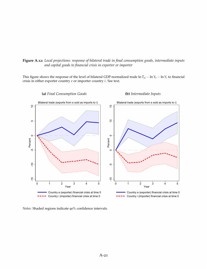
Figure A.12: Local projections: response of bilateral trade in final consumption goods, intermediate inputsand capital goods to financial crisis in exporter or importer
This figure shows the response of the level of bilateral GDP-normalized trade ln Tei − ln Ye − ln Yi to financialcrisis in either exporter country e or importer country i. See text.
(a) Final Consumption Goods
-15
-10
-50
510
Per
cent
0 1 2 3 4 5Year
Country e (exporter) financial crisis at time 0Country i (importer) financial crisis at time 0
Bilateral trade (exports from e sold as imports to i)
(b) Intermediate Inputs
-10
-50
510
15P
erce
nt
0 1 2 3 4 5Year
Country e (exporter) financial crisis at time 0Country i (importer) financial crisis at time 0
Bilateral trade (exports from e sold as imports to i)
Notes: Shaded regions indicate 90% confidence intervals.
A-21
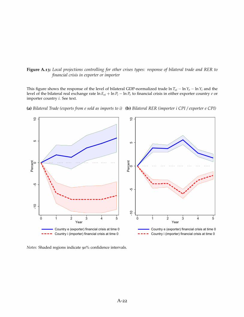
Figure A.13: Local projections controlling for other crises types: response of bilateral trade and RER tofinancial crisis in exporter or importer
This figure shows the response of the level of bilateral GDP-normalized trade ln Tei − ln Ye − ln Yi and thelevel of the bilateral real exchange rate ln Eei + ln Pi − ln Pe to financial crisis in either exporter country e orimporter country i. See text.
(a) Bilateral Trade (exports from e sold as imports to i)
-10
-50
510
Per
cent
0 1 2 3 4 5Year
Country e (exporter) financial crisis at time 0Country i (importer) financial crisis at time 0
(b) Bilateral RER (importer i CPI / exporter e CPI)
-10
-50
510
Per
cent
0 1 2 3 4 5Year
Country e (exporter) financial crisis at time 0Country i (importer) financial crisis at time 0
Notes: Shaded regions indicate 90% confidence intervals.
A-22
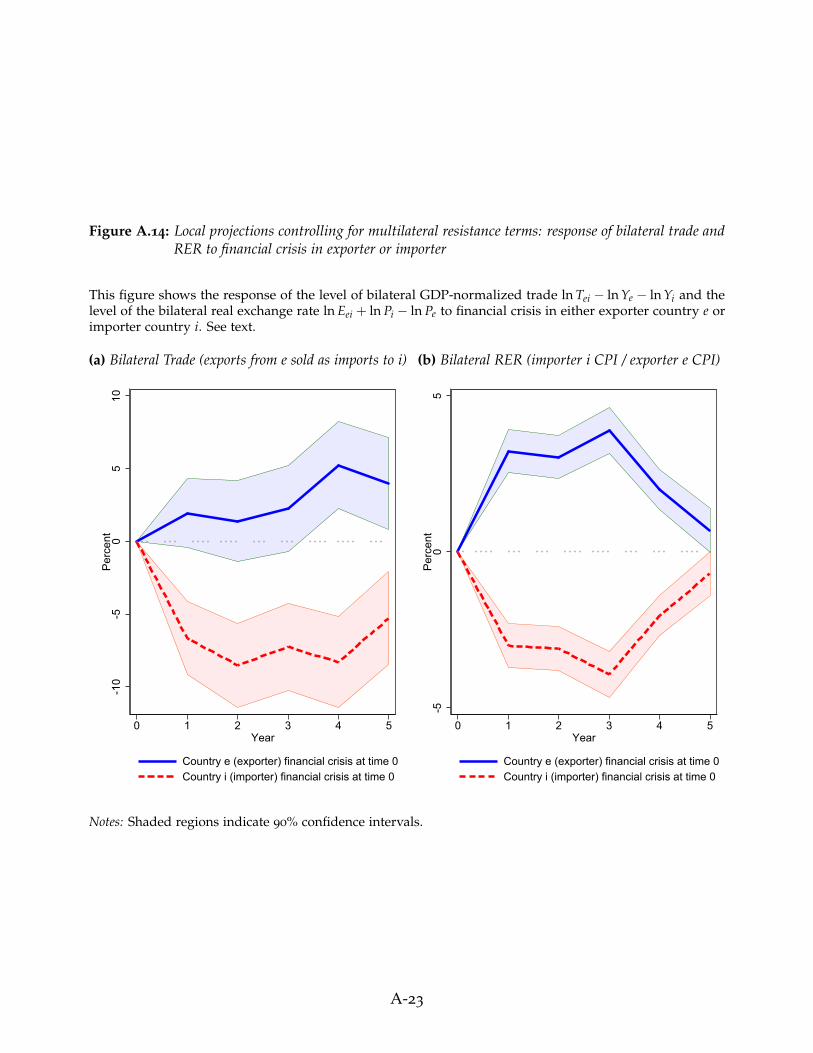
Figure A.14: Local projections controlling for multilateral resistance terms: response of bilateral trade andRER to financial crisis in exporter or importer
This figure shows the response of the level of bilateral GDP-normalized trade ln Tei − ln Ye − ln Yi and thelevel of the bilateral real exchange rate ln Eei + ln Pi − ln Pe to financial crisis in either exporter country e orimporter country i. See text.
(a) Bilateral Trade (exports from e sold as imports to i)
-10
-50
510
Per
cent
0 1 2 3 4 5Year
Country e (exporter) financial crisis at time 0Country i (importer) financial crisis at time 0
(b) Bilateral RER (importer i CPI / exporter e CPI)
-50
5P
erce
nt
0 1 2 3 4 5Year
Country e (exporter) financial crisis at time 0Country i (importer) financial crisis at time 0
Notes: Shaded regions indicate 90% confidence intervals.
A-23
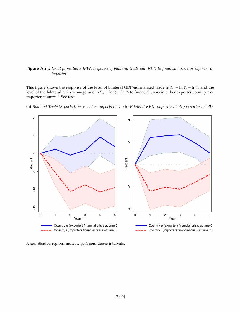
Figure A.15: Local projections IPW: response of bilateral trade and RER to financial crisis in exporter orimporter
This figure shows the response of the level of bilateral GDP-normalized trade ln Tei − ln Ye − ln Yi and thelevel of the bilateral real exchange rate ln Eei + ln Pi − ln Pe to financial crisis in either exporter country e orimporter country i. See text.
(a) Bilateral Trade (exports from e sold as imports to i)
-15
-10
-50
510
Per
cent
0 1 2 3 4 5Year
Country e (exporter) financial crisis at time 0Country i (importer) financial crisis at time 0
(b) Bilateral RER (importer i CPI / exporter e CPI)
-4-2
02
4P
erce
nt
0 1 2 3 4 5Year
Country e (exporter) financial crisis at time 0Country i (importer) financial crisis at time 0
Notes: Shaded regions indicate 90% confidence intervals.
A-24
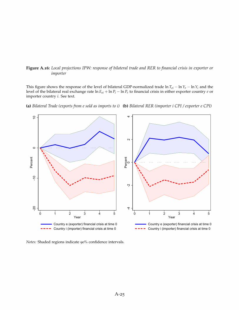
Figure A.16: Local projections IPW: response of bilateral trade and RER to financial crisis in exporter orimporter
This figure shows the response of the level of bilateral GDP-normalized trade ln Tei − ln Ye − ln Yi and thelevel of the bilateral real exchange rate ln Eei + ln Pi − ln Pe to financial crisis in either exporter country e orimporter country i. See text.
(a) Bilateral Trade (exports from e sold as imports to i)
-20
-10
010
Per
cent
0 1 2 3 4 5Year
Country e (exporter) financial crisis at time 0Country i (importer) financial crisis at time 0
(b) Bilateral RER (importer i CPI / exporter e CPI)
-4-2
02
4P
erce
nt
0 1 2 3 4 5Year
Country e (exporter) financial crisis at time 0Country i (importer) financial crisis at time 0
Notes: Shaded regions indicate 90% confidence intervals.
A-25
F. Response of Bilateral Trade Flows to Financial Crises:Additional Tables and Figures
This section includes the tables with estimates corresponding to figures 8, 9, 10 and 11 inSection 5 in the main text.
• Table A.6 shows the results of the estimation of equation 2 (for bilateral trade) splittingthe sample into subperiods. It corresponds to Figure 8 in the main text.
• Table A.7 shows the results of the estimation of equation 2 (for bilateral trade) splittingthe sample into groups according to the level of development of the exporter or theimporter. It corresponds to Figure 9 in the main text.
• Table A.8 shows the results of the estimation of equation 3 (for the bilateral RER)splitting the sample into subperiods. It corresponds to Figure 8 in the main text.
• Table A.9 shows the results of the estimation of equation 3 (for the bilateral RER)splitting the sample into into groups according to the level of development of theexporter or the importer. It corresponds to Figure 9 in the main text.
• Table A.10 shows the results of the estimation of equation 2 (for bilateral trade)controlling for various other types of crises and corresponds to the left panel in Figure11 in the main text.
• Table A.11 shows the results of the estimation of equation 3 (for the bilateral RER)controlling for various other types of crises and corresponds to the right panel inFigure 11 in the main text.
• Table A.14 shows the results of the estimation of equation 2 (for bilateral trade)separately for trade in final goods and intermediate inputs. and corresponds to Figure10 in the main text.
• Figure A.17 and Panel C in Table A.14 shows the results of the estimation of equation2 (for bilateral trade) separately for trade in capital goods.
A-26
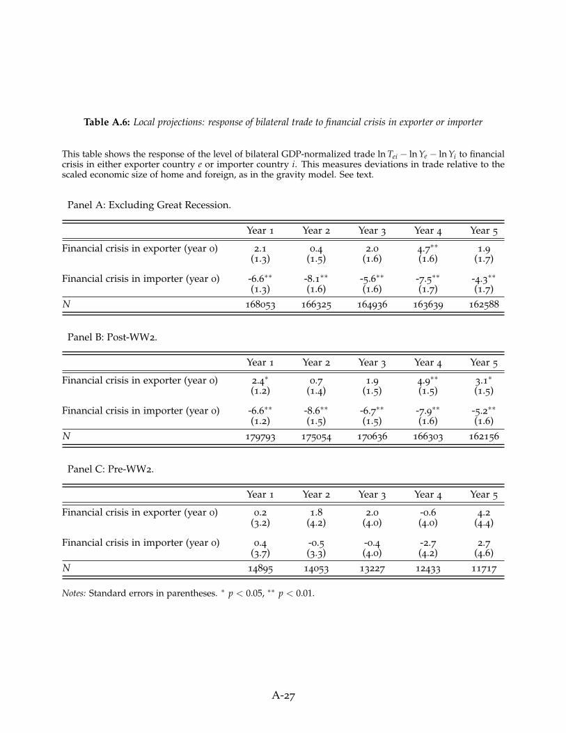
Table A.6: Local projections: response of bilateral trade to financial crisis in exporter or importer
This table shows the response of the level of bilateral GDP-normalized trade ln Tei − ln Ye − ln Yi to financialcrisis in either exporter country e or importer country i. This measures deviations in trade relative to thescaled economic size of home and foreign, as in the gravity model. See text.
Panel A: Excluding Great Recession.
Year 1 Year 2 Year 3 Year 4 Year 5
Financial crisis in exporter (year 0) 2.1 0.4 2.0 4.7∗∗ 1.9(1.3) (1.5) (1.6) (1.6) (1.7)
Financial crisis in importer (year 0) -6.6∗∗ -8.1∗∗ -5.6∗∗ -7.5∗∗ -4.3∗∗(1.3) (1.6) (1.6) (1.7) (1.7)
N 168053 166325 164936 163639 162588
Panel B: Post-WW2.
Year 1 Year 2 Year 3 Year 4 Year 5
Financial crisis in exporter (year 0) 2.4∗ 0.7 1.9 4.9∗∗ 3.1∗(1.2) (1.4) (1.5) (1.5) (1.5)
Financial crisis in importer (year 0) -6.6∗∗ -8.6∗∗ -6.7∗∗ -7.9∗∗ -5.2∗∗(1.2) (1.5) (1.5) (1.6) (1.6)
N 179793 175054 170636 166303 162156
Panel C: Pre-WW2.
Year 1 Year 2 Year 3 Year 4 Year 5
Financial crisis in exporter (year 0) 0.2 1.8 2.0 -0.6 4.2(3.2) (4.2) (4.0) (4.0) (4.4)
Financial crisis in importer (year 0) 0.4 -0.5 -0.4 -2.7 2.7(3.7) (3.3) (4.0) (4.2) (4.6)
N 14895 14053 13227 12433 11717
Notes: Standard errors in parentheses. ∗ p < 0.05, ∗∗ p < 0.01.
A-27
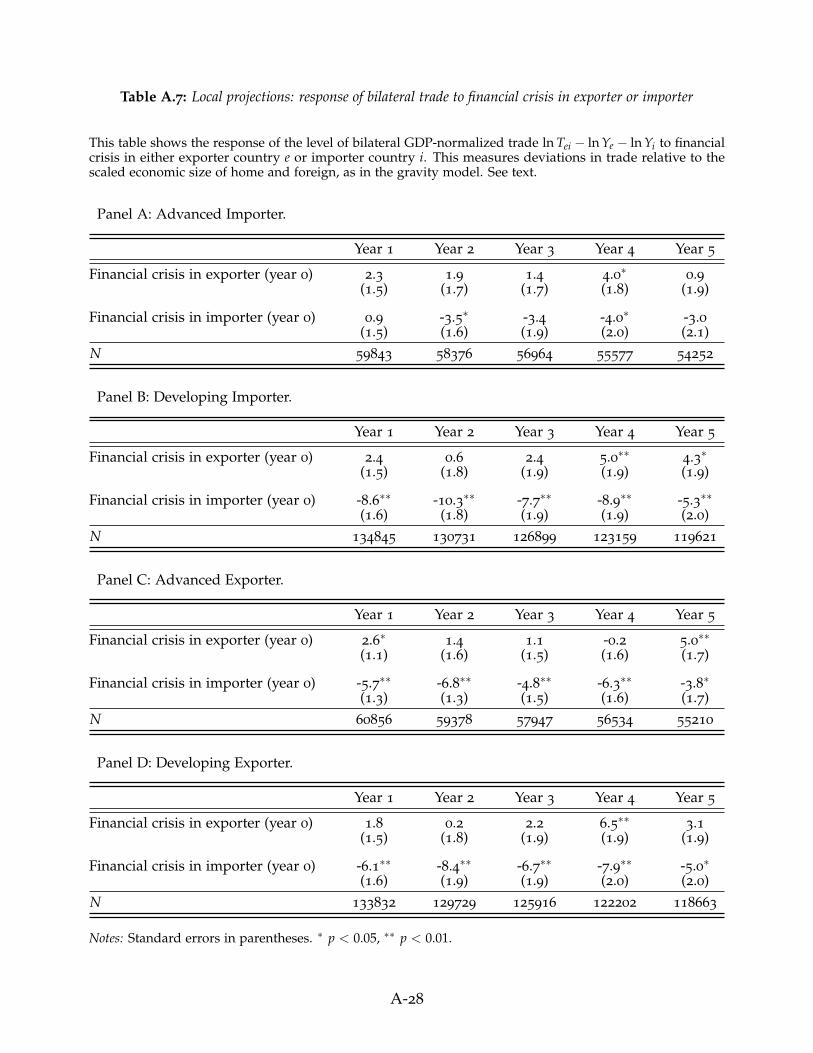
Table A.7: Local projections: response of bilateral trade to financial crisis in exporter or importer
This table shows the response of the level of bilateral GDP-normalized trade ln Tei − ln Ye − ln Yi to financialcrisis in either exporter country e or importer country i. This measures deviations in trade relative to thescaled economic size of home and foreign, as in the gravity model. See text.
Panel A: Advanced Importer.
Year 1 Year 2 Year 3 Year 4 Year 5
Financial crisis in exporter (year 0) 2.3 1.9 1.4 4.0∗ 0.9(1.5) (1.7) (1.7) (1.8) (1.9)
Financial crisis in importer (year 0) 0.9 -3.5∗ -3.4 -4.0∗ -3.0(1.5) (1.6) (1.9) (2.0) (2.1)
N 59843 58376 56964 55577 54252
Panel B: Developing Importer.
Year 1 Year 2 Year 3 Year 4 Year 5
Financial crisis in exporter (year 0) 2.4 0.6 2.4 5.0∗∗ 4.3∗(1.5) (1.8) (1.9) (1.9) (1.9)
Financial crisis in importer (year 0) -8.6∗∗ -10.3∗∗ -7.7∗∗ -8.9∗∗ -5.3∗∗(1.6) (1.8) (1.9) (1.9) (2.0)
N 134845 130731 126899 123159 119621
Panel C: Advanced Exporter.
Year 1 Year 2 Year 3 Year 4 Year 5
Financial crisis in exporter (year 0) 2.6∗ 1.4 1.1 -0.2 5.0∗∗(1.1) (1.6) (1.5) (1.6) (1.7)
Financial crisis in importer (year 0) -5.7∗∗ -6.8∗∗ -4.8∗∗ -6.3∗∗ -3.8∗(1.3) (1.3) (1.5) (1.6) (1.7)
N 60856 59378 57947 56534 55210
Panel D: Developing Exporter.
Year 1 Year 2 Year 3 Year 4 Year 5
Financial crisis in exporter (year 0) 1.8 0.2 2.2 6.5∗∗ 3.1(1.5) (1.8) (1.9) (1.9) (1.9)
Financial crisis in importer (year 0) -6.1∗∗ -8.4∗∗ -6.7∗∗ -7.9∗∗ -5.0∗(1.6) (1.9) (1.9) (2.0) (2.0)
N 133832 129729 125916 122202 118663
Notes: Standard errors in parentheses. ∗ p < 0.05, ∗∗ p < 0.01.
A-28
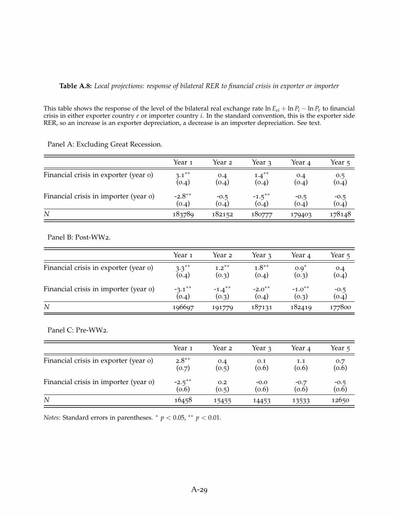
Table A.8: Local projections: response of bilateral RER to financial crisis in exporter or importer
This table shows the response of the level of the bilateral real exchange rate ln Eei + ln Pi − ln Pe to financialcrisis in either exporter country e or importer country i. In the standard convention, this is the exporter sideRER, so an increase is an exporter depreciation, a decrease is an importer depreciation. See text.
Panel A: Excluding Great Recession.
Year 1 Year 2 Year 3 Year 4 Year 5
Financial crisis in exporter (year 0) 3.1∗∗ 0.4 1.4∗∗ 0.4 0.5(0.4) (0.4) (0.4) (0.4) (0.4)
Financial crisis in importer (year 0) -2.8∗∗ -0.5 -1.5∗∗ -0.5 -0.5(0.4) (0.4) (0.4) (0.4) (0.4)
N 183789 182152 180777 179403 178148
Panel B: Post-WW2.
Year 1 Year 2 Year 3 Year 4 Year 5
Financial crisis in exporter (year 0) 3.3∗∗ 1.2∗∗ 1.8∗∗ 0.9∗ 0.4(0.4) (0.3) (0.4) (0.3) (0.4)
Financial crisis in importer (year 0) -3.1∗∗ -1.4∗∗ -2.0∗∗ -1.0∗∗ -0.5(0.4) (0.3) (0.4) (0.3) (0.4)
N 196697 191779 187131 182419 177800
Panel C: Pre-WW2.
Year 1 Year 2 Year 3 Year 4 Year 5
Financial crisis in exporter (year 0) 2.8∗∗ 0.4 0.1 1.1 0.7(0.7) (0.5) (0.6) (0.6) (0.6)
Financial crisis in importer (year 0) -2.5∗∗ 0.2 -0.0 -0.7 -0.5(0.6) (0.5) (0.6) (0.6) (0.6)
N 16458 15455 14453 13533 12650
Notes: Standard errors in parentheses. ∗ p < 0.05, ∗∗ p < 0.01.
A-29
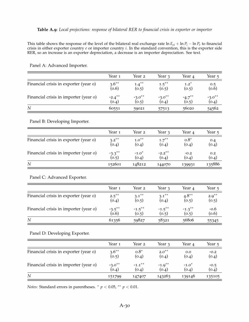
Table A.9: Local projections: response of bilateral RER to financial crisis in exporter or importer
This table shows the response of the level of the bilateral real exchange rate ln Eei + ln Pi − ln Pe to financialcrisis in either exporter country e or importer country i. In the standard convention, this is the exporter sideRER, so an increase is an exporter depreciation, a decrease is an importer depreciation. See text.
Panel A: Advanced Importer.
Year 1 Year 2 Year 3 Year 4 Year 5
Financial crisis in exporter (year 0) 3.6∗∗ 1.4∗∗ 1.5∗∗ 1.2∗ 0.5(0.6) (0.5) (0.5) (0.5) (0.6)
Financial crisis in importer (year 0) -2.4∗∗ -3.0∗∗ -3.0∗∗ -4.7∗∗ -3.0∗∗(0.4) (0.5) (0.4) (0.5) (0.4)
N 60551 59021 57513 56020 54562
Panel B: Developing Importer.
Year 1 Year 2 Year 3 Year 4 Year 5
Financial crisis in exporter (year 0) 3.2∗∗ 1.0∗∗ 1.7∗∗ 0.8∗ 0.4(0.4) (0.4) (0.4) (0.4) (0.4)
Financial crisis in importer (year 0) -3.3∗∗ -1.0∗ -2.2∗∗ -0.2 0.2(0.5) (0.4) (0.4) (0.4) (0.4)
N 152601 148212 144070 139931 135886
Panel C: Advanced Exporter.
Year 1 Year 2 Year 3 Year 4 Year 5
Financial crisis in exporter (year 0) 2.5∗∗ 3.1∗∗ 3.1∗∗ 4.8∗∗ 2.9∗∗(0.4) (0.5) (0.4) (0.5) (0.5)
Financial crisis in importer (year 0) -3.5∗∗ -1.5∗∗ -1.5∗∗ -1.3∗∗ -0.6(0.6) (0.5) (0.5) (0.5) (0.6)
N 61356 59827 58321 56806 55345
Panel D: Developing Exporter.
Year 1 Year 2 Year 3 Year 4 Year 5
Financial crisis in exporter (year 0) 3.6∗∗ 0.8∗ 2.0∗∗ 0.0 -0.2(0.5) (0.4) (0.4) (0.4) (0.4)
Financial crisis in importer (year 0) -3.0∗∗ -1.1∗∗ -1.9∗∗ -1.0∗ -0.5(0.4) (0.4) (0.4) (0.4) (0.4)
N 151799 147407 143263 139146 135105
Notes: Standard errors in parentheses. ∗ p < 0.05, ∗∗ p < 0.01.
A-30

Table A.10: Local projections controlling for other crises types: response of bilateral trade to financial crisisin exporter or importer
This table shows the response of the level of bilateral GDP-normalized trade ln Tei − ln Ye − ln Yi to financialcrisis in either exporter country e or importer country i. This measures deviations in trade relative to thescaled economic size of home and foreign, as in the gravity model. See text.
Year 1 Year 2 Year 3 Year 4 Year 5
Financial crisis in exporter (year 0) 1.6 0.2 2.7 3.4∗ 4.6∗∗
(1.1) (1.4) (1.5) (1.4) (1.5)
Financial crisis in importer (year 0) -7.5∗∗ -8.5∗∗ -7.0∗∗ -7.2∗∗ -5.7∗∗
(1.2) (1.3) (1.5) (1.5) (1.5)
N 136980 131861 125566 122269 119516
Notes: Standard errors in parentheses. ∗ p < 0.05, ∗∗ p < 0.01.
Table A.11: Local projections controlling for other crises types: response of bilateral RER to financial crisisin exporter or importer
This table shows the response of the level of the bilateral real exchange rate ln Eei + ln Pi − ln Pe to financialcrisis in either exporter country e or importer country i. In the standard convention, this is the exporter sideRER, so an increase is an exporter depreciation, a decrease is an importer depreciation. See text.
Year 1 Year 2 Year 3 Year 4 Year 5
Financial crisis in exporter (year 0) 3.9∗∗ 0.8∗ 2.5∗∗ 1.0∗∗ 1.1∗∗
(0.5) (0.3) (0.5) (0.4) (0.4)
Financial crisis in importer (year 0) -3.8∗∗ -0.8∗ -2.7∗∗ -1.1∗∗ -1.3∗∗
(0.5) (0.3) (0.5) (0.4) (0.4)
N 123604 119220 113242 110717 108639
Notes: Standard errors in parentheses. ∗ p < 0.05, ∗∗ p < 0.01.
A-31
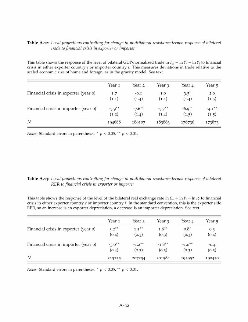
Table A.12: Local projections controlling for change in multilateral resistance terms: response of bilateraltrade to financial crisis in exporter or importer
This table shows the response of the level of bilateral GDP-normalized trade ln Tei − ln Ye − ln Yi to financialcrisis in either exporter country e or importer country i. This measures deviations in trade relative to thescaled economic size of home and foreign, as in the gravity model. See text.
Year 1 Year 2 Year 3 Year 4 Year 5
Financial crisis in exporter (year 0) 1.7 -0.1 1.0 3.5∗ 2.0(1.1) (1.4) (1.4) (1.4) (1.5)
Financial crisis in importer (year 0) -5.9∗∗ -7.6∗∗ -5.7∗∗ -6.9∗∗ -4.1∗∗
(1.2) (1.4) (1.4) (1.5) (1.5)
N 194688 189107 183863 178736 173873
Notes: Standard errors in parentheses. ∗ p < 0.05, ∗∗ p < 0.01.
Table A.13: Local projections controlling for change in multilateral resistance terms: response of bilateralRER to financial crisis in exporter or importer
This table shows the response of the level of the bilateral real exchange rate ln Eei + ln Pi − ln Pe to financialcrisis in either exporter country e or importer country i. In the standard convention, this is the exporter sideRER, so an increase is an exporter depreciation, a decrease is an importer depreciation. See text.
Year 1 Year 2 Year 3 Year 4 Year 5
Financial crisis in exporter (year 0) 3.2∗∗ 1.1∗∗ 1.6∗∗ 0.8∗ 0.3(0.4) (0.3) (0.3) (0.3) (0.4)
Financial crisis in importer (year 0) -3.0∗∗ -1.2∗∗ -1.8∗∗ -1.0∗∗ -0.4(0.4) (0.3) (0.3) (0.3) (0.3)
N 213155 207234 201584 195952 190450
Notes: Standard errors in parentheses. ∗ p < 0.05, ∗∗ p < 0.01.
A-32
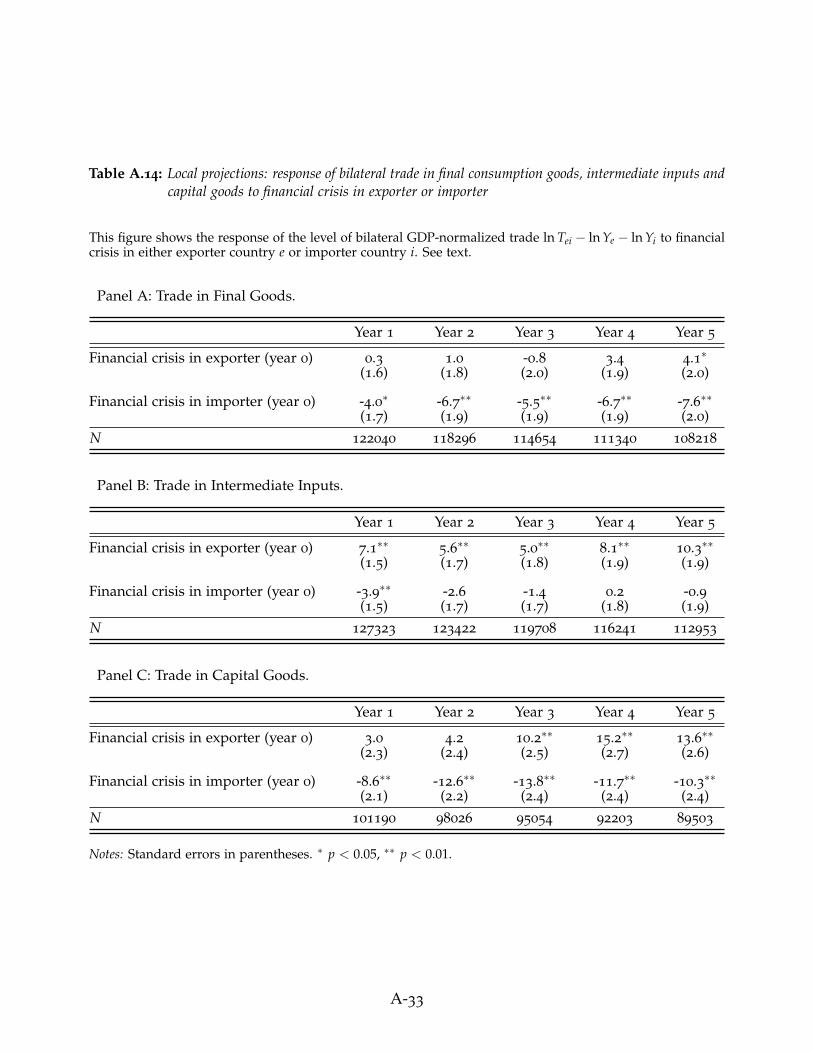
Table A.14: Local projections: response of bilateral trade in final consumption goods, intermediate inputs andcapital goods to financial crisis in exporter or importer
This figure shows the response of the level of bilateral GDP-normalized trade ln Tei − ln Ye − ln Yi to financialcrisis in either exporter country e or importer country i. See text.
Panel A: Trade in Final Goods.
Year 1 Year 2 Year 3 Year 4 Year 5
Financial crisis in exporter (year 0) 0.3 1.0 -0.8 3.4 4.1∗(1.6) (1.8) (2.0) (1.9) (2.0)
Financial crisis in importer (year 0) -4.0∗ -6.7∗∗ -5.5∗∗ -6.7∗∗ -7.6∗∗(1.7) (1.9) (1.9) (1.9) (2.0)
N 122040 118296 114654 111340 108218
Panel B: Trade in Intermediate Inputs.
Year 1 Year 2 Year 3 Year 4 Year 5
Financial crisis in exporter (year 0) 7.1∗∗ 5.6∗∗ 5.0∗∗ 8.1∗∗ 10.3∗∗(1.5) (1.7) (1.8) (1.9) (1.9)
Financial crisis in importer (year 0) -3.9∗∗ -2.6 -1.4 0.2 -0.9(1.5) (1.7) (1.7) (1.8) (1.9)
N 127323 123422 119708 116241 112953
Panel C: Trade in Capital Goods.
Year 1 Year 2 Year 3 Year 4 Year 5
Financial crisis in exporter (year 0) 3.0 4.2 10.2∗∗ 15.2∗∗ 13.6∗∗(2.3) (2.4) (2.5) (2.7) (2.6)
Financial crisis in importer (year 0) -8.6∗∗ -12.6∗∗ -13.8∗∗ -11.7∗∗ -10.3∗∗(2.1) (2.2) (2.4) (2.4) (2.4)
N 101190 98026 95054 92203 89503
Notes: Standard errors in parentheses. ∗ p < 0.05, ∗∗ p < 0.01.
A-33
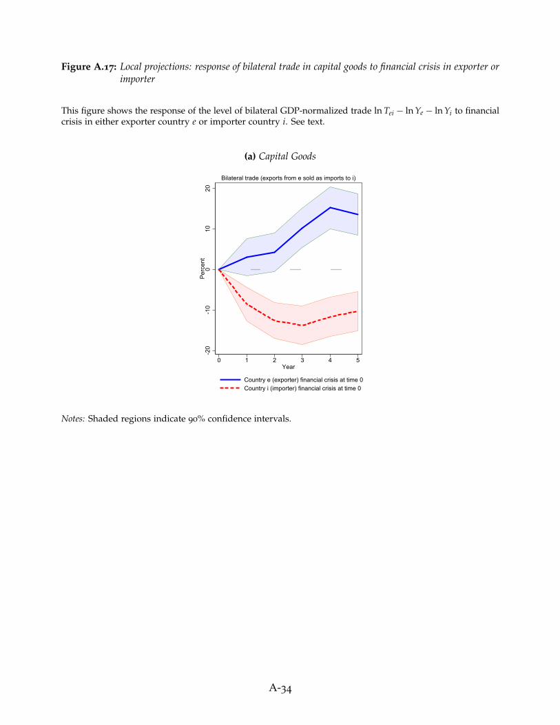
Figure A.17: Local projections: response of bilateral trade in capital goods to financial crisis in exporter orimporter
This figure shows the response of the level of bilateral GDP-normalized trade ln Tei − ln Ye − ln Yi to financialcrisis in either exporter country e or importer country i. See text.
(a) Capital Goods
-20
-10
010
20P
erce
nt
0 1 2 3 4 5Year
Country e (exporter) financial crisis at time 0Country i (importer) financial crisis at time 0
Bilateral trade (exports from e sold as imports to i)
Notes: Shaded regions indicate 90% confidence intervals.
A-34