AFRICAN ECONOMIC RESEARCH CONSORTIUM(AERC)

COLLABORATIVE MASTERS DEGREE PROGRAMME

(CMAP) IN ECONOMICS FOR ANGLOPHONE AFRICA

(EXCEPT NIGERIA)

JOINT FACILITY FOR ELECTIVES

MONETARY THEORY AND PRACTICE

LECTURE NOTES – PART 1

(July 2020)

2 of 373

Contents INTRODUCTION ........................................................................................................................................ 4

LEARNING OUTCOMES .......................................................................................................................... 4

1.1 INTRODUCTION: ISSUES IN MONETARY ECONOMICS ......................................................... 5

1.1.1 Definition; Functions and Evolution of Money ...................................................................... 5

1.1.2 The Role of Money in Macroeconomy ................................................................................ 29

1.1.3 Changing Paradigms in Monetary Theory .......................................................................... 33

1.2 THE DEMAND FOR MONEY .......................................................................................................... 38

1.2.1 Classical Approach to Demand for Money or Fisher’s Equation ................................... 39

1.2.2 Theories of Demand of Money: Baumol and Tobin-Markowitz Model .......................... 53

1.2.3 Friedman's Restatement of the Quantity Theory of Money ................................... 71

1.2.4 Microfoundations of Money: The Representative Agents (Households and

Firms) 76

1.2.5 The Demand for Money vis- a- viz the Demand for other Commodities .............. 80

1.2.6 Money in the Utility Functions .................................................................................... 81

1.2.7 Shopping-Time Models................................................................................................ 86

1.2.8 Cash-in-Advance Models (Clower Constraint)................................................................... 88

1.2.9 Overlapping Generation Model .................................................................................. 92

1.2.10 Currency Substitution .................................................................................................. 99

1.2.11 Empirical Studies of the Demand for Money with emphasis on Africa .............. 104

1.3 THE SUPPLY OF MONEY ............................................................................................................. 109

1.3.1 Money Supply/Stock (including the effects of Financial Innovations) ................ 110

1.3.2 Endogenous Money Supply: Credit Creation Process ......................................... 112

1.3.3 The Monetary Base Model of Money Supply ......................................................... 121

1.3.4 Flow of Funds Approach to Money Supply............................................................. 127

1.3.5 Fiscal Balance and the Money Supply Process .................................................... 133

1.3.6 Empirical Studies of Money Supply ......................................................................... 134

1.4 MONEY, PRICES AND EMPLOYMENT ............................................................................................ 145

1.4.1 Money and Theories of Inflation ............................................................................... 146

3 of 373

1.4.2 Monetary Control and Inflation ................................................................................. 155

1.4.3 Money Growth and Business Cycles....................................................................... 159

1.4.4 Expectations of the Real Business Cycle and Expected Inflation ...................... 163

1.4.5 Money and Employment............................................................................................ 167

1.5 CENTRAL BANKING AND MONETARY POLICY ................................................................ 176

1.5.1 A review of Objectives and Functions of the Central Bank .................................. 177

1.5.2 Monetary Policy Targets, Interest Rates Target, Inflation Target and Instruments

(Direct and Indirect) ....................................................................................................................... 193

1.5.3 Monetary Transmission Mechanism of Monetary Policy ...................................... 227

1.5.4 Interest Rates and Monetary Policy (Taylor’s Rule) ............................................. 239

1.5.5 Theories of Central Bank Independence and Time Consistency of Policies .... 245

1.5.6 Theoretical modelling of the role of Central Banks and monetary policy: The Three

Equation Model of Monetary Policy ............................................................................................. 260

1.5.7 Theory of interest Rates ............................................................................................ 275

1.5.8 Simple Vector Autoregressive (VAR) Models for Analyzing Monetary Policy ............ 314

1.5.9 Empirical Studies on Central Banking and Monetary Policy with Emphasis on

Africa. 320

1.6 MONEY IN THE OPEN ECONOMY ........................................................................................ 324

1.6.2 Money and BOP Adjustment .................................................................................... 345

1.6.3 Monetary Policy Under Alternative Exchange Rate Regimes ....................................... 354

1.6.4 The Policy Mix and Monetary Policy Coordination .......................................................... 369

4 of 373

INTRODUCTION

The purpose of this course is to enable you to acquire sufficient knowledge of monetary theory

and policy. The course content is designed to ensure that the state of the art of monetary theory is

given sufficient exposition, while at the same time introducing sufficient doses of policy and

empirical topics with special reference to developing countries, in particular African countries.

The course adequately prepares you for advanced research and practice in the area plus policy

analysis and implementation. As the course outline indicates, course is in two parts. Part I deals

with issues relating to various aspects of monetary theory including the role of money, money

demand, money supply, money and inflation, monetary management, and central banking as well

as money in the open economy. Part II covers the economics of financial institutions and

financial intermediation, relationship between financial development and economic growth,

money in an open economy, international financial institutions, and global economy. As well as

providing theoretical frameworks for analysing banking intermediations and the conduct of

monetary policy, the course will also present empirical evidence and policy actions wherever

possible to support the theories.

LEARNING OUTCOMES

Upon completion of this course, students should be able to:

Demonstrate an understanding of the subject matter and financial environments.

Narrate the main historical patterns of monetary thought and the diversity of ideas in monetary

economics; especially on the effectiveness of monetary policy and the contending schools in

monetary theories and policy;]

Appreciate the empirical relevance and validity, and intuitive understanding of the effect of

money on the aggregate economy;

Discuss the role of money in an economy from the perspective of both Classical and Keynesian

changing paradigms;

Appreciate the determination of prices including, inflation, interest rates, exchange rate, and

bond and share prices;

Explain theories underpinning demand and supply of money as well as the microfoundations of

money

Explain the theoretical and empirical implications of the conduct of monetary policy on the

macroeconomy.

5 of 373

Demonstrate an understanding of financial markets (such as those for bonds, stocks, and

exchange rates) and financial institutions such (banks, insurance companies, mutual funds, etc)

You should however note that the class notes provided in this course are no mean exhaustive.

Some additional required readings are provided in the course outline and many more may be

incorporated as the course proceeds. Assessment of this course will be based on continuous

assessment, practice exercises and final examination at a designated location and date. However,

at the end of each section are activities/questions/tasks, which you will be asked to complete to

demonstrate your understanding of the subject matter. Students are therefore strongly encouraged

to work through the practice exercises at the end of each section.

1.1 INTRODUCTION: ISSUES IN MONETARY ECONOMICS

In this first section in our lecture, we will focus on Money: Functions and Historical Evolution;

The Role of Money in the Macroeconomy; Changing Paradigms in Monetary Theory.

1.1.1 Definition; Functions and Evolution of Money

Money is a difficult concept to define in that it fulfills not only one function but several. The

definition of money in the literature is grouped into three strands, functional, theoretical or

traditional and empirical definitions. In what follows, we discuss each strand in detail.

Functional Definition of Money

The functional definition of money is lead by Prof. Coulbourn who defines money as a means of

valuation and of payment in terms of the unit of account and exchange1. This is very wide. It

includes cheques, gold, coin, etc., so long as it can perform the functions of valuation and

payment. Sir John Hides (1967) says that money is defined by it functions. Anything is money

which is used as money, implying in simple terms, Money is what money does.

Some have defined money based on the legal terms. Anything backed by law to be accepted by

everyone for payment is called money.

Let’s take a minute then to go through some of the primary and secondary functions of money

before we discuss the theoretical definition of money.

1 Coulbourn, Macroeconomic Theory, McGraw-Hill, New York, 1963

6 of 373

Primary Functions of Money

The two primary functions of money are to act as a medium of exchange/payment and as a unit

of account.

(i) Money as a Medium of Exchange/Payment.

This function was traditionally called the medium of exchange. According to Handa (2009), in a

modern context however, in which transactions can be conducted with credit cards, it is better to

refer to it as the medium of (final) payments. This is the primary function of money because all

the other functions of money are developed from this function. By serving as a medium of

payment, money revokes the need for double coincidence of wants and the inconveniences and

difficulties associated with barter (which we discuss later in this lecture). As a medium of

payment, money acts as an intermediary. It makes exchange possible. It helps production

indirectly through specialization and division of labour which, in turn, increase efficiency and

output. According to Prof. Walters, money, therefore, serves as a ‘factor of production, enabling

output to increase and diversify. Money also facilitates trade. When acting as the intermediary,

it helps one good or service to be traded indirectly for others.

(ii) Money as Unit of Account

The second primary function of money is to act as a unit of account. Money is the standard for

measuring value just as the yard or meter is the standard for measuring length. The monetary

unit measures and expresses the values of all goods and services. In fact, the monetary unit

expresses the value of each good or service in terms of price. Money is the common

denominator which determines the rate of exchange between goods and services which are

priced in terms of the monetary unit. There can be no pricing process without a measure of

value. As a matter of fact, measuring the values of goods and services in the monetary unit

facilitates the problem of measuring the exchange values of goods in the market. When values

are expressed in terms of money, the number of prices is reduced from n (n-1) in barter economy

to (n – 1) in monetary economy. Money as a unit of account also facilitates accounting. “Assets

of all kinds, liabilities of all kinds, income of all kinds, and expenses of all kinds can be stated in

terms of common monetary units to be added or subtracted.”

7 of 373

Secondary Functions of Money

Money performs three other secondary functions: as a standard of deferred payments, as a store

of value, and a transfer of value. These are discussed below

Money as a Store of Value: Another secondary function of money is to act as a store of value.

The commodity chosen as money is always something which can be kept for long periods

without deterioration or wastage. It is a form in which wealth can be kept intact from one year to

the next. Money is a bridge from the present to the future. It is therefore essential that the

money commodity should always be one which can be easily and wisely stored. Obviously, we

know money is not the only store of value. This function can be served by any valuable asset.

One can store value for the future by holding short-term promissory notes, bonds, mortgages,

preferred stocks, household furniture, houses, land, or any other kind of valuable goods. The

principal advantages of these other assets as a store of value are that they, unlike money,

ordinarily yield an income in the form of interest, profits, rent or usefulness. And they sometimes

rise in value in terms of money. On the other hand, they have certain disadvantages as a store of

value, among which are the following: (1) They sometimes involve storage costs; (2) they may

depreciate in terms of money; and (3) they are “illiquid” in varying degrees, for they are not

generally acceptable as money and it may be possible to convert them into money quickly only

by suffering a loss of value.”

Money as a Standard of Deferred Payments. The third function of money is to act as a standard

of deferred or postponed payments. All debts are taken in money. It was easy under barter to

take loans in goats or grains but difficult to make repayments in such perishable commodities in

the future. Money has simplified both the taking and repayment of loans because the unit of

account is durable.

Contingent Functions of Money

Also called the incidental functions. The contingent functions are based on traditional functions

(primary & secondary), made possible by Prof David Kinsley. He outlined the functions as;

1. Money as the most liquid of all assets.

Wealth can be in the form of bonds, debentures, etc. There is an opposite direction- meaning

that money can be turned into the other forms of wealth and the other forms of wealth can also

be turned into money. Savings can be kept in securities. Money aids the functions of liquidity.

2. Money is the basis of the credit system.

Behind or underneath every credit is money. Credit creation can expand money supply through

money multiplier. Whatever credit one receives, one pays/receives it back in money (Cash).

8 of 373

Money has helped in the formation of capital or money market. These are based on the fact that

money performs the function of unit of account.

3. It brings about the equalization of marginal utility and productivity. Within the indifference

curve analysis, where MUx = λPx, given the Px and λ marginal utility of good x (MUx) can be

estimated. It also helps in estimating the productivity of a firm and how much to pay for wages,

W of labour based on marginal productivity of labour (MPL). i.e. W = MPL. But MPL

determines the productivity of a labour. Therefore, given wages of the individual, the MPL can

be measured in the perfect market.

4. Measurement of National Income

The National income (Y) couldn’t have been possible to be calculated in the barter system. But

with the use of money, it is easy to estimate the total income, Y of a country to determine the

country’s welfare. It also helps in calculating the GDP.

5. In the distribution of National Income

Rewards to the factors of production in the form of wages, rent, interest and profit are all

determined and paid with money.

Theoretical Definition of Money

In 1962, Prof, Johnson in his book ‘Monetary Theory and Policy’ gave four different schools of

thought with regards to the definition of money.

The traditional definition of money is also known as the view of the currency school. The

traditional definition of money defines money as currency and deposits or chequables. That is

money is a medium of exchange. Thus almost 100% liquid. Keynes in his General Theory

followed the traditional view and defined money as currency and demand deposits. Hicks in his

Critical Essays in Monetary Theory points towards a threefold traditional classification of the

nature of money: thus to act as a unit of account (or measure of value as Wicksell puts it), as a

means of payment and as a store of value. The Banking School criticized the traditional

definition of money as arbitrary. This view sees the meaning of money as very narrow because

there are other assets which are equally acceptable as media of exchange. These include time

deposits of commercial banks, commercial bills of exchange, etc

Other schools of thought like the banking school said that the definition is narrow because it

includes other things that money can do and that there are other assets which are equally

acceptable as medium of exchange. Examples include, time deposits, drafts bonds which are

sometimes used as money. By ignoring these assets, the traditional view is not in a position to

9 of 373

analyse their influence in increasing their velocity. Furthermore, by excluding them from the

definition of money, the Keynesians place greater emphasis on the interest elasticity of the

demand function for money. Empirically, they forged a link between the stock of money and

output via the rate of interest. We present the detailed position of classical and Keynesian

economists below

According to classical economists money is just a medium of exchange and it cannot influence

the income and employment of a country. In other words, the money supply which is in

circulation just performs the function of exchange of goods and services. People keep money

with themselves so that they could transact goods and services. Thus, according to them money

is just a token and it has nothing to do with economic activity of a country. They further say that

money is like a veil which wraps the goods and services in itself. Money has been accorded as a

veil because it has camouflaged the operation of real economic forces. Classical economists do

not rule out the act of savings or borrowing. They think the savings, borrowings and lendings

take place under the shield of a veil. It means that they have attached the problems of savings,

borrowings and lendings with the transactive motive of holding money. Whether any body

purchases the goods or services or borrows, both are similar functions. The funds are borrowed

or lent with the help of money but they do not influence the economic activity in any way. In this

respect, Adam Smith writes:

"Money is like a road which helps in transporting the goods and services produced in a country

to the market, but this road does not itself produce any thing".

"Accord money like an agent which expedites the chemical action of any process, but it can not

change the components of chemical action".

Thus, classical economists are of the view, that money facilitates the transaction of goods and

services, but it does not influence the quantity of goods and services in any way. It means that

money cannot influence the real variables like production, income and employment. It can only

influence the monetary variables like monetary wages and prices. In other words, if the supply of

money in a country is increased the income and employment will remain unaffected. The

increase in supply of money will lead to increase the prices, hence monetary wages. When prices

and wages increase in the same proportion real wages will remain the same. As a result, the

employment and output will remain the same.

All above discussion shows that the ideology that money cannot influence economy was a corner

stone of classical economics. This philosophy remained popular till before and after World War

I. But when classical utopia of nonintervention collapsed during 1970's depression the concept of

money as a veil disappeared and money was accorded a dynamic element. AH the problems

which emerged during 1930's were attributed to money. Because of this reason, "Money was

10 of 373

accorded Evil Genius". The money which got the importance by putting to an end the problems

of barter system, was later on accorded as veil and finally it was held responsible for inflation

and deflation.

According to Keynesian Economists money has another role to play which is as a store of

value. They said that due to this role of money a link is established between present and future.

And because of this role money can influence the economic activity, level of income and

employment. Quite against classical neutrality of money, Keynes thinks that money can alter the

level of income and employment of an economy. Classical economists had integrated both the

real and monetary sectors of the economy. But Keynes clearly bifurcated the monetary and real

sectors of the economy. They said that in monetary sector rate of interest is determined by

demand for money and supply of money. However, They stressed upon demand for money while

the demand for money rises for two motives: (i) Transactive Demand for Money and (ii)

Speculative Demand for Money.

The transaction demand for money depends upon income levels of the people. While speculative

demand for money depends upon rate of interest. The speculative demand for money is

concerned with money as a store of value. Thus, according to Keynes money is not just

demanded for transaction purposes but it is also demanded to take advantage by the liquidity of

money. In addition to monetary sector, Keynes also presented their views regarding real sector.

They said that equilibrium level of national income is determined where aggregate demand is

equal to aggregate supply. They said that it is not necessary that equilibrium level of national

income will be determined at the level of full employment. Rather equilibrium level of national

income may be at full employment, may be at below full employment and may be at above full

employment.

Below full employment represents deflation while above full employment represents inflation.

Both inflation and unemployment are undesirable. Therefore, to remove them state will have to

interfere with fiscal and monetary policies. All this means that according to Keynes money can

be used to change the level of income and employment. In this respect, he establishes a

relationship between real and monetary sectors of the economy. As if supply of money is

increased the rate of interest will decrease. Hence investment .national income and employment

will be boosted up removing unemployment. Moreover, through fiscal action by printing new

notes or borrowing from banks govt. can initiate public works program. They will also have the

effect of removing the unemployment. All this shows that in Keynes economics money can

influence the level of employment.

Turning to the definition of money according to Friedman or Monetarists which has also being

described as the modern definition of Money or the Chicago school of thought, the scope of

11 of 373

money is much broader than the traditional definitions. In his book “ Employment, growth and

price”, Freidman (1959) defined money literally as the number of dollars people carry around in

their pockets as well as the number of dollars they have to their credit at banks in the form of

demand deposits and time deposit. In effect, he defines money as currency plus all adjusted

deposits in commercial banks. He extended his definition to time deposits-you notify the bank

before one can withdraw. Usually time deposit is not included when classifying liquid assets.

However, this definition is criticized as being too narrow since in most empirical studies the

definition of money goes beyond time and demand deposits because of sophistications in

financial transactions.

Based on this criticism, Freidman reframed his definition of money as “Any asset capable of

serving as a temporally abode of purchasing power” or anything that can serves as a purchasing

power or a means of buying.

The controversy didn’t end there. Many scholars still criticized this definition and Friedman was

compelled to restate that the definition of money shouldn’t be based on theory but how useful it

is. The monetarists which are known as modern friends of classical economists have much more

similarity regarding different issues. However, they also differ in certain fields. In connection

with money monetarists say: "Money Matters Very Much". This means that according to

monetarists money in an economy plays a very vital role. They say that aggregate expenditures

of the economy are influenced by the changes in the rate of interest As a result, the level of

income and employment can be affected. But it is confined to just short run. In case of long run

there is always existing a natural rate of unemployment. It means that whenever through easy

fiscal and monetary policies aggregate demand is increased, the level of unemployment will

come down. But whenever aggregate demand is controlled prices will be stabilized, but economy

will experience the same level of unemployment which the economy faced before increase in

aggregate demand.

There are also other well acceptable definitions in the literature such as The Radcliff Definition

and The Gurley –Shaw (1960) Definition. The former is actually the outcome of the committees

set up to work on the Money system. The report of the committee defined money as notes plus

bank deposits. This includes only those assets that are commonly used as a medium of exchange.

The bank deposits included demand and time deposits. Even though we can use other things as

money, their convertibility requires extra cost. Theirs is a quite different from Radcliff. They

regard a substantial volume of liquid assets held by financial intermediaries and the liabilities of

non-bank financial intermediaries as close substitutes for money. NBFIs do not perform the

functions of bank but rather intermediates.

12 of 373

Evolution of Money

Money dates back several centuries in the era of the Indo-European civilisation. Well before the

invention of minted coins in the Lydian cities of the Aegean in the7th century BCE, writings

from the Sumerian civilisation at Ur in the 3rd millennium BCE refer to documents mentioning

silver struck with the head of Ishtar. The mother-goddess and symbol of fertility, Ishtar was also

the goddess of death. So from the very outset, money’s ambivalence reflects the ambiguity of its

social function: an instrument of cohesion and pacification in the community, it is also at the

centre of power struggles and a source of violence.

The word “money” is derived from the Latin word “Moneta” which was the surname of the

Roman Goddess of Juno in whose temple at Rome, money was coined. The origin of money is

seen in ancient times. Even the primitive era man had some sort of money. The type of money

in every age depended on the nature of its livelihood, the progress of human civilization at

different times and places. In a hunting society, the skins of wild animals were used as money.

The pastoral society used livestock, whereas the agricultural society used grains and foodstuffs

as money. The Greeks used coins as money. Let’s discuss how money has evolved from the

barter system to today.

Barter System

At the beginning, there was no money. Before the advent of money, the primitive economy was

engaged in exchange and trade but more directly without any medium of exchange. This is

known as the Barter system. People engaged in barter, the exchange of merchandise for

merchandise, without value equivalence.

Then, a person catching more fish than the

necessary for himself and his group,

exchanged his excess fish for the surplus of

another person who, for instance, had

planted and harvested more corn that what

he would need. This elementary form of

trade prevailed at the beginning of

civilization, and may be found today

among people of primitive economies, in

regions where difficult access makes

13 of 373

money scarce and, even in special

situations, where people barter items

without regard for their equivalence in

value. This is the case, for instance, of a

child who exchanges with his friend an

expensive toy for another of lesser value,

which it treasures.

Goods used in barter are generally in their natural state, in line with the environment conditions

and activities developed by the group, corresponding to elementary needs of the group’s

members. This exchange, however, is not free from difficulties, since there is not a common

measure of value among the items bartered.

Difficulties of the Barter System

The barter system as a method of exchange has the following disadvantages:

Lack of Double Coincidence of Wants. For an efficient functioning of the barter system, double

coincidence of wants was required on the part of those who wanted to exchange goods or

services. To be successful, the barter system involved multilateral transactions which are not

possible practically. Consequently, if the double coincidence of wants is not matched exactly, no

trade is possible under barter. Thus a barter system is time-consuming and was a great hindrance

to the development and expansion of trade.

Lack of a Common Measure of Value. Another difficulty under the barter system was the lack of

a common unit in which the value of goods and services should be measured.

Indivisibility of Certain Goods. The barter system was based on the exchange of goods with

other goods. It was difficult to fix exchange rates for certain goods which were indivisible.

Such indivisible goods pose a real problem under barter trade.

Difficulty in Storing Value. Under the barter system it was difficult to store value If someone

wanted to save real capital over a long period he/she would be faced with the difficulty that

during the period of storage, the commodity may become obsolete or deteriorate in value.

Difficulty in Making Deferred Payments. In a barter economy, it was difficult to make future

payments. As payments were made in goods and services, debt contracts were not possible due

to disagreements on the part of the two parties on the following grounds:

Lack of Specialization. Another difficulty of the barter system was that it was associated with a

production system where each person was a jack-of-all -trades. In other words, a high degree of

14 of 373

specialization was difficult to achieve under the barter system. Specialization and

interdependence in production was only possible in an expanded market system based on the

money economy. In this case no economic progress is possible in a barter economy due to lack

of specialization.

As a result of many difficulties and inconveniences in the barter system, around the globe there

was a need for accepted medium of exchange. With the passage of time many other types of

money emerged for the purpose of exchange. Following are the stages of evolution of money.

Commodity Money

Under commodity money, a large number of goods served as money, however the nature of

goods varied from time to time and place to place for example agricultural goods, birds, slaves

and animals etc. Some commodities, for their utility, came to be more sought than others are.

Accepted by all, they assumed the role of currency, circulating as an element of exchange for

other products and used to assess their value. This was the commodity money.

Cattle, mainly bovine, was one of the mostly used,

and had the advantages of moving for itself,

reproducing and rendering services, although there

was the risk of diseases and death.

Salt was another commodity money,

difficult to obtain, mainly in the interior

part of continents, also used as a

preservative for food. Both cattle and salt

left the marks in the Portuguese language

of their function as an exchange

instrument, as we keep using words such

as pecunia (money) and pecúlio

(accumulated money) derived from the

Latin work pecus (cattle). The word capital

(asset) comes from the Latin capita (head).

15 of 373

Similarly, the work salário (salary,

compensation, normally in money, due by

the employer for the services of an

employee) originates from the use of sal

[salt], in Rome, for payment of services

rendered.

Some African countries used, among other

commodity moneys, cowry – brought by

Africans –, wood, sugar, cocoa, tobacco and cloth,

exchanged in the 17th Century due to the almost

complete lack of money, traded in the form of yarn

balls, skeins and fabrics.

Later, commodities became inconvenient

for commercial trades, due to changes in

their values, the fact of being indivisible

and easily perishable, therefore checking

the accumulation of wealth.

In order to facilitate the exchange of goods, the commodity money also lost its popularity due to

the following reasons:

Lack of Storability

Lack of Divisibility

Lack of Durability

Lack of Transportability

Lack of Homogeneity

16 of 373

Lack of General Acceptability

Metal

The commodity money due to the above drawbacks was replaced by metallic money. As metals

were available from early times and were durable, portable and easily divisible therefore it got

rapid popularity. This was the era of un-coined metals wherein gold, silver, copper and other

metals were used as money. The popularity of metallic money is due to lack of homogeneity,

scarcity, to secure metals etc.

As soon as man discovered metal, it was used to made utensils and weapons previously made of

stone.

For its advantages, as the possibility of

treasuring, divisibility, easy of

transportation and beauty, metal became

the main standard of value. It was

exchanged under different forms. At the

beginning, metal was used in its natural

state, and later under the form of ingots

and, still, transformed into objects, from

rings to bracelets.

The metal so traded required weight assessment and assaying of its purity at each transaction.

Later, metal money gained definite form and weight, receiving a mark indicating its value,

indicating also the person responsible for its issue. This measure made transactions faster, as it

saved the trouble of weighing it and enabled prompt identification of the quantity of metal

offered for trade.

17 of 373

Money in the Form of Objects

Metal items came to be very valued

commodities.

As its production required, in addition to

knowledge of melting, knowing where the

metal could be found in nature, the task

was not at the reach of everyone.

The increased value of these objects led to

its use as money and the circulation as

money of small-scale replicas of metal

objects.

This is the case of the knife and key coins found in

the East and the talent, a copper or bronze coin

with the form of an animal skin that circulated in

Greece and Cyprus.

Ancient Coins

In the 7th century B.C. the first coins resembling current ones appeared: they were small metal

pieces, with fixed weight and value, and bearing an official seal, that is the mark of who has

minted them and also a guaranty of their value.

Gold and silver coins are minted in Greece, and small oval ingots are used in Lydia, made of a

gold and silver alloy called electrum.

18 of 373

Coins reflect the mentality of a people and their

time. One may find political, economic,

technological and cultural aspects in coins.

Through the impressions found in coins, we are

able to know the effigy of personalities who lived

centuries ago. Probably, the first historic character

to have his effigy registered in a coin was

Alexander the Great, of Macedonia, around the

year 330 B.C.

At the beginning, coin pieces were made by hand in a very coarse way, had irregular edges, and

were not absolutely equal to one another as today’s ones.

Gold, Silver and Copper

The first metals used in coinage were gold and silver. Employment of these metals happened for

their rarity, beauty, immunity to corrosion, economic value, and for old religious habits. In

primeval civilizations, Babylonian priests, knowledgeable about astronomy, taught to people the

close relationship between gold and the sun, silver and the moon. This led to a belief in the

magic power of such metals and of objects made with them.

Minting of gold and silver coins was common for

many centuries, and pieces were guaranteed by

their intrinsic value, that is to say, by the trade

value of the metal used in their production. Then, a

coin made with twenty grams of gold was

exchanged for goods of even value.

For many centuries, countries minted their most highly valued coins in gold, using silver and

copper for lesser value coins. This system was kept up to the end of the last century, when

cupronickel, and later other metallic alloys, became used, and coins came to circulate for their

extrinsic value, that is to say, for their face value, which is independent from their metal content.

With the appearance of paper money, minting of metal coins was restricted to lower values,

necessary as change. In this new role, durability became the most requested quality for coins.

Large quantities of modern alloys appeared, produced to support the high circulation of change

19 of 373

money.

Standardized Coinage

To make the process of exchange easier, the concept of standard coinage was adopted.

Government took control over all the coins. Coins were stamped with a logo, with uniform

weight and the value was guaranteed. These coins were standard as both their face and intrinsic

(value in themselves) were equal. Standardized coinage was unable to catch the minds due to

Too much time in extraction of metals from mines

Scarcity of Metals

Mobility

Paper Money

The emergence of paper money is a significant milestone in the evolution of money. In the

Middle Ages, the keeping of values with goldsmiths, persons trading with gold and silver items,

was common. The goldsmith, as a guaranty, delivered a receipt. With time, these receipts came

to be used to make payments, circulating from hand to hand, giving origin to paper money.

Some of had its value written by hand, as we today do with our checks.

With time, in the same form it happened with

coins, the government came to conduct the issue of

notes, controlling counterfeits and securing the

power to pay.

Currently, all countries have their central bank in

charge of issuing coins and notes.

Paper money experienced an evolution regarding the technique used in their printing. Today, the

printing of notes uses especially prepared paper and several printing processes, which are

complementary to each other, assuring to the final product a great margin of security and

durability conditions.

Different Shapes

Money has greatly changed its physical aspect along the centuries.

20 of 373

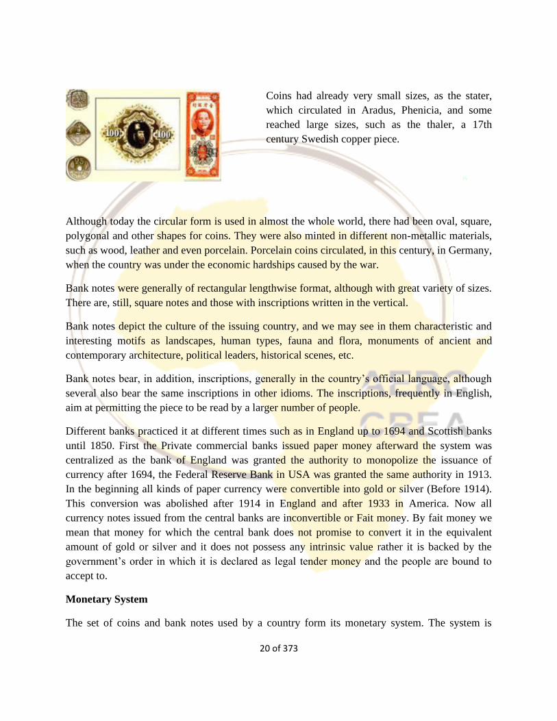
Coins had already very small sizes, as the stater,

which circulated in Aradus, Phenicia, and some

reached large sizes, such as the thaler, a 17th

century Swedish copper piece.

Although today the circular form is used in almost the whole world, there had been oval, square,

polygonal and other shapes for coins. They were also minted in different non-metallic materials,

such as wood, leather and even porcelain. Porcelain coins circulated, in this century, in Germany,

when the country was under the economic hardships caused by the war.

Bank notes were generally of rectangular lengthwise format, although with great variety of sizes.

There are, still, square notes and those with inscriptions written in the vertical.

Bank notes depict the culture of the issuing country, and we may see in them characteristic and

interesting motifs as landscapes, human types, fauna and flora, monuments of ancient and

contemporary architecture, political leaders, historical scenes, etc.

Bank notes bear, in addition, inscriptions, generally in the country’s official language, although

several also bear the same inscriptions in other idioms. The inscriptions, frequently in English,

aim at permitting the piece to be read by a larger number of people.

Different banks practiced it at different times such as in England up to 1694 and Scottish banks

until 1850. First the Private commercial banks issued paper money afterward the system was

centralized as the bank of England was granted the authority to monopolize the issuance of

currency after 1694, the Federal Reserve Bank in USA was granted the same authority in 1913.

In the beginning all kinds of paper currency were convertible into gold or silver (Before 1914).

This conversion was abolished after 1914 in England and after 1933 in America. Now all

currency notes issued from the central banks are inconvertible or Fait money. By fait money we

mean that money for which the central bank does not promise to convert it in the equivalent

amount of gold or silver and it does not possess any intrinsic value rather it is backed by the

government’s order in which it is declared as legal tender money and the people are bound to

accept to.

Monetary System

The set of coins and bank notes used by a country form its monetary system. The system is

21 of 373

regulated by appropriate legislation and organized from a monetary unit, its base value.

Currently almost all countries use a

monetary system of centesimal basis, in

which the coinage dividing the unit

represents one hundredth of its value.

Normally, higher values are expressed in notes while smaller values are represented by coins.

The current world trend is that daily expenses be paid with coins. Modern metallic alloys enable

coins to be more durable than notes, making them more appropriate to the intense use of money

as change.

The countries, through their central banks, control and guarantee the issue of money. The set of

notes and coins in circulation, the so called monetary mass, is constantly renewed through the

process of sanitation, substitution of worn out and torn notes

Near Money: Cheques

As coins and notes ceased to be convertible into precious metal, money became more

dematerialized and assumed abstract forms.

One of these forms is the cheque that, for simplicity of use and security offered, is being adopted

by an increasing number of people in their day-by-day activities.

This document, by which one orders

payment of a certain amount to its bearer

or to a person mentioned in it, aims mainly

at transactions with bank deposits.

Cheque is basically a representation of a particular amount and hence cannot be treated as legal

tender or high-powered money.

The important role played today in the economy by this form of payment is due to the

innumerable advantages offered by it, speeding transactions with large sums, avoiding hoarding

22 of 373

and diminishing the need of change by being a document completed by hand in the necessary

amount.

Money, whatever the form it has, is not valuable for itself, but for the goods and services it may

purchase. It is a sort of security giving its bearer the faculty of being creditor of society and take

advantage, through his or her purchasing power, of all conquests of modern man.

Money was not, hence, invented by a stroke of genius, but stemmed from a need, and its

evolution reflects, at each time, the willingness of man to harmonize its monetary instrument to

the reality of its economy.

Near Money

The next stage in the evolution of money has been the use of bills of exchange, treasury bills,

bonds, debentures, savings certificates, etc. They are known as “near money.” They are close

substitutes for money and are liquid assets. Thus, in the final stage of its evolution money has

become intangible. Its ownership is now transferable simply by book entry.

Electronic Money

Until now it is the last stage of evolution of money, this is the age of computer, now-a-days

people avoid using cash and even cheques in their financial matters. Besides the credit money,

they have now the facility of transferring money electronically which is quite effective in the

context of time saving and safety. The introduction of electric payments technology as a means

of transacting business has not only substituted for cheques but also for cash as well in the form

of electronic money (e-money). E-money is the form of money that exists in electronic form. All

kinds of debt cards, credit cards, ATM cards and smart cards are the examples of electronic

money. Electronic money is not legal tender money.

In most advanced countries the use of debit and credit cards are becoming more popular than the

use of cash in transacting a business. The ATM card is an example of a credit card that enables

the customer of a bank to withdraw money from his account without going to the bank itself.

The smart card (for example, the e-zwich in Ghana) is a type of store- value card that contains a

computer chip at allows it to be loaded with digital cash from the owner’s bank account

whenever needed. Smart cards can be loaded from ATM machines, personal computers with a

smart card reader or special type of phones. The e-cash is another form of electronic money used

on the internet to make purchases of goods and services. This process of making transfers online

and paying bills online is termed as internet banking.

Some of the things that are required for widening the use of e-cards include:

Electricity

23 of 373

Telecommunication infrastructure, for example internet facilities

A literate population in ICT-population that can use the internet

Efficient ICT support system capable of preventing internet fraud

Easy access to computers

Other forms of e-money that have emerged in recent times are money are mobile money and

digital currency

Mobile Money

Mobile money is an electronic wallet service or a movement of value that is made from a mobile

wallet, accrues to a mobile wallet, and/or is initiated using a mobile phone. Mobile payment on

the other hand is a movement of value that is made from a mobile wallet, accrues to a mobile

wallet, and/or is initiated using a mobile phone. Sometimes, the term mobile payment is used to

describe only transfers to pay for goods or services, either at the point of sale (retail) or remotely

(bill payments). Mobile wallet is an account that is primarily accessed using a mobile phone.

This is available in many countries and allows users to store, send, and receive money using their

mobile phone. The safe and easy electronic payments make. Mobile money a popular alternative

to bank accounts. It can be used on both smartphones and basic feature phones.

Digital Currency

Digital currency (digital money, electronic money or electronic currency) is a balance or a record

stored in a distributed database on the Internet, in an electronic computer database, within digital

files or within a stored-value card.[1] Examples of digital currencies include cryptocurrencies,

virtual currencies, central bank digital currencies and e-Cash.

Digital currencies exhibit properties similar to other currencies, but do not have a physical form

of banknotes and coins. Not having a physical form, they allow for nearly instantaneous

transactions. Usually not issued by a governmental body, virtual currencies are not considered a

legal tender and they enable ownership transfer across governmental borders

You can do almost anything online, including paying others with digital currency, currency that's

not held in physical form. Some hold no real value except within a certain community such as

the coins used in the game FarmVille. Others, such as the Bitcoin, do have real world value. As

of fall 2017, 1 Bitcoin is worth about $4800 US dollars.

24 of 373

Digital currency is code with monetary value and is backed by software

Forms

There are two major forms of digital currency.

Virtual currency is digital currency that is used within a specific community. For example, all

FarmVille players have access to the in-game virtual currency coins with which they can

purchase items for their farm. Virtual currency though is only valid within the specified

community. You can't take your FarmVille coins and use them to buy a hamburger from

McDonald's, therefore, it has no real world value.

Cryptocurrency, on the other hand, is digital currency that does have real world value, like

Bitcoin. This type of digital currency is based on mathematical algorithms with tokens being

transferred electronically over the internet via peer-to-peer networking.

A benefit to cryptocurrency is that it is not tied into the economy of any one country. This form

is decentralised and does not rely on any one regulatory agency. This means that if the economy

of one country crashes, your digital currency will remain the same.

With no regulatory agencies to go through, cryptocurrency makes it easier to conduct

international transactions. It can also be exchanged for any type of physical currency. And it is

completely private. Though transactions are digitally confirmed, they are anonymous. Your

personal details are never attached to your transactions, so there is no money trail as there is with

some physical currency.

Transactions are also irreversible. You know how if you deposit a fake check, the bank will then

reverse that transaction and take that money back out of your account? This can't happen in

cryptocurrency. There is little room for mistakes as all transactions are conducted via complex

algorithms that transfer tokens from one person to another.

25 of 373

Though all this privacy is usually considered a good thing, cryptocurrency has also been used for

illegal transactions such as money laundering and purchasing illegal drugs. It has also been

connected with ransomware, which is when a virus hijacks your computer and demands payment

in cryptocurrency to release your data.

Types

While there are only two forms of digital currency, there are actually many types.

There are as many types of virtual currencies as there are communities that have them. Virtual

currencies typically cannot be traded or exchanged with each other. You can't trade or exchange

FarmVille currency for Diner Dash currency. Each is only valid in its own gaming community or

app. There are many different cryptocurrencies to choose from as well. Some are accepted at

more places than others, but the most popular is currently Bitcoin. Right now, you can use your

Bitcoins to make purchases at Overstock.com, Expedia, eBay, Shopify, Etsy, DISH Network,

and Microsoft.

When you shop with Bitcoins, you'll actually be spending satoshis, which is the smallest fraction

of Bitcoin (at least for now). 1 Bitcoin is equal to 100,000,000 satoshis.

In addition to Bitcoins, Overstock also accepts all major alt-coins, other cryptocurrencies created

after the Bitcoin. The Bitcoin is still number 1 as far as cryptocurrencies are concerned. The

other major cryptocurrencies include Litecoin (launched in 2011), Ripple (launched in 2012),

Dash (launched in 2014), Monero (launched in 2014), and Ethereum (launched in 2015),

Mobile Digital Wallets

A number of electronic money systems use contactless payment transfer in order to facilitate

easy payment and give the payee more confidence in not letting go of their electronic wallet

during the transaction.

In 1994 Mondex and National Westminster Bank provided an "electronic purse" to residents of

Swindon

In about 2005 Telefónica and BBVA Bank launched a payment system in Spain called Mobipay,

which used simple short message service facilities of feature phones intended for pay-as-you-go

services including taxis and pre-pay phone recharges via a BBVA current bank account debit.

In January 2010, Venmo launched as a mobile payment system through SMS, which transformed

into a social app where friends can pay each other for minor expenses like a cup of coffee, rent

and pay a share of the restaurant bill when one has forgotten their wallet. It is popular with

college students, but has some security issues. It can be linked to a bank account, credit/debit

26 of 373

card or have a loaded value to limit the amount of loss in case of a security breach. Credit cards

and non-major debit cards incur a 3% processing fee.

On 19 September 2011, Google Wallet released in the United States to make it easy to carry all

one's credit/debit cards on a phone.

In 2012 Ireland's O2 (owned by Telefónica) launched Easytrip to pay road tolls which were

charged to the mobile phone account or prepay credit.

The UK's O2 invented O2 Wallet[27] at about the same time. The wallet can be charged with

regular bank accounts or cards and discharged by participating retailers using a technique known

as 'money messages'. The service closed in 2014.

On 9 September 2014, Apple Pay was announced at the iPhone 6 event. In October 2014 it was

released as an update to work on iPhone 6 and Apple Watch. It is very similar to Google Wallet,

but for Apple devices only.

Empirical and Econometric Developments on the Definition of Money

This section is based on Handa (2009) where we trace the historical definition and classification

of money. Numerous theoretical and empirical studies in the 1950s and 1960s pointed out the

development of close substitutes for money as a feature of the financial evolution of economies.

By the 1960s, these developments led to a realignment of the functional definition of money to

stress its store of value aspect, in this case as an asset relative to other assets, rather than medium

of payments aspect. The result of this shift in focus was to further stress the closeness of

substitution between the liabilities of banks and those of other financial intermediaries. Such

shifts in the definition of money were supported both by shifts in the analysis of the demand for

money, suited to the stress on the store-of-value function, and by a large number of empirical

studies. However, in the presence of a variety of assets performing the functions of money to

varying degrees, purely theoretical analysis did not prove to be a clear guide to the empirical

definition or measurement of money. As a result, research on measuring the money stock for

empirical and policy purposes took a variety of routes after the 1960s. Several broad routes may

be distinguished in this empirical work. Two of these were:

One of the routes was to measure money as the sum of M1 and those assets that are close

substitutes for demand deposits. Closeness of substitution was determined on the basis of the

price and cross-price elasticities in the money-demand functions or of the elasticities of

substitution between M1 and various non-money assets. Such studies, generally reported

27 of 373

relatively high degrees of substitution among M1, savings deposits in commercial banks, and

deposits in near-bank financial intermediaries and therefore supported a definition of money that

is broader than M1 and in many studies even broader than M2.

The second major mode of defining money was to examine its appropriateness in a

macroeconomic framework. In this approach, the definition of money was specified as that

which would “best” explain or predict the course of nominal national income and of other

relevant macroeconomic variables over time. But there proved to be little agreement on what

these other relevant variables should be. The quantity theory tradition (in the work of Milton

Friedman, most of his associates and many other economists) took nominal national income as

the only relevant variable. For the 1950s and 1960s, this approach found that the “best”

definition of money, as shown by examining the correlation coefficients between various

definitions of money and nominal national income, was currency in the hands of the public plus

deposits (including time) in the commercial banks. This was the Friedman definition of money

and was widely used in the 1960s. However, it should be obvious that the appropriate definition

of money under Friedman’s procedure could vary between periods and countries, as it did in the

1970s and 1980s.

Further, in the disputes on this issue in the 1960s, many researchers in the Keynesian tradition

took the appropriate macroeconomic variables related to money as being nominal national

income and an interest rate, and defined money much more broadly than M2 to include deposits

in several types of non-bank financial intermediaries and various types of Treasury bills and

government bonds. Up to the 1970s, empirical work along the above lines brought out an array

of results, conflicting in detail though often in agreement that M2 or a still wider definition of

money performs better in explaining the relevant macroeconomic variables than money narrowly

defined. This consensus vanished in the 1970s and 1980s in the face of increasing empirical

evidence that none of the simple-sum aggregates of money – whether M1, M2 or a still broader

one – had a stable relationship with nominal national income. Research on the 1970s and 1980s

data showed that (a) the demand functions for the various simple-sum monetary aggregates were

unstable, and (b) they did not possess a stable relationship with nominal

income.

The above findings for the simple sum aggregates prompted the espousal of several new

functional forms for the definition of money. The search for stability of the money-demand

function also led to refinement of econometric techniques, resulting in cointegration analysis and

28 of 373

error-correction modeling of non-stationary time series data, and the derivation of separate long-

run and short-run demand functions for money. Further, the continuing empirical instability of

the demand functions for M2 and still broader definitions of money since the 1980s led to an

increased preference for some form of M1 over broader aggregates for policy formulation and

estimation, thereby reversing the shift towards M2 and other broad monetary aggregates which

had occurred in the 1950s and 1960s. Further, the empirical instability of money-demand

functions led to a marked decrease after the 1980s in both analytical and empirical studies on the

definition of money. In addition, after the 1980s, at the monetary policy and macroeconomic

level, many central banks and researchers have chosen to focus on the interest rate as the

appropriate monetary policy instrument – thereby relegating money supply and demand to the

sidelines of macroeconomic reasoning.

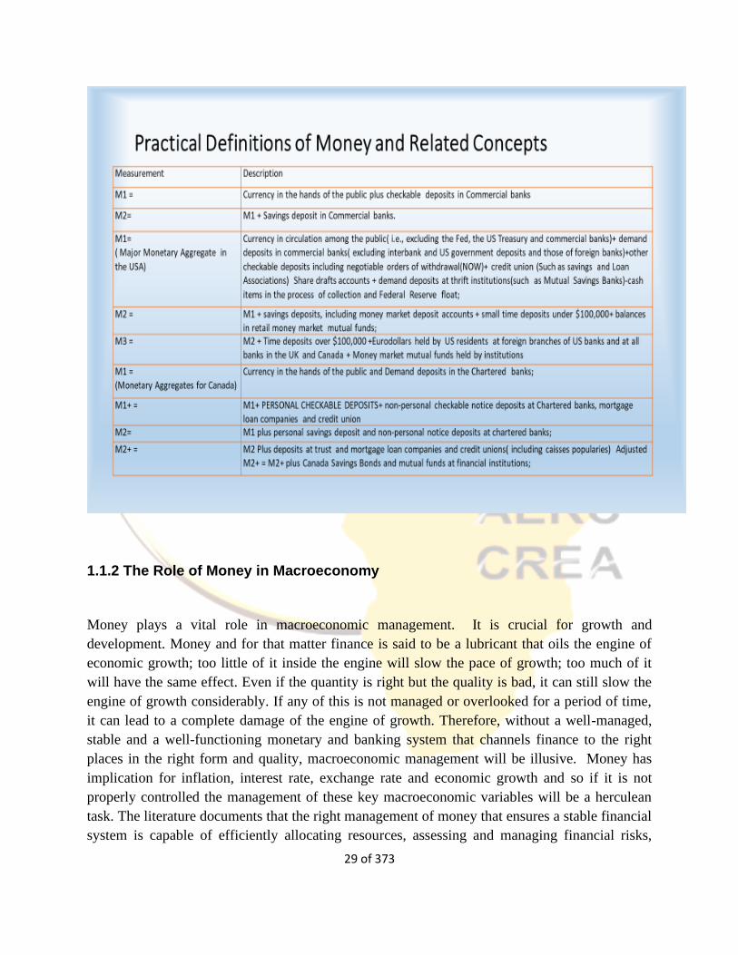
Practical Definitions of Money and Related Concepts

We have already referred to several definitions of money. These definitions are fairly, though

not completely, standardized across countries for M1 and M2 but tend to differ for broader

designations. The generic definitions of these monetary variables can be taken to be as

follows:

• M1= Currency in the hands of the public + checkable deposits in commercial banks;

• M2= M1 + savings deposits in commercial banks.

These generic definitions are modified to suit the context of different countries and their

central banks. Further, in general, with increases in the substitutability of different monetary

assets, the definitions of each of the aggregates have broadened over time. Often, the variations

in the definition of M1 are accommodated by using terms such as M1, M1+, M1++, etc.

29 of 373

1.1.2 The Role of Money in Macroeconomy

Money plays a vital role in macroeconomic management. It is crucial for growth and

development. Money and for that matter finance is said to be a lubricant that oils the engine of

economic growth; too little of it inside the engine will slow the pace of growth; too much of it

will have the same effect. Even if the quantity is right but the quality is bad, it can still slow the

engine of growth considerably. If any of this is not managed or overlooked for a period of time,

it can lead to a complete damage of the engine of growth. Therefore, without a well-managed,

stable and a well-functioning monetary and banking system that channels finance to the right

places in the right form and quality, macroeconomic management will be illusive. Money has

implication for inflation, interest rate, exchange rate and economic growth and so if it is not

properly controlled the management of these key macroeconomic variables will be a herculean

task. The literature documents that the right management of money that ensures a stable financial

system is capable of efficiently allocating resources, assessing and managing financial risks,

30 of 373

maintaining employment levels close to the economy’s natural rate, and eliminating relative

price movements of real or financial assets that will affect monetary stability, or economic

growth and employment levels (Beck et al., 2007 and World Bank 2016).

Fundamentally, there are 2 main forms in which the role of money can be classified- Static role

and Dynamic role.

Static role: This role emerges from the traditional functions of money, which we have discussed

previously.

Dynamic role: In its dynamic role, Money plays an important part in the lives of people and in

the economic system as a whole.

a) Role of money to the consumer. It makes the consumer sovereign because the consumer has

the power to choose. It also ensures effective demand. It brings about postponement of

consumption. The consumer’s income is in the form of money.

b) To the producer. It helps in calculating revenue, cost, and profit. It also aids in planning,

forecasting and budgeting. It brought about specialization and division of labour and how much

to pay each skills according to the marginal product (MP).

c) It brought about capital formation by transferring saving into investment. Money has made it

possible for people to save usually for a long time and earn interest on their savings. Investment

is also linked closely with the growth of the economy. Increasing investment increases the

income base of the economy just because money goes around in the economy.

d) As an index of economic growth, National income, income per capita and GDP are all

measured in terms of money. When the value of money falls, prices increase and this may arise

from too much money in the economy. Money is the index of an economy. If the value of money

increases, it means the economy is getting well the general price levels.

e) It has helped in solving the central problems in economic system- what to produce, how to

produce and to whom to produce. When the producer knows the MC, supply which is positively

linked with prices (money) gives incentive to the producer to produce where the prices are high

31 of 373

(P> MC). Feasibility studies help in identifying the income levels of the people in that

community, how to produce? to whom to produce? who is the target?, what transport system to

use?, whether the market is bases on a centralized government or market forces?, the Cost

Benefit Analysis (CBA) of the labour or capital intensive used, and whether distribution is

dependent on equity or on the survival of the fittest.

f) Facilitates the collection of taxes and subsidies as well as fostering income distribution.

It facilitates exchange of goods and services and helps in carrying on trade smoothly. The present

highly complicated economic system will not exist without money.

g) Money helps in maximising consumers’ satisfaction and producers’ profit. It helps and

promotes saving.

Other Things Money Does are as Follows:

Money promotes specialisation which increases productivity and efficiency.

It facilitates planning of both production and consumption.

Money can be utilised in reviving the economy from depression.

Money enables production to take place in advance of consumption.

It is the institution of money which has proved a valuable social instrument of promoting

economic welfare. The whole economic science is based on money; economic motives and

activities are measured by money.

Defects of Money

The classical regard money as a veil or wrapper without performing any function. It is simply a

tool of convenience to facilitate the exchange of goods and services but it is not a determinant of

the quantities produced. It does not bring any increase in output. Here are some of the defects of

money.

1. Money brings about instability in the value of money. E.g. excess supply of money wouldn’t

be too much of importance to the economy. Too much of it reduces its value.

32 of 373

When the value of money falls, it means the general price level of the economy increases. This is

what is called inflation. When inflation increases, money is less effective to perform its function

as a store of value. Investment also falls because inflation distorts the price level. An investor

will hold on with the investment because of the instable nature of the value of money.

The real value of goods and services might be falling because of inflation. If investors are

uncertain about the economy and the price level, they will not invest. These brings about unequal

distribution of income. Inflation or fall in the value of money causes direct and immediate

damage to creditors and consumers. On the contrary deflation or rise in the value of money

brings down the level of output, employment and income. If prices fall, production also falls

(depression). The effect of it is laying off some workers who lose their labour income,

employment rate increases, effective demand falls and price also falls. However, production

actually increases in the stable economy, but the two extreme ends (inflation and deflation) are

not good for the economy.

2. Money spreads monopoly.

Too much money leads to concentrating of capital in the hands of few capitalists who practice

monopoly and exploits both consumers and workers.

3. Wastage of resources

Because money is the basis of credit, too much credit to the individuals who might give to a

productive sector will create over capitalization, over production and this wastes output in the

system. If the individual decides not to give it to the productin sector but to the unproductive

sector, it is in itself wastage of resources. Especially, where there is political patronage without

easily assessing the use of money.

4. Black Money

Money being the store of value usually causes people to hand it. This happens when people

conceal money in order to evade tax. This works through money laundry where money does not

perform any activity. It creates an underground economy or black marketing where tax evasion is

rife. When you conceal money and refuse to pay tax on that money for a log time, it creates

black money. Transferring the black money is called money laundering and this leads to

underground or parallel economy.

33 of 373

5. Money creates a class economy which brings about conflict and distinguishes the rich from the

poor.

6. Cyclical fluctuation in money brings about over production where the economic activities

increase. This increases demand.

The defects of money discussed above are economic in nature. But there are some defects which

are non-economic. One non-economic defect of money is increase in crime rate. “The love of

money is the root of most evil”. In most cases, the moral, social and political fibers of the society

are brought down because of money. The resultant effects are corruption, political bankruptcy,

political instability, prostitution, strike actions, artificiality in religion which breeds fake pastors.

People deceive and betray their fellow human beings, take or give bribe to temper justice just

because of money. It is not getting the money which is not good but the attitude towards money.

Money is the lubricant for the smooth functioning of the economy. But the attitude of the various

economic agents (government, firms, individuals) is what is worrying.

1.1.3 Changing Paradigms in Monetary Theory

Broadly, there are two main school of thought of investigating monetary issues: Classical and

Keynesian group of models.

Classical group of models: This group of models argue the neutrality of money in the economy.

The main arguments are premised on perfect competition and market clearances.

Keynesian group of models: Here, they believe in non-neutrality of money at least in the short-

run. They argue that the economy is embedded with some rigidities that brings

about market distortions. The Keynesian paradigm recognizes that the economy may sometimes

have equilibrium in all markets, but does not assert that this occurs always or most of the time.

They believe that even if there is equilibrium, it may not be the competitive equilibrium. These

characteristics make money non-neutral.

34 of 373

Classical Models

Traditional Classical ideas: These include models that existed prior to Keynes’s publication of

The General Theory in 1936. The relevant theories are the quantity theory of money for the

determination of prices and the loanable funds theory for the determination of interest rates, Says

Law.

Neoclassical model Here, classical ideas are re-branded in the

post-General Theory period in a new compact into the IS-LM framework. The

re-branding included the elucidation of some nuances of the traditional classical ideas, such as

the wealth/Pigou and real balance effects, and addition of new elements such as the speculative

demand for money and the explicit analysis of the

commodity market at the macroeconomic level. Also, elements such as the quantity theory, the

loanable funds theory, Say’s law were discarded in this framework.

Monetarism: The short-run version of this model did not assume full employment and did not

imply continuous full employment in the economy. It is a hybrid between the classical and the

Keynesian paradigms, and made the switch away from Keynesian on claim of fiscal policy

efficacy. In its long-run version, it belonged in the classical paradigm.

Modern classical model This is a statement of the classical paradigm under the assumptions,

among others, of continuous labour market clearance even in the short-run. Also, it extends the

neoclassical model by the introduction of uncertainty and rational expectations.

New Classical Model: The new classical model imposes the assumption of Ricardian

equivalence on the modern classical

model. This assumption is an aspect of intertemporal rationality and the Jeffersonian

(democratic) notion that the government is nothing more than a representative of its electorate

and is regarded as such by the public in making the decisions on its own consumption

Keynesian Models

The Keynesian paradigm focuses on the deviations from the general equilibrium of the

competitive economy based on assumption of nominal wage rigidity. There can be a variety of

reasons for such deviations, requiring different models for their explanations.

Deviation from equilibrium could occur even when nominal wage is fully flexible

IS{LM analysis assumes that the central bank uses the money supply rather than the interest rate

as the monetary policy instrument and sets its level exogenously. However, the LM

equation/curve, and therefore the IS{LM analysis, is inappropriate for the macroeconomic

analysis of economies in which the central bank sets the interest rate exogenously. The more

appropriate analysis for such economies is the IS{IRT one.

35 of 373

In the short-run, money and credit are not neutral in real-world economies. They are neutral in

the analytical long

Neo-Keynesian Models

Just as Keynes posited his theory in response to gaps in classical economic analysis, Neo-

Keynesianism derives from observed differences between Keynes's theoretical postulations and

real economic phenomena. The Neo-Keynesian theory was articulated and developed mainly in

the U.S. during the post-war period. Neo-Keynesians did not place as heavy an emphasis on the

concept of full employment but instead focused on economic growth and stability.

The reasons the Neo-Keynesians identified that the market was not self-regulating were

manifold. First, monopolies may exist, which means the market is not competitive in a pure

sense. This also means that certain companies have discretionary powers to set prices and may

not wish to lower or raise prices during periods of fluctuations to meet demands from the public.

Labor markets are also imperfect. Second, trade unions and other companies may act according

to individual circumstances, resulting in a stagnation in wages that does not reflect the actual

conditions of the economy. Third, real interest rates may depart from natural interest rates as

monetary authorities adjust the rates to avoid temporary instability in the macroeconomy.

The two major areas of microeconomics by Neo-Keynesians are price rigidity and wage rigidity.

In the 1960s, Neo-Keynesianism began to examine the microeconomic foundations that the

macroeconomy depended on more closely. This led to a more integrated examination of the

dynamic relationship between microeconomics and macroeconomics, which are two separate but

interdependent strands of analysis.

The two major areas of microeconomics, which may significantly impact the macroeconomy as

identified by Neo-Keynesians, are price rigidity and wage rigidity. Both of these concepts

intertwine with social theory negating the pure theoretical models of classical Keynesianism.

For instance, in the case of wage rigidity, as well as influence from trade unions (which have

varying degrees of success), managers may find it difficult to convince workers to take wage cuts

on the basis that it will minimize unemployment, as workers may be more concerned about their

own economic circumstances than more abstract principles. Lowering wages may also reduce

productivity and morale, leading to overall lower output.

New Keynesian economics is a school of contemporary macroeconomics that strives to provide

microeconomic foundations for Keynesian economics. It developed partly as a response to

criticisms of Keynesian macroeconomics by adherents of new classical macroeconomics.

36 of 373

Two main assumptions define the New Keynesian approach to macroeconomics. Like the New

Classical approach, New Keynesian macroeconomic analysis usually assumes that households

and firms have rational expectations. However, the two schools differ in that New Keynesian

analysis usually assumes a variety of market failures. In particular, New Keynesians assume that

there is imperfect competition[1] in price and wage setting to help explain why prices and wages

can become "sticky", which means they do not adjust instantaneously to changes in economic

conditions.

Wage and price stickiness, and the other market failures present in New Keynesian models,

imply that the economy may fail to attain full employment. Therefore, New Keynesians argue

that macroeconomic stabilization by the government (using fiscal policy) and the central bank

(using monetary policy) can lead to a more efficient macroeconomic outcome than a laissez faire

policy would.

Activity 1.1: Review and discussion questions

If money lubricates the wheels of the economy, does it mean that money is always good?

“Our first step must be to elucidate more clearly the functions of money. ... Money, it is well

known, serves two principal purposes. By acting as a money of account, it facilitates exchanges

without its being necessary that it should ever itself come into the picture as a substantive object.

In this respect it is a convenience which is devoid of significance or real influence. In the second

place, it is a store of wealth. So we are told, without a smile on the face. But in the world of

classical economy, what an insane use to which to put it! For it is recognized characteristically of

money as a store of wealth that it is barren: whereas practically every other form of storing

wealth yields some interest or profit. Why should anyone outside a lunatic asylum wish to use

money as a store of wealth?” (Quarterly Journal of Economics, February 1937, pp.215-216).

Critically evaluate the above passage within the frameworks of Keynesian and Classical

Theorists of money functions.

What are the different ways of defining money in your economy? Compare these with

the monetary aggregates commonly used in another selected country. Explain their differences

and the reasons for such differentiation.

37 of 373

What are the underlying themes (or theme, if only one) of the classical paradigm? How

are they represented in the different models within this paradigm?

Explain the various models within the classical approach and compare them. Which

would you accept for your economy?

“The modern classical approach does not assume full employment. In fact, it allows for the

deviations of employment from its full-employment level.” Discuss these statements. If you

agree with them, what is the nature of such deviations? Compare their nature with the nature of

deviations from full employment that can occur in the traditional classical and neoclassical

approaches and in the 1970s monetarist doctrines.

What are the underlying themes of the Keynesian paradigm? Do they justify the study of just one

model, one variety of models, or several different varieties of models? Why?

“The 1970s monetarism was a hybrid between the classical and the Keynesian paradigms.”

Discuss.

“Under the modern classical approach, there is no sensible role for demand management

policies in both the short-run and the long-run.” Why not? Discuss.

38 of 373

1.2 THE DEMAND FOR MONEY

Introduction

In this section, you will learn about the theory of demand for money, focusing on classical and

Keynes theories and the demand for money theories that followed. We will also focus on

microfoundations of money (representative agent models) including money in utility function,

cash-in-advance and overlapping generation models. Demand for money is a prominent issue in

macroeconomics due to the important role that money plays in the determination of the price

level, interest income. But first we should know the meaning of demand for money. In general,

the demand for money refers to how much assets individuals wish to hold in the form of money

(as opposed to illiquid physical assets.) It is sometimes referred to as liquidity preference. The

demand for money is related to income, interest rates and whether people prefer to hold

cash(money) or illiquid assets like money.

Further, demand for money arises from two important functions of money. The first is that

money acts as a medium of exchange and the second is a store of value. Thus, individuals and

businessman wish to hold money partly in cash and partly in the form of assets. Theoretically,

speaks, various schools of thought in economics define differently the demand for money. In-

fact, people’s demand for money is not for nominal money holdings but real money balances,

because if people are merely concerned with nominal money holdings irrespective of the price

level, they said to suffer from money illusion.

In the theory, till recently, there were three approaches to demand for money, namely,

transactions approach or Fisher’s quantity theory of money, cash balances approach or

Cambridge equation and, Keynes theory of liquidity preference. However, in recent years

Baumol, Tobin and Friedman also have put forward new theories of demand for money.

Learning Outcome

By the end of this lecture, you should be able to

explain and discuss the difference between the Classicals (Fischerian Approach)and Keynes

approach to demand for money

analyze and differentiate the Transaction approach from the Cambridge approach to money

demand.

.

39 of 373

analyze the main determinants of the speculative motive of holding money.

explain Baumol and Tobin-Markowitz Models of demand for money.

Discuss the four main propositions of the Monetarist system and the Friedman's Restatement of

the Quantity Theory of Money.

Compare and contrast the role of money in the Monetarist and Keynesian systems.

Explain the microfoundations of money and clearly discuss the following models:

The Demand for Money vis- a- viz the Demand for other Commodities

Money in the utility functions

Shopping-Time Models

Cash-in-Advance Models (Clower Constraint)

Overlapping Generation Model

Appreciate empirical studies of the demand for money with emphasis on Africa

1.2.1 Classical Approach to Demand for Money or Fisher’s Equation

The classical economists did not explicitly formulate demand for money theory, but their views

are inherent in the quantity theory of money. They considered only the medium of exchange

function of money as an important one i.e., money as a means of purchasing of goods &

services. The cash transactions approach was popularised by Irving Fisher of the USA in 1911,

in his book ‘Purchasing Power of Money’. Through his equation of exchange he made an attempt

to determine price level and value of money.

Symbolically, Fisher’s equation of exchange is written as under

M’V’+ MV = PT …………….(1)

Where M is the total quantity of money, M’ is the credit money, V & V’ is its velocity of

circulation of money and credit, ‘P’ is the price level and, ‘T’ is the total amount of goods and

services exchanged for money. This equation equates the demand for money (PT) to supply of

money (MV). As mentioned earlier, he made an attempt to determine price level and value of

money. Value of money is meant by purchasing power of money. In order to find out the effect

of the quantity of money on the price level or the value of money we write the equation as:

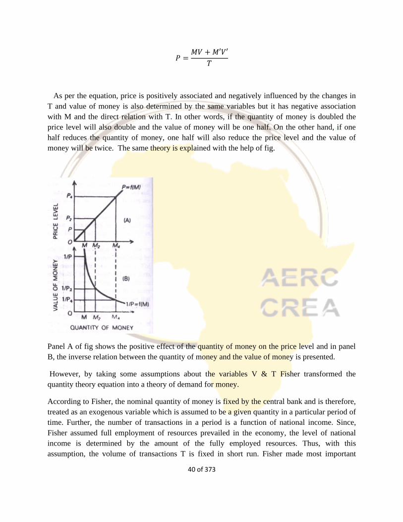
40 of 373

𝑃 =𝑀𝑉 + 𝑀′𝑉′

𝑇

As per the equation, price is positively associated and negatively influenced by the changes in

T and value of money is also determined by the same variables but it has negative association

with M and the direct relation with T. In other words, if the quantity of money is doubled the

price level will also double and the value of money will be one half. On the other hand, if one

half reduces the quantity of money, one half will also reduce the price level and the value of

money will be twice. The same theory is explained with the help of fig.

Panel A of fig shows the positive effect of the quantity of money on the price level and in panel

B, the inverse relation between the quantity of money and the value of money is presented.

However, by taking some assumptions about the variables V & T Fisher transformed the

quantity theory equation into a theory of demand for money.

According to Fisher, the nominal quantity of money is fixed by the central bank and is therefore,

treated as an exogenous variable which is assumed to be a given quantity in a particular period of

time. Further, the number of transactions in a period is a function of national income. Since,

Fisher assumed full employment of resources prevailed in the economy, the level of national

income is determined by the amount of the fully employed resources. Thus, with this

assumption, the volume of transactions T is fixed in short run. Fisher made most important

41 of 373

assumption which makes his equation as a theory of demand for money is that, velocity of

circulation (V) remains constant and is independent of M, P and T. this is because he thought

that velocity of circulation of money (V) is determined by institutional & technological factors

involved in the transaction process.

If we want to be in equilibrium, nominal quantity of money supply must be equal to the nominal

quantity of money demand. So that,

Ms = Md = M …………………………………..(2)

Where M is fixed by Central Bank.

With the above assumptions Fishers equation can be rewritten as

𝑀𝐷 =𝑃𝑇

𝑉 𝑜𝑟 𝑀𝐷 =

1.𝑃𝑇

𝑉…………………………….(3)

Therefore, according to Fisher, demand for money is depends on the following three factors: 1)

The number of Transactions 2) The average price transfers 3) The velocity of circulation of

money.

This approach is faced some serious difficulties in empirical research 1) in this approach

transactions are not only purchase of goods and services but also purchase of capital assets, so

that when there is a scope for frequent changes in capital assets, it is not appropriate to assume

that T will remain constant even if Y is taken to be constant due to full employment assumption

2) it is difficult to define and determine a general price level that covers not only current goods

and services but also capital assets.

The Cambridge Quantity Theory:

Cambridge cash balance theory of demand for money was put forward by Cambridge

economists, Marshall, Pigou, and Robertson. It places emphasis on the function of money as a

store of value or wealth instead of Fisher’s emphasis on the use of money as a medium of

exchange. Marshall, Pigou and Robertson focussed their analysis on the factors that determine

individual demand for holding cash balances. Although, they recognised that current interest

rate, wealth owned by the individuals, expectations of future prices and future rate of interest

determine the demand for money, they however believed that changes in these factors remain

constant or they are proportional to changes in individual’s income. Thus, they put forward a

view that individual’s demand for cash balances is proportional to the nominal income. Thus,

according to their approach, aggregate demand for money can be expressed as

𝑀𝑑 = 𝑘𝑃𝑌 …….1)

42 of 373

Where Y=real national income; P = average price level of currently produced goods and

services; PY = nominal income; k = proportion of nominal income (PY) that people want to hold

as cash balances

Demand for money in this equation is a linear function of nominal income. The slope of the

function is equal to k, that is, k = Md/Py, thus important feature of cash balance approach is that

it makes the demand for money as function of money income alone. A merit of this formulation

is that it makes the relation between demand for money and income as behavioural in sharp

contrast to Fisher’s approach in which demand for money was related to total transactions in a

mechanised manner.

We can observe the Cambridge approach even by the equations of individual economists.

Marshall’s formula is as follows:

𝑀 = 𝑘𝑌 … … … 2)

Where M is the quantity of money, Y is the total money income and K is the co-efficient whole

function is to bring the two sides into balance.

Pigou expresses the form of an equation as:

𝑃 = 𝐾𝑅

𝑀𝑜𝑟

𝑀

𝐾𝑅 ……………………..3)

Where P stands for the value of money or its inverse the price level (M/KR), M represents the

supply of money, R the total national income and K represents that fraction of R for which

people wish to keep cash.

Pigou presents the equation in an extended form by dividing cash into two parts: cash with the

public and, deposits which the people consider as cash, therefore:

𝑃 =𝐾𝑅

𝑀{𝐶 + ℎ(11 − 𝑐)}… … … … … … … … . .4)

Where, C denotes cash with the public (1-c) stands for bank deposits and H denotes the

percentage of cash reserve against bank deposits. If we assume the total amount of money in the

community as 1, the public as cash holds the public holds part of it and balance as deposits in

banks. Banks do not keep the entire deposits as cash only a portion or a part of it is kept as cash

43 of 373

and is denoted by ‘h’. Therefore, C+h (1-c) shows the amount of money in the economy at any

time denoting the proportion of cash and h(1-c) denoting it proportion of bank deposits.

Prof D H Roberstson’s equation is similar to that of Prof Pigou’s with a little difference.

Roberson’s equation is:

𝑀 = 𝑃𝐾𝑇 𝑜𝑟 𝑃 =𝑀

𝐾𝑇

Where P is the price level, T is the total amount of goods and services K represents the fraction

of T for which people wish to keep cash. Robertson’s equation is considered better than that of

Pigou as it is more comparable with that of Fisher. It is the best of all the Cambridge equations,

as it is the easiest.

Glay writes,’ Cambridge approach is conceptually richer than the transactions approach, the

former is incomplete because it does not formally incorporate the influence of economic

variables must mentioned on the demand for cash balances, Keynes attempted to eliminate this

shortcoming.

Another important feature of Cambridge demand for money function is that the demand for

money is proportional function of nominal income. Thus, it is proportional function of both price

level and real income. This implies tow things, first income elasticity of demand for money is

unity and secondly price elasticity of demand for money is also equal to unity so that any change

in the price level causes equal proportionate changes in the demand for money.

Policy implications of the quantity equation for persistently high rates of inflation

Rewrite the quantity equation in terms of growth rates as:

𝑀" + 𝑉" ≡ 𝑃" + 𝑦"

\

44 of 373

where ” indicates the rate of change (also called the growth rate) of the variable. This identity

can be restated as:

𝜋 ≡ 𝑀+V" − 𝑦"

where π is the rate of inflation and is the same as P”. This identity asserts that the rate of inflation

is always equal to the rate of money growth plus the growth rate of velocity less the growth rate

of output. Ceteris paribus, the higher the money growth rate, the higher will be the inflation rate,

whereas the higher the output growth rate is, the lower will be the inflation rate. Note that

velocity also changes over time and can contribute to inflation if it increases, or reduce inflation

when it falls. In normal circumstances in the economy, velocity changes during a year but not by

more than a few percentage points. Similarly, for most economies, real output growth rate is

usually only a few percentage points. For the quantity equation, we need only consider the

difference

(𝑉" − 𝑦") between them.

In the normal case, both velocity and output increase over time but the difference in their growth

rates is likely to be quite small, usually in low single digits. Adding this information to the

quantity equation implies that high (high single digits or higher numbers) and persistent (i.e. for

several years) rates of inflation can only stem from high and persistent money growth rates. This

is particularly true of hyperinflation in which the annual inflation rate may be in double (10

percent or more) or triple (100 percent or more) digits or even higher. Empirically, even at low

inflation rates, the correlation between money supply growth and inflation rates over long

periods is close to unity.

To reiterate, the source of inflation over long periods is usually money supply growth and

the source of persistently high inflation over even short periods is high and persistent money

growth rates. Therefore, if the monetary authorities wish to drastically reduce inflation rates

to low levels, they must pursue a policy that achieves an appropriate reduction in money supply

growth.

Keynes Liquidity Preference Approach

45 of 373

Keynes propounded a theory of demand for money in his general theory which occupies an

important place in his monetary theory. In other words, his demand for money is called liquidity

preference. How much of income or resources will a person hold in money and how much will a

person parts with or lend. Liquidity preference means the demand for money to hold or the desire

of the public to hold cash.

The term liquidity preference was first used by Keynes for to refer to the demand for money.

Keynes identified three reasons/motives for holding money in every economy. These motives

are:

(1) The transactions motive for holding money;

(2) The precautionary motive; and

(3) The speculative demand.

The Transactions Demand for Money

The transactions demand for money arises from the medium of exchange function of money.

This motive for holding money stems from the need to money for the current transactions of

personal and business exchange. To the individual, this motive relates to the need to hold money

to serve as s connection between the time of receipt of income and making of expenditures.

Similarly, to the businessman the motive is meant to bridge the gap between the time of

incurring business costs and the time of receipt of revenue from sales. If the time between the

making of expenditure and receipt of income is short then less money balances will be held by

the people for current transactions. If on the other hand, if the time between the incurring of

expenditure and receipt of income is long, more cash will be held by the people for day to day

transactions.

Changes may however occur in the transactions demand for money and may arise from changes

in individual and business expectations. Expectations in turn depend upon the level of income,

interest rates, the business turnover, the normal period between the receipt and disbursement of

income, etc. Given these factors, the transactions demand for money is a direct proportional and

positive function of the level of income, and is expressed as:

𝐿𝑇 = 𝑘𝑌

where

LT is the transactions demand for money (liquidity preference)

46 of 373

K is the proportion of income which is kept for transactions purposes, and

Y is income level.

Interest Rate and Transactions Demand

In recent years two renowned post-Keynesian economists, William J. Baumol and James Tobin’

have shown that there is some linkage between the transaction demand for money and the rate of

interest (we will treat this in detail in the subsequent section). They also demonstrated that this

relationship between transactions demand for money and income is not linear and proportional as

Keynes argued. Rather, changes in income lead to proportionately smaller changes in

transactions demand. This is because incomes received at the begging of the month is not spent

on the same day so that a portion of that money meant for transactions purposes can be spent on

short-term interest –yielding bonds or securities. The higher the interest rate, the larger will be

the fraction of any given amount of transactions balances that can be profitably diverted into

securities. One should however be mindful of the cost involved in buying and selling this asset.

The structure of cash and short-term bond holdings is shown in Figure 2.1 (A), (B) and (C).

Suppose an individual receives ¢1200 as income on the first of every month and spends it evenly

over the month. The month has four weeks. Assume also that he saves nothing, thus his saving

is zero. Accordingly, his transactions demand for money in each week is ¢300. So he has ¢ 900

idle money in the first week, ¢ 600 in the second week, and ¢ 300 in the third week. He will,

therefore, transfer this idle money into interest bearing bonds, as illustrated in diagram (B) and

(C) of Figure 2.1. He keeps and spends ¢300 during the first week (shown in diagram B), and

invests ¢900 in interest-bearing bonds (shown in diagram C). On the first day of the second

week, he sells bonds worth ¢300 to cover cash transactions of the second week, and his bond

holdings are reduced to ¢600. Similarly, he will sell bonds worth ¢300 in the beginning of the

third and keep the remaining bonds amounting to ¢300 which he will sell on the first day of the

fourth week to meet his expenses for the last week of the month. The amount of cash held for

transactions purpose by the individual during each week are shown in diagram B), and the bond

holdings in each week are shown in diagram (C) of Figure 2.1.

The modern view is that the transactions demand for money is a function of both income and

interest rates which is also expressed as:

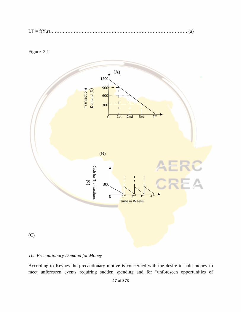
47 of 373

LT = f(Y,r)…………………………………………………………………………….(a)

Figure 2.1

(A)

(B)

(C)

The Precautionary Demand for Money

According to Keynes the precautionary motive is concerned with the desire to hold money to

meet unforeseen events requiring sudden spending and for “unforeseen opportunities of

0 1st 2nd 3rd 4th

300

600

900

1200

Tran

sact

ion

s

Dem

and

(¢

)

0 1st 2nd 3rd 4th

Time in Weeks

Cash

for Tran

saction

s

(¢) 300

48 of 373

advantageous purchases.” Both individuals and businessmen keep money to meet unexpected

needs. For example, individuals hold some money to provide for illness, accidents, and

unexpected visits from relatives, unemployment and other unforeseen contingencies. In the

same vein, businessmen reserve cash take advantages of gains from unexpected deals or to

overcome unfavourable conditions.

The precautionary demand for money depends upon the level of income, and business activity,

opportunities for unexpected profitable deals, availability of cash, the cost of holding liquid

assets in bank reserves, etc. Keynes believed that the precautionary demand for money, like

transactions demand, was a function of the level of income. But the post-Keynesian economists

believe that like transactions demand, it is inversely a function of income and interest rate. Thus

precautionary demand has the same determinants as the transactions demand. The demand for

money for these two purposes can therefore be represented by a single equation LT = f(Y,r)”.

The Speculative Demand for Money

Keynes believed that wealth could be held in a form of money which does not earn any rate of

return and in the form of bonds which do. So then after keeping enough money balances for

transactions and precautionary purposes, of what value will the excess money be? Keynes argued

that such extra funds will be used in making speculative gains by investing in financial

instruments like bonds. Specifically, speculative (or asset or liquidity preference) demand

according to Keynes is desire to hold money for “securing profit from knowing better than the

market what the future will bring forth.” It arises because of uncertainty surrounding future

interest rate and is based on regressive expectation. Money held for speculative purposes is a

liquid store of value which can be invested at an opportune moment in interest-bearing bonds or

securities.

A bond holder has expected returns on the bond from two sources, namely, the bond yield, that

is, the interest payment he receives – and a potential capital gain/loss-an increase/decrease in the

price of the bond from the time he buys it and the time it is sold. The bond’s yield Y is usually

stated as the face value of the bond. The market rate of return on the bond r is the ratio of the

yield to the price of the bond Pb .For example, if a hundred-cedi bond has a yield of ₵5, the

percentage yield is 5%. If the price of the bond rises to ₵125, the ₵5 yield corresponds to a

market rate of 4 %, that is ₵5 ₵125⁄ . Thus the market rate is given as:

49 of 373

𝑟 =𝑌

𝑃𝑏 (1)

.(You remember bond prices and the rate of interest are inversely related to each other? Such that

the lower the bond prices the higher the interest rates, and vice versa?)

But the yield is a fixed amount stated as a percentage of the bond’s face value, so then the

market price of the bond is represented as:

𝑃𝑏 =𝑌

𝑟 (2)

The expected percentage capital gain g is the percentage increase in price from the purchase

price Pb. to the expected sale price 𝑃𝑏𝑒 . Thus the expression of for the percentage capital gain is

𝑔 = (𝑃𝑏𝑒 − 𝑃𝑏 Pb.⁄ From equations (1) and (2), with a fixed Y on the bond, an expected price 𝑃𝑏

𝑒

corresponds to an expected interest rate, 𝑟 = 𝑌 𝑃𝑏𝑒 ⁄ . Thus in terms of expected and current

interest rates, the capital gain can be written

as: 𝑔 =𝑌

𝑟𝑒−𝑌

𝑟𝑌

𝑟

(3)

Cancelling the Y terms and multiplying both the numerator and denominator by r gives:

𝑔 =𝑟

𝑟𝑒 − 1 (4)

Equation 6 represents the expected capital gains in terms of current and expected interest rates.

For example, if the current rate of interest is 5% and the buyer of the bond expects the rate to

decline to 4%, his expected capital gain would be:

𝑔 =0.05

𝑟𝑒0.04− 1 = 1.25 − 1 = 0.25 %

The total percentage return on a bond, that is total earnings e, will be the sum of the market rate

of interest at the time of the purchase and the capital gains. That is 𝑒 = 𝑟 + 𝑔. By substituting

for g from equation (4), the expression for the total percentage return will be presented as:

𝑒 = 𝑟 +𝑟

𝑟𝑒− 1 (5)

Individuals demand for money

Given the expected return on bonds as 𝑒, and with a zero return on holding cash, the asset

holding will be expected to buy more bonds if he expects the return 𝑒 to be greater than zero. If

the return on bonds is expected to be less than zero, the asset holder will put his liquid wealth in

money.

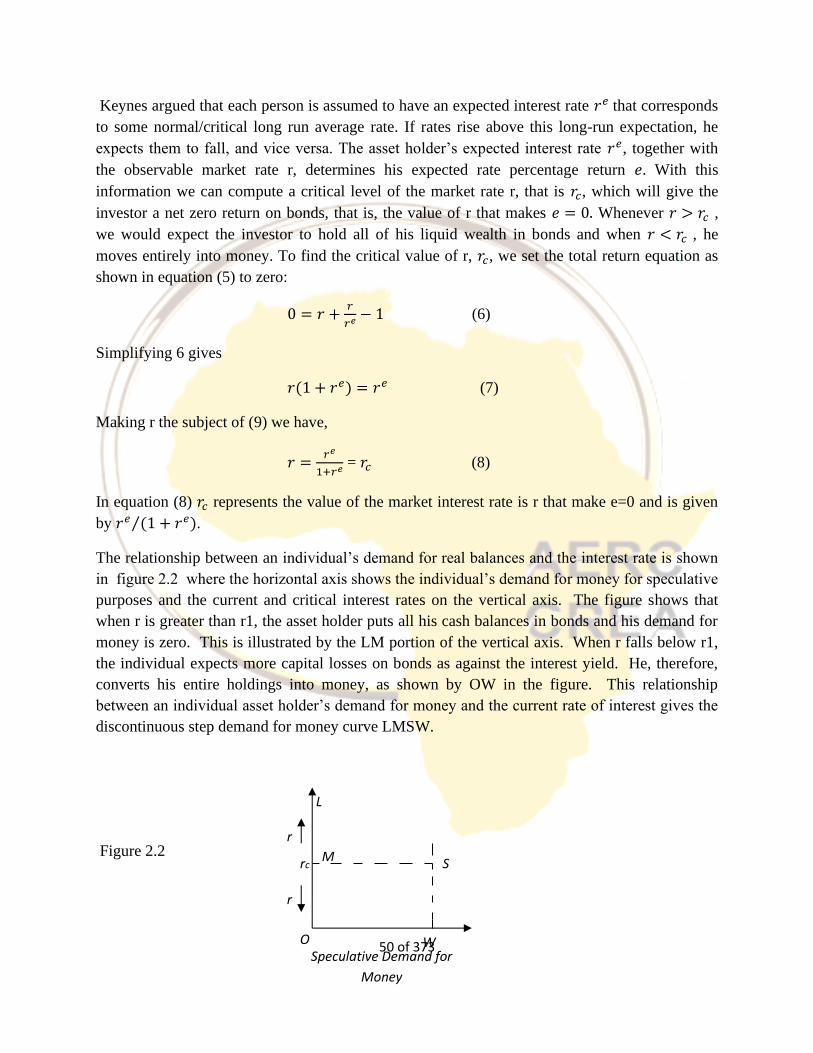
50 of 373

Keynes argued that each person is assumed to have an expected interest rate 𝑟𝑒 that corresponds

to some normal/critical long run average rate. If rates rise above this long-run expectation, he

expects them to fall, and vice versa. The asset holder’s expected interest rate 𝑟𝑒, together with

the observable market rate r, determines his expected rate percentage return 𝑒. With this

information we can compute a critical level of the market rate r, that is 𝑟𝑐, which will give the

investor a net zero return on bonds, that is, the value of r that makes 𝑒 = 0. Whenever 𝑟 > 𝑟𝑐 ,

we would expect the investor to hold all of his liquid wealth in bonds and when 𝑟 < 𝑟𝑐 , he

moves entirely into money. To find the critical value of r, 𝑟𝑐, we set the total return equation as

shown in equation (5) to zero:

0 = 𝑟 +𝑟

𝑟𝑒 − 1 (6)

Simplifying 6 gives

𝑟(1 + 𝑟𝑒) = 𝑟𝑒 (7)

Making r the subject of (9) we have,

𝑟 =𝑟𝑒

1+𝑟𝑒 = 𝑟𝑐 (8)

In equation (8) 𝑟𝑐 represents the value of the market interest rate is r that make e=0 and is given

by 𝑟𝑒 (1 + 𝑟𝑒⁄ ).

The relationship between an individual’s demand for real balances and the interest rate is shown

in figure 2.2 where the horizontal axis shows the individual’s demand for money for speculative

purposes and the current and critical interest rates on the vertical axis. The figure shows that

when r is greater than r1, the asset holder puts all his cash balances in bonds and his demand for

money is zero. This is illustrated by the LM portion of the vertical axis. When r falls below r1,

the individual expects more capital losses on bonds as against the interest yield. He, therefore,

converts his entire holdings into money, as shown by OW in the figure. This relationship

between an individual asset holder’s demand for money and the current rate of interest gives the

discontinuous step demand for money curve LMSW.

Figure 2.2

M S

W O

r

rc

r

L

Speculative Demand for

Money

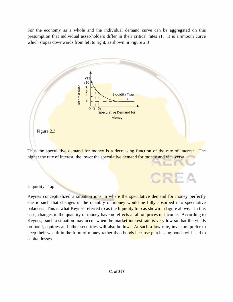
51 of 373

For the economy as a whole and the individual demand curve can be aggregated on this

presumption that individual asset-holders differ in their critical rates r1. It is a smooth curve

which slopes downwards from left to right, as shown in Figure 2.3

Figure 2.3

Thus the speculative demand for money is a decreasing function of the rate of interest. The

higher the rate of interest, the lower the speculative demand for money and vice versa.

Liquidity Trap

Keynes conceptualized a situation ions in where the speculative demand for money perfectly

elastic such that changes in the quantity of money would be fully absorbed into speculative

balances. This is what Keynes referred to as the liquidity trap as shown in figure above. In this

case, changes in the quantity of money have no effects at all on prices or income. According to

Keynes, such a situation may occur when the market interest rate is very low so that the yields

on bond, equities and other securities will also be low. At such a low rate, investors prefer to

keep their wealth in the form of money rather than bonds because purchasing bonds will lead to

capital losses.

2 4 6 8

r10 r12

0 S S1

Speculative Demand for

Money

Liquidity Trap

Inte

rest

Rat

e

52 of 373

The Total Demand for Money

We have considered the three motives for holding money according to the Keynesian system. By

putting these three together derive the total demand for money function. The transactions and

precautionary motives were seen to vary positive with the level of income and negatively with

the interest rate. The speculative demand for money was negatively related to the rate of

interest. Thus the total demand for money is a function of both income and the interest rate

which be presented as:

Md = f(Y,r)

Where Md represents the total demand for money, Y, income and r is the interest rate. A rise in

income increases money demand; a rise in the interest rate leads to a fall in money demand. The

money demand function can be represented in a linear form as:

𝑀𝑑=𝑐0 + 𝐶1𝑌 − 𝐶2𝑟 𝐶1 > 0, 𝐶2 < 0

Thus the total demand for money can be derived by the lateral summation of the demand

function for transactions and precautionary purposes and the demand function for speculative

purposes.

Criticisms of Keynes’ Theory:

James Tobin found two main weaknesses of the Keynesian theory of the speculative demand for

money:

(i) All-or-nothing choice:

In Keynes’ theory investors are assumed to hold all their wealth in bonds (other than the amount

of money held for transaction purposes) as long as the rate of interest exceeded the ‘critical rate’

— a rate below which the expected capital loss on bonds outweighed the interest earnings on

bonds. If, on the contrary, the interest rate fell below the critical level, investors would hold no

bonds, i.e., they would hold their entire wealth in money. So Keynes’ theory cannot explain why

and how an individual investor diversifies his portfolio by holding both money and bonds as

stores of wealth.

(ii) Changes in the normal rate of interest:

53 of 373

Keynes assumed that investors hold money as an asset so long as the interest rate is low. The

reason is that they expect the interest rate to rise and return to ‘normal’ level. According to

Keynes there exists a fixed or a slowly changing normal level for the interest rate, around which

the actual rate of interest gravitates.

So the normal rate is taken as a benchmark against which to judge the possibility of interest rate

changes which determine the amount of money held for speculative purposes.

According to Tobin the normal level itself keeps on changing over time — as has been shown by

the experience of the 1950s. This explains why portfolio diversification takes place. An

individual’s portfolio choice, i.e., his decision to diversify does not depend on Keynes’

restrictive assumption about investor expectations of a return of the interest rate to a normal

level. It is against this backdrop that we study Tobin’s portfolio theory of demand for money.

In short, Keynes’ followers such as James Tobin have not been satisfied with his theory of

speculative demand for money which seeks to explain the inverse relationship between the

interest rate and money demand. They have identified other reasons for the dependence of

demand for money on the interest rate.

W. J. Baumol and Tobin have also extended Keynes’ analysis of the transactions demand for

money. We may now discuss these two extensions of Keynes’ theory one by one.

On the other hand non-Keynesians — called monetarists — have refined and modified the

classical quantity theory of money. This is another notable development in the area of monetary

economics. Friedman’s analysis treats the demand for money in the same way as the demand for

an ordinary commodity. It can be viewed as a producer’s good; businesses hold cash balances to

improve efficiency in their financial transactions and are willing to pay, in terms of forgone

interest income, for this efficiency. Money can also be viewed as a consumer’s good; it yields

utility to the consumer in terms of smoothing out timing differences between the expenditure and

income streams and also in terms of reducing risk.

1.2.2 Theories of Demand of Money: Baumol and Tobin-Markowitz Model

Introduction

In this lecture, we discuss the Post-Keynesian theories of demand for money put forward by

Tobin, Baumol and Friedman.

By introducing speculative demand for money, Keynes made a significant departure from the

classical theory of money demand which emphasized only the transactions demand for money.

54 of 373

However, as seen above, Keynes’ theory of speculative demand for money has been challenged.

The main drawback of Keynes’ speculative demand for money is that it visualises that people

hold their assets in either all money or all bonds. This seems quite unrealistic as individuals hold

their financial wealth in some combination of both money and bonds.

This gave rise to portfolio approach to demand for money put forward by Tobin, Baumol and

Freidman. The portfolio of wealth consists of money, interest-bearing bonds, shares, physical

assets etc. Further, while according to Keynes’ theory, demand for money for transaction

purposes is insensitive to interest rate, the modem theories of money demand put forward by

Baumol and Tobin show that money held for transaction purposes is interest elastic.

1. Tobin’s Portfolio Approach to Demand for Money

An American economist James Tobin, in his important contribution explained that rational

behaviour on the part of the individuals is that they should keep a portfolio of assets which

consists of both bonds and money. In his analysis he makes a valid assumption that people prefer

more wealth to less.

According to him, an investor is faced with a problem of what proportion of his portfolio of

financial assets he should keep in the form of money (which earns no interest) and interest-

bearing bonds. The portfolio of individuals may also consist of more risky assets such as shares.

According to Tobin, faced with various safe and risky assets, individuals diversify their portfolio

by holding a balanced combination of safe and risky assets.

According to Tobin, individual’s behaviour shows risk aversion. That is, they prefer less risk to

more risk at a given rate of return. In the Keynes’ analysis an individual holds his wealth in

either all money or all bonds depending upon his estimate of the future rate of interest.

But, according to Tobin, individuals are uncertain about future rate of interest. If a wealth holder

chooses to hold a greater proportion of risky assets such as bonds in his portfolio, he will be

earning a high average return but will bear a higher degree of risk. Tobin argues that a risk

averter will not opt for such a portfolio with all risky bonds or a greater proportion of them.

On the other hand, a person who, in his portfolio of wealth, holds only safe and riskless assets

such as money (in the form of currency and demand deposits in banks) he will be taking almost

zero risk but will also be having no return and as a result there will be no growth of his wealth.

Therefore, people generally prefer a mixed diversified portfolio of money, bonds and shares,

with each person opting for a little different balance between riskiness and return.

It is important to note that a person will be unwilling to hold all risky assets such as bonds unless

he obtains a higher average return on them. In view of the desire of individuals to have both

safety and reasonable return, they strike a balance between them and hold a mixed and balanced

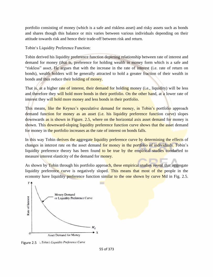
55 of 373

portfolio consisting of money (which is a safe and riskless asset) and risky assets such as bonds

and shares though this balance or mix varies between various individuals depending on their

attitude towards risk and hence their trade-off between risk and return.

Tobin‘s Liquidity Preference Function:

Tobin derived his liquidity preference function depicting relationship between rate of interest and

demand for money (that is, preference for holding wealth in money form which is a safe and

“riskless” asset. He argues that with the increase in the rate of interest (i.e. rate of return on

bonds), wealth holders will be generally attracted to hold a greater fraction of their wealth in

bonds and thus reduce their holding of money.

That is, at a higher rate of interest, their demand for holding money (i.e., liquidity) will be less

and therefore they will hold more bonds in their portfolio. On the other hand, at a lower rate of

interest they will hold more money and less bonds in their portfolio.

This means, like the Keynes’s speculative demand for money, in Tobin’s portfolio approach

demand function for money as an asset (i.e. his liquidity preference function curve) slopes

downwards as is shown in Figure. 2.5, where on the horizontal axis asset demand for money is

shown. This downward-sloping liquidity preference function curve shows that the asset demand

for money in the portfolio increases as the rate of interest on bonds falls.

In this way Tobin derives the aggregate liquidity preference curve by determining the effects of

changes in interest rate on the asset demand for money in the portfolio of individuals. Tobin’s

liquidity preference theory has been found to be true by the empirical studies conducted to

measure interest elasticity of the demand for money.

As shown by Tobin through his portfolio approach, these empirical studies reveal that aggregate

liquidity preference curve is negatively sloped. This means that most of the people in the

economy have liquidity preference function similar to the one shown by curve Md in Fig. 2.5.

Figure 2.5

56 of 373

Tobin’s approach has done away with the limitation of Keynes’ theory of liquidity preference for

speculative motive, namely, individuals hold their wealth in either all money or all bonds. Thus,

Tobin’s approach, according to which individuals simultaneously hold both money and bonds

but in different proportion at different rates of interest yields a continuous liquidity preference

curve.

Further, Tobin’s analysis of simultaneous holding of money and bonds is not based on the

erroneous Keynes’s assumption that interest rate will move only in one direction but on a simple

fact that individuals do not know with certainty which way the interest rate will change.

It is worth mentioning that Tobin’s portfolio approach, according to which liquidity preference

(i.e. demand for money) is determined by the individual’s attitude towards risk, can be extended

to the problem of asset choice when there are several alternative assets, not just two, of money

and bonds.

2. Baumol’s Inventory Approach to Transactions Demand for Money:

Instead of Keynes’s speculative demand for money, Baumol concentrated on transactions

demand for money and put forward a new approach to explain it. Baumol explains the

transaction demand for money from the viewpoint of the inventory control or inventory

management similar to the inventory management of goods and materials by business firms.

As businessmen keep inventories of goods and materials to facilitate transactions or exchange in

the context of changes in demand for them, Baumol asserts that individuals also hold inventory

of money because this facilitates transactions (i.e. purchases) of goods and services.

In view of the cost incurred on holding inventories of goods there is need for keeping optimal

inventory of goods to reduce cost. Similarly, individuals have to keep optimum inventory of

money for transaction purposes. Individuals also incur cost when they hold inventories of money

for transactions purposes.

They incur cost on these inventories as they have to forgone interest which they could have

earned if they had kept their wealth in saving deposits or fixed deposits or invested in bonds.

This interest income forgone is the cost of holding money for transactions purposes. In this way

Baumol and Tobin emphasised that transaction demand for money is not independent of the rate

of interest.

It may be noted that by money we mean currency and demand deposits which are quite safe and

riskless but carry no interest. On the other hand, bonds yield interest or return but are risky and

may involve capital loss if wealth holders invest in them.

However, saving deposits in banks, according to Baumol, are quite free from risk and also yield

some interest. Therefore, Baumol asks the question why an individual holds money (i.e. currency

57 of 373

and demand deposits) instead of keeping his wealth in saving deposits which are quite safe and

earn some interest as well.

According to him, it is for convenience and capability of it being easily used for transactions of

goods that people hold money with them in preference to the saving deposits. Unlike Keynes

both Baumol and Tobin argue that transactions demand for money depends on the rate of

interest.

People hold money for transaction purposes “to bridge the gap between the receipt of income

and its spending.” As interest rate on saving deposits goes up people will tend to shift a part of

their money holdings to the interest-bearing saving deposits.

Individuals compare the costs and benefits of funds in the form of money with the interest-

bearing saving deposits. According to Baumol, the cost which people incur when they hold funds

in money is the opportunity cost of these funds, that is, interest income forgone by not putting

them in saving deposits.

Tobin’s Portfolio Balance Approach (With Diagram) | Demand for Money

Let us make an in-depth study of the Tobin’s Portfolio Balance Approach.

The main problem with Keynesian approach to the demand for money is that it suggests that

individuals should, at any given time, hold all their liquid assets either in money or in bonds, but

not some of each. This is obviously not true in reality. The second approach — Tobin’s model of

liquidity preference — deals with this problem by showing that if the return on bonds is

uncertain, that is, bonds are risky, then the investor worrying about both risk and return is likely

to do best by holding both bonds and money.

Portfolio theories like the one presented by Tobin emphasises the role of money as a store of

value. According to these theories, people hold money as part of their portfolio of assets. The

reason for this is that money offers a different combination of risk and return than other assets

which are less liquid than money — such as bonds. To be more specific, money offers a safe

(nominal) return, whereas the prices of stocks and bonds may rise or fall. Thus Tobin has

suggested that households choose to hold money as part of their optimal portfolio.

Portfolio theories predict that the demand for money depends on the risk and return associated

with money holding as also on various other assets households can hold instead

of money. Furthermore, the demand for money should depend on real wealth, because wealth

measures the size of the portfolio to be allocated among money and the alternative assets.

For instance, the money demand function may be expressed as:

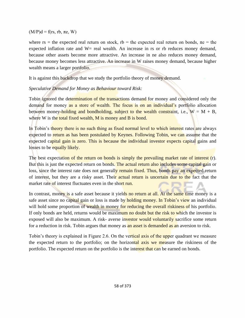
58 of 373

(M/P)d = f(rs, rb, πe, W)

where rs = the expected real return on stock, rb = the expected real return on bonds, πe = the

expected inflation rate and W= real wealth. An increase in rs or rb reduces money demand,

because other assets become more attractive. An increase in ne also reduces money demand,

because money becomes less attractive. An increase in W raises money demand, because higher

wealth means a larger portfolio.

It is against this backdrop that we study the portfolio theory of money demand.

Speculative Demand for Money as Behaviour toward Risk:

Tobin ignored the determination of the transactions demand for money and considered only the

demand for money as a store of wealth. The focus is on an individual’s portfolio allocation

between money-holding and bondholding, subject to the wealth constraint, i.e., W = M + B,

where W is the total fixed wealth, M is money and B is bond.

In Tobin’s theory there is no such thing as fixed normal level to which interest rates are always

expected to return as has been postulated by Keynes. Following Tobin, we can assume that the

expected capital gain is zero. This is because the individual investor expects capital gains and

losses to be equally likely.

The best expectation of the return on bonds is simply the prevailing market rate of interest (r).

But this is just the expected return on bonds. The actual return also includes some capital gain or

loss, since the interest rate does not generally remain fixed. Thus, bonds pay an expected return

of interest, but they are a risky asset. Their actual return is uncertain due to the fact that the

market rate of interest fluctuates even in the short run.

In contrast, money is a safe asset because it yields no return at all. At the same time money is a

safe asset since no capital gain or loss is made by holding money. In Tobin’s view an individual

will hold some proportion of wealth in money for reducing the overall riskiness of his portfolio.

If only bonds are held, returns would be maximum no doubt but the risk to which the investor is

exposed will also be maximum. A risk- averse investor would voluntarily sacrifice some return

for a reduction in risk. Tobin argues that money as an asset is demanded as an aversion to risk.

Tobin’s theory is explained in Figure 2.6. On the vertical axis of the upper quadrant we measure

the expected return to the portfolio; on the horizontal axis we measure the riskiness of the

portfolio. The expected return on the portfolio is the interest that can be earned on bonds.

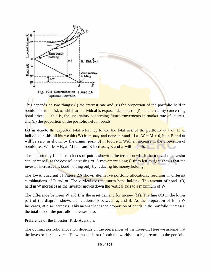
59 of 373

This depends on two things: (i) the interest rate and (ii) the proportion of the portfolio held in

bonds. The total risk to which an individual is exposed depends on (i) the uncertainty concerning

bond prices — that is, the uncertainty concerning future movements in market rate of interest,

and (ii) the proportion of the portfolio held in bonds.

Let us denote the expected total return by R and the total risk of the portfolio as a σt. If an

individual holds all his wealth (W) in money and none in bonds, i.e., W = M + 0, both R and σt

will be zero, as shown by the origin (point 0) in Figure 1. With an increase in the proportion of

bonds, i.e., W = M + B; as M falls and B increases, R and a, will both rise.

The opportunity line C is a locus of points showing the terms on which the individual investor

can increase R at the cost of increasing σt. A movement along C from left to right shows that the

investor increases his bond holding only by reducing his money holding.

The lower quadrant of Figure 2.6 shows alternative portfolio allocations, resulting in different

combinations of R and σt. The vertical axis measures bond holding. The amount of bonds (B)

held in W increases as the investor moves down the vertical axis to a maximum of W.

The difference between W and B is the asset demand for money (M). The line OB in the lower

part of the diagram shows the relationship between a, and B. As the proportion of B in W

increases, σt also increases. This means that as the proportion of bonds in the portfolio increases,

the total risk of the portfolio increases, too.

Preference of the Investor: Risk-Aversion:

The optimal portfolio allocation depends on the preferences of the investor. Here we assume that

the investor is risk-averse. He wants the best of both the worlds — a high return on the portfolio

Figure 2.6

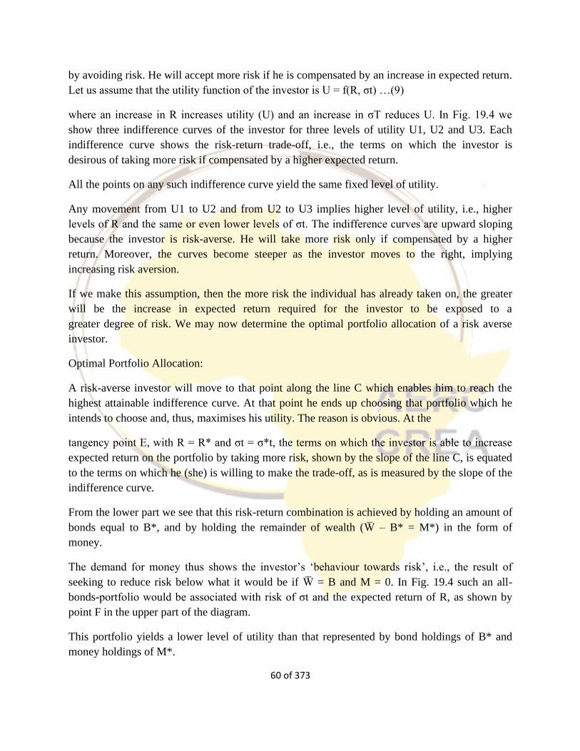
60 of 373

by avoiding risk. He will accept more risk if he is compensated by an increase in expected return.

Let us assume that the utility function of the investor is U = f(R, σt) …(9)

where an increase in R increases utility (U) and an increase in σT reduces U. In Fig. 19.4 we

show three indifference curves of the investor for three levels of utility U1, U2 and U3. Each

indifference curve shows the risk-return trade-off, i.e., the terms on which the investor is

desirous of taking more risk if compensated by a higher expected return.

All the points on any such indifference curve yield the same fixed level of utility.

Any movement from U1 to U2 and from U2 to U3 implies higher level of utility, i.e., higher

levels of R and the same or even lower levels of σt. The indifference curves are upward sloping

because the investor is risk-averse. He will take more risk only if compensated by a higher

return. Moreover, the curves become steeper as the investor moves to the right, implying

increasing risk aversion.

If we make this assumption, then the more risk the individual has already taken on, the greater

will be the increase in expected return required for the investor to be exposed to a

greater degree of risk. We may now determine the optimal portfolio allocation of a risk averse

investor.

Optimal Portfolio Allocation:

A risk-averse investor will move to that point along the line C which enables him to reach the

highest attainable indifference curve. At that point he ends up choosing that portfolio which he

intends to choose and, thus, maximises his utility. The reason is obvious. At the

tangency point E, with R = R* and σt = σ*t, the terms on which the investor is able to increase

expected return on the portfolio by taking more risk, shown by the slope of the line C, is equated

to the terms on which he (she) is willing to make the trade-off, as is measured by the slope of the

indifference curve.

From the lower part we see that this risk-return combination is achieved by holding an amount of

bonds equal to B*, and by holding the remainder of wealth (W̅ – B* = M*) in the form of

money.

The demand for money thus shows the investor’s ‘behaviour towards risk’, i.e., the result of

seeking to reduce risk below what it would be if W̅ = B and M = 0. In Fig. 19.4 such an all-

bonds-portfolio would be associated with risk of σt and the expected return of R, as shown by

point F in the upper part of the diagram.

This portfolio yields a lower level of utility than that represented by bond holdings of B* and

money holdings of M*.

61 of 373

The reason is that as the investor moves to the right of point E along the line 0C, the additional

return expected from the portfolio by holding more bonds (and less money) is not adequate to

compensate the investor for the additional risk (the slope of the line 0C is less than that of the

indifference curve U2). The movement to point F takes the investor to a lower indifference

curve, U1.

Interest Rate Changes and the Speculative Demand for Money:

In Tobin’s theory the amount of money held as an asset depends on the level of the interest rate.

Figure 2 shows the relationship between interest rate and asset demand for money. An increase

in the rate of interest from r0 to r1 and then to r2 will improve the terms on which the expected

return on the portfolio can be increased by taking more risk.

So the line 0C becomes steeper. It rotates anticlockwise from C(r0) to C(r1) and then to C(r2).

The investor responds by taking more risk and earning higher expected returns by moving from

E to F and then to G. It may be noted that each point is one of portfolio optimisation. In this case

his holdings of bonds (risky asset) increase (from B0 to B1, and then to B2) and money holdings

fall (from M0 to M1, then M2).

In short, as the interest rate rises, a given increase in risk, which corresponds to a given increase

in the amount of bonds in the portfolio, will result in a greater increase in expected return on the

portfolio. The box below presents a formal derivation of Tobin’s mean-variance model of bond

demand.

Box: Formal Derivation of Tobin’s mean-variance model of bond demand

Figure 2.7

62 of 373

Tobin looks at the choice between holding money, which earns a certain return of

zero, versus holding bonds, whose return can be stated as:

RB = i + g

where i = interest rate on the bond; g = capital gain

Tobin also assumes that the expected capital gain is zero5 and that its variance is 𝛿𝑔2

E(g) = 0 and so E(RB) = i + 0 = i

Var(g) = E[g - E(g)]2 = E(g2) = 𝛿𝑔2

where E = expectation of the variable inside the parentheses

Var = variance of the variable inside the parentheses

If A is the fraction of the portfolio put into bonds (0≤A≥1) and 1 - A is the fraction of the portfolio

held as money, the return R on the portfolio can be written as:

R = ARB + (1 - A)(0) = ARB = A(i + g)

Then the mean and variance of the return on the portfolio, denoted respectively by 𝜇

and 𝛿2 can be calculated as follows:

𝜇 = E(R) = E(ARB) = AE(RB) = Ai

𝛿2 = E(R - 𝜇)2 = E[A(i + g) – Ai]2 = E(Ag)2 = A2E(g2) = A2𝛿𝑔2

Taking the square root of both sides of the equation directly above and solving for A

yields: 𝐴 =1

𝜎𝑔𝜎 (2)

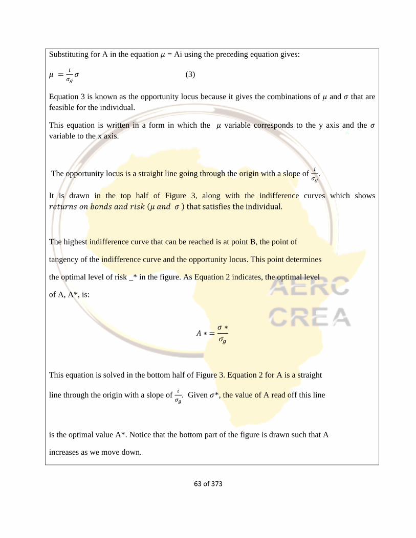
63 of 373

Substituting for A in the equation 𝜇 = Ai using the preceding equation gives:

𝜇 =𝑖

𝜎𝑔𝜎 (3)

Equation 3 is known as the opportunity locus because it gives the combinations of 𝜇 and 𝜎 that are

feasible for the individual.

This equation is written in a form in which the 𝜇 variable corresponds to the y axis and the 𝜎

variable to the x axis.

The opportunity locus is a straight line going through the origin with a slope of 𝑖

𝜎𝑔.

It is drawn in the top half of Figure 3, along with the indifference curves which shows

𝑟𝑒𝑡𝑢𝑟𝑛𝑠 𝑜𝑛 𝑏𝑜𝑛𝑑𝑠 𝑎𝑛𝑑 𝑟𝑖𝑠𝑘 (𝜇 𝑎𝑛𝑑 𝜎 ) that satisfies the individual.

The highest indifference curve that can be reached is at point B, the point of

tangency of the indifference curve and the opportunity locus. This point determines

the optimal level of risk _* in the figure. As Equation 2 indicates, the optimal level

of A, A*, is:

𝐴 ∗ =𝜎 ∗

𝜎𝑔

This equation is solved in the bottom half of Figure 3. Equation 2 for A is a straight

line through the origin with a slope of 𝑖

𝜎𝑔. Given 𝜎*, the value of A read off this line

is the optimal value A*. Notice that the bottom part of the figure is drawn such that A

increases as we move down.

64 of 373

Now what happens when the interest rate falls from i2 to i1.

This situation is shown in the Figure below. Because 𝜎𝑔g is unchanged, the Equation 2 line in the

bottom half of the figure does not change. However, the slope of the opportunity locus

does decrease as i decreases.

Thus, the opportunity locus rotates down and we move from point C to point B at the tangency of

the new opportunity locus and the indifference curve.

As is shown it is shown in the graph. the optimal level of risk decreases from 𝜎21* to 𝜎1* , and the

optimal fraction of the portfolio held in bonds falls from A2 * to A1 * .

The result is that as the interest rate on bonds falls, the demand for money increase; that is, 1 - A,

the fraction of the portfolio held as money, increases.

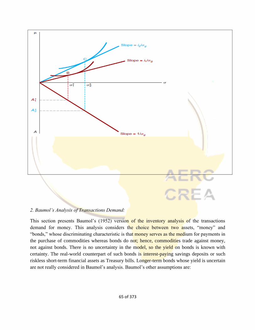
65 of 373

2. Baumol’s Analysis of Transactions Demand:

This section presents Baumol’s (1952) version of the inventory analysis of the transactions

demand for money. This analysis considers the choice between two assets, “money” and

“bonds,” whose discriminating characteristic is that money serves as the medium for payments in

the purchase of commodities whereas bonds do not; hence, commodities trade against money,

not against bonds. There is no uncertainty in the model, so the yield on bonds is known with

certainty. The real-world counterpart of such bonds is interest-paying savings deposits or such

riskless short-term financial assets as Treasury bills. Longer-term bonds whose yield is uncertain

are not really considered in Baumol’s analysis. Baumol’s other assumptions are:

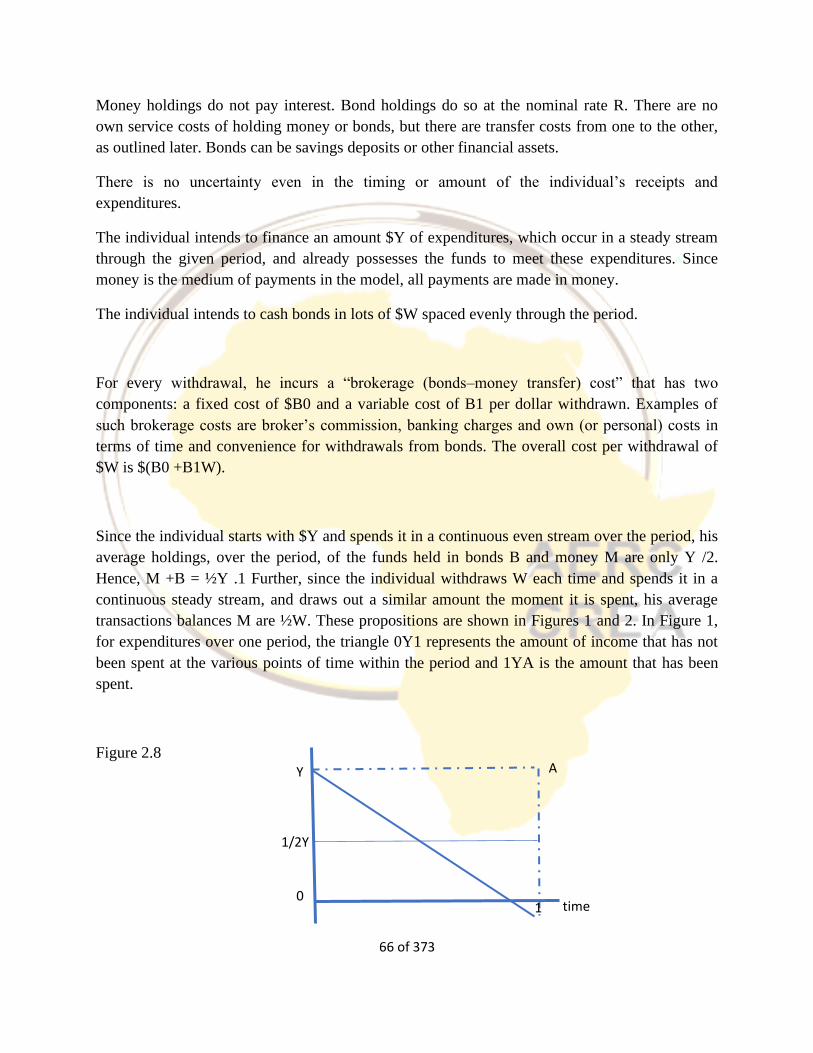
66 of 373

Money holdings do not pay interest. Bond holdings do so at the nominal rate R. There are no

own service costs of holding money or bonds, but there are transfer costs from one to the other,

as outlined later. Bonds can be savings deposits or other financial assets.

There is no uncertainty even in the timing or amount of the individual’s receipts and

expenditures.

The individual intends to finance an amount $Y of expenditures, which occur in a steady stream

through the given period, and already possesses the funds to meet these expenditures. Since

money is the medium of payments in the model, all payments are made in money.

The individual intends to cash bonds in lots of $W spaced evenly through the period.

For every withdrawal, he incurs a “brokerage (bonds–money transfer) cost” that has two

components: a fixed cost of $B0 and a variable cost of B1 per dollar withdrawn. Examples of

such brokerage costs are broker’s commission, banking charges and own (or personal) costs in

terms of time and convenience for withdrawals from bonds. The overall cost per withdrawal of

$W is $(B0 +B1W).

Since the individual starts with $Y and spends it in a continuous even stream over the period, his

average holdings, over the period, of the funds held in bonds B and money M are only Y /2.

Hence, M +B = ½Y .1 Further, since the individual withdraws W each time and spends it in a

continuous steady stream, and draws out a similar amount the moment it is spent, his average

transactions balances M are ½W. These propositions are shown in Figures 1 and 2. In Figure 1,

for expenditures over one period, the triangle 0Y1 represents the amount of income that has not

been spent at the various points of time within the period and 1YA is the amount that has been

spent.

Figure 2.8

A

1/2Y

Y

0 time 1

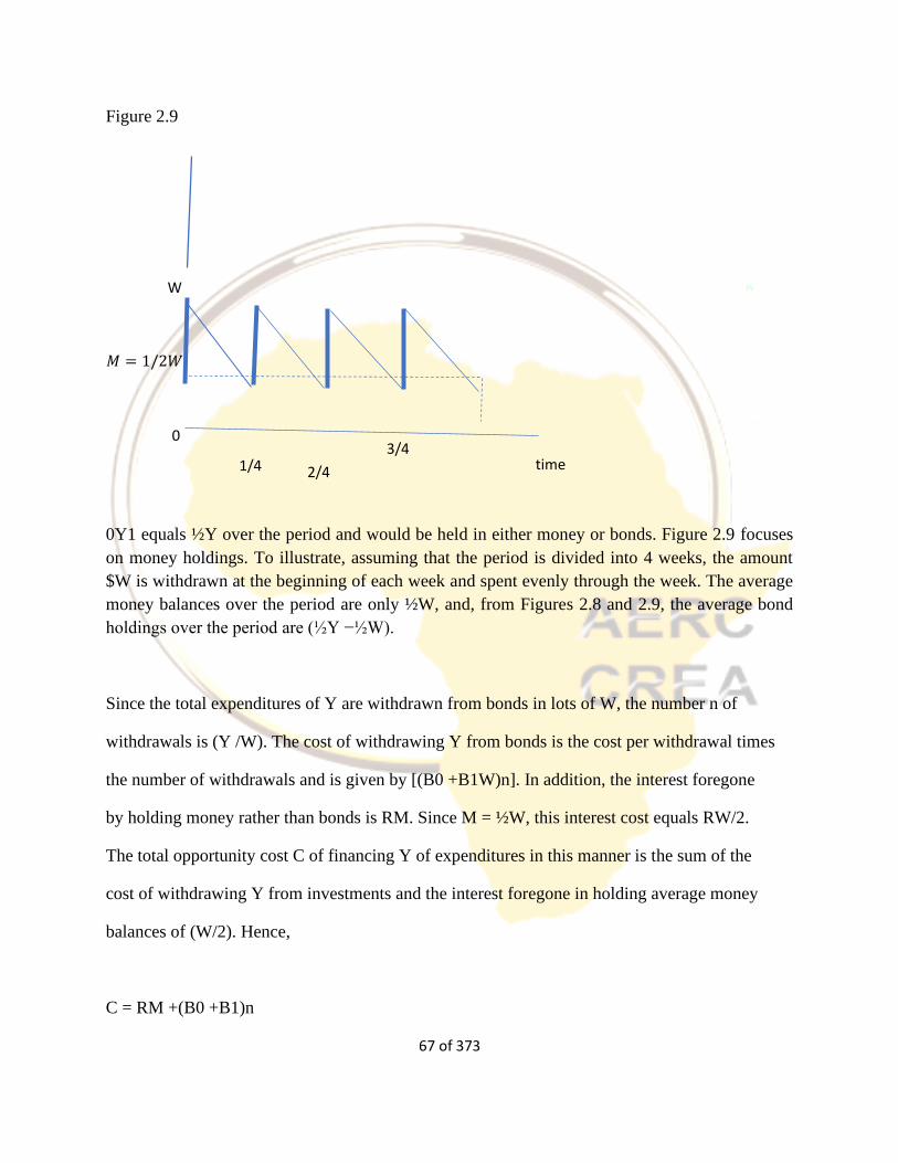
67 of 373

Figure 2.9

0Y1 equals ½Y over the period and would be held in either money or bonds. Figure 2.9 focuses

on money holdings. To illustrate, assuming that the period is divided into 4 weeks, the amount

$W is withdrawn at the beginning of each week and spent evenly through the week. The average

money balances over the period are only ½W, and, from Figures 2.8 and 2.9, the average bond

holdings over the period are (½Y −½W).

Since the total expenditures of Y are withdrawn from bonds in lots of W, the number n of

withdrawals is (Y /W). The cost of withdrawing Y from bonds is the cost per withdrawal times

the number of withdrawals and is given by [(B0 +B1W)n]. In addition, the interest foregone

by holding money rather than bonds is RM. Since M = ½W, this interest cost equals RW/2.

The total opportunity cost C of financing Y of expenditures in this manner is the sum of the

cost of withdrawing Y from investments and the interest foregone in holding average money

balances of (W/2). Hence,

C = RM +(B0 +B1)n

𝑀 = 1/2𝑊

W

time 3/4

1/4 2/4

0

68 of 373

= RW/2+B0 · Y /W +B1Y (1)

If the individual acts rationally in trying to meet his payments Y at minimum cost, he will

minimize the cost C of holding transactions balances. To do so, set the derivative of (1) with

respect to W equal to zero. This yields:

∂C/∂W = R/2−B0 · Y /W2 = 0 (2)

so that:

W = [2B0 · Y /R]½ (3)

and

Mtr = ½W = (½B0)½Y−½R−½ (4)

where we have inserted the superscript tr to emphasize that (4) specifies only the transactions

demand for money and does not include the money demand that would arise for speculative and

other motives. (4) is called the square root formula in inventory analysis and has the easily

identifiable form of a Cobb–Douglas function. In the present analysis, it specifies the

demand for transactions balances for a cost-minimizing individual. The preceding demand

function is clearly different from Keynes’s demand function for transactions balances and,

among other things, indicates that the demand for transactions balances depends upon the

nominal rate of interest. The properties of this demand function, showing its response to changes

in the real levels of expenditures, interest rates and prices, are discussed below. Brokerage costs

are the prices charged for brokerage services, which are commodities (i.e. “goods and services”),

so that:

let B0 = P.b0 and B1 = P.b1, where b0 and b1 are the elements of the brokerage charge in real

terms,

69 of 373

whereas B0 and B1 were nominal brokerage charges, and P is the price level. The reason for

expressing brokerage costs in this way is that the brokerage services related to money

withdrawals from earning assets are themselves commodities and, from a rigorous viewpoint, if

the prices of all commodities double, the brokerage cost must also double. Hence, both B0 and

B1 must be taken to increase in the same proportion as the commodity price level P.

Therefore, equation (4) can be rewritten as:

Mtr,d = (½b0)½Py½R−½ (5)

and

Mtr,d/P = mtr = (½b0)½y½R−½

Therefore, the elasticities of the transactions demand for money with respect to y, R and P, are:

Em.y = ½; Em.R =−½; EM.P = 1; Em.P = 0

The profitability of Holding Money and Bonds for Transactions

Based on the Baumol-Tobin model of the transaction demand for money, assume that a person

has income/expenditure $Y, Bond savings B which earns interest R, money holdings M and cash

bonds cash bonds in lots of $W spaced evenly through the period. If every withdrawal, he incurs

a “brokerage (bonds–money transfer) cost” that has two components: a fixed cost of $B0 and a

variable cost of B1 per dollar withdrawn, derive an expression for the optimal number of trips

(n*) that minimizes the total cost.

The average nominal holdings B of bonds are equal to (½Y −M), where, as before, M equals

½W. The individual earns interest at the rate R on these bond holdings.

The profit from holding either money or bonds equals this interest income from holding bonds

less the brokerage cost of money withdrawals from bonds.

That is, the profit π from using the combinations of money and bonds is given by:

π = interest income from bonds − brokerage expenses

= R · B−(B0 +B1W)n

70 of 373

= R {½Y −M } – {½B0Y /M +B1Y} ……………………………..(1)

Maximizing (1) with respect to M yields the first-order maximizing condition as:

∂π/∂M =−R+½B0Y /M2 = 0 ……………………………(2)

Hence, as in,

Mtr = (½B0)½Y ½R−½

Further,

Btr = ½Y −((½B0)½Y ½R−½)

where the superscript tr on B emphasizes that this demand for bonds is only for transactions

purposes. Hence, from (1),

π = R{½Y −((½B0)½Y ½R−½ }−{(½B0 )Y /[((½B0)½Y ½R−½]+B1Y}……………….(3)

= ½RY −((½B0)½Y ½R½ −{((½B0)½Y ½R½ }−B1Y

= ½RY −2(½B0)½Y ½R½ −B1Y

Simplifying, we get:

π = ½RY −2RM −B1Y

= (½R−B1)Y −2RM ……………………………………………………………………(4)

ii) Equation (4) derived from the profit function above implies the following:

- total interest income from holding money and bonds is reduced by the interest cost of holding

money and the variable cost of withdrawing Y from bonds. Further, since the second term on the

right-hand side is nonpositive, the first term implies that, no matter what the level of income, it

would not be profitable to hold bonds unless R > 2B1.

-In equation (4), π is non-positive if R = 0 or if the total brokerage charges exceed the income

from holding bonds. The latter would occur if the brokerage costs are relatively high. Note in this

regard that the brokerage costs include both the charges explicitly levied by financial institutions

and any other costs of conversion from bonds to money. The latter include the time and

inconvenience, etc. – sometimes referred to as the “shoe-leather costs”

71 of 373

1.2.3 Friedman's Restatement of the Quantity Theory of Money

A noted monetarist economist Friedman put forward demand for money function which plays an

important role in his restatement of the quantity theory of money and prices. Friedman believes

that money demand function is most important stable function of macroeconomics. He treats

money as one type of asset in which wealth holders can keep a part of their wealth. Business

firms view money as a capital good or a factor of production which they combine with the

services of other productive assets or labour to produce goods and services. Thus, according to

Friedman, individuals hold money for the services it provides to them. It may be noted that the

service rendered by money is that it serves as a general purchasing power so that it can be

conveniently used for buying goods and services.

His approach to demand for money does not consider any motives for holding money, nor does it

distinguishes between speculative and transactions demand for money. Friedman considers the

demand for money merely as an application of a general theory of demand for capital assets.

Like other capital assets, money also yields return and provides services. He analyses the various

factors that determine the demand for money and from this analysis derives demand for money

function. Note that the value of goods and services which money can buy represents the real

yield on money. Obviously, this real yield of money in terms of goods and services which it can

purchase will depend on the price level of goods and services.

Besides money, bonds are another type of asset in which people can hold their wealth. Bonds are

securities which yield a stream of interest income, fixed in nominal terms. Yield on bond is the

coupon rate of interest and also anticipated capital gain or loss due to expected changes in the

market rate of interest.

Equities or Shares are another form of asset in which wealth can be held. The yield from equity

is determined by the dividend rate, expected capital gain or loss and expected changes in the

price level. The fourth form in which people can hold their wealth is the stock of producer and

durable consumer commodities.

These commodities also yield a stream of income but in kind rather than in money. Thus, the

basic yield from commodities is implicit one. However, Friedman also considers an explicit yield

from commodities in the form of expected rate of change in their price per unit of time.

Friedman’s nominal demand function (Md) for money can be written as

Md=f (W, h, rm, rb, re, P, ∆P/P, U)

As demand for real money balances is nominal demand for money divided by the price level,

demand for real money balances can be written as

Md/P = f(W, h, rm, rb, re, P, ∆P/P, U)

72 of 373

Where Md stands for nominal demand for money and Md/P for demand for real money balances,

W stands for wealth of the individuals, h for the proportion of human wealth to the total wealth

held by the individuals, rm for rate of return or interest on money, rb for rate of interest on

bonds, re for rate of return on equities, P for the price level, ∆P/P for the change in price level

{i.e. rate of inflation), and U for the institutional factors.

1. Wealth (W):

The major factor determining the demand for money is the wealth of the individual (W) In

wealth Friedman includes not only non-human wealth such as bonds, shares, money which yield

various rates of return but also human wealth or human capital. By human wealth Friedman

means the value of an individual’s present and future earnings.

Whereas non-human wealth can be easily converted into money, that is, can be made liquid.

Such substitution of human wealth is not easily possible. Thus human wealth represents illiquid

component of wealth and, therefore, the proportion of human wealth to the non-human wealth

has been included in the demand for money function as an independent variable. Individual’s

demand for money directly depends on his total wealth. Indeed, the total wealth of an individual

represents an upper limit of holding money by an individual and is similar to the budget

constraint of the consumer in the theory of demand.

The greater the wealth of an individual, the more money he will demand for transactions and

other purposes. As a country, becomes richer, its demand for money for transaction and other

purposes will increase. Since as compared to non- human wealth, human wealth is much less

liquid, Friedman has argued that as the proportion of human wealth in the total wealth increases,

there will be a greater demand for money to make up for the illiquidity of human wealth.

2. Rates of Interest or Return (rm, rb, re):

Friedman considers three rates of interest, namely, rb, re and rm,which determine the demand for

money, rm is the own rate of interest on money. Note that money kept in the form of currency

and demand deposits does not earn any interest.

But money held as saving deposits and fixed deposits earns certain rates of interest and it is this

rate of interest which is designated by rm in the money demand function. Given the other rates of

interest or return, the higher the own rate of interest, the greater the demand for money.

In deciding how large a part of his wealth to hold in the form of money the individual will

compare the rate of interest on money with rates of interest (or return) on bonds and other assets.

As mentioned earlier, the opportunity cost of holding money is the interest or return given up by

not holding these other forms of assets.

73 of 373

As rates of return on bond (rb) and equities (re) rise, the opportunity cost of holding money will

increase which will reduce the demand for money holdings. Thus, the demand for money is

negatively related to the rate of interest (or return) on bonds, equities and other such non-money

assets.

3. Price Level (P):

Price level also determines the demand for money balances. A higher price level means people

will require a larger nominal money balances in order to do the same amount of transactions, that

is, to purchase the same amount of goods and services.

If income (Y) is used as proxy for wealth (W) which, as stated above, is the most important

determinant of demand for money, then nominal income is given by Y.P which becomes a

crucial determinant of demand for money.

Here Y stands for real income (i.e. in terms of goods and services) and P for price level. As the

price level goes up, the demand for money will rise and, on the other hand, if price level falls, the

demand for money will decline. As a matter of fact, people adjust the nominal money balances

(M) to achieve their desired level of real money balances (M/P).

4. The Expected Rate of Inflation (∆P/P):

If people expect a higher rate of inflation, they will reduce their demand for money holdings.

This is because inflation reduces the value of their money balances in terms of its power to

purchase goods and services.

If the rate of inflation exceeds the nominal rate of interest, there will be negative rate of return on

money. Therefore, when people expect a higher rate of inflation they will tend to convert their

money holdings into goods or other assets which are not affected by inflation.

On the other hand, if people expect a fall in the price level, their demand for money holdings will

increase.

5. Institutional Factors (U):

Institutional factors such as mode of wage payments and bill payments also affect the demand

for money. Several other factors which influence the overall economic environment affect the

demand for money. For example, if recession or war is anticipated, the demand for money

balances will increase.

Besides, instability in capital markets, which erodes the confidence of the people in making

profits from investment in bonds and equity shares will also raise the demand for money. Even

political instability in the country influences the demand for money. To account for these

institutional factors Friedman includes the variable U in his demand for money function.

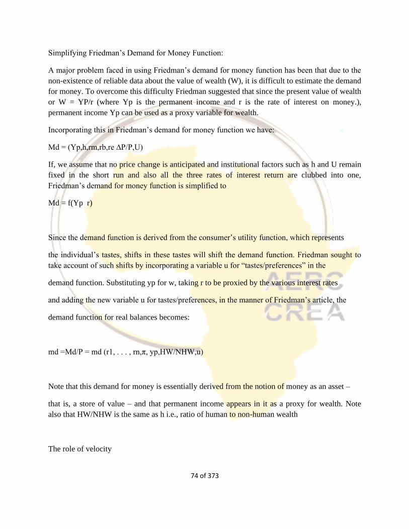
74 of 373

Simplifying Friedman’s Demand for Money Function:

A major problem faced in using Friedman’s demand for money function has been that due to the

non-existence of reliable data about the value of wealth (W), it is difficult to estimate the demand

for money. To overcome this difficulty Friedman suggested that since the present value of wealth

or W = YP/r (where Yp is the permanent income and r is the rate of interest on money.),

permanent income Yp can be used as a proxy variable for wealth.

Incorporating this in Friedman’s demand for money function we have:

Md = (Yp,h,rm,rb,re ∆P/P,U)

If, we assume that no price change is anticipated and institutional factors such as h and U remain

fixed in the short run and also all the three rates of interest return are clubbed into one,

Friedman’s demand for money function is simplified to

Md = f(Yp r)

Since the demand function is derived from the consumer’s utility function, which represents

the individual’s tastes, shifts in these tastes will shift the demand function. Friedman sought to

take account of such shifts by incorporating a variable u for “tastes/preferences” in the

demand function. Substituting yp for w, taking r to be proxied by the various interest rates

and adding the new variable u for tastes/preferences, in the manner of Friedman’s article, the

demand function for real balances becomes:

md =Md/P = md (r1, . . . , rn,π, yp,HW/NHW,u)

Note that this demand for money is essentially derived from the notion of money as an asset –

that is, a store of value – and that permanent income appears in it as a proxy for wealth. Note

also that HW/NHW is the same as h i.e., ratio of human to non-human wealth

The role of velocity

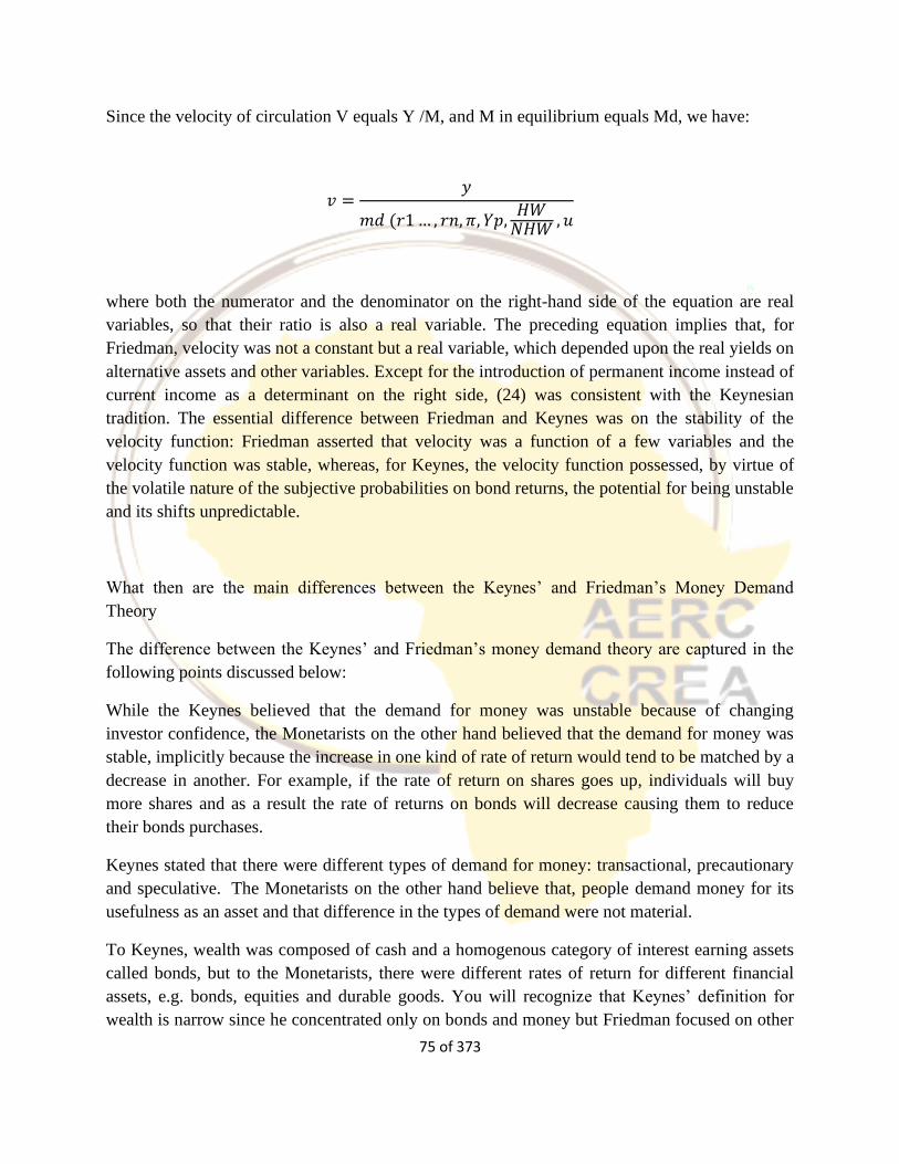
75 of 373

Since the velocity of circulation V equals Y /M, and M in equilibrium equals Md, we have:

𝑣 =𝑦

𝑚𝑑 (𝑟1 … , 𝑟𝑛, 𝜋, 𝑌𝑝,𝐻𝑊

𝑁𝐻𝑊 , 𝑢

where both the numerator and the denominator on the right-hand side of the equation are real

variables, so that their ratio is also a real variable. The preceding equation implies that, for

Friedman, velocity was not a constant but a real variable, which depended upon the real yields on

alternative assets and other variables. Except for the introduction of permanent income instead of

current income as a determinant on the right side, (24) was consistent with the Keynesian

tradition. The essential difference between Friedman and Keynes was on the stability of the

velocity function: Friedman asserted that velocity was a function of a few variables and the

velocity function was stable, whereas, for Keynes, the velocity function possessed, by virtue of

the volatile nature of the subjective probabilities on bond returns, the potential for being unstable

and its shifts unpredictable.

What then are the main differences between the Keynes’ and Friedman’s Money Demand

Theory

The difference between the Keynes’ and Friedman’s money demand theory are captured in the

following points discussed below:

While the Keynes believed that the demand for money was unstable because of changing

investor confidence, the Monetarists on the other hand believed that the demand for money was

stable, implicitly because the increase in one kind of rate of return would tend to be matched by a

decrease in another. For example, if the rate of return on shares goes up, individuals will buy

more shares and as a result the rate of returns on bonds will decrease causing them to reduce

their bonds purchases.

Keynes stated that there were different types of demand for money: transactional, precautionary

and speculative. The Monetarists on the other hand believe that, people demand money for its

usefulness as an asset and that difference in the types of demand were not material.

To Keynes, wealth was composed of cash and a homogenous category of interest earning assets

called bonds, but to the Monetarists, there were different rates of return for different financial

assets, e.g. bonds, equities and durable goods. You will recognize that Keynes’ definition for

wealth is narrow since he concentrated only on bonds and money but Friedman focused on other

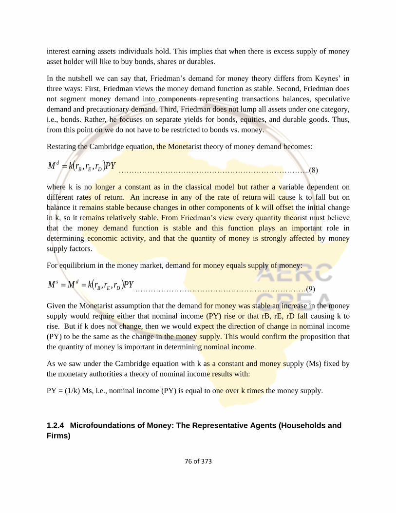
76 of 373

interest earning assets individuals hold. This implies that when there is excess supply of money

asset holder will like to buy bonds, shares or durables.

In the nutshell we can say that, Friedman’s demand for money theory differs from Keynes’ in

three ways: First, Friedman views the money demand function as stable. Second, Friedman does

not segment money demand into components representing transactions balances, speculative

demand and precautionary demand. Third, Friedman does not lump all assets under one category,

i.e., bonds. Rather, he focuses on separate yields for bonds, equities, and durable goods. Thus,

from this point on we do not have to be restricted to bonds vs. money.

Restating the Cambridge equation, the Monetarist theory of money demand becomes:

( )PYrrrkM DEB

d ,,= ………………………………………………………………..(8)

where k is no longer a constant as in the classical model but rather a variable dependent on

different rates of return. An increase in any of the rate of return will cause k to fall but on

balance it remains stable because changes in other components of k will offset the initial change

in k, so it remains relatively stable. From Friedman’s view every quantity theorist must believe

that the money demand function is stable and this function plays an important role in

determining economic activity, and that the quantity of money is strongly affected by money

supply factors.

For equilibrium in the money market, demand for money equals supply of money:

( )PYrrrkMM DEB

ds ,,==…………………………………………………………(9)

Given the Monetarist assumption that the demand for money was stable an increase in the money

supply would require either that nominal income (PY) rise or that rB, rE, rD fall causing k to

rise. But if k does not change, then we would expect the direction of change in nominal income

(PY) to be the same as the change in the money supply. This would confirm the proposition that

the quantity of money is important in determining nominal income.

As we saw under the Cambridge equation with k as a constant and money supply (Ms) fixed by

the monetary authorities a theory of nominal income results with:

PY = (1/k) Ms, i.e., nominal income (PY) is equal to one over k times the money supply.

1.2.4 Microfoundations of Money: The Representative Agents (Households and

Firms)

77 of 373

Introduction

In this section we will look at microfoundations of money and ways of introducing money into a

neoclassical model and how these methods can be developed in an effort to try and explain

certain facts. As in previous lectures, we shall find that while we can develop models to improve

our understanding of the business cycle we still remain some distance from a reliable model.

While we introduce money in ways which break the neoclassical dichotomy, the models we look

at are still partly neoclassical in nature.

The first problem with any neoclassical general equilibrium approach to business cycles when it

comes to modelling monetary phenomena is how to explain why consumers need to hold money.

Without a justification of why there is a demand for money it is obviously impossible to model

the impact that variations in money supply will have on the economy. There are three broad

approaches:

Money in the Utility Function - if utility depends upon real money balances then money is like

any other good and will be demanded by consumers. However, most people are reluctant to start

with this assumption as it is rather ad hoc. It is a far better modelling strategy to try and point to a

reason why money is held by consumers other than it is a direct source of utility. However, that

said it is well known that under certain conditions there exists an equivalence between putting

money in the utility function or specifying a transactions technology which involves money.

Cash in Advance Models - this is the route which has been most thoroughly explored in the

literature the assumption here is that before a consumer can buy goods they must pay for them in

cash. Therefore money is demanded because it is the only means of purchasing some goods

Transactions Cost (Shopping Time Technology) - in these models consumers have a choice

(unlike in

They can obtain goods on credit or barter or they can purchase goods with cash. However,

purchasing goods consumes resources and the more cash that an individual holds the lower these

shopping costs are (e.g. they can avoid very costly bartering processes). By holding money,

consumers lose any interest they would otherwise have gained on their savings but they

economise on their transactions costs.

In this lecture, I review the recent development of a microfoundations of money. To explain

what a microfoundations of money about and why it is necessary, let me list the main issues in

monetary economics as follows. (I) Existence and essentiality of fiat money. (II) Why would

intrinsically worthless money have value? (III) Is money a good or not?

78 of 373

In economics, the microfoundations are the microeconomic behavior of individual agents, such

as households or firms, that underpins an economic theory. Most early macroeconomic models,

including early Keynesian models, were based on hypotheses about relationships between

aggregate quantities, such as aggregate output, employment, consumption, and investment.

Critics and proponents of these models disagreed as to whether these aggregate relationships

were consistent with the principles of microeconomics. Therefore, in recent decades

macroeconomists have attempted to combine microeconomic models of household and firm

behavior to derive the relationships between macroeconomic variables. Today, many

macroeconomic models, representing different theoretical points of view, are derived by

aggregating microeconomic models allowing economists to test them both with macroeconomic

and microeconomic data.

Three terms need to be defined —fiat money, the essentiality of money and a microfoundations

of money. Fiat money is an object that circulates in the market and that has two characteristics

emphasized by Wallace (1980). One is intrinsically uselessness in the sense that fiat money does

not yield direct utility or facilitate production; the other is that fiat money is not backed or

expected to be backed by any government policy such as taxes. According to this definition, fiat

monies have been rare. Commodity monies, such as gold, silver or even seashells, have intrinsic

value. Paper monies have very little intrinsic value, but they are occasionally defended by the

authorities that issue them, especially in episodes of currency crises. Despite this reality, I would

argue that monetary theory should not be built upon the intrinsic value of money or government

intervention. Any such theory would fail to account for the additional value that money has in

the market over and beyond its intrinsic value and government intervention, and hence the theory

would fail to uncover the critical differences between money and other assets. On the other hand,

a theory that focuses on fiat money can be extended easily to incorporate the intrinsic value that

money might have, or the government intervention to which money might be exposed. Thus, fiat

money should be the primary object to be studied in monetary economics. Money is essential if it

improves the efficiency of resource allocations relative to an economy without money. In this

lecture, I will often use a social welfare function to measure efficiency, but sometimes Pareto

efficiency will also be used. Essentiality is not a vacuous concept.

In many models, money can have a positive value in a particular equilibrium, while the

equilibrium is inferior to a non-monetary equilibrium. Essentiality of money is a property to be

sought fortwo reasons. One is that we want to know how much better money can do relative to

non-monetary methods of exchange. The other is that a monetary equilibrium which is inferior to

a non-monetary equilibrium could not have survived the test of time. A microfoundations of

monetary economics is a theoretical framework that endogenizes the value and essentiality of fiat

79 of 373

money by explicitly specifying the frictions that impede the functioning of markets. Such a

framework must be able to trace all potential changes in the role of money to changes in the

underlying environment and policy. A large class of models in monetary economics, some of

which are popular for policy analysis, fail to qualify as the microfoundations of monetary

economics. When a model cannot resolve fundamental issues such as existence and essentiality,

one cannot give much confidence to the answers that the model gives to other questions listed

above.

The quest for the microfoundations of money started formally when Kareken and Wallace(1980)

edited their volume. There, Kareken and Wallace identified fiat money as the main object to be

studied in monetary economics. The volume contained three specifications of monetary models

that have been widely used since then .The first specification is the overlapping generations

model of money originated from Samuel-3 son (1958). Lucas’ (1972) pioneering work on the

neutrality of money stirred interest in this model for macroeconomists. Although Lucas focused

on the positive implications of the model, he did specify the physical environment explicitly to

support a role of money. The main friction in the overlapping generations model is that markets

between currently alive agents and future generations do not exist. Money is a device used to

trade between generations. A few papers in the Kareken-Wallace volume formally explored

when this friction could give rise to a monetary equilibrium and how money affected efficiency.

One drawback of the overlapping generations model of money is that the role of money is so tied

to the generational structure that it can be superseded by other means of intergenerational

transfers, such as social security.

Another drawback is that money has the same rate of return as other assets, unless additional ad

hoc assumptions are imposed to give money a special role.

The second specification is Townsend’s (1980) models of spatial separation. In these models,

agents differ in the timing of receiving endowments and in the (exogenous) itineraries by which

they travel across spatially separated markets. Spatial separation serves as a metaphor for the

difficulties of communicating between markets and enforcing contracts. Townsend constructed

three models of this kind. One model endogenously delivers a cash-in-advance constraint; the

second model has a structure of overlapping generations, with agents being born at different

dates but living forever; the third model allows privately issued debt to exist in the equilibrium.

Because agents are differently situated, these models are suitable for studying the redistributive

role of monetary policy. The main drawback of these models is that the itineraries assumed for

agents are very rigid.

80 of 373

The third specification is the model by Bewley (1980). In that model, each agent faces

idiosyncratic shocks to preferences and/or endowments. Although agents can barter perfectly

within each period, they cannot enforce intertemporal contracts and, in particular, cannot enforce

insurance contracts. Money serves as a device to self-insure against unfavourable shocks.

However, Bewley did not model why it is difficult to enforce insurance contracts. Later

developments have explained this difficulty by introducing private information regarding tastes

or actions (see Green,1987, for a non-monetary example). These models, under the label

“dynamic contracts”, have been widely used for examining the distribution of wealth and the

redistributive consequences of policy (see Lucas, 1992). However, the efficient contracts in these

models can often induce better allocations than a monetary equilibrium; that is, money is not

essential.

1.2.5 The Demand for Money vis- a- viz the Demand for other Commodities

Money and Other Goods in the Economy

To consider whether money is a good or not, we need a definition of “goods.” From the analysis

of the behavior of individuals or households, we define a good as something of which an

individual desires more rather than less, or less rather than more, ceteris paribus. A particular

good may or may not be marketed; thus silence may be a good in the midst of overwhelming

noise and yet may not be marketed.1 From the point of view of the relevance to a market

economy, only those goods that are marketed at some price or other need to be considered.

Further, note that economic analysis does not ask why more of a good is desired to less of it.

Therefore, it does not need to consider whether the good is in some sense beneficial or injurious

for the individual, or whether there is something innate to the individual as a biological entity or

something in the social or physical environment, or any other factor, which affects the

individual’s desire for its acquisition. To take some odd examples, diamonds, cigarettes, drugs,

labor time spent in a criminal activity, guns and bombs, etc., are all treated as goods (or “bads”)

in microeconomic analysis. So is money, though it is not “directly consumed” and even though

its components (such as the currency of the particular country and the demand deposits in it) only

constitute money by virtue of the social and economic environment that make them acceptable as

a medium of payments. Note that this is also so for diamonds, as for many other commodities,

whose demand arises not because they or their services

are “directly used in consumption or production” but because of the social and economic

environment which creates utility for them or their services. The desire of an individual to hold

81 of 373

diamonds or real balances constitutes adequate reason for treating them as goods in his utility

function. The fact that money can only be held and used at a cost only adds confirmation to the

treatment of money as a good for individuals but is strictly not necessary to this treatment. From

the point of view of a firm, an input (which is a type of good) is anything of which more rather

than less increases (or decreases) its production. Economic theory does not ask why it does so

and, therefore, does not consider whether a good “directly” enters production or whether more or

less of it increases production by virtue of the environment in which the firm functions. The

desire of firms to hold real balances constitutes an adequate reason for treating money as an input

to their production, so that it constitutes a good for them.

Money as a Durable Good

Financial assets are durable goods in an economic sense. The concept of the economic durability

of money can be quite confusing and needs clarification. The demand for money is taken to be a

demand for the average money balances held by the individual in a period and is often

designated as the demand for nominal balances to hold. This demand differs from the amounts

that the individual would hold at various points in time during the period but is a weighted

average of the latter amounts, with the weights being the duration a particular amount is held.

However, an individual may or may not hold a durable good for its transactions services. He may

instead use it as a means of transferring his wealth or real purchasing power from one week to

the next. Such a usage would be one of a store of value.5 For convenience, monetary theory has

generally treated the demand for money as a medium of payments under the category of the

transactions demand for money and the demand for money as a store of value (relative to other

assets) as the speculative or portfolio demand for money. But any particular unit of money

balances can be used for either function, and the division into the transactions and speculative

balances must be taken to be an analytical division and not necessarily applicable to the real

world. This chapter confines itself to general propositions on the total demand for money.

1.2.6 Money in the Utility Functions

In this section I present the basis for including money in the utility function and the formal

derivation for the demand for money function. The neoclassical growth model by Ramsey (1928)

and Solow (1956) provides the basic framework for modern macroeconomics. But these are

models of nonmonetary economies. In order to explain monetary policy we have to introduce a

monetary policy instrument. Sidrauski (1967) introduced money into the neoclassical growth

82 of 373

model. At this time money was considered the monetary policy instrument. The model derives

from Ramsey (1928): utility maximization by the representative agent

How can we introduce money?

- find explicit role for money (e.g. money is necessary to make transactions - Cash in Advancec

(CIA) approach, Clower (1967))

- assume money yields utility (Money in the Utility Function (MIU) - Sidrauski (1967))- MIU is

simple though not very appealing. Can be rationalized by transaction demand for money. The

model allows us studying:

- impact of money (i.e. monetary policy) on the real economy,

- impact of money on prices,

- optimal rate of inflation.

Derivation follows (approximately) Handa (2009 and Walsh (2003);

Deriving MIUF

This subsection presents the axiomatic basis for including money in the utility function.

Individuals differ in their tastes or preferences over goods and in their income or wealth.

Microeconomic theory defines the “rational” individual as one whose preferences are consistent

and transitive. The definitions of these terms are specified by the following

axioms of utility theory:

Axiom (i): Consistent preferences

If the individual prefers a bundle of goods A to another bundle B, then he will always choose A

over B.

Axiom (ii): Transitive preferences

83 of 373

If the individual prefers A to B and B to a third bundle of goods C, then he prefers A to C. To

these two axioms in the theory of the demand for commodities, monetary theory usually adds the

following one:

Axiom (iii): Real balances as a good

In the case of financial goods that are not “used directly in consumption or production” but are

held for exchange for other goods in the present or the future, the individual is concerned with

the former’s exchange value into commodities – that is, their real purchasing power over

commodities and not with their nominal quantity.

The axioms of consistency and transitivity ensure that the individual’s preferences among goods

can be ordered monotonically and represented by a utility or preference function. Axiom (iii)

ensures that financial assets, when considered as goods in such a utility function, should be

measured in terms of their purchasing power and not their nominal quantity.

The inclusion of money – and other financial assets – directly into the utility function can be

justified on the grounds that the utility function expresses preferences and that, since more of

financial assets is demanded rather than less, they should be included in the utility function just

like other goods.

Given these axioms, let the individual’s period utility function be specified as:

𝑈(. ) = 𝑈(𝑥1, … … … 𝑥𝐾, 𝑛, 𝑚ℎ) ………………………….1)

where:

xk = quantity of the kth commodity, k = 1, …, K

n = labor supplied, in hours

84 of 373

mh = average amount of real balances held by the individual or household for their liquidity

services.

Note that (1) has K+2 goods, consisting of K commodities, labor and real balances.

Axioms (1) to (3) only specify U(.), an ordinal utility function. 𝑈𝐾 = 𝜕𝑈𝜕𝑥𝑘⁄ > 0, all k, Un =

∂U/∂n < 0, Um = ∂U/∂mh > 0. All second-order partial derivatives of U(.) are assumed to be

negative. That is, each of the commodities and real balances yield positive marginal utility and

hours worked have negative marginal utility.

Derivation of the demand and supply functions

To derive the individual’s demand and supply functions for all goods, maximize:

𝑈(. ) = 𝑈(𝑥1, … … … 𝑥𝐾, 𝑛, 𝑚ℎ) ………………………….2)

subject to:

∑ 𝑝𝑘𝑥𝑘 + (𝑅 − 𝑅𝑚)𝑃𝑚ℎ = 𝐴0 + 𝑊𝑛, 𝑘 = 1, … … 𝐾𝑘 ………………………3)

where:

𝑝𝑘 = price of kth commodity

P = price level

W = nominal wage rate

A0 = nominal value of initial endowments of commodities and financial assets.

Maximizing (2) subject to (3) gives the first-order maximizing conditions as:

85 of 373

𝑈𝑘 − 𝜆𝑝𝑘 = 0, 𝑘 =, … … , 𝐾……………………………….4)

𝑈𝑛 − 𝜆𝑊 = 0………………………………………………5)

𝑈𝑚 − 𝜆(𝑅 − 𝑅𝑚)𝑃 = 0……………………………………6)

∑ 𝑝𝑘𝑥𝑘 + (𝑅 − 𝑅𝑚)𝑃𝑚ℎ = 𝐴0 + 𝑊𝑛𝑘 …………………..7)

where l is the Lagrangean multiplier. Equations (4) to (7) constitute a system of K +3 equations

in the K +3 endogenous variables x1,…, xK, n, mh and l. The exogenous variables are: p1, …,

pK, W, R, Rm and P.

Assuming that a unique solution exists for the set of equations (4) to (7) and that the sufficiency

conditions for a maximum are satisfied, the solution for the K+3 endogenous variables will have

the general form:

𝑥𝑘𝑑ℎ = 𝑥𝑘

𝑑ℎ(𝑝1, … … . , 𝑝𝑘, 𝑊, (𝑅 − 𝑅𝑚)𝑃, 𝐴0) 𝑘 = 1, … . . 𝐾………………………8)

𝑛𝑠 = 𝑛𝑠(𝑃1 … … . , 𝑝𝑘, 𝑊, (𝑅 − 𝑅𝑚)𝑃, 𝐴0)………………………………………..9)

86 of 373

𝑚𝑑ℎ = 𝑚𝑑ℎ(𝑃1 … … . , 𝑝𝑘, 𝑊, (𝑅 − 𝑅𝑚)𝑃, 𝐴0)……………………………………10

where the superscripts d and s stand for the demand and supply functions respectively and

the superscript h stands for households.

1.2.7 Shopping-Time Models

Let us now turn our attention to a situation where money enters the utility function indirectly.

This is known as the Shopping-Time Model. It is sometimes asserted that money does not

directly yield consumption services to the individual, but that its use saves on the time spent in

making payments. This first part of this assertion implies that the first two axioms of preferences

in the preceding subsection are not applied to real balances but only to commodities and leisure.

A model that leaves real balances out of the direct utility function but embodies their usage for

facilitating purchases and sales of commodities is briefly specified in this subsection.

For this model, assume that only consumer goods and leisure directly yield utility. Hence, the

one-period utility function U(.) is:

The one-period utility function U(.) is: U(.) = U(c,L) (1)

where: c = consumption L = leisure.

Assume that Uc,ULS >0,Ucc,ULL >0.

Note that consumption requires purchases of consumer goods, which necessitate time for

shopping. This shopping time can be divided into two components,

one being the selection of the commodity to be purchased and

the other that of making the payment acceptable to the seller.

87 of 373

The former is often enjoyable to most people and can be treated as an aspect of the commodity

bought, or as a use of leisure, or ignored as a simplification device for our further analysis. The

second component is an aspect of the payments system. If the buyer does not have enough of the

medium of payments to pay for the purchase, he has to devote time to getting it, say, from a

bank, or to find a seller who will be willing to accept the payment in the commodity or labor

services that the seller can provide, where the latter is the time taken by bartering.

These two clearly take time. In a monetary economy, over all his purchases, the buyer needs a

certain amount of money to buy all the goods and services that he wishes to purchase. He can

hold enough or only some proportion of this amount. If he holds less than 100 percent of the

amount needed, he will have to devote part of his time to effect the remaining payment by

devoting some time to the payments process. The amount of time needed for this purpose will be

positively related to the shortfall in his money holdings. The time used for this purpose is a

nuisance, would have negative marginal utility and can be labeled as “payments time” – that is,

the time needed to effect the payments for the commodities bought. It is also often labeled as

“shopping time”

or “transactions time.”

Leisure equals the time remaining in the day after deducting the time spent on a job and

the payments time. Hence, L = h0 - n - nT (2)

where:

h0 = maximum available time for leisure, work and transactions

n = time spent working

nT = payments time, i.e. time spent in making payments in a form acceptable to the seller

The payments and financial environment are assumed to be such that the “payments/

transactions time function” is:

nT = nT(mh, c) (3

where ∂nT/∂c > 0 and ∂nT /∂mh ≤ 0.

From (2) and (3), ∂U/∂ nT = (∂U/∂L)(∂L/∂ nT) < 0.

That is, an increase in payments time decreases leisure and therefore decreases utility. But,

88 of 373

since an increase in the amount held and utilized of real balances decreases payments time,

∂U/∂mh = (∂U/∂nT)(∂nT/∂mh) > 0.

A proportional form of the payments time function is:

nT/c = φ(mh/c) (4)

where −∞<φ ≤ 0, with φ_ as the first-order derivative of φ with respect to mh/c. Satiation in real

balances occurs as φ_→0. (3) implies that ∂φ/∂mh ≤0. Incorporating this payments time

function into the utility function above (1), we have:

U(.) = U(c,h0 −n−cφ(m/c)) (5)

Equation (5) can be rewritten as the indirect utility function: V(.) = V(c,n,mh)

According to Handa (2009), the generic form and properties of the indirect utility function,

which has real balances as a variable, are similar to those of the direct one used earlier in this.

Therefore, economists who prefer its payments time justification for putting money in the utility

function substitute this justification for the one given earlier for the direct MIUF, which was

simply that money is in the utility function because the individual prefers more of it to less,

ceteris paribus, in the environment of a monetary economy. Both justifications are acceptable.

However, given the similarity of the direct and the indirect utility functions, and the relative

simplicity of using the former, we revert for convenience to the direct utility function.

1.2.8 Cash-in-Advance Models (Clower Constraint)

The cash-in-advance constraint, also known as the Clower constraint after American economist

Robert W. Clower (1967). To be able to say anything about the money supply, inflation,

monetary policy and so on, economists must therefore introduce additional assumptions into

their models. One possibility, and the more popular one, is to introduce a cash-in-advance

constraint i.e. a requirement that each consumer or firm must have sufficient cash available

before they can buy goods

In what follows we shall focus entirely on cash in advance models. The basic cash in advance

model is due to Lucas. Every period a consumer has to choose (a) their consumption (denoted c)

(b) their money balances (denoted m) and (c) their savings (denoted a, assets). However, all

89 of 373

consumption goods have to be paid for by cash so there is a constraint the consumer faces, PtCt

≤ mt. Assets deposited in the bank earn an interest rate R > 0 but no interest is earned on assets

held in the form of money. Instead, money earns a rate of return equal to Pt−1/Pt, so if there is

inflation money earns a negative return (it loses value).

Consumers choose their consumption, assets and money balances once they observe the state of

the world (i.e. after seeing what today’s money supply growth is, what the value of the current

productivity shock is, etc.). Because consumers earn interest on deposits but not on money they

will always prefer to keep assets on deposit. Therefore, they will hold only just enough cash to

finance their consumption, e.g. PtCt = mt. This has a rather unfortunate consequence that the

velocity of money is constant. The velocity of money (V) is defined by the identity MV = PY,

where M is the money supply, P is the price level and Y is the volume of transactions in the

economy. Assuming no capital, the volume of transactions in this economy is just c, and because

m = PC it must be that the velocity of money is always equal to 1. In reality, the velocity of

money shows considerable variation and depends in particular on the interest rate. These are

features which the basic cash in advance (CIA) model cannot account for.

Svensson (1985) proposes a simple amendment to Lucas’ basic model. Like Lucas’ article,

Svensson’s main concern is how to price assets when you have a cash in advance constraint.

Svensson assumes that consumers have to choose how much cash to hold before they know the

current state of the world (i.e. they are ignorant of the current money supply or productivity

shock). As a result of this uncertainty the velocity of money is no longer constant. Agents will

usually choose to hold m > Pc for precautionary reasons.

In a very good state of the world, agents know they would like their consumption to be high and

they can only achieve this if they have high money balances. Therefore, agents tend to hold more

money than they otherwise would need as a precaution in case they find themselves wanting to

consume large amounts in a surprisingly good state of the world. The greater the uncertainty

facing the consumer (e.g. the higher the probability of wanting to spend a lot on average) the

larger these precautionary balances. However, the higher is the interest rate the lower the level of

precautionary balances held by the consumer. Consumers have to trade the benefits of higher

money balances (increased insurance against a good state of the world) against the costs (loss of

interest). As a result the velocity of money becomes time-varying and depends on the interest

rate.

90 of 373

Cash-credit models

Another version of the CIA model is the so called cash-credit model of Lucas and Stokey (1987).

In this model agents gain utility from two goods, c1 and c2, where c1 can only be purchased

using cash but c2 can be purchased on credit. The timing of the model is as follows. Agents

observe the state of the world, decide on c1 and c2 and m, they then go and purchase cash goods

paying for them with their money balances and also purchase credit goods, and then at the end of

the period all credit bills are settled. This is another way of making the velocity of money

variable. In this model, agents get utility from two goods, but on one good they have to pay cash

and so lose R on any assets held in the form of cash. Therefore, when the interest rate is high

they will tend to lower c1 and increase c2 to compensate, because they consume less of the cash

good they also hold fewer money. Therefore, the velocity of money ((c1 +c2)/m) varies

positively with the interest rate - the higher the interest rate, the lower are money balances and

the harder money has to work.

Let us now consider the following problem. Suppose that consumption or purchase can only be

made in cash so that Cash-in-advance (CIA) constraint applies only on consumption good. The

preference of the representative agent is

given by

𝑈 = ∑ 𝛽𝑡𝑙𝑛𝑐𝑡

∞

𝑡=0

The purchase of consumption good at time t is subject to the CIA constraint

ptct ≤ mt + wt

where Pt is the price of consumption good, Qt is the price of bonds, mt is nominal money

balance that the household carried from the previous period and wt lump-sum-transfer equal to at

the beginning of period t.

The budget constraint for the household in any period t is

𝑐𝑡+

𝑚𝑡+1

𝑃𝑡+

𝑄𝑡𝐵𝑡+1

𝑃𝑡≤

𝑚𝑡

𝑃𝑡+ 𝑤𝑡 +

𝐵𝑡

𝑃𝑡

where Bt+1 is the total units of nominal bond demanded at time t.

Find the representative agents' optimization problem for (ct; mt+1; Bt+1) in order to maximize

his inter-temporal utility function above subject to the CIA constraint and the wealth constraint.

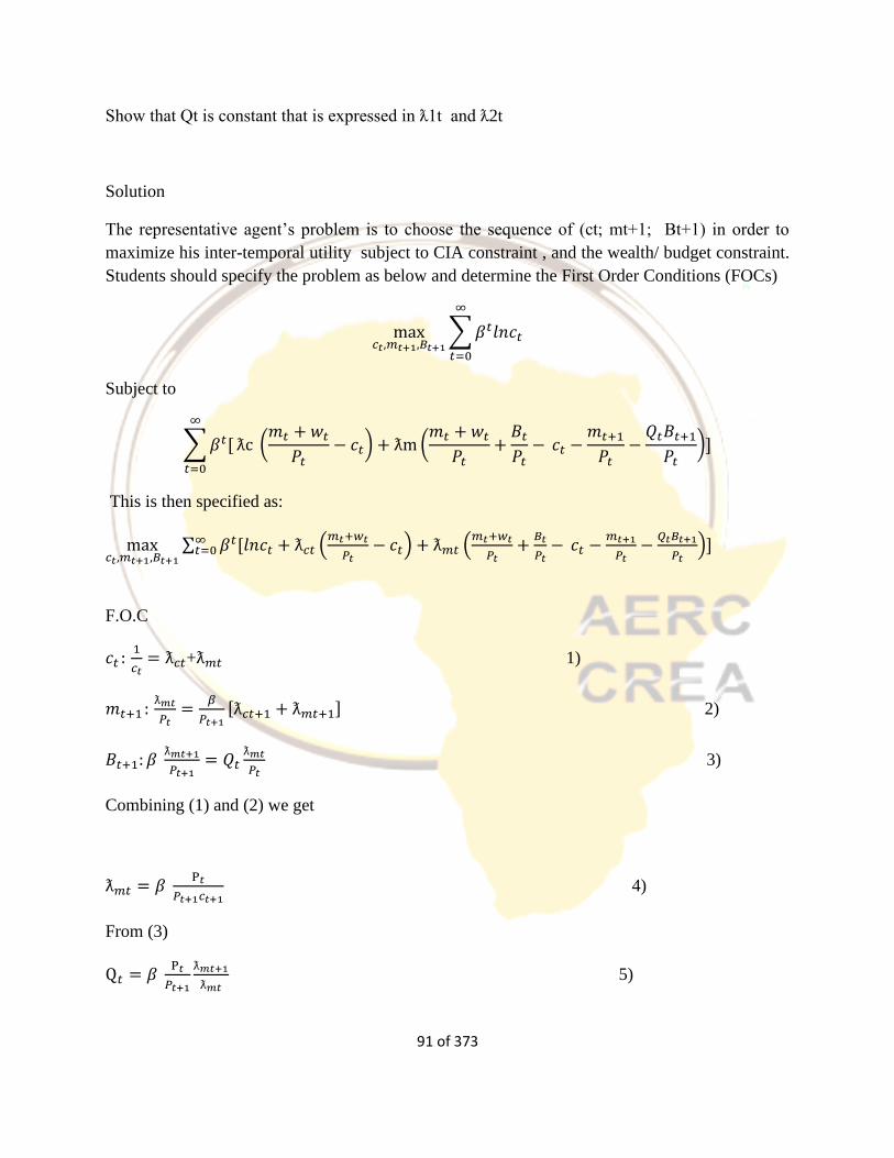
91 of 373

Show that Qt is constant that is expressed in ƛ1t and ƛ2t

Solution

The representative agent’s problem is to choose the sequence of (ct; mt+1; Bt+1) in order to

maximize his inter-temporal utility subject to CIA constraint , and the wealth/ budget constraint.

Students should specify the problem as below and determine the First Order Conditions (FOCs)

max𝑐𝑡,𝑚𝑡+1,𝐵𝑡+1

∑ 𝛽𝑡𝑙𝑛𝑐𝑡

∞

𝑡=0

Subject to

∑ 𝛽𝑡[

∞

𝑡=0

ƛc (𝑚𝑡 + 𝑤𝑡

𝑃𝑡− 𝑐𝑡) + ƛm (

𝑚𝑡 + 𝑤𝑡

𝑃𝑡+

𝐵𝑡

𝑃𝑡− 𝑐𝑡 −

𝑚𝑡+1

𝑃𝑡−

𝑄𝑡𝐵𝑡+1

𝑃𝑡)]

This is then specified as:

max𝑐𝑡,𝑚𝑡+1,𝐵𝑡+1

∑ 𝛽𝑡[𝑙𝑛𝑐𝑡 + ƛ𝑐𝑡 (𝑚𝑡+𝑤𝑡

𝑃𝑡− 𝑐𝑡) + ƛ𝑚𝑡 (

𝑚𝑡+𝑤𝑡

𝑃𝑡+

𝐵𝑡

𝑃𝑡− 𝑐𝑡 −

𝑚𝑡+1

𝑃𝑡−

𝑄𝑡𝐵𝑡+1

𝑃𝑡)]∞

𝑡=0

F.O.C

𝑐𝑡 : 1

𝑐𝑡= ƛ𝑐𝑡+ƛ𝑚𝑡 1)

𝑚𝑡+1 : ƛ𝑚𝑡

𝑃𝑡=

𝛽

𝑃𝑡+1[ƛ𝑐𝑡+1 + ƛ𝑚𝑡+1] 2)

𝐵𝑡+1: 𝛽 ƛ𝑚𝑡+1

𝑃𝑡+1= 𝑄𝑡

ƛ𝑚𝑡

𝑃𝑡 3)

Combining (1) and (2) we get

ƛ𝑚𝑡 = 𝛽 P𝑡

𝑃𝑡+1𝑐𝑡+1 4)

From (3)

Q𝑡 = 𝛽 P𝑡

𝑃𝑡+1

ƛ𝑚𝑡+1

ƛ𝑚𝑡 5)

92 of 373

Combining (5), (4) and (2), and rewriting (1) as 𝑐𝑡+1 = 1

ƛ𝑚𝑡+1+ƛ𝑐𝑡+1

Q𝑡 =ƛ𝑚𝑡+1

ƛ𝑚𝑡+1 + ƛ𝑐𝑡+1

1.2.9 Overlapping Generation Model

Overlapping generations (OLG) models of money, which was first introduced by Samuelson

(1958), and later with major extensions by Wallace (1980, 1981) have been proposed by some

economists as an alternative to the money in the MIUF). However, other economists do not

consider the OLG models of money in their standard form to be valid or useful for modeling the

actual role of money in the economy.

Basing our presentation on Handa (2009) and the work of Wallace (1980, 1981), we assume the

standard version of the OLG model assumes that the individuals in the economy live for two

periods only – or for two life-stages, “young” and “old,” with each life-stage lasting one period –

and that in each period the economy has two generations of individuals. One of these is the old

generation of individuals who were born in the preceding period and the other is the young

generation born at the beginning of the current period. The old of one generation and the young

of the next one overlap in every period, so that the name given to the models using this

framework is the overlapping generations models.

The OLG framework is a substitute for a timeless or an infinite one, with the representative agent

having an infinite horizon. It does not by itself provide a model, but has to be combined with

other assumptions in order to yield a meaningful model.

The essential assumptions and implications of the OLG models with fiat money

The assumptions of the standard OLG models with money are:

Defining bonds as interest-bearing financial assets that can be used to convey purchasing power

from the present to the future, there are no bonds in the model.

Fiat money is preferable to commodities – and any other assets – as the medium for carrying

forward saving to the following period.

93 of 373

There is net (positive) saving in the first lifestage.

Future periods will not renounce the use of fiat money or pursue policies such that fiat money

will become valueless.

The OLG model’s economy has an infinite horizon, even though the individuals in it have a

finite (two-period) horizon.

Given these assumptions, the OLG models of fiat money explore the value of money for various

growth rates of money versus commodities, growth of population, open market operations, etc.

Among the attractive features claimed for OLG models is that, along certain paths, they establish

a positive value for an intrinsically worthless fiat money10 which is not required by law to be

convertible into commodities, and that time and the distinctiveness of the earning pattern over a

lifetime are incorporated in an “essential” manner.11 Further, they allow for economic agents

who are identical at birth – thus permitting the study of stationary states – while allowing for a

degree of heterogeneity among the economic agents alive at any time in the economy, and also

allow – indeed require – the economy to continue indefinitely into the future.

As pointed out already, OLG models with money generate a zero value of money in the current

period if the value of money is expected to be zero in some future period. This is a characteristic

of bootstrap or bubble paths, which are paths along which the values of the variables depend

upon expected values, even if arbitrary ones, in the future and change if the latter change. The

numerous equilibria of this kind are among the tenuous kind, meaning by this that they are not

based on the fundamentals of the system. However, the usual focus of OLG models is not on

such bootstrap or bubble paths. Rather, their implications are normally analyzed only for the

stationary states of the economy, with expectations assumed to be identical with the stationary

values or with those implied by the rational expectations hypothesis (REH)

The Basic OLG Model

In the standard version of the OLG framework, individuals live for two periods – that is, go

through two life-stages – only. They are often labeled “young” in their first lifestage and “old”

in their second lifestage. This book uses the superscripts y and o to indicate the individual’s

respective life-stages.

94 of 373

For the economy, the periods are t +i, i = 0,1,2, . . .. Period t is the initial period of the analysis

and its old generation is called the “initial old,” whose members were born in period t −1.

Generations born in periods 0,1,2, . . ., will be called the “future generations” and its members

will be referred to merely as “individuals.” The OLG model starts by endowing the initial old

with the initial stock of money. Further, for the basic OLG model of this chapter, it is assumed

that any increase in the money stock in any period is gratuitously given as a lump-sum transfer to

the old in that period. The next chapter deviates from this assumption to examine the case where

the seigniorage from money creation is used to buy up commodities that are then destroyed,

resulting in a net decrease in the commodities left for consumption in the economy.

The number of individuals born in period t is Nt . In the early parts of the analysis of this section,

this number is assumed to be constant at N over time. Under this assumption, in each period t,

the population of 2N individuals consists of N young individuals and N old individuals.

Each individual is assumed to be given a commodity endowment of W y in the young life-stage

and wo in the old life-stage. W y and wo are in units of the single consumption good, assumed in

the basic model to be non-storable (perishable). Some of the versions of the OLG models assume

that wo is zero, but such an assumption is not essential to the OLG framework.

However, if fiat money is to have value, it is essential to assume that the optimal level of

consumption in old age will exceed wo. This is usually guaranteed by an assumption that

consumption will be the same in each life-stage and that wo < wy, so that the individual must ave

while young to provide for extra consumption in the second period.

Intertemporal Budget Constraint of the Young

In the young life-stage, the representative individual can either consume c y or hold money m

out of his endowments of commodities. His budget constraint for the first/young life-stage is:

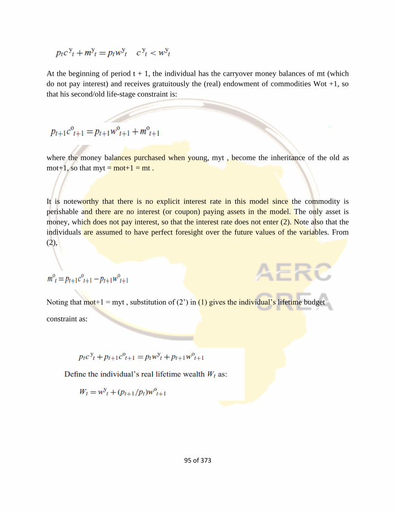
95 of 373

At the beginning of period t + 1, the individual has the carryover money balances of mt (which

do not pay interest) and receives gratuitously the (real) endowment of commodities Wot +1, so

that his second/old life-stage constraint is:

where the money balances purchased when young, myt , become the inheritance of the old as

mot+1, so that myt = mot+1 = mt .

It is noteworthy that there is no explicit interest rate in this model since the commodity is

perishable and there are no interest (or coupon) paying assets in the model. The only asset is

money, which does not pay interest, so that the interest rate does not enter (2). Note also that the

individuals are assumed to have perfect foresight over the future values of the variables. From

(2),

Noting that mot+1 = myt , substitution of (2’) in (1) gives the individual’s lifetime budget

constraint as:

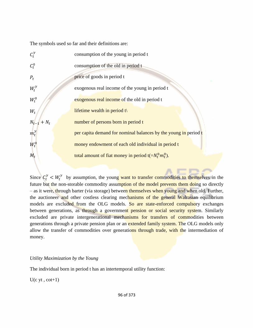
96 of 373

The symbols used so far and their definitions are:

𝐶𝑡𝑦

consumption of the young in period t

𝐶𝑡0 consumption of the old in period t

𝑃𝑡 price of goods in period t

𝑊𝑡𝑦

exogenous real income of the young in period t

𝑊𝑡0 exogenous real income of the old in period t

𝑊𝑡 lifetime wealth in period t\

𝑁𝑡−1 + 𝑁𝑡 number of persons born in period t

𝑚𝑡𝑦

per capita demand for nominal balances by the young in period t

𝑊𝑡0 money endowment of each old individual in period t

𝑀𝑡 total amount of fiat money in period t(=𝑁𝑡0𝑚𝑡

0).

Since 𝐶𝑡𝑦

< 𝑊𝑡𝑦

by assumption, the young want to transfer commodities to themselves in the

future but the non-storable commodity assumption of the model prevents them doing so directly

– as it were, through barter (via storage) between themselves when young and when old. Further,

the auctioneer and other costless clearing mechanisms of the general Walrasian equilibrium

models are excluded from the OLG models. So are state-enforced compulsory exchanges

between generations, as through a government pension or social security system. Similarly

excluded are private intergenerational mechanisms for transfers of commodities between

generations through a private pension plan or an extended family system. The OLG models only

allow the transfer of commodities over generations through trade, with the intermediation of

money.

Utility Maximization by the Young

The individual born in period t has an intertemporal utility function:

U(c yt , cot+1)

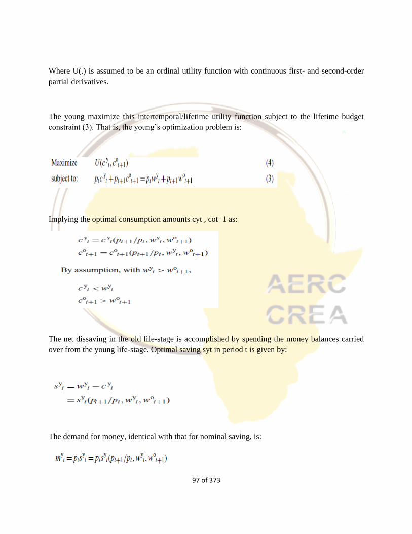
97 of 373

Where U(.) is assumed to be an ordinal utility function with continuous first- and second-order

partial derivatives.

The young maximize this intertemporal/lifetime utility function subject to the lifetime budget

constraint (3). That is, the young’s optimization problem is:

Implying the optimal consumption amounts cyt , cot+1 as:

The net dissaving in the old life-stage is accomplished by spending the money balances carried

over from the young life-stage. Optimal saving syt in period t is given by:

The demand for money, identical with that for nominal saving, is:

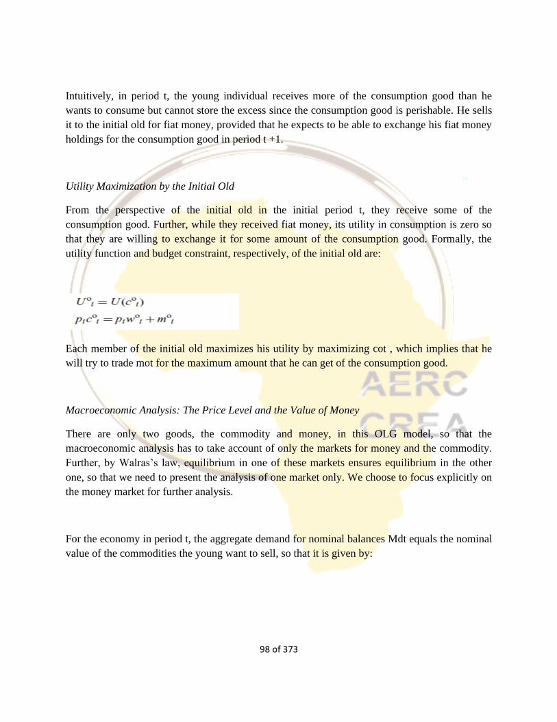
98 of 373

Intuitively, in period t, the young individual receives more of the consumption good than he

wants to consume but cannot store the excess since the consumption good is perishable. He sells

it to the initial old for fiat money, provided that he expects to be able to exchange his fiat money

holdings for the consumption good in period t +1.

Utility Maximization by the Initial Old

From the perspective of the initial old in the initial period t, they receive some of the

consumption good. Further, while they received fiat money, its utility in consumption is zero so

that they are willing to exchange it for some amount of the consumption good. Formally, the

utility function and budget constraint, respectively, of the initial old are:

Each member of the initial old maximizes his utility by maximizing cot , which implies that he

will try to trade mot for the maximum amount that he can get of the consumption good.

Macroeconomic Analysis: The Price Level and the Value of Money

There are only two goods, the commodity and money, in this OLG model, so that the

macroeconomic analysis has to take account of only the markets for money and the commodity.

Further, by Walras’s law, equilibrium in one of these markets ensures equilibrium in the other

one, so that we need to present the analysis of one market only. We choose to focus explicitly on

the money market for further analysis.

For the economy in period t, the aggregate demand for nominal balances Mdt equals the nominal

value of the commodities the young want to sell, so that it is given by:

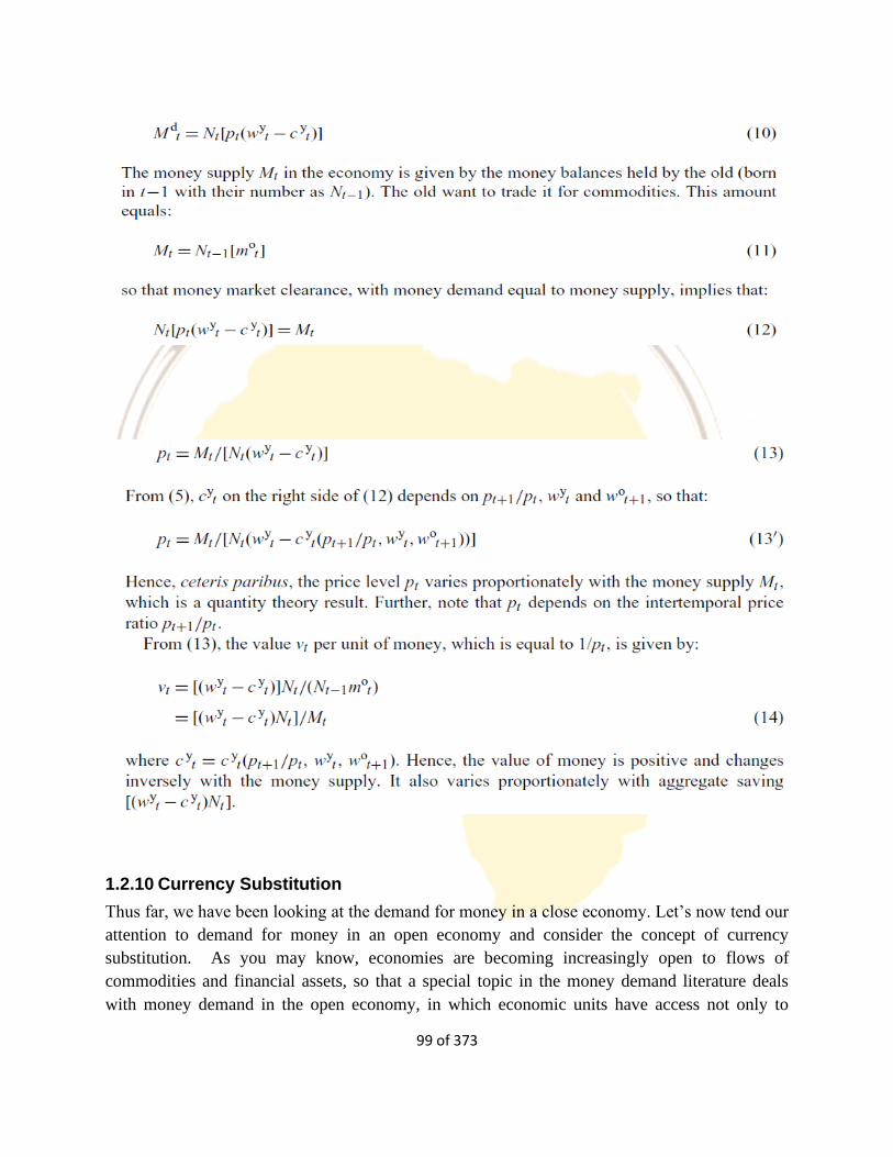
99 of 373

1.2.10 Currency Substitution

Thus far, we have been looking at the demand for money in a close economy. Let’s now tend our

attention to demand for money in an open economy and consider the concept of currency

substitution. As you may know, economies are becoming increasingly open to flows of

commodities and financial assets, so that a special topic in the money demand literature deals

with money demand in the open economy, in which economic units have access not only to

100 of 373

domestic financial assets but also to foreign ones. For portfolio investments in open economies,

the financial alternatives to holding domestic money include the currencies and bonds of foreign

countries, in addition to domestic bonds, so that the determinants of the domestic money demand

should include not only the rates of return on domestic assets but also those on foreign assets.

Since these assets include foreign money holdings, money demand studies for open economies

need to pay special attention to substitution between domestic and foreign monies. This

determination is especially relevant for open economies in which foreign currencies are

extensively traded and foreign monies are part of the domestic media of payments. Note that the

relevant literature on substitution between domestic and foreign money in the open economy

uses the word “currency” for money. In what follows, we follow this usage.

Definition for Currency Substitutions

Currency substitution (CS) can be defined as substitution between domestic and foreign

currencies, which is “currency–currency substitution.” Substitution can also exist between

domestic currency and foreign bonds, and between domestic currency and domestic bonds,

which are “currency–bond substitutions.” Designating, respectively, the nominal values of

domestic money, foreign money, domestic bonds and foreign bonds by M, M∗, B and B∗, CS

can be measured by 𝜕𝑀𝜕𝑀∗⁄ , while the various currency–bond substitutions would be

measured by 𝜕𝑀𝜕𝐵

⁄ , 𝜕𝑀𝜕𝐵∗ ⁄ ∂M∗/∂B and ∂M∗/∂B∗, or by their corresponding elasticities.

Theories of currency substitution

The magnitude of CS will depend both on portfolio selection considerations – since both M and

M∗ are assets in a portfolio26 – and on substitution between them as media of payments in the

domestic economy. Therefore, the relevant approaches to the degree of CS are the portfolio/asset

approach and the transactions approach.

For the asset/portfolio approach, the relevant theory would be the theory of portfolio selection,

which would treat M and M∗ among the assets in the portfolio. This theory would determine

substitution between currencies on the basis of their expected yield and risk. Two currencies

would therefore be perfect substitutes if they had identical returns. They would be poor

substitutes if, with identical risk, the return on one dominated that on the other. This identity of

risk dominance does not in general apply in practice. Note that if some types of bonds were

riskless, then, with a higher return, bonds would dominate over money, so that there would be

zero portfolio demand for currency.

101 of 373

For the transactions approach to the demand for media of payments, it is the general acceptance

in daily exchanges and payments that would determine the degree of substitution

between the alternative assets. If the foreign currencies do serve as a medium of payments in the

domestic economy, the classic demand analysis for the total of the media of payments, i.e. for the

sum of M and M∗, is the Baumol–Tobin inventory analysis presented in an earlier section. Under

this approach, since domestic and foreign bonds do not serve as media of payments they would

have a relatively low substitutability with the domestic currency, while that between M and M∗

could be much higher. Further, the demand for (M +M∗/ρ) would be a function of the domestic

expenditures or GDP to be financed.

For a given amount of transactions or expenditures to be financed, an increase in one medium of

payments implies a decrease in the other, so that transactions demand analysis implies that

∂M/∂(M∗/ρ) < 0. That is, in economies in which both M and M∗ do act as media of payments,

∂M/∂(M∗/ρ) would be negative and significant. In the limit, if domestic residents are indifferent

whether they receive payments in the domestic money or in the foreign one, EM, M∗ = −1,

where EM,M∗ = (M∗/M)(∂M/∂(M∗/ρ)).

This elasticity would be very much smaller in absolute magnitude, or non-existent, in open

economies in which the usage of foreign currency for domestic payments involves significant

additional costs to those for payments in the local currency. If this cost is sufficiently high,

EM, M∗ = 0.

Therefore, the magnitude of EM, M∗ is clearly likely to vary between economies which do not

extensively use foreign monies in domestic payments for goods28 and those economies in which

the foreign money is extensively used as a medium of payments, alongside (or in preference to)

the domestic money.

102 of 373

“Partially dollarized economies” – defined as ones in which the domestic currency and the

foreign one circulate side by side, with buyers and sellers indifferent between their use in settling

transactions – are especially ones in which EM, M∗ tends to −1

Handa (2009) argued that economic agents in even very open economies but without effective

dollarization tend to use the domestic currency as the preferred medium of payments and do not

easily switch to the use of foreign currencies for payments because of the transactions costs30

imposed on retail payments. He therefore designated the domestic currency as being the

“preferred habitat” for the domestic medium of payments. Under this hypothesis, the degree of

substitutability between the domestic currency and a given foreign one would depend on the

latter’s acceptance for payments in the domestic economy or the cost and ease of conversion

from the latter into the former. In general, there would be a very significant transactions cost in

conversion of foreign currencies into the domestic currency. These costs lie in the spread

between the purchase and sale conversion rates and in banks’ commissions, and are usually quite

significant for the size of the transactions of the representative household in the economy.

Further, in retail transactions, payment in a foreign currency is usually at an unfavorable

exchange rate set by the retailer.

Consequently, the general presumption under the preferred habitat approach would be that

foreign currencies will have low elasticities of substitution with the domestic currency, except

possibly in special cases where a particular foreign currency is generally accepted in payments at

par in the domestic economy. To illustrate, while sellers in Canada often accept US dollars, their

offer by buyers is not all that common, because there is a greater cost to paying in the US dollar

than is specified by the bank exchange conversion rate. Hence, under the transactions approach,

the degree of substitution between the US dollar and the Canadian dollar need not be high and

could be quite low. The Canadian dollar finds almost no acceptance in the United States, so they

are poor substitutes in the US economy. Further, in the Canadian economy, even if the Canadian

and US dollars proved to be good substitutes, British currency is not generally accepted and

would be a poor substitute for the Canadian dollar. Most open economies tend to be of this type,

so that, except for special cases, the preferred habitat hypothesis implies that we should expect

even quite open economies (open but without extensive usage of foreign currencies in domestic

retail payments) to have EM ,M∗ close to zero or with a small negative value.

Among the special cases of possibly high CS was the historical use of the local currency and the

imperial one in colonies during the colonial era. Another special case is the use of the US dollar

as a second medium of payments in domestic transactions in partially dollarized economies. For

103 of 373

such economies, the transactions demand for the media of payments implies that, for a given

amount of transactions and GDP to be financed in economies in which both M and M∗ act as

media of payments, a decrease in one would have to be offset by an equivalent increase in the

other. Hence, partially dollarized economies are especially likely to have EM,M∗ equal to –1,

and an infinite elasticity of substitution, while non-dollarized economies will have significantly

lower elasticities of substitution.

Two broad approaches to CS: weak substitutability between monies and bonds

It is an implicit assumption of the CS literature that weak separability exists between the four

financial assets (domestic money, foreign money, domestic bonds and foreign bonds) and other

goods, which include commodities and leisure, so that the demand functions for these four assets

can be estimated by using only the returns on the four financial assets and the amount to be

allocated among them. Proceeding further, the literature allows two possibilities:

A). Preferences over the domestic and foreign monies are not weakly separable from domestic

and foreign bonds. That is, U(M∗, M∗/ρ, B, B∗) is not weakly separable into a sub-function with

M∗ and M∗/ρ. Estimations related to this hypothesis have been labeled in the CS literature the

“unrestricted approach.” As is discussed later, this approach is more suited to the portfolio

approach than to the transactions one. In this approach, the demand function for domestic money

will include the returns on all four assets, in addition to other variables, such as a scale variable.

B) Preferences over domestic and foreign monies are weakly separable from domestic and

foreign bonds. That is,

U(M∗,M/ρ, B, B∗) is weakly separable into a sub-function with M∗ and M∗/ρ, so that:

U(M∗ ,M∗/ρ,B, B∗) = U( f (M,M∗/ρ),B,B∗).

Estimations related to this hypothesis have been labeled the “restricted approach” in the CS

literature. This approach is appropriate for the demand for the two monies as domestic media of

payments. It allows the possibility that domestic money and foreign money may act as media of

104 of 373

payments in the domestic economy, but bonds do not. If this is so, the demand functions for M

and M∗ can be estimated as a function of ρ, the returns on M and M∗ and the amount to be

allocated between them. Such estimation is said to be “restricted,” since it is independent of the

returns on bonds.

1.2.11 Empirical Studies of the Demand for Money with emphasis on Africa

The empirical relationship which has received most attention in the modelling of private sector

financial behaviour is the demand for money function. Over the years, there has been a plethora

of studies on the aggregate demand for money functions of African countries, and it is arguably

the most estimated relationship in the whole of empirical macroeconomics. The majority of these

studies have not been primarily concerned with testing, at the aggregate level, the empirical

validity of the alternative micro theories of money demand. This is partly because total money

holdings are not readily separable into their different transactions, precautionary and risk-return

elements, a degree of disaggregation which is required for the satisfactory testing of most of

these theories. Also, variables such as the risk attached to bond holding, the level of brokerage

costs and the variance of net receipts, which are crucial to the testing of particular theories, are

by their very nature, difficult to measure in any satisfactory way for empirical purposes. These

data limitations have meant that most empirical studies have been concerned with finding a

stable aggregate time-series relationship, between money holdings and a few key determining

variables, such as the rate of interest and the level of income or wealth.

The following empirical studies will be reviewed:

Group Article Title Reference

1 Empirical Analysis of Money Demand Stability in

Nigeria

Osmond N. Okonkwo1*

Emmanuel I. Ajudua Sunny

T. Alozie

Journal of Economics and

Sustainable Development

Vol.5, No.14, 2014

2 Stability Of Money Demand In A Developing

Economy: Empirical Evidence From South Africa

Ferdinand Niyimbanira and

International Business &

105 of 373

Economics Research Journal

– May 2013 Volume 12,

Number 5

3 Some Empirical Evidence on the Stability of Money

Demand in Kenya

Moses C. Kiptui

International Journal of

Economics and Financial

Issues

Vol. 4, No. 4, 2014, pp.849-

858

4 The Stability of the Demand for Money in Monetary

Unions: Some Empirical Evidence from

WAEMU

Pierre Canac , Hassan

Shirvani & Barry Wilbratte

International Economic

Journal

Vol. 23, No. 4, 617–628,

December 2009

5 On the Stability of Money Demand in

Ghana: A Bounds Testing Approach

Jihad Dagher and Arto

Kovanen

IMF Working Paper,

WP/11/273

6

Comparative Analysis of the Stability of Money

Demand between Côte d’Ivoire And Ghana: An

Application of ARDLModel

Yao Kouadio Ange-

Patrick1& Drama Bédi Guy

Hervé

International Journal of

Economics and Finance; Vol.

9, No. 11; 2017

106 of 373

Discussions and Review Questions

Differentiate between the relationship between the rate of interest and the demand for money

within the Keynesian theory of money demand and the classical quantity theory of money

demand?

Discuss the inventory theoretic approach to the transactions demand for money. In which way(s)

is it an improvement over Keynes’s Liquidity Preference model?

Based on the Baumol-Tobin model of the transaction demand for money, assume that a person

has income/expenditure $Y, Bond savings B which earns interest R, money holdings M and cash

bonds cash bonds in lots of $W spaced evenly through the period.

If every withdrawal, he incurs a “brokerage (bonds–money transfer) cost” that has two

components: a fixed cost of $B0 and a variable cost of B1 per dollar withdrawn, derive an

expression for the optimal number of trips (n*) that minimizes the total cost.

Derive the real money demand (the average money holding) function.

With the aid of a diagram show the effect of a fall in interest rate on optimal number of trips (n*)

and average money holding.

Assuming the individual’s objective is to maximize the lifetime utility function:

)()1

1()( 1+

++= t

OY

t CUCUV , θ ≤ 0, uj(·) > 0, ujj(·) < 0.

𝑙𝑛𝐶1𝑡 +1

1 + 𝜌𝑙𝑛𝐶2𝑡+1

If the first stage budget constraint is given as:

Y

tC+ St = Wt

And the second stage budget constraint is given as:

107 of 373

1+tOC = (1 + rt+1) · St;

Where

Y

tC designates the second period consumption of the same generation

1+tOC designates the second period consumption of the same generation;

St designates the savings of the young generation in period t;

Wt designates the wages received by the young generation in t.

= discount factor.

Maximize the individual utility subject to the intertemporal budget constraint and.

Show that that the ratio of the marginal utility of the two goods Y

tCand 1+t

OC (MRS) is a

positive function of interest rt

Suppose that consumption or purchase can only be made in cash so that Cash-in-advance (CIA)

constraint applies only on consumption good. The preference of the representative agent is

given by

𝑈 = ∑ 𝛽𝑡𝑙𝑛𝑐𝑡

∞

𝑡=0

The purchase of consumption good at time t is subject to the CIA constraint

ptct ≤ mt + wt

where Pt is the price of consumption good, Qt is the price of bonds, mt is nominal money

balance that the household carried from the previous period and wt lump-sum-transfer equal to at

the beginning of period t.

The budget constraint for the household in any period t is

mt+1 + QtBt+1 ≤ (mt + wt − ptct) + Bt

where Bt+1 is the total units of nominal bond demanded at time t.

108 of 373

Find the representative agents' optimization problem for (ct; mt+1; Bt+1) in order to maximize

his inter-temporal utility function above subject to the CIA constraint and the wealth constraint.

Show that Qt is constant that is expressed in ƛ1t and ƛ2t

Consider a standard two period OLG model, where the preference function of a household is

given as: 𝑈(𝐶𝑡𝑦

, 𝐶𝑡+10 ) = ln(𝐶𝑡

𝑦) + 𝛽ln (𝐶𝑡+1

0 )

The budget constraints are Wt = Y

tC+ St and 1+t

OC = (1 + rt+1) · St;

Where

Y

tC designates the second period consumption of the same generation

1+tOC designates the second period consumption of the same generation;

St designates the savings of the young generation in period t;

Wt designates the wages received by the young generation in t.

Derive the optimal consumption path, 𝐶𝑡𝑦

𝑎𝑛𝑑 𝐶𝑡+10 , for the individual.

Derive the saving functions for the individual.

Define currency substitution and distinguish it from capital mobility, as well as from substitution

between domestic and foreign bonds. How are the returns on foreign monies and foreign bonds

determined?

109 of 373

1.3 THE SUPPLY OF MONEY

Introduction

In this lecture we are going to explore how changes in the quantity of money occur. Note that

changes or growth of money supply is an important factor not only for acceleration of the

process of economic development but also for the achievement of price stability in the economy.

There must be controlled expansion of money supply if the objective of development with

stability is to be achieved. A healthy growth of an economy requires that there should be neither

inflation nor deflation. Inflation is the greatest headache of a developing economy. A mild

inflation arising out of the creation of money by deficit financing may stimulate investment by

raising profit expectations and extracting forced savings. But a runaway inflation is highly

detrimental to economic growth. The developing economies have to face the problem of

inadequacy of resources in initial stages of development and it can make up this deficiency by

deficit financing. But it has to be kept strictly within safe limits. Thus, increase in money supply

affects vitally the rate of economic growth. In fact, it is now regarded as a legitimate instrument

of economic growth. Kept within proper limits it can accelerate economic growth but exceeding

of the limits will retard it. Thus, management of money supply is essential in the interest of

steady economic growth.

In most countries today, a central bank or other monetary authority is charged with controlling

the stock of money or issuing domestic currency. That is an important charge because the supply

of money greatly influences interest and inflation rates and, ultimately, aggregate output, as

noted earlier. If the central bank’s monetary policy is good, if it creates just the right amount of

money, the economy will hum, and interest and inflation rates will be low. If it creates too much

money too quickly, prices will increase rapidly and wipe out people’s savings until even the

poorest people are nominal billionaires (as in Zimbabwe recently). If it creates too little money

too slowly, prices will fall, wiping out debtors and making it nearly impossible to earn profits in

business (as in the Great Depression). But even less extreme errors can have serious negative

consequences for the economy and hence your wallets, careers, and dreams. This section is a

little involved, but it is worth thoroughly understanding the money supply process and money

multipliers if you want you and yours to be healthy and happy.

By the end of this section, students should be able to:

Explain Money Supply/Stock (including the effects of Financial Innovations)

Describe Endogenous Money Supply: Credit Creation Process

Explain the Monetary Base Model of Money Supply

Explain and distinguish between the Flow of Funds Approach and the Base Multiplier

approaches to Money Supply

Describe the relationship between Fiscal Balance and the Money Supply Process

Describe how empirical studies of money supply are carried out

110 of 373

1.3.1 Money Supply/Stock (including the effects of Financial Innovations)

Money is a good, which, just like other goods, is demanded and supplied by economic agents in

the economy (Handa 2009). There are a number of determinants of the demand and supply of

money. The most important of the determinants of money demand are national income, the price

level and interest rates, while that of money supply is the behavior of the central bank of the

country which is given the power to control the money supply and bring about changes in it. The

equilibrium amount in the market for money specifies the money stock, as opposed to the money

supply, which is a behavioral function specifying the amount that would be supplied at various

interest rates and income levels. The equilibrium amount of money is the amount for which

money demand and money supply are equal.

The money supply and the money stock are identical in the case where the money supply is

exogenously determined, usually by the policies of the central bank. In such a case, it is

independent of the interest rate and other economic variables, though it may influence them.

Much of the monetary and macroeconomic reasoning of a theoretical nature assumes this case,

so that the terms “money stock” and “money supply” are used synonymously. One has to judge

from the context whether the two concepts are being used as distinct or as identical ones. The

control of the money supply rests with the monetary authorities. Their policy with respect to

changes in the money supply is known as monetary policy.

What is relationship between nominal and the real value of money stock?

The nominal value of money is in terms of money itself as the measuring unit. The real value of

money is in terms of its purchasing power over commodities. Thus, the nominal value of a $1

note is 1 – and that of a $20 note is 20. The real value of money is the amount of goods and

services one unit of money can buy and is the reciprocal of the price level of commodities traded

in the economy. It equals 1/P where P is the average price level in the economy. The real value

of money is what we usually mean when we use the term “the value of money.”

Let’s also discuss money and bond markets in monetary macroeconomics. The “money market”

in monetary and macroeconomics is defined as the market in which the demand and supply of

money interact, with equilibrium representing its clearance. However, the common English-

language usage of this term refers to the market for short-term bonds, especially that of Treasury

bills. To illustrate this common usage, this definition is embodied in the term “money market

mutual funds,” which are mutual funds with holdings of short-term bonds. It is important to note

that our usage of the term “the money market” in this book will follow that of macroeconomics.

To reiterate, we will mean by it the market for money, not the market for short-term bonds. The

usual custom in monetary and macroeconomics is to define “bonds” to cover all nonmonetary

financial assets, including loans and shares, so that the words “bonds,” “credit” and “loans” are

treated as synonymous. Given this usage, the “bond/credit/loan market” is defined as the market

for all non-monetary financial assets.

Money supply and Financial innovations

Financial innovation has been extremely rapid since the 1960s. It has included technical changes

in the servicing of various kinds of deposits, such as the introduction of automatic teller

111 of 373

machines, telephone banking, on-line banking through the use of computers, etc. It has\ also

included the creation of new assets such as Money Market Mutual Funds, etc., which are often

sold by banks and can be easily converted into cash. There has also been the spread first of credit

cards, then of debit or bank cards, followed still more recently by the attempts to create and

market “electronic money” cards – sometimes also known as electronic purses or smart cards.

Further, competition among the different types of financial intermediaries in the provision of

liabilities that are close to demand deposits or are readily convertible into the latter, increasingly

by telephone and online banking, has increased considerably in recent decades. Many of these

innovations have further blurred the distinction between demand and savings deposits to the

point of its being only in name rather than in effect, and also blurred the distinction between

banks and some of the other types of financial intermediaries as providers of liquid liabilities.

This process of innovation, and the evolution of financial institutions into an overlapping pattern

in the provision of financial services, are continuing.

Credit cards allow a payer to pay for a purchase while simultaneously acquiring a debt owed to

the credit card company. Because of the latter, most economists choose not to include credit card

usage or their authorized limits in the definition of money. Nor are credit cards near-monies.

However, their usage reduces the need for the purchaser to hold money and reduces the demand

for money. Debit cards are used to pay for purchases by an electronic transfer from the buyer’s

bank account, often a demand deposit account with a bank. They replace the need to make

payments in currency or by issuing a check. Therefore, they reduce currency holdings. They also

reduce payments by checks. However, they do not obviate the need to hold sufficient balances in

the bank account on which the debit is made. They are expected to have a very limited impact on

the holding of deposits, which could increase or decrease.

Electronic transfers are on-line transfers made over the Internet. They reduce the need to use

checks for making payments. However, electronic transfers may not affect deposits in banks, or

do so marginally due to better money-management practices afforded by on-line banking. Smart

cards embody a certain cash value and can be used to make payments at the point of purchase.

Given the increasing prevalence of online banking and debit cards, smart cards are likely to be

mainly used for small payments, as in the case of telephone cards, library photo-copying cards,

etc. Smart cards reduce the need to hold currency and reduce its demand. Therefore, financial

innovations in the form of debit and smart cards reduce currency holdings rather than demand

deposits. Financial innovations in the form of online transfers facilitate the investment of spare

balances, which at one time may have been held in savings deposits, in higher-interest money

market funds, etc., thereby reducing the demand for savings deposits.

In recent decades, the reduction in brokerage fees for transfers between money and nonmonetary

financial assets (bonds and stocks) and the Internet revolution in electronic banking have meant a

reduction in the demand for money. Part of this is due to a reduction in the demand for

precautionary balances held against unexpected consumption expenditures. This reduction has

taken place because individuals can more easily and at lower cost accommodate unexpected

expenditure needs by switching out of other assets into money.

112 of 373

1.3.2 Endogenous Money Supply: Credit Creation Process

Before we begin the money supply or credit creation process, let me take a moment to walk you

through the fundamentals of the central bank balance sheet and the key players involved in the

money supply process. The money supply is determined by the interaction of four groups:

commercial banks and other depositories, depositors, borrowers, and the central bank. Like any

bank, the central bank’s balance sheet is composed of assets and liabilities. Its assets are similar

to those of common banks and include government securities. The central bank’s liabilities,

however, differ fundamentally from those of common banks.

Its most important liabilities are currency in circulation and reserves. It may seem strange to see

currency and reserves listed as liabilities of the central bank because those things are the assets of

commercial banks. In fact, for everyone but the central bank, the central bank’s notes are assets

or things owned. But for the central bank, its notes are things owed (liabilities). Every financial

asset is somebody else’s liability, of course. A promissory note (IOU) that you signed would be

your liability, but it would be an asset for the note’s holder or owner. Similarly, a bank deposit is

a liability for the bank but an asset for the depositor. In like fashion, commercial banks own their

deposits in the central bank (CB) (reserves), so they count them as assets. The CB owes that

money to commercial banks, so it must count them as liabilities. The same goes for banknotes:

the public owns them, but the CB, as their issuer, owes them. (Don’t be confused by the fact that

what the CB owes to holders is nothing more than the right to use the notes to pay sums the

holders owe to the government for taxes and the like.)

Currency in circulation (C) and reserves (R) compose the monetary base (MB, aka high-powered

money), the most basic building blocks of the money supply. Basically, MB = C + R, an

equation you’ll want to internalize. In most countries, C includes banknotes and coins issued by

the the Treasury. We can ignore the latter because it is a relatively small percentage of the MB,

and the Treasury cannot legally manage the volume of coinage in circulation in an active fashion,

but rather only meets the demand for each denomination: .01, .05, .10, .25, .50, and 1.00 coins.

(The CB also supplies the $1.00 unit, and for some reason Americans, for example, prefer $1

notes to coins. In most countries, coins fill demand for the single currency unit denomination.) C

includes only banknotes and coins in the hands of nonbanks. Any banknotes in banks is called

vault cash and is included in R, which also includes bank deposits with the CB. Reserves are of

two types: those required or mandated by the central bank (RR), and any additional or excess

reserves (ER) that banks wish to hold. The latter are usually small, but they can grow

substantially during panics like that of September–October 2008 global financial crisis.

Central banks, of course, are highly profitable institutions because their assets earn interest but

their liabilities are costless, or nearly so. Printing money en masse with modern technology is

pretty cheap, and reserves are nothing more than accounting entries. Many central banks,

including the CB, now pay interest on reserves, but of course any interest paid is composed of

cheap notes or, more likely, even cheaper accounting entries. Central banks, therefore, have no

gap problems, and liquidity management is a snap because they can always print more notes or

create more reserves. Central banks anachronistically own prodigious quantities of gold, but

some have begun to sell off their holdings because they no longer convert their notes into gold or

anything else for that matter. Gold is no longer part of the MB but is rather just a commodity

with unusually good monetary characteristics (high value-to-weight ratio, divisible, easily

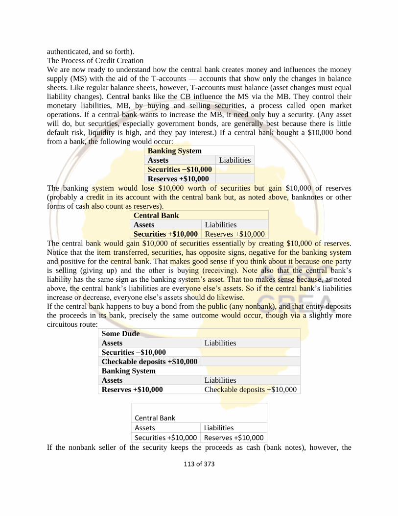
113 of 373

authenticated, and so forth).

The Process of Credit Creation

We are now ready to understand how the central bank creates money and influences the money

supply (MS) with the aid of the T-accounts — accounts that show only the changes in balance

sheets. Like regular balance sheets, however, T-accounts must balance (asset changes must equal

liability changes). Central banks like the CB influence the MS via the MB. They control their

monetary liabilities, MB, by buying and selling securities, a process called open market

operations. If a central bank wants to increase the MB, it need only buy a security. (Any asset

will do, but securities, especially government bonds, are generally best because there is little

default risk, liquidity is high, and they pay interest.) If a central bank bought a $10,000 bond

from a bank, the following would occur:

Banking System

Assets Liabilities

Securities −$10,000

Reserves +$10,000

The banking system would lose $10,000 worth of securities but gain $10,000 of reserves

(probably a credit in its account with the central bank but, as noted above, banknotes or other

forms of cash also count as reserves).

Central Bank

Assets Liabilities

Securities +$10,000 Reserves +$10,000

The central bank would gain $10,000 of securities essentially by creating $10,000 of reserves.

Notice that the item transferred, securities, has opposite signs, negative for the banking system

and positive for the central bank. That makes good sense if you think about it because one party

is selling (giving up) and the other is buying (receiving). Note also that the central bank’s

liability has the same sign as the banking system’s asset. That too makes sense because, as noted

above, the central bank’s liabilities are everyone else’s assets. So if the central bank’s liabilities

increase or decrease, everyone else’s assets should do likewise.

If the central bank happens to buy a bond from the public (any nonbank), and that entity deposits

the proceeds in its bank, precisely the same outcome would occur, though via a slightly more

circuitous route:

Some Dude

Assets Liabilities

Securities −$10,000

Checkable deposits +$10,000

Banking System

Assets Liabilities

Reserves +$10,000 Checkable deposits +$10,000

Central Bank

Assets Liabilities

Securities +$10,000 Reserves +$10,000 If the nonbank seller of the security keeps the proceeds as cash (bank notes), however, the

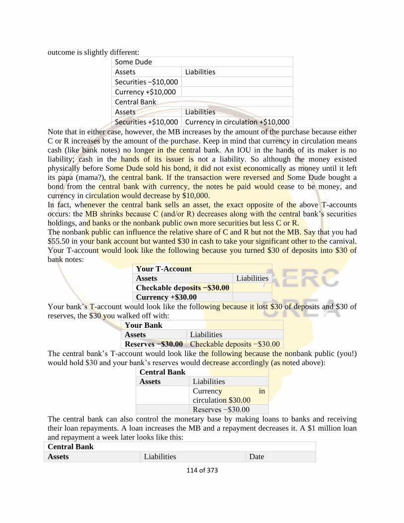
114 of 373

outcome is slightly different:

Some Dude

Assets Liabilities

Securities −$10,000

Currency +$10,000

Central Bank

Assets Liabilities

Securities +$10,000 Currency in circulation +$10,000 Note that in either case, however, the MB increases by the amount of the purchase because either

C or R increases by the amount of the purchase. Keep in mind that currency in circulation means

cash (like bank notes) no longer in the central bank. An IOU in the hands of its maker is no

liability; cash in the hands of its issuer is not a liability. So although the money existed

physically before Some Dude sold his bond, it did not exist economically as money until it left

its papa (mama?), the central bank. If the transaction were reversed and Some Dude bought a

bond from the central bank with currency, the notes he paid would cease to be money, and

currency in circulation would decrease by $10,000.

In fact, whenever the central bank sells an asset, the exact opposite of the above T-accounts

occurs: the MB shrinks because C (and/or R) decreases along with the central bank’s securities

holdings, and banks or the nonbank public own more securities but less C or R.

The nonbank public can influence the relative share of C and R but not the MB. Say that you had

$55.50 in your bank account but wanted $30 in cash to take your significant other to the carnival.

Your T-account would look like the following because you turned $30 of deposits into $30 of

bank notes:

Your T-Account

Assets Liabilities

Checkable deposits −$30.00

Currency +$30.00

Your bank’s T-account would look like the following because it lost $30 of deposits and $30 of

reserves, the $30 you walked off with:

Your Bank

Assets Liabilities

Reserves −$30.00 Checkable deposits −$30.00

The central bank’s T-account would look like the following because the nonbank public (you!)

would hold $30 and your bank’s reserves would decrease accordingly (as noted above):

Central Bank

Assets Liabilities Currency in

circulation $30.00 Reserves −$30.00

The central bank can also control the monetary base by making loans to banks and receiving

their loan repayments. A loan increases the MB and a repayment decreases it. A $1 million loan

and repayment a week later looks like this:

Central Bank

Assets Liabilities Date

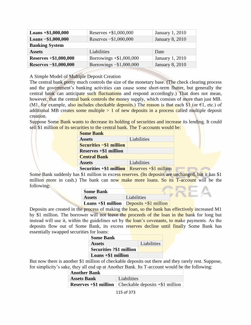
115 of 373

Loans +$1,000,000 Reserves +$1,000,000 January 1, 2010

Loans −$1,000,000 Reserves −$1,000,000 January 8, 2010

Banking System

Assets Liabilities Date

Reserves +$1,000,000 Borrowings +$1,000,000 January 1, 2010

Reserves −$1,000,000 Borrowings −$1,000,000 January 8, 2010

A Simple Model of Multiple Deposit Creation

The central bank pretty much controls the size of the monetary base. (The check clearing process

and the government’s banking activities can cause some short-term flutter, but generally the

central bank can anticipate such fluctuations and respond accordingly.) That does not mean,

however, that the central bank controls the money supply, which consists of more than just MB.

(M1, for example, also includes checkable deposits.) The reason is that each $1 (or €1, etc.) of

additional MB creates some multiple > 1 of new deposits in a process called multiple deposit

creation.

Suppose Some Bank wants to decrease its holding of securities and increase its lending. It could

sell $1 million of its securities to the central bank. The T-accounts would be:

Some Bank

Assets Liabilities

Securities −$1 million

Reserves +$1 million

Central Bank

Assets Liabilities

Securities +$1 million Reserves +$1 million

Some Bank suddenly has $1 million in excess reserves. (Its deposits are unchanged, but it has $1

million more in cash.) The bank can now make more loans. So its T-account will be the

following:

Some Bank

Assets Liabilities

Loans +$1 million Deposits +$1 million

Deposits are created in the process of making the loan, so the bank has effectively increased M1

by $1 million. The borrower will not leave the proceeds of the loan in the bank for long but

instead will use it, within the guidelines set by the loan’s covenants, to make payments. As the

deposits flow out of Some Bank, its excess reserves decline until finally Some Bank has

essentially swapped securities for loans:

Some Bank

Assets Liabilities

Securities ?$1 million

Loans +$1 million

But now there is another $1 million of checkable deposits out there and they rarely rest. Suppose,

for simplicity’s sake, they all end up at Another Bank. Its T-account would be the following:

Another Bank

Assets Bank Liabilities

Reserves +$1 million Checkable deposits +$1 million

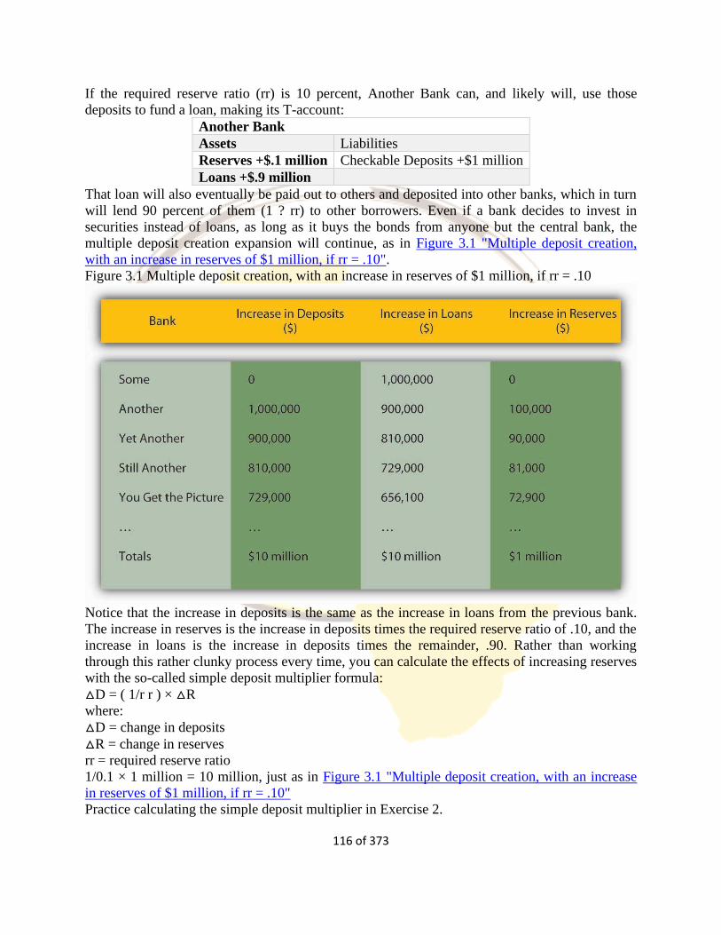
116 of 373

If the required reserve ratio (rr) is 10 percent, Another Bank can, and likely will, use those

deposits to fund a loan, making its T-account:

Another Bank

Assets Liabilities

Reserves +$.1 million Checkable Deposits +$1 million

Loans +$.9 million

That loan will also eventually be paid out to others and deposited into other banks, which in turn

will lend 90 percent of them (1 ? rr) to other borrowers. Even if a bank decides to invest in

securities instead of loans, as long as it buys the bonds from anyone but the central bank, the

multiple deposit creation expansion will continue, as in Figure 3.1 "Multiple deposit creation,

with an increase in reserves of $1 million, if rr = .10".

Figure 3.1 Multiple deposit creation, with an increase in reserves of $1 million, if rr = .10

Notice that the increase in deposits is the same as the increase in loans from the previous bank.

The increase in reserves is the increase in deposits times the required reserve ratio of .10, and the

increase in loans is the increase in deposits times the remainder, .90. Rather than working

through this rather clunky process every time, you can calculate the effects of increasing reserves

with the so-called simple deposit multiplier formula:

△D = ( 1/r r ) × △R

where:

△D = change in deposits

△R = change in reserves

rr = required reserve ratio

1/0.1 × 1 million = 10 million, just as in Figure 3.1 "Multiple deposit creation, with an increase

in reserves of $1 million, if rr = .10"

Practice calculating the simple deposit multiplier in Exercise 2.

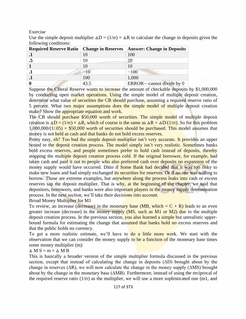
117 of 373

Exercise

Use the simple deposit multiplier △D = (1/rr) × △R to calculate the change in deposits given the

following conditions:

Required Reserve Ratio Change in Reserves Answer: Change in Deposits

.1 10 100

.5 10 20

1 10 10

.1 −10 −100

.1 100 1,000

0 43.5 ERROR—cannot divide by 0

Suppose the CBeral Reserve wants to increase the amount of checkable deposits by $1,000,000

by conducting open market operations. Using the simple model of multiple deposit creation,

determine what value of securities the CB should purchase, assuming a required reserve ratio of

5 percent. What two major assumptions does the simple model of multiple deposit creation

make? Show the appropriate equation and work.

The CB should purchase $50,000 worth of securities. The simple model of multiple deposit

creation is △D = (1/rr) × △R, which of course is the same as △R = △D/(1/rr). So for this problem

1,000,000/(1/.05) = $50,000 worth of securities should be purchased. This model assumes that

money is not held as cash and that banks do not hold excess reserves.

Pretty easy, eh? Too bad the simple deposit multiplier isn’t very accurate. It provides an upper

bound to the deposit creation process. The model simply isn’t very realistic. Sometimes banks

hold excess reserves, and people sometimes prefer to hold cash instead of deposits, thereby

stopping the multiple deposit creation process cold. If the original borrower, for example, had

taken cash and paid it out to people who also preferred cash over deposits no expansion of the

money supply would have occurred. Ditto if Some Bank had decided that it was too risky to

make new loans and had simply exchanged its securities for reserves. Or if no one was willing to

borrow. Those are extreme examples, but anywhere along the process leaks into cash or excess

reserves sap the deposit multiplier. That is why, at the beginning of the chapter, we said that

depositors, borrowers, and banks were also important players in the money supply determination

process. In the next section, we’ll take their decisions into account.

Broad Money Multiplier for M1

To review, an increase (decrease) in the monetary base (MB, which = C + R) leads to an even

greater increase (decrease) in the money supply (MS, such as M1 or M2) due to the multiple

deposit creation process. In the previous section, you also learned a simple but unrealistic upper-

bound formula for estimating the change that assumed that banks hold no excess reserves and

that the public holds no currency.

To get a more realistic estimate, we’ll have to do a little more work. We start with the

observation that we can consider the money supply to be a function of the monetary base times

some money multiplier (m):

△ M S = m × △ M B

This is basically a broader version of the simple multiplier formula discussed in the previous

section, except that instead of calculating the change in deposits (ΔD) brought about by the

change in reserves (ΔR), we will now calculate the change in the money supply (ΔMS) brought

about by the change in the monetary base (ΔMB). Furthermore, instead of using the reciprocal of

the required reserve ratio (1/rr) as the multiplier, we will use a more sophisticated one (m1, and

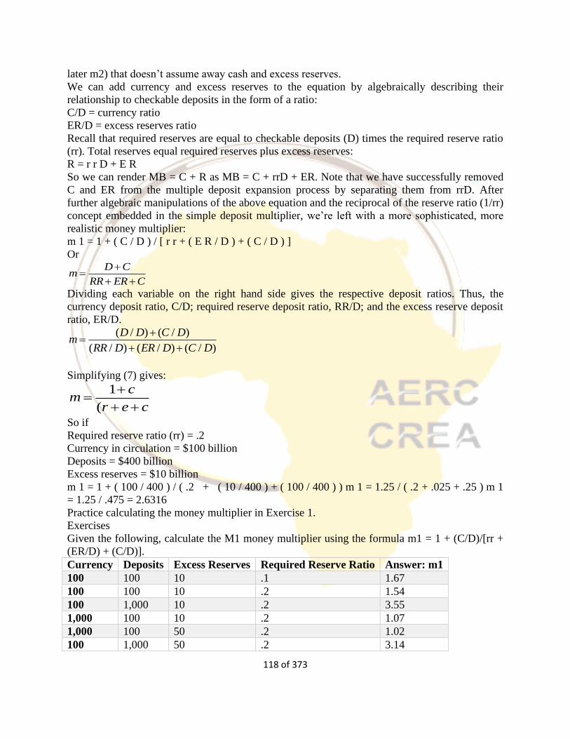
118 of 373

later m2) that doesn’t assume away cash and excess reserves.

We can add currency and excess reserves to the equation by algebraically describing their

relationship to checkable deposits in the form of a ratio:

C/D = currency ratio

ER/D = excess reserves ratio

Recall that required reserves are equal to checkable deposits (D) times the required reserve ratio

(rr). Total reserves equal required reserves plus excess reserves:

R = r r D + E R

So we can render MB = C + R as MB = C + rrD + ER. Note that we have successfully removed

C and ER from the multiple deposit expansion process by separating them from rrD. After

further algebraic manipulations of the above equation and the reciprocal of the reserve ratio (1/rr)

concept embedded in the simple deposit multiplier, we’re left with a more sophisticated, more

realistic money multiplier:

m 1 = 1 + ( C / D ) / [ r r + ( E R / D ) + ( C / D ) ]

Or D C

mRR ER C

+=

+ + Dividing each variable on the right hand side gives the respective deposit ratios. Thus, the

currency deposit ratio, C/D; required reserve deposit ratio, RR/D; and the excess reserve deposit

ratio, ER/D.

( / ) ( / )

( / ) ( / ) ( / )

D D C Dm

RR D ER D C D

+=

+ +

Simplifying (7) gives:

1

(

cm

r e c

+=

+ + So if

Required reserve ratio (rr) = .2

Currency in circulation = $100 billion

Deposits = $400 billion

Excess reserves = $10 billion

m 1 = 1 + ( 100 / 400 ) / ( .2 + ( 10 / 400 ) + ( 100 / 400 ) ) m 1 = 1.25 / ( .2 + .025 + .25 ) m 1

= 1.25 / .475 = 2.6316

Practice calculating the money multiplier in Exercise 1.

Exercises

Given the following, calculate the M1 money multiplier using the formula m1 = 1 + (C/D)/[rr +

(ER/D) + (C/D)].

Currency Deposits Excess Reserves Required Reserve Ratio Answer: m1

100 100 10 .1 1.67

100 100 10 .2 1.54

100 1,000 10 .2 3.55

1,000 100 10 .2 1.07

1,000 100 50 .2 1.02

100 1,000 50 .2 3.14

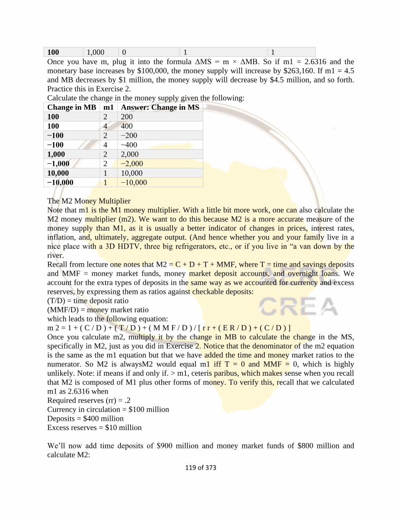
119 of 373

100 1,000 0 1 1

Once you have m, plug it into the formula ΔMS = m × ΔMB. So if m1 = 2.6316 and the

monetary base increases by $100,000, the money supply will increase by $263,160. If m1 = 4.5

and MB decreases by $1 million, the money supply will decrease by $4.5 million, and so forth.

Practice this in Exercise 2.

Calculate the change in the money supply given the following:

Change in MB m1 Answer: Change in MS

100 2 200

100 4 400

−100 2 −200

−100 4 −400

1,000 2 2,000

−1,000 2 −2,000

10,000 1 10,000

−10,000 1 −10,000

The M2 Money Multiplier

Note that m1 is the M1 money multiplier. With a little bit more work, one can also calculate the

M2 money multiplier (m2). We want to do this because M2 is a more accurate measure of the

money supply than M1, as it is usually a better indicator of changes in prices, interest rates,

inflation, and, ultimately, aggregate output. (And hence whether you and your family live in a

nice place with a 3D HDTV, three big refrigerators, etc., or if you live in “a van down by the

river.

Recall from lecture one notes that M2 = C + D + T + MMF, where T = time and savings deposits

and MMF = money market funds, money market deposit accounts, and overnight loans. We

account for the extra types of deposits in the same way as we accounted for currency and excess

reserves, by expressing them as ratios against checkable deposits:

(T/D) = time deposit ratio

(MMF/D) = money market ratio

which leads to the following equation:

m 2 = 1 + ( C / D ) + ( T / D ) + ( M M F / D ) / [ r r + ( E R / D ) + ( C / D ) ]

Once you calculate m2, multiply it by the change in MB to calculate the change in the MS,

specifically in M2, just as you did in Exercise 2. Notice that the denominator of the m2 equation

is the same as the m1 equation but that we have added the time and money market ratios to the

numerator. So M2 is alwaysM2 would equal m1 iff T = 0 and MMF = 0, which is highly

unlikely. Note: if means if and only if. > m1, ceteris paribus, which makes sense when you recall

that M2 is composed of M1 plus other forms of money. To verify this, recall that we calculated

m1 as 2.6316 when

Required reserves (rr) = .2

Currency in circulation = $100 million

Deposits = $400 million

Excess reserves = $10 million

We’ll now add time deposits of $900 million and money market funds of $800 million and

calculate M2:

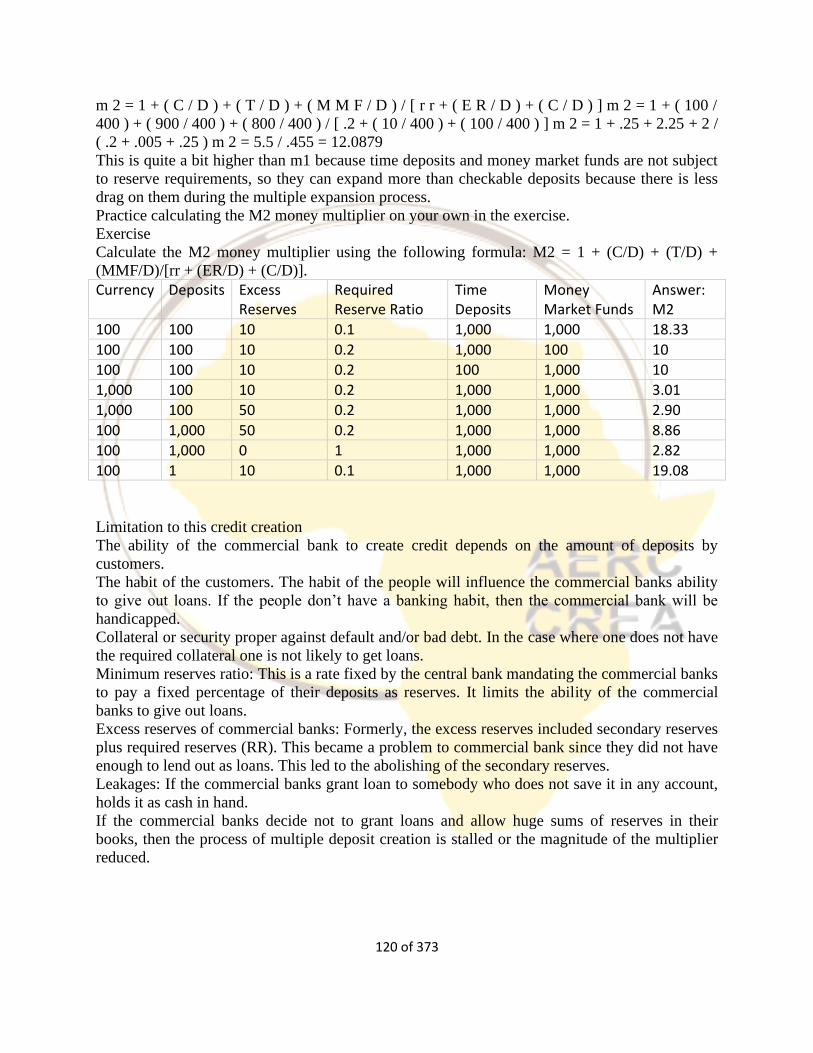
120 of 373

m 2 = 1 + ( C / D ) + ( T / D ) + ( M M F / D ) / [ r r + ( E R / D ) + ( C / D ) ] m 2 = 1 + ( 100 /

400 ) + ( 900 / 400 ) + ( 800 / 400 ) / [ .2 + ( 10 / 400 ) + ( 100 / 400 ) ] m 2 = 1 + .25 + 2.25 + 2 /

( .2 + .005 + .25 ) m 2 = 5.5 / .455 = 12.0879

This is quite a bit higher than m1 because time deposits and money market funds are not subject

to reserve requirements, so they can expand more than checkable deposits because there is less

drag on them during the multiple expansion process.

Practice calculating the M2 money multiplier on your own in the exercise.

Exercise

Calculate the M2 money multiplier using the following formula: M2 = 1 + (C/D) + (T/D) +

(MMF/D)/[rr + (ER/D) + (C/D)].

Currency Deposits Excess Reserves

Required Reserve Ratio

Time Deposits

Money Market Funds

Answer: M2

100 100 10 0.1 1,000 1,000 18.33

100 100 10 0.2 1,000 100 10

100 100 10 0.2 100 1,000 10

1,000 100 10 0.2 1,000 1,000 3.01

1,000 100 50 0.2 1,000 1,000 2.90

100 1,000 50 0.2 1,000 1,000 8.86

100 1,000 0 1 1,000 1,000 2.82

100 1 10 0.1 1,000 1,000 19.08

Limitation to this credit creation

The ability of the commercial bank to create credit depends on the amount of deposits by

customers.

The habit of the customers. The habit of the people will influence the commercial banks ability

to give out loans. If the people don’t have a banking habit, then the commercial bank will be

handicapped.

Collateral or security proper against default and/or bad debt. In the case where one does not have

the required collateral one is not likely to get loans.

Minimum reserves ratio: This is a rate fixed by the central bank mandating the commercial banks

to pay a fixed percentage of their deposits as reserves. It limits the ability of the commercial

banks to give out loans.

Excess reserves of commercial banks: Formerly, the excess reserves included secondary reserves

plus required reserves (RR). This became a problem to commercial bank since they did not have

enough to lend out as loans. This led to the abolishing of the secondary reserves.

Leakages: If the commercial banks grant loan to somebody who does not save it in any account,

holds it as cash in hand.

If the commercial banks decide not to grant loans and allow huge sums of reserves in their

books, then the process of multiple deposit creation is stalled or the magnitude of the multiplier

reduced.

121 of 373

Factors that Determine the Money Multiplier

The Required Reserve Ratio

The Required Reserve Ratio (or the minimum cash reserve ratio or the reserve deposit ratio) is an

important determinant of money supply. An increase in the required reserve ratio reduces the

supply of money with commercial banks and decrease in the required reserve ratio increases

money supply. The RR is the ratio of cash to current and time deposit liabilities which is

determined by law. Every commercial bank is required to keep a certain percentage of these

liabilities in the form of deposits with the central bank of the country. But notes or cash held by

commercial banks in their tills are not included in the minimum required reserve ratio. The

money multiplier and the money supply are negatively related to the required reserve ratio, r.

Currency ration, c

An increase in the currency ratio means that depositors are converting some of their checkable

deposits into currency. As shown earlier, checkable deposits undergo multiple expansions while

currencies do not. Hence when checkable deposits are converted into currency, there is a switch

from a component of the money supply that undergoes multiple expansions to one that does not

undergo multiple expansions. The overall level of multiple expansion declines, and so must the

multiplier. The money multiplier and the money supply are negatively related to the currency

ratio, c.

Excess reserves, e

When banks increase their holdings of excess reserves to checkable deposits, the banking

system, in effect, has fewer reserves to support checkable deposits. This means that given the

same level of H, banks will contract their loans, causing a decline in the level of checkable

deposits and money supply, and the money multiplier will decrease. The money multiplier and

the money supply are negatively related to the excess reserve ratio, e.

b) The cost to a bank of holding excess reserves is its opportunity cost, the interest that could

have been earned on loans or securities it they had been held instead of excess reserves. A

decrease in the interest rate, conversely, will reduce the opportunity cost of excess reserves, and

e will rise.

1.3.3 The Monetary Base Model of Money Supply

The Monetary Base Model, also known as the Base-Multiplier Approach to money supply

determination is an alternative approach to the Flow of Funds approach of money supply which

we will treat in detail in the next section2. The first characteristic of the base-multiplier (B-M)

approach is that it focuses upon stocks. The stocks in question are the stock of monetary base

(M0) and the stock of money (e.g. M4). It points out that the latter is a multiple of the former and

that this multiple is likely to be stable because of two underlying behavioural relationships. Since

2 The notes on these two approaches are based on Bain, K and Howells (2003), Monetary Economics and

its Theoretical Basis, Palgrave, Macmillan, pg 49-70

122 of 373

the components of the monetary base are liabilities of the central bank, the quantity can be varied

at the bank's discretion and, given the stable relationship between M0 and M4, central bank

action on M0 will produce a corresponding (multiple) reaction in M4.

The latter is certainly a powerful insight. After all it says that the stock of money is given by the

size of the base and in the absence of any deliberate decision on the part of the central bank, the

money stock remains constant. It encourages the impression that the monetary authorities are

central and all-powerful in the determination of the money stock because banks’ ability to

acquire non-reserve assets (e.g. loans and advances) are reserve constrained. But we can also see

from this simple summary that this insight depends upon some crucial assumptions about the

underlying system. Firstly, it assumes the stability of two behavioural relationships: indeed, in its

simplest version the B-M approach is sometimes presented as though these relationships are

fixed. But this is an empirical question which needs to be examined.

Secondly, while it is true that the monetary base consists of central bank liabilities, it does not

automatically follow that the central bank either can or even desires to control these liabilities.

Finally, there is a question about whether concentrating on stock equilibrium is very useful when

the underlying variables are subject to continuous change. Put briefly, a monetary system in

which the money supply changes only as the result of the central bank’s deliberate adjustment of

the monetary base, is a system in which the money supply is exogenous — exogenous at least

with respect to the preferences of other agents in the economic system. We turn now to a

more formal examination of the base multiplier approach. We begin by defining the two stocks:

M ≡ Cp + Dp……………………3.1

and

B ≡ Cp + Cb + Db………………3.2

M is (broad) money and consists of notes and coin in circulation with the non-bank public (Cp)

plus their holdings of bank deposits (Dp). In practice, M corresponds to the broad money

measures, the monetary base, consists of those same notes and coin plus also now notes and coin

held by banks (Cb) and banks’ own deposits at the central bank (Db). In practice, B corresponds

to M0. If we now refer to Cb + Db as bank reserves and denote them R, then 3.2 can be rewritten

as:

B ≡ Cp + R ……………………………………..3.3

At any particular time, there will be a monetary base of given value and similarly

a given quantity of broad money and it is a simple task to create a ratio of money to base:

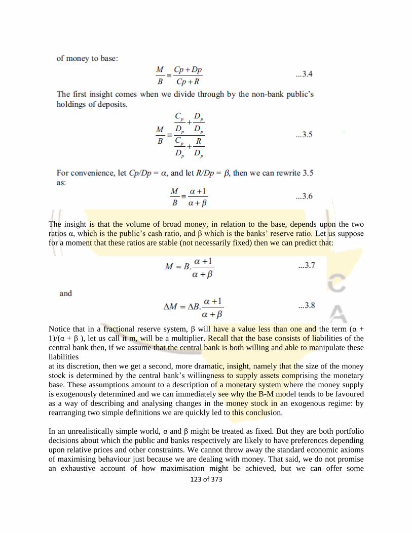
123 of 373

The insight is that the volume of broad money, in relation to the base, depends upon the two

ratios α, which is the public’s cash ratio, and β which is the banks’ reserve ratio. Let us suppose

for a moment that these ratios are stable (not necessarily fixed) then we can predict that:

Notice that in a fractional reserve system, β will have a value less than one and the term (α +

1)/(α + β ), let us call it m, will be a multiplier. Recall that the base consists of liabilities of the

central bank then, if we assume that the central bank is both willing and able to manipulate these

liabilities

at its discretion, then we get a second, more dramatic, insight, namely that the size of the money

stock is determined by the central bank’s willingness to supply assets comprising the monetary

base. These assumptions amount to a description of a monetary system where the money supply

is exogenously determined and we can immediately see why the B-M model tends to be favoured

as a way of describing and analysing changes in the money stock in an exogenous regime: by

rearranging two simple definitions we are quickly led to this conclusion.

In an unrealistically simple world, α and β might be treated as fixed. But they are both portfolio

decisions about which the public and banks respectively are likely to have preferences depending

upon relative prices and other constraints. We cannot throw away the standard economic axioms

of maximising behaviour just because we are dealing with money. That said, we do not promise

an exhaustive account of how maximisation might be achieved, but we can offer some

124 of 373

illustration of relevant factors which will bear upon preferences. If we take α, the public’s cash

ratio, we can say firstly that the decision to divide money holdings between notes and coin

(‘cash’) and bank deposits must surely depend upon any rate of interest paid on deposits,

money’s ‘own rate’, which we might denote im. The higher the rate paid on deposits (and the

wider the range of deposits on which it is paid), the less willing, ceteris paribus, people will be to

hold cash.

Furthermore, one of the reasons for holding deposits is to have access to the payments

mechanism. Just how attractive deposits are as a means of payment depends upon current usage

— many fewer transactions involved bank deposits a hundred years ago than they do now — and

this depends to some extent upon technological considerations. The widespread use of deposits

as means of payment requires the development of an efficient cheque clearing system. Since the

mid-1960s the big developments in the payments system have involved electronic payments —

automating them first of all so that customers could set up standing order or direct debit

instructions and then making electronic transfers possible, most recently in the form of debit

cards. As the services offered by deposits increase and improve, so they become more attractive

relative to cash.

Technology has almost certainly affected the cash/deposit split through other routes. For a given

level of money’s own rate and a given level of ‘services’ from deposits, the decision about how

much cash to hold must depend to some extent upon the difficulties of switching between cash

and deposits, the so-called ‘shoe leather costs’ based on the idea that replenishing cash balances

involved walking to the bank and standing in a queue. But one of the many achievements of

banking technology has been the development of the cash machine or automated teller machine

(‘ATM’) to give it its proper name. These machines now allow a wide range of routine banking

transactions to be carried out at remote sites like supermarkets, filling stations, shopping malls

and even educational institutions. Given that these facilities make cash replenishment easier, they

encourage people to hold smaller cash balances. The effect is likely to be more marked in

periods

of rapid inflation and high nominal interest rates when the protection of purchasing power

offered by interest-bearing deposits will be greatest.

The two examples of technological change we have given, both tend to reduce the public’s cash

ratio: α gets smaller. This need not be the case a priori. It is conceivable that future technological

changes will push in the opposite direction. This means that we cannot give a definite sign to the

partial derivative of technology (as we could with money’s own rate, for example). In practice,

however, it is very likely that technological changes have acted over the years towards a

reduction in the public’s need to hold cash.

As regards influences upon the public’s cash ratio, therefore, we can surmise

that α will depend to some extent upon at least two factors, money’s

own rate and technological conditions.

125 of 373

When it comes to banks’ decisions about their reserve ratios, therefore, there are numerous

influences at work. Remember that banks are profitseeking firms, that the cash element of

reserves yields no interest and that, in most systems deposits at the central bank are also non-

interest bearing. This means that holding reserves acts like a tax on banking.

Banks’ decisions to hold reserves will depend firstly upon their cost. Where reserves pay no

interest then the cost can be proxied by the return on alternative liquid assets, which might be

proxied by the bond rate, ib. Where reserves do pay interest, then the cost will be the return on

reserves, ir relative to the bond rate. The quantity of reserves held will depend also on the cost of

being short, that is upon the rediscount rate charged for lender of last resort facilities, id. This is

the rate of interest announced periodically, usually monthly, by the central bank. In the UK and

the eurozone it is a rate of interest charged by the central bank on short-dated repurchase deals

with banks, using government bonds as the underlying security. Reserve holdings will also

depend upon any mandatory reserve requirement, RR, and, lastly, upon the variability of inward

and outward flows to which banks are subject, σ. This last factor is relevant because the primary

purpose of reserves is to enable individual banks to meet demands for cash or, more importantly,

for transfers of deposits as customers make payments to customers of other banks or to the

government. The majority of payments are offsetting (payments from bank A to bank B will

roughly cancel); reserves are necessary to meet the balance. Provided this balance is predictable,

the need for reserves will be limited to the predicted net flow. If it is unpredictable, then

additional funds have to be held. The greater the variance (or standard deviation) of the flows,

the greater the margin that will be necessary.

In summary, then:

Given that we now have some idea of the sorts of influences, and the direction of their effect,

upon the ratios α and β, the next obvious question is what effect will changes in α and β have

upon the size of the multiplier expression in 3.7 and 3.8. From there, we can see their effect on

the money

supply.

The answer to the first question lies in the value ‘1’. Because the values of α and β are fractions

(in practice, very small fractions) it is the ‘1’ which gives the expression a multiplier value: the

numerator is bound to be larger than the denominator. Consider now what happens if we change

α and β. If we increase (for example) α, we increase the numerator and denominator

simultaneously and the outcome may therefore appear indeterminate at first glance. But with the

numerator already larger than the denominator by virtue of the ‘1’, any change in a must have a

bigger effect proportionate effect upon the denominator. If we are looking at an increase,

therefore, a given change in α must have a bigger effect upon the denominator than the

126 of 373

numerator and the value of the multiplier will fall. With β, the effect is obvious since it appears

only in the denominator. Any change in β must lead to an inverse change in the value of the

multiplier.

Since the money supply depends upon both the base and the multiplier

we can write:

and since we know (from 3.9 and 3.10) how α and β are likely to respond to a number of

influences, we can substitute into (3.11), to yield a money supply determined as follows:

A change in B is a change in the multiplicand; changes in all other variables cause a change in

the size of the multiplier itself.

We turn now to how this account of money supply determination can be presented

diagrammatically. The account of money supply determination which we have just given is more

familiar than it may seem since it is what is assumed, but rarely spelt out, in money market

diagrams where a vertical money supply curve intersects a downward sloping money demand

curve.

This is what we have drawn in Figure 3.1, though we have given the money supply curve a

positive slope for reasons we return to at the end of this section. Before we do that, let us be

clear how changes in the variables listed in 3.12 will be reflected in the diagram. The horizontal

axis depicts the quantity of money as a stock. In this space, a money supply curve intersects the

horizontal (money) axis at a point where M = m.B (where m is the multiplier). A change in B

changes the point of intersection (the supply curve shifts). The same results from a change in any

of RR, id ir, im, σ, T since these cause a change in the value of the multiplier.

Notice that we have omitted the bond rate, ib, from this list. This is because the bond rate must

appear on the vertical axis. This is because the purpose of drawing the money supply curve in

interest-money space at all is ultimately to discuss money market equilibria, the interaction of

supply and demand. With a downward sloping demand curve in the diagram, the rate on the

vertical axis must be the opportunity cost of holding money. Strictly, in a modern monetary

system, one might argue that this rate ought to be a spread term, representing the difference

between the bond rate (appearing as a proxy for the return on ‘non-money financial assets’ which

agents could hold as an alternative) and money’s own rate (effectively the weighted average rate

on cash and deposits). This is true but does not change the point we are about to make. If we put

a spread term on the vertical axis it remains the case that a rise in bond rate increases the

opportunity

cost of holding money. As the size of the spread increases the quantity of money demanded

declines. The crucial point is that it is the bond rate which must appear on the vertical axis, either

on its own (if money is noninterest bearing) or as part of a spread term.

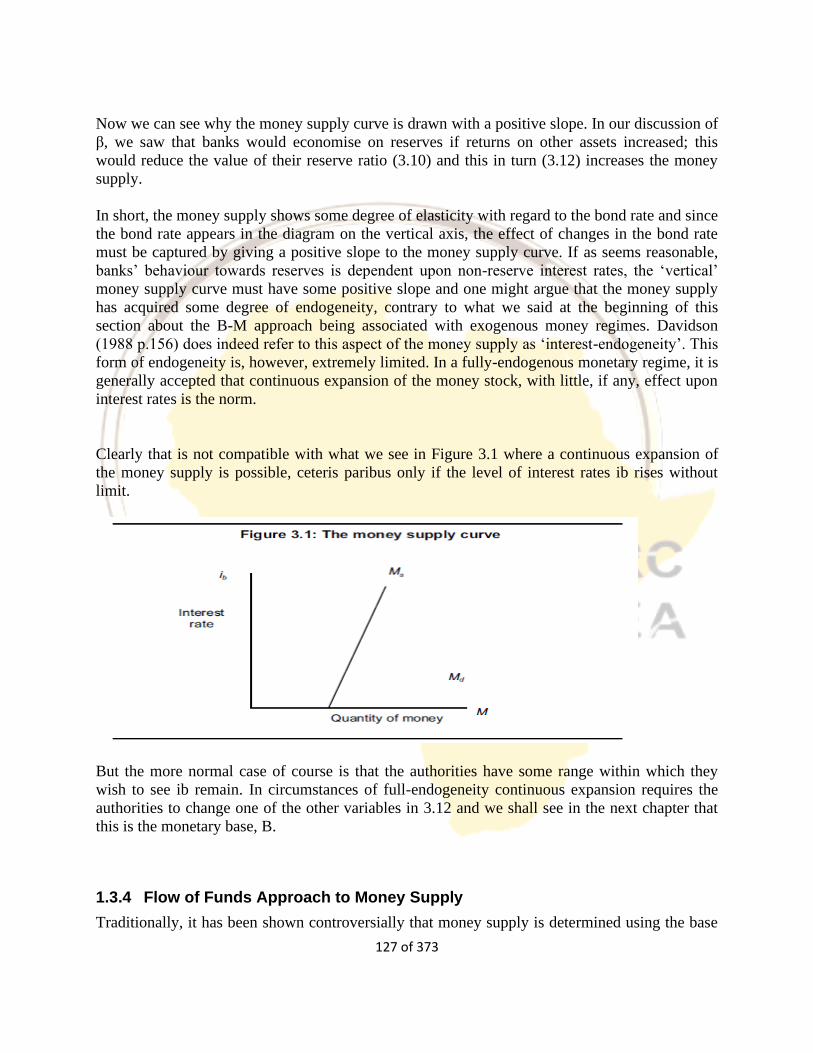
127 of 373

Now we can see why the money supply curve is drawn with a positive slope. In our discussion of

β, we saw that banks would economise on reserves if returns on other assets increased; this

would reduce the value of their reserve ratio (3.10) and this in turn (3.12) increases the money

supply.

In short, the money supply shows some degree of elasticity with regard to the bond rate and since

the bond rate appears in the diagram on the vertical axis, the effect of changes in the bond rate

must be captured by giving a positive slope to the money supply curve. If as seems reasonable,

banks’ behaviour towards reserves is dependent upon non-reserve interest rates, the ‘vertical’

money supply curve must have some positive slope and one might argue that the money supply

has acquired some degree of endogeneity, contrary to what we said at the beginning of this

section about the B-M approach being associated with exogenous money regimes. Davidson

(1988 p.156) does indeed refer to this aspect of the money supply as ‘interest-endogeneity’. This

form of endogeneity is, however, extremely limited. In a fully-endogenous monetary regime, it is

generally accepted that continuous expansion of the money stock, with little, if any, effect upon

interest rates is the norm.

Clearly that is not compatible with what we see in Figure 3.1 where a continuous expansion of

the money supply is possible, ceteris paribus only if the level of interest rates ib rises without

limit.

But the more normal case of course is that the authorities have some range within which they

wish to see ib remain. In circumstances of full-endogeneity continuous expansion requires the

authorities to change one of the other variables in 3.12 and we shall see in the next chapter that

this is the monetary base, B.

1.3.4 Flow of Funds Approach to Money Supply

Traditionally, it has been shown controversially that money supply is determined using the base

128 of 373

multiplier approach, as we have just seen. ‘The multiplier model of the money supply originally

developed by Brunner (1961) and Brunner and Meltzer (1964) has become the standard model to

explain how the policy actions of the Central Bank influence the money stock’. However, there

is more than sufficient evidence to suggest that monetary authorities do not determine the money

supply and that the flow of funds approach makes more sense.

Consequently, I will compare and contrast the base multiplier and the flow of funds approaches

to the determination of money supply and determine which occurs in reality in view of the

present economic climate. As we have just gone through the base-multiplier approach we will

now focus on the flow of funds approach to money supply and later reconcile the two.

Where the base-multiplier approach focused upon stocks, the flow of funds (FoF) approach

concentrates upon changes in stocks, i.e. on flows. There is a connection with the B-M approach

in that one of the flows is the change in money stock; but the other flow which dominates the

FoF approach is the flow of bank lending to the non-bank public. This is strictly speaking the net

change in the stock of bank loans — the difference over time in the stock of loans taking account

of both new loans made and loans repaid. The flow of money is shown as ΔM, the flow of new

loans is shown as ΔLp (for new lending to the non-bank private sector) and ΔLg (for new

lending to the

public sector).1 Because it focuses upon flows of new lending and their ability to create deposits,

the FoF approach is sometimes known as the ‘credit-counterparts’ approach.

As with the B-M approach, we begin with the money supply identity:

M ≡ Cp + Dp ………………………3.13/3.1

and then rewrite it in flows:

ΔM ≡ ΔCp + ΔDp…………..3.14

We next concentrate on the deposit element and use the bank balance sheet identity to remind

ourselves that since deposits (liabilities) must be matched by loans (assets) then the same must

be true about changes. On the asset side, loans can be decomposed into loans to the private and

to the public sector.

ΔDp ≡ ΔLp + ΔLg……………………………………….3.15

Concentrate now on bank loans to the public sector. These are just one way of financing the

public sector and, because of its monetary implications and short-term nature, it tends to be a

residual source of financing — something to be resorted to after all other forms of finance. So it

follows that we can locate the flow of new bank lending to the public sector (PSBR) within the

public sector’s total borrowing requirement:

ΔLg ≡ PSBR − ΔGp − ΔCp ± Δext…………………………3.16

where ΔGp represents net sales of government bonds to the general public. Notice that Δext can

take a positive or negative value. Δext refers to the monetary implications of external flows. For

129 of 373

example, if the public sector buys foreign currency assets with sterling (as it might if it were

trying to hold a fixed exchange rate) this adds to the public sector’s borrowing requirement.

Selling foreign currency assets for sterling reduces the need for sterling borrowing.

We can then substitute 3.16 into 3.15 to show all the sources of change

in deposits:

ΔDp ≡ ΔLp + PSBR − ΔGp − ΔCp ± Δext ………………………...3.17

and then substitute 3.17 into 3.14 to show all sources of monetary change. In making the

substitution we have tidied up (notice that ΔCp cancels because it enters twice, with opposite

signs) and reordered the terms to give 3.18, which is often referred to as the ‘flow of funds

identity’.

ΔM ≡ PSBR − ΔGp ± Δext + ΔLp………………………………………3.18

What insights do we gain from the FoF approach? The explicit message is that changes in the

money stock are inextricably linked to lending/borrowing behaviour. But behind this are three

implications. The first of these is that changes themselves are what matters — one would not use

the FoF approach to analyse a system where stocks dominate everyone’s interest. It is an

implication of the FoF approach that our interest in money supply is an interest in monetary

growth. The second implication is that the monetary base is of little interest. We shall see in the

next section that we can rewrite the flow of funds identity so as to include changes in the

monetary

base, but the fact that the FoF identity is not normally written in that way is significant. One does

not adopt a method of analysis which deliberately omits variables which one thinks are

important.

It points to flows as the important variables and by omitting references to the monetary base it

hints that the authorities might need to find some non-base-orientated way of influencing these

flows. Equally, one does not normally adopt a mode of analysis which gives a key position to

variables of little interest. The third implication of the FoF analysis, therefore, is that if/when the

authorities become interested in the magnitude of flows, they should pay attention to

lending/borrowing. While the B-M approach creates the impression that bank lending is reserve

(supply) constrained, the FoF creates the impression that it is (demand) constrained by the non

bank private sector’s desire for additional credit.

The two approaches compared

While the B-M and FoF approaches are different ways of analysing the quantity of monetary

assets, both consist of rearranging identities at least one of which — the money stock and its

components — is common to both.

In fact, even though each approach offers a different range of insights and highlights different

features of the monetary system as being significant, it is possible to reconcile the two

approaches. Indeed it is perfectly possible to analyse money supply changes or flows by using an

identity which features the monetary base while one could, if one were so inclined, analyse the

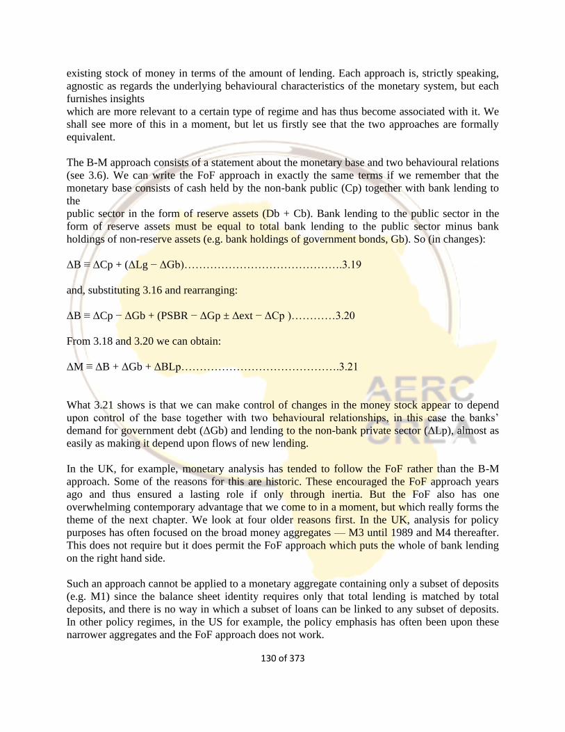
130 of 373

existing stock of money in terms of the amount of lending. Each approach is, strictly speaking,

agnostic as regards the underlying behavioural characteristics of the monetary system, but each

furnishes insights

which are more relevant to a certain type of regime and has thus become associated with it. We

shall see more of this in a moment, but let us firstly see that the two approaches are formally

equivalent.

The B-M approach consists of a statement about the monetary base and two behavioural relations

(see 3.6). We can write the FoF approach in exactly the same terms if we remember that the

monetary base consists of cash held by the non-bank public (Cp) together with bank lending to

the

public sector in the form of reserve assets (Db + Cb). Bank lending to the public sector in the

form of reserve assets must be equal to total bank lending to the public sector minus bank

holdings of non-reserve assets (e.g. bank holdings of government bonds, Gb). So (in changes):

ΔB ≡ ΔCp + (ΔLg − ΔGb)…………………………………….3.19

and, substituting 3.16 and rearranging:

ΔB ≡ ΔCp − ΔGb + (PSBR − ΔGp ± Δext − ΔCp )…………3.20

From 3.18 and 3.20 we can obtain:

ΔM ≡ ΔB + ΔGb + ΔBLp…………………………………….3.21

What 3.21 shows is that we can make control of changes in the money stock appear to depend

upon control of the base together with two behavioural relationships, in this case the banks’

demand for government debt (ΔGb) and lending to the non-bank private sector (ΔLp), almost as

easily as making it depend upon flows of new lending.

In the UK, for example, monetary analysis has tended to follow the FoF rather than the B-M

approach. Some of the reasons for this are historic. These encouraged the FoF approach years

ago and thus ensured a lasting role if only through inertia. But the FoF also has one

overwhelming contemporary advantage that we come to in a moment, but which really forms the

theme of the next chapter. We look at four older reasons first. In the UK, analysis for policy

purposes has often focused on the broad money aggregates — M3 until 1989 and M4 thereafter.

This does not require but it does permit the FoF approach which puts the whole of bank lending

on the right hand side.

Such an approach cannot be applied to a monetary aggregate containing only a subset of deposits

(e.g. M1) since the balance sheet identity requires only that total lending is matched by total

deposits, and there is no way in which a subset of loans can be linked to any subset of deposits.

In other policy regimes, in the US for example, the policy emphasis has often been upon these

narrower aggregates and the FoF approach does not work.

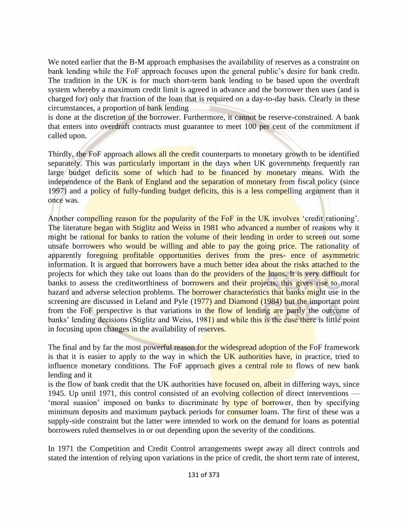
131 of 373

We noted earlier that the B-M approach emphasises the availability of reserves as a constraint on

bank lending while the FoF approach focuses upon the general public’s desire for bank credit.

The tradition in the UK is for much short-term bank lending to be based upon the overdraft

system whereby a maximum credit limit is agreed in advance and the borrower then uses (and is

charged for) only that fraction of the loan that is required on a day-to-day basis. Clearly in these

circumstances, a proportion of bank lending

is done at the discretion of the borrower. Furthermore, it cannot be reserve-constrained. A bank

that enters into overdraft contracts must guarantee to meet 100 per cent of the commitment if

called upon.

Thirdly, the FoF approach allows all the credit counterparts to monetary growth to be identified

separately. This was particularly important in the days when UK governments frequently ran

large budget deficits some of which had to be financed by monetary means. With the

independence of the Bank of England and the separation of monetary from fiscal policy (since

1997) and a policy of fully-funding budget deficits, this is a less compelling argument than it

once was.

Another compelling reason for the popularity of the FoF in the UK involves ‘credit rationing’.

The literature began with Stiglitz and Weiss in 1981 who advanced a number of reasons why it

might be rational for banks to ration the volume of their lending in order to screen out some

unsafe borrowers who would be willing and able to pay the going price. The rationality of

apparently foregoing profitable opportunities derives from the pres- ence of asymmetric

information. It is argued that borrowers have a much better idea about the risks attached to the

projects for which they take out loans than do the providers of the loans. It is very difficult for

banks to assess the creditworthiness of borrowers and their projects, this gives rise to moral

hazard and adverse selection problems. The borrower characteristics that banks might use in the

screening are discussed in Leland and Pyle (1977) and Diamond (1984) but the important point

from the FoF perspective is that variations in the flow of lending are partly the outcome of

banks’ lending decisions (Stiglitz and Weiss, 1981) and while this is the case there is little point

in focusing upon changes in the availability of reserves.

The final and by far the most powerful reason for the widespread adoption of the FoF framework

is that it is easier to apply to the way in which the UK authorities have, in practice, tried to

influence monetary conditions. The FoF approach gives a central role to flows of new bank

lending and it

is the flow of bank credit that the UK authorities have focused on, albeit in differing ways, since

1945. Up until 1971, this control consisted of an evolving collection of direct interventions —

‘moral suasion’ imposed on banks to discriminate by type of borrower, then by specifying

minimum deposits and maximum payback periods for consumer loans. The first of these was a

supply-side constraint but the latter were intended to work on the demand for loans as potential

borrowers ruled themselves in or out depending upon the severity of the conditions.

In 1971 the Competition and Credit Control arrangements swept away all direct controls and

stated the intention of relying upon variations in the price of credit, the short term rate of interest,

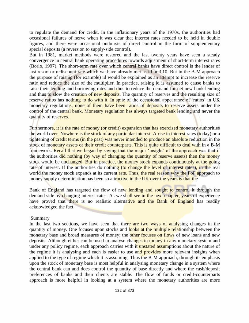
132 of 373

to regulate the demand for credit. In the inflationary years of the 1970s, the authorities had

occasional failures of nerve when it was clear that interest rates needed to be held in double

figures, and there were occasional outbursts of direct control in the form of supplementary

special deposits (a reversion to supply-side control).

But in 1981, market methods were restored and the last twenty years have seen a steady

convergence in central bank operating procedures towards adjustment of short-term interest rates

(Borio, 1997). The short-term rate over which central banks have direct control is the lender of

last resort or rediscount rate which we have already met as id in 3.10. But in the B-M approach

the purpose of raising (for example) id would be explained as an attempt to increase the reserve

ratio and reduce the size of the multiplier. In practice, raising id is assumed to cause banks to

raise their lending and borrowing rates and thus to reduce the demand for net new bank lending

and thus to slow the creation of new deposits. The quantity of reserves and the resulting size of

reserve ratios has nothing to do with it. In spite of the occasional appearance of ‘ratios’ in UK

monetary regulations, none of them have been ratios of deposits to reserve assets under the

control of the central bank. Monetary regulation has always targeted bank lending and never the

quantity of reserves.

Furthermore, it is the rate of money (or credit) expansion that has exercised monetary authorities

the world over. Nowhere is the stock of any particular interest. A rise in interest rates (today) or a

tightening of credit terms (in the past) was never intended to produce an absolute reduction in the

stock of monetary assets or their credit counterparts. This is quite difficult to deal with in a B-M

framework. Recall that we began by saying that the major ‘insight’ of the approach was that if

the authorities did nothing (by way of changing the quantity of reserve assets) then the money

stock would be unchanged. But in practice, the money stock expands continuously at the going

rate of interest. If the authorities do nothing (to change the level of interest rates), in the real

world the money stock expands at its current rate. Thus, the real reason why the FoF approach to

money supply determination has been so attractive in the UK over the years is that the

Bank of England has targeted the flow of new lending and sought to control it through the

demand side by changing interest rates. As we shall see in the next chapter, years of experience

have proved that there is no realistic alternative and the Bank of England has readily

acknowledged the fact.

Summary

In the last two sections, we have seen that there are two ways of analysing changes in the

quantity of money. One focuses upon stocks and looks at the multiple relationship between the

monetary base and broad measures of money; the other focuses on flows of new loans and new

deposits. Although either can be used to analyse changes in money in any monetary system and

under any policy regime, each approach carries with it unstated assumptions about the nature of

the regime it is analysing and each is easier to use and provides more relevant insights when

applied to the type of regime which it is assuming. Thus the B-M approach, through its emphasis

upon the stock of monetary base is most helpful in analysing monetary change in a system where

the central bank can and does control the quantity of base directly and where the cash/deposit

preferences of banks and their clients are stable. The flow of funds or credit-counterparts

approach is more helpful in looking at a system where the monetary authorities are more

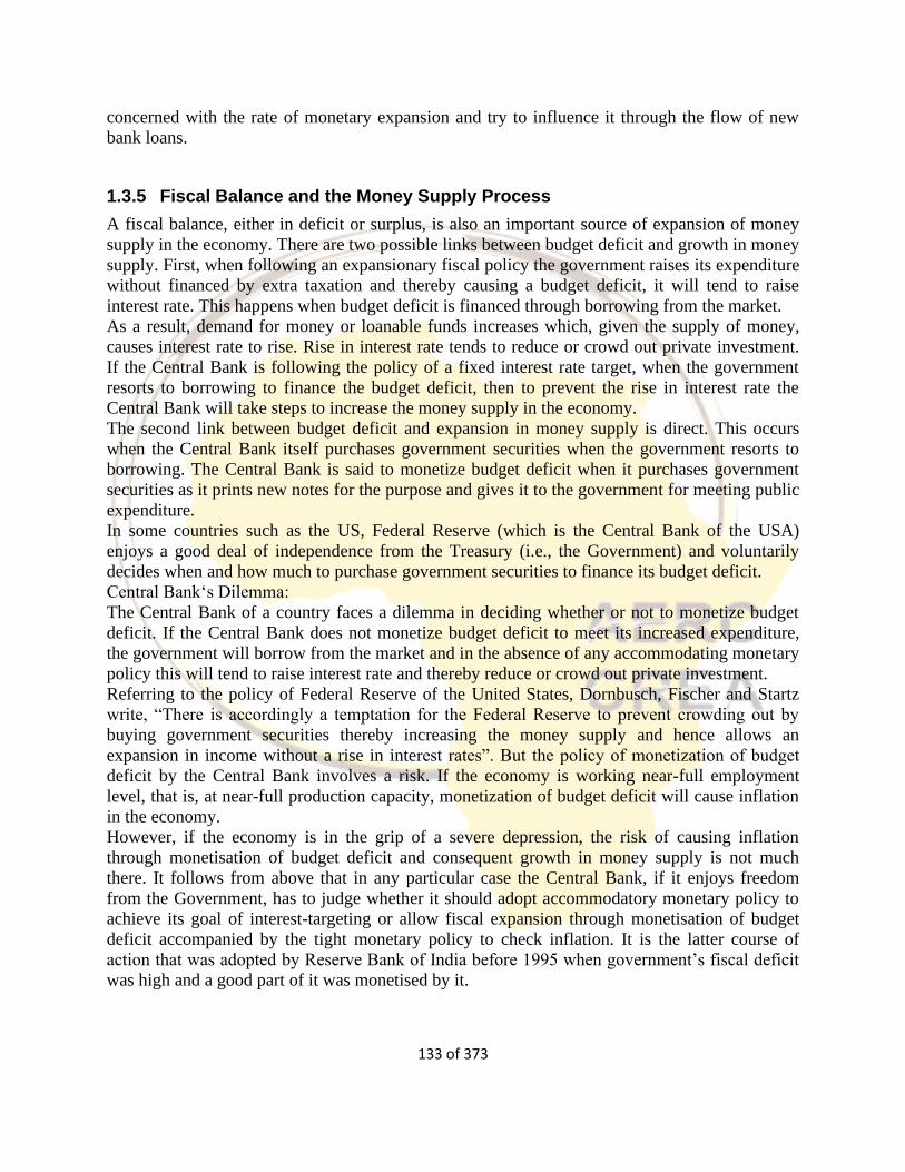
133 of 373

concerned with the rate of monetary expansion and try to influence it through the flow of new

bank loans.

1.3.5 Fiscal Balance and the Money Supply Process

A fiscal balance, either in deficit or surplus, is also an important source of expansion of money

supply in the economy. There are two possible links between budget deficit and growth in money

supply. First, when following an expansionary fiscal policy the government raises its expenditure

without financed by extra taxation and thereby causing a budget deficit, it will tend to raise

interest rate. This happens when budget deficit is financed through borrowing from the market.

As a result, demand for money or loanable funds increases which, given the supply of money,

causes interest rate to rise. Rise in interest rate tends to reduce or crowd out private investment.

If the Central Bank is following the policy of a fixed interest rate target, when the government

resorts to borrowing to finance the budget deficit, then to prevent the rise in interest rate the

Central Bank will take steps to increase the money supply in the economy.

The second link between budget deficit and expansion in money supply is direct. This occurs

when the Central Bank itself purchases government securities when the government resorts to

borrowing. The Central Bank is said to monetize budget deficit when it purchases government

securities as it prints new notes for the purpose and gives it to the government for meeting public

expenditure.

In some countries such as the US, Federal Reserve (which is the Central Bank of the USA)

enjoys a good deal of independence from the Treasury (i.e., the Government) and voluntarily

decides when and how much to purchase government securities to finance its budget deficit.

Central Bank‘s Dilemma:

The Central Bank of a country faces a dilemma in deciding whether or not to monetize budget

deficit. If the Central Bank does not monetize budget deficit to meet its increased expenditure,

the government will borrow from the market and in the absence of any accommodating monetary

policy this will tend to raise interest rate and thereby reduce or crowd out private investment.

Referring to the policy of Federal Reserve of the United States, Dornbusch, Fischer and Startz

write, “There is accordingly a temptation for the Federal Reserve to prevent crowding out by

buying government securities thereby increasing the money supply and hence allows an

expansion in income without a rise in interest rates”. But the policy of monetization of budget

deficit by the Central Bank involves a risk. If the economy is working near-full employment

level, that is, at near-full production capacity, monetization of budget deficit will cause inflation

in the economy.

However, if the economy is in the grip of a severe depression, the risk of causing inflation

through monetisation of budget deficit and consequent growth in money supply is not much

there. It follows from above that in any particular case the Central Bank, if it enjoys freedom

from the Government, has to judge whether it should adopt accommodatory monetary policy to

achieve its goal of interest-targeting or allow fiscal expansion through monetisation of budget

deficit accompanied by the tight monetary policy to check inflation. It is the latter course of

action that was adopted by Reserve Bank of India before 1995 when government’s fiscal deficit

was high and a good part of it was monetised by it.

134 of 373

1.3.6 Empirical Studies of Money Supply

In this section, we review a number of empirical studies on the money supply process using

cointegration and error-corrections techniques, as captured in Handa (2009). We will then

present a detailed empirical case study of money supply in Ghana.

Cointegration and error-correction models of the money supply

There are few cointegration studies on the money supply function and its major components. We

draw the following findings from Baghestani and Mott (1997) to illustrate the nature of empirical

findings on money supply and the problems with estimating this function when monetary policy

shifts.

Baghestani and Mott performed cointegration tests on USA monthly data for three periods,

1971:04 to 1979:09, 1979:10 to 1982:09 and 1983:01 to 1990:06, using the Engle–Granger

techniques. Their variables were log of M1, log of the monetary base (B) and an interest rate

variable (R). The last was measured by the three-month commercial paper rate for the first two

periods and by the differential between this rate and the deposit rate paid on Super NOWs

(Negotiable Orders of Withdrawal at banks) introduced in January 1983. Further, the discount

rate was used as a deterministic trend variable, since it is constant over long periods. The data for

the three periods was separated since the Federal Reserve changed its operating procedures

between these periods.

Baghestani and Mott could not reject the null hypothesis of no cointegration among the

designated variables for 1971:04 to 1979:09. Further, for 1979:10 to 1982:09, while M0 and R

possessed a unit root, M1 did not, so the cointegration technique was not applied for this period.

The only period which satisfied the requirement for cointegration and yielded a cointegration

vector was 1983:01 to 1990:06. The error-correction model was also estimated for this period.

The cointegration between the variables broke down when the period was extended beyond

1990:06. These results have to be treated with great caution. As indicated on money-demand

estimation, cointegration is meant to reveal the long-run relationships and, for reliable results,

requires data over a long period rather than more frequent observations, as in monthly data, over

a few years. The three periods used by Baghestani and Mott were each less than a decade.

For 1983:01 to 1990:06, Baghestani and Mott concluded from their cointegration–ECM results

that the economy’s adjustments to the long-run relationship occurred through changes in the

money supply and the interest rate, rather than in the monetary base. Comparing their findings

across their three periods, we see that changes in the central bank policy regime, such as

targeting monetary aggregates or interest rates, are extremely important in determining the

money supply function in terms of both its coefficients and whether there even exists a long-run

relationship. Further, even regulatory changes such as permitting, after 1980, the payment of

interest on checkable deposits can shift the money-supply function.

CASE STUDY

135 of 373

An Empirical Analysis of the Money Supply Process in Ghana: 1983-20063

Abstract

This paper examines the major drivers of the asset counterpart of the observed money supply in

Ghana since the adoption of the Economic Recovery Programmes in Ghana. Using the

traditional money multiplier approach, the relative contributions of fiscal financing and capital

inflows to the money supply process were examined. It is found that until the mid nineties, fiscal

deficit financing was the major driver of the money supply process. In the later years, however,

changes in the Net Foreign Assets of the Bank of Ghana, driven largely by foreign aid and

remittances inflows, appear to be the major cause of monetary expansion. Until 2003 when

discipline improved, government borrowing was also the major component and source of

changes in the net domestic assets of the BoG. This, the paper argues, implies that the use of

foreign exchange market intervention could be an effective way of controlling money supply.

Theoretical Framework and the Model

The theoretical foundation of the Ghanaian monetary policy strategy, and therefore, of our model

is the standard theory of money supply determination, i.e., the monetary base model. It can be

seen as a simple extension of the traditional bank deposit multiplier approach to deposit creation.

Consider the following balance sheet identity (see Addison, 2001):

M2 = mm2 ×M0 1

Where mm2 is the broad money multiplier, M2 is the broad money supply, and M0 is the

monetary base.The multiplier mm2 is not unique, its components depends on the definition of the

money supply used. However, for brevity, M2 multiplier can be written as:

Where c currency-deposit ratio; r is the reserve ratio; tsfd is the ratio of time, savings and foreign

currency deposit to total deposit ratio.

Assuming that the multiplier can be predicted fairly accurately, or is stable, and then the M2

target can be achieved by setting the corresponding level of M0 through OMO or foreign

exchange reserve management. This is because the monetary base can be decomposed as

follows:

3 Excerpts from Sanusi, A. R, (2010), “An Empirical Analysis of the Money Supply Process in Ghana: 1983-2006”

Journal of Banking and Finance, Vol. 2, No. 1, 2010

136 of 373

where: NFAbog is the net foreign asset of the Bank of Ghana; NDAbog is the net domestic asset

of the Bank of Ghana; NCCGbog is the net credit to central government; NICBPbog is the net

claims on Banks and public; and OINbog is other items (net) of the BoG.

Equation 4 above represents the model. Given the multiplier, it suggests that money supply

expansion can be driven by either rising net foreign asset of the Bank of Ghana, net lending to

the government by the Bank of Ghana, net lending to banks and public. Because these are net

claims on the government, the banks and the public, open market sales have contractionary

effects on NCCG and NICBP, while open market purchases have the opposite effect. Similarly,

sales of foreign currency by the central bank have a contractionary effect on the NFA, while

purchases expand it. Thus, OMO and foreign exchange market intervention can be used through

the balance sheet of the BoG to regulate the level of monetary base and, given the multiplier, the

money supply. However, instability or unpredictability of the multiplier may hinder the

attainment of a desired monetary target.

The model, equations 1 to 4, can also be represented in terms of the rate of growth of the broad

money supply as follows:

In the next section, the model is empirical applied to the pre-inflation targeting period in Ghana.

Empirical Analysis

The Data

In this section, the model estimated using the quarterly data of the Ghana’s monetary survey

obtained from the IMF’s International Financial Statistics for the period 1983Q2-2006Q4. The

choice of this period is informed by the need to cover the post 1983 reform period before the

formal adoption of inflation targeting in December, 2006.

Decomposition of M1 and M2 (Equation 1b)

Figure 1 plots the estimates of Equation 1b, showing changes in real M1, real M0 and the M1

multiplier. It could be observed that the changes in multipliers and monetary base tended to be

somewhat offsetting, as would be expected given some stability in the demand for real money

balances. However, the quarterly fluctuations in both M1 and M2 tend to be associated with net

movements dominated by either the multiplier or the monetary base (Figures 1). Except in a very

few cases, net changes in M0 tend to contribute a relatively higher share of the observed

fluctuations in both aggregates, especially M1 after 1992. In the case of M2, the money

multiplier offset tends to matter more in the later years – a jump in M0 is offset partially by a fall

in the M2 multiplier (Figure 1 panel B)4.

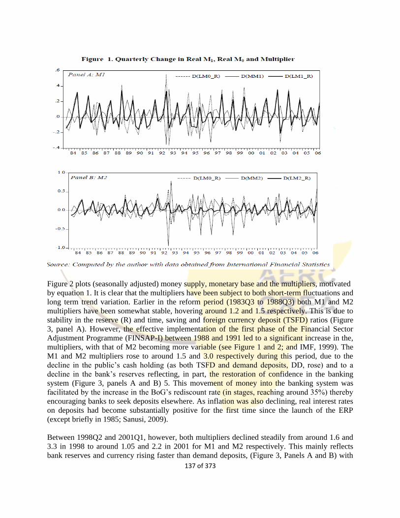
137 of 373

Figure 2 plots (seasonally adjusted) money supply, monetary base and the multipliers, motivated

by equation 1. It is clear that the multipliers have been subject to both short-term fluctuations and

long term trend variation. Earlier in the reform period (1983Q3 to 1988Q3) both M1 and M2

multipliers have been somewhat stable, hovering around 1.2 and 1.5 respectively. This is due to

stability in the reserve (R) and time, saving and foreign currency deposit (TSFD) ratios (Figure

3, panel A). However, the effective implementation of the first phase of the Financial Sector

Adjustment Programme (FINSAP-I) between 1988 and 1991 led to a significant increase in the,

multipliers, with that of M2 becoming more variable (see Figure 1 and 2; and IMF, 1999). The

M1 and M2 multipliers rose to around 1.5 and 3.0 respectively during this period, due to the

decline in the public’s cash holding (as both TSFD and demand deposits, DD, rose) and to a

decline in the bank’s reserves reflecting, in part, the restoration of confidence in the banking

system (Figure 3, panels A and B) 5. This movement of money into the banking system was

facilitated by the increase in the BoG’s rediscount rate (in stages, reaching around 35%) thereby

encouraging banks to seek deposits elsewhere. As inflation was also declining, real interest rates

on deposits had become substantially positive for the first time since the launch of the ERP

(except briefly in 1985; Sanusi, 2009).

Between 1998Q2 and 2001Q1, however, both multipliers declined steadily from around 1.6 and

3.3 in 1998 to around 1.05 and 2.2 in 2001 for M1 and M2 respectively. This mainly reflects

bank reserves and currency rising faster than demand deposits, (Figure 3, Panels A and B) with

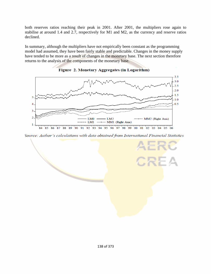
138 of 373

both reserves ratios reaching their peak in 2001. After 2001, the multipliers rose again to

stabilise at around 1.4 and 2.7, respectively for M1 and M2, as the currency and reserve ratios

declined.

In summary, although the multipliers have not empirically been constant as the programming

model had assumed, they have been fairly stable and predictable. Changes in the money supply

have tended to be more as a result of changes in the monetary base. The next section therefore

returns to the analysis of the components of the monetary base.

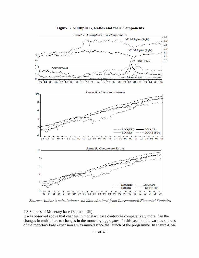
139 of 373

4.3 Sources of Monetary base (Equation 2b)

It was observed above that changes in monetary base contribute comparatively more than the

changes in multipliers to changes in the monetary aggregates. In this section, the various sources

of the monetary base expansion are examined since the launch of the programme. In Figure 4, we

140 of 373

plot equation 2b showing the two components of the changes in monetary base, i.e. ΔNFAbog

and ΔNDAbog. It is noteworthy that over the sample period, the changes in NDA and NFA

tended to be inversely related and, in some quarters, almost offsetting, leading to small or no

change in M0. This is suggestive of the use of one or the other of NDA and NFA for sterilisation

purposes6. For instance, in the early years of the reforms, when foreign exchange inflows were

not a major source of liquidity, the excessive lending to government for deficit financing was

sterilised mainly through the sales of donor supplied foreign exchange (Sowa, 2004)7. The

predominant use of NFA (or foreign exchange intervention) to sterilise expansions in NDA is

reflected in Figure 4 by the tendency of NFA to fall when NDA was rising (negative ΔNFA and

positive ΔNDA), especially up to the end of 1995. The use of foreign exchange intervention

during this period was made easier for at least two reasons: first, the net foreign exchange

inflows were relatively small. Hence, the BoG’s sales of foreign exchange were not generally

enough to satisfy the foreign exchange market, to which it was a major supplier.

Therefore, increased sales of foreign exchange to sterilise NDA expansion could not have

seriously hampered the programmes’ objective of a depreciated cedi. Secondly, given the

shallowness of the financial market, there were few, if any, alternatives to foreign exchange

sterilisation (such as sales of securities).

However, since 1996, the NFA by itself had become a source of liquidity due to the increased

inflows of foreign exchange from foreign aid and external loans for cocoa purchase financing

and remittances. This is reflected in panel B of Figure 4 as increases in M0 are now associated

with increases in NFA (see also the decomposition of equation 2 in Figure A1 in the Appendix).

The BoG, therefore, replaced NDA with M0 as its operational target. The task for the BoG has

since been to control the growth of monetary base (when both NDA and NFA are expanding)

without appreciating the cedi in the process. Accumulation of NFA was therefore used to the

extent that it does not lead to the appreciation of the cedi. The burden of controlling the growth

of M0 was therefore placed generally on limiting NDA. However, as will be shown later,

because

of the persistence of large public sector borrowing requirement (PSBR) that had to be mostly

financed by the BoG, the control of NDA to reduce M0 growth had been initially very difficult8.

As such, many M0 growth targets have been missed as both NFA and NDA grew

simultaneously9. As shown in Figure 4, the reductions in NDA have predominantly been quite

insufficient (and sometime impossible) to offset the increase in NFA10, leading to large

increases

in the M0.

Since 2003 when the BoG was granted de jure independence, the inverse relationship between

NFA and NDA started to appear regular again. This suggests that the BoG during this period has

been better able to achieve reduction in the NDA. As we shall see later, this is partly because of a

reduction in lending to government, and intensive use of OMO as the financial market has

deepened. In the next section, the NDA will be decomposed in order to examine its major

drivers.

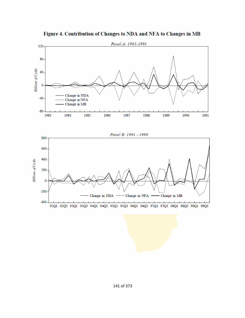
141 of 373

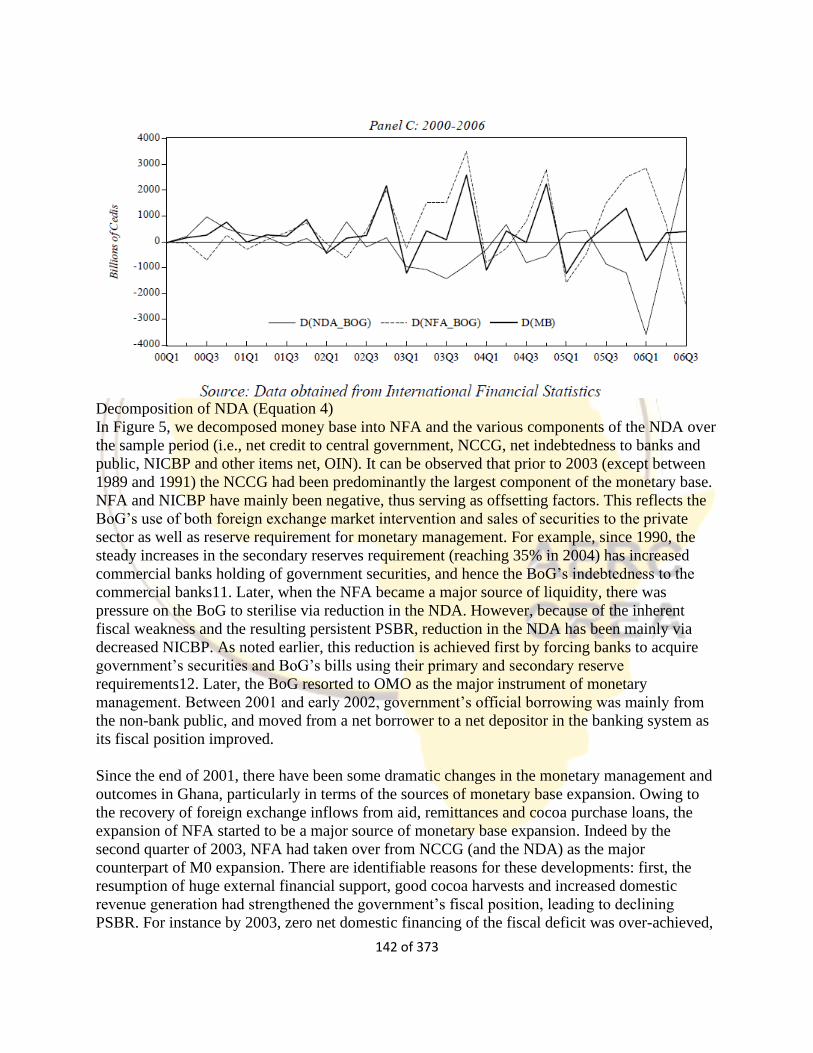
142 of 373

Decomposition of NDA (Equation 4)

In Figure 5, we decomposed money base into NFA and the various components of the NDA over

the sample period (i.e., net credit to central government, NCCG, net indebtedness to banks and

public, NICBP and other items net, OIN). It can be observed that prior to 2003 (except between

1989 and 1991) the NCCG had been predominantly the largest component of the monetary base.

NFA and NICBP have mainly been negative, thus serving as offsetting factors. This reflects the

BoG’s use of both foreign exchange market intervention and sales of securities to the private

sector as well as reserve requirement for monetary management. For example, since 1990, the

steady increases in the secondary reserves requirement (reaching 35% in 2004) has increased

commercial banks holding of government securities, and hence the BoG’s indebtedness to the

commercial banks11. Later, when the NFA became a major source of liquidity, there was

pressure on the BoG to sterilise via reduction in the NDA. However, because of the inherent

fiscal weakness and the resulting persistent PSBR, reduction in the NDA has been mainly via

decreased NICBP. As noted earlier, this reduction is achieved first by forcing banks to acquire

government’s securities and BoG’s bills using their primary and secondary reserve

requirements12. Later, the BoG resorted to OMO as the major instrument of monetary

management. Between 2001 and early 2002, government’s official borrowing was mainly from

the non-bank public, and moved from a net borrower to a net depositor in the banking system as

its fiscal position improved.

Since the end of 2001, there have been some dramatic changes in the monetary management and

outcomes in Ghana, particularly in terms of the sources of monetary base expansion. Owing to

the recovery of foreign exchange inflows from aid, remittances and cocoa purchase loans, the

expansion of NFA started to be a major source of monetary base expansion. Indeed by the

second quarter of 2003, NFA had taken over from NCCG (and the NDA) as the major

counterpart of M0 expansion. There are identifiable reasons for these developments: first, the

resumption of huge external financial support, good cocoa harvests and increased domestic

revenue generation had strengthened the government’s fiscal position, leading to declining

PSBR. For instance by 2003, zero net domestic financing of the fiscal deficit was over-achieved,

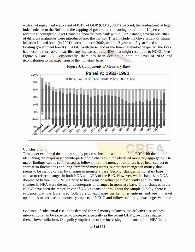
143 of 373

with a net repayment equivalent of 0.4% of GDP (CEPA, 2004). Second, the conferment of legal

independence to the BoG, and the capping of government financing to a limit of 10 percent of its

revenue encouraged budget financing from the non-bank public. For instance, several securities

of different maturities were introduced into the market. These include the Government of Ghana

Inflation Linked bond (in 2001), cocoa bills (in 2002) and the 2-year and 3-year fixed and

floating government bonds (in 2004). With these, and as the financial market deepened, the BoG

had become more able to sterilise any increases in the NDA that might result due to NCCG (see

Figure 5 Panel C). Consequently, there has been decline in both the level of NDA and

itcontribution to the expansion of the monetary base.

Conclusions

This paper examined the money supply process since the adoption of the ERP with the aim of

identifying the major asset counterparts of the changes in the observed monetary aggregates. The

major findings can be summarised as follows: first, the money multipliers have been subject to

short-term fluctuations and long-term trend movements, but the net changes in money shock

seems to be mainly driven by changes in monetary base. Second, changes in monetary base

appear to reflect changes in both NDA and NFA of the BoG. However, while changes in NDA

dominated before 1996, NFA started to have a major influence subsequently and, by 2003,

changes in NFA were the major counterparts of changes in monetary base. Third, changes in the

NCCG have been the major driver of NDA expansion throughout the sample. Finally, there is

evidence that the BoG used both foreign exchange market interventions and open market

operations to sterilise the monetary impacts of NCCG and inflows of foreign exchange. With the

evidence of substantial rise in the demand for real money balances, the effectiveness of these

interventions can be expected to increase, especially as the recent GDP growth is sustained

(hence lower inflation). One policy implication of the increasing dominance of the NFA in the

144 of 373

money supply process is that foreign exchange intervention would be an effective tool of

monetary control.

Discussions and Reviewed Question

The Bank of Ghana provided the following data for a particular year:

Required Reserve Ratio (RRr) = 20%

Excess Reserve Ratio (Er) = 0.25%

Currency Ratio (Cr) = 70%

Money Stock (M) = GH¢25,000 million

Derive the money multiplier, calculate its value given the data above and interpret your results.

Calculate the High Powered Money (H), the level of Banks Deposits, Currency in circulation and

the Total Reserves.

What is the net effect of an increase in the currency ratio (Cr) on the money supply given the

monetary base? Give reasons in support of your answer.

Determine the ratio of banks’ interest yielding assets (loans/securities) to deposits.

In the B-M approach, explain the effects of the following and show them diagrammatically:

a) an introduction of a mandatory reserve ratio in excess of the prudential

ratio currently in force;

b) the development of new deposit liabilities with zero reserve requirements;

c) a dramatic increase in the number and distribution of cash machines.

Using figure 3.1, show the difference in impact on money market equilibrium of a given

reduction in reserve assets when (a) the money supply curve shows some positive elasticity with

respect to the bond rate and (b) when the money supply curve is completely inelastic with respect

to the bond rate.

In the flow of funds analysis, explain the effect of an increase in the government’s budget deficit,

ceteris paribus.

What steps might the authorities take to offset the monetary effects of events in question 4?

Why, according to the flow of funds approach, does the choice of exchange rate regime make

monetary control more, or less, difficult for the authorities?

145 of 373

1.4 MONEY, PRICES AND EMPLOYMENT

Introduction

Welcome to the fourth section of this course where we focus principally on money and inflation

as well as money and employment. The principle that inflation and deflation are fundamentally

monetary phenomena has been one of the best understood and empirically well-founded notions

in monetary economics. Over history, whenever central banks have allowed money growth to

systematically surpass the natural growth of the economy, sooner or later inflation inevitably

followed. Likewise, serious deflationary episodes have invariably been associated with sustained

shortfalls in money growth. Recognition of this fundamental principle over the years has led

many central banks to place special emphasis on reigning in money growth in a continuing effort

to pursue and maintain price stability over time. And consequently, monitoring the growth rate

of money has long been part of the standard monetary practitioner’s toolkit.

In many places around the world, it is by now well understood that the two episodes most

commonly seen as major monetary policy failures since the founding of the Federal Reserve,

namely the Great Depression of the 1930s and the Great Inflation of the 1970s, were episodes

where policymakers failed to properly monitor and heed the warnings present in the behavior of

money. In large part because of these experiences, the Federal Reserve has regularly monitored

the growth of money since the late 1970s.

However, the behavior of monetary aggregates may not always serve as a particularly reliable

guide to inflation. Over shorter horizons, in particular, cyclical developments and transitory

changes in the velocity of money present non-trivial complications. Simple measures of money

growth may not always reliably foreshadow subsequent movements in inflation. From this

perspective, the benefits of close monitoring of the behavior of monetary aggregates as indicators

of inflation over shorter horizons may not always appear very large. The process of constructing

monetary aggregates is inherently an empirical enterprise, fraught with the difficulties of any

such enterprise. Over longer horizons, financial.

In this section, we shall study the various theories propounded to explain the relationship

between money, inflation and employment.

Objectives

By the end of this section you should be able to;

Explain the theoretical links between money and inflation

Explain monetary control and inflation

Describe theories of money growth and business cycles

Explain expectations of the real business cycle and expected inflation

Explain the relationship between money, inflation and employment

146 of 373

1.4.1 Money and Theories of Inflation

Many people have wrong interpretation to what inflation is all about. In this section, we are

going to digest what economists mean when they say inflation. Inflation is a very complex term

which has seen tremendous changes since it was first defined by neo-classical economists. The

neo-classical school of thought initially regarded inflation as a galloping rise in prices as a result

of excessive increase in the supply of money. They regarded inflation “as a destroying disease

born out of lack of monetary control whose results undermined the rules of business, creating

havoc in markets and financial ruin of even the prudent.”

More specifically, the neo-classical school of thought believed that inflation is basically a

monetary phenomenon. Friedman pointed out that, “Inflation is always and everywhere a

monetary phenomenon ……. and can be produced only by a more rapid increase in the quantity

of money than output.” But Hicks noted that , “Our present troubles are not of a monetary

character.” Economists, therefore, define inflation in terms of a continuous rise in prices. For

example whilst Johnson defines “inflation as a sustained rise” in prices, Broman defines it as “a

continuing increase in the general price level. Shapiro in a similar vein defines inflation “as a

persistent and appreciable rise in the general level of prices. Denberg and McDougall however

argued that ‘the term usually refers to a continuing rise in prices as measured by an index such as

the consumer price index (CPI) or by the implicit price deflator for gross national product.’

But Keynes in his General Theory thought otherwise. He was of the view that the economy was

not always at fill employment and so it was not possible for increases in the quantity of money to

result in hyper-inflation. Rather, there is underemployment in the economy, and as such an

increase in the money supply leads to increase in aggregate demand, output and employment.

Starting from a depression, as the money supply increases, output and employment rise further,

diminishing returns start and certain bottlenecks inflation or “semi-inflation” sets in. If the

money supply increases beyond the full employment level, output ceases to rise and prices rise in

proportion with the money supply.

Keynes’ perception of inflation is subjected to two main setbacks. First, it emphasizes on

demand as the major cause of inflation, but neglects the cost side of inflation. Second, it ignores

the possibility that a price rise may lead to further increase in aggregate demand which may, in

turn, lead to further rise in prices. An attempt to provide a working definition for inflation has

rather resulted in a prolonged debate on this subject matter.

I shall try to show that there are only two basic theories of inflation - (l) One is the institutional

theory of inflation and the other (2) one is the money stock theory of inflation. Money stock

theory of inflation considers the Government and the Central Bank to be the generators of

inflation while the institutional theories consider this or that section of the people to be

responsible for inflation. Let us first get familiar with these theories so that our task is henceforth

eased. In what follows we discuss the various theories of inflation.

The Cost-Push Theory of Inflation

The cost-push theory of inflation is the wage push or the profit-push theory of inflation. In every

147 of 373

process of inflation wages and prices rise and they reinforce the rise in each other, whatever the

cause of inflation. But if the cost-push theory is valid, then they both should not be the common

result of some third force which may be a rise in total demand or money supply or what not and

the initiation of inflation should have been made by an autonomous rise in wages or profits.

The main cause of cost-push inflation is wage increases enforced by unions and profit increases

by employers. That is to say that cost-push inflation is caused by wage-push and profit-push to

prices. The primary cause of cost-push inflation is that money wages rise faster than the

productivity of labour. In most countries where trade union activities are effective they are able

to press employers to grant wage increases very much in excess of increases in the productivity

of labour, thereby raising the cost of producing goods and serves. In turn, employers pass on the

increase in the cost of production to consumers in the form of higher prices. Despite the

increase in prices the higher wages enjoyed workers enable to buy as much as before. However,

continuous increase in prices induces unions to make further demands for higher wages. In this

way, the wage-cost spiral continues, thereby leading to cost-push or wage-push inflation.

At certain times the increase in money wages and prices affect a few sectors of the economy.

However products from such sectors are used as inputs for the production of goods and services

in other sectors. Hence the production costs of these other sectors rise and thereby causing the

prices goods produced in these sectors to also rise. Thus wage-push inflation in a few sectors of

the economy may soon be translated into inflationary pressures in the entire economy.

Related closely to the point above is that cost-push inflation can be also be caused by an increase

in the price of domestically produced or imported raw materials. Since raw materials are used as

inputs in the production of finished goods, they affect the cost of production. So then a

continuous rise in the prices of raw materials tend to set off a cost-price-wage spiral.

Cost-push inflation is further caused by profit-push inflation. Oligopolist and monopolist firms

raise the price of their products to offset the rise in labour and production costs so as to earn

higher profits. There being imperfect competition in the case of such firms, they are able to

“administer price” of their products. Profit-push inflation is, therefore, also called administered-

price theory of inflation or price-push inflation or sellers’ inflation or market-power inflation.

Cost-push inflation is illustrated in Figure 4.1 (A) and (B). First consider diagram (B) of the

figure where supply curves represented by the curves SS and SS1 and full employment income

represented by YF. Given the demand conditions as represented by the demand curve D, the

initial supply curve So is shown to shift to S1 in response to cost-increasing pressures from

oligopolies, unions, etc. as a result of rise in money wages. Consequently, the equilibrium

position shifts from E to E1 reflecting rise in the price level from P to P1 and fall in output,

employment and income from Y1 to Y1 level.

In diagram (A) of the figure, as the price level rise, the LM curve shifts to the left to LM,

position because with the increase in the price level to P1 the real value of the money supply

falls. Similarly, the /S curve shifts to the left to IS1 position because with the increase in the

price level the demand for consumer goods falls due to the Pigou effect. Accordingly, the

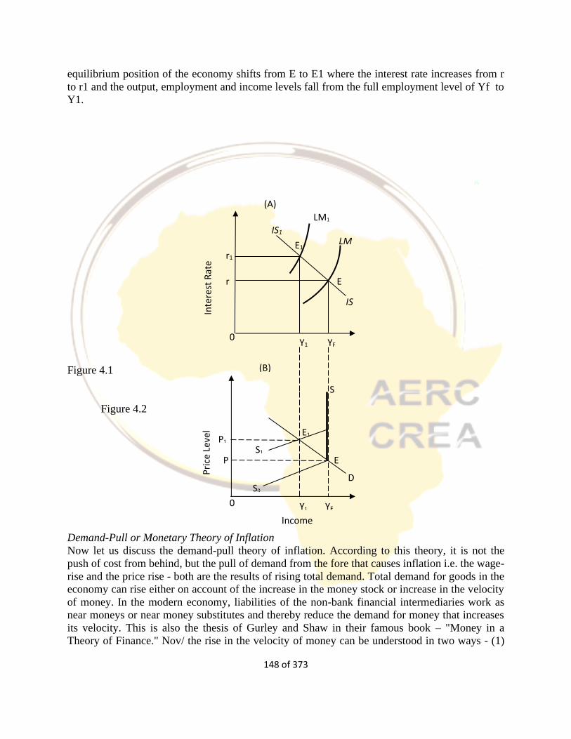
148 of 373

equilibrium position of the economy shifts from E to E1 where the interest rate increases from r

to r1 and the output, employment and income levels fall from the full employment level of Yf to

Y1.

Figure 4.1

Figure 4.2

Demand-Pull or Monetary Theory of Inflation

Now let us discuss the demand-pull theory of inflation. According to this theory, it is not the

push of cost from behind, but the pull of demand from the fore that causes inflation i.e. the wage-

rise and the price rise - both are the results of rising total demand. Total demand for goods in the

economy can rise either on account of the increase in the money stock or increase in the velocity

of money. In the modern economy, liabilities of the non-bank financial intermediaries work as

near moneys or near money substitutes and thereby reduce the demand for money that increases

its velocity. This is also the thesis of Gurley and Shaw in their famous book – "Money in a

Theory of Finance." Nov/ the rise in the velocity of money can be understood in two ways - (1)

Inte

rest

Rat

e

LM

LM1

E1

E

IS

r1

r

YF Y1 0

(A)

Income

0 Y1 YF

E1

S1

D

P1

P

S

S0

E

(B)

Pri

ce L

evel

IS1

149 of 373

firstly, the growth of near money substitutes can lessen the demand for money and thereby can

increase the velocity of money and secondly (2) money held up on account of pervasive controls,

as for example, during war times, may begin to be spent when controls are relaxed or removed,

thereby increasing the turnover of money or the velocity of money.

Demand-pull inflation or excess demand inflation is the most commonly known type of inflation.

It occurs when aggregate demand rises more than the supply of supply of goods and service.

Goods may be in short supply either because resources are not fully utilized or production cannot

be increased quickly to meet the increasing demand. We therefore experience a situation where

“too much money chasing too few goods.”

Two principal theories attempt to explain the demand-pull inflation, namely the Monetarists and

Keynesians theories. We shall also discuss a third one propounded by the Danish economist,

Bent Hansen.

Monetarist View or Monetary Theory of Inflation

Monetarists emphasized the role of money as the principal cause of demand-pull inflation.They

argued that inflation is always a monetary phenomenon. The formal explanation of the

monetarist view was formulated as the simple quantity theory of money and was expressed the

Fisher’s equation of exchange which is of the form:

MV = PQ

where M is the money supply, V is the velocity of money, P is the price level, and Q is the level

of real output.

Assuming V and Q as constant, the price level (P) varies proportionately with the supply of

money (M). With flexible wages, the economy was believed to operate at full employment level.

The labour force, the capital stock, and technology also changed only slowly over time.

Consequently, the amount of money spent did not affect the level of real output so that a

doubling of the quantity of money would result simply in doubling the price level. Until prices

had risen by this proportion, individuals and firms would have excess cash which they would

spend, leading to rise in prices. So inflation proceeds at the same rate at which the money supply

expands. In this analysis the aggregate supply is assumed to be fixed and there is always full

employment in the economy. Naturally, when the money supply increases if creates more

demand for goods but the supply of goods cannot be increased due to the full employment of

resources. This leads to rise in prices. But it is a continuous and prolonged rise in the money

supply that will lead to true inflation.

Friedman the renowned monetary economist however argued that “inflation is always and every

where a monetary phenomenon that arises from a more rapid expansion in the quantity of money

than in total output.” He argues that any time the quantity of money changes nominal income

changes in the same direction. The rise in the general price level and thus inflation arise from the

fact that the increase in income encourages everywhere to increase their demand for goods and

services as they spend their cash balances. For the tact that demand for money is fairly stable,

this excess spending is the outcome of a rise in the nominal quantity of money supplied to the

economy. So inflation is always a monetary phenomenon.

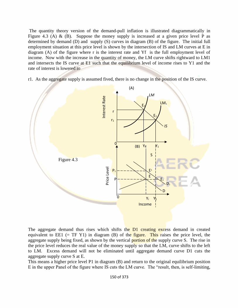
150 of 373

The quantity theory version of the demand-pull inflation is illustrated diagrammatically in

Figure 4.3 (A) & (B). Suppose the money supply is increased at a given price level P as

determined by demand (D) and supply (S) curves in diagram (B) of the figure. The initial full

employment situation at this price level is shown by the intersection of IS and LM curves at E in

diagram (A) of the figure where r is the interest rate and Yf is the full employment level of

income. Now with the increase in the quantity of money, the LM curve shifts rightward to LM1

and intersects the IS curve at E1 such that the equilibrium level of income rises to Y1 and the

rate of interest is lowered to

r1. As the aggregate supply is assumed fived, there is no change in the position of the IS curve.

Figure 4.3

The aggregate demand thus rises which shifts the D1 creating excess demand in created

equivalent to EE1 (= TF Y1) in diagram (B) of the figure. This raises the price level, the

aggregate supply being fixed, as shown by the vertical portion of the supply curve S. The rise in

the price level reduces the real value of the money supply so that the LM, curve shifts to the left

to LM. Excess demand will not be eliminated until aggregate demand curve D1 cuts the

aggregate supply curve S at E.

This means a higher price level P1 in diagram (B) and return to the original equilibrium position

E in the upper Panel of the figure where IS cuts the LM curve. The “result, then, is self-limiting,

LM

LM1 E1

E1

IS

r1

r

YF Y1 0

(A)

Income

0 Yf Y1

E1 D1

D

P1

P

S

E1

E

(B)

Pri

ce L

evel

In

tere

st R

ate

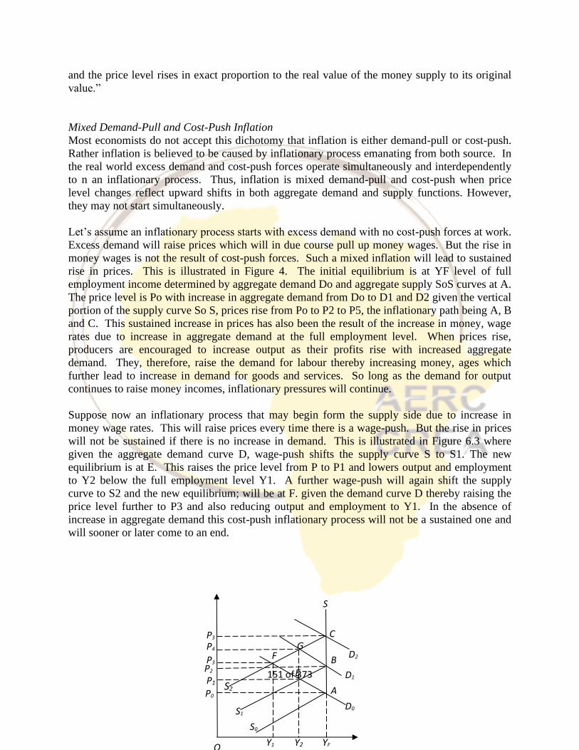
151 of 373

and the price level rises in exact proportion to the real value of the money supply to its original

value.”

Mixed Demand-Pull and Cost-Push Inflation

Most economists do not accept this dichotomy that inflation is either demand-pull or cost-push.

Rather inflation is believed to be caused by inflationary process emanating from both source. In

the real world excess demand and cost-push forces operate simultaneously and interdependently

to n an inflationary process. Thus, inflation is mixed demand-pull and cost-push when price

level changes reflect upward shifts in both aggregate demand and supply functions. However,

they may not start simultaneously.

Let’s assume an inflationary process starts with excess demand with no cost-push forces at work.

Excess demand will raise prices which will in due course pull up money wages. But the rise in

money wages is not the result of cost-push forces. Such a mixed inflation will lead to sustained

rise in prices. This is illustrated in Figure 4. The initial equilibrium is at YF level of full

employment income determined by aggregate demand Do and aggregate supply SoS curves at A.

The price level is Po with increase in aggregate demand from Do to D1 and D2 given the vertical

portion of the supply curve So S, prices rise from Po to P2 to P5, the inflationary path being A, B

and C. This sustained increase in prices has also been the result of the increase in money, wage

rates due to increase in aggregate demand at the full employment level. When prices rise,

producers are encouraged to increase output as their profits rise with increased aggregate

demand. They, therefore, raise the demand for labour thereby increasing money, ages which

further lead to increase in demand for goods and services. So long as the demand for output

continues to raise money incomes, inflationary pressures will continue.

Suppose now an inflationary process that may begin form the supply side due to increase in

money wage rates. This will raise prices every time there is a wage-push. But the rise in prices

will not be sustained if there is no increase in demand. This is illustrated in Figure 6.3 where

given the aggregate demand curve D, wage-push shifts the supply curve S to S1. The new

equilibrium is at E. This raises the price level from P to P1 and lowers output and employment

to Y2 below the full employment level Y1. A further wage-push will again shift the supply

curve to S2 and the new equilibrium; will be at F. given the demand curve D thereby raising the

price level further to P3 and also reducing output and employment to Y1. In the absence of

increase in aggregate demand this cost-push inflationary process will not be a sustained one and

will sooner or later come to an end.

S

C

D2 G

B

D1

A

D0

F

E

S2

S1

S0

Y1 Y2 YF

P3 P4

P3 P2 P1 P0

O

152 of 373

The cost-push inflationary process will be self-sustaining only if every wage-push is

accompanied by a corresponding increase in aggregate demand. Since every cost-push in

accompanied by a fall in output and employment along with a price increase, it is likely that the

government will adopt expansionary monetary and fiscal policies in order to check the fall in

output and employment. In this way, cost-push will lead to a sustained inflationary process

because the government will try to achieve full employment by raising aggregate demand which

will, in turn, lead to further wage-push and so on.

Such a situation is again explained with the help of Figure 6. 3. Suppose there is a wage-push at

E which shifts the supply curve from S1 to S2 and equilibrium is established at F with the

demand curve D0. The price level rises to P3 and the level of employment is reduced to Y1.

When due to an expansionary monetary and fiscal policy, aggregate demand increases to D1, the

new equilibrium position is at G where the price level rises to P4 and the level of employment

rises to Y2. A further increase in demand shifts the aggregate demand curve upward to D2, such

that equilibrium is attained at point C where the price level rises to P2 and the economy attains

the full employment level YF. Thus a wage-push accompanied by an increase in aggregate

demand through expansionary monetary and fiscal policies traces out a ratchet-like inflationary

path from A to E to F to G and to C.

Other Schools of thought on inflation

Keynesian Theory on Inflation

Keynesian theory of inflation works through the investment-saving mechanism. It is little

surprising to note that there are two Keynesian theories of inflation one is demand-pull theory

and the other is the cost-push theory. It may be said that the demand-pull theory was expressed in

the form of an ’inflationary gap* by Keynes in his book "How to Pay for War1’ (J .Pi.Keynes,

1940) and the cost-push theory was contained in his "General Theory."

Keynesians and believers in the quantity theory of money (implicitly or explicitly) are one in the

belief that the immediate cause of inflation is excess demand, though they may disagree

regarding the proximate and the ultimate causes of excess demand itself.

Keynes did not emphasize the excess money supply as the cause of excess demand, because in

U.S.A. during Great Depression, it was widely believed that the Federal Reserve System was

expanding the money supply through the activation of monetary policy and still the economy

was not responding and the effective demand was not reviving. So he felt that the monetary

policy cannot deliver the goods and hence he advocated that the fiscal policy should he activated

and the Government should increase public expenditure and reduce taxes thereby ushering into

budget deficits. Budget deficit implied the expansion of money supply, but he did not emphasize

the growth in money supply which may take the place of hoarded inactive money and thus may

help in reviving demand. He forced money and the monetary policy to take a backseat and put

the fiscal policy in the forefront. He argued that the balancing of the economy was more

important than the

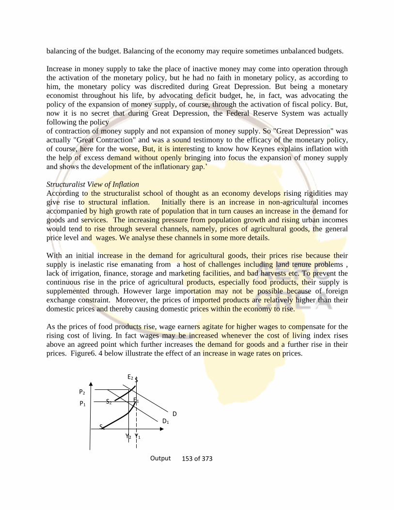
153 of 373

balancing of the budget. Balancing of the economy may require sometimes unbalanced budgets.

Increase in money supply to take the place of inactive money may come into operation through

the activation of the monetary policy, but he had no faith in monetary policy, as according to

him, the monetary policy was discredited during Great Depression. But being a monetary

economist throughout his life, by advocating deficit budget, he, in fact, was advocating the

policy of the expansion of money supply, of course, through the activation of fiscal policy. But,

now it is no secret that during Great Depression, the Federal Reserve System was actually

following the policy

of contraction of money supply and not expansion of money supply. So "Great Depression" was

actually "Great Contraction" and was a sound testimony to the efficacy of the monetary policy,

of course, here for the worse, But, it is interesting to know how Keynes explains inflation with

the help of excess demand without openly bringing into focus the expansion of money supply

and shows the development of the inflationary gap.’

Structuralist View of Inflation

According to the structuralist school of thought as an economy develops rising rigidities may

give rise to structural inflation. Initially there is an increase in non-agricultural incomes

accompanied by high growth rate of population that in turn causes an increase in the demand for

goods and services. The increasing pressure from population growth and rising urban incomes

would tend to rise through several channels, namely, prices of agricultural goods, the general

price level and wages. We analyse these channels in some more details.

With an initial increase in the demand for agricultural goods, their prices rise because their

supply is inelastic rise emanating from a host of challenges including land tenure problems ,

lack of irrigation, finance, storage and marketing facilities, and bad harvests etc. To prevent the

continuous rise in the price of agricultural products, especially food products, their supply is

supplemented through. However large importation may not be possible because of foreign

exchange constraint. Moreover, the prices of imported products are relatively higher than their

domestic prices and thereby causing domestic prices within the economy to rise.

As the prices of food products rise, wage earners agitate for higher wages to compensate for the

rising cost of living. In fact wages may be increased whenever the cost of living index rises

above an agreed point which further increases the demand for goods and a further rise in their

prices. Figure6. 4 below illustrate the effect of an increase in wage rates on prices.

S E2

S2 E1

D

2 D1

Y2 Y1

Output

S1

P2

P1

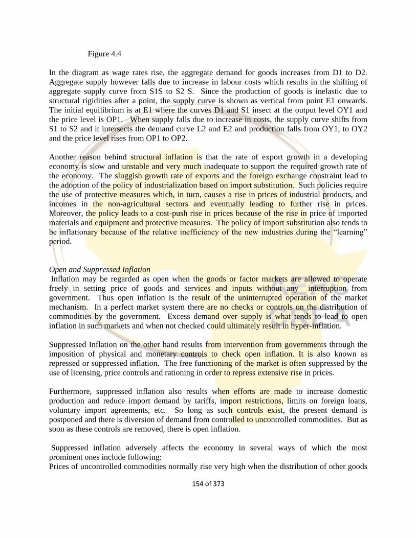
154 of 373

Figure 4.4

In the diagram as wage rates rise, the aggregate demand for goods increases from D1 to D2.

Aggregate supply however falls due to increase in labour costs which results in the shifting of

aggregate supply curve from S1S to S2 S. Since the production of goods is inelastic due to

structural rigidities after a point, the supply curve is shown as vertical from point E1 onwards.

The initial equilibrium is at E1 where the curves D1 and S1 insect at the output level OY1 and

the price level is OP1. When supply falls due to increase in costs, the supply curve shifts from

S1 to S2 and it intersects the demand curve L2 and E2 and production falls from OY1, to OY2

and the price level rises from OP1 to OP2.

Another reason behind structural inflation is that the rate of export growth in a developing

economy is slow and unstable and very much inadequate to support the required growth rate of

the economy. The sluggish growth rate of exports and the foreign exchange constraint lead to

the adoption of the policy of industrialization based on import substitution. Such policies require

the use of protective measures which, in turn, causes a rise in prices of industrial products, and

incomes in the non-agricultural sectors and eventually leading to further rise in prices.

Moreover, the policy leads to a cost-push rise in prices because of the rise in price of imported

materials and equipment and protective measures. The policy of import substitution also tends to

be inflationary because of the relative inefficiency of the new industries during the “learning”

period.

Open and Suppressed Inflation

Inflation may be regarded as open when the goods or factor markets are allowed to operate

freely in setting price of goods and services and inputs without any interruption from

government. Thus open inflation is the result of the uninterrupted operation of the market

mechanism. In a perfect market system there are no checks or controls on the distribution of

commodities by the government. Excess demand over supply is what tends to lead to open

inflation in such markets and when not checked could ultimately result in hyper-inflation.

Suppressed Inflation on the other hand results from intervention from governments through the

imposition of physical and monetary controls to check open inflation. It is also known as

repressed or suppressed inflation. The free functioning of the market is often suppressed by the

use of licensing, price controls and rationing in order to repress extensive rise in prices.

Furthermore, suppressed inflation also results when efforts are made to increase domestic

production and reduce import demand by tariffs, import restrictions, limits on foreign loans,

voluntary import agreements, etc. So long as such controls exist, the present demand is

postponed and there is diversion of demand from controlled to uncontrolled commodities. But as

soon as these controls are removed, there is open inflation.

Suppressed inflation adversely affects the economy in several ways of which the most

prominent ones include following:

Prices of uncontrolled commodities normally rise very high when the distribution of other goods

155 of 373

are controlled.

Suppressed inflation tend to reduce the incentive to work as people do not get the goods they

wish to have.

Controlled distribution of goods also leads to misallocation of resources. This results in the

diversion of productive resources from essential sectors needed by the society.

Frictions increase in the labour market when high inflation is associated with higher

unemployment.

Suppressed inflation leads to black marketing, corruption, hoarding and profiteering. It invites

extra-legal powers of control.

1.4.2 Monetary Control and Inflation

The principle that inflation and deflation are fundamentally monetary phenomena has been one

of the best understood and empirically well-founded notions in monetary economics. Over

history, whenever central banks have allowed money growth to systematically surpass the

natural growth of the economy, sooner or later inflation inevitably followed. Likewise, serious

deflationary episodes have invariably been associated with sustained shortfalls in money growth.

Recognition of this fundamental principle over the years has led many central banks to place

special emphasis on reigning in money growth in a continuing effort to pursue and maintain

price stability over time. And consequently, monitoring the growth rate of money has long been

part of the standard monetary practitioner’s toolkit.

In many countries, it is by now well understood that the two episodes most commonly seen as

major monetary policy failures, namely the Great Depression of the 1930s and the Great

Inflation of the 1970s, were episodes where policymakers failed to properly monitor and heed

the warnings present in the behavior of money. In large part because of these experiences, the

Federal Reserve has regularly monitored the growth of money since the late 1970s.

However, the behavior of monetary aggregates may not always serve as a particularly reliable

guide to inflation. Over shorter horizons, in particular, cyclical developments and transitory

changes in the velocity of money present non-trivial complications. Simple measures of money

growth may not always reliably foreshadow subsequent movements in inflation. From this

perspective, the benefits of close monitoring of the behavior of monetary aggregates as indicators

of inflation over shorter horizons may not always appear very large.

Money growth and inflation

Rewriting the equation of exchange in growth terms, approximated by logarithmic differences,

allows restating this identity in terms of money growth and inflation. In this section, we use this

well-known relationship to illustrate in a simple manner the significance of properly accounting

for changes in equilibrium velocity in assessing the usefulness of money growth as an anchor for

inflation.

For notational convenience, we use lowercase letters to denote logarithms, and adopt the

standard notation 𝜋 = ∆𝑝 for inflation and 𝜇 = ∆𝑚 for money growth. Writing the equation of

156 of 373

exchange in logarithmic form, 𝑚 + 𝜈 = 𝑝 + 𝑞, and taking differences gives:

𝜇 + ∆𝜈 = 𝜋 + ∆𝑞 ……………………..1)

As with the equation of exchange, this relationship is an identity and holds for any

horizon over which growth rates are computed. To allow for a more convenient interpretation,

it is useful to decompose the growth of output and growth of velocity into

their long-run equilibrium components and cyclical components. Defining Q* to denote

the natural level of output (potential output), the cyclical component of output growth

can be captured by the growth rate gap, (∆𝑞 − ∆𝑞 ∗). Likewise, the cyclical component

of velocity growth can be captured by the velocity growth gap, (∆𝜈 − ∆𝜈 ∗). By definition,

both of these gaps tend towards zero as the growth rates are computed over longer

horizons.

Equation (6) can be restated in terms of the cyclical and long-run components of

output and velocity growth as follows:

𝜇 + ∆𝜈 ∗ + (∆𝜈 − ∆𝜈 ∗)=.𝜋 + ∆𝑞 ∗+(∆𝑞 − ∆𝑞 ∗)………………………2)

Rearranging terms to express this relationship in terms of inflation yields:

𝜋 = 𝜇 − ∆𝑞 ∗ +∆𝜈 ∗ − (∆𝑞 − ∆𝑞 ∗) + (∆𝜈 − ∆𝜈 ∗)……………………………..3)

This equation suggests a convenient decomposition of inflation into a cyclical component

and a component determined by money growth adjusted both for the natural

growth of output and changes in equilibrium velocity. Let m* reflect this adjusted money

growth:

𝜇 ∗≡ 𝜇 − ∆𝑞 ∗ +∆𝜈 ∗)………………………………………..4)

Collecting the two cyclical terms

𝜂 = −(∆𝑞 − ∆𝑞 ∗) + (∆𝜈 − ∆𝜈 ∗)……………………………………….5)

And rewriting the equation, yields

𝜋 = 𝜇 ∗ +𝜂 …………………………………….6)

As this equation makes obvious, apart from cyclical effects that tend towards zero over medium-

and long-term horizons, inflation should track adjusted money growth closely. Equation (6), of

course, is simply a restatement of a relationship that is both fundamental and well understood. If

the central bank’s long-run objective is to achieve and maintain inflation at a low and stable

157 of 373

level, 𝜋 *, then this relationship indicates that the central bank must ensure that money growth is

set such that 𝜋 ∗= 𝜇 ∗, over time.

The relationship embedded in equation (6) has served as the basis for determining reference and

monitoring values for the growth of monetary aggregates for a long time. Milton Friedman’s

famous prescription during the late 1960s and early 1970s that monetary policy in the United

States should aim to keep the growth rate of M2 stable at four percent serves as an example. His

prescription was based on the observation that equilibrium M2 velocity appeared to be close to a

constant and the consensus view at the time that the natural growth rate of output was four

percent.

The prescription suggested that abstracting from cyclical effects, stable M2 growth at a four

percent level would achieve near price stability. Another example is the monetary framework

adopted by the Bundesbank from the mid 1970s until the 1990s.

Although the relationship between inflation and money growth in equation (10) follows from an

identity and should be beyond dispute, it is not always sufficiently appreciated. There are at least

two reasons for this confusion. First, over short horizons, this relationship is in large part

overshadowed by cyclical factors. Second, without the proper adjustment for changes in Q* and

V*, money growth and inflation may not appear to track each other even over medium-run

horizons. We illustrate each of these difficulties in turn.

The obvious pitfall here, of course, comes from the fact that the most useful piece of information

provided by money growth regards lower frequency movements in inflation so that any

detrending of the series removes a crucial piece of information from the analysis. Although it is

not uncommon in practice, detrending of inflation may be a seriously flawed procedure in

disentangling the relationship between monetary aggregates and inflation. In short, failing to

properly adjust for

underlying movements in natural growth or equilibrium velocity may obscure the fundamental

link between money growth and inflation but does not in any sense reduce its significance and

value for monitoring inflation.

Empirical Evidence of a Money-Inflation Link

Milton Friedman claimed that “inflation is always and everywhere a monetary phenomenon. “A

Monetary History of the United States, 1867–1960. We know this isn’t true if one takes a loose

view of inflation because negative aggregate supply shocks and increases in aggregate demand

due to fiscal stimulus can also cause the price level to increase. Large, sustained increases in the

price level, however, are indeed proximately caused by increases in the money supply and only

by increases in the money supply. The evidence for this is overwhelming: all periods of

hyperinflation from the American and French Revolutions to the German hyperinflation

following World War I, to more recent episodes in Latin America and Zimbabwe, have been

accompanied by high rates of money supply (MS) growth. In most of those instances, the

government printed money in order to finance large budget deficits.

The rebel American, French, and Confederate (Southern) governments could not raise enough in

taxes or by borrowing to fund their wars, the Germans could not pay off the heavy reparations

imposed on them after World War I, and so forth. We know that the deficits themselves did not

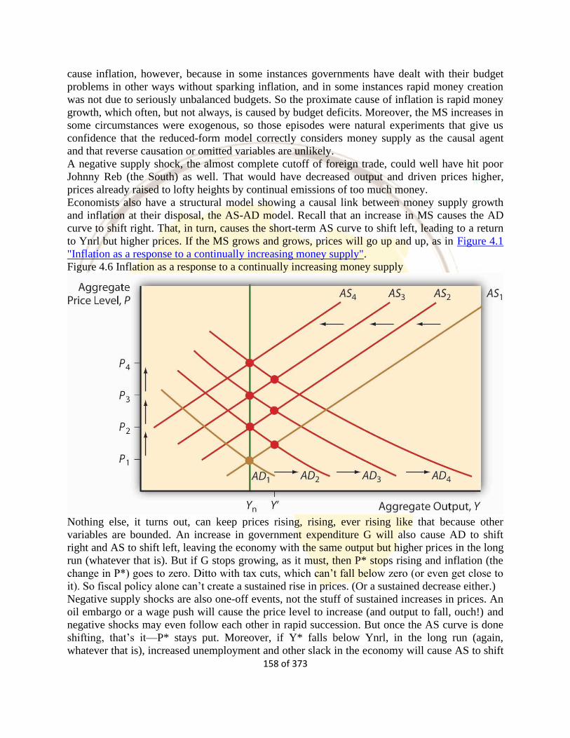
158 of 373

cause inflation, however, because in some instances governments have dealt with their budget

problems in other ways without sparking inflation, and in some instances rapid money creation

was not due to seriously unbalanced budgets. So the proximate cause of inflation is rapid money

growth, which often, but not always, is caused by budget deficits. Moreover, the MS increases in

some circumstances were exogenous, so those episodes were natural experiments that give us

confidence that the reduced-form model correctly considers money supply as the causal agent

and that reverse causation or omitted variables are unlikely.

A negative supply shock, the almost complete cutoff of foreign trade, could well have hit poor

Johnny Reb (the South) as well. That would have decreased output and driven prices higher,

prices already raised to lofty heights by continual emissions of too much money.

Economists also have a structural model showing a causal link between money supply growth

and inflation at their disposal, the AS-AD model. Recall that an increase in MS causes the AD

curve to shift right. That, in turn, causes the short-term AS curve to shift left, leading to a return

to Ynrl but higher prices. If the MS grows and grows, prices will go up and up, as in Figure 4.1

"Inflation as a response to a continually increasing money supply".

Figure 4.6 Inflation as a response to a continually increasing money supply

Nothing else, it turns out, can keep prices rising, rising, ever rising like that because other

variables are bounded. An increase in government expenditure G will also cause AD to shift

right and AS to shift left, leaving the economy with the same output but higher prices in the long

run (whatever that is). But if G stops growing, as it must, then P* stops rising and inflation (the

change in P*) goes to zero. Ditto with tax cuts, which can’t fall below zero (or even get close to

it). So fiscal policy alone can’t create a sustained rise in prices. (Or a sustained decrease either.)

Negative supply shocks are also one-off events, not the stuff of sustained increases in prices. An

oil embargo or a wage push will cause the price level to increase (and output to fall, ouch!) and

negative shocks may even follow each other in rapid succession. But once the AS curve is done

shifting, that’s it—P* stays put. Moreover, if Y* falls below Ynrl, in the long run (again,

whatever that is), increased unemployment and other slack in the economy will cause AS to shift

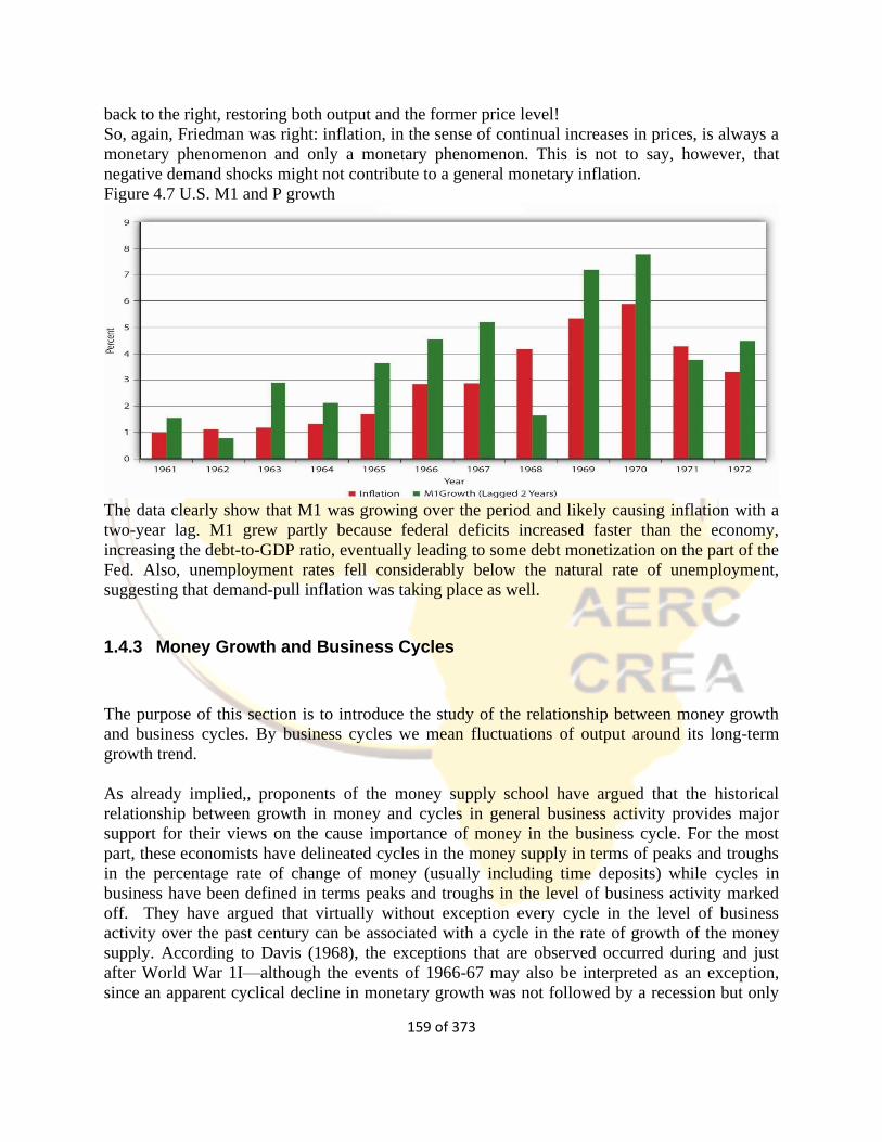
159 of 373

back to the right, restoring both output and the former price level!

So, again, Friedman was right: inflation, in the sense of continual increases in prices, is always a

monetary phenomenon and only a monetary phenomenon. This is not to say, however, that

negative demand shocks might not contribute to a general monetary inflation.

Figure 4.7 U.S. M1 and P growth

The data clearly show that M1 was growing over the period and likely causing inflation with a

two-year lag. M1 grew partly because federal deficits increased faster than the economy,

increasing the debt-to-GDP ratio, eventually leading to some debt monetization on the part of the

Fed. Also, unemployment rates fell considerably below the natural rate of unemployment,

suggesting that demand-pull inflation was taking place as well.

1.4.3 Money Growth and Business Cycles

The purpose of this section is to introduce the study of the relationship between money growth

and business cycles. By business cycles we mean fluctuations of output around its long-term

growth trend.

As already implied,, proponents of the money supply school have argued that the historical

relationship between growth in money and cycles in general business activity provides major

support for their views on the cause importance of money in the business cycle. For the most

part, these economists have delineated cycles in the money supply in terms of peaks and troughs

in the percentage rate of change of money (usually including time deposits) while cycles in

business have been defined in terms peaks and troughs in the level of business activity marked

off. They have argued that virtually without exception every cycle in the level of business

activity over the past century can be associated with a cycle in the rate of growth of the money

supply. According to Davis (1968), the exceptions that are observed occurred during and just

after World War 1I—although the events of 1966-67 may also be interpreted as an exception,

since an apparent cyclical decline in monetary growth was not followed by a recession but only

160 of 373

by a very brief slowdown in the rate of business expansion.' The money supply school also finds

that cycles in business activity have lagged behind the corresponding cycles in the rate of growth

of the money supply, with business peaks and troughs thus following peaks and troughs in the

rate of monetary change. While the evidence supporting these generalizations is derived from

about a century of United States data, the nature of the measurements and some of the problems

The significance, if any, of these leads in assessing the • importance of cycles in money in

causing cycles in business is highly problematical. In support of this, Davis (1968) puts out the

following points: Firstly, chronological leads do not, of course, necessarily imply causation. It is

perfectly possible, for example, to construct models of the economy in which money has no

influence on business but which generate a consistent lead of peaks and troughs in the rate of

growth of the money supply relative to peaks and troughs in general business activity. Secondly,

the extreme variability of the length of the leads would seem to suggest, if anything, (he

existence of factors other than money that can also exert an important influence on the timing of

business peaks and troughs. Certainly even if a peak or trough in the rate of growth of the money

supply could be identified around the time it occurred, this would be of very little, if any, help in

predicting the timing of a subsequent peak or trough in business activity. Thirdly, there is in real

question as to whether anything at all can be inferred from the historical record about the

influence of money on business if, as is argued in the next section, there is an important reverse

influence exerted by the business cycle on the monetary cycle itself.

Let’s now discuss some historical theories about the relationship between Money and business

cycle

An old monetary theory of business cycles was put forward by Hawtrey4. His monetary theory

of business cycles relates to the economy which is under gold standard. It will be remembered

that economy is said be under gold standard when either money in circulation consists of gold

coins or when paper notes are fully backed by gold reserves in the banking system.According to

Hawtrey, increases in the quantity of money raises the availability of bank credit for investment.

Thus, by increasing the supply of credit expansion in money supply causes rate of interest to fall.

The lower rate of interest induces businessmen to borrow more for investment in capital goods

and also for investment in keeping more inventories of goods.

Hawtrey, regards trade cycle as a purely monetary phenomenon. According to him, non-

monetary factors like wars, strikes, earthquakes, crop failures, etc., may cause partial and

temporary depression in particular sectors of the economy, but they cannot cause a full

permanent depression involving general unemployment of the factors of production in the form

of a business cycle. Business cycles are caused by the expansion and contraction of bank credit.

Hawtrey’s business cycle theory is based on three important factors:

1. Traders play an important role in the economy. They are very sensitive to the change of

rate of interest.

2. Money supply in the economy is affected by the level of consumer spending.

3. At the sudden crash of boom, banks suspend credit and call on the borrowers to return the

4 Purely Monetary Theory of Trade Cycle: by Ralph.G. Hawtrey (1926): (1879-1971

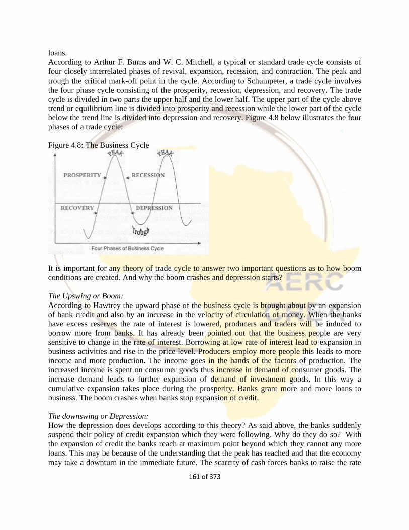
161 of 373

loans.

According to Arthur F. Burns and W. C. Mitchell, a typical or standard trade cycle consists of

four closely interrelated phases of revival, expansion, recession, and contraction. The peak and

trough the critical mark-off point in the cycle. According to Schumpeter, a trade cycle involves

the four phase cycle consisting of the prosperity, recession, depression, and recovery. The trade

cycle is divided in two parts the upper half and the lower half. The upper part of the cycle above

trend or equilibrium line is divided into prosperity and recession while the lower part of the cycle

below the trend line is divided into depression and recovery. Figure 4.8 below illustrates the four

phases of a trade cycle:

Figure 4.8: The Business Cycle

It is important for any theory of trade cycle to answer two important questions as to how boom

conditions are created. And why the boom crashes and depression starts?

The Upswing or Boom:

According to Hawtrey the upward phase of the business cycle is brought about by an expansion

of bank credit and also by an increase in the velocity of circulation of money. When the banks

have excess reserves the rate of interest is lowered, producers and traders will be induced to

borrow more from banks. It has already been pointed out that the business people are very

sensitive to change in the rate of interest. Borrowing at low rate of interest lead to expansion in

business activities and rise in the price level. Producers employ more people this leads to more

income and more production. The income goes in the hands of the factors of production. The

increased income is spent on consumer goods thus increase in demand of consumer goods. The

increase demand leads to further expansion of demand of investment goods. In this way a

cumulative expansion takes place during the prosperity. Banks grant more and more loans to

business. The boom crashes when banks stop expansion of credit.

The downswing or Depression:

How the depression does develops according to this theory? As said above, the banks suddenly

suspend their policy of credit expansion which they were following. Why do they do so? With

the expansion of credit the banks reach at maximum point beyond which they cannot any more

loans. This may be because of the understanding that the peak has reached and that the economy

may take a downturn in the immediate future. The scarcity of cash forces banks to raise the rate

162 of 373

of interest and start withdrawing the short term and call loans from their clients. This comes as

big shock to the businessmen who were enjoying the liberal policy of banks. The sudden call

backs of loans forces businessmen to sell their stock at any price and repay the loans. This

depresses the market. Prices crashes and with every fall in prices the desire to dispose of the

stocks leads to nervousness and collapse of the market.

Once the downtrend starts it gathers the momentum with the lapse of time. There is an

atmosphere of pessimism and gloom throughout the economy. This is depression.

Conditions for revival:

During the depression the rate of interest is low and banks have excess reserves. The conditions

are favourable for revival. The low rate of interest induces businessmen to borrow and the excess

reserves with banks induces banks to lend. The revival starts and because of its cumulative

character leads to prosperity and boom conditions.

In short it can be said that elastic money supply is the root cause of the operation of a trade cycle.

Critical Appraisal:

Hawtrey maintains that the economy under gold standard and fixed exchange rate system makes

his model of business cycles self-generating as there is built-in tendency for the money supply to

change with the emergence of trade deficit and trade surplus which cause movements of gold

between countries and affect money supply in them.

Changes in money supply influence economic activity in a cyclical fashion. However, Hawtrey’s

monetary theory does not apply to the present-day economies which have abandoned gold

standard in 1930s. However, Hawtrey’s theory still retains its importance because it shows how

changes in money supply affect economic activity through changes in price level and rate of

interest. In modern monetary theories of trade cycles this relation between money supply and

rate of interest plays an important role in determining the level of economic activity.

Specific Criticism of the Theory:

1. The theory is criticized for not furnishing a comprehensive explanation of the trade cycle.

2. The rate of interest alone may not affect business decisions.

3. It is also incorrect to say that business fluctuations are caused by the actions of the banks

4. It ignores non-monetary factors, several non-monetary factors, such as new investment

demands, cost structure, and expectations of businessmen, can also produce changes in economic

activities.

5. Hawtrey’s theory that businessmen are more sensitive to the interest rates that is true but

they are influenced by future opportunities to earn profit. Thus bank credit alone cannot explain

the conditions of boom and depression.

Hayek’s Monetary Version:

Hayek suggests that it is monetary forces which cause fluctuations in investment which are prime

cause of business cycles5. In this respect Hayek’s theory is similar to Hawtrey’s monetary theory

5 Friedrich August von Hayek, 1899-1992: Monetary Theory and the Trade Cycle , 1929

163 of 373

except that it does not involve inflow and outflow of gold causing changes in money supply in

the economy.

To begin with, let us assume that the economy is in recession and businessmen’s demand for

bank credit is therefore very low. Thus, lower demand for bank credit in times of recession

pushes down the money rate of interest below the natural rate. This means that businessmen will

be able to borrow funds, that is, bank credit at a rate of interest which is below the expected rate

of return in investment projects. This induces them to invest more by undertaking new

investment projects. In this way, investment expenditure on new capital goods increases.

This causes investment to exceed saving by the amount of newly created bank credit. With the

spurt in investment expenditure, the expansion of the economy begins. Increase in investment

causes income and employment to rise which induces more consumption expenditure. As a

result, production of consumer goods increases. According to Hawtrey, the competition between

capital goods and consumer goods industries for scarce resources causes their prices to rise

which in turn push up the prices of goods and services.

But this process of expansion cannot go on indefinitely because the excess reserves with the

banks come to an end which forces the banks not to give further loans for investment, while

demand for bank credit goes on increasing. Thus, the inelastic supply of credit from the banks

and mounting demand for it because the money rate of interest to go above the natural rate of

interest.

This makes further investment unprofitable. But at this point of time there has been over-

investment in the sense that savings fall short of what is required to finance the desired

investment. When no more bank credit is available for investment, there is decline in investment

which causes both income and consumption to fall and in this way expansion comes to an end

and the economy experiences downswing in economic activity.

However, after a lapse of sometime the fall in demand for bank credit lowers the money rate of

interest which goes below the natural rate of interest. This again gives boost to investment

activity and as a result recession ends. In this way alternating periods of expansion and con-

traction occur periodically.

1.4.4 Expectations of the Real Business Cycle and Expected Inflation

Background: Real Business Cycle (RBC) Theory and Classical Monetary Models

During the years following the seminal papers of Kydland and Prescott (1982) and Prescott

(1986), RBC theory provided the main reference framework for the analysis of economic

fluctuations and became to a large extent the core of macroeconomic theory. The impact of the

RBC revolution had both a methodological and a conceptual dimension. From a methodological

point of view, RBC theory firmly established the use of dynamic stochastic general equilibrium

(DSGE) models as a central tool for macroeconomic analysis. Behavioral equations describing

aggregate variables were thus replaced by first-order conditions of intertemporal problems facing

consumers and firms. Ad hoc assumptions on the formation of expectations gave way to rational

expectations. In addition, RBC economists stressed the importance of the quantitative aspects of

modelling, as reflected in the central role given to the calibration, simulation, and evaluation of

their models. The most striking dimension of the RBC revolution was, however, conceptual. It

164 of 373

rested on three basic claims:

• The efficiency of business cycles. The bulk of economic fluctuations observed in industrialized

countries could be interpreted as an equilibrium outcome resulting from the economy’s response

to exogenous variations in real forces (most importantly, technology), in an environment

characterized by perfect competition and frictionless markets. According to that view, cyclical

fluctuations did not necessarily signal an inefficient allocation of resources (in fact, the

fluctuations generated by the standard RBC model were fully optimal). That view had an

important corollary: Stabilization policies may not be necessary or desirable, and they could even

be counterproductive. This was in contrast with the conventional interpretation, tracing back to

Keynes (1936), of recessions as periods with an inefficiently low utilization of resources that

could be brought to an end by means of economic policies aimed at expanding aggregate

demand.

• The importance of technology shocks as a source of economic fluctuations.

That claim derived from the ability of the basic RBC model to generate “realistic” fluctuations in

output and other macroeconomic variables, even when variations in total factor productivity—

calibrated to match the properties of the Solow residual—are assumed to be the only exogenous

driving force. Such an interpretation of economic fluctuations was in stark contrast with the

traditional view of technological change as a source of long term growth, unrelated to business

cycles.

• The limited role of monetary factors.

Most important, given the subject of the present monograph, RBC theory sought to explain

economic fluctuations with no reference to monetary factors, even abstracting from the existence

of a monetary sector. Its strong influence among academic researchers notwithstanding, the RBC

approach had a very limited impact (if any) on central banks and other policy institutions. The

latter continued to rely on large-scale macroeconometric models despite the challenges to their

usefulness for policy evaluation (Lucas 1976) or the largely arbitrary identifying restrictions

underlying the estimates of those models (Sims 1980).

The attempts by Cooley and Hansen (1989) and others to introduce a monetary sector in an

otherwise conventional RBC model, while sticking to the assumptions of perfect competition and

fully flexible prices and wages, were not perceived as yielding a framework that was relevant for

policy analysis. The resulting framework, which is referred to as the classical monetary model,

generally predicts neutrality (or near neutrality) of monetary policy with respect to real variables.

That finding is at odds with the widely held belief (certainly among central bankers) in the power

of that policy to influence output and employment developments, at least in the short run. That

belief is underpinned by a large body of empirical work, tracing back to the narrative evidence of

Friedman and Schwartz (1963), up to the more recent work using time series techniques, as

described in Christiano, Eichenbaum, and Evans (1999).

165 of 373

Real business cycle theory and monetary policy

Business cycles are cyclical fluctuations in the economy’s output and employment in real, not

analytical, time. Their explanation relates to the short term, which is a chronological concept of

time, rather than the analytical short run or long run. Real business cycle theory is an offshoot of

the modern classical model and asserts that business fluctuations occur only in response to

shocks to the fundamental determinants of long-run output and employment (e.g. see Prescott,

1986; Christiano and Eichenbaum, 1992; Romer, 1996, Ch. 4). These determinants are

technology, which determines the production function and the demand for inputs, and the supply

of factor inputs. Among the determinants of the latter are preferences, including those on labor

supply, which depends on the labor– leisure choice and the stock of resources. Shifts in the

production function or input supplies alter long-run equilibrium output, as well as being a source

of cyclical fluctuations in output.

The real business cycle theory derives the fundamental determinants of business cycles from the

general macroeconomic models of the classical paradigm. Explicitly, or by omission, real

business cycle theory also holds that shifts in aggregate demand, no matter what their source, do

not cause changes in output and employment and therefore do not cause business cycle

fluctuations. Therefore, changes in consumption, investment, exports, money supply and demand

(or the central bank’s interest rate policy) or fiscal deficits cannot change output and

employment. This exclusionary proposition is derived from the properties of the long-run

equilibrium of the modern classical model. To be valid, it requires perfectly competitive markets

and also that long-run equilibrium is continuously maintained in the economy.

The policy implication of real business cycle theory, as of the modern classical model of which it

is an elaboration, is that systematic monetary (and fiscal) policies cannot affect output and

employment, so that they cannot be used to moderate the business cycle. The critical elements

for this implication are the Friedman–Lucas supply equation and rational expectations, according

to which anticipated changes in prices, inflation and monetary policy cannot affect output.

Therefore, the Taylor rule, under which systematic monetary policy manipulates aggregate

demand by changing the interest rate in response to the output gap and the deviation of inflation

from its target rate, can only be useful in controlling inflation but not in moderating the output

gap. According to the modern classical school, while random monetary policy can change

aggregate demand, the central bank cannot predict and therefore cannot offset the random

fluctuations in the private components of aggregate demand. In short, in the new classical model,

monetary policy and the Taylor rule have no legitimate role in moderating or reducing the

duration of business cycles.

Intuitively, the problem with the real business cycle theory is most evident in its explanation of

recessions. It attributes recessions to a fall in labor productivity and/or an increase in the

preference for leisure. The objections to these explanations are succinctly stated by the quip:

recessions occur because “workers forget how to do things” (“lose some of their knowledge”)

and/or because they decide to become lazier for some time, thereby causing the recessionary fall

in output! Neither of these explanations is plausible, so the validity of the real business cycle

theory is highly doubtful. Looking at upturns in business cycles, the real business cycle theory

attributes upturns to increases in productivity and/or increases in the preference for work over

166 of 373

leisure. The latter is hardly plausible over the length of upturns in the economy, while the former

is highly plausible. Here, however, it is the plausibility of the assertion of real business cycle

theory that aggregate demand increases cannot also be a source of upturns that is highly doubtful.

The real business cycle propositions rest on the assumption that all markets can be taken to be

competitive and efficient (i.e. continuous equilibrium) in the economy. This assumption is not

consistent with models of the Keynesian paradigm, since they incorporate market imperfections

and/or failure of the economy to achieve long-run equilibrium instantly after a demand shock. In

these models, shifts in aggregate demand, whether through shifts in investment and other private

sector variables or in monetary and fiscal policy, can produce changes in output and be a source

of, or contribute to the continuation of, business cycles. More specifically on monetary policy,

market imperfections can create non-neutrality of money, so that fluctuations in the money

supply can add to output fluctuations. Conversely, the appropriate monetary policy can reduce

the severity of cyclical fluctuations due to aggregate demand shocks coming from the private

sector. Further, Keynesians do not deny that shifts in the fundamental determinants of output,

mentioned above, can also cause output fluctuations.

Therefore, the core of the debate about the validity of real business cycle theory is not about

whether shocks to technology and factor inputs can cause cyclical fluctuations, for that is not in

dispute. It is rather about whether shocks to aggregate demand can cause such fluctuations and

whether monetary policy can moderate them. Real business cycles and the modern classical

school deny that they can, or do so in a significant manner, while Keynesians assert that they can

do so. This issue is easily testable by the appropriate causality tests. The consensus on the

empirical evidence seems to be that the major part (in some estimates, as large as 70 percent) of

the fluctuations in output can be attributed to productivity shocks. This is a testament to the

success of real business cycle theory, as compared with Keynesian ideas from the 1940s to the

1970s that had attributed most business cycle fluctuations to shifts in aggregate demand.

However, the empirical evidence leaves a very significant part of the fluctuations in output that

cannot be explained by shifts in technology and preferences. Overall, the empirical evidence, as

well as intuition, seems to indicate that fluctuations in aggregate demand, in addition to changes

in technology and preferences, do cause fluctuations in output and employment and that money

supply growth is positively related to output growth. Therefore, real business cycle theory is not

strictly valid, and monetary policy can be pursued in appropriate cases to reduce output

fluctuations.

The exponents of the real business cycle theory also prefer to test this theory by the calibration

and simulation of models rather than by the econometric testing of their hypotheses. The former

procedure requires a priori specification of the likely values of the parameters, on which there

can be considerable doubts. Further, the findings may not be robust to small changes in these

assumed values, or consistency with the empirical observations may require implausible values.

Consequently, this testing procedure and its reported findings have not won general acceptance.

There seem to be at least two major contributions of the real business cycle theory. One, it has

firmly established that changes in technology and preferences do cause cyclical fluctuations in

167 of 373

output and may do so significantly more than fluctuations in aggregate demand. Two, the

approach initiated by the real business cycle agenda to macroeconomic modeling is now firmly

established. This approach requires that macroeconomics be based on optimization over time by

individual economic agents in a dynamic context. This stochastic dynamic intertemporal

approach to macroeconomics permeates current macroeconomic models, including the new

Keynesian model, which is presented in the next chapter. The major deficiency and unrealistic

assertion of the real business cycle theory is that it denies demand shifts any role in output

fluctuations.

The empirical evidence on the impact of changes in aggregate demand on output is often on the

impact of money supply changes, which change aggregate demand, on output. The influential

study by Friedman and Schwartz (1963a,b) used evidence from over 100 years of US data to

show clear evidence that money supply changes lead, and therefore Granger cause, changes in

real economic activity. However, inside money (i.e. deposits in banks) is the largest component

of money. Subsequent contributions by other authors showed that deposits respond to

macroeconomic disturbances, so that money is more highly correlated with lagged output than

with future output; i.e. deposits lag rather than lead output. However, monetary aggregates such

as M2 still lead output. Further, if the central bank uses the interest rate as its operating monetary

policy target, and money supply responds endogenously to it, the evidence seems to show that

changes in interest rates lead output.

To conclude, empirical evidence shows that while shocks to real factors such as technology and

preferences do cause fluctuations in output, shocks to monetary policy variables of money and

interest rates also do so. Models of the modern classical school and real business cycle theory do

not provide a satisfactory explanation for the latter finding. In recent years, sticky price and

inflation models of the new Keynesian school have been proposed to explain economic

fluctuations. An example of these studies is provided by Ireland (2001b).

1.4.5 Money and Employment

We consider the impact of changes in money stock and interest rates on real income and

employment. However, our ultimate concern is with their effect on real variables and on the rate

of inflation.

Before Keynes’s General Theory, this was the preserve of the Quantity Theory of Money, which

suggested that, in anything other than the short run, any change in the rate of growth of the

money supply would simply lead to inflation. Real income (output) was assumed to be

determined by the real forces of saving (thrift) and productivity and not by monetary factors. As

we have seen, this required a stable demand for money and hence a stable income velocity of

money. There was thus, effectively, no trans- mission mechanism between changes in the money

supply and output. Long run real interest rates could not be influenced by monetary policy.

Classical theory argued that they were determined by the behaviour of savers and investors, as

168 of 373

set out in the loanable funds theory of the determination of interest rates. Both saving and

investment decisions, and hence the real rate of interest, depended on long-term considerations.

The monetary authorities could influence nominal interest rates, but these were of no long-run

significance for the real economy. This picture was disturbed by Keynes’s General Theory and

by the interpretations made by Keynesians of this theory. In this view, the nominal interest rate

was determined by the demand for and supply of money and provided a vital link between the

real and monetary sectors of the economy. Changes in nominal interest rates could bring about

changes in real interest rates and have an effect on the real variables of output and employment.

Further, the demand for money was held not to be stable and hence control of the money supply

would not have a predictable effect on nominal income. The interest rate became the accepted

monetary policy instrument but, monetary policy was thought to have only a weak effect on

nominal income, especially when the economy was in recession.

However, whenever the economy was operating at less than full employment, any impact on

nominal income implied also an impact on output since inadequate demand was argued to be a

major cause of unemployment. This approach explained the standard Keynesian models in which

the general price level was assumed to be constant and hence no distinction was made between

nominal income and output. An increase in demand implied an increase in output and

employment. It was always acknowledged that excess demand would cause prices to increase

when the economy was at full employment as inflationary gaps (the gap between aggregate

demand and aggregate supply at the existing price level) developed. In more detailed models,

prices had to rise before the economy was at full employment because an increase in

employment required a reduction in real wages and this could only occur through an increase in

the general price level. There was thus an inherent notion of a trade-off between reductions in

unemployment and increases in the price level.

Despite this, there was little enquiry into this trade-off until 1958 when A W Phillips first

constructed the Phillips curve (Phillips, 1958). Section 8.2 deals with the original Phillips curve

and the subsequent attack on the idea of the existence of a long-run trade-off between wage

inflation and unemployment in the Friedman-Phelps expectations-augmented Phillips curve.

Unfortunately for the New Classical model, it is clear from the evidence that there is a short-run

trade off between inflation and unemployment. A monetary policy shock does have real effects,

at least in the short-run. Further, the impact of such a shock on unemployment precedes the

impact

on the rate of inflation. The New Classical model had a powerful effect on the way in which

people looked at economic policy. In particular, it led to the policy irrelevance proposition that

the authorities cannot influence real variables by boosting or squeezing aggregate demand.

The simple Phillips curve

After World War II, the UK government accepted for the first time the obligation to try to run

the economy as close to full employment as possible, although the term ‘full employment’ was

never precisely defined. Keynes’s General Theory had suggested that economies in deep

recession could reduce unemployment by expanding aggregate demand and that, in such

circumstances, fiscal policy was likely to provide a more powerful instrument than monetary

policy. There appeared to be empirical support for these ideas. Unemployment had been high in

169 of 373

the 1930s when demand was low; it was non-existent during the war years when demand for

everything outstripped supply; and it seemed in the 1950s that expansionary demand

management could reverse small increases in unemployment.

After 1958, the idea that governments could effectively choose the level of employment and

output up to some critical full employment level, enjoyed what appeared to be overwhelming

empirical support from the work of A W Phillips (1958). The Phillips curve plotted the

relationship in the UK between the recorded level of unemployment (U) and the rate of change

of money wages ( ) from 1861 to 1957. The rate of change of money wages was used as a proxy

for inflation since price inflation data was not available for the early years. Figure 4.4 shows a

simple Phillips curve with wage inflation on the vertical axis. However, it was easy to move

from wage inflation to price inflation by allowing for increases in labour productivity and the

Phillips curve is almost always drawn in price inflation/unemployment space.

The theory of the Phillips curve seemed stable and predictable. Data from the 1960’s modeled

the trade-off between unemployment and inflation fairly well. The Phillips curve offered

potential economic policy outcomes: fiscal and monetary policy could be used to achieve full

employment at the cost of higher price levels, or to lower inflation at the cost of lowered

employment. However, when governments attempted to use the Phillips curve to control

unemployment and inflation, the relationship fell apart. Data from the 1970’s and onward did not

follow the trend of the classic Phillips curve. For many years, both the rate of inflation and the

rate of unemployment were higher than the Phillips curve would have predicted, a phenomenon

known as “stagflation. ” Ultimately, the Phillips curve was proved to be unstable, and therefore,

not usable for policy purposes.

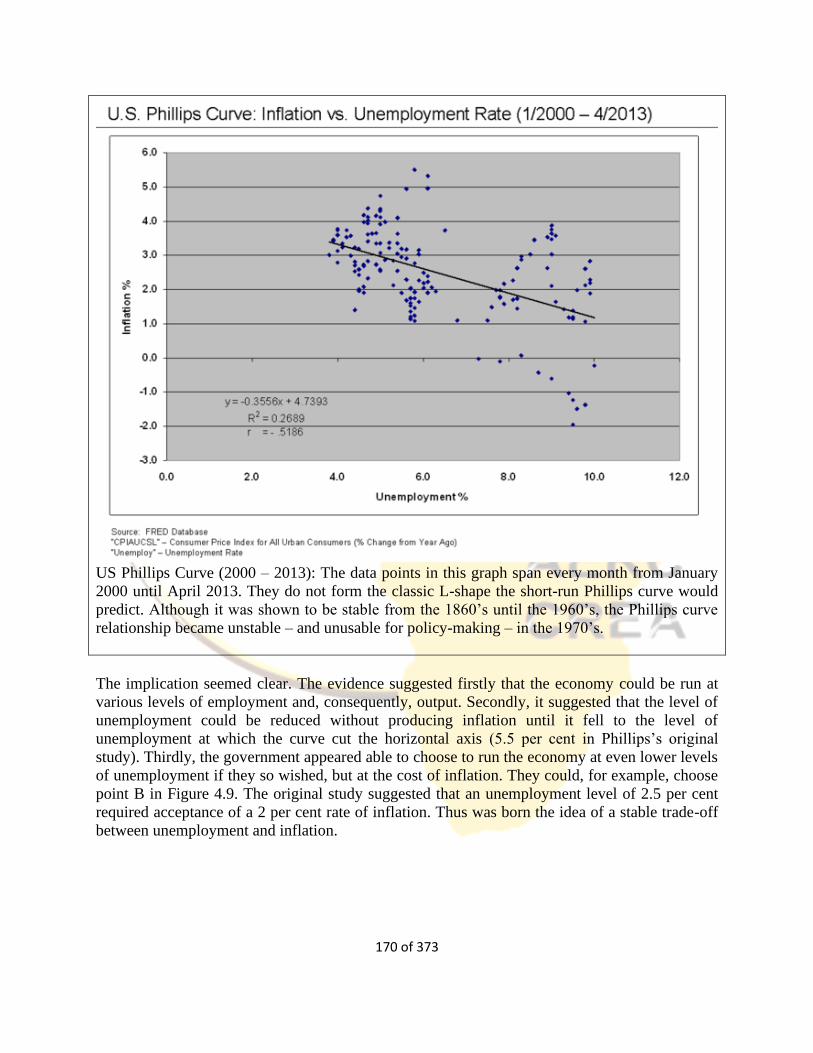
170 of 373

US Phillips Curve (2000 – 2013): The data points in this graph span every month from January

2000 until April 2013. They do not form the classic L-shape the short-run Phillips curve would

predict. Although it was shown to be stable from the 1860’s until the 1960’s, the Phillips curve

relationship became unstable – and unusable for policy-making – in the 1970’s.

The implication seemed clear. The evidence suggested firstly that the economy could be run at

various levels of employment and, consequently, output. Secondly, it suggested that the level of

unemployment could be reduced without producing inflation until it fell to the level of

unemployment at which the curve cut the horizontal axis (5.5 per cent in Phillips’s original

study). Thirdly, the government appeared able to choose to run the economy at even lower levels

of unemployment if they so wished, but at the cost of inflation. They could, for example, choose

point B in Figure 4.9. The original study suggested that an unemployment level of 2.5 per cent

required acceptance of a 2 per cent rate of inflation. Thus was born the idea of a stable trade-off

between unemployment and inflation.

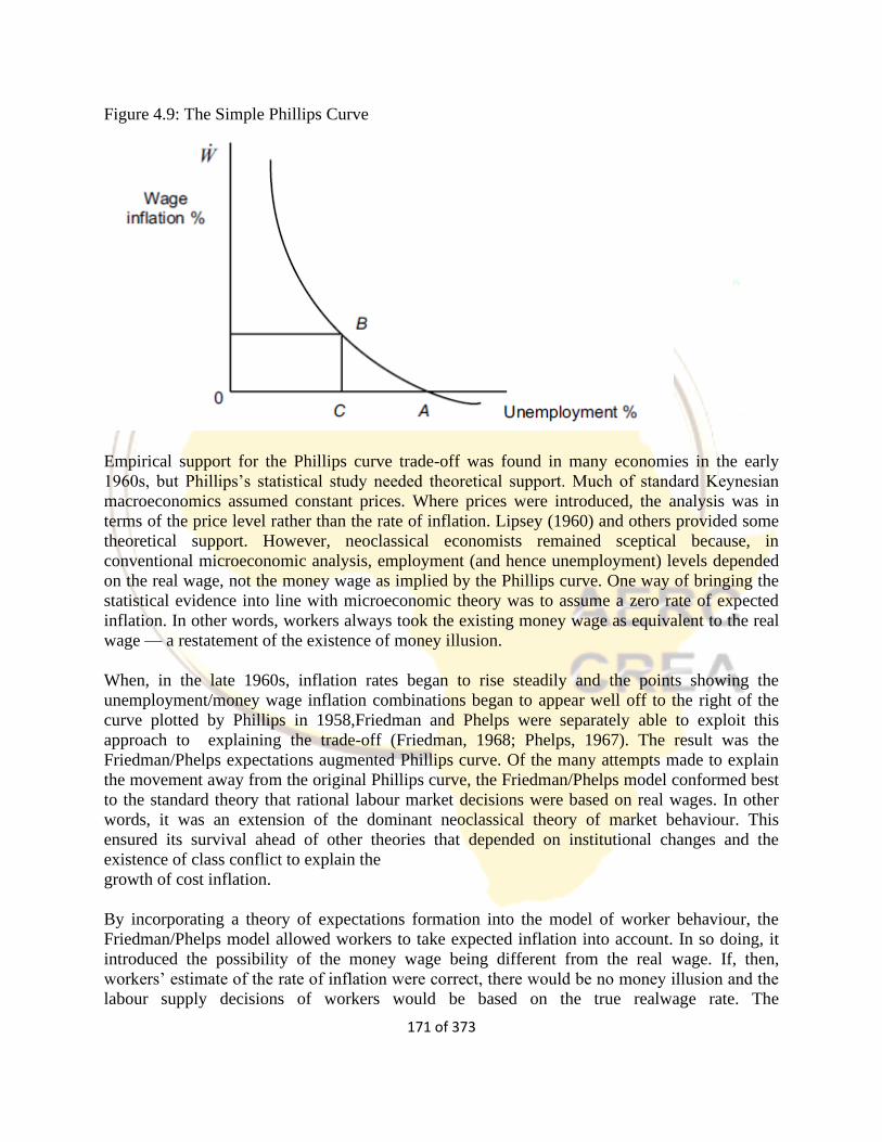
171 of 373

Figure 4.9: The Simple Phillips Curve

Empirical support for the Phillips curve trade-off was found in many economies in the early

1960s, but Phillips’s statistical study needed theoretical support. Much of standard Keynesian

macroeconomics assumed constant prices. Where prices were introduced, the analysis was in

terms of the price level rather than the rate of inflation. Lipsey (1960) and others provided some

theoretical support. However, neoclassical economists remained sceptical because, in

conventional microeconomic analysis, employment (and hence unemployment) levels depended

on the real wage, not the money wage as implied by the Phillips curve. One way of bringing the

statistical evidence into line with microeconomic theory was to assume a zero rate of expected

inflation. In other words, workers always took the existing money wage as equivalent to the real

wage — a restatement of the existence of money illusion.

When, in the late 1960s, inflation rates began to rise steadily and the points showing the

unemployment/money wage inflation combinations began to appear well off to the right of the

curve plotted by Phillips in 1958,Friedman and Phelps were separately able to exploit this

approach to explaining the trade-off (Friedman, 1968; Phelps, 1967). The result was the

Friedman/Phelps expectations augmented Phillips curve. Of the many attempts made to explain

the movement away from the original Phillips curve, the Friedman/Phelps model conformed best

to the standard theory that rational labour market decisions were based on real wages. In other

words, it was an extension of the dominant neoclassical theory of market behaviour. This

ensured its survival ahead of other theories that depended on institutional changes and the

existence of class conflict to explain the

growth of cost inflation.

By incorporating a theory of expectations formation into the model of worker behaviour, the

Friedman/Phelps model allowed workers to take expected inflation into account. In so doing, it

introduced the possibility of the money wage being different from the real wage. If, then,

workers’ estimate of the rate of inflation were correct, there would be no money illusion and the

labour supply decisions of workers would be based on the true realwage rate. The

172 of 373

Friedman/Phelps model assumed the use of adaptive expectations by workers, with workers

basing their expectations of inflation on a weighted average of past inflation rates. Their

expectations are said to be backward looking. This means that past errors are built into future

forecasts (the errors are serially correlated). When inflation is increasing, workers systematically

underestimate the rate of inflation and vice versa. Thus, if inflation were to increase steadily over

a number of years, workers would expect higher and higher inflation rates and would push

money wages up to reflect this.

Consequently, the gap between the money wage rate and the equilibrium real wage rate would

grow — workers would demand higher and higher money wage rates to supply the same quantity

of labour as before. The combinations of unemployment and the rate of inflation experienced by

the economy would appear above and to the right of the curve plotted by Phillips. Thus,

according to Friedman/Phelps, there was a different short run Phillips curve for every expected

rate of inflation. On each such short run curve, there would be one point at which workers’

estimate of the real wage would be correct, and this would be the longrun position. Linking these

long-run positions together provided the vertical long-run ‘Phillips curve’ at the level of

unemployment that existed when the labour market was in equilibrium. This was called the

‘natural rate of unemployment’. It extended the previously existing notion of ‘voluntary’

unemployment resulting from workers placing too high a value upon their leisure by allowing

also for unemployment caused by structural factors (such as the level of economic development

and the characteristics of the labour market). Crucially, however, it did not include

unemployment caused by lack of aggregate demand — at the natural rate of unemployment,

unemployment is balanced by job vacancies. Thus, government could only hope to reduce the

natural rate of unemployment by microeconomic policies that affected the structural

characteristics of markets or the incentives faced by economic agents in making their

work/leisure choices, not by increasing aggregate demand.

The natural rate of unemployment could occur with any rate of inflation and would do so as long

as the expected rate of inflation was equal to the actual rate of inflation. The notion of a long run

trade-off between unemployment and inflation had been completely removed. The rate of

inflation would be explained, as in the Quantity Theory of Money, by the rate of growth of the

money supply. The model, thus, supports the simple rule of monetary policy proposed by Milton

Friedman — that the rate of growth of the money supply in a stable price environment should be

kept equal to the rate of change in real income. Short-run trade-offs between unemployment and

inflation could exist but only because the economy was out of equilibrium. We start at point A in

Figure 4.5, with the rate of inflation having been at zero for some years and with workers

expecting it to remain at zero. We assume, next, that the authorities increase the rate of growth of

the money supply in the hope of reducing unemployment. Inflation unexpectedly increases to

two per cent.

The real wage falls but workers continue to offer labour to the market as if it had not done so. At

the lower real wage rate, employers hire more workers and expand production. Output and

employment increase and we move along the short-run Phillips curve from A to B. However,

workers gradually adapt their expectations to take into account the true rate of inflation and, so

long as the rate of inflation remains at 2 per cent, they will eventually forecast it correctly.

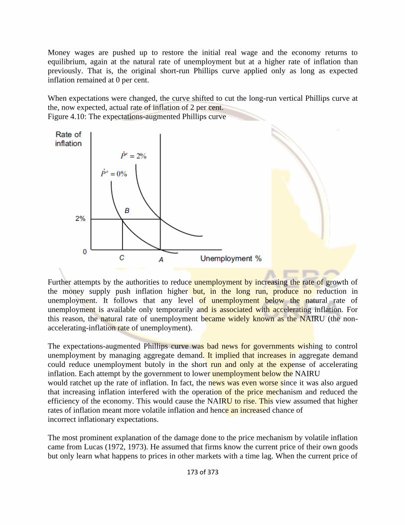
173 of 373

Money wages are pushed up to restore the initial real wage and the economy returns to

equilibrium, again at the natural rate of unemployment but at a higher rate of inflation than

previously. That is, the original short-run Phillips curve applied only as long as expected

inflation remained at 0 per cent.

When expectations were changed, the curve shifted to cut the long-run vertical Phillips curve at

the, now expected, actual rate of inflation of 2 per cent.

Figure 4.10: The expectations-augmented Phillips curve

Further attempts by the authorities to reduce unemployment by increasing the rate of growth of

the money supply push inflation higher but, in the long run, produce no reduction in

unemployment. It follows that any level of unemployment below the natural rate of

unemployment is available only temporarily and is associated with accelerating inflation. For

this reason, the natural rate of unemployment became widely known as the NAIRU (the non-

accelerating-inflation rate of unemployment).

The expectations-augmented Phillips curve was bad news for governments wishing to control

unemployment by managing aggregate demand. It implied that increases in aggregate demand

could reduce unemployment butoly in the short run and only at the expense of accelerating

inflation. Each attempt by the government to lower unemployment below the NAIRU

would ratchet up the rate of inflation. In fact, the news was even worse since it was also argued

that increasing inflation interfered with the operation of the price mechanism and reduced the

efficiency of the economy. This would cause the NAIRU to rise. This view assumed that higher

rates of inflation meant more volatile inflation and hence an increased chance of

incorrect inflationary expectations.

The most prominent explanation of the damage done to the price mechanism by volatile inflation

came from Lucas (1972, 1973). He assumed that firms know the current price of their own goods

but only learn what happens to prices in other markets with a time lag. When the current price of

174 of 373

its output rises, a firm has to decide whether this reflects a real increase in demand for its own

product or a general increase in prices resulting from random demand shocks. In the former

case, the rational response would be to increase its output; in the latter case, it should not do so.

That is, firms have to distinguish between absolute and relative prices. The signal that should be

provided to producers by changes in relative prices is being confused by the possibility of

inflation, especially by volatile inflation. Firms face a signal extraction problem. The greater the

variability of the general price level, the more difficult it is for a producer to extract the correct

signal, and the smaller the supply response is likely to be for any given change in prices. Far

from there being a trade-off between unemployment and inflation, the accepted theory now

suggested that inflation caused unemployment to increase.

To reduce unemployment in the long-run, governments were required to keep inflation low and

to attempt to lower the NAIRU through supply-side measures. There was also bad news for those

authorities who started with a high rate of inflation and wished to get it down. Reducing the rate

of growth of the money supply would push inflation down but workers would continue for some

time to expect the previous high rate of inflation and would continue to push money wages up in

line with their expectations. Real wages would rise, output would fall, and unemployment would

increase beyond the NAIRU. The amount of output lost in order to bring about a fall in inflation

was called the sacrifice ratio. Of course, in the long run, workers would adjust their expectations

and unemployment would fall back to the NAIRU.

However, the short-term costs in terms of lost output and increased unemployment could be

high, especially since the theory did not indicate how long it would take workers to adjust their

expectations. The ‘long run’ is a logical construct —- the time that it takes for workers to obtain

full information about changing prices. However, in a constantly changing world, this could be a

very long time. Indeed, there is no reason to believe that any economy ever reaches the long-run.

Thus, within the Friedman/Phelps model, monetary policy might have considerable and

continuing real effects.

There are other objections to the theory. Firstly, the evidence that inflation was very costly for

economies even at low levels was not strong. The principal loss for an economy identified by

Friedman and others (called the shoe leather cost of inflation) was a welfare cost, which

depended on people switching from money to other assets because of inflation. However, if one

accepts the Keynesian proposition that there are close substitutes for money, this cost might not

be very great at low inflation rates. Further, one could argue that low rates of inflation might be

desirable since a zero rate of inflation for the economy as a whole would require prices to be

falling in some sectors and falling prices have always been associated with low levels of

confidence. Of course, as we have noted above, the model suggests that continuing attempts by

the authorities to exploit the short-term unemployment/ inflation trade-off produce accelerating

inflation and so eventually the costs of inflation must increase, whatever one’s view about the

closeness of substitutes for money. Even so, much time might pass before the costs of inflation

become serious for an economy.

Secondly, the view that inflation was caused by the monetary authorities implied a belief in a

stable demand for money function and an exogenous money supply, which, are both open to

175 of 373

serious doubt — especially in the case of exogenous money.

Thirdly, unemployment might also have long-run impacts. It has been argued that increases in

unemployment damage confidence leading to lower investment and economic growth and might

lower the skill levels of workers causing reductions in labour productivity. That is, increased

unemployment in the short-run could cause higher unemployment in the long run and

the long-run costs of unemployment might be greater than the long-runcosts of low inflation.

The debate over the expectations-augmented Phillips curve thus led to many attempts to

enumerate and compare the various costs of both inflation and unemployment. If the costs of

unemployment were high relative to those of low rates of inflation and if economies never

reached long-run equilibrium positions, there was still a case for attacking unemployment by

expanding aggregate demand. Nonetheless, the Friedman/Phelps model, together with the

experience of stagflation in many developed economies in the 1970s, was influential in the

increasing acceptance by governments of the limitations of demand management policies.

Governments everywhere began to pay much greater attention to the supply side of the economy.

Discussions and Review Questions

Compare and contrast the monetarist, Keynesian and the structuralist view of inflation, use

diagrams if any.

Distinguish between Open and suppressed inflation.

Discuss whether the existence of business cycles and the observed positive correlation between

real and monetary variables mean that the modern classical models are neither valid nor relevant

for policy purposes.

Specify a model that generates real business cycles only. Discuss whether this model

allows for the observed cyclical correlation between money and output.

Where would the combination of inflation and unemployment in your country in 2020 lie on the

original Phillips curve diagram?

Why is the natural rate of unemployment referred to as ‘natural’?

Explain the basis of Milton Friedman’s simple rule of monetary policy — that the rate of growth

of the money supply in a stable price environment should be kept equal to the rate of change in

real income.

Why was the ‘shoe leather cost’ of inflation so called? What other costs are there of anticipated

inflation?

176 of 373

1.5 CENTRAL BANKING AND MONETARY POLICY

Introduction

In this section we shall focus on monetary policy and central banking. I shall attempt to define

the concept of ‘Monetary Policy” and see how applicable it is to real world situation. Also, an

attempt will be made to explore the functions of the central bank and main objectives of

monetary policy. You may recall that in Section 3 we learned about how the central bank creates

and determines the money stock in the economy. Because the quantity of money has important

implications for economic activities, it is essential we understand how the central banks conduct

such monetary policy in practice and which policy variables the tools of monetary policy are

targeted at. This section will focus on this and monetary policy transmission mechanism to the

economy.

We shall also examine the goals and operating targets of monetary policy. The two major

operating targets of monetary policy are the money supply and the interest rate. Note that the

central banks of different countries usually have their own distinctive and somewhat different

sets of goals in their mandates from their respective legislative authorities. However, as we shall

see in this section, there is also a high degree of similarity in the goals, broadly defined, among

them. Further, the mandate assigned to a given central bank is normally broad enough to allow it

a great deal of latitude in the goals it does choose to pursue in practice.

This section also focuses on the analytical treatment of three major issues: independence of the

central bank, time consistency of policies and the credibility of central bank objectives and

policies. Assuming a potential for tradeoffs among goals, this section examines the determination

of the choices made and the potential for conflicts among the monetary and fiscal authorities.

This discussion leads to the examination of the independence of central banks from governments

and legislatures. This will lead us to examine the theoretical modelling of the role of the central

bank and its reaction functions.

I shall also take you through the competing views on the determination of the rate of interest and

focuses on their differences and validity. And highlight the very important difference between

the comparative static and the dynamic determination of the rate of interest. Before concluding

this section, I shall also explain the fact that the major reasons for the variations among interest

rates are the differences in the term to maturity and the differences in risk. To explain the former,

it is important that the riskiness of bonds be held constant across assets of different maturities.

This is made possible by confining the comparison to government bonds of different maturities

and studying their yield curve. The main theory for explaining the term structure of interest rates

is the expectations hypothesis.

177 of 373

Explain the objectives and functions of the central bank

Explain theories of central bank independence

Describe the monetary policy transmission mechanism

Distinguish among monetary policy targets, interest rates target, inflation target and

Instruments (Direct and Indirect)

Explain the theoretical relationship between interest rates and Monetary Policy, specifically

the Taylor’s Rule

Explain the theoretical modelling of the role of Central Banks, it’s reaction and loss functions.

Describe the Three Equation Model of Monetary Policy and the monetary policy rule

Explain a simple Vector Autoregressive (VAR) models for analyzing monetary policy.

Appreciate empirical studies on Central banking and Monetary Policy with emphasis on

Africa.

Explain theory of interest Rates: interest rate determination, portfolio choice theory the risk

and Term Structure of Interest Rates;

Explain bond pricing, yield curve and the expected future spot interest rates

1.5.1 A review of Objectives and Functions of the Central Bank

Most central banks across the globe perform similar functions. However, you will discover at the

end of the lessons that the motive of central banking in advanced countries is sometimes

different from that of the less developed economies. Central banking in most countries – rich or

poor - aims to achieve monetary stability – a sound currency, with a stable exchange rate and/or

low inflation. Nonetheless, central banks in the developing countries tend to have extra

responsibilities and assume much more importance than their counterparts in developed

countries. Why this is the case? As I hope by now you cannot wait to discover this yourself, I

shall ask you to come along with me to explore this section with relish.

178 of 373

The Central Bank

A central bank is often named after the country in which it operates. For instance, there is Bank

of England, Bank of Ghana, Bank of France, The Federal Reserve System in America, Reserve

Bank of India, etc. But what is a central bank? Generally, a central bank is often defined by the

functions it performs. A central bank, which is sometimes referred to as a monetary authority or

reserve bank, is a public institution that usually issues the currency, regulates the money supply,

and controls the interest rates in a country. Central banks often also oversee the commercial

banking system of their respective countries while possessing a monopoly on printing the

national currency, which usually serves as the nation's legal tender. According to A.C.L. Day, a

central bank is “to help control and stabilize the monetary and banking system”.

Within the democratic system of government, most central banks are independent, meaning their

operations are devoid of government interference. Or should we say their operations should

devoid of any government intervention. But is it really the case, particularly in most developing

countries? Well, we may not be in a position to answer that now - let’s leave that for another

time. The central bank is often defined by the functions it performs.

Functions of the Central Banks

The primary function of a central bank is to provide the nation's money supply, but more active

duties include controlling interest rates and acting as a lender of last resort to the banking

sector during times of financial crisis. It may also have supervisory powers, to ensure that banks

and other financial institutions do not behave recklessly or fraudulently. The specific functions of

a central bank are as follows:

Supervision of the banking system: Central bank supervises the banking system of the country.

Central may be responsible for banking system. They collect information from commercial bank

and take necessary decision by two ways- a) bank examine and b) bank regulation

Advice a government on monetary policy: The decision on monetary policy may be taken by the

central bank. Monetary policy refers to interest rates and money supply. The central bank will

corporate with the government on economic policy generally and will produce advice on

monetary policy and economic matters, including all the statistics.

Issue of banknotes: The central bank controls the issue of banknotes and coins. Most payments

these days do not involve cash but cheques, standing order, direct debit, credit cards and so on.

Nevertheless, cash is important as bank’s cash holdings are a constraint on creation of credit, as

we have seen. The power of printing currency enables the central bank to be able to make loans

when everyone else cannot. In this regard the central bank can protect other banks from the

effects of bank runs which increase the stability of the financial system.

179 of 373

Acting as banker to other banks: The Central bank will act as banker to the other banks in the

country. As well as holding accounts with international bodies like IMF World bank. It is a

common habit for the central bank to insist that the other banks hold non-interest bearing

reserves with in proportion to their deposit.

Acting as banker to government: Normally a central bank acts as the government’s banker. It

receives revenues for Taxes and other income and pay out money for t6he government’s

expenditure. Usually, it will not lend to the government but will help the government to borrow

money by the sales of its bill and bonds.

Raising money for the government: The government Treasury bill and bond markets are covered

by the central bank. While sometimes the treasury or ministry of finance handle;

The central bank is the "lender of last resort". Borrowing from the central bank at the discount

rate is associated with the notion of the central bank acting as the lender of last resort in the

economy. While commercial banks with inadequate reserves can borrow from those with

surpluses, a reserve shortage in the financial system as a whole cannot be met in this manner and

could force the economy into a liquidity and credit crunch. The discount window – i.e. the ability

to borrow from the central bank – is therefore a “safety” valve for the economy. The discount

window also acts as a safety valve for an individual bank that needs reserves but is unable or

unwilling to borrow from private financial institutions. However, in the United States, borrowing

from the central bank invites the scrutiny of the central bank into the borrowing bank’s

management of its affairs and acts as a disincentive to frequent borrowing from the central bank,

as against borrowing in the market. Further, banks are not permitted to make chronic use of the

discount window for meeting liquidity needs.

Central Banking in both Advanced and Less Developed Economies

The motive and importance of central banking in advanced countries are different from that of

the less developed economies. Central banking in most countries – rich or poor - aims to achieve

monetary stability – a sound currency, with a stable exchange rate and/or low inflation – and

financial sector stability – sound banks (and other financial institutions) which provide good

services without undertaking excessive risk, and an effective non-cash payment system.

In less developed economies, certain important questions arise with respect to the functions of

the central bank. These questions may include the following: What are central banks, and what

can they do to improve the lot of the vulnerable in society? Is central banking relevant to the

poor and vulnerable in poor and fragile developing economies? And can central banks in

180 of 373

developing countries do anything to promote employment, or economic growth, or tackle

poverty in other ways? Helping central banks in developing countries to provide macro stability

may be one of the most effective ways of providing aid. Good central banking should benefit the

whole population – even in developing countries, where the predominant use of cash means that

the interest rate has little direct relevance to most of the population (cash does not carry an

interest rate); where there may even be a preference for another central bank’s notes (US dollars

or euros for instance); and where the banking system may represent a closed door (literally) to

the majority of the population in many developing countries.

In developed countries, most people give relatively little thought to monetary or financial

stability, because they have them – in the same way that few people think about the plumbing

until/unless a pipe bursts. They tend not to worry about the impact of inflation on the timing of

their decisions – at least since inflation has dropped to low and stable levels

– since it is too low to make much difference. And bank failures – especially of large banks

– are deemed so unlikely (and are in practice very rare) that they are not a matter of major

concern.

And while people may grumble that cheques take three days to clear, the payment systems are

easy to use and reliable. To this extent, central banks may feel they have succeeded when the

population does not think about them or what they do. The situation is different in many

developing countries, and especially in the poorer countries, where inflation tends to be much

higher, the banking sector more fragile, and the payment system rudimentary and often cash-

based. People will then tend to worry about the value of the domestic currency, and the reliability

of the banks, or try to avoid using them altogether.

As a rule of thumb, when inflation is high and volatile (the two normally go together), and the

exchange rate unstable, there is a resource transfer to those in the population most adept at

managing a difficult financial situation. This tends to mean that the rich get richer and the poor

get poorer.

“Inflation also tends to lead to an unequal redistribution of wealth to the benefit

of the wealthy who can hedge themselves against inflation and to the detriment of

the poor who have neither the resources nor the skills to protect themselves. In a

real sense, central banks are there to protect those who cannot protect themselves

181 of 373

against the vagaries of inflation.” (Tito Mboweni, Governor, Reserve Bank of

South Africa.)

Most central banks have limited visibility to the public: they undertake transactions only with

commercial banks and do not, as a rule, provide any services direct to individuals. But by

providing a large degree of certainty in the value of money and in the financial system, building

trust and promoting efficiency, central banks can help to create a stable basis on which the

economy can develop, to the benefit of all. This stability can be especially important to the less

financially-sophisticated members of society, who often do not have an effective choice nor the

means to protect themselves against monetary or financial instability.

Some of the key prioritization and sequencing issues for a central bank to take note include:

Is the currency stable or not – in terms of the exchange rate and inflation? If not, then

stabilisation should take priority over the development of the financial infrastructure for a

currency which the population may be trying to avoid using.

Similarly, if poor fiscal behaviour or other instability is still stoking inflation, there may be little

point in replacing poor quality bank notes, since new notes may rapidly become devalued.

If the economy is largely cash based, the jump to a state-of-the-art electronic payment system is

probably too big. An interim, less sophisticated system which can be introduced much faster and

more cheaply should be explored.

Is the political and security situation perceived to be a significant risk? If so, there is unlikely to

be much demand for large corporate loans and efforts to promote this sector may be futile. But

micro-lending could still be effective.

Is the banking sector fragile? Better to improve banking supervision and put the banks onto a

sound footing before encouraging the population to keep their savings in banks rather than under

the mattress.

Is economic growth constrained by the lack of credit provision or by its cost?

182 of 373

How can the central bank support financial sector development without taking on a commercial

or development banking role2?

Most developing countries have a shortage of human resources skilled in central banking. It

makes sense to focus effort on priority areas, and on areas when the effort is likely to reap

results, while at the same time developing something of a vision for the central bank. The long

march starts with the first step. Waiting until the situation is better before planning for the long-

term may mean waiting forever.

It is argued that for central banks to promote sustainable economic growth, reduce poverty and

support the provision of financial services to vulnerable groups, they should provide good quality

currency and keeping inflation low (monetary stability); reduce the risk of bank failure (financial

stability); and supporting non-cash payment systems. The attempt by central banks to micro-

manage other aspects of the economy (perhaps by non-market mechanisms) almost always fails,

and tends to be detrimental to market development, with a longer-term impact on monetary and

financial stability, and on economic growth.

Central banking in developing economies is characterized by the provision of a reliable currency

for transactions purposes, and – particularly in developing economies - a degree of exchange rate

stability. Cash may be the most visible manifestation of the central bank. Most countries have

their own currency, though many developing countries are also likely to operate with a second

currency. e.g. US dollars, pound sterling, the euro, etc. If the domestic currency is not trusted,

then economic agents will seek to use an alternative – hence the degree of ‘dollarization’ in

many developing countries. Closely associated with printing of notes and coins is the risk of

counterfeiting. The only very short-term solution to widespread (fear of) counterfeiting may be

to switch into foreign currency.

Printing a new domestic currency, out of country, is possible (good quality machinery will not be

available domestically); but will take at least three-four months even if old designs and plates

can be used (but with appropriate security features) and could easily be two or three times as

long. The cost of replacing a currency can be high. In the euro area it was estimated as perhaps

0.4% of GDP. In a developing country, the figure could easily be 1% of GDP. Normally, because

the government ‘borrows’ from the central bank, increasing cash in circulation without

increasing the supply of goods and services is usually done in the developing economies. In a

183 of 373

post-conflict situation, and in many transitional countries (especially post hyper-inflation), the

local currency is likely to be undervalued. But some people will nevertheless want to switch into

foreign currency because of the uncertainties still associated with the local currency. There is

little that the central bank on its own can do about this in the short run – unless it has a sufficient

supply of foreign currency which it can provide to the market and this eventually increases the

supply of foreign currency in the country.

To substantially reduce the security risk of transporting large amounts of cash around a country

in a possibly unstable environment, the use of a non cash payment system is ideal. Non-cash

payment systems include cheques, direct credits and direct debits, and debit cards (credit cards

may need to be approached more cautiously because of the credit risk involved). More

sophisticated retail electronic payment systems, such as credit and debit cards, and ATMs are

alternatives to the cash payment system. This type of system is more efficient from an economic

point of view. Some developed countries still use cash. For relatively large expenditures, for

instance buying cars (Germany has one of the highest levels of cash usage in payments in

Europe); but few would want to make commercial payments in cash. Yet in some countries there

is no reliable alternative, with payments to the value of millions of dollars being made in cash.

This clearly adds to the cost and risks of trade, especially between different regions. Another

important benefit of non-cash payment systems is that they create an audit trail for income and

expenditure. Corruption and theft of state funds in particular, and money laundering, become

much harder. In many countries this alone would more than justify the expense of building a

non-cash payment system. Electronic banking is so common in advanced economies. It is

therefore not surprising that it is making entry into less developed economies.

The Currency Board

What Does Currency Board Mean?

A currency board is defined as an exchange rate arrangement in which the exchange rate is fixed

to an anchor currency. In other words, it is a monetary authority that makes decisions about the

valuation of a nation's currency, specifically whether to peg the exchange rate of the local

currency to a foreign currency, an equal amount of which is held in reserves. The currency board

then allows for the unlimited exchange of the local, pegged currency for the foreign currency. A

currency board can only earn the interest that is gained on the foreign reserves themselves, so

those rates tend to mimic the prevailing rates in the foreign currency. In fact, a currency board

also differs from a typical peg in its commitment to the system, which is usually enshrined in law

and in the Central Bank charter.

184 of 373

There are two main reasons why countries have typically used currency boards. In some cases

the currency board is a cheaper alternative to having a common currency. For example, for the

Eastern Caribbean countries it seems relatively obvious they should use the US Dollar as

currency to maximize the benefits from a stable exchange rate arrangement with their almost

exclusive trading partner. However, the currency board allows them to keep the exchange rate

fixed without giving up the seignorage revenue of domestic currency. In other cases countries

have resorted to a Currency Board as a way out of monetary and inflation chaos. Argentina’s

currency board experience in the 90s and Bulgaria’s currency board are appropriate examples.

Like most of the world's economies, Ghana does not have a currency board. In Ghana., for

example, the Bank of Ghana is a true central bank, which operates as a lender of last resort,

engaging in forward contracts and trading Treasury securities in the open market. The exchange

rate is allowed to float, and is determined by market forces as well as the authority’s monetary

policies. By contrast, currency boards are rather limited in their power. They essentially hold the

required percentage of pegged currency that has been previously mandated, and exchange local

currency for the pegged (or anchor) currency, which is typically the U.S. dollar or the euro.

Objectives or Goals of Monetary Policy

Monetary policy basically refers to the type of stabilization policies adopted by the central bank

(or monetary authorities) of a country to address certain economic imbalances. It has a narrow

and a broad perspective. In the narrow perspective, monetary policy refers to the policy actions

undertaken by a central bank (monetary authorities) of a country take to control or change the

supply of money to achieve the objectives of general economic policy. In a broader spectrum,

however, monetary policy refers to the set of procedures and measures taken by a central bank

(CB) to manage money supply, interest rate and exchange rates to influence credit conditions and

to achieve certain economic objectives.

The CB uses the banking system to control the money supply and interest rates. The CB could

conduct monetary policy by simply printing paper currency, but it does not use this method.

Rather, it creates special checking accounts for banks called reserve accounts. The banks can

use the funds in their reserve accounts just like currency to make loans. When the balances in

these reserve accounts rise, the money supply expands and interest rates fall.

185 of 373

Though the goals of monetary policy have been changing with the evolution of central banking

and changes in both the behavior and performance of different economies, there is a widely held

view that the ultimate goals of monetary policy at present (both for developed and developing

countries) are price stability, full employment, economic growth, balance of payments

equilibrium (exchange rate stability) and interest rate stability (financial stability). These goals,

though inter-related, may be contradictory.

Price Stability

Price stability is the first monetary policy objective we will discuss. Though economist and

laymen equally favor a policy of price stability because fluctuations in prices bring uncertainty

and instability to the economy, there are disagreements on its definition and pursuit. Papademos

(2006 pp 1), for instance, defines price stability as “a state in which the general price level is

literally stable or the inflation rate is sufficiently low and stable, so that considerations

concerning the nominal dimension of transactions cease to be a pertinent factor for economic

decisions”. Similarly, Volcker (1983 pp 1) considers price stability as a “situation in which

expectations of generally rising (or falling) prices over a considerable period are not a pervasive

influence on economic and financial behavior”. Additionally, Greenspan (1996 pp 1) believes

price stability occurs when “economic agents no longer take account of the prospective change in

the general price level in their economic decision making”.

These disagreements notwithstanding, price stability is not consistent with prices remaining

unchanged indefinitely. Comparatively, prices will change as fluctuating tastes alter the

composition of demand as new products are developed and as cost reduces because of

technological changes. Also, differential price changes are essential for resource allocation in

market economies. Thus, price stability may be consistent with the general level of prices

changing but not that significant to alter economic decision making.

On the pursuit of price stability, disagreements exist on the type of price level to be stabilized.

Should the relative or general price level be stabilized; or the wholesale, retail, consumer or

producer goods be stabilized? There is no specific criterion with regards to the choice of price

level. Halm suggests the compromise solution would be to try to stabilize a price level which

would include consumer’s goods prices as well as wages. But this will necessitate an increase in

the quantity of money but not as much as it is implied in the stabilization of consumer’s good

prices. Alternatively, innovations may reduce the cost of production but a policy of stable prices

may bring larger profits to producers at the cost of consumers and wage earners.

186 of 373

Despite these drawbacks, rising and falling prices are both bad because they bring unnecessary

hardships to some and undue advantage to others. A price stability policy is thus an essential

action that keeps the value of a currency stable, eliminate cyclical fluctuations, help in reducing

inequalities of income and wealth, secure social justice and promote economic welfare.

Monetary policy can be used to achieve price stability in different ways. For instance, when an

economy suffers a recession, monetary policy could be an 'easy money policy' (where economic

agents can easy get access to money) but when the economy is experiencing inflationary

pressures, there should be a 'dear money policy' to revamp economic activities.

Full Employment

The concept of full employment became predominantly discussed after Keynes's publication of

the "General Theory" in 1936. Full employment, according to Keynes, refers to the absence of

involuntary unemployment; in simple terms, a situation in which everybody who wants jobs get

jobs. However it does not mean that there is zero unemployment. It is consistent with frictional

and voluntary unemployment. To achieve full employment, Keynes advocated an increase in

effective demand to bring about a reduction in real wage. Hence full employment, in the

Keynesian paradigm, is one of maintaining adequate effective demand. It is in fact a situation in

which aggregate employment is inelastic in response to an increase in which aggregate

employment is inelastic in response to an increase in the effective demand for its output. The test

of full employment is hence a test in which further increases in effective demand is not

accompanied by an increase in output. The Keynesian concept of full employment, therefore,

involves three things:

There should be a reduction in real wages

There should be an increase in effective demand

There should be an inelastic supply of output at the level of full employment.

Other authorities defined full employment in different ways. Lord Beveridge in his book Full

employment in a Free Society defined full employment as a situation where there were more

vacant jobs than unemployed men so that the normal lag between losing one job and finding

another will be very short. Also, the American Economic association Committee views full

employment as a situation where all quantified persons who wants jobs at the current wage finds

full time jobs. But in all definitions, full employment does not mean zero unemployment.

187 of 373

Full employment can be achieved if the monetary policy is expansionary. In that way, the supply

of credit is encouraged and this could help create more jobs in different sectors of the economy.

Economic Growth

Economic growth is currently one of the most important objectives of monetary policy. It is

defined as the process whereby the real per capita income of a country increases over a long

period of time. This is measured by the increase in the amount of goods and services produced in

a country. Economic growth occurs when an economy’s productive capacity increases, which in

turn, is used to produce more goods and services. In a wider perspective, economic growth

implies an increase in the standard of living of people and a reduction in income inequalities.

While there is a consensus that economic growth is desirable for all countries, there are

disagreements over the ‘magic number’ viz-a-viz the annual growth rate which an economy

should attain. Generally, there is the belief that growth should be continual as innovations tend to

increase productive technologies of both capital and labor overtime. This is not to say economies

only grow with technological innovations. Production might not increase due to the lack of

demand or the lack of improvements in the quality of labor which may retard the growth of the

productive capacity of the economy.

Monetary policy can be used to achieve economic growth by altering real interest rate and its

resultant impact on investment. Thus if monetary authorities opt for a cheap or easy credit policy

by reducing interest rates, the investment level in an economy can be encouraged. This increased

investment can speed up economic growth. Faster economic growth is possible if the monetary

policy succeeds in maintaining income and price stability.

Balance of Payments Equilibrium

The last objective of monetary policy to be discussed in this section is that of maintaining

equilibrium in the balance of payments for a country. A country’s balance of payments is the net

of its current and capital accounts. The current account measures the inflows and outflows of

capital for the following: export and import of goods and services, transfers of capital by tourists,

and foreign governments using the host country’s currency to operate in the host country. In all

but the rarest of cases, the current account is dominated by transfers from cross-border

exchanges of goods and services. A positive current account balance means that the country in

question is exporting more goods and services than it is importing. A negative current account

188 of 373

balance means that a country is importing more than it is exporting. The capital account, on the

other hand, measures the value of the flow of capital for "capital transactions."

A capital transaction involves the sale or purchase of real property, buildings, stocks, and bonds.

Current account deficits are often balanced by capital account surpluses. The net of the two

accounts is the "balance of payment." Policymakers are always on the watch for the composition

of capital flows used to offset their current account deficit. Simply because the capital account is

running a surplus does not mean that policymakers should be unconcerned. Short-term capital

flows are more dangerous than long-term flows because they are more likely to suddenly flow

outward and destabilize the country’s macroeconomic picture. So, as an example, if a country

running a current account deficit and has a capital account surplus composed predominantly of

foreign direct investment (the direct purchase of assets in the host country), or FDI, then the

deficit is more sustainable than if the capital account was composed of short-term portfolio

investments.

Recent interest in the achievement of balance of payments equilibrium was necessitated by the

phenomenal growth in world trade as against the growth of liquidity. It was recognized that

deficits in the balance of payments could retard the attainment of other macroeconomic

objectives as a deficit in the balance of payments is tantamount to an outflow of capital (gold in

the olden days). But will a surplus in the balance of payments perform any better? Clearly, a

country with a net debt must be at a surplus to repay the debt over a reasonably short period.

Once this debt has been repaid and an adequate level of reserve is built, a zero-balance

maintained overtime would meet the policy objective of equilibrium in the balance of payments.

Many developing countries suffer disequilibrium in their balance of payments position and

monetary policy can be used to correct this. Since the balance of payments has two aspects i.e.

the 'BOP Surplus' and the 'BOPs Deficit', the corrective measures here could be two or a mixture

of both. If there is a ‘BOPs surplus’, it reflects an excess money supply in the domestic economy,

whiles a ‘BOPs deficit’ is consistent with stringency of money supply. Monetary policy, can

thus, be employed to reduce money supply in the former and increase money supply in the latter

to counter the BOPs disequilibrium.

189 of 373

Interest-Rate Stability

Interest-rate stability is desirable because fluctuations in interest rates can create uncertainty in

the economy and make it harder to plan for the future. Fluctuations in interest rates that affect

consumers’ willingness to buy houses, for example, make it more difficult for consumers to

decide when to purchase a house and for construction firms to plan how many houses to build. A

central bank may also want to reduce upward movements in interest rates for the reasons such as

upward movements in interest rates generate hostility toward central banks and lead to demands

that their power be curtailed.

The stability of financial markets is also fostered by interest-rate stability, because fluctuations in

interest rates create great uncertainty for financial institutions. An increase in interest rates

produces large capital losses on long-term bonds and mortgages, losses that can cause the

failures of the financial institutions holding them. In recent years, more pronounced interest-rate

fluctuations have been a particularly severe problem for savings and loan associations and

mutual savings banks, many of which got into serious financial trouble in the 1980s and early

1990s.

Price Stability and the Role of a Nominal Anchor

In the preceding section, it was established that there is a growing consensus that high inflation is

damaging to economic welfare, so it must be controlled for reasonable price stability to be

achieved. Unfortunately there is a problem of the exact form of monetary regime to be adopted

for this to be achieved within the shortest possible time. Associated to these monetary regimes

are specific nominal anchors that are used to maintain a reasonable level of price stability. So

what is a nominal anchor for monetary policy?

A nominal anchor for monetary policy is a single variable which a central bank uses to pin down

expectations of private agents about the nominal price level or its path or about what the bank

might do with respect to achieving that path (Krugman, 2003). Mishkin (1999) defines a nominal

anchor as ‘a constraint on the value of domestic money’ or more broadly as ‘a constraint on

discretionary policy that helps weaken the time-inconsistency problem’. Generally speaking,

there are two kinds of nominal anchors: quantity-based nominal anchor and price-based nominal

anchor. The quantity based nominal anchor targets money while the price-based nominal anchor

targets exchange rate or interest rates.

190 of 373

Adherence to a nominal anchor forces a nation’s monetary authority to conduct monetary policy

so that the nominal anchor variable such as the inflation rate or money supply stays within a

narrow range. A nominal anchor thus keeps the price level from growing or falling too fast and

thereby preserves the value of a country’s money. Thus, a nominal anchor of some sort is a

necessary element in successful monetary policy strategies.

One reason a nominal anchor is necessary for monetary policy is that it helps promote price

stability, which most countries now view as the most important goal for monetary policy. A

nominal anchor promotes price stability by tying inflation expectations to low levels directly

through its constraint on the value of domestic money. A more subtle reason for a nominal

anchor’s importance is that it can limit the time-inconsistency problem. The time inconsistency

problem is explained in more details in the next section.

The Time Inconsistency Problem

The literature on time inconsistency was stimulated by the seminal paper of Kydland and

Prescott (1977). According to Kydland and Prescott (1977), governments that are free from rules

(pre-commitment) and can use discretionary policies will be unable to persuade rational agents

that they will stick to low-inflation policies. Agents know that if they lower their inflation

expectations, the government will have an incentive to cheat and by creating an inflation surprise

increase employment temporarily. However, because rational agents are aware of the policy

makers’ incentives, the time-consistent policy involves an inflationary bias. If a government has

discretion, low inflation declarations are time-inconsistent and are not credible. Therefore a

credible policy announcement can be defined as one which is time-consistent.

The time-consistency problem of discretionary monetary policy thus arises because economic

behavior is influenced by what firms and people expect the monetary authorities to do in the

future. With firms’ and people’s expectations assumed to remain unchanged, policymakers think

they can boost economic output (or lower unemployment) by pursuing discretionary monetary

policy that is more expansionary than expected, and so they have incentives to pursue this policy.

This situation is described by saying that discretionary monetary policy is time-consistent; that

is, the policy is what policymakers are likely to want to pursue at any given point in time. The

problem with timely consistent discretionary policies is that it leads to bad outcomes. Because

decisions about wages and prices reflect expectations about policy, workers and firms will raise

their expectations not only because of inflation but also of wages and prices. On the average,

output will not be higher under such an expansionary strategy, but inflation will be.

191 of 373

Understandably, a central bank will do better if it does not try to boost output by surprising

people with an unexpectedly expansionary policy, but instead keeps inflation under control.

However, even if a central bank recognizes that discretionary policy will lead to a poor outcome

– high inflation with no gains on the output front – it may still fall into the time-consistency trap,

because politicians are likely to apply pressure on the central bank to try to boost output with

overly expansionary monetary policy.

Although the analysis sounds somewhat complicated, the time-consistency problem is actually

something we encounter in everyday life. For example, at any given point in time, it seems to

make sense for a parent to give in to a child to keep the child from acting up. The more the

parent gives in, however, the more demanding the child is likely to become. Thus, the

discretionary time-consistent actions by the parent lead to a bad outcome – a very spoiled child –

because the child’s expectations are affected by what the parent does. Books on parenting

suggest a solution to the time-consistency problem would be by telling parents they should set

rules for their children and to stick to them. A nominal anchor is like a behavior rule. Just as

rules help to prevent the time consistency problem in parenting, a nominal anchor can help to

prevent the time in consistency problem in monetary policy. Other solutions include contractual

arrangements, delegation of decisions and institutional and legal constraints (see Drazen, 2000a).

Price Stability as the Primary Goal of Monetary Policy

As noted previously the inconsistency between price stability and output, especially in the short

run. In the long run, however, no inconsistency exists between the price stability goal and the

other goals mentioned earlier. The natural rate of unemployment is not lowered by high inflation,

so higher inflation cannot produce lower unemployment or more employment in the long run. In

other words, there is no long-run trade-off between inflation and employment. In the long run,

price stability promotes economic growth as well as financial and interest-rate stability.

Although price stability is consistent with the other goals in the long run, in the short run price

stability often conflicts with the goals of output stability and interest-rate stability. For example,

when the economy is expanding and unemployment is falling, the economy may become

overheated, leading to a rise in inflation. To pursue the price stability goal, a central bank would

prevent this

192 of 373

overheating by raising interest rates, an action that would initially cause output to fall and

increase interest-rate instability. How should a central bank resolve this conflict among goals?

Hierarchical Versus Dual Mandates

Because price stability is crucial to the long-run health of the economy, many countries have

decided that price stability should be the primary, long-run goal for central banks. For example,

the Maastricht Treaty, which created the European Central Bank, states, “The primary objective

of the European System of Central Banks [ESCB] shall be to maintain price stability. Without

prejudice to the objective of price stability, the ESCB shall support the general economic policies

in the Community,” which include objectives such as “a high level of employment” and

“sustainable and non-inflationary growth.” Mandates of this type, which put the goal of price

stability first and then state that other goals can be pursued as long as price stability is achieved,

are known as hierarchical mandates. They are the directives governing the behavior of such

central banks as the Bank of England, the Bank of Canada, and the Reserve Bank of New

Zealand, as well as the European Central Bank.

In contrast, the legislation that defines the mission of the Federal Reserve states, “The Board of

Governors of the Federal Reserve System and the Federal Open Market Committee shall

maintain long-run growth of the monetary and credit aggregates commensurate with the

economy’s long-run potential to increase production, so as to promote effectively the goals of

maximum employment, stable prices, and moderate long-term interest rates.” Because, long-term

interest rates will be very high if inflation is high, this statement in practice is a dual mandate to

achieve two coequal objectives: price stability and maximum employment (output stability). Is it

better for an economy to operate under a hierarchical mandate or a dual mandate?

Price Stability as the Primary, Long-Run Goal of Monetary Policy

Since no inconsistency exists between achieving price stability in the long run and the natural

rate of unemployment, these two types of mandates are not very different if maximum

employment is defined as the natural rate of employment. In practice, however, a substantial

difference between these two mandates might exist because the public and politicians may

believe that a hierarchical mandate puts too much emphasis on inflation control and not enough

on stabilizing output. Because low and stable inflation rates promote economic growth, central

bankers have come to realize that price stability should be the primary, long-run goal of

monetary policy. Nevertheless, because output fluctuations should also be a concern of monetary

193 of 373

policy, the goal of price stability should be seen as primary only in the long run. Attempts to

keep inflation at the same level in the short run, no matter what else is happening in the

economy, are likely to lead to excessive output fluctuations.

As long as price stability is a long-run, but not short-run, goal, central banks can focus on

reducing output fluctuations by allowing inflation to deviate from the long-run goal for short

periods and, therefore, can operate under a dual mandate. However, if a dual mandate leads a

central bank to pursue short-run expansionary policies that increase output and employment

without worrying about the long-run consequences for inflation, the time-inconsistency problem

may recur. Concerns that a dual mandate might lead to overly expansionary policy is a key

reason why central bankers often favor hierarchical mandates in which the pursuit of price

stability takes precedence. Hierarchical mandates can also be a problem if they lead to a central

bank behaving as what the Governor of the Bank of England, Mervyn King, referred to as an

“inflation nutter”—that is, a central bank that focuses solely on inflation control, even in the

short run, and so undertakes policies that lead to large output fluctuations. Deciding which type

of mandate is better for a central bank ultimately depends on the subtleties of how the mandate

will work in practice. Either type of mandate is acceptable as long as it operates to make price

stability the primary goal in the long run, but not in the short run.

1.5.2 Monetary Policy Targets, Interest Rates Target, Inflation Target and

Instruments (Direct and Indirect)

The goals of monetary policy is to achieve certain national goals as we have noted earlier. As

noted previously, these are full employment (or a low unemployment rate), full-employment

output (or a high output growth rate), a stable price level (or a low inflation rate), a stable

exchange rate (or a desirable balance of payments position), etc. These variables are simply

referred to as “goals” or as “ultimate goals” of monetary policy. However, the central bank

cannot achieve these goals directly by its monetary policy instruments, which are variables that it

can operate on directly. Among the instruments available to the central bank are open market

operations and changes in its discount/bank rate at which it lends to commercial banks and other

bodies. These determine the economy’s monetary base. In many countries, the central bank can

also change the required reserves (i.e. the minimum reserves the commercial banks must hold

against the public’s deposits with them), which changes the “monetary base multiplier” (i.e. the

money supply per dollar of the monetary base). These instrument is the overnight loan rate

(called the federal funds rate in the USA) in the market for reserves, whose operation induces

change in various interest rates in the economy. In what follows, we look at these tools in detail:

194 of 373

Tools and Instruments of Monetary Policy

The set of tools and instruments available for monetary policy differ from country to country

according to differences in political systems, economic structures, statutory and institutional

procedures, development of money and capital markets and other considerations. In most

countries, monetary authorities use one or more of the following to affect policy variables:

changes in the legal reserve ratio, changes in the discount rate or the official key bank rate,

exchange rates and open market operations. In many instances, supplementary instruments such

as direct supervision or simply qualitative instruments are also employed. Although the

effectiveness of monetary policy does not necessarily depend on using a wide range of

instruments, coordinated use of various instruments are essential to the application of a rational

monetary policy. The commonly used instruments are discussed below.

Reserve Requirement

The Central Bank may require Deposit Money Banks (DMBs) to hold a fraction (or a

combination) of their deposit liabilities (reserves) as vault cash and or deposits with it. Fractional

reserve banking limits the amount of loans banks can make to the domestic economy and thus

limit the supply of money. The assumption is that DMBs generally maintain a stable relationship

between their reserve holdings and the amount of credit they extend to the public. Thus, when

prices are rising, for instance, the central bank may raise the reserve requirements of DMBs to

keep money within the central Bank. In so doing, the reserves of DMBs are reduced; also, their

lending is reduced; and the volume of investment, output and employment are adversely

affected. It needs to be mentioned here that this tool or instrument for monetary policy was

suggested by Keynes in his Treaties on Money and the United States were the first to adopt it as

a monetary device.

Discount Rate

Central Banks lend to financially sound Deposit Money Banks at a most favourable rate of

interest, called the discount rate or fund rate. The discount sets the floor for the interest rate

regime in the money market (the nominal anchor rate) and thereby affects the supply of credit,

the supply of savings (which affects the supply of reserves and monetary aggregate) and the

supply of investment (which affects full employment and GDP). Hence, when monetary

authorities want to alter the level of money supply, the simply alter the minimum rediscount rate.

This in turn affects the supply of credit, savings, investments and ultimately growth.

195 of 373

Banks’ incentive to lower discount interest rates when they have excess reserves

Consumers and businesses do not borrow at the CB’s funds rate. But changes in the CB funds

rate usually lead to changes in the same direction in various market interest rates.

If the CB injects reserves into the banking system to lower the CB funds rate, the banks’ cost of

loans decline. Competition among the banks will lead them to reduce the interest rates they

charge to their customers.

Another way to look at this process is to recognize that reserves pay very little interest (in most

jurisdictions they paid no interest at all). If the banks agree to sell interest-bearing government

bonds to the CB, they must intend to loan the reserves out. (They don’t want to just sit on the

barren reserve deposits). To get people to borrow the new reserves, the banks must lower

interest rates.

Think about it this way: Suppose you are one of ten people selling apples at a stand along the

street. You have priced them so that the demand for apples is the same as the supply. You and

all the other apple stands suddenly get a new shipment of apples which you would like to sell. In

order to sell these additional apples, you will have to lower the price. In addition, you will not be

able to charge a higher price for apples than your competitors because consumers could always

go to the competition instead.

This example is a simplified explanation of how an open market purchase works. Of course,

instead of selling apples, the banks are selling loans. And instead of having a price for apples,

the banks have an interest rate at which they lend.

b) Banks’ incentive to increase interest rates when reserves are in short supply

If the CB reduces reserves and raises the fed funds rate, the banks’ cost of funds will rise. They

will have to raise interest rates and cut back on their lending.

Market interest rates paid by households and businesses do not move in lock-step with the CB

funds rate. There are other influences on these interest rates that move them around

independently of monetary policy. But market rates do tend to move in the same direction as the

CB funds rate.

Open Market Operations (OMO)

The Central Bank may alternatively buy or sell financial securities to the banking and non-

banking public populace (on behalf of the Fiscal Authorities or the Treasury) to alter the level of

196 of 373

money supply in an economy. One such security is the Treasury Bills. When the Central Bank

sells securities, it reduces the supply of reserves and when it buys (back) securities – by

redeeming them – it increases the supply of reserves to the Deposit Money Banks, thus affecting

the supply of money. Thus when prices are rising and there is the need to control it, the central

bank can decide to sell Treasury Bills. In that way, the reserves of DMBs are reduced,

investment is discouraged and the rise in prices is checked and vice versa. The following

explains OMO in more detail:

a) Open-market purchase

When the CB wants to increase the money supply and lower the federal funds interest rate, it

injects bank reserves into the system. If the CB wants to reduce the supply of money, it will

remove ("drain") reserves from the banking system.

Suppose the Fed wants to inject reserves into the banking system. It does so by purchasing

government bonds from banks. It pays for the bonds with reserve deposits. The Fed literally

"creates" reserve deposits it needs to buy government bonds from banks at a price set by the

money markets.

The price of bonds adjusts in the open market (bond prices rise and interest rates fall—we will

not explore this reverse relationship in detail here). Reserves become less scarce, and therefore

the federal funds interest rate that banks charge to lend reserves to other banks declines

Banks ultimately use excess reserves to make more loans to businesses and consumers. To lend

out the excess reserves banks have to reduce interest rates. Although the Fed specifically targets

the rather obscure federal funds rate, the open market purchase will eventually cause the interest

rates on consumer and business loans to decline as well.

Note that by creating excess reserves in the banking system, open market purchases will raise the

money supply. In the past (mostly in the 1980s and earlier), the Fed measured its policy by how

quickly the measures of the money supply were growing. Now, however, monetary policy is

measured by the federal funds interest rate, which gives an index of how “scarce” monetary

reserves are. (When reserves are more “scarce” their price, that is, the fed funds rate, goes up

and vice-versa.)

b) Open-market sales

197 of 373

If the Fed wants to decrease the money supply and raise the federal funds rate (if it is worried

about inflation for example), it will sell government bonds to the banks. Banks will use their

reserve deposits to buy the government bonds.

Reserves become more scarce, and the price of reserves (the fed funds rate) therefore rises.

Reduction in reserves forces banks to contract their loans and interest rates on consumer and

business loans rises.

Another way to look at the effect on loan interest rates is to think of the fed funds rate as the cost

of money to the banks. If the banks want more reserves to make loans, they can borrow reserves

from other banks at the fed funds rate. When the Fed engages in open market sales, the fed

funds rate rises. This raises the cost of money to the banks, and they therefore will charge higher

interest rates to their household and business customers. (The opposite interpretation can be

used for open market purchases discussed above.)

Open market operations fall into two categories: Dynamic open market operations are intended

to change the level of reserves and the monetary base, and defensive open market operations are

intended to offset movements in other factors that affect reserves and the monetary base, such as

changes in Treasury deposits with the Fed or changes in float. The CB conducts conventional

open market operations. Treasury and government agency securities, especially U.S. Treasury

bills. The Fed conducts most of its open market operations in Treasury securities because the

market for these securities is the most liquid and has the largest trading volume. It has the

capacity to absorb the Fed’s substantial volume of transactions without experiencing excessive

price fluctuations that would disrupt the market.

Open market operations are conducted electronically through a specific set of dealers in

government securities, known as primary dealers, by a computer system called TRAPS (Trading

Room Automated Processing System). A message is electronically transmitted to all the primary

dealers simultaneously over TRAPS, indicating the type and maturity of the operation being

arranged. The dealers are given several minutes to respond via TRAPS with their propositions to

buy or sell government securities at various prices. The propositions are then assembled and

displayed on a computer screen for evaluation. The desk will select all propositions, beginning

with the most attractively priced, up to the point at which the desired amount of securities is

purchased or sold, and it will then notify each dealer via TRAPS on which of its propositions

have been chosen. The entire selection process is typically completed in a matter of minutes.

198 of 373

Defensive open market operations are of two basic types. In a reverse repurchase agreement

(often called a reverse repo), the Fed purchases securities with an agreement that the seller will

repurchase them in a short period of time, anywhere from one to fifteen days from the original

date of purchase. Because the effects on reserves of a repo are reversed on the day the

agreement matures, a repo is actually a temporary open market purchase and is an especially

desirable way of conducting a defensive open market purchase that will be reversed shortly.

When the Fed wants to conduct a temporary open market sale, it engages in a matched sale–

purchase transaction (sometimes called a repo) in which the Fed sells securities and the buyer

agrees to sell them back to the Fed in the near future.

At times, the desk may see the need to address a persistent reserve shortage or surplus and wish

to arrange a dynamic open market operation that will have a more permanent impact on the

supply of reserves. Outright transactions, which involve a purchase or sale of securities that is

not self-reversing, are also conducted over TRAPS.

Direct Credit Control

The Central Bank can direct Deposit Money Banks on the maximum percentage or amount of

loans’ (credit ceilings) they can allocate to different sectors of the economy, the interest rate

caps, the liquid asset ratio and issue credit guarantee to preferred loans. In this way, available

savings are allocated and investment directed in particular directions. If for instance, there is a

brisk speculative activity in the economy or particular sectors in certain commodities and prices

are rising, the central bank may decide to raise the margins of the above variables. The result is

that borrowers are given less moneys as loans and against specified securities and economic

imbalances are addressed.

Moral Suasion

The Central Bank, in an act of conducting monetary policy, also issues licenses or operating

permits to Deposit Money Banks and also regulates the operation of the banking system. It can,

from this advantage, persuade banks to follow certain paths such as credit restraint or expansion,

increased savings mobilization and promotion of exports through financial support, which

otherwise they may not do, on the basis of their risk/return assessment.

199 of 373

Prudential Guidelines

Central Banks may again in writing require Deposit Money Banks to exercise particular care in

their operations in order that specified outcomes are realized. Key elements of prudential

guidelines remove some discretion from bank management and replace it with precise rules for

decision making.

Exchange Rate

The balance of payments can be in deficit or in surplus and each of these affect the monetary

base, and hence the money supply in one direction or the other. By selling or buying foreign

exchange, the Central Bank ensures that the exchange rate is at levels that do not affect domestic

money supply in an undesired direction, through the balance of payments and the real exchange

rate. The real exchange rate when misaligned affects the current account balance because of its

impact on external competitiveness.

In all for monetary policy to be effective, the above tools can be used simultaneously. But it has

been accepted by all monetary theorists that:

The success of monetary policy is nil in a depression when business confidence is at its lowest

ebb.

Monetary policy is successful against inflation, and

As against fiscal policy, monetary policies possess greater flexibility and it can be implemented

rapidly.

Central Banks and Demand for Reserves

As just noted, Central banks have three primary tools for influencing the money supply: the

reserve requirement, discount loans, and open market operations. The first works through the

money multiplier, constraining multiple deposit expansion the larger it becomes. Central banks

today rarely use it because most banks work around reserve requirements. (That is not to say that

reserve requirements are not enforced, merely that they are not adjusted to influence MS.

Currently, the reserve requirement is often around 10 percent on transaction account deposits in

many countries in Africa. The second and third tools influence the monetary base (MB = C + R).

Discount loans depend on banks (or nonbank borrowers, where applicable) first borrowing from,

then repaying loans to, the central bank, which therefore does not have precise control over MB.

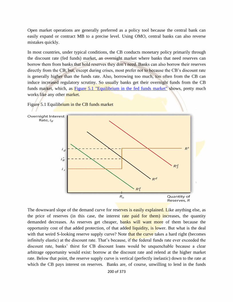
200 of 373

Open market operations are generally preferred as a policy tool because the central bank can

easily expand or contract MB to a precise level. Using OMO, central banks can also reverse

mistakes quickly.

In most countries, under typical conditions, the CB conducts monetary policy primarily through

the discount rate (fed funds) market, an overnight market where banks that need reserves can

borrow them from banks that hold reserves they don’t need. Banks can also borrow their reserves

directly from the CB, but, except during crises, most prefer not to because the CB’s discount rate

is generally higher than the funds rate. Also, borrowing too much, too often from the CB can

induce increased regulatory scrutiny. So usually banks get their overnight funds from the CB

funds market, which, as Figure 5.1 "Equilibrium in the fed funds market" shows, pretty much

works like any other market.

Figure 5.1 Equilibrium in the CB funds market

The downward slope of the demand curve for reserves is easily explained. Like anything else, as

the price of reserves (in this case, the interest rate paid for them) increases, the quantity

demanded decreases. As reserves get cheaper, banks will want more of them because the

opportunity cost of that added protection, of that added liquidity, is lower. But what is the deal

with that weird S-looking reserve supply curve? Note that the curve takes a hard right (becomes

infinitely elastic) at the discount rate. That’s because, if the federal funds rate ever exceeded the

discount rate, banks’ thirst for CB discount loans would be unquenchable because a clear

arbitrage opportunity would exist: borrow at the discount rate and relend at the higher market

rate. Below that point, the reserve supply curve is vertical (perfectly inelastic) down to the rate at

which the CB pays interest on reserves. Banks are, of course, unwilling to lend in the funds

201 of 373

market at a rate below what the CB will pay it, so the curve again becomes flat (infinitely

elastic).

The intersection of the supply and demand curves is the equilibrium or market rate, the actual

funds rate, ff*. When the CB makes open market purchases, the supply of reserves shifts right,

lowering ff* (ceteris paribus). When it sells, it moves the reserve supply curve left, increasing

ff*, all else constant. In most circumstances, the discount and reserve rates effectively channel

the market federal funds rate into a range.

Theoretically, the CB could also directly affect the demand for reserves by changing the reserve

requirement. If it increased (decreased) rr, demand for reserves would shift up (down), increasing

(decreasing) ff*. As noted above, however, banks these days can so easily sidestep required

reserves that the CB’s ability to influence the demand for reserves is extremely limited. Demand

for reserves (excess reserves that is) can also shift right or left due to bank liquidity management

activities, increasing (decreasing) as expectations of net deposit outflows increase (decrease).

Cbs try to anticipate such shifts and generally have done a good job of counteracting changes in

excess reserves through OMO. Going into holidays, for example, banks often hold a little extra

vault cash (a form of reserves). Knowing this, the CB counteracts the rightward shift in demand

(which would increase ff*) by shifting the reserve supply curve to the right by buying bonds

(thereby decreasing ff* by an offsetting amount).

Interrelations Among Goals, Targets and Instruments of Monetary Policy

In this subsection, I shall provide further information on the goals and instruments of monetary

Policy based on Handa (2009).

Besides the concepts of goals and instruments, other concepts relevant to monetary policy are

those of targets, operating targets and guides. We can broadly define a target variable as one

whose value the policy maker wants to change. An operating target variable is one on which the

central bank can directly or almost directly operate through the instruments at its disposal. A

guide is a variable that provides information on the current and future state of the economy.

Between the goals and instruments of monetary policy lie layers of intervening variables. For

example, suppose the central bank wants to reduce the inflation rate. To do so, it needs to reduce

aggregate demand in the economy. The reduction in aggregate demand usually requires a

reduction in investment and/or consumption, which requires an increase in market interest rates.

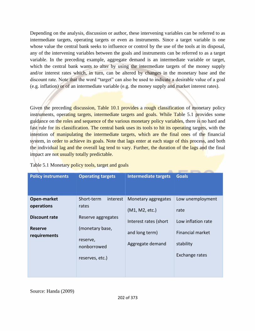
202 of 373

Depending on the analysis, discussion or author, these intervening variables can be referred to as

intermediate targets, operating targets or even as instruments. Since a target variable is one

whose value the central bank seeks to influence or control by the use of the tools at its disposal,

any of the intervening variables between the goals and instruments can be referred to as a target

variable. In the preceding example, aggregate demand is an intermediate variable or target,

which the central bank wants to alter by using the intermediate targets of the money supply

and/or interest rates which, in turn, can be altered by changes in the monetary base and the

discount rate. Note that the word “target” can also be used to indicate a desirable value of a goal

(e.g. inflation) or of an intermediate variable (e.g. the money supply and market interest rates).

Given the preceding discussion, Table 10.1 provides a rough classification of monetary policy

instruments, operating targets, intermediate targets and goals. While Table 5.1 provides some

guidance on the roles and sequence of the various monetary policy variables, there is no hard and

fast rule for its classification. The central bank uses its tools to hit its operating targets, with the

intention of manipulating the intermediate targets, which are the final ones of the financial

system, in order to achieve its goals. Note that lags enter at each stage of this process, and both

the individual lag and the overall lag tend to vary. Further, the duration of the lags and the final

impact are not usually totally predictable.

Table 5.1 Monetary policy tools, target and goals

Policy instruments

Operating targets Intermediate targets Goals

Open-market

operations

Discount rate

Reserve

requirements

Short-term interest

rates

Reserve aggregates

(monetary base,

reserve,

nonborrowed

reserves, etc.)

Monetary aggregates

(M1, M2, etc.)

Interest rates (short

and long term)

Aggregate demand

Low unemployment

rate

Low inflation rate

Financial market

stability

Exchange rates

Source: Handa (2009)

203 of 373

Relationship between goals, targets and instruments, and difficulties in the pursuit of monetary

policy

Several issues arise in the selection and use of goals, intermediate variables and operating targets

or instruments by the monetary authorities. Among these are:

Are the relationships between the ultimate goal variables, intermediate variables and operating

targets stable and predictable?

Can the central bank achieve the desired levels of the operating targets through the instruments at

its disposal?

What are the lags in these relationships, and, if they are long, can the future course of the

economy be reasonably well predicted?

To illustrate these points, let the relevant relationships be:

y = f (x;Ψ) (1)

x = g(z; θ) (2)

where:

y = (ultimate) goal variable

x = intermediate target

z = policy instrument or operating target

Ψ,θ = sets of exogenous variables

The above equations imply that:

y = h(z;Ψ,θ) (3)

204 of 373

so that z can be used to achieve a desired value of y. However, this can be done reliably only if

the functional forms f and g are known and these are stable univalued functions. In practice,

given the complex structure of the real-world economies, as well as the existence of uncertainty

and lags in the actual relationships, the precise forms of f, g and h are often only imperfectly

known at the time the decisions are made. Further, the coefficients in these relationships may be

subject to stochastic changes. In addition, given the lags in the economy, the policy maker also

needs to predict the future values of the coefficients and the exogenous

variables – again, usually an imprecise art.

Hence, the precision and clarity implied by (3) for the formulation of monetary policy and its

effects is misleading. In many, if not most instances, the impact of a change in most of the

potential operating variables on the ultimate goals is likely to be imprecise, difficult to predict

and/or unstable. This makes the formulation of monetary policy an art rather than a science and

cautions against attempts to use monetary policy as a precise control mechanism for “fine-

tuning” the goals of such policy.

Another common problem with most target variables is that they are endogenous and their values

depend on both demand and supply factors, so that the exogenous shocks to them could come

from either demand or supply shifts. The policy maker may want to offset the effect of changes

in some of these factors but not in all cases, so that it needs to know the source of such changes

before formulating its policy.

Targets of Monetary Policy

The two main operating targets usually suggested for monetary policy are:

monetary aggregates;

interest rates.

205 of 373

The two main targets of monetary policy highlighted in the recent literature are:

inflation rate (or the price level),4 or its deviation from a desired value;

output, or its deviation from the full-employment level.

There are also other variables that are sometimes used or proposed as the intermediate targets of

monetary policy. Among these is aggregate demand (or nominal national income) and, in the

case of relatively open economies, the exchange rate or the balance of payments.

Following Handa (2009), this section discusses only the relative merits and demerits of monetary

aggregates and the interest rate as the chief operating target or instruments. It also presents some

discussion of the price level and the inflation rate, and the output gap, as the targets of monetary

policy.

Monetary Aggregates versus Interest Rates as Operating Targets

This section relies upon students’ prior knowledge of the IS–LM macroeconomic model, to

distinguish between the relative merits of using the money supply versus interest rates as the

operating target of monetary policy. The choice between monetary aggregates and the interest

rate depends critically upon the policy objective of the central bank and the structure of the

economy. The following analysis, adapted from that in Poole (1970), takes this objective to be

control of aggregate demand, since the central bank can only influence output and inflation,

which are its final goal variables, through manipulation of aggregate demand. It further assumes

that the structure of the economy can be represented by the IS–LM analysis and diagram. This

diagram has aggregate real demand y on its horizontal axis and the real interest rate r on its

vertical axis. The commodity market equilibrium is shown by the IS curve and the money market

equilibrium is shown by the LM curve. Their intersection determines real aggregate demand at

the existing price level.

Therefore, the choice between the monetary instrument hinges on the question: which instrument

provides better control over aggregate demand in the IS–LM framework? Our analysis implicitly

206 of 373

assumes the Fisher equation for perfect capital markets and an expected inflation rate of zero, so

that the nominal interest rate R is identical with the real interest rate r.

This section presents first the diagrammatic analyses of monetary versus interest rate targeting

and then followed by its mathematical version.

Diagrammatic analysis of the choice of the operating target of monetary policy

Shocks arising from the commodity market

The IS equation and curve encompass the various components of expenditures, such as

consumption, investment, exports, fiscal deficits, etc., in the economy. Several of these are

volatile, with investment often being the most volatile component of expenditures. Shifts in any

of these components shift the IS curve in the IS–LM diagram.

Our analysis starts with the initial equilibrium shown by point a, with coordinates (r0, y0), in

Figure 5.1a. Assume that the central bank targets the money supply and holds it constant through

open market operations or by the use of some other instruments. Shocks to the IS curve would

then change both r and y. To illustrate, if a positive shock shifts the IS curve from IS0 to IS1,

aggregate demand will increase from y0 to y1 and the interest rate rise from r0 to r1. Similarly, a

negative shock, occurring, say, in the following period, which shifts the IS curve to IS2, will

lower aggregate demand to y2 and the interest rate to r2.

Compare this result with the impact of the same shock if the interest rate had been targeted. This

is shown in Figure 5.3, where the interest rate is assumed to be held fixed by the authorities at

the target rate r0, where the underline indicates that it is exogenously set by the central bank. The

shifts in the IS curve, first to IS1 and then to IS2, will produce movements in aggregate demand,

first to y1 and then to y2. This fluctuation between y1 and y2 is clearly greater than between y1

and y2 in Figure 5.4, so that targeting the interest rate produces greater fluctuations in aggregate

demand than money supply targeting if the exogenous shocks emanate from the commodity

market.

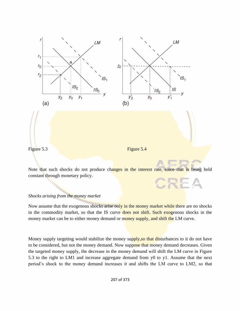
207 of 373

Figure 5.3 Figure 5.4

Note that such shocks do not produce changes in the interest rate, since that is being held

constant through monetary policy.

Shocks arising from the money market

Now assume that the exogenous shocks arise only in the money market while there are no shocks

in the commodity market, so that the IS curve does not shift. Such exogenous shocks in the

money market can be to either money demand or money supply, and shift the LM curve.

Money supply targeting would stabilize the money supply,so that disturbances to it do not have

to be considered, but not the money demand. Now suppose that money demand decreases. Given

the targeted money supply, the decrease in the money demand will shift the LM curve in Figure

5.3 to the right to LM1 and increase aggregate demand from y0 to y1. Assume that the next

period’s shock to the money demand increases it and shifts the LM curve to LM2, so that

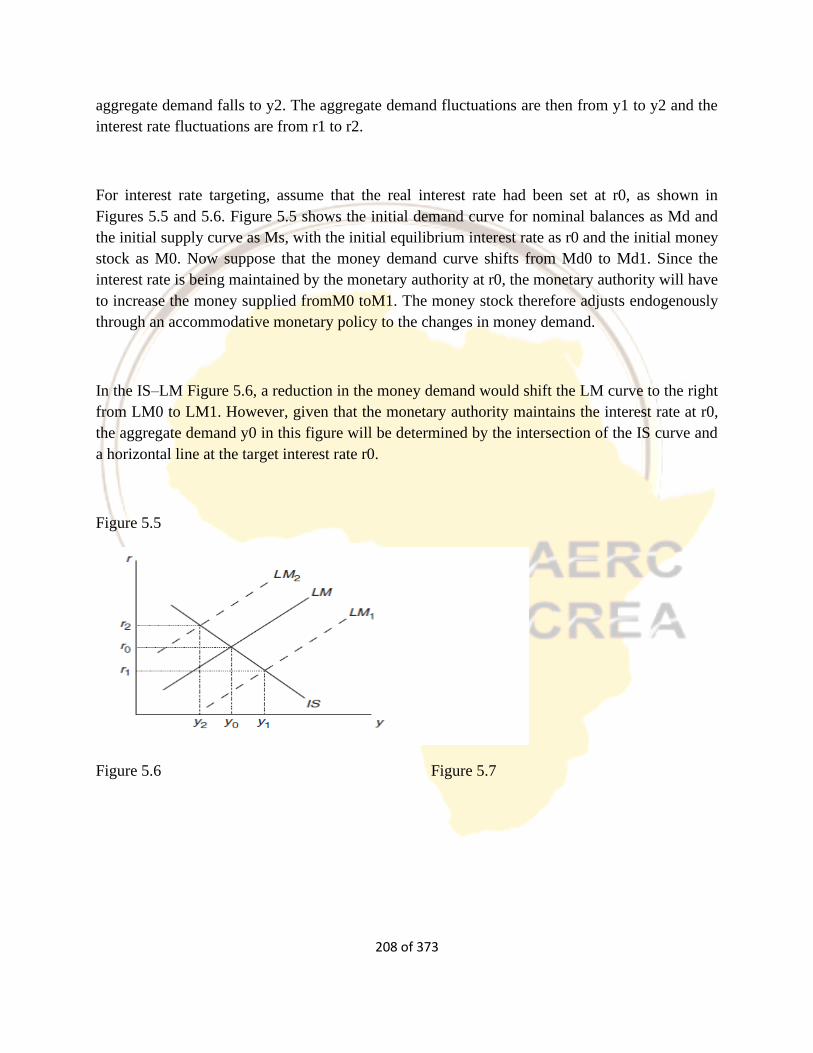
208 of 373

aggregate demand falls to y2. The aggregate demand fluctuations are then from y1 to y2 and the

interest rate fluctuations are from r1 to r2.

For interest rate targeting, assume that the real interest rate had been set at r0, as shown in

Figures 5.5 and 5.6. Figure 5.5 shows the initial demand curve for nominal balances as Md and

the initial supply curve as Ms, with the initial equilibrium interest rate as r0 and the initial money

stock as M0. Now suppose that the money demand curve shifts from Md0 to Md1. Since the

interest rate is being maintained by the monetary authority at r0, the monetary authority will have

to increase the money supplied fromM0 toM1. The money stock therefore adjusts endogenously

through an accommodative monetary policy to the changes in money demand.

In the IS–LM Figure 5.6, a reduction in the money demand would shift the LM curve to the right

from LM0 to LM1. However, given that the monetary authority maintains the interest rate at r0,

the aggregate demand y0 in this figure will be determined by the intersection of the IS curve and

a horizontal line at the target interest rate r0.

Figure 5.5

Figure 5.6 Figure 5.7

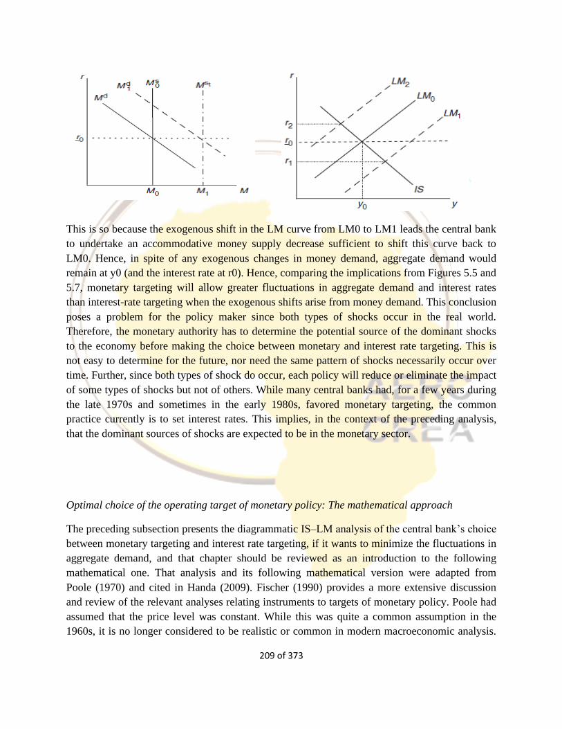
209 of 373

This is so because the exogenous shift in the LM curve from LM0 to LM1 leads the central bank

to undertake an accommodative money supply decrease sufficient to shift this curve back to

LM0. Hence, in spite of any exogenous changes in money demand, aggregate demand would

remain at y0 (and the interest rate at r0). Hence, comparing the implications from Figures 5.5 and

5.7, monetary targeting will allow greater fluctuations in aggregate demand and interest rates

than interest-rate targeting when the exogenous shifts arise from money demand. This conclusion

poses a problem for the policy maker since both types of shocks occur in the real world.

Therefore, the monetary authority has to determine the potential source of the dominant shocks

to the economy before making the choice between monetary and interest rate targeting. This is

not easy to determine for the future, nor need the same pattern of shocks necessarily occur over

time. Further, since both types of shock do occur, each policy will reduce or eliminate the impact

of some types of shocks but not of others. While many central banks had, for a few years during

the late 1970s and sometimes in the early 1980s, favored monetary targeting, the common

practice currently is to set interest rates. This implies, in the context of the preceding analysis,

that the dominant sources of shocks are expected to be in the monetary sector.

Optimal choice of the operating target of monetary policy: The mathematical approach

The preceding subsection presents the diagrammatic IS–LM analysis of the central bank’s choice

between monetary targeting and interest rate targeting, if it wants to minimize the fluctuations in

aggregate demand, and that chapter should be reviewed as an introduction to the following

mathematical one. That analysis and its following mathematical version were adapted from

Poole (1970) and cited in Handa (2009). Fischer (1990) provides a more extensive discussion

and review of the relevant analyses relating instruments to targets of monetary policy. Poole had

assumed that the price level was constant. While this was quite a common assumption in the

1960s, it is no longer considered to be realistic or common in modern macroeconomic analysis.

210 of 373

Further, taking the price level as constant, Poole assumed that the central bank’s objective was to

minimize the variance of real output. Since the following analysis does not assume a constant

price level and the central bank can only affect output through aggregate demand and

expenditures, it makes the assumption that the central bank wants to minimize the variance of

aggregate demand.

Assume that the IS and LM equations each have a disturbance term. Further, assume that the

central bank can control the economy’s interest rate r and money supply Ms except for

uncontrollable disturbance terms and ηt , so that:

IS: 𝑦𝑡𝑑 = −∝𝑟 𝑟𝑡 − 𝜇𝑡

LM: (MP⁄ )t = −m1Rr + m2yt

d + ηt

where:

the demand for real balances md is a function of real income y and the nominal interest rate r snd

assuming a linear relationship for simplification for the demand for real balances, specified by:

md = md (y, R, FW0) = myy+(FW0 −mRR)

and

m = real money balances

myy = real transactions balances

(FW0 −mRR) = speculative/portfolio demand for real balances

mRR = portfolio demand for bonds

R = nominal interest rate

FW0 = real financial wealth

This IS–LM model needs to be supplemented by a relationship between rt and Rt . This is

provided, for an economy with perfect capital markets, by the Fisher equation:

211 of 373

𝑅𝑡 = 𝑟𝑡 + 𝜋𝑡𝑒

where 𝜋𝑡𝑒 is the expected inflation rate for period t. Holding these expectations constant as a

simplifying analytical assumption, Rt and rt can be treated as identical in the IS–LM model.

Hence, replacing Rt by rt in the LM equation, the model becomes:

𝐼𝑆: 𝑦𝑡𝑑 = −𝛼𝑟 + 𝜇𝑡 ……………………………………………………..(1

𝐿𝑀: (𝑀𝑃⁄ )𝑡 = −𝑚1𝑟𝑟 + 𝑚2𝑦𝑡

𝑑 + 𝜂𝑡 …………………………………….(2

The central bank observes the values of all terms, except those of the shocks, prior to setting its

policy instrument, which is either Mt or rt . Its objective function is to minimize the expected

variance of aggregate demand around its trend value, i.e.

minimize E(𝑦𝑡𝑑)2

Since y has been defined in terms of deviations from its trend, note that the equilibrium value

of 𝑦𝑡𝑑 in the absence of shocks (μ = η = 0) would be zero, so that its variance arises only by

virtue of μ and η being different from zero.

When the money stock is the policy instrument, we need to solve (1) and (2) to derive 𝑦𝑡𝑑

which is given by:

𝐼𝑆 − 𝐿𝑀: 𝑦𝑡𝑑 =

(𝛼𝑟𝑀

𝑃⁄ )+𝑚1𝜇𝑡 −𝛼𝑟𝜂𝑡

𝛼𝑟𝑚2+𝑚1……………………………(3)

Since Eμ = Eη = 0, E(yd) = (𝛼𝑟

𝑀𝑃⁄ )

𝛼𝑟𝑚2+𝑚1 . Hence, noting that the variables in the current

model are being defined in terms of deviations from their trend values, targeting M such that

E(𝑦𝑡𝑑 ) = 0 requires M/P = 0, which yields:

𝑦𝑡𝑑 =

𝑚1𝜇𝑡 −𝛼𝑟𝜂𝑡

𝛼𝑟𝑚2+𝑚1 ……………………………………………………………..(4)

Therefore, under the assumption that μ and η are uncorrelated and the variance of αP is zero, the

variance of aggregate demand under the money supply instrument is

given by,

𝐸𝑑(𝑦𝑑)2 =𝑚1

2𝜎𝜇2+𝛼𝑟

2𝜎𝜂2

(𝛼𝑟𝑚2+𝑚1)2…………………………….(5)

212 of 373

where the superscript m on E indicates monetary targeting. When the real interest rate is the

monetary policy instrument, the IS equation (1) alone needs to be solved for 𝑦𝑡𝑑. Under interest

rate targeting, setting r such that E(𝑦𝑡𝑑) = 0, its variance becomes:

𝐸𝑟(𝑦𝑑)2 = 𝜎𝜇2 ……………………………………..(6)

where the superscript r on E indicates interest rate targeting. Monetary targeting is preferable

to interest rate targeting if (5) is less than (6), and vice versa. The former requires:

𝑚12𝜎𝜇

2+𝛼𝑟2𝜎𝜂

2

(𝛼𝑟𝑚2+𝑚1)2 < 𝜎𝜇2 (7)

Which simplifies to:

𝜎𝜂2 < 𝜎𝜇

2(𝑚22 +

2𝑚2𝑚1

𝛼𝑟 (8)

Hence, if there are only money market shocks but no commodity market shocks (i.e.σμ = 0), then

interest rate targeting is preferable since doing so perfectly stabilizes aggregate demand; the LM

equation and its disturbance term become irrelevant to the determination of aggregate demand.

But if there are only commodity market shocks but no money market shocks (i.e. ση = 0), then

monetary targeting is preferable since doing so reduces fluctuations in aggregate demand. In this

case, with a given money supply, a positive commodity market shock raises the interest rate,

which reduces interest-sensitive expenditures, thereby reducing commodity demand, so that the

original shock to demand is partially offset.

In the general case, the choice of the policy instrument will depend on the relative magnitudes of

the shocks and the slope of the IS curve (whose slope is −1/αr) relative to that of the LM curve

(whose slope is 1/mr ). If, for simplification, the term in parentheses on the right-hand side of

(8) were ignored, monetary targeting would be preferable to interest rate targeting if the

stochastic disturbance in the money market were smaller than in the commodity market. For the

money market, assuming that the central bank can precisely control the money supply but does

not know the money demand because of the instability of this demand, ση occurs because of the

volatility of money demand.

For the commodity market, if we were to assume that the instability of commodity demand arises

only because of the instability of investment (though consumption and net exports can also be

volatile), σμ occurs because of the volatility of investment demand. These assumptions provide

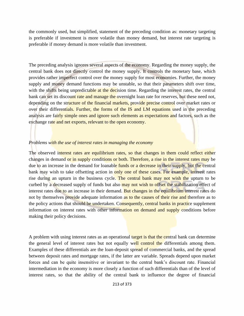
213 of 373

the commonly used, but simplified, statement of the preceding condition as: monetary targeting

is preferable if investment is more volatile than money demand, but interest rate targeting is

preferable if money demand is more volatile than investment.

The preceding analysis ignores several aspects of the economy. Regarding the money supply, the

central bank does not directly control the money supply. It controls the monetary base, which

provides rather imperfect control over the money supply for most economies. Further, the money

supply and money demand functions may be unstable, so that their parameters shift over time,

with the shifts being unpredictable at the decision time. Regarding the interest rates, the central

bank can set its discount rate and manage the overnight loan rate for reserves, but these need not,

depending on the structure of the financial markets, provide precise control over market rates or

over their differentials. Further, the forms of the IS and LM equations used in the preceding

analysis are fairly simple ones and ignore such elements as expectations and factors, such as the

exchange rate and net exports, relevant to the open economy.

Problems with the use of interest rates in managing the economy

The observed interest rates are equilibrium rates, so that changes in them could reflect either

changes in demand or in supply conditions or both. Therefore, a rise in the interest rates may be

due to an increase in the demand for loanable funds or a decrease in their supply, but the central

bank may wish to take offsetting action in only one of these cases. For example, interest rates

rise during an upturn in the business cycle. The central bank may not wish the upturn to be

curbed by a decreased supply of funds but also may not wish to offset the stabilization effect of

interest rates due to an increase in their demand. But changes in the equilibrium interest rates do

not by themselves provide adequate information as to the causes of their rise and therefore as to

the policy actions that should be undertaken. Consequently, central banks in practice supplement

information on interest rates with other information on demand and supply conditions before

making their policy decisions.

A problem with using interest rates as an operational target is that the central bank can determine

the general level of interest rates but not equally well control the differentials among them.

Examples of these differentials are the loan-deposit spread of commercial banks, and the spread

between deposit rates and mortgage rates, if the latter are variable. Spreads depend upon market

forces and can be quite insensitive or invariant to the central bank’s discount rate. Financial

intermediation in the economy is more closely a function of such differentials than of the level of

interest rates, so that the ability of the central bank to influence the degree of financial

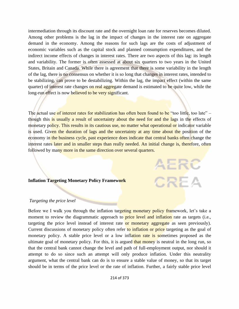
214 of 373

intermediation through its discount rate and the overnight loan rate for reserves becomes diluted.

Among other problems is the lag in the impact of changes in the interest rate on aggregate

demand in the economy. Among the reasons for such lags are the costs of adjustment of

economic variables such as the capital stock and planned consumption expenditures, and the

indirect income effects of changes in interest rates. There are two aspects of this lag: its length

and variability. The former is often assessed at about six quarters to two years in the United

States, Britain and Canada. While there is agreement that there is some variability in the length

of the lag, there is no consensus on whether it is so long that changes in interest rates, intended to

be stabilizing, can prove to be destabilizing. Within the lag, the impact effect (within the same

quarter) of interest rate changes on real aggregate demand is estimated to be quite low, while the

long-run effect is now believed to be very significant.

The actual use of interest rates for stabilization has often been found to be “too little, too late” –

though this is usually a result of uncertainty about the need for and the lags in the effects of

monetary policy. This results in its cautious use, no matter what operational or indicator variable

is used. Given the duration of lags and the uncertainty at any time about the position of the

economy in the business cycle, past experience does indicate that central banks often change the

interest rates later and in smaller steps than really needed. An initial change is, therefore, often

followed by many more in the same direction over several quarters.

Inflation Targeting Monetary Policy Framework

Targeting the price level

Before we I walk you through the inflation targeting monetary policy framework, let’s take a

moment to review the diagrammatic approach to price level and inflation rate as targets (i.e.,

targeting the price level instead of interest rate or monetary aggregate as seen previously).

Current discussions of monetary policy often refer to inflation or price targeting as the goal of

monetary policy. A stable price level or a low inflation rate is sometimes proposed as the

ultimate goal of monetary policy. For this, it is argued that money is neutral in the long run, so

that the central bank cannot change the level and path of full-employment output, nor should it

attempt to do so since such an attempt will only produce inflation. Under this neutrality

argument, what the central bank can do is to ensure a stable value of money, so that its target

should be in terms of the price level or the rate of inflation. Further, a fairly stable price level

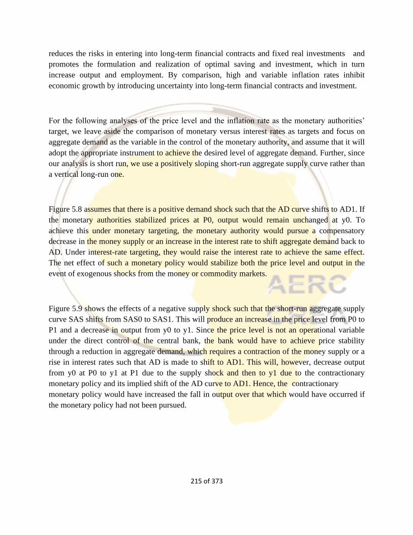
215 of 373

reduces the risks in entering into long-term financial contracts and fixed real investments and

promotes the formulation and realization of optimal saving and investment, which in turn

increase output and employment. By comparison, high and variable inflation rates inhibit

economic growth by introducing uncertainty into long-term financial contracts and investment.

For the following analyses of the price level and the inflation rate as the monetary authorities’

target, we leave aside the comparison of monetary versus interest rates as targets and focus on

aggregate demand as the variable in the control of the monetary authority, and assume that it will

adopt the appropriate instrument to achieve the desired level of aggregate demand. Further, since

our analysis is short run, we use a positively sloping short-run aggregate supply curve rather than

a vertical long-run one.

Figure 5.8 assumes that there is a positive demand shock such that the AD curve shifts to AD1. If

the monetary authorities stabilized prices at P0, output would remain unchanged at y0. To

achieve this under monetary targeting, the monetary authority would pursue a compensatory

decrease in the money supply or an increase in the interest rate to shift aggregate demand back to

AD. Under interest-rate targeting, they would raise the interest rate to achieve the same effect.

The net effect of such a monetary policy would stabilize both the price level and output in the

event of exogenous shocks from the money or commodity markets.

Figure 5.9 shows the effects of a negative supply shock such that the short-run aggregate supply

curve SAS shifts from SAS0 to SAS1. This will produce an increase in the price level from P0 to

P1 and a decrease in output from y0 to y1. Since the price level is not an operational variable

under the direct control of the central bank, the bank would have to achieve price stability

through a reduction in aggregate demand, which requires a contraction of the money supply or a

rise in interest rates such that AD is made to shift to AD1. This will, however, decrease output

from y0 at P0 to y1 at P1 due to the supply shock and then to y1 due to the contractionary

monetary policy and its implied shift of the AD curve to AD1. Hence, the contractionary

monetary policy would have increased the fall in output over that which would have occurred if

the monetary policy had not been pursued.

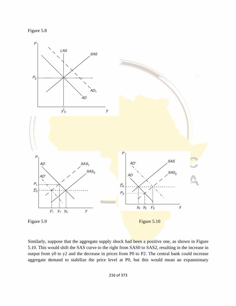
216 of 373

Figure 5.8

Figure 5.9 Figure 5.10

Similarly, suppose that the aggregate supply shock had been a positive one, as shown in Figure

5.10. This would shift the SAS curve to the right from SAS0 to SAS2, resulting in the increase in

output from y0 to y2 and the decrease in prices from P0 to P2. The central bank could increase

aggregate demand to stabilize the price level at P0, but this would mean an expansionary

217 of 373

monetary policy which shifts the AD curve to AD1 and further increases output to y2. Price

stabilization has, therefore, again increased the fluctuation in output.

Therefore, given the aggregate supply curve as being positively sloped and short run, the pursuit

of price stability in the face of supply-side fluctuations has the cost of. I shall leave it to you to

adapt the analysis to the case of a vertical long-run supply curve.

Inflation Targeting Policy Framework

Inflation targeting, which simply involves a central bank raising or lowering interest rates to

anchor inflation expectations in order to achieve a given inflation target, has been recognized

mostly in developed world as a more effective way of maintaining low and stable inflation. The

conventional wisdom is that raising interest rates usually cools the economy to rein in inflation.

The issue is that there is no long-term trade-off between inflation and output and that price

stability stimulates growth.

The recognition that price stability should be the primary long-run goal of monetary policy and

that a nominal anchor is a valuable tool in helping to achieve this goal has led to a monetary

policy strategy known as inflation targeting (Mishkin 2014). Inflation targeting involves several

elements:

public announcement of medium-term numerical objectives (targets) for inflation;

an institutional commitment to price stability as the primary, long-run goal of monetary policy

and a commitment to achieving the inflation goal;

an information-inclusive approach in which many variables (not just monetary aggregates) are

used in making decisions about monetary policy;

increased transparency of the monetary policy strategy through communication with the public

and the markets about the plans and objectives of monetary policymakers; and

increased accountability of the central bank for attaining its inflation objectives.

New Zealand was the first country to formally adopt inflation targeting in 1990, followed by

Canada in 1991, the United Kingdom in 1992, Sweden and Finland in 1993, and Australia and

Spain in 1994. Israel, Chile, and Brazil, among other countries, have also adopted a form of

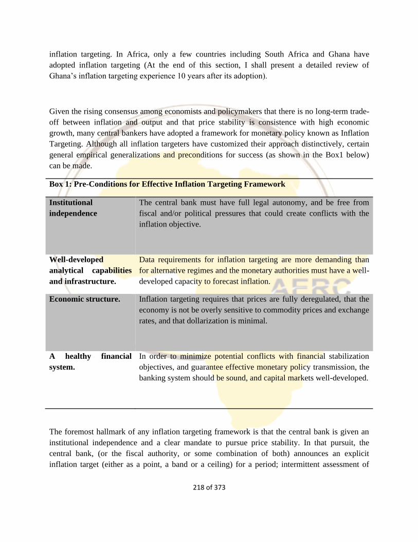
218 of 373

inflation targeting. In Africa, only a few countries including South Africa and Ghana have

adopted inflation targeting (At the end of this section, I shall present a detailed review of

Ghana’s inflation targeting experience 10 years after its adoption).

Given the rising consensus among economists and policymakers that there is no long-term trade-

off between inflation and output and that price stability is consistence with high economic

growth, many central bankers have adopted a framework for monetary policy known as Inflation

Targeting. Although all inflation targeters have customized their approach distinctively, certain

general empirical generalizations and preconditions for success (as shown in the Box1 below)

can be made.

Box 1: Pre-Conditions for Effective Inflation Targeting Framework

Institutional

independence

The central bank must have full legal autonomy, and be free from

fiscal and/or political pressures that could create conflicts with the

inflation objective.

Well-developed

analytical capabilities

and infrastructure.

Data requirements for inflation targeting are more demanding than

for alternative regimes and the monetary authorities must have a well-

developed capacity to forecast inflation.

Economic structure. Inflation targeting requires that prices are fully deregulated, that the

economy is not be overly sensitive to commodity prices and exchange

rates, and that dollarization is minimal.

A healthy financial

system.

In order to minimize potential conflicts with financial stabilization

objectives, and guarantee effective monetary policy transmission, the

banking system should be sound, and capital markets well-developed.

The foremost hallmark of any inflation targeting framework is that the central bank is given an

institutional independence and a clear mandate to pursue price stability. In that pursuit, the

central bank, (or the fiscal authority, or some combination of both) announces an explicit

inflation target (either as a point, a band or a ceiling) for a period; intermittent assessment of

219 of 373

inflationary pressures over the relevant time horizon; and systematic adjustments in the monetary

policy tool based on pressure within the operating environment.

As inflation targeting is forward-looking, a prerequisite that underpins its success, is a well-

functioning inflation forecasting framework and an efficient financial market that is responsive.

As established in practice thus far, inflation targeting central banks maintain significant scope for

applying discretion in the conduct of monetary policy. Thus, a good judgment on their part is a

critical element for successful inflation targeting.

Achieving the target was crucial to realizing policy credibility and anchoring expectations of

economic agents about monetary policy. Truly, having an autonomous central bank with an overt

mandate and quantifiable inflation target is desirous, but it has else diminished the crux of using

monetary policy to achieve other essential economic goal. The centrality of the central bank on

aggressive inflation targeting is counterproductive in a country characterized with weak fiscal

and productive fundamentals6.

Several empirical studies into the effectiveness of IT in reducing inflation have been undertaken.

Two main contrasting conclusion are drawn from available empirical literature: while some

economists agree inflation targeting effects no statistical difference on inflation (Huh, 1996;

Bernanke and Mihov, 1998; Lane and van den Heuvel, 1998; Bernankeet al., 1999; Honda, 2000;

da Silva and Portugal, 2000; Ball and Sherridan, 2003) others provide evidence that the

framework does cause structural break in the inflation rate trend (Almeida and Goodhart, 1996;

Batini and Laxton, 1994; Fillion and Le´onard, 1997; Choiet al., 2003; Pe´tursson, 2004;

Mishkin, 2007). Mishkin (2007, p. 406) asserted that IT has firmly anchored inflation

expectations and inflation beyond the counterfactual (what would be the case under no IT). His

assertion supported that of Condon (2006) in the case of Korea.

Bernanke et al., (1999) while favoring inflation targeting, highlighted extensive evidence that the

framework’s success traded-off national output (i.e. sacrifice ratio) compared to non-targeters.

The question of whether IT will succeed in developing nations was addressed by Mishkin and

Savastano (2002) who reported that IT will only be successful (and not sacrifice economic

growth) if and only if standard initial conditions of central bank operational independence,

absence of fiscal and financial dominance, and moderately low inflation are in place. This

position was further reinforced by Stiglitz (2008). Stiglitz debased inflation targeting as a crude

recipe for developing nations as long as they do not integrate themselves of the international

shocks by restructuring their economic fundamentals.

6 See Bernanke, et. al, 1999 and Epstein, 2000, for detailed surveys of the literature

220 of 373

According to Mishkin (2010), an important criticism of inflation targeting is that a sole focus on

inflation may lead to monetary policy that is too tight when inflation is above target and thus

may lead to output fluctuations, lower economic growth and high unemployment.

Advantages of Inflation Targeting

There are a number of benefits associated with inflation targeting: reduction of the time

inconsistency problem, increased transparency, increased accountability, consistency with

democratic principles, and improved performance.

Reduction of the Time-Inconsistency Problem Because an explicit numerical inflation target

increases the accountability of the central bank, inflation targeting can reduce the likelihood that

the central bank will fall into the time-inconsistency trap of trying to expand output and

employment in the short run by pursuing overly expansionary monetary policy. A key advantage

of inflation targeting is that it can help focus the political debate on what a central bank can do in

the long run—that is, control inflation—rather than what it cannot do, that is, permanently

increase economic growth and the number of jobs through expansionary monetary policy. Thus

inflation targeting can reduce political pressures on the central bank to pursue inflationary

monetary policy and thereby reduce the likelihood of the time-inconsistency problem.

Increased Transparency: Inflation targeting has the advantage that it is readily understood by the

public and is thus highly transparent. Indeed, inflation-targeting regimes place great importance

on transparency in policymaking and on regular communication with the public. Inflation-

targeting central banks have frequent communications with the government, some mandated by

law and some in response to informal inquiries, and their officials take every opportunity to

make public speeches on their monetary policy strategy. Although these techniques are also

commonly used in countries that have not adopted inflation targeting, inflation-targeting central

banks have taken public outreach a step further: Not only do they engage in extended public

information campaigns, including the distribution of glossy brochures, but they also publish

documents like the Bank of England’s Inflation Report. These documents are particularly

noteworthy because, unlike the usual dull-looking, formal reports of central banks, they make

use of fancy graphics, boxes, and other eye-catching design elements to engage the public’s

interest.

The channels of communication just discussed are used by central banks in inflation-targeting

countries to explain the following concepts to the general public, financial market participants,

221 of 373

and politicians: (1) the goals and limitations of monetary policy, including the rationale for

inflation targets; (2) the numerical values of the inflation targets and how they were determined;

(3) how the inflation targets are to be achieved, given current economic conditions; and (4)

reasons for any deviations from the targets. These communications have improved private sector

planning by reducing uncertainty about monetary policy, interest rates, and inflation; they have

promoted public debate of monetary policy, in part by educating the public about what a central

bank can and cannot achieve; and they have helped clarify the responsibilities of the central bank

and of politicians in the conduct of monetary policy.

Increased Accountability: Another key feature of inflation-targeting regimes is the tendency

toward increased accountability of the central bank. Indeed, transparency and communication go

hand in hand with increased accountability. The strongest case of accountability of a central bank

in an inflation-targeting regime is in New Zealand, where the government has the right to dismiss

the Reserve Bank’s governor if the inflation targets are breached, even for one quarter. In other

inflation-targeting countries, the central bank’s accountability is less formalized. Nevertheless,

the transparency of policy associated with inflation targeting has tended to make the central bank

highly accountable to the public and the government. Sustained success in the conduct of

monetary policy as measured against a preannounced and well-defined inflation target can be

instrumental in building public support for a central bank’s independence and for its policies.

This building of public support and accountability occurs even in the absence of a rigidly defined

and legalistic standard of performance evaluation and punishment.

Consistency with Democratic Principles: Not only is accountability valuable in its own right, but

it also makes the institutional framework for the conduct of monetary policy more consistent

with democratic principles. The inflation-targeting framework promotes the accountability of the

central bank to elected officials, who are given some responsibility for setting the goals of

monetary policy and then monitoring the economic outcomes. However, under inflation targeting

as it generally has been practiced, the central bank has complete control over operational

decisions and so can be held accountable for achieving its assigned objectives. Improved

Performance The performance of inflation-targeting regimes has been quite good. Inflation-

targeting countries seem to have significantly reduced both the rate of inflation and inflation

expectations beyond what likely would have occurred in the absence of inflation targets.

Furthermore, once lowered, inflation in these countries has stayed low; following disinflation,

the inflation rate in inflation-targeting countries has not bounced back up during subsequent

cyclical expansions of the economy.

222 of 373

Disadvantages of Inflation Targeting

Critics of inflation targeting cite four disadvantages of this monetary policy strategy: delayed

signaling, too much rigidity, the potential for increased output fluctuations, and low economic

growth. We look at each in turn and examine the validity of these criticisms. Delayed Signaling

Inflation is not easily controlled by the monetary authorities. Furthermore, because of the long

lags in the effects of monetary policy, inflation outcomes are revealed only after a substantial

lag. Thus an inflation target does not send immediate signals to the public and the markets about

the stance of monetary policy.

Too Much Rigidity Some economists criticize inflation targeting because they believe it imposes

a rigid rule on monetary policymakers and limits their ability to respond to unforeseen

circumstances. However, useful policy strategies exist that are “rule-like” in that they involve

forward-looking behavior that limits policymakers from systematically engaging in policies with

undesirable long-run consequences. Such policies avoid the time-inconsistency problem and

would be best described as “constrained discretion,” a term coined by Ben Bernanke and the

author of this book.

Indeed, inflation targeting can be described exactly in this way. Inflation targeting, as actually

practiced, is far from rigid and is better described as “flexible inflation targeting.” First, inflation

targeting does not prescribe simple and mechanical instructions on how the central bank should

conduct monetary policy. Rather, it requires the central bank to use all available information to

determine which policy actions are appropriate to achieve the inflation target. Unlike simple

policy rules, inflation targeting never requires the central bank to focus solely on one key

variable. Second, inflation targeting, as practiced, contains a substantial degree of policy

discretion.

Inflation targets have been modified depending on economic circumstances, as we have seen.

Moreover, central banks under inflation-targeting regimes have left themselves considerable

scope to respond to output growth and fluctuations through several devices.

Potential for Increased Output Fluctuations An important criticism of inflation targeting is that a

sole focus on inflation may lead to monetary policy that is too tight when inflation is above

target and thus may result in larger output fluctuations. Inflation targeting does not, however,

require a sole focus on inflation—in fact, experience has shown that inflation targeters display

223 of 373

substantial concern about output fluctuations. All the inflation targeters have set their inflation

targets above zero.3 For example, New Zealand, Canada, the United Kingdom, and Sweden

currently set the midpoints of their inflation targets at 2%, while Australia sets its midpoint at

2.5%.

Inflation targeting also does not ignore traditional stabilization goals. Central bankers in

inflation-targeting countries continue to express their concern about fluctuations in output and

employment, and the ability to accommodate short-run stabilization goals to some degree is built

into all inflation-targeting regimes. All inflation-targeting countries have been willing to

minimize output declines by gradually lowering medium-term inflation targets toward the long-

run goal.

Low Economic Growth Another common concern about inflation targeting is that it will lead to

low growth in output and employment. Although inflation reduction has been associated with

below-normal output during disinflationary phases in inflation targeting regimes, once low

inflation levels were achieved, output and employment returned to levels at least as high as they

were before. A conservative conclusion is that once low inflation is achieved, inflation targeting

is not harmful to the real economy. Given the strong economic growth after disinflation in many

countries (such as New Zealand) that have adopted inflation targets, a case can be made that

inflation targeting promotes real economic growth, in addition to controlling inflation.

Empirical Study: A case of Inflation Targeting Policy Framework in Ghana

The functional autonomy of the Bank of Ghana (BoG) in adopting inflation targeting through

the Monetary Policy Committee (MPC) to conduct monetary policy in a manner that ensures

price stability, while supporting other macroeconomic goals is guaranteed under the Bank of

Ghana Act, 2002 (Act 612) but it was not until 2007 that the Bank officially adopted an

inflation targeting framework for the conduct of monetary policy. Prior to its adoption, the

Bank of Ghana operated largely a direct controlled system of monetary framework, known as

the monetary aggregate regime with money growth as the nominal anchor in arresting

inflation.

However, a decade after the adoption of IT, Ghana’s experience under the framework has

sparked debate over its effectiveness in ensuring a low and stable price levels and in particular,

lowering interest rates as it tends to over emphasize inflation at the expense of other monetary

and macroeconomic goals, like growth and employment.

224 of 373

The large fiscal expansions coupled with unfavourable trade balances which often lead to high

inflation pressures and weakening of the domestic currency, particularly in periods

immediately after election years, had meant that the Bank of Ghana had had to adjust the

monetary policy rate (MPR) upward in many occasions in order to subdue the resultant

inflationary pressures without recourse to the negative effect on growth. This has culminated

into high interest rates, which is among the highest in Africa.

For instance, the MPR had been increased from 13.5 percent in 2010 to 26 percent by the end

of 2015 and stayed there until January 2017. Although inflation, since March 2016, had

consistently been fallen from a high of 19.2 percent to 13.3 percent in February, 2017, the

MPR remained resolute at the 26 percent until it was marginally reduced to 25.5 percent in

January and 23.5 in March this year. This situation has created a wide spread between inflation

and the MPR, as well as, between the average lending rate and inflation rate over a long period

of time. The question on the minds of many economists and civil societies is why the

monetary policy rate and lending rates have not fallen in like manner with inflation, even

though inflation is on a persistent decline.

Inflation targeting as a monetary framework combined with salient characteristics of emerging

economies especially Ghana raises important policy concerns. This is because several studies

have shown that certain characteristics of emerging markets do not support inflation targeting

framework.

Emerging market economies are often characterized by a lack of credibility and limited access

to international markets, pronounced adverse effects of exchange rate volatility on trade, fiscal

dominance, high liability dollarization, and higher pass-through from the exchange rate to

inflation. These characteristics can be a threat to inflation targeting framework for developing

economies like Ghana.

It is against this background that this paper explores the effect of inflation targeting on

inflation and interest rates in Ghana. It argues that inflation targeting in the midst of fiscal

indiscipline/persistent over expenditures and weak productive structures, as well as, low

export capacity that exposes the country to exchange rate fluctuations will not be effective and

rather results in high interest rates. It further points out that with the country characterized by

high fiscal dominance and volatile exchange rates coupled with, a very weak productive,

institutional and operational capacity, unlike most inflation targeters across the globe, inflation

targeting is perhaps not for a developing country like Ghana.

Like most performance measurement criteria, the success of any IT regime is evaluated by

comparing inflation targets with outcomes. By this, I intend to examine the magnitude of

spread between targets and recorded inflation rates compared to periods preceding inflation

targeting. In figure 1.1 below presents a time series plot of targeted inflation rates and the end

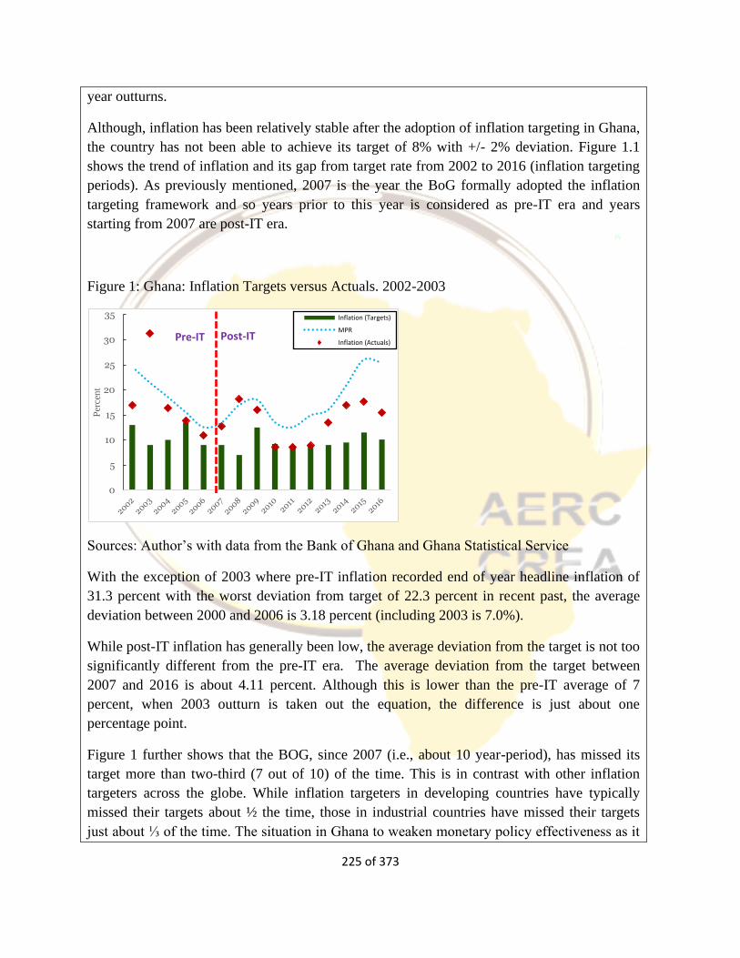
225 of 373

year outturns.

Although, inflation has been relatively stable after the adoption of inflation targeting in Ghana,

the country has not been able to achieve its target of 8% with +/- 2% deviation. Figure 1.1

shows the trend of inflation and its gap from target rate from 2002 to 2016 (inflation targeting

periods). As previously mentioned, 2007 is the year the BoG formally adopted the inflation

targeting framework and so years prior to this year is considered as pre-IT era and years

starting from 2007 are post-IT era.

Figure 1: Ghana: Inflation Targets versus Actuals. 2002-2003

Sources: Author’s with data from the Bank of Ghana and Ghana Statistical Service

With the exception of 2003 where pre-IT inflation recorded end of year headline inflation of

31.3 percent with the worst deviation from target of 22.3 percent in recent past, the average

deviation between 2000 and 2006 is 3.18 percent (including 2003 is 7.0%).

While post-IT inflation has generally been low, the average deviation from the target is not too

significantly different from the pre-IT era. The average deviation from the target between

2007 and 2016 is about 4.11 percent. Although this is lower than the pre-IT average of 7

percent, when 2003 outturn is taken out the equation, the difference is just about one

percentage point.

Figure 1 further shows that the BOG, since 2007 (i.e., about 10 year-period), has missed its

target more than two-third (7 out of 10) of the time. This is in contrast with other inflation

targeters across the globe. While inflation targeters in developing countries have typically

missed their targets about ½ the time, those in industrial countries have missed their targets

just about ⅓ of the time. The situation in Ghana to weaken monetary policy effectiveness as it

0

5

10

15

20

25

30

35

Per

cen

t

Inflation (Targets)

MPR

Inflation (Actuals)Pre-IT Post-IT

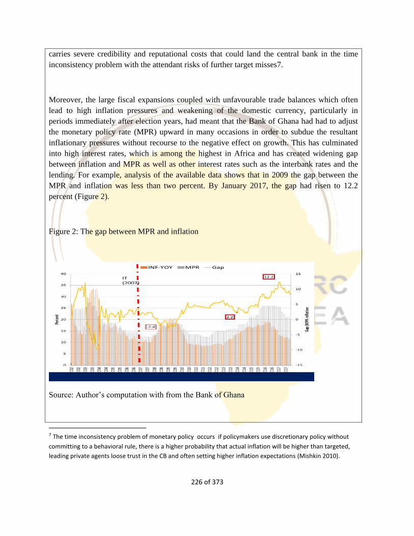
226 of 373

carries severe credibility and reputational costs that could land the central bank in the time

inconsistency problem with the attendant risks of further target misses7.

Moreover, the large fiscal expansions coupled with unfavourable trade balances which often

lead to high inflation pressures and weakening of the domestic currency, particularly in

periods immediately after election years, had meant that the Bank of Ghana had had to adjust

the monetary policy rate (MPR) upward in many occasions in order to subdue the resultant

inflationary pressures without recourse to the negative effect on growth. This has culminated

into high interest rates, which is among the highest in Africa and has created widening gap

between inflation and MPR as well as other interest rates such as the interbank rates and the

lending. For example, analysis of the available data shows that in 2009 the gap between the

MPR and inflation was less than two percent. By January 2017, the gap had risen to 12.2

percent (Figure 2).

Figure 2: The gap between MPR and inflation

Source: Author’s computation with from the Bank of Ghana

7 The time inconsistency problem of monetary policy occurs if policymakers use discretionary policy without

committing to a behavioral rule, there is a higher probability that actual inflation will be higher than targeted,

leading private agents loose trust in the CB and often setting higher inflation expectations (Mishkin 2010).

227 of 373

Concluding Remarks

Getting monetary policy right is crucial to the health of the economy and the wellbeing of its

people. As such, monetary policy should not only seek to achieve stable prices, but also seek

to affect real economic outcomes such as growth and employment in order to improve the

welfare of its citizens.

This paper has explored the effect of inflation targeting on interest rates in Ghana. It argues

that inflation targeting in the midst of fiscal indiscipline/persistent over expenditures and weak

productive structures, as well as, low export capacity that exposes the country to exchange rate

fluctuations will not be effective and rather results in high interest rates. It further points out

that with the country characterized by high fiscal dominance and volatile exchange rates

coupled with, a very weak productive, institutional and operational capacity, unlike most

inflation targeters across the globe, inflation targeting is perhaps not for a developing country

like Ghana. It observes that besides the inflation target framework resulting in high interest

rates in the country, the numerous target misses it had experienced since its adoption could

result in reputational and credibility damages for the central bank which would be very costly

to remedy.

The Bank’s over fixation on inflation targeting to the neglect of other essential

macroeconomic indicators and economic growth remains a concern. It should be noted that the

conduct of monetary policy in Ghana must not only be directed at accommodating fiscal

slippages and exchange rate volatility that pose inflationary threats. Given the current

monetary policy sphere where the central bank’s preoccupation is to manage inflation

expectations without undertaking real monetary policy actions or balance of risk to growth.

Both theory and evidence indicate that in an economy like that of Ghana monetary policy can

affect not just prices but also output, employment and other important aspects of non-financial

economic activity.

Culled from Osei-Assibey (2017),” Inflation Targeting under weak Macroeconomic

Fundamentals: Does Ghana need a Monetary Policy Re-direction? Legislative Alert, Vol. 24

No.1 April 2017, a publication of The Institute of Economic Affairs, Accra

1.5.3 Monetary Transmission Mechanism of Monetary Policy

In this section, I shall explain the ways in which monetary policy affects aggregate demand and

the economy, which are referred to as transmission mechanisms of monetary policy. We are

particularly interested in the impact that monetary policy has on the nominal income of the

economy and, through this, on the level of output and the rate of inflation. The series of links

228 of 373

between the monetary policy change and the changes in output, employment, and inflation are

known as the transmission mechanism of monetary policy. This can be broken up into two

elements — the impact of monetary policy changes on aggregate demand; and the effect of

changes in aggregate demand on output, employment, and prices. In this section, we consider the

first of these. We have seen that a monetary policy change may take one of three forms:

a change in the short-term rate of interest at which the central bank is willing to lend to the

banking sector in order to relieve any shortages of liquidity within the monetary system (interest

rate control);

a change in the monetary base in the expectation that this will alter the money supply, or its rate

of growth (monetary base control);

changes in the regulations that apply to banks in an attempt to influence the rate of growth of

their lending (direct controls).

However, central banks and other monetary authorities, now use only the first of these.

Therefore, because of this predominance of interest rate control in modern monetary policy, we

begin by examining the interest-rate channels because they are the key monetary transmission

mechanism of the AD/AS model.

Interest-Rate Channels

Interest rate control and the transmission mechanism

The interest rate control (endogenous money) approach to the transmission

mechanism in six steps (Goodhart, 2002):

1. The central bank determines the short-term interest rate

2. The private sector determines the volume of borrowing it wishes to undertake from the

banking sector at the current set of interest rates.

3. Banks adjust their own relative interest rates, marketable assets, and interbank

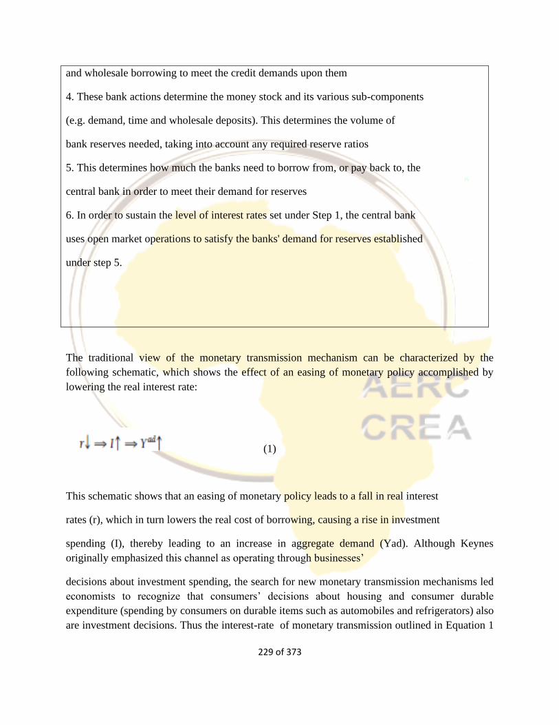
229 of 373

and wholesale borrowing to meet the credit demands upon them

4. These bank actions determine the money stock and its various sub-components

(e.g. demand, time and wholesale deposits). This determines the volume of

bank reserves needed, taking into account any required reserve ratios

5. This determines how much the banks need to borrow from, or pay back to, the

central bank in order to meet their demand for reserves

6. In order to sustain the level of interest rates set under Step 1, the central bank

uses open market operations to satisfy the banks' demand for reserves established

under step 5.

The traditional view of the monetary transmission mechanism can be characterized by the

following schematic, which shows the effect of an easing of monetary policy accomplished by

lowering the real interest rate:

(1)

This schematic shows that an easing of monetary policy leads to a fall in real interest

rates (r), which in turn lowers the real cost of borrowing, causing a rise in investment

spending (I), thereby leading to an increase in aggregate demand (Yad). Although Keynes

originally emphasized this channel as operating through businesses’

decisions about investment spending, the search for new monetary transmission mechanisms led

economists to recognize that consumers’ decisions about housing and consumer durable

expenditure (spending by consumers on durable items such as automobiles and refrigerators) also

are investment decisions. Thus the interest-rate of monetary transmission outlined in Equation 1

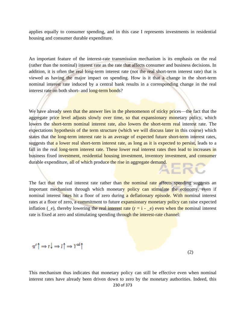
230 of 373

applies equally to consumer spending, and in this case I represents investments in residential

housing and consumer durable expenditure.

An important feature of the interest-rate transmission mechanism is its emphasis on the real

(rather than the nominal) interest rate as the rate that affects consumer and business decisions. In

addition, it is often the real long-term interest rate (not the real short-term interest rate) that is

viewed as having the major impact on spending. How is it that a change in the short-term

nominal interest rate induced by a central bank results in a corresponding change in the real

interest rate on both short- and long-term bonds?

We have already seen that the answer lies in the phenomenon of sticky prices—the fact that the

aggregate price level adjusts slowly over time, so that expansionary monetary policy, which

lowers the short-term nominal interest rate, also lowers the short-term real interest rate. The

expectations hypothesis of the term structure (which we will discuss later in this course) which

states that the long-term interest rate is an average of expected future short-term interest rates,

suggests that a lower real short-term interest rate, as long as it is expected to persist, leads to a

fall in the real long-term interest rate. These lower real interest rates then lead to increases in

business fixed investment, residential housing investment, inventory investment, and consumer

durable expenditure, all of which produce the rise in aggregate demand.

The fact that the real interest rate rather than the nominal rate affects spending suggests an

important mechanism through which monetary policy can stimulate the economy, even if

nominal interest rates hit a floor of zero during a deflationary episode. With nominal interest

rates at a floor of zero, a commitment to future expansionary monetary policy can raise expected

inflation (_e), thereby lowering the real interest rate (r = i - _e) even when the nominal interest

rate is fixed at zero and stimulating spending through the interest-rate channel:

(2)

This mechanism thus indicates that monetary policy can still be effective even when nominal

interest rates have already been driven down to zero by the monetary authorities. Indeed, this

231 of 373

mechanism explains why the Federal Reserve in the USA resorted in December 2008 to the

nonconventional monetary policy of committing to keep the federal funds rate at zero for an

extended period of time. By so doing, the Fed was trying to keep inflation expectations from

falling in order to make sure that real interest rates remained low, so as to stimulate the economy.

In addition, the commitment to keep interest rates low for an extended period of time would help

lower long-term interest rates, which would also induce greater spending.

Some economists, such as John Taylor of Stanford University, take the position that strong

empirical evidence exists for substantial interest-rate effects on consumer and investment

spending through the real cost of borrowing, making the interest-rate monetary transmission

mechanism a strong one. His position is highly controversial, and many researchers, including

Ben Bernanke, former chair of the Fed, and Mark Gertler of New York University, believe that

the empirical evidence does not support strong interest-rate effects that operate through the real

cost of borrowing. Indeed, these researchers see the empirical failure of traditional interest-rate

monetary transmission mechanisms as having provided the stimulus for the search for other

transmission mechanisms of monetary policy.

These other transmission mechanisms fall into two basic categories: those operating through

asset prices other than interest rates, and those operating through asymmetric information effects

on credit markets (the credit view).

Other Asset Price Channels

One drawback of the aggregate demand analysis in previous chapters is that it focuses on only

one asset price, the interest rate, rather than on many asset prices. In addition to bond prices, two

other asset prices receive substantial attention as channels for monetary policy effects: foreign

exchange rates and the prices of equities (stocks).

Exchange Rate Effects on Net Exports With the growing internationalization of economies

throughout the world and the advent of flexible exchange rates, more attention has been paid to

how monetary policy affects exchange rates, which in turn affect net exports and aggregate

demand. The foreign exchange rate channel also involves interest-rate effects because, as we

Will see later, when domestic real interest rates fall, domestic dollar assets become less attractive

relative to assets denominated in foreign currencies. As a result, the value of dollar assets relative

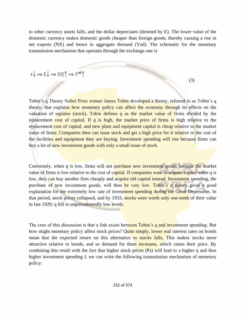
232 of 373

to other currency assets falls, and the dollar depreciates (denoted by E). The lower value of the

domestic currency makes domestic goods cheaper than foreign goods, thereby causing a rise in

net exports (NX) and hence in aggregate demand (Yad). The schematic for the monetary

transmission mechanism that operates through the exchange rate is

(3)

Tobin’s q Theory Nobel Prize winner James Tobin developed a theory, referred to as Tobin’s q

theory, that explains how monetary policy can affect the economy through its effects on the

valuation of equities (stock). Tobin defines q as the market value of firms divided by the

replacement cost of capital. If q is high, the market price of firms is high relative to the

replacement cost of capital, and new plant and equipment capital is cheap relative to the market

value of firms. Companies then can issue stock and get a high price for it relative to the cost of

the facilities and equipment they are buying. Investment spending will rise because firms can

buy a lot of new investment goods with only a small issue of stock.

Conversely, when q is low, firms will not purchase new investment goods because the market

value of firms is low relative to the cost of capital. If companies want to acquire capital when q is

low, they can buy another firm cheaply and acquire old capital instead. Investment spending, the

purchase of new investment goods, will then be very low. Tobin’s q theory gives a good

explanation for the extremely low rate of investment spending during the Great Depression. In

that period, stock prices collapsed, and by 1933, stocks were worth only one-tenth of their value

in late 1929; q fell to unprecedentedly low levels.

The crux of this discussion is that a link exists between Tobin’s q and investment spending. But

how might monetary policy affect stock prices? Quite simply, lower real interest rates on bonds

mean that the expected return on this alternative to stocks falls. This makes stocks more

attractive relative to bonds, and so demand for them increases, which raises their price. By

combining this result with the fact that higher stock prices (Ps) will lead to a higher q and thus

higher investment spending I, we can write the following transmission mechanism of monetary

policy:

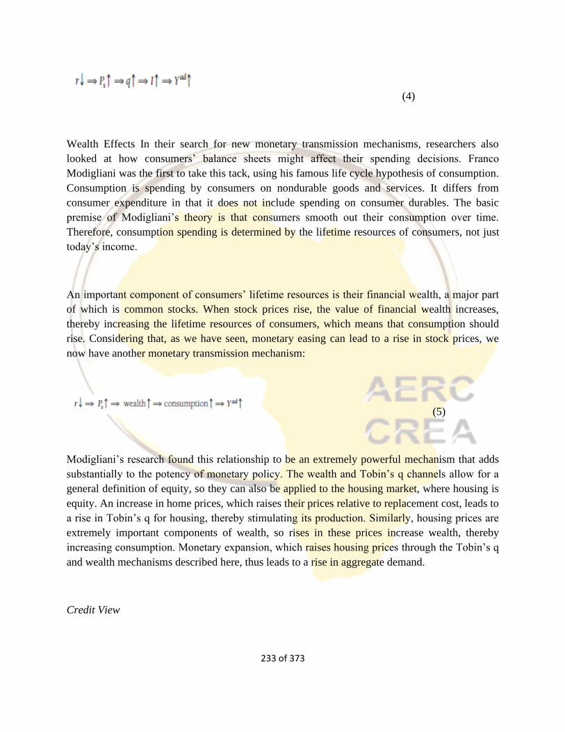
233 of 373

(4)

Wealth Effects In their search for new monetary transmission mechanisms, researchers also

looked at how consumers’ balance sheets might affect their spending decisions. Franco

Modigliani was the first to take this tack, using his famous life cycle hypothesis of consumption.

Consumption is spending by consumers on nondurable goods and services. It differs from

consumer expenditure in that it does not include spending on consumer durables. The basic

premise of Modigliani’s theory is that consumers smooth out their consumption over time.

Therefore, consumption spending is determined by the lifetime resources of consumers, not just

today’s income.

An important component of consumers’ lifetime resources is their financial wealth, a major part

of which is common stocks. When stock prices rise, the value of financial wealth increases,

thereby increasing the lifetime resources of consumers, which means that consumption should

rise. Considering that, as we have seen, monetary easing can lead to a rise in stock prices, we

now have another monetary transmission mechanism:

(5)

Modigliani’s research found this relationship to be an extremely powerful mechanism that adds

substantially to the potency of monetary policy. The wealth and Tobin’s q channels allow for a

general definition of equity, so they can also be applied to the housing market, where housing is

equity. An increase in home prices, which raises their prices relative to replacement cost, leads to

a rise in Tobin’s q for housing, thereby stimulating its production. Similarly, housing prices are

extremely important components of wealth, so rises in these prices increase wealth, thereby

increasing consumption. Monetary expansion, which raises housing prices through the Tobin’s q

and wealth mechanisms described here, thus leads to a rise in aggregate demand.

Credit View

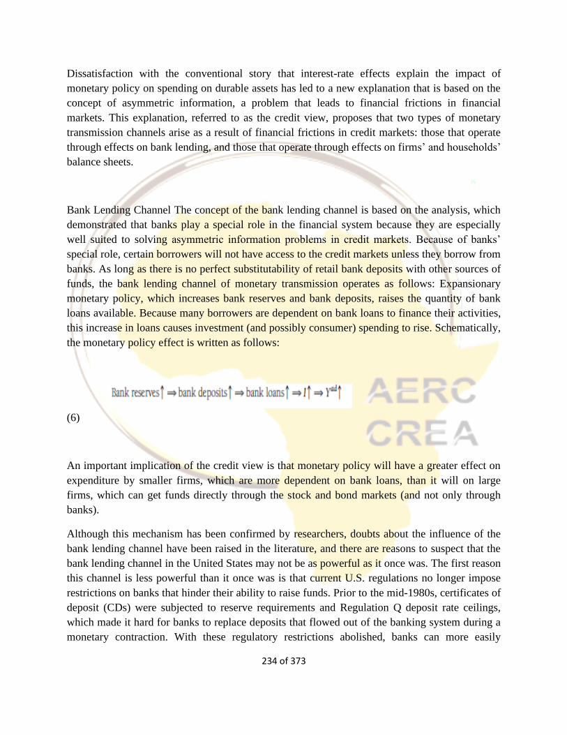
234 of 373

Dissatisfaction with the conventional story that interest-rate effects explain the impact of

monetary policy on spending on durable assets has led to a new explanation that is based on the

concept of asymmetric information, a problem that leads to financial frictions in financial

markets. This explanation, referred to as the credit view, proposes that two types of monetary

transmission channels arise as a result of financial frictions in credit markets: those that operate

through effects on bank lending, and those that operate through effects on firms’ and households’

balance sheets.

Bank Lending Channel The concept of the bank lending channel is based on the analysis, which

demonstrated that banks play a special role in the financial system because they are especially

well suited to solving asymmetric information problems in credit markets. Because of banks’

special role, certain borrowers will not have access to the credit markets unless they borrow from

banks. As long as there is no perfect substitutability of retail bank deposits with other sources of

funds, the bank lending channel of monetary transmission operates as follows: Expansionary

monetary policy, which increases bank reserves and bank deposits, raises the quantity of bank

loans available. Because many borrowers are dependent on bank loans to finance their activities,

this increase in loans causes investment (and possibly consumer) spending to rise. Schematically,

the monetary policy effect is written as follows:

(6)

An important implication of the credit view is that monetary policy will have a greater effect on

expenditure by smaller firms, which are more dependent on bank loans, than it will on large

firms, which can get funds directly through the stock and bond markets (and not only through

banks).

Although this mechanism has been confirmed by researchers, doubts about the influence of the

bank lending channel have been raised in the literature, and there are reasons to suspect that the

bank lending channel in the United States may not be as powerful as it once was. The first reason

this channel is less powerful than it once was is that current U.S. regulations no longer impose

restrictions on banks that hinder their ability to raise funds. Prior to the mid-1980s, certificates of

deposit (CDs) were subjected to reserve requirements and Regulation Q deposit rate ceilings,

which made it hard for banks to replace deposits that flowed out of the banking system during a

monetary contraction. With these regulatory restrictions abolished, banks can more easily

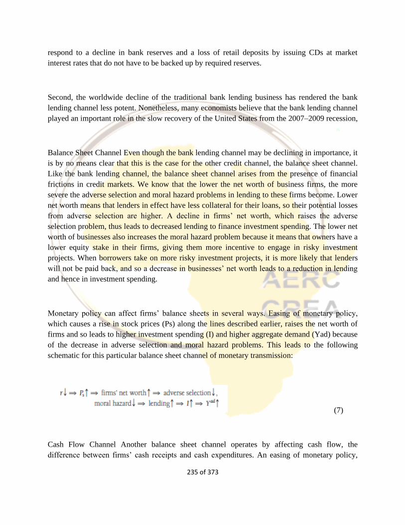
235 of 373

respond to a decline in bank reserves and a loss of retail deposits by issuing CDs at market

interest rates that do not have to be backed up by required reserves.

Second, the worldwide decline of the traditional bank lending business has rendered the bank

lending channel less potent. Nonetheless, many economists believe that the bank lending channel

played an important role in the slow recovery of the United States from the 2007–2009 recession,

Balance Sheet Channel Even though the bank lending channel may be declining in importance, it

is by no means clear that this is the case for the other credit channel, the balance sheet channel.

Like the bank lending channel, the balance sheet channel arises from the presence of financial

frictions in credit markets. We know that the lower the net worth of business firms, the more

severe the adverse selection and moral hazard problems in lending to these firms become. Lower

net worth means that lenders in effect have less collateral for their loans, so their potential losses

from adverse selection are higher. A decline in firms’ net worth, which raises the adverse

selection problem, thus leads to decreased lending to finance investment spending. The lower net

worth of businesses also increases the moral hazard problem because it means that owners have a

lower equity stake in their firms, giving them more incentive to engage in risky investment

projects. When borrowers take on more risky investment projects, it is more likely that lenders

will not be paid back, and so a decrease in businesses’ net worth leads to a reduction in lending

and hence in investment spending.

Monetary policy can affect firms’ balance sheets in several ways. Easing of monetary policy,

which causes a rise in stock prices (Ps) along the lines described earlier, raises the net worth of

firms and so leads to higher investment spending (I) and higher aggregate demand (Yad) because

of the decrease in adverse selection and moral hazard problems. This leads to the following

schematic for this particular balance sheet channel of monetary transmission:

(7)

Cash Flow Channel Another balance sheet channel operates by affecting cash flow, the

difference between firms’ cash receipts and cash expenditures. An easing of monetary policy,

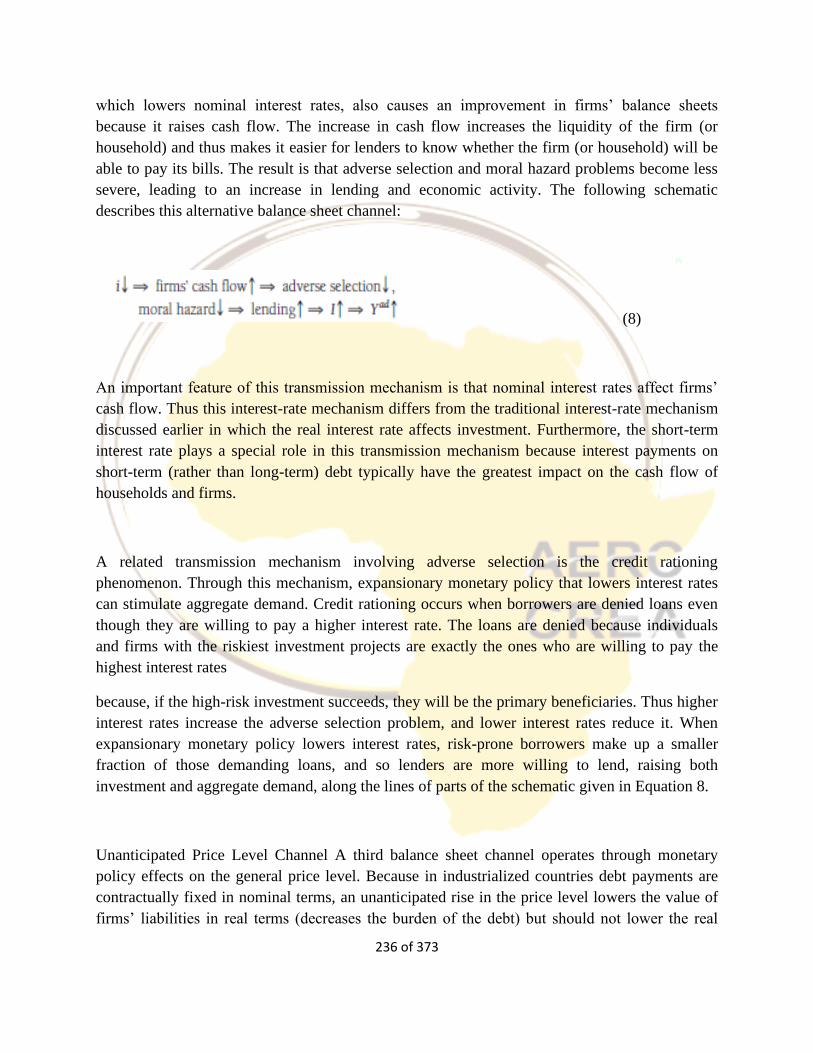
236 of 373

which lowers nominal interest rates, also causes an improvement in firms’ balance sheets

because it raises cash flow. The increase in cash flow increases the liquidity of the firm (or

household) and thus makes it easier for lenders to know whether the firm (or household) will be

able to pay its bills. The result is that adverse selection and moral hazard problems become less

severe, leading to an increase in lending and economic activity. The following schematic

describes this alternative balance sheet channel:

(8)

An important feature of this transmission mechanism is that nominal interest rates affect firms’

cash flow. Thus this interest-rate mechanism differs from the traditional interest-rate mechanism

discussed earlier in which the real interest rate affects investment. Furthermore, the short-term

interest rate plays a special role in this transmission mechanism because interest payments on

short-term (rather than long-term) debt typically have the greatest impact on the cash flow of

households and firms.

A related transmission mechanism involving adverse selection is the credit rationing

phenomenon. Through this mechanism, expansionary monetary policy that lowers interest rates

can stimulate aggregate demand. Credit rationing occurs when borrowers are denied loans even

though they are willing to pay a higher interest rate. The loans are denied because individuals

and firms with the riskiest investment projects are exactly the ones who are willing to pay the

highest interest rates

because, if the high-risk investment succeeds, they will be the primary beneficiaries. Thus higher

interest rates increase the adverse selection problem, and lower interest rates reduce it. When

expansionary monetary policy lowers interest rates, risk-prone borrowers make up a smaller

fraction of those demanding loans, and so lenders are more willing to lend, raising both

investment and aggregate demand, along the lines of parts of the schematic given in Equation 8.

Unanticipated Price Level Channel A third balance sheet channel operates through monetary

policy effects on the general price level. Because in industrialized countries debt payments are

contractually fixed in nominal terms, an unanticipated rise in the price level lowers the value of

firms’ liabilities in real terms (decreases the burden of the debt) but should not lower the real

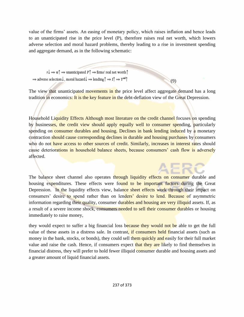
237 of 373

value of the firms’ assets. An easing of monetary policy, which raises inflation and hence leads

to an unanticipated rise in the price level (P), therefore raises real net worth, which lowers

adverse selection and moral hazard problems, thereby leading to a rise in investment spending

and aggregate demand, as in the following schematic:

(9)

The view that unanticipated movements in the price level affect aggregate demand has a long

tradition in economics: It is the key feature in the debt-deflation view of the Great Depression.

Household Liquidity Effects Although most literature on the credit channel focuses on spending

by businesses, the credit view should apply equally well to consumer spending, particularly

spending on consumer durables and housing. Declines in bank lending induced by a monetary

contraction should cause corresponding declines in durable and housing purchases by consumers

who do not have access to other sources of credit. Similarly, increases in interest rates should

cause deteriorations in household balance sheets, because consumers’ cash flow is adversely

affected.

The balance sheet channel also operates through liquidity effects on consumer durable and

housing expenditures. These effects were found to be important factors during the Great

Depression. In the liquidity effects view, balance sheet effects work through their impact on

consumers’ desire to spend rather than on lenders’ desire to lend. Because of asymmetric

information regarding their quality, consumer durables and housing are very illiquid assets. If, as

a result of a severe income shock, consumers needed to sell their consumer durables or housing

immediately to raise money,

they would expect to suffer a big financial loss because they would not be able to get the full

value of these assets in a distress sale. In contrast, if consumers held financial assets (such as

money in the bank, stocks, or bonds), they could sell them quickly and easily for their full market

value and raise the cash. Hence, if consumers expect that they are likely to find themselves in

financial distress, they will prefer to hold fewer illiquid consumer durable and housing assets and

a greater amount of liquid financial assets.

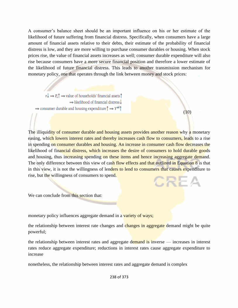
238 of 373

A consumer’s balance sheet should be an important influence on his or her estimate of the

likelihood of future suffering from financial distress. Specifically, when consumers have a large

amount of financial assets relative to their debts, their estimate of the probability of financial

distress is low, and they are more willing to purchase consumer durables or housing. When stock

prices rise, the value of financial assets increases as well; consumer durable expenditure will also

rise because consumers have a more secure financial position and therefore a lower estimate of

the likelihood of future financial distress. This leads to another transmission mechanism for

monetary policy, one that operates through the link between money and stock prices:

(10)

The illiquidity of consumer durable and housing assets provides another reason why a monetary

easing, which lowers interest rates and thereby increases cash flow to consumers, leads to a rise

in spending on consumer durables and housing. An increase in consumer cash flow decreases the

likelihood of financial distress, which increases the desire of consumers to hold durable goods

and housing, thus increasing spending on these items and hence increasing aggregate demand.

The only difference between this view of cash flow effects and that outlined in Equation 8 is that

in this view, it is not the willingness of lenders to lend to consumers that causes expenditure to

rise, but the willingness of consumers to spend.

We can conclude from this section that:

monetary policy influences aggregate demand in a variety of ways;

the relationship between interest rate changes and changes in aggregate demand might be quite

powerful;

the relationship between interest rates and aggregate demand is inverse — increases in interest

rates reduce aggregate expenditure; reductions in interest rates cause aggregate expenditure to

increase

nonetheless, the relationship between interest rates and aggregate demand is complex

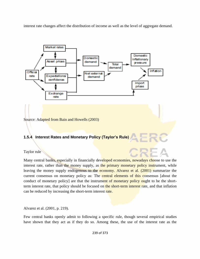
239 of 373

interest rate changes affect the distribution of income as well as the level of aggregate demand.

Source: Adapted from Bain and Howells (2003)

1.5.4 Interest Rates and Monetary Policy (Taylor’s Rule)

Taylor rule

Many central banks, especially in financially developed economies, nowadays choose to use the

interest rate, rather than the money supply, as the primary monetary policy instrument, while

leaving the money supply endogenous to the economy. Alvarez et al. (2001) summarize the

current consensus on monetary policy as: The central elements of this consensus [about the

conduct of monetary policy] are that the instrument of monetary policy ought to be the short-

term interest rate, that policy should be focused on the short-term interest rate, and that inflation

can be reduced by increasing the short-term interest rate.

Alvarez et al. (2001, p. 219).

Few central banks openly admit to following a specific rule, though several empirical studies

have shown that they act as if they do so. Among these, the use of the interest rate as the

240 of 373

operating monetary policy instrument is often espoused in the form of a Taylor rule (Taylor,

1993, 1999), which is:

(1)

where rT is the real interest rate target of the central banks for financial markets, y is real output,

yf is full-employment output, π is the actual inflation rate, πT is the inflation rate desired by the

central bank, and the subscript t refers to period t. πT is called the target inflation rate. Similarly,

yf is the target output level. (yt −yf) is (minus of) the output gap.

The Taylor rule is a feedback rule according to which changes in two indicators, inflation and

output, of the actual performance of the economy cause the central bank to change its real

interest rate target, under this feedback rule, the central bank would increase its target real

interest rate if actual output (or the demand for it) were too high or if inflation were too high,

relative to their long-run or desired levels. Taylor used α = 0.5 and β = 0.5, without estimating

their values. The usual practice now is to specify the Taylor rule with unspecified values for

these parameters, and to estimate them for the country and period being studied. Their relative

ratio should reflect the country’s central bank’s responses, over the sample period, to the output

gap and the deviation of inflation from its desired level.

Since central banks set the nominal rather than the real interest rate, the Taylor rule is also

often written as:

(2)

which specifies the nominal interest rate R set by the central bank. The objective of the

manipulation of the interest rate by the Taylor rule is to engineer inflation and output back to

241 of 373

their target levels and to do so through a gradual adjustment pattern. By implication, under the

Taylor rule, monetary policy is not used to respond to shocks to the macroeconomy that do not

affect the output gap and the deviation of inflation from its desired level, so that this rule limits

the goals of the central bank to the output gap and inflation.

The principle that the monetary authorities should raise nominal interest rates by more than the

increase in the inflation rate has been named the Taylor principle, and it is critical to the success

of monetary policy. Suppose that the Taylor principle is not followed and that the rise in nominal

rates is less than the rise in the inflation rate, so that real interest rates fall when inflation rises.

Serious instability then results, because a rise in inflation leads to an effective easing of monetary

policy, which then leads to even higher inflation in the future. Indeed, this scenario characterizes

the monetary policy of the 1970s, which led to a loss of the nominal anchor and the era of the so-

called “Great Inflation,” when inflation rates climbed to double-digit levels. Fortunately, since

1979, the Taylor principle has become a feature of monetary policy, with much happier

outcomes on both the inflation and aggregate output fronts.

Implicit in the Taylor rule are the following propositions about the usual links between the

interest rate, output and inflation:

An increase in the real interest rate reduces aggregate demand, which reduces inflation, so that

the real interest rate and inflation are negatively related.

There is a close positive relationship between output and inflation. Given the structure of most

economies, there is usually a low positive inflation rate (say, πnairu) when output is at its full-

employment level; inflation rises above πnairu as output rises above its full-employment level

and falls below πnairu as output falls below that level

The preceding version of the Taylor rule is a contemporaneous one, in which the current interest

rate varies with the current output gap and the “inflation gap,” with the latter defined as (πt −

πT). There are at least three other versions of the Taylor rule in the literature. These include a

242 of 373

backward-looking (forward-looking) rule in which the current interest rate is set on the basis of

past (future) values of the output and inflation gaps. A fourth version derives the Taylor rule

from the optimization of a loss function of the central bank. These versions are spelled out in

Chapter 15 on the Keynesian paradigm since its current variant (the new Keynesian model)

incorporates the Taylor rule.

Note that in the long run yt =yf and πt =πT, rT t =r0, so that r0 has to equal the long-run real

interest rate of the economy. Otherwise, the divergence between the real interest rate set by the

central bank and the economy’s real interest rate would cause long-run disequilibrium in the

financial markets of the economy, with consequences for the markets for commodities and labor,

so that neither yf nor πT would be achieved.

In terms of empirical evidence, some form28 of the Taylor rule has often done quite well as the

central bank’s explicit or implicit reaction function for developed, free market economies (Sims,

2001). To cite just one empirical study, Clarida et al. (1998) estimate the monetary policy rules

for France, Germany, Italy, Japan, the UK and the USA. Using a forward looking version of

Taylor’s rule, they report that the central banks of Germany, Japan and the USA can be

implicitly taken to have followed inflation targeting and output stabilization functions.30

An issue actively pursued in further research on the Taylor rule has been whether or not asset

prices and exchange rates should be included in this rule. The argument in favor of their

inclusion is that shifts in them can change aggregate demand. However, some part of these shifts

are often the result of changes in output and inflation, so that only the impact of their residual

shifts on inflation and output would need to be offset through monetary policy. Doing so yields

extended forms of the Taylor rule.

Many empirical studies report that using some form of an augmented Taylor rule, such as

incorporating changes in wealth or house prices or exchange rates, leads to greater stabilization

of the economy. However, none of these extended forms has come into general usage in

macroeconomic modeling, so we choose not to present them or incorporate them into the

analysis of this chapter. The Taylor rule is re-examined

Integration of the interest rate as the operating monetary target into the macroeconomic model

243 of 373

Our desire in the following analysis is to develop a macroeconomic model that has the simplicity

of the IS–LM one and is comparable with it. In the IS–LM model, the central bank holds the

money supply constant. The corresponding assumption for the interest rate as the monetary

policy instrument is that the central bank holds the interest rate constant. Therefore, for the

following analysis, we adopt the assumption that the central bank sets the real interest rate at a

fixed level, rT, which we designate as the “target rate,” and formulate the macroeconomic model

under this assumption. This model can be used to analyze the impact of changes in this interest

rate, irrespective of whether the changes are made on a discretionary basis or according to a rule

such as the Taylor rule.

The assumption made on monetary policy is that the central bank successfully targets and sets

the economy’s real interest rate r at r0. That is, under this simple targeting policy,

(4)

Plotting this interest rate in the (r, y) space of the IS diagram, we have a horizontal line at the

target real interest rate. This is shown in Figure 5.11 by the “interest rate target curve” labeled

IRT. An alternative to the above assumption of a simple fixed interest rate rule is a simple

feedback rule such as:

(5)

(2) can also be modified to a Taylor-type rule but with targeting of price level, rather than

inflation, as in:

(6)

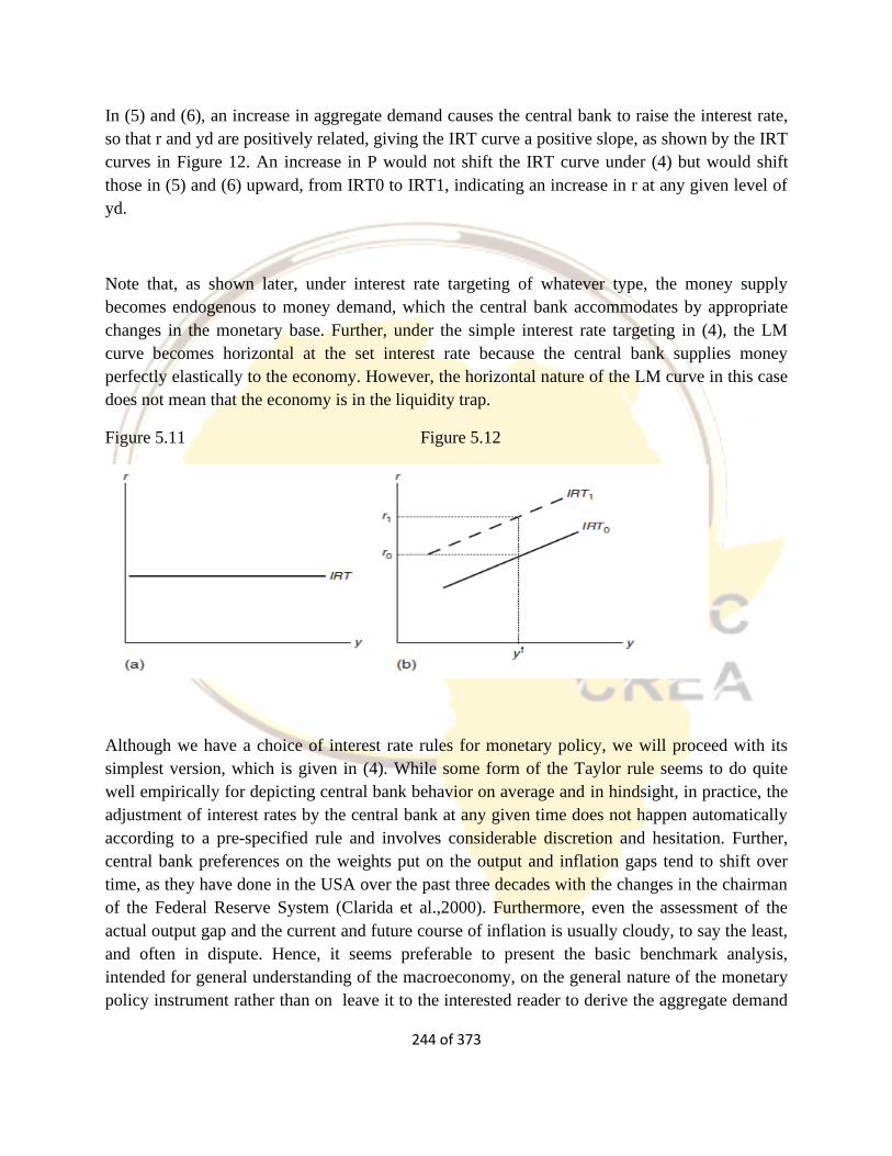
244 of 373

In (5) and (6), an increase in aggregate demand causes the central bank to raise the interest rate,

so that r and yd are positively related, giving the IRT curve a positive slope, as shown by the IRT

curves in Figure 12. An increase in P would not shift the IRT curve under (4) but would shift

those in (5) and (6) upward, from IRT0 to IRT1, indicating an increase in r at any given level of

yd.

Note that, as shown later, under interest rate targeting of whatever type, the money supply

becomes endogenous to money demand, which the central bank accommodates by appropriate

changes in the monetary base. Further, under the simple interest rate targeting in (4), the LM

curve becomes horizontal at the set interest rate because the central bank supplies money

perfectly elastically to the economy. However, the horizontal nature of the LM curve in this case

does not mean that the economy is in the liquidity trap.

Figure 5.11 Figure 5.12

Although we have a choice of interest rate rules for monetary policy, we will proceed with its

simplest version, which is given in (4). While some form of the Taylor rule seems to do quite

well empirically for depicting central bank behavior on average and in hindsight, in practice, the

adjustment of interest rates by the central bank at any given time does not happen automatically

according to a pre-specified rule and involves considerable discretion and hesitation. Further,

central bank preferences on the weights put on the output and inflation gaps tend to shift over

time, as they have done in the USA over the past three decades with the changes in the chairman

of the Federal Reserve System (Clarida et al.,2000). Furthermore, even the assessment of the

actual output gap and the current and future course of inflation is usually cloudy, to say the least,

and often in dispute. Hence, it seems preferable to present the basic benchmark analysis,

intended for general understanding of the macroeconomy, on the general nature of the monetary

policy instrument rather than on leave it to the interested reader to derive the aggregate demand

245 of 373

functions under (5) and (6) – or one of the other forms of the Taylor rule, some more of which

are specified in

1.5.5 Theories of Central Bank Independence and Time Consistency of Policies

This section focuses on the analytical treatment of three major issues: independence of the

central bank and time consistency of policies. Assuming a potential for tradeoffs among goals,

this chapter examines the determination of the choices made and the potential for conflicts

among the monetary and fiscal authorities. This discussion leads to the examination of the

independence of central banks from governments and legislatures.

I shall also introduce you to the superiority of intertemporal optimization policies to myopic

ones, which can have an inflationary bias. Intertemporal optimization over time provides two

types of policy approaches. One of these is the time-consistent one in which the policy path for

the current and future periods is derived only once and followed for all future periods. The

second approach allows reoptimization every period with an unchanging objective function.

In cases of such conflicts, the ability of the central bank to pursue its own choices becomes

important and is discussed under the heading of the independence of the central bank. The other

two major issues addressed in this section are those of the time consistency and credibility of

policies. The time consistency of monetary policies deals with the question of whether the

central bank should determine its policies for the future periods within its horizon and stick to

them, or should retain discretion to reformulate its policies as time passes. Discretionary policies

can be arbitrary ones, be derived from one-period (“myopic”) optimization or be based on

continual intertemporal reoptimization as each period passes.

Choosing Among Multiple Goals

As discussed in the last chapter, economic theory and central bank beliefs prior to the 1980s had

indicated that several goals could be addressed through monetary policy. For the analysis of such

a possibility, this section assumes that the central bank has a multiplicity of goals. Focusing only

on the primary goals, the instruments available for achieving the multiple goals are severely

246 of 373

limited in number and scope so that not all the goals can be attained through the use of monetary

policy. Therefore, the central bank has to make a choice among its desired goals or combinations

of them.

Assume that the central bank’s preferences over the goal variables are consistent and transitive,

so that there exists an ordinal utility function over the goal variables. For diagrammatic analysis,

the indifference curves between any given pair of these variables can be derived from this utility

function.

Choosing between inflation and unemployment

The goal variables of many central banks include the rate of inflation and the unemployment

rate, which can be a goal variable in its own right or a proxy for the output gap. Assume that the

central bank’s preferences over these variables can be encompassed in an objective/utility

function of the form:

U = U(π, u) (1)

where π is the rate of inflation, u is the rate of unemployment, and Uπ ,Uu < 0. Hence, the

indifference curves in the (π, u) space are negatively sloped. Further, it is reasonable to assume

that the undesirability – that is, disutility – of each variable keeps on increasing, ceteris paribus,

with higher levels of it, so that Uππ,Uuu < 0. Hence, as the rate of inflation rises, the central

bank is willing to accept a higher marginal increase in the unemployment rate in order to prevent

a further rise in the rate of inflation, so that the indifference or tradeoff curves between the rates

of inflation have the usual convex shape, as shown in Figure 5.13 by the curves ICB and I_CB.

A host of such curves exist, with a curve passing through every

Figure 5.13

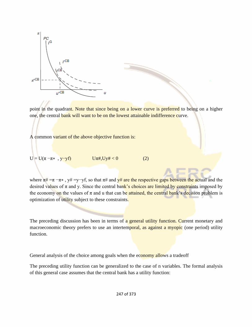
247 of 373

point in the quadrant. Note that since being on a lower curve is preferred to being on a higher

one, the central bank will want to be on the lowest attainable indifference curve.

A common variant of the above objective function is:

U = U(π −π∗ , y−yf) Uπ#,Uy# < 0 (2)

where π# =π −π∗ , y# =y−yf, so that π# and y# are the respective gaps between the actual and the

desired values of π and y. Since the central bank’s choices are limited by constraints imposed by

the economy on the values of π and u that can be attained, the central bank’s decision problem is

optimization of utility subject to these constraints.

The preceding discussion has been in terms of a general utility function. Current monetary and

macroeconomic theory prefers to use an intertemporal, as against a myopic (one period) utility

function.

General analysis of the choice among goals when the economy allows a tradeoff

The preceding utility function can be generalized to the case of n variables. The formal analysis

of this general case assumes that the central bank has a utility function:

248 of 373

U = U(x1, . . ., xn) (3)

At this stage, we assume that the central bank’s choice is subject to only one constraint, which

has the form:

f (x1, . . ., xn; z,Ψ ) = 0 (4)

where:

xi = ith goal variable

z = vector of instruments available to the central bank

Ψ = vector of exogenous variables.

The goal variables can be levels of variables, their growth rates or even such variables as the

output gap and the “inflation gap,” where the gaps are deviations from their desired levels. U(.)

represents the central bank’s preferences over its goals. These depend upon the organizational

structure of the central bank, the interactions between the policy makers, their perceptions of

society’s goals, the structure of the economy and of what is achievable, political pressures, and

so on. Equation (4) should properly specify the actual form of the constraint. However, this form

is usually not known, so that the form of the constraint used by the central bank is that perceived

by it and is based on its knowledge of the structure of the economy and the political and social

environment. However, under imperfect information on the economy, the relevant constraint

perceived by the central bank may not necessarily or even usually be the actual one imposed by

the economy.1 The central bank is taken to maximize (3) subject to (4) in order to determine its

optimal choices among the goals.

The basic objections to the use of a preference function are to its requirements of consistency and

transitivity in making choices. The central bank’s decisions are made by a host of individuals and

its major choices, if consciously made, are by a group. Such group decisions in a democratic

framework need not necessarily be consistent and transitive, even at a point in time, let alone

over time. Further, the policy makers in the central bank change over time, so that its preferences

are likely to shift over time. Hence, one must be cautious in explaining the choices among goals

249 of 373

made by the central bank within a static utility function and its implied set of indifference curves,

especially when there has been a change in its management.

In spite of these objections, the preceding analysis furnishes considerable insights into the

problem of choice among alternative goals. Empirical and descriptive studies using data up to

the 1980s indicate considerable validity for this analysis and show that the central banks often

manipulated their policy instruments, such as the monetary base and interest rates, in a

systematic fashion to address their chosen goal levels.

Choices under the economy’s supply constraint

There are several forms of the economy’s supply constraint relating u and π. Of these, the

Phillips curve (see in Section 5) was proposed in 1958 by A.W. Phillips and soon began to be

treated as the economy’s constraint between inflation and unemployment. Its general form was:

u = f (π) f ‘< 0 (5)

This constraint allows the central bank to trade between higher inflation and lower

unemployment. Optimization of the utility function (1) subject to (5) yields the optimal values of

π and u, with higher inflation rates yielding lower unemployment. While most Keynesians of the

1960s and 1970s accepted some form of (5) as the economy’s constraint and explained central

banks’ monetary policy under it, many economists, especially neoclassical ones, believed that

the economy had a vertical Phillips curve for the long run. Their arguments were subsequently

refined by Friedman and Lucaswho asserted that the proper form of the economy’s constraint

was the Friedman–Lucas aggregate supply curve, also known as the expectations-augmented

Phillips curve. This constraint, under the assumption of rational expectations, is of the form:

(u−un) = f (π −Eπ) f ‘< 0 (6)

where du/dEπ= 0 and the use of a systematic monetary policy by the central bank changes both π

and Eπ by the same extent, so that (π−Eπ) would not change. This constraint belongs to the

modern classical approach. According to it, unemployment can only be made to deviate from its

250 of 373

natural rate through unanticipated inflation, which, given rational expectations, requires a

random monetary policy. Therefore, there is no tradeoff between these variables which

systematic monetary policy by the central bank can exploit, so that the recommendation is that

the central bank should adopt the target of price stability. Many central banks adopted this

economic framework in the 1990s and some economists advocated that price stability or a low

rate of inflation should be the central bank’s only goal variable. Further, in the 1990s, many

central banks came to believe that higher rates of inflation have little to contribute in terms of

higher output, while they could lead to escalating inflation and lower output. At the same time,

negative rates of inflation are considered inimical to full employment because of their potential

for causing a recession.

Given these beliefs, the utility-maximizing goal rate of inflation would be zero, or a low

positive inflation rate.

As pointed out earlier, some economists choose to work with the objective function:

U = U(π −π∗ , y−yf) Uπ#,Uy# < 0 (7)

where π# = π−π∗, y# = y−yf, so that π# and y# are the respective gaps between the actual and the

desired values of π and y. Given this objective function, maintaining the expectations-augmented

Phillips curve as the constraint, as well as assuming that the central bank does not want to or

cannot fool the public by causing unanticipated inflation, implies that the optimal values of

inflation and output are π∗ and yf, of which the former can be achieved through systematic

monetary policy. The latter is not affected by monetary policy but is determined by the long-run

performance of the economy.

However, for imperfect competition and price rigidities, the new Keynesians propose a different

form of the supply constraint to (6), so that their policy recommendations would differ from the

above. This form is known as the new Keynesian Phillips curve. The preceding discussion of the

Phillips curve, its expectations-augmented version and the new Keynesian Phillips curve

illustrates that the accurate form of the economy’s constraint is usually not known. There are

continual disputes among economists even about its general form, less alone the specific one

with numerically specified values of the parameters.

251 of 373

Conflicts among policy makers: theoretical analysis

Another application of the utility approach is to the choices exercised by several (at least two)

policy makers over the same set of goal variables. Different policy-making bodies in the

economy are likely to have different preference functions and hence different indifference curves

between any given pair of variables. Therefore, the formal optimization analysis for two policy

makers A and B would be:

For policy maker A:

Maximize UA = UA(x1, . . ., xn) (8)

subject to A’s perceived constraint:

f A(x1, . . ., xn; z, Ψ ) = 0 (10)

For policy maker B:

Maximize UB = UB(x1, . . ., xn) (11)

subject to B’s perceived constraint:

f B(x1, . . ., xn; z, Ψ ) = 0

The superscripts A and B refer to the policy maker. Since both the utility functions and the

perceived constraints can differ, the optimal values of the goals for x1A , . . ., xnA will differ

from x1B , . . ., xnB , so that working at cross purposes can be a common phenomenon, rather

than a rare occurrence, among policy makers in the economy. This possibility depends upon the

differences in the utility functions, becoming reinforced by any differences in the policy makers’

252 of 373

perceptions of the actual present and expected course of the economy. In most cases, such

conflicts in the understanding of the economy and desirable tradeoffs among objectives by the

fiscal and monetary authorities of a given country tend to be mild. However, they can erupt into

open and sometimes acrimonious public debate in times of radical economic and political change

and of differences in ideology.

The two principal tools for the control of aggregate demand are monetary and fiscal policies. In a

country with an independent central bank, monetary policy is in the control of the central bank

whereas fiscal policy is in the hands of the legislature and the government. The latter depends on

the public for electoral support and generally tends to attach greater undesirability to increases in

unemployment relative to increases in inflation than does the central bank which is usually more

vitally concerned with inflation. Formally, in terms of the marginal rates of substitution of the

two policy makers, ∂π/∂uCB <(∂π/∂u)G, where CB stands for the central bank and G for the

government, implying (Figure 12.2) that the indifference curves of the central bank are steeper

than those of the government. This implies that for a given constraint f (π,u) = 0, the central bank

would adopt a monetary policy aimed at achieving a lower rate of inflation than the government.

This is illustrated in Figure 5.13 in which the central bank’s indifference curves are shown by

ICB, the government’s by IG, and the economy’s (common) constraint is shown by PC. The

central bank’s optimal choice is for (π ∗CB, u∗CB) and the government’s is for (π∗G, u∗G),

implying a more expansive stance by the government for the economy relative to that by the

central bank. There therefore exists in this case a conflict between the central bank and the

government on the desired rates of inflation and unemployment for the economy. If each tries to

achieve its goals through the policy at its command, neither will achieve their own goals. Over

time, the political process may bring about a narrow “consensus range” within which the

differences between the central bank and the government over the desired goals are

Figure 5.14

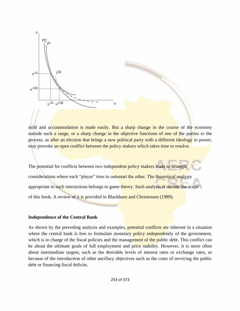
253 of 373

mild and accommodation is made easily. But a sharp change in the course of the economy

outside such a range, or a sharp change in the objective functions of one of the parties to the

process, as after an election that brings a new political party with a different ideology to power,

may provoke an open conflict between the policy makers which takes time to resolve.

The potential for conflicts between two independent policy makers leads to strategic

considerations where each “player” tries to outsmart the other. The theoretical analysis

appropriate to such interactions belongs to game theory. Such analysis is outside the scope

of this book. A review of it is provided in Blackburn and Christensen (1989).

Independence of the Central Bank

As shown by the preceding analysis and examples, potential conflicts are inherent in a situation

where the central bank is free to formulate monetary policy independently of the government,

which is in charge of the fiscal policies and the management of the public debt. This conflict can

be about the ultimate goals of full employment and price stability. However, it is more often

about intermediate targets, such as the desirable levels of interest rates or exchange rates, or

because of the introduction of other ancillary objectives such as the costs of servicing the public

debt or financing fiscal deficits.

254 of 373

While the potential for conflict can be avoided by the subordination of the central bank to the

government, its independence usually ensures lower inflation rates. The USA Fed is now one of

the most independent central banks in the world. In practice, the Bank of Canada has retained its

independence, though there is close consultation between the Governor and the Minister of

Finance on inflation targets and policy changes. The British experiments with its central bank’s

independence have varied over time. While the Bank of England was historically a quasi-private

bank, independent of the government, the dominance of the government over the Bank of

England was legislated by the Bank Act of 1946, which nationalized its ownership. It also

allocated the choice over the goals and targets of monetary policy to the Chancellor of the

Exchequer, representing the government, leaving the Bank of England with a consultative and

implemental role.

The Case for Independence

The strongest argument for an independent central bank rests on the view that subjecting it to

more political pressures would impart an inflationary bias to monetary policy. In the view of

many observers, politicians in a democratic society are shortsighted because they are driven by

the need to win their next election. With this as their primary goal, they are unlikely to focus on

long-run objectives such as promoting a stable price level. Instead, they will seek short-run

solutions to problems such as high unemployment and high interest rates, even if the short-run

solutions have undesirable long-run consequences. For example, we saw earleir that high money

growth can lead initially to a drop in interest rates but might cause an increase later, as inflation

heats up. Would a

Federal Reserve in the USA under the control of Congress or the president be more likely to

pursue a policy of excessive money growth when interest rates are high, even though such a

policy would eventually lead to inflation and even higher interest rates in the future? The

advocates of an independent Federal Reserve say yes. They believe that a politically insulated

Fed is more likely to be concerned with long-run objectives and thus more likely to defend a

sound dollar and a stable price level.

A variation on the preceding argument is that the political process in America could lead to a

political business cycle, in which just before an election, expansionary policies are pursued to

lower unemployment and interest rates. After the election, the bad effects of these policies—high

255 of 373

inflation and high interest rates—come home to roost, requiring contractionary policies that

politicians hope the public will forget before the next election. There is some evidence that such

a political business cycle exists in the United States, and a Federal Reserve under the control of

Congress or the president might make the cycle even more pronounced.

Another argument for central bank independence is that control of monetary policy is too

important to be left to politicians, a group that has repeatedly demonstrated a lack of expertise at

making hard decisions on issues of great economic importance, such as reducing the budget

deficit or reforming the banking system.

Both the CB and politicians are agents of the public (the principals), and both politicians and the

CB have incentives to act in their own interest rather than in the interest of the public. The

argument supporting Federal Reserve independence is that the principal–agent problem is worse

for politicians than for the Fed because politicians have fewer incentives to act in the public

interest.

Indeed, some politicians prefer an independent Fed because it can be used as a public “whipping

boy” to take some of the heat off their backs. It is possible that a politician who in private

opposes an inflationary monetary policy will be forced to support such a policy in public for fear

of not being reelected. An independent Fed can pursue policies that are politically unpopular yet

ultimately in the public interest.

The Case Against Independence

Proponents of a Fed under the control of the president or Congress argue that it is undemocratic

to have monetary policy (which affects almost everyone in the economy) controlled by an elite

group responsible to no one. The current lack of accountability in CBs has serious consequences:

If the Fed performs badly, no provision is in place for replacing members (as there is with

politicians). True, the CB needs to pursue long-run objectives, but elected officials of Congress

vote on long-run issues also (foreign policy, for example). If we push the argument further that

policy is always performed better by elite groups like the Fed, we end up with such conclusions

as “the Joint Chiefs of Staff should determine military budgets” or “the IRS should set tax

policies with no oversight by the president or Congress.” Would you advocate this degree of

independence for the Joint Chiefs or the IRS?

256 of 373

The public holds the president and Congress responsible for the economic well-being of the

country, yet it lacks control over the government agency that may well be the most important

factor in determining the health of the economy. In addition, to achieve a cohesive program that

will promote economic stability, monetary policy must be coordinated with fiscal policy (the

management of government spending and taxation). Only by placing monetary policy under the

control of the politicians who also control fiscal policy can these two policies be prevented from

working at cross-purposes.

Another argument against Federal Reserve independence is that, historically, an independent Fed

has not always used its freedom successfully. The Fed failed miserably in its stated role as lender

of last resort during the Great Depression, and its independence certainly didn’t prevent it from

pursuing an overly expansionary monetary policy in the 1960s and 1970s that contributed to

rapid inflation in this period.

Development Strategies in LDCs, Financing Fiscal Deficits and Central Bank

Independence

The issue of central bank independence takes on another dimension in countries that incur large

and persistent deficits but do not possess adequate capital markets to finance them through new

issues of public debt, and need the central bank to do so through an expansion of the monetary

base. This often happens during wars, even in the developed economies, buthas occurred most

noticeably in recent decades in the LDCs.

LDCs tend to have low output per capita and are not able to raise adequate tax revenue for their

desired levels of public expenditures. The latter are in many countries swollen by their plans for

public development projects or the deficits of their public sector undertakings.

Further, their domestic financial markets are under-developed and cannot support much, if any,

government borrowing, and their ability to borrow abroad is also severely limited. As a result,

many LDCs resort to increases in the monetary base, either directly or indirectly through the

compulsory sale of government bonds to the central bank. This process requires the subservience

of the central bank and its policies to the fiscal needs of the government, and destroys the central

bank’s independent control over monetary policy.

257 of 373

Whether such an arrangement is advantageous to the economy is in considerable doubt. On the

positive side is the financing of public projects that would otherwise not have been financed, or

provision for social objectives such as health, education and alleviation of poverty. On the

negative side is the subordination of increases in the monetary base to budget deficits, with the

consequent loss in control by the central bank over monetary policy and over aggregate demand

and inflation in the economy. From the perspective of price stability, this loss of independent

control of the monetary base by the central bank severely limits its capacity to control inflation.

Many empirical studies have documented that countries with independent central banks, which

are not necessarily obliged to finance the budget deficits, tend to have lower rates of inflation.

Another negative aspect of this arrangement is that the borrowing for the public projects thus

financed is not done in competitive markets at market determined rates. Hence, allocative

efficiency suffers and private projects that could be more efficient and could have been

undertaken are crowded out. These efficiency losses could be considerable and, in the opinion of

many economists, have contributed to the low growth of those LDCs that resorted heavily in the

past to the financing of governmental deficits by increases in the monetary base.

While few central banks in developing countries were effectively independent of the government

prior to the 1990s, the economic arguments and evidence supporting independence have since

then led many developing countries to grant much greater independence to their central banks.

Time Consistency of Policies

The proper design of monetary policies4 over time requires that the central bank have an

intertemporal objective function to rank alternative policies and know the economy’s constraints,

as well as possess knowledge of the current and future responses of the economy to its policies

and how it intends to set its policies in the future.

A time-consistent policy path is one that is derived from optimizing an intertemporal objective

function subject to the appropriate constraints describing the behavior of the economy, with the

optimal policy path over time derived once-for-all and followed as time passes. The latter

requires a commitment to pursue the derived set of policies, both in the current and future

periods, so that the central bank would have to resist the temptation and the political pressures to

deviate from this path. Hence, time consistency of policies is related to the issues of the

258 of 373

independence of the central bank and of a commitment regime under which the central bank will

maintain a pre-set future policy path.

To illustrate, suppose that the central bank does want to pursue time-consistent policies with the

long-term goal of price stability, while the government has the objective of getting re-elected

which, given a short-run Phillips curve tradeoff between inflation and unemployment, is

enhanced by short-term inflationary monetary policies. The central bank is more likely to resist

pressure from the government if it is independent of the political process. Therefore, the

independence of the central bank from the government and the legislature improves its ability to

pursue time-consistent policies. This reasoning is now widely accepted, so that, as pointed out

earlier, the central banks of most developed countries and of many emerging ones now possess a

high degree of independence of the

government.

Time-consistent policies are generally compared with discretionary policies. Discretionary

policies allow the central bank discretion to deviate or not from the pre-set policy path. Under

them, the central bank retains the right to pursue policies as it thinks fit at the time the policies

are pursued. The set of policy types is:

1 Purely arbitrary policies.

2 Myopic (one period) policies. These are derived from myopic (short-term, usually one period)

optimization with short-term goals subject to the constraints for the current period only and with

expectations taken as exogenously given. Further, under this procedure, the policy maker does

not give any advance commitment, even on maintaining the objective function, on its future

policies.

3 (Intertemporal) reoptimization policies. These policies are derived from intertemporal

reoptimization each period for that period and future ones, with an unchanged intertemporal

objective function, which is maximized subject to the long-run or multiperiod constraints

specified by the structure of the economy. Under this procedure, the policy maker gives a

commitment to maintain the same intertemporal objective function over time, but the relevant

constraints can shift with the passage of time. The optimal policy is followed only for the

optimizing period, since the following period’s policy will be the outcome of that period’s

259 of 373

optimization process. Policies of this type are labeled “reoptimization policies” in this chapter

and are the outcome of a dynamic reoptimization process performed each period, but the optimal

policy is followed for the optimizing period only.

4 (Intertemporal) time-consistent policies. These policies are derived from once-forall

intertemporal optimization, with an intertemporal objective function over goals, maximized

subject to the long-run or multi-period constraints specified by the structure of the economy. The

policy path, once derived, is followed in the initial (i.e. optimization period) and all future

periods, so that the optimization exercise is done only in the initial period. If the initial period

has already passed, optimization is not undertaken in the current period. There is clearly an

implicit or explicit commitment to stick to the policy path derived in the initial period. Compared

with the reoptimization procedure, which requires reoptimization each period, time-consistent

policies are derived from just one optimization. Note also that the time consistent optimal policy

path (i.e. under once-for-all optimization) does not imply unchanged or identical policies for

each period since the period constraints can differ, as, for instance, because of foreseen business

cycle fluctuations.

Policies of types 1 to 3 are usually classified as discretionary since the policy maker does not

make a prior commitment to following pre-announced policies for future periods. However, note

that “reoptimization policies” are not arbitrary or myopic, and are discretionary only in the very

limited sense that the policy maker changes the policy pursued from one period to the next only

if the intertemporal reoptimization, with an unchanged objective function, implies such a change.

Contributions in the 1970s and 1980s on the proper design of policies showed that policies

conducted on an arbitrary or myopic basis generally result in poor long-term outcomes. In

particular, relying on a one-period Phillips curve tradeoff between output or unemployment and

inflation, expansionary policies to boost output above its sustainable level would not keep output

on average above its long-run level but would generate inflation, possibly accelerating inflation,

on a continuing basis. This result is known as the inflationary bias of myopic, discretionary

policies. Over time, this realization would sooner or later lead to the reversal of such policies, so

that they would be “time inconsistent.”

Time-consistent and reoptimization policies are clearly preferable to arbitrary policies. From the

perspective of sustainable long-run goals, they are also preferable to myopic policies. However,

it is not clear whether time-consistent policies are also superior to reoptimization policies.

Offhand, the intuitive presumption is that the reoptimization policy procedure is preferable since

it maintains continuous policy flexibility and since, with reoptimization at the beginning of each

period, it eliminates from decision-making what is gone and past – a procedure common in

260 of 373

economics. However, this intuitive presumption was called into question by Kydland and

Prescott (1977). The discussion below is based on their analysis on the optimality of time-

consistent policies relative to reoptimization policies.

1.5.6 Theoretical modelling of the role of Central Banks and monetary policy: The

Three Equation Model of Monetary Policy

This theoretical model is based on the simple New Keynesian in its 3-equation structure and its

modelling of a forward-looking optimizing central bank8. A significant problem for most

students in the more formal versions of the New Keynesian model is the assumption that both

households (in the IS equation) and price-setting firms (in the Phillips curve) are forward

looking. Our approach focuses just on a forward-looking Central Bank (in the Monetary or

Taylor Rule) but does not incorporate forward-looking behavour in either the IS curve or the

Phillips curve.

In this section, we set out the Carlin–Soskice (C-S) simplified version of the 3-equation model to

show how the central bank’s problem-solving can be illustrated algebraically and in a diagram.

We set out to answer the following questions:

How the CB responds to shocks to the economy?

What is it the CB trying to achieve? (CB’s preferences or reaction function)

What prevents the CB to achieve its target? (CB’s constraints)

How does the CB translate its objectives into monetary policy? (Monetary rule)

8This section is based on a section of Carlin and Soskice (2005).

261 of 373

Note that there are two approaches to this – mathematical and diagrammatical approaches. We

will start with the mathematical approach by using the active rule-based monetary policy (MP):

best response interest ® to achieve inflation target. The following are the steps in deriving CB

Monetary Rule (MR) to shock :

Define the central bank’s preferences in terms of deviations from inflation target and equilibrium

output.

Define the central bank’s constraints from the supply side, ie the Phillips Curve (PC)

Derive the best response monetary rule in the output-inflation space, which gives the MR curve.

Once the optimal output-inflation combination is determined using the MR, the central bank uses

the IS curve to implement its choice (by setting the interest rate).

The 3 equations are the IS equation y1 = A−αr0 in which real income y is a positive function of

autonomous expenditure A and a negative function of the real interest rate r; the Phillips curve

π1 = π0 + α (y1 − ye),

where π is the rate of inflation and ye, equilibrium output; and the central bank’s Monetary Rule.

Equilibrium output is the level of output associated with constant inflation. In a world of

imperfect competition, it reflects the mark-up and structural features of the labour market and

welfare state.

We shall see that in order to make its interest rate decision, an optimizing central bank must take

into account the lag in the effect of a change in the interest rate on output — the so-called policy

lag — and any lag in the Phillips curve from a change in output to inflation. The key lags in the

system relevant to the central bank’s interest rate decision are shown in Figure 5.15. In the IS

curve, the choice of interest rate in period zero r0 will only affect output next period y1 as it

takes time for interest rate changes to feed through to expenditure decisions. In the Phillips

curve, this period’s inflation π1 is affected by the current output gap y1−ye and by last period’s

inflation

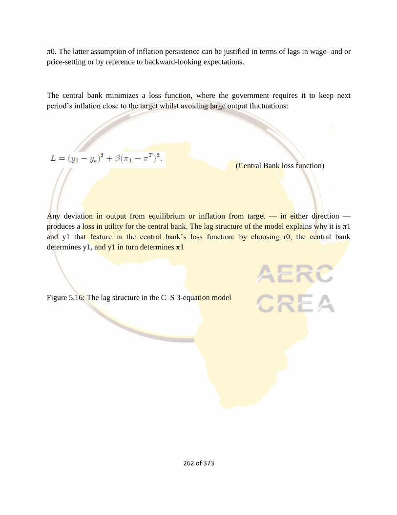
262 of 373

π0. The latter assumption of inflation persistence can be justified in terms of lags in wage- and or

price-setting or by reference to backward-looking expectations.

The central bank minimizes a loss function, where the government requires it to keep next

period’s inflation close to the target whilst avoiding large output fluctuations:

(Central Bank loss function)

Any deviation in output from equilibrium or inflation from target — in either direction —

produces a loss in utility for the central bank. The lag structure of the model explains why it is π1

and y1 that feature in the central bank’s loss function: by choosing r0, the central bank

determines y1, and y1 in turn determines π1

Figure 5.16: The lag structure in the C–S 3-equation model

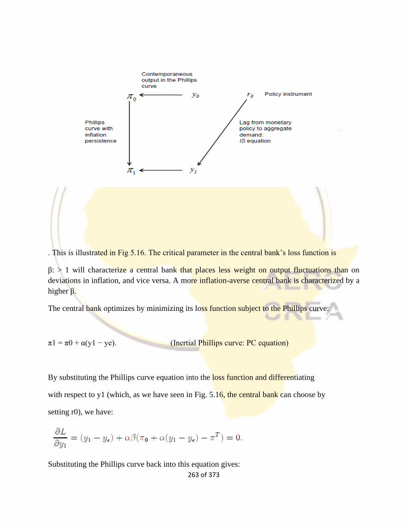
263 of 373

. This is illustrated in Fig 5.16. The critical parameter in the central bank’s loss function is

β: > 1 will characterize a central bank that places less weight on output fluctuations than on

deviations in inflation, and vice versa. A more inflation-averse central bank is characterized by a

higher β.

The central bank optimizes by minimizing its loss function subject to the Phillips curve:

π1 = π0 + α(y1 − ye). (Inertial Phillips curve: PC equation)

By substituting the Phillips curve equation into the loss function and differentiating

with respect to y1 (which, as we have seen in Fig. 5.16, the central bank can choose by

setting r0), we have:

Substituting the Phillips curve back into this equation gives:

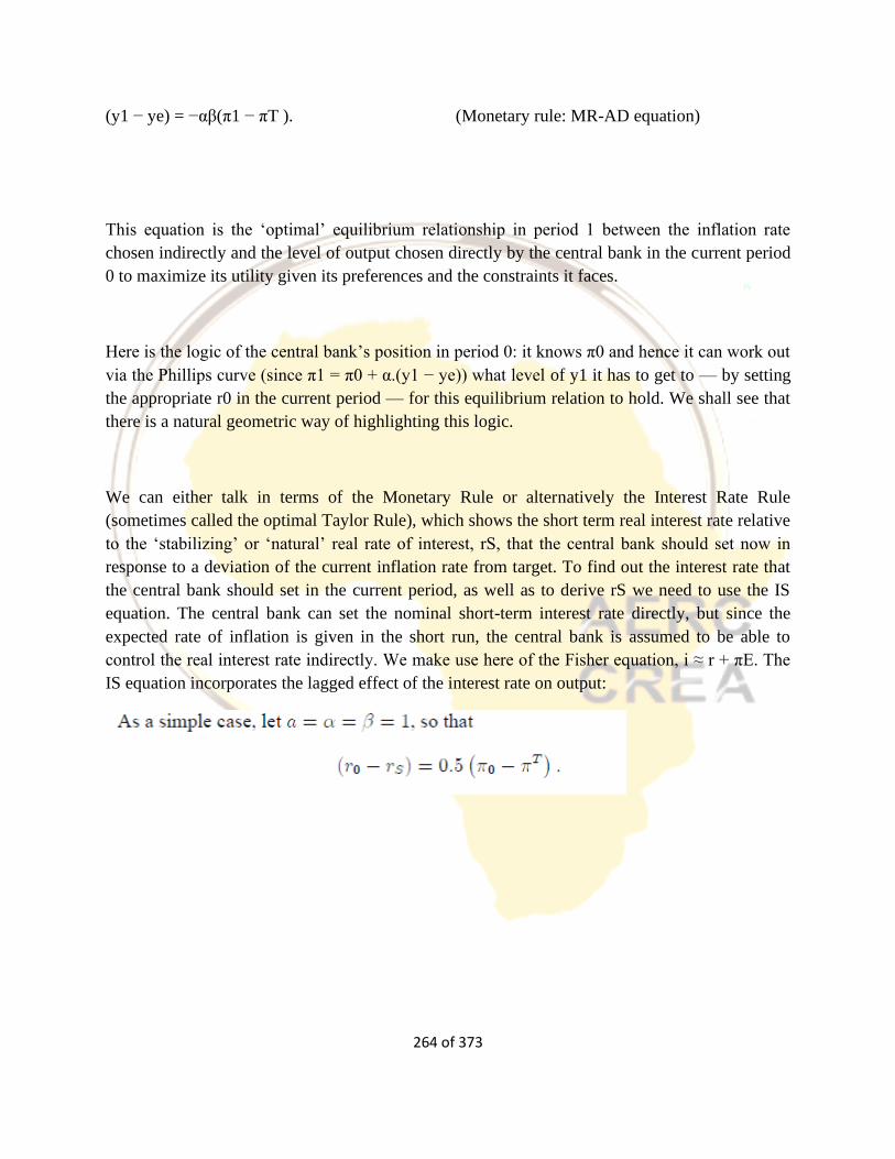
264 of 373

(y1 − ye) = −αβ(π1 − πT ). (Monetary rule: MR-AD equation)

This equation is the ‘optimal’ equilibrium relationship in period 1 between the inflation rate

chosen indirectly and the level of output chosen directly by the central bank in the current period

0 to maximize its utility given its preferences and the constraints it faces.

Here is the logic of the central bank’s position in period 0: it knows π0 and hence it can work out

via the Phillips curve (since π1 = π0 + α.(y1 − ye)) what level of y1 it has to get to — by setting

the appropriate r0 in the current period — for this equilibrium relation to hold. We shall see that

there is a natural geometric way of highlighting this logic.

We can either talk in terms of the Monetary Rule or alternatively the Interest Rate Rule

(sometimes called the optimal Taylor Rule), which shows the short term real interest rate relative

to the ‘stabilizing’ or ‘natural’ real rate of interest, rS, that the central bank should set now in

response to a deviation of the current inflation rate from target. To find out the interest rate that

the central bank should set in the current period, as well as to derive rS we need to use the IS

equation. The central bank can set the nominal short-term interest rate directly, but since the

expected rate of inflation is given in the short run, the central bank is assumed to be able to

control the real interest rate indirectly. We make use here of the Fisher equation, i ≈ r + πE. The

IS equation incorporates the lagged effect of the interest rate on output:

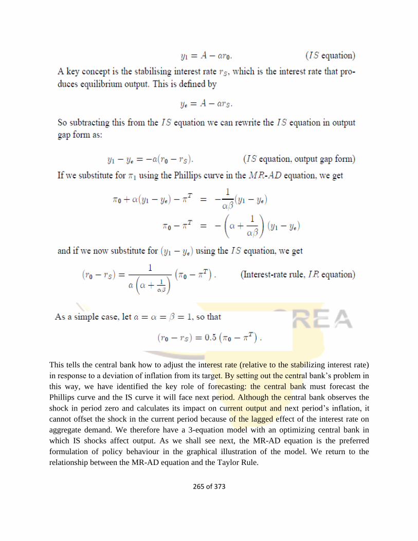
265 of 373

This tells the central bank how to adjust the interest rate (relative to the stabilizing interest rate)

in response to a deviation of inflation from its target. By setting out the central bank’s problem in

this way, we have identified the key role of forecasting: the central bank must forecast the

Phillips curve and the IS curve it will face next period. Although the central bank observes the

shock in period zero and calculates its impact on current output and next period’s inflation, it

cannot offset the shock in the current period because of the lagged effect of the interest rate on

aggregate demand. We therefore have a 3-equation model with an optimizing central bank in

which IS shocks affect output. As we shall see next, the MR-AD equation is the preferred

formulation of policy behaviour in the graphical illustration of the model. We return to the

relationship between the MR-AD equation and the Taylor Rule.

266 of 373

Diagram: the example of an IS shock

We shall now explain how the 3-equation model can be set out in a diagram. A graphical

approach is useful in bringing out the economic intuition at the heart of the model. It allows

students to work through the forecasting exercise of the central bank and to follow the

adjustment process as the optimal monetary policy is implemented.

The first step is to present two of the equations of the 3-equation model. In the lower part of Fig.

2, the vertical Phillips curve at the equilibrium output level, ye, is shown. We think of labour and

product markets as being imperfectly competitive so that the equilibrium output level is where

both wage- and price-setters make no attempt to change the prevailing real wage or relative

prices. Each Phillips curve is indexed by the pre-existing or inertial rate of inflation, πI = π−1. As

shown in Figure 5.17, the economy is in a constant inflation equilibrium at the output level of ye;

inflation is constant at the target rate of πT. Figure 5.17 shows the IS equation in the upper panel:

the stabilizing interest rate, rS, will produce a level of aggregate demand equal to equilibrium

output, ye. We now need to combine the three elements: IS curve, Phillips curve and the Central

Bank’s loss function to show how the central bank formulates monetary policy. To see the

graphical derivation of the monetary rule equation (labelled MR-AD), it is useful to begin with

an example.

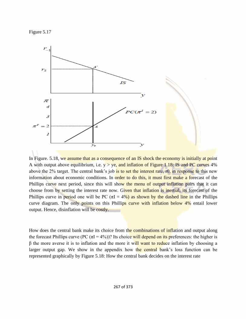
267 of 373

Figure 5.17

In Figure. 5.18, we assume that as a consequence of an IS shock the economy is initially at point

A with output above equilibrium, i.e. y > ye, and inflation of Figure 1.18: IS and PC curves 4%

above the 2% target. The central bank’s job is to set the interest rate, r0, in response to this new

information about economic conditions. In order to do this, it must first make a forecast of the

Phillips curve next period, since this will show the menu of output inflation pairs that it can

choose from by setting the interest rate now. Given that inflation is inertial, its forecast of the

Phillips curve in period one will be PC (πI = 4%) as shown by the dashed line in the Phillips

curve diagram. The only points on this Phillips curve with inflation below 4% entail lower

output. Hence, disinflation will be costly.

How does the central bank make its choice from the combinations of inflation and output along

the forecast Phillips curve (PC (πI = 4%))? Its choice will depend on its preferences: the higher is

β the more averse it is to inflation and the more it will want to reduce inflation by choosing a

larger output gap. We show in the appendix how the central bank’s loss function can be

represented graphically by Figure 5.18: How the central bank decides on the interest rate

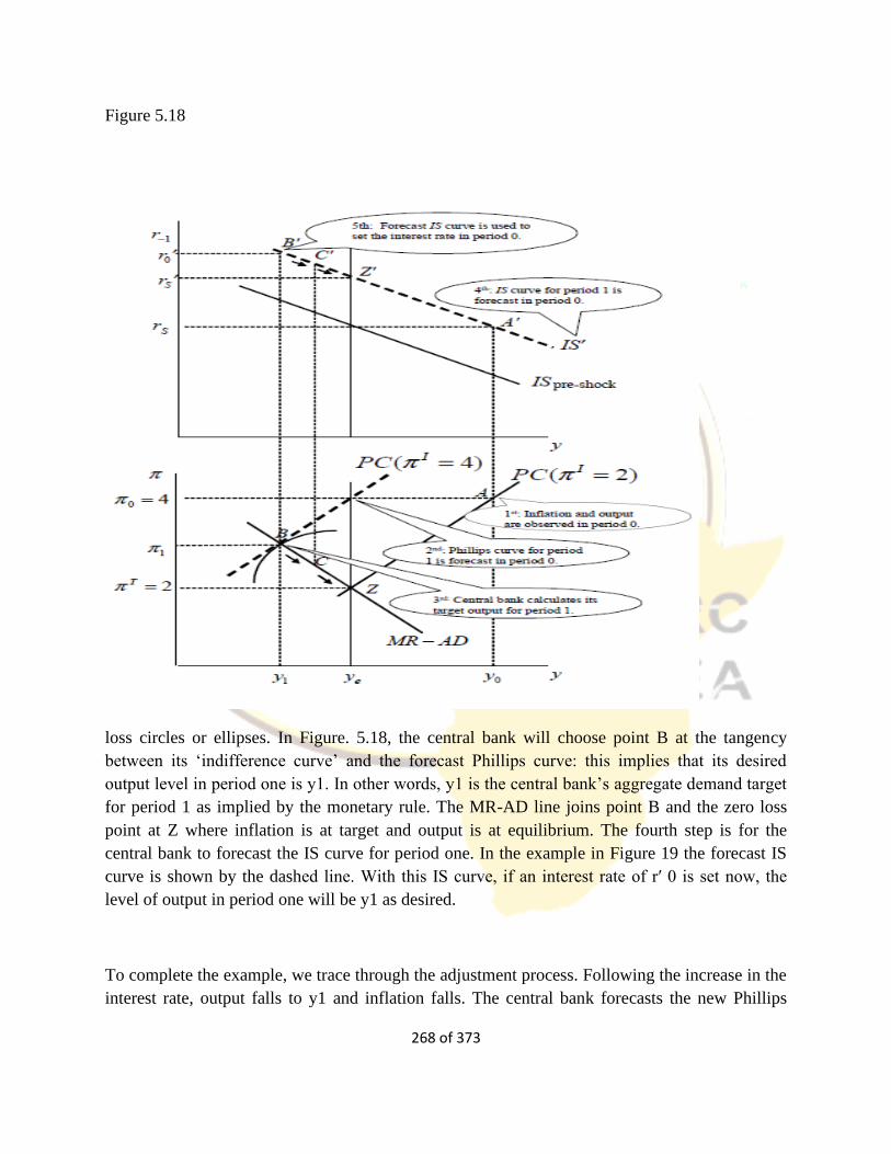
268 of 373

Figure 5.18

loss circles or ellipses. In Figure. 5.18, the central bank will choose point B at the tangency

between its ‘indifference curve’ and the forecast Phillips curve: this implies that its desired

output level in period one is y1. In other words, y1 is the central bank’s aggregate demand target

for period 1 as implied by the monetary rule. The MR-AD line joins point B and the zero loss

point at Z where inflation is at target and output is at equilibrium. The fourth step is for the

central bank to forecast the IS curve for period one. In the example in Figure 19 the forecast IS

curve is shown by the dashed line. With this IS curve, if an interest rate of r′ 0 is set now, the

level of output in period one will be y1 as desired.

To complete the example, we trace through the adjustment process. Following the increase in the

interest rate, output falls to y1 and inflation falls. The central bank forecasts the new Phillips

269 of 373

curve, which goes through point C in the Phillips diagram and it will follow the same steps to

adjust the interest rate downwards so as to guide the economy along the IS curve from C′ to Z′.

Eventually, the objective of inflation at πT = 2% is achieved and the economy is at equilibrium

unemployment,

where it will remain until a new shock or policy change arises. The MR-AD line shows the

optimal inflation-output choices of the central bank, given the Phillips curve constraint that it

faces.

An important pedagogical question is the name to give the monetary rule equation when we

show it in the πy–diagram. What it tells the central bank at t = 0 is the output level that it needs

to achieve in t = 1 if it is to minimize the loss function, given the forecast Phillips curve. Since

we are explaining the model from the central bank’s viewpoint at t = 0, what we want to convey

is that the downward sloping line in the πy–diagram shows the aggregate demand target at t = 1

implied by the monetary rule. We therefore use the label MR-AD9.

The MR-AD curve is shown in the Phillips rather than in the IS diagram because the essence of

the monetary rule is to identify the central bank’s best policy response to any shock. Both the

central bank’s preferences shown graphically by the indifference curve (part of the loss circle or

ellipse) and the trade-off it faces between output and inflation appear in the Phillips diagram.

Once the central bank has calculated its desired output response by using the forecast Phillips

curve, it is straightforward to go to the IS diagram and discover what interest rate must be set in

order to achieve this level of aggregate demand.

Using the Graphical Model

We now look briefly at different shocks so as to illustrate the role the following six

elements play in their transmission and hence in the deliberations of policy-makers

in the central bank:

9 It would be misleading to label it AD thus implying that it is the actual AD curve in π1y1– space because

the actual AD curve will include any aggregate demand shock in t = 1. If aggregate demand shocks in t =

1 are included, the curve ceases to be the curve on which the central bank bases its monetary policy in t =

0. On the other hand if an aggregate demand shock in t = 1 is excluded — so that the central bank can

base monetary policy on the curve — then it is misleading to call it the AD schedule; students would not

unreasonably be surprised if an AD schedule did not shift in response to an AD shock.

270 of 373

the inflation target, πT

the central bank’s preferences, β

the slope of the Phillips curve, α

the interest sensitivity of aggregate demand, a

the equilibrium level of output, ye

the stabilizing interest rate, rS.

A temporary aggregate demand shock is a one-period shift in the IS curve, whereas a permanent

aggregate demand shock shifts the IS curve and hence rS, the stabilizing interest rate,

permanently. An inflation shock is a temporary (oneperiod) shift in the short-run Phillips curve.

This is sometimes referred to as a temporary aggregate supply shock. An aggregate supply shock

refers to a permanent shift in the equilibrium level of output, ye. This shifts the vertical Phillips

curve.

IS shock: temporary or permanent?

In Figure 5.18, we analyzed an IS shock — but was it a temporary or a permanent one? In order

for the Central Bank to make its forecast of the IS curve, it has to decide whether the shock that

initially caused output to rise to y0 is temporary or permanent. The terms ‘temporary’ and

‘permanent’ should be interpreted from the perspective of the central bank’s decision-making

horizon. In our example, the central bank took the view that the shock would persist for another

period, so it was necessary to raise the interest rate to r′0 above the new stabilizing interest rate,

r′S.

Had the central bank forecast that the IS would revert to the pre-shock IS, then it would have

initially raised the interest rate by less since the stabilizing interest rate would have remained

equal to rS, i.e. its chosen interest rate would have been on the IS pre-shock curve in Figure 19

rather than on the IS′ curve. This highlights one of the major forecasting problems faced by the

central bank.

271 of 373

Supply shock

One of the key tasks of a basic macroeconomic model is to help illuminate how the main

variables are correlated following different kinds of shocks. We can appraise the usefulness of

the IS-PC-MR model in this respect by looking at a positive aggregate supply shock and

comparing the optimal response of the central bank and hence the output and inflation

correlations with those associated with an aggregate demand shock. A supply shock results in a

change in equilibrium output and therefore a shift in the vertical Phillips curve. It can arise from

changes that affect wage- or price-setting behaviour such as a structural change in wage-setting

arrangements, a change in taxation or in unemployment benefits or in the strength of product

market competition, which alters the mark-up.

Figure 5.19 shows the analysis of a positive supply-side shock, which raises equilibrium

output from ye to y′e. The vertical Phillips curve shifts to the right as does the short-run Phillips

curve corresponding to inflation equal to the target (shown by the PC(πI = 2, y′e)). The first

consequence of the supply shock is a fall in inflation (from 2% to zero) as the economy goes

from A to B. To decide how monetary policy should respond to this, the central bank forecasts

the Phillips curve constraint (PC (πI = 0, y′e)) for next period and chooses its optimal level of

output as shown by point C. To raise output to this level, it is necessary to cut the interest rate in

period zero to r′ as shown in the IS diagram. (Note that the stabilizing interest rate has fallen to

r′S.) The economy is then guided along the MR-AD′ curve to the new equilibrium at Z. The

positive supply shock is associated initially with a fall in inflation and a rise in output — in

contrast to the initial rise in both output and inflation in response to the aggregate demand shock.

Lags and the Taylor Rule

An optimal Taylor Rule is a policy rule that tells the central bank how to set the current interest

rate in response to shocks that result in deviations of inflation from target or output from

equilibrium or both in order to achieve its objectives. In other words, (r0 − rS) responds to (π0 −

πT) and (y0 − ye), for example:

r0 − rS = 0.5* (π0 − πT ) + 0.5*(y0 − ye). (Taylor rule)

Figure 5.19: Inflation shock: the effect of (a) greater inflation aversion of the central

bank and (b) a steeper Phillips curve

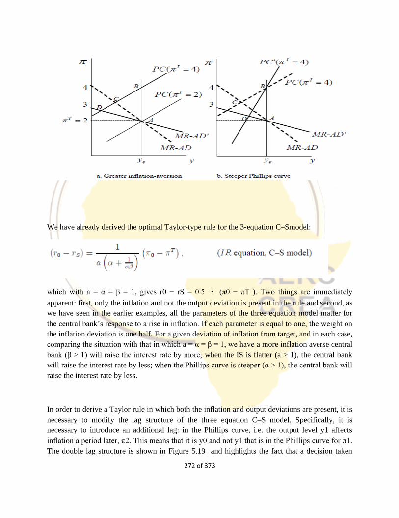
272 of 373

We have already derived the optimal Taylor-type rule for the 3-equation C–Smodel:

which with a = α = β = 1, gives r0 − rS = 0.5 ・ (π0 − πT ). Two things are immediately

apparent: first, only the inflation and not the output deviation is present in the rule and second, as

we have seen in the earlier examples, all the parameters of the three equation model matter for

the central bank’s response to a rise in inflation. If each parameter is equal to one, the weight on

the inflation deviation is one half. For a given deviation of inflation from target, and in each case,

comparing the situation with that in which a = α = β = 1, we have a more inflation averse central

bank (β > 1) will raise the interest rate by more; when the IS is flatter (a > 1), the central bank

will raise the interest rate by less; when the Phillips curve is steeper (α > 1), the central bank will

raise the interest rate by less.

In order to derive a Taylor rule in which both the inflation and output deviations are present, it is

necessary to modify the lag structure of the three equation C–S model. Specifically, it is

necessary to introduce an additional lag: in the Phillips curve, i.e. the output level y1 affects

inflation a period later, π2. This means that it is y0 and not y1 that is in the Phillips curve for π1.

The double lag structure is shown in Figure 5.19 and highlights the fact that a decision taken

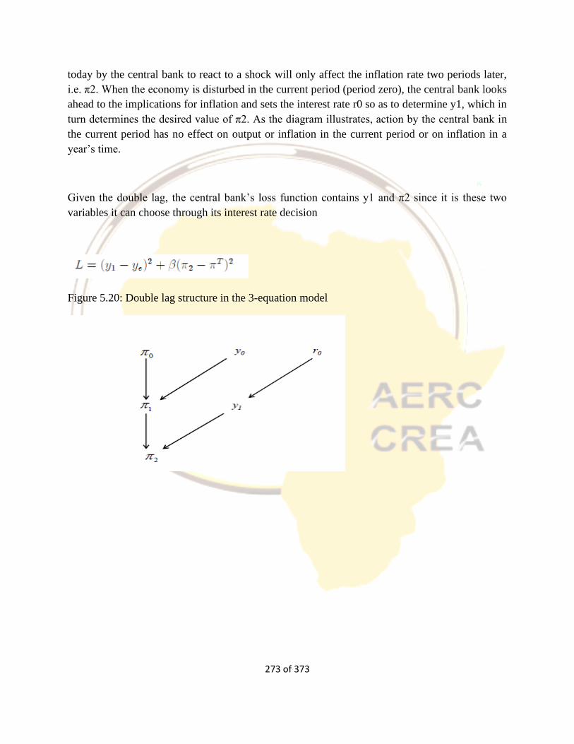
273 of 373

today by the central bank to react to a shock will only affect the inflation rate two periods later,

i.e. π2. When the economy is disturbed in the current period (period zero), the central bank looks

ahead to the implications for inflation and sets the interest rate r0 so as to determine y1, which in

turn determines the desired value of π2. As the diagram illustrates, action by the central bank in

the current period has no effect on output or inflation in the current period or on inflation in a

year’s time.

Given the double lag, the central bank’s loss function contains y1 and π2 since it is these two

variables it can choose through its interest rate decision

Figure 5.20: Double lag structure in the 3-equation model

274 of 373

Implicitly the Taylor Rule incorporates changes in the interest rate that are required as a result of

a change in the stabilizing interest rate (in the case of a permanent shift in the IS or of a supply-

side shift): rS in the rule should therefore be interpreted as the post-shock stabilizing interest rate.

It is often said that the relative weights on output and inflation in a Taylor Rule reflect the central

bank’s preferences for reducing inflation as compared to output deviations. However, we have

already seen in the single lag version of the model that although the central bank cares about

both inflation and output deviations, only the inflation deviation appears in the interest rate rule.

Although both the output and inflation deviations are present in the IR equation for the double

lag model, the relative weights on inflation and output depend only on α, the slope of the Phillips

curve. The relative weights are used only to forecast next period’s inflation.

The central bank preferences determine the interest rate response to next period’s inflation (as

embodied in the slope of the MR curve). Another way to express this result is to say that the

output term only appears in the IR equation because of the lag from a change in output to a

change in inflation.

The central bank’s loss function: graphical representation

The geometry of the central bank’s loss function can be shown in the Phillips curve

diagram. The loss function

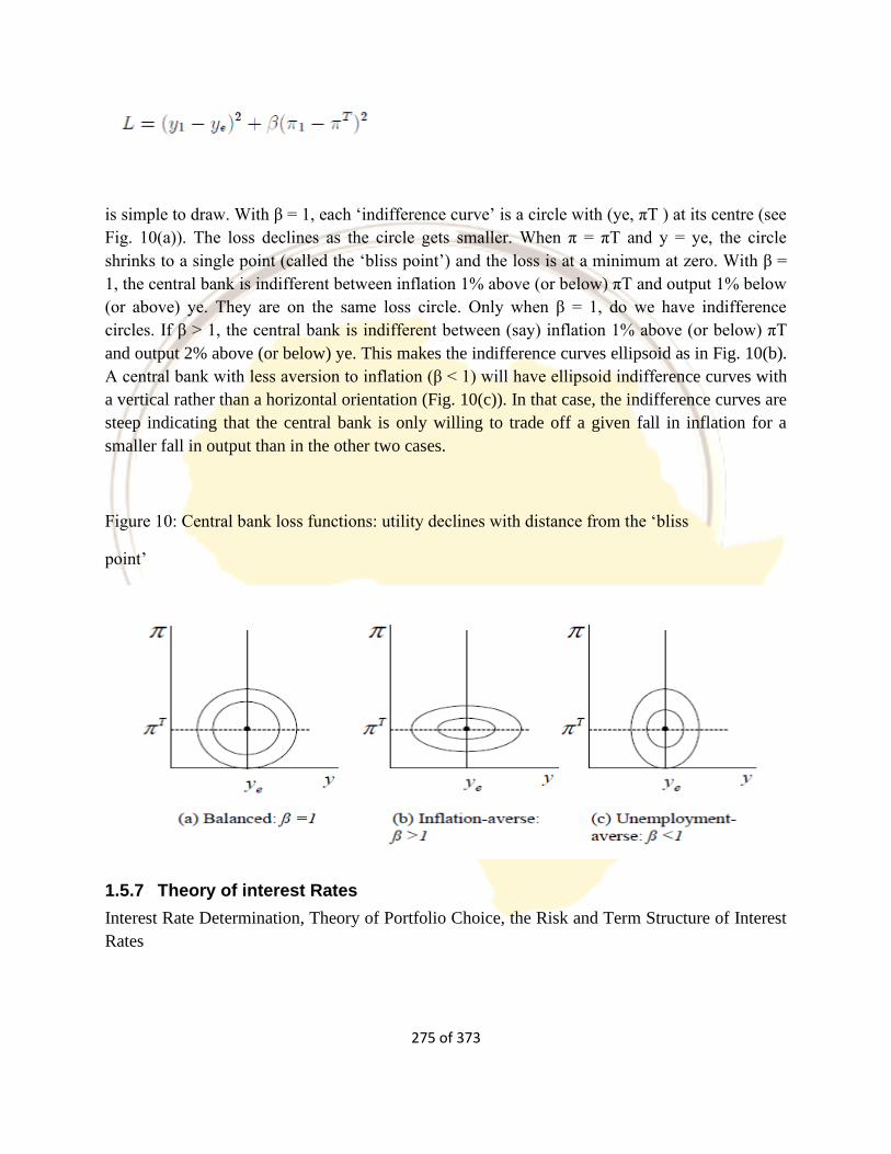
275 of 373

is simple to draw. With β = 1, each ‘indifference curve’ is a circle with (ye, πT ) at its centre (see

Fig. 10(a)). The loss declines as the circle gets smaller. When π = πT and y = ye, the circle

shrinks to a single point (called the ‘bliss point’) and the loss is at a minimum at zero. With β =

1, the central bank is indifferent between inflation 1% above (or below) πT and output 1% below

(or above) ye. They are on the same loss circle. Only when β = 1, do we have indifference

circles. If β > 1, the central bank is indifferent between (say) inflation 1% above (or below) πT

and output 2% above (or below) ye. This makes the indifference curves ellipsoid as in Fig. 10(b).

A central bank with less aversion to inflation (β < 1) will have ellipsoid indifference curves with

a vertical rather than a horizontal orientation (Fig. 10(c)). In that case, the indifference curves are

steep indicating that the central bank is only willing to trade off a given fall in inflation for a

smaller fall in output than in the other two cases.

Figure 10: Central bank loss functions: utility declines with distance from the ‘bliss

point’

1.5.7 Theory of interest Rates

Interest Rate Determination, Theory of Portfolio Choice, the Risk and Term Structure of Interest

Rates

276 of 373

The interest rate may be defined as the compensation that a borrower of capital pays to a lender

of capital for its use (Kellison, 2009)10. Thus, interest can be viewed as a form of rent that the

borrower pays to the lender to compensate for the loss of use of the capital by the lender while it

is loaned to the borrower. More practically, the interest rate is the percentage of principal

charged by the lender for the use of its money. The principal is the amount of money loaned.

Since banks borrow money from you (in the form of deposits), they also pay you an interest rate

on your money.

In other words, the interest rate is the return on bonds (all non-monetary financial assets), but we

have not so far specified explicitly the demand and supply, or the excess demand, functions for

bonds. There are two ways of doing so. One is to derive the excess demand for bonds. Bonds in

this section comprise a single homogeneous, non-monetary financial asset. Further, to get around

issues raised by maturing bonds and to establish a simple relationship between the nominal bond

price pb and the nominal interest rate R, the (homogeneous) bond is assumed to be a consol

(perpetuity), which promises a constant coupon payment of $1 in perpetuity. For this consol, pb

=1/R.

We shall also study the comparative static and dynamic determination of the macroeconomic

interest rate in the closed economy. In terms of the heritage of ideas, the theories that deal

specifically with the determination of this interest rate are the traditional classical loanable funds

theory and the Keynesian liquidity preference theory. The loanable funds theory asserts that the

bond market determines the interest rate, whereas the liquidity preference theory asserts that the

money market does so.

Nominal and real rates of interest

The Fisher equation on the interest rate

As explained in the earlier section, the Fisher equation is:

(1+re) = (1+R)/(1+πe) (1)

10 Kellison G. Stephen (2009), “The Theory of Interest”, 2nd Edition, McGraw-Hill

277 of 373

where R is the nominal interest rate, r is the real interest rate, re is the expected real interest rate

and πe is the expected inflation rate. If there exist both real bonds (i.e. promising a real rate of

return r per period) and nominal bonds (i.e. promising a nominal rate of return R per period), the

relationship between them in perfect markets would be:

(1+R) = (1+r)(1+πe) (1’)

At low values of re and πe, reπe→0, so that the Fisher equation is often simplified to:

re = R−πe

The demand and supply of bonds and interest rate determination

Since R is the nominal return on bonds, its equilibrium value is determined by:

bd(R, . . .) = bs(R, . . .) (1)

where b is the number of (homogeneous) bonds/consols. We have assumed that the demand

and supply of bonds depend on the nominal interest rate, among other variables. Both the

demand for and supply of bonds have a flow and a stock dimension.

Flows versus stocks

In terms of flows over a specified period of time, the demand for bonds corresponds to the

amount of (loanable) funds flowing or coming onto the market for lending at the various rates of

interest. Similarly, the supply of bonds corresponds to the demand for (loanable) funds from

those wanting to borrow funds during the period. However, the flow of funds that becomes

available for loans over the current period is only a small fraction of the total amount of credit

outstanding in the economy. This total amount is like a reservoir and is the stock of loanable

278 of 373

funds. The stock of loanable funds supplied at any point in time consists of all outstanding loans

plus the net additional flow supply of loanable funds, specified for each rate of interest. In stock

terms, the demand for credit is similarly the total amount already borrowed plus the net

additional amounts that the borrowers wish to borrow at each rate of interest. In modern

economies, a major part of this demand often comes from the existing public debt.

In markets with long-term contracts, some of the borrowers and lenders are already committed to

loans made at rates prevailing in the past. In such a case, the proper market for determining the

current rate of interest is that in terms of flows: the flow market is the actual operating market for

bonds in any given period, with borrowers (sellers of bonds) entering it to borrow and lenders

(buyers of bonds) entering it to lend funds. However, note that the pre-existing stock of bonds

does exert a strong background influence on the flow demands and supplies since parts of this

stock of bonds will be expected by borrowers and lenders to mature sooner or later and, over

time, become flows available for renegotiation.

The flow supply of funds can be interpreted as that part of the stock that has come up for

renegotiation plus the additions being made currently. The net new supply of funds to the credit

market in any period t comes from two sources:

(i) Current (private) saving in the economy.

(ii) Excess supply of money made available for loans, with the excess supply resulting from

changes in the public’s desired balances or in the supply of money.

The supply of money depends on the monetary base and the inside money created by financial

intermediaries. The overall supply of funds in period t is the net new supply from the above two

sources plus:

(iii) Funds becoming available from loans that have matured in period t.

The flow demand for loans is from net new borrowers and those who wish to renew existing

279 of 373

loans.

The net new demand for loans comes from:

Current investment in the economy.

Bond-financed government deficits.

The flow demand for loans in period t is from (iv) and (v), plus:

Demand for credit from those whose loans have matured.

Assuming (iii) and (vi) to be equal, the loanable funds theory in flow terms specifies the real

demand (f d) and supply (f s) functions of loanable funds as:

f s = s(r, . . .)+(θ.M0s/P−md(R, . . .)) (2)

f d = i(r, . . .)+(g −t) (3)

where:

f s = real flow supply of loanable funds (demand for bonds)

f d = real flow demand for loanable funds (supply of bonds)

s = real saving

i = real investment

g = real government expenditures

t = real government revenues

M0s = supply of the nominal monetary base

θ = monetary base to money supply multiplier (= ∂Ms/∂M0)

md = demand for real balances

280 of 373

P = price level.

We have assumed that the government deficit (g−t) is wholly bond-financed and that r and R are

related by the Fisher equation. In partial equilibrium analysis, the equilibrium value of the

market rate of interest is determined by:

s(r, . . .)+(θ.M0s/P−md(R, . . .)) = i(r, . . .)+(g −t) (3)

Note that the left side of (3) represents the demand for bonds and the right side represents the

supply of bonds. (3) is the statement that the interest rate is determined by the equilibrium in the

flow part of the bond market.

Long-run determination of the interest rate

Equation (3) specifies the determination of the short-run interest rate and shows that, although

the interest rate is determined by the excess demand for loanable funds, it is not independent of

the excess demand for money:8 excess money demand raises the interest rate and excess money

supply lowers it. However, money supply and demand enter the determination of the interest rate

only if there is disequilibrium in the money market.

In the long run (general equilibrium) the money market would be in equilibrium, so that the

excess money demand term on the left side of (3) is zero. Hence, the long-run version

of the bond market analysis becomes:

s(r, . . .) = i(r, . . .)+(g −t) (4)

or:

sn(r, . . .) = i(r, . . .)

281 of 373

where sn is national saving (= s+(t−g)). In the context of the closed economy, (4) is also

the statement of equilibrium in the commodity sector of the economy.

Classical heritage: the loanable funds theory of the rate of interest

The traditional classical economists (prior to Keynes) had generally favored the specification of

the overall equilibrium in terms of the bond, money and labor markets, with the labor market

determining employment and, through the production function, output; the bond market

determining the interest rate, and the market for money determining the price level.

Its theory of the determination of the interest rate (or its inverse, the price of bonds for bonds

specified as consols which have fixed coupon payments payable perpetually) was known as the

loanable funds theory. It asserted that the interest rate was determined in the bond market by

equilibrium between the demand and supply of “loanable funds,” which was its synonym for the

current term “bonds.” Given the discussion so far in this chapter, we can distinguish the

following three aspects of the loanable funds theory:

Partial equilibrium (short-run) determination of the interest rate.

General equilibrium (long-run) determination of the interest rate.

Dynamic movement of the interest rate.

The traditional classical economists did not have a distinction (until the advent of Fisher’s

equation) between the real and nominal interest rate, so that they normally referred to the market

interest rate R as the determinant of investment and saving. Following their pattern of analysis,

we will specify the investment function in the following as i(R), rather than our usual i(r). They

also did not have a government sector with outstanding bond-financed budget deficits. Further,

the role of financial intermediaries and the monetary base in the money creation process were not

fully understood.

Given these simplifications, the demand and supply functions of the loanable funds

282 of 373

theory were:

Pf s = Ps(R, y)+[Ms −Md]

Pf d = Pi(R)

Therefore, the short-run (i.e. partial equilibrium) determination of the interest rate according

to the loanable funds theory was specified by:

s(R, y)+(1/P)[Ms −Md] = i(R) (5)

so that:

R = ϕ(P, y; (M −Md)) (6)

which allows both the commodity market and the money market shifts to change the interest

rate.

The long-run version of the loanable funds theory assumed general equilibrium in the

economy. Therefore, for this version, M − Md = 0, so that the long-run loanable funds

theory became:

i(R) = s(R, y)

Further, long-run equilibrium in the commodity and labor markets ensures that output will be at

the full-employment level (yf ), so that (7) becomes:

283 of 373

i(R) = s(R, yf ) (8)

That is, the long-run interest rate is determined by the equality of investment and saving at full-

employment output, so that its main determinants are the propensity to save, the production

capacity of the economy, and investment. In particular, this interest rate is not altered by shifts in

the demand or supply of money.

For the dynamic movement of the interest rate when there is disequilibrium in the economy, the

loanable funds theory asserted that the interest rate is determined by the excess demand or supply

of loanable funds: it falls (while the bond price rises) if there is an excess demand for loanable

funds, and rises (while the bond price falls) if there is an excess supply of loanable funds.

Therefore, this theory’s assertion for dynamic adjustments in the interest rate is:

R = f (Ebd) ∂R/∂( Ebd) < 0 (9)

Note that, since changes in the money supply and demand alter the excess demand for bonds,

they will also affect the dynamic path of the interest rate.

To conclude on the relevance of the excess money supply in changing the nominal interest rate,

only the long-run version of the loanable funds theory asserted its irrelevance for the

determination of the interest rate. However, this long-run version, which is the statement that the

interest rate is determined by saving at full employment and investment, is the one usually

remembered as the statement of the loanable funds theory. Adapting the loanable funds theory to

the modern economy requires the introduction of the government sector, the central bank and the

financial sector into the component functions of this theory.

Loanable funds theory in the modern classical approach

In recent years, the modern version of the classical paradigm has reasserted continuous market

clearance for the labor markets, as for the other markets, and with its assumption of rational

expectations has further asserted the possibility of disequilibrium (due to expectational errors) in

any market as at best a very transitory state. That is, with the labor and money markets clearing

284 of 373

continuously, there would exist full employment in the economy and the excess demand in the

money market would be zero. Consequently, for the modern classical school, the theory of

interest reverts to the long-run version of the traditional loanable funds theory, with the

difference that it is now intended to be not only the long-run theory but also the short-run theory

of the rate of interest as far as systematic or anticipated changes in the money supply are

concerned.14 However, such a short-run theory could still diverge from its long-run version

because of random influences

operating on the economy in the short run. These cannot be anticipated under rational

expectations and would cause a divergence of the short-run interest rate from its long-run level.

The modern classical version of the loanable funds theory, therefore, extends and differs from

the traditional classical one in various ways. Among the differences are:

The role of financial intermediaries, as discussed earlier.

The addition of Fisher’s equation connecting the real and nominal interest rates in perfect capital

markets.

The distinction in the modern version between the anticipated and unanticipated values of the

relevant variables, among which are the money supply, the other determinants of aggregate

demand and the rate of inflation. Anticipated money supply increases cause anticipated inflation

without changing the real interest rate and, therefore, increase the nominal rate by the anticipated

rate of inflation, as specified by the Fisher equation. Unanticipated money supply growth lowers

the real rate and will lower the market rate of interest.

Ricardian equivalence, which makes national saving independent of the (anticipated) fiscal

deficit and therefore removes such deficits from the determinants of the demand and supply of

loanable funds. In this case, anticipated deficits would not affect the interest rate.

In the short run, the traditional classical economists allowed deviations from full employment

under the impact of money supply changes and the impact of these changes on saving. The

modern classical economists allow such a deviation for only unanticipated money supply

changes.

Therefore, the short-run deviations of output from its full employment level under the impact of

anticipated money supply changes could, in the short run, affect the interest rate under the

traditional version of the loanable funds theory but not under its modern version.

285 of 373

Note that outside the confines of long-run general equilibrium analysis, the interest rate is not

merely the reward for postponing consumption, it is also the return on lending, which is the act

of parting with liquidity, i.e. not holding money. The latter was a major contention of Keynes

and is a fundamental part of Keynesian beliefs.

Keynesian heritage: the liquidity preference theory of the interest rate

Keynes’s General Theory (1936) challenged the loanable funds theory on the grounds that the

interest rate was not the reward for saving but was rather an inducement to part with liquidity. He

summarized his views in the statement:

[Once the individual has made his decision on consumption versus saving out of his income],

there is a further decision which awaits him, namely, in what form he will hold the command

over future consumption which he has reserved, whether out of his current income or from

previous savings. Does he want to hold it in the form of immediate, liquid command (i.e. in

money or its equivalent)? Or is he prepared to part with immediate command for a specified or

indefinite period.…

It should be obvious that the rate of interest cannot be a return to saving or waiting as such. For if

a man hoards his savings in cash, he earns no interest, though he saves just as much as before.

On the contrary,…, the rate of interest is the reward for parting with liquidity for a specified

period.… Thus the rate of interest at any time, being the reward for parting with liquidity, is a

measure of the unwillingness of those who possess money to part with their liquid control over

it. The rate of interest is not the “price” which brings into equilibrium the demand for resources

to invest with the readiness to abstain from present consumption.

It is the “price” which equilibrates the desire to hold wealth in the form of cash with the available

quantity of cash.…If this explanation is correct, the quantity of money is the other factor, which,

in conjunction with liquidity preference, determines the actual rate

of interest in given circumstances.(Keynes, 1936, pp. 166–8).

286 of 373

First, consider Keynes’s argument in terms of its general notion that the interest rate is the

reward for parting with liquidity. This is definitely true in a world with uncertainty. Savers have

a choice as to the form in which to hold their savings. They may hold these in a monetary form

or lend it. If the level of the interest rate determines their division of savings into money balances

versus loans, the interest rate can be called the reward for parting with liquidity in the process of

lending. However, if the interest rate also influences the level of savings, then it may also be

called a reward for postponing consumption. Both cases apply in the real

world.

Now consider Keynes’s argument formally in terms of the equilibrium relationship of the

monetary sector. Keynes’s money market equilibrium relationship for an exogenously given

money supply

M is:

M = kPy+L(R) (10)

Equation (10) determines R if it is assumed that P and y are exogenously given. This is not true

of the Keynesian model and is not true for Keynes’s own ideas in general. In his theory, output,

interest and prices were determined simultaneously so that R is not determined merely by (10): it

is also influenced by the saving and investment decisions of the expenditure sector as well as by

the labor market structure. Hence, the interest rate is not merely the reward for parting with

liquidity, even though that may seem to be the most proximate or closely related cause.

Dynamics of the liquidity preference theory

According to Keynes’s liquidity preference theory, the dynamic movements of the interest rate

are determined by the excess demand for money. Hence, it was asserted that:

R = f (Emd) ∂R/∂(Emd) > 0

(11)

287 of 373

so that:

∂R/∂(Md −Ms) > 0 (12)

The argument behind this assertion runs as follows. According to Keynes an excess demand for

money by individuals would make them sell bonds in order to obtain the extra money balances

they want. These bond sales will lower bond prices, which will raise the interest rate.

Theory of Portfolio Choice

All the determining factors we have just discussed can be assembled into the theory of portfolio

choice, which tells us how much of an asset people will want to hold in their portfolios. It states

that, holding all other factors constant:

The quantity demanded of an asset is positively related to wealth.

The quantity demanded of an asset is positively related to its expected return relative to

alternative assets.

The quantity demanded of an asset is negatively related to the risk of its returns relative to

alternative assets.

The quantity demanded of an asset is positively related to its liquidity relative to

alternative assets.

Supply and Demand in the Bond Market:

Our first approach to the analysis of interest-rate determination looks at supply and demand in

the bond market so that we can better understand how the prices of bonds are determined.

Thanks to our knowledge earlier of how interest rates are measured, we know that each bond

price is associated with a particular level of the interest rate. Specifically, the negative

relationship between bond prices and interest rates means that when a bond’s price rises, its

interest rate falls, and vice versa.

288 of 373

The first step in our analysis is to obtain a bond demand curve, which shows the relationship

between the quantity demanded and the price when all other economic variables are held

constant (that is, values of other variables are taken as given). You may recall from previous

economics courses that the assumption that all other economic variables are held constant is

called ceteris paribus, which means “other things being equal” in Latin.

Demand Curve:

To clarify and simplify our analysis, let’s consider the demand for one-year discount bonds,

which make no coupon payments but pay the owner the $1,000 face value in a year. If the

holding period is one year, then, as we saw in Chapter 4, the return on the bonds is known

absolutely and is equal to the interest rate as measured by the yield to maturity. This means that

the expected return on this bond is equal to the interest rate i, which, using Equation 6 in Chapter

4, is

i = Re =(F – P)/P

where i = interest rate = yield to maturity

Re = expected return

F = face value of the discount bond

P = initial purchase price of the discount bond

This formula shows that a particular value of the interest rate corresponds to each bond price. If

the bond sells for $950, the interest rate and expected return are

($1,000 - $950)/$950 = 0.053 = 5.3%

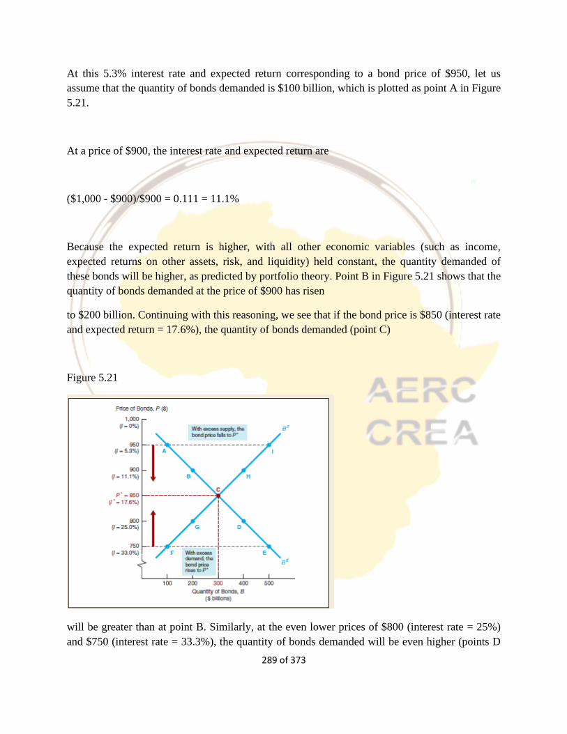
289 of 373

At this 5.3% interest rate and expected return corresponding to a bond price of $950, let us

assume that the quantity of bonds demanded is $100 billion, which is plotted as point A in Figure

5.21.

At a price of $900, the interest rate and expected return are

($1,000 - $900)/$900 = 0.111 = 11.1%

Because the expected return is higher, with all other economic variables (such as income,

expected returns on other assets, risk, and liquidity) held constant, the quantity demanded of

these bonds will be higher, as predicted by portfolio theory. Point B in Figure 5.21 shows that the

quantity of bonds demanded at the price of $900 has risen

to $200 billion. Continuing with this reasoning, we see that if the bond price is $850 (interest rate

and expected return = 17.6%), the quantity of bonds demanded (point C)

Figure 5.21

will be greater than at point B. Similarly, at the even lower prices of $800 (interest rate = 25%)

and $750 (interest rate = 33.3%), the quantity of bonds demanded will be even higher (points D

290 of 373

and E). The curve Bd, which connects these points, is the demand curve for bonds. It has the

usual downward slope, indicating that at lower prices of the bond (everything else being equal),

the quantity demanded is higher.

Supply Curve:

An important assumption behind the demand curve for bonds in Figure 5.21 is that all other

economic variables besides the bond’s price and interest rate are held constant. We use the same

assumption in deriving a supply curve, which shows the relationship between the quantity

supplied and the price when all other economic variables are held constant.

In Figure 5.21, when the price of the bonds is $750 (interest rate = 33.3%), point F shows that

the quantity of bonds supplied is $100 billion for the example we are considering. If the price is

$800, the interest rate is the lower rate of 25%. Because at this Although our analysis indicates

that the demand curve is downward-sloping, it does not imply that the curve is a straight line. For

ease of exposition, however, we will draw demand curves and supply curves as straight lines.

interest rate it is now less costly to borrow by issuing bonds, firms will be willing to borrow

more through bond issues, and the quantity of bonds supplied is at the higher level of $200

billion (point G). An even higher price of $850, corresponding to a lower rate of 17.6%, results

in a larger quantity of bonds supplied of $300 billion (point C). Higher prices of $900 and $950

result in even lower interest rates and even greater quantities of bonds supplied (points H and I).

The Bs curve, which connects these points, is the supply curve for bonds. It has the usual upward

slope found in supply curves, indicating that as the price increases (everything else being equal),

the quantity supplied increases.

Market Equilibrium:

In economics, market equilibrium occurs when the amount that people are willing to buy

(demand) equals the amount that people are willing to sell (supply) at a given price. In the bond

market, this is achieved when the quantity of bonds demanded equals the quantity of bonds

supplied:

Bd = Bs (1)

291 of 373

In Figure 5.21, equilibrium occurs at point C, where the demand and supply curves intersect at a

bond price of $850 (interest rate of 17.6%) and a quantity of bonds of $300 billion. The price of

P* = 850, where the quantity demanded equals the quantity supplied, is called the equilibrium or

market-clearing price. Similarly, the interest rate of i* = 17.6% that corresponds to this price is

called the equilibrium or market-clearing interest rate.

The concepts of market equilibrium and equilibrium price or interest rate are useful because the

market tends to head toward them. We can see this in Figure 5.21 by first looking at what

happens when we have a bond price that is above the equilibrium price. When the price of bonds

is set too high, at, say, $950, the quantity of bonds supplied at point I is greater than the quantity

of bonds demanded at point A. A situation like this, in which the quantity of bonds supplied

exceeds the quantity of bonds demanded, is called a condition of excess supply. Because people

want to sell more bonds than others want to buy, the price of the bonds will fall, as shown by the

downward arrow in the figure at the bond price of $950. As long as the bond price remains above

the equilibrium price, an excess supply of bonds will continue to be available, and the price of

bonds will continue to fall. This decline will stop only when the price has reached the

equilibrium price of $850, the price at which the excess supply of bonds has been eliminated.

Now let’s look at what happens when the price of bonds is below the equilibrium price. If the

price of the bonds is set too low, at, say, $750, the quantity demanded at point E is greater than

the quantity supplied at point F. This is called a condition of excess demand. People now want to

buy more bonds than others are willing to sell, so the price of bonds will be driven up, as

illustrated by the upward arrow in the figure at the bond price of $750. Only when the excess

demand for bonds is eliminated by the bond price rising to the equilibrium level of $850 is there

no further tendency for the price to rise.

We can see that the concept of equilibrium price is a useful one because it indicates where the

market will settle. Because each price on the vertical axis of Figure 5.21 corresponds to a

particular value of the interest rate, the same diagram also shows that the interest rate will head

toward the equilibrium interest rate of 17.6%. When the of the bond is above the equilibrium

price, and an excess supply of bonds results. The price of the bond then falls, leading to a rise in

the interest rate toward the equilibrium level. Similarly, when the interest rate is above the

equilibrium level, as it is when it is at 33.3%, an excess demand for bonds occurs, and the bond

price rises, driving the

interest rate back down to the equilibrium level of 17.6%.

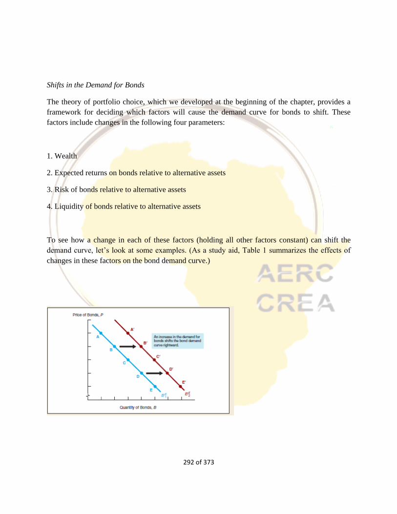
292 of 373

Shifts in the Demand for Bonds

The theory of portfolio choice, which we developed at the beginning of the chapter, provides a

framework for deciding which factors will cause the demand curve for bonds to shift. These

factors include changes in the following four parameters:

1. Wealth

2. Expected returns on bonds relative to alternative assets

3. Risk of bonds relative to alternative assets

4. Liquidity of bonds relative to alternative assets

To see how a change in each of these factors (holding all other factors constant) can shift the

demand curve, let’s look at some examples. (As a study aid, Table 1 summarizes the effects of

changes in these factors on the bond demand curve.)

293 of 373

Wealth When the economy is growing rapidly in a business cycle expansion and wealth is

increasing, the quantity of bonds demanded at each bond price (or interest rate) increases, as

shown in Figure 5.22. To see how this works, consider point B on the initial demand curve for

bonds, Bd1. With higher wealth, the quantity of bonds demanded at the same price must rise, to

point B1. Similarly, for point D, the higher wealth causes the quantity demanded at the same

bond price to rise to point D1. Continuing with this reasoning for every point on the initial

demand curve Bd, we can see that the demand curve shifts to the right from Bd1 to Bd2, as

indicated by the arrows.

We can conclude that in a business cycle expansion with growing wealth, the demand for bonds

rises and the demand curve for bonds shifts to the right. Applying the same reasoning, in a

recession, when income and wealth are falling, the demand Another factor that affects wealth is

the public’s propensity to save. If households save more, wealth increases and, as we have seen,

the demand for bonds rises and the demand curve for bonds shifts to the right. Conversely, if

people save less, wealth and the demand for bonds fall, and the demand curve shifts to the left.

Expected Returns For a one-year discount bond and a one-year holding period, the expected

return and the interest rate are identical, so nothing other than today’s interest rate affects the

expected return. For bonds with maturities of greater than one year, the expected return may

differ from the interest rate. For example, Table 1, that a rise in the interest rate on a long-term

bond from 10% to 20% would lead to a sharp decline in price and a very large negative return.

Hence, if people began to think that interest rates would be higher next year than they had

originally anticipated, the expected return today on long-term bonds would fall, and the quantity

demanded would fall at each interest rate. Higher expected future interest rates lower the

expected return for longterm bonds, decrease the demand, and shift the demand curve to the left.

By contrast, an expectation of lower future interest rates would mean that longterm bond prices

would be expected to rise more than originally anticipated, and the resulting higher expected

return today would raise the quantity demanded at each bond price and interest rate. Lower

expected future interest rates increase the demand for long-term bonds and shift the demand

curve to the right (as in Figure 5.22). Changes in expected returns on other assets can also shift

the demand curve for bonds. If people suddenly become more optimistic about the stock market

and beginto expect higher stock prices in the future, both expected capital gains and expected

returns on stocks will rise. With the expected return on bonds held constant, the expected return

on bonds today relative to stocks will fall, lowering the demand for bonds and shifting the

294 of 373

demand curve to the left. An increase in expected return on alternative assets lowers the demand

for bonds and shifts the demand curve to the left.

A change in expected inflation is likely to alter expected returns on physical assets (also called

real assets), such as automobiles and houses, which affect the demand for bonds. An increase in

expected inflation from, say, 5% to 10% will lead to higher prices on cars and houses in the

future and hence higher nominal capital gains. The resulting rise in the expected returns today on

these real assets will lead to a fall in the expected return on bonds relative to the expected return

on real assets today and thus cause the demand for bonds to fall. Alternatively, we can think of

the rise in expected inflation as lowering the real interest rate on bonds, and thus the resulting

decline in the relative expected return on bonds will cause the demand for bonds to fall. An

increase in the expected rate of inflation lowers the expected return on bonds, causing their

demand to decline and the demand curve to shift to the left.

Risk: If prices in the bond market become more volatile, the risk associated with bonds

increases, and bonds become a less attractive asset. An increase in the riskiness of bonds causes

the demand for bonds to fall and the demand curve to shift to the left. Conversely, an increase in

the volatility of prices in another asset market, such as the stock market, would make bonds more

attractive. An increase in the riskiness of alternative assets causes the demand for bonds to rise

and the demand curve to shift to the right (as in Figure5. 22).

Liquidity If more people started trading in the bond market, and as a result it became easier to

sell bonds quickly, the increase in their liquidity would cause the quantity of bonds demanded at

each interest rate to rise. Increased liquidity of bonds results in an increased demand for bonds,

and the demand curve shifts to the right (see Figure 5.22). for bonds falls, and the demand curve

shifts to the left. shifts the demand curve to the left. The reduction of brokerage commissions for

trading common stocks that occurred when the fixed-rate commission structure was abolished in

1975, for example, increased the liquidity of stocks relative to bonds, and the resulting lower

demand for bonds shifted the demand curve to the left.

Shifts in the Supply of Bonds

Certain factors can cause the supply curve for bonds to shift. Among these factors are:

1. Expected profitability of investment opportunities

295 of 373

2. Expected inflation

3. Government budget deficits

We will look at how the supply curve shifts when each of these factors changes (all others

remaining constant). (As a study aid, Table 3 summarizes the effects of changes in these factors

on the bond supply curve.) Expected Profitability of Investment Opportunities When

opportunities for profitable plant and equipment investments are plentiful, firms are more willing

to borrow to finance these investments. When the economy is growing rapidly, as in a business

cycle expansion, investment opportunities that are expected to be profitable abound, and the

quantity of bonds supplied at any given bond price increases . Therefore, in a business cycle

expansion, the supply of bonds increases and the supply curve shifts to the right. Likewise, in a

recession, when far fewer profitable investment opportunities are expected, the supply of bonds

falls and the supply curve shifts to the left.

Expected Inflation The real cost of borrowing is most accurately measured by the real interest

rate, which equals the (nominal) interest rate minus the expected inflation rate. For a given

interest rate (and bond price), when expected inflation increases, the real cost of borrowing falls;

hence, the quantity of bonds supplied increases at any given bond price. An increase in expected

inflation

causes the supply of bonds to increase and the supply curve to shift to the right (see Figure 5.23)

and a decrease in expected inflation causes the supply of bonds to decrease and the supply curve

to shift to the left.

Government Budget Deficits The activities of the government can influence the supply of bonds

in several ways. The U.S. Treasury issues bonds to finance government deficits, caused by gaps

between the government’s expenditures and its revenues. When these deficits are large, the

Treasury sells more bonds, and the quantity of bonds supplied at each bond price increases.

Higher government deficits increase the supply of bonds and shift the supply curve to the right

(see Figure 5.23). On the other hand, government surpluses, as occurred in the late 1990s,

decrease the supply of bonds and shift the supply curve to the left.

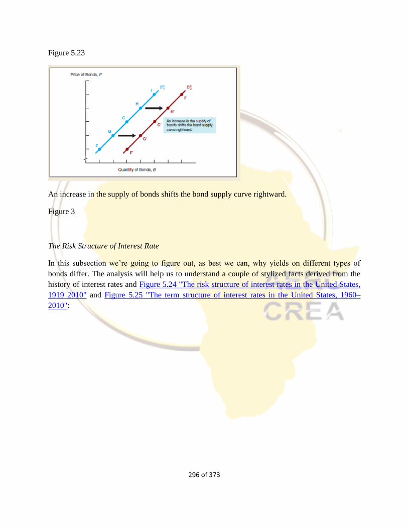
296 of 373

Figure 5.23

An increase in the supply of bonds shifts the bond supply curve rightward.

Figure 3

The Risk Structure of Interest Rate

In this subsection we’re going to figure out, as best we can, why yields on different types of

bonds differ. The analysis will help us to understand a couple of stylized facts derived from the

history of interest rates and Figure 5.24 "The risk structure of interest rates in the United States,

1919 2010" and Figure 5.25 "The term structure of interest rates in the United States, 1960–

2010":

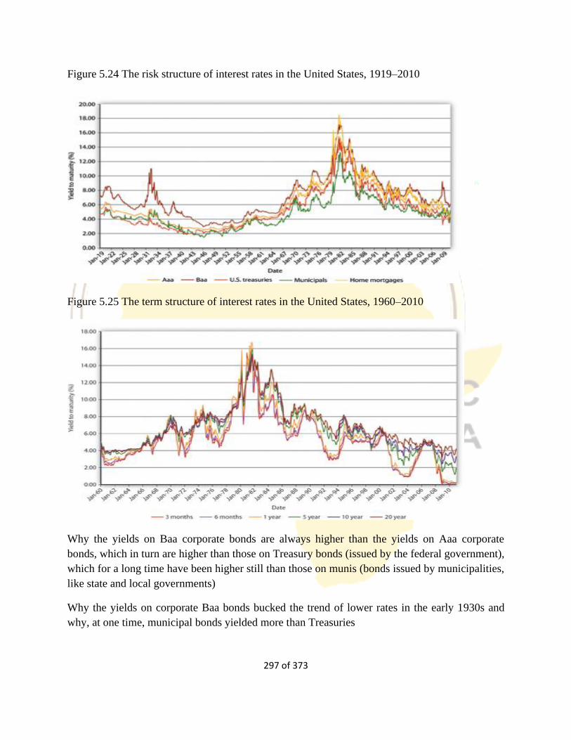
297 of 373

Figure 5.24 The risk structure of interest rates in the United States, 1919–2010

Figure 5.25 The term structure of interest rates in the United States, 1960–2010

Why the yields on Baa corporate bonds are always higher than the yields on Aaa corporate

bonds, which in turn are higher than those on Treasury bonds (issued by the federal government),

which for a long time have been higher still than those on munis (bonds issued by municipalities,

like state and local governments)

Why the yields on corporate Baa bonds bucked the trend of lower rates in the early 1930s and

why, at one time, municipal bonds yielded more than Treasuries

298 of 373

Why bonds issued by the same economic entity (the U.S. government) with different maturities

generally, but not always, have different yields and why the rank ordering changes over time

Figure 5.24 "The risk structure of interest rates in the United States, 1919–2010", which holds

maturity constant, is the easiest to understand because we’ve already discussed the major

concepts. We’ll tackle it, and what economists call the risk structure of interest rates, first.

Investors care mostly about three things: risk, return, and liquidity. Because the bonds in Figure

5.25 "The risk structure of interest rates in the United States, 1919–2010" are all long-term

bonds, their expected relative returns might appear at first glance to be identical. Investors know,

however, that bonds issued by different economic entities have very different probabilities of

defaulting. Specifically, they know the following:

Many governments like the U.S. government has never defaulted on its bonds and is extremely

unlikely to do so because even if its much-vaunted political stability were to be shattered and its

efficient tax administration (that wonderful institution, the Internal Revenue Service [IRS]) were

to stumble, it could always meet its nominal obligations by creating money. (That might create

inflation, as it has at times in the past. Nevertheless, except for a special type of bond called

TIPS, the government and other bond issuers promise to pay a nominal value, not a real

[inflation-adjusted] sum, so the government does not technically default when it pays its

obligations by printing money.)

Municipalities have defaulted on their bonds in the past and could do so again in the future

because, although they have the power to tax, they do not have the power to create money at

will. (Although in the past, most recently during the Great Depression, some issued money-

like—let’s call them extra legal—bills of credit, or chits.) Nevertheless, the risk of default on

municipal bonds (aka munis) is often quite low, especially for revenue bonds, upon which

specific taxes and fees are pledged for interest payments.

Interest earned on munis is exempt from most forms of income taxation, while interest earned on

Treasuries and corporate bonds is fully taxable.

Corporations are more likely to default on their bonds than governments are because they must

rely on business conditions and management acumen. They have no power to tax and only a

limited ability to create the less-liquid forms of money, a power that decreases in proportion to

their need! (I’m thinking of gift cards, declining balance debit cards, trade credit, and so forth.)

Some corporations are more likely to default on their bonds than others. Several credit-rating

agencies, including Moody’s and Standard and Poor’s, assess the probability of default and

assign grades to each bond. There is quite a bit of grade inflation built in (the highest grade being

not A or even A+ but Aaa), the agencies are rife with conflicts of interest, and the market usually

senses problems before the agencies do. Nevertheless, bond ratings are a standard proxy for

default risk because, as Figure 5.25 "Default rates on bonds rated by Moody’s from 1983 to

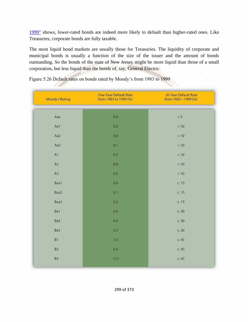
299 of 373

1999" shows, lower-rated bonds are indeed more likely to default than higher-rated ones. Like

Treasuries, corporate bonds are fully taxable.

The most liquid bond markets are usually those for Treasuries. The liquidity of corporate and

municipal bonds is usually a function of the size of the issuer and the amount of bonds

outstanding. So the bonds of the state of New Jersey might be more liquid than those of a small

corporation, but less liquid than the bonds of, say, General Electric.

Figure 5.26 Default rates on bonds rated by Moody’s from 1983 to 1999

300 of 373

Equipped with this knowledge, we can easily understand the reasons for the rank ordering in

Figure 5.23 "The risk structure of interest rates in the United States, 1919–2010".Figure 5.26

"Default rates on bonds rated by Moody’s from 1983 to 1999", by the way, should not be taken

as evidence that credit rating agencies provide investors with useful information. Before 1970 or

so, they sold ratings to investors and generally did a good job of ranking risks in a competitive

market for ratings. Thereafter, however, they formed a government-sanctioned oligopoly and

began to charge issuers for ratings. The resulting conflict of interest degraded the quality of

ratings to the point that the big three rating agencies failed to predict the crises of 1997–98 in

Southeast Asia and 2008 in the United States and Europe. Today, few investors still take their

ratings seriously, as evidenced by the fact that Treasury bond prices actually increased after U.S.

government bonds were downgraded by credit rating agency Standard and Poor’s in August

2011. Corporate Baa bonds have the highest yields because they have the highest default risk (of

those graphed), and the markets for their bonds are generally not very liquid. Corporate Aaa

bonds are next because they are relatively safer (less default risk) than Baa bonds and they may

be relatively liquid, too. U.S. Treasuries are extremely safe and the markets for them are

extremely liquid, so their yields are lower than those of corporate bonds. In other words,

investors do not need as high a yield to own Treasuries as they need to own corporates. Another

way to put this is that investors place a positive risk premium (to be more precise, a credit or

default risk, liquidity, and tax premium) on corporate bonds.

They would have higher yields and hence would be above the Baa line because they would have

a higher default risk, the same tax treatment, and perhaps less liquidity.

The low yield on munis is best explained by their tax exemptions. Before income taxes became

important, the yield on munis was higher than that of Treasuries, as we would expect given that

Treasuries are more liquid and less likely to default. During World War II, investors, especially

wealthy individuals, eager for tax-exempt income and convinced that the fiscal problems faced

by many municipalities during the depression were over, purchased large quantities of municipal

bonds, driving their prices up (and their yields down). Almost all the time since, tax

considerations, which are considerable given our highest income brackets exceed 30 percent,

have overcome the relatively high default risk and illiquidity of municipal bonds, rendering them

more valuable than Treasuries, ceteris paribus.

Risk, after-tax returns, and liquidity also help to explain changes in spreads, the difference

between yields of bonds of different types (the distance between the lines. The big spike in Baa

bond yields in the early 1930s, the darkest days of the Great Depression, was due to one simple

cause: companies with Baa bond ratings were going belly-up left and right, leaving bondholders

hanging. As Figure 5.27 shows, companies that issued Aaa bonds, municipalities, and possibly

even the federal government were also more likely to default in that desperate period, but they

were not nearly as likely to as weaker companies. Yields on their bonds therefore increased, but

only a little, so the spread between Baa corporates and other bonds increased considerably in

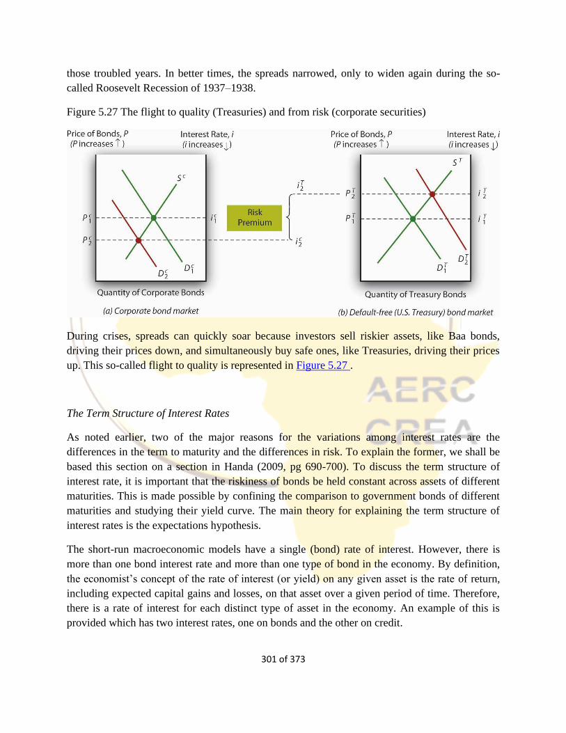
301 of 373

those troubled years. In better times, the spreads narrowed, only to widen again during the so-

called Roosevelt Recession of 1937–1938.

Figure 5.27 The flight to quality (Treasuries) and from risk (corporate securities)

During crises, spreads can quickly soar because investors sell riskier assets, like Baa bonds,

driving their prices down, and simultaneously buy safe ones, like Treasuries, driving their prices

up. This so-called flight to quality is represented in Figure 5.27 .

The Term Structure of Interest Rates

As noted earlier, two of the major reasons for the variations among interest rates are the

differences in the term to maturity and the differences in risk. To explain the former, we shall be

based this section on a section in Handa (2009, pg 690-700). To discuss the term structure of

interest rate, it is important that the riskiness of bonds be held constant across assets of different

maturities. This is made possible by confining the comparison to government bonds of different

maturities and studying their yield curve. The main theory for explaining the term structure of

interest rates is the expectations hypothesis.

The short-run macroeconomic models have a single (bond) rate of interest. However, there is

more than one bond interest rate and more than one type of bond in the economy. By definition,

the economist’s concept of the rate of interest (or yield) on any given asset is the rate of return,

including expected capital gains and losses, on that asset over a given period of time. Therefore,

there is a rate of interest for each distinct type of asset in the economy. An example of this is

provided which has two interest rates, one on bonds and the other on credit.

302 of 373

Assets differ in various aspects or characteristics. Some of the more significant differences

consist in their marketability, their risk and their term to maturity. The rates of return on assets

are likely to differ, depending upon their characteristics. The macroeconomic mode of focusing

on only one rate of interest is quite acceptable if all interest rates are related to each other in

fixed proportions or fixed differences. Empirically, they do have a high positive correlation. The

relationship between prices and rates of return on assets of differing maturities is brought out by

the theories on the term structure of interest rates. These theories and the empirical work based

on them are the focus of this section.

Some of the Concepts of the Rate of Interest

The short-term markets for bonds have spot, forward and long rates of interest. The meanings of

these terms are as follows.

The (current) spot rate of interest

The (current) spot rate of interest trt , or written simply as rt , is the annualized rate of return

on a loan for the current period t, with the loan being made at the beginning of period t.

The future spot rate of interest

The future spot rate of interest is the return on a one-period loan in a future period (t +i), i >0,

with the loan made at the beginning of that period. It will be designated rt+i, so that the left-hand

subscript will be implicit. Since rt+i is a future spot rate, its expected value will be designated

rt+ie. Its rational expectation in period t will, then, be written as E rt+i , or as Et t+i rt+i i.

The future short rate of interest

The future short rate of interest is the return on a one-period loan in a future period (t +i), i > 0,

with the contract for the loan entered into at the beginning of period t + j, j ≤ i, which could be

the current period. It will be designated t+j rt+i.

303 of 373

The forward short rate of interest

The forward short rate of interest rft+i is the annualized rate of interest on a one-period loan for

the (t+i)th period only, with the contract for the loan being made in the current period t. Note that

the superscript f has been inserted to stand for “forward.” The forward rate differs from the

future short rate rt+i, where the one-period loan for the period (t +i) is contracted at the

beginning of period t +i. In incomplete financial markets, rft+i may not exist but rft+i would do

so as long as there are spot markets. However, rft+i , if it exists, will be known in the current

period t, whereas rft+i is not likely to be known in t, though expectations on its value can be

formed in t.

The long rate of interest

The long rate of interest Rt+i, i=0,1, . . .,n, is the rate of return per period on a loan for (i+1)

periods, the loan being made in period t, with repayment of the principal and accumulated

interest after (i+1) periods. The current spot rate of interest rt and the one-period long rate of

interest Rt are identical. For simplicity of notation, rt+i will sometimes be written as ri and Rt+i

will be written as Ri, with the subscript t being implicit or with the current period being treated

as 0.

Yield Curve

The variation in yields on assets of different maturities (redemption dates) is known as the term

structure of interest rates, with the assets being assumed to be identical in all respects except for

their maturity. This requirement is generally fulfilled only by the bonds issued by the

government, so that the yields on government bonds are examined to show the variation in yield

with increasing maturity. This variation is shown graphically by plotting the nominal yield r on

government bonds on the vertical axis and the time up to maturity on the horizontal axis, as in

Figure 5.28. The curve thus plotted is known as the yield curve.

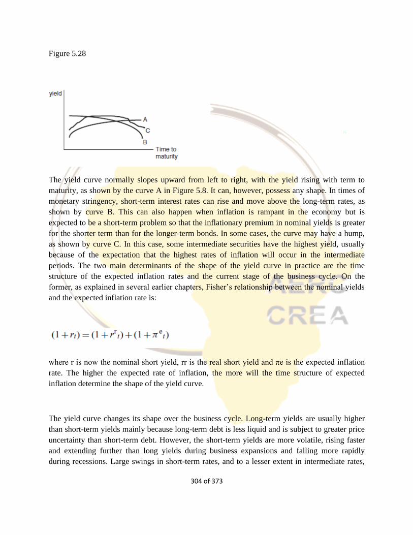
304 of 373

Figure 5.28

The yield curve normally slopes upward from left to right, with the yield rising with term to

maturity, as shown by the curve A in Figure 5.8. It can, however, possess any shape. In times of

monetary stringency, short-term interest rates can rise and move above the long-term rates, as

shown by curve B. This can also happen when inflation is rampant in the economy but is

expected to be a short-term problem so that the inflationary premium in nominal yields is greater

for the shorter term than for the longer-term bonds. In some cases, the curve may have a hump,

as shown by curve C. In this case, some intermediate securities have the highest yield, usually

because of the expectation that the highest rates of inflation will occur in the intermediate

periods. The two main determinants of the shape of the yield curve in practice are the time

structure of the expected inflation rates and the current stage of the business cycle. On the

former, as explained in several earlier chapters, Fisher’s relationship between the nominal yields

and the expected inflation rate is:

where r is now the nominal short yield, rr is the real short yield and πe is the expected inflation

rate. The higher the expected rate of inflation, the more will the time structure of expected

inflation determine the shape of the yield curve.

The yield curve changes its shape over the business cycle. Long-term yields are usually higher

than short-term yields mainly because long-term debt is less liquid and is subject to greater price

uncertainty than short-term debt. However, the short-term yields are more volatile, rising faster

and extending further than long yields during business expansions and falling more rapidly

during recessions. Large swings in short-term rates, and to a lesser extent in intermediate rates,

305 of 373

together with relatively narrow movements in long-term rates, cause a change in the shape of the

yield curve over the course of a business cycle.

A sharp increase in short-term rates frequently occurs near the peak of a business expansion

because of a combination of factors, most often including a strong demand for short-term credit,

restrictive effects of monetary policies on the supply of credit, and changing investor

expectations. Depending upon the intensity of these forces, the yield curve will be relatively flat,

have a slight downward slope, or show a steep negative slope. As short rates fall absolutely and

relative to long yields during the ensuing economic slowdown, the yield curve tends to regain its

positive slope, acquiring its steepest slope near the cyclical trough. As the economy recovers and

economic activity picks up, short rates again rise faster than long yields, and the yield curve

tends to acquire a more moderate slope. Since the yield curve plots the nominal rather than the

real rate of interest, and the nominal rate includes the expected rate of inflation, the dominant

element of the shape and shifts in the yield curve is often the term structure of the expected rate

of inflation.

There are basically three main theories on the term structure of interest rates. These are:

The expectations hypothesis, first formulated by Irving Fisher. This theory is the relevant one for

financially developed markets and is supported by most empirical studies.

The segmented markets theory, with Culbertson as its major proponent.

The preferred habitat hypothesis.

Expectations hypothesis

Irving Fisher in The Theory of Interest (1930, pp. 399–451) considered the rate of return or

yields on securities that differ only in terms of their maturity. His approach assumes that:

All borrowers and lenders have perfect foresight and know future interest rates and asset prices

with certainty, so that there is no risk. An alternative assumption to this is that, while there is

uncertainty of yields, the borrowers and lenders are risk neutral and form rational expectations

about the future short rates.

There are no transactions costs in switching from money into securities and vice versa.

306 of 373

The financial markets are efficient.

A market is said to be efficient if it clears (i.e. demand equals supply) instantly and prices reflect

all available information. In such a market, any opportunities for superior profits are instantly

eliminated. By comparison, a perfect market assumes perfect competition among traders and

efficient markets. Fisher’s assumptions specify an efficient market, which need not have perfect

competition, so that it need not be a perfect one.

Investors are assumed to maximize their expected utility, subject to the relevant constraints.

However, under assumption (i), this is synonymous with the maximization of the expected return

to the portfolio. Under assumptions (i) and (ii), a lender wishing to make a loan for n periods will

be indifferent between an n-period loan or a succession of n one-period loans only if the overall

return were the same in both cases. Under assumption (iii), with all investors acting on this basis,

the market yields will be such as to ensure this indifference.

Expectations hypothesis, complete markets and forward rates

Assume that the financial sector has complete markets, so that there exist markets for long loans

of all possible maturities, as well as for spot and forward one-period loans. With the current

period as t, the yield (per period) on an (i+1)-period loan was designated as tRt+i, while that on a

one period loan for the (i+1)th period was trft+i, i =0,1, . . .,n, where n+1 is the longest maturity

available in the market. Hence, trt is the (spot) yield on a loan for the first period; trft+1 is the

forward yield on a loan for the second period; and so on. An (i+1)-period loan of $1 will pay the

lender (l +tRt+i)i+1 at the end of the (i+1)th period. The series of (i+1) loans starting with a

principal of $1 for one-period at a time will pay him [(1+trt) (1+trft+1) . . . (1+trft+i)] at the end

of the (i+1)th period.

Under the above three assumptions, the lender will be indifferent between the two types of loans

if the total amount repaid to him after n + 1 periods is identical. With all investors exhibiting this

behavior, efficient markets under certainty ensure that:

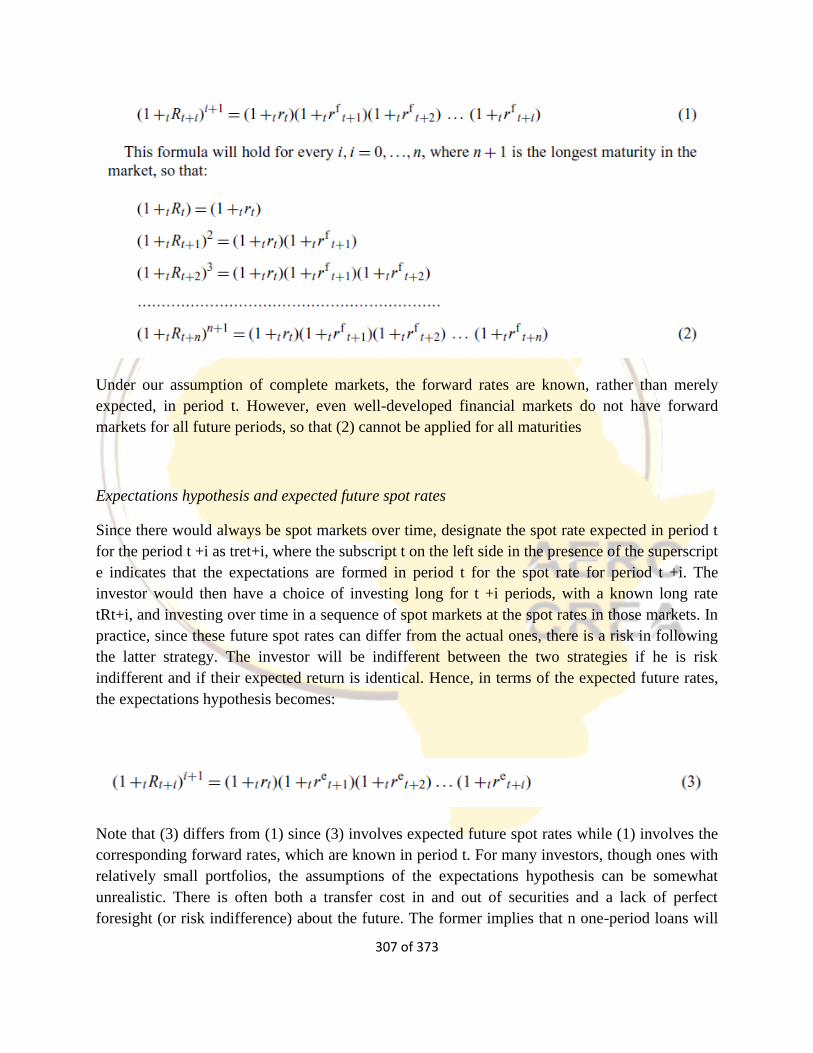
307 of 373

Under our assumption of complete markets, the forward rates are known, rather than merely

expected, in period t. However, even well-developed financial markets do not have forward

markets for all future periods, so that (2) cannot be applied for all maturities

Expectations hypothesis and expected future spot rates

Since there would always be spot markets over time, designate the spot rate expected in period t

for the period t +i as tret+i, where the subscript t on the left side in the presence of the superscript

e indicates that the expectations are formed in period t for the spot rate for period t +i. The

investor would then have a choice of investing long for t +i periods, with a known long rate

tRt+i, and investing over time in a sequence of spot markets at the spot rates in those markets. In

practice, since these future spot rates can differ from the actual ones, there is a risk in following

the latter strategy. The investor will be indifferent between the two strategies if he is risk

indifferent and if their expected return is identical. Hence, in terms of the expected future rates,

the expectations hypothesis becomes:

Note that (3) differs from (1) since (3) involves expected future spot rates while (1) involves the

corresponding forward rates, which are known in period t. For many investors, though ones with

relatively small portfolios, the assumptions of the expectations hypothesis can be somewhat

unrealistic. There is often both a transfer cost in and out of securities and a lack of perfect

foresight (or risk indifference) about the future. The former implies that n one-period loans will

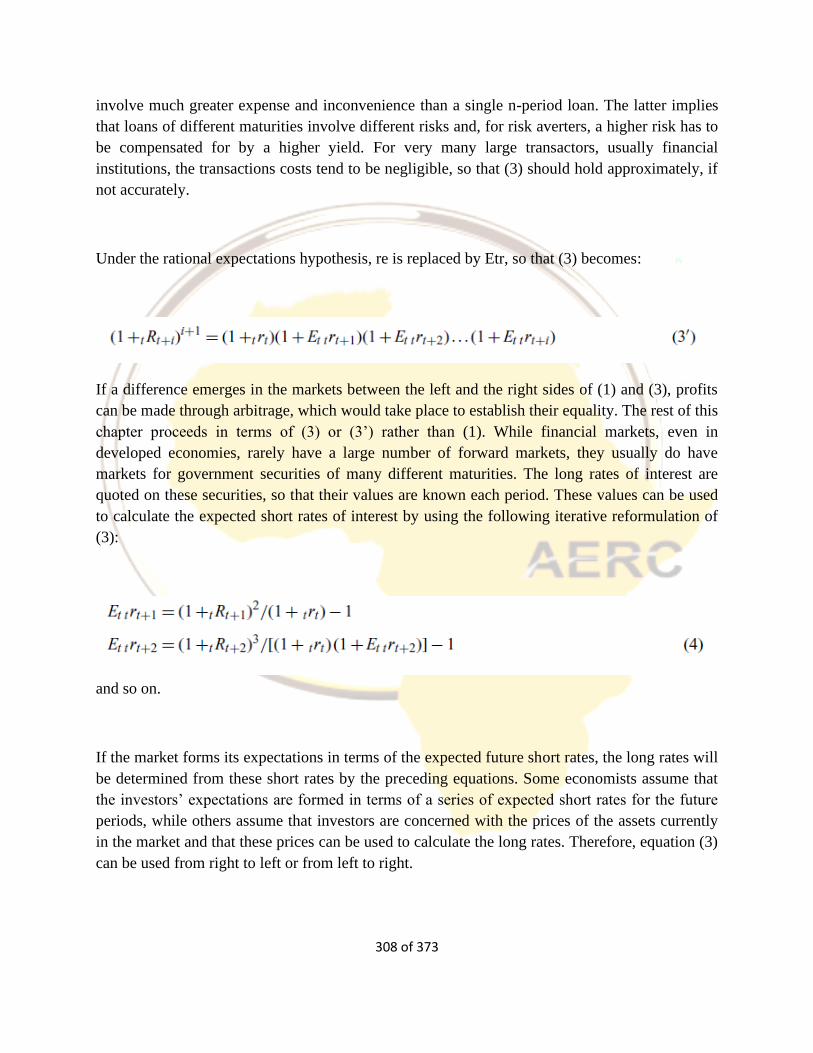
308 of 373

involve much greater expense and inconvenience than a single n-period loan. The latter implies

that loans of different maturities involve different risks and, for risk averters, a higher risk has to

be compensated for by a higher yield. For very many large transactors, usually financial

institutions, the transactions costs tend to be negligible, so that (3) should hold approximately, if

not accurately.

Under the rational expectations hypothesis, re is replaced by Etr, so that (3) becomes:

If a difference emerges in the markets between the left and the right sides of (1) and (3), profits

can be made through arbitrage, which would take place to establish their equality. The rest of this

chapter proceeds in terms of (3) or (3’) rather than (1). While financial markets, even in

developed economies, rarely have a large number of forward markets, they usually do have

markets for government securities of many different maturities. The long rates of interest are

quoted on these securities, so that their values are known each period. These values can be used

to calculate the expected short rates of interest by using the following iterative reformulation of

(3):

and so on.

If the market forms its expectations in terms of the expected future short rates, the long rates will

be determined from these short rates by the preceding equations. Some economists assume that

the investors’ expectations are formed in terms of a series of expected short rates for the future

periods, while others assume that investors are concerned with the prices of the assets currently

in the market and that these prices can be used to calculate the long rates. Therefore, equation (3)

can be used from right to left or from left to right.

309 of 373

Long rates as geometric averages of short rates

According to (3), the long rates are geometric averages of the short rates of interest. This implies

that:

If the short interest rates are expected to be identical, the long rate will equal the short rate.

If the short interest rates are expected to rise, the long rates will lie above the current short rates.

If the short interest rates are expected to decline, the long rates will be less than the current short

rate.

The long rate, being an average of the short rates, will fluctuate less than the short rate.

In principle, any pattern of expected future short rates is possible, with the result that some long

rates may be less and some greater than the current spot rate, so that the yield curve may have

any shape whatever.

The assumptions of the expectations hypothesis may not always hold for all agents in the market,

which encompasses both households and firms. However, developed financial economies tend to

be competitive and efficient. Therefore, the expectations hypothesis will hold if the credit

markets have sufficient numbers of participants who behave according to the assumptions of

perfect foresight (or of rational expectations and risk indifference) and zero variable transfer

costs between securities and money. These assumptions tend to be valid at least for large

financial institutions operating in the developed economies. Hence, the expectations hypothesis

should be more or less valid for developed financial markets.

Liquidity preference version of the expectations hypothesis

Both the n-period loan and a series of n one-period loans involve risks, though of different kinds.

The n one-period loans involve the possibility that the future spot rates will turn out to be lower

than the expected forward rates or the n-period long rate. This is an income loss. But the n-period

loan – that is, purchase of a bond maturing after n periods – involves the possibility that the

lender may need his funds somewhat sooner and have to sell the bond before it matures. Such a

sale may involve a capital loss, especially in the absence of a secondary market for loans. There

is also the possibility that more profitable opportunities may turn up and have to be foregone if

the funds are already loaned up for a long period.

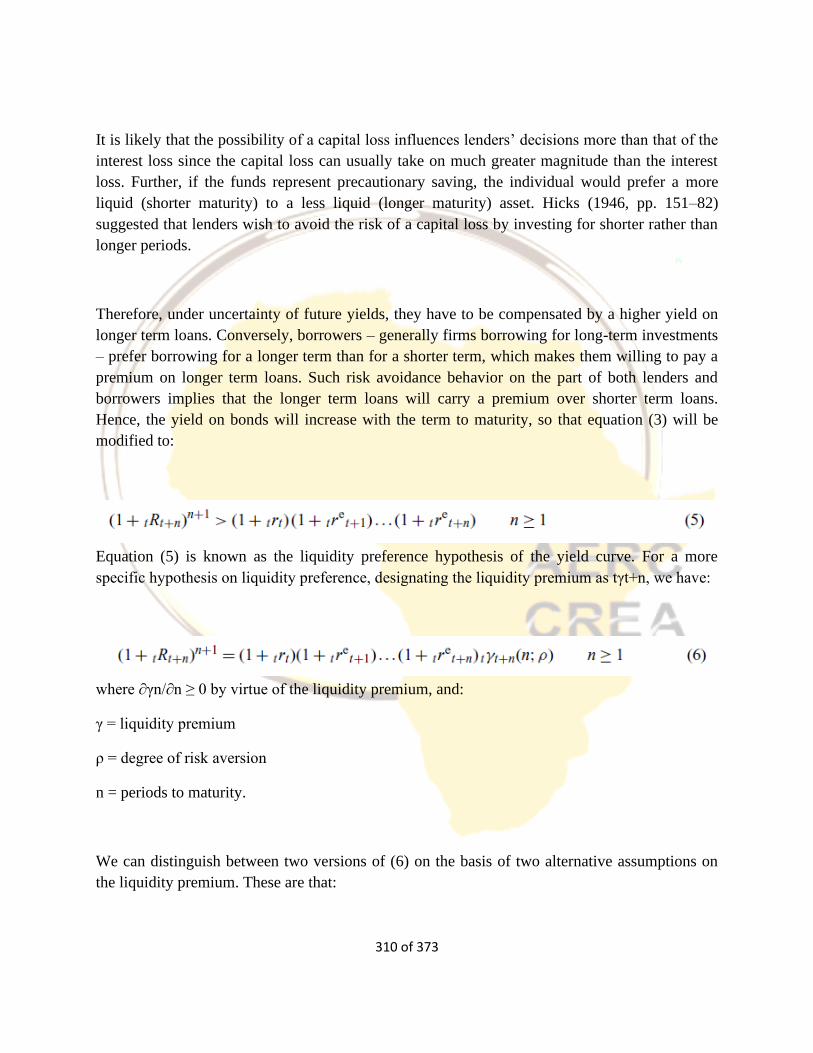
310 of 373

It is likely that the possibility of a capital loss influences lenders’ decisions more than that of the

interest loss since the capital loss can usually take on much greater magnitude than the interest

loss. Further, if the funds represent precautionary saving, the individual would prefer a more

liquid (shorter maturity) to a less liquid (longer maturity) asset. Hicks (1946, pp. 151–82)

suggested that lenders wish to avoid the risk of a capital loss by investing for shorter rather than

longer periods.

Therefore, under uncertainty of future yields, they have to be compensated by a higher yield on

longer term loans. Conversely, borrowers – generally firms borrowing for long-term investments

– prefer borrowing for a longer term than for a shorter term, which makes them willing to pay a

premium on longer term loans. Such risk avoidance behavior on the part of both lenders and

borrowers implies that the longer term loans will carry a premium over shorter term loans.

Hence, the yield on bonds will increase with the term to maturity, so that equation (3) will be

modified to:

Equation (5) is known as the liquidity preference hypothesis of the yield curve. For a more

specific hypothesis on liquidity preference, designating the liquidity premium as tγt+n, we have:

where ∂γn/∂n ≥ 0 by virtue of the liquidity premium, and:

γ = liquidity premium

ρ = degree of risk aversion

n = periods to maturity.

We can distinguish between two versions of (6) on the basis of two alternative assumptions on

the liquidity premium. These are that:

311 of 373

(i) The liquidity premium is constant at γ per period, so that tγt+i = iγ . While there is no

particular intuitive justification for making this assumption, it is analytically convenient and, as

seen later in this chapter, is made in many empirical studies. It reduces (6) to:

Equation (7) with a constant per period risk premium is sometimes called the strong form of the

expectations hypothesis with a liquidity premium.

(ii) The per period liquidity premium varies with the term to maturity and, moreover, may not be

constant over time, e.g. over the business cycle, so that (6) does not simplify to (7). This is

sometimes called the weak form of the expectations hypothesis with a liquidity premium.

Estimation of this form requires specification of the determinants of the liquidity premium.

Compared with these weak and strong forms of the expectations hypotheses, the original form

(3) of this hypothesis without a liquidity premium is known as the pure form of the expectations

hypothesis.

Segmented markets hypothesis

If the uncertainty in the loan market is extremely severe or if lenders and borrowers have

extremely high-risk aversion, each lender will attempt to lend for the exact period for which he

has spare funds and each borrower will borrow for the exact period for which he needs funds. In

this extreme case, the overall credit market will be split into a series of segments or separate

markets based on the maturity of loans, without any substitution by either borrowers or lenders

among the different markets. Therefore, the yields in any one market for a given maturity cannot

influence the yields in another market for another maturity. Hence, there would not be any

particular relationship such as (3) or (6) between the long and the short rates, and the yield curve

could have any shape whatever. This is the basic element of the segmented markets theory: the

market is segmented into a set of independent markets.

Culbertson (1957) stressed this possibility as a major, though not the only, determinant of the

term structure of interest rates. Culbertson also argued that the lender rarely knows in advance

312 of 373

exactly when he will need his funds again and will prefer to make loans for shorter terms rather

than longer ones, the former being the more liquid of the two. If the supply of short-term debt

instruments is not sufficient to meet this demand for liquidity at a rate of interest equal to the

long-term rate, the short-term rate will be less than the long-term rate. Further, the supply of

short-term instruments is generally limited since lenders will not finance long-term investment

with short-term borrowing. Therefore, the short-term yield will be less than the long-term yield,

ceteris paribus.

The segmented markets hypothesis is more likely to be applicable in the absence of developed

financial markets, including secondary markets for securities, and sophisticated investors. It may

therefore be somewhat more valid for financially underdeveloped markets than for developed

ones.

Preferred habitat hypothesis

The preferred habitat hypothesis was proposed by Modigliani and Sutch (1966, 1967), and

represents a compromise between the expectations hypothesis of perfect substitutability and the

segmented markets hypothesis of zero substitution between loans of different maturities.

Modigliani and Sutch argued that lenders would prefer to lend for periods for which they can

spare the funds and borrowers would prefer to borrow the funds for periods for which they need

the funds. However, each would be willing to substitute other maturities, depending upon their

willingness to take risks and the opportunities provided by the market to transfer easily among

different maturities. Bonds maturing close together would usually be fairly good substitutes and

have similar risk premiums.

This would be especially so for bonds at the longer end of the maturity spectrum. Therefore, in

well-developed financial markets, a high degree of substitutability would exist among different

maturities, but without these necessarily becoming perfect substitutes. Hence, while the yields on

different maturities would be interrelated to a considerable extent, there would also continue to

exist some variation in yields among the different maturities.

Implications of the term structure hypotheses for monetary policy

The expectations theory and the segmented markets theory have significantly different

implications for the management of the public debt and for the operation of monetary policy. The

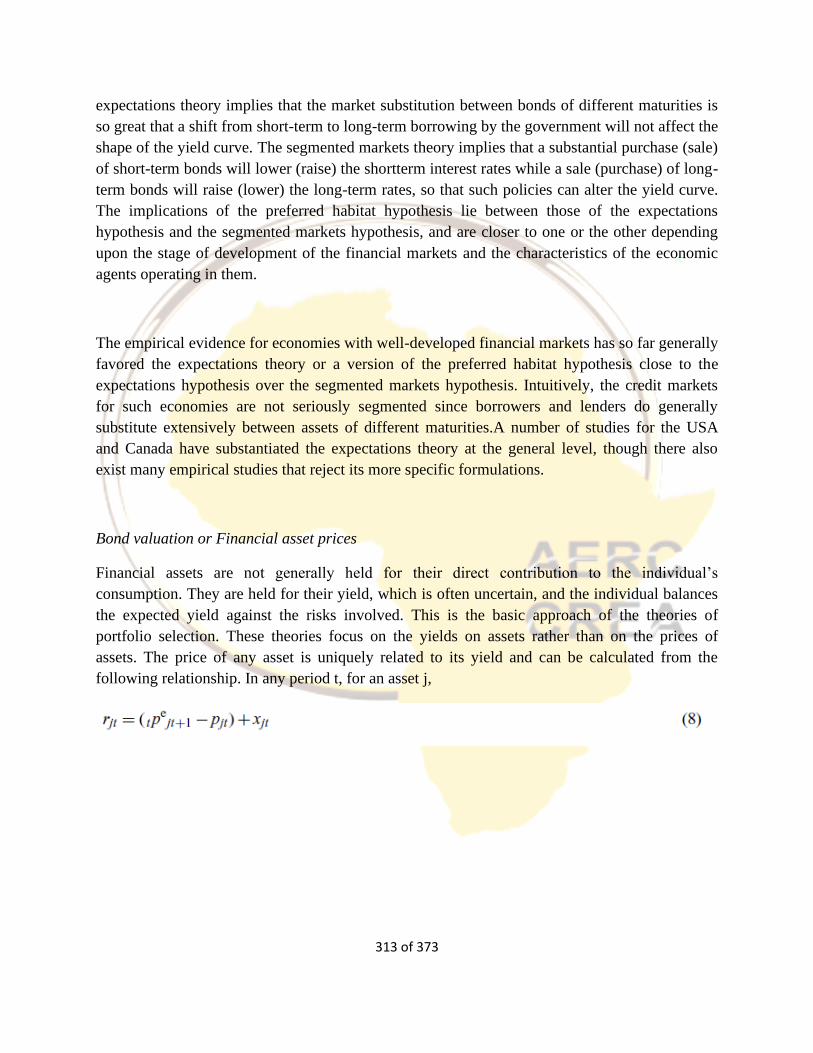
313 of 373

expectations theory implies that the market substitution between bonds of different maturities is

so great that a shift from short-term to long-term borrowing by the government will not affect the

shape of the yield curve. The segmented markets theory implies that a substantial purchase (sale)

of short-term bonds will lower (raise) the shortterm interest rates while a sale (purchase) of long-

term bonds will raise (lower) the long-term rates, so that such policies can alter the yield curve.

The implications of the preferred habitat hypothesis lie between those of the expectations

hypothesis and the segmented markets hypothesis, and are closer to one or the other depending

upon the stage of development of the financial markets and the characteristics of the economic

agents operating in them.

The empirical evidence for economies with well-developed financial markets has so far generally

favored the expectations theory or a version of the preferred habitat hypothesis close to the

expectations hypothesis over the segmented markets hypothesis. Intuitively, the credit markets

for such economies are not seriously segmented since borrowers and lenders do generally

substitute extensively between assets of different maturities.A number of studies for the USA

and Canada have substantiated the expectations theory at the general level, though there also

exist many empirical studies that reject its more specific formulations.

Bond valuation or Financial asset prices

Financial assets are not generally held for their direct contribution to the individual’s

consumption. They are held for their yield, which is often uncertain, and the individual balances

the expected yield against the risks involved. This is the basic approach of the theories of

portfolio selection. These theories focus on the yields on assets rather than on the prices of

assets. The price of any asset is uniquely related to its yield and can be calculated from the

following relationship. In any period t, for an asset j,

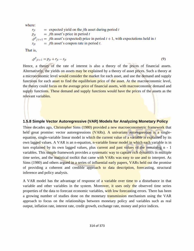
314 of 373

Hence, a theory of the rate of interest is also a theory of the prices of financial assets.

Alternatively, the yields on assets may be explained by a theory of asset prices. Such a theory at

a microeconomic level would consider the market for each asset, and use the demand and supply

functions for each asset to find the equilibrium price of the asset. At the macroeconomic level,

the theory could focus on the average price of financial assets, with macroeconomic demand and

supply functions. These demand and supply functions would have the prices of the assets as the

relevant variables.

1.5.8 Simple Vector Autoregressive (VAR) Models for Analyzing Monetary Policy

Three decades ago, Christopher Sims (1980) provided a new macroeconometric framework that

held great promise: vector autoregressions (VARs). A univariate autoregression is a single-

equation, single-variable linear model in which the current value of a variable is explained by its

own lagged values. A VAR is an n-equation, n-variable linear model in which each variable is in

turn explained by its own lagged values, plus current and past values of the remaining n - 1

variables. This simple framework provides a systematic way to capture rich dynamics in multiple

time series, and the statistical toolkit that came with VARs was easy to use and to interpret. As

Sims (1980) and others argued in a series of influential early papers, VARs held out the promise

of providing a coherent and credible approach to data description, forecasting, structural

inference and policy analysis.

A VAR model has the advantage of response of a variable over time to a disturbance in that

variable and other variables in the system. Moreover, it uses only the observed time series

properties of the data to forecast economic variables, with low forecasting errors. There has been

a growing number of studies done on the monetary transmission mechanism using the VAR

approach to focus on the relationships between monetary policy and variables such as real

output, inflation rate, interest rate, credit growth, exchange rate, money and price indices.

315 of 373

Basic VAR as Tool for Monetary Policy Analysis

What, precisely, is the effect of a 100-basis-point hike in the federal funds interest rate on the

rate of inflation one year hence? How big an interest rate cut is needed to offset an expected half

percentage point rise in the unemployment rate? How well does the Phillips curve predict

inflation? What fraction of the variation in inflation in the past 40 years is due to monetary

policy as opposed to external shocks? Many macroeconomists like to think they know the

answers to these and similar questions, perhaps with a modest range of uncertainty. In the next

two sections, we take a quantitative look at these and related questions using several three-

variable VARs estimated using quarterly U.S. data on the rate of price inflation (iit), the

unemployment rate (ut) and the interest rate (Re, specifically, the federal funds rate) from

1960:I-2000:IV.2 First, we construct and examine these models as a way to display the VAR

toolkit; criticisms are reserved for the next section.

VARs come in three varieties: reduced form, recursive and structural. A reduced form VAR

expresses each variable as a linear function of its own past values, the past values of all other

variables being considered and a serially uncorrelated error term. Thus, in our example, the VAR

involves three equations: current unemployment as a function of past values of unemployment,

inflation and the interest rate; inflation as a function of past values of inflation, unemployment

and the interest rate; and similarly for the interest rate equation. Each equation can be estimated

by ordinary least squares regression. The number of lagged values to include in each equation

can be determined by a number of different methods, and we will use four lags in our examples.

The error terms in these regressions are the "surprise" movements in the variables after taking its

past values into account. If the different variables are correlated with each other-as they typically

are in macroeconomic applications-then the error terms in the reduced form model will also be

correlated across equations.

A recursive VAR constructs the error terms in each regression equation to be uncorrelated with

the error in the preceding equations. This is done by judiciously including some

contemporaneous values as regressors. Consider a three-variable VAR, ordered as 1) inflation, 2)

the unemployment rate, and 3) the interest rate. In the first equation of the corresponding

recursive VAR, inflation is the dependent variable, and the regressors are lagged values of all

three variables. In the second equation, the unemployment rate is the dependent variable, and the

regressors are lags of all three variables plus the current value of the inflation rate. The interest

rate is the dependent variable in the third equation, and the regressors are lags of all three

variables, the current value of the inflation rate plus the current value of the unemployment rate.

Estimation of each equation by ordinary least squares produces residuals that are uncorrelated

across equations. Evidently, the results depend on the order of the variables: changing the order

changes the VAR equations, coefficients, and residuals, and there are n! recursive VARs

representing all possible orderings.

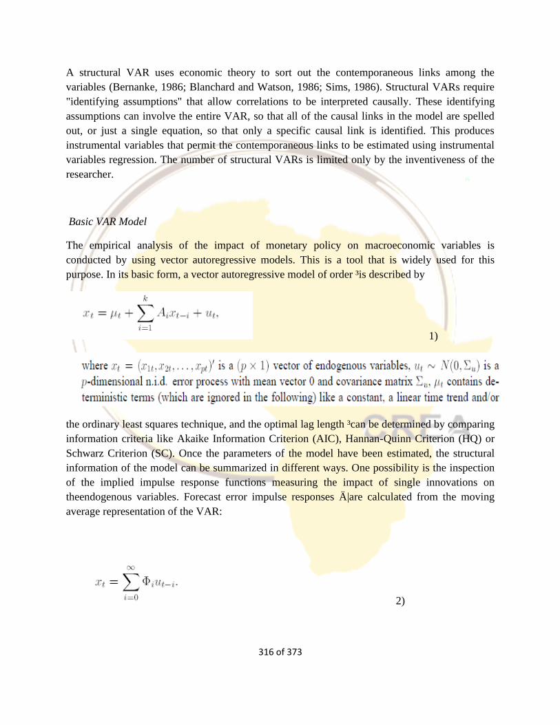
316 of 373

A structural VAR uses economic theory to sort out the contemporaneous links among the

variables (Bernanke, 1986; Blanchard and Watson, 1986; Sims, 1986). Structural VARs require

"identifying assumptions" that allow correlations to be interpreted causally. These identifying

assumptions can involve the entire VAR, so that all of the causal links in the model are spelled

out, or just a single equation, so that only a specific causal link is identified. This produces

instrumental variables that permit the contemporaneous links to be estimated using instrumental

variables regression. The number of structural VARs is limited only by the inventiveness of the

researcher.

Basic VAR Model

The empirical analysis of the impact of monetary policy on macroeconomic variables is

conducted by using vector autoregressive models. This is a tool that is widely used for this

purpose. In its basic form, a vector autoregressive model of order ³is described by

1)

the ordinary least squares technique, and the optimal lag length ³can be determined by comparing

information criteria like Akaike Information Criterion (AIC), Hannan-Quinn Criterion (HQ) or

Schwarz Criterion (SC). Once the parameters of the model have been estimated, the structural

information of the model can be summarized in different ways. One possibility is the inspection

of the implied impulse response functions measuring the impact of single innovations on

theendogenous variables. Forecast error impulse responses Ä|are calculated from the moving

average representation of the VAR:

2)

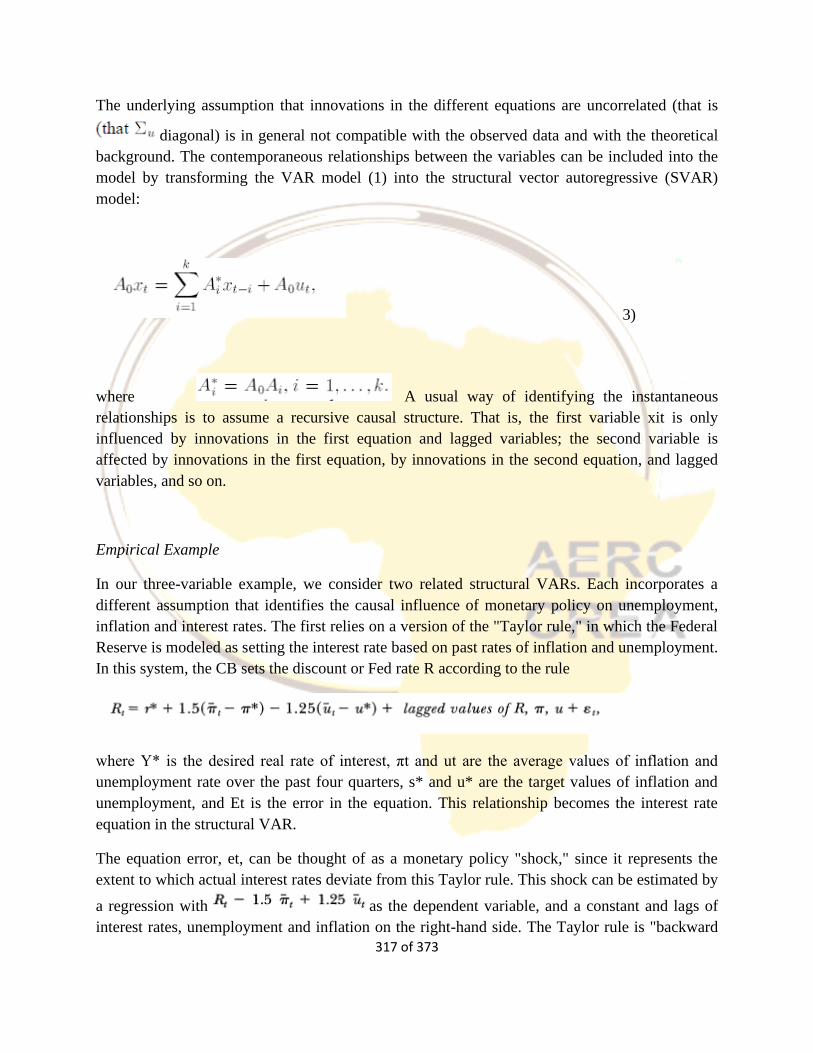
317 of 373

The underlying assumption that innovations in the different equations are uncorrelated (that is

diagonal) is in general not compatible with the observed data and with the theoretical

background. The contemporaneous relationships between the variables can be included into the

model by transforming the VAR model (1) into the structural vector autoregressive (SVAR)

model:

3)

where A usual way of identifying the instantaneous

relationships is to assume a recursive causal structure. That is, the first variable xit is only

influenced by innovations in the first equation and lagged variables; the second variable is

affected by innovations in the first equation, by innovations in the second equation, and lagged

variables, and so on.

Empirical Example

In our three-variable example, we consider two related structural VARs. Each incorporates a

different assumption that identifies the causal influence of monetary policy on unemployment,

inflation and interest rates. The first relies on a version of the "Taylor rule," in which the Federal

Reserve is modeled as setting the interest rate based on past rates of inflation and unemployment.

In this system, the CB sets the discount or Fed rate R according to the rule

where Y* is the desired real rate of interest, πt and ut are the average values of inflation and

unemployment rate over the past four quarters, s* and u* are the target values of inflation and

unemployment, and Et is the error in the equation. This relationship becomes the interest rate

equation in the structural VAR.

The equation error, et, can be thought of as a monetary policy "shock," since it represents the

extent to which actual interest rates deviate from this Taylor rule. This shock can be estimated by

a regression with as the dependent variable, and a constant and lags of

interest rates, unemployment and inflation on the right-hand side. The Taylor rule is "backward

318 of 373

looking" in the sense that the Fed reacts to past information (πt and ut are averages of the past

four quarters of inflation and unemployment), and several researchers have argued that Fed

behavior is more appropriately described by forward-looking behavior. Because of this, we

consider another variant of the model in which the Fed reacts to forecasts of inflation and

unemployment four quarters in the future. This Taylor rule has the same form as the rule above,

but with πt and ut replaced by four-quarter ahead forecasts computed from the reduced form

VAR.

Putting the Three-Variable VAR Through Its Paces The different versions of the inflation-

unemployment-interest rate VAR are put through their paces by applying them to the four

macroeconometric tasks. First, the reduced form VAR and a recursive VAR are used to

summarize the comovements of these three series. Second, the reduced form VAR is used to

forecast the variables, and its performance is assessed against some alternative benchmark

models. Third, the two different structural VARs are used to estimate the effect of a policy-

induced surprise move in the federal funds interest rate on future rates of inflation and

unemployment. Finally, we discuss how the structural VAR could be used for policy analysis.

Data Description Standard practice in VAR analysis is to report results from Granger-causality

tests, impulse responses and forecast error variance decompositions. These statistics are

computed automatically (or nearly so) by many econometrics packages (RATS, Eviews, TSP and

others). Because of the complicated dynamics in the VAR, these statistics are more informative

than are the estimated VAR regression coefficients or R2 statistics, which typically go

unreported. Granger-causality statistics examine whether lagged values of one variable help to

predict another variable. For example, if the unemployment rate does not help predict inflation,

then the coefficients on the lags of unemployment will all be zero in the reduced-form inflation

equation. Panel A of Table 1 summarizes the Granger-causality results for the three-variable

VAR. It shows the p-values associated with the Fstatistics for testing whether the relevant sets of

coefficients are zero. The unemployment rate helps to predict inflation at the 5 percent

significance level (the p-value is 0.02, or 2 percent), but the federal funds interest rate does not

(the p-value is 0.27). Inflation does not help to predict the unemployment rate, but the federal

funds rate does. Both inflation and the unemployment rates help predict the federal funds interest

rate.

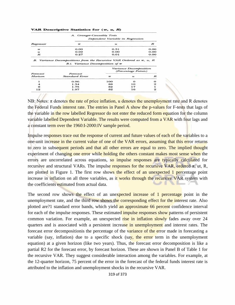
319 of 373

NB: Notes: π denotes the rate of price inflation, u denotes the unemployment rate and R denotes

the Federal Funds interest rate. The entries in Panel A show the p-values for F-tests that lags of

the variable in the row labelled Regressor do not enter the reduced form equation for the column

variable labelled Dependent Variable. The results were computed from a VAR with four lags and

a constant term over the 1960:I-2000:IV sample period.

Impulse responses trace out the response of current and future values of each of the variables to a

one-unit increase in the current value of one of the VAR errors, assuming that this error returns

to zero in subsequent periods and that all other errors are equal to zero. The implied thought

experiment of changing one error while holding the others constant makes most sense when the

errors are uncorrelated across equations, so impulse responses are typically calculated for

recursive and structural VARs. The impulse responses for the recursive VAR, ordered π, ut, R,

are plotted in Figure 1. The first row shows the effect of an unexpected 1 percentage point

increase in inflation on all three variables, as it works through the recursive VAR system with

the coefficients estimated from actual data.

The second row shows the effect of an unexpected increase of 1 percentage point in the

unemployment rate, and the third row shows the corresponding effect for the interest rate. Also

plotted are?1 standard error bands, which yield an approximate 66 percent confidence interval

for each of the impulse responses. These estimated impulse responses show patterns of persistent

common variation. For example, an unexpected rise in inflation slowly fades away over 24

quarters and is associated with a persistent increase in unemployment and interest rates. The

forecast error decompositionis the percentage of the variance of the error made in forecasting a

variable (say, inflation) due to a specific shock (say, the error term in the unemployment

equation) at a given horizon (like two years). Thus, the forecast error decomposition is like a

partial R2 for the forecast error, by forecast horizon. These are shown in Panel B of Table 1 for

the recursive VAR. They suggest considerable interaction among the variables. For example, at

the 12-quarter horizon, 75 percent of the error in the forecast of the federal funds interest rate is

attributed to the inflation and unemployment shocks in the recursive VAR.

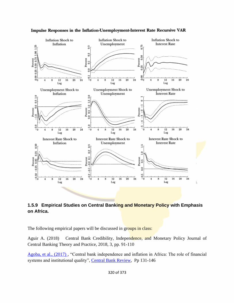
320 of 373

1.5.9 Empirical Studies on Central Banking and Monetary Policy with Emphasis

on Africa.

The following empirical papers will be discussed in groups in class:

Aguir A. (2018) Central Bank Credibility, Independence, and Monetary Policy Journal of

Central Banking Theory and Practice, 2018, 3, pp. 91-110

Agoba, et al., (2017) , “Central bank independence and inflation in Africa: The role of financial

systems and institutional quality”, Central Bank Review, Pp 131-146

321 of 373

Ftiti et al., (2017), “Time-inconsistency and expansionary business cycle theories: What does

matter for the central bank independence–inflation relationship?” Economic Modelling, Vol. 67,

Pp 215-227

Creamer, K, and Botha T. (2017), “Assessing nominal GDP targeting in the South African

context” Central Bank Review, Vol 17, Pp 1-10

And more

Review and Discussion Questions

Why has the use of changes in reserve requirements as a tool of monetary policy been largely

abandoned in Western economies? What were the reasons for the virtual elimination of reserve

requirements? Is there a case for their revival and usage as a tool of monetary policy in the

context of the country you live in? In LDCs?

How do central banks manage interest rates in your country and one other country of your

choice? What consequences for output fluctuations can the central bank expect from targeting

interest rates?

The monetary sector has become increasingly unstable in recent years. Does this mean that the

monetary authority should stay with the pursuit of interest-rate targets and leave the money

supply alone?

Can central banks pursue and achieve multiple goals or must they be confined solely to fighting

inflation? What goals are embedded in the Taylor rule? Discuss.

What is the lender-of-last-resort function of the central bank in modern economies? What is its

justification? Should commercial bank borrowing from the central bank be a privilege or a right?

Discuss.

322 of 373

Explain how the monetary and real factors enter into the determination of the interest rates in the

short run and in the long run.

Compare and contrast the liquidity preference and loanable funds theories of the rate of interest.

Discuss their implications for monetary policies intended to maintain full employment.

Keynes asserted that there is no such thing as a non-monetary theory of the rate of interest and

that the rate of interest is uniquely determined by the demand and supply of money.

Explain Keynes’s reasons for this view. Compare this view with those of the traditional classical

and modern classical schools.

The yield curve shows the relationship between the yields of high-grade securities that differ

only in the term to maturity. Sometimes the curve rises, sometimes it falls and sometimes it is

flat. Present the main reasons for these different shapes.

“On the basis of recent empirical studies, the expectations hypothesis with efficient markets and

rational expectations does not seem to explain the term structure of interest rates.” Discuss.

Present the findings of at least one such study and discuss the potential reasons for this failure.

Can the central bank change the shape of the yield curve through changes in (a) the term

structure of government bonds and (b) variations over time in monetary aggregates?

Discuss.

For your country, what is the current shape of the yield curve? Explain this shape.

Assuming that the expectations theory of the yield curve is correct, derive from your data on the

yield curve the expected future spot rates for the next twelve months.

323 of 373

If your economy has forward markets for this period, compare the forward short rates with your

derived expected future spot rates, and explain the reasons for any differences.

324 of 373

1.6 MONEY IN THE OPEN ECONOMY

Introduction

In this section, I shall focus on the role money plays in determining a country’s Balance of

Payments and exchange rate. You will soon know that the impact of monetary policy in an open

economy depends on the nature of the exchange rate system in operation. This is because in this

section, we shall consider the impact of changes in the money stock on nominal income in a

fixed exchange rate system and showed that, with fixed exchange rates and mobile capital,

monetary policy has only a temporary impact on the level of income and, in the longer run, is

completely ineffective. On the other hand, with freely floating exchange rates and mobile capital,

monetary policy is more effective than in the closed economy case.

Before we discuss the issues relating to monetary policy in the open economy, I shall walk you

through the factors that determine the exchange rate in both the short-run and long run. As you

know, the exchange rate plays a vital role in a country's level of foreign trade, which is critical to

most free market economies in the world. Mostly, an exchange rate is used as one of the most

important determinants of a country's relative level of economic health. Due to its significance in

international trade, many researchers have tried to develop models which build relationships

between forces that determine the magnitude and movement of the exchange rates. The

following are the specific learning objectives for this section:

Learning Objectives

Students should be able to do the following at the end of the class:

Explain and illustrate the factors that affect the exchange rate determination in the short run

and long run.

Explain monetary and portfolio approaches to Balance of Payments (BOPs) and exchange rate

determination as well as BOPs Determination Approaches

Describe the link between money Money and BOP Adjustments

Explain and illustrate the effect of monetary policy under alternative exchange rate regimes

Compare and contrast the arguments for and against monetary policy coordination amongst

countries

1.6.1 Short Run and Long Run Determination of Exchange Rate; Portfolio Asset

Approach; Balance of Payments (BOP) Determination Approaches

Exchange Rate Determination

The price of one currency in terms of another is called the exchange rate. As you may know,

exchange rates in all countries exhibit so much volatility. The exchange rate affects the economy

and our daily lives, because when the U.S. dollar , for example, becomes more valuable relative

to foreign currencies, foreign goods become cheaper for Americans, and American goods

become more expensive for foreigners. When the U.S. dollar falls in value, foreign goods

become more expensive for Americans, and American goods become cheaper for foreigners.

325 of 373

Fluctuations in the exchange rate also affect both inflation and output, and are an important

concern to monetary policymakers. When the U.S. dollar falls in value, the higher prices of

imported goods feed directly into a higher price level and inflation. At the same time, a declining

U.S. dollar, which makes domestic goods cheaper for foreigners, increases the demand for

domestic. goods and leads to higher production and output.

Exchange Rates in the Long Run

Like the price of any good or asset in a free market, exchange rates are determined by the

interaction of supply and demand. To simplify our analysis of exchange rates in a free market,

we divide it into two parts. First, we examine how exchange rates are determined in the long run;

then we use our knowledge of the long-run determinants of exchange rates to help us understand

how they are determined in the short run.

Law of One Price

The starting point for understanding how exchange rates are determined is a simple idea called

the law of one price: If two countries produce an identical good, and transportation costs and

trade barriers are very low, the price of the good should be the same throughout the world, no

matter which country produces it. Suppose that American steel costs $100 per ton and identical

Japanese steel costs 10,000 yen per ton. For the law of one price to hold, the exchange rate

between the yen and the dollar must be 100 yen per dollar ($0.01 per yen), so that one ton of

American steel sells for 10,000 yen in Japan (the price of Japanese steel) and one ton of Japanese

steel sells for $100 in the United States (the price of U.S. steel). If the exchange rate were 200

yen to the dollar, Japanese steel would sell for $50 per ton in the United States, or half the price

of American steel, and American steel would sell for 20,000 yen per ton in Japan, twice the price

of Japanese steel.

Because American steel would be more expensive than Japanese steel in both countries and

because American steel is identical to Japanese steel, the demand for American steel would go to

zero. Given a fixed dollar price for American steel, the resulting excess supply of American steel

would be eliminated only if the exchange rate fell to 100 yen per dollar, making the prices of

American steel and Japanese steel the same in both countries.

Theory of Purchasing Power Parity

One of the most prominent theories of how exchange rates are determined is the theory of

purchasing power parity (PPP). It states that exchange rates between any two currencies will

adjust to reflect changes in the price levels of the two countries. The theory of PPP is simply an

application of the law of one price to national price levels rather than to individual prices.

Suppose that the yen price of Japanese steel rises 10% (to 11,000 yen) relative to the dollar price

of American steel (unchanged at $100). For the law of one price to hold, the exchange rate must

rise to 110 yen to the dollar, a 10% appreciation of the dollar. By applying the law of one price to

the price levels in the two countries, we get the theory of purchasing power parity, which

maintains that if the Japanese price level rises 10% relative to the U.S. price level, the dollar will

appreciate by 10%.

Another way of thinking about purchasing power parity is through a concept called the real

exchange rate, the rate at which domestic goods can be exchanged for foreign goods. In effect,

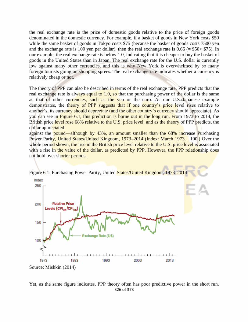
326 of 373

the real exchange rate is the price of domestic goods relative to the price of foreign goods

denominated in the domestic currency. For example, if a basket of goods in New York costs $50

while the same basket of goods in Tokyo costs $75 (because the basket of goods costs 7500 yen

and the exchange rate is 100 yen per dollar), then the real exchange rate is 0.66 (= $50> $75). In

our example, the real exchange rate is below 1.0, indicating that it is cheaper to buy the basket of

goods in the United States than in Japan. The real exchange rate for the U.S. dollar is currently

low against many other currencies, and this is why New York is overwhelmed by so many

foreign tourists going on shopping sprees. The real exchange rate indicates whether a currency is

relatively cheap or not.

The theory of PPP can also be described in terms of the real exchange rate. PPP predicts that the

real exchange rate is always equal to 1.0, so that the purchasing power of the dollar is the same

as that of other currencies, such as the yen or the euro. As our U.S./Japanese example

demonstrates, the theory of PPP suggests that if one country’s price level rises relative to

another’s, its currency should depreciate (and the other country’s currency should appreciate). As

you can see in Figure 6.1, this prediction is borne out in the long run. From 1973 to 2014, the

British price level rose 68% relative to the U.S. price level, and as the theory of PPP predicts, the

dollar appreciated

against the pound—although by 43%, an amount smaller than the 68% increase Purchasing

Power Parity, United States/United Kingdom, 1973–2014 (Index: March 1973 _ 100.) Over the

whole period shown, the rise in the British price level relative to the U.S. price level is associated

with a rise in the value of the dollar, as predicted by PPP. However, the PPP relationship does

not hold over shorter periods.

Figure 6.1: Purchasing Power Parity, United States/United Kingdom, 1973–2014

Source: Mishkin (2014)

Yet, as the same figure indicates, PPP theory often has poor predictive power in the short run.

327 of 373

From early 1985 to the end of 1987, for example, the British price level rose relative to that of

the United States. Instead of appreciating, as predicted by PPP theory, the U.S. dollar actually

depreciated by 40% against the pound. So even though PPP theory provides some guidance as to

the long-run movement of exchange rates, it is not perfect and in the short run is a particularly

poor predictor. What explains the PPP theory’s failure to predict well in the short run?

Criticisms of the Theory of Purchasing Power Parity

The PPP conclusion that exchange rates are determined solely by changes in relative price levels

rests on the assumptions that all goods are identical in both countries and that transportation

costs and trade barriers are very low. When these assumptions are true, the law of one price

states that the relative prices of all these goods (that is, the relative price level between the two

countries) will determine the exchange rate. The assumption that goods are identical may not be

unreasonable for American and Japanese steel, but is it a reasonable assumption for American

and Japanese cars? Is a Toyota the equivalent of a Chevrolet?

Because Toyotas and Chevys are obviously not identical, their prices do not have to be equal.

Toyotas can be more expensive relative to Chevys, and both Americans and Japanese will still

purchase Toyotas.

Furthermore, PPP theory does not take into account that many goods and services

(whose prices are included in a measure of a country’s price level) are not traded across

borders. Housing, land, and services such as restaurant meals, haircuts, and golf lessons

are not traded goods. So even though the prices of these items might rise, leading to

a higher price level relative to another country’s, the exchange rate would experience

little direct effect.

Factors That Affect Exchange Rates in the Long Run

In the long run, four major factors affect the exchange rate: relative price levels, trade barriers,

preferences for domestic versus foreign goods, and productivity. We examine how each of these

factors affects the exchange rate while holding the other factors constant. The basic reasoning

proceeds along the following lines: Anything that increases the demand for domestically

produced goods that are traded relative to foreign traded goods tends to appreciate the domestic

currency, because domestic goods will continue to sell well even when the value of the domestic

currency is higher. Similarly, anything that increases the demand for foreign goods relative to

domestic goods tends to depreciate the domestic currency, because domestic goods will continue

to sell well only if the value of the domestic currency is lower. In other words, if a factor

increases the demand for domestic goods relative to foreign goods, the domestic currency will

appreciate; if a factor decreases the relative demand for domestic goods, the domestic currency

will depreciate.

Relative Price Levels In line with PPP theory, when prices of American goods rise (holding

prices of foreign goods constant), the demand for American goods falls, and the dollar tends to

depreciate so that American goods can still sell well. By contrast, if prices of Japanese goods

rise, causing the relative prices of American goods to fall, the demand for American goods

328 of 373

increases, and the dollar tends to appreciate because American goods will continue to sell well

even with a higher value of the domestic currency. In the long run, a rise in a country’s price

level (relative to the foreign price level) causes its currency to depreciate, and a fall in the

country’s relative price level causes its currency to appreciate.

Trade Barriers Barriers to free trade such as tariffs (taxes on imported goods) and quotas

(restrictions on the quantity of foreign goods that can be imported) can affect the exchange rate.

Suppose the United States increases its tariff or puts a lower quota on Japanese steel. These

increases in trade barriers increase the demand for American steel, and the dollar tends to

appreciate because American steel will still sell well even with a higher value of the dollar.

Increasing trade barriers causes a country’s currency to appreciate in the long run.

Preferences for Domestic Versus Foreign Goods: If the Japanese develop an appetite for

American goods—say, for Florida oranges and American movies—the increased demand for

American goods (exports) tends to appreciate the dollar, because the American goods will

continue to sell well even at a higher value of the dollar. Likewise, if Americans decide that they

prefer Japanese cars to American cars, the increased demand for Japanese goods (imports) tends

to depreciate the dollar. Increased demand for a country’s exports causes its currency to

appreciate in the long run; conversely, increased demand for imports causes the domestic

currency to depreciate.

Productivity: When productivity in a country rises, it tends to rise in domestic sectors that

produce traded goods rather than nontraded goods. Higher productivity, therefore, is associated

with a decline in the price of domestically produced traded goods relative to foreign traded

goods. As a result, the demand for domestic traded goods rises, and the domestic currency tends

to appreciate. If, however, a country’s productivity lags behind that of other countries, its traded

goods become relatively more expensive, and the currency tends to depreciate. In the long run, as

a country becomes more productive relative to other countries, its currency appreciates.

Exchange Rate Determination in the Short Run:

A Supply and Demand Analysis:

We have developed a theory of the long-run behavior of exchange rates. However, because

factors driving long-run changes in exchange rates move slowly over time, if we are to

understand why exchange rates exhibit such large changes (sometimes several percentage points)

from day to day, we must develop a supply and demand analysis that explains how current

exchange rates (spot exchange rates) are determined in the short run.

The key to understanding the short-run behavior of exchange rates is to recognize that an

exchange rate is the price of domestic assets (bank deposits, bonds, equities, and so on,

denominated in the domestic currency) in terms of foreign assets (similar assets denominated in

the foreign currency). Because the exchange rate is the price of one asset in terms of another, the

natural way to investigate the short-run determination of exchange rates is with a supply and

demand analysis that uses an asset market approach, which relies heavily on the theory of

portfolio choice discussed in Section 5. As you will see, however, the long-run determinants of

329 of 373

the exchange rate we have just outlined also play an important part in the short-run asset market

approach.

In the past, supply and demand approaches to exchange rate determination emphasized the role

of import and export demand. The more modern asset market approach used here emphasizes

stocks of assets rather than the flows of exports and imports over short periods, because export

and import transactions are small relative to the amounts of domestic and foreign assets held at

any given time. For example, the total value of foreign exchange transactions in the United

States each year is well over 25 times greater than the amount of U.S. exports and imports. Thus,

over short periods, decisions to hold domestic or foreign assets have a much greater role in

exchange rate determination than the demand for exports and imports does.

Supply Curve for Domestic Assets:

We start by discussing the supply curve. In this analysis we treat the United States as the home

country, so domestic assets are denominated in dollars. For simplicity, we use euros to stand for

any foreign country’s currency, so foreign assets are denominated in euros. The quantity of

dollar assets supplied is primarily the quantity of bank deposits, bonds, and equities in the United

States, and for all practical purposes we can take this amount as fixed with respect to the

exchange rate. The quantity supplied at any exchange rate is the same, so the supply curve, S, is

vertical, as shown in Figure 6.2.

Demand Curve for Domestic Assets:

The demand curve traces out the quantity demanded at each current exchange rate by holding

everything else constant, particularly the expected future value of the exchange rate. We write

the current exchange rate (the spot exchange rate) as Et, and the expected exchange rate for the

next period as 𝐸𝑡+1𝑒 . As suggested by the theory of portfolio choice, the most important

determinant of the quantity of domestic (dollar) assets demanded is the relative expected return

on domestic assets.

Let’s see what happens as the current exchange rate Et falls.

Suppose we start at point A in Figure 6.2, where the current exchange rate is at EA. With the

future expected value of the exchange rate held constant at 𝐸𝑡+1𝑒 , a lower value of the exchange

rate—say, at E*—implies that the dollar is more likely to rise in value, that is, appreciate. The

greater the expected rise (appreciation) of the dollar, the higher is the relative expected return on

dollar (domestic) assets.

Figure 6.2

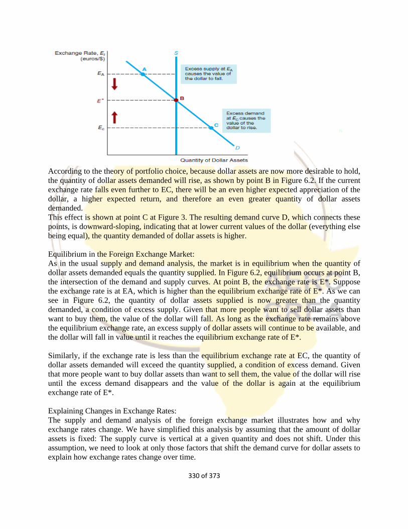
330 of 373

According to the theory of portfolio choice, because dollar assets are now more desirable to hold,

the quantity of dollar assets demanded will rise, as shown by point B in Figure 6.2. If the current

exchange rate falls even further to EC, there will be an even higher expected appreciation of the

dollar, a higher expected return, and therefore an even greater quantity of dollar assets

demanded.

This effect is shown at point C at Figure 3. The resulting demand curve D, which connects these

points, is downward-sloping, indicating that at lower current values of the dollar (everything else

being equal), the quantity demanded of dollar assets is higher.

Equilibrium in the Foreign Exchange Market:

As in the usual supply and demand analysis, the market is in equilibrium when the quantity of

dollar assets demanded equals the quantity supplied. In Figure 6.2, equilibrium occurs at point B,

the intersection of the demand and supply curves. At point B, the exchange rate is E*. Suppose

the exchange rate is at EA, which is higher than the equilibrium exchange rate of E*. As we can

see in Figure 6.2, the quantity of dollar assets supplied is now greater than the quantity

demanded, a condition of excess supply. Given that more people want to sell dollar assets than

want to buy them, the value of the dollar will fall. As long as the exchange rate remains above

the equilibrium exchange rate, an excess supply of dollar assets will continue to be available, and

the dollar will fall in value until it reaches the equilibrium exchange rate of E*.

Similarly, if the exchange rate is less than the equilibrium exchange rate at EC, the quantity of

dollar assets demanded will exceed the quantity supplied, a condition of excess demand. Given

that more people want to buy dollar assets than want to sell them, the value of the dollar will rise

until the excess demand disappears and the value of the dollar is again at the equilibrium

exchange rate of E*.

Explaining Changes in Exchange Rates:

The supply and demand analysis of the foreign exchange market illustrates how and why

exchange rates change. We have simplified this analysis by assuming that the amount of dollar

assets is fixed: The supply curve is vertical at a given quantity and does not shift. Under this

assumption, we need to look at only those factors that shift the demand curve for dollar assets to

explain how exchange rates change over time.

331 of 373

Shifts in the Demand for Domestic Assets:

As we have seen, the quantity of domestic (dollar) assets demanded depends on the relative

expected return on dollar assets. To see how the demand curve shifts, we need to determine how

the quantity demanded changes, holding the current exchange rate, Et, constant, when other

factors change. For insight into the direction in which the demand curve will shift, suppose you

are an investor who is considering putting funds into domestic (dollar) assets. When a factor

changes, you must decide whether, at a given level of the current exchange rate and holding all

other variables constant, you would earn a higher or lower expected return on dollar assets versus

foreign assets. This decision will tell you whether you want to hold more or fewer dollar assets

and thus whether the quantity demanded will increase or decrease at each level of the exchange

rate. The direction of the change in the quantity demanded at each exchange rate indicates which

way the demand curve will shift. In other words, if the relative expected return on dollar assets

rises, holding the current exchange rate constant, the demand curve will shift to the right. If the

relative expected return falls, the demand curve will shift to the left.

Domestic Interest Rate, iD Suppose that dollar assets pay an interest rate of iD. When the

domestic interest rate on dollar assets iD rises, holding the current exchange rate Et and

everything else constant, the return on dollar assets increases relative to the return on foreign

assets, and so people will want to hold more dollar assets. The quantity of dollar assets

demanded increases at every value of the exchange rate, as shown by the rightward shift of the

demand curve from D1 to D2 in Figure 6.3. The new equilibrium is reached at point 2, the

intersection of D2 and S, and the equilibrium exchange rate rises from E1 to E2. An increase in

the domestic interest rate iD shifts

the demand curve for domestic assets D to the right and causes the domestic currency

to appreciate (Ec ).

Conversely, if iD falls, the relative expected return on dollar assets falls, the demand curve shifts

to the left, and the exchange rate falls. A decrease in the domestic interest rate iD shifts the

demand curve for domestic assets D to the left and causes the domestic currency to depreciate

(ET).

Foreign Interest Rate, iF Suppose foreign assets pay an interest rate of iF. When the foreign

interest rate iF rises, holding the current exchange rate and everything else constant, the return on

foreign assets rises relative to the return on dollar assets. Thus the relative expected return on

dollar assets falls. Now people want to hold fewer dollar assets, and the quantity demanded

decreases at every value of the exchange rate. This scenario is shown by the leftward shift of the

demand curve from D1 to D2. The new equilibrium is reached at point 2, when the value of the

dollar has fallen. Conversely, a decrease in iF raises the relative expected return on dollar assets,

shifts the demand curve to the right, and raises the exchange rate. To summarize, an increase in

the foreign interest rate iF shifts the demand curve D to the left and causes the domestic currency

to depreciate; a fall in the foreign interest rate iF shifts the demand curve D to the right and

causes the domestic currency to appreciate.

Changes in the Expected Future Exchange Rate, Eet+1 Expectations about the future value of the

exchange rate play an important role in shifting the current demand curve because the demand

332 of 373

for domestic assets, like that for any physical or financial asset, depends on the future resale

price. Given the current exchange rate Et, any factor that causes the expected future exchange

rate Eet+1 to rise increases the expected appreciation of the dollar. The result is a higher relative

expected return on dollar assets, which increases the demand for dollar assets at every exchange

rate, thereby shifting the demand curve to the right from D1 to D2 in Figure 6. The equilibrium

exchange rate rises to point 2 at the intersection of the D2 and S curves. A rise in the expected

future exchange rate Eet+1 shifts the demand curve to the right and causes an appreciation of the

domestic currency. According to the same reasoning, a fall in the expected future exchange rate

Eet+1 shifts the demand curve to the left and causes a depreciation of the currency.

Comparing Expected Returns on Domestic and Foreign Assets

As we have done so far, let’s treat the United States as the home country, so domestic assets are

denominated in dollars. For simplicity, we use euros to stand for any foreign country’s currency,

so foreign assets are denominated in euros. Suppose that dollar assets pay an interest rate of iD

and do not have any possible capital gains, so that they have an expected return payable in

dollars of iD. Similarly, suppose that foreign assets have an interest rate of iF and an expected

return payable in the foreign currency, euros, of iF. To compare the expected returns on dollar

assets and foreign assets, investors must convert the returns into the currency unit that they use.

First, let us examine how François the Foreigner compares the returns on dollar assets and

foreign assets denominated in his currency, the euro. When he considers the expected return on

dollar assets in terms of euros, he recognizes that it does not equal iD; instead, the expected

return must be adjusted for any expected appreciation or depreciation of the dollar. If François

expects the dollar to appreciate by 3%, for example, the expected return on dollar assets in terms

of euros would be 3% higher than iD because the dollar is expected to become worth 3% more in

terms of euros.

Thus, if the interest rate on dollar assets is 4%, with an expected 3% appreciation of the dollar,

the expected return on dollar assets in terms of euros is 7%: the 4% interest rate plus the 3%

expected appreciation of the dollar. Conversely, if the dollar is expected to depreciate by 3%

over the year, the expected return on dollar assets in terms of euros will be only 1%: the 4%

interest rate minus the 3% expected depreciation of the dollar.

Writing the current exchange rate (the spot exchange rate) as Et and the expected

exchange rate for the next period as 𝐸𝑡+1

𝑒 −𝐸𝑡

𝐸𝑡 Our reasoning indicates that the expected return on

dollar assets RD in terms of foreign currency can be written as the sum of the interest rate on

dollar

assets plus the expected appreciation of the dollar.

𝑅𝐷𝑖𝑛 𝑡𝑒𝑟𝑚𝑠 𝑜𝑓 𝑒𝑢𝑟𝑜𝑠 = 𝑖𝐷 +𝐸𝑡+1

𝑒 − 𝐸𝑡

𝐸𝑡

However, François’s expected return on foreign assets RF in terms of euros is just

iF. Thus, in terms of euros, the relative expected return on dollar assets (that is, the difference

333 of 373

between the expected returns on dollar assets and euro assets) is calculated by

subtracting iF from the expression above to yield

𝑅𝐷𝑖𝑛 𝑡𝑒𝑟𝑚𝑠 𝑜𝑓 𝑑𝑜𝑙𝑙𝑎𝑟𝑠 = 𝑖𝑓 −𝐸𝑡+1

𝑒 −𝐸𝑡

𝐸𝑡 (1)

As the relative expected return on dollar assets increases, foreigners will want to hold

more dollar assets and fewer foreign assets.

Next let us look at the decision to hold dollar assets versus euro assets from Al the

American’s point of view. Following the same reasoning we used in François’s case, we

know that the expected return on foreign assets RF in terms of dollars is the interest

rate on foreign assets iF plus the expected appreciation of the foreign currency, which is

equal to minus the expected appreciation of the dollar,

𝑅𝑒𝑙𝑎𝑡𝑖𝑣𝑒𝑅𝐷 = 𝑖𝐷 − (𝑖𝑓 −𝐸𝑡+1

𝑒 − 𝐸𝑡

𝐸𝑡) = 𝑖𝐷 − 𝑖𝑓 +

𝐸𝑡+1𝑒 − 𝐸𝑡

𝐸𝑡

This equation is the same as Equation 1 describing François’s relative expected return on dollar

assets (calculated in terms of euros). The key point here is that the relative expected return on

dollar assets is the same whether it is calculated by François in terms of euros or by Al in terms

of dollars. Thus, as the relative expected return on dollar assets increases, both foreigners and

domestic residents respond in exactly the same way—both will want to hold more dollar assets

and fewer foreign assets.

Interest Parity Condition

We currently live in a world in which capital mobility exists: Foreigners can easily purchase

American assets, and Americans can easily purchase foreign assets. If few impediments to

capital mobility are present and we are looking at assets that have similar risk and liquidity—say,

foreign and American bank deposits—then it is reasonable to assume that the assets are perfect

substitutes (that is, equally desirable). When capital is mobile and assets are perfect substitutes, if

the expected return on dollar assets is greater than that on foreign assets, both foreigners and

Americans will want to hold only dollar assets and will be unwilling to hold foreign assets.

Conversely, if the expected return on foreign assets is higher than that on dollar assets, both

foreigners and Americans will not want to hold dollar assets and will want to hold only foreign

assets. Therefore, for existing supplies of both dollar assets and foreign assets to be held, it must

be the case that no difference exists in their expected returns; that is, the relative expected return

in Equation 1 must equal zero. This condition can be rewritten as

𝑖𝐷 = (𝑖𝑓 −𝐸𝑡+1

𝑒 −𝐸𝑡

𝐸𝑡) (2)

334 of 373

This equation, called the interest parity condition, states that the domestic interest rate equals the

foreign interest rate minus the expected appreciation of the domestic currency. Equivalently, this

condition can be stated in a more intuitive way: The domestic interest rate equals the foreign

interest rate plus the expected appreciation of the foreign currency. If the domestic interest rate is

higher than the foreign interest rate, there is a positive expected appreciation of the foreign

currency, which compensates for the lower foreign interest rate. A domestic interest rate of 5%

versus a foreign interest rate of 3% means that the expected appreciation of the foreign currency

must be 2% (or, equivalently, that the expected depreciation of the dollar must be 2%).

The interest parity condition can be looked at in several ways. First, recognize that interest parity

simply means that the expected returns are the same on both dollar assets and foreign assets. To

see this, note that the left side of the interest parity condition (Equation 2) is the expected return

on dollar assets, while the right side is the expected return on foreign assets, both calculated in

terms of a single currency, the U.S. dollar. Given our assumption that domestic and foreign

assets are perfect substitutes (equally desirable), the interest parity condition is an equilibrium

condition for the foreign exchange market. Only when the exchange rate is such that expected

returns on domestic and foreign assets are equal—that is, when interest parity holds—will

investors be willing to hold both domestic and foreign assets.

With some algebraic manipulation, we can rewrite the interest parity condition in

𝐸𝑡 = (𝐸𝑡+1

𝑒

𝑖𝑓 − 𝑖𝐷 + 1 )

This equation produces exactly the same results that we derived in the supply and\ demand

analysis given in the text: If iD rises, the value of the denominator decreases and so Et rises. If iF

rises, the value of the denominator increases and so Et falls. If 𝐸𝑡+1𝑒 rises, the value of the

numerator increases and so Et rises.

Effects of Changes in Interest Rates on the Equilibrium Exchange Rate

Our analysis has revealed the factors that affect the value of the equilibrium exchange rate. Now

we use this analysis to take a closer look at the response of the exchange rate to changes in

interest rates and money growth. Changes in domestic interest rates iD are often cited as a major

factor affecting exchange rates. For example, we see headlines in the financial press like this

one: “Dollar Recovers as Interest Rates Edge Upward.” But is the positive correlation suggested

in this headline true in every case?

Not necessarily, because to analyze the effects of interest rate changes, we must carefully

distinguish the sources of the changes. The Fisher equation states that a nominal interest rate

such as iD equals the real interest rate plus expected inflation: i = ir + _e. The Fisher equation

thus indicates that the interest rate iD can change for two reasons: Either the real interest rate ir

changes or the expected inflation rate πe changes. The effect on the exchange rate is quite

different, depending on which of these two factors is the source of the change in the nominal

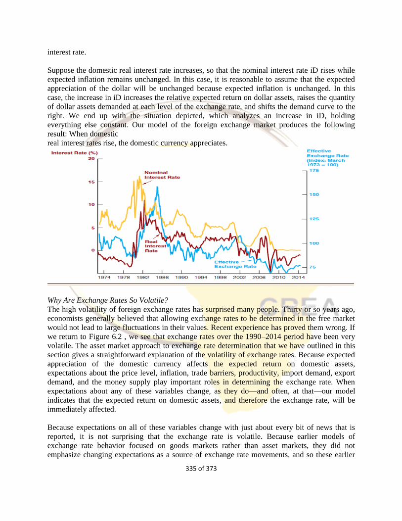
335 of 373

interest rate.

Suppose the domestic real interest rate increases, so that the nominal interest rate iD rises while

expected inflation remains unchanged. In this case, it is reasonable to assume that the expected

appreciation of the dollar will be unchanged because expected inflation is unchanged. In this

case, the increase in iD increases the relative expected return on dollar assets, raises the quantity

of dollar assets demanded at each level of the exchange rate, and shifts the demand curve to the

right. We end up with the situation depicted, which analyzes an increase in iD, holding

everything else constant. Our model of the foreign exchange market produces the following

result: When domestic

real interest rates rise, the domestic currency appreciates.

Why Are Exchange Rates So Volatile?

The high volatility of foreign exchange rates has surprised many people. Thirty or so years ago,

economists generally believed that allowing exchange rates to be determined in the free market

would not lead to large fluctuations in their values. Recent experience has proved them wrong. If

we return to Figure 6.2 , we see that exchange rates over the 1990–2014 period have been very

volatile. The asset market approach to exchange rate determination that we have outlined in this

section gives a straightforward explanation of the volatility of exchange rates. Because expected

appreciation of the domestic currency affects the expected return on domestic assets,

expectations about the price level, inflation, trade barriers, productivity, import demand, export

demand, and the money supply play important roles in determining the exchange rate. When

expectations about any of these variables change, as they do—and often, at that—our model

indicates that the expected return on domestic assets, and therefore the exchange rate, will be

immediately affected.

Because expectations on all of these variables change with just about every bit of news that is

reported, it is not surprising that the exchange rate is volatile. Because earlier models of

exchange rate behavior focused on goods markets rather than asset markets, they did not

emphasize changing expectations as a source of exchange rate movements, and so these earlier

336 of 373

models did not predict substantial fluctuations in exchange rates. The failure of earlier models to

explain volatility is one

reason why they are no longer so popular. The more modern approach developed here

emphasizes that the foreign exchange market is like any other asset market in which expectations

of the future matter. The foreign exchange market, like other asset markets such as the stock

market, displays substantial price volatility, and foreign exchange rates are notoriously hard to

forecast.

Balance of Payments Approaches

The balance of payments is a statistical record of all the economic transactions between residents

of the reporting country and residents of the rest of the world during a given time period. It

reveals how many goods and services the country has been exporting and importing and whether

the country has been borrowing from or lending to the rest of the world. In addition, whether or

not the central monetary authority (usually the central bank) has added to or reduced its reserves

of foreign currency is reported in the statistics.

Open Economy Identities

In an open economy, gross domestic product (GDP) differs from that of a closed economy

because there is an additional injection, export expenditure which represents foreign expenditure

on domestically produced goods. There is also an additional leakage expenditure on imports

which represents domestic expenditure on foreign goods and raises foreign national income.

The identity for an open economy is given by:

Y = 𝐶 + 𝐼 + 𝐺 + 𝑋 − 𝑀

If taxation is deducted;

𝑌𝑑 = 𝐶 + 𝐼 + 𝐺 + 𝑋 − 𝑀 − 𝑇

Given that private savings is S = 𝑌𝑑 - C

(X – M) = (S –I) + (T – G)

This implies that current account deficit depends on either private dissaving and/or a government

deficit. By re-arrangement;

I + G + X = S + T + M

Open economy multipliers

Keynesian analysis make assumptions about the determinants of the various components of

national income.

Government expenditure and exports are assumed to be exogenous- government expenditure is

determined independently by political decision, and exports by foreign expenditure decisions and

foreign income.

Domestic consumption is partly autonomous and partly determined by the level of national

income.

This is denoted algebraically by;

C = Ca + cY

Import expenditure is assumed to be partly autonomous and partly a positive function of the level

Current account

balance

Net savings/Dissavings

of the private sector

Government deficit/surplus

337 of 373

of domestic income,

M = Ma + mY

Y = Ca + cY + I + G + X - Ma - mY

(1 – c + m)Y = Ca + I + G + X - Ma

Given that (1 - c) is equal to the marginal propensity to save, s,

Y = 1

s+m(Ca + I + G + X - Ma) this can be transformed into difference form to yield;

Yd = 1

s+m(dCa + dI + dG + dX - dMa), where d in front of a variable represents the change in the

variable

Government expenditure multiplier

This shows the increase in national income resulting from a given increase in government expen-

diture. dy

dG =

1

s+m > 0

This implies that an increase in government expenditure will have an expansionary effect on

national income, the size of which depends upon the marginal propensity to save and the

marginal propensity to import

Export multiplier dy

dX =

1

s+m > 0

In practice, government expenditure tends to be somewhat more biased to domestic output than

private consumption expenditure. This implies that the value of m is smaller in the case of the

government expenditure multiplier than in the case of the export multiplier. Thus, an increase in

government expenditure will have a more expansionary effect on domestic output than an

equivalent increase in exports. The savings plus import expenditures (s + m) are assumed to

increase as income rises, reflected by the upward slope of the injections schedule. Because the

sum of the marginal propensity to import and save is less than unity this schedule has a slope less

than unity.

An increase in exports or government expenditure or Investment results in an upward shift of the

Injections schedule from (I+G+X)1 to (I+G+X)2 and this rise in income induces more saving

and import expenditure but overall the increase in income from Y1 to Y2 is greater than the initial

increase in injections. The lower the marginal propensities to save and import, the less steep the

leakages schedule and the greater the increase in income.

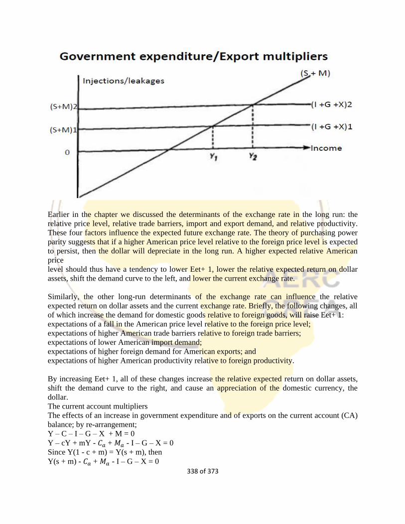
338 of 373

Earlier in the chapter we discussed the determinants of the exchange rate in the long run: the

relative price level, relative trade barriers, import and export demand, and relative productivity.

These four factors influence the expected future exchange rate. The theory of purchasing power

parity suggests that if a higher American price level relative to the foreign price level is expected

to persist, then the dollar will depreciate in the long run. A higher expected relative American

price

level should thus have a tendency to lower Eet+ 1, lower the relative expected return on dollar

assets, shift the demand curve to the left, and lower the current exchange rate.

Similarly, the other long-run determinants of the exchange rate can influence the relative

expected return on dollar assets and the current exchange rate. Briefly, the following changes, all

of which increase the demand for domestic goods relative to foreign goods, will raise Eet+ 1:

expectations of a fall in the American price level relative to the foreign price level;

expectations of higher American trade barriers relative to foreign trade barriers;

expectations of lower American import demand;

expectations of higher foreign demand for American exports; and

expectations of higher American productivity relative to foreign productivity.

By increasing Eet+ 1, all of these changes increase the relative expected return on dollar assets,

shift the demand curve to the right, and cause an appreciation of the domestic currency, the

dollar.

The current account multipliers

The effects of an increase in government expenditure and of exports on the current account (CA)

balance; by re-arrangement;

Y – C – I – G – X + M = 0

Y – cY + mY - 𝐶𝑎 + 𝑀𝑎 - I – G – X = 0

Since Y(1 - c + m) = Y(s + m), then

Y(s + m) - 𝐶𝑎 + 𝑀𝑎 - I – G – X = 0

339 of 373

mY - 𝑚

𝑠+𝑚 (𝐶𝑎 - 𝑀𝑎 + 𝐼 + 𝐺 + 𝑋) = 0

Adding Ma and X to each side, recalling that M = Ma + mY and rearranging yields;

CA = X - M = X - Ma - 𝑚

𝑠+𝑚 (𝐶𝑎 - 𝑀𝑎 + 𝐼 + 𝐺 + 𝑋) 𝑖𝑛 𝑑𝑖𝑓𝑓𝑒𝑟𝑒𝑛𝑐𝑒 𝑓𝑜𝑟𝑚;

dCA = dX - dMa - 𝑚

𝑠+𝑚 (𝑑𝐶𝑎 - 𝑑𝑀𝑎 + 𝑑𝐼 + 𝑑𝐺 + 𝑑𝑋)

the effects of an increase in government expenditure on the current account balance is given by; 𝑑𝐶𝐴

𝑑𝐺 = -

𝑚

𝑠+𝑚 < 0

Thus an increase in government spending leads to a deterioration of the current account balance

which is some fraction of the initial increase in government expenditure.

the effect of an increase in exports on the current balance; the multiplier is given by; 𝑑𝐶𝐴

𝑑𝑋 = 1 -

𝑚

𝑠+𝑚 =

𝑠+ 𝑚

𝑠+𝑚 -

𝑚

𝑠+𝑚=

𝑠

𝑠+𝑚 > 0

Since s/(s + m) is less than unity, an increase in exports leads to an improvement in the current

account balance that is less than the initial increase in exports.

This is because part of the Increase in income resulting from the additional exports is offset to

some extent by increase in expenditure on imports.

Elasticity Approach to Balance of Payments

Marshall-Lerner Condition

The elasticity approach investigates the relationship between the exchange rate and the balance

of payments (current account-trade balance). It assumes that if the BOP is in equilibrium,

devaluation can improve the balance of payments. However, for devaluation to function

successfully, the total of the price elasticity of domestic and foreign demand for imports has to

increase. When a country devalues a currency, it improves the balance of payments under ideal

conditions. This ideal condition is known as the Marshall-Lerner condition. The analysis was

pioneered by Alfred Marshall (1923) and Abba Lerner (1944), and later extended by Joan

Robinson (1937) and Fritz Machlup (1939).

Assumptions:

The supply elasticities for exports and imports are perfectly elastic, so that changes in demand

volumes have no effect on prices.

Domestic and foreign prices are fixed so that changes in relative prices are caused by changes in

the nominal exchange rate.

Income levels are fixed in the devaluing country.

The price elasticities of demand for exports and imports are arc elasticities.

Price elasticities refer to absolute values.

The country’s current account balance equals its trade balance.

Given these assumptions, when a country devalues its currency, the domestic prices of its

imports are raised and the foreign prices of its exports are reduced. Thus, devaluation helps to

improve BOP deficit of a country by increasing its exports and reducing its imports. But the

extent to which it will succeed depends on the country’s price elasticities of domestic demand for

imports and foreign demand for exports.

340 of 373

This is what the Marshall-Lerner condition states: when the sum of price elasticities of demand

for exports and imports in absolute terms is greater than unity, devaluation will improve the

country’s balance of payments

The current account balance when expressed in terms of the domestic currency is given by;

CA = 𝑃𝑋𝑣 - 𝑆𝑃∗𝑀𝑣

where P is the domestic price level, Xv is the volume of domestic exports, S is the exchange rate,

P* is the foreign price level and Mv is the volume of imports.

By simplification, the domestic and foreign price levels are set at unity; the value of domestic

exports (P Xv) is given by X; while the foreign currency value of imports (P* Mv) is given by

M. Using these simplifications;

CA = X – SM

In difference form;

dCA = dX – S dM – M dS, by dividing through by dS; 𝑑𝐶𝐴

𝑑𝑆 =

𝑑𝑋

𝑑𝑆 − 𝑆

𝑑𝑀

𝑑𝑆 - M

𝑑𝑆

𝑑𝑆

The price elasticity of demand for exports 𝜂𝑥 − the percentage change in exports over the

percentage change in price as represented by the percentage change in the exchange rate;

𝜂𝑥 = 𝑑𝑋/𝑋

𝑑𝑆/𝑆

dx = 𝜂𝑥 𝑑𝑆 𝑋

𝑆

The price elasticity of demand for imports 𝜂𝑚- the percentage change in imports over the

percentage change in their price as represented by the percentage change in the exchange rate;

𝜂𝑚 = - 𝑑𝑀/𝑀

𝑑𝑆/𝑆

dM = - 𝜂𝑚 𝑑𝑆 𝑀

𝑆

By substitution; 𝑑𝐶𝐴

𝑑𝑆 =

𝜂𝑥 𝑋

𝑆 + 𝜂𝑚 M – M by dividing by M

𝑑𝐶𝐴

𝑑𝑆 1

𝑀 =

𝜂𝑥 𝑋

𝑆 𝑀 + 𝜂𝑚 -1

Assuming a balanced trade, X/SM =1, then by re-arrangement. 𝑑𝐶𝐴

𝑑𝑆 = M(𝜂𝑥 + 𝜂𝑚 -1) – Marshal-Lerner condition

This implies that when the current account is in equilibrium, a devaluation will improve the

current account.

Thus, dCA/dS > 0 only if the sum of the foreign elasticity of demand for exports and the home

country elasticity of demand for imports is greater than unity. Thus, (𝜂𝑥 + 𝜂𝑚) > 1. If the sum of these two elasticities is less than unity, then a devaluation will lead to a

deterioration of the current account.

The J-Curve Effect

Empirical studies have established that in the short-run, the Marshall-Lerner condition does not

hold. This is based on the notion that elasticities are lower in the short run than in the long run, in

which case the Marshall-Lerner conditions may not hold in the short run but may hold in the

medium to long run. The effects of devaluation on domestic prices and demand for exports and

imports will take time for consumers and producers to adjust themselves to the new situation.

The idea underlying the J-curve effect is that in the short run export volumes and import volumes

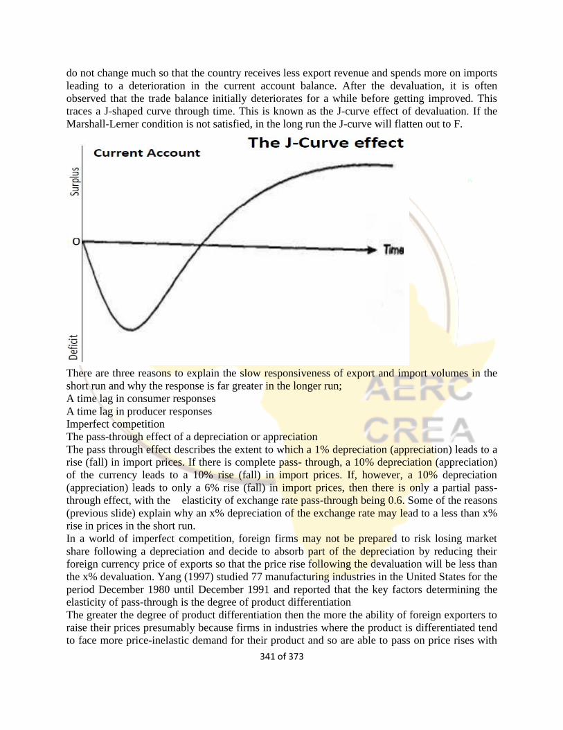
341 of 373

do not change much so that the country receives less export revenue and spends more on imports

leading to a deterioration in the current account balance. After the devaluation, it is often

observed that the trade balance initially deteriorates for a while before getting improved. This

traces a J-shaped curve through time. This is known as the J-curve effect of devaluation. If the

Marshall-Lerner condition is not satisfied, in the long run the J-curve will flatten out to F.

There are three reasons to explain the slow responsiveness of export and import volumes in the

short run and why the response is far greater in the longer run;

A time lag in consumer responses

A time lag in producer responses

Imperfect competition

The pass-through effect of a depreciation or appreciation

The pass through effect describes the extent to which a 1% depreciation (appreciation) leads to a

rise (fall) in import prices. If there is complete pass- through, a 10% depreciation (appreciation)

of the currency leads to a 10% rise (fall) in import prices. If, however, a 10% depreciation

(appreciation) leads to only a 6% rise (fall) in import prices, then there is only a partial pass-

through effect, with the elasticity of exchange rate pass-through being 0.6. Some of the reasons

(previous slide) explain why an x% depreciation of the exchange rate may lead to a less than x%

rise in prices in the short run.

In a world of imperfect competition, foreign firms may not be prepared to risk losing market

share following a depreciation and decide to absorb part of the depreciation by reducing their

foreign currency price of exports so that the price rise following the devaluation will be less than

the x% devaluation. Yang (1997) studied 77 manufacturing industries in the United States for the

period December 1980 until December 1991 and reported that the key factors determining the

elasticity of pass-through is the degree of product differentiation

The greater the degree of product differentiation then the more the ability of foreign exporters to

raise their prices presumably because firms in industries where the product is differentiated tend

to face more price-inelastic demand for their product and so are able to pass on price rises with

342 of 373

less fear of losing sales

Criticisms

Misleading: The elasticity approach which applies the Marshallian concept of elasticity to solve

BOP deficit is misleading. This is because it has relevance only to incremental change along a

demand or supply curve and to problems dealing with shifts in these curves. Moreover, it

assumes constant purchasing power of money which is not relevant to devaluation of the

country’s currency.

Partial Elasticities: The elasticity approach has been criticised because it uses partial elasticities

which exclude all factors except relative prices and quantities of exports and imports. This is

applicable only to single-commodity trade rather than to a multi-commodity trade. It makes this

approach unrealistic.

Supplies not Perfectly Elastic: The Marshall-Lerner condition assumes perfectly elastic supplies

of exports and imports. But this assumption is unrealistic because the country may not be in a

position to increase the supply of its exports when they become cheap with devaluation of its

currency.

Partial Equilibrium Analysis: The elasticity approach assumes domestic price and income levels

to be stable within the devaluing country. It, further, assumes that there are no restrictions in

using additional resources into production for exports. These assumptions show that this analysis

is based on the partial equilibrium analysis. It, therefore, ignores the feedback effects of a price

change in one product on incomes, and consequently on the demand for goods. This is a serious

defect of the elasticity approach because the effects of devaluation always spread to the entire

economy

Inflationary: Devaluation can lead to inflation in the economy. Even if it succeeds in improving

the balance of payments, it is likely to increase domestic incomes in export and import-

competing industries. But these increased incomes will affect the BOP directly by increasing the

demand for imports, and indirectly by increasing the overall demand and thus raising the prices

within the country.

Ignores Income Distribution: The elasticity approach ignores the effects of devaluation on

income distribution. Devaluation leads to the reallocation of resources. It takes away resources

from the sector producing non-traded goods to export and import-competing industries sector.

This will tend to increase the incomes of the factors of production employed in the latter sector

and reduce that of the former sector.

Applicable in the Long Run: As discussed above in the J-curve effect of devaluation, the

Marshall-Lerner condition is applicable in the long-run and not in the short. This is because it

takes time for consumers and producers to adjust themselves when there is devaluation of the

domestic currency.

Ignores Capital Flows: This approach is applicable to BOP on current account or balance of

trade. But BOP deficit of a country is mainly the result of the outflow of capital. It thus ignores

BOP on capital account. Devaluation as a remedy is meant to cut imports and the outflow of

capital and increase exports and the inflow of capital.

343 of 373

Absorption Approach to Balance of Payments

The absorption approach emphasizes changes in real domestic income as a determinant of a

nation’s balance of payments and exchange rate. This approach to balance of payments is also

known as the Keynesian approach because it is based on the Keynesian national income

relationships. It runs through the income effect of devaluation as against the price effect to the

elasticity approach.

The theory states that if a country has a deficit in its balance of payments, it means that people

are ‘absorbing’ more than they produce. Domestic expenditure on consumption and investment

is greater than national income. If they have a surplus in the balance of payments, they are

absorbing less. Expenditure on consumption and investment is less than national income. A

nation’s expenditures fall into four categories, consumption (c), investment (i), government (g),

and imports (m).

The total of these four categories is referred to as domestic absorption (a)

A C + I + G + M,

A nation’s real income (y) is equivalent to total expenditures on its output

Y C + I + G + X,

the current account (ca) is equivalent to ca x - m.

The absorption approach hypothesizes that a nation’s current account balance is determined by

the difference between real income and absorption, which can be written as:

Y - A = (C+I+G+X) - (C+I+G+M) = X - M,

OR Y - A = CA.

Here the BOP is defined as the difference between national income and domestic expenditure.

This approach was developed by Sydney Alexander in 1952.

Taking the equation for national income

Y = C + I + G + X – M and defining domestic absorption as;

A = C + I + G, the equation can be rearranged as follows;

CA = X-M = Y-A

This implies that the current balance represents the difference between domestic output and

domestic absorption.

By taking the difference;

dCA = dY – dA

This equation implies that the effects of a devaluation on the current account balance will depend

upon how it affects national income relative to how it affects domestic absorption.

Absorption can be divided up into two parts:

a rise in income will lead to an increase in absorption which is determined by the marginal

propensity to absorb, a,

a 'direct effect' on absorption which is all the other effects on absorption resulting from

devaluation denoted by 𝐴𝑑.

Thus, the change in total absorption dA, is given by;

dA = adY + d𝐴𝑑. by substitution.

dCA = (1-a)dY - d𝐴𝑑.

This reveals that a devaluation can affect the current account balance only by changing the

marginal propensity to absorb a, changing the level of income, dY, and by affecting direct

absorption, dAd. The condition for a devaluation to improve the current account is (1 - a)dY >

d𝐴𝑑. that is, any change in income not spent on absorption must exceed any change in direct

344 of 373

absorption

The effects of a devaluation on national income

If the marginal propensity to absorb is less than unity then a rise in income will raise the income

to absorption ratio and so improve the current account. Whereas, if income were to fall this

would raise the absorption to income ratio (as absorption would fall by less than income) which

would worsen the current account

Employment effect. If the economy is at less than full employment, then providing the Marshall-

Lerner condition is fulfilled there will be an increase in net exports following a devaluation

which will lead to an increase in national income via the foreign trade multiplier.

Terms of trade effect. A devaluation tends to make imports more expensive in domestic currency

terms which is not matched by a corresponding rise in export prices; this means that the terms of

trade deteriorate. The terms of trade effect lowers national income

The effects of a devaluation on direct absorption

If the devaluing country has idle resources, devaluation will increase exports and decrease

imports, income will rise and so will absorption. If the increase in absorption is less than the rise

in income, BOP will improve. So an improvement in BOP can be brought about by reduction in

direct absorption. Domestic absorption can fall automatically as a result of devaluation due to

real cash balance effect, money illusion and income redistribution

If a devaluation raises domestic income relative to domestic spending, current account improves.

If, however, devaluation raises domestic absorption relative to domestic income, the current

account deteriorates.

Real Cash Balance Effect:

When a country devalues its currency, its domestic prices rise. If the money supply remains

constant, the real value of cash balances held by the people falls and this reduce their expenditure

or absorption. If people hold assets and devaluation reduces their real cash balances, they sell

them. This reduces the prices of assets and increases interest rate. This, in turn, reduces

investment and consumption, absorption will be reduced. This is the asset effect of real cash

balance effect of devaluation.

Income Re-distribution Effect:

The rise in the general price index resulting from a devaluation is likely to have a number of

effects on the income distribution. If it redistributes income from those with a low marginal

propensity to absorb to those with a high marginal propensity to absorb it will increase direct

absorption.

Note that the rise in the general price index will tend to reduce the real income of those with

fixed incomes, but if overall income is unchanged then those with variable incomes would have

gained. Those with fixed incomes tend to have a high propensity to absorb, while those on

variable incomes are better off and have a lower propensity to absorb. If income is redistributed

from those with fixed incomes to those with variable incomes, then this income redistribution

effect will tend to reduce direct absorption.

A devaluation often leads to an improvement of company profits through increased sales in

export and import-competing industries. Real wages are reduced by the rise in the aggregate

price index and take time to catch up. The effect on direct absorption of this redistribution is not

clear, while firms may have a lower tendency to absorb than workers this will be very much

dependent on their expectations about the future. If these expectations are very favourable then

345 of 373

the devaluation and profits rise may stimulate investment and even raise direct absorption.

There may be considerable income adjustments within groups of companies and workers. Some

companies' profits will benefit from a devaluation as export sales rise, however, some firms that

are reliant on imported inputs may find that the costs increases reduce their profit margins.

Similarly, some workers will be able to protect themselves against the induced price rise because

they are represented by strong trade unions, while others with no union representation may not

secure compensating rises. The overall effect on direct absorption will then depend on whether

the companies and workers that gain have a higher propensity to absorb than those that lose

Money Illusion Effect:

When prices rise because of devaluation, consumers may suffer money illusion and buy exactly

the same bundle of goods as before, even though their real spending power has been reduced. If

this is the case they are actually spending more on direct absorption than before. However, the

money illusion effect may work in reverse and consumers, because of the price rises, may

actually decide to cut back direct absorption in more than proportion to the price rise so that

direct absorption falls. Whatever way the money illusion effect works it is unlikely to be very

significant and is most probably only a temporary rather than a permanent factor

1.6.2 Money and BOP Adjustment

Monetary Approach to Balance of Payments

The monetary view of the balance of payments or the global monetarist approach immerged late

1950s. The monetary approach emerged in 1950s first as a monetary approach to the balance of

payment and then was refocused to the exchange rates[14]. The first champion of the monetary

approach, later redefined by Hahn[16], Pearce[17], Prais[18], Mundell[19,20], Johnson, and

other followers. These monetarists suggest that the balance of payment is a monetary

phenomenon. Thus, since the exchange rate is the price of one currency expressed in terms of

another currency, the balance of payment should be expressed from the point of view of supply

and demand of money.

The model starts with the reasonable statement that, as the exchange rate is the relative price of

foreign and domestic money, it should be determined by the relative supply and demand for

these moneys. This simply suggests, if people demand more money than is being supplied by the

central bank then the excess demand for money would be met by inflow of money from abroad,

hence the trade balance will improve. On the contrary, if the central bank supplies more money

than is demanded, the excess supply of money is eliminated by outflow of money to the other

countries and this will worsen the trade balance. It is inherent therefore that, any excess demand

for goods, services and assets, resulting in a deficit of the balance of payments, reflects an excess

supply or demand of the stock of money. It seems the central point of the monetary approach to

the balance of payment is that balance of payment deficits or surpluses reflect stock

disequilibrium between demand and supply in the market for money.

With monetary approach therefore, it is important to emphasize the role of demand and supply of

money in determining the exchange rates. Thus, similar to any merchandise which is for sale, the

foreign exchange value is subjected to the law of supply and demand. This is the reason why the

exchange rate will be explained using the same geometric artifices which are used to explain the

formation of prices in general. Therefore, according to this approach, the exchange rate between

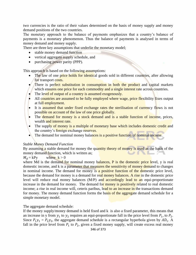
346 of 373

two currencies is the ratio of their values determined on the basis of money supply and money

demand positions of the two countries.

The monetary approach to the balance of payments emphasizes that a country’s balance of

payments is a monetary phenomenon. Thus the balance of payments is analysed in terms of

money demand and money supply.

There are three key assumptions that underlie the monetary model;

• stable money demand function

• vertical aggregate supply schedule, and

• purchasing power parity (PPP).

This approach is based on the following assumptions:

• The law of one price holds for identical goods sold in different countries, after allowing

for transport costs.

• There is perfect substitution in consumption in both the product and capital markets

which ensures one price for each commodity and a single interest rate across countries.

• The level of output of a country is assumed exogenously.

• All countries are assumed to be fully employed where wage, price flexibility fixes output

at full employment.

• It is assumed that under fixed exchange rates the sterilisation of currency flows is not

possible on account of the law of one price globally.

• The demand for money is a stock demand and is a stable function of income, prices,

wealth and interest rate.

• The supply of money is a multiple of monetary base which includes domestic credit and

the country’s foreign exchange reserves.

• The demand for nominal money balances is a positive function of nominal income.

Stable Money Demand Function

By assuming a stable demand for money the quantity theory of money is used as the basis of the

money demand function, which is written as;

𝑀𝑑 = kPy where k > 0

where Md is the demand for nominal money balances, P is the domestic price level, y is real

domestic income, and k is a parameter that measures the sensitivity of money demand to changes

in nominal income. The demand for money is a positive function of the domestic price level,

because the demand for money is a demand for real money balances. A rise in the domestic price

level will reduce real money balances (M/P) and accordingly lead to an equi-proportionate

increase in the demand for money. The demand for money is positively related to real domestic

income; a rise in real income will, ceteris paribus, lead to an increase in the transactions demand

for money. The money demand function forms the basis of the aggregate demand schedule for a

simple monetary model.

The aggregate demand schedule:

If the money supply/money demand is held fixed and k is also a fixed parameter, this means that

an increase in y from 𝑦1 to 𝑦2 requires an equi-proportionate fall in the price level from 𝑃1, to 𝑃2.

Since 𝑃1𝑦1 = 𝑃2𝑦2, the aggregate demand schedule is a rectangular hyperbola given by 𝐴𝐷1. A

fall in the price level from 𝑃1 to 𝑃2, given a fixed money supply, will create excess real money

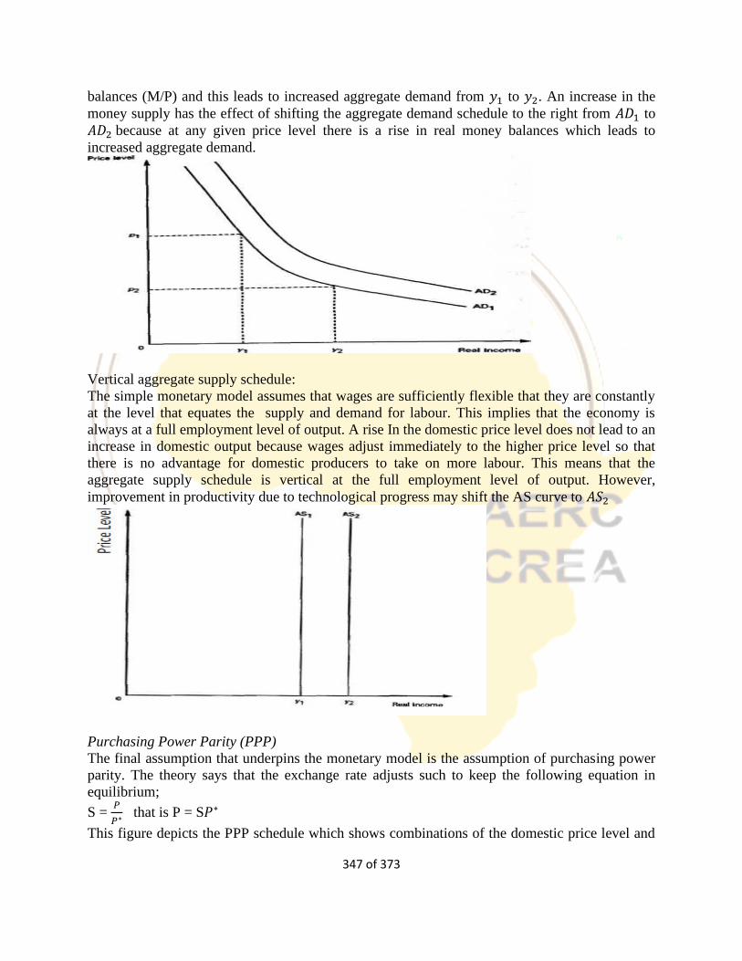
347 of 373

balances (M/P) and this leads to increased aggregate demand from 𝑦1 to 𝑦2. An increase in the

money supply has the effect of shifting the aggregate demand schedule to the right from 𝐴𝐷1 to

𝐴𝐷2 because at any given price level there is a rise in real money balances which leads to

increased aggregate demand.

Vertical aggregate supply schedule:

The simple monetary model assumes that wages are sufficiently flexible that they are constantly

at the level that equates the supply and demand for labour. This implies that the economy is

always at a full employment level of output. A rise In the domestic price level does not lead to an

increase in domestic output because wages adjust immediately to the higher price level so that

there is no advantage for domestic producers to take on more labour. This means that the

aggregate supply schedule is vertical at the full employment level of output. However,

improvement in productivity due to technological progress may shift the AS curve to 𝐴𝑆2

Purchasing Power Parity (PPP)

The final assumption that underpins the monetary model is the assumption of purchasing power

parity. The theory says that the exchange rate adjusts such to keep the following equation in

equilibrium;

S = 𝑃

𝑃∗ that is P = S𝑃∗

This figure depicts the PPP schedule which shows combinations of the domestic price level and

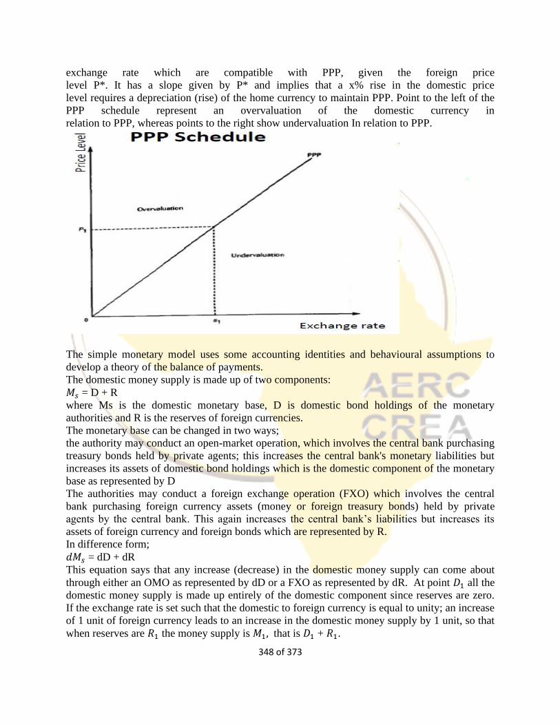
348 of 373

exchange rate which are compatible with PPP, given the foreign price

level P*. It has a slope given by P* and implies that a x% rise in the domestic price

level requires a depreciation (rise) of the home currency to maintain PPP. Point to the left of the

PPP schedule represent an overvaluation of the domestic currency in

relation to PPP, whereas points to the right show undervaluation In relation to PPP.

The simple monetary model uses some accounting identities and behavioural assumptions to

develop a theory of the balance of payments.

The domestic money supply is made up of two components:

𝑀𝑠 = D + R

where Ms is the domestic monetary base, D is domestic bond holdings of the monetary

authorities and R is the reserves of foreign currencies.

The monetary base can be changed in two ways;

the authority may conduct an open-market operation, which involves the central bank purchasing

treasury bonds held by private agents; this increases the central bank's monetary liabilities but

increases its assets of domestic bond holdings which is the domestic component of the monetary

base as represented by D

The authorities may conduct a foreign exchange operation (FXO) which involves the central

bank purchasing foreign currency assets (money or foreign treasury bonds) held by private

agents by the central bank. This again increases the central bank’s liabilities but increases its

assets of foreign currency and foreign bonds which are represented by R.

In difference form;

𝑑𝑀𝑠 = dD + dR

This equation says that any increase (decrease) in the domestic money supply can come about

through either an OMO as represented by dD or a FXO as represented by dR. At point 𝐷1 all the

domestic money supply is made up entirely of the domestic component since reserves are zero.

If the exchange rate is set such that the domestic to foreign currency is equal to unity; an increase

of 1 unit of foreign currency leads to an increase in the domestic money supply by 1 unit, so that

when reserves are 𝑅1 the money supply is 𝑀1, that is 𝐷1 + 𝑅1.

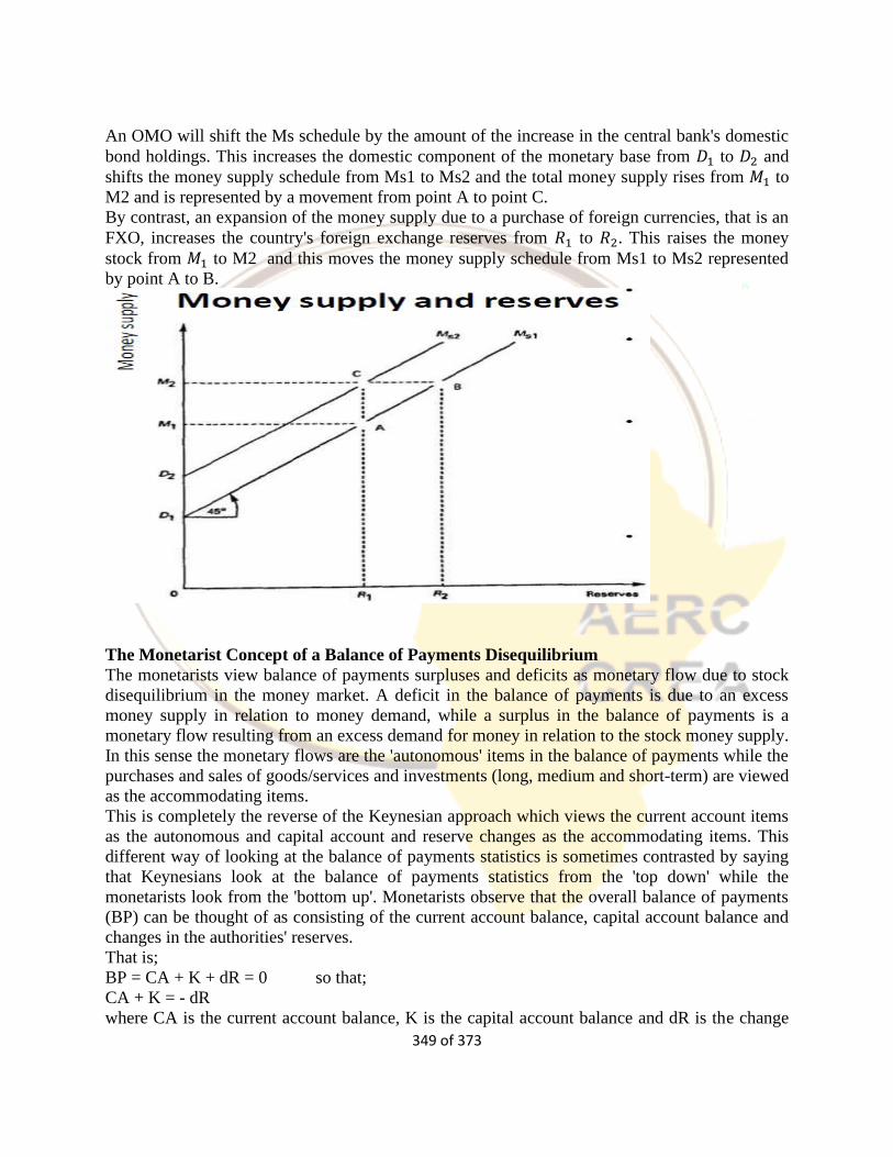
349 of 373

An OMO will shift the Ms schedule by the amount of the increase in the central bank's domestic

bond holdings. This increases the domestic component of the monetary base from 𝐷1 to 𝐷2 and

shifts the money supply schedule from Ms1 to Ms2 and the total money supply rises from 𝑀1 to

M2 and is represented by a movement from point A to point C.

By contrast, an expansion of the money supply due to a purchase of foreign currencies, that is an

FXO, increases the country's foreign exchange reserves from 𝑅1 to 𝑅2. This raises the money

stock from 𝑀1 to M2 and this moves the money supply schedule from Ms1 to Ms2 represented

by point A to B.

The Monetarist Concept of a Balance of Payments Disequilibrium

The monetarists view balance of payments surpluses and deficits as monetary flow due to stock

disequilibrium in the money market. A deficit in the balance of payments is due to an excess

money supply in relation to money demand, while a surplus in the balance of payments is a

monetary flow resulting from an excess demand for money in relation to the stock money supply.

In this sense the monetary flows are the 'autonomous' items in the balance of payments while the

purchases and sales of goods/services and investments (long, medium and short-term) are viewed

as the accommodating items.

This is completely the reverse of the Keynesian approach which views the current account items

as the autonomous and capital account and reserve changes as the accommodating items. This

different way of looking at the balance of payments statistics is sometimes contrasted by saying

that Keynesians look at the balance of payments statistics from the 'top down' while the

monetarists look from the 'bottom up'. Monetarists observe that the overall balance of payments

(BP) can be thought of as consisting of the current account balance, capital account balance and

changes in the authorities' reserves.

That is;

BP = CA + K + dR = 0 so that;

CA + K = - dR

where CA is the current account balance, K is the capital account balance and dR is the change

350 of 373

in the authorities reserves.

CA + K = - dR

According this equation, increases in reserves due to purchases of foreign currencies constitute a

surplus in the balance of payments, while falls in reserves resulting from purchases of the

domestic currency represent a deficit in the balance of payments. If the currency is left to float,

then reserves do not change and as far as the monetary view of the balance of payments is

concerned the balance of payments is in equilibrium. Under a floating exchange rate regime, a

current account deficit must be financed by an equivalent capital inflow so that the balance of

payments is in equilibrium.

The model is in equilibrium when aggregate demand is equal to aggregate supply at 𝑃1 𝑎𝑛𝑑 𝑌1. Also, PPP holds in the foreign exchange market at price level 𝑃1 and the exogenous foreign price

level P* the exchange rate compatible with PPP is given by 𝑆1. Finally, the money market is in

equilibrium, so with the money supply 𝑀1 made up of the domestic component Dl and reserve

component 𝑅1 is equal to money demand. The precise position of the money demand schedule is

determined by the domestic price level and domestic income level. Equilibrium in the money

market also implies equilibrium in the balance of payments.

Formal determination

In what follows, we will systematically go through the formal model of the Monetary Approach

to the Balance of Payments.

The monetary approach to the balance of payments argues that the BOP is mainly a monetary

phenomenon. This approach requires us to consider a country’s supply of and demand for

money. The money supply (Ms) can be seen either in terms of central bank liabilities:

Ms = a(BR + C), where

BR = reserves of commercial banks

C = currency held by nonbank public

a = the money multiplier

Or central bank assets

Ms = a(DR + IR), where

DR = domestic reserves

IR = international reserves

The money multiplier refers to the notion of multiple deposit creation. If the reserve requirement

is 10%, a new deposit of $1,000 creates $900 of excess reserves, which can be lent out. The loan

recipient deposits the $900 in her bank; this creates $810 of excess reserves which can be lent,

etc. The money multiplier is 1/r or 10. Anything that increases the assets of the central bank (or

equivalently, its liabilities) allows the money supply to expand via the multiplier process.

Suppose the central bank buys government securities or foreign exchange – in either case the

money supply is expanded. Money demand (L) is a function of several variables:

L = f[Y, P, i, W, E(p), O], where

Y = level of real income in economy

P = price level

i = interest rate

W = level of real wealth

E(p) = expected % Δ in price level

O = other variables that may affect L the Demand for Money

351 of 373

L is a positive function of Y, due to the transactions demand for money.

L is a positive function of P, since more cash is needed to make purchases when P rises.

L is a negative function of I; i is the opportunity cost of holding money.

L is a positive function of W; as a person’s wealth rises she will want to hold more money.

L is a negative function of E(p); if a person expects inflation he will hold less money.

Frequently a general expression for money demand is used:

L = kPY, where

P and Y are as discussed, and k is a constant embodying all other influences on money demand.

Money market equilibrium occurs when

Ms = L or

a(DR+IR) = a(BR+C) = f[Y,P,I,W,E(p),O]

or

Ms = kPY.

How can we understand balance of payments adjustments using money supply and demand? Let

us assume a fixed exchange rate system. What happens when the central bank increases Ms,

perhaps by purchasing government securities (increasing DR)?

BR and/or C will increase, and there will now be an excess supply of money.Current account

excess cash balances imply individuals spend more, bidding up P. Y and W may rise.Higher P

and Y will lead to lower exports (X) and higher imports (M).

Therefore, the excess supply of money leads to a current account deficit.

Private capital account:excess cash causes individual to bid up price of financial assets; this

drives down i. In the end, this causes a deficit in the private capital account. Together, these

effects indicate that a money supply increase leads to a balance of payments deficit.

To summarize:

Increase in Ms causes individuals to shift to non-money assets, including foreign goods and

assets.

This creates a BOP deficit.

When exchange rates are fixed, an increase in Ms leads to a BOP deficit. If the exchange rate is

not fixed, BOP deficits and surpluses will be eliminated by exchange rate adjustments.

Let’s look at exchange rate changes in terms of money demand and supply

What happens if Ms is increased? If Ms is increased; Individuals wish to purchase non-money

assets, including foreign goods and assets. This creates an “incipient” BOP deficit. The home

country’s currency will depreciate to eliminate the BOP deficit. If Ms is decreased then

Individuals wish to sell non-money assets, including foreign goods and assets. This creates an

“incipient” BOP surplus. The home country’s currency will appreciate to eliminate the BOP

surplus. If we assume that absolute purchasing power parity holds, then

e = PA/PB

Similarly, for Country B,

MsB = kBPBYB

It must be true that

𝑀𝑠𝐴

𝑀𝑠𝐵=

𝑘𝐴𝑃𝐴𝑌𝐴

𝑘𝐵𝑃𝐵𝑌𝐵

352 of 373

For Country A, monetary equilibrium means that

MsA = kAPAYA

This means that

𝑀𝑠𝐴

𝑀𝑠𝐵=

𝑘𝐴𝑌𝐴

𝑘𝐵𝑌𝐵𝑒

Rearranging yields

𝑒 =𝑘𝐵𝑌𝐵𝑀𝑠𝐴

𝑘𝐴𝑌𝐴𝑀𝑠𝐵

This expression demonstrates that an increase in Ms by Country A will lead to a depreciation of

the currency. Inflationary monetary policy only causes currency depreciation.

Monetary Policy Coordination: MsA and MsB

Portfolio Balance Approach to the BOP and the Exchange Rate

The approach extends the monetary approach to include other financial assets besides money. In

a two country model there will continue to be demand for money by each country’s citizens.

Now there will also be demand for home-country bonds (Bd) and for foreign bonds (Bf). Bd

yields interest return of id; Bf yields a return of if. The relationship between interest rates is as

follows:

id = if + xa – RP, where

RP is the risk premium associated with the imperfect international mobility of capital

xa is the expected percentage appreciation of the foreign currency, or [E(e)/e] – 1

Demand by home country individual for home money

L = f(id, if, xa, Yd, Pd, Wd), where

id = return on home-country bonds

if = return on foreign-country bonds

xa = expected appreciation of foreign currency

Yd = home country real income

Pd = home country price level

Wd = home country real wealth

Home money demand (L) will be:

inversely related to id.

Inversely related to if.

Inversely related to xa.

Positively related to Yd.

Positively related to Pd.

Positively related to Wd.

Demand by home country individual for home bonds

Bd = h(id, if, xa, Yd, Pd, Wd), where

Home bond demand will be

353 of 373

Positively related to id

Inversely related to if

Inversely related to xa

Inversely related to Yd

Inversely related to Pd

Positively related to Wd

Demand by home country individual for foreign bonds (multiplied by e so that it’s in terms of

domestic currency

eBf = j(id, if, xa, Yd, Pd, Wd), where

Foreign bond demand will be

Inversely related to id

Positively related to if

Positively related to xa

Inversely related to Yd

Inversely related to Pd

Positively related to Wd

Home country central bank sells government securities (i.e., decreases Ms and increase home

bond supply). id should rise, resulting in:

• decrease in home-country money demand,

• decrease in foreign bond demand, and

• increase in home bond demand.

Foreign investors switch towards holding home-country currency. Home country central bank

sells government securities (i.e., decreases Ms and increase home bond supply).

if should falls rise.

The foreign currency depreciates (e falls), assuming flexible exchange rates.

xa rises.

There are therefore second-round effects, continuing until a new portfolio balance is attained.

Home country individual believe home inflation is likely in the future.

Assume flexible exchange rates, xa should rise (that is, home citizens will expect a depreciation

of the home currency), resulting in:

• decrease in home-country money demand,

• decrease in home bond demand, and

• increase in foreign bond demand.

The home country currency depreciates. So, the expectation of a depreciation leads to a

depreciation. An increase in home country real income, leading to:

• increase in home-country money demand.

• decrease in home bond demand.

• decrease in foreign bond demand.

The home country currency appreciates under a flexible exchange rate system; a BOP surplus

occurs under a fixed exchange rate regime. An increase in home country bond supply causes

increase in id, which causes a capital inflow and an appreciation of the home country currency. It

also leads to increase in wealth, which (among other things) causes an increased demand for

foreign bonds and an depreciation of the home currency. On net, it is likely that the home

354 of 373

currency appreciates.

An increase in home country wealth because of home-country current account surplus leads to

an increase in money demand, leading to an increase in id. This also leads to an increase in

demand for foreign bonds and for domestic bonds, both of which lead to a decrease in id. On net,

it is not clear what will happen to the exchange rate.

An increase in supply of foreign bonds because of foreign government budget deficit, causes an

increase in the risk premium, and an appreciation of the home country currency.

Exchange Rate Overshooting

Exchange rate overshooting occurs when, in moving from one equilibrium to another, the

exchange rate goes beyond the new equilibrium before eventually returning to it.

Assume:

Country is small.

Perfect capital mobility exists.

Essentially, uncovered interest parity applies.

The relationship between the price level (P) and the exchange rate (e) should be negative because

a higher price increases demand for money, so id will rise. The result is an appreciation. If from

point B prices were to rise to P2, demand for money would rise, and the home currency would

appreciate (i.e., e falls). the Asset Market

Money and BOP adjustment

According to David Hume balance of payment moves towards equilibrium automatically as

national price levels adjust. With reference to the gold standard:

each nation’s money supply consisted of gold or paper money backed by gold each nation set

price of gold in terms of its currency free import and export of gold balance of payments surplus

causes nation to acquire gold and increase its money supply assuming balance of payments

deficit gold outflow (under classical gold standard) decrease money supply reduce domestic

price level and increase international competitiveness. This leads to an increase in exports and

decrease imports return to balance of payment equilibrium. Assuming a balance of payments

surplus, the business sector’s receipts from foreigners exceed payments. The domestic

commercial banks and the central bank accumulate reserves. When the commercial banks

deposit the foreign currency at the central bank, their reserves increase by the amount of the

surplus. This represents an increase in un-borrowed reserves and all other things being equal

expands the money supply by;

∆𝑀 = 𝐵

ℎ + 𝑧(1 − ℎ)

Where h is the fraction of the money supply the public hold as currency, and z is the reserve

ratio.

1.6.3 Monetary Policy Under Alternative Exchange Rate Regimes

Monetary policy with fixed exchange rates We return to the Mundell-Fleming model mentioned

earlier. Now we assume fixed exchange rates and perfect capital mobility. Perfect capital

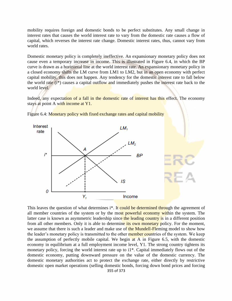
355 of 373

mobility requires foreign and domestic bonds to be perfect substitutes. Any small change in

interest rates that causes the world interest rate to vary from the domestic rate causes a flow of

capital, which reverses the interest rate change. Domestic interest rates, thus, cannot vary from

world rates.

Domestic monetary policy is completely ineffective. An expansionary monetary policy does not

cause even a temporary increase in income. This is illustrated in Figure 6.4, in which the BP

curve is drawn as a horizontal line at the world interest rate. An expansionary monetary policy in

a closed economy shifts the LM curve from LM1 to LM2, but in an open economy with perfect

capital mobility, this does not happen. Any tendency for the domestic interest rate to fall below

the world rate (i*) causes a capital outflow and immediately pushes the interest rate back to the

world level.

Indeed, any expectation of a fall in the domestic rate of interest has this effect. The economy

stays at point A with income at Y1.

Figure 6.4: Monetary policy with fixed exchange rates and capital mobility

This leaves the question of what determines i*. It could be determined through the agreement of

all member countries of the system or by the most powerful economy within the system. The

latter case is known as asymmetric leadership since the leading country is in a different position

from all other members. Only it is able to determine its own monetary policy. For the moment,

we assume that there is such a leader and make use of the Mundell-Fleming model to show how

the leader’s monetary policy is transmitted to the other member countries of the system. We keep

the assumption of perfectly mobile capital. We begin at A in Figure 6.5, with the domestic

economy in equilibrium at a full employment income level, Y1. The strong country tightens its

monetary policy, forcing the world interest rate up to i1*. Capital immediately flows out of the

domestic economy, putting downward pressure on the value of the domestic currency. The

domestic monetary authorities act to protect the exchange rate, either directly by restrictive

domestic open market operations (selling domestic bonds, forcing down bond prices and forcing

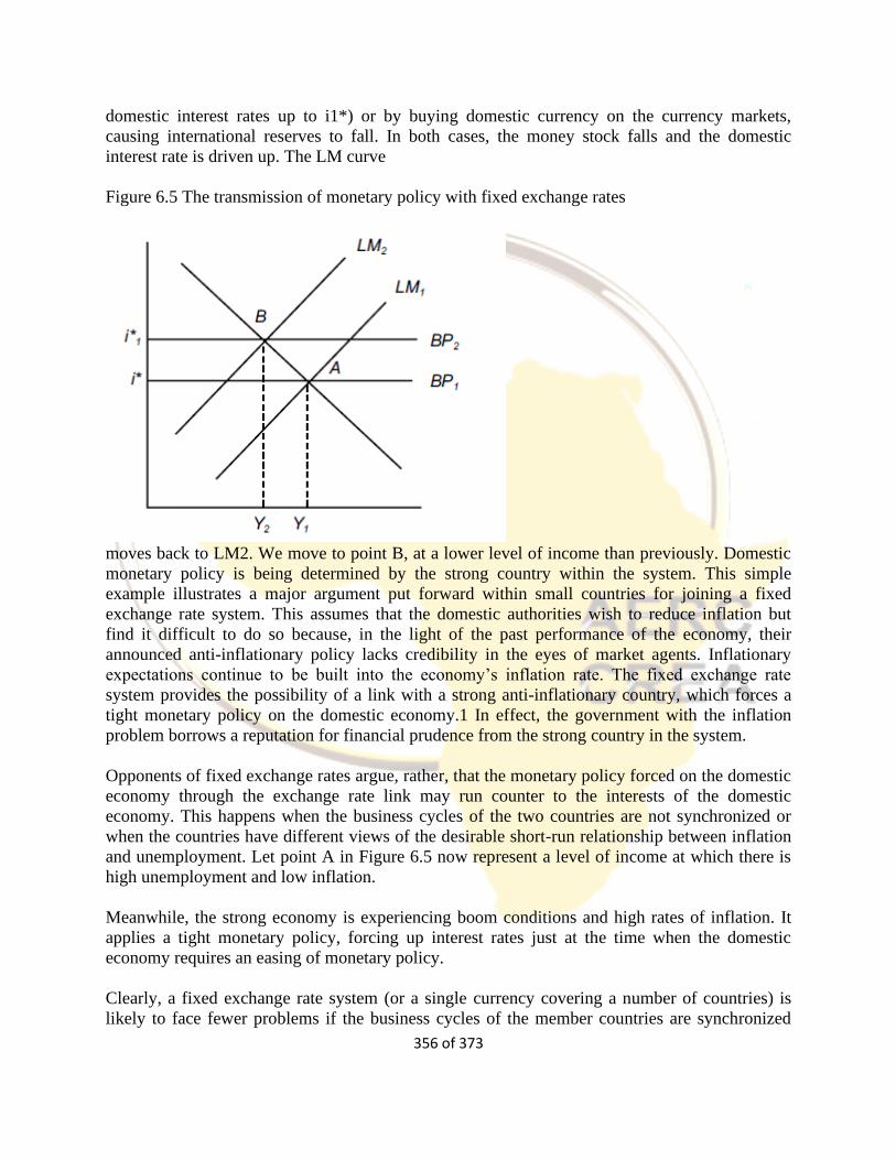
356 of 373

domestic interest rates up to i1*) or by buying domestic currency on the currency markets,

causing international reserves to fall. In both cases, the money stock falls and the domestic

interest rate is driven up. The LM curve

Figure 6.5 The transmission of monetary policy with fixed exchange rates

moves back to LM2. We move to point B, at a lower level of income than previously. Domestic

monetary policy is being determined by the strong country within the system. This simple

example illustrates a major argument put forward within small countries for joining a fixed

exchange rate system. This assumes that the domestic authorities wish to reduce inflation but

find it difficult to do so because, in the light of the past performance of the economy, their

announced anti-inflationary policy lacks credibility in the eyes of market agents. Inflationary

expectations continue to be built into the economy’s inflation rate. The fixed exchange rate

system provides the possibility of a link with a strong anti-inflationary country, which forces a

tight monetary policy on the domestic economy.1 In effect, the government with the inflation

problem borrows a reputation for financial prudence from the strong country in the system.

Opponents of fixed exchange rates argue, rather, that the monetary policy forced on the domestic

economy through the exchange rate link may run counter to the interests of the domestic

economy. This happens when the business cycles of the two countries are not synchronized or

when the countries have different views of the desirable short-run relationship between inflation

and unemployment. Let point A in Figure 6.5 now represent a level of income at which there is

high unemployment and low inflation.

Meanwhile, the strong economy is experiencing boom conditions and high rates of inflation. It

applies a tight monetary policy, forcing up interest rates just at the time when the domestic

economy requires an easing of monetary policy.

Clearly, a fixed exchange rate system (or a single currency covering a number of countries) is

likely to face fewer problems if the business cycles of the member countries are synchronized

357 of 373

and if external shocks to the economies are symmetric — that is, they effect all member

economies in broadly the same way. Another issue of importance is the extent to which monetary

policy has real effects. If monetary policy does not have real effects in the long run, applying the

incorrect monetary policy for a country’s position on its business cycle causes short-run pain but

does not damage the real economy in the long run. However, if there are hysteresis effects, then

the application of a tight monetary policy during a period when the economy is already

experiencing high unemployment increases that unemployment in the short run and results in

long term damage.

The strong country might take some account of the needs of the other members in choosing its

policy. However, if it feels that it would, for political reasons, have to compromise its own policy

preferences too much, the strong country would have little incentive to join the system in the first

place. In any case, if the strong country does take account of the needs of the weaker countries in

determining its policy, it may, by lowering the anti-inflationary credibility of its own monetary

policy, damage the anti-inflation credentials of the system as a whole. This, in turn, would

reduce the potential gains for the small countries from being a member of the system.

The strong country need not adopt an anti-inflationary stance. Expansionary policy is transmitted

through a fixed exchange rate system just as is deflationary policy. Much depends on what gives

the strong country its position within the system. The Bretton Woods adjustable peg exchange

rate system was criticized because the macroeconomic policy of the USA in the later years of the

system’s operation was more inflationary than that desired by other major countries and US

inflation was being transmitted to other countries through the fixed exchange rates. US inflation

made US goods uncompetitive and this, together with the capital outflow resulting from low US

interest rates, produced a balance of payments deficit. The principal trading partners of the USA

found themselves in balance of payments surplus, their international reserves increased and so

did their money stocks.

Brakes on the transmission of monetary influences

Theoretically, countries wishing to follow a less deflationary or less inflationary policy than the

system as a whole, while retaining membership of a fixed exchange rate system may do so by:

devaluing or revaluing the domestic currency, although this needs to conform to the rules of the

system and/or be approved by partner governments; or by

sterilizing the monetary influences spilling over from the policy followed by the strong country.

Let us consider these two possibilities. Countries devaluing their currencies within a fixed

exchange rate system obtain a competitive advantage that produces a current account surplus,

although there may be long time lags in this process.

Countries are, thus, able to maintain a balance of payments balance for any given level of income

at a lower interest rate. The BP curve moves down to BP2, as shown in Figure 6.5. This enables

the authorities to run a more expansionary monetary policy. Interest rates fall (the LM curve

shifts down to LM2), capital flows out of the economy and the current account surplus is offset

by a capital account deficit.

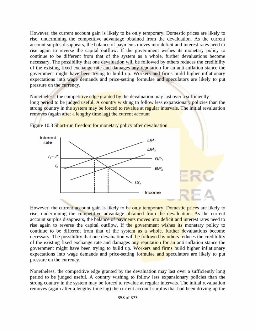
358 of 373

However, the current account gain is likely to be only temporary. Domestic prices are likely to

rise, undermining the competitive advantage obtained from the devaluation. As the current

account surplus disappears, the balance of payments moves into deficit and interest rates need to

rise again to reverse the capital outflow. If the government wishes its monetary policy to

continue to be different from that of the system as a whole, further devaluations become

necessary. The possibility that one devaluation will be followed by others reduces the credibility

of the existing fixed exchange rate and damages any reputation for an anti-inflation stance the

government might have been trying to build up. Workers and firms build higher inflationary

expectations into wage demands and price-setting formulae and speculators are likely to put

pressure on the currency.

Nonetheless, the competitive edge granted by the devaluation may last over a sufficiently

long period to be judged useful. A country wishing to follow less expansionary policies than the

strong country in the system may be forced to revalue at regular intervals. The initial revaluation

removes (again after a lengthy time lag) the current account

Figure 10.3 Short-run freedom for monetary policy after devaluation

However, the current account gain is likely to be only temporary. Domestic prices are likely to

rise, undermining the competitive advantage obtained from the devaluation. As the current

account surplus disappears, the balance of payments moves into deficit and interest rates need to

rise again to reverse the capital outflow. If the government wishes its monetary policy to

continue to be different from that of the system as a whole, further devaluations become

necessary. The possibility that one devaluation will be followed by others reduces the credibility

of the existing fixed exchange rate and damages any reputation for an anti-inflation stance the

government might have been trying to build up. Workers and firms build higher inflationary

expectations into wage demands and price-setting formulae and speculators are likely to put

pressure on the currency.

Nonetheless, the competitive edge granted by the devaluation may last over a sufficiently long

period to be judged useful. A country wishing to follow less expansionary policies than the

strong country in the system may be forced to revalue at regular intervals. The initial revaluation

removes (again after a lengthy time lag) the current account surplus that had been driving up the

359 of 373

country’s reserves and inflating its money supply. Yet this, too, is likely to be only temporary;

meanwhile expectations of further revaluations are likely to reinforce the tendency for capital to

flow in from the inflating economy. The result may be an overall balance of payments balance,

this time with a current account deficit being offset by a capital account surplus. The inflationary

tendencies emanating from the strong economy are countered temporarily but at the expense of

lower output and employment.

Although some policy independence may be granted by occasional exchange rate changes, this

cannot occur as a matter of course. Regular changes in exchange rate parities in a fixed exchange

rate system undermine the system's basis. Firstly, exchange rate uncertainty remains and risk

premiums will be demanded on currencies thought at all likely to devalue.

Secondly, it opens up the possibility of countries seeking to gain advantage through

devaluations. Thus, fixed exchange rate systems must be constructed on the principle that large

changes in exchange rate parities should occur infrequently and should be allowed only if a

country can show that its balance of payments is in ‘fundamental disequilibrium’.2 The ability to

alter exchange rate parities within a fixed exchange rate system can provide only an escape route

for economies in serious difficulties rather than granting monetary policy independence.

A country can also try to avoid inflationary influences from abroad by using domestic monetary

policy to sterilize the impact on domestic money stocks of the inflating economy’s balance of

payments deficit. This operates through the open market sale of government securities, soaking

up excess money balances. Domestic bond prices fall and interest rates rise. The increase in

reserves is offset by the decline in the domestic component of the money stock. The high

domestic interest rate damages investment and, in time, affects both employment and the rate of

economic growth.

Nonetheless, faced with the threat of imported inflation, governments have often chosen

sterilization. It cannot, however, operate effectively in a world with high capital mobility since

the high interest rates attract further capital inflows from abroad, merely compounding the initial

problem.

International capital was sufficiently mobile by the late 1960s to make sterilization difficult for

countries such as Japan, Switzerland, and Germany, which regarded US policy as over-

expansionary. To try to make it work, they had to operate draconian capital controls to limit the

inflow of capital. Countries wishing to avoid deflationary monetary impulses from abroad

without changing their exchange rate parities also require capital controls, this time to prevent

the outflow of capital. In the absence of both exchange rate adjustments and capital controls, the

weak country is constrained to remain at point B in Figure 6.4.

We should not rule out entirely the possibility of operating a fixed exchange rate system with

capital controls. They played an important role in the EMS up until 1991 and have been resorted

to in emergencies since then. However, they are widely regarded as undesirable and have

become increasingly difficult to enforce with the development of offshore financial markets. In

the modern world, they can probably only be enforced for short periods, at best. The difficulties

caused to monetary authorities by the international mobility of capital has led to a call by some

360 of 373

economists for a tax on international capital movements in the hope of slowing them down.

However, even as things are, the chances of some degree of monetary policy independence

within a fixed exchange rate system are not quite as slim as we have so far suggested. In the real

world, even without capital controls, capital is not perfectly mobile. In addition, fixed exchange

rate systems usually allow some freedom for the exchange rate to move around the established

exchange rate parities. There are normally, also, some limitations on the free international flow

of goods and services.

Finally, changes in central parities do not always generate expectations of further changes in the

same direction. Let us consider each of these points briefly.

Capital mobility

Capital is not perfectly mobile internationally unless securities issued in different countries are

considered perfect substitutes for each other across international borders. This may not occur

because of the existence of political or exchange rate risk, different credit ratings of firms and

governments or lack of information on the part of market participants. Any immobility of capital

gives the authorities some opportunity to maintain temporarily an interest rate different from

world rates.

Bands around exchange rate parities

All fixed (but adjustable) exchange rate systems maintain bands around the established central

parities within which market-determined exchange rates may move. These bands may be narrow,

as with the ± 1 per cent of the Bretton Woods system between 1945 and 1971, or broad, such as

the ± 6 per cent for currencies within the broad band of the exchange rate mechanism of the EMS

in operation until July 1993. Following the turmoil in the EMS in that month, an extremely wide

band of ± 15 per cent was adopted, although this was intended to be only temporary and was not

fully used. Its sole purpose was to reduce the scope for profit-making attacks on currencies

by speculators.

The rules of the system may prevent the full use of the band. In the EMS system, currencies were

required to stay within their bands both against the European Currency Unit (Ecu) — a weighted

currency basket consisting of the currencies of all members of the European Union (EU) — and

against each other single currency. This meant in practice that the range of variation before July

1993 was limited to 2.25 or 6 per cent against the strongest or weakest currency in the system.

Further, governments could not allow their currencies to fall to the bottom of the allowed band

since this raised expectations of a possible devaluation and encouraged speculation against the

currency.

Nonetheless, the existence of bands around parities can provide governments with a limited

amount of monetary policy freedom. This applies if the central exchange rates to which the

bands apply are thoroughly credible. Consider Figure 6.6. Here we again assume perfect capital

mobility and show an initial equilibrium with the IS, LM and BP curves intersecting at point A.

We assume this equilibrium to be at the country’s central rate of exchange within a fixed

exchange rate system. BP1 and BP2 show the BP curves that would apply at exchange rates 2.25

361 of 373

per cent above and below the existing central rate. Next we assume that the domestic monetary

authorities expand the money stock, pushing the LM curve down to LM2, intersecting the IS

curve at B, which implies an exchange rate still within the allowable band. In the usual way,

however, the fall in interest rate causes capital to flow out, the money stock falls and the

economy moves back to A.

It remains that B may be a position of short-run equilibrium if it is fully believed that the

exchange rate will move back to its original position. The expected increase in the value of the

currency causes agents to be willing to hold the currency even at a rate of interest temporarily

below the world level.

If the value of the domestic currency stays below its central rate for any length of time,

expectations of a movement back to the central rate begin to be undermined and capital again

begins to flow out, leading to expectations of a future devaluation. Thus, the degree of

independence of domestic monetary policy granted by the existence of bands around central rates

of exchange is strictly limited and conditional, but some short-run freedom is provided and this

freedom is greater the wider is the band.

Limitations on free trade

Some freedom may be retained also through the ability of a government to protect the current

account of its balance of payments using commercial policy (tariffs, quotas and other non-tariff

barriers). Although the capital account is a much more potent source of instability, expectations

of devaluation are often triggered by current account weakness. Extra tension was caused in the

EMS in the early 1990s because of the move (under the Single European Act of 1986) towards a

unified market within the EU, severely limiting the ability of member governments to protect

their current accounts through trade restrictions as well as leading to the removal of restrictions

on capital movements within the EU.

Expectations of future devaluations following a devaluation

Finally, one devaluation does not always convince the financial markets that others will follow.

Consider a case in which a country maintains a fixed parity for an extended period but steadily

loses competitiveness over that period. Its rate of inflation may be converging on that of the

strong country within the system, but only slowly. Under these circumstances, many come to

appreciate that the existing parity cannot be maintained and that devaluation is necessary to

restore competitiveness. The secret is either to make small adjustments to the exchange rate

when needed, such that each change does not engender significant inflationary expectations

and/or to accompany the devaluation with other policies aimed at preserving the credibility of the

government’s anti-inflationary stance.

362 of 373

Figure 6.6: Monetary policy in a fixed exchange rate system

To sum up this section, we can refer to the ‘inconsistent quartet’,4 which states that governments

cannot at the same time maintain all of the following:

• free trade

• full capital mobility

• fixed exchange rates

• national autonomy in the conduct of monetary policy.

This does not apply to the strong country of the system, which is able to determine its own

monetary policy, as long as it is able to withstand the political pressure emanating from other

members in cases where interests conflict.

Monetary policy with floating exchange rates

Our limited analysis earlier in this section concluded that monetary policy was more effective in

an open economy with floating exchange rates than in a closed economy for two reasons:

the exchange rate freedom grants the economy monetary independence and allows the authorities

to choose the domestic inflation rate;

the exchange rate movements have an impact on the real economy by changing the international

competitiveness of the country’s output.

Thus, an increase in the money supply causes income to rise and the interest rate to fall. The

increase in income causes a deterioration in the current account in the balance of payments while

the fall in interest rate causes a deterioration in the capital account. There is a net outflow of

currency (the supply of domestic currency increases) and the exchange rate depreciates.

The depreciation improves the international competitiveness of domestically produced goods and

this causes a further increase in income.

This analysis implied that the exchange rate changed to restore the goods and money markets

and the balance of payments to equilibrium. Income, then, increases, but the size of any real

effects of monetary policy depends on the extent to which this reflects an increase in the price

363 of 373

level, rather than output. This, in turn, depends on the extent of the depreciation that follows the

monetary expansion. If the value of the currency falls in proportion to the increase in the money

supply, the full weight of the expansion falls on the price level. There are no real effects. Money

is neutral. To allow us to say more about this, we need to look briefly at theories of the

determination of exchange rates in floating exchange rate systems.

The simplest model of exchange rate determination is the flexible price monetary model. This

assumes that capital is perfectly mobile (domestic and foreign bonds are perfect substitutes),

markets are competitive, trans actions costs are negligible, and investors hold exchange rate

expectations with certainty. Uncovered interest rate parity (UIRP) holds — that is, the expected

rate of depreciation of a currency equals the interest rate differential between domestic and

foreign bonds. Thus, if the interest rate on UK bonds were two per cent above the interest rate on

US bonds, investors would expect sterling to depreciate by two per cent against the dollar. The

key determinants of exchange rates are the supply of and demand for money.

We assume, also, that all prices are perfectly flexible. Purchasing power parity (PPP) holds and

money markets clear continuously. The demand for money is stably related to real income and

stably and negatively related to the rate of interest.

m − p = ηy − si

where m is the log of the domestic money stock, p is the log of the domestic price level, y is the

log of domestic real income, and r is the rate of interest. The same relationship holds abroad and

thus:

m* − p* = ηy* − si*

Since PPP is assumed, we can write:

s = p − p*

where s is the exchange rate. Further, since UIRP holds, we have:

Es = i − i*

(the expected rate of depreciation of the home currency equals the difference between the

domestic and foreign interest rates).

Re-arranging and substituting in 10.3 gives:

s = (m − m*) − η(y − y*) + σ (i − i*)

That is, the rate of exchange is determined by the supply of money and the demand for money

function at home and abroad.

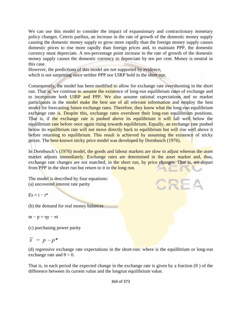
364 of 373

We can use this model to consider the impact of expansionary and contractionary monetary

policy changes. Ceteris paribus, an increase in the rate of growth of the domestic money supply

causing the domestic money supply to grow more rapidly than the foreign money supply causes

domestic prices to rise more rapidly than foreign prices and, to maintain PPP, the domestic

currency must depreciate. A ten-percentage point increase in the rate of growth of the domestic

money supply causes the domestic currency to depreciate by ten per cent. Money is neutral in

this case.

However, the predictions of this model are not supported by evidence,

which is not surprising since neither PPP nor UIRP hold in the short run.

Consequently, the model has been modified to allow for exchange rate overshooting in the short

run. That is, we continue to assume the existence of long-run equilibrium rates of exchange and

to incorporate both UIRP and PPP. We also assume rational expectations and so market

participants in the model make the best use of all relevant information and employ the best

model for forecasting future exchange rates. Therefore, they know what the long-run equilibrium

exchange rate is. Despite this, exchange rates overshoot their long-run equilibrium positions.

That is, if the exchange rate is pushed above its equilibrium it will fall well below the

equilibrium rate before once again rising towards equilibrium. Equally, an exchange rate pushed

below its equilibrium rate will not move directly back to equilibrium but will rise well above it

before returning to equilibrium. This result is achieved by assuming the existence of sticky

prices. The best-known sticky price model was developed by Dornbusch (1976).

In Dornbusch’s (1976) model, the goods and labour markets are slow to adjust whereas the asset

market adjusts immediately. Exchange rates are determined in the asset market and, thus,

exchange rate changes are not matched, in the short run, by price changes. That is, we depart

from PPP in the short run but return to it in the long run.

The model is described by four equations:

(a) uncovered interest rate parity

Es = i − i*

(b) the demand for real money balances

m − p = ηy − σi

(c) purchasing power parity

(d) regressive exchange rate expectations in the short-run: where is the equilibrium or long-run

exchange rate and θ > 0.

That is, in each period the expected change in the exchange rate is given by a fraction (θ ) of the

difference between its current value and the longrun equilibrium value.

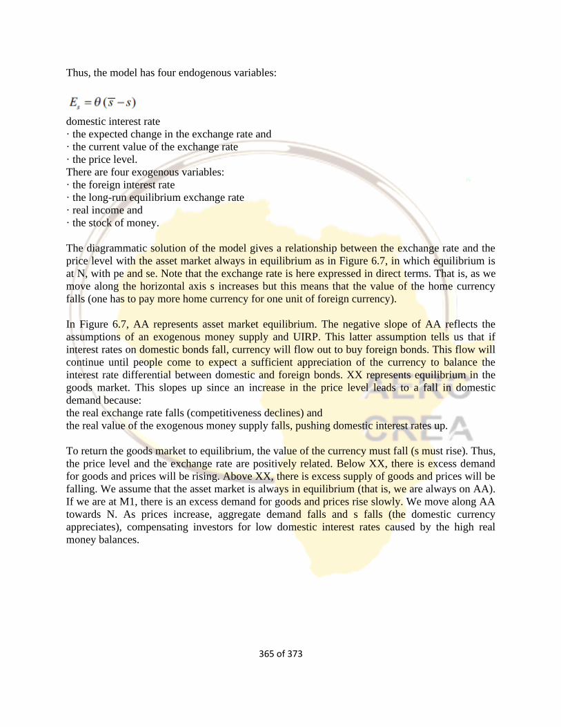
365 of 373

Thus, the model has four endogenous variables:

domestic interest rate

· the expected change in the exchange rate and

· the current value of the exchange rate

· the price level.

There are four exogenous variables:

· the foreign interest rate

· the long-run equilibrium exchange rate

· real income and

· the stock of money.

The diagrammatic solution of the model gives a relationship between the exchange rate and the

price level with the asset market always in equilibrium as in Figure 6.7, in which equilibrium is

at N, with pe and se. Note that the exchange rate is here expressed in direct terms. That is, as we

move along the horizontal axis s increases but this means that the value of the home currency

falls (one has to pay more home currency for one unit of foreign currency).

In Figure 6.7, AA represents asset market equilibrium. The negative slope of AA reflects the

assumptions of an exogenous money supply and UIRP. This latter assumption tells us that if

interest rates on domestic bonds fall, currency will flow out to buy foreign bonds. This flow will

continue until people come to expect a sufficient appreciation of the currency to balance the

interest rate differential between domestic and foreign bonds. XX represents equilibrium in the

goods market. This slopes up since an increase in the price level leads to a fall in domestic

demand because:

the real exchange rate falls (competitiveness declines) and

the real value of the exogenous money supply falls, pushing domestic interest rates up.

To return the goods market to equilibrium, the value of the currency must fall (s must rise). Thus,

the price level and the exchange rate are positively related. Below XX, there is excess demand

for goods and prices will be rising. Above XX, there is excess supply of goods and prices will be

falling. We assume that the asset market is always in equilibrium (that is, we are always on AA).

If we are at M1, there is an excess demand for goods and prices rise slowly. We move along AA

towards N. As prices increase, aggregate demand falls and s falls (the domestic currency

appreciates), compensating investors for low domestic interest rates caused by the high real

money balances.

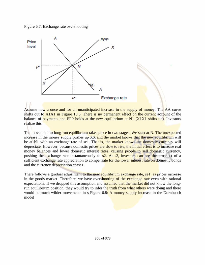
366 of 373

Figure 6.7: Exchange rate overshooting

Assume now a once and for all unanticipated increase in the supply of money. The AA curve

shifts out to A1A1 in Figure 10.6. There is no permanent effect on the current account of the

balance of payments and PPP holds at the new equilibrium at N1 (X1X1 shifts up). Investors

realize this.

The movement to long-run equilibrium takes place in two stages. We start at N. The unexpected

increase in the money supply pushes up XX and the market knows that the new equilibrium will

be at N1 with an exchange rate of se1. That is, the market knows the domestic currency will

depreciate. However, because domestic prices are slow to rise, the initial effect is to increase real

money balances and lower domestic interest rates, causing people to sell domestic currency,

pushing the exchange rate instantaneously to s2. At s2, investors can see the prospect of a

sufficient exchange rate appreciation to compensate for the lower interest rate on domestic bonds

and the currency depreciation ceases.

There follows a gradual adjustment to the new equilibrium exchange rate, se1, as prices increase

in the goods market. Therefore, we have overshooting of the exchange rate even with rational

expectations. If we dropped this assumption and assumed that the market did not know the long-

run equilibrium position, they would try to infer the truth from what others were doing and there

would be much wilder movements in s Figure 6.8: A money supply increase in the Dornbusch

model

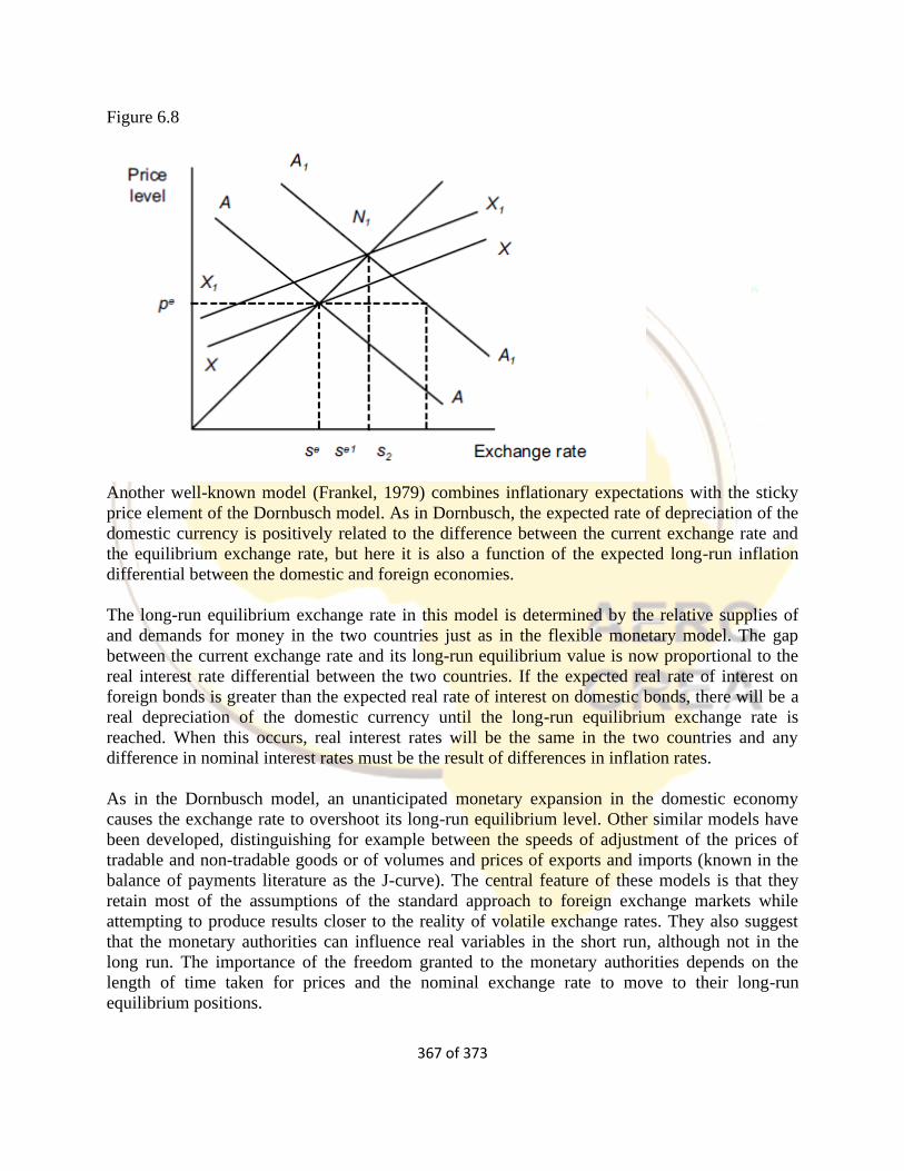
367 of 373

Figure 6.8

Another well-known model (Frankel, 1979) combines inflationary expectations with the sticky

price element of the Dornbusch model. As in Dornbusch, the expected rate of depreciation of the

domestic currency is positively related to the difference between the current exchange rate and

the equilibrium exchange rate, but here it is also a function of the expected long-run inflation

differential between the domestic and foreign economies.

The long-run equilibrium exchange rate in this model is determined by the relative supplies of

and demands for money in the two countries just as in the flexible monetary model. The gap

between the current exchange rate and its long-run equilibrium value is now proportional to the

real interest rate differential between the two countries. If the expected real rate of interest on

foreign bonds is greater than the expected real rate of interest on domestic bonds, there will be a

real depreciation of the domestic currency until the long-run equilibrium exchange rate is

reached. When this occurs, real interest rates will be the same in the two countries and any

difference in nominal interest rates must be the result of differences in inflation rates.

As in the Dornbusch model, an unanticipated monetary expansion in the domestic economy

causes the exchange rate to overshoot its long-run equilibrium level. Other similar models have

been developed, distinguishing for example between the speeds of adjustment of the prices of

tradable and non-tradable goods or of volumes and prices of exports and imports (known in the

balance of payments literature as the J-curve). The central feature of these models is that they

retain most of the assumptions of the standard approach to foreign exchange markets while

attempting to produce results closer to the reality of volatile exchange rates. They also suggest

that the monetary authorities can influence real variables in the short run, although not in the

long run. The importance of the freedom granted to the monetary authorities depends on the

length of time taken for prices and the nominal exchange rate to move to their long-run

equilibrium positions.

368 of 373

Expansionary monetary policy could obtain worthwhile reductions in unemployment for

significant periods. If a sticky-price model were combined with a labour market model with

hysteresis, these short-run employment gains could become long-run gains. Sticky-price models

also provide a justification for a gradual approach to monetary policy. For example, assume the

monetary authorities wish to reduce the rate of inflation. If they reduce the rate of growth of the

money supply sharply and interest rates rise, but prices do not change in the short run, the

nominal and real exchange rates fall sharply (overshooting the long-run equilibrium level),

causing problems for exporters and import-competing industries. Unemployment results. If

prices were slow to change, these real problems would persist for a considerable time. The

position would be worse if the short-run overvaluation of the currency caused bankruptcies of

domestic firms and serious loss of market share in important industries. The short-run cost of

reducing inflation could be high. This leads to the view that monetary policy should be applied

gradually to allow the economy to adjust slowly.

There remain two problems with sticky price models from the point of view of monetary policy.

Firstly, although PPP does better in long run than in short run tests, the evidence that it holds in

the long run is not convincing. This increases the strength of the argument that monetary policy

in an open economy has a long run impact on real variables. Secondly, all monetary models do

not allow a distinction to be made between open market and foreign exchange operations.

Suppose the monetary authorities seek to improve the country’s competitiveness by lowering the

value of the currency. They buy foreign bonds with domestic currency, increasing the supply of

the domestic currency on the market. The exchange rate of the domestic currency rises (its value

falls) and the current account of the balance of payments improves.

However, the country’s holding of foreign exchange reserves increases and the money supply

rises, creating inflationary pressure. The inflation then removes the competitive advantage

obtained from the higher exchange rate of the domestic currency. The monetary authorities aim

to counter this by selling domestic bonds to reduce the domestic component of the money stock.

Consider this in terms of equation 7.2 :

M = D + R

The authorities attempt to increase R and reduce D so that the money supply does not change,

but the exchange rate does, but this type of operation is not possible within the framework of a

monetary model of exchange rate determination because domestic and foreign bonds are perfect

substitutes.

Changes in D and R have equivalent effects on the exchange rate. This is another way of saying

that in a monetary model, the monetary authorities cannot influence the real exchange rate

(except in the short-run, in sticky price models).

Portfolio models of the exchange rate overcome this by dropping the assumption that foreign and

domestic bonds are perfect substitutes. Uncovered interest rate parity does not apply. We assume

that residents of the domestic economy think foreign bonds are more risky than equivalent

domestic bonds and hence require a higher rate of interest on foreign bonds to be persuaded to

hold them. This inclusion of differential risk in the analysis allows open market operations and

369 of 373

foreign exchange operations to have different effects on interest rates and exchange rates, and

introduces the possibility of monetary authorities making use of sterilized foreign exchange

operations. Monetary authorities now have a wider choice of policy actions.

We have so far seen that with mobile capital the following applies:

(a) in fixed exchange rate systems, the target of monetary policy is the

exchange rate — domestic inflation rates are determined by the monetary

policy of the whole system;

(b) in floating rate systems, the monetary authorities can target the domestic rate of inflation.

In practice, however, exchange rates in floating exchange rate systems do not float freely.

Central banks intervene to varying degrees to influence exchange rates. Sometimes the

intervention is light, with the intention only of smoothing out fluctuations in exchange rates. On

other occasions, central banks join together to intervene strongly in the foreign exchange market

in the hope of influencing the direction in which exchange rates are moving or to try to keep

rates within unspecified target ranges. In this case, monetary policy may be aimed either at

internal or at external objectives.

1.6.4 The Policy Mix and Monetary Policy Coordination

One of the standard arguments for floating exchange rates is that they isolate an economy from

external shocks, allowing the authorities to pursue their own independent monetary policy.

However, it has become clear that all economies are interdependent and are subject to spillovers

from the domestic monetary policies of other economies. Further, the degree of interdependence

among countries has been growing. This happened particularly in the early 1970s because of:

• increased capital flows after the collapse of the Bretton Woods fixed exchange rate

system

• alterations in terms of trade following large changes in world oil Prices a greater degree

of openness to foreign trade and the development of offshore financial markets.

Our particular interest here is in what has been called ‘sensitivity independence’, defined by

Cooper (1985) as the amount of adjustment a country has to make to foreign events under

conditions of normal economic activity. This is determined by factors such as the marginal

propensities to spend on foreign products or assets, the elasticity of substitution between foreign

and domestic products or assets, the elasticity of substitution in production and the relative size

of the economies in question. The theoretical approach to macroeconomic policy coordination

calls upon a number of areas of macroeconomic theory, as well as making use of games theory to

incorporate in models the notions of credibility and reputation, and the sustainability

and time consistency of policy.

The first stage in the analysis of macroeconomic interdependence among economies was the

investigation of the channels along which influence flows from one economy to another. The

370 of 373

beginnings of a case for some form of policy coordination can be derived from the simple open

economy multiplier. For a small economy, it is clear that increased linkages with them rest of the

world weaken the impact on domestic targets of domestic fiscal policy. Models can, however, be

greatly complicated by dropping the small country limitation, by making different assumptions

about the nature of the exchange rate regime, by introducing various forms of price or wage

stickiness, or by considering the timing and nature of tax policy changes needed to pay for

government expenditure increases.

The analysis of monetary linkages builds on the Mundell-Fleming model, making varying

assumptions about the exchange rate regime, the degree of international capital mobility, and

country size. Depending on the assumptions made, spillovers from domestic macroeconomic

policy may be positive or negative. The importance of spillovers became clearer, however, with

the recognition of price spillovers operating through the terms of trade linkage (Hamada, 1976).

This plainly meant the end of arguments that a country could fully insulate itself from events and

policies in the rest of the world. Even with perfectly flexible exchange rates, the terms of trade

transmission works.

Cooper (1969) examined the impact of spillovers on domestic policy using a simple model with

fixed exchange rates and constant prices. He argued that the greater is the degree of

interdependence (and the stronger are spillovers), the less will be the effectiveness of policies in

non-cooperating economies. Greater interdependence, in other words, leads to either worse

results from domestic policies and longer periods away from equilibrium, or greater costs to

restore targets to their desired values.

In Canzoneri and Gray’s (1985) model, the governments of two identical countries both attempt

to achieve full employment output without increasing inflation. Both countries are subject to

supply shocks. The paper is concerned with the monetary transmission mechanism, specifically

with the impact of an expansion of the money supply in each country. Canzoneri and Gray

consider three possibilities:

(a) beggar-thy-neighbour in which monetary expansion in one economy has a negative effect on

output in the other economy

(b) locomotive in which the spillover effects are positive and

(c) asymmetric in which monetary spillovers have different signs, the result depending on the

size of the exchange rate and interest rate changes following the domestic monetary expansion as

well as the import content of the foreign price index. The outcome is an empirical question,

depending on the structure of the economies involved.

It has been shown that it is possible both for an instrument’s spillovers to change signs over time

and for an instrument to have impacts of different signs depending on the target at which it is

aimed. Specific conclusions of theoretical models must, however, be treated with caution since

many depend on the sign or relative size of particular coefficients while the models assume that

the economy's behavioural parameters are unchanged under different conditions. They thus

founder on the Lucas critique. In addition, there have not been enough empirical studies to

produce clear ideas about the likely direction and size of spillovers in practice. We are only left,

following Hughes-Hallett (1989), with a set of not very surprising theoretical conclusions:

371 of 373

• Spillovers vary with the policies pursued in other countries

• There are multiple transmission mechanisms that operate simultaneously

• Net spillover effects depend on the particular circumstances of the economies concerned

• The impacts of spillovers crucially depend on the size of the economy, the degree of asset

substitutability, relative price and wage flexibility and exchange rate flexibility.

Games theory has been used to analyze the desirability of policy coordination. This commenced

with the development of models incorporating two simple forms of policy decisions by national

governments in an international context — Nash non-cooperative games in which either

governments act independently taking the decisions of other governments as given or one

country acts as leader; and cooperative games in which countries attempt to pursue some

common interest, attempting to maximize the sum or product of the utilities of the national

governments. The problem is to elucidate and, if possible, to quantify the gains from co-

operative decisions.

Non-cooperative models suffer from a variety of defects. For example, they consider only static

decisions and thus allowance cannot be made for predictable future effects of current decisions.

Further, the restrictions on the assumptions regarding the behaviour of the other country’s policy

makers presupposes that policy makers already know the form of the equilibrium decision rule:

but this can only be so in special circumstances. Despite

these difficulties, the sub-optimality of non-cooperative decisions is accepted. The presence of

significant policy spillovers forms the basis of a wellknown model (Hamada 1976, 1985)

illustrating the case for international policy coordination between countries. It is a two-country

model, with each country targeting its inflation rate and balance of payments position in a

fixed exchange rate regime. Each country controls a single policy instrument — the level of

domestic credit creation. Neither country can attain both objectives by acting alone except by

coincidence. In one version of this model with demand-constrained output and price inertia,

Nash noncooperative behaviour gives the system a deflationary bias. Coordination is clearly

preferable.

This fits in with the general conclusion that non-cooperative decisions are socially inefficient

except under special conditions.

However, it is one thing to argue for the inefficiency of non-cooperation, but quite another to

accept the need for coordination. To begin with, one can produce cases where Nash non-

cooperative behaviour is superior to cooperation. Perhaps the best-known example of this is

Rogoff’s international inflation game in which governments gain from unexpected inflation

(Rogoff, 1985b). In Rogoff’s model, governments fix exchange rates and then agree to raise their

domestic money supplies. By cooperating, they are able to exploit the gains to be had from

inflation surprises. Their citizens lose out. This assumes that the private sector can be taken by

surprise.

Most models rule this possibility out by assuming forward-looking expectations. Without

surprises, the costs to the private sector of anticipated inflation remain, but an understanding of

the nature of government policy by the private sector leads to a rapid reduction in their

willingness to hold government debt except at interest rates that fully take government policy

372 of 373

into account. One can also show that the degree of sub-optimality of non-cooperative

decisions can be affected by the strength of preferences of national policy makers, by the

economy’s policy responses, and by capacity constraints.

We can only conclude that the size of net gains (or losses) from cooperation can only be

determined by empirical analysis. In attempting to bridge the gap, however, between theory and

reality, economic theory has paid most attention to a different set of difficulties — if

governments succeed in reaching an agreement to coordinate macroeconomic policies, how can

we be sure that such policies will be sustained in each country? There are two separate issues

here.

The first deals with the relationship between the state and the private sector.If rational

expectations are assumed and thus the private sector cannot be taken by surprise by the

government, the effectiveness of macroeconomic policy depends on that policy being credible to

the private sector. If this is not the case, macroeconomic policy is ineffective. One way out for

governments is to pre-commit themselves to their stated policy. An obvious example is the pre-

commitment of monetary policy through membership of a fixed exchange rate regime as long as

the exchange rate parity is itself credible.

The second issue relates to the temptation felt by governments to renege on their agreements

with other governments. The issue hardly arises in the Hamada two-country model since an

attempt by one country to improve its position by reneging on the agreement will be met by a

withdrawal of the other country from the agreement — both countries move back to the original

sub-optimal non-cooperative equilibrium and are worse off. The threat of such action prevents

either country from reneging. However, with more than two participants, the question of the

credibility of threats becomes relevant.

Where the incentive to renege on agreements cannot be removed by credible threats to retaliate,

policy coordination cannot be sustained. There are two ways out of this dilemma. The first is to

concentrate on the notion of reputation. Governments may adopt a longer term view of

coordination than is implied by the one-off bargains that dominate the world of policy models.

Consequently, they may be willing to forgo potential short-term gains available from reneging on

agreements in order to make future bargains possible. Yet again, the loss of reputation in the

field of macroeconomic policy coordination might be thought likely to affect a country’s

standing in other international negotiations. This is an example of the problems involved in

analysing macroeconomic policy in isolation. It is clear that the outcomes of G7 economic

summits have been influenced by much more than narrow macroeconomic considerations.

The second way out is to develop arguments in favour of rule-based\ rather than discretionary

policy coordination. The acceptance of rules means that all governments are pre-committed to

agreed polices, removing the dangers apparent in cases where some parties are effectively pre-

committed but others are not. A considerable number of empirical studies have been undertaken.

These have produced mixed results regarding the benefits from macroeconomic policy

coordination. On balance, where studies have shown gains from coordination, they have tended

to be rather small, although the gains appear to increase with the persistence of disturbances that

373 of 373

lead to coordination.

They also appear to increase over time. In the long run, gains from cooperation in the face of

permanent supply or demand shocks may be very considerable. Such studies are of some interest

in themselves but the ability of researchers to vary the results by making relatively small changes

in their models means that they can, at best, provide only luke-warm support for policy

coordination.