Aerospace Science and Technology 63 (2017) 294–303

Contents lists available at ScienceDirect

Aerospace Science and Technology

www.elsevier.com/locate/aescte

Behaviour of trailing wing(s) in echelon formation due to wing twist

and aspect ratio

M. Gunasekaran ∗, Rinku Mukherjee

Indian Institute of Technology Madras, 600036, India

a r t i c l e i n f o a b s t r a c t

Article history:Received 1 August 2016Received in revised form 13 January 2017Accepted 16 January 2017Available online 17 January 2017

Keywords:Formation flyingGeometric twistAerodynamic twistInduced dragPost-stall flows

In this paper, a novel decambering technique has been implemented using a vortex lattice method to study the effects of wing twist on the induced drag of individual lifting surfaces in configuration flight including post-stall angles of attack. The effect of both geometric and aerodynamic twist is studied. In the present work, 2D data of NACA0012 airfoil from XFoil at Re = 1 × 106 is used to predict 3D post-stall data using geometric twist for a single wing and compared with literature. The effect of aerodynamic twist is implemented by using different airfoils along wing–span and the resulting wing CL–α and Cdi–αare compared with experiment. Study of wings of different aspect ratios with & without aerodynamic twist on both leading and trailing wings helps to understand the effect of twist on the lift and induced drag when they are varied on both wings simultaneously and individually.

© 2017 Elsevier Masson SAS. All rights reserved.

1. Introduction

Formation flight has seen considerable interest in the research community due to its promise of fuel savings due to reduced drag. In this work, the numerical technique that we use gives aero-dynamic data for a wider variety of possibilities in a formation, namely the shape and size of individual wings. The method used works at post-stall angles of attack and interesting behaviour is noted when one or more wings in a formation operates at these regions of flow. The modelling technique used also enables to gen-erate results very quickly.

The drag reduction in a formation is due to the trailing wing operating in the downwash region of the leading wing. In this work, we have used a twisted leading wing to study the effects on the trailing wing. We have also changed the size of the leading wing (aspect ratio) to study its changes on the trailing wing.

Using a twisted leading wing essentially changes the distribu-tion of the effective angle of attack on the trailing wing and using different aspect ratios of the leading wing changes the location of the tip vortices, which effect the behaviour of the trailing wing.

In the present work, analysis at post-stall angles of attack shows that stall can be pre-poned or post-poned depending upon the formation. The objective and motivation for this work stems from the fact that all facets of formation can be analysed and such

* Corresponding author.E-mail address: aerogunasekar@gmail.com (M. Gunasekaran).

http://dx.doi.org/10.1016/j.ast.2017.01.0091270-9638/© 2017 Elsevier Masson SAS. All rights reserved.

knowledge and information can serve as the basis of design of for-mations.

In previous work, we have shown the effect of changing offsets (dx, dy, dz) and angles of attack of the wings on a formation [1].

As per the history of formation flying, the early research started in the year 1914 by Weiselsberger [2] who calculated the induced drag which could be reduced by velocity field and induced by bound & trailing vortices of nearby flock members. The horseshoe vortex of constant strength was replaced by a bird and three birds were considered in a diagonal–line formation. The sample calcula-tion showed that the bird in the middle position gains 15.2% drag reduction.

Schlichting [3] analysed the formation flight and studied the in-teraction of multiples airplanes using horse shoe vortices for V and inverted V formations. The first calculation on fuel savings have been made in symmetrical formations of airplanes Ju 52 which was used by German airforce during WW II. The rates of energy savings have been calculated for various aircraft numbers and rec-ommended inverted V-formations for practical reasons, i.e. visibil-ity and evenly drag distribution.

D. Hummel [4] conducted a survey on formation flight of birds by doing study on three types problems which turned out all three can’t be solved directly by measurements on birds and aerody-namic forces acting on birds in soaring flight or flapping flight can’t be determined by wind-tunnel experiments. He also con-cluded that possible approach is only by quantitative experimental investigation of the position and motion of the birds in flight and subsequent analysis by means of aerodynamic theory.

M. Gunasekaran, R. Mukherjee / Aerospace Science and Technology 63 (2017) 294–303 295

Nomenclature

Cl(sec) 2D section coefficient of liftCm(sec) 2D section coefficient of pitching momentCdi(sec) 2D section coefficient of induced dragCL(max) maximum Lift coefficientCdi(min) minimum Induced Drag coefficientCL 3D wing coefficient of liftCm 3D wing coefficient of momentC Di 3D wing coefficient of induced drag(L/D)max maximum lift-to-drag ratioc wing chord lengthLLT lifting line theoryV LM vortex–lattice method

Subscript

α angle of attack

αCL=0 zero-lift angle of attack�Cl,�Cm Difference between viscous and potentialδ1, δ2 decambering functions(x1, x2) Cartesian locations of δ1 and δ2

(θ1, θ2) spherical locations of δ1 and δ2

max maximumlw leading wingt w trailing wingsec sectionvisc viscousAR aspect ratiodx chord-wise offsetdy span-wise offsetdz vertical offset

The benefits gained by birds in formation remains same for fixed wing aircrafts. Markus Beukenberg & Dietrich Hummel [5]analysed and proved that when two airplanes Do-28 flies in forma-tion, a maximum flight power reduction of about 15% is achievable for the rear aircraft at very small lateral distances.

In our present work, wing twist is applied in single and mul-tiple wing configurations. The benefits of applying wing twist are studied both by geometric and aerodynamic twist. The further lit-erature shows how wing twist was applied in the past in different applications.

Wing–twist distribution is not the least controversial design pa-rameter and has to be carefully selected so that the cruise drag is not excessive. In a rectangular wing, the washout due to wing–twist causes the root to stall before the wing tips. The solution based on washout optimization using lifting line theory [6] gives the idea of how to minimize the induced drag at a design CL ef-fectively by using both geometric and aerodynamic twist.

It has been shown that any planform shape may be opti-mized with wing–twist to reduce the induced drag to an optimum value [7]. They have been shown that the maximum lift–drag ra-tio increases and the maximum CL reduces as the distance be-tween the wing root and the twist start line decreases. They also mentioned that twist could be applied only on the area of the wingspan, and the effect of the twist on CLmax and (L/D)max could be reduced.

Lingxiao Zheng [8] used many models to study the wing and body kinematics of painted lady butterfly. It may be noted that the twist-only-wing (TOW) model recovers much of the perfor-mance of observed butterfly wing (OBW) model by demonstrating the wing–twist but, not the camber is the key to forward flight in these insects.

Geoffrey et al. [9] used the LinAir, a discrete vortex Weissen-ger program to analyze the representative aircraft and formation geometries. In order to get desirable load distributions the wings of three different models were twisted. In LinAir calculations they used the DC-10-30 wing geometry, assumed a streamwise spacing between aircraft of (x/b) = 5.0 and no vertical gap was used.

Ashok Gopalarathnam [10] concluded that to achieve elliptical loading (or any other target loading) when flying in a formation, a wing must have the freedom to adapt its shape via twist or con-trol deflections. He also said that birds are able to achieve this by wing–shape adaptation using some form of aerodynamic sensing.

H.P. Thien et al. [11] used domain discretization and flow field properties evaluation to explain the effect of incidence angle, dihe-dral angle, aspect ratio and taper ratio in V-formation flight. They found that aspect ratio has a significant effect on increasing the

rear wing lift and pitching moment, but seems to be no effect to the drag reduction.

Sara Nichols [12] explains how reduction in washout at the highest rate of wing twist lowers the direct span-wise strains in the outboard section of the rib and the consequent reduced shear strains induced by the coupling terms. They also have explained how aerodynamic subroutine optionally calculates the required amount of twist for various sections along the aerofoil that would achieve an elliptical lift distribution for a given set of user input parameters. Twist changes the structural weight by modifying the moment distribution over the wing.

Kevin et al. [13] introduced a new way of giving aerodynamic twist to the wing by finding the set of spanwise locations and their corresponding design lift coefficients that minimize the error between the CL distribution achieved by aerodynamic twist and the CL distribution resulting from the desired lift distribution and planform shape. Similarly, geometric twist is given by superimpos-ing all the �CL .c distributions due to each twist distribution to calculate the required twist function weights.

The wind-tunnel test was conducted by Vanessa L. Bond et al. [14] to demonstrate the use of wing twist for longitudinal (pitch) control in a joined-wing-aircraft configuration and to val-idate models that are used in analysis methods. They also investi-gated the feasibility of incorporating flexible twist for pitch control in the design of a high-altitude long-endurance aircraft.

Ivan Korkischko et al. [15] examined the application of forma-tion flight to micro air vehicles with regard to possible power savings. They also stated that the effect of the induced upwash can be seen as a modification of wing twist, which is used to optimize the spanwise lift distribution on nonelliptic planforms to lower the induced drag for a given lift value.

2. Numerical procedure

A vortex–lattice method algorithm based on the decambering approach [16] is used for predicting formation flight aerodynamics of wings using known section data. Although the numerical code, VLM3D based on this approach was originally developed with a view to predict post-stall aerodynamics of single wings or their configurations, it has been found to be robust and powerful in the analysis of formation flight as well with some modifications.

The ability to change spatial offsets (chord-wise, span-wise and vertical), the ability to change the angle of attack of the trailing aircraft for a particular angle of attack of the leading aircraft and vice versa are incorporated into VLM3D to study formation flight aerodynamics. The unique feature of formation flight is the inter-

296 M. Gunasekaran, R. Mukherjee / Aerospace Science and Technology 63 (2017) 294–303

action between the vortices and aircrafts (both leading and trail-ing), which is captured well by the modified VLM3D [1]. Post-stall results provide enhanced understanding of formation flight aero-dynamics.

For the current work, further functionalities have been incorpo-rated into VLM3D, which include the ability to change wing twist, both geometric and aerodynamic and also by using different air-foils along span.

The code VLM3D based on the decambering approach was de-veloped wherein the chordwise camber distribution at each section of the wing was reduced to account for the viscous effects at high angles of attack. The approach uses either or both Cl and Cm sec-tion data and uses a two-variable function for the decambering. In addition, unlike all earlier methods, the approach uses a multi-dimensional Newton iteration that accounts for the cross-coupling effects between the sections in predicting the decambering for each step in the iteration. The subsequent discussion illustrates briefly the decambering approach by describing its application to model a two-dimensional flow past an example airfoil. The itera-tive approach for three-dimensional geometries is discussed next.

2.1. Application to 2D flow

The overall objective was to arrive at a scheme for incorporating the nonlinear section lift curves in wing analysis methods such as Lifting line theory (LLT), discrete-vortex Weissinger’s method and vortex lattice methods. For this purpose, it was assumed that the two-dimensional data Cl–α and Cm–α for the sections forming the wing were available from either experimental or computational re-sults. The objective was that for the final solution of the 3D flow, the � distribution across the span would be consistent with the distribution of the effective α for each section and the Cl and Cm

for each section would be consistent with the effective α for that section and the section Cl–α and Cm–α data.

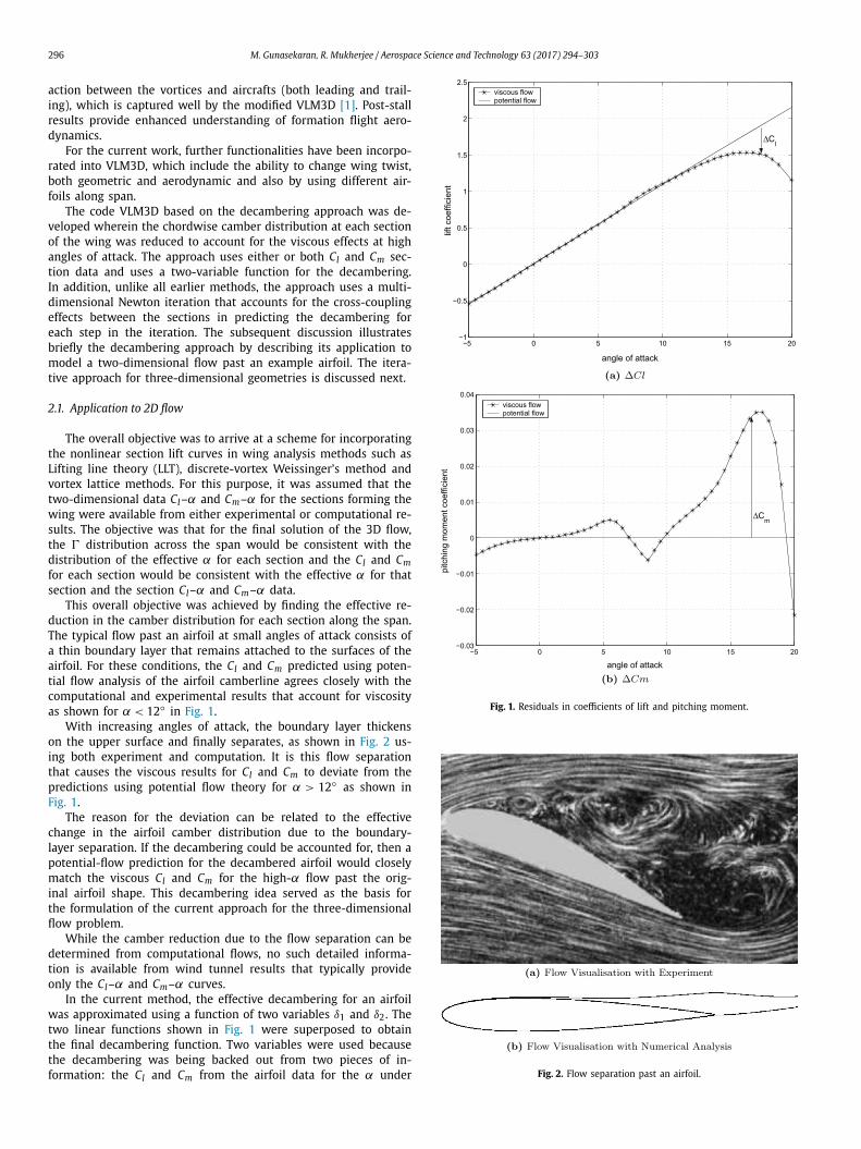
This overall objective was achieved by finding the effective re-duction in the camber distribution for each section along the span. The typical flow past an airfoil at small angles of attack consists of a thin boundary layer that remains attached to the surfaces of the airfoil. For these conditions, the Cl and Cm predicted using poten-tial flow analysis of the airfoil camberline agrees closely with the computational and experimental results that account for viscosity as shown for α < 12◦ in Fig. 1.

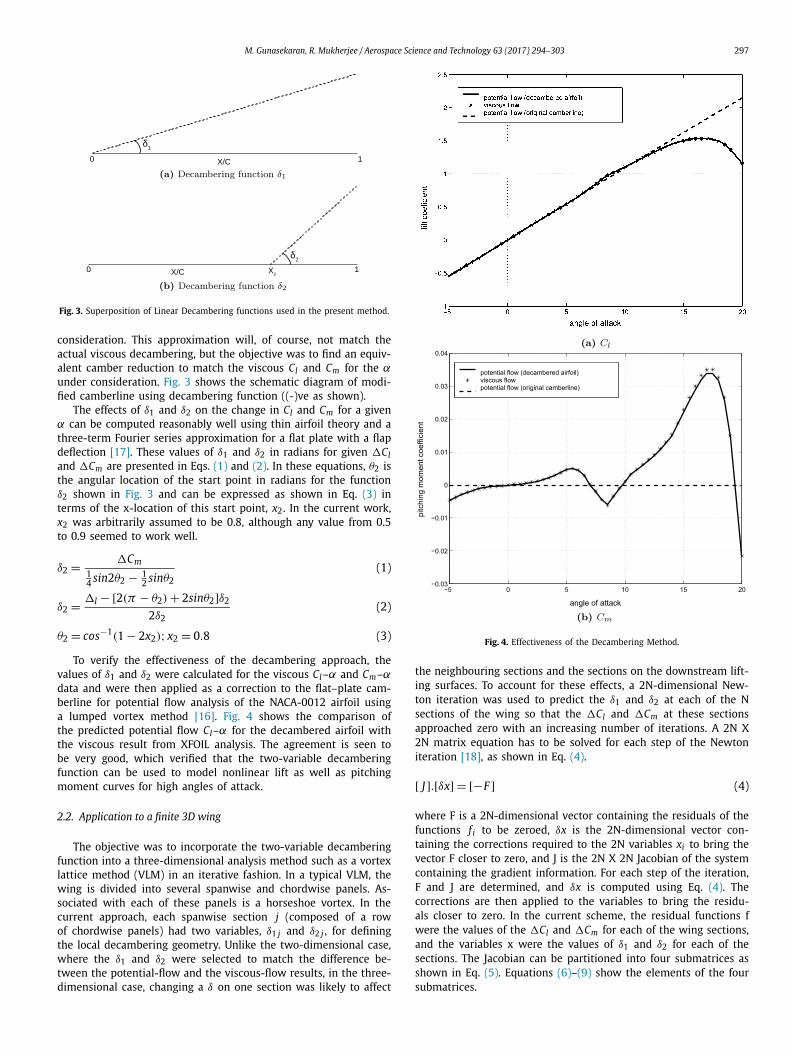
With increasing angles of attack, the boundary layer thickens on the upper surface and finally separates, as shown in Fig. 2 us-ing both experiment and computation. It is this flow separation that causes the viscous results for Cl and Cm to deviate from the predictions using potential flow theory for α > 12◦ as shown in Fig. 1.

The reason for the deviation can be related to the effective change in the airfoil camber distribution due to the boundary-layer separation. If the decambering could be accounted for, then a potential-flow prediction for the decambered airfoil would closely match the viscous Cl and Cm for the high-α flow past the orig-inal airfoil shape. This decambering idea served as the basis for the formulation of the current approach for the three-dimensional flow problem.

While the camber reduction due to the flow separation can be determined from computational flows, no such detailed informa-tion is available from wind tunnel results that typically provide only the Cl–α and Cm–α curves.

In the current method, the effective decambering for an airfoil was approximated using a function of two variables δ1 and δ2. The two linear functions shown in Fig. 1 were superposed to obtain the final decambering function. Two variables were used because the decambering was being backed out from two pieces of in-formation: the Cl and Cm from the airfoil data for the α under

Fig. 1. Residuals in coefficients of lift and pitching moment.

Fig. 2. Flow separation past an airfoil.

M. Gunasekaran, R. Mukherjee / Aerospace Science and Technology 63 (2017) 294–303 297

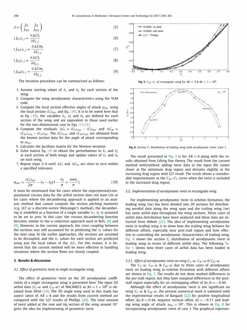
Fig. 3. Superposition of Linear Decambering functions used in the present method.

consideration. This approximation will, of course, not match the actual viscous decambering, but the objective was to find an equiv-alent camber reduction to match the viscous Cl and Cm for the αunder consideration. Fig. 3 shows the schematic diagram of modi-fied camberline using decambering function ((-)ve as shown).

The effects of δ1 and δ2 on the change in Cl and Cm for a given α can be computed reasonably well using thin airfoil theory and a three-term Fourier series approximation for a flat plate with a flap deflection [17]. These values of δ1 and δ2 in radians for given �Cland �Cm are presented in Eqs. (1) and (2). In these equations, θ2 is the angular location of the start point in radians for the function δ2 shown in Fig. 3 and can be expressed as shown in Eq. (3) in terms of the x-location of this start point, x2. In the current work, x2 was arbitrarily assumed to be 0.8, although any value from 0.5 to 0.9 seemed to work well.

δ2 = �Cm14 sin2θ2 − 1

2 sinθ2(1)

δ2 = �l − [2(π − θ2) + 2sinθ2]δ2

2δ2(2)

θ2 = cos−1(1 − 2x2); x2 = 0.8 (3)

To verify the effectiveness of the decambering approach, the values of δ1 and δ2 were calculated for the viscous Cl–α and Cm–αdata and were then applied as a correction to the flat–plate cam-berline for potential flow analysis of the NACA-0012 airfoil using a lumped vortex method [16]. Fig. 4 shows the comparison of the predicted potential flow Cl–α for the decambered airfoil with the viscous result from XFOIL analysis. The agreement is seen to be very good, which verified that the two-variable decambering function can be used to model nonlinear lift as well as pitching moment curves for high angles of attack.

2.2. Application to a finite 3D wing

The objective was to incorporate the two-variable decambering function into a three-dimensional analysis method such as a vortex lattice method (VLM) in an iterative fashion. In a typical VLM, the wing is divided into several spanwise and chordwise panels. As-sociated with each of these panels is a horseshoe vortex. In the current approach, each spanwise section j (composed of a row of chordwise panels) had two variables, δ1 j and δ2 j , for defining the local decambering geometry. Unlike the two-dimensional case, where the δ1 and δ2 were selected to match the difference be-tween the potential-flow and the viscous-flow results, in the three-dimensional case, changing a δ on one section was likely to affect

Fig. 4. Effectiveness of the Decambering Method.

the neighbouring sections and the sections on the downstream lift-ing surfaces. To account for these effects, a 2N-dimensional New-ton iteration was used to predict the δ1 and δ2 at each of the N sections of the wing so that the �Cl and �Cm at these sections approached zero with an increasing number of iterations. A 2N X 2N matrix equation has to be solved for each step of the Newton iteration [18], as shown in Eq. (4).

[ J ].[δx] = [−F ] (4)

where F is a 2N-dimensional vector containing the residuals of the functions f i to be zeroed, δx is the 2N-dimensional vector con-taining the corrections required to the 2N variables xi to bring the vector F closer to zero, and J is the 2N X 2N Jacobian of the system containing the gradient information. For each step of the iteration, F and J are determined, and δx is computed using Eq. (4). The corrections are then applied to the variables to bring the residu-als closer to zero. In the current scheme, the residual functions f were the values of the �Cl and �Cm for each of the wing sections, and the variables x were the values of δ1 and δ2 for each of the sections. The Jacobian can be partitioned into four submatrices as shown in Eq. (5). Equations (6)–(9) show the elements of the four submatrices.

298 M. Gunasekaran, R. Mukherjee / Aerospace Science and Technology 63 (2017) 294–303

J =(

Jl1 Jl2Jm1 Jm2

)(5)

( Jl1)i, j = ∂�Cli

∂δ1, j(6)

( Jm1)i, j = ∂�Cmi

∂δ1, j(7)

( Jl2)i, j = ∂�Cli

∂δ2, j(8)

( Jm2)i, j = ∂�Cmi

∂δ2, j(9)

The iteration procedure can be summarized as follows:

1. Assume starting values of δ1 and δ2 for each section of the wing.

2. Compute the wing aerodynamic characteristics using the VLM code.

3. Compute the local section effective angles of attack αsec using the local section (Cl)sec and Eq. (10). It is to be noted here that in Eq. (10), the variables δ1, δ2 and θ2 are defined for each section of the wing and are equivalent to those used earlier for the two-dimensional case in Eqs. (1)–(3).

4. Compute the residuals �Cl = (Cl)visc − (Cl)sec and �Cm =(Cm)visc − (Cm)sec . The (Cl)visc and (Cm)visc are obtained from the known section data for the angle of attack corresponding to αsec .

5. Calculate the Jacobian matrix for the Newton iteration.6. Solve matrix Eq. (4) to obtain the perturbations to δ1 and δ2

at each section of both wings and update values of δ1 and δ2on each wing.

7. Repeat steps 2–6 until �Cl and �Cm are close to zero within a specified tolerance.

αsec = (Cl)sec

2π− δ1 − δ2[1 − θ2

π+ sinθ2

π] (10)

It must be mentioned that for cases where the experimental/com-putational viscous data for the airfoil section does not have Cm or for cases where the decambering approach is applied to an anal-ysis method that cannot compute the section pitching moments (e.g. LLT or a discrete-vortex Weissinger’s method), the decamber-ing is modelled as a function of a single variable δ1; δ2 is assumed to be set to zero. In this case, the viscous decambering function becomes similar to the α-reduction approach used in Refs. [8] and [9]. However, in the current approach, the cross coupling between the sections was still accounted for in predicting the δ1 values for the next step. In the earlier approaches, the sections are assumed to be decoupled, and the δ1 values for each section are predicted using just the local values of the �Cl . For this reason, it is be-lieved that the current method will be more effective in handling situations where the section flows are closely coupled.

3. Results & discussion

3.1. Effect of geometric twist in single rectangular wing

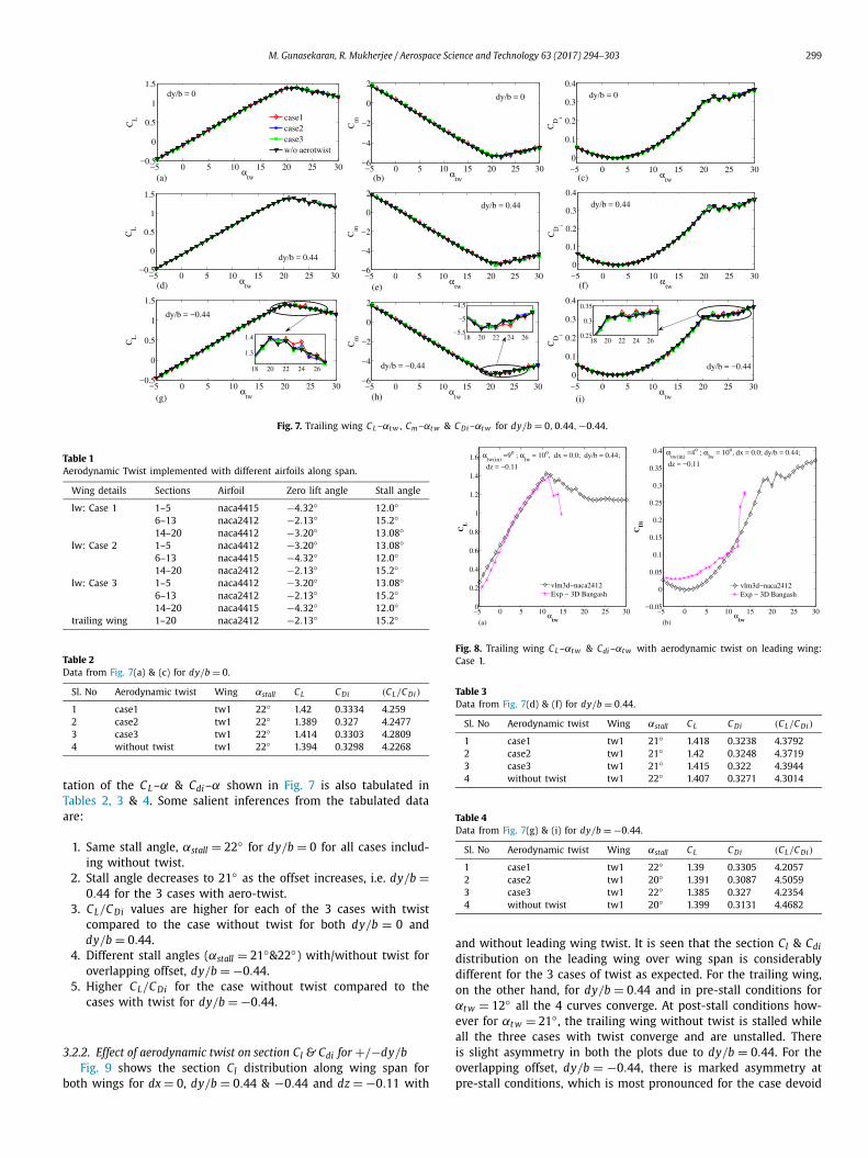
The effect of geometric twist on the 3D aerodynamic coeffi-cients of a single rectangular wing is presented here. The input 2D airfoil data (Cl–α and Cm–α) of NACA0012 at Re = 1 × 106 is ob-tained from XFoil [19]. The 3D single wing used in this study has aspect ratios of AR = 4 and the results from current method are compared with the LLT results of Phillips [20]. The total amount of twist added at the root and tip section of the wing around 10◦gives the idea for implementing of geometric twist.

Fig. 5. C Di –CL of rectangular wing for AR = 4 & Re = 1 × 106.

Fig. 6. Section Cl distribution of leading wing with aerodynamic twist: Case 1.

The result presented in Fig. 5 is for AR = 4 along with the re-sults obtained from Lifting line theory. The result from the current method with/without adding twist data in the input file comes closer at the minimum drag region and deviates slightly in the increasing drag region with LLT result. The result shows a consider-able improvements in the C Di –CL curve when the twist is included in the increased drag region.

3.2. Implementation of aerodynamic twist in rectangular wing

For implementing aerodynamic twist in echelon formation, the leading wing (lw) has been divided into 20 sections for distribut-ing aerofoil data along the wing span and the trailing wing (tw) has same airfoil data throughout the wing sections. Three cases of airfoil data distribution have been analyzed and these data are ex-tracted from Abbott [21]. The idea of implementing aerodynamic twist in leading wing is to show how the trailing wing behaves for different offsets, especially near post-stall region and how effec-tive in controlling the aerodynamic characteristics of trailing wing. Fig. 6 shows the section Cl distribution of aerodynamic twist in leading wing in terms of different airfoil data. The following Ta-ble 1 shows how three cases of airfoil data has been loaded in leading wing.

3.2.1. Effect of aerodynamic twist on wing CL–α, Cm–α & Cdi –αThe CL –α, Cm–α & Cdi –α due to three cases of aerodynamic

twist on leading wing in echelon formation with different offsets are shown in Fig. 7. The results do not show marked differences in the pre-stall region, but they have marginal differences in the post-stall region especially for an overlapping offset of dy/b = −0.44.

Although the effect of aerodynamic twist is not significant on wing CL –α & Cdi –α, the present numerical work is validated with the experimental results of Bangash [22] for positive longitudinal offset, dy/b = 0.44, negative vertical offset, dz = −0.11 and lead-ing wing angle of attack, αlw = 10◦ . This is shown in Fig. 8 for incorporating aerodynamic twist of case 1. The graphical represen-

M. Gunasekaran, R. Mukherjee / Aerospace Science and Technology 63 (2017) 294–303 299

Fig. 7. Trailing wing CL –αt w , Cm–αt w & C Di –αt w for dy/b = 0,0.44,−0.44.

Table 1Aerodynamic Twist implemented with different airfoils along span.

Wing details Sections Airfoil Zero lift angle Stall angle

lw: Case 1 1–5 naca4415 −4.32◦ 12.0◦6–13 naca2412 −2.13◦ 15.2◦14–20 naca4412 −3.20◦ 13.08◦

lw: Case 2 1–5 naca4412 −3.20◦ 13.08◦6–13 naca4415 −4.32◦ 12.0◦14–20 naca2412 −2.13◦ 15.2◦

lw: Case 3 1–5 naca4412 −3.20◦ 13.08◦6–13 naca2412 −2.13◦ 15.2◦14–20 naca4415 −4.32◦ 12.0◦

trailing wing 1–20 naca2412 −2.13◦ 15.2◦

Table 2Data from Fig. 7(a) & (c) for dy/b = 0.

Sl. No Aerodynamic twist Wing αstall CL C Di (CL/C Di)

1 case1 tw1 22◦ 1.42 0.3334 4.2592 case2 tw1 22◦ 1.389 0.327 4.24773 case3 tw1 22◦ 1.414 0.3303 4.28094 without twist tw1 22◦ 1.394 0.3298 4.2268

tation of the CL –α & Cdi –α shown in Fig. 7 is also tabulated in Tables 2, 3 & 4. Some salient inferences from the tabulated data are:

1. Same stall angle, αstall = 22◦ for dy/b = 0 for all cases includ-ing without twist.

2. Stall angle decreases to 21◦ as the offset increases, i.e. dy/b =0.44 for the 3 cases with aero-twist.

3. CL/C Di values are higher for each of the 3 cases with twist compared to the case without twist for both dy/b = 0 and dy/b = 0.44.

4. Different stall angles (αstall = 21◦&22◦) with/without twist for overlapping offset, dy/b = −0.44.

5. Higher CL/C Di for the case without twist compared to the cases with twist for dy/b = −0.44.

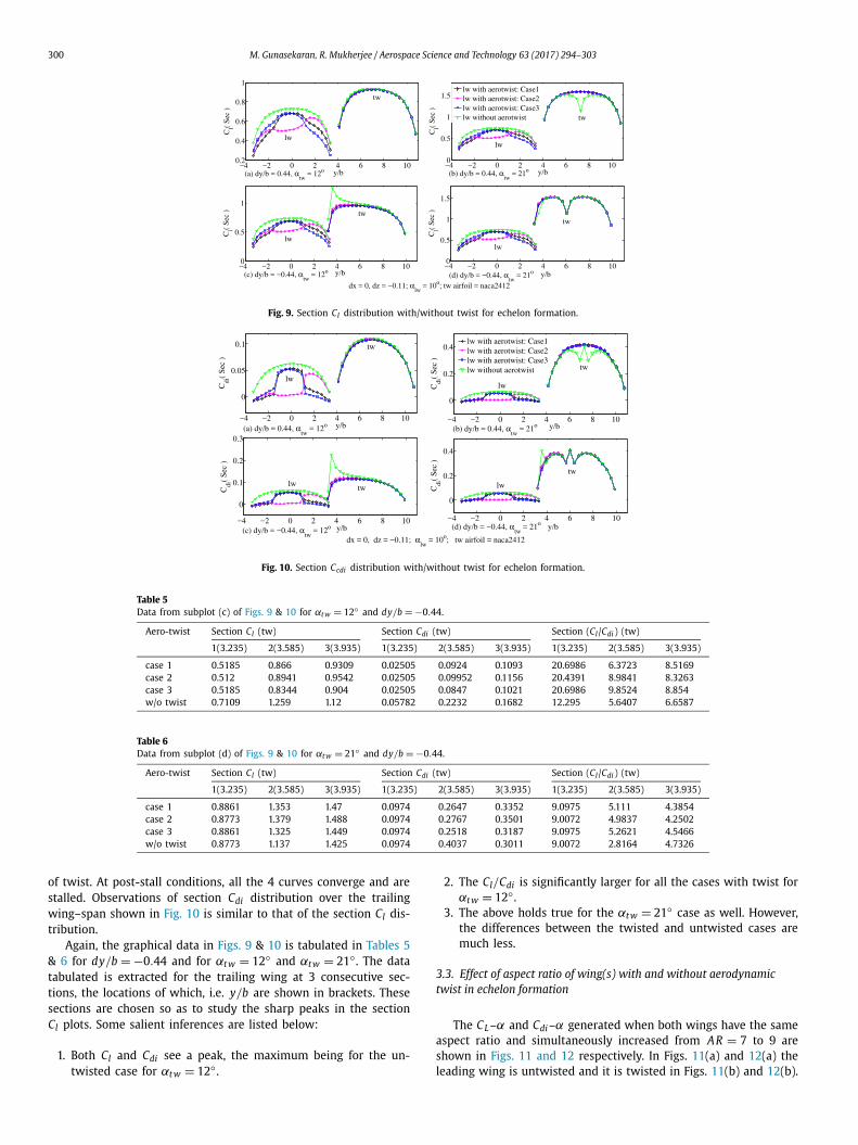
3.2.2. Effect of aerodynamic twist on section Cl & Cdi for +/−dy/bFig. 9 shows the section Cl distribution along wing span for

both wings for dx = 0, dy/b = 0.44 & −0.44 and dz = −0.11 with

Fig. 8. Trailing wing CL –αt w & Cdi –αt w with aerodynamic twist on leading wing: Case 1.

Table 3Data from Fig. 7(d) & (f) for dy/b = 0.44.

Sl. No Aerodynamic twist Wing αstall CL C Di (CL/C Di)

1 case1 tw1 21◦ 1.418 0.3238 4.37922 case2 tw1 21◦ 1.42 0.3248 4.37193 case3 tw1 21◦ 1.415 0.322 4.39444 without twist tw1 22◦ 1.407 0.3271 4.3014

Table 4Data from Fig. 7(g) & (i) for dy/b = −0.44.

Sl. No Aerodynamic twist Wing αstall CL C Di (CL/C Di)

1 case1 tw1 22◦ 1.39 0.3305 4.20572 case2 tw1 20◦ 1.391 0.3087 4.50593 case3 tw1 22◦ 1.385 0.327 4.23544 without twist tw1 20◦ 1.399 0.3131 4.4682

and without leading wing twist. It is seen that the section Cl & Cdi

distribution on the leading wing over wing span is considerably different for the 3 cases of twist as expected. For the trailing wing, on the other hand, for dy/b = 0.44 and in pre-stall conditions for αt w = 12◦ all the 4 curves converge. At post-stall conditions how-ever for αt w = 21◦ , the trailing wing without twist is stalled while all the three cases with twist converge and are unstalled. There is slight asymmetry in both the plots due to dy/b = 0.44. For the overlapping offset, dy/b = −0.44, there is marked asymmetry at pre-stall conditions, which is most pronounced for the case devoid

300 M. Gunasekaran, R. Mukherjee / Aerospace Science and Technology 63 (2017) 294–303

Fig. 9. Section Cl distribution with/without twist for echelon formation.

Fig. 10. Section Ccdi distribution with/without twist for echelon formation.

Table 5Data from subplot (c) of Figs. 9 & 10 for αt w = 12◦ and dy/b = −0.44.

Aero-twist Section Cl (tw) Section Cdi (tw) Section (Cl/Cdi ) (tw)

1(3.235) 2(3.585) 3(3.935) 1(3.235) 2(3.585) 3(3.935) 1(3.235) 2(3.585) 3(3.935)

case 1 0.5185 0.866 0.9309 0.02505 0.0924 0.1093 20.6986 6.3723 8.5169case 2 0.512 0.8941 0.9542 0.02505 0.09952 0.1156 20.4391 8.9841 8.3263case 3 0.5185 0.8344 0.904 0.02505 0.0847 0.1021 20.6986 9.8524 8.854w/o twist 0.7109 1.259 1.12 0.05782 0.2232 0.1682 12.295 5.6407 6.6587

Table 6Data from subplot (d) of Figs. 9 & 10 for αt w = 21◦ and dy/b = −0.44.

Aero-twist Section Cl (tw) Section Cdi (tw) Section (Cl/Cdi ) (tw)

1(3.235) 2(3.585) 3(3.935) 1(3.235) 2(3.585) 3(3.935) 1(3.235) 2(3.585) 3(3.935)

case 1 0.8861 1.353 1.47 0.0974 0.2647 0.3352 9.0975 5.111 4.3854case 2 0.8773 1.379 1.488 0.0974 0.2767 0.3501 9.0072 4.9837 4.2502case 3 0.8861 1.325 1.449 0.0974 0.2518 0.3187 9.0975 5.2621 4.5466w/o twist 0.8773 1.137 1.425 0.0974 0.4037 0.3011 9.0072 2.8164 4.7326

of twist. At post-stall conditions, all the 4 curves converge and are stalled. Observations of section Cdi distribution over the trailing wing–span shown in Fig. 10 is similar to that of the section Cl dis-tribution.

Again, the graphical data in Figs. 9 & 10 is tabulated in Tables 5& 6 for dy/b = −0.44 and for αt w = 12◦ and αt w = 21◦ . The data tabulated is extracted for the trailing wing at 3 consecutive sec-tions, the locations of which, i.e. y/b are shown in brackets. These sections are chosen so as to study the sharp peaks in the section Cl plots. Some salient inferences are listed below:

1. Both Cl and Cdi see a peak, the maximum being for the un-twisted case for αt w = 12◦ .

2. The Cl/Cdi is significantly larger for all the cases with twist for αt w = 12◦ .

3. The above holds true for the αt w = 21◦ case as well. However, the differences between the twisted and untwisted cases are much less.

3.3. Effect of aspect ratio of wing(s) with and without aerodynamic twist in echelon formation

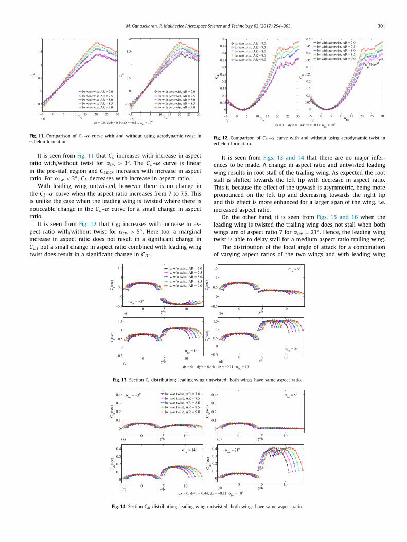
The CL –α and Cdi –α generated when both wings have the same aspect ratio and simultaneously increased from AR = 7 to 9 are shown in Figs. 11 and 12 respectively. In Figs. 11(a) and 12(a) the leading wing is untwisted and it is twisted in Figs. 11(b) and 12(b).

M. Gunasekaran, R. Mukherjee / Aerospace Science and Technology 63 (2017) 294–303 301

Fig. 11. Comparison of CL –α curve with and without using aerodynamic twist in echelon formation.

It is seen from Fig. 11 that CL increases with increase in aspect ratio with/without twist for αt w > 3◦ . The CL –α curve is linear in the pre-stall region and CLmax increases with increase in aspect ratio. For αt w < 3◦ , CL decreases with increase in aspect ratio.

With leading wing untwisted, however there is no change in the CL –α curve when the aspect ratio increases from 7 to 7.5. This is unlike the case when the leading wing is twisted where there is noticeable change in the CL –α curve for a small change in aspect ratio.

It is seen from Fig. 12 that C Di increases with increase in as-pect ratio with/without twist for αt w > 5◦ . Here too, a marginal increase in aspect ratio does not result in a significant change in C Di but a small change in aspect ratio combined with leading wing twist does result in a significant change in C Di .

Fig. 12. Comparison of Cdi –α curve with and without using aerodynamic twist in echelon formation.

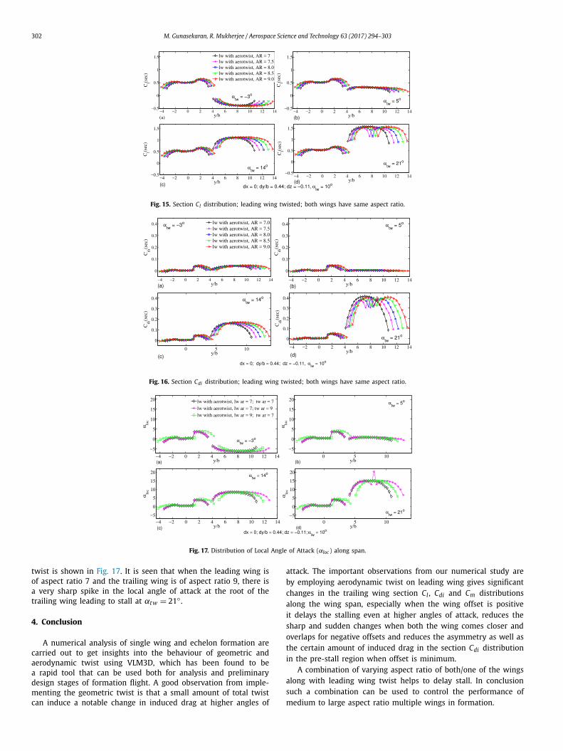
It is seen from Figs. 13 and 14 that there are no major infer-ences to be made. A change in aspect ratio and untwisted leading wing results in root stall of the trailing wing. As expected the root stall is shifted towards the left tip with decrease in aspect ratio. This is because the effect of the upwash is asymmetric, being more pronounced on the left tip and decreasing towards the right tip and this effect is more enhanced for a larger span of the wing. i.e. increased aspect ratio.

On the other hand, it is seen from Figs. 15 and 16 when the leading wing is twisted the trailing wing does not stall when both wings are of aspect ratio 7 for αt w = 21◦ . Hence, the leading wing twist is able to delay stall for a medium aspect ratio trailing wing.

The distribution of the local angle of attack for a combination of varying aspect ratios of the two wings and with leading wing

Fig. 13. Section Cl distribution; leading wing untwisted; both wings have same aspect ratio.

Fig. 14. Section Cdi distribution; leading wing untwisted; both wings have same aspect ratio.

302 M. Gunasekaran, R. Mukherjee / Aerospace Science and Technology 63 (2017) 294–303

Fig. 15. Section Cl distribution; leading wing twisted; both wings have same aspect ratio.

Fig. 16. Section Cdi distribution; leading wing twisted; both wings have same aspect ratio.

Fig. 17. Distribution of Local Angle of Attack (αloc ) along span.

twist is shown in Fig. 17. It is seen that when the leading wing is of aspect ratio 7 and the trailing wing is of aspect ratio 9, there is a very sharp spike in the local angle of attack at the root of the trailing wing leading to stall at αt w = 21◦ .

4. Conclusion

A numerical analysis of single wing and echelon formation are carried out to get insights into the behaviour of geometric and aerodynamic twist using VLM3D, which has been found to be a rapid tool that can be used both for analysis and preliminary design stages of formation flight. A good observation from imple-menting the geometric twist is that a small amount of total twist can induce a notable change in induced drag at higher angles of

attack. The important observations from our numerical study are by employing aerodynamic twist on leading wing gives significant changes in the trailing wing section Cl , Cdi and Cm distributions along the wing span, especially when the wing offset is positive it delays the stalling even at higher angles of attack, reduces the sharp and sudden changes when both the wing comes closer and overlaps for negative offsets and reduces the asymmetry as well as the certain amount of induced drag in the section Cdi distribution in the pre-stall region when offset is minimum.

A combination of varying aspect ratio of both/one of the wings along with leading wing twist helps to delay stall. In conclusion such a combination can be used to control the performance of medium to large aspect ratio multiple wings in formation.

M. Gunasekaran, R. Mukherjee / Aerospace Science and Technology 63 (2017) 294–303 303

Conflict of interest statement

We have no conflict of interest to declare.

References

[1] M. Gunasekaran, Rinku Mukherjee, A Numerical Study of the Aerodynamics of Cessna 172 Aircrafts in Echelon Formation, AIAA 2014-1107.

[2] C. Wiselsberger, Beitrag zur Erklarung des Winkelfluges eineger Zugvogel, ZFM, Z. Flugtech. Mot.luftschiffahrt 5 (1914) 225–229.

[3] H. Schlichting, Leistungsersparnis in Verbandsflug, Ber. Aerodyn. Inst. T. H. Braunschw. 42 (6) (1942).

[4] D. Hummel, Recent Aerodynamic Contributions to Problems of Birds Flight, ICAS1978/A 1-05.

[5] Markus Beukenberg, Dietrich Hummel, Aerodynamics, Performance and Control of Airplanes in Formation Flight, ICAS-90-5.9.3.

[6] W.F. Phillips, Mechanics of Flight, 2nd edition, John Wiley & Sons, United King-dom, October 2009, Chapter 1.

[7] P.J. Boschetti, A. Amerio, E.M. Cárdenas, Aerodynamic Performance as a Func-tion of Local Twist in an Unmanned Airplane, AIAA paper 2009-1481, January 2009.

[8] Lingxiao Zheng, Tyson L. Hedrick, Rajat Mittal, Time-varying wing–twist im-proves aerodynamic efficiency of forward flight in butterflies, PLoS ONE 8 (1) (January 2013) e53060.

[9] Geoffrey C. Bower, Tristan C. Flanzer, Ilan M. Kroo, Formation Geometries and Route Optimization for Commercial Formation, Flight, AIAA 2009-3615.

[10] Ashok Gopalarathnam, Aerodynamic Benefit of Aircraft Formation Flight, Ency-clopedia of Aerospace Engineering, John Wiley & Sons, Ltd, 2010.

[11] H.P. Thien, M.A. Moelyadi, H. Muhammad, Effects of Leader’s Position and Shape on Aerodynamic Performances of V Flight Formation, ICIUS2007-A008.

[12] Sara Nichols, Liamm Skerritt, Thomas Bee, Structural analysis of composite aerofoils using aero- and inertial-elastic tailoring, Struct. Dyn. 1 (October 2010) 57–67.

[13] Kevin A. Lane, David D. Marshall, Rob A. McDonald, Lift Superposition and Aerodynamic Twist Optimization for Achieving Desired Lift Distributions, AIAA 2010-1227.

[14] Vanessa L. Bond, Robert A. Canfield, Maria da Luz Madruga Santos Matos, Afzal Suleman, Maxwell Blair, Joined-wing wind-tunnel test for longitudinal control via aftwing twist, J. Aircr. 47 (5) (2010) 1481–1489.

[15] Ivan Korkischko, Robert Konrath, Formation flight of low-aspect-ratio wings at low Reynolds number, J. Aircr. (2016), http://dx.doi.org/10.2514/1.C033941, in press.

[16] R. Mukherjee, A. Gopalarathnam, Post-stall prediction of multiple-lifting-surface configurations using a decambering approach, J. Aircr. 43 (3) (May–June 2006) 660–668.

[17] J. Katz, A. Plotkin, Low-Speed Aerodynamics from Wing Theory to Panel Meth-ods, McGraw–Hill, Inc., 1991.

[18] W.H. Press, S.A. Teukolsky, W.T. Vetterling, B.P. Flannery, Numerical Recipes in Fortran – The Art of Scientific Computing, 2nd ed., Cambridge University Press, New York, 1992.

[19] M. Drela, XFOIL: an analysis and design system for low Reynolds number air-foils, low Reynolds number aerodynamics, in: T.J. Mueller (Ed.), Lect. Notes Eng., vol. 54, Springer-Verlag, New York, June 1989, pp. 1–12.

[20] W.F. Phillips, Lifting-line analysis for twisted wings and washout-optimized wings, J. Aircr. 41 (1) (2004) 128–136.

[21] Ira H. Abbott, Albert E. Von Doenhoff, Theory of Wing Sections, Dover, Mineola, NY, 1959.

[22] Z.A. Bangash, R.P. Sanchez, A. Ahmed, Aerodynamics of formation flight, J. Aircr. 43 (4) (July–August 2006) 907–912.