Advances in Water Resources 106 (2017) 80–94

Contents lists available at ScienceDirect

Advances in Water Resources

journal homepage: www.elsevier.com/locate/advwatres

Anomalous transport in disordered fracture networks: Spatial Markov

model for dispersion with variable injection modes

Peter K. Kang

a , b , ∗, Marco Dentz

c , Tanguy Le Borgne

d , Seunghak Lee

a , Ruben Juanes b

a Korea Institute of Science and Technology, Seoul 02792, Republic of Korea b Massachusetts Institute of Technology, 77 Massachusetts Ave, Building 1, Cambridge, Massachusetts 02139, USA c Institute of Environmental Assessment and Water Research (IDÆA), Spanish National Research Council (CSIC), 08034 Barcelona, Spain d Université de Rennes 1, CNRS, Geosciences Rennes, UMR 6118, Rennes, France

a r t i c l e i n f o

Article history:

Received 25 May 2016

Revised 24 March 2017

Accepted 31 March 2017

Available online 3 April 2017

Keywords:

Discrete fracture networks

Injection modes

Anomalous transport

Stochastic modeling

Lagrangian velocity

Time domain random walks

Continuous time random walks

Spatial Markov model

a b s t r a c t

We investigate tracer transport on random discrete fracture networks that are characterized by the statis-

tics of the fracture geometry and hydraulic conductivity. While it is well known that tracer transport

through fractured media can be anomalous and particle injection modes can have major impact on dis-

persion, the incorporation of injection modes into effective transport modeling has remained an open

issue. The fundamental reason behind this challenge is that—even if the Eulerian fluid velocity is steady—

the Lagrangian velocity distribution experienced by tracer particles evolves with time from its initial dis-

tribution, which is dictated by the injection mode, to a stationary velocity distribution. We quantify this

evolution by a Markov model for particle velocities that are equidistantly sampled along trajectories. This

stochastic approach allows for the systematic incorporation of the initial velocity distribution and quanti-

fies the interplay between velocity distribution and spatial and temporal correlation. The proposed spatial

Markov model is characterized by the initial velocity distribution, which is determined by the particle in-

jection mode, the stationary Lagrangian velocity distribution, which is derived from the Eulerian velocity

distribution, and the spatial velocity correlation length, which is related to the characteristic fracture

length. This effective model leads to a time-domain random walk for the evolution of particle positions

and velocities, whose joint distribution follows a Boltzmann equation. Finally, we demonstrate that the

proposed model can successfully predict anomalous transport through discrete fracture networks with

different levels of heterogeneity and arbitrary tracer injection modes.

© 2017 Elsevier Ltd. All rights reserved.

e

s

a

b

t

b

f

m

t

i

e

G

1

t

t

1. Introduction

Flow and transport in fractured geologic media control many

important natural and engineered processes, including nuclear

waste disposal, geologic carbon sequestration, groundwater con-

tamination, managed aquifer recharge, and geothermal production

in fractured geologic media (e.g., Bodvarsson et al., 1999; Lewicki

et al., 2007; Tang et al., 1981; Chrysikopoulos et al., 2009; Pruess,

2006 ). Two dominant approaches exist for simulating flow and

transport through fractured media: the equivalent porous medium

approach ( Neuman et al., 1987; Tsang et al., 1996 ) and the discrete

fracture network approach (DFN) ( Bernabe et al., 2016; Cacas et al.,

1990; de Dreuzy et al., 2012; Frampton and Cvetkovic, 2011; Hy-

man et al., 2015a; Juanes et al., 2002; Karimi-Fard et al., 2004; Ki-

raly, 1979; Makedonska et al., 2015; Martinez-Landa and Carrera,

2005; Moreno and Neretnieks, 1993; Nordqvist et al., 1992; Park

∗ Corresponding author.

E-mail address: pkkang@kist.re.kr (P.K. Kang).

p

m

t

http://dx.doi.org/10.1016/j.advwatres.2017.03.024

0309-1708/© 2017 Elsevier Ltd. All rights reserved.

t al., 2003; Schmid et al., 2013 ). The DFN approach explicitly re-

olves individual fractures whereas the equivalent porous medium

pproach represents the fractured medium as a single continuum

y deriving effective parameters to include the effect of the frac-

ures on the flow and transport. The latter, however, is hampered

y the fact that a representative elementary volume may not exist

or fractured media ( Bear, 1972; de Marsily, 1986 ). Dual-porosity

odels are in between these two approaches, and conceptualize

he fractured-porous medium as two overlapping continua, which

nteract via an exchange term ( Arbogast et al., 1990; Barenblatt

t al., 1960; Bibby, 1981; Feenstra et al., 1985; Gerke and van

enuchten, 1993; Kazemi et al., 1976; Maloszewski and Zuber,

985; Pruess, 1985; Warren and Root, 1963 ).

DFN modeling has advanced significantly in recent years with

he increase in computational power. Current DFN simulators can

ake into account multiple physical mechanisms occurring in com-

lex 3D fracture systems. Recent studies also have developed

ethods to explicitly model advection and diffusion through both

he discrete fractures and the permeable rock matrix ( Geiger et al.,

P.K. Kang et al. / Advances in Water Resources 106 (2017) 80–94 81

2

m

c

t

2

t

t

e

i

i

p

d

(

u

s

s

b

p

e

g

2

2

2

2

e

t

w

K

a

d

t

r

m

t

d

e

a

h

m

p

P

s

i

e

i

e

D

L

s

fl

d

t

b

2

2

a

o

t

t

v

c

f

D

p

2

J

2

m

w

C

o

t

m

t

t

D

j

r

r

a

c

b

w

d

a

d

t

t

p

I

b

S

g

k

S

i

t

a

i

t

v

b

t

I

2

2

r

t

t

2

e

w

e

p

d

d

t

d

fi

c

f

010; Houseworth et al., 2013; Sebben and Werner, 2016; Will-

ann et al., 2013 ). In practice, however, their application must ac-

ount for the uncertainty in the subsurface characterization of frac-

ured media, which is still an considerable challenge ( Chen et al.,

006; Dorn et al., 2012; Kang et al., 2016b ). Thus, there is a con-

inued interest in the development of upscaled transport models

hat can be parameterized with a small number of model param-

ters. Ideally, these model parameters should have a clear physical

nterpretation and should be determined by means of field exper-

ments, with the expectation that the model can then be used for

redictive purposes ( Becker and Shapiro, 2003; Kang et al., 2015b ).

Developing an upscaled model for transport in fractured me-

ia is especially challenging due to the emergence of anomalous

non-Fickian) transport. While particle spreading is often described

sing a Fickian framework, anomalous transport—characterized by

cale-dependent spreading, early arrivals, long tails, and nonlinear

caling with time of the centered mean square displacement—has

een widely observed in porous and fractured media across multi-

le scales, from pore ( Bijeljic et al., 2011; Gjetvaj et al., 2015; Kang

t al., 2014; Scheven et al., 2005; Seymour et al., 2004 ) to sin-

le fracture ( Detwiler et al., 20 0 0; Drazer et al., 20 04; Kang et al.,

016a; Wang and Cardenas, 2014 ) to column ( Cortis and Berkowitz,

004; Hatano and Hatano, 1998 ) to field scale ( Becker and Shapiro,

0 0 0; Garabedian et al., 1991; Haggerty et al., 2001; Hyman et al.,

015b; Kang et al., 2015b; Le Borgne and Gouze, 2008; McKenna

t al., 2001 ). The ability to predict anomalous transport is essen-

ial because it leads to fundamentally different behavior compared

ith Fickian transport ( Bouchaud and Georges, 1990; Metzler and

lafter, 20 0 0; Shlesinger, 1974 ).

The continuous time random walk (CTRW) formalism ( Klafter

nd Silbey, 1980; Scher and Montroll, 1975 ) is a framework to

escribe anomalous transport through which models particle mo-

ion through a random walk in space and time characterized by

andom space and time increments, which accounts for variable

ass transfer rates due to spatial heterogeneity. It has been used

o model transport in heterogeneous porous and fractured me-

ia ( Berkowitz et al., 2006; Berkowitz and Scher, 1997; Dentz

t al., 2004; 2015; Geiger et al., 2010; Kang et al., 2011a; Wang

nd Cardenas, 2014 ) and allows incorporating information on flow

eterogeneity and medium geometry for large scale transport

odeling. Similarly, the time-domain random walk (TDRW) ap-

roach Benke and Painter (2003) ; Painter and Cvetkovic (2005) ;

ainter et al. (2008) models particle motion due to distributed

pace and time increments, which are derived from particle veloc-

ties and their correlations. The analysis of particle motion in het-

rogeneous flow fields demonstrate that Lagrangian particle veloc-

ties exhibit sustained correlation along their trajectory ( de Anna

t al., 2013; Benke and Painter, 2003; Cvetkovic et al., 1996;

atta et al., 2013; Gotovac et al., 2009; Kang et al., 2014; 2011b;

e Borgne et al., 2008; Meyer and Tchelepi, 2010 ). Volume con-

ervation induces correlation in the Eulerian velocity field because

uxes must satisfy the divergence-free constraint. This, in turn, in-

uces correlation in the Lagrangian velocity along a particle trajec-

ory. To take into account velocity correlation, Lagrangian models

ased on Markovian processes have been proposed ( de Anna et al.,

013; Benke and Painter, 2003; Kang et al., 2014; 2011b; 2015a;

015b; Le Borgne et al., 2008; Meyer and Tchelepi, 2010; Painter

nd Cvetkovic, 2005 ). Spatial Markov models are based on the

bservation that successive velocity transitions measured equidis-

antly along the mean flow direction exhibit Markovianity: a par-

icle’s velocity at the next step is fully determined by its current

elocity. The spatial Markov model, which accounts for velocity

orrelation by incorporating this one-step velocity correlation in-

ormation, has not yet been extended to disordered (unstructured)

FNs.

t

The mode of particle injection can have a major im-

act on transport through porous and fractured media ( Dagan,

016; Frampton and Cvetkovic, 2009; Hyman et al., 2015b;

ankovi c and Fiori, 2010; Kreft and Zuber, 1978; Le Borgne et al.,

010; 2007; Sposito and Dagan, 1994 ). Two generic injection

odes are uniform (resident) injection and flux-weighted injection

ith distinctive physical meanings as discussed in Frampton and

vetkovic (2009) . The work by Sposito and Dagan (1994) is one

f the earliest studies of the impact of different particle injec-

ion modes on the time evolution of a solute plume spatial mo-

ents. The significance of injection modes on particle transport

hrough discrete fracture networks has been studied for frac-

ured media ( Frampton and Cvetkovic, 2009; Hyman et al., 2015b ).

agan (2016) recently clarified the theoretical relation between in-

ection modes and plume mean velocity. Despite recent advances

egarding the significance of particle injection modes, the incorpo-

ation of injection methods into effective transport modeling is still

n open issue ( Frampton and Cvetkovic, 2009 ). The fundamental

hallenge is that the Lagrangian velocity distribution experienced

y tracer particles evolves with time from its initial distribution

hich is dictated by the injection mode to a stationary velocity

istribution ( Cvetkovic et al., 1996; Dentz et al., 2016; Frampton

nd Cvetkovic, 2009; Gotovac et al., 2009 ). In this paper, we ad-

ress these fundamental questions, in the context of anomalous

ransport through disordered DFNs.

The paper proceeds as follows. In the next section, we present

he studied random discrete fracture networks, the flow and trans-

ort equations and details of the different particle injection rules.

n Section 3 , we investigate the emergence of anomalous transport

y direct Monte Carlo simulations of flow and particle transport. In

ection 4 , we analyze Eulerian and Lagrangian velocity statistics to

ain insight into the effective particle dynamics and elucidate the

ey mechanisms that lead to the observed anomalous behavior. In

ection 5 , we develop a spatial Markov model that is character-

zed by the initial velocity distribution, probability density func-

ion (PDF) of Lagrangian velocities and their transition PDF, which

re derived from the Monte Carlo simulations. The proposed model

s in excellent agreement with direct Monte Carlo simulations. We

hen present a parsimonious spatial Markov model that quantifies

elocity correlation with a single parameter. The predictive capa-

ilities of this simplified model are demonstrated by comparison to

he direct Monte Carlo simulations with arbitrary injection modes.

n Section 6 , we summarize the main findings and conclusions.

. Flow and transport in discrete random fracture networks

.1. Random fracture networks

We numerically generate random DFNs in two-dimensional

ectangular regions, and solve for flow and tracer transport within

hese networks. The fracture networks are composed of linear frac-

ures embedded in an impermeable rock matrix. The idealized

D DFN realizations are generated by superimposing two differ-

nt sets of fractures, which leads to realistic discrete fracture net-

orks ( Geiger et al., 2010; Long et al., 1982 ). Fracture locations, ori-

ntations, lengths and hydraulic conductivities are generated from

redefined distributions, which are assumed to be statistically in-

ependent: (1) Fracture midpoints are selected randomly over the

omain size of L x × L y where L x = 2 and L y = 1 ; (2) Fracture orien-

ations for two fracture sets are selected randomly from Gaussian

istributions, with means and standard deviation of 0 ° ± 5 ° for the

rst set, and 90 ° ± 5 ° for the second set; (3) Fracture lengths are

hosen randomly from exponential distributions with mean L x /10

or the horizontal fracture set and mean L y /10 for the vertical frac-

ure set; (4) Fracture conductivities are assigned randomly from a

82 P.K. Kang et al. / Advances in Water Resources 106 (2017) 80–94

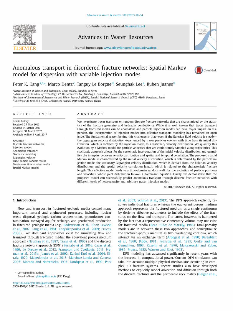
Fig. 1. (a) Example of a two-dimensional DFN studied here, with 20 0 0 fractures

(10 0 0 fractures for each fracture set). (b) Subsection of a spatially uncorrelated con-

ductivity field between 0 ≤ x ≤ 1 and 0.5 ≤ y ≤ 1. Conductivity values are assigned

from a lognormal distribution with σln K = 1 . Link width is proportional to the con-

ductivity value; only connected links are shown.

−

n

(

s

n

c

e

a

m

o

t

l

l

T

E

s

w

fl

P

E

m

t

h

T

v

a

m

fl

f

t

c

i

v

fl

o

2

t

j

m

U

o

c

N

w

t

t

i

N

U

c

a

l

predefined log-normal distribution. An example of a random dis-

crete fracture network with 20 0 0 fractures is shown in Fig. 1 .

The position vector of node i in the fracture network is denoted

by x i . The link length between nodes i and j is denoted by l ij . The

network is characterized by the distribution of link lengths p l ( l )

and hydraulic conductivity K . The PDF of link lengths here is ex-

ponential

p l (l) =

exp (−l/ l )

l . (1)

Note that the link length and orientation are independent. The

characteristic fracture link length is obtained by taking the average

of a link length over all the realizations, which gives l ≈ L x / 200 .

A realization of the random discrete fracture network is generated

by assigning independent and identically distributed random hy-

draulic conductivities K ij > 0 to each link between nodes i and j .

Therefore, the K ij values in different links are uncorrelated. The set

of all realizations of the spatially random network generated in this

way forms a statistical ensemble that is stationary and ergodic. We

assign a lognormal distribution of K values, and study the impact

of conductivity heterogeneity on transport by varying the variance

of ln ( K ). We study log-normal conductivity distributions with four

different variances: σln K = 1 , 2 , 3 , 5 . The use of this particular dis-

tribution is motivated by the fact that conductivity values in many

natural media can be described by a lognormal law ( Bianchi and

Snow, 1969; Sanchez-Vila et al., 2006 ).

2.2. Flow field

Steady state flow through the network is modeled by Darcy’s

law ( Bear, 1972 ) for the fluid flux u ij between nodes i and j , u i j =

K i j (� j − �i ) /l i j , where �i and �j are the hydraulic heads at

odes i and j . Imposing flux conservation at each node i , ∑

j u i j = 0

the summation is over nearest-neighbor nodes), leads to a linear

ystem of equations, which is solved for the hydraulic heads at the

odes. The fluid flux through a link from node i to j is termed in-

oming for node i if u ij < 0, and outgoing if u ij > 0. We denote by

ij the unit vector in the direction of the link connecting nodes i

nd j .

We study a uniform flow setting characterized by constant

ean flow in the positive x -direction parallel to the principal set

f factures. No-flow conditions are imposed at the top and bot-

om boundaries of the domain, and fixed hydraulic head at the

eft ( � = 1 ) and right ( � = 0 ) boundaries. The overbar in the fol-

owing denotes the ensemble average over all network realizations.

he one-point statistics of the flow field are characterized by the

ulerian velocity PDF, which is obtained by spatial and ensemble

ampling of the velocity magnitudes in the network

p e (u ) =

∑

i> j l i j δ(u − u i j )

N � l . (2)

here N � is the number of links in the network. Link length and

ow velocities here are independent. Thus, the Eulerian velocity

DF is given by

p e (u ) =

1

N �

∑

i> j

δ(u − u i j ) . (3)

ven though the underlying conductivity field is uncorrelated, the

ass conservation constraint together with heterogeneity leads to

he formation of preferential flow paths with increasing network

eterogeneity ( Bernabe and Bruderer, 1998; Kang et al., 2015a ).

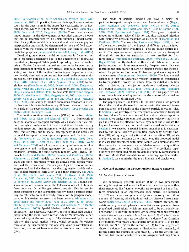
his is illustrated in Fig. 2 a and b, which show maps of the relative

elocity magnitude for high velocities in networks with log- K vari-

nces of 1 and 5. As shown in Fig. 2 c and d, for low heterogeneity

ost small flux values occur along links perpendicular to the mean

ow direction, whereas low flux values do not show directionality

or the high heterogeneity case. This indicates that fracture geome-

ry dominates small flux values for low heterogeneity and fracture

onductivity dominates small flux values for high heterogeneity. An

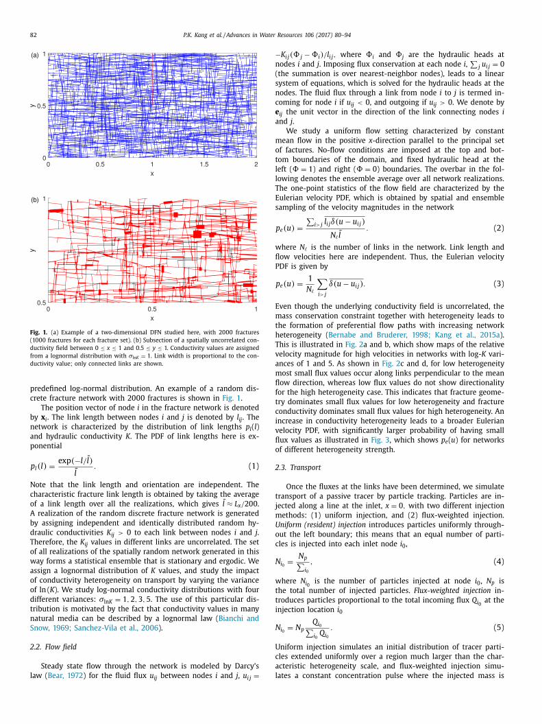
ncrease in conductivity heterogeneity leads to a broader Eulerian

elocity PDF, with significantly larger probability of having small

ux values as illustrated in Fig. 3 , which shows p e ( u ) for networks

f different heterogeneity strength.

.3. Transport

Once the fluxes at the links have been determined, we simulate

ransport of a passive tracer by particle tracking. Particles are in-

ected along a line at the inlet, x = 0 , with two different injection

ethods: (1) uniform injection, and (2) flux-weighted injection.

niform (resident) injection introduces particles uniformly through-

ut the left boundary; this means that an equal number of parti-

les is injected into each inlet node i 0 ,

i 0 =

N p ∑

i 0

, (4)

here N i 0 is the number of particles injected at node i 0 , N p is

he total number of injected particles. Flux-weighted injection in-

roduces particles proportional to the total incoming flux Q i 0 at the

njection location i 0

i 0 = N p

Q i 0 ∑

i 0 Q i 0

. (5)

niform injection simulates an initial distribution of tracer parti-

les extended uniformly over a region much larger than the char-

cteristic heterogeneity scale, and flux-weighted injection simu-

ates a constant concentration pulse where the injected mass is

P.K. Kang et al. / Advances in Water Resources 106 (2017) 80–94 83

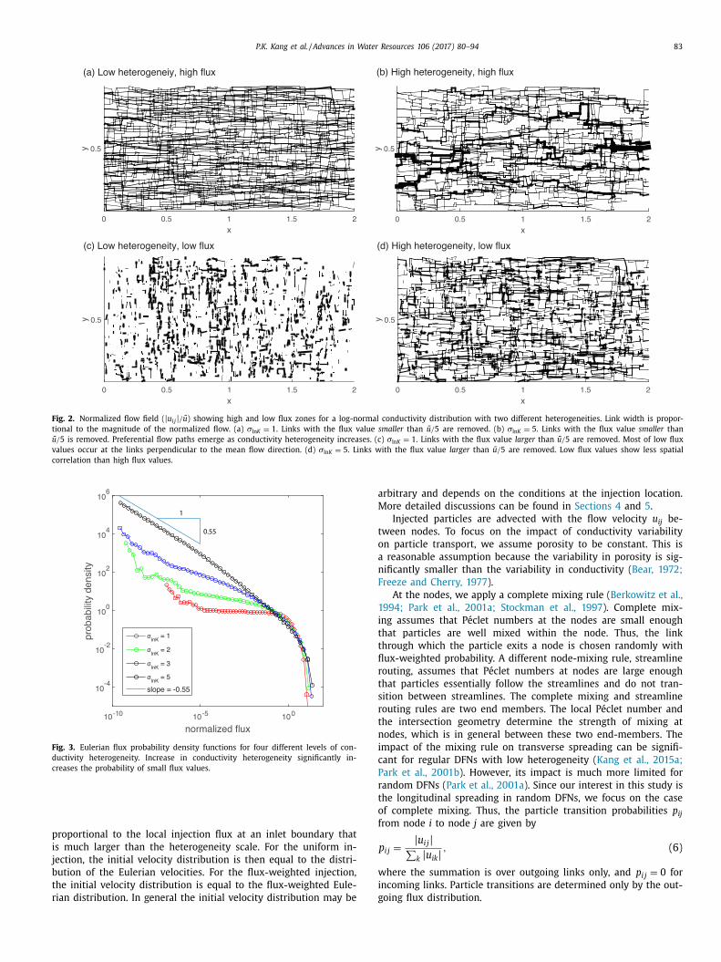
Fig. 2. Normalized flow field ( | u i j | / u ) showing high and low flux zones for a log-normal conductivity distribution with two different heterogeneities. Link width is propor-

tional to the magnitude of the normalized flow. (a) σln K = 1 . Links with the flux value smaller than u / 5 are removed. (b) σln K = 5 . Links with the flux value smaller than

u / 5 is removed. Preferential flow paths emerge as conductivity heterogeneity increases. (c) σln K = 1 . Links with the flux value larger than u / 5 are removed. Most of low flux

values occur at the links perpendicular to the mean flow direction. (d) σln K = 5 . Links with the flux value larger than u / 5 are removed. Low flux values show less spatial

correlation than high flux values.

Fig. 3. Eulerian flux probability density functions for four different levels of con-

ductivity heterogeneity. Increase in conductivity heterogeneity significantly in-

creases the probability of small flux values.

p

i

j

b

t

r

a

M

t

o

a

n

F

1

i

t

t

fl

r

t

s

r

t

n

i

c

P

r

t

o

f

w

i

g

roportional to the local injection flux at an inlet boundary that

s much larger than the heterogeneity scale. For the uniform in-

ection, the initial velocity distribution is then equal to the distri-

ution of the Eulerian velocities. For the flux-weighted injection,

he initial velocity distribution is equal to the flux-weighted Eule-

ian distribution. In general the initial velocity distribution may be

rbitrary and depends on the conditions at the injection location.

ore detailed discussions can be found in Sections 4 and 5 .

Injected particles are advected with the flow velocity u ij be-

ween nodes. To focus on the impact of conductivity variability

n particle transport, we assume porosity to be constant. This is

reasonable assumption because the variability in porosity is sig-

ificantly smaller than the variability in conductivity ( Bear, 1972;

reeze and Cherry, 1977 ).

At the nodes, we apply a complete mixing rule ( Berkowitz et al.,

994; Park et al., 2001a; Stockman et al., 1997 ). Complete mix-

ng assumes that Péclet numbers at the nodes are small enough

hat particles are well mixed within the node. Thus, the link

hrough which the particle exits a node is chosen randomly with

ux-weighted probability. A different node-mixing rule, streamline

outing, assumes that Péclet numbers at nodes are large enough

hat particles essentially follow the streamlines and do not tran-

ition between streamlines. The complete mixing and streamline

outing rules are two end members. The local Péclet number and

he intersection geometry determine the strength of mixing at

odes, which is in general between these two end-members. The

mpact of the mixing rule on transverse spreading can be signifi-

ant for regular DFNs with low heterogeneity ( Kang et al., 2015a;

ark et al., 2001b ). However, its impact is much more limited for

andom DFNs ( Park et al., 2001a ). Since our interest in this study is

he longitudinal spreading in random DFNs, we focus on the case

f complete mixing. Thus, the particle transition probabilities p ij rom node i to node j are given by

p i j =

| u i j | ∑

k | u ik | , (6)

here the summation is over outgoing links only, and p i j = 0 for

ncoming links. Particle transitions are determined only by the out-

oing flux distribution.

84 P.K. Kang et al. / Advances in Water Resources 106 (2017) 80–94

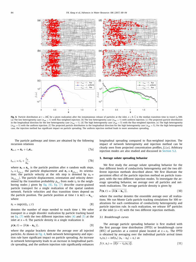
Fig. 4. Particle distribution at t = 20 t l for a given realization after the instantaneous release of particles at the inlet, x = 0 . t l is the median transition time to travel L x /100.

(a) The low heterogeneity case ( σln K = 1 ) with flux-weighted injection. (b) The low heterogeneity case ( σln K = 1 ) with uniform injection. (c) The projected particle distribution

in the longitudinal direction for the low heterogeneity case ( σln K = 1 ). (d) The high heterogeneity case ( σln K = 5 ) with the flux-weighted injection. (e) The high heterogeneity

( σln K = 5 ) with the uniform injection. (f) The projected particle distribution in the longitudinal direction for the high heterogeneity case ( σln K = 5 ). For the high heterogeneity

case, the injection method has significant impact on particle spreading. The uniform injection method leads to more anomalous spreading.

t

l

i

c

i

3

f

f

p

p

e

w

P

w

t

a

p

a

3

t

(

i

τ

The particle pathways and times are obtained by the following

recursion relations

x n +1 = x n + � n e n , (7a)

n +1 = t n +

� n

u n , (7b)

where x n ≡ x i n is the particle position after n random walk steps,

� n ≡ l i n i n +1 the particle displacement and e n ≡ e i n i n +1

its orienta-

tion; the particle velocity at the n th step is denoted by u n ≡| u i n i n +1

| . The particle displacement, orientation and velocity deter-

mined by the transition probability p i n j from node i n to the neigh-

boring nodes j given by Eq. (6) . Eq. (7) describe coarse-grained

particle transport for a single realization of the spatial random

network. Particle velocities and thus transition times depend on

the particle position. The particle position at time t is x (t) = x i n t ,

where

n t = sup (n | t n ≤ t) (8)

denotes the number of steps needed to reach time t . We solve

transport in a single disorder realization by particle tracking based

on Eq. (7) with the two different injection rules (4) and (5) at the

inlet at x = 0 . The particle density in a single realization is

p(x , t) = 〈 δ(x − x n t ) 〉 , (9)

where the angular brackets denote the average over all injected

particles. As shown in Fig. 4 , both network heterogeneity and injec-

tion rule have significant impact on particle spreading. An increase

in network heterogeneity leads to an increase in longitudinal parti-

cle spreading, and the uniform injection rule significantly enhances

ongitudinal spreading compared to flux-weighted injection. The

mpact of network heterogeneity and injection method can be

learly seen from projected concentration profiles, f τ ( ω). Arbitrary

njection modes are also studied and discussed in Section 5.2 .

. Average solute spreading behavior

We first study the average solute spreading behavior for the

our different levels of conductivity heterogeneity and the two dif-

erent injection methods described above. We first illustrate the

ersistent effect of the particle injection method on particle trans-

ort, with the two different injection modes. To investigate the av-

rage spreading behavior, we average over all particles and net-

ork realizations. The average particle density is given by

(x , t) = 〈 δ(x − x n t ) 〉 , (10)

here the overbar denotes the ensemble average over all realiza-

ions. We run Monte Carlo particle tracking simulations for 100 re-

lizations for each combination of conductivity heterogeneity and

article injection rule. In each realization, we release 10 4 particles

t the inlet ( x = 0 ) with the two different injection methods.

.1. Breakthrough curves

The average particle spreading behavior is first studied with

he first passage time distribution (FPTD) or breakthrough curve

BTC) of particles at a control plane located at x = x c . The FPTD

s obtained by averaging over the individual particle arrival times

a (x c ) = inf (t n | | x n − x 0 | > x c ) as

f (τ, x c ) = 〈 δ[ τ − τa (x c )] 〉 . (11)

P.K. Kang et al. / Advances in Water Resources 106 (2017) 80–94 85

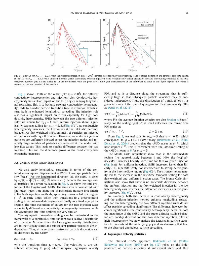
Fig. 5. (a) FPTDs for σln K = 1 , 2 , 3 , 5 with flux-weighted injection at x c = 200 l . Increase in conductivity heterogeneity leads to larger dispersion and stronger late-time tailing.

(b) FPTDs for σln K = 1 , 2 , 3 , 5 with uniform injection (black solid lines). Uniform injection leads to significantly larger dispersion and late-time tailing compared to the flux-

weighted injection (red dashed lines). FPTDs are normalized with the peak arrival time. (For interpretation of the references to color in this figure legend, the reader is

referred to the web version of this article.)

c

e

n

i

t

a

d

r

i

h

b

a

p

a

l

i

e

3

t

s

b

a

l

t

l

(

s

r

a

t

f

o

a

d

b

x

w

t

P

c

s

g

a

ψ

w

i

P

ψ

c

D

h

t

r

n

(

e

i

i

fl

u

t

h

i

a

i

a

c

t

i

h

t

t

4

B

p

Fig. 5 shows FPTDs at the outlet, f (τ, x c = 200 l ) , for different

onductivity heterogeneities and injection rules. Conductivity het-

rogeneity has a clear impact on the FPTD by enhancing longitudi-

al spreading. This is so because stronger conductivity heterogene-

ty leads to broader particle transition time distribution, which in

urn leads to enhanced longitudinal spreading. The injection rule

lso has a significant impact on FPTDs especially for high con-

uctivity heterogeneity. FPTDs between the two different injection

ules are similar for σln K = 1 , but uniform injection shows signif-

cantly stronger tailing for σln K = 2 , 3 , 5 ( Fig. 5 (b)). As conductivity

eterogeneity increases, the flux values at the inlet also becomes

roader. For flux-weighted injection, most of particles are injected

t the nodes with high flux values. However, for uniform injection,

articles are uniformly injected across the injection nodes and rel-

tively large number of particles are released at the nodes with

ow flux values. This leads to notable difference between the two

njection rules and the difference grows as the conductivity het-

rogeneity increases.

.2. Centered mean square displacement

We also study longitudinal spreading in terms of the cen-

ered mean square displacement (cMSD) of average particle den-

ity, P (x , t) . For the longitudinal direction ( x ), the cMSD is given

y σ 2 x (t) = 〈 [ x (t) − 〈 x (t) 〉 ] 2 〉 where 〈 · 〉 denotes the average over

ll particles for a given realization. In Fig. 6 , we show the time evo-

ution of the longitudinal cMSDs. The time axis is normalized with

he mean travel time along the characteristic fracture link length,

. For both injection methods, spreading shows a ballistic regime

∼ t 2 ) at early times, which then transitions to a preasymptotic

caling in an intermediate regime and finally to a final asymptotic

egime. The time evolutions of cMSDs for the two injection cases

re notably different as conductivity heterogeneity increases, while

he asymptotic late-time scalings are very similar.

The asymptotic power-law scaling can be understood in the

ramework of a continuous time random walk (CTRW) description

f dispersion. At large times the Lagrangian velocity distributions

re in their steady states and subsequent particle velocities are in-

ependent. Thus, at large times horizontal particle dispersion can

e described by the CTRW

n +1 = x n + � 0 , t n +1 = t n + τn , (12)

ith the transition time τn = � 0 / v n . The velocities v n are dis-

ributed according to p s ( v ) which is space Lagrangian velocity

DF, and � 0 is a distance along the streamline that is suffi-

iently large so that subsequent particle velocities may be con-

idered independent. Thus, the distribution of transit times τ n is

iven in terms of the space Lagrangian and Eulerian velocity PDFs

s Dentz et al. (2016)

(τ ) =

� 0

τ 2 p s (� 0 /τ ) =

� 0

τ 3 v p e (� 0 /τ ) , (13)

here v is the average Eulerian velocity, see also Section 4 . Specif-

cally, for the scaling p e ( v ) ∝ v α at small velocities, the transit time

DF scales as

(τ ) ∝ τ−1 −β, β = 2 + α. (14)

From Fig. 3 , we estimate for σln K = 5 that α ≈ −0 . 55 , which

orresponds to β = 1 . 45 . CTRW theory ( Berkowitz et al., 2006;

entz et al., 2004 ) predicts that the cMSD scales as t 3 −β, which

ere implies t 1.55 . This is consistent with the late-time scaling of

he cMSD shown in 6 for σln K = 5 .

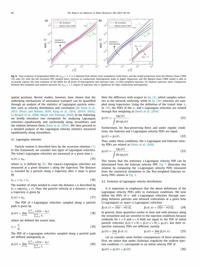
The Monte Carlo simulations show that, in the intermediate

egime ( t/ t l approximately between 1 and 100), the longitudi-

al cMSD increases linearly with time for flux-weighted injection

Fig. 6 (a)). For uniform injection, cMSD increases faster than lin-

arly (i.e., superdiffusively) for intermediate to strong heterogene-

ty in the intermediate regime ( Fig. 6 (b)). The stronger heterogene-

ty led to the increase in the late-time temporal scaling for both

ux-weighted and uniform injection cases. The Monte Carlo sim-

lations also show that there is no noticeable difference between

he uniform injection and the flux-weighted injection for the low

eterogeneity case whereas the difference increases as heterogene-

ty increases ( Fig. 6 (b), inset).

In summary, both the increase in conductivity heterogeneity

nd the uniform injection method enhance longitudinal spread-

ng. For low heterogeneity, the two different injection rules do not

ffect particle spreading significantly. The difference, however, be-

omes significant as the conductivity heterogeneity increases. Both

he magnitude of the cMSD and the super-diffusive scaling behav-

or are notably different for the two different injection rules at

igh heterogeneity. We now analyze the Lagrangian particle statis-

ics to understand the underlying physical mechanisms that lead

o the observed anomalous particle spreading.

. Lagrangian velocity statistics

The classical CTRW approach Berkowitz et al. (2006) ;

erkowitz and Scher (1997) —see Eq. (12) —relies on the inde-

endence of particle velocities at subsequent steps and thus

86 P.K. Kang et al. / Advances in Water Resources 106 (2017) 80–94

Fig. 6. Time evolution of longitudinal MSDs for σln K = 1 , 2 , 3 , 5 obtained from Monte Carlo simulations (solid lines), and the model predictions from the Markov-Chain CTRW

(32) and (35) with the full transition PDF (dashed lines). Increase in conductivity heterogeneity leads to higher dispersion, and the Markov-chain CTRW model is able to

accurately capture the time evolution of the MSDs for all levels of heterogeneity and injection rules. (a) Flux-weighted injection. (b) Uniform injection. Inset: Comparison

between flux-weighted and uniform injection for σln K = 1 , 5 . Impact of injection rule is significant for high conductivity heterogeneity.

N

t

p

i

t

F

t

T

i

T

d

r

f

l

4

L

d

p

(

I

t

e

p

s

F

t

spatial positions. Recent studies, however, have shown that the

underlying mechanisms of anomalous transport can be quantified

through an analysis of the statistics of Lagrangian particle veloc-

ities such as velocity distribution and correlation ( de Anna et al.,

2013; Dentz and Bolster, 2010; Kang et al., 2014; 2011b; 2015a;

Le Borgne et al., 2008; Meyer and Tchelepi, 2010 ). In the following,

we briefly introduce two viewpoints for analyzing Lagrangian

velocities—equidistantly and isochronally along streamlines—and

the relation between them Dentz et al. (2016) . We then proceed to

a detailed analysis of the Lagrangian velocity statistics measured

equidistantly along streamlines.

4.1. Lagrangian velocities

Particle motion is described here by the recursion relations (7) .

In this framework, we consider two types of Lagrangian velocities.

The t(ime)–Lagrangian velocities are measured at a given time t ,

v t (t) = u n t , (15)

where n t is defined by (8) . The s(pace)–Lagrangian velocities are

measured at a given distance s along the trajectory. The distance

s n traveled by a particle along a trajectory after n steps is given

by

s n +1 = s n + � n . (16)

The number of steps needed to cover the distance s is described by

n s = sup (n | s n ≤ s ) . Thus, the particle velocity at a distance s along

a trajectory is given by

v s (s ) = u n s . (17)

The PDF of t–Lagrangian velocities sampled along a particle

path is given by

p t (v ) = lim

n →∞

∑ n i =1 τi δ(v − u i ) ∑ n

i =1 τi

, (18)

where we defined the transit time,

τi =

� i

u i

(19)

The PDF of s–Lagrangian velocities sampled along a particle path

are defined analogously as

p s (v ) = lim

n →∞

∑ n i =1 � i δ(v − u i ) ∑ n

� i . (20)

i =1

ote the difference with respect to Eq. (2) , which samples veloci-

ies in the network uniformly, while in Eq. (20) velocities are sam-

led along trajectories. Using the definition of the transit time τ i

n (19) , the PDFs of the s– and t–Lagrangian velocities are related

hrough flux weighting as Dentz et al. (2016)

p s (v ) =

v p t (v ) ∫ dv v p t (v )

. (21)

urthermore, for flux-preserving flows and under ergodic condi-

ions, the Eulerian and t-Lagrangian velocity PDFs are equal,

p e (v ) = p t (v ) . (22)

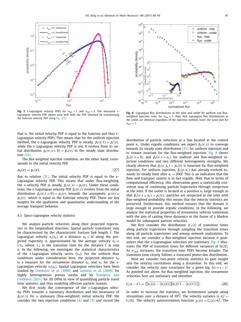
hus, under these conditions, the s–Lagrangian and Eulerian veloc-

ty PDFs are related as Dentz et al. (2016)

p s (v ) =

v p e (v ) ∫ dv v p e (v )

. (23)

his means that the stationary s-Lagrangian velocity PDF can be

etermined from the Eulerian velocity PDF. Fig. 7 illustrates this

elation by comparing the s-Lagrangian velocity PDFs measured

rom the numerical simulation to the flux-weighted Eulerian ve-

ocity PDFs shown in Fig. 3 .

.2. Evolution of Lagrangian velocity distributions

It is important to emphasize that the above definitions of the

agrangian velocity PDFs refer to stationary conditions. We now

efine the PDFs of t– and s–Lagrangian velocities through sam-

ling between particles and network realizations at a given time

t-Lagrangian) or space (s-Lagrangian) velocities

ˆ p t (v , t) = 〈 δ[ v − v (t)] 〉 , ˆ p s (v , s ) = 〈 δ[ v − v (s )] 〉 . (24)

n general, these quantities evolve in time and with distance along

he streamline and are sensitive to the injection conditions because

vidently for t = 0 and s = 0 both are equal to the PDF of initial

article velocities ˆ p t (v , t = 0) = ˆ p s (v , s = 0) = p 0 (v ) , but their re-

pective stationary PDFs are different, namely

p t (v ) = lim

t→∞

ˆ p t (v , t) , p s (v ) = lim

s →∞

ˆ p s (v , s ) . (25)

Let us consider some further consequences of these properties.

irst, we notice that under (Eulerian) ergodicity the uniform injec-

ion condition (4) corresponds to an initial velocity PDF of

p 0 (v ) = p e (v ) = p t (v ) , (26)

P.K. Kang et al. / Advances in Water Resources 106 (2017) 80–94 87

Fig. 7. s-Lagrangian velocity PDFs for σln K = 1 and σln K = 5 . The measured s-

Lagrangian velocity PDF agrees very well with the PDF obtained by transforming

the Eulerian velocity PDF using Eq. (23) .

t

L

m

w

t

t

s

d

L

t

t

d

i

a

4

r

b

L

j

l

n

o

c

i

L

s

h

C

t

i

c

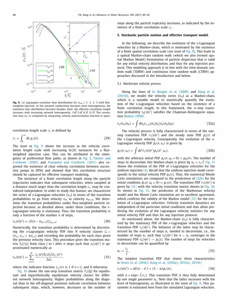
Fig. 8. Lagrangian flux distributions at the inlet and outlet for uniform and flux-

weighted injection rules, for σln K = 5 . Note that Lagrangian flux distributions at

the outlet are identical regardless of the injection method. Inset: the same plot for

σln K = 1 .

d

p

t

t

j

c

i

w

fl

c

s

a

t

fl

p

l

a

w

m

a

a

t

a

t

A

t

i

c

A

v

C

I

s

C

hat is, the initial velocity PDF is equal to the Eulerian and thus t–

agrangian velocity PDFs. This means that for the uniform injection

ethod, the t–Lagrangian velocity PDF is steady, ˆ p t (v , t) = p t (v ) ,hile the s–Lagrangian velocity PDF is not. It evolves from its ini-

ial distribution p s (v , s = 0) = p e (v ) to the steady state distribu-

ion (23) .

The flux-weighted injection condition, on the other hand, corre-

ponds to the initial velocity PDF

p 0 (v ) = p s (v ) , (27)

ue to relation (21) . The initial velocity PDF is equal to the s–

agrangian velocity PDF. This means that under flux-weighting,

he s–velocity PDF is steady, ˆ p s (v , s ) = p s (v ) . Under these condi-

ions, the t–Lagrangian velocity PDF ˆ p t (v , t) evolves from the initial

istribution ˆ p t (v , t = 0) = p s (v ) towards the asymptotic p t (v ) =p e (v ) , which is equal to the Eulerian velocity PDF. These are key

nsights for the qualitative and quantitative understanding of the

verage transport behavior.

.3. Space-Lagrangian velocity statistics

We analyze particle velocities along their projected trajecto-

ies in the longitudinal direction. Spatial particle transitions may

e characterized by the characteristic fracture link length, l . The

agrangian velocity v s ( s n ) at a distance x n = n l along the pro-

ected trajectory is approximated by the average velocity v n ≡ /τn where τ n is the transition time for the distance l at step

. In the following, we investigate the statistical characteristics

f the s-Lagrangian velocity series { v n }. For the uniform flow

onditions under consideration here, the projected distance x n s a measure for the streamwise distance s n , and v n for the s-

agrangian velocity v s ( s n ). Spatial Lagrangian velocities have been

tudied by Cvetkovic et al. (1996) and Gotovac et al. (2009) for

ighly heterogeneous porous media and by Frampton and

vetkovic (2011) for 3D DFNs in view of quantifying particle travel

ime statistics and thus modeling effective particle motion.

We first study the convergence of the s–Lagrangian veloc-

ty PDFs towards a stationary distribution and the invariance of

ˆ p s (v , s ) for a stationary (flux-weighted) initial velocity PDF. We

onsider the two injection conditions (4) and (5) and record the

istribution of particle velocities at a line located at the control

oint x c . Under ergodic conditions, we expect ˆ p s (v , s ) to converge

owards its steady state distribution (23) for uniform injection and

o remain invariant for the flux-weighted injection. Fig. 8 shows

ˆ p s (v , s = 0) and ˆ p s (v , s = x c ) for uniform and flux-weighted in-

ection conditions and two different heterogeneity strengths. We

learly observe that ˆ p s (v , x c ) = p s (v ) is invariant for flux-weighted

njection. For uniform injection, ˆ p s (v , x c ) has already evolved to-

ards its steady limit after x c = 200 l . This is an indication that the

ow and transport system is in fact ergodic. Note that in terms of

omputational efficiency, this observation gives a statistically con-

istent way of continuing particle trajectories through reinjection

t the inlet. If the outlet is located at a position x c large enough so

hat ˆ p s (v , s = x c ) = p s (v ) , particles are reinjected at the inlet with

ux-weighted probability, this means that the velocity statistics are

reserved. Furthermore, this method ensures that the domain is

arge enough to provide ergodic conditions. In the following, we

nalyze the statistical properties of streamwise velocity transitions

ith the aim of casting these dynamics in the frame of a Markov

odel for subsequent particle velocities.

We first consider the distribution ψ τ ( t ) of transition times

long particle trajectories through sampling the transition times

long all particle trajectories and among network realizations. To

his end, we consider a flux-weighted injection because it guar-

ntees that the s-Lagranagian velocities are stationary. Fig. 9 illus-

rates the PDF of transition times for different variances of ln ( K ).

s σ ln K increases, the transition time PDFs become broader. The

ransition time closely follows a truncated power-law distribution.

Next we consider two-point velocity statistics to gain insight

nto the velocity correlations along a streamline. To this end, we

onsider the velocity auto covariance for a given lag �s = s − s ′ .s pointed out above, for flux-weighted injection, the streamwise

elocities here are stationary and therefore

s (s − s ′ ) = 〈 [ v s (s ) − 〈 v s (s ) 〉 ][ v s (s ′ ) − 〈 v s (s ′ ) 〉 ] 〉 . (28)

n order to increase the statistics, we furthermore sample along

treamlines over a distance of 10 2 l . The velocity variance is σ 2 v =

s (0) . The velocity autocorrelation function χs (s ) = C s (s ) /σ 2 v . The

88 P.K. Kang et al. / Advances in Water Resources 106 (2017) 80–94

Fig. 9. (a) Lagrangian transition time distributions for σln K = 1 , 2 , 3 , 5 with flux-

weighted injection. As the network conductivity becomes more heterogeneous, the

transition time distribution becomes broader. Inset: the effective correlation length

increases with increasing network heterogeneity: 3 . 8 l , 5 . 6 l , 8 . 2 l , 11 . 5 l . The correla-

tion step ( n c ) is computed by integrating velocity autocorrelation function in space.

s

i

5

v

o

a

t

f

t

d

p

5

(

w

t

fi

t

t

r

s

t

L

w

s

s

u

s

C

i

g

A

m

w

l

i

d

i

i

t

t

n

s

t

n

T

i

r

w

b

l

r

correlation length scale � c is defined by

� c =

∫ ∞

0

ds χs (s ) . (29)

The inset in Fig. 9 shows the increase in the velocity corre-

lation length scale with increasing ln ( K ) variances for a flux-

weighted injection case. This can be attributed to the emer-

gence of preferential flow paths, as shown in Fig. 2 . Painter and

Cvetkovic (2005) and Frampton and Cvetkovic (2011) also re-

ported the existence of clear velocity correlation between succes-

sive jumps in DFNs and showed that this correlation structure

should be captured for effective transport modeling.

The existence of a finite correlation length along the particle

trajectories indicates that subsequent velocities, when sampled at

a distance much larger than the correlation length � c , may be con-

sidered independent. In order to study this feature, we characterize

the series of s-Lagrangian velocities { v n } in terms of the transition

probabilities to go from velocity v m

to velocity v m + n . We deter-

mine the transition probabilities under flux-weighted particle in-

jection because, as detailed above, under these conditions, the s-

Lagrangian velocity is stationary. Thus, the transition probability is

only a function of the number n of steps,

r n (v | v ′ ) = 〈 δ(v − v m + n ) 〉 | v m = v ′ (30)

Numerically, the transition probability is determined by discretiz-

ing the s-Lagrangian velocity PDF into N velocity classes C i =(v s,i , v s,i + �v s,i ) and recording the probability for each class given

the previous velocity class. This procedure gives the transition ma-

trix T n ( i | j ) from class j to i after n steps such that r n ( v | v ′ ) is ap-

proximated numerically as

r n (v | v ′ ) =

N ∑

i, j=1

I C i (v ) T n (i | j) I C j (v ′ ) �v i

, (31)

where the indicator function I C i (v ) is 1 if v ∈ C i and 0 otherwise.

Fig. 10 shows the one-step transition matrix T 1 ( i | j ) for equidis-

tant and logarithmically equidistant velocity classes for differ-

ent network heterogeneity. Higher probabilities along the diago-

nal than in the off-diagonal positions indicate correlation between

subsequent steps, which, however, decreases as the number of

teps along the particle trajectory increases, as indicated by the ex-

stence of a finite correlation scale � c .

. Stochastic particle motion and effective transport model

In the following, we describe the evolution of the s-Lagrangian

elocities by a Markov-chain, which is motivated by the existence

f a finite spatial correlation scale (see inset of Fig. 9 ). This leads to

spatial Markov-chain random walk (which we also termed spa-

ial Markov Model) formulation of particle dispersion that is valid

or any initial velocity distribution, and thus for any injection pro-

ocol. This modeling approach is in line with the time-domain ran-

om walk (TDRW) and continuous time random walk (CTRW) ap-

roaches discussed in the Introduction and below.

.1. Markovian velocity process

Along the lines of Le Borgne et al. (2008) and Kang et al.

2011b ), we model the velocity series { v n } as a Markov-chain,

hich is a suitable model to statistically quantify the evolu-

ion of the s-Lagrangian velocities based on the existence of a

nite correlation length. In this framework, the n –step transi-

ion probability r n ( v | v ′ ) satisfies the Chapman–Kolmogorov equa-

ion Risken (1996)

n (v n | v 0 ) =

∫ dv k r n −k (v n | v k ) r k (v k | v 0 ) . (32a)

The velocity process is fully characterized in terms of the one-

tep transition PDF r 1 ( v | v ′ ) and the steady state PDF p s ( v ) of

he s-Lagrangian velocity. Consequently, the evolution of the s-

agrangian velocity PDF ˆ p s (v , s n ) is given by

p s (v , s n ) =

∫ dv ′ r 1 (v | v ′ ) p s (v ′ , s n ) , (32b)

ith the arbitrary initial PDF p s (v , s 0 = 0) = p 0 (v ) . The number of

teps to decorrelate this Markov-chain is given by n c = � c / l . Fig. 11

hows the evolution of the PDF of s-Lagrangian velocities for the

niform injection (4) . Recall that the uniform injection mode corre-

ponds to the initial velocity PDF p e ( v ). Thus, the numerical Monte

arlo simulations are compared to the predictions of (32b) for the

nitial condition ˆ p s (v , s 0 = 0) = p e (v ) . The transition PDF r 1 ( v | v ′ ) is

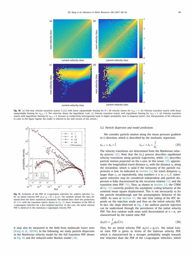
iven by (31) with the velocity transition matrix shown in Fig. 10 .

s shown in Fig. 11 , the prediction of the Markovian velocity

odel and the Monte Carlo simulation are in excellent agreement,

hich confirms the validity of the Markov model (32) for the evo-

ution of s-Lagrangian velocities. Velocity transition dynamics are

ndependent of the particular initial conditions and thus allow pre-

icting the evolution of the Lagrangian velocity statistics for any

nitial velocity PDF and thus for any injection protocol.

As mentioned above, the Markov-chain { v n } is fully character-

zed by the stationary PDF of the s-Lagrangian velocities and the

ransition PDF r 1 ( v | v ′ ). The behavior of the latter may be charac-

erized by the number of steps n c needed to decorrelate, i.e., the

umber of steps n c such that r n ( v | v ′ ) for n > n c converges to the

tationary PDF r n ( v | v ′ ) → p s ( s ). The number of steps for velocities

o decorrelate can be quantified by

c =

� c

l , (33)

he simplest transition PDF that shares these characteristics

s Dentz et al. (2016) ; Kang et al. (2016a) ; 2015a) ; 2015b)

1 (v | v ′ ) = aδ(v − v ′ ) + (1 − a ) p s (v ) , (34)

ith a = exp (−l /� c ) . This transition PDF is thus fully determined

y one single parameter n c . Note that the latter increases with the

evel of heterogeneity, as illustrated in the inset of Fig. 9 . This pa-

ameter is estimated here from the simulated Lagrangian velocities.

P.K. Kang et al. / Advances in Water Resources 106 (2017) 80–94 89

Fig. 10. (a) One-step velocity transition matrix T 1 ( i | j ) with linear equiprobable binning for N = 50 velocity classes for σln K = 1 . (b) Velocity transition matrix with linear

equiprobable binning for σln K = 5 . The color-bar shows the logarithmic scale. (c) Velocity transition matrix with logarithmic binning for σln K = 1 . (d) Velocity transition

matrix with logarithmic binning for σln K = 5 . Increase in conductivity heterogeneity leads to higher probability close to diagonal entries. (For interpretation of the references

to color in this figure legend, the reader is referred to the web version of this article.)

Fig. 11. Evolution of the PDF of s-Lagrangian velocities for uniform injection , i.e.,

for an initial velocity PDF ˆ p s (v , s 0 = 0) = p e (v ) . The symbols denote the data ob-

tained from the direct numerical simulation, the dashed lines show the predictions

of (32b) with the transition matrix shown in Fig. 10 . Inset: Evolution of the PDF of

s-Lagrangian velocities for a flux-weighted injection . In this case, the initial velocity

PDF is identical to the stationary s-Lagrangian velocity PDF.

I

(

i

i

5

i

x

T

i

v

p

m

t

j

l

q

p

t

o

c

t

c

p

I

c

P

c

ψ

T

s

w

l

t may also be measured in the field from multiscale tracer tests

Kang et al., 2015b ). In the following, we study particle dispersion

n the Markovian velocity model for the full transition PDF shown

n Fig. 10 and the reduced-order Markov model (34) .

.2. Particle dispersion and model predictions

We consider particle motion along the mean pressure gradient

n x –direction, which is described by the stochastic regression

n +1 = x n + l , t n +1 = t n +

l

v n . (35)

he velocity transitions are determined from the Markovian veloc-

ty process (32) . Note that the { v n } process describes equidistant

elocity transitions along particle trajectories, while (35) describes

article motion projected on the x -axis. In this sense, (35) approxi-

ates the longitudinal travel distance x n with the distance s n along

he streamline, which is valid if the tortuosity of the particle tra-

ectories is low. As indicated in Section 3.2 , for travel distances � 0 arger than � c , or equivalently, step numbers n � n c ≡ � c / l , subse-

uent velocities may be considered independent and particle dis-

ersion is fully characterized by the recursion relation (12) and the

ransition time PDF (13) . Thus, as shown in Section 3.2 , the CTRW

f Eq. (12) correctly predicts the asymptotic scaling behavior of the

entered mean square displacement. This is not necessarily so for

he particle breakthrough and the preasymptotic behavior of the

MSD. As seen in Section 3.1 , the late time tailing of the BTC de-

ends on the injection mode and thus on the initial velocity PDF.

n fact, the slope observed in Fig. 5 for uniform particle injection

an be understood through the persistence of the initial velocity

DF. The first random walk steps until decorrelation at n = n c are

haracterized by the transit time PDF

0 (t ) =

l

t 2 p 0 ( l /t ) . (36)

hus, for an initial velocity PDF p 0 (v ) = p e (v ) , the initial tran-

it time PDF is given in terms of the Eulerian velocity PDF,

hich is characterized by a stronger probability weight towards

ow velocities than the PDF of the s-Lagrangian velocities, which

90 P.K. Kang et al. / Advances in Water Resources 106 (2017) 80–94

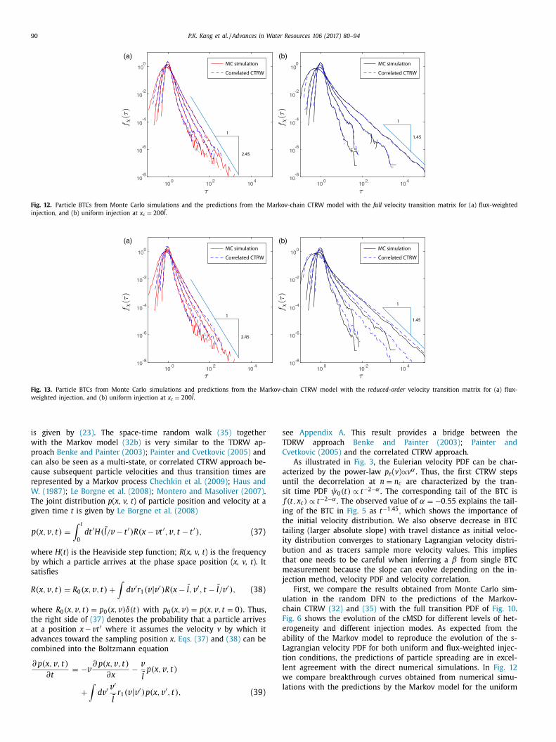
Fig. 12. Particle BTCs from Monte Carlo simulations and the predictions from the Markov-chain CTRW model with the full velocity transition matrix for (a) flux-weighted

injection, and (b) uniform injection at x c = 200 l .

Fig. 13. Particle BTCs from Monte Carlo simulations and predictions from the Markov-chain CTRW model with the reduced-order velocity transition matrix for (a) flux-

weighted injection, and (b) uniform injection at x c = 200 l .

s

T

C

a

u

s

i

t

t

i

b

t

m

j

u

c

F

e

a

L

t

l

w

l

is given by (23) . The space-time random walk (35) together

with the Markov model (32b) is very similar to the TDRW ap-

proach Benke and Painter (2003) ; Painter and Cvetkovic (2005) and

can also be seen as a multi-state, or correlated CTRW approach be-

cause subsequent particle velocities and thus transition times are

represented by a Markov process Chechkin et al. (2009) ; Haus and

W. (1987) ; Le Borgne et al. (2008) ; Montero and Masoliver (2007) .

The joint distribution p ( x, v, t ) of particle position and velocity at a

given time t is given by Le Borgne et al. (2008)

p(x, v , t) =

∫ t

0

dt ′ H( l / v − t ′ ) R (x − v t ′ , v , t − t ′ ) , (37)

where H ( t ) is the Heaviside step function; R ( x, v, t ) is the frequency

by which a particle arrives at the phase space position ( x, v, t ). It

satisfies

R (x, v , t) = R 0 (x, v , t) +

∫ dv ′ r 1 (v | v ′ ) R (x − l , v ′ , t − l / v ′ ) , (38)

where R 0 (x, v , t) = p 0 (x, v ) δ(t) with p 0 (x, v ) = p(x, v , t = 0) . Thus,

the right side of (37) denotes the probability that a particle arrives

at a position x − v t ′ where it assumes the velocity v by which it

advances toward the sampling position x . Eqs. (37) and (38) can be

combined into the Boltzmann equation

∂ p(x, v , t) ∂t

= −v ∂ p(x, v , t)

∂x − v

l p(x, v , t)

+

∫ dv ′ v

′ ¯

r 1 (v | v ′ ) p(x, v ′ , t) , (39)

l

ee Appendix A . This result provides a bridge between the

DRW approach Benke and Painter (2003) ; Painter and

vetkovic (2005) and the correlated CTRW approach.

As illustrated in Fig. 3 , the Eulerian velocity PDF can be char-

cterized by the power-law p e ( v ) ∝ v α . Thus, the first CTRW steps

ntil the decorrelation at n = n c are characterized by the tran-

it time PDF ψ 0 (t) ∝ t −2 −α . The corresponding tail of the BTC is

f (t, x c ) ∝ t −2 −α . The observed value of α = −0 . 55 explains the tail-

ng of the BTC in Fig. 5 as t −1 . 45 , which shows the importance of

he initial velocity distribution. We also observe decrease in BTC

ailing (larger absolute slope) with travel distance as initial veloc-

ty distribution converges to stationary Lagrangian velocity distri-

ution and as tracers sample more velocity values. This implies

hat one needs to be careful when inferring a β from single BTC

easurement because the slope can evolve depending on the in-

ection method, velocity PDF and velocity correlation.

First, we compare the results obtained from Monte Carlo sim-

lation in the random DFN to the predictions of the Markov-

hain CTRW (32) and (35) with the full transition PDF of Fig. 10 .

ig. 6 shows the evolution of the cMSD for different levels of het-

rogeneity and different injection modes. As expected from the

bility of the Markov model to reproduce the evolution of the s-

agrangian velocity PDF for both uniform and flux-weighted injec-

ion conditions, the predictions of particle spreading are in excel-

ent agreement with the direct numerical simulations. In Fig. 12

e compare breakthrough curves obtained from numerical simu-

ations with the predictions by the Markov model for the uniform

P.K. Kang et al. / Advances in Water Resources 106 (2017) 80–94 91

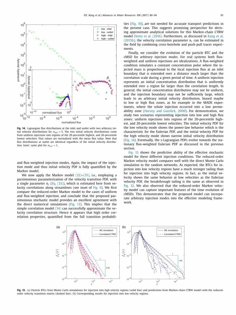
Fig. 14. Lagrangian flux distributions at the inlet and outlet with two arbitrary ini-

tial velocity distributions for σln K = 5 . The two initial velocity distributions come

from uniform injections into regions of the 20-percentile highest, and 20-percentile

lowest velocities. Flux values are normalized with the mean flux value. Note that

flux distributions at outlet are identical regardless of the initial velocity distribu-

tion. Inset: same plot for σln K = 1 .

a

t

M

p

a

l

c

a

s

t

s

l

r

t

t

i

m

(

t

m

c

w

c

j

b

c

r

e

g

a

l

t

i

a

s

z

e

t

c

t

(

t

s

m

M

s

j

f

l

v

F

i

c

r

w

F

o

nd flux-weighted injection modes. Again, the impact of the injec-

ion mode and thus initial velocity PDF is fully quantified by the

arkov model.

We now apply the Markov model (32) –(35) , i.e., employing a

arsimonious parameterization of the velocity transition PDF, with

single parameter n c ( Eq. (33) ), which is estimated here from ve-

ocity correlations along streamlines (see inset of Fig. 9 ). We first

ompare the reduced-order Markov model to the cases of uniform

nd flux-weighted injection, and conclude that the proposed par-

imonious stochastic model provides an excellent agreement with

he direct numerical simulations ( Fig. 13 ). This implies that the

imple correlation model (34) can successfully approximate the ve-

ocity correlation structure. Hence it appears that high order cor-

elation properties, quantified from the full transition probabili-

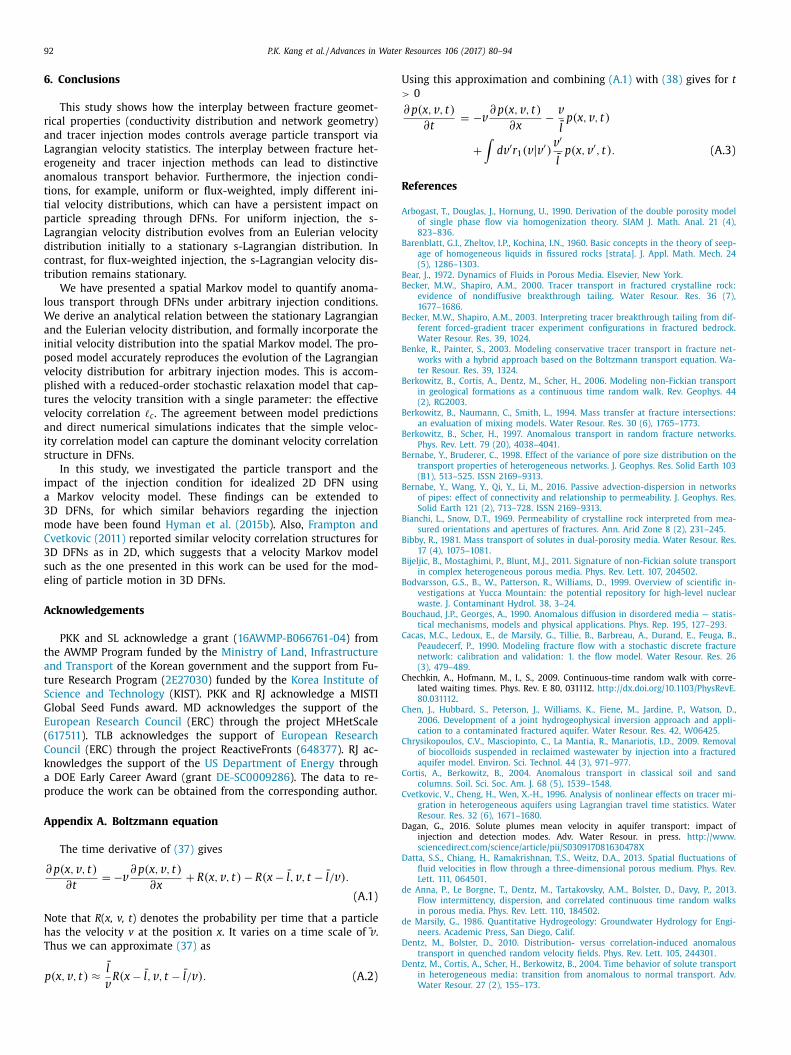
ig. 15. (a) Particle BTCs from Monte Carlo simulations for injection into high-velocity regi

rder velocity transition matrix (dashed line). (b) Corresponding results for injection into

ies ( Fig. 10 ), are not needed for accurate transport predictions in

he present case. This suggests promising perspective for deriv-

ng approximate analytical solutions for this Markov-chain CTRW

odel Dentz et al. (2016) . Furthermore, as discussed in Kang et al.

2015b ), the velocity correlation parameter n c can be estimated in

he field by combining cross-borehole and push-pull tracer experi-

ents.

Finally, we consider the evolution of the particle BTC and the

MSD for arbitrary injection modes . For real systems both flux-

eighted and uniform injections are idealizations. A flux-weighted

ondition simulates a constant concentration pulse where the in-

ected mass is proportional to the local injection flux at an inlet

oundary that is extended over a distance much larger than the

orrelation scale during a given period of time. A uniform injection

epresents an initial concentration distribution that is uniformly

xtended over a region far larger than the correlation length. In

eneral, the initial concentration distribution may not be uniform,

nd the injection boundary may not be sufficiently large, which

eads to an arbitrary initial velocity distribution, biased maybe

o low or high flux zones, as for example in the MADE exper-

ments, where the solute injection occurred into a low perme-

bility zone ( Harvey and Gorelick, 20 0 0 ). For demonstration, we

tudy two scenarios representing injection into low and high flux

ones: uniform injections into regions of the 20-percentile high-

st, and 20-percentile lowest velocities. The initial velocity PDF for

he low velocity mode shows the power-law behavior which is the

haracteristic for the Eulerian PDF, and the initial velocity PDF for

he high velocity mode shows narrow initial velocity distribution

Fig. 14 ). Eventually, the s-Lagrangian PDFs evolve towards the sta-

ionary flux-weighted Eulerian PDF as discussed in the previous

ection.

Fig. 15 shows the predictive ability of the effective stochastic

odel for these different injection conditions. The reduced-order

arkov velocity model compares well with the direct Monte Carlo

imulation in the random networks. As expected, the BTCs for in-

ection into low velocity regions have a much stronger tailing than

or injection into high velocity regions. In fact, as the initial ve-

ocity shows the same behavior at low velocities as the Eulerian

elocity PDF, the breakthrough tailing is the same as observed in

ig. 12 . We also observed that the reduced-order Markov veloc-

ty model can capture important features of the time evolution of

MSDs. This demonstrates that the proposed model can incorpo-

ate arbitrary injection modes into the effective modeling frame-

ork.

ons (solid line) and predictions from Markov-chain CTRW model with the reduced-

low-velocity regions.

92 P.K. Kang et al. / Advances in Water Resources 106 (2017) 80–94

U

>

R

A

B

B

B

B

B

B

B

B

B

B

B

B

C

C

C

C

C

D

6. Conclusions

This study shows how the interplay between fracture geomet-

rical properties (conductivity distribution and network geometry)

and tracer injection modes controls average particle transport via

Lagrangian velocity statistics. The interplay between fracture het-

erogeneity and tracer injection methods can lead to distinctive

anomalous transport behavior. Furthermore, the injection condi-

tions, for example, uniform or flux-weighted, imply different ini-

tial velocity distributions, which can have a persistent impact on

particle spreading through DFNs. For uniform injection, the s-

Lagrangian velocity distribution evolves from an Eulerian velocity

distribution initially to a stationary s-Lagrangian distribution. In

contrast, for flux-weighted injection, the s-Lagrangian velocity dis-

tribution remains stationary.

We have presented a spatial Markov model to quantify anoma-

lous transport through DFNs under arbitrary injection conditions.

We derive an analytical relation between the stationary Lagrangian

and the Eulerian velocity distribution, and formally incorporate the

initial velocity distribution into the spatial Markov model. The pro-

posed model accurately reproduces the evolution of the Lagrangian

velocity distribution for arbitrary injection modes. This is accom-

plished with a reduced-order stochastic relaxation model that cap-

tures the velocity transition with a single parameter: the effective

velocity correlation � c . The agreement between model predictions

and direct numerical simulations indicates that the simple veloc-

ity correlation model can capture the dominant velocity correlation

structure in DFNs.

In this study, we investigated the particle transport and the

impact of the injection condition for idealized 2D DFN using

a Markov velocity model. These findings can be extended to

3D DFNs, for which similar behaviors regarding the injection

mode have been found Hyman et al. (2015b ). Also, Frampton and

Cvetkovic (2011) reported similar velocity correlation structures for

3D DFNs as in 2D, which suggests that a velocity Markov model

such as the one presented in this work can be used for the mod-

eling of particle motion in 3D DFNs.

Acknowledgements

PKK and SL acknowledge a grant ( 16AWMP-B0 6 6761-04 ) from

the AWMP Program funded by the Ministry of Land, Infrastructure

and Transport of the Korean government and the support from Fu-

ture Research Program ( 2E27030 ) funded by the Korea Institute of

Science and Technology (KIST). PKK and RJ acknowledge a MISTI

Global Seed Funds award. MD acknowledges the support of the

European Research Council (ERC) through the project MHetScale

( 617511 ). TLB acknowledges the support of European Research

Council (ERC) through the project ReactiveFronts ( 648377 ). RJ ac-

knowledges the support of the US Department of Energy through

a DOE Early Career Award (grant DE-SC0 0 09286 ). The data to re-

produce the work can be obtained from the corresponding author.

Appendix A. Boltzmann equation

The time derivative of (37) gives

∂ p(x, v , t) ∂t

= −v ∂ p(x, v , t)

∂x + R (x, v , t) − R (x − l , v , t − l / v ) .

(A.1)

Note that R ( x, v, t ) denotes the probability per time that a particle

has the velocity v at the position x . It varies on a time scale of v .Thus we can approximate (37) as

p(x, v , t) ≈ l R (x − l , v , t − l / v ) . (A.2)

v

sing this approximation and combining (A.1) with (38) gives for t

0

∂ p(x, v , t) ∂t

= −v ∂ p(x, v , t)

∂x − v

l p(x, v , t)

+

∫ dv ′ r 1 (v | v ′ ) v

′

l p(x, v ′ , t) . (A.3)

eferences

rbogast, T. , Douglas, J. , Hornung, U. , 1990. Derivation of the double porosity model

of single phase flow via homogenization theory. SIAM J. Math. Anal. 21 (4),

823–836 . Barenblatt, G.I. , Zheltov, I.P. , Kochina, I.N. , 1960. Basic concepts in the theory of seep-

age of homogeneous liquids in fissured rocks [strata]. J. Appl. Math. Mech. 24(5), 1286–1303 .

Bear, J. , 1972. Dynamics of Fluids in Porous Media. Elsevier, New York . ecker, M.W. , Shapiro, A.M. , 20 0 0. Tracer transport in fractured crystalline rock:

evidence of nondiffusive breakthrough tailing. Water Resour. Res. 36 (7),

1677–1686 . ecker, M.W. , Shapiro, A.M. , 2003. Interpreting tracer breakthrough tailing from dif-

ferent forced-gradient tracer experiment configurations in fractured bedrock.Water Resour. Res. 39, 1024 .

enke, R. , Painter, S. , 2003. Modeling conservative tracer transport in fracture net-works with a hybrid approach based on the Boltzmann transport equation. Wa-

ter Resour. Res. 39, 1324 .

erkowitz, B. , Cortis, A. , Dentz, M. , Scher, H. , 2006. Modeling non-Fickian transportin geological formations as a continuous time random walk. Rev. Geophys. 44

(2), RG2003 . erkowitz, B. , Naumann, C. , Smith, L. , 1994. Mass transfer at fracture intersections:

an evaluation of mixing models. Water Resour. Res. 30 (6), 1765–1773 . erkowitz, B. , Scher, H. , 1997. Anomalous transport in random fracture networks.

Phys. Rev. Lett. 79 (20), 4038–4041 . Bernabe, Y. , Bruderer, C. , 1998. Effect of the variance of pore size distribution on the

transport properties of heterogeneous networks. J. Geophys. Res. Solid Earth 103

(B1), 513–525 . ISSN 2169–9313. ernabe, Y. , Wang, Y. , Qi, Y. , Li, M. , 2016. Passive advection-dispersion in networks

of pipes: effect of connectivity and relationship to permeability. J. Geophys. Res.Solid Earth 121 (2), 713–728 . ISSN 2169–9313.

ianchi, L. , Snow, D.T. , 1969. Permeability of crystalline rock interpreted from mea-sured orientations and apertures of fractures. Ann. Arid Zone 8 (2), 231–245 .

ibby, R. , 1981. Mass transport of solutes in dual-porosity media. Water Resour. Res.

17 (4), 1075–1081 . ijeljic, B. , Mostaghimi, P. , Blunt, M.J. , 2011. Signature of non-Fickian solute transport

in complex heterogeneous porous media. Phys. Rev. Lett. 107, 204502 . odvarsson, G.S. , B., W. , Patterson, R. , Williams, D. , 1999. Overview of scientific in-

vestigations at Yucca Mountain: the potential repository for high-level nuclearwaste. J. Contaminant Hydrol. 38, 3–24 .

ouchaud, J.P. , Georges, A. , 1990. Anomalous diffusion in disordered media — statis-

tical mechanisms, models and physical applications. Phys. Rep. 195, 127–293 . Cacas, M.C. , Ledoux, E. , de Marsily, G. , Tillie, B. , Barbreau, A. , Durand, E. , Feuga, B. ,

Peaudecerf, P. , 1990. Modeling fracture flow with a stochastic discrete fracturenetwork: calibration and validation: 1. the flow model. Water Resour. Res. 26

(3), 479–489 . hechkin, A., Hofmann, M., I., S., 2009. Continuous-time random walk with corre-

lated waiting times. Phys. Rev. E 80, 031112. http://dx.doi.org/10.1103/PhysRevE.

80.031112 . hen, J. , Hubbard, S. , Peterson, J. , Williams, K. , Fiene, M. , Jardine, P. , Watson, D. ,

2006. Development of a joint hydrogeophysical inversion approach and appli-cation to a contaminated fractured aquifer. Water Resour. Res. 42, W06425 .

hrysikopoulos, C.V. , Masciopinto, C. , La Mantia, R. , Manariotis, I.D. , 2009. Removalof biocolloids suspended in reclaimed wastewater by injection into a fractured

aquifer model. Environ. Sci. Technol. 44 (3), 971–977 .

ortis, A. , Berkowitz, B. , 2004. Anomalous transport in classical soil and sandcolumns. Soil. Sci. Soc. Am. J. 68 (5), 1539–1548 .

vetkovic, V. , Cheng, H. , Wen, X.-H. , 1996. Analysis of nonlinear effects on tracer mi-gration in heterogeneous aquifers using Lagrangian travel time statistics. Water

Resour. Res. 32 (6), 1671–1680 . Dagan, G., 2016. Solute plumes mean velocity in aquifer transport: impact of

injection and detection modes. Adv. Water Resour. in press. http://www.

sciencedirect.com/science/article/pii/S030917081630478X atta, S.S. , Chiang, H. , Ramakrishnan, T.S. , Weitz, D.A. , 2013. Spatial fluctuations of

fluid velocities in flow through a three-dimensional porous medium. Phys. Rev.Lett. 111, 064501 .

de Anna, P. , Le Borgne, T. , Dentz, M. , Tartakovsky, A.M. , Bolster, D. , Davy, P. , 2013.Flow intermittency, dispersion, and correlated continuous time random walks

in porous media. Phys. Rev. Lett. 110, 184502 . de Marsily, G. , 1986. Quantitative Hydrogeology: Groundwater Hydrology for Engi-

neers. Academic Press, San Diego, Calif .

Dentz, M. , Bolster, D. , 2010. Distribution- versus correlation-induced anomaloustransport in quenched random velocity fields. Phys. Rev. Lett. 105, 244301 .

Dentz, M. , Cortis, A. , Scher, H. , Berkowitz, B. , 2004. Time behavior of solute transportin heterogeneous media: transition from anomalous to normal transport. Adv.

Water Resour. 27 (2), 155–173 .

P.K. Kang et al. / Advances in Water Resources 106 (2017) 80–94 93

D

D

D

D

D

d

F

F

F

F

G

G

G

G

G

H

H

H

H

H

H

H

J

J

K

K

K

K

K

K

K

K

K

K

K

K

L

L

L

L

L

L

M

M

M

M

M

M

M

M

N

N

P

P

P

P

P

P

P

R

S

S

S

S

S

entz, M. , Kang, P.K. , Comolli, A. , Le Borgne, T. , Lester, D.R. , 2016. Continuous timerandom walks for the evolution of Lagrangian velocities. Phys. Rev. Fluids 1 (7),

074004 . entz, M. , Kang, P.K. , Le Borgne, T. , 2015. Continuous time random walks for non-lo-

cal radial solute transport. Adv. Water Resour. 82, 16–26 . etwiler, R.L. , Rajaram, H. , Glass, R.J. , 20 0 0. Solute transport in variable-aperture

fractures: an investigation of the relative importance of Taylor dispersion andmacrodispersion. Water Resour. Res. 36 (7), 1611–1625 .

orn, C. , Linde, N. , Le Borgne, T. , Bour, O. , Klepikova, M. , 2012. Inferring transport

characteristics in a fractured rock aquifer by combining single-hole ground-pen-etrating radar reflection monitoring and tracer test data. Water Resour. Res. 48,

W11521 . razer, G. , Auradou, H. , Koplik, J. , Hulin, J.P. , 2004. Self-affine fronts in self-affine

fractures: large and small-scale structure. Phys. Rev. Lett. 92 (1), 014501 . e Dreuzy, J.-R. , Méheust, Y. , Pichot, G. , 2012. Influence of fracture scale hetero-

geneity on the flow properties of three-dimensional discrete fracture networks

(DFN). J. Geophys. Res. Solid Earth 117, B11207 . eenstra, S. , Cherry, J.A. , Sudicky, E.A. , 1985. Matrix diffusion effects on contaminant

migration from an injection well in fractured sandstone. Ground Water 22 (3),307–316 .

rampton, A. , Cvetkovic, V. , 2009. Significance of injection modes and heterogeneityon spatial and temporal dispersion of advecting particles in two-dimensional

discrete fracture networks. Adv. Water Resour. 32 (5), 649–658 .

rampton, A. , Cvetkovic, V. , 2011. Numerical and analytical modeling of advectivetravel times in realistic three-dimensional fracture networks. Water Resour. Res.

47 (2), W02506 . reeze, R.A. , Cherry, J.A. , 1977. Groundwater. Prentice-Hall .

arabedian, S.P. , LeBlanc, D.R. , Gelhar, L.W. , Celia, M.A. , 1991. Large-scale naturalgradient tracer test in sand and gravel, Cape Cod, Massachusetts 2. Analysis of

spatial moments for a nonreactive tracer. Water Resour. Res. 27 (5), 911–924 .

eiger, S. , Cortis, A. , Birkholzer, J.T. , 2010. Upscaling solute transport in naturallyfractured porous media with the continuous time random walk method. Water

Resour. Res. 46 (12), W12530 . erke, H.H. , van Genuchten, M.T. , 1993. A dual-porosity model for simulating the

preferential movement of water and solutes in structured porous media. WaterResour. Res. 29 (2), 305–319 .

jetvaj, F. , Russian, A. , Gouze, P. , Dentz, M. , 2015. Dual control of flow field het-

erogeneity and immobile porosity on non-Fickian transport in berea sandstone.Water Resour. Res. 51 (10), 8273–8293 .

otovac, H. , Cvetkovic, V. , Andricevic, R. , 2009. Flow and travel time statistics inhighly heterogeneous porous media. Water Resour. Res. 45 (7) .

aggerty, R. , Fleming, S.W. , Meigs, L.C. , McKenna, S.A. , 2001. Tracer tests in a frac-tured dolomite 2. Analysis of mass transfer in single-well injection-withdrawal

tests. Water Resour. Res. 37, 1129–1142 .

arvey, C. , Gorelick, S.M. , 20 0 0. Rate-limited mass transfer or macrodispersion:which dominates plume evolution at the macrodispersion experiment (MADE)

site? Water Resour. Res. 36 (3), 637–650 . atano, Y. , Hatano, N. , 1998. Dispersive transport of ions in column experiments:

an explanation of long-tailed profiles. Water Resour. Res. 34 (5), 1027–1033 . aus, J.W. , W., K.K. , 1987. Diffusion in regular and disordered lattices. Phys. Rep.

150, 263–406 . ouseworth, J.E. , Asahina, D. , Birkholzer, J.T. , 2013. An analytical model for solute

transport through a water-saturated single fracture and permeable rock matrix.

Water Resour. Res. 49 (10), 6317–6338 . yman, J.D. , Karra, S. , Makedonska, N. , Gable, C.W. , Painter, S.L. , Viswanathan, H.S. ,

2015a. dfnWorks: A discrete fracture network framework for modeling subsur-face flow and transport. Comput. Geosci. 84, 10–19 .

yman, J.D. , Painter, S.L. , Viswanathan, H. , Makedonska, N. , Karra, S. , 2015b. Influ-ence of injection mode on transport properties in kilometer-scale three-dimen-

sional discrete fracture networks. Water Resour. Res. 51 (9), 7289–7308 .

ankovi c, I. , Fiori, A. , 2010. Analysis of the impact of injection mode in transportthrough strongly heterogeneous aquifers. Adv. Water Resour. 33 (10), 1199–1205 .

uanes, R. , Samper, J. , Molinero, J. , 2002. A general and efficient formulation offractures and boundary conditions in the finite element method. Int. J. Numer.

Meth. Eng. 54 (12), 1751–1774 . ang, P.K. , de Anna, P. , Nunes, J.P. , Bijeljic, B. , Blunt, M.J. , Juanes, R. , 2014. Pore-scale

intermittent velocity structure underpinning anomalous transport through 3-D

porous media. Geophys. Res. Lett. 41 (17), 6184–6190 . ang, P.K. , Brown, S. , Juanes, R. , 2016a. Emergence of anomalous transport in

stressed rough fractures. Earth Planet. Sci. Lett 454, 46–54 . ang, P.K., Dentz, M., Juanes, R., 2011a. Predictability of anomalous transport on lat-

tice networks with quenched disorder. Phys. Rev. E 83, 030101(R). http://dx.doi.org/10.1103/PhysRevE.83.030101 .

ang, P.K., Dentz, M., Le Borgne, T., Juanes, R., 2011b. Spatial Markov model of

anomalous transport through random lattice networks. Phys. Rev. Lett. 107,180602. http://dx.doi.org/10.1103/PhysRevLett.107.180602 .

ang, P.K. , Dentz, M. , Le Borgne, T. , Juanes, R. , 2015b. Anomalous transport on regu-lar fracture networks: impact of conductivity heterogeneity and mixing at frac-

ture intersections. Phys. Rev. E 92 (2), 022148 . ang, P.K., Le Borgne, T., Dentz, M., Bour, O., Juanes, R., 2015b. Impact of ve-

locity correlation and distribution on transport in fractured media: field evi-

dence and theoretical model. Water Resour. Res. 51 (2), 940–959. doi: 10.1002/2014WR015799

ang, P.K. , Zheng, Y. , Fang, X. , Wojcik, R. , McLaughlin, D. , Brown, S. , Fehler, M.C. ,Burns, D.R. , Juanes, R. , 2016b. Sequential approach to joint flow–seismic inver-

sion for improved characterization of fractured media. Water Resour. Res. 52(2), 903–919, doi:10.1002/2015WR017412 .

arimi-Fard, M. , Durlofsky, L.J. , Aziz, K. , 2004. An efficient discrete fracture modelapplicable for general purpose reservoir simulators. Soc. Pet. Eng. J. 9 (2),

227–236 . azemi, H. , Merrill, L.S. , Porterfield, K.L. , Zeman, P.R. , 1976. Numerical simulation of

water–oil flow in naturally fractured reservoirs. Soc. Pet. Eng. J. 16 (6), 317–326 .iraly, L. , 1979. Remarques sur la simulation des failles et du réseau karstique

par éléments finis dans les modèles d’écoulement. Bull. Centre Hydrogéol. 3,

155–167 . Univ. of Neuchâtel, Switzerland. lafter, J. , Silbey, R. , 1980. Derivation of the continuous-time random-walk equation.

Phys. Rev. Lett. 44, 55–58 . reft, A . , Zuber, A . , 1978. On the physical meaning of the dispersion equation and

its solutions for different initial and boundary conditions. Chem. Eng. Sci. 33(11), 1471–1480 .

e Borgne, T. , Dentz, M. , Bolster, D. , Carrera, J. , de Dreuzy, J.-R. , Davy, P. , 2010. Non–

fickian mixing: temporal evolution of the scalar dissipation rate in heteroge-neous porous media. Adv. Water Resour. 33 (12), 1468–1475 .

e Borgne, T. , Dentz, M. , Carrera, J. , 2008. Lagrangian statistical model for transportin highly heterogeneous velocity fields. Phys. Rev. Lett. 101, 090601 .

e Borgne, T. , de Dreuzy, J.-R. , Davy, P. , Bour, O. , 2007. Characterization of the veloc-ity field organization in heterogeneous media by conditional correlation. Water

Resour. Res. 43 (2), W02419 .

e Borgne, T. , Gouze, P. , 2008. Non-Fickian dispersion in porous media: 2. Model val-idation from measurements at different scales. Water Resour. Res. 44, W06427 .

ewicki, J.L. , Birkholzer, J. , Tsang, C.F. , 2007. Natural and industrial analogues forleakage of CO 2 from storage reservoirs: identification of features, events, and

processes and lessons learned. Environ. Geol. 52 (3), 457–467 . ong, J.C.S. , Remer, J.S. , Wilson, C.R. , Witherspoon, P.A. , 1982. Porous media equiv-

alents for networks of discontinuous fractures. Water Resour. Res. 18 (3),

645–658 . akedonska, N. , Painter, S.L. , Bui, Q.M. , Gable, C.W. , Karra, S. , 2015. Particle tracking

approach for transport in three-dimensional discrete fracture networks. Com-put. Geosci. 19 (5), 1123–1137 .

aloszewski, P. , Zuber, A. , 1985. On the theory of tracer experiments in fissuredrocks with a porous matrix. J. Hydrol. 79 (3–4), 333–358 .

artinez-Landa, L. , Carrera, J. , 2005. An analysis of hydraulic conductivity scale

effects in granite (Full-scale Engineered Barrier Experiment (FEBEX), Grimsel,Switzerland). Water Resour. Res. 41 (3), W03006 .

cKenna, S.A. , Meigs, L.C. , Haggerty, R. , 2001. Tracer tests in a fractured dolomite 3.Double-porosity, multiple-rate mass transfer processes in convergent flow tracer

tests. Water Resour. Res. 37, 1143–1154 . etzler, R. , Klafter, J. , 20 0 0. The random walks guide to anomalous diffusion: a frac-

tional dynamics approach. Phys. Rep. 339, 1–77 .

eyer, D.W. , Tchelepi, H.A. , 2010. Particle-based transport model with Markovianvelocity processes for tracer dispersion in highly heterogeneous porous media.

Water Resour. Res. 46, W11552 . ontero, M., Masoliver, J., 2007. Nonindependent continuous-time random walks.

Phys. Rev. E 76, 061115. http://dx.doi.org/10.1103/PhysRevE.76.061115 . oreno, L. , Neretnieks, I. , 1993. Fluid flow and solute transport in a network of

channels. J. Contaminant Hydrol. 14, 163–194 . euman, S.P. , Winter, C.L. , Newman, C.M. , 1987. Stochastic theory of field-scale Fick-

ian dispersion in anisotropic porous media. Water Resour. Res. 23 (3), 453–466 .

ordqvist, A.W. , Tsang, Y.W. , Tsang, C.F. , Dverstorp, B. , Andersson, J. , 1992. A vari-able aperture fracture network model for flow and transport in fractured rocks.

Water Resour. Res. 28 (6), 1703–1713 . ainter, S. , Cvetkovic, V. , 2005. Upscaling discrete fracture network simulations: an

alternative to continuum transport models. Water Resour. Res. 41 (2), W02002 . ainter, S., Cvetkovic, V., Mancillas, J., Pensado, O., 2008. Time domain particle track-

ing methods for simulating transport with retention and first-order transforma-

tion. Water Resour. Res. 44, W01406. http://dx.doi.org/10.1029/20 07WR0 05944 . ark, Y.J. , de Dreuzy, J.-R. , Lee, K.K. , Berkowitz, B. , 2001a. Transport and intersection

mixing in random fracture networks with power law length distributions. WaterResour. Res. 37 (10), 2493–2501 .

ark, Y.J. , Lee, K.K. , Berkowitz, B. , 2001b. Effects of junction transfer characteristicson transport in fracture networks. Water Resour. Res. 37 (4), 909–923 .

ark, Y.J. , Lee, K.K. , Kosakowski, G. , Berkowitz, B. , 2003. Transport behavior in three-

-dimensional fracture intersections. Water Resour. Res. 39 (8), 1215 . ruess, K. , 1985. A practical method for modeling fluid and heat flow in fractured

porous media. Soc. Pet. Eng. J. 25 (1), 14–26 . ruess, K. , 2006. Enhanced geothermal systems (EGS) using CO 2 as working fluid:

novel approach for generating renewable energy with simultaneous sequestra-tion of carbon. Geothermics 35, 351–367 .

isken, H. , 1996. The Fokker-Planck Equation. Springer, Heidelberg, New York .

anchez-Vila, X. , Guadagnini, A. , Carrera, J. , 2006. Representative hydraulic conduc-tivities in saturated groundwater flow. Rev. Geophys. 44, RG3002 .

cher, H. , Montroll, E.W. , 1975. Anomalous transit-time dispersion in amorphoussolids. Phys. Rev. B 12 (6), 2455–2477 .

cheven, U.M. , Verganelakis, D. , Harris, R. , Johns, M.L. , Gladden, L.F. , 2005. Quantita-tive nuclear magnetic resonance measurements of preasymptotic dispersion in

flow through porous media. Phys. Fluids 17, 117107 .

chmid, K.S. , Geiger, S. , Sorbie, K.S. , 2013. Higher order FE–FV method on unstruc-tured grids for transport and two-phase flow with variable viscosity in hetero-

geneous porous media. J. Comput. Phys. 241, 416–4 4 4 . ebben, M.L. , Werner, A.D. , 2016. A modelling investigation of solute transport in

94 P.K. Kang et al. / Advances in Water Resources 106 (2017) 80–94

T

T

W

W

W

permeable porous media containing a discrete preferential flow feature. Adv.Water Resour. 94, 307–317 .

Seymour, J.D. , Gage, J.P. , Codd, S.L. , Gerlach, R. , 2004. Anomalous fluid transport inporous media induced by biofilm growth. Phys. Rev. Lett. 93 (19), 198103 .

Shlesinger, M.F. , 1974. Asymptotic solutions of continuous-time random walks. J.Stat. Phys. 10 (5), 421–434 .

Sposito, G. , Dagan, G. , 1994. Predicting solute plume evolution in heterogeneousporous formations. Water Resour. Res. 30 (2), 585–589 .

Stockman, H.W. , Li, C. , Wilson, J.L. , 1997. A lattice-gas and lattice Boltzmann study

of mixing at continuous fracture junctions: importance of boundary conditions.Geophys. Res. Lett. 24 (12), 1515–1518 .

ang, D.H. , Frind, E.O. , Sudicky, E.A. , 1981. Contaminant transport in fractured porousmedia: analytical solution for a single fracture. Water Resour. Res. 17 (3),

555–564 . sang, Y.W. , Tsang, C.F. , Hale, F.V. , Dverstorp, B. , 1996. Tracer transport in a stochas-

tic continuum model of fractured media. Water Resour. Res. 32 (10), 3077–3092 .ang, L. , Cardenas, M.B. , 2014. Non-Fickian transport through two-dimensional

rough fractures: Assessment and prediction. Water Resour. Res. 50 (2), 871–884 .arren, J.E. , Root, P.J. , 1963. The behavior of naturally fractured reservoirs. Soc. Pet.

Eng. J. 3 (3), 245–255 .

illmann, M. , Lanyon, G.W. , Marschall, P. , Kinzelbach, W. , 2013. A new stochasticparticle-tracking approach for fractured sedimentary formations. Water Resour.

Res. 49 (1), 352–359 .