Embed Size (px)
Citation preview
Advances in Particle Swarm Optimization
AP Engelbrecht
Computational Intelligence Research Group (CIRG)Department of Computer Science
University of PretoriaSouth Africa
[email protected]://cirg.cs.up.ac.za
Engelbrecht (University of Pretoria) Advances in PSO IEEE WCCI, 24-29 July 2016 1 / 145

InstructorAndries Engelbrecht received the Masters andPhD degrees in Computer Science from the Universityof Stellenbosch, South Africa, in 1994 and 1999respectively. He is a Professor in Computer Scienceat the University of Pretoria, and serves as Head ofthe department. He also holds the position of SouthAfrican Research Chair in Artificial Intelligence. Hisresearch interests include swarm intelligence,evolutionary computation, artificial neural networks,artificial immune systems, and the application of theseComputational Intelligence paradigms to data mining,games, bioinformatics, finance, and difficultoptimization problems. He is author of two books,Computational Intelligence: An Introduction andFundamentals of Computational Swarm Intelligence.He holds an A-rating from the South African NationalResearch Foundation.
Engelbrecht (University of Pretoria) Advances in PSO IEEE WCCI, 24-29 July 2016 2 / 145
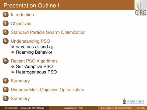
Presentation Outline I1 Introduction
2 Objectives
3 Standard Particle Swarm Optimization
4 Understanding PSOw versus c1 and c2Roaming Behavior
5 Recent PSO AlgorithmsSelf-Adaptive PSOHeterogeneous PSO
6 Summary
7 Dynamic Multi-Objective Optimization
8 Summary
Engelbrecht (University of Pretoria) Advances in PSO IEEE WCCI, 24-29 July 2016 3 / 145
Introduction
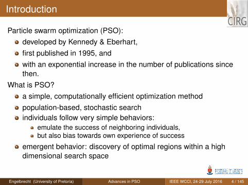
Particle swarm optimization (PSO):developed by Kennedy & Eberhart,first published in 1995, andwith an exponential increase in the number of publications sincethen.
What is PSO?a simple, computationally efficient optimization methodpopulation-based, stochastic searchindividuals follow very simple behaviors:
emulate the success of neighboring individuals,but also bias towards own experience of success
emergent behavior: discovery of optimal regions within a highdimensional search space
Engelbrecht (University of Pretoria) Advances in PSO IEEE WCCI, 24-29 July 2016 4 / 145
Introduction (cont)
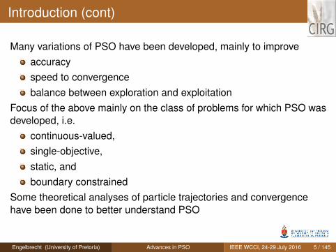
Many variations of PSO have been developed, mainly to improveaccuracyspeed to convergencebalance between exploration and exploitation
Focus of the above mainly on the class of problems for which PSO wasdeveloped, i.e.
continuous-valued,single-objective,static, andboundary constrained
Some theoretical analyses of particle trajectories and convergencehave been done to better understand PSO
Engelbrecht (University of Pretoria) Advances in PSO IEEE WCCI, 24-29 July 2016 5 / 145
Introduction (cont)
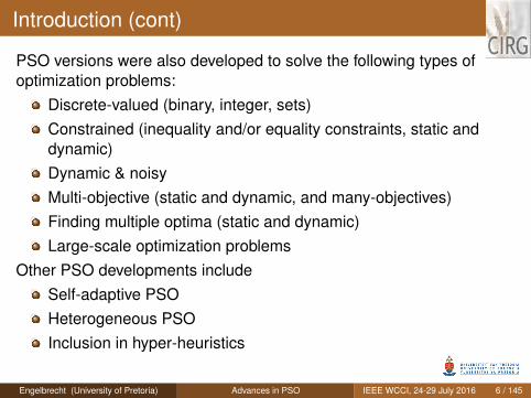
PSO versions were also developed to solve the following types ofoptimization problems:
Discrete-valued (binary, integer, sets)Constrained (inequality and/or equality constraints, static anddynamic)Dynamic & noisyMulti-objective (static and dynamic, and many-objectives)Finding multiple optima (static and dynamic)Large-scale optimization problems
Other PSO developments includeSelf-adaptive PSOHeterogeneous PSOInclusion in hyper-heuristics
Engelbrecht (University of Pretoria) Advances in PSO IEEE WCCI, 24-29 July 2016 6 / 145
Objectives of Tutorial
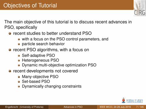
The main objective of this tutorial is to discuss recent advances inPSO, specifically
recent studies to better understand PSOwith a focus on the PSO control parameters, andparticle search behavior
recent PSO algorithms, with a focus onSelf-adaptive PSOHeterogeneous PSODynamic multi-objective optimization PSO
recent developments not coveredMany-objective PSOSet-based PSODynamically changing constraints
Engelbrecht (University of Pretoria) Advances in PSO IEEE WCCI, 24-29 July 2016 7 / 145
Basic Foundations of Particle Swarm OptimizationMain Components
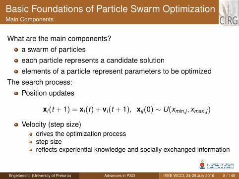
What are the main components?a swarm of particleseach particle represents a candidate solutionelements of a particle represent parameters to be optimized
The search process:Position updates
xi(t + 1) = xi(t) + vi(t + 1), xij(0) ∼ U(xmin,j , xmax ,j)
Velocity (step size)drives the optimization processstep sizereflects experiential knowledge and socially exchanged information
Engelbrecht (University of Pretoria) Advances in PSO IEEE WCCI, 24-29 July 2016 8 / 145
Basic Foundations of Particle Swarm OptimizationSocial Network Structures
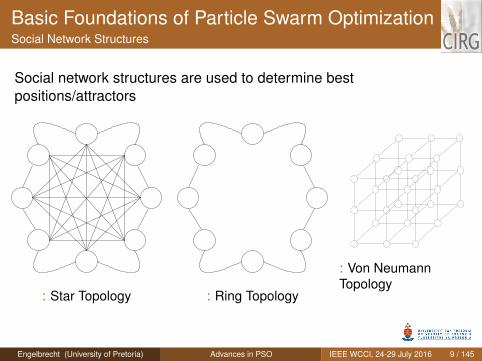
Social network structures are used to determine bestpositions/attractors
: Star Topology : Ring Topology
: Von NeumannTopology
Engelbrecht (University of Pretoria) Advances in PSO IEEE WCCI, 24-29 July 2016 9 / 145
Basic Foundations of Particle Swarm Optimizationglobal best (gbest) PSO
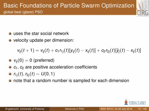
uses the star social networkvelocity update per dimension:
vij(t + 1) = vij(t) + c1r1j(t)[yij(t)− xij(t)] + c2r2j(t)[yj(t)− xij(t)]
vij(0) = 0 (preferred)c1, c2 are positive acceleration coefficientsr1j(t), r2j(t) ∼ U(0,1)
note that a random number is sampled for each dimension
Engelbrecht (University of Pretoria) Advances in PSO IEEE WCCI, 24-29 July 2016 10 / 145
Basic Foundations of Particle Swarm Optimizationgbest PSO (cont)
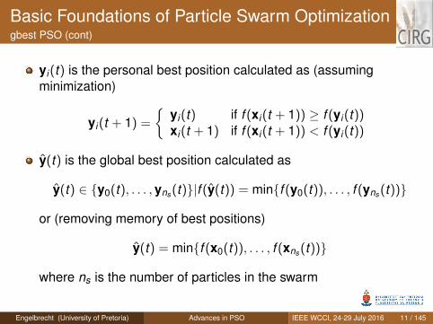
yi(t) is the personal best position calculated as (assumingminimization)
yi(t + 1) =
{yi(t) if f (xi(t + 1)) ≥ f (yi(t))xi(t + 1) if f (xi(t + 1)) < f (yi(t))
y(t) is the global best position calculated as
y(t) ∈ {y0(t), . . . ,yns (t)}|f (y(t)) = min{f (y0(t)), . . . , f (yns (t))}
or (removing memory of best positions)
y(t) = min{f (x0(t)), . . . , f (xns (t))}
where ns is the number of particles in the swarm
Engelbrecht (University of Pretoria) Advances in PSO IEEE WCCI, 24-29 July 2016 11 / 145
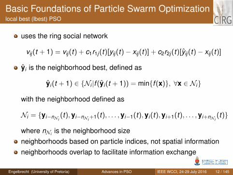
Basic Foundations of Particle Swarm Optimizationlocal best (lbest) PSO
uses the ring social network
vij(t + 1) = vij(t) + c1r1j(t)[yij(t)− xij(t)] + c2r2j(t)[yij(t)− xij(t)]
yi is the neighborhood best, defined as
yi(t + 1) ∈ {Ni |f (yi(t + 1)) = min{f (x)}, ∀x ∈ Ni}
with the neighborhood defined as
Ni = {yi−nNi(t),yi−nNi +1(t), . . . ,yi−1(t),yi(t),yi+1(t), . . . ,yi+nNi
(t)}
where nNi is the neighborhood sizeneighborhoods based on particle indices, not spatial informationneighborhoods overlap to facilitate information exchange
Engelbrecht (University of Pretoria) Advances in PSO IEEE WCCI, 24-29 July 2016 12 / 145
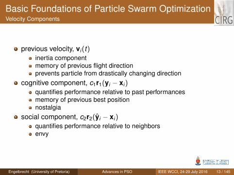
Basic Foundations of Particle Swarm OptimizationVelocity Components
previous velocity, vi(t)inertia componentmemory of previous flight directionprevents particle from drastically changing direction
cognitive component, c1r1(yi − xi)
quantifies performance relative to past performancesmemory of previous best positionnostalgia
social component, c2r2(yi − xi)
quantifies performance relative to neighborsenvy
Engelbrecht (University of Pretoria) Advances in PSO IEEE WCCI, 24-29 July 2016 13 / 145
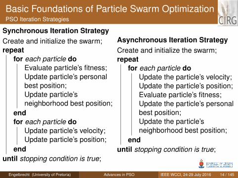
Basic Foundations of Particle Swarm OptimizationPSO Iteration Strategies
Synchronous Iteration StrategyCreate and initialize the swarm;repeat
for each particle doEvaluate particle’s fitness;Update particle’s personalbest position;Update particle’sneighborhood best position;
endfor each particle do
Update particle’s velocity;Update particle’s position;
enduntil stopping condition is true;
Asynchronous Iteration StrategyCreate and initialize the swarm;repeat
for each particle doUpdate the particle’s velocity;Update the particle’s position;Evaluate particle’s fitness;Update the particle’s personalbest position;Update the particle’sneighborhood best position;
enduntil stopping condition is true;
Engelbrecht (University of Pretoria) Advances in PSO IEEE WCCI, 24-29 July 2016 14 / 145
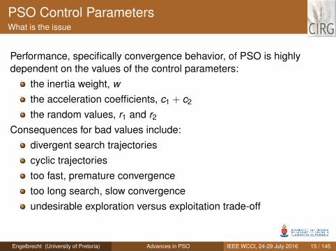
PSO Control ParametersWhat is the issue
Performance, specifically convergence behavior, of PSO is highlydependent on the values of the control parameters:
the inertia weight, wthe acceleration coefficients, c1 + c2
the random values, r1 and r2
Consequences for bad values include:divergent search trajectoriescyclic trajectoriestoo fast, premature convergencetoo long search, slow convergenceundesirable exploration versus exploitation trade-off
Engelbrecht (University of Pretoria) Advances in PSO IEEE WCCI, 24-29 July 2016 15 / 145
PSO Control Parametersr1 and r2
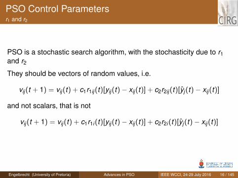
PSO is a stochastic search algorithm, with the stochasticity due to r1and r2
They should be vectors of random values, i.e.
vij(t + 1) = vij(t) + c1r1ij(t)[yij(t)− xij(t)] + c2r2ij(t)[yj(t)− xij(t)]
and not scalars, that is not
vij(t + 1) = vij(t) + c1r1i(t)[yij(t)− xij(t)] + c2r2i(t)[yj(t)− xij(t)]
Engelbrecht (University of Pretoria) Advances in PSO IEEE WCCI, 24-29 July 2016 16 / 145
PSO Control Parametersr1 and r2 (cont)
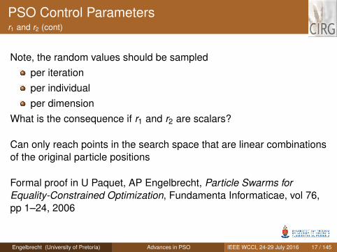
Note, the random values should be sampledper iterationper individualper dimension
What is the consequence if r1 and r2 are scalars?
Can only reach points in the search space that are linear combinationsof the original particle positions
Formal proof in U Paquet, AP Engelbrecht, Particle Swarms forEquality-Constrained Optimization, Fundamenta Informaticae, vol 76,pp 1–24, 2006
Engelbrecht (University of Pretoria) Advances in PSO IEEE WCCI, 24-29 July 2016 17 / 145
PSO Control ParametersEffect of w
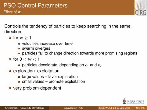
Controls the tendency of particles to keep searching in the samedirection
for w ≥ 1velocities increase over timeswarm divergesparticles fail to change direction towards more promising regions
for 0 < w < 1particles decelerate, depending on c1 and c2
exploration–exploitationlarge values – favor explorationsmall values – promote exploitation
very problem-dependent
Engelbrecht (University of Pretoria) Advances in PSO IEEE WCCI, 24-29 July 2016 18 / 145
PSO Control ParametersEffect of c1 and c2
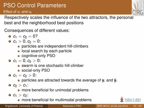
Respectively scales the influence of the two attractors, the personalbest and the neighborhood best positions
Consequences of different values:c1 = c2 = 0?c1 > 0, c2 = 0:
particles are independent hill-climberslocal search by each particlecognitive-only PSO
c1 = 0, c2 > 0:swarm is one stochastic hill-climbersocial-only PSO
c1 = c2 > 0:particles are attracted towards the average of yi and yi
c2 > c1:more beneficial for unimodal problems
c1 > c2:more beneficial for multimodal problems
Engelbrecht (University of Pretoria) Advances in PSO IEEE WCCI, 24-29 July 2016 19 / 145
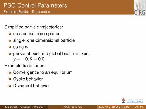
PSO Control ParametersExample Particle Trajectories
Simplified particle trajectories:no stochastic componentsingle, one-dimensional particleusing wpersonal best and global best are fixed:y = 1.0, y = 0.0
Example trajectories:Convergence to an equilibriumCyclic behaviorDivergent behavior
Engelbrecht (University of Pretoria) Advances in PSO IEEE WCCI, 24-29 July 2016 20 / 145

PSO Control ParametersExample Particle Trajectories: Convergent Trajectories
-40
-30
-20
-10
0
10
20
30
0 50 100 150 200 250
xt
t
(a) Time domain
-6e-16
-40 -30 -20 -10 0 10 20 30
im
re
(b) Phase space
: w = 0.5 and φ1 = φ2 = 1.4
Engelbrecht (University of Pretoria) Advances in PSO IEEE WCCI, 24-29 July 2016 21 / 145
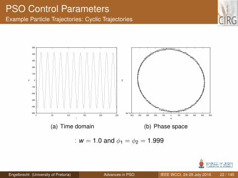
PSO Control ParametersExample Particle Trajectories: Cyclic Trajectories
-500
-400
-300
-200
-100
0
100
200
300
400
500
0 50 100 150 200 250
xt
t
(a) Time domain
-6e-16
-500 -400 -300 -200 -100 0 100 200 300 400 500
im
re
(b) Phase space
: w = 1.0 and φ1 = φ2 = 1.999
Engelbrecht (University of Pretoria) Advances in PSO IEEE WCCI, 24-29 July 2016 22 / 145
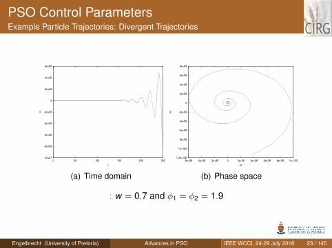
PSO Control ParametersExample Particle Trajectories: Divergent Trajectories
-1e+07
-8e+06
-6e+06
-4e+06
-2e+06
0
2e+06
4e+06
6e+06
0 50 100 150 200 250
xt
t
(a) Time domain
-1.2e+100
-1e+100
-8e+99
-6e+99
-4e+99
-2e+99
0
2e+99
4e+99
6e+99
8e+99
-6e+99 -4e+99 -2e+99 0 2e+99 4e+99 6e+99 8e+99 1e+100
im
re
(b) Phase space
: w = 0.7 and φ1 = φ2 = 1.9
Engelbrecht (University of Pretoria) Advances in PSO IEEE WCCI, 24-29 July 2016 23 / 145
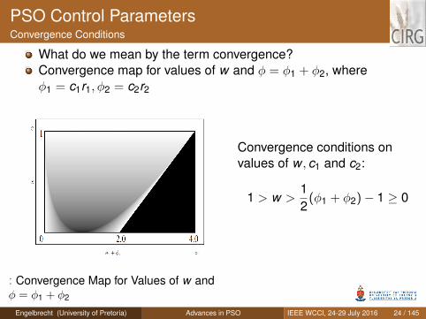
PSO Control ParametersConvergence Conditions
What do we mean by the term convergence?Convergence map for values of w and φ = φ1 + φ2, whereφ1 = c1r1, φ2 = c2r2
: Convergence Map for Values of w andφ = φ1 + φ2
Convergence conditions onvalues of w , c1 and c2:
1 > w >12
(φ1 + φ2)− 1 ≥ 0
Engelbrecht (University of Pretoria) Advances in PSO IEEE WCCI, 24-29 July 2016 24 / 145
PSO Control ParametersStochastic Trajectories
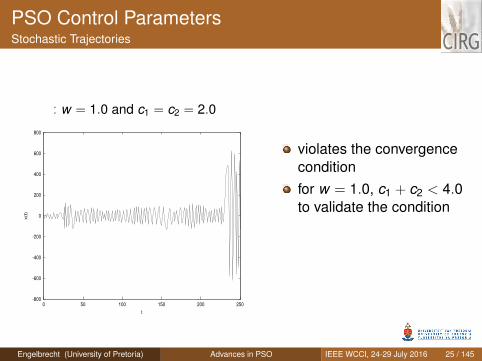
: w = 1.0 and c1 = c2 = 2.0
-800
-600
-400
-200
0
200
400
600
800
0 50 100 150 200 250
x(t
)
t
violates the convergenceconditionfor w = 1.0, c1 + c2 < 4.0to validate the condition
Engelbrecht (University of Pretoria) Advances in PSO IEEE WCCI, 24-29 July 2016 25 / 145
PSO Control ParametersStochastic Trajectories (cont)
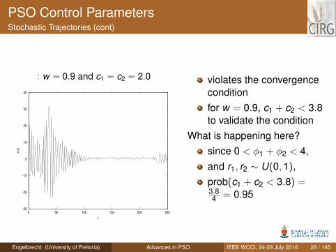
: w = 0.9 and c1 = c2 = 2.0
-30
-20
-10
0
10
20
30
40
0 50 100 150 200 250
x(t
)
t
violates the convergenceconditionfor w = 0.9, c1 + c2 < 3.8to validate the condition
What is happening here?since 0 < φ1 + φ2 < 4,and r1, r2 ∼ U(0,1),prob(c1 + c2 < 3.8) =3.84 = 0.95
Engelbrecht (University of Pretoria) Advances in PSO IEEE WCCI, 24-29 July 2016 26 / 145
PSO Control ParametersStochastic Trajectories (cont)
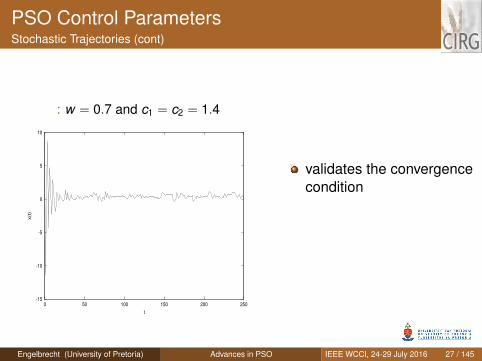
: w = 0.7 and c1 = c2 = 1.4
-15
-10
-5
0
5
10
0 50 100 150 200 250
x(t
)
t
validates the convergencecondition
Engelbrecht (University of Pretoria) Advances in PSO IEEE WCCI, 24-29 July 2016 27 / 145
PSO Control ParametersAlternative Convergence Condition
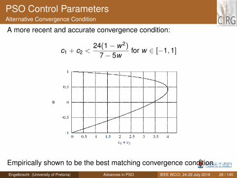
A more recent and accurate convergence condition:
c1 + c2 <24(1− w2)
7− 5wfor w ∈ [−1,1]
Empirically shown to be the best matching convergence conditionEngelbrecht (University of Pretoria) Advances in PSO IEEE WCCI, 24-29 July 2016 28 / 145
PSO Issues: Roaming Particles
Empirical analysis and theoretical proofs showed that particlesleave search boundaries very early during the optimizationprocessPotential problems:
Infeasible solutions: Should better positions be found outside ofboundaries, and no boundary constraint method employed,personal best and neighborhood best positions are pulled outsideof search boundariesWasted search effort: Should better positions not exist outside ofboundaries, particles are eventually pulled back into feasible space.Incorrect swarm diversity calculations: As particles moveoutside of search boundaries, diversity increases
Engelbrecht (University of Pretoria) Advances in PSO IEEE WCCI, 24-29 July 2016 29 / 145
PSO Issues: Roaming ParticlesEmpirical Analysis
Goal of this experiment: Toillustrate
particle roamingbehavior, andinfeasible solutionsmay be found
Experimental setup:A standard gbest PSO was used30 particlesw = 0.729844c1 = c2 = 1.496180Memory-based global best selectionSynchronous position updates50 independent runs for eachinitialization strategy
Engelbrecht (University of Pretoria) Advances in PSO IEEE WCCI, 24-29 July 2016 30 / 145
PSO Issues: Roaming ParticlesBenchmark Functions
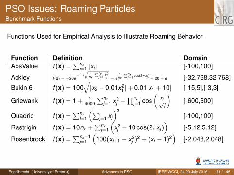
Functions Used for Empirical Analysis to Illustrate Roaming Behavior
Function Definition Domain DimensionAbsValue f (x) =
∑nxj=1 |xi | [-100,100] 30
Ackley f (x) = −20e−0.2
√1
nx∑nx
j=1 x2j − e
1nx∑nx
j=1 cos(2πxj ) + 20 + e [-32.768,32.768] 30
Bukin 6 f (x) = 100√|x2 − 0.01x2
1 |+ 0.01|x1 + 10| [-15,5],[-3,3] 2
Griewank f (x) = 1 + 14000
∑nxj=1 x2
j −∏nx
j=1 cos(
xj√j
)[-600,600] 30
Quadric f (x) =∑nx
l=1
(∑lj=1 xj
)2[-100,100] 30
Rastrigin f (x) = 10nx +∑nx
j=1
(x2
j − 10 cos(2πxj ))
[-5.12,5.12] 30
Rosenbrock f (x) =∑nx−1
j=1
(100(xj+1 − x2
j )2 + (xj − 1)2)
[-2.048,2.048] 30
Engelbrecht (University of Pretoria) Advances in PSO IEEE WCCI, 24-29 July 2016 31 / 145
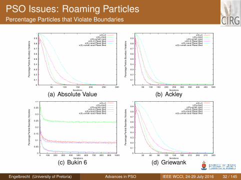
PSO Issues: Roaming ParticlesPercentage Particles that Violate Boundaries
0
0.1
0.2
0.3
0.4
0.5
0.6
0.7
0.8
0.9
1
50 100 150 200 250 300
Perc
enta
ge P
art
icle
Boundary
Vio
latio
ns
Iterations
v(0)=0v(0)=rand
v(0)=small randv(0)=0 Pbest Bnd
v(0)=rand Pbest Bndv(0)=small rand Pbest Bnd
(a) Absolute Value
0
0.1
0.2
0.3
0.4
0.5
0.6
0.7
0.8
0.9
1
50 100 150 200 250 300 350 400 450 500
Perc
enta
ge P
art
icle
Boundary
Vio
latio
ns
Iterations
v(0)=0v(0)=rand
v(0)=small randv(0)=0 Pbest Bnd
v(0)=rand Pbest Bndv(0)=small rand Pbest Bnd
(b) Ackley
0
0.05
0.1
0.15
0.2
0.25
0.3
0.35
0.4
0 100 200 300 400 500 600 700 800 900 1000
Perc
enta
ge P
art
icle
Boundary
Vio
latio
ns
Iterations
v(0)=0v(0)=rand
v(0)=small randv(0)=0 Pbest Bnd
v(0)=rand Pbest Bndv(0)=small rand Pbest Bnd
(c) Bukin 6
0
0.1
0.2
0.3
0.4
0.5
0.6
0.7
0.8
0.9
1
30 60 90 120 150 180 210 240 270 300
Perc
enta
ge P
art
icle
Boundary
Vio
latio
ns
Iterations
v(0)=0v(0)=rand
v(0)=small randv(0)=0 Pbest Bnd
v(0)=rand Pbest Bndv(0)=small rand Pbest Bnd
(d) Griewank
:Engelbrecht (University of Pretoria) Advances in PSO IEEE WCCI, 24-29 July 2016 32 / 145
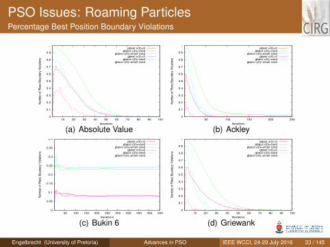
PSO Issues: Roaming ParticlesPercentage Best Position Boundary Violations
0
0.1
0.2
0.3
0.4
0.5
0.6
0.7
0.8
0.9
1
10 20 30 40 50 60 70 80 90 100
Num
ber
of P
best
Boundary
Vio
latio
ns
Iterations
pbest v(0)=0pbest v(0)=rand
pbest v(0)=small randgbest v(0)=0
gbest v(0)=randgbest v(0)=small rand
(a) Absolute Value
0
0.1
0.2
0.3
0.4
0.5
0.6
0.7
0.8
0.9
1
50 100 150 200 250
Num
ber
of P
best
Boundary
Vio
latio
ns
Iterations
pbest v(0)=0pbest v(0)=rand
pbest v(0)=small randgbest v(0)=0
gbest v(0)=randgbest v(0)=small rand
(b) Ackley
0
0.05
0.1
0.15
0.2
0.25
0.3
0.35
0.4
50 100 150 200 250 300 350 400 450 500
Num
ber
of P
best
Boundary
Vio
latio
ns
Iterations
pbest v(0)=0pbest v(0)=rand
pbest v(0)=small randgbest v(0)=0
gbest v(0)=randgbest v(0)=small rand
(c) Bukin 6
0
0.1
0.2
0.3
0.4
0.5
0.6
0.7
0.8
0.9
1
10 20 30 40 50 60 70 80 90 100
Num
ber
of P
best
Boundary
Vio
latio
ns
Iterations
pbest v(0)=0pbest v(0)=rand
pbest v(0)=small randgbest v(0)=0
gbest v(0)=randgbest v(0)=small rand
(d) Griewank
:Engelbrecht (University of Pretoria) Advances in PSO IEEE WCCI, 24-29 July 2016 33 / 145
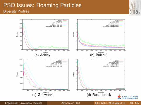
PSO Issues: Roaming ParticlesDiversity Profiles
0
20
40
60
80
100
120
140
80 160 240 320 400 480 560 640 720 800
Div
ers
ity
Iterations
v(0)=0v(0)=rand
v(0)=small randv(0)=0 Pbest Bnd
v(0)=rand Pbest Bndv(0)=small rand Pbest Bnd
(a) Ackley
0
1
2
3
4
5
6
7
0 100 200 300 400 500 600 700 800 900 1000
Div
ers
ity
Iterations
v(0)=0v(0)=rand
v(0)=small randv(0)=0 Pbest Bnd
v(0)=rand Pbest Bndv(0)=small rand Pbest Bnd
(b) Bukin 6
0
500
1000
1500
2000
2500
40 80 120 160 200 240 280 320 360 400
Div
ers
ity
Iterations
v(0)=0v(0)=rand
v(0)=small randv(0)=0 Pbest Bnd
v(0)=rand Pbest Bndv(0)=small rand Pbest Bnd
(c) Griewank
0
1
2
3
4
5
6
7
8
0 100 200 300 400 500 600 700 800 900 1000
Div
ers
ity
Iterations
v(0)=0v(0)=rand
v(0)=small randv(0)=0 Pbest Bnd
v(0)=rand Pbest Bndv(0)=small rand Pbest Bnd
(d) Rosenbrock
:Engelbrecht (University of Pretoria) Advances in PSO IEEE WCCI, 24-29 July 2016 34 / 145
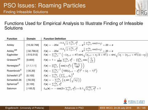
PSO Issues: Roaming ParticlesFinding Infeasible Solutions
Functions Used for Empirical Analysis to Illustrate Finding of InfeasibleSolutions
Function Domain Function Definition
Ackley [10,32.768] f (x) = −20e−0.2
√1n∑nx
j=1 x2j − e
1n∑nx
j=1 cos(2πxj ) + 20 + e
AckleySR [-32.768,0] f (x) = −20e−0.2
√1n∑nx
j=1 z2j − e
1n∑nx
j=1 cos(2πzj ) + 20 + eEggholder [-512,512] f (x) =
∑nx−1j=1
(−(xj+1 + 47) sin(
√|xj+1 + xj/2 + 47|) + sin(
√|xj − (xj+1 + 47)|)(−xj )
)GriewankSR [0,600] f (x) = 1 + 1
4000∑nx
j=1 z2j −
∏nxj=1 cos
(zj√
j
)NorwegianS [-1.1,1.1] f (x) =
∏nxj=1
(cos(πz3
j )
(99+zj
100
))RosenbrockS [-30,30] f (x) =
∑nx−1j=1
(100(zj+1 − z2
j )2 + (zj − 1)2
)Schwefel1.2S [0,100] f (x) =
∑nxj=1
(∑jk=1 zk
)2
Schwefel2.26 [-50,50] f (x) = −∑nx
j=1
(xj sin
(√|xj |))
SphericalS [0,100] f (x) =∑nx
j=1 z2i
Salomon [-100,5] f14(x) = − cos(2π∑nx
j=1 x2j ) + 0.1
√∑nxj=1 x2
j + 1
Engelbrecht (University of Pretoria) Advances in PSO IEEE WCCI, 24-29 July 2016 35 / 145
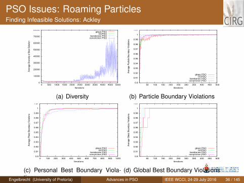
PSO Issues: Roaming ParticlesFinding Infeasible Solutions: Ackley
0
10000
20000
30000
40000
50000
60000
70000
80000
0 500 1000 1500 2000 2500 3000 3500 4000 4500 5000
Ave
rage D
ivers
ity o
f B
est
Solu
tion
Iterations
gbest PSOGCPSO
barebones PSOconstriction PSO
(a) Diversity
0.9
0.91
0.92
0.93
0.94
0.95
0.96
0.97
0.98
0.99
1
1.01
50 100 150 200 250 300 350 400 450 500
Ave
rage P
art
icle
Boundary
Vio
latio
ns
Iterations
gbest PSOGCPSO
barebones PSOconstriction PSO
(b) Particle Boundary Violations
0.9
0.91
0.92
0.93
0.94
0.95
0.96
0.97
0.98
0.99
1
1.01
0 100 200 300 400 500 600 700 800 900 1000
Ave
rage P
best
Boundary
Vio
latio
ns
Iterations
pbest PSOGCPSO
barebones PSOconstriction PSO
(c) Personal Best Boundary Viola-tions
0.9
0.91
0.92
0.93
0.94
0.95
0.96
0.97
0.98
0.99
1
1.01
50 100 150 200 250 300 350 400 450 500
Ave
rage G
best
Boundary
Vio
latio
ns
Iterations
gbest PSOGCPSO
barebones PSOconstriction PSO
(d) Global Best Boundary ViolationsEngelbrecht (University of Pretoria) Advances in PSO IEEE WCCI, 24-29 July 2016 36 / 145
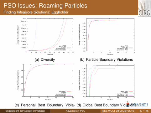
PSO Issues: Roaming ParticlesFinding Infeasible Solutions: Eggholder
0
500000
1e+06
1.5e+06
2e+06
2.5e+06
3e+06
3.5e+06
4e+06
4.5e+06
5e+06
5 10 15 20 25 30 35 40 45 50
Ave
rage D
ivers
ity o
f B
est
Solu
tion
Iterations
gbest PSOGCPSO
barebones PSOconstriction PSO
(a) Diversity
0.8
0.82
0.84
0.86
0.88
0.9
0.92
0.94
0.96
0.98
1
5 10 15 20 25 30
Ave
rage P
art
icle
Boundary
Vio
latio
ns
Iterations
gbest PSOGCPSO
barebones PSOconstriction PSO
(b) Particle Boundary Violations
0
0.2
0.4
0.6
0.8
1
5 10 15 20 25 30
Ave
rage P
best
Boundary
Vio
latio
ns
Iterations
pbest PSOGCPSO
barebones PSOconstriction PSO
(c) Personal Best Boundary Viola-tions
0.8
0.82
0.84
0.86
0.88
0.9
0.92
0.94
0.96
0.98
1
5 10 15 20 25 30
Ave
rage G
best
Boundary
Vio
latio
ns
Iterations
gbest PSOGCPSO
barebones PSOconstriction PSO
(d) Global Best Boundary ViolationsEngelbrecht (University of Pretoria) Advances in PSO IEEE WCCI, 24-29 July 2016 37 / 145
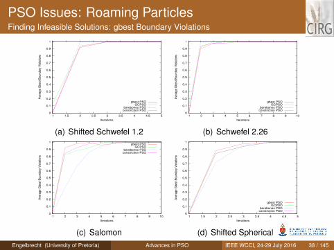
PSO Issues: Roaming ParticlesFinding Infeasible Solutions: gbest Boundary Violations
0
0.1
0.2
0.3
0.4
0.5
0.6
0.7
0.8
0.9
1
1 1.5 2 2.5 3 3.5 4 4.5 5
Ave
rage G
best
Boundary
Vio
latio
ns
Iterations
gbest PSOGCPSO
barebones PSOconstriction PSO
(a) Shifted Schwefel 1.2
0
0.1
0.2
0.3
0.4
0.5
0.6
0.7
0.8
0.9
1
1 2 3 4 5 6 7 8 9 10
Ave
rage G
best
Boundary
Vio
latio
ns
Iterations
gbest PSOGCPSO
barebones PSOconstriction PSO
(b) Schwefel 2.26
0
0.1
0.2
0.3
0.4
0.5
0.6
0.7
0.8
0.9
1
1 2 3 4 5 6 7 8 9 10
Ave
rage G
best
Boundary
Vio
latio
ns
Iterations
gbest PSOGCPSO
barebones PSOconstriction PSO
(c) Salomon
0
0.1
0.2
0.3
0.4
0.5
0.6
0.7
0.8
0.9
1
1 1.5 2 2.5 3 3.5 4 4.5 5
Ave
rage G
best
Boundary
Vio
latio
ns
Iterations
gbest PSOGCPSO
barebones PSOconstriction PSO
(d) Shifted SphericalEngelbrecht (University of Pretoria) Advances in PSO IEEE WCCI, 24-29 July 2016 38 / 145
PSO Issues: Roaming ParticlesSolving the Problem
The roaming problem can be addressed byusing boundary constraint mechanismsupdate personal best positions only when solution qualityimproves AND the particle is feasible (within bounds)
However, note that some problems do not have boundary constraints,such as neural network training...
Engelbrecht (University of Pretoria) Advances in PSO IEEE WCCI, 24-29 July 2016 39 / 145
Self-Adaptive Particle Swarm OptimizationIntroduction
PSO performance is very sensitive to control parameter valuesApproaches to find the best values for control parameters:
Just use the values published in literature?Do you want something that works,or something that works best?
Fine-tuned static valuesDynamically changing valuesSelf-adaptive control parameters
Engelbrecht (University of Pretoria) Advances in PSO IEEE WCCI, 24-29 July 2016 40 / 145
Self-Adaptive Particle Swarm OptimizationControl Parameter Tuning
Factorial designF-RaceControl parameter dependenciesProblem dependencyComputationally expensive
Engelbrecht (University of Pretoria) Advances in PSO IEEE WCCI, 24-29 July 2016 41 / 145
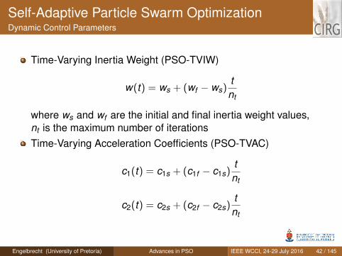
Self-Adaptive Particle Swarm OptimizationDynamic Control Parameters
Time-Varying Inertia Weight (PSO-TVIW)
w(t) = ws + (wf − ws)tnt
where ws and wf are the initial and final inertia weight values,nt is the maximum number of iterationsTime-Varying Acceleration Coefficients (PSO-TVAC)
c1(t) = c1s + (c1f − c1s)tnt
c2(t) = c2s + (c2f − c2s)tnt
Engelbrecht (University of Pretoria) Advances in PSO IEEE WCCI, 24-29 July 2016 42 / 145
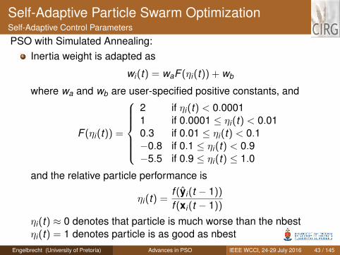
Self-Adaptive Particle Swarm OptimizationSelf-Adaptive Control Parameters
PSO with Simulated Annealing:Inertia weight is adapted as
wi(t) = waF (ηi(t)) + wb
where wa and wb are user-specified positive constants, and
F (ηi(t)) =
2 if ηi(t) < 0.00011 if 0.0001 ≤ ηi(t) < 0.010.3 if 0.01 ≤ ηi(t) < 0.1−0.8 if 0.1 ≤ ηi(t) < 0.9−5.5 if 0.9 ≤ ηi(t) ≤ 1.0
and the relative particle performance is
ηi(t) =f (yi(t − 1))
f (xi(t − 1))
ηi(t) ≈ 0 denotes that particle is much worse than the nbestηi(t) = 1 denotes particle is as good as nbest
Engelbrecht (University of Pretoria) Advances in PSO IEEE WCCI, 24-29 July 2016 43 / 145
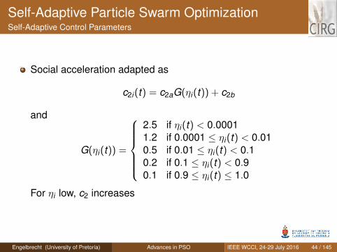
Self-Adaptive Particle Swarm OptimizationSelf-Adaptive Control Parameters
Social acceleration adapted as
c2i(t) = c2aG(ηi(t)) + c2b
and
G(ηi(t)) =
2.5 if ηi(t) < 0.00011.2 if 0.0001 ≤ ηi(t) < 0.010.5 if 0.01 ≤ ηi(t) < 0.10.2 if 0.1 ≤ ηi(t) < 0.90.1 if 0.9 ≤ ηi(t) ≤ 1.0
For ηi low, c2 increases
Engelbrecht (University of Pretoria) Advances in PSO IEEE WCCI, 24-29 July 2016 44 / 145
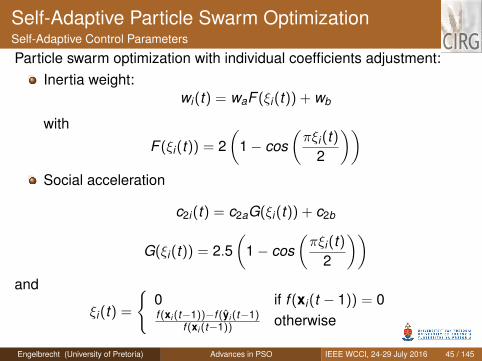
Self-Adaptive Particle Swarm OptimizationSelf-Adaptive Control Parameters
Particle swarm optimization with individual coefficients adjustment:Inertia weight:
wi(t) = waF (ξi(t)) + wb
with
F (ξi(t)) = 2(
1− cos(πξi(t)
2
))Social acceleration
c2i(t) = c2aG(ξi(t)) + c2b
G(ξi(t)) = 2.5(
1− cos(πξi(t)
2
))and
ξi(t) =
{0 if f (xi(t − 1)) = 0f (xi (t−1))−f (yi (t−1)
f (xi (t−1)) otherwise
Engelbrecht (University of Pretoria) Advances in PSO IEEE WCCI, 24-29 July 2016 45 / 145
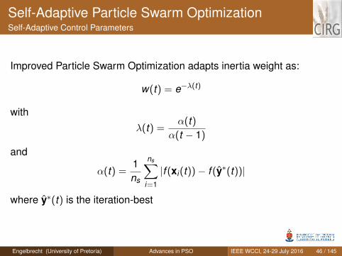
Self-Adaptive Particle Swarm OptimizationSelf-Adaptive Control Parameters
Improved Particle Swarm Optimization adapts inertia weight as:
w(t) = e−λ(t)
withλ(t) =
α(t)α(t − 1)
and
α(t) =1ns
ns∑i=1
|f (xi(t))− f (y∗(t))|
where y∗(t) is the iteration-best
Engelbrecht (University of Pretoria) Advances in PSO IEEE WCCI, 24-29 July 2016 46 / 145
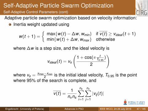
Self-Adaptive Particle Swarm OptimizationSelf-Adaptive Control Parameters (cont)
Adaptive particle swarm optimization based on velocity information:Inertia weight updated using
w(t + 1) =
{max{w(t)−∆w ,wmin} if v(t) ≥ videal(t + 1)min{w(t) + ∆w ,wmax} otherwise
where ∆w is a step size, and the ideal velocity is
videal(t) = vs
(1 + cos(π t
T0.95)
2
)
where vs = xmax−xmin2 is the initial ideal velocity, T0.95 is the point
where 95% of the search is complete, and
v(t) =1
nxns
ns∑i=1
nx∑j=1
|vij(t)|
Engelbrecht (University of Pretoria) Advances in PSO IEEE WCCI, 24-29 July 2016 47 / 145
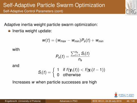
Self-Adaptive Particle Swarm OptimizationSelf-Adaptive Control Parameters (cont)
Adaptive inertia weight particle swarm optimization:Inertia weight update:
w(t) = (wmax − wmin)Ps(t) + wmin
with
Ps(t) =
∑nsi=1 Si(t)
ns
and
Si(t) =
{1 if f (yi(t)) < f (yi(t − 1))0 otherwise
Increases w when particle successes are high
Engelbrecht (University of Pretoria) Advances in PSO IEEE WCCI, 24-29 July 2016 48 / 145
Self-Adaptive Particle Swarm OptimizationSelf-Adaptive Control Parameters (cont)
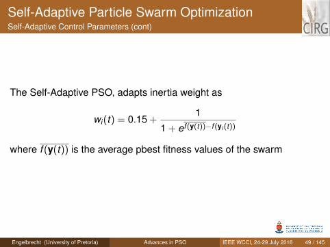
The Self-Adaptive PSO, adapts inertia weight as
wi(t) = 0.15 +1
1 + ef (y(t))−f (yi (t))
where f (y(t)) is the average pbest fitness values of the swarm
Engelbrecht (University of Pretoria) Advances in PSO IEEE WCCI, 24-29 July 2016 49 / 145
Self-Adaptive Particle Swarm OptimizationSummary
Issues with current self-adaptive approaches:Most, at some point in time, violate convergence conditionsConverge prematurely, with little exploration of control parameterspaceIntroduce more control parameters
Engelbrecht (University of Pretoria) Advances in PSO IEEE WCCI, 24-29 July 2016 50 / 145
Heterogeneous Particle Swarm OptimizationIntroduction
Particles in standard particle swarm optimization (PSO), and most ofits modifications, follow the same behavior:
particles implement the same velocity and position update rulesparticles therefore exhibit the same search behavioursthe same exploration and explotation abilities are achieved
Heterogeneous swarms contain particles that follow differentbehaviors:
particles follow different velocity and position update rulessome particles may explore longer than others, while some mayexploit earlier than othersa better balance of exploration and exploitation can be achievedprovided a pool of different behaviors is used
Akin to hyper-heuristics, ensemble methods, multi-methods
Engelbrecht (University of Pretoria) Advances in PSO IEEE WCCI, 24-29 July 2016 51 / 145
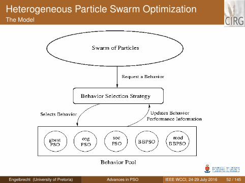
Heterogeneous Particle Swarm OptimizationThe Model
Engelbrecht (University of Pretoria) Advances in PSO IEEE WCCI, 24-29 July 2016 52 / 145
Heterogeneous Particle Swarm OptimizationAbout Behaviors
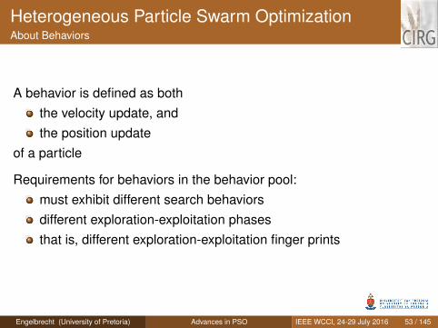
A behavior is defined as boththe velocity update, andthe position update
of a particle
Requirements for behaviors in the behavior pool:must exhibit different search behaviorsdifferent exploration-exploitation phasesthat is, different exploration-exploitation finger prints
Engelbrecht (University of Pretoria) Advances in PSO IEEE WCCI, 24-29 July 2016 53 / 145
Heterogeneous Particle Swarm OptimizationExploration-Exploitation Finger Prints
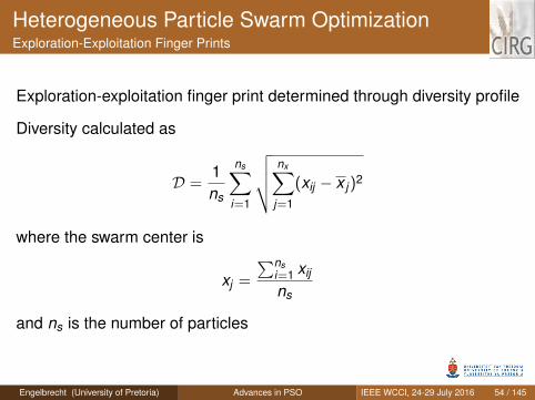
Exploration-exploitation finger print determined through diversity profile
Diversity calculated as
D =1ns
ns∑i=1
√√√√ nx∑j=1
(xij − x j)2
where the swarm center is
xj =
∑nsi=1 xij
ns
and ns is the number of particles
Engelbrecht (University of Pretoria) Advances in PSO IEEE WCCI, 24-29 July 2016 54 / 145
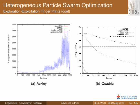
Heterogeneous Particle Swarm OptimizationExploration-Exploitation Finger Prints (cont)
0
10000
20000
30000
40000
50000
60000
70000
80000
0 500 1000 1500 2000 2500 3000 3500 4000 4500 5000
Ave
rag
e D
ive
rsity o
f B
est
So
lutio
n
Iterations
gbest PSOGCPSO
barebones PSOconstriction PSO
(a) Ackley (b) Quadric
Engelbrecht (University of Pretoria) Advances in PSO IEEE WCCI, 24-29 July 2016 55 / 145
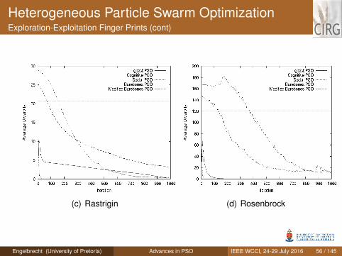
Heterogeneous Particle Swarm OptimizationExploration-Exploitation Finger Prints (cont)
(c) Rastrigin (d) Rosenbrock
Engelbrecht (University of Pretoria) Advances in PSO IEEE WCCI, 24-29 July 2016 56 / 145
Heterogeneous Particle Swarm OptimizationReview
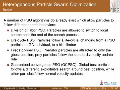
A number of PSO algorithms do already exist which allow particles tofollow different search behaviors:
Division of labor PSO: Particles are allowed to switch to localsearch near the end of the search processLife-cycle PSO: Particles follow a life-cycle, changing from a PSOparticle, to GA individual, to a hill-climberPredator-prey PSO: Predator particles are attracted to only thegbest position, prey particles follow the standard velocity updateruleGuaranteed convergence PSO (GCPSO): Global best particlefollows a different, exploitaitve search around best position, whileother particles follow normal velocity updates
Engelbrecht (University of Pretoria) Advances in PSO IEEE WCCI, 24-29 July 2016 57 / 145
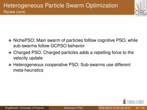
Heterogeneous Particle Swarm OptimizationReview (cont)
NichePSO: Main swarm of particles folllow cognitive PSO, whilesub-swarms follow GCPSO behaviorCharged PSO: Charged particles adds a repelling force to thevelocity updateHeterogeneous cooperative PSO: Sub-swarms use differentmeta-heuristics
Engelbrecht (University of Pretoria) Advances in PSO IEEE WCCI, 24-29 July 2016 58 / 145
Heterogeneous Particle Swarm OptimizationTwo HPSO Models
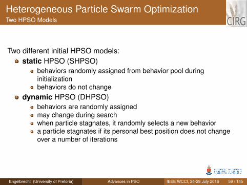
Two different initial HPSO models:static HPSO (SHPSO)
behaviors randomly assigned from behavior pool duringinitializationbehaviors do not change
dynamic HPSO (DHPSO)behaviors are randomly assignedmay change during searchwhen particle stagnates, it randomly selects a new behaviora particle stagnates if its personal best position does not changeover a number of iterations
Engelbrecht (University of Pretoria) Advances in PSO IEEE WCCI, 24-29 July 2016 59 / 145
Heterogeneous Particle Swarm OptimizationSelf-Adaptive HPSO
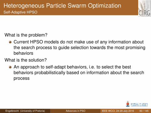
What is the problem?Current HPSO models do not make use of any information aboutthe search process to guide selection towards the most promisingbehaviors
What is the solution?An approach to self-adapt behaviors, i.e. to select the bestbehaviors probabilistically based on information about the searchprocess
Engelbrecht (University of Pretoria) Advances in PSO IEEE WCCI, 24-29 July 2016 60 / 145
Heterogeneous Particle Swarm OptimizationSelf-Adaptive HPSO: Review
Related self-adaptive approaches to HPSO algorithms:Difference proportional probability PSO (DPP-PSO)
particle behaviors change to the nbest particle behaviorbased on probability proportional to how much better the nbestparticle isincludes static particles for each behavior, i.e. behaviors do notchangeonly two behaviors, i.e. FIPS and original PSO
Adaptive learning PSO-II (ALPSO-II)Behaviors are selected probabilistically based on improvementsthat they affect to the quality of the corresponding particlesOverly complex and computationally expensive
Engelbrecht (University of Pretoria) Advances in PSO IEEE WCCI, 24-29 July 2016 61 / 145
Heterogeneous Particle Swarm OptimizationSelf-Adaptive HPSO: General Structure
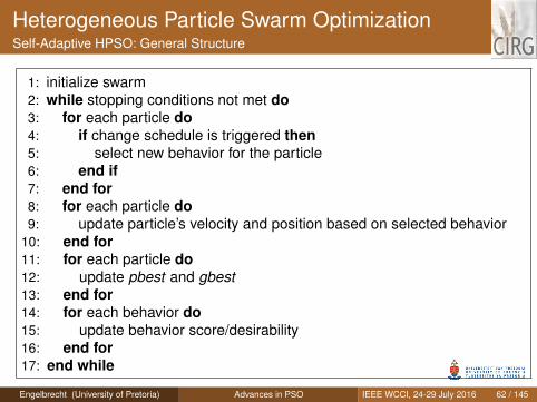
1: initialize swarm2: while stopping conditions not met do3: for each particle do4: if change schedule is triggered then5: select new behavior for the particle6: end if7: end for8: for each particle do9: update particle’s velocity and position based on selected behavior
10: end for11: for each particle do12: update pbest and gbest13: end for14: for each behavior do15: update behavior score/desirability16: end for17: end while
Engelbrecht (University of Pretoria) Advances in PSO IEEE WCCI, 24-29 July 2016 62 / 145
Heterogeneous Particle Swarm OptimizationSelf-Adaptive HPSO: Pheromone-Based
Expanded behavior pool: That of dHPSO, plusQuantum PSO (QPSO)Time-varying inertia weight PSO (TVIW-PSO)Time-varying acceleration coefficients (TVAC-PSO)Fully informed particle swarm (FIPS)
Two self-adaptive strategies inspired by foraging behavior of antsAnts are able to find the shortest path between their nest and afood sourcePaths are followed probabilistically based on pheromoneconcentrations on the paths
Engelbrecht (University of Pretoria) Advances in PSO IEEE WCCI, 24-29 July 2016 63 / 145

Heterogeneous Particle Swarm OptimizationSelf-Adaptive HPSO: Pheromone-Based (cont)
Definitions:B is the total number of behaviorsb is a behavior indexpb is the pheronome concentration for behavior bprobb(t) is the probability of selecting behavior b at time step t
probb(t) =pb(t)∑Bi=1 pi(t)
Each particle selects a new behavior, using Roulette wheel selection,when a behavior change is triggered
Engelbrecht (University of Pretoria) Advances in PSO IEEE WCCI, 24-29 July 2016 64 / 145
Heterogeneous Particle Swarm OptimizationSelf-Adaptive HPSO: Pheromone-Based (cont)
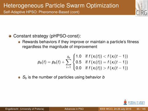
Constant strategy (pHPSO-const):Rewards behaviors if they improve or maintain a particle’s fitnessregardless the magnitude of improvement
pb(t) = pb(t) +
Sb∑i=1
1.0 if f (xi (t)) < f (xi (t − 1))
0.5 if f (xi (t)) = f (xi (t − 1))
0.0 if f (xi (t)) > f (xi (t − 1))
Sb is the number of particles using behavior b
Engelbrecht (University of Pretoria) Advances in PSO IEEE WCCI, 24-29 July 2016 65 / 145
Heterogeneous Particle Swarm OptimizationSelf-Adaptive HPSO: Pheromone-Based (cont)
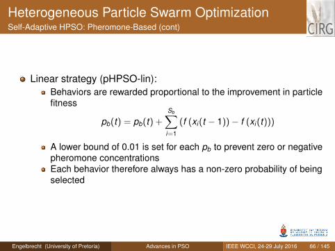
Linear strategy (pHPSO-lin):Behaviors are rewarded proportional to the improvement in particlefitness
pb(t) = pb(t) +
Sb∑i=1
(f (xi (t − 1))− f (xi (t)))
A lower bound of 0.01 is set for each pb to prevent zero or negativepheromone concentrationsEach behavior therefore always has a non-zero probability of beingselected
Engelbrecht (University of Pretoria) Advances in PSO IEEE WCCI, 24-29 July 2016 66 / 145
Heterogeneous Particle Swarm OptimizationSelf-Adaptive HPSO: Pheromone-Based (cont)
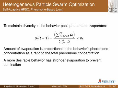
To maintain diversity in the behavior pool, pheromone evaporates:
pb(t + 1) =
(∑Bi=1,i 6=b pi
)∑B
i=1 pi× pb
Amount of evaporation is proportional to the behavior’s pheromoneconcentration as a ratio to the total pheromone concentration
A more desirable behavior has stronger evaporation to preventdomination
Engelbrecht (University of Pretoria) Advances in PSO IEEE WCCI, 24-29 July 2016 67 / 145
Heterogeneous Particle Swarm OptimizationSelf-Adaptive HPSO: Pheromone-Based (cont)
The pHPSO strategies arecomputationally less expensive than others,behaviors are self-adapted based on success of thecorresponding behaviors, andbetter exploration of behavior space is achieved throughpheromone evaporationintroduces no new control parameters
Engelbrecht (University of Pretoria) Advances in PSO IEEE WCCI, 24-29 July 2016 68 / 145
Heterogeneous Particle Swarm OptimizationSelf-Adaptive HPSO: Frequency-Based
Frequency-based HPSO is based on the premise that behaviors aremore desirable if they frequently perform well:
Each behavior has a success counterSuccess counter keeps track of the number of times that thebehavior improved the fitness of a particleOnly the successes of the previous k iterations are considered, sothat behaviors that performed well initially, and bad later, do notcontinue to dominate in the selection processBehaviors change when a particle’s pbest position stagnatesNext behavior chosen using tournament selectionTwo new control parameters: k and tournament size
Engelbrecht (University of Pretoria) Advances in PSO IEEE WCCI, 24-29 July 2016 69 / 145
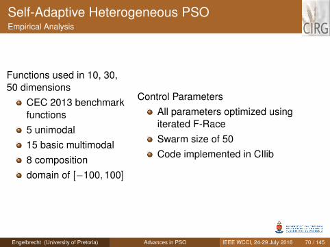
Self-Adaptive Heterogeneous PSOEmpirical Analysis
Functions used in 10, 30,50 dimensions
CEC 2013 benchmarkfunctions5 unimodal15 basic multimodal8 compositiondomain of [−100,100]
Control ParametersAll parameters optimized usingiterated F-RaceSwarm size of 50Code implemented in CIlib
Engelbrecht (University of Pretoria) Advances in PSO IEEE WCCI, 24-29 July 2016 70 / 145
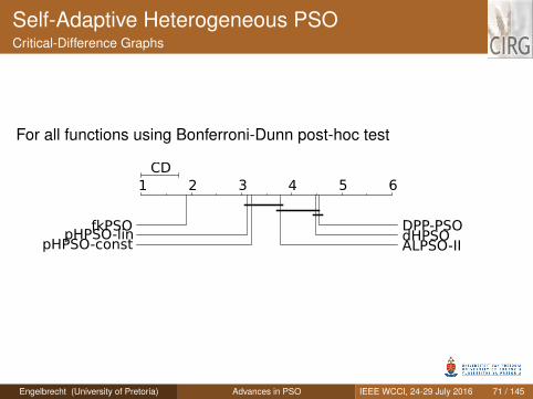
Self-Adaptive Heterogeneous PSOCritical-Difference Graphs
For all functions using Bonferroni-Dunn post-hoc test
Engelbrecht (University of Pretoria) Advances in PSO IEEE WCCI, 24-29 July 2016 71 / 145

Self-Adaptive Heterogeneous PSOCritical-Difference Graphs
For unimodal functions using Bonferroni-Dunn post-hoc test
Engelbrecht (University of Pretoria) Advances in PSO IEEE WCCI, 24-29 July 2016 72 / 145
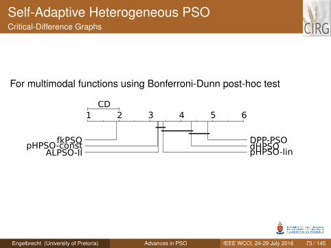
Self-Adaptive Heterogeneous PSOCritical-Difference Graphs
For multimodal functions using Bonferroni-Dunn post-hoc test
Engelbrecht (University of Pretoria) Advances in PSO IEEE WCCI, 24-29 July 2016 73 / 145
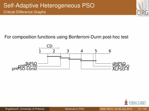
Self-Adaptive Heterogeneous PSOCritical-Difference Graphs
For composition functions using Bonferroni-Dunn post-hoc test
Engelbrecht (University of Pretoria) Advances in PSO IEEE WCCI, 24-29 July 2016 74 / 145
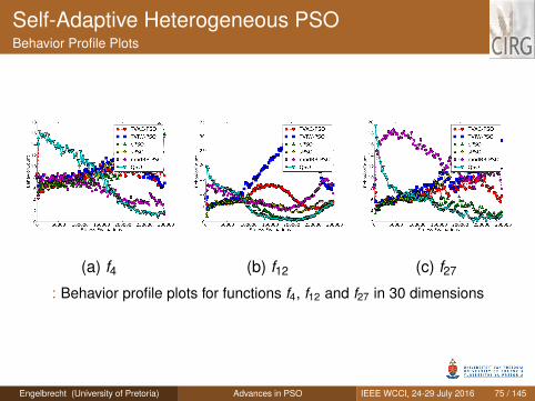
Self-Adaptive Heterogeneous PSOBehavior Profile Plots
(a) f4 (b) f12 (c) f27
: Behavior profile plots for functions f4, f12 and f27 in 30 dimensions
Engelbrecht (University of Pretoria) Advances in PSO IEEE WCCI, 24-29 July 2016 75 / 145
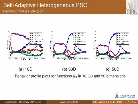
Self-Adaptive Heterogeneous PSOBehavior Profile Plots (cont)
(a) 10D (b) 30D (c) 50D
: Behavior profile plots for functions f10 in 10, 30 and 50 dimensions
Engelbrecht (University of Pretoria) Advances in PSO IEEE WCCI, 24-29 July 2016 76 / 145
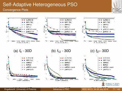
Self-Adaptive Heterogeneous PSOConvergence Plots
(a) f4 - 30D (b) f12 - 30D (c) f27- 30D
(d) f10 - 10D (e) f10 - 30D (f) f10- 50DEngelbrecht (University of Pretoria) Advances in PSO IEEE WCCI, 24-29 July 2016 77 / 145
Self-Adaptive Heterogeneous PSOBehavior Changing Schedules
What is the issue?Particles should be allowed to change their behavior during thesearch processChange should occur when the behavior no longer contribute toimproving solution quality
Current approaches:Select at every iterationSelect when pbest position stagnates over a number of iterations
Engelbrecht (University of Pretoria) Advances in PSO IEEE WCCI, 24-29 July 2016 78 / 145
Self-Adaptive Heterogeneous PSOBehavior Changing Schedules (cont)
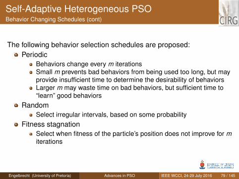
The following behavior selection schedules are proposed:Periodic
Behaviors change every m iterationsSmall m prevents bad behaviors from being used too long, but mayprovide insufficient time to determine the desirability of behaviorsLarger m may waste time on bad behaviors, but sufficient time to“learn” good behaviors
RandomSelect irregular intervals, based on some probability
Fitness stagnationSelect when fitness of the particle’s position does not improve for miterations
Engelbrecht (University of Pretoria) Advances in PSO IEEE WCCI, 24-29 July 2016 79 / 145
Self-Adaptive Heterogeneous PSOResetting Strategies
The following particle state resetting strategies are considered:No resetting of velocity and personal best positionReset velocity upon behavior change to random valuePersonal best reset, which sets particle to its pbest position afterbehavior changeReset both velocity and personal best
Engelbrecht (University of Pretoria) Advances in PSO IEEE WCCI, 24-29 July 2016 80 / 145
Self-Adaptive Heterogeneous PSOResetting Strategies (cont)
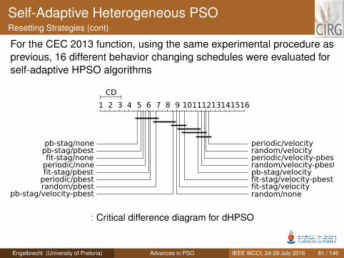
For the CEC 2013 function, using the same experimental procedure asprevious, 16 different behavior changing schedules were evaluated forself-adaptive HPSO algorithms
: Critical difference diagram for dHPSO
Engelbrecht (University of Pretoria) Advances in PSO IEEE WCCI, 24-29 July 2016 81 / 145
Self-Adaptive Heterogeneous PSOResetting Strategies (cont)
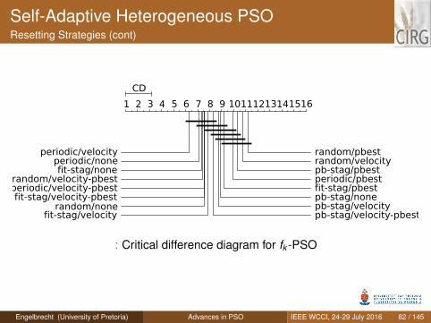
: Critical difference diagram for fk -PSO
Engelbrecht (University of Pretoria) Advances in PSO IEEE WCCI, 24-29 July 2016 82 / 145
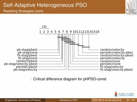
Self-Adaptive Heterogeneous PSOResetting Strategies (cont)
: Critical difference diagram for pHPSO-const
Engelbrecht (University of Pretoria) Advances in PSO IEEE WCCI, 24-29 July 2016 83 / 145
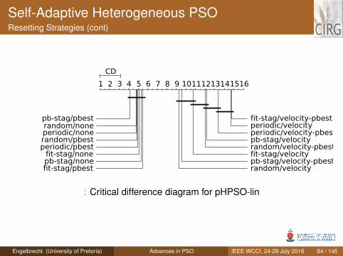
Self-Adaptive Heterogeneous PSOResetting Strategies (cont)
: Critical difference diagram for pHPSO-lin
Engelbrecht (University of Pretoria) Advances in PSO IEEE WCCI, 24-29 July 2016 84 / 145
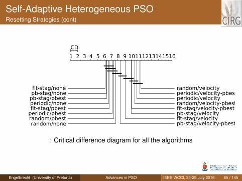
Self-Adaptive Heterogeneous PSOResetting Strategies (cont)
: Critical difference diagram for all the algorithms
Engelbrecht (University of Pretoria) Advances in PSO IEEE WCCI, 24-29 July 2016 85 / 145
Summary
While the original PSO and most of its variants force all particlesto follow the same behavior, different PSO variants show differentsearch behaviorsHeterogeneous PSO (HPSO) algorithms allow different particlesto follow different search behaviorsProposed the following HPSO strategies:
Static HPSO: Behaviors randomly assigned upon initialization anddo no changeDynamic HPSO: Behaviors randomly selected when pbest positionstagnatesSelf-Adaptive HPSO:
Pheromone-based strategies, where probability of being selected isproportional to successFrequency-based strategy, where behaviors are selected based onfrequency of improving particle fitness
Engelbrecht (University of Pretoria) Advances in PSO IEEE WCCI, 24-29 July 2016 86 / 145
Summary
sHPSO and dHPSO improve performance significantly incomparison with the individual behaviorssHPSO and dHPSO are highly scalable compared to individualbehaviorspHPSO and fk -HPSO perform better than other HPSO algorithms,with fk -HPSO performing bestSelf-adaptive HPSO strategies show clearly how differentbehaviors are preferred at different points during the searchprocessProposed self-adaptive HPSO strategies are computationally lesscomplex than other HPSO strategiesBehavior changing schedules have been shown to have an effecton performance
Engelbrecht (University of Pretoria) Advances in PSO IEEE WCCI, 24-29 July 2016 87 / 145
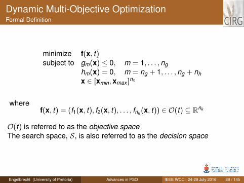
Dynamic Multi-Objective OptimizationFormal Definition
minimize f(x, t)subject to gm(x) ≤ 0, m = 1, . . . ,ng
hm(x) = 0, m = ng + 1, . . . ,ng + nhx ∈ [xmin,xmax ]nx
wheref(x, t) = (f1(x, t), f2(x, t), . . . , fnk (x, t)) ∈ O(t) ⊆ Rnk
O(t) is referred to as the objective spaceThe search space, S, is also referred to as the decision space
Engelbrecht (University of Pretoria) Advances in PSO IEEE WCCI, 24-29 July 2016 88 / 145
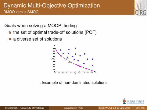
Dynamic Multi-Objective OptimizationDMOO versus SMOO
Goals when solving a MOOP: findingthe set of optimal trade-off solutions (POF)a diverse set of solutions
: Example of non-dominated solutions
Engelbrecht (University of Pretoria) Advances in PSO IEEE WCCI, 24-29 July 2016 89 / 145
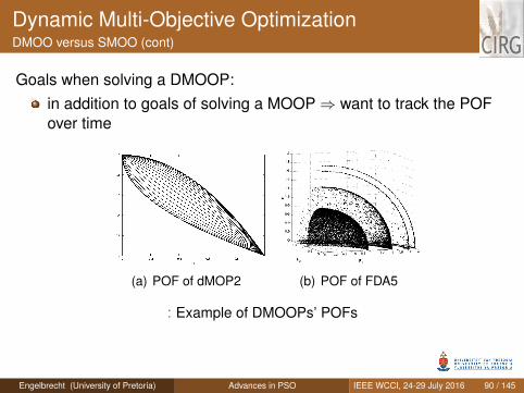
Dynamic Multi-Objective OptimizationDMOO versus SMOO (cont)
Goals when solving a DMOOP:in addition to goals of solving a MOOP⇒ want to track the POFover time
(a) POF of dMOP2 (b) POF of FDA5
: Example of DMOOPs’ POFs
Engelbrecht (University of Pretoria) Advances in PSO IEEE WCCI, 24-29 July 2016 90 / 145
Dynamic Multi-Objective OptimizationThe Main Gaps
The following gaps are identified in DMOO literature:Most research in MOO was done on static multi-objectiveoptimization problems (SMOOPs) and dynamic single-objectiveoptimization problems (DSOOPs)Even though PSO successfully solved both SMOOPs andDSOOPs
Mostly evolutionary algorithms (EAs) were developed to solveDMOOPsLess than a handful of PSOs were developed for DMOO
For DMOO, there is a lack of standardbenchmark functions, andperformance measures
⇒ Difficult to evaluate and compare dynamic multi-objectiveoptimization algorithms (DMOAs)
Engelbrecht (University of Pretoria) Advances in PSO IEEE WCCI, 24-29 July 2016 91 / 145
Dynamic Multi-Objective OptimizationBenchmark Functions
An ideal MOO (static or dynamic) set of benchmark functions shouldTest for difficulties to converge towards the Pareto-optimal front(POF)
MultimodalityThere are many POFsThe algorithm may become stuck on a local POF
Deception (@)There are at least to POFsThe algorithm is "tricked" into converging on the local POF
Isolated optimum (@)Fitness landscape have flat regionsIn such regions, small perturbations in decisionvariables do notchange objective function valuesThere is very little useful information to guide the search towards aPOF
Engelbrecht (University of Pretoria) Advances in PSO IEEE WCCI, 24-29 July 2016 92 / 145
Dynamic Multi-Objective OptimizationBenchmark Functions (cont)
Different shapes of POFsConvexity or non-convexity in the POFDiscontinuous POF, i.e. disconnected sub-regions that arecontinuous (@)Non-uniform distribution of solutions in the POF
Have various types or shapes of Pareto-optimal set (POS) (@)Have decision variables with dependencies or linkages
Engelbrecht (University of Pretoria) Advances in PSO IEEE WCCI, 24-29 July 2016 93 / 145
Dynamic Multi-Objective OptimizationBenchmark Functions (cont)
An ideal DMOOP benchmark function suite should include problemswith the following characteristics:
Solutions in the POF that over time may become dominatedStatic POF shape, but its location in decision space changesDistribution of solutions changes over timeThe shape of the POFs should change over time:
from convex to non-convex or vice versafrom continuous to disconnected or vice versa
Have decision variables with different rates of change over timeInclude cases where the POF depends on the values of previousPOSs or POFsEnable changing the number of decision variables over timeEnable changing the number of objective functions over time
Engelbrecht (University of Pretoria) Advances in PSO IEEE WCCI, 24-29 July 2016 94 / 145
Dynamic Multi-Objective OptimizationBenchmark Functions (cont)
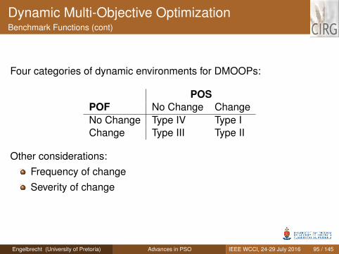
Four categories of dynamic environments for DMOOPs:
POSPOF No Change ChangeNo Change Type IV Type IChange Type III Type II
Other considerations:Frequency of changeSeverity of change
Engelbrecht (University of Pretoria) Advances in PSO IEEE WCCI, 24-29 July 2016 95 / 145
Dynamic Multi-Objective OptimizationBenchmark Functions (cont)
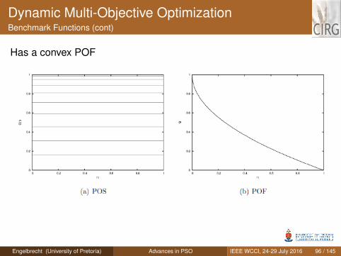
Has a convex POF
Engelbrecht (University of Pretoria) Advances in PSO IEEE WCCI, 24-29 July 2016 96 / 145
Dynamic Multi-Objective OptimizationBenchmark Functions (cont)
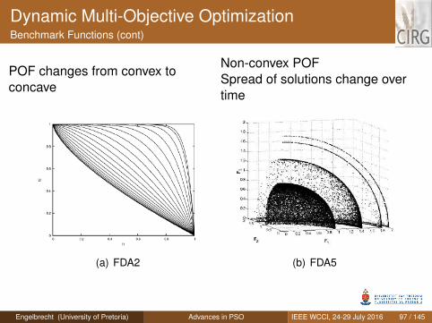
POF changes from convex toconcave
Non-convex POFSpread of solutions change overtime
(a) FDA2 (b) FDA5
Engelbrecht (University of Pretoria) Advances in PSO IEEE WCCI, 24-29 July 2016 97 / 145
Dynamic Multi-Objective OptimizationBenchmark Functions (cont)
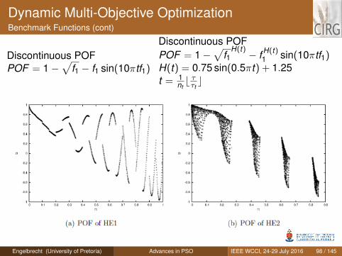
Discontinuous POFPOF = 1−
√f1 − f1 sin(10πtf1)
Discontinuous POFPOF = 1−
√f1
H(t) − f H(t)1 sin(10πtf1)
H(t) = 0.75 sin(0.5πt) + 1.25t = 1
ntb ττtc
Engelbrecht (University of Pretoria) Advances in PSO IEEE WCCI, 24-29 July 2016 98 / 145

Dynamic Multi-Objective OptimizationBenchmark Functions (cont)
M Helbig, AP Engelbrecht, Benchmarks for Dynamic Multi-ObjectiveOptimisation Algorithms, ACM Computing Surveys, 46(3), Articlenumber 37, 2014
Engelbrecht (University of Pretoria) Advances in PSO IEEE WCCI, 24-29 July 2016 99 / 145
Dynamic Multi-Objective OptimizationPerformance Measures
Comprehensive reviews and studies of performance measures existfor SMOO and DSOO
In the field of DMOO:no comprehensive overview of performance measures existedno standard set of performance measures existed
⇒ Difficult to compare DMOO algorithms
Therefore:a comprehensive overview of measures was doneissues with currently used measures were highlighted
Engelbrecht (University of Pretoria) Advances in PSOIEEE WCCI, 24-29 July 2016 100 /
145
Dynamic Multi-Objective OptimizationPerformance Measures (cont)
Accuracy Measures:Variational Distance (VD)
Distance between solutions in POS∗ and POS′
POS′
is a reference set from the true POSCan be applied to the POF toocalculated just before a change in the environment, as an averageover all environments
Success Ratio (SR)ratio of found solutions that are in the true POFaveraged over all changes
Engelbrecht (University of Pretoria) Advances in PSOIEEE WCCI, 24-29 July 2016 101 /
145
Dynamic Multi-Objective OptimizationPerformance Measures (cont)
Diversity Measures:Maximum Spread (MS
′)
length of the diagonal of the hyperbox that is created by theextreme function values of the non-dominated setmeasures how well the POF∗ covers POF
′
Path length (PL)consider path lengths (length between two solutions)/path integralstake the shape of the POF into accountdifficult to calculate for many objectives and discontinuous POFs
Set Coverage Metric (η)a measure of the coverage of the true POF
Coverage Scope (CS)measures Pareto front extentaverage coverage of the non-dominated set
Engelbrecht (University of Pretoria) Advances in PSOIEEE WCCI, 24-29 July 2016 102 /
145
Dynamic Multi-Objective OptimizationPerformance Measures (cont)
Robustness:Stability
measures difference in accuracy between two time stepslow values indicate more stable algorithm
Reactivityhow long it takes for an algorithm to recover after a change in theenvironment
Engelbrecht (University of Pretoria) Advances in PSOIEEE WCCI, 24-29 July 2016 103 /
145
Dynamic Multi-Objective OptimizationPerformance Measures (cont)
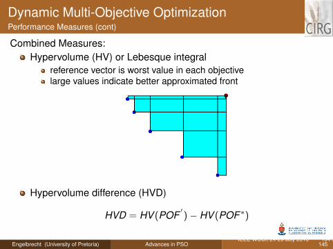
Combined Measures:Hypervolume (HV) or Lebesque integral
reference vector is worst value in each objectivelarge values indicate better approximated front
Hypervolume difference (HVD)
HVD = HV (POF′)− HV (POF ∗)
Engelbrecht (University of Pretoria) Advances in PSOIEEE WCCI, 24-29 July 2016 104 /
145
Dynamic Multi-Objective OptimizationPerformance Measures (cont)
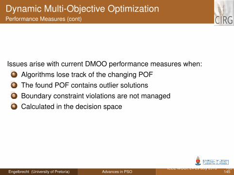
Issues arise with current DMOO performance measures when:1 Algorithms lose track of the changing POF2 The found POF contains outlier solutions3 Boundary constraint violations are not managed4 Calculated in the decision space
Engelbrecht (University of Pretoria) Advances in PSOIEEE WCCI, 24-29 July 2016 105 /
145
Dynamic Multi-Objective OptimizationPerformance Measures (cont)
DMOA loses track of changing POF, i.e. failed to track the movingPOFPOF changes over time in such a way that the HV decreases⇒ DMOAs that lose track of POF obtain the highest HVIssue of losing track of changing POF is unique to DMOOFirst observed where five algorithms solved the FDA2 DMOOP:
DVEPSO-A: uses clamping to manage boundary constraintsDVEPSO-B: uses dimension-based reinitialization to manageboundary constraintsDNSGAII-A: %individuals randomly selected and replaced with newrandomly created individualsDNSGAII-B: %individuals replaced with mutated individuals,randomly selecteddCOEA: competitive coevlutionary EA
Engelbrecht (University of Pretoria) Advances in PSOIEEE WCCI, 24-29 July 2016 106 /
145
Dynamic Multi-Objective OptimizationPerformance Measures (cont)
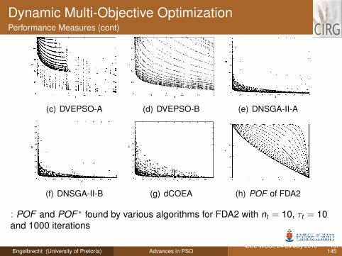
(c) DVEPSO-A (d) DVEPSO-B (e) DNSGA-II-A
(f) DNSGA-II-B (g) dCOEA (h) POF of FDA2
: POF and POF ∗ found by various algorithms for FDA2 with nt = 10, τt = 10and 1000 iterations
Engelbrecht (University of Pretoria) Advances in PSOIEEE WCCI, 24-29 July 2016 107 /
145
Dynamic Multi-Objective OptimizationPerformance Measures (cont)
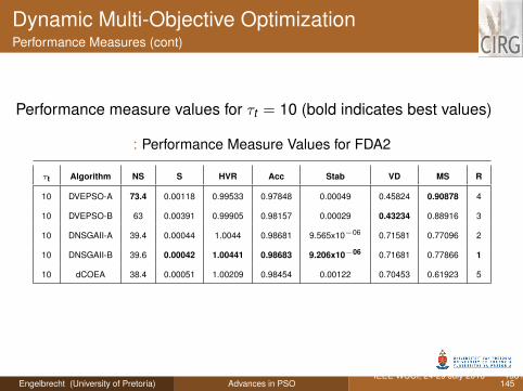
Performance measure values for τt = 10 (bold indicates best values)
: Performance Measure Values for FDA2
τt Algorithm NS S HVR Acc Stab VD MS R
10 DVEPSO-A 73.4 0.00118 0.99533 0.97848 0.00049 0.45824 0.90878 4
10 DVEPSO-B 63 0.00391 0.99905 0.98157 0.00029 0.43234 0.88916 3
10 DNSGAII-A 39.4 0.00044 1.0044 0.98681 9.565x10−06 0.71581 0.77096 2
10 DNSGAII-B 39.6 0.00042 1.00441 0.98683 9.206x10−06 0.71681 0.77866 1
10 dCOEA 38.4 0.00051 1.00209 0.98454 0.00122 0.70453 0.61923 5
Engelbrecht (University of Pretoria) Advances in PSOIEEE WCCI, 24-29 July 2016 108 /
145
Dynamic Multi-Objective OptimizationPerformance Measures (cont)
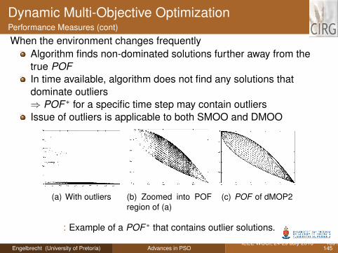
When the environment changes frequentlyAlgorithm finds non-dominated solutions further away from thetrue POFIn time available, algorithm does not find any solutions thatdominate outliers⇒ POF ∗ for a specific time step may contain outliersIssue of outliers is applicable to both SMOO and DMOO
(a) With outliers (b) Zoomed into POFregion of (a)
(c) POF of dMOP2
: Example of a POF ∗ that contains outlier solutions.
Engelbrecht (University of Pretoria) Advances in PSOIEEE WCCI, 24-29 July 2016 109 /
145
Dynamic Multi-Objective OptimizationPerformance Measures (cont)
Outliers will skew results obtained using:distance-based performance measures, such as GD, VD, PL, CS(large distances)performance measures that measure the spread of the solutions,such as MS (large diagonal), andthe HV performance measures, such as HV, HVR (outliersbecome reference vector)
Engelbrecht (University of Pretoria) Advances in PSOIEEE WCCI, 24-29 July 2016 110 /
145
Dynamic Multi-Objective OptimizationPerformance Measures (cont)
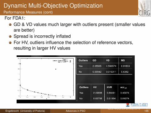
For FDA1:GD & VD values much larger with outliers present (smaller valuesare better)Spread is incorrectly inflatedFor HV, outliers influence the selection of reference vectors,resulting in larger HV values
Engelbrecht (University of Pretoria) Advances in PSOIEEE WCCI, 24-29 July 2016 111 /
145
Dynamic Multi-Objective OptimizationPerformance Measures (cont)
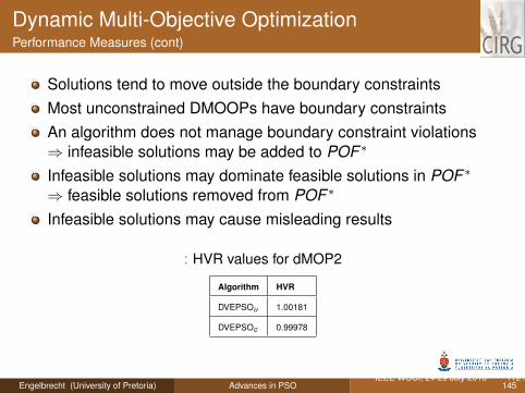
Solutions tend to move outside the boundary constraintsMost unconstrained DMOOPs have boundary constraintsAn algorithm does not manage boundary constraint violations⇒ infeasible solutions may be added to POF ∗
Infeasible solutions may dominate feasible solutions in POF ∗
⇒ feasible solutions removed from POF ∗
Infeasible solutions may cause misleading results
: HVR values for dMOP2
Algorithm HVR
DVEPSOu 1.00181
DVEPSOc 0.99978
Engelbrecht (University of Pretoria) Advances in PSOIEEE WCCI, 24-29 July 2016 112 /
145
Dynamic Multi-Objective OptimizationPerformance Measures (cont)
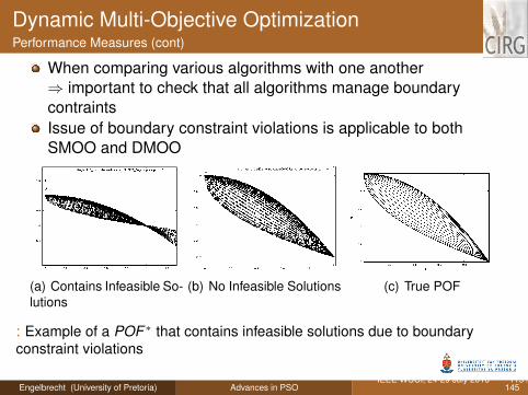
When comparing various algorithms with one another⇒ important to check that all algorithms manage boundarycontraintsIssue of boundary constraint violations is applicable to bothSMOO and DMOO
(a) Contains Infeasible So-lutions
(b) No Infeasible Solutions (c) True POF
: Example of a POF ∗ that contains infeasible solutions due to boundaryconstraint violations
Engelbrecht (University of Pretoria) Advances in PSOIEEE WCCI, 24-29 July 2016 113 /
145
Dynamic Multi-Objective OptimizationPerformance Measures (cont)
Accuracy measures (VD or GD) can be calculated in decision orobjective spaceIn objective space, VD = distance between POF ∗ and POF ′
One goal of solving a DMOOP is to track the changing POF⇒ Accuracy should be measured in objective spaceVD in decision space measures the distance between POS∗ andPOSMay be useful to determine how close POS∗ is from POSIt may occur that even though algorithm’s POS∗ is very close toPOS, POF ∗ is quite far from POFSmall change in POS may result in big change in POF, socalculation wrt decision space will be misleading
Engelbrecht (University of Pretoria) Advances in PSOIEEE WCCI, 24-29 July 2016 114 /
145
Dynamic Multi-Objective OptimizationPerformance Measures (cont)
M Helbig, AP Engelbrecht, Performance Measures for DynamicMulti-objective Optimisation Algorithms, Information Sciences,250:61–81, 2013
Engelbrecht (University of Pretoria) Advances in PSOIEEE WCCI, 24-29 July 2016 115 /
145
Dynamic Multi-Objective OptimizationVector-Evaluated Particle Swarm Optimization (VEPSO)
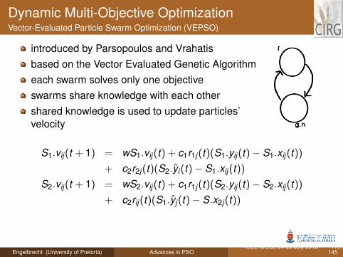
introduced by Parsopoulos and Vrahatisbased on the Vector Evaluated Genetic Algorithmeach swarm solves only one objectiveswarms share knowledge with each othershared knowledge is used to update particles’velocity
S1.vij(t + 1) = wS1.vij(t) + c1r1j(t)(S1.yij(t)− S1.xij(t))
+ c2r2j(t)(S2.yi(t)− S1.xij(t))
S2.vij(t + 1) = wS2.vij(t) + c1r1j(t)(S2.yij(t)− S2.xij(t))
+ c2rij(t)(S1.yj(t)− S.x2j(t))
Engelbrecht (University of Pretoria) Advances in PSOIEEE WCCI, 24-29 July 2016 116 /
145
Dynamic Multi-Objective OptimizationVEPSO (cont)
The VEPSO has been extended to include:an archive of non-dominated solutionsboundary contraint managementvarious ways to share knowledge among sub-swarmsupdating pbest and gbest using Pareto-dominance
Engelbrecht (University of Pretoria) Advances in PSOIEEE WCCI, 24-29 July 2016 117 /
145
Dynamic Multi-Objective OptimizationVEPSO (cont)
The archive on non-dominated solutionshas a fixed sizea new solution that is non-dominated wrt all solutions in thearchive is added to the archive if there is spacea new non-dominated solution that is dominated by any solution inthe archive is rejected, and not added to the archiveif a new solution dominates any solution in the archive, thedominated solution is removedif the archive is full, a solution from a dense area of the POF∗ isremoved
Engelbrecht (University of Pretoria) Advances in PSOIEEE WCCI, 24-29 July 2016 118 /
145
Dynamic Multi-Objective OptimizationVEPSO (cont)
If a particle violates a boundary constraint in decision space, one ofthe following strategies can be followed:
do nothing.....clamp violating dimensions at the boundary, or close to theboundarydeflection (bouncing) – invert the search directiondimension-based reinitialization to position within boundariesreinitialize entire particle
keep current velocity, orreset velocity
Engelbrecht (University of Pretoria) Advances in PSOIEEE WCCI, 24-29 July 2016 119 /
145
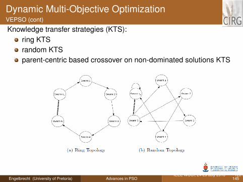
Dynamic Multi-Objective OptimizationVEPSO (cont)
Knowledge transfer strategies (KTS):ring KTSrandom KTSparent-centric based crossover on non-dominated solutions KTS
Engelbrecht (University of Pretoria) Advances in PSOIEEE WCCI, 24-29 July 2016 120 /
145
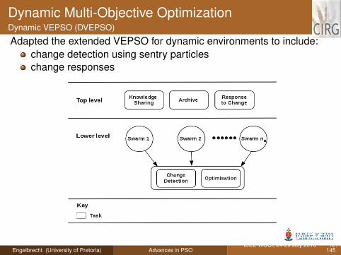
Dynamic Multi-Objective OptimizationDynamic VEPSO (DVEPSO)
Adapted the extended VEPSO for dynamic environments to include:change detection using sentry particleschange responses
Engelbrecht (University of Pretoria) Advances in PSOIEEE WCCI, 24-29 July 2016 121 /
145
Dynamic Multi-Objective OptimizationDVEPSO (cont)
Engelbrecht (University of Pretoria) Advances in PSOIEEE WCCI, 24-29 July 2016 122 /
145
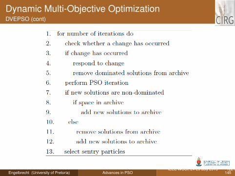
Dynamic Multi-Objective OptimizationDVEPSO (cont)
The following change detection strategy is used:Sentry particles are usedObjective function value of sentry particles evaluated at beginningand end of iterationIf there is a difference, then a change has occuredIf any one or more of the sub-swarms detect a change, then aresponse is triggered
Engelbrecht (University of Pretoria) Advances in PSOIEEE WCCI, 24-29 July 2016 123 /
145
Dynamic Multi-Objective OptimizationDVEPSO (cont)
When a change is detected, a response is activated for the affectedsub-swarm
Re-evaluationall particles and best positions re-evaluatedremove stale information
Re-initializationpercentage of particles in sub-swarm(s) re-initializedintroduces diversity
Reset pbest (local guide) to current particle positionDetermine a new gbest (global guide) position
Engelbrecht (University of Pretoria) Advances in PSOIEEE WCCI, 24-29 July 2016 124 /
145
Dynamic Multi-Objective OptimizationDVEPSO (cont)
Archive update:remove all solutions, orremove non-dominated solutions with large changes in objectivefunction values, orre-evaluate solutions
remove solutions that have become dominated, orapply hillclimbing to adapt dominated solution to becomenon-dominated
Engelbrecht (University of Pretoria) Advances in PSOIEEE WCCI, 24-29 July 2016 125 /
145
Dynamic Multi-Objective OptimizationDVEPSO (cont)
Guide updates:local guides vs global guidesupdate by not using dominanceuse dominance relation
Engelbrecht (University of Pretoria) Advances in PSOIEEE WCCI, 24-29 July 2016 126 /
145
Dynamic Multi-Objective OptimizationDVEPSO (cont)
Experimental setup:30 runs of 1000 iterations each15 benchmark functions:
change frequency, τt : 10 (1000 changes), 25 or 50change severity, nt : 1, 10, 20
Three performance measures:#non-dominated solutionsaccuracy: |HV (POF ′(t))− HV (POF ∗(t))|stability: max{acc(t − 1)− acc(t)}
Engelbrecht (University of Pretoria) Advances in PSOIEEE WCCI, 24-29 July 2016 127 /
145
Dynamic Multi-Objective OptimizationDVEPSO (cont)
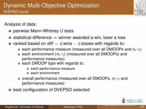
Analysis of data:pairwise Mann-Whitney U testsstatistical difference⇒ winner awarded a win, loser a lossranked based on diff = #wins −#losses with regards to:
each performance measure (measured over all DMOOPs and nt -τt )each environment (nt -τt ) (measured over all DMOOPs) andperformance measures)each DMOOP type with regards to:
each performance measureeach environment
overall performance (measured over all DMOOPs, nt -τt andperformance measures)
best configuration of DVEPSO selected
Engelbrecht (University of Pretoria) Advances in PSOIEEE WCCI, 24-29 July 2016 128 /
145
Dynamic Multi-Objective OptimizationEmpirical Analysis
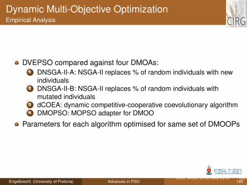
DVEPSO compared against four DMOAs:1 DNSGA-II-A: NSGA-II replaces % of random individuals with new
individuals2 DNSGA-II-B: NSGA-II replaces % of random individuals with
mutated individuals3 dCOEA: dynamic competitive-cooperative coevolutionary algorithm4 DMOPSO: MOPSO adapter for DMOO
Parameters for each algorithm optimised for same set of DMOOPs
Engelbrecht (University of Pretoria) Advances in PSOIEEE WCCI, 24-29 July 2016 129 /
145
Dynamic Multi-Objective OptimizationEmpirical Analysis (cont)
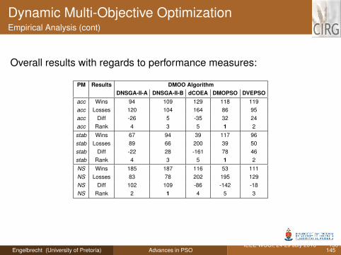
Overall results with regards to performance measures:
PM Results DMOO AlgorithmDNSGA-II-A DNSGA-II-B dCOEA DMOPSO DVEPSO
acc Wins 94 109 129 118 119acc Losses 120 104 164 86 95acc Diff -26 5 -35 32 24acc Rank 4 3 5 1 2stab Wins 67 94 39 117 96stab Losses 89 66 200 39 50stab Diff -22 28 -161 78 46stab Rank 4 3 5 1 2NS Wins 185 187 116 53 111NS Losses 83 78 202 195 129NS Diff 102 109 -86 -142 -18NS Rank 2 1 4 5 3
Engelbrecht (University of Pretoria) Advances in PSOIEEE WCCI, 24-29 July 2016 130 /
145
Dynamic Multi-Objective OptimizationEmpirical Analysis (cont)
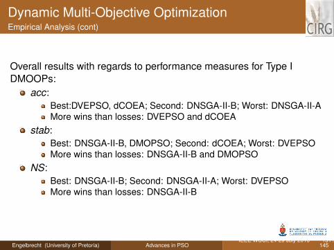
Overall results with regards to performance measures for Type IDMOOPs:
acc:Best:DVEPSO, dCOEA; Second: DNSGA-II-B; Worst: DNSGA-II-AMore wins than losses: DVEPSO and dCOEA
stab:Best: DNSGA-II-B, DMOPSO; Second: dCOEA; Worst: DVEPSOMore wins than losses: DNSGA-II-B and DMOPSO
NS:Best: DNSGA-II-B; Second: DNSGA-II-A; Worst: DVEPSOMore wins than losses: DNSGA-II-B
Engelbrecht (University of Pretoria) Advances in PSOIEEE WCCI, 24-29 July 2016 131 /
145
Dynamic Multi-Objective OptimizationEmpirical Analysis (cont)
Overall results for Type I DMOOPs:Best: DNSGA-II-B; Second: dCOEA; Worst: DNSGA-II-AMore wins than losses: DNSGA-II-A
DVEPSO:struggled to converge to POF of dMOP3 (density of non-dominatedsolutions changes over time)only algorithm converging to POF of DIMP2 (each decision variablehave a different rate of change)
Engelbrecht (University of Pretoria) Advances in PSOIEEE WCCI, 24-29 July 2016 132 /
145

Dynamic Multi-Objective OptimizationEmpirical Analysis (cont)
Results with regards to performance measures for Type II DMOOPs:
nt τt PM Results DMOO AlgorithmDNSGA-II-A DNSGA-II-B dCOEA DMOPSO DVEPSO
all all acc Wins 55 55 36 56 63all all acc Losses 43 41 106 41 34all all acc Diff 12 14 -70 15 29all all acc Rank 4 3 5 2 1all all stab Wins 36 45 18 53 59all all stab Losses 43 30 104 20 14all all stab Diff -7 15 -86 33 45all all stab Rank 4 3 5 2 1all all NS Wins 47 49 118 108 47all all NS Losses 95 91 62 34 87all all NS Diff -48 -42 56 74 -40all all NS Rank 5 4 2 1 3
Engelbrecht (University of Pretoria) Advances in PSOIEEE WCCI, 24-29 July 2016 133 /
145
Dynamic Multi-Objective OptimizationEmpirical Analysis (cont)
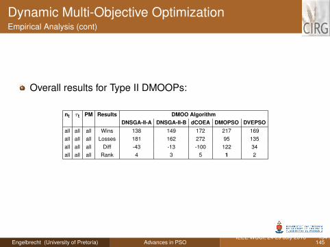
Overall results for Type II DMOOPs:
nt τt PM Results DMOO AlgorithmDNSGA-II-A DNSGA-II-B dCOEA DMOPSO DVEPSO
all all all Wins 138 149 172 217 169all all all Losses 181 162 272 95 135all all all Diff -43 -13 -100 122 34all all all Rank 4 3 5 1 2
Engelbrecht (University of Pretoria) Advances in PSOIEEE WCCI, 24-29 July 2016 134 /
145
Dynamic Multi-Objective OptimizationEmpirical Analysis (cont)
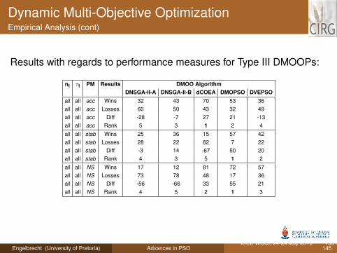
Results with regards to performance measures for Type III DMOOPs:
nt τt PM Results DMOO AlgorithmDNSGA-II-A DNSGA-II-B dCOEA DMOPSO DVEPSO
all all acc Wins 32 43 70 53 36all all acc Losses 60 50 43 32 49all all acc Diff -28 -7 27 21 -13all all acc Rank 5 3 1 2 4all all stab Wins 25 36 15 57 42all all stab Losses 28 22 82 7 22all all stab Diff -3 14 -67 50 20all all stab Rank 4 3 5 1 2all all NS Wins 17 12 81 72 57all all NS Losses 73 78 48 17 36all all NS Diff -56 -66 33 55 21all all NS Rank 4 5 2 1 3
Engelbrecht (University of Pretoria) Advances in PSOIEEE WCCI, 24-29 July 2016 135 /
145
Dynamic Multi-Objective OptimizationEmpirical Analysis (cont)
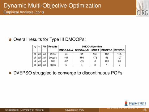
Overall results for Type III DMOOPs:nt τt PM Results DMOO Algorithm
DNSGA-II-A DNSGA-II-B dCOEA DMOPSO DVEPSOall all all Wins 74 91 166 182 135all all all Losses 161 150 173 56 107all all all Diff -87 -59 -7 126 28all all all Rank 5 4 3 1 2
DVEPSO struggled to converge to discontinuous POFs
Engelbrecht (University of Pretoria) Advances in PSOIEEE WCCI, 24-29 July 2016 136 /
145
Dynamic Multi-Objective OptimizationEmpirical Analysis (cont)
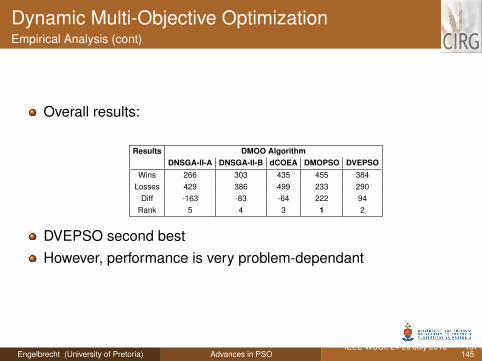
Overall results:
Results DMOO AlgorithmDNSGA-II-A DNSGA-II-B dCOEA DMOPSO DVEPSO
Wins 266 303 435 455 384Losses 429 386 499 233 290
Diff -163 -83 -64 222 94Rank 5 4 3 1 2
DVEPSO second bestHowever, performance is very problem-dependant
Engelbrecht (University of Pretoria) Advances in PSOIEEE WCCI, 24-29 July 2016 137 /
145
Dynamic Multi-Objective OptimizationEmpirical Analysis (cont)
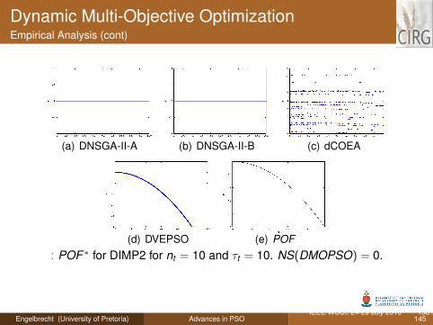
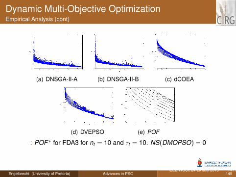
(a) DNSGA-II-A (b) DNSGA-II-B (c) dCOEA
(d) DVEPSO (e) POF: POF ∗ for DIMP2 for nt = 10 and τt = 10. NS(DMOPSO) = 0.
Engelbrecht (University of Pretoria) Advances in PSOIEEE WCCI, 24-29 July 2016 138 /
145
Dynamic Multi-Objective OptimizationEmpirical Analysis (cont)
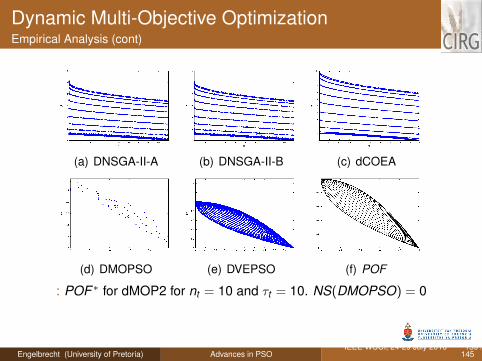
(a) DNSGA-II-A (b) DNSGA-II-B (c) dCOEA
(d) DMOPSO (e) DVEPSO (f) POF
: POF ∗ for dMOP2 for nt = 10 and τt = 10. NS(DMOPSO) = 0
Engelbrecht (University of Pretoria) Advances in PSOIEEE WCCI, 24-29 July 2016 139 /
145
Dynamic Multi-Objective OptimizationEmpirical Analysis (cont)
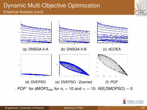
(a) DNSGA-II-A (b) DNSGA-II-B (c) dCOEA
(d) DVEPSO (e) DVEPSO - Zoomed (f) POF
: POF ∗ for dMOP2dec for nt = 10 and τt = 10. NS(DMOPSO) = 0
Engelbrecht (University of Pretoria) Advances in PSOIEEE WCCI, 24-29 July 2016 140 /
145
Dynamic Multi-Objective OptimizationEmpirical Analysis (cont)
(a) DNSGA-II-A (b) DNSGA-II-B (c) dCOEA
(d) DVEPSO (e) POF
: POF ∗ for FDA3 for nt = 10 and τt = 10. NS(DMOPSO) = 0
Engelbrecht (University of Pretoria) Advances in PSOIEEE WCCI, 24-29 July 2016 141 /
145
Dynamic Multi-Objective OptimizationEmpirical Analysis (cont)
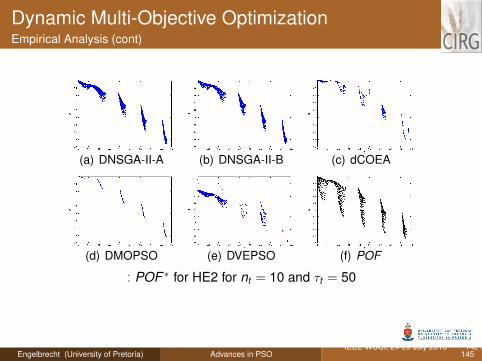
(a) DNSGA-II-A (b) DNSGA-II-B (c) dCOEA
(d) DMOPSO (e) DVEPSO (f) POF
: POF ∗ for HE2 for nt = 10 and τt = 50
Engelbrecht (University of Pretoria) Advances in PSOIEEE WCCI, 24-29 July 2016 142 /
145
Heterogeneous Dynamic Vector-Evaluated ParticleSwarm OptimizationHDEVEPSO
The heterogeneous DVEPSOEach sub-swarm is an HPSOBehavior selected when change in sub-swarm detected, orpbest stagnated for a number of iterations
Engelbrecht (University of Pretoria) Advances in PSOIEEE WCCI, 24-29 July 2016 143 /
145
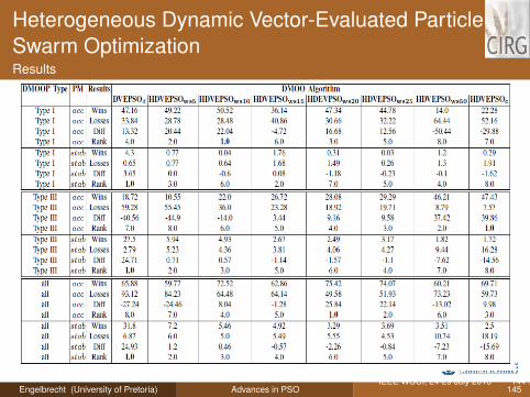
Heterogeneous Dynamic Vector-Evaluated ParticleSwarm OptimizationResults
Engelbrecht (University of Pretoria) Advances in PSOIEEE WCCI, 24-29 July 2016 144 /
145
Summary
Research in PSO has been very active over the past two decades, andthere are still much scope for more research, to focus on:
Further theoretical analyses of PSOPSO for dynamic multi-objective optimization problemsPSO for static and dynamic many-objective optimization problemsPSO for dynamically changing constraintsSet-based PSO algorithmsApplication of PSO to new real-world problems not yet solved
Engelbrecht (University of Pretoria) Advances in PSOIEEE WCCI, 24-29 July 2016 145 /
145