Embed Size (px)
Citation preview

Advanced Monte Carlo Methods:American Options
Prof. Mike Giles
Oxford University Mathematical Institute
American options – p. 1
Early Exercise
Perhaps the biggest challenge for Monte Carlo methods isthe accurate and efficient pricing of options with optionalearly exercise:
Bermudan options: can exercise at a finite number oftimes tjAmerican options: can exercise at any time
The challenge is to find/approximate the optimal strategy(i.e. when to exercise) and hence determine the price andGreeks.
American options – p. 2
Early Exercise
Approximating the optimal exercise boundary introducesnew approximation errors:
An approximate exercise boundary is inevitablysub-optimal=⇒ under-estimate of “true” value, but accurate valuefor the sub-optimal strategy
For the option buyer, sub-optimal price reflects valueachievable with sub-optimal strategy
For the option seller, “true” price is best a purchasermight achieve
Can also derive an upper bound approximation
American options – p. 3
Early Exercise
Why is early exercise so difficult for Monte Carlo methods?
leads naturally to a dynamic programming formulationworking backwards in time
fairly minor extension for finite difference methodswhich already march backwards in time
doesn’t fit well with Monte Carlo methods which goforwards in time
American options – p. 4
Problem Formulation
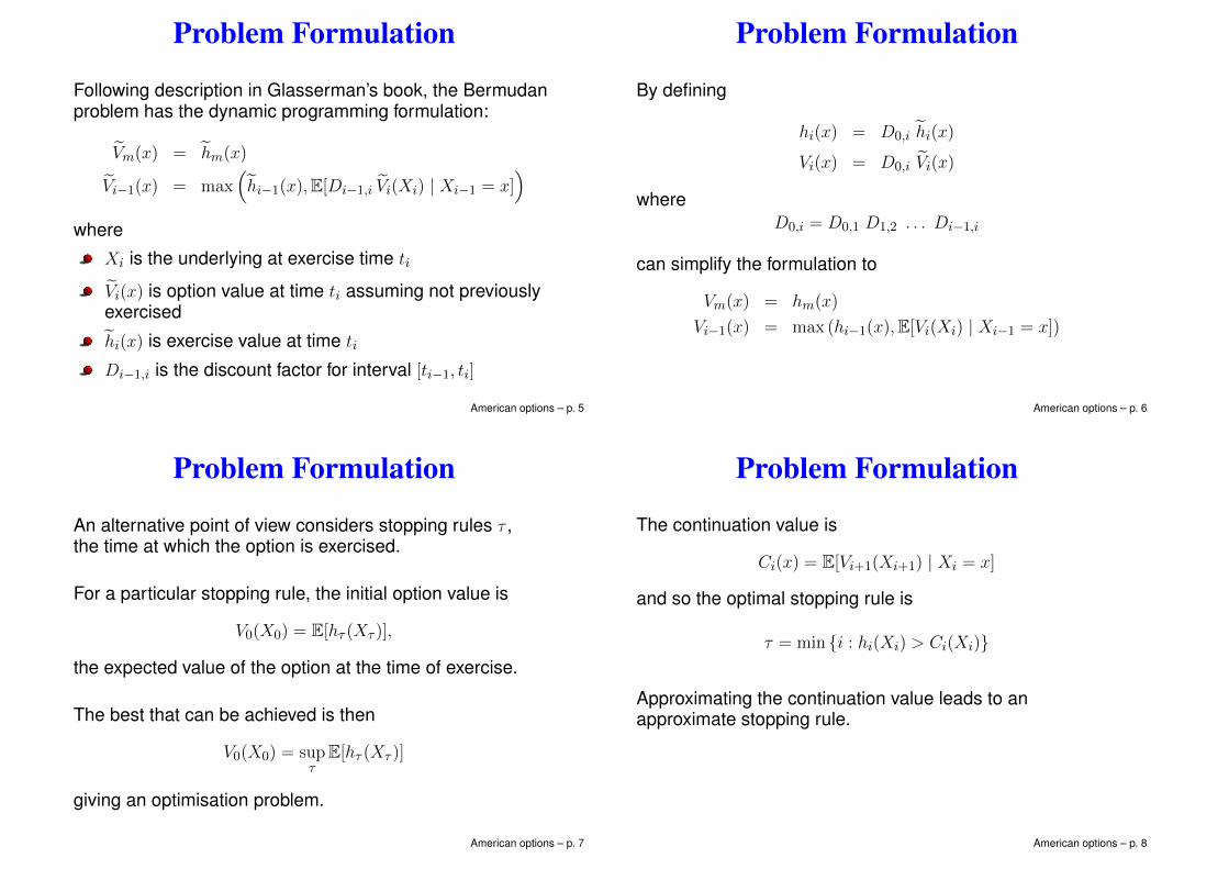
Following description in Glasserman’s book, the Bermudanproblem has the dynamic programming formulation:
Vm(x) = hm(x)
Vi−1(x) = max(hi−1(x),E[Di−1,i Vi(Xi) | Xi−1 = x]
)
where
Xi is the underlying at exercise time ti
Vi(x) is option value at time ti assuming not previouslyexercised
hi(x) is exercise value at time tiDi−1,i is the discount factor for interval [ti−1, ti]
American options – p. 5
Problem Formulation
By defining
hi(x) = D0,i hi(x)
Vi(x) = D0,i Vi(x)
whereD0,i = D0,1 D1,2 . . . Di−1,i
can simplify the formulation to
Vm(x) = hm(x)
Vi−1(x) = max (hi−1(x),E[Vi(Xi) | Xi−1 = x])
American options – p. 6
Problem Formulation
An alternative point of view considers stopping rules τ ,the time at which the option is exercised.
For a particular stopping rule, the initial option value is
V0(X0) = E[hτ (Xτ )],
the expected value of the option at the time of exercise.
The best that can be achieved is then
V0(X0) = supτ
E[hτ (Xτ )]
giving an optimisation problem.
American options – p. 7
Problem Formulation
The continuation value is
Ci(x) = E[Vi+1(Xi+1) | Xi = x]
and so the optimal stopping rule is
τ = min i : hi(Xi) > Ci(Xi)
Approximating the continuation value leads to anapproximate stopping rule.
American options – p. 8
Longstaff-Schwartz Method
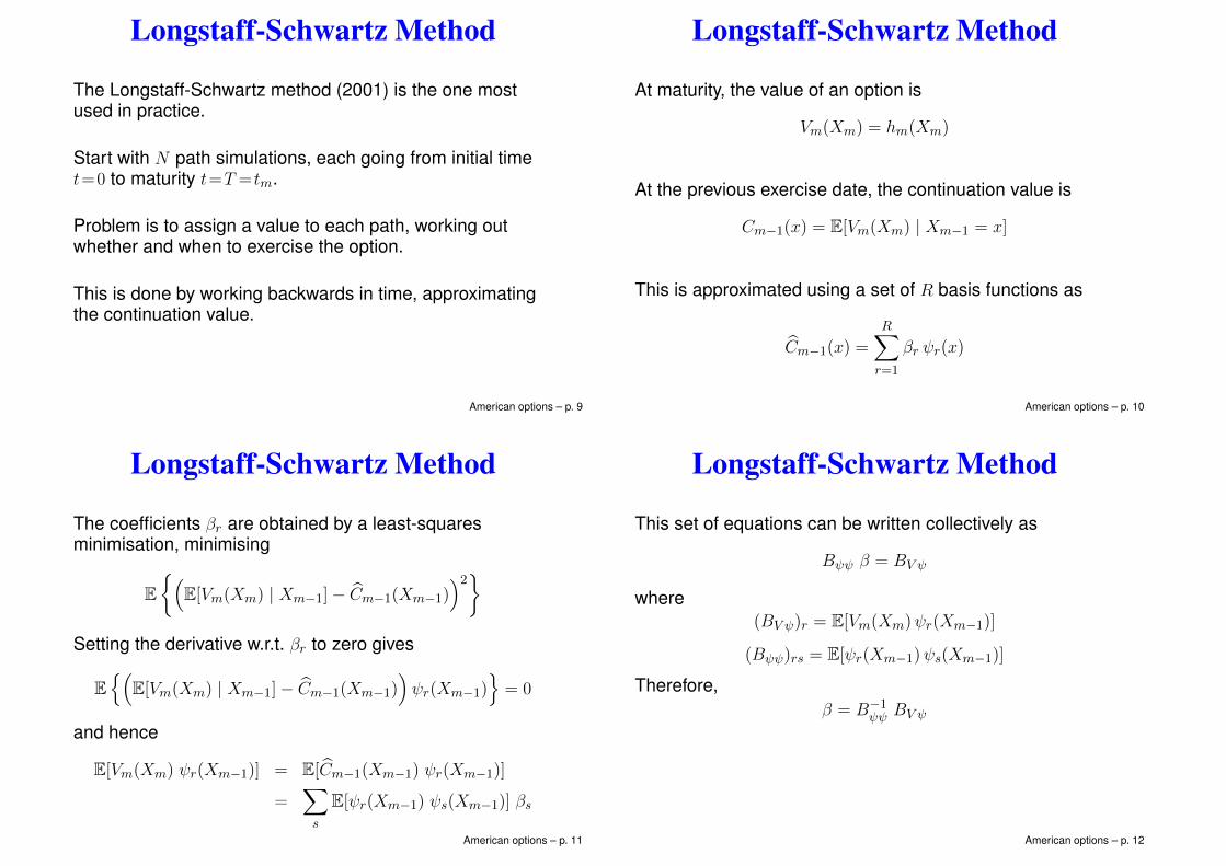
The Longstaff-Schwartz method (2001) is the one mostused in practice.
Start with N path simulations, each going from initial timet=0 to maturity t=T = tm.
Problem is to assign a value to each path, working outwhether and when to exercise the option.
This is done by working backwards in time, approximatingthe continuation value.
American options – p. 9
Longstaff-Schwartz Method
At maturity, the value of an option is
Vm(Xm) = hm(Xm)
At the previous exercise date, the continuation value is
Cm−1(x) = E[Vm(Xm) | Xm−1 = x]
This is approximated using a set of R basis functions as
Cm−1(x) =
R∑
r=1
βr ψr(x)
American options – p. 10
Longstaff-Schwartz Method
The coefficients βr are obtained by a least-squaresminimisation, minimising
E(
E[Vm(Xm) | Xm−1]− Cm−1(Xm−1))2
Setting the derivative w.r.t. βr to zero gives
E(
E[Vm(Xm) | Xm−1]− Cm−1(Xm−1))ψr(Xm−1)
= 0
and hence
E[Vm(Xm) ψr(Xm−1)] = E[Cm−1(Xm−1) ψr(Xm−1)]
=∑
s
E[ψr(Xm−1) ψs(Xm−1)] βs
American options – p. 11
Longstaff-Schwartz Method
This set of equations can be written collectively as
Bψψ β = BV ψ
where(BV ψ)r = E[Vm(Xm)ψr(Xm−1)]
(Bψψ)rs = E[ψr(Xm−1)ψs(Xm−1)]
Therefore,β = B−1
ψψ BV ψ
American options – p. 12
Longstaff-Schwartz Method
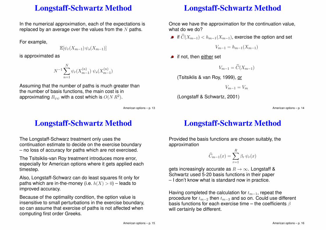
In the numerical approximation, each of the expectations isreplaced by an average over the values from the N paths.
For example,E[ψr(Xm−1)ψs(Xm−1)]
is approximated as
N−1N∑
n=1
ψr(X(n)m−1) ψs(X
(n)m−1)
Assuming that the number of paths is much greater thanthe number of basis functions, the main cost is inapproximating Bψψ with a cost which is O(N R2).
American options – p. 13
Longstaff-Schwartz Method
Once we have the approximation for the continuation value,what do we do?
if C(Xm−1) < hm−1(Xm−1), exercise the option and set
Vm−1 = hm−1(Xm−1)
if not, then either set
Vm−1 = C(Xm−1)
(Tsitsiklis & van Roy, 1999), or
Vm−1 = Vm
(Longstaff & Schwartz, 2001)
American options – p. 14
Longstaff-Schwartz Method
The Longstaff-Schwarz treatment only uses thecontinuation estimate to decide on the exercise boundary– no loss of accuracy for paths which are not exercised.
The Tsitsiklis-van Roy treatment introduces more error,especially for American options where it gets applied eachtimestep.
Also, Longstaff-Schwarz can do least squares fit only forpaths which are in-the-money (i.e. h(X) > 0) – leads toimproved accuracy.
Because of the optimality condition, the option value isinsensitive to small perturbations in the exercise boundary,so can assume that exercise of paths is not affected whencomputing first order Greeks.
American options – p. 15
Longstaff-Schwartz Method
Provided the basis functions are chosen suitably, theapproximation
Cm−1(x) =
R∑
r=1
βr ψr(x)
gets increasingly accurate as R → ∞. Longstaff &Schwartz used 5-20 basis functions in their paper– I don’t know what is standard now in practice.
Having completed the calculation for tm−1, repeat theprocedure for tm−2 then tm−3 and so on. Could use differentbasis functions for each exercise time – the coefficients βwill certainly be different.
American options – p. 16
Longstaff-Schwartz Method
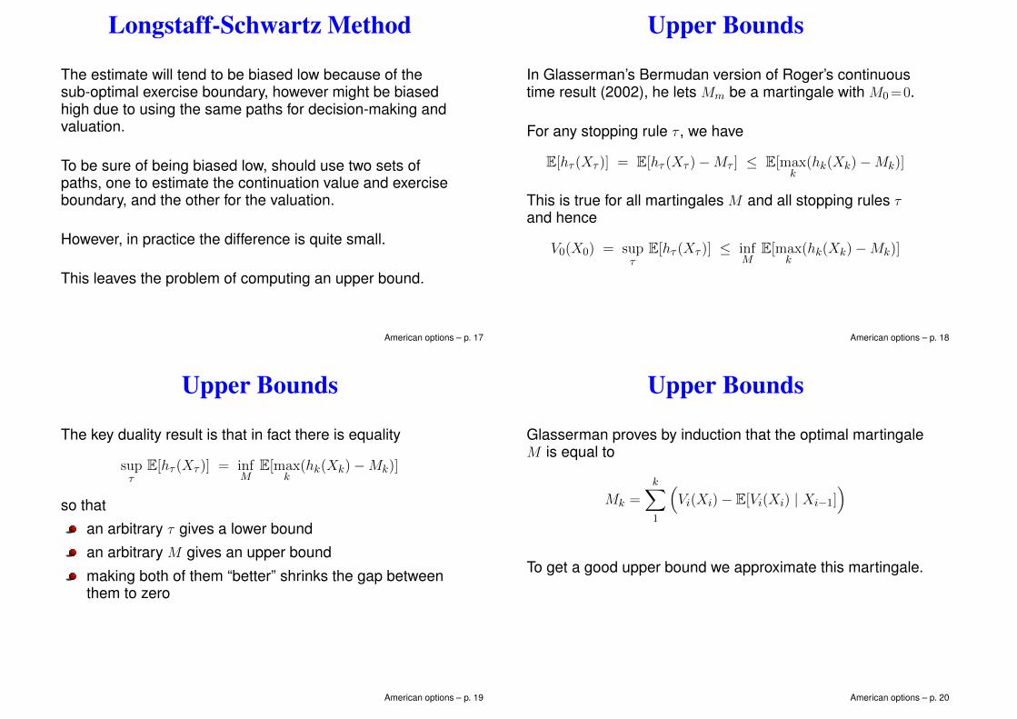
The estimate will tend to be biased low because of thesub-optimal exercise boundary, however might be biasedhigh due to using the same paths for decision-making andvaluation.
To be sure of being biased low, should use two sets ofpaths, one to estimate the continuation value and exerciseboundary, and the other for the valuation.
However, in practice the difference is quite small.
This leaves the problem of computing an upper bound.
American options – p. 17
Upper Bounds
In Glasserman’s Bermudan version of Roger’s continuoustime result (2002), he lets Mm be a martingale with M0=0.
For any stopping rule τ , we have
E[hτ (Xτ )] = E[hτ (Xτ )−Mτ ] ≤ E[maxk
(hk(Xk)−Mk)]
This is true for all martingales M and all stopping rules τand hence
V0(X0) = supτ
E[hτ (Xτ )] ≤ infM
E[maxk
(hk(Xk)−Mk)]
American options – p. 18
Upper Bounds
The key duality result is that in fact there is equality
supτ
E[hτ (Xτ )] = infM
E[maxk
(hk(Xk)−Mk)]
so that
an arbitrary τ gives a lower bound
an arbitrary M gives an upper bound
making both of them “better” shrinks the gap betweenthem to zero
American options – p. 19
Upper Bounds
Glasserman proves by induction that the optimal martingaleM is equal to
Mk =
k∑
1
(Vi(Xi)− E[Vi(Xi) | Xi−1]
)
To get a good upper bound we approximate this martingale.
American options – p. 20
Upper Bounds
The approximate martingale for a particular path is definedas
Mk =
k∑
1
(Vi(Xi)− P−1
∑
p
Vi(X(p)i )
)
where the X(p)i are values for Xi from P different mini-paths
starting at Xi−1, and
Vi(Xi) = max(hi(Xi), Ci(Xi))
with Ci(Xi) being the approximate continuation value givenby the Longstaff-Schwartz algorithm.
Glasserman suggests up to 100 mini-paths may be needed.American options – p. 21
Final Words
Bermudan and American options are importantapplications
Longstaff-Schwartz method is popular, but still plentyof scope for improvement?
suspect that finite difference method is used forGreeks?
is independent second set of paths used in practice?
are upper bounds used in practice?
American options – p. 22

Advanced Monte Carlo Methods:Quasi-Monte Carlo
Prof. Mike Giles
Oxford University Mathematical Institute
QMC – p. 1
Quasi Monte Carlo
low discrepancy sequences
Koksma-Hlawka inequality
rank-1 lattice rules and Sobol sequences
randomised QMC
identification of dominant dimension
QMC – p. 2
Quasi Monte Carlo
Standard Monte Carlo approximates high-dimensionalhypercube integral ∫
[0,1]df(x) dx
by
1
N
N∑
i=1
f(x(i))
with points chosen randomly, giving
r.m.s. error proportional to N−1/2
confidence interval
QMC – p. 3
Quasi Monte Carlo
Standard quasi Monte Carlo uses the same equal-weightestimator
1
N
N∑
i=1
f(x(i))
but chooses the points systematically so that
error roughly proportional to N−1
no confidence interval
(We’ll get the confidence interval back later by adding insome randomisation!)
QMC – p. 4
Low Discrepancy Sequences
The key is to use points which are fairly uniformly spreadwithin the hypercube, not clustered anywhere.
The star discrepancy D∗N (x(1), . . . x(N)) of a set of N points
is defined as
D∗N = sup
B∈J
∣∣∣∣A(B)
N− λ(B)
∣∣∣∣
where J is the set of all hyper-rectangles of the form∏
[u−i , u+i ], u±i ∈ [0, 1],
A(B) is the number of points in B, and λ(B) is the volume(or measure) of B.
QMC – p. 5
Low Discrepancy Sequences
There are sequences for which
D∗N ≤ C
(logN)d
N
where d is the dimension of the problem.
This is important because of the Koksma-Hlawka inequality.
QMC – p. 6
Koksma-Hlawka Inequality∣∣∣∣∣1
N
N∑
i=1
f(x(i))−∫
[0,1]df(x) dx
∣∣∣∣∣ ≤ V (f) D∗N (x(1), . . . x(N))
where V (f) is the Hardy-Krause variation of f defined (forsufficiently differentiable f ) as a sum of terms of the form
∫
[0,1]k
∣∣∣∣∂kf
∂xi1 . . . ∂xik
∣∣∣∣xj=1,j 6=i1,...,ik
dx
with i1<i2<. . .<ik for k ≤ d.
Problem: not a useful error bound
in finance applications f often isn’t even bounded
even when it is, it’s not sufficiently differentiable andestimating V (f) is computationally demanding QMC – p. 7
Koksma-Hlawka Inequality
However, still useful because of what it tells us about theasymptotic behaviour:
Error < C(logN)d
N
for small dimension d, (d<10?) this is much better thanN−1/2 r.m.s. error for standard MC
for large dimension d, (logN)d could be enormous,so not clear there is any benefit
QMC – p. 8
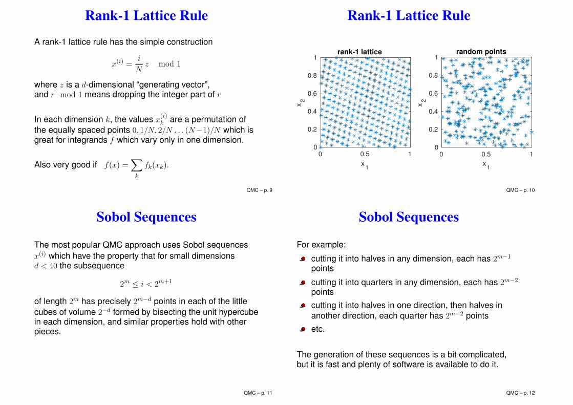
Rank-1 Lattice Rule
A rank-1 lattice rule has the simple construction
x(i) =i
Nz mod 1
where z is a d-dimensional “generating vector”,and r mod 1 means dropping the integer part of r
In each dimension k, the values x(i)k are a permutation of
the equally spaced points 0, 1/N, 2/N . . . (N−1)/N which isgreat for integrands f which vary only in one dimension.
Also very good if f(x) =∑
k
fk(xk).
QMC – p. 9
Rank-1 Lattice Rule
Two dimensions: 256 points
0 0.5 1
x1
0
0.2
0.4
0.6
0.8
1
x2
rank-1 lattice
0 0.5 1
x1
0
0.2
0.4
0.6
0.8
1
x2
random points
QMC – p. 10
Sobol Sequences
The most popular QMC approach uses Sobol sequencesx(i) which have the property that for small dimensionsd < 40 the subsequence
2m ≤ i < 2m+1
of length 2m has precisely 2m−d points in each of the littlecubes of volume 2−d formed by bisecting the unit hypercubein each dimension, and similar properties hold with otherpieces.
QMC – p. 11
Sobol Sequences
For example:
cutting it into halves in any dimension, each has 2m−1
points
cutting it into quarters in any dimension, each has 2m−2
points
cutting it into halves in one direction, then halves inanother direction, each quarter has 2m−2 points
etc.
The generation of these sequences is a bit complicated,but it is fast and plenty of software is available to do it.
QMC – p. 12
Sobol sequences
Two dimensions: 256 points
0 0.5 1
x1
0
0.2
0.4
0.6
0.8
1
x2
Sobol points
0 0.5 1
x1
0
0.2
0.4
0.6
0.8
1
x2
random points
QMC – p. 13
Randomised QMC
In the best cases, QMC error is O(N−1) instead of O(N−1/2)but without a confidence interval.
To get a confidence interval using a rank-1 lattice rule,we use several sets of QMC points, with the N pointsin set m defined by
x(i,m) =
(i
Nz + x(m)
)mod 1
where x(m) is a random offset vector.
QMC – p. 14
Randomised QMC
For each m, let
fm =1
N
N∑
i=1
f(x(i,m))
This is a random variable, and since E[f(x(i,m))] = E[f ]it follows that E[fm] = E[f ]
By using multiple sets, we can estimate V[f ] in the usualway and so get a confidence interval
More sets =⇒ better variance estimate, but poorer error.Some people use as few as 10 sets, but I prefer 32.
QMC – p. 15
Randomised QMC
For Sobol sequences, randomisation is achieved throughdigital scrambling:
x(i,m) = x(i)∨ X(m)
where the exclusive-or operation ∨ is applied bitwise so that
0.1010011
∨ 0.0110110
= 0.1100101
The benefit of the digital scrambling is that it maintains thespecial properties of the Sobol sequence.
QMC – p. 16
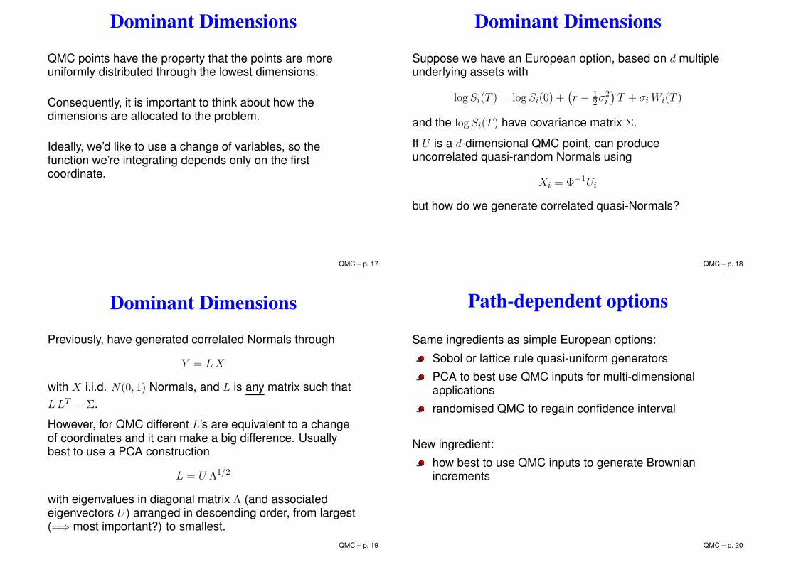
Dominant Dimensions
QMC points have the property that the points are moreuniformly distributed through the lowest dimensions.
Consequently, it is important to think about how thedimensions are allocated to the problem.
Ideally, we’d like to use a change of variables, so thefunction we’re integrating depends only on the firstcoordinate.
QMC – p. 17
Dominant Dimensions
Suppose we have an European option, based on d multipleunderlying assets with
log Si(T ) = log Si(0) +(r − 1
2σ2i
)T + σiWi(T )
and the log Si(T ) have covariance matrix Σ.
If U is a d-dimensional QMC point, can produceuncorrelated quasi-random Normals using
Xi = Φ−1Ui
but how do we generate correlated quasi-Normals?
QMC – p. 18
Dominant Dimensions
Previously, have generated correlated Normals through
Y = LX
with X i.i.d. N(0, 1) Normals, and L is any matrix such thatLLT = Σ.
However, for QMC different L’s are equivalent to a changeof coordinates and it can make a big difference. Usuallybest to use a PCA construction
L = U Λ1/2
with eigenvalues in diagonal matrix Λ (and associatedeigenvectors U ) arranged in descending order, from largest(=⇒ most important?) to smallest.
QMC – p. 19
Path-dependent options
Same ingredients as simple European options:
Sobol or lattice rule quasi-uniform generators
PCA to best use QMC inputs for multi-dimensionalapplications
randomised QMC to regain confidence interval
New ingredient:
how best to use QMC inputs to generate Brownianincrements
QMC – p. 20

Quasi-Monte Carlo
When using standard Normal random inputs for MCsimulation, can express expectation as a multi-dimensionalintegral with respect to inputs
V = E[f(S)] =∫
f(S) φ(Z) dZ
where φ(Z) is multi-dimensional standard Normal p.d.f.
Putting Zn = Φ−1Un turns this into an integral over aM -dimensional hypercube
V = E[f(S)] =∫
f(S) dU
QMC – p. 21
Quasi-Monte Carlo
This is then approximated as
N−1∑
n
f(S(n))
and each path calculation involves the computations
U → Z → ∆W → S → f
The key step here is the second, how best to convert thevector Z into the vector ∆W . With standard Monte Carlo, aslong as ∆W has the correct distribution, how it is generatedis irrelevant, but with QMC it does matter.
QMC – p. 22
Quasi-Monte Carlo
For a scalar Brownian motion W (t) with W (0)=0, definingWn=W (nh), each Wn is Normally distributed and for j ≥ k
E[Wj Wk] = E[W 2k ] + E[(Wj−Wk)Wk] = tk
since Wj−Wk is independent of Wk.
Hence, the covariance matrix for W is Ω with elements
Ωj,k = min(tj , tk)
QMC – p. 23
Quasi-Monte Carlo
The task now is to find a matrix L such that
L LT = Ω = h
1 1 . . . 1 1
1 2 . . . 2 2
. . . . . . . . . . . . . . .
1 2 . . . M−1 M−1
1 2 . . . M−1 M
We will consider 3 possibilities:
Cholesky factorisation
PCA
Brownian Bridge treatmentQMC – p. 24
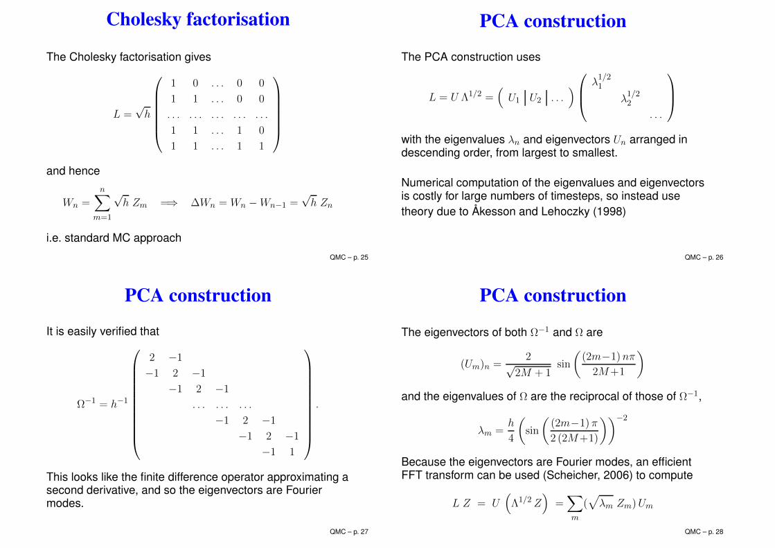
Cholesky factorisation
The Cholesky factorisation gives
L =√h
1 0 . . . 0 0
1 1 . . . 0 0
. . . . . . . . . . . . . . .
1 1 . . . 1 0
1 1 . . . 1 1
and hence
Wn =
n∑
m=1
√h Zm =⇒ ∆Wn = Wn −Wn−1 =
√h Zn
i.e. standard MC approach
QMC – p. 25
PCA construction
The PCA construction uses
L = U Λ1/2 =(
U1 U2 . . .)
λ1/21
λ1/22
. . .
with the eigenvalues λn and eigenvectors Un arranged indescending order, from largest to smallest.
Numerical computation of the eigenvalues and eigenvectorsis costly for large numbers of timesteps, so instead usetheory due to Åkesson and Lehoczky (1998)
QMC – p. 26
PCA construction
It is easily verified that
Ω−1 = h−1
2 −1
−1 2 −1
−1 2 −1
. . . . . . . . .
−1 2 −1
−1 2 −1
−1 1
.
This looks like the finite difference operator approximating asecond derivative, and so the eigenvectors are Fouriermodes.
QMC – p. 27
PCA construction
The eigenvectors of both Ω−1 and Ω are
(Um)n =2√
2M + 1sin
((2m−1)nπ
2M+1
)
and the eigenvalues of Ω are the reciprocal of those of Ω−1,
λm =h
4
(sin
((2m−1) π
2 (2M+1)
))−2
Because the eigenvectors are Fourier modes, an efficientFFT transform can be used (Scheicher, 2006) to compute
L Z = U(Λ1/2 Z
)=
∑
m
(√
λm Zm)Um
QMC – p. 28

Brownian Bridge construction
The Brownian Bridge construction uses the theory from aprevious lecture.
The final Brownian value is constructed using Z1:
WM =√T Z1
Conditional on this, the midpoint value WM/2 is Normallydistributed with mean 1
2WM and variance T/4, and so canbe constructed as
WM/2 =12WM +
√T/4 Z2
QMC – p. 29
Brownian Bridge construction
The quarter and three-quarters points can then beconstructed as
WM/4 = 12WM/2 +
√T/8 Z3
W3M/4 = 12(WM/2 +WM ) +
√T/8 Z4
and the procedure continued recursively until all Brownianvalues are defined.
(This assumes M is a power of 2 – if not, theimplementation is slightly more complex)
I have a slight preference for this method because it isparticularly effective for European option for which S(T ) isvery strongly dependent on W (T ).
QMC – p. 30
Multi-dimensional Brownian motion
The preceding discussion concerns the construction of asingle, scalar Brownian motion.
Suppose now that we have to generate a P -dimensionalBrownian motion with correlation matrix Σ between thedifferent components.
What do we do?
QMC – p. 31
Multi-dimensional Brownian motion
First, using either PCA or BB to construct P uncorrelatedBrownian paths using
Z1, Z1+P , Z1+2P , Z1+3P , . . . for first path
Z2, Z2+P , Z2+2P , Z2+3P , . . . for second path
Z3, Z3+P , Z3+2P , Z3+3P , . . . for third path
etc.
This uses the “best” dimensions of Z for the overallbehaviour of all of the paths.
QMC – p. 32
Multi-dimensional Brownian motion
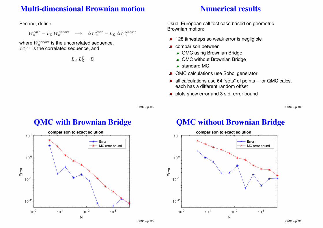
Second, define
W corrn = LΣ W uncorr
n =⇒ ∆W corrn = LΣ ∆W uncorr
n
where W uncorrn is the uncorrelated sequence,
W corrn is the correlated sequence, and
LΣ LTΣ = Σ
QMC – p. 33
Numerical results
Usual European call test case based on geometricBrownian motion:
128 timesteps so weak error is negligible
comparison betweenQMC using Brownian BridgeQMC without Brownian Bridgestandard MC
QMC calculations use Sobol generator
all calculations use 64 “sets” of points – for QMC calcs,each has a different random offset
plots show error and 3 s.d. error bound
QMC – p. 34
QMC with Brownian Bridge
100
101
102
103
N
10-2
10-1
100
101
Err
or
comparison to exact solution
Error
MC error bound
QMC – p. 35
QMC without Brownian Bridge
100
101
102
103
N
10-2
10-1
100
101
Err
or
comparison to exact solution
Error
MC error bound
QMC – p. 36
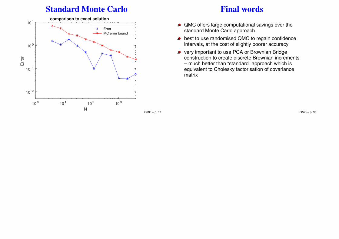
Standard Monte Carlo
100
101
102
103
N
10-2
10-1
100
101
Err
or
comparison to exact solution
Error
MC error bound
QMC – p. 37
Final words
QMC offers large computational savings over thestandard Monte Carlo approach
best to use randomised QMC to regain confidenceintervals, at the cost of slightly poorer accuracy
very important to use PCA or Brownian Bridgeconstruction to create discrete Brownian increments– much better than “standard” approach which isequivalent to Cholesky factorisation of covariancematrix
QMC – p. 38
Advanced Monte Carlo Methods:Computing Greeks
Prof. Mike Giles
Oxford University Mathematical Institute
Computing Greeks – p. 1
Outline
Computing Greeks
finite differences
likelihood ratio method
pathwise sensitivities
“Smoking adjoints” implementation
Computing Greeks – p. 2
SDE path simulation
For the generic stochastic differential equation
dS(t) = a(S) dt+ b(S) dW (t)
an Euler approximation with timestep h is
Sn+1 = Sn + a(Sn)h+ b(Sn)Zn
√h,
where Z is a N(0, 1) random variable. To estimate the valueof a European option
V = E[f(S(T ))],we take the average of N paths with M timesteps:
V = N−1∑
i
f(S(i)M ).
Computing Greeks – p. 3
Greeks
As in Module 2, in addition to estimating the expected value
V = E[f(S(T )],
we also want to know a whole range of “Greeks”corresponding to first and second derivatives of V withrespect to various parameters:
∆ =∂V
∂S0, Γ =
∂2V
∂S20
,
ρ =∂V
∂r, Vega =
∂V
∂σ.
These are needed for hedging and for risk analysis.
Computing Greeks – p. 4
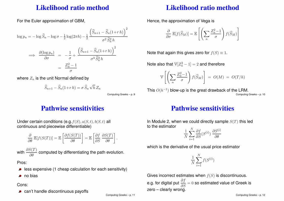
Finite difference sensitivities
If V (θ) = E[f(S(T ))] for a particular value of an input
parameter θ, then the sensitivity∂V
∂θcan be approximated
by one-sided finite difference
∂V
∂θ=
V (θ+∆θ)− V (θ)
∆θ+ O(∆θ)
or by central finite difference
∂V
∂θ=
V (θ+∆θ)− V (θ−∆θ)
2∆θ+ O((∆θ)2)
Nothing changes here from Module 2 because of the pathsimulation.
Computing Greeks – p. 5
Finite difference sensitivities
As before, the clear advantage of this approach is that it isvery simple to implement (hence the most popular inpractice?)
However, the disadvantages are:
expensive (2 extra sets of calculations for centraldifferences)
significant bias error if ∆θ too large
large variance if f(S(T )) discontinuous and ∆θ small
Also, very important to use the same random numbers forthe “bumped” path simulations to minimise the variance.
Computing Greeks – p. 6
Likelihood ratio method
As a recap from Module 2, if we define p(S) to theprobability density function for the final state S(T ), then
V = E[f(S(T ))] =∫
f(S) p(S) dS,
=⇒ ∂V
∂θ=
∫f∂p
∂θdS =
∫f∂(log p)
∂θp dS = E
[f∂(log p)
∂θ
]
The quantity∂(log p)
∂θis sometimes called the “score
function”.
Computing Greeks – p. 7
Likelihood ratio method
Extending LRM to a SDE path simulation with M timesteps,with the payoff a function purely of the discrete states Sn,we have the M -dimensional integral
V = E[f(S)] =∫
f(S) p(S) dS,
where dS ≡ dS1 dS2 dS3 . . . dSM
and p(S) is the product of the p.d.f.s for each timestep
p(S) =∏
n
pn(Sn+1|Sn)
log p(S) =∑
n
log pn(Sn+1|Sn)
Computing Greeks – p. 8
Likelihood ratio method
For the Euler approximation of GBM,
log pn = − log Sn− log σ− 12 log(2πh)− 1
2
(Sn+1 − Sn(1+r h)
)2
σ2 S2n h
=⇒ ∂(log pn)
∂σ= − 1
σ+
(Sn+1 − Sn(1+r h)
)2
σ3 S2n h
=Z2n − 1
σ
where Zn is the unit Normal defined by
Sn+1 − Sn(1+r h) = σ Sn
√hZn
Computing Greeks – p. 9
Likelihood ratio method
Hence, the approximation of Vega is
∂
∂σE[f(SM )] = E
[(∑
n
Z2n−1
σ
)f(SM )
]
Note that again this gives zero for f(S) ≡ 1.
Note also that V[Z2n − 1] = 2 and therefore
V
[(∑
n
Z2n−1
σ
)f(SM )
]= O(M) = O(T/h)
This O(h−1) blow-up is the great drawback of the LRM.Computing Greeks – p. 10
Pathwise sensitivities
Under certain conditions (e.g.f(S), a(S, t), b(S, t) allcontinuous and piecewise differentiable)
∂
∂θE[f(S(T ))] = E
[∂f(S(T ))
∂θ
]= E
[∂f
∂S
∂S(T )
∂θ
].
with∂S(T )
∂θcomputed by differentiating the path evolution.
Pros:
less expensive (1 cheap calculation for each sensitivity)
no bias
Cons:
can’t handle discontinuous payoffsComputing Greeks – p. 11
Pathwise sensitivities
In Module 2, when we could directly sample S(T ) this ledto the estimator
1
N
N∑
i=1
∂f
∂S(S(i))
∂S(i)
∂θ
which is the derivative of the usual price estimator
1
N
N∑
i=1
f(S(i))
Gives incorrect estimates when f(S) is discontinuous.
e.g. for digital put∂f
∂S= 0 so estimated value of Greek is
zero – clearly wrong.Computing Greeks – p. 12
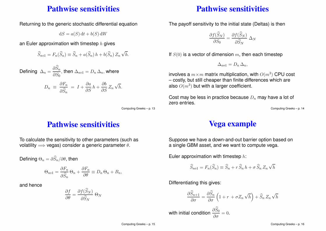
Pathwise sensitivities
Returning to the generic stochastic differential equation
dS = a(S) dt+ b(S) dW
an Euler approximation with timestep h gives
Sn+1 = Fn(Sn) ≡ Sn + a(Sn)h+ b(Sn)Zn
√h.
Defining ∆n =∂Sn
∂S0, then ∆n+1 = Dn∆n, where
Dn ≡ ∂Fn
∂Sn
= I +∂a
∂Sh+
∂b
∂SZn
√h.
Computing Greeks – p. 13
Pathwise sensitivities
The payoff sensitivity to the initial state (Deltas) is then
∂f(SN )
∂S0=
∂f(SN )
∂SN
∆N
If S(0) is a vector of dimension m, then each timestep
∆n+1 = Dn∆n,
involves a m×m matrix multiplication, with O(m3) CPU cost– costly, but still cheaper than finite differences which arealso O(m3) but with a larger coefficient.
Cost may be less in practice because Dn may have a lot ofzero entries.
Computing Greeks – p. 14
Pathwise sensitivities
To calculate the sensitivity to other parameters (such asvolatility =⇒ vegas) consider a generic parameter θ.
Defining Θn = ∂Sn/∂θ, then
Θn+1 =∂Fn
∂Sn
Θn +∂Fn
∂θ≡ DnΘn +Bn,
and hence∂f
∂θ=
∂f(SN )
∂SN
ΘN
Computing Greeks – p. 15
Vega example
Suppose we have a down-and-out barrier option based ona single GBM asset, and we want to compute vega.
Euler approximation with timestep h:
Sn+1 = Fn(Sn) ≡ Sn + r Sn h+ σ Sn Zn
√h
Differentiating this gives:
∂Sn+1
∂σ=
∂Sn
∂σ
(1 + r + σZn
√h)+ Sn Zn
√h
with initial condition∂S0
∂σ= 0.
Computing Greeks – p. 16
Vega example
Using the treatment discussed in Module 4, wherepn = pn(Sn, Sn+1, σ) is conditional probability of being acrossthe barrier in nth timestep, the discounted payoff is
exp(−rT ) (SN−K)+ PN
where
Pn =
n−1∏
m=0
(1− pm),
is probability of not crossing the barrier in first n timesteps,and P0 = 0.
Computing Greeks – p. 17
Vega example
SincePn+1 = Pn (1− pn)
then
∂Pn+1
∂σ=
∂Pn
∂σ(1−pn)−Pn
(∂pn
∂Sn
∂Sn
∂σ+
∂pn
∂Sn+1
∂Sn+1
∂σ+
∂pn∂σ
)
with initial condition∂P0
∂σ= 0.
The payoff sensitivity is then
exp(−rT )
(1SN>K
∂SN
∂σPN + (SN−K)+
∂PN
∂σ
)
Computing Greeks – p. 18
Automatic Differentiation
Generating the pathwise sensitivity code is tedious, butstraightforward, and can be automated:
source-source code generation: takes an old code forpayoff evaluation and produces a new code which alsocomputes sensitivities
operator overloading: defines new object (value +sensitivity), and re-defines operations appropriatelye.g. (
a
a
)∗(
b
b
)≡(
a b
a b+ a b
)
For more information, seewww.autodiff.org/people.maths.ox.ac.uk/gilesm/libor/
Computing Greeks – p. 19
Discontinuous payoffs
Pathwise sensitivity needs the payoff to be continuous.
What can you do when it is not?
for digital options, can use a crude piecewise linearapproximation
alternatively, use conditional expectations whicheffectively smooth the payoff
the barrier option is a good example of this, usingthe probability of crossing conditional on the pathvalues at discrete timesGlasserman discusses a similar approach for digitaloptions, stopping the path simulation one timestepearly then taking a conditional expectation
Computing Greeks – p. 20
Discontinuous payoffs
Glasserman’s approach has problems in multipledimensions (hard to evaluate expected value analytically)so I developed an approach I call “vibrato Monte Carlo”.
It is a hybrid method. Conditional on the path value SN−1
one timestep before the end, the value value SN has aNormal distribution, if using an Euler discretisation.
Hence, can use LRM for the final timetsep to get thesensitivity to changes in SN−1, and combine this withpathwise to get sensitivity of SN−1 to the input parameters.
M.B. Giles, ’Vibrato Monte Carlo sensitivities’, pp. 369-392in Monte Carlo and Quasi Monte Carlo Methods 2008,Springer, 2009. Computing Greeks – p. 21
Adjoint approach
The adjoint (or reverse mode AD) approach computes thesame values as the standard (forward) pathwise approach,but much more efficiently for the sensitivity of a singleoutput to multiple inputs.
The approach has a long history in applied math andengineering:
optimal control theory (find control which achievestarget and minimizes cost)
design optimization (find shape which maximizesperformance)
Computing Greeks – p. 22
Adjoint approach
Returning to the generic stochastic o.d.e.
dS = a(S) dt+ b(S) dW,
with Euler approximation
Sn+1 = Fn(Sn) ≡ Sn + a(Sn)h+ b(Sn)Zn
√h
if ∆n =∂Sn
∂S0, then ∆n+1 = Dn∆n, Dn ≡ ∂Fn(Sn)
∂Sn
,
and hence
∂f(SN )
∂S0=∂f(SN )
∂SN
∆N =∂f
∂SDN−1DN−2 . . . D0∆0
Computing Greeks – p. 23
Adjoint approach
If S is m-dimensional, then Dn is an m×m matrix,and the computational cost per timestep is O(m3).
Alternatively,
∂f(SN )
∂S0=
∂f
∂SDN−1DN−2 · · ·D0∆0 = V T
0 ∆0,
where adjoint Vn =
(∂f(SN )
∂Sn
)T
is calculated from
Vn = DTnVn+1, VN =
(∂f
∂SN
)T
,
at a computational cost which is O(m2) per timestep.Computing Greeks – p. 24
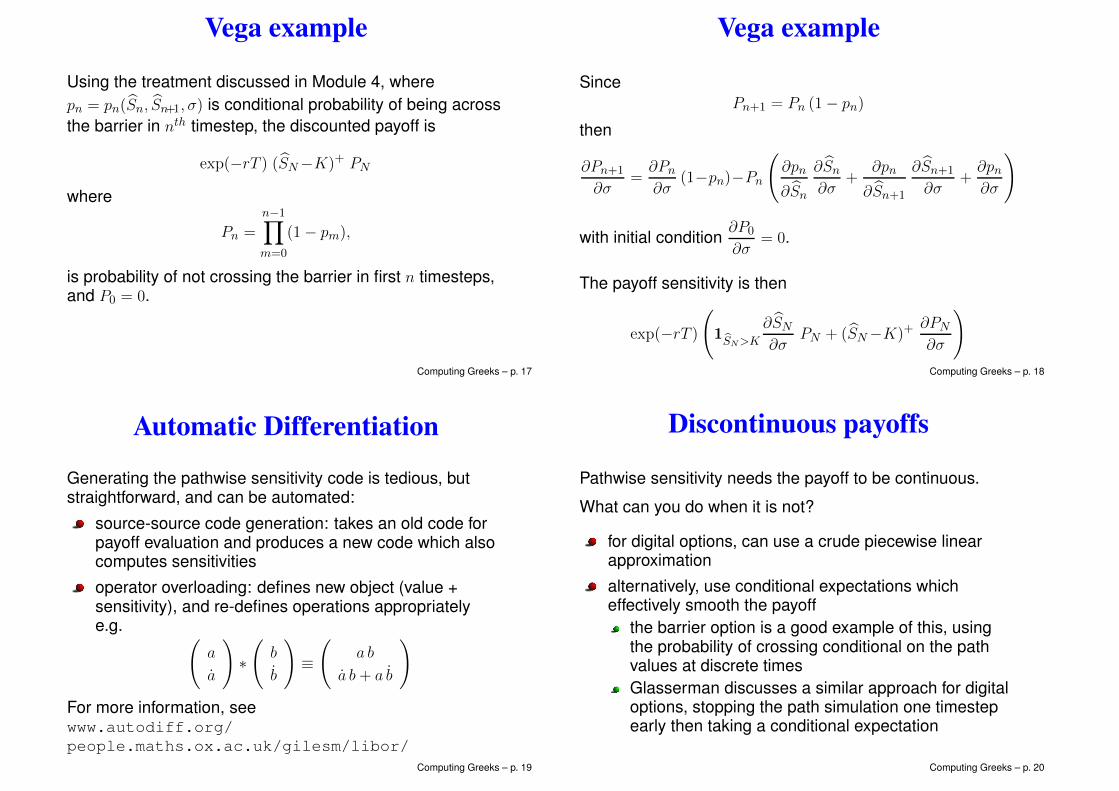
Adjoint approach
Note the flow of data within the path calculation:
S0 S1 . . . SN−1 SN
∂f/∂S
D0 D1 DN−1
V0 V1 . . . VN−1 VN
– memory requirements are not significant because dataonly needs to be stored for the current path.
Computing Greeks – p. 25
Adjoint approach
To calculate the sensitivity to other parameters, consider ageneric parameter θ. Defining Θn = ∂Sn/∂θ, then
Θn+1 =∂Fn
∂SΘn +
∂Fn
∂θ≡ DnΘn +Bn,
and hence
∂f
∂θ=
∂f
∂SN
ΘN
=∂f
∂SN
BN−1 +DN−1BN−2 + . . .
+DN−1DN−2 . . . D1B0
=
N−1∑
n=0
V Tn+1Bn.
Computing Greeks – p. 26
Adjoint approach
Different θ’s have different B’s, but same V ’s
=⇒ Computational cost ≃ m2 + m× # parameters,
compared to the standard forward approach for which
Computational cost ≃ m2 × # parameters.
However, the adjoint approach only gives the sensitivity ofone output, whereas the forward approach can give thesensitivities of multiple outputs for little additional cost.
Computing Greeks – p. 27
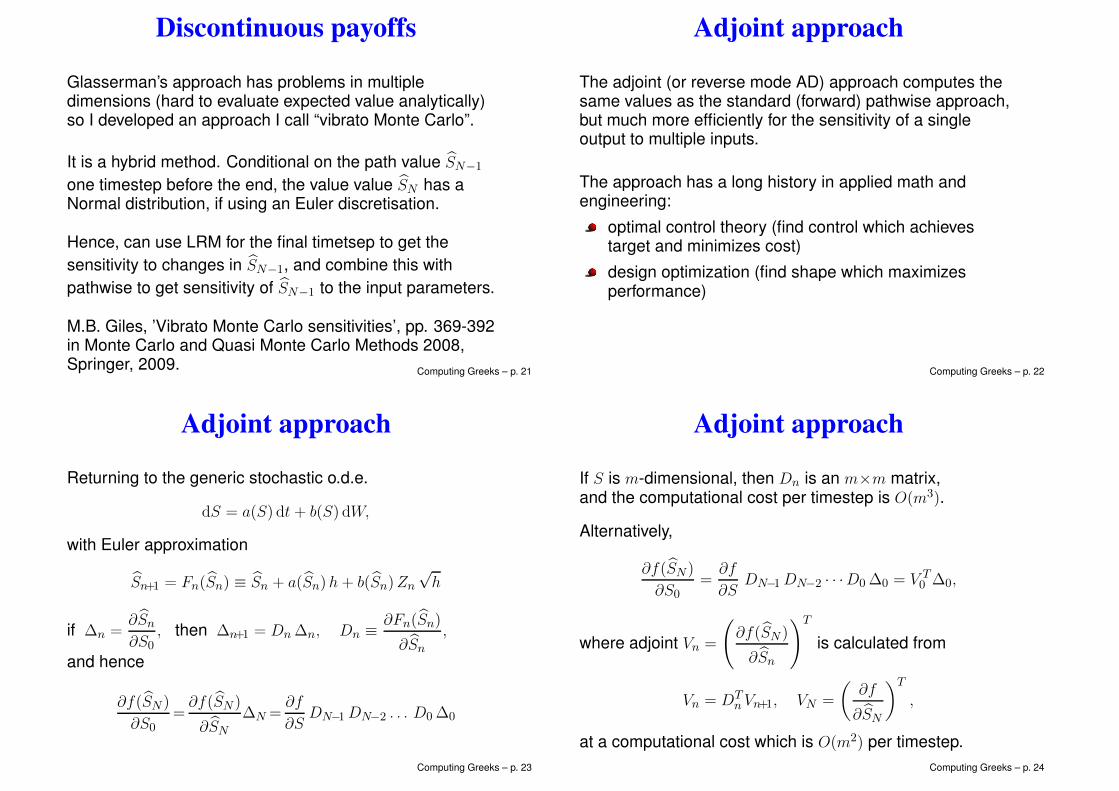
LIBOR Market Model
Finite differences versus forward pathwise sensitivities:
0 20 40 60 80 1000
50
100
150
200
250
Maturity N
rela
tive c
ost
finite diff deltafinite diff delta/vegapathwise deltapathwise delta/vega
Computing Greeks – p. 28
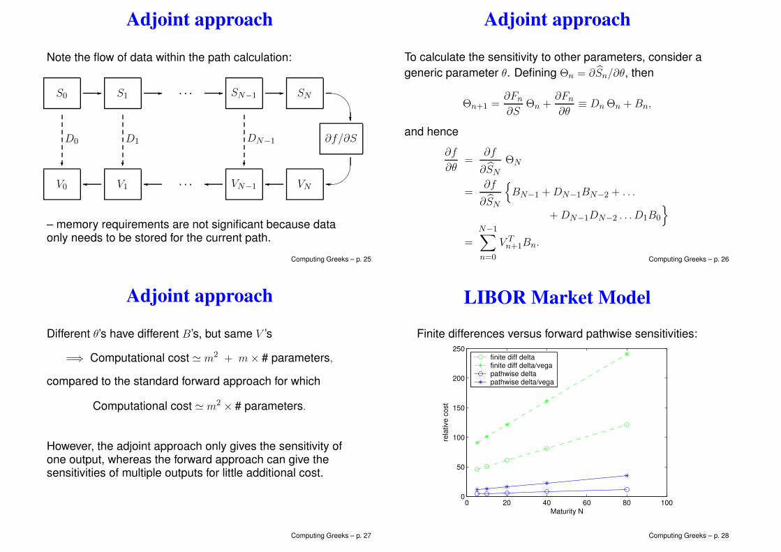
LIBOR Market Model
Forward versus adjoint pathwise sensitivities:
0 20 40 60 80 1000
5
10
15
20
25
30
35
40
Maturity N
rela
tive
co
st
forward deltaforward delta/vegaadjoint deltaadjoint delta/vega
Computing Greeks – p. 29
Conclusions
Greeks are vital for hedging and risk analysis
Finite difference approximation is simplest toimplement, but far from ideal
Likelihood ratio method for discontinuous payoffs
In all other cases, pathwise sensitivities are best
Payoff smoothing may handle the problem ofdiscontinuous payoffs
Adjoint pathwise approach gives an unlimited number ofsensitivities for a cost comparable to the initial valuation
Computing Greeks – p. 30
References
M.B. Giles, P. Glasserman. ’Smoking adjoints: fastMonte Carlo Greeks’, RISK, 19(1):88-92, January 2006.
M. Leclerc, Q. Liang, I. Schneider, ’Fast Monte CarloBermudan Greeks’, RISK, 22(7):84-88, 2009.
L. Capriotti, M.B. Giles. ’Fast correlation Greeks byadjoint algorithmic differentiation’, RISK, 23(4):77-83,2010.
L. Capriotti, J. Lee, M. Peacock, ’Real TimeCounterparty Credit Risk Management in Monte Carlo’,RISK 24(6):86-90, 2011.
L. Capriotti, ’Fast Greeks by algorithmic differentiation’,Journal of Computational Finance 14(3):3-35, 2011.
L. Capriotti, M.B. Giles. ’Algorithmic differentiation:adjoint Greeks made easy’, RISK, 25(10), 2012.Computing Greeks – p. 31