1-1

Advanced Design Application & Data Analysis for Field-Portable

XRF

Contact: Stephen Dyment, OSRTI/TIFSD, dyment.stephen@epa.gov

A Series of Web-based Seminars Sponsored by Superfund’s Technology Innovation & Field Services Division

1-2

How To . . .

Ask questions »“?” button on CLU-IN page

Control slides as presentation proceeds»manually advance slides

Review archived sessions»http://www.clu-in.org/live/arc

hive.cfm

Contact instructors

1-3

Module 1:

Introduction

1-4

Your Instructors…………….

Deana Crumbling - USEPA/OSRTI

» Technology Innovation Field Services Division

— crumbling.deana@epa.gov

Robert Johnson, PhD - Argonne National Lab

» Environmental Assessment Division

— rlj@anl.gov

Stephen Dyment - USEPA/OSRTI

» Technology Innovation Field Services Division

— dyment.stephen@epa.gov

1-5

Who Will Benefit from this Course?

Regulatory project managers and quality assurance reviewers who use XRF data

Consultants and regulatory staff responsible for

»Designing and approving work plans that use XRF

»Interpreting XRF data

1-6

Take Away Points…

Spatial heterogeneity is a primary source of data uncertainty

Traditional data strategies often not cost-effective for addressing this data uncertainty

More effective, efficient data designs involve » dynamic/adaptive field decision-making » real-time data generation and management tools

XRF is one of these tools Use of appropriate sampling designs, QA/QC, and

collaborative data allow higher certainty and defensible decisions with XRF

1-7

Web-Seminar Sessions and Schedule

Session 1» Module 1 - Introduction and Module 2 - XRF Basics» Monday, August 4, 2008. 1PM-3PM EST.» Stephen Dyment, Robert Johnson

Session 2 » Module 3.1 - Representativeness Part 1» Thursday, August 7, 2008. 1PM-3PM EST.» Deana Crumbling

Session 3 » Module 3.2 - Representativeness Part 2» Monday, August 11, 2008. 1PM-3PM EST.» Deana Crumbling (continued)

1-8

Web-Seminar Sessions and Schedule

Session 4 » Module 4, Demonstration of Method Applicability and QC» Thursday, August 14, 2008. 1PM-3PM EST.» Stephen Dyment

Session 5 » Module 5, XRF and Appropriate Quality Control Strategies» Monday, August 18, 2008. 1PM-3PM EST.» Stephen Dyment

Session 6 » Module 6.1 - Dynamic Work Strategies Part 1» Thursday, August 21, 2008. 1PM-3PM EST.» Robert Johnson

(continued)

1-9

Web-Seminar Sessions and Schedule

Session 7

» Module 6.2 - Dynamic Work Strategies Part 2

» Monday, August 25, 2008. 1PM-3PM EST.

» Robert Johnson

Session 8

» Q&A for Session 7, In Depth Q&A Review for All Seminars, and Resources

» Thursday, August 28, 2008. 1PM-3PM EST.

» Deana Crumbling, Robert Johnson, Stephen Dyment

1-10

Session Logistics

Each session will be 2 hours long

Questions should be submitted by email or chat

Some questions may be answered at the end of the current session

Most questions will be answered during the first 30 minutes of the subsequent session

1-11

Session Breakouts

Session 1» Presentation» Answers to some questions

Session 2 through 7» 30 minutes answering questions submitted for previous

session» 1 hour and 30 minute presentation for current session» Answers to some questions for current session

Session 8» 30 minutes answering questions submitted for

Session 7» Q&A review for Sessions 1 - 7» Review of resources

1-12

Instrument and Software DisclaimerReferring to specific XRF instruments or software packages is for information purposes only and does constitute endorsement.

Manufacturers Niton and Innov-X Excel (Microsoft Office) Visual Sampling Plan (Pacific Northwest Lab: http://

dqo.pnl.gov/) BAASS (Argonne National Lab: http://

www.ead.anl.gov/project/dsp_topicdetail.cfm?topicid=23) Surfer/Grapher (Golden Software:

www.goldensoftware.com ) ArcView 3.x or 9.x (ESRI: www.esri.com) Freeware can be found at

http://www.frtr.gov/decisionsupport/

Module 2:

Basic XRF Concepts

2-1

What Does An XRF Measure?

X-ray source irradiates sample

Elements emit characteristic x-rays in response

Characteristic x-rays detected

Spectrum produced (frequency and energy level of detect x-rays)

Concentration present estimated based on sample assumptions

2-2

So

urce

: h

ttp://o

me

ga

.ph

ysics.uo

i.gr/xrf/e

ng

lish/im

ag

es/P

RIN

CIP

.jpg

Example XRF Spectra

2-3

Bench-top XRF

2-4

How is an XRF Typically Used?

Measurements on prepared samples

Measurements through bagged samples (limited preparation)

In situ measurements of exposed surfaces

2-5(continued)

How is an XRF Typically Used?

Measurements on prepared samples

Measurements through bagged samples (limited preparation)

In situ measurements of exposed surfaces

2-6

What Does an XRF Typically Report?

Measurement date

Measurement mode

“Live time” for measurement acquisition

Concentration estimates

Analytical errors associated with estimates

User defined fields

2-7

Which Elements Can An XRF Measure?

Generally limited to elements with atomic number > 16

Method 6200 lists 26 elements as potentially measurable

XRF not effective for lithium, beryllium, sodium, magnesium, aluminum, silicon, or phosphorus

In practice, interference effects among elements can make some elements “invisible” to the detector, or impossible to accurately quantify

2-8

How Is An XRF Calibrated?

Fundamental Parameters Calibration – calibration based on known detector response properties, “standardless” calibration, what is commonly done

Empirical Calibration – calibration calculated using regression analysis and known standards, either site-specific media with known concentrations or prepared, spike standards

2-9

In both cases, the instrument will have a dynamic range over which a linear calibration is assumed to hold.

Dynamic Range a Potential Issue

No analytical method is good over the entire range of concentrations potentially encountered with a single calibration

XRF typically under-reports concentrations when calibration range has been exceeded

Primarily an issue with risk assessments

2-10

Figure 1: ICP vs XRF (lead - all data)

y = 0.54x + 200

R2 = 0.95

0

500

1000

1500

2000

2500

3000

3500

4000

4500

5000

0 2000 4000 6000 8000 10000

ICP Lead ppm

XR

F L

ead

pp

m

Standard Innov-X Factory Calibration List

Antimony (Sb) Iron (Fe) Selenium (Se)

Arsenic (As) Lead (Pb) Silver (Ag)

Barium (Ba) Manganese (Mn) Strontium (Sr)

Cadmium (Cd) Mercury (Hg) Tin (Sn)

Chromium (Cr) Molybdenum (Mo) Titanium (Ti)

Cobalt (Co) Nickel (Ni) Zinc (Zn)

Copper (Cu) Rubidium (Ru) Zirconium (Zr)

2-11

How Is XRF Performance Commonly Defined?

Bias – does the instrument systematically under or over-estimate element concentrations?

Precision – how much “scatter” solely attributable to analytics is present in repeated measurements of the same sample?

Detection Limits – at what concentration can the instrument reliably identify the presence of an element?

Quantitation Limits – at what concentration can the instrument reliably measure an element?

Representativeness – how representative is the XRF result of information required to make a decision?

Comparability – how do XRF results compare with results obtained using a standard laboratory technique?

2-12

Analytical Precision Driven By…

Measurement time – increasing measurement time reduces error

Element concentration present – increasing concentrations increase error

Concentrations of other elements present – as other element concentrations rise, general detection limits and errors rise as well

2-13

Lead Example: Concentration Effect

2-14

Reported Error vs. Lead Concentrations

0

10

20

30

40

50

60

70

80

0 500 1000 1500 2000 2500 3000

XRF Lead Concentrations (ppm)

Rep

ort

ed E

rro

r (p

pm

)

Lead Example: Concentration Effect

2-15

% Error vs. Lead Concentrations

0

5

10

15

20

25

30

35

0 500 1000 1500 2000 2500 3000

XRF Lead Concentrations (ppm)

% E

rro

r

XRF Detection Limit (DL) Calculations

SW-846 Method 6200 defines DL as 3 X the standard deviation (SD) attributable to the analytical variability (imprecision) at a low concentration

XRF “measures” by counting X-ray pulsesXRF instruments typically report DLs based on

counting statistics using the 3 X SD definitionSDs and associated DLs can also be calculated

manually from repeated measurements of a sample (if concentrations are detectable to begin with)

2-16

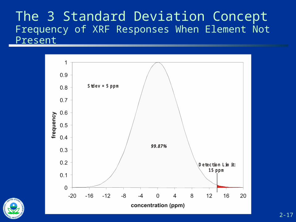
The 3 Standard Deviation ConceptFrequency of XRF Responses When Element Not Present

2-17

Stdev = 5 ppm

Detection Lim it:15 ppm

99.87%

DL <> Reliable Detection

2-18

Stdev = 5 ppm

DL <> Reliable Detection

2-19

Stdev = 5 ppm

DL <> Reliable Detection

2-20

Stdev = 5 ppm

For Any Particular Instrument, Detection Limits Are Influenced By…

Measurement time (quadrupling time cuts detection limits in half)

Matrix effects

Presence of interfering or highly elevated contamination levels

Consequently, the DL for any particular element will change, sometimes dramatically, from one sample to the next, depending on sample characteristics and operator choices

2-21

Examples of DL…

AnalyteInnov-X1

120 sec acquisition(soil standard – ppm)

Innov-X1

120 sec acquisition(alluvial deposits - ppm)

Innov-X1

120 sec acquisition(elevated soil - ppm)

Antimony (Sb) 61 55 232

Arsenic (As) 6 7 29,200

Barium (Ba) NA NA NA

Cadmium (Cd) 34 30 598

Calcium (Ca) NA NA NA

Chromium (Cr) 89 100 188,000

Cobalt (Co) 54 121 766

Copper (Cu) 21 17 661

Iron (Fe) 2,950 22,300 33,300

Lead (Pb) 12 8 447,000

Manganese (Mn) 56 314 1,960

Mercury (Hg) 10 8 481

Molybdenum (Mo) 11 9 148

Nickel (Ni) 42 31 451

2-22

To Report, or Not to Report: That is the Question!

Not all instruments/software allow the reporting of XRF results below detection limits

For those that do, manufacturer often recommends against doing it

Can be valuable information if careful about its use…particularly true if one is trying to calculate average values over a set of measurements

2-23

XRF Data Comparability

Comparability usually refers to comparing XRF results with standard laboratory data

Assumption is one has samples analyzed by both XRF and laboratory

Regression analysis is the ruler most commonly used to measure comparability

SW-846 Method 6200: “If the r2 is 0.9 or greater…the data could potentially meet definitive level data criteria.”

2-24

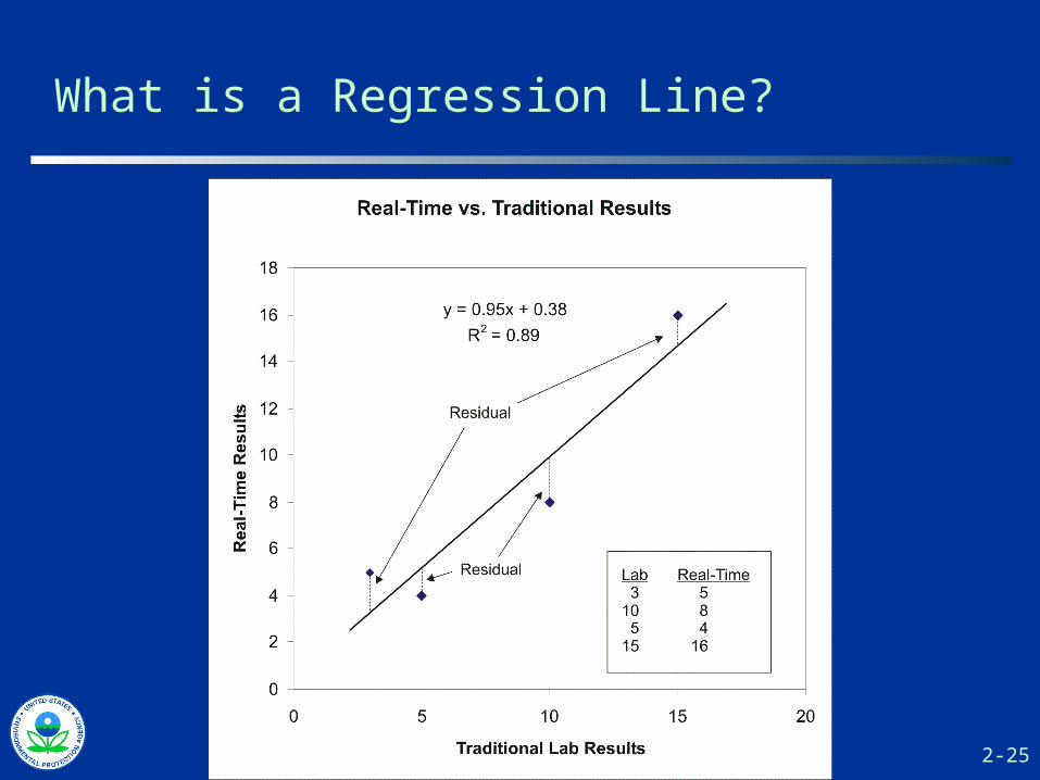
What is a Regression Line?

2-25

Regression Terminology

Scatter Plot: graph showing paired sample results Independent Variable: x-axis values Dependent Variable: y-axis values Residuals: difference between dependent variable result

predicted by regression line and observed dependent variable

Adjusted R2: a measure of goodness-of-fit of regression line

Homoscedasticity/Heteroscedasticity: Refers to the size of observed residuals, and whether this size is constant over the range of the independent variable (homoscedastic) or changes (heteroscedastic)

2-26

Heteroscedasticity is a Fact of Life for Environmental Data Sets

2-27

Appropriate Regression Analysis

Based on paired analytical results, ideally from same sub-sample

Paired results focus on concentration ranges pertinent to decision-making

Non-detects are removed from data set

Best regression results obtained when pairs are balanced at opposite ends of range of interest

2-28

Evaluating Regression Performance

No evidence of inexplicable “outliers”

Balanced data sets

No signs of correlated residuals

High R2 values (close to 1)

Constant residual variance (homoscedastic)

2-29

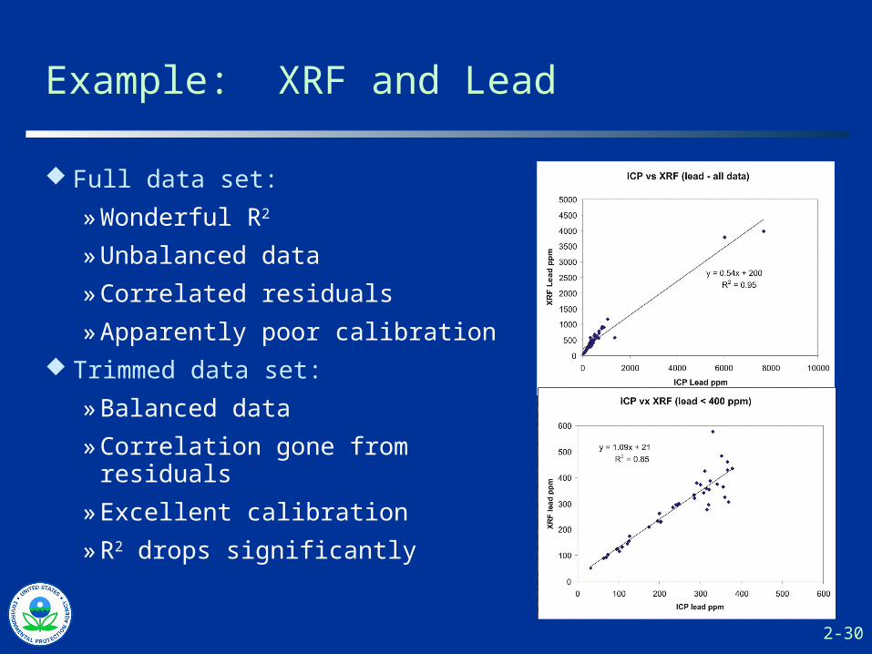
Example: XRF and Lead

Full data set:

» Wonderful R2

» Unbalanced data

» Correlated residuals

» Apparently poor calibration

Trimmed data set:

» Balanced data

» Correlation gone from residuals

» Excellent calibration

» R2 drops significantly

2-30

Converting XRF Data for Risk Assessment Use

Purpose: making XRF data “comparable” to lab data for risk assessment purposes

To consider:» Need for “conversion” may be an indication of a bad

regression» XRF calibrations not linear over the range of concentrations

potentially encountered» Extra variability in XRF data not an issue (captured in UCL

calculations when estimating EPC)» Contaminant concentration distributions are typically

skewed… lots of XRF data may provide a better UCL/EPC estimate than a few lab results even if the regression is not great

2-31

A Cautionary Example…

Four lab lead results: 20, 24, 86, and 189 ppmProUCL 95%UCL Calculations:

»Normal: 172 ppm»Gamma: 434 ppm»Lognormal: 246 – 33,835 ppm»Non-parametric: 144 – 472 ppm

Four samples are not enough to either understand the variability present, or the underlying contamination distribution

2-32

Will the “Definitive” Data Please Stand Up?

One of these scatter plots shows the results of arsenic from two different ICP labs, and the other compares XRF and ICP arsenic results.

Which is which?

2-33

Definitive Data, Please Stand Up!

2-34

Take-Away Comparability Points

Standard laboratory data can be “noisy” and are not necessarily an error-free representation of reality

Regression R2 values are a poor measure of comparability

Focus should be on decision comparability, not laboratory result comparability

Examine the lab duplicate paired results from traditional QC analysis - The split field vs. lab regression cannot be expected to be better than the lab’s duplicate vs. duplicate regression

2-35

What Affects XRF Performance?

Measurement time – the longer the measurement, the better the precision

Contaminant concentrations – potentially outside calibration ranges, absolute error increases, enhanced interference effects

Sample preparation – the better the sample preparation, the more likely the XRF result will be representative

2-36(continued)

What Affects XRF Performance?

Interference effects – the spectral lines of elements may overlap

Matrix effects – fine versus coarse grain materials may impact XRF performance, as well as the chemical characteristics of the matrix

Operator skills – watching for problems, consistent and correct preparation and presentation of samples

2-37

What Are Common XRF Environmental Applications?

In situ and ex situ analysis of soil samples

Ex situ analysis of sediment samples

Swipe analysis for removable contamination on surfaces

Filter analysis for filterable contamination in air and liquids

Lead-in-paint applications

2-38

Recent XRF Technology Advancements…

Miniaturization of electronics

Improvements in detectors

Improvements in battery life

Improved electronic x-ray tubes

Improved mathematical algorithms for interference corrections

Bluetooth, coupled GPS, connectivity with PDAs and tablet computers

2-39

…Contribute to Steadily Improving Performance

AnalyteDL in Quartz Sand by

Method 6200 (600 sec – ppm)

TN 900 (60 to 100 sec) – ppm

Innov-X1

120 sec acquisition(soil standard – ppm)

Antimony (Sb) 40 55 61

Arsenic (As) 40 60 6

Barium (Ba) 20 60 NA

Cadmium (Cd) 100 NA 34

Chromium (Cr) 150 200 89

Cobalt (Co) 60 330 54

Copper (Cu) 50 85 21

Iron (Fe) 60 NA 2,950

Lead (Pb) 20 45 12

Manganese (Mn) 70 240 56

Mercury (Hg) 30 NA 10

Molybdenum (Mo) 10 25 11

Nickel (Ni) 50 100 422-40

Q&A – If Time Allows

2-41

After viewing the links to additional resources, please complete our online feedback form.

Thank You

Links to Additional ResourcesLinks to Additional Resources

Feedback FormFeedback Form

Thank You

2-42