Embed Size (px)
Citation preview
3.2-1
Advanced Design Application & Data Analysis for Field-Portable
XRF
Contact: Stephen Dyment, OSRTI/TIFSD, [email protected]
A Series of Web-based Seminars Sponsored by Superfund’s Technology Innovation & Field Services Division
3.2-2
How To . . .
Ask questions »“?” button on CLU-IN page
Control slides as presentation proceeds»manually advance slides
Review archived sessions»http://www.clu-in.org/live/arc
hive.cfm
Contact instructors
3.2-3
Q&A For Session 1 – Introduction and Basic XRF Concepts
3.2-4
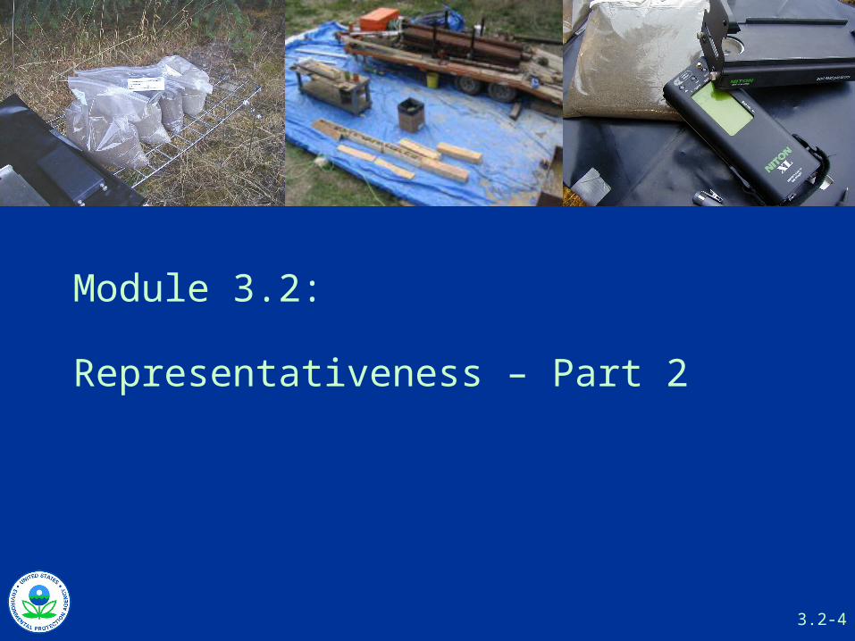
Module 3.2:
Representativeness – Part 2
3.2-5
Review: Sample Representativeness
“A representative sample is one that answers a question about a population with a given confidence.”
“A sample that is representative for a specific question is most likely not representative for a different question.”
From Ramsey & Hewitt, “A Methodology for Assessing Sample Representativeness,” published in Environmental Forensics (2005)
Also quoted in SW-846 Method 8330B (App A.1.3 p. A-6)
3.2-6
Sample Support is the Foundation of Sample Representativeness
Module 3.1 explained what sample support is and why it is so critical to data quality
Controlling sample support helps reduce the effects of micro-scale (within-sample) and short-scale (between-samples) matrix heterogeneity
Sample support MUST ABSOLUTELY be controlled when splitting samples to assess analytical method comparability
3.2-7
Fictional Example of a “Support Chain” for Grab Samples: Step 1
Determine the Decision Support Clarify project decision: Determine average conc of metal
analyte (Me) over a decision unit defined according to the data needs of the eco-risk assessor
The eco-risk assessor has defined the decision unit as an exposure unit, which is the soil encompassed by a 1-acre area and 1-ft depth. Relevant eco-receptors are assumed to be equally exposed to all soil particle sizes.
So, the decision support = 1-acre soil area (2-dimensions) from 0 to 12-in depth (3rd dimension). The total Me conc for the bulk soil is assumed to be representative of receptor exposure to Me. EPC* will be calculated over this decision support.
3.2-8
“Support Chain” Fictional Illustration: Step 2
Determine the Desired Degree of Data Confidence & Develop the Preliminary CSM
For input into the risk equations, the risk assessor would like to have a 95% UCL for the exposure unit that is within +10% of the calculated mean
Preliminary CSM: Release of Me to exposure unit occurred 10 yrs ago when a nearby lagoon overflowed onto this flat meadow area. So the distribution of Me is expected to be reasonably homogeneous at a macro-scale across the exposure area. An initial guesstimate of the true mean is in the vicinity of 300-400.
3.2-9
“Support Chain” Fictional Illustration: Step 3
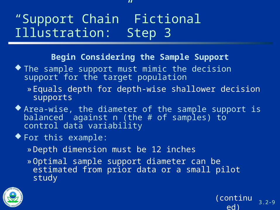
Begin Considering the Sample Support The sample support must mimic the decision support for the
target population
» Equals depth for depth-wise shallower decision supports Area-wise, the diameter of the sample support is balanced
against n (the # of samples) to control data variability For this example:
» Depth dimension must be 12 inches
» Optimal sample support diameter can be estimated from prior data or a small pilot study
(continued)
3.2-10
“Support Chain” Fictional Illustration: Step 3
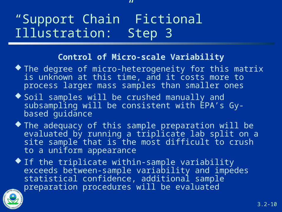
Control of Micro-scale Variability The degree of micro-heterogeneity for this matrix is
unknown at this time, and it costs more to process larger mass samples than smaller ones
Soil samples will be crushed manually and subsampling will be consistent with EPA’s Gy-based guidance
The adequacy of this sample preparation will be evaluated by running a triplicate lab split on a site sample that is the most difficult to crush to a uniform appearance
If the triplicate within-sample variability exceeds between-sample variability and impedes statistical confidence, additional sample preparation procedures will be evaluated
3.2-11
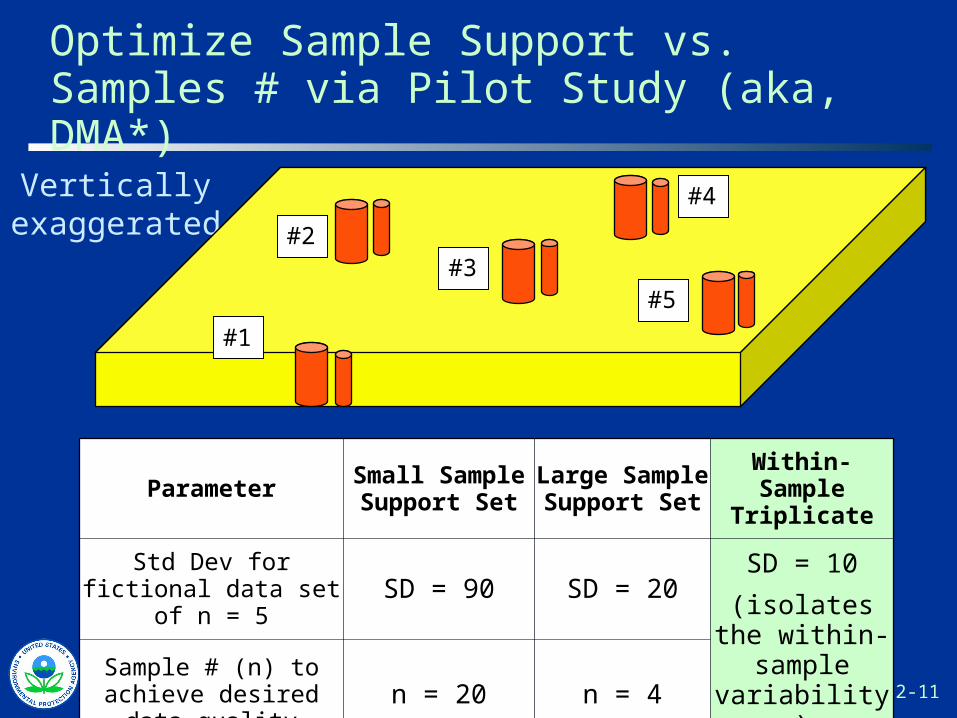
Optimize Sample Support vs. Samples # via Pilot Study (aka, DMA*)
Vertically exaggerated
#1
#4
#5#3
#2
ParameterSmall Sample Support Set
Large Sample Support Set
Within-Sample Triplicate
Std Dev for fictional data set of n = 5 SD = 90 SD = 20 SD = 10
(isolates the within-sample
variability)Sample # (n) to achieve
desired data quality n = 20 n = 4
3.2-12
“Support Chain” Fictional Illustration: Step 4
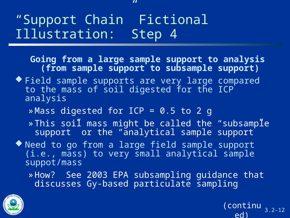
Going from a large sample support to analysis(from sample support to subsample support)
Field sample supports are very large compared to the mass of soil digested for the ICP analysis» Mass digested for ICP = 0.5 to 2 g» This soil mass might be called the “subsample support”
or the “analytical sample support” Need to go from a large field sample support (i.e., mass)
to very small analytical sample suppot/mass » How? See 2003 EPA subsampling guidance that
discusses Gy-based particulate sampling
(continued)
3.2-13
“Support Chain” Fictional Illustration: Step 4
Representative Subsampling Options for our fictional story
» Grind large samples to uniform particle size and take ~1 g subsample
— Equipment able to efficiently grind large sample masses might not be readily available
» Use Gy-based sample handling to progressively subsample in a representative way
— Reduces sample mass to a small subsample that is easily ground
— Take 1-g for analysis
3.2-14
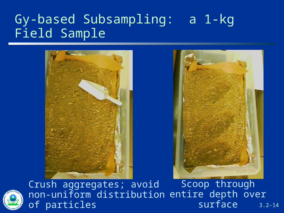
Gy-based Subsampling: a 1-kg Field Sample
Crush aggregates; avoid non-uniform distribution of particles
Scoop through entire depth over surface
3.2-15
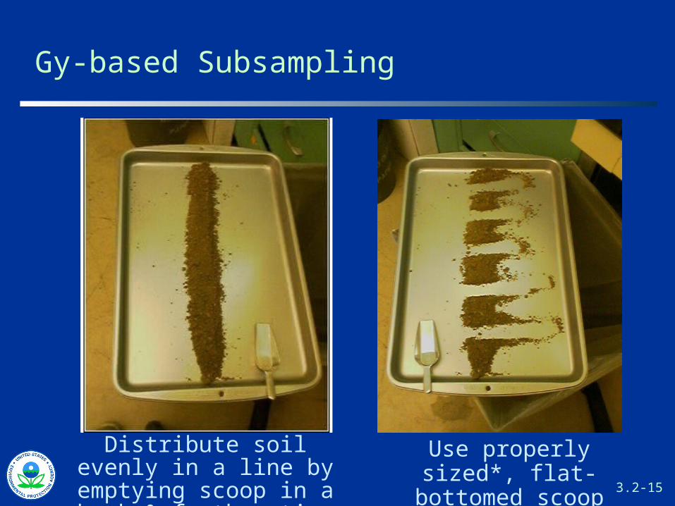
Gy-based Subsampling
Distribute soil evenly in a line by emptying scoop in a
back & forth motion
Use properly sized*, flat-bottomed scoop
3.2-16
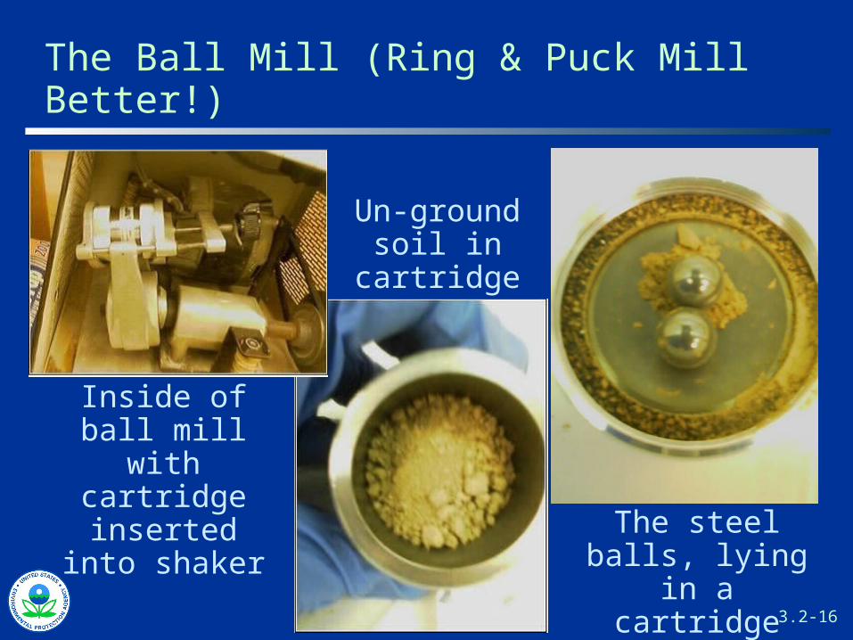
The Ball Mill (Ring & Puck Mill Better!)
Inside of ball mill with cartridge
inserted into shaker
Un-ground soil in
cartridge
The steel balls, lying in a
cartridge cap
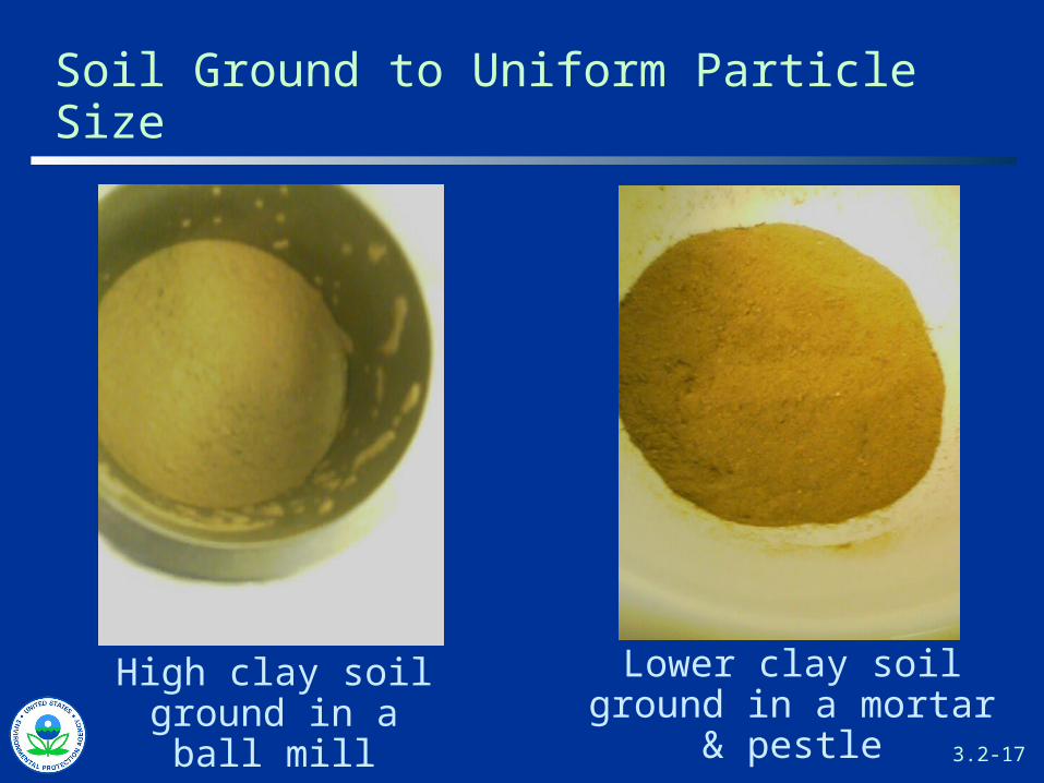
3.2-17
Soil Ground to Uniform Particle Size
High clay soil ground in a ball mill
Lower clay soil ground in a mortar & pestle
3.2-18
“Support Chain” Fictional Illustration: Step 5
Measurement Support
The analytical instrument “sees” only what is injected into it in liquid form
Analytical sample preparation
» Digestion or extraction must be appropriate for (i.e., be representative of) the parameter of interest.
ICP* metals analysis does not always report total metals
» Digestion w/ nitric acid does not solubilize all of the minerals that may be binding metals in the soil matrix
» Certain metals routinely recover poorly (e.g., antimony)
3.2-19
Quick Review
Control sample support to reduce within- and between-sample heterogeneity:
» improves data quality
» reduces data variability
» reduces incidence of “outliers”
Sample support MUST be controlled when splitting samples
Controlling sample support increases agreement between field and lab duplicates which improves QC
» QC is a mechanism to estimate data uncertainty
3.2-20
Review of “Supports”
Decision Unit Support - the spatial dimensions and other physical properties (such as particle size) that define the population of interest targeted by the decision.
Sample Support - the spatial dimensions and other physical properties (such as particle size) of a physical sample; it needs to be selected to mirror the decision unit support.
Measurement Support - the choice of analytical sample preparation (laboratory subsampling & digestion/ extraction prior to instrumental measurement) that determines how much of the original sample content is actually “seen” and measured by the instrument
3.2-21
Question:Why do we need to understand all this?
Answer
Because XRF analytical programs perform much, much, MUCH better when XRF sampling and
analysis designs apply this knowledge
Let’s talk about the supports relevant to field-portable XRF instrumentation
3.2-22
XRF’s “Supports”
Analytical Sample Support» The X-rays pass thru a window that is only a few cm2 in
area— They penetrate 1 - 2 mm depth into the soil surface— The instrument “sees” ~ 2 g or less of a thin soil
layer» Soil particle size and its correlation to Me concentration
determines how much Me is in the XRF’s field of view Measurement support (same as analytical sample
support)» XRF measures the total element content of the soil
volume for analytes it sees
3.2-23
Measurement support: XRF vs. ICP
ICP analysis requires digestion of soil mineral structure to free metals into solution» The common nitric acid (HNO3) digestion does not free
all metal present in the sample. How much is solubilized depends on soil mineralogy, the metal species released and how long ago, the redox and pH soil environment over the years…
» Hydrofluoric acid (HF) digests all minerals so total metal is measured by ICP analysis - but it is hard to find environmental labs with HF capability
XRF directly measures total metals» Results more comparable to HF digestion
3.2-24
Controlling XRF Sample Support
XRF’s small sample support (1-2 grams, on the order of a lab subsample) makes it susceptible to non-representative readings (i.e., readings that are very different from the average concentration of the sample)
The more uniform the distribution of soil particles, the more precise the XRF readings
Uniformity depends on the adequacy of sample handling and preparation
3.2-25
XRF Sample Handling/Preparation
There are 3 main types of sample preparation for XRF— the effectiveness of all is influenced by operator effort and consistency
Sample handling procedures should be defined in detail in the QAPP and followed meticulously»Prepare soil for in situ “shots”»Taking shots (i.e., readings) over a bagged
sample»Taking shots on a cup containing highly
prepared soil
3.2-26
Sample Preparation Option 1: in situ
Grades of sample preparation for in situ “shots”
» Least preparation: “shoot” on bare ground with minimal debris removal & smoothing
» Most preparation: Loosen soil to selected depth of interest. Carefully pick out extraneous material. Crush & mix soil in situ until uniform appearance. Smooth/compress surface before placing XRF.
» Take several shots in the same prepared location. Re-position the XRF between shots to estimate matrix variability (evaluate the adequacy of sample prep)
3.2-27
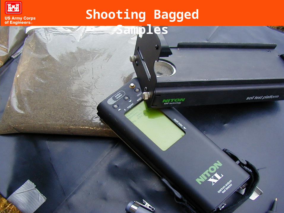
Sample Preparation Option 2: Bagged
Bagged samples» Increases sample support compared to in situ shots,
especially when multiple shots are taken per bag» Remove extraneous material. If necessary, crush soil
before placing into bag (crushing a hard soil in a bag can damage the smoothness of the plastic).
» Mix bag by kneading (also breaks up aggregates) and/or turn bag end-over-end. Visually inspect to ensure uniform appearance. Do not just shake bag—will cause particle segregation and increase data variability.
» Do not shoot through significant dimples or creases in the plastic—can cause increased reading variability
3.2-28 January 2008 XRF Applications Seminar 28
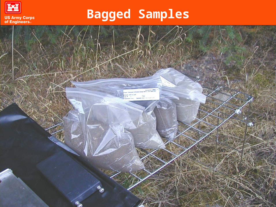
Bagged Samples
3.2-29 January 2008 XRF Applications Seminar 29
Shooting Bagged Samples
3.2-30
Benefits of Bagged Samples
When sampled from 1 sampling location, bagged samples increase the sample support from that location (this strategy controls within-sample variability)
Multi-increment sampling can be performed: Placing increments from across the decision unit into 1 bag further increases the sample support and is more representative of the decision unit average (this controls for short-scale matrix variability)
Taking multiple shots over the bag estimates the degree of within-sample variability (particle size effects) and the statistical average of those readings provides a better estimate of the true concentration for the bag
(continued)
3.2-31
Benefits of Bagged Samples
Sample bagging and readings can be performed in real-time» The number of shots over the bag can be adjusted in
real-time (either up or down) to provide statistically valid results
» Within-bag variability that is too high can be addressed by additional kneading or other corrective actions, or by examination of bag (ex: paint chips?)
» Inexpensive» Supports dynamic work strategy for field work by
providing data of known and documented quality
3.2-32
Sample Preparation Option 3: XRF Cups
Cup samples
» Remove debris, dry, grind, and sieve to achieve uniform particle size
» Subsample properly and place into XRF cups
» Be CAREFUL tapping cups if particle size not completely uniform—will segregate fines.
Highest homogeneity = best precision
» Best for determining method comparability to ICP or AA
» Perform XRF and ICP/AA analysis on same cup
3.2-33
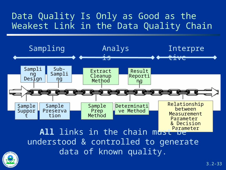
Data Quality Is Only as Good as the Weakest Link in the Data Quality Chain
Sampling Analysis Interpretive
Sample Support
Sampling Design
Sample Preservation
Sub-Sampling
Sample Prep Method
Determinative Method
Result Reporting
Extract CleanupMethod
Relationship between Measurement Parameter
& Decision Parameter
All links in the chain must be understood & controlled to generate data of known quality.
3.2-34
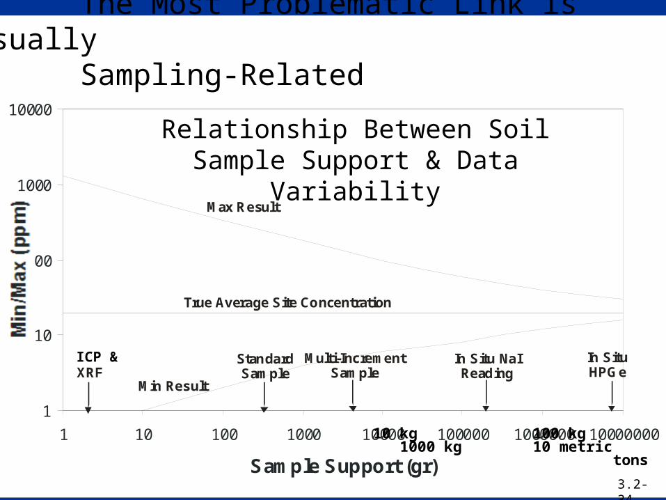
Range of Results vs Sample Support
1
10
100
1000
10000
1 10 100 1000 10000 100000 1000000 10000000
Sample Support (gr)
Min
/Ma
x (p
pm
)
True Average Site Concentration
Max Result
Min ResultXRF
StandardSample
Multi-IncrementSample
In Situ NaIReading
In SituHPGe
10 kg 100 kg 1000 kg 10 metric tons
The Most Problematic Link is Usually Sampling-Related
ICP &
Relationship Between Soil Sample Support & Data Variability
3.2-34
3.2-35 January 2008 XRF Applications Seminar 35
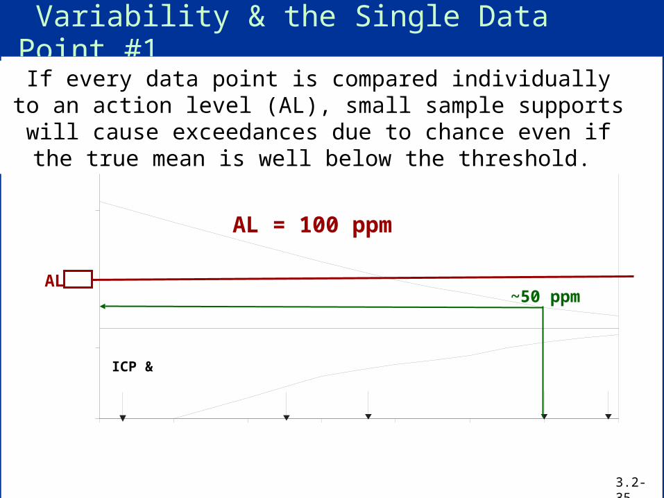
Variability & the Single Data Point #1
~50 ppm
If every data point is compared individually to an action level (AL), small sample supports will cause exceedances due to chance even if the true mean is well below the threshold.
ICP &
AL
AL = 100 ppm
3.2-35
3.2-36 January 2008 XRF Applications Seminar 36
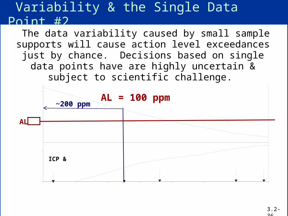
Variability & the Single Data Point #2
~200 ppm
The data variability caused by small sample supports will cause action level exceedances just by chance. Decisions
based on single data points have are highly uncertain & subject to scientific challenge.
ICP &
AL
AL = 100 ppm
3.2-36
3.2-37
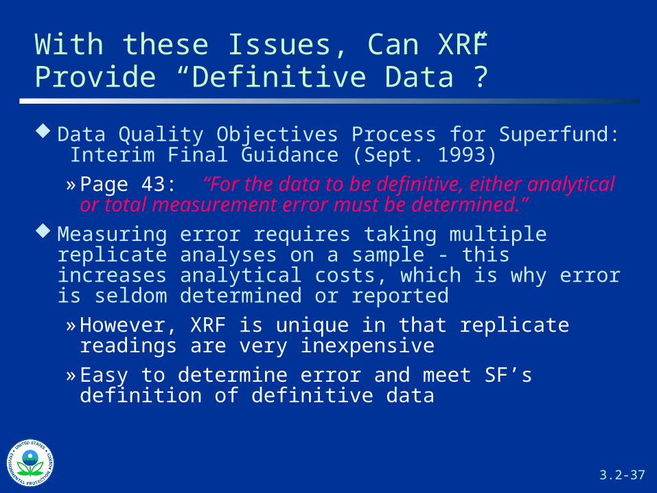
With these Issues, Can XRF Provide “Definitive Data”?
Data Quality Objectives Process for Superfund: Interim Final Guidance (Sept. 1993)» Page 43: “For the data to be definitive, either analytical
or total measurement error must be determined.” Measuring error requires taking multiple replicate
analyses on a sample - this increases analytical costs, which is why error is seldom determined or reported» However, XRF is unique in that replicate readings are
very inexpensive» Easy to determine error and meet SF’s definition of
definitive data
3.2-38
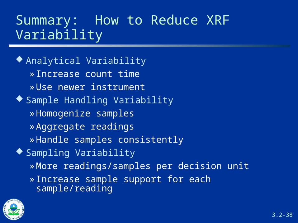
Summary: How to Reduce XRF Variability
Analytical Variability » Increase count time» Use newer instrument
Sample Handling Variability» Homogenize samples» Aggregate readings» Handle samples consistently
Sampling Variability» More readings/samples per decision unit» Increase sample support for each sample/reading
3.2-39
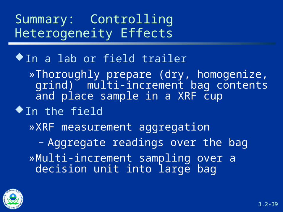
Summary: Controlling Heterogeneity Effects
In a lab or field trailer»Thoroughly prepare (dry, homogenize, grind)
multi-increment bag contents and place sample in a XRF cup
In the field»XRF measurement aggregation
—Aggregate readings over the bag»Multi-increment sampling over a decision unit
into large bag
3.2-40
How Many Increments?
Addressed in Module 6
3.2-41
Q&A – If Time Allows

After viewing the links to additional resources, please complete our online feedback form.
Thank You
Links to Additional ResourcesLinks to Additional Resources
Feedback FormFeedback Form
Thank You
3.2-42