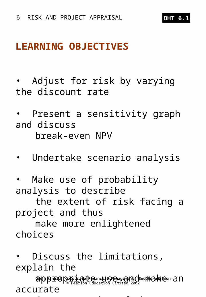
Adjust for risk by varying the discount rate Present a sensitivity graph and discuss

6 RISK AND PROJECT APPRAISAL

Glen Arnold: Corporate Financial Management, Second edition© Pearson Education Limited 2002

OHT 6.1

• Adjust for risk by varying the discount rate • Present a sensitivity graph and discuss break-even NPV • Undertake scenario analysis • Make use of probability analysis to describe the extent of risk facing a project and thus make more enlightened choices • Discuss the limitations, explain the appropriate use and make an accurate interpretation of the results of the four risk techniques described in this chapter

LEARNING OBJECTIVES



OHT 6.2

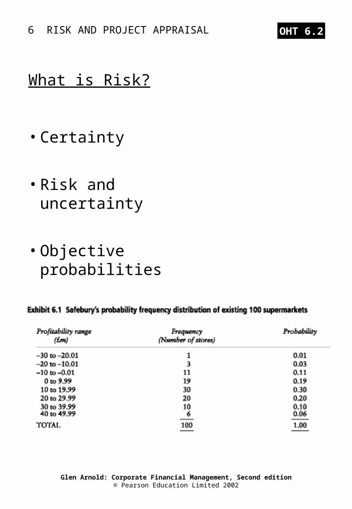
What is Risk?

• Certainty

• Risk and uncertainty

• Objective probabilities

• Subjective probabilities



OHT 6.3



OHT 6.4

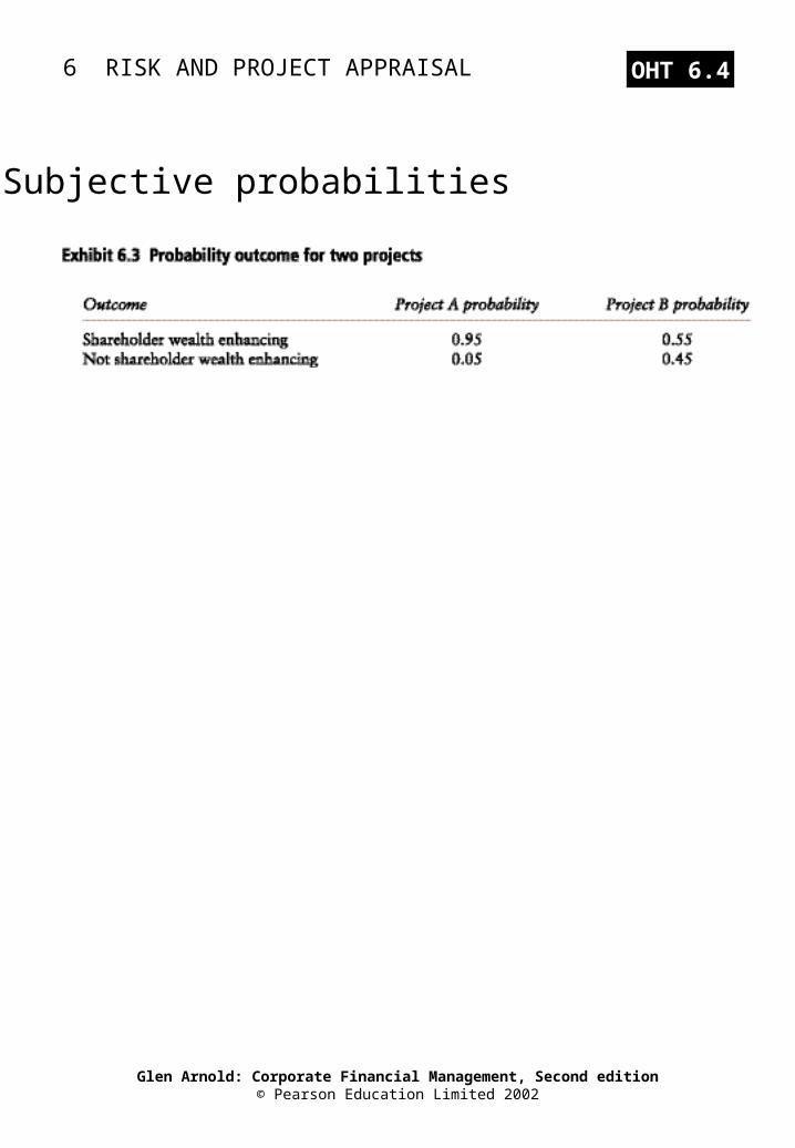
• Subjective probabilities



OHT 6.5

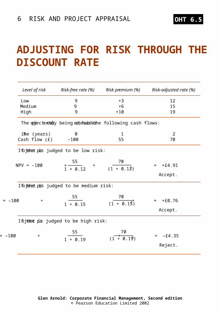
ADJUSTING FOR RISK THROUGH THE DISCOUNT RATE

Level of risk Risk-free rate (%) Risk premium (%) Risk-adjusted rate (%)

Low 9 +3 12Medium 9 +6 15High 9 +10 19

The project currently being considered has the following cash flows:

Time (years) 0 1 2Cash flow (£) –100 55 70

If the project is judged to be low risk:

55 70NPV = –100 + + = +£4.91

1 + 0.12 2

Accept.

If the project is judged to be medium risk:

55 70NPV = –100 + + = +£0.76

1 + 0.152

Accept.

If the project is judged to be high risk:

55 70NPV = –100 + + = –£4.35

1 + 0.192

Reject.

(1 + 0.12)

(1 + 0.15)

(1 + 0.19)



OHT 6.6

Adjusting for risk

Drawbacks of the risk-adjusted discount rate method:

• Risk classification is subjective• Difficulty in selecting risk premiums



OHT 6.7

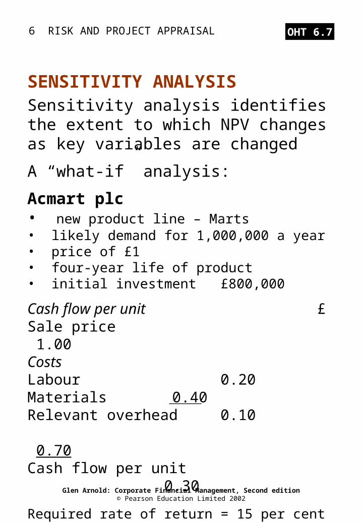
Sensitivity analysis identifies the extent to which NPV changes as key variables are changed

A “what-if” analysis:

Acmart plc• new product line – Marts• likely demand for 1,000,000 a year• price of £1• four-year life of product• initial investment £800,000

Cash flow per unit £Sale price 1.00CostsLabour 0.20Materials 0.40Relevant overhead 0.10

0.70Cash flow per unit 0.30

Required rate of return = 15 per cent

SENSITIVITY ANALYSIS



OHT 6.8

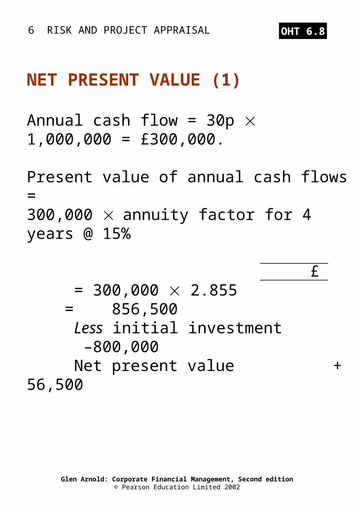
Annual cash flow = 30p 1,000,000 = £300,000.

Present value of annual cash flows = 300,000 annuity factor for 4 years @ 15%

£= 300,000 2.855 = 856,500Less initial investment –800,000Net present value + 56,500

NET PRESENT VALUE (1)



OHT 6.9

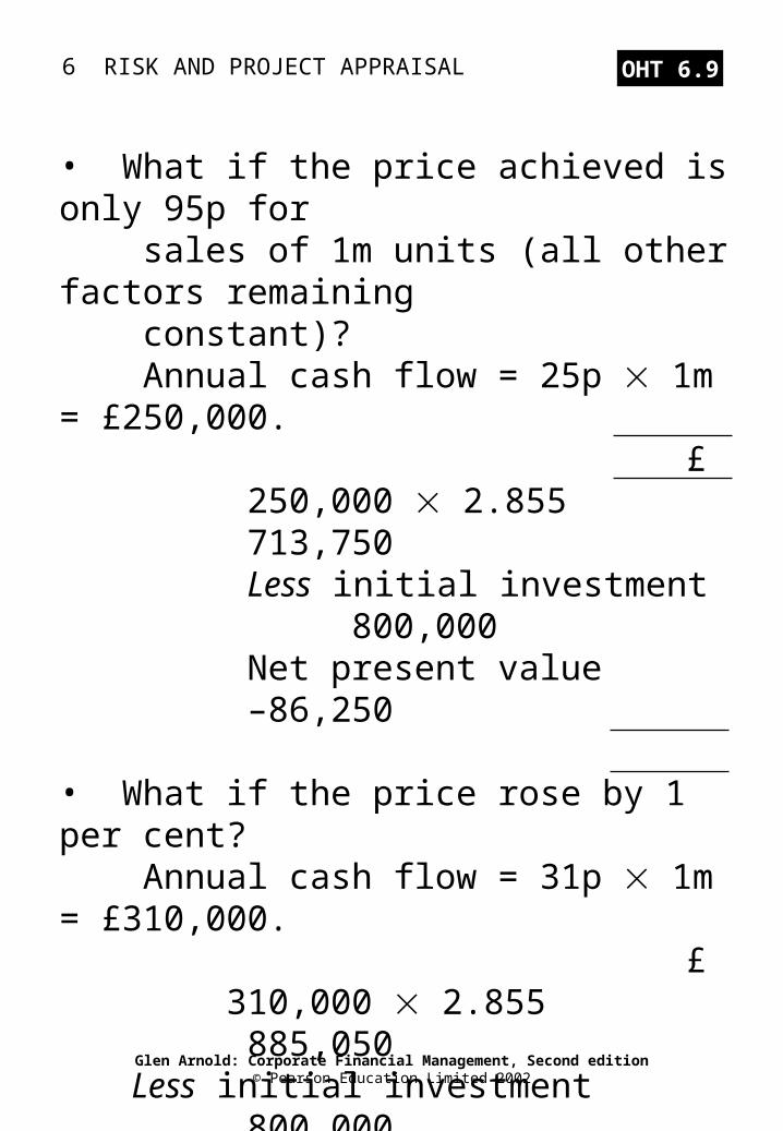
• What if the price achieved is only 95p for sales of 1m units (all other factors remaining constant)? Annual cash flow = 25p 1m = £250,000.

£ 250,000 2.855 713,750 Less initial investment 800,000 Net present value –86,250

• What if the price rose by 1 per cent? Annual cash flow = 31p 1m = £310,000.

£ 310,000 2.855 885,050 Less initial investment 800,000 Net present value +85,050



OHT 6.10

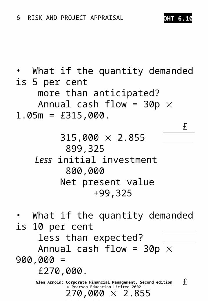
• What if the quantity demanded is 5 per cent more than anticipated? Annual cash flow = 30p 1.05m = £315,000.

£ 315,000 2.855 899,325 Less initial investment 800,000 Net present value +99,325

• What if the quantity demanded is 10 per cent less than expected? Annual cash flow = 30p 900,000 = £270,000.

£ 270,000 2.855 770,850 Less initial investment 800,000 Net present value –29,150



OHT 6.11

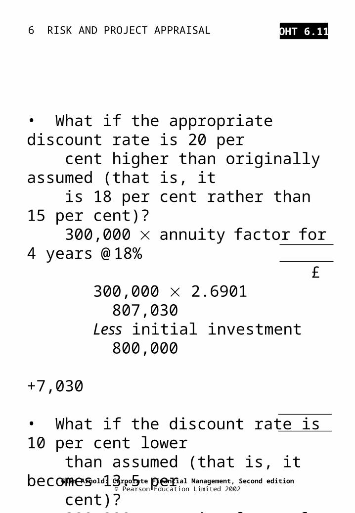
• What if the appropriate discount rate is 20 per cent higher than originally assumed (that is, it is 18 per cent rather than 15 per cent)? 300,000 annuity factor for 4 years @ 18%

£ 300,000 2.6901 807,030 Less initial investment 800,000

+7,030

• What if the discount rate is 10 per cent lower than assumed (that is, it becomes 13.5 per cent)? 300,000 annuity factor for 4 years @ 13.5%.

£ 300,000 2.9441 883,230 Less initial investment 800,000

+83,230



OHT 6.12

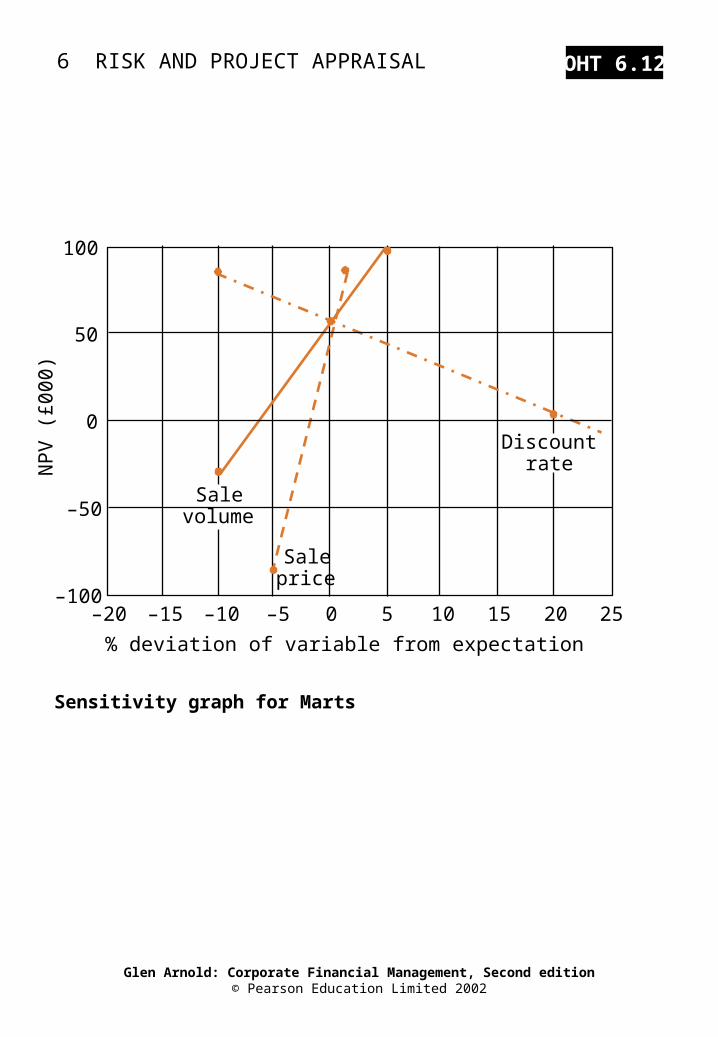
Sensitivity graph for Marts

–20–100

–15 –10 –5 0 5 10 15 20 25

–50

0

50

100

% deviation of variable from expectation

Saleprice

Salevolume

DiscountrateN

PV

(£0

00)



OHT 6.13

Break-even NPV calculations

Advantages of using sensitivity analysis:

• Information for decision making

• To direct search

• To make contingency plans

Drawbacks of sensitivity analysis:

• No formal assignment of probabilities

• Each variable is changed in isolation



OHT 6.14

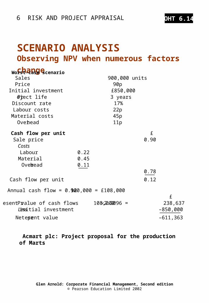
Acmart plc: Project proposal for the production of Marts

SCENARIO ANALYSIS Observing NPV when numerous factors change Worst-case scenarioSales 900,000 unitsPrice 90pInitial investment £850,000Project life 3 yearsDiscount rate 17%Labour costs 22pMaterial costs 45pOverhead 11p

Cash flow per unit £Sale price 0.90Costs

Labour 0.22Material 0.45Overhead 0.11

0.78

Cash flow per unit 0.12

Annual cash flow = 0.12 900,000 = £108,000£

Present value of cash flows 108,000 2.2096 = 238,637Less initial investment –850,000

Net present value –611,363



OHT 6.15

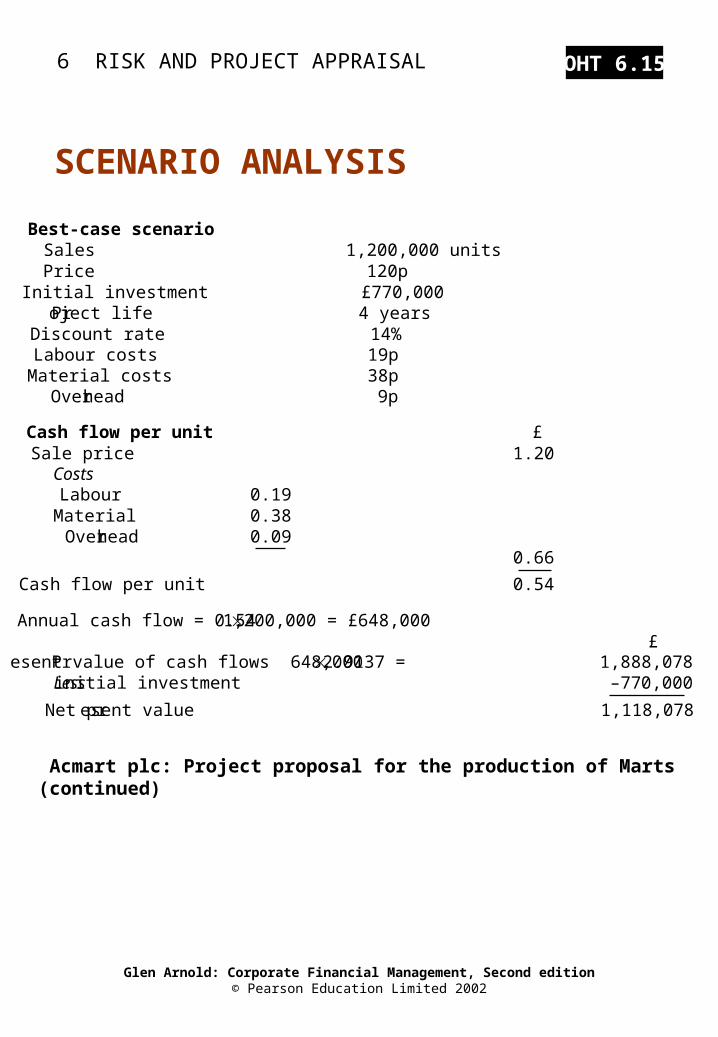
Acmart plc: Project proposal for the production of Marts (continued)

SCENARIO ANALYSIS

Best-case scenarioSales 1,200,000 unitsPrice 120pInitial investment £770,000Project life 4 yearsDiscount rate 14%Labour costs 19pMaterial costs 38pOverhead 9p

Cash flow per unit £Sale price 1.20Costs

Labour 0.19Material 0.38Overhead 0.09

0.66

Cash flow per unit 0.54

Annual cash flow = 0.54 1,200,000 = £648,000£

Present value of cash flows 648,000 2.9137 = 1,888,078Less initial investment –770,000

Net present value 1,118,078



OHT 6.16

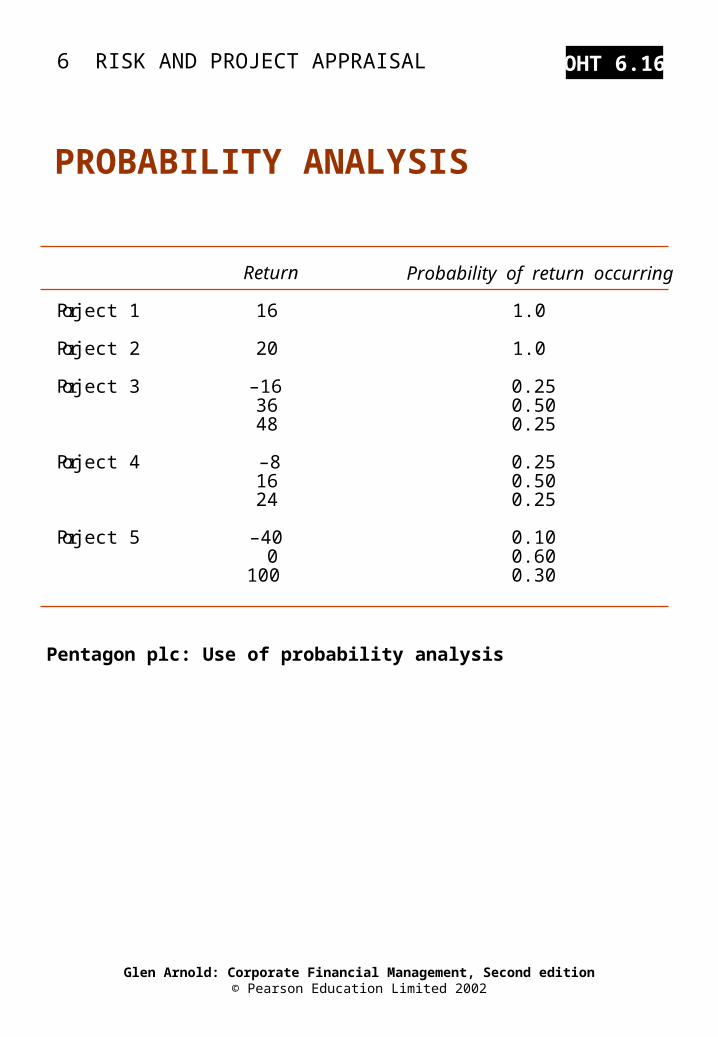
Pentagon plc: Use of probability analysis

PROBABILITY ANALYSIS

Return Probability of return occurring

Project 1 16 1.0

Project 2 20 1.0

Project 3 –16 0.2536 0.5048 0.25

Project 4 –8 0.2516 0.5024 0.25

Project 5 –40 0.100 0.60

100 0.30



OHT 6.17

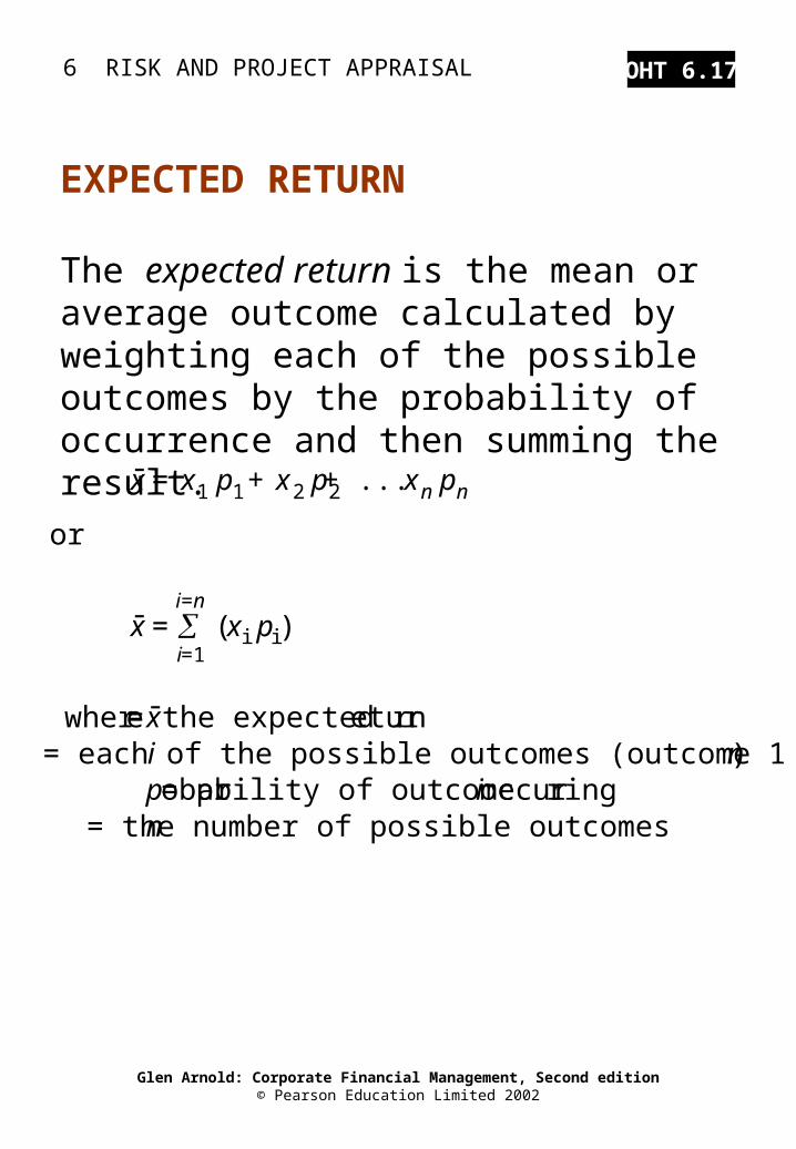
The expected return is the mean or average outcome calculated by weighting each of the possible outcomes by the probability of occurrence and then summing the result.

EXPECTED RETURN

x- = x1 p1 + x 2 p2 + ... x n pn

or

i=nx- = (x i pi)

i=1

where x- = the expected returni = each of the possible outcomes (outcome 1 to n) p = probability of outcome i occurringn = the number of possible outcomes



OHT 6.18

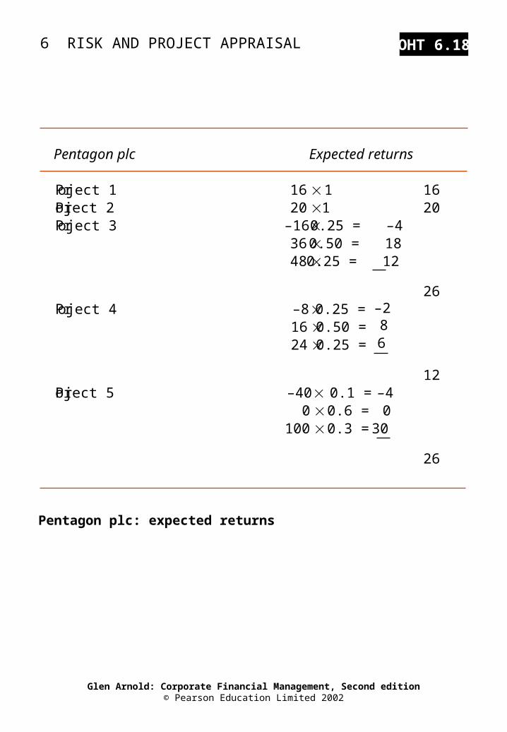
Pentagon plc: expected returns

Pentagon plc Expected returns

Project 1 16 1 16Project 2 20 1 20Project 3 –16 0.25 = –4

36 0.50 = 1848 0.25 = 12

26Project 4 –8 0.25 = –2

16 0.50 = 8

24 0.25 = 6

12Project 5 –40 0.1 = –4

0 0.6 = 0100 0.3 = 30

26



OHT 6.19

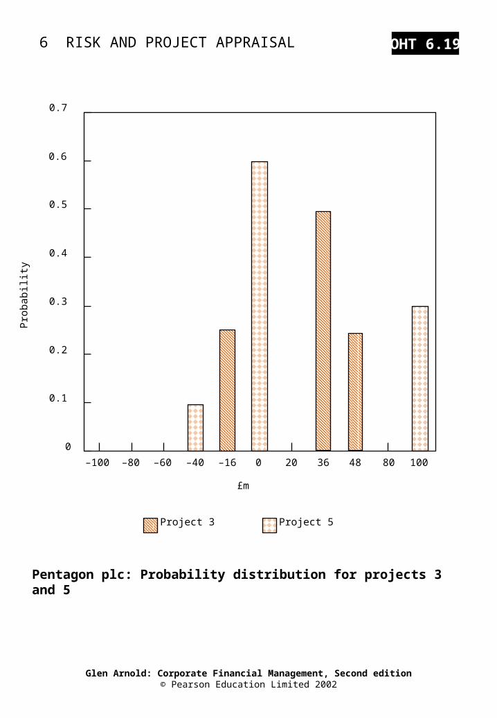
Pentagon plc: Probability distribution for projects 3 and 5

0

–100 –80 –60 –40 –16 0 20 36 48 80 100

0.1

0.2

0.3

0.4

0.5

0.6

0.7

£m

Project 3 Project 5

Pro

babi

lity



OHT 6.20

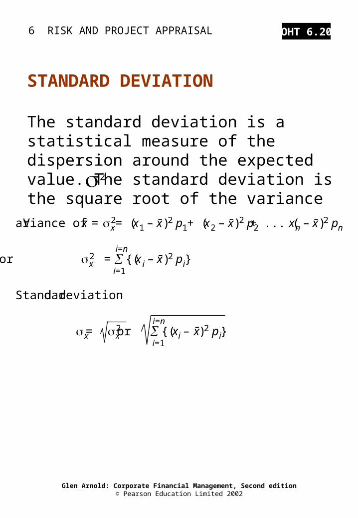
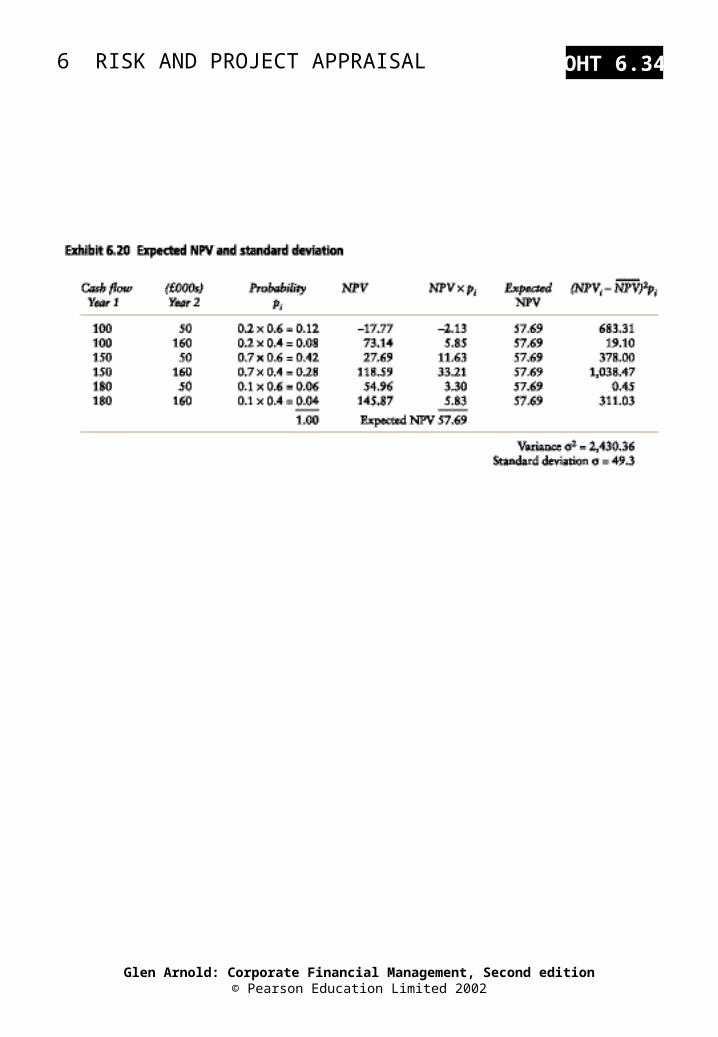
The standard deviation is a statistical measure of the dispersion around the expected value. The standard deviation is the square root of the variance

STANDARD DEVIATION

2

nVariance of x = x2 = (x1 – x- )2 p1 + (x2 – x- )2 p2 + ... (xn – x- )2 p

i=nor x

2 = {(x i – x- )2 pi}i=1

Standard deviation

i=n x = x

2 or {(xi – x- )2 pi}i=1



OHT 6.21

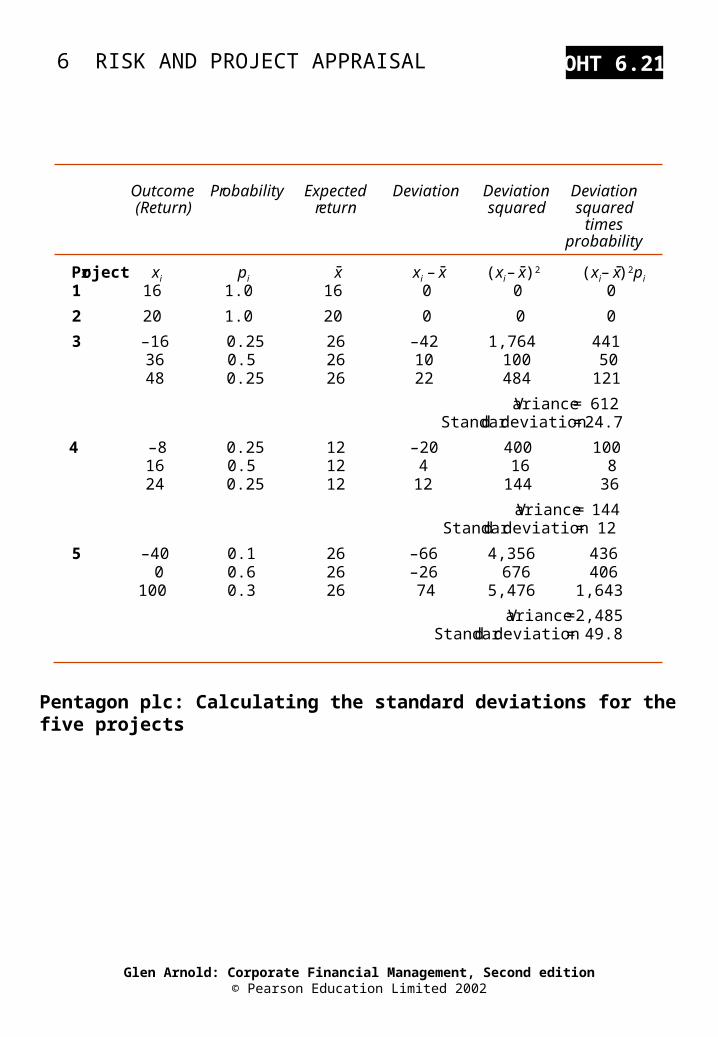
Pentagon plc: Calculating the standard deviations for the five projects

Outcome Probability Expected Deviation Deviation Deviation(Return) return squared squared

timesprobability

Project xi pi x- xi – x- (xi – x- )2 (xi – x- )2pi

1 16 1.0 16 0 0 0

2 20 1.0 20 0 0 0

3 –16 0.25 26 –42 1,764 44136 0.5 26 10 100 5048 0.25 26 22 484 121

Variance = 612Standard deviation = 24.7

4 –8 0.25 12 –20 400 10016 0.5 12 4 16 824 0.25 12 12 144 36

Variance = 144Standard deviation = 12

5 –40 0.1 26 –66 4,356 4360 0.6 26 –26 676 406

100 0.3 26 74 5,476 1,643

Variance = 2,485Standard deviation = 49.8



OHT 6.22

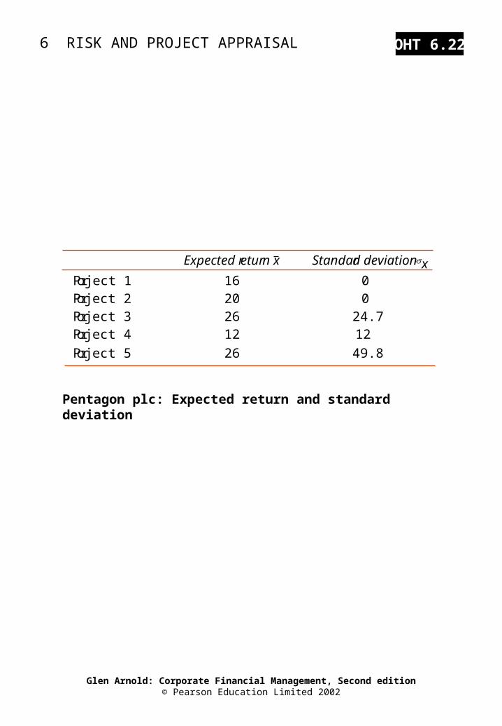
Pentagon plc: Expected return and standard deviation

Expected return x Standard deviation xProject 1 16 0Project 2 20 0Project 3 26 24.7Project 4 12 12

Project 5 26 49.8



OHT 6.23

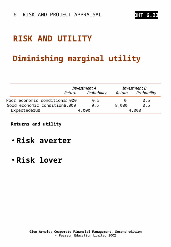
Returns and utility

• Risk averter

• Risk lover

RISK AND UTILITY

Diminishing marginal utility

Investment A Investment BReturn Probability Return Probability

Poor economic conditions 2,000 0.5 0 0.5Good economic conditions 6,000 0.5 8,000 0.5Expected return 4,000 4,000



OHT 6.24

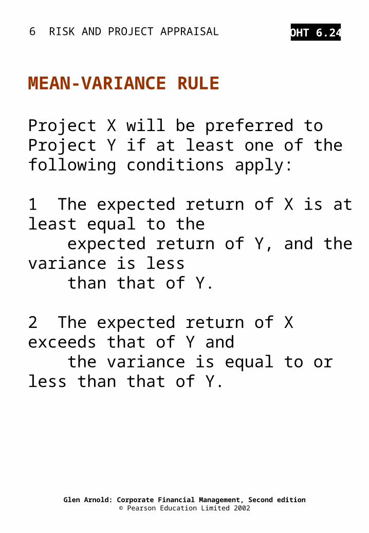
Project X will be preferred to Project Y if at least one of the following conditions apply:

1 The expected return of X is at least equal to the expected return of Y, and the variance is less than that of Y.

2 The expected return of X exceeds that of Y and the variance is equal to or less than that of Y.

MEAN-VARIANCE RULE



OHT 6.25

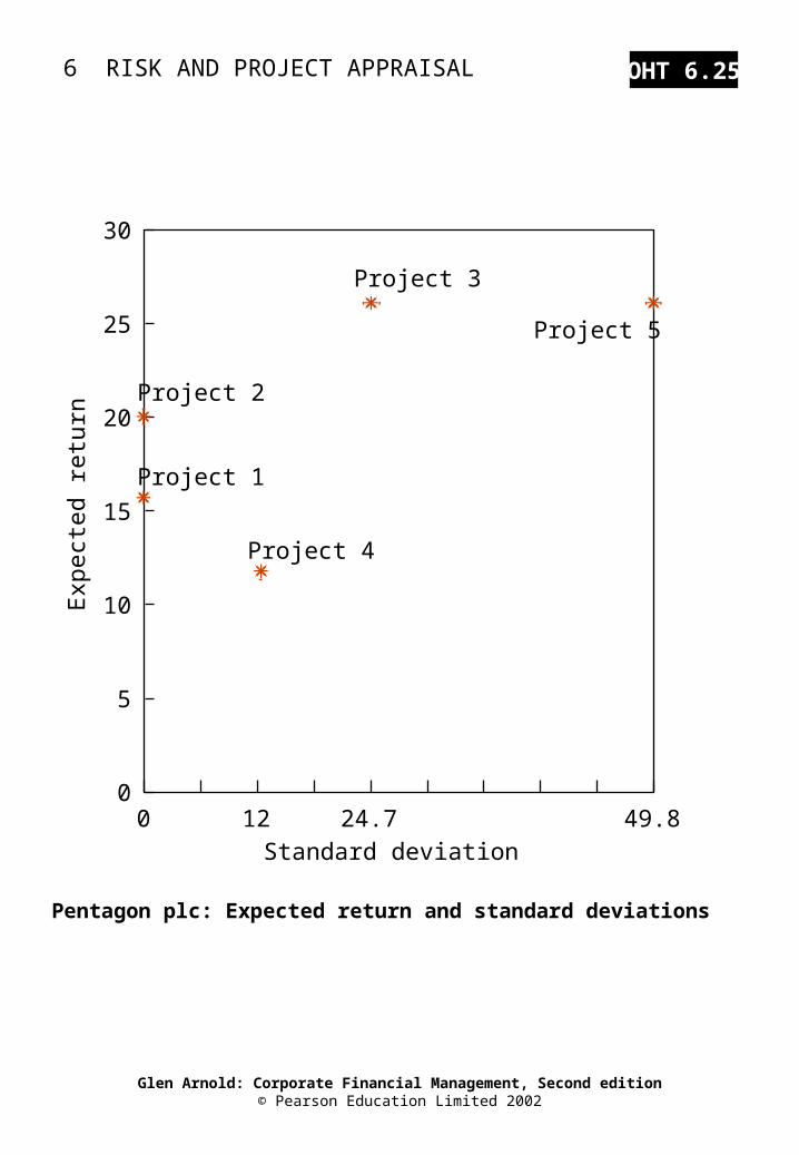
Pentagon plc: Expected return and standard deviations

00 12 24.7 49.8

5

10

15

20

25

30

Standard deviation

Project 1

Project 2

Project 4

Project 3

Project 5

Exp

ecte

d re

turn



OHT 6.26

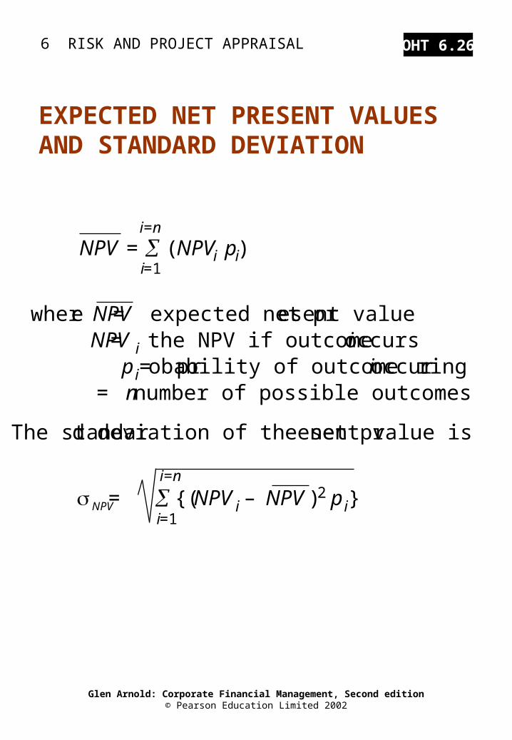
EXPECTED NET PRESENT VALUES AND STANDARD DEVIATION

i=n

NPV = (NPVi pi)i=1

where NPV = expected net present valueNPV i = the NPV if outcome i occurs

p i = probability of outcome i occurringn = number of possible outcomes

The standard deviation of the net present value is

i=n

NPV = {(NPV i – NPV )2 p i}i=1



OHT 6.27

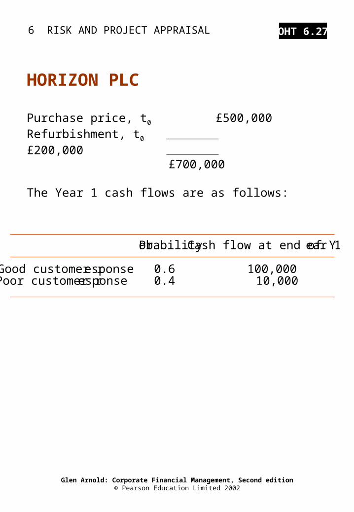
Purchase price, t0 £500,000Refurbishment, t0 £200,000

£700,000

The Year 1 cash flows are as follows:

HORIZON PLC

Probability Cash flow at end of Year 1

Good customer response 0.6 100,000Poor customer response 0.4 10,000



OHT 6.28

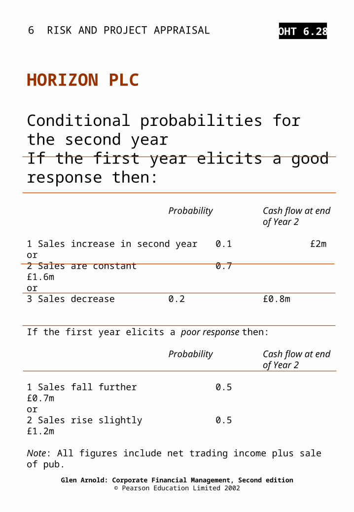
Conditional probabilities for the second yearIf the first year elicits a good response then:

Probability Cash flow at endof Year 2

1 Sales increase in second year 0.1 £2mor2 Sales are constant 0.7 £1.6mor3 Sales decrease 0.2 £0.8m

If the first year elicits a poor response then:

Probability Cash flow at endof Year 2

1 Sales fall further 0.5 £0.7mor2 Sales rise slightly 0.5 £1.2m

Note: All figures include net trading income plus sale of pub.

HORIZON PLC



OHT 6.29

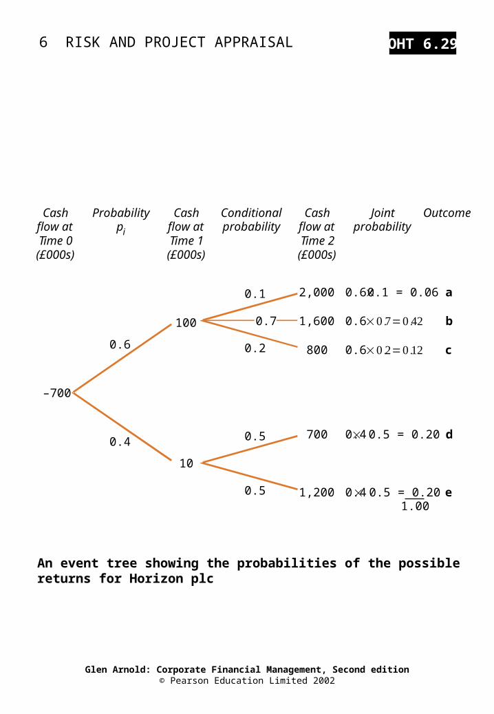
An event tree showing the probabilities of the possible returns for Horizon plc

Cashflow atTime 0(£000s)

–700

Probabilitypi


Conditionalprobability


Jointprobability

Outcome

100

10

2,000

800

1,600

700

1,200

0.1

0.2

0.5

0.5

0.7

0.6 0.1 = 0.06

0.6

0.6

0.4 0.5 = 0.20

0.4 0.5 = 0.201.00

0.6

0.4

a

c

b

d

e



OHT 6.30

(1.1)2

2,000

(1.1)2

800

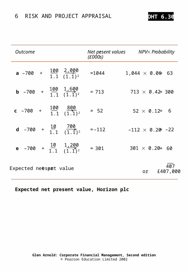
Expected net present value, Horizon plc

Outcome NPV ProbabilityNet present values(£000s)

100a –700 + + = 1044 1,044 0.06 = 631.1

100b –700 + + = 713 = 300

1.1

100c –700 + + = 52 = 6

1.1

10d –700 + + = –112 = –221.1

10e –700 + + = 301 = 601.1

Expected net present value 407or £407,000

(1.1)2

1,600

700(1.1)2

(1.1)2

1,200

713 0.42

52 0.12

–112 0.20

301 0.20



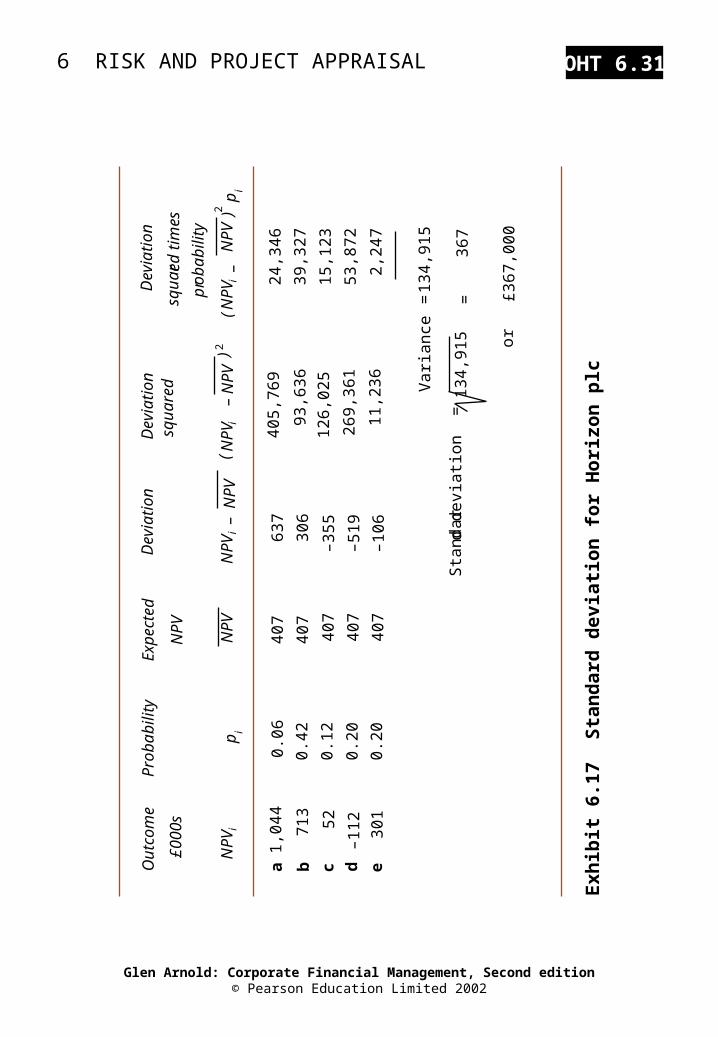
OHT 6.31

Exh

ibit

6.1

7 S

tan

dar

d d

evia

tion

for

Hor

izon

plc

Out

com

eP

roba

bili

tyE

xpec

ted

Dev

iati

onD

evia

tion

Dev

iati

on

£000

sN

PV

squa

red

squa

r ed

tim

es

prob

abil

ity

NP

V ip i

NP

VN

PV

i–

NP

V( N

PV i

–

NP

V)2

( NP

V i –

NP

V)2

pi

a1,

044

0.06

407

637

405,

769

24,3

46

b71

3 0.

42

407

306

93,6

3639

,327

c52

0.

12

407

–355

12

6,02

5 15

,123

d–1

12

0.20

40

7–5

19

269,

361

53,8

72

e30

1 0.

20

407

–106

11

,236

2,24

7

Var

ianc

e=

134,

915

Sta

ndar

d de

viat

ion

=13

4,91

5=

367

or£3

67,0

00



OHT 6.32

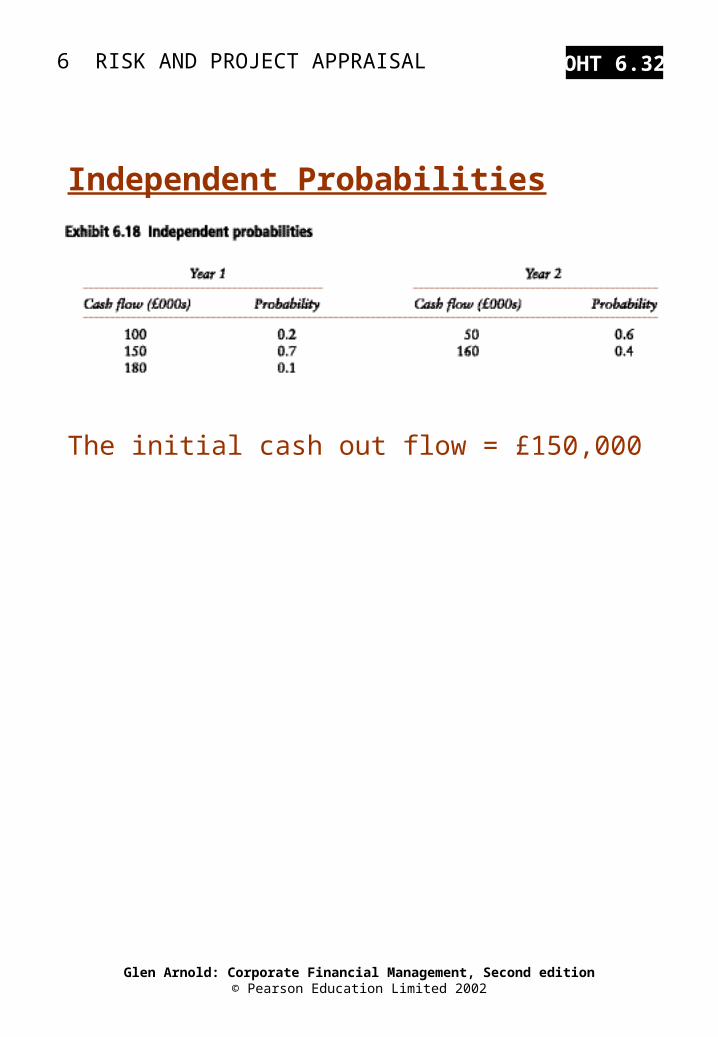
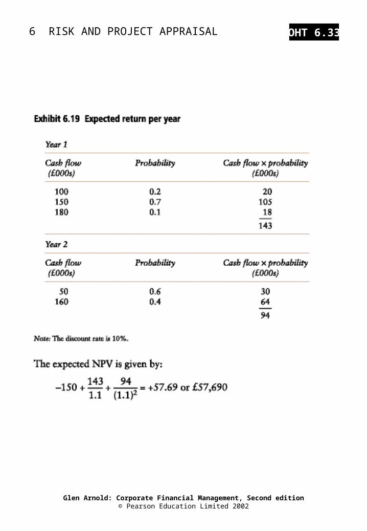
Independent Probabilities

The initial cash out flow = £150,000



OHT 6.33



OHT 6.34



OHT 6.35

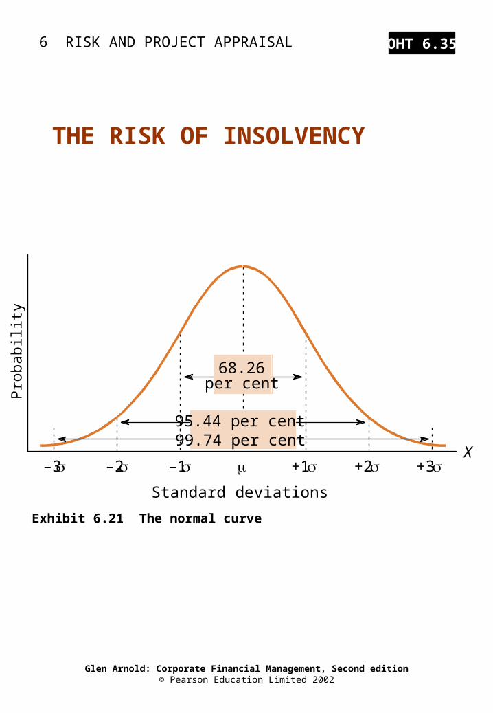
Exhibit 6.21 The normal curve

THE RISK OF INSOLVENCY

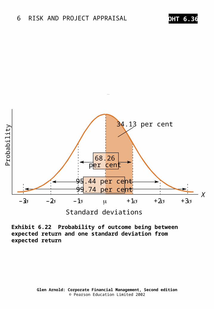
95.44 per cent99.74 per cent

68.26per cent

–3 –2 –1 +1 +2 +3

Standard deviations

X

Pro

babi

lity



OHT 6.36

Exhibit 6.22 Probability of outcome being between expected return and one standard deviation from expected return

–3 –2 –1 +1 +2 +3

Standard deviations

Probability

X

34.13 per cent

Pro

babi

lity

95.44 per cent99.74 per cent

68.26per cent



OHT 6.37

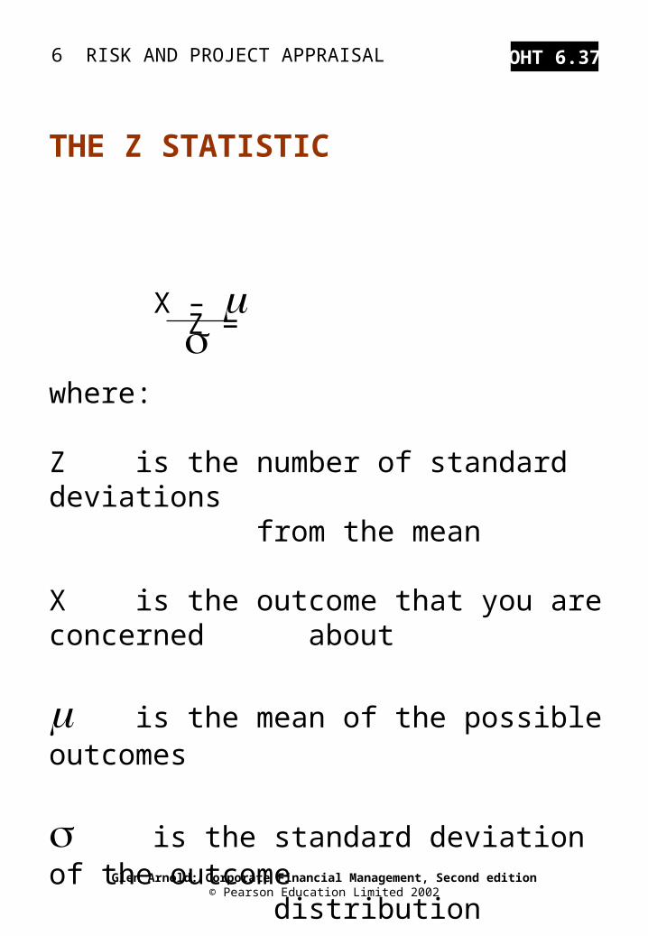
Z =

where:

Z is the number of standard deviations from the mean

X is the outcome that you are concerned about

is the mean of the possible outcomes

is the standard deviation of the outcome distribution

THE Z STATISTIC

X –



OHT 6.38

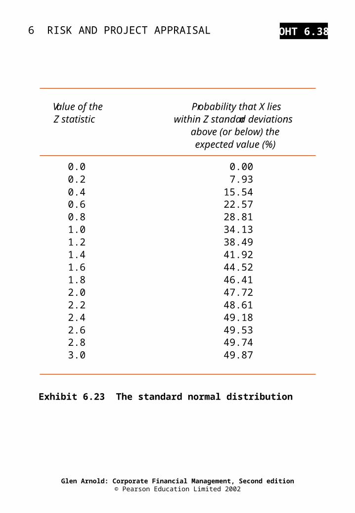
Exhibit 6.23 The standard normal distribution

Value of the Probability that X liesZ statistic within Z standard deviations

above (or below) the expected value (%)

0.0 0.000.2 7.930.4 15.540.6 22.570.8 28.811.0 34.131.2 38.491.4 41.921.6 44.521.8 46.412.0 47.722.2 48.612.4 49.182.6 49.532.8 49.743.0 49.87



OHT 6.39

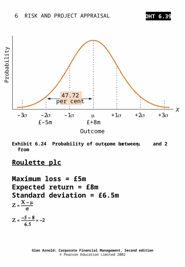
Exhibit 6.24 Probability of outcome between and 2 from

Roulette plc

Maximum loss = £5mExpected return = £8mStandard deviation = £6.5m

–3 –2 –1 +1 +2 +3

Outcome

Probability

X

47.72per cent

£–5m £+8m

Pro

babi

lity



OHT 6.40

• Too much faith can be placed in quantified subjective probabilities

• Too complicated for all managers to understand

• Projects may be viewed in isolation

PROBLEMS OF USING PROBABILITY ANALYSIS



OHT 6.41

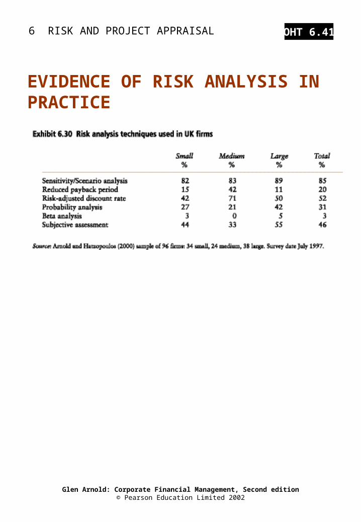
EVIDENCE OF RISK ANALYSIS IN PRACTICE

Documents

Adjust for risk by varying the discount rate Present a sensitivity graph and discuss