Embed Size (px)
Citation preview
THE JOURNAL OF FINANCE • VOL. LIX, NO. 6 • DECEMBER 2004
How to Discount Cashflows with Time-VaryingExpected Returns
ANDREW ANG and JUN LIU∗
ABSTRACT
While many studies document that the market risk premium is predictable and thatbetas are not constant, the dividend discount model ignores time-varying risk pre-miums and betas. We develop a model to consistently value cashflows with changingrisk-free rates, predictable risk premiums, and conditional betas in the context of aconditional CAPM. Practical valuation is accomplished with an analytic term struc-ture of discount rates, with different discount rates applied to expected cashflows atdifferent horizons. Using constant discount rates can produce large misvaluations,which, in portfolio data, are mostly driven at short horizons by market risk premiumsand at long horizons by time variation in risk-free rates and factor loadings.
TO DETERMINE AN APPROPRIATE DISCOUNT RATE for valuing cashflows, a manageris confronted by three major problems: the market risk premium must be esti-mated, an appropriate risk-free rate must be chosen, and the beta of the projector company must be determined. All three of these inputs into a standard CAPMare not constant. Furthermore, cashflows may covary with the risk premium,betas, or other predictive state variables. A standard Dividend Discount Model(DDM) cannot handle dynamic betas, risk premiums, or risk-free rates becausein this valuation method, future expected cashflows are valued at constantdiscount rates.
In this paper, we present an analytical methodology for valuing stochasticcashflows that are correlated with risk premiums, risk-free rates, and time-varying betas. All these effects are important. First, the market risk premiumis not constant. Fama and French (2002) argue that the risk premium moved toaround 2% at the turn of the century from 7% to 8% 20 years earlier.Jagannathan, McGratten, and Scherbina (2001) also argue that the marketex ante risk premium is time varying and fell during the late 1990s. Further-more, a large literature claims that a number of predictor variables, including
∗Ang is with Columbia University and NBER. Jun Liu is at UCLA. We would like tothank Michael Brandt, Michael Brennan, Bob Dittmar, John Graham, Bruce Grundy, RaviJagannathan, and seminar participants at the Australian Graduate School of Management,Columbia University, the Board of Governors of the Federal Reserve, and Melbourne BusinessSchool for comments. We also thank Geert Bekaert and Zhenyu Wang for helpful suggestions andespecially thank Yuhang Xing for constructing some of the data. We also thank Rick Green (theformer editor), and we are grateful to an anonymous referee for helpful comments that greatlyimproved the paper. The authors acknowledge funding from an INQUIRE UK grant. This paperrepresents the views of the authors and not of INQUIRE. All errors are our own.
2745

2746 The Journal of Finance
dividend yields (Campbell and Shiller (1988a, b)), risk-free rates (Fama andSchwert (1977)), term spreads (Campbell (1987)), default spreads (Keimand Stambaugh (1986)), and consumption–asset–labor deviations (Lettau andLudvigson (2001)), have forecasting power for market excess returns.
Second, the CAPM assumes that the riskless rate is the appropriate one-period, or instantaneous, riskless rate, which in practice is typically proxied bya 1-month or a 3-month T-bill return. However, it is highly unlikely that overthe long horizons of many corporate capital budgeting problems the risklessrate remains constant. Since the total expected return comprises both a risk-free rate and a risk premium, adjusted by a factor loading, time-varying risk-free rates imply that total expected returns also change through time. Notethat even an investor who believes that the expected market excess return isconstant, and a project’s beta is constant, still faces stochastic total expectedreturns as short rates move over time.
Finally, as companies grow, merge, or invest in new projects, their risk profileschange. It is quite feasible that a company’s beta changes even in short intervals,and it is very likely to change over 10- or 20-year horizons. There is substantialvariation in factor loadings even for portfolios of stocks, for example, industryportfolios (Fama and French (1997)) and portfolios sorted by size and book-to-market (Ferson and Harvey (1999)) ratio. The popularity of multifactor modelsfor computing unconditional expected returns (e.g., Fama and French (1993))may reflect time-varying betas and conditional market risk premiums in aconditional CAPM (see Jagannathan and Wang (1996)).
This paper presents, to our knowledge, the first analytic, tractable methodof discounting cashflows that embeds the effects of changing market risk pre-miums, risk-free rates, and time-varying betas. Previous practice adjusts theDDM by using different regimes of cashflow growth or expected returns (seeLee, Myers, and Swaminathan (1999) for a recent example). These adjustmentsare not made in an overall framework and so are subject to Fama’s (1996) cri-tique of ad hoc adjustments to cashflows with changing expected returns. Incontrast, our valuation is done in an internally consistent framework.
Our valuation framework significantly extends the current set of analyticpresent value models developed in the affine class (see, among others, Angand Liu (2001), Bakshi and Chen (2001), Bekaert and Grenadier (2001)). Ifa security’s beta is constant and the market risk premium is time varying,then the price of the security would fall into this affine framework. Similarly,the case of a time-varying beta and a constant market risk premium can alsobe handled by an affine model. However, unlike our setup, the extant class ofmodels cannot simultaneously model time variation in both beta and the marketrisk premium. This is because the expected return involves a product of twostochastic, predictable variables (beta multiplied by the market premium).
We derive our valuation formula under a very rich set of conditional ex-pected returns. Our functional form for time-varying expected returns neststhe specifications of the conditional CAPM developed by Harvey (1989), Fersonand Harvey (1991, 1993, 1999), Cochrane (1996), and Jagannathan and Wang

How to Discount Cashflows with Time-Varying Expected Returns 2747
(1996), among others. These studies use instrumental variables to model thetime variation of betas or market risk premiums. In our framework, shortrates also vary through time. The setup also incorporates correlation betweenstochastic cashflows, betas, and risk premiums.
To adapt our valuation framework to current practice in capital budgeting,we compute a term structure of discount rates applied to random cashflows.Practical cashflow valuation separates the problem into two steps: first, es-timate the expected future cashflows of a project or security, and then taketheir present value, usually by applying a constant discount rate. Instead ofapplying a constant discount rate, we compute a series of discount rates, orspot expected returns, which can be applied to a series of expected cashflows.The model incorporates the effects of changing market risk premiums, risk-freerates, and time-varying betas by specifying a different discount rate for eachdifferent maturity.
Brennan (1997) also considers the problem of discounting cashflows withtime-varying expected returns and proposes a term structure of discount rates.Our model significantly generalizes Brennan’s formulation. In his setup, thebeta of the security is constant and only the risk premium changes. Further-more, his discount rates can only be computed by simulation and were notapplied to valuing predictable cashflows. In contrast, our discount rates aretractable, analytic functions of a few state variables known at each point intime. We use this analytic form to attribute the mispricing effects of time-varying discount rates.
We illustrate a practical application of our theoretical framework by workingwith cashflows and expected returns of portfolios sorted by book-to-marketratios and industry portfolios. First, we compute the term structure of discountrates at the end of our sample, December 2000, for each portfolio. At this pointin time, the term structure of discount rates is upward sloping and much lowerthan a constant discount rate computed from the CAPM. Second, we computethe potential mispricing of ignoring the time variation of expected returns. Tofocus on the effects of time-varying discount rates, we compute the value of aperpetuity of an expected cashflow of $1 received each year, using the termstructure of discount rates from each portfolio. Ignoring time-varying expectedreturns can induce large potential misvaluations; mispricings of over 50% usinga traditional DDM are observed.
To determine the source of the mispricings, we use our model to decomposethe variance of the spot expected returns into variation due to each of theseparate components betas: risk-free rates and the risk premium. We find thatmost of the variation is driven by changes in beta and risk-free rates at longhorizons, while it is most important to take into account the variation of therisk premium at short horizons.
The rest of this paper is organized as follows. Section I presents a model forvaluing stochastic cashflows with time-varying expected returns. In Section II,we show how to compute the term structure of discount rates corresponding toour valuation model and derive variance decompositions for the discount rates.
2748 The Journal of Finance
We apply the model to data, which we describe in Section III. The empiricalresults are discussed in Section IV. Section V concludes.
I. Valuing Cashflows with Time-Varying Expected Returns
In this section, our contribution is to develop a closed-form methodology forcomputing spot discount rates in a system that allows for time-varying cashflowgrowth rates, betas, short rates, and market risk premiums. We begin with thestandard definition of a security’s expected return.
An asset pricing model specifies the expected return of a security, where thelog expected return µt is defined as1
exp(µt) = Et
[Pt+1 + Dt+1
Pt
], (1)
where Pt is the price and Dt is the cashflow of the security. If, in addition, thecashflow process Dt is also specified, then the price Pt of the security can bewritten as
Pt = Et
[ ∞∑s=1
(s−1∏k=0
exp(−µt+k)
)Dt+s
]. (2)
Equation (2) can be derived by iterating equation (1) and assuming transver-sality.
A traditional Gordon model formula assumes that the expected return isconstant, µt = µ, and the expected rate of cashflow growth is also constant:
Et[Dt exp(gt+1)] = Et[Dt+1] = Dt exp( g ).
In this case, the cashflow effects and the discounting effects can be separated:
Pt =∞∑
s=1
Et[Dt+s]exp(sµ)
. (3)
This reduces equation (2) to
Pt
Dt=
∞∑j=1
exp(−s · (µ − g )) = 1exp(µ − g ) − 1
,
which is the DDM formula, expressed with continuously compounded returnsand growth rates.
However, as many empirical and theoretical studies suggest, expected re-turns and cashflow growth rates are time varying and correlated. When thisis the case, the simple discounting formula (3) does not hold. In particular, theeffect of the cashflow growth rates cannot be separated from the effect of the
1 In equation (1), expected returns are continuously compounded to make the mathematicalexposition simpler.
How to Discount Cashflows with Time-Varying Expected Returns 2749
time-varying discount rates. We must then evaluate equation (2) directly. Inorder to take this expectation, we specify a rich class of conditional expectedreturns.
Consider a conditional log expected return µt specified by a conditional CAPM:
µt = α + rt + βtλt , (4)
where α is a constant, rt is a risk-free rate, βt is the time-varying beta, and λtis the time-varying market risk premium. In the class of conditional CAPMsconsidered by Harvey (1989), Shanken (1990), Ferson and Harvey (1991, 1993),and Cochrane (1996), among others, the time-varying beta or risk premium areparameterized by a set of instruments zt in a linear fashion. For example, theconditional risk premium can be predicted by zt:
λt ≡ Et[
ymt+1 − rt
] = b0 + b′1zt , (5)
where ymt+1 − rt is the log excess return on the market portfolio. Similarly, the
conditional beta can be predicted by zt and past betas:
Et[βt+1] = c0 + c′1zt + c2βt . (6)
The instrumental variables zt may be any variables that predict cashflows,betas, or aggregate returns. For example, Harvey (1989) specifies expected re-turns of securities to be a linear function of market returns, dividend yields,and interest rates. Jagannathan and Wang (1996) allow for conditional expectedmarket returns to be a function of labor and interest rates. Ferson and Harvey(1991, 1993) allow both time-varying betas and market risk premiums to belinearly predicted by factors such as inflation, interest rates, and GDP growth,while Ferson and Korajzyck (1995) allow time-varying betas in an APT model.In Cochrane (1996), betas can be considered to be a linear function of sev-eral instrumental variables, which also serve as the conditioning informationset.
To take the expectation (2), we need to know the evolution of the instrumentszt, the betas βt, and the cashflows of the security gt, where gt+1 = ln(Dt+1/Dt).Suppose we can summarize these variables by a K × 1 state-vector Xt, whereXt = (gtβtz′
t)′. The first and second elements of Xt are cashflow growth and
the beta of the asset, respectively, but this ordering is solely for convenience.Suppose that Xt follows a VAR(1):
X t = c + �X t−1 + �1/2εt , (7)
where εt ∼ IID N(0, I). The one-order lag specification of this process is notrestrictive, as additional lags may be added by rewriting the VAR into a com-panion form. Note that the instrumental variables zt can predict betas, as wellas market risk premiums, through the companion form � in (7).
The following proposition shows how to compute the price of the security (2)in closed form:
2750 The Journal of Finance
PROPOSITION 1: Let Xt = (gtβtz′t)
′, with dimensions K × 1, follow the process inequation (7). Suppose the log expected return (1) takes the form
µt = α + ξ ′X t + X ′t�X t , (8)
where α is a constant, ξ is a K × 1 vector and � is a symmetric K × K matrix.Then, assuming existence, the price of the security is given by
Pt = Et
[ ∞∑s=1
(s−1∏k=0
exp(−µt+k)
)Dt+s
],
Pt
Dt=
∞∑n=1
exp(a(n) + b(n)′X t + X ′t H(n)′X t),
(9)
where the coefficients a(n) is a scalar, b(n) is a K × 1 vector, and H(n) is aK × K symmetric matrix. The coefficients a(n), b(n), and H(n) are given by therecursions:
a(n + 1) = a(n) − α + (e1 + b(n))′c + c′H(n)c − 12 ln det(I − 2�H(n))
+ 12 (e1 + b(n) + 2H(n)c)′(�−1 − 2H(n))−1(e1 + b(n) + 2H(n)c),
b(n + 1) = −ξ + �′(e1 + b(n)) + 2�′H(n)c
+ 2�′H(n)(�−1 − 2H(n))−1(e1 + b(n) + 2H(n)c),
H(n + 1) = −� + �′H(n)� + 2�′H(n)(�−1 − 2H(n))−1 H(n)�,
(10)
where e1 represents a vector of zeros with a 1 in the first place and
a(1) = −α + e′1c + 1
2 e′1�e1,
b(1) = −ξ + �′e1,
H(1) = −�.
(11)
The general formulation of the expected return in equation (8) can be appliedto the following special cases:
1. First, the trivial case is that µt = µ is constant, so ξ = � = 0, α > 0, givingthe standard DDM in equation (3).
2. Second, equation (8) nests a conditional CAPM relation with time-varyingbetas and short rates by specifying zt = rt, the short rate, so Xt = (gtβtrt)′.The one-period expected return follows:
µt = α + rt + βt λ = α + (e3 + λe2)′X t , (12)
where λ is the constant market risk premium and ei represents a vectorof zeros with a 1 in the ith place. Hence, we can set ξ = (e3 + λe2) and� = 0.

How to Discount Cashflows with Time-Varying Expected Returns 2751
3. Third, if the market risk premium is predictable, but the security orproject’s beta is constant (βt = β), then we can specify Xt = (gtrtzt)′, wherezt are predictive instruments forecasting the market risk premium:
λt ≡ Et[
ymt+1 − rt
] = b0 + b′1zt .
The expected return then becomes
µt = α + rt + βλt = α + (e2 + βb1)′X t ,
so we can set ξ = (e2 + βb1) and � = 0.4. Finally, we can accommodate both time-varying betas and risk premiums.
If the market risk premium λt = b0 + b′1zt and Xt is given by our full speci-
fication Xt = (gtβtz′t)
′, then the conditional expected return can be writtenas
µt = α + rt + λtβt = α + rt + b0βt + βt(b′1zt). (13)
If rt is included in the instrument set zt, then equation (13) takes the formof equation (8) for appropriate choices of ξ and �. The quadratic term �
is now nonzero to reflect the interaction term of βt(b′1zt).
The quadratic Gaussian structure of the discount rate µt in equation (8)results from modeling the interaction of stochastic betas and stochastic riskpremiums. Quadratic Gaussian models have been used in the finance literaturein other applications. For example, Constantinides (1992) and Ahn, Dittmar,and Gallant (2002) develop quadratic Gaussian term structure models. Kimand Omberg (1996), Campbell and Viceira (1999), and Liu (1999), among others,apply quadratic Gaussian structures in portfolio allocation.
The pricing formula in equation (9) is analytic because the coefficients a(n),b(n), and H(n) are known functions and stay constant through time. Prices movebecause cashflow growth or state variables affecting expected returns change inXt. The class of affine present value models in Ang and Liu (2001), Bakshi andChen (2001), and Bekaert and Grenadier (2001) only have the scalar and linearrecursions a(n) and b(n). Our model has an additional recursion for a quadraticterm H(n). The extant class of present value models is unable to handle theinteraction between betas and risk premiums. Note that the quadratic H(n)term also affects the recursions of a(n) and b(n).2
In our analysis, we consider only a CAPM formulation with time-varyingbetas and time-varying market risk premiums, but Proposition 1 is generalenough to model time-varying betas for multiple factors, as well as time-varyingrisk premiums for multiple factors. This generalized setting would include lin-ear multifactor models, like the Fama and French (1993) three-factor model.In this case, Xt would now include time-varying betas with respect to each of
2 Alternative approaches are taken by Berk, Green, and Naik (1999), who use a dynamic optionsapproach, and Menzly, Santos, and Veronesi (2003), who price stocks in a habit economy by spec-ifying the fraction each asset contributes to total consumption. In contrast, we specify exogenouscashflows in a way that is easily adaptable to current valuation practice.

2752 The Journal of Finance
the factors, and the instrumental variables zt could predict each of the factorpremiums.
In Proposition 1, we assume that beta is an exogenous process and solveendogenously for the price of the security. Using the exogenously specified ex-pected returns and cashflows, we can construct return series for individualassets, and, if the number of shares outstanding of each asset is specified, wecan construct the return series of the market portfolio. We can compute thecovariance of an individual stock return and the aggregate market portfolio,and hence compute the implied beta of the stock from returns. Therefore, betais both an input to the model and an output of the model. The beta specified asan input into the VAR in equation (7) and the resulting beta from the impliedreturns from Proposition 1 are not necessarily the same. To see this, our modelassumes that the market return takes the following form:
ymt+1 − rt = λt(X t) + σm
t (X t)vmt+1, (14)
where λt is the same market risk premium in equation (4). The continuouslycompounded returns of security i implied by the prices from Proposition 1 satisfy
yit+1 − rt + 1
2
(σ i
t (X t))2 = βi
t
(ym
t+1 − rt) + σ i
t (X t)uit+1, (15)
where 12 (σ i
t (X t))2 is the Jensen’s term from working in continuously compoundedreturns, yi
t+1 − rt is the excess return for asset i, and σ it (Xt) is the idiosyncratic
volatility of asset i that depends on state variables.3
We obtain returns in equation (15) using the relation yt+1 = (1 + Pt+1/Dt+1)/(Pt/Dt) × exp(gt+1). Heteroskedasticity in returns arises from the nonlinearform of equation (9), even though the driving process for Xt in equation (7) ishomoskedastic. The beta β i
t specified in the VAR in equation (7) is not the sameas covt( yi
t+1, ymt+1)/(σm
t )2 in equation (15). If we also aggregate the returns ofindividual stocks by multiplying equation (15) by the market weights ωi of eachasset i, we do not obtain equation (14). This is because of the heteroskedasticJensen’s term 1
2 (σ it (X t))2 introduced by the stock valuation equation (9). How-
ever, we would expect the discrepancy to be small, because σ it (Xt)2 in (15) is
small.The model’s implied beta from returns can be made the same as the model’s
beta in the VAR in three ways. First, we can simply ignore the small Jensen’sterm in equation (15). Second, we can perform a Campbell and Shiller (1988b)log-linearization on the returns implied from Proposition 1, equation (9),and then rewrite equation (15) using log-linearized returns. Both of these
3 Equations (14) and (15) represent an arbitrage-free specification, since there is a strictly posi-tive pricing kernel mt+1 that supports these returns:
mt+1 = R−1t exp
(−1
2λ2
t
(σ mt )2
− λt
σ mt
vmt+1
),
where Rt is the gross risk-free rate Rt = exp(rt).

How to Discount Cashflows with Time-Varying Expected Returns 2753
approximations imply that an asset’s returns satisfy a conditional version of anAPT model, where ∑
i
ωiβit = 1 and
∑i
ωiσiui
t+1 = 0.
The second relation is the standard assumption of a factor or APT model. Thatis, as the number of assets becomes large, diversification causes idiosyncraticrisk to tend to zero.
Finally, we can change the model specification. Proposition 1 specifies thelog discount rate to be a quadratic Gaussian process. This ensures that thediscount rate is always positive. Instead, we could work in simple returns, fol-lowing the conditional CAPM specified by Ferson and Harvey (1993, 1999). Ifwe specify the simple discount rate to be a quadratic Gaussian process, thenequation (9) would become the sum of quadratic Gaussian multiplied by ex-ponential quadratic Gaussian terms, extending Ang and Liu (2001). Then, theimplied simple returns would satisfy equation (15) without the Jensen’s term,and the model’s beta used as an input into the VAR would be consistent withthe implied model beta from returns. However, this has the disadvantage of al-lowing negative discount rates and does not allow a term structure of discountrates for valuation to be easily computed (below).
A final comment is that, like any present value or term structure model,Proposition 1 has an implied stochastic singularity. By exogenously specifying abeta, risk premium, and risk-free rate, we specify an expected return. Combinedwith the cashflow process, this implies a market valuation that may not equalthe observed market price of the stock.
II. The Term Structure of Expected Returns
Current practical capital budgeting is a two-step procedure. First, managerscompute expected future cashflows Et[Dt+s] from projections, analysts’ fore-casts, or from extrapolation of historical data. A constant discount rate is com-puted, usually using the CAPM (see Graham and Harvey (2001)). The secondstep is to discount expected cashflows using this discount rate. The DDM allowsthis separation of cashflows and discount rates only because expected returnsare assumed to be constant.
Although Proposition 1 allows us to value stochastic cashflows with time-varying returns, it is hard to directly apply the proposition to practical situ-ations where the expected cashflow stream is separately estimated. To adaptcurrent practice to allow for time-varying expected returns, we maintain theseparation of the problem of estimating future cashflows and discounting thecashflows. However, we change the second part of the DDM valuation method.In particular, instead of a constant discount rate, we apply a series of dis-count rates to the expected future cashflows, where each expected future cash-flow is discounted at the discount rate appropriate to the maturity of thecashflow.
2754 The Journal of Finance
Et[Dt+1] Et[Dt+2] Et[Dt+3]
t t+1 t+2 t+3
µt( 1 )
µt( 2 )
µt( 3 )
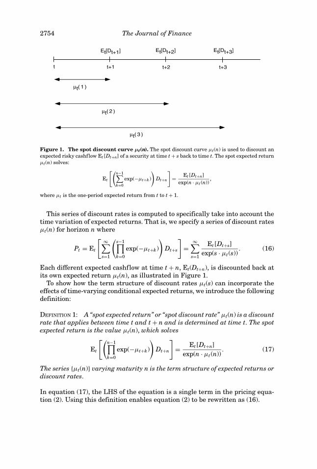
Figure 1. The spot discount curve µt(n). The spot discount curve µt(n) is used to discount anexpected risky cashflow Et [Dt+n] of a security at time t + s back to time t. The spot expected returnµt(n) solves:
Et
[(n−1∑k=0
exp(−µt+k)
)Dt+n
]= Et [Dt+n]
exp(n · µt (n)),
where µt is the one-period expected return from t to t + 1.
This series of discount rates is computed to specifically take into account thetime variation of expected returns. That is, we specify a series of discount ratesµt(n) for horizon n where
Pt = Et
[ ∞∑s=1
(s−1∏k=0
exp(−µt+k)
)Dt+s
]=
∞∑s=1
Et[Dt+s]exp(s · µt(s))
. (16)
Each different expected cashflow at time t + n, Et(Dt+n), is discounted back atits own expected return µt(n), as illustrated in Figure 1.
To show how the term structure of discount rates µt(s) can incorporate theeffects of time-varying conditional expected returns, we introduce the followingdefinition:
DEFINITION 1: A “spot expected return” or “spot discount rate” µt(n) is a discountrate that applies between time t and t + n and is determined at time t. The spotexpected return is the value µt(n), which solves
Et
[(n−1∏k=0
exp(−µt+k)
)Dt+n
]= Et[Dt+n]
exp(n · µt(n)). (17)
The series {µt(n)} varying maturity n is the term structure of expected returns ordiscount rates.
In equation (17), the LHS of the equation is a single term in the pricing equa-tion (2). Using this definition enables equation (2) to be rewritten as (16).
How to Discount Cashflows with Time-Varying Expected Returns 2755
The definition in equation (17) is a generalization of the term structure ofdiscount rates in Brennan (1997). Brennan restricts the time variation in ex-pected returns to come only from risk-free rates and market risk premiums,but ignores other sources of predictability (like time varying betas and cash-flows). The spot expected returns µt(n) depend on the information set at timet, and, as time progresses, the term structure of discount rates changes. Notethat the one-period spot expected return µt(1) is just the one-period expectedreturn applying between time t and t + 1, µt(1) ≡ µt.
To compute the spot expected returns µt(s), we use the following proposition:
PROPOSITION 2: Let Xt = (gtβtz′t)
′ follow the process in equation (7) and the one-period expected return µt follow equation (8). Then, assuming existence, the spotexpected return µt(n) is given by
µt(n) = A(n) + B(n)′X t + X ′tG(n)X t , (18)
where A(n) is a scalar, B(n) is a K × 1 vector, and G(n) is a K × K symmet-ric matrix. In the coefficients A(n) = (a(n) − a(n))/n, B(n) = (b(n) − b(n))/n, andG(n) = −H(n)/n, a(n), b(n) and H(n) are given by equation (10) in Proposition 1.The coefficients a(n) and b(n) are given by the recursions:
a(n + 1) = a(n) + e′1c + b(n)′c + 1
2 (e1 + b(n))′�(e1 + b(n))
b(n + 1) = �′(e1 + b(n)), (19)
where e1 represents a vector of zeros with a 1 in the first place and
a(1) = e′1c + 1
2 e′1�e1
b(1) = �′e1. (20)
Note that µt(n) is a quadratic function of Xt, the information set at time t.This is because the price of the security or asset is a function of exponentialquadratic terms of Xt in equation (9). As Xt changes through time, so do the spotexpected returns. This reflects the conditional nature of the expected returns,which depend on the state of the economy summarized by Xt. Like the termstructure of interest rates, the term structure of discount rates can take avariety of shapes, including upward sloping, downward sloping, humped andinverted shapes.
Besides being easily applied in practical situations, there are several reasonswhy our model’s formulation of spot expected returns is useful in the context ofvaluing cashflows. First, we compute the term structure of expected returns byspecifying models of the conditional expected return from a rich class of condi-tional CAPMs, used by many previous empirical studies. We can estimate thediscount curve for individual firms by looking at discount curves for industriesor for other groups of firms with similar characteristics (e.g., stocks with highor low book-to-market ratios).
Second, direct examination of the discount rate curve gives us a quick guideto potential mispricings between taking or not taking into account time-varying
2756 The Journal of Finance
expected returns. The greater the magnitude of the difference between the dis-count rates µt(n) and a constant discount rate µ, the greater the misvaluation.This difference is exacerbated at early maturities, where the time value ofmoney is large. Since the expected cashflows are the same in the numerator ofeach expression in equations (3) and (16), by looking at the difference betweenthe discount curve {µt(n)} and the constant expected return µ used in the stan-dard DDM, we can compare a valuation that takes into account the effects ofchanging expected returns to a valuation that ignores them.
Third, it may be no surprise that accounting for time-varying expected re-turns can lead to different prices from using a constant discount rate from anunconditional CAPM. What is economically more important is quantifying theeffects of time-varying expected returns by looking at their underlying sourcesof variation. Our analytic term structure of discount rates in Proposition 2allows us to attribute the effect of time-varying expected returns into theirdifferent components. For example, are time-varying risk-free rates the mostimportant source of variation of conditional expected returns, or is it more im-portant to account for time variation in the risk premium?
Finally, the discount curve is analogous to the term structure of zero-couponrates. In fixed income, cashflows are known, and the zero-coupon rates rep-resent the present value of $1 to be received at different maturities in thefuture. In equities, cashflows are stochastic (and are correlated with the time-varying expected return), and µt(n) represents the expected, rather than cer-tain, return of receiving future cashflows in the future at time t + n. In fixed-income markets, zero-coupon yields are observable, while in equity markets thespot discount rates are not observable. However, potentially one can obtain theterm structure of expected returns from observing the prices of stock futurescontracts of different maturities. For example, if a series of derivative securi-ties were available, with each derivative security representing the claim on astock’s dividend, payable only in each separate future period, the prices of thesederivative securities would represent the spot discount curve. Given the lack ofsuitable traded derivatives, particularly on portfolios, we directly estimate thediscount curves.
If a conditional CAPM is correctly specified, the constant α in equations (4) or(8) should be zero. Since the subject of this paper is to illustrate how to discountcashflows with time-varying expected returns, rather than correctly specifyingan appropriate conditional CAPM, in our empirical calibration, we include anα in the stock’s conditional expected return. Proposition 2 does not require theconditional CAPM to be exactly true. Hence, we include a constant to captureany potential misspecifications from a true conditional CAPM.
In addition to conducting a valuation incorporating all the time-varying risk-free, risk premium, and beta components, we also compute discount curvesrelative to two more special cases. First, if an investor correctly takes intoaccount the time-varying market risk premium, but ignores the time-varyingbeta, this also results in a misvaluation. We can measure this valuation byestimating a system Xt = (gtrtzt)′ that omits the time-varying beta and by usinga constant beta in the expected return µt = α + rt + βλt . The constant beta can

How to Discount Cashflows with Time-Varying Expected Returns 2757
be estimated using an unconditional CAPM. Second, an investor can correctlymeasure the time-varying beta, but ignore the predictability in the marketrisk premium. In this second system, the investor uses an expected returnµt = α + rt + βt λ, where λ is the unconditional mean of the market log excessreturn.
A. The Time Variation in Discount Rates
To investigate the source of the time variation in discount rates, we can com-pute the variance of the discount rate var(µt(n)), using the following corollary:
COROLLARY 1: The variance of the discount rate var(µt(n)) is given by
var(µt(n)) = B(n)′�X B(n) + 2tr((�X G(n))2), (21)
where �X is the unconditional covariance matrix of Xt, given by �X =devec((I − � ⊗ �)−1vec(�)).
It is possible to perform an approximate variance decomposition on (22), givenby the following corollary:4
COROLLARY 2: The variance of µt(n) can be approximated by
var(µt(n)) = (B(n) + 2G(n)X )′�X (B(n) + 2G(n)X ), (22)
ignoring the quadratic term in equation (21), where X = (I − �)−1c is the un-conditional mean of Xt.
We can use equation (22) to attribute the variation of µt(n) to variation of eachof the individual state variables in Xt. However, some of the sources of variationwe want to examine are transformations of Xt, rather than Xt itself. For example,a variance decomposition with respect to cashflows (gt) or betas (βt) can becomputed using equation (22) because gt and βt are contained in Xt. However,a direct application of equation (22) does not allow us to attribute the variationof µt(n) to sources of uncertainty driving the time variation in the market riskpremium λt, since λt is not included in Xt, but is a linear transformation of Xt. Toaccommodate variance decompositions of linear transformations of Xt, we canrewrite equation (22) using the mapping Zt = L−1(Xt − l) for L a K × K matrixand l a K × 1 vector:
var(µt(n)) = (B(n) + 2G(n)X )′L�Z L′(B(n) + 2G(n)X ), (23)
where �Z = L−1�X (L′)−1.Orthogonal variance decompositions can be computed using a Cholesky, or
similar, orthogonalizing transformation for �X or �Z. However, in our work,
4 The variance from the higher-order terms are extremely small, for our empirical values.

2758 The Journal of Finance
our variance decompositions do not sum to 1. For a single variable, we countall the contributions in the variance of that variable, together with all the co-variances with each of the other variables. Hence, our variance decompositionsdouble count the covariances, but are not subject to an arbitrary orthogonaliz-ing transformation.
III. Empirical Specification and Data
The model presented in Section II is very general, only needing cashflowsand betas to be included in a vector of state variables Xt. To illustrate theimplementation of the methodology, we specify the vector Xt that we use inour empirical application in Section A. Section B describes the data and thecalibration.
A. Empirical Specification
We specify Xt as Xt = (gtβt�potrtcaytπt)′, where gt is cashflow growth, βt isthe time-varying beta, �pot is the change in the payout ratio, rt is the nomi-nal short rate, cayt is Lettau and Ludvigson’s (2001) deviation from trend ofconsumption–asset–labor fluctuations, and πt is ex post inflation. We motivatethe inclusion of these variables as follows.
First, to predict the risk premium, we use nominal short rates rt and cayt. Tobe specific, we parameterize the market risk premium as
λt = b0 + brrt + bcaycayt . (24)
While many studies use dividend yields to predict market excess returns (seeCampbell and Shiller (1988a)), we choose not to use dividend yields becausethis predictive relation has grown very weak during the 1990s (see Ang andBekaert (2002), Goyal and Welch (2003)). In contrast, Ang and Bekaert (2002)and Campbell and Yogo (2002) find that the nominal short rate has strongpredictive power, at high frequencies, for excess aggregate returns. Lettau andLudvigson (2001) demonstrate that cayt is a significant forecaster of excess re-turns, at a quarterly frequency, both in-sample and out-of-sample. Both of thesepredictive instruments have stronger forecasting ability than the dividend yieldfor aggregate excess returns.
Second, to help forecast dividend cashflows gt, we use the change in thepayout ratio, which can be considered to be a measure of earnings growth inXt. Vuolteenaho (2002) shows that variation in firm-level earnings growth ac-counts for a large fraction of the variation of firm-level stock returns. However,earnings growth is difficult to compute for stock portfolios with high turnover.Instead, we use the change in the payout ratio, the ratio of dividends to earnings.This is equivalent to including earnings growth, since the change in the pay-out ratio, together with gt, contains equivalent information. To show this, if we

How to Discount Cashflows with Time-Varying Expected Returns 2759
denote earnings at time t as Earnt, then gross earnings growth Earnt/Earnt−1can be expressed as
Earnt
Earnt−1=
(1/pot
1/pot−1
)exp(gt),
where pot = Dt/Earnt represents the payout ratio.Finally, since movements in nominal short rates must be due either to move-
ments in real rates or inflation, we also include the ex post inflation rate πt inXt. This has the advantage of allowing us to separately examine the effects ofthe nominal short rate or the real interest rate.
To map the notation of Propositions 1 and 2 into this setup, we can specifythe formulation of the one-period expected return in equation (8) as follows:
µt = α + rt + λtβt
= α + e′4 X t + (b0 + brrt + bcaycayt)βt
= α + ξ ′X t + X ′t�X t , (25)
where ξ = (e4 + b0e2) and � is given by
� =
0 0 0 0 0 0
0 0 0 br/2 bcay/2 0
0 0 0 0 0 0
0 br/2 0 0 0 0
0 bcay/2 0 0 0 0
.
By applying Corollary 2, we can attribute the variation of µt(n) to lineartransformations of Xt. For example, to compute the variance decompositionof µt(n) to the risk premium λt, we can transform Xt = (gtβt�potrtcaytπt)′ toZt = (gtβt�potrtλtπt)′ using the mapping
X t = l + LZt ,
where l is a constant vector and L is a 6 × 6 matrix given by
L =
1 0 0 0 0 0
0 1 0 0 0 0
0 0 1 0 0 0
0 0 0 1 0 0
0 0 0 − brbcay
1bcay
− brbcay
0 0 0 0 0 1
.

2760 The Journal of Finance
B. Data Description and Estimation
To illustrate the effect of time-varying expected returns on valuation, wework with 10 book-to-market sorted portfolios and the Fama and French (1997)definitions of industry portfolios.5 We focus on these portfolios because of thewell-known value effect and because industry portfolios have varying exposureto various economic factors (see Ferson and Harvey (1991)). For the book-to-market portfolios, we focus on the deciles 1, 6, and 10, which we label “growth,”“neutral,” and “value,” respectively. We use data from July 1965 to December2000 for the book-to-market decile portfolios and from January 1964 to Decem-ber 2000 for the industry portfolios. All portfolios are value-weighted.
To estimate dividend cashflow growth rates of the portfolios, we computemonthly dividends as the difference between the portfolio value-weighted re-turns with dividends and capital gains, and the value-weighted returns exclud-ing dividends:
Pt+1/12 + Dt+1/12
Pt− Pt+1/12
Pt= Dt+1/12
Pt,
where the frequency 1/12 refers to monthly data. The bar superscript in thevariable Dt+1/12 denotes a monthly, as opposed to annual, dividend. To computeannual dividend growth, we sum up the dividends over the past 12 months, asis standard practice to remove seasonality (see Hodrick (1992)):
Dt =11∑
i=0
Dt−i/12.
Growth rates of cashflows are constructed taking logs gt = log(Dt/Dt−1). Thesecashflow growth rates represent annual increases of cashflows but are mea-sured at a monthly frequency.
To estimate time-varying betas on each portfolio, we employ the followingstandard procedure, dating back to at least Fama and MacBeth (1973). We runrolling 60-month regressions of the excess total return of the portfolio on aconstant and the excess market risk return:
yτ/12 − r(τ−1)/12 = αt + βt(
ymτ/12 − r(τ−1)/12
) + uτ , (26)
where all returns are continuously compounded, yτ/12 is the portfolio’s log totalreturn over month τ , r(τ−1)/12 is the continuously compounded 1-month risk-freerate (the 1-month T-bill rate) from (τ − 1)/12 to τ/12, and ym
τ/12 is the market’slog total return over month τ . The regression is run at a monthly frequencyfrom τ = t − 60/12 to τ = t. The time series of the estimated linear coefficientsin the regression (26) is the observable time series of the portfolio betas βt. Wecompute an α in equation (4) so that the average portfolio excess return in thedata is matched by this series of betas.
5 We exclude the industry portfolios Health, Miscellaneous, and Utilities because of missingdata.

How to Discount Cashflows with Time-Varying Expected Returns 2761
While this estimation procedure is standard and has been used by severalauthors to document time-varying betas, including recently Fama and French(1997), it is not the optimal method to estimate betas. If the VAR is correctlyspecified, then we should be able to infer the true, unobservable betas from thedata of realized returns, as well as the other observable variables in Xt, in amore efficient fashion. For example, Adrian and Franzoni (2002) use a Kalmanfilter to estimate time-varying betas, while Ang and Chen (2002) and Jostovaand Philipov (2002) employ a Gibbs sampler. However, these estimations arecomplex, and it is not the aim of this paper to use sophisticated econometricmethods to estimate betas. Rather, we focus on discounting cashflows undertime-varying betas, using a simple, standard procedure for estimating betas asan illustration.
To predict the market risk premium, we estimate the coefficients in the re-gression implied from equation (24):
ymt+1 − rt = b0 + brrt + bcaycayt + εt+1, (27)
where ymt+1 − rt is an annual market excess return, using a 1-year ZCB risk-free
rate. To form annual monthly returns, we first compute monthly log total re-turns on the market portfolio from month t/12 to (t + 1)/12 and then aggregateover 12 months to form annual log returns:
ymt+1 =
12∑i=1
ymt+i/12.
We use the monthly data in Lettau and Ludvigson (2002) to construct a seriesof cayt, which uses data only up to time t to estimate a cointegrating vector toestimate the consumption–wealth–labor deviation from trend at time t. Thisavoids any look-ahead bias in the construction of cayt (see Brennan and Xia(2002), and Hahn and Lee (2002)). All returns are continuously compounded,and the regression is run at a monthly frequency, but with an annual horizon.
We estimate our VAR in equation (7) and the predictability regression of ag-gregate excess returns in equation (27) at an annual horizon. That is, t to t + 1represents 1 year. Hence, we use 1-year ZCB risk-free rates rt, year-on-year logCPI inflation πt, and an annual change in the payout ratio, �pot, in the VAR.We define the payout ratio of year t to be the ratio of the sum of annual div-idends to summed annual earnings per share, excluding extraordinary items,of the companies in the portfolio. To compute this, we use the COMPUSTATannual file, and extract dividends and earnings of companies in the portfolio inDecember of year t. We exclude any companies with negative earnings.
To gain efficiency in estimating the VAR and the predictability regression,we use monthly data. Since we have annual horizons but monthly data, theresiduals from each regression in the VAR and in the predictability regressionhave an MA(11) form induced by the use of over-lapping observations. While allparameter estimates are consistent even with the overlap, the standard errorsof the parameters are affected by the MA(11) terms. To account for this, wereport standard errors computed using 12 Newey–West (1987) lags.
2762 The Journal of Finance
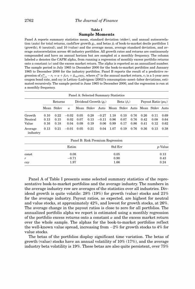
Table ISample Moments
Panel A reports summary statistics mean, standard deviation (stdev), and annual autocorrela-tion (auto) for total returns, cashflow growth gt, and betas βt of book-to-market decile portfolios 1(growth), 6 (neutral), and 10 (value) and the average mean, average standard deviation, and av-erage autocorrelation across 46 industry portfolios. All growth rates and returns are continuouslycompounded and have an annual horizon but are sampled at a monthly frequency. The columnlabeled α denotes the CAPM alpha, from running a regression of monthly excess portfolio returnsonto a constant (α) and the excess market return. The alpha is reported as an annualized number.The sample period is July 1965 to December 2000 for the book-to-market portfolios and January1965 to December 2000 for the industry portfolios. Panel B reports the result of a predictive re-gression of ym
t+1 − rt = α + βrrt + βcaycayt, where ymt is the annual market return, rt is a 1-year zero
coupon bond rate, and cay is Lettau–Ludvigson (2002)’s consumption–asset–labor deviations, esti-mated recursively. The sample period is June 1965 to December 2000, and the regression is run ata monthly frequency.
Panel A: Selected Summary Statistics
Returns Dividend Growth (gt) Beta (βt) Payout Ratio (pot)
Mean Stdev α Mean Stdev Auto Mean Stdev Auto Mean Stdev Auto
Growth 0.10 0.22 −0.02 0.05 0.28 −0.27 1.18 0.10 0.76 0.26 0.11 0.69Neutral 0.13 0.15 0.02 0.07 0.13 −0.11 0.96 0.07 0.76 0.42 0.08 0.64Value 0.16 0.18 0.04 0.09 0.19 0.06 0.99 0.17 0.86 0.41 0.12 0.62
Average 0.13 0.21 −0.01 0.05 0.21 0.04 1.07 0.19 0.76 0.36 0.13 0.38industry
Panel B: Risk Premium Regression
Estim Std Err p-Value
const 0.08 0.05 0.13r −0.71 0.90 0.43cay 1.97 1.66 0.24
Panel A of Table I presents some selected summary statistics of the repre-sentative book-to-market portfolios and the average industry. The numbers inthe average industry row are averages of the statistics over all industries. Div-idend growth is quite volatile: 28% (19%) for growth (value) stocks and 21%for the average industry. Payout ratios, as expected, are highest for neutraland value stocks, at approximately 42%, and lowest for growth stocks, at 26%.The average change in the payout ratios is close to zero for all portfolios. Theannualized portfolio alpha we report is estimated using a monthly regressionof the portfolio excess returns onto a constant α and the excess market returnover the whole sample. The alphas for the book-to-market portfolios reflectthe well-known value spread, increasing from −2% for growth stocks to 4% forvalue stocks.
The betas of the portfolios display significant time variation. The betas ofgrowth (value) stocks have an annual volatility of 10% (17%), and the averageindustry beta volatility is 19%. These betas are also quite persistent, over 75%
How to Discount Cashflows with Time-Varying Expected Returns 2763
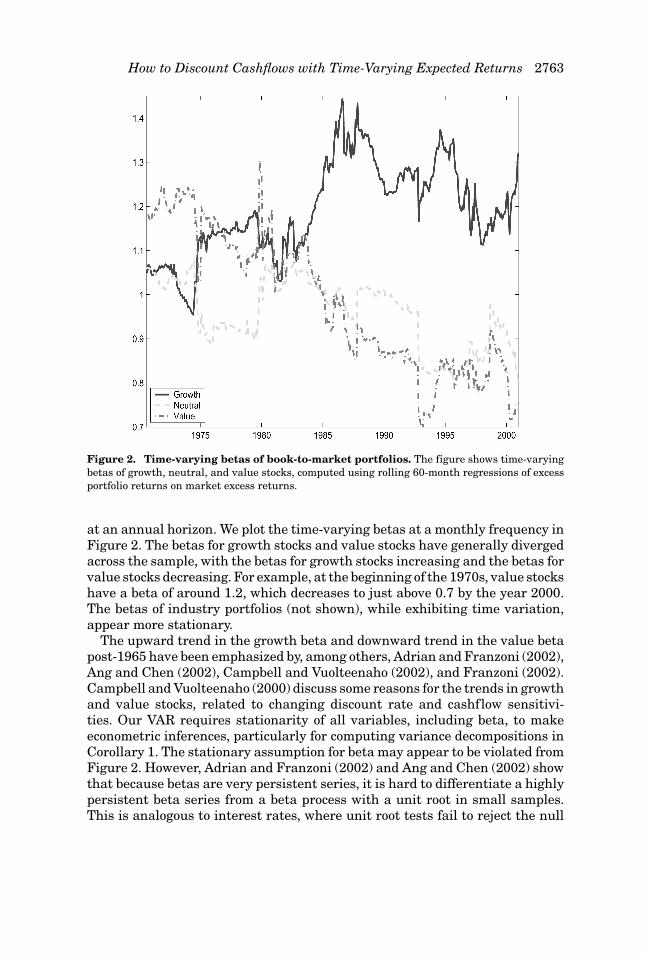
Figure 2. Time-varying betas of book-to-market portfolios. The figure shows time-varyingbetas of growth, neutral, and value stocks, computed using rolling 60-month regressions of excessportfolio returns on market excess returns.
at an annual horizon. We plot the time-varying betas at a monthly frequency inFigure 2. The betas for growth stocks and value stocks have generally divergedacross the sample, with the betas for growth stocks increasing and the betas forvalue stocks decreasing. For example, at the beginning of the 1970s, value stockshave a beta of around 1.2, which decreases to just above 0.7 by the year 2000.The betas of industry portfolios (not shown), while exhibiting time variation,appear more stationary.
The upward trend in the growth beta and downward trend in the value betapost-1965 have been emphasized by, among others, Adrian and Franzoni (2002),Ang and Chen (2002), Campbell and Vuolteenaho (2002), and Franzoni (2002).Campbell and Vuolteenaho (2000) discuss some reasons for the trends in growthand value stocks, related to changing discount rate and cashflow sensitivi-ties. Our VAR requires stationarity of all variables, including beta, to makeeconometric inferences, particularly for computing variance decompositions inCorollary 1. The stationary assumption for beta may appear to be violated fromFigure 2. However, Adrian and Franzoni (2002) and Ang and Chen (2002) showthat because betas are very persistent series, it is hard to differentiate a highlypersistent beta series from a beta process with a unit root in small samples.This is analogous to interest rates, where unit root tests fail to reject the null

2764 The Journal of Finance
of a unit root in small samples because of low power, but term structure modelsrequire the short rate to be a stationary process.
We list the estimates of the regression (27) in Panel B of Table I. The coeffi-cient on the interest rate is negative, so higher interest rates cause decreasesin market risk premiums. This is the same sign found by many studies sinceFama and Schwert (1977). However, while Ang and Bekaert (2002) and Camp-bell and Yogo (2002) document strong predictive power of the short rate atmonthly horizons, the significance is greatly reduced at an annual horizon.Lettau and Ludvigson (2001) find that, in-sample, cayt significantly predictsmarket risk premiums with a positive sign. However, without look-ahead biasat an annual horizon, the predictive power of cayt is reduced. Nevertheless, itis the same sign found by Lettau and Ludvigson (2001).
Since the risk premium is a function of instrumental variables, it is possibleto infer the variation of the risk premium from the regression coefficients brand bcay in (27) using
σλ =√
ζ ′�X ζ , (28)
where ζ = (000brbcay0)′ and �X is the unconditional covariance matrix of Xt.From the estimated parameters in Panel B of Table I, the unconditional volatil-ity of the risk premium is 2.66%, and the risk premium has an autocorrelationof 0.54.
IV. The Calibrated Term Structure of Expected Returns
In this section, we concentrate on presenting the term structure of discountrates for the growth, neutral, and value portfolios. The term structure of dis-count rates from these portfolios are representative of the general picture ofthe spot expected returns from other portfolios. However, we look at mispric-ings from valuations incorporating time-varying expected returns from bothbook-to-market and industry portfolios.
A. VAR Estimation Results
We report some selected VAR estimation results in Table II for growth, neu-tral, and value stocks. The average industry refers to a pooled estimation of theVAR across all industry portfolios. Table II shows that there are some signif-icant feedback effects from the instruments rt, cayt, and �pot to growth ratesand time-varying betas. For example, for growth (value) stocks, lagged interestrates (cayt) predict future cashflows, and, for neutral stocks, interest rates and�pot predict growth rates and betas. For the average industry, rt, cayt, and πtsignificantly predict dividend growth and betas.
In Table II, while cashflows gt are predictable, particularly by short ratesand cayt for industry portfolios, cashflows have weak forecasting ability for thevariables driving conditional expected returns, βt, rt, and cayt. The VAR results

How to Discount Cashflows with Time-Varying Expected Returns 2765
Table IICompanion Form Φ Parameter Estimates
The table reports estimates of the companion form � of the VAR in equation (7). The estimation isdone at an annual horizon, using monthly (overlapping) data. For the average industry results, wepool data across all industries. Standard errors are computed using Newey–West (1987) 12 lags.Parameters significant at the 95% level are denoted in bold. The sample period is July 1970 toDecember 2000 for the book-to-market sorted portfolios and from January 1970 to December 2000for the industry portfolios.
gt βt �pot rt cayt πt
Growth stocks gt −0.35 0.45 0.37 −4.06 1.86 1.69B/M Decile = 1 (0.17) (0.32) (0.32) (1.43) (2.40) (1.23)
βt −0.00 0.68 −0.08 0.48 0.85 −0.74(0.03) (0.11) (0.08) (0.48) (0.54) (0.44)
�pot 0.04 0.11 −0.37 0.71 −0.19 −0.31(0.02) (0.15) (0.18) (0.58) (1.42) (0.68)
rt −0.00 −0.02 −0.04 0.60 0.21 0.14(0.00) (0.03) (0.03) (0.12) (0.18) (0.14)
cayt 0.00 0.03 −0.01 0.09 0.54 0.07(0.01) (0.01) (0.02) (0.08) (0.09) (0.05)
πt 0.01 −0.04 −0.03 −0.09 0.07 0.73(0.00) (0.04) (0.03) (0.16) (0.16) (0.15)
Neutal stocks gt −0.13 0.03 0.61 −1.60 −0.06 1.22B/M Decile = 6 (0.18) (0.27) (0.24) (0.91) (1.58) (1.12)
βt −0.00 0.57 −0.11 1.20 −0.23 −0.10(0.05) (0.12) (0.09) (0.38) (0.50) (0.34)
�pot 0.12 −0.02 −0.32 0.83 0.11 −0.38(0.07) (0.10) (0.13) (0.51) (0.57) (0.34)
rt 0.02 0.02 −0.01 0.58 0.12 0.14(0.01) (0.03) (0.04) (0.13) (0.15) (0.12)
cayt 0.00 0.01 −0.00 0.06 0.65 0.02(0.01) (0.02) (0.01) (0.08) (0.08) (0.05)
πt 0.00 0.03 −0.01 −0.16 −0.09 0.81(0.02) (0.05) (0.03) (0.18) (0.20) (0.15)
Value stocks gt −0.06 0.20 −0.16 1.37 5.83 −1.26B/M Decile = 10 (0.12) (0.20) (0.13) (1.19) (1.50) (1.48)
βt −0.04 0.84 −0.12 −0.12 0.40 0.74(0.04) (0.07) (0.07) (0.42) (0.82) (0.44)
�pot 0.16 −0.15 −0.43 1.16 0.72 0.44(0.05) (0.14) (0.20) (0.42) (1.09) (0.46)
rt 0.01 0.02 −0.04 0.57 0.16 0.16(0.01) (0.01) (0.01) (0.11) (0.14) (0.14)
cayt 0.00 0.00 0.01 0.06 0.63 0.01(0.00) (0.01) (0.01) (0.06) (0.09) (0.05)
πt 0.03 0.05 −0.04 −0.17 −0.08 0.65(0.01) (0.02) (0.01) (0.14) (0.15) (0.14)
(Continued)
2766 The Journal of Finance
Table II—Continued
gt βt �pot rt cayt πt
Average industry gt −0.16 −0.04 0.19 −0.75 1.41 1.02(0.24) (0.19) (0.22) (0.00) (0.00) (0.00)
βt 0.00 0.91 −0.02 −0.03 0.10 0.10(0.01) (0.13) (0.26) (0.02) (0.00) (0.00)
�pot −0.01 0.02 −0.45 0.40 0.40 0.14(0.01) (0.02) (0.14) (0.02) (0.01) (0.00)
rt 0.00 0.00 −0.00 0.58 0.11 0.18(0.01) (0.03) (0.00) (0.02) (0.01) (0.02)
cayt 0.00 0.00 −0.00 0.07 0.64 0.02(0.01) (0.01) (0.00) (0.00) (0.01) (0.03)
πt 0.01 0.01 −0.00 −0.11 −0.11 0.80(0.11) (0.08) (0.00) (0.00) (0.00) (0.02)
for the “Average Industry” pools across all 45 industry portfolios and does notfind any evidence of predictability by cashflows. Hence, we might expect thefeedback effect of cashflows on time-varying expected returns to be weak.
B. Discount Curves
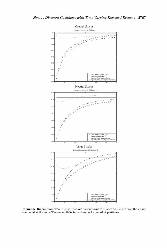
Figure 3 plots the term structure of discount rates µt(n) for growth, neutral,and value stocks. The discount curve for the full model is shown in circles. Atthe end of December 2000, the term structure of discount rates is upward slop-ing. At December 2000, the risk-free rate and cayt both predict low-conditionalexpected returns for the market. This markedly lowers the short end of thediscount curve. Since the risk premium is mean-reverting, the discount ratesincrease with maturity and asymptote to a constant.6
In Figure 3, the spot discount curve for growth stocks lies below the discountcurve for value stocks. However, in Figure 2, the betas of growth stocks arehigher than value stocks. The discrepancy is due to two reasons. First, theconstant α term in equation (4) is negative (positive) for growth (value) stocks.This reflects the well-known value effect (see, e.g., Fama and French (1993))and brings down the spot discount curve for growth stocks relative to valuestocks. Second, the discount curves also incorporate the effect of cashflows ontime-varying expected returns in the VAR in equation (7).
Figure 3 also superimposes the discount curves for the three special cases.First, the term structure of discount rates for an unconditional CAPM is a hor-izontal line, since it is constant across horizon. Second, the shape of the termstructure of discount rates ignoring the time variation in beta is similar to theshape of the full model, particularly for growth and neutral stocks. There is afaster gradient for value stocks, but the similarities may result in a relatively
6 As n → ∞, µ(n) → µ, where µ is a constant. This is proved in the Appendix.
How to Discount Cashflows with Time-Varying Expected Returns 2767
Growth Stocks
0 5 10 15 20 25 300.02
0.03
0.04
0.05
0.06
0.07
0.08
0.09
0.1
Discount Curve µt(n) for BM Decile = 1
Spot Discount Curve µt(n)
Unconditional CAPM Ignoring Time−Varying Betas Ignoring Time−Varying Risk Premiums
Neutral Stocks
0 5 10 15 20 25 300.06
0.07
0.08
0.09
0.1
0.11
0.12
0.13
Discount Curve µt(n) for BM Decile = 6
Spot Discount Curve µt(n)
Unconditional CAPM Ignoring Time−Varying Betas Ignoring Time−Varying Risk Premiums
Value Stocks
0 5 10 15 20 25 300.09
0.1
0.11
0.12
0.13
0.14
0.15
0.16
Discount Curve µt(n) for BM Decile = 10
Spot Discount Curve µt(n)
Unconditional CAPM Ignoring Time−Varying Betas Ignoring Time−Varying Risk Premiums
Figure 3. Discount curves. The figure shows discount curves µt(n), with n in years on the x-axis,computed at the end of December 2000 for various book-to-market portfolios.
2768 The Journal of Finance
small degree of misvaluation if we ignore the time variation in beta. However,there is a large change in the shape of the term structure when we ignore timevariation in the risk premium. In this case, the discount curves are much higherbecause when we ignore time variation of the risk premium, we cannot capturethe low-conditional expected returns of the market portfolio at December 2000.For growth and value stocks, the term structure of discount rates ignoring thetime-varying risk premium takes on inverse humped shapes, illustrating someof the variety of the different shapes the discount curves may assume.
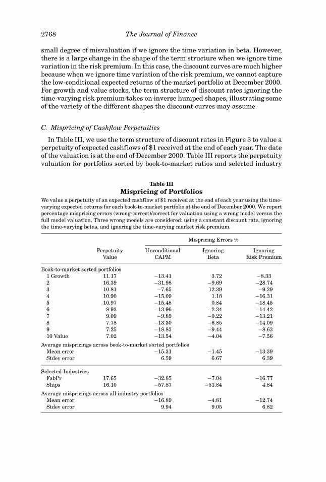
C. Mispricing of Cashflow Perpetuities
In Table III, we use the term structure of discount rates in Figure 3 to value aperpetuity of expected cashflows of $1 received at the end of each year. The dateof the valuation is at the end of December 2000. Table III reports the perpetuityvaluation for portfolios sorted by book-to-market ratios and selected industry
Table IIIMispricing of Portfolios
We value a perpetuity of an expected cashflow of $1 received at the end of each year using the time-varying expected returns for each book-to-market portfolio at the end of December 2000. We reportpercentage mispricing errors (wrong-correct)/correct for valuation using a wrong model versus thefull model valuation. Three wrong models are considered: using a constant discount rate, ignoringthe time-varying betas, and ignoring the time-varying market risk premium.
Mispricing Errors %
Perpetuity Unconditional Ignoring IgnoringValue CAPM Beta Risk Premium
Book-to-market sorted portfolios1 Growth 11.17 −13.41 3.72 −8.332 16.39 −31.98 −9.69 −28.743 10.81 −7.65 12.39 −9.294 10.90 −15.09 1.18 −16.315 10.97 −15.48 0.84 −18.456 8.93 −13.96 −2.34 −14.427 9.09 −9.89 −0.22 −13.218 7.78 −13.30 −6.85 −14.099 7.25 −18.83 −9.44 −8.6310 Value 7.02 −13.54 −4.04 −7.56
Average mispricings across book-to-market sorted portfoliosMean error −15.31 −1.45 −13.39Stdev error 6.59 6.67 6.39
Selected IndustriesFabPr 17.65 −32.85 −7.04 −16.77Ships 16.10 −57.87 −51.84 4.84
Average mispricings across all industry portfoliosMean error −16.89 −4.81 −12.74Stdev error 9.94 9.05 6.82
How to Discount Cashflows with Time-Varying Expected Returns 2769
portfolios. Table III also illustrates the large misvaluations that may result by(counter-factually) assuming expected returns are constant, ignoring the factthat betas vary over time, or ignoring the time variation in the market riskpremium.
To compute the perpetuity values, we set Et[Dt+s] = 1 for each horizon s inequation (16). We value this perpetuity within each book-to-market decile or in-dustry, under our model with time-varying conditional expected returns. Theseperpetuities do not represent the prices of any real firm or project because theyare not actual forecasted cashflows. By keeping expected cashflows constantacross the portfolios, we directly illustrate the role that time-varying expectedreturns play, without having to control for cashflow effects across industries inthe numerator. However, in the denominator, the discount rates still incorporatethe effects of cashflows on time-varying expected returns in the VAR.
After computing perpetuity values from our model, we compute perpetuityvalues from three mispricings relative to the true model: (1) using a constantdiscount rate from an unconditional CAPM, which is a traditional DDM val-uation; (2) ignoring the time variation in β but recognizing the market riskpremium is predictable; and (3) ignoring the predictability of the market riskpremium, but taking into account time-varying β. We report the mispricings aspercentage errors:
mispricing error = wrong − correctcorrect
, (29)
where “correct” is the perpetuity value from the full valuation and “wrong” isthe perpetuity value from each special case.
We turn first to the results in Table III for the book-to-market portfolios. Theperpetuity values are from the baseline case of time-varying short rates, betas,and risk premiums. There is a general pattern of high perpetuity values forgrowth stocks to low perpetuity values for value stocks, but the pattern is notstrictly monotonic. This follows from the low (high) discount rates for growth(value) stocks in Figure 3. The perpetuity values are almost monotonic, exceptfor the second book-to-market decile. This is mostly due to the more negativealpha for the second decile (−0.03) than the first decile (−0.02). In addition,the growth firms (decile 1) have low payout ratios. This may understate thepotential predictability of discount rates by cashflows.
The second column in Table III reports large mispricing errors from apply-ing a DDM, with a mean error of −15%. The maximum mispricing, in absoluteterms, is −32% for the second book-to-market decile portfolio. The DDM pro-duces much higher cashflow perpetuity values, because at the end of December2000, the conditional expected returns from our model are low, while the un-conditional expected return implied by the CAPM is much higher.
The case presented in the column labeled “Ignoring Beta” in Table IIIallows for time-varying expected returns, but only through the risk premiumand short rate. Ignoring time-varying betas results in overall smaller mispric-ings, but at this point in time the effect of time-varying betas can still be large(e.g., 12% for the third book-to-market decile portfolio). The largest effect in

2770 The Journal of Finance
misspecifying the expected return at December 2000 comes from ignoring thetime-varying market return, in the last column, rather than misspecifying thetime-varying beta. Like the DDM, ignoring variation in the risk premium pro-duces consistently higher values of the cashflow perpetuity relative to the base-line case. This is because, as the level of the market is very high at December2000, the conditional risk premium is very low. When we use the average riskpremium, we ignore this effect.
The same picture is repeated for the industry portfolios, except the extrememispricings are even larger. At December 2000, the discount rates for individ-ual industries take on a similar shape to the discount rates for book-to-marketportfolios in Figure 3, because of the low-conditional risk premium versus therelatively high-unconditional expected return. Table III lists the two portfo-lios with the two largest absolute pricing errors from the unconditional CAPM,which are the ship industry (−58%) and fabricated products (−33%), respec-tively. The ship industry has a low beta at December 2000 (0.63), which causesit to have a very high perpetuity value. The unconditional beta is much higher(1.06), which means that using the DDM with the unconditional CAPM resultsin a large incorrect valuation. On average, using an unconditional CAPM forvaluation produces a mispricing of −17% across all industry portfolios. Likethe book-to-market portfolios, ignoring the risk premium at December 2000produces larger misvaluations on average (−13%) than ignoring the time vari-ation of beta (−5%). In summary, the effect of time-varying expected returnson valuation is important.
D. Variance Decompositions
That ignoring time-varying expected returns, or some component of time-varying expected returns, produces different valuations than the DDM is nosurprise. What is more economically interesting is to investigate what is drivingthe time variation in the discount rates. We examine this by applying Corollary2 to compute variance decompositions of the spot expected returns.
We first illustrate the volatility of the spot expected returns,√
var(µt(n)), ateach maturity in the left column of Figure 4. As the maturity increases, thevolatility of the discount rates tends to zero. This is because as n → ∞, µt(n)approaches a constant because of stationarity, so var(µt(n)) → 0. At a 30-yearhorizon, the µt(30) discount rate still has a volatility above 2.5% for growthand neutral stocks, and above 7.0% for value stocks. While the volatility curvemust eventually approach zero, it need not do so monotonically. In particular,for value stocks, there is a strong hump-shape, starting from around 4.7% at a1-year horizon, increasing to near 8.0% at 13 years before starting to decline.The strong hump in
√var(µt(n)) for value stocks compared to growth and neu-
tral stocks is due to the much larger persistence of the value betas (0.84 com-pared to 0.68 (0.57) for growth (neutral) stocks in the VAR estimates of Table II).Note that the current beta is known in today’s conditional expected return. Ashock to the beta only takes effect next period and the more persistent the beta,the larger the contribution to the variance of the discount rate.

How to Discount Cashflows with Time-Varying Expected Returns 2771
Growth Stocks
0 5 10 15 20 25 300.02
0.025
0.03
0.035
0.04
0.045
0.05Discount Curve Volatility
0 5 10 15 20 25 30−0.4
−0.2
0
0.2
0.4
0.6
0.8
1Variance Decomposition for BM Decile = 1
Cashflows Beta Risk−Free RatesRisk Premium
Neutral Stocks
0 5 10 15 20 25 300.025
0.03
0.035
0.04
0.045
0.05Discount Curve Volatility
0 5 10 15 20 25 300
0.1
0.2
0.3
0.4
0.5
0.6
0.7
0.8
0.9Variance Decomposition for BM Decile = 6
Cashflows Beta Risk−Free RatesRisk Premium
Value Stocks
0 5 10 15 20 25 300.045
0.05
0.055
0.06
0.065
0.07
0.075
0.08Discount Curve Volatility
0 5 10 15 20 25 30−0.2
0
0.2
0.4
0.6
0.8
1
1.2Variance Decomposition for BM Decile = 10
Cashflows Beta Risk−Free RatesRisk Premium
Figure 4. Variance decomposition for the term structure of discount rates. The left-hand column plots
√var(µt (n)), for each n on the x-axis. The right-hand column attributes the
var(µt(n)) into proportions due to dividend growth, beta, the risk-free rate, and the risk premium.The proportions double count the covariances and so do not sum to 1.

2772 The Journal of Finance
In the right-hand column of Figure 4, we decompose the variance of the dis-count rates. Our first result is that the time variation in cashflows makesonly a very small contribution to the variance of the spot expected returns. Weadd both the variance decomposition to gt and the variance decomposition to�pot together to determine the total variance decomposition to cashflows. Thesmall effect of cashflows on discount rates is expected, because cashflows orpayouts weakly predict the variables driving time-varying expected returns:time-varying betas, short rates, and cayt. The persistence of cashflows is alsovery low (see Table I), and so shocks to cashflows have little long-term effecton the variances of the discount factors.
Second, Figure 4 shows that at very short maturities, the attribution of thevariance of µt(n) to nominal risk-free rates is large, the attribution to the marketrisk premium is also large, and the attribution to beta is smaller than thevariance decomposition to risk-free rates or to the market risk premium. Forexample, for neutral stocks, approximately 65% of var(µt) is accounted for byrisk-free rates, 72% by the market risk premium, and 20% by time-varyingbeta. Hence, at short horizons, it is crucial to account for time-varying shortrates and risk premiums. The effect of beta is secondary.
Some intuition for this result can be gained by more closely examining theone-period expected return:
µt = rt + βtλt
= (rt + r − r) + (βt + β − β)(λt + λ − λ)
= const + (rt − rt) + β(λt − λ) + λ(βt − β) + (βt − β)(λt − λ), (30)
where r, β, and λ represent the unconditional means of nominal interest rates,beta, and risk premiums, respectively. Ignoring the covariance and other higher-order terms in (30), we have
var(µt) ≈ var(rt) + β2var(λt) + λ2var(βt). (31)
The variance of rt enters one for one and so has a large effect, but var(λt) andvar(βt) are scaled by the effects of β and λ. Since β is approximately 1, thevariance of the risk premium also has a large effect. However, the average logrisk premium in the data is of the order of 5%, which means that var(βt) has asmaller effect on the variance of µt than risk-free rates or market risk premia.For value stocks, the variance of betas is relatively large, allowing betas toaccount for up to 41% of the variance of µt(1), but this is still smaller than theone-period variance decompositions to risk-free rates (71%) and risk premia(72%).
Third, the variance decomposition of the risk premium decreases as n in-creases. While the time variation in the market is very important for the valueof short-term cashflows, we can pay less attention to the predictability of themarket premium for long-term cashflows. Mathematically, the risk premium isa linear function of the instrumental variables rt and cayt. The autocorrelationof rt is around 0.74 at an annual horizon, and cayt is much less autocorrelated
How to Discount Cashflows with Time-Varying Expected Returns 2773
(0.63 at an annual horizon). The risk premium is a linear function of both rtand cayt, and is less autocorrelated than the short rate (0.54). This means thatat long horizons, shocks to the risk premium are less persistent than shocks tothe short rate and other variables in the system, leading to a reduction in thevariance decomposition to the risk premium as n increases.7
Finally, the variance decomposition of the risk-free rate can increase or de-crease with horizon, and can dominate, or be dominated by the variance oftime-varying beta. For growth stocks, the attribution of var(µt(n)) to the in-terest rate only slightly decreases as n increases, while for value stocks therisk-free rate variance decomposition becomes much smaller at long horizons.Hence, growth stocks are more sensitive to movements in the nominal termstructure than value stocks. This is in line with intuition as growth stocks havefew short-term cashflows but potentially large long-term cashflows.
The mechanism by which the nominal risk-free rate or βt can dominate thevariance decomposition of var(µt(n)) at long horizons is due to the relative per-sistence of the interest rate versus beta and the size of the predictive coefficientsin the risk premium. Since the interest rate is very persistent, shocks to rt tendto dominate at long horizons unless the autocorrelation of beta is large enough,relative to the autocorrelation of real rates, to offset its effects. The autocorrela-tion of beta (0.86) is much larger than the autocorrelation of the beta of growthstocks (0.76), which allows the variance attribution to β to dominate at longhorizons for the value portfolio.
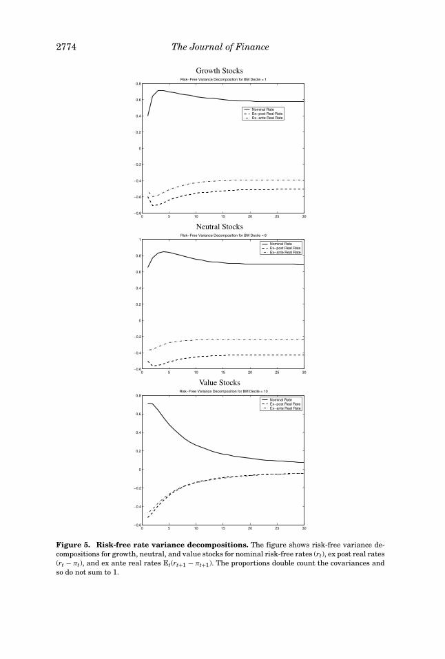
In Figure 5, we perform a more detailed variance decomposition of var(µt(n))to risk-free rates. Figure 5 repeats the variance decompositions to rt from Figure4 and also plots the variance decompositions to actual (or ex post) real ratesrt − πt and expected (or ex ante) real rates Et(rt+1 − πt+1). First, the variancedecompositions to nominal, actual, and expected real rates all follow the samepatterns in absolute magnitude. In particular, at short horizons, the variancedecompositions to real rates, like nominal rates, is large. The same intuitionfor these results for the nominal rate using the approximation in equation (31)also applies to the ex ante or ex post real rates.
Second, the variance decomposition to ex ante and ex post real rates isnegative, compared to the positive variance decompositions to rt. The rea-son is that while rt is unconditionally positively correlated with the otherstate variables, the actual and expected real rates are negatively correlatedwith the other state variables. For example, for value stocks, the correlationof rt with βt is 56%, whereas the correlation of rt − πt with βt is −25%, andthe correlation of Et(rt+1 − πt+1) with βt is −35%.8 By definition, the variance
7 If dividend yields are used instead of cayt, the variance decomposition to the risk premium fallsacross all horizons. While the dividend yield is more persistent than both the nominal or ex postreal risk-free rate, the predictive coefficient of the dividend yield in the risk premium regressionis almost zero in our sample.
8 The fact that the actual and expected real rates are negatively correlated with inflation (at−58% and −43%, respectively), while there is a positive correlation of nominal risk-free rates andinflation (70%), is the well-known Mundell (1963) and Tobin (1965) effect.
2774 The Journal of Finance
Growth Stocks
0 5 10 15 20 25 30−0.8
−0.6
−0.4
−0.2
0
0.2
0.4
0.6
0.8Risk−Free Variance Decomposition for BM Decile = 1
Nominal Rate Ex−post Real RateEx−ante Real Rate
Neutral Stocks
0 5 10 15 20 25 30−0.6
−0.4
−0.2
0
0.2
0.4
0.6
0.8
1Risk−Free Variance Decomposition for BM Decile = 6
Nominal Rate Ex−post Real RateEx−ante Real Rate
Value Stocks
0 5 10 15 20 25 30−0.6
−0.4
−0.2
0
0.2
0.4
0.6
0.8Risk−Free Variance Decomposition for BM Decile = 10
Nominal Rate Ex−post Real RateEx−ante Real Rate
Figure 5. Risk-free rate variance decompositions. The figure shows risk-free variance de-compositions for growth, neutral, and value stocks for nominal risk-free rates (rt), ex post real rates(rt − πt), and ex ante real rates Et(rt+1 − πt+1). The proportions double count the covariances andso do not sum to 1.

How to Discount Cashflows with Time-Varying Expected Returns 2775
decompositions to risk-free rates, ex ante real rates, and ex post real rates thatdo not count the covariances must be positive. Hence, the negative variancedecompositions result solely from the unconditional negative correlations ofreal rates with other state variables. Finally, the variance decompositions ofactual real rates are larger than the variance decompositions of ex ante realrates. This is expected, as the actual real rate comprises the ex-ante real rateplus unpredictable inflation noise.
V. Conclusion
Despite the strong evidence for time variation in the market risk premium,factor loadings, and risk-free rates, the main tool of valuation, the DDM, doesnot take into account any of these stylized facts. We develop a valuation method-ology that incorporates time-varying risk premiums, betas, and risk-free ratesby computing a series of discount rates that differ across maturity. The price ofa security has an analytical solution, which depends only on observable instru-ments.
For application to practical capital budgeting problems, we develop an ana-lytical, tractable term structure of discount rates. This series of discount ratesdiffers across maturity and can be applied to value a series of expected cash-flows. The discount curve is constructed in such a way to consistently modelthe dynamics of time-varying risk-free rates, betas, and risk premiums.
We estimate the term structure of discount rates for book-to-market and in-dustry portfolios, and find the effect of time variation in risk-free rates, betas,and risk premiums is large. By computing a variance decomposition of the dis-count rates, we show that at short horizons, investors should be most concernedwith the impact of time-varying interest rates and risk premiums for discount-ing cashflows. At long horizons, the time variation in risk-free rates or beta ismore important.
While we provide an easily applicable methodology for handling the effectsof time-varying risk premiums, risk-free rates, and beta, and demonstrate thatall these are important for valuation, future research must deal with somepractical issues. For example, parameter uncertainty in the predictability ofthe market risk premium and estimating betas will affect the capital budgetingproblem. Time-varying risk-free rates, betas, and risk premiums can only makepotential mispricings in these situations even larger.
Appendix A: Proof of Proposition 1
Before proving Proposition 1, we first prove a useful lemma:
LEMMA 1: Let ε be a K × 1 vector, where ε ∼ N(0, �), A a K × K matrix, and �
a symmetric K × K matrix. If (�−1 − 2�) is strictly positive definite, then
E[exp(Aε + ε′�ε)] = exp( − 1
2 ln det(I − 2��) + 12 A′(�−1 − 2�)−1 A
).

2776 The Journal of Finance
Proof:
E[exp(Aε + ε′�ε)] =∫
(2π )−K | det �|−1/2 exp(
−12
ε′�−1ε
)exp(A′ε + ε′�ε) d K ε
=∫
(2π )−K | det �|−1/2 exp(
−12
ε′(�−1 − 2�) + A′ε)
d K ε.
(A1)
If (�−1 − 2�) is strictly positive definite, then there exists a K × K lower trian-gular matrix M, det M = 0, such that (�−1 − 2�) = (MM′)−1. Substituting thisinto the above expression, we obtain
E[exp(Aε + ε′�ε)] =∫
(2π )−K |det �|−1/2 exp(
−12
ε′(M ′)−1M−1ε + A′ε)
d K ε.
(A2)
Now substitute u = M−1ε:
E[exp(Aε + ε′�ε)] =∫
(2π )−K |det �|−1/2 |det M | exp(
−12
u′u + A′Mu)
d K u
= |det M | |det �|−1/2 exp(
12
A′M M ′ A)
= |det M | |det �|−1/2 exp(
12
A′(�−1 − 2�)−1 A)
. (A3)
Finally, looking at the determinant terms we have
|det M | |det �|−1/2 =( |det(�−1 − 2�)−1|
|det �|)(1/2)
=(
1det �(�−1 − 2�)
)(1/2)
= exp(
−12
ln |det(I − 2��)|)
. (A4)
Substituting into (A3) we obtain the required result. Q.E.D.
Constantinides (1992) states a continuous-time version of Lemma 1, excepthis result is only for a univariate case.
To prove Proposition 1, consider one cashflow at time t + n in the term inequation (2) divided by Dt:
Et
[(n−1∏k=0
e−µt+k
)Dt+n
]/Dt . (A5)
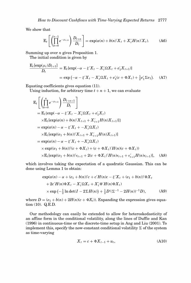
How to Discount Cashflows with Time-Varying Expected Returns 2777
We show that
Et
[(n−1∏k=0
e−µt+k
)Dt+n
Dt
]= exp(a(n) + b(n)′X t + X ′
t H(n)′X t). (A6)
Summing up over n gives Proposition 1.The initial condition is given by
Et[exp(µt)Dt+1]Dt
= Et[exp(−α − ξ ′X t − X ′t�X t + e′
1 X t+1)]
= exp(−α − ξ ′X t − X ′
t�X t + e′1(c + �X t) + 1
2 e′1�e1
). (A7)
Equating coefficients gives equation (11).Using induction, for arbitrary time t + n + 1, we can evaluate
Et
[(n∏
k=0
e−µt+k
)Dt+n+1
Dt
]
= Et{exp(−α − ξ ′X t − X ′t�X t + e′
1 X t)
×Et[exp(a(n) + b(n)′X t+1 + X ′t+1 H(n)X t+1)]}
= exp(a(n) − α − ξ ′X t + −X ′t�X t)
×Et[exp((e1 + b(n))′X t+1 + X ′t+1 H(n)X t+1)]
= exp(a(n) − α − ξ ′X t + −X ′t�X t)
× exp((e1 + b(n))′(c + �X t) + (c + �X t)′H(n)(c + �X t))
×Et[exp((e1 + b(n))′εt+1 + 2(c + �X t)′H(n)εt+1 + ε′t+1 H(n)εt+1)], (A8)
which involves taking the expectation of a quadratic Gaussian. This can bedone using Lemma 1 to obtain:
exp(a(n) − α + (e1 + b(n))′c + c′H(n)c − ξ ′X t + (e1 + b(n))′�X t
+ 2c′H(n)�X t − X ′t�X t + X ′
t�′H(n)�X t)
× exp(− 1
2 ln det(I − 2�H(n)) + 1
2 D′(�−1 − 2H(n))−1 D), (A9)
where D = (e1 + b(n) + 2H(n)(c + �Xt)). Expanding the expression gives equa-tion (10). Q.E.D.
Our methodology can easily be extended to allow for heteroskedasticity ofan affine form in the conditional volatility, along the lines of Duffie and Kan(1996) in continuous-time or the discrete-time setup in Ang and Liu (2001). Toimplement this, specify the now-constant conditional volatility � of the systemas time-varying
X t = c + �X t−1 + ut , (A10)
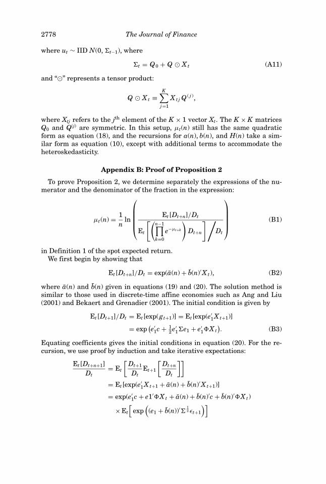
2778 The Journal of Finance
where ut ∼ IID N(0, �t−1), where
�t = Q0 + Q X t (A11)
and “” represents a tensor product:
Q X t ≡K∑
j=1
X t j Q ( j ),
where Xtj refers to the jth element of the K × 1 vector Xt. The K × K matricesQ0 and Q(j) are symmetric. In this setup, µt(n) still has the same quadraticform as equation (18), and the recursions for a(n), b(n), and H(n) take a sim-ilar form as equation (10), except with additional terms to accommodate theheteroskedasticity.
Appendix B: Proof of Proposition 2
To prove Proposition 2, we determine separately the expressions of the nu-merator and the denominator of the fraction in the expression:
µt(n) = 1n
ln
Et[Dt+n]/Dt
Et
[(n−1∏k=0
e−µt+k
)Dt+n
] /Dt
(B1)
in Definition 1 of the spot expected return.We first begin by showing that
Et[Dt+n]/Dt = exp(a(n) + b(n)′X t), (B2)
where a(n) and b(n) given in equations (19) and (20). The solution method issimilar to those used in discrete-time affine economies such as Ang and Liu(2001) and Bekaert and Grenadier (2001). The initial condition is given by
Et[Dt+1]/Dt = Et[exp(gt+1)] = Et[exp(e′1 X t+1)]
= exp(e′
1c + 12 e′
1�e1 + e′1�X t
). (B3)
Equating coefficients gives the initial conditions in equation (20). For the re-cursion, we use proof by induction and take iterative expectations:
Et[Dt+n+1]Dt
= Et
[Dt+1
DtEt+1
[Dt+n
Dt
]]
= Et[exp(e′1 X t+1 + a(n) + b(n)′X t+1)]
= exp(e′1c + e1′�X t + a(n) + b(n)′c + b(n)′�X t)
× Et
[exp
((e1 + b(n))′�
12 εt+1
)]

How to Discount Cashflows with Time-Varying Expected Returns 2779
= exp(e′
1c + a(n) + b(n)′c + (e1 + b(n))′�X t
+ 12 (e1 + b(n))′�(e1 + b(n))
). (B4)
Equating coefficients gives the recursion in equation (19).Proposition 1 shows that the denominator of (B1) has the form
Et
[(n−1∏k=0
e−µt+k
)Dt+n
Dt
]= exp(a(n) + b(n)′X t + X ′
t H(n)′X t), (B5)
where a(n), b(n), and H(n) follow the recursions in equation (10).This allows us to write µt(n) in equation (B1) as
µt(n) = A(n) + B(n)′X t + X ′tG(n)X t , (B6)
where A(n) = (a(n) − a(n))/n, B(n) = (b(n) − b(n))/n, and G(n) = −H(n)/n. Q.E.D.
Appendix C: Variance of the Discount Rate
Proof of Corollary 1: To compute the variance of the discount rate, var(µt(n)),in Corollary 1, we use the following lemma:
LEMMA 2: For an arbitrary matrix M, the following relationships are true (seeHarville (1997)):
∂
∂λln detM = tr
(M−1 ∂M
∂λ
)∂
∂λM−1 = −M−1 ∂M
∂λM−1. (C1)
Since, from Proposition 2, µt(n) = A(n) + B(n)′Xt + X ′tG(n)Xt we have
var(µt(n)) = B(n)′�X B(n) + var(X ′tG(n)X t). (C2)
We use a moment generating function to evaluate the last term. Let
g (λ) = E[exp(λε′Mε)]. (C3)
Then
var(ε′Mε) = ∂2 g (λ)∂λ2
∣∣∣λ=0
−(
∂ g (λ)∂λ
∣∣∣λ=0
)2
. (C4)
Using Lemma 1, we have
g (λ) = exp(− 1
2 ln det(I − 2λ�M )), (C5)
where � is the variance matrix of ε. Using Lemma 2, we have
∂
∂λg (λ) ln detM = g (λ)tr((I − 2λ�M )−1�M ), (C6)

2780 The Journal of Finance
and
∂2
∂λ2g (λ) ln detM = g (λ)
{(tr(I − 2λ�M )−1�M ))2
+ tr((I − 2λ�M )−12�M (I − 2λ�M )−1�M )}. (C7)
Therefore, we have
var(ε′Mε) = tr((�M )2), (C8)
evaluating equation (C5). Hence,
var(µt(n)) = B(n)′�X B(n) + 2tr((�X G(n))2) (C9)
given in equation (21). Q.E.D.
Proof of Corollary 2: From the definition of µt(n) = A(n) + B(n)′Xt + X ′tG(n)Xt,
we can write
µt(n) = (A(n) − B(n)′X ) + B(n)′(X t − X ) + (X t − X + X )′G(n)(X t − X + X )
= (A(n) − B(n)′X + X′G(n)X ) + (B(n) + 2G(n)X )′(X t − X )
+ (X t − X )′G(n)(X t − X ).
(C10)
Ignoring the quadratic term, we have
var(µt(n)) = (B(n) + 2G(n)X )′�X (B(n) + 2G(n)X ). (C11)
Since �X = L�ZL′, we can rewrite this expression as
var(µt(n)) = (B(n) + 2G(n)X )′L�Z L′(B(n) + 2G(n)X ), (C12)
giving us equation (22). Q.E.D.
Appendix D: Long-Term Discount Rates
It is possible to compute the long-term discount rate µ(∞) using the followingproposition:
PROPOSITION 3: Suppose the following limits exist:
limn→∞
a(n)n
= a∞,
limn→∞
a(n)n
= a∞,
limn→∞ b(n) = b∞,
limn→∞ b(n) = b∞,
limn→∞ H(n) = H∞,
(D1)

How to Discount Cashflows with Time-Varying Expected Returns 2781
then the long-term discount rate µ(∞) is given by
µ(∞) = (a∞ − a∞), (D2)
where
a∞ = e′1c + b′
∞c + 12 (e1 + b∞)′�(e1 + b∞),
a∞ = −α + (e1 + b∞)′c + c′H∞c − 12 ln det(I − 2�H∞). (D3)
Given H∞, b∞, and b∞ are given by
b∞ = (I − �′)−1�′e1,
b∞ = (I − �′ − 2�′H∞(�−1 − 2H∞)−1)−1
× (−ξ + �′e1 + 2�′H∞c + 2�′H∞(�−1 − 2H∞)−1(e1 + 2H∞c)). (D4)
The matrix H∞ solves the relation
H∞ = −� + �′H∞� + 2�′H∞(�−1 − 2H∞)−1 H∞�. (D5)
In practice, it is easy to solve for H∞ by iterating the recursion for H(n) inequation (10) to a very large number. After n > 100 years, H(n) is constant.Once H∞ is found, a∞ and a∞ are closed form.
REFERENCESAdrian, Tobias, and Francesco Franzoni, 2002, Learning about beta: An explanation of the value
premium, Working paper, MIT.Ahn, Dong Hyun, Robert F. Dittmar, and A. Ronald Gallant, 2002, Quadratic term structure models:
Theory and evidence, Review of Financial Studies 15, 243–288.Ang, Andrew, and Geert Bekaert, 2002, Stock return predictability: Is it there? Working paper,
Columbia Business School.Ang, Andrew, and Joseph Chen, 2002, CAPM over the long-run: 1926–2001, Working paper,
Columbia Business School.Ang, Andrew, and Jun Liu, 2001, A general affine earnings valuation model, Review of Accounting
Studies 6, 397–425.Bakshi, Gurdip, and Zhiwu Chen, 2001, Stock valuation in dynamic economies, Working paper,
Yale University.Bekaert, Geert, and Steve Grenadier, 2001, Stock and bond pricing in an affine economy, Working
paper, Columbia Business School.Berk, Jonathan B., Richard C. Green, and Vasant Naik, 1999, Optimal investment, growth options,
and security returns, Journal of Finance, 54, 1153–1607.Brennan, Michael J., 1997, The term structure of discount rates, Financial Management 26, 81–90.Brennan, Michael J., and Yihong Xia, 2001, TAY’s as good as CAY, Working paper, Wharton.Campbell, John Y., 1987, Stock returns and the term structure, Journal of Financial Economics
18, 373–399.Campbell, John Y., and Robert J. Shiller, 1988a, Stock prices, earnings and expected dividends,
Journal of Finance 43, 661–676.Campbell, John Y., and Robert J. Shiller, 1988b, The dividend–price ratio and expectations of future
dividends and discount factors, Review of Financial Studies 1, 195–228.Campbell, John Y., and Luis M. Viceira, 1999, Consumption and portfolio decisions when expected
returns are time varying, Quarterly Journal of Economics 114, 433–495.
2782 The Journal of Finance
Campbell, John Y., and Tuomo Vuolteenaho, 2002, Bad beta, good beta, Working paper, HarvardUniversity.
Campbell, John Y., and Motohiro Yogo, 2002, Efficient tests of stock return predictability, Workingpaper, Harvard University.
Cochrane, John H., 1996, A cross-sectional test of an investment-based asset pricing model, Journalof Political Economy 104, 572–621.
Constantinides, George M., 1992, A theory of the nominal term structure of interest rates, Reviewof Financial Studies 5, 531–552.
Duffie, Darrel, and Rui Kan, 1996, A yield-factor model of interest rates, Mathematical Finance 6,379–406.
Fama, Eugene F., 1996, Discounting under uncertainty, Journal of Business 69, 415–428.Fama, Eugene F., and Kenneth R. French, 1993, Common risk factors in the returns on stocks and
bonds, Journal of Financial Economics 25, 23–49.Fama, Eugene F., and Kenneth R. French, 1997, Industry costs of equity, Journal of Financial
Economics 43, 153–193.Fama, Eugene F., and Kenneth R. French, 2002, The equity premium, Journal of Finance 57,
637–659.Fama, Eugene F., and James MacBeth, 1973, Risk, return, and equilibrium: Empirical tests, Jour-
nal of Political Economy 81, 607–636.Fama, Eugene F., and G. William Schwert, 1977, Asset returns and inflation, Journal of Financial
Economics 5, 115–146.Ferson, Wayne E., and Campbell R. Harvey, 1991, The variation of economic risk premiums, Journal
of Political Economy 99, 385–415.Ferson, Wayne E., and Campbell R. Harvey, 1993, The risk and predictability of international
equity returns, Review of Financial Studies 6, 527–566.Ferson, Wayne E., and Campbell R. Harvey, 1999, Conditioning variables and the cross section of
stock returns, Journal of Finance 54, 1325–1360.Ferson, Wayne E., and Robert A. Korajczyk, 1995, Do arbitrage pricing models explain the pre-
dictability of stock returns? Journal of Business 68, 309–349.Franzoni, Francesco, 2002, Where is beta going? The riskiness of value and small stocks, Working
paper, MIT.Goyal, Amit, and Ivo Welch, 2003, The myth of predictability: Does the dividend yield forecast the
equity premium? Management Science 49, 639–654.Graham, John R., and Campbell R. Harvey, 2001, The theory and practice of corporate finance:
Evidence from the field, Journal of Financial Economics 61, 1–28.Hahn, Jaehoon, and Hayong Lee, 2002, On the estimation of the consumption–wealth ratio: Cointe-
grating parameter instability and its implications for stock return forecasting, Working paper,University of Washington.
Harvey, Campbell R., 1989, Time-varying conditional covariances in tests of asset pricing models,Journal of Financial Economics 24, 289–317.
Harville, David A., 1997, Matrix Algebra from a Statistician’s Perspective (Springer-Verlag, NewYork).
Hodrick, Robert J., 1992, Dividend yields and expected stock returns: Alternative procedures forinference and measurement, Review of Financial Studies 5, 357–386.
Jagannathan, Ravi, Ellen R. McGrattan, and Anna Scherbina, 2001, The declining U.S. equitypremium, Quarterly Review, Federal Reserve Bank of Minneapolis 24, Fall, 3–19.
Jagannathan, Ravi, and Zhenyu Wang, 1996, The conditional CAPM and the cross-section of ex-pected returns, Journal of Finance 51, 3–53.
Jostova, Gergana, and Alex Philipov, 2002, Bayesian analysis of stochastic betas, Working paper,Boston College.
Keim, Donald B., and Robert F. Stambaugh, 1986, Predicting returns in the stock and bond markets,Journal of Financial Economics 17, 357–390.
Kim, Tong S., and Edward Omberg, 1996, Dynamic nonmyopic portfolio behavior, Review of Finan-cial Studies 9, 141–161.

How to Discount Cashflows with Time-Varying Expected Returns 2783
Lee, Charles M.C., James N. Myers, and Bhaskaran Swaminathan, 1999, What is the intrinsicvalue of the Dow? Journal of Finance 64, 1693–1741.
Lettau, Martin, and Sydney Ludvigson, 2001, Consumption, aggregate wealth, and expected re-turns, Journal of Finance 56, 815–849.
Lettau, Martin, and Sydney Ludvigson, 2002, Measuring and modeling variation in the risk-returntradeoff, Working paper, NYU.
Liu, Jun, 1999, Portfolio selection in stochastic environments, Working paper, UCLA.Menzly, Lior, Tano Santos, and Pietro Veronesi, 2003, The time series of the cross section of asset
prices, Working paper, University of Chicago.Mundell, Robert, 1963, Inflation and real interest, Journal of Political Economy 71, 280–283.Newey, Whitney, and Kenneth West, 1987, A simple, positive semi-definite, heteroskedasticity and
autocorrelation consistent covariance matrix, Econometrica 55, 703–708.Shanken, Jay, 1990, Intertemporal asset pricing—An empirical investigation, Journal of Econo-
metrics 45, 99–120.Tobin, James, 1965, Money and economic growth, Econometrica 33, 671–684.Vuolteenaho, Tuomo, 2002, What drives firm-level stock returns?, Journal of Finance 57, 233–264.

2784


![Chap18[1] the Statement of Cashflows](https://img.pdfslide.us/doc/110x75/55cf9942550346d0339c7445/chap181-the-statement-of-cashflows.jpg)