Embed Size (px)
Citation preview

VERSION 12.0
PART NUMBER120VIBTR-01
Visit us at: www.adams.com
ADAMS Vibration Training Guide

U.S. Government Restricted Rights: If the Software and Documentation are provided in connection with a
government contract, then they are provided with RESTRICTED RIGHTS. Use, duplication or disclosure is
subject to restrictions stated in paragraph (c)(1)(ii) of the Rights in Technical Data and Computer Software
clause at 252.227-7013. Mechanical Dynamics, Incorporated, 2300 Traverwood Drive, Ann Arbor, Michigan
48105.
The information in this document is furnished for informational use only, may be revised from time to time,
and should not be construed as a commitment by Mechanical Dynamics, Incorporated. Mechanical
Dynamics, Incorporated, assumes no responsibility or liability for any errors or inaccuracies that may
appear in this document.
This document contains proprietary and copyrighted information. Mechanical Dynamics, Incorporated
permits licensees of ADAMS® software products to print out or copy this document or portions thereof
solely for internal use in connection with the licensed software. No part of this document may be copied for
any other purpose or distributed or translated into any other language without the prior written permission of
Mechanical Dynamics, Incorporated.
©2002 by Mechanical Dynamics, Incorporated. All rights reserved. Printed in the United States of America.
ADAMS ® is a registered United States trademark of Mechanical Dynamics, Incorporated.
All other product names are trademarks of their respective companies.

3
Contents
Welcome to ADAMS/Vibration Training 5About MSC.Software 6Course Overview 7Getting Help in Class 8Getting Help at Your Job Site 11
Introduction 13
Overview 14What is ADAMS/Vibration? 20Instrumenting the Model 21Input Channels and Actuators 22Swept Sine 23Output Channels 24Forced-Vibration Analysis Specification 25Workshop 1—Introduction 26
Validation Example 39
Vibration Analysis Methods Comparison 40More Details of Time-Domain Method 41Post-Processing 42Workshop 2—Validation Example 43
Power Spectral Density (PSD) 57
PSD—What is it? 58PSD Actuator 59Workshop 3—Power Spectral Density (PSD) Input 60
User-Defined Input 77
Overview 78Workshop 4—User-Specified Vibration Actuators 79
Rotating Mass Vibration Actuator 91
Rotating Mass 92Modal Energy Computation 96Workshop 5—Rotating Mass Vibration Actuator 97

4 Contents
CONTENTS...
Vibration of Flexible Bodies 115
Overview 116Operating Point 117Workshop 6—Vibration of Flexible Bodies 118
Using Design Evaluation to Minimize Frequency Response 131
What ADAMS/View Requires 132Types of ADAMS/Vibration Macros 133Design Objective Details 134Dialog Box Cascade 135Other Considerations 136Workshop 7—Design Evaluation 137
Theory 153
Introduction 154Vibration Actuators 155Analysis Methods 157
Answer Key 159
Answer Key 160

5
WELCOME TO ADAMS/VIBRATION TRAINING
Welcome to ADAMS/Vibration training. In this course, you learn how to use ADAMS/Vibration to create input channels, output channels, and vibration actuators. You�ll also learn how to run various types of analyses and perform postprocessing tasks.
What�s in this section:� About MSC.Software, 6
� Course Overview, 7
� Getting Help in Class, 8
� Getting Help at Your Job Site, 11

6 Welcome to ADAMS/Vibration Training
About MSC.Software
Find a list of ADAMS products at: � http://www.adams.com/mdi/product/modules.htm
Learn about the ADAMS�CAD/CAM/CAE integration at:� http://www.adams.com/mdi/product/partner.htm
Find additional training at:� http://support.adams.com/training/training.html
� Or your local support center

Welcome to ADAMS/Vibration Training 7
Course Overview�
Lecture
Hands-on workshops
Theory
�

8 Welcome to ADAMS/Vibration Training
Getting Help in Class
Online help To access the online help:
� Press F1 when a dialog box is active
� From the Help menu, select ADAMS/Vibration Help
Referencing the online help�� While working in any ADAMS/Vibration dialog box, you can press F1 to display online
help specific to that dialog box.
� Once the online help is displayed, you can also search for any terms you are looking for or browse through the index or table of contents.
�Demonstrate the online help. Press F1.Read the FAQ for online help.Note: For ADAMS/Flex, only the Create a Flexible Body dialog box has help.Mention to students that they can search the online help as shown on this page. If they don�t find what they are looking for, they can search the pdf guides as shown on page 10.
Enter a search term Select, and then select the Index tab

Welcome to ADAMS/Vibration Training 9
Getting Help in Class...
Online guides To access the online guides:
� From the Help menu, select ADAMS/Vibration Guides
� To display the ADAMS products home page, Road Map to ADAMS Documentation, from the Help menu, select Online Guides
Help on help Access help on help by selecting the:
� Help on Help bookmark in any ADAMS guide
� Help tool on the Road Map to ADAMS Documentation or the Road Map to ADAMS/View Documentation
Course CDThe course CD includes the files you will need to complete each workshop, a set of completed workshop files, the course guide in pdf format, as well as the related ADAMS/Vibration documentation.

10 Welcome to ADAMS/Vibration Training
Getting Help in Class...
Doing global searches on any online ADAMS guide�
� Demo the search and select text functions in Acrobat Reader:
� Search in displayed guide:
� Global search:
� Select text:
� Zoom in:
� Zoom out: press Ctrl +

Welcome to ADAMS/Vibration Training 11
Getting Help at Your Job Site
�Personalized news and informationTo receive more consistent, targeted news and information, go to http://my.adams.com/cgi-bin/myadams.cgi, a Web personalization site. Some of the news channels this site provides are:
� Case studies - Practical application stories
� Events - Seminars, user conferences, and trade shows
� Product alerts - Known problems, workarounds, and Service Packs
Technical support To find your support center, go to http://support.adams.com/services/support/support_centers.shtm
To read the Service Level Agreement, go to http://support.adams.com/services/support/sla_agree.shtm
knowledge base
Go to http://support.adams.com/kb
For a quick tour, go to http://www.adams.com/mdi/news/dyndim/vol3_kbtour.htm
Consulting services Go to http://support.adams.com/services/consulting.shtm
�Give outline of class � module with workshop at endMDI Technical Support:
Discuss what is available through your local office or headquarters, if appropriate.Demonstrate the Customer Support Web site (knowledge base, ASK list and registration process, and so on).Demonstrate how to log CRs.

12 Welcome to ADAMS/Vibration Training
Getting Help at Your Job Site...
ASk ADAMS solutions and knowledge community
� To join the community of ADAMS users, go to http://ask.adams.com•
� Explain the ASK tool and guide the students to register during class.

13
1 INTRODUCTION
Familiarize yourself with the ADAMS/Vibration interface by performing a forced-vibration analysis using a simple two-degree of freedom, two mass-spring-damper model.
M1
M2
Spring damper 1
Spring damper 2
Spring damper 3
What�s in this module:� Overview, 14
� What is ADAMS/Vibration?, 20
� Instrumenting the Model, 21
� Input Channels and Actuators, 22
� Swept Sine, 23
� Output Channels, 24
� Forced-Vibration Analysis Specification, 25
� Workshop 1—Introduction, 26

14 Introduction
�Usually NVH engineering is involved at the end of the design process, after the Vehicle Dynamics group has completed its study. Therefore the freedom to change the design due to NVH requirements is limited. Ideally the NVH group should work parallel with the Vehicle Dynamics group. If we could do it with ADAMS, it would be great.�
Sr. Tech. Specialist CAE-NVHMajor Automotive OEM
� Problems with current serial design process
� Takes twice as long to get design done
� Sub-optimal design: NVH team has limited design space to operate in
� Increasing need of parallelizing the design process
� Reduce design time and cost
� Produce a superior design
Overview

Introduction 15
ADAMS/Vibration and ADAMS/Linear capabilities�
� FRF stands for frequency response function; TRF stands for transfer function.
ADAMS/Linear
� Eigenvalues calculation
� Linear-state matrices computation
� Mode-shape animation
� Modal-energy distribution
� Available in the GUI in HTML format
� Available for flexible bodies
� Forced-response analysis
� Frequency-response plotting (TRF, FRF, PSD, modal coordinates, modal participation)
� Forced-response animation
� Integrated with ADAMS/Insight
ADAMS/Vibration
Overview...

16 Introduction
� ADAMS/Vibration allows you to:
� Take your system to different operating points to analyze the vibratory behavior (without having to create new models)
� Include effects of hydraulics, controls, and other subsystems on the vibration characteristics
� Analyze system modes, including attachment characteristics and other nonlinear characteristics
Overview...

Introduction 17
Time Domain Inputs
Frequency Domain Inputs
Time Domain;Physical Space;Fully nonlinear
Slower; higher fidelity
Frequency Domain;Modal Space;
Linear
Faster; linearly accurate
Plots, animations, tables, and some
frequency data within ADAMS
NVH data processing, such as MTS Test
Inputs to Mechanical Model
ADAMS Solution Postprocessing
Overview...

18 Introduction
Time Domain Inputs
Time Domain;Physical Space;Fully nonlinear
Slower; higher fidelity
Plots, animations, tables, and some
frequency data within ADAMS
Inputs to Mechanical Model
ADAMS Solution Postprocessing
Overview...

Introduction 19
Frequency Domain Inputs
Frequency Domain;Modal Space;
Linear
Faster; linearly accurate
Plots, animations, tables, and some
frequency data within ADAMS
Inputs to Mechanical Model
ADAMS Solution Postprocessing
Overview...

20 Introduction
� Frequency-domain analysis in the ADAMS/View framework
� Frequency (omega) is the independent variable, instead of time
� Linearized representation of nonlinear ADAMS models
� Small displacement analysis about an operating point.
� Force is dependent on state, in this case, displacement. We are linearizing the dependence upon state at an operating point.
F
disp
Operating point
K
disp
What is ADAMS/Vibration?

Introduction 21
Entity: What it does: Analogy:
Actuators Vibrates system SFORCE
Input channel Defines location and direction of vibratory input
Marker axis
Output channel Measures vibratory response
Output request or measure
Instrumenting the Model

22 Introduction
� Actuators and input channels work together.
� Actuators apply their force (or torque) through the input channel.
� These entities are presented together on the same dialog box as shown here:
Input channel
Actuator
Input Channels and Actuators

Introduction 23
Swept sine defines a constant-amplitude sine function of increasing frequency being applied to the model. The amplitude of the sine function and the starting phase angle are required.
f(ω) = F * [cos(θ) + j * sin(θ)]
where:
� f(ω) is the forcing function
� F is the magnitude of the force
� θ is the phase angle
Constant amplitude
Frequency increasingover interval
Swept Sine

24 Introduction
� Output channels (OC) measure the system's response to the vibration.
� Output channels are required for performing a forced-vibration analysis.
� There are two types:
Predefined
� There are predefined quantities to choose from (displacement, velocity, and so on)
� The predefined OC always measures the quantity in the global reference frame.
� You prescribe the location using a marker, and choose the direction.
User
� The user OC measures in the reference frame of your choice, per your function specification.
Output Channels

Introduction 25
� Collect a set of input/output channels for vibration analysis
� Define operating point, frequency range and steps
Forced-Vibration Analysis Specification

26 Introduction
This workshop takes about 30 minutes to complete.
Problem statement�Familiarize yourself with the ADAMS/Vibration interface by performing a forced-vibration analysis using a simple two-degree of freedom (DOF), two-mass spring-damper model.
The primary objective of this workshop is to provide a brief overview of the ADAMS/Vibration interface, including aspects of preprocessing, analysis, and simple results postprocessing. After you complete this workshop you will have a basic understanding of the ADAMS/Vibration process that can be applied to your virtual prototypes.
In this workshop you will study damped harmonically forced vibrations. To make it easier to understand we have kept the model simple. It's a one-dimensional system of two masses, three springs, and three dampers, as shown next.
� Simulate frequency response of the system.Apply frequency domain forcing function to one mass.Measure displacement of second mass.
XII III
III
IVVVIVII
XXI
VIII
IX
M1
M2
Spring damper 1
Spring damper 2
Spring damper 3
(1.0kg)
(1.5kg)
k=987.0 N/mc=3.0 N-sec/m
k=217.0 N/mc=0.1 N-sec/m
k=987.0 N/mc=3.0 N-sec/m
Workshop 1�Introduction

Introduction 27
You will use a forced-vibration analysis to determine the response of M1 as M2 is vibrated by a sinusoidal input. By utilizing the swept sine forced vibration actuator, you will be able to obtain the frequency response of the system. The precise magnitude of M1's displacement will be calculated for the complete range of frequencies in the force being applied at M2.
Model description
� The model has two parts (not including ground): M1 and M2.
� The block-shaped parts are constrained to ground with frictionless translational joints such that the system has two degrees of freedom.
� Spring-damper forces act between the parts (three pairs).
� The model has been parameterized with the following design variables:
� Masses: block1_mass, block2_mass
� Spring stiffness coefficients: k1, k2, k3
� Damping coefficients: c1, c2, c3
� Key location distances: d1, d2, d3
Getting startedFirst, you will start ADAMS/View and import the model.
To start ADAMS/View and import the model:
1 Start ADAMS/View from the working directory exercise_dir/mod_01_2dof (where exercise_dir is the directory where your exercise files are installed).
2 Import the model two_dof_start.cmd.
3 Briefly familiarize yourself with the model by running a time-domain simulation.
� From the Main Toolbox, select the Simulation tool.
� Run a 1-second, 50-step simulation.
� Animate the model.
4 Reset the model by double-clicking the Select tool.
Workshop 1�Introduction...

28 Introduction
Loading the ADAMS/Vibration pluginADAMS/Vibration has been built as a plugin. You can think of it as an additional layer surrounding ADAMS/View that gives you access to special features, features unique to vibration simulation.
This means that you can take a model that works in the time domain, plug in ADAMS/Vibration, and then build up the essential entities for frequency domain solution.
To load the ADAMS/Vibration plugin:
� From the Tools menu, point to Plugins, point to Vibration, and then select Load.
ADAMS/Vibration is loaded. In addition, your solver and interface (menu structure, dialog boxes, and so on) have been updated, enabling you to construct ADAMS/Vibration input channels, actuators, and output channels.
Tip: When you import a model that already contains ADAMS/Vibration data, you do not have to load the ADAMS/Vibration plugin manually; the core product automatically loads the plugin for you.
ADAMS/View
Pre
proc
essi
ng Solution
Postprocessing
ADAMS/VIBRATION
Workshop 1�Introduction...

Introduction 29
Instrumenting the model with ADAMS/Vibration toolsThere are three basic building blocks in ADAMS/Vibration: input channels, output channels, and actuators.
Entity: Description: Analogy:
Actuators Vibrate or drive the system by applying forces in the frequency domain. The actuators �act� at the input channels you specify.
Single-component forces (SFORCE) in a time-domain model.
Input Channels Force (or torque) application points, or �ports� into your sys-tem. They accept actuators as sources of vibratory input and are used to plot frequency response.
A marker axis in a time-domain model that has been specifically directed.
Output Channels Output ports at which quantities of interest are recorded. You can think of output channels as instrumentation ports where you can measure system response and report the results in the frequency domain.
A measure (or output request) in a time-domain model.
Workshop 1�Introduction...

30 Introduction
You will drive the 2-DOF system model with a swept sine forced vibration actuator, applied to an input channel at the center-of-mass (cm) of M2. The output channel will be the vertical (Y) displacement of the center-of-mass of M1. You will compute the frequency response of the system. You will calculate the precise magnitude of the M1.cm displacement for the complete range of frequencies being applied at M2.cm.
Creating an input channel and vibration actuatorNext, you will create an input channel and vibration actuator.
To create an input channel:
1 From the Build menu, point to ADAMS/Vibration, point to Input Channel, and then select New.
2 In the Input Channel Name text box, enter .model_1.Input_Channel_1.
3 Right-click in the Input Marker text box, point to Marker, and then select Browse.
The Database Navigator appears.
4 Double-click M2.cm.
ADAMS/Vibration inserts this marker into the Input Marker text box.
5 Select Translational.
6 Set the Force Direction to Global Y.
7 Select Actuator Parameters.
8 Select Swept Sine.
9 In the Force Magnitude text box, enter 1.0.
10 In the Phase Angle (deg) text box, enter 0.0.
Workshop 1�Introduction...

Introduction 31
11 Select OK.
ADAMS/Vibration creates the input channel and displays a screen icon (a red arrow resembling an SFORCE icon).�
Creating an output channelNow you will create an output channel.
1 From the Build menu, point to ADAMS/Vibration, point to Output Channel, and then select New.
2 In the Output Channel Name text box, enter .model_1.Output_Channel_1.
3 Set Output Function Type to Predefined.
4 Right-click the Output Marker text box, point to Marker, and then select Pick.
5 Using your mouse, point to the center of M1 (the upper box geometry), and then click on M1.cm.
ADAMS/Vibration inserts the marker into the Output Marker text box.
6 Set Global Component to Displacement.
7 Select Y.
8 Select OK.
You have completed the building blocks for the vibration analysis. The next step is to configure the analysis and then perform it.�
� The students may not see the icon if they forgot to reset the model per Step 4 on page 27.� The need for a screen icon for output channels has been logged as CR22261.
Workshop 1�Introduction...

32 Introduction
Performing a vibration analysisYou can perform two kinds of analyses with ADAMS/Vibration: forced vibration and normal mode. Both of these are linearized solutions, and as such they must be performed about an operating point. In this workshop you'll perform a forced-vibration analysis about the static equilibrium position of the system.
To perform a vibration analysis:
1 From the Simulate menu, point to ADAMS/Vibration, and then select Vibration Analysis.
2 Select New Vibration Analysis.
3 In the corresponding text box, enter .model_1.M2_Forced_Vibration.
4 Set Operating Point to Static.
This linearizes the model around the static equilibrium configuration.
5 Select Forced Vibration Analysis.
6 Select Damping.
7 Right-click the Input Channels text box, point to Input Channel, point to Guesses, and then select Input_Channel_1.
8 Right-click the Output Channels text box, point to Output Channel, point to Guesses, and then select Output_Channel_1.
9 Select Logarithmic Spacing of Steps.
This setting affects the distribution of the results data that will appear in the postprocessor. By using logarithmic spacing, the data points will be better spaced on the frequency axis so as to produce smoother curves when plotted with a log scale. This smoothing effect is most noticeable when you have a wide-ranging frequency spectrum. In this workshop, however, the frequency range of interest is rather narrow: 1 - 8 Hz.
10 In the Frequency Range (hz) area, specify the following:
� Begin: 1
� End: 8
� Steps: 200
Workshop 1�Introduction...

Introduction 33
11 Select OK.
ADAMS/Vibration performs a forced-vibration analysis. The process runs quickly. If no error messages appear, you can assume the vibration analysis completed correctly. If you receive error messages, correct the problem and rerun your analysis.
Plotting frequency responseIn this section you will plot the frequency response from the sinusoidal force input on M2.cm.
To plot frequency response magnitude in dB and log scale:
1 From the Review menu, select Postprocessing, or press F8.
ADAMS/PostProcessor appears in plotting mode.
2 Set Source to Frequency Response.
3 From the Vibration Analysis list, select .model_1.M2_Forced_Vibration.
4 From the Input Channels list, select Input_Channel_1.
5 From the Output Channels list, select Ouput_Channel_1.
6 Select Magnitude.
7 Select Add Curves.
ADAMS/PostProcessor plots the frequency response magnitude as shown in the upper plot of the figure on page 34. Note that by default, the units of magnitude for the vertical axis are decibels (dB) and on the horizontal axis the frequency is displayed in a logarithmic scale.
8 The input is amplified at two peaks in the curve. What are the corresponding frequencies? _________ Hz _________ Hz�
�Hint: Use the Plot Tracking tool .
� The peaks near 4.3 Hz and 5.6 Hz, represent an amplification of the input, whereas at higher frequenciesthe response is attenuated.
� The vertical axis label on the students� plot won�t say Magnitude (dB) for decibels, it will only say Mag-nitude. It�s a good time for them to recognize this code behavior. Of course, they can update the labelthemselves using the property editor.
Workshop 1�Introduction...

34 Introduction
To plot frequency response phase in degrees and log scale:
1 Right-click the Page Layout tool , and select the 2 Views-over & under tool .
The plotting area of the screen splits into two plots: the upper containing the frequency response magnitude plot, and the lower containing a blank plot. You will create a new plot of frequency response phase in the blank area.
2 Select the lower plot by clicking in the blank area.
3 Choose the input and output channels for the frequency response (like you did in steps 4 and 5 on page 33).
4 Select Phase.
5 Select Add Curves.
ADAMS/PostProcessor plots the frequency response phase as shown below. Note that by default, the phase units are degrees and are plotted on a linear scale, and the horizontal axis again displays the frequency on a logarithmic scale.
6 If the Plot Tracking tool is selected, unselect it.
Workshop 1�Introduction...

Introduction 35
Animating a forced-vibration analysisNext you perform an animation to inspect the system response to a forced vibration, comparing the system behavior at the two frequencies: 2.8 Hz and one of the peaks you plotted earlier, 5.6 Hz.
To view a forced vibration animation:
1 Select the New Page tool.
2 Revert to single-window layout.
3 Right-click the plotting window and select Load Vibration Animation.
4 In the dashboard, select Forced Vibration Animation.
5 In the Frequency text box, enter 2.8.
ADAMS/Vibration automatically selects the closer frequency value contained in the frequency response analysis (2.8137 Hz).
6 Select Automatically set time fields for one cycle.
ADAMS/Vibration sets the end time and steps for the forced vibration animation so that one cycle is always displayed.
7 Select the Play tool.
8 Look at the response.
The upper mass, M1, vibrates with small amplitude relative to the motion of M2 at this frequency.
9 In the Frequency text box, enter 5.6.
ADAMS/Vibration automatically selects the closer frequency value contained in the frequency response analysis (5.6078 Hz). This animation shows a sizable amplification of the frequency response of M1 as compared with the response at half the frequency (2.8 Hz). Also noteworthy is the phase difference in the motions of M1 and M2 at this frequency.�
� If the students get different answers for steps 5 and 9, it usually indicates that they used a different valuefor Steps in step 10 on page 32.
Workshop 1�Introduction...

36 Introduction
10 Select the Play tool.
Tip: You can better see the phase difference if you have more animation frames and exaggerate the translation. Try these parameters:
� End Time: 0.178643
� Time Increment: 6.0e-4
� Maximum Translation to 0.05
11 Select the Pause tool.
You have now been introduced to the basic features of ADAMS/Vibration. In the workshops that follow you will explore other available features.
Saving your work You can save ADAMS/Vibration models in command file format just like any other ADAMS/View model.
To save your work:
1 To return the modeling window, select F8.
2 From the File menu, select Export.
The File Export dialog box appears.
3 In the File Name text box, enter two_dof_vib.cmd.
4 Select OK.
Workshop 1�Introduction...

Introduction 37
Optional tasks1 Change the mass of M2 from 1.5kg to 1.0 kg by modifying the design variable m2_mass.
Re-run the frequency response analysis and plot again.
2 Reduce the value of one of the stiffness or damping coefficients (using design variables listed on page 27), rerun and plot.
3 Perform an automated design study of m2_mass using prewritten command files stored in the misc subdirectory. Use the F2 key to import each of these command files in the following order:
� prep_for_design_study.cmd
� run_ds_m2_mass.cmd
After the simulations have finished, go to ADAMS/PostProcessor and plot the frequency response for the five vibration analyses. Look at the command files in a text editor to see what commands were used to prepare and run this design study.�
� The strip chart of OBJECTIVE_1 vs. m2_mass doesn't scale properly and looks like a flat line. Ifyou transfer to full plot, the vertical scale will look fine in PPT.
Workshop 1�Introduction...

38 Introduction
Workshop 1�Introduction...

39
2 VALIDATION EXAMPLE
Use time-domain simulation results to validate accuracy of frequency-domain solutions.
What�s in this module:� Vibration Analysis Methods Comparison, 40
� More Details of Time-Domain Method, 41
� Post-Processing, 42
� Workshop 2—Validation Example, 43

40 Validation Example
In time domain, a typical process would be:
� Apply forces to excite the system at a given frequency.
� Once the system has achieved steady state, compute the system response by taking the average of the minimum and maximum response.
This gives you the steady-state response of the system at a given frequency.
� Repeat process at another frequency. (You could use a design study to automate this.)
In frequency domain, the process is:
� Define input channels and actuators to vibrate the system.
� Define output channel to measure response.
� Perform forced-vibration analysis for all frequencies in a single analysis.
In this workshop you will use both of these methods to validate the accuracy of the solution.
Vibration Analysis Methods Comparison
Repeat
Validation Example 41
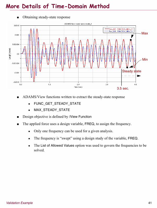
� Obtaining steady-state response
� ADAMS/View functions written to extract the steady-state response
� FUNC_GET_STEADY_STATE
� MAX_STEADY_STATE
� Design objective is defined by /View Function
� The applied force uses a design variable, FREQ, to assign the frequency.
� Only one frequency can be used for a given analysis.
� The frequency is �swept� using a design study of the variable, FREQ.
� The List of Allowed Values option was used to govern the frequencies to be solved.
Steady state
3.5 sec.
Max
Min
More Details of Time-Domain Method

42 Validation Example
� Plotting
� System modes
� Frequency response
� Magnitude
� Phase
� Power spectral density (PSD)
� Modal coordinates
� Modal participation
� Animation
� Normal-mode animation
� Forced-vibration animation
� Modal info tables
� Modal coordinates
� Modal participation
� Modal energy
Each can be saved to a file (HTML or text).�
� Briefly demonstrate most of the above features using the two-DOF model from this workshop.
Post-Processing

Validation Example 43
This workshop takes about one hour to complete.
Problem statementUse time domain simulation results to validate the accuracy of frequency domain solutions.
In this workshop, you will run a series of simulations in the time domain and compare the steady state vibratory behavior of the model with the output from a frequency domain simulation. The process is as follows:
� Excite the system at a given frequency in time domain.
� Once the system has achieved steady state, compute the system response by taking the average of the minimum and maximum response peaks.
This gives the steady state response (magnitude) of the system at a given frequency.
� Perform frequency response in ADAMS/Vibration using a swept sine actuator.
� Compare vibration frequency response with steady state response.
This process is a way to validate your ADAMS/Vibration results, while appreciating the speed advantages of using frequency domain solution.
XII III
III
IVVVIVII
XXI
VIII
IX
Workshop 2�Validation Example

44 Validation Example
Model description
� This model is similar to the one used in Workshop 1—Introduction on page 26.
� The masses of the blocks are equal (that is, block1_mass=block2_mass).
� Gravity is turned off.
Getting startedFirst you will start ADAMS/View and import the model.
To import the model:
1 Start ADAMS/View from the mod_02_validation directory.
2 Import the model, valid_start.cmd.
This command file includes:
� A 2-DOF spring mass model
� A function to compute steady-state time domain response
� A design objective that uses this function
Exciting the system in the time domainIn the last workshop, you vibrated (excited) the system in the frequency domain with an actuator. To perform the validation experiment, you will use a single-component force (SFORCE) to excite the system in the time domain. You will create a design variable that defines the excitation force that will drive the system at specific discrete frequencies.
To create a design variable to define excitation frequencies:
1 From the Build menu, point to Design Variable, and then select New.
Workshop 2�Validation Example...

Validation Example 45
2 Complete the Create Design Variable dialog box as follows:
3 Select OK.
To create an SFORCE to excite mass M2 at a frequency of FREQ:
1 From the Main Toolbox, within the Create Forces toolstack, select the Applied Force: Force
(Single Component) icon .
2 Set Run-Time Direction to Space Fixed.
3 Set Construction to Pick Feature.
4 Set Characteristic to Custom.
5 Follow the prompts in the Status Bar, selecting the following:
� M2 as the body
� PT_3 as the point of application (that is, the center of M2)
� cm.Y as the vertical direction vector.
Tip: If you're having trouble selecting the y-axis, right-click PT_3.
The Modify Force dialog box appears.
6 In the Function text box, enter the following function expression:
1.0*sin(2*PI*.model_1.FREQ*time)
This function uses the FREQ design variable you created earlier. The SFORCE function will impart a 1-Newton sinusoidal force at the frequency, FREQ.
7 Select OK.
The five frequencies at which you’ll be exciting mass M2.
� Name: .model_1.FREQ
� Standard value: 4.0
� Value Range by: Absolute Min and Max Values
� Min. Value: 4.0
� Max. Value: 8.0
� List of allowed values:4.0, 5.0, 5.5, 6.0, 7.0
Workshop 2�Validation Example...

46 Validation Example
Performing a design evaluationNext, you will perform a design evaluation using the existing objective, FREQ_RESP.
Understanding details of the functions
In each trial of the design study, the excitation frequency, FREQ, will drive the system at a different frequency (4 Hz, 5 Hz, and so on). You want to obtain the frequency response magnitude (at steady state) for each of these trials. In this workshop, you will use two ADAMS/View functions to compute the system response by taking the average of the minimum and maximum response peaks:
� FUNC_GET_STEADY_STATE: This function extracts the steady state value from the measure FUNCTION_MEA_DY. It is assumed that steady state has been reached at 3.5 seconds so it takes all the values of the measure corresponding to times equal or greater than 3.5 seconds. This function uses matrix indexing and expressions. You can think of it having the simplified form:
FUNCTION_MEA_DY.Q.values[index at 3.5 seconds : index at end time]
� MAX_STEADY_STATE: This function computes the amplitude of FUNCTION_MEA_DY at steady state by extracting the MAX and MIN values and computing the average of these values. It calls the FUNC_GET_STEADY_STATE function so that it only operates on steady state values. You can think of it having the following simplified form:
(MAX (FUNC_GET_STEADY_STATE)-MIN (FUNC_GET_STEADY_STATE)) / 2.0
The design objective FREQ_RESP simply calls the function MAX_STEADY_STATE to calculate the magnitude of the vibratory response at steady state. The design objective FREQ_RESP simply calls the function MAX_STEADY_STATE to calculate the magnitude of the vibratory response at steady state; let's take a closer look at it.
To see how the design objective has been defined:
1 From the Simulate menu, point to Design Objective, and then select Modify.
2 From the Database Navigator, double-click the model name, and then select FREQ_RESP.
3 Review the contents of the Modify Design Objective dialog box, then close it by selecting Cancel.
The model is ready to be solved in the time domain, but before you do that, you should adjust a few settings in the interface.
Workshop 2�Validation Example...

Validation Example 47
To prepare simulation settings for design evaluation:
1 To avoid update of graphics during simulation, perform the following:
� From the Settings menu, point to Solver, and then select Display.
� Set Show Messages to Yes.
� Set Update Graphics to Never.
Do not close the dialog box.
2 To generate screen output so you can conveniently monitor simulation progress, use the external solver, do the following:
� Set Category to Executable.
� Set Executable to External.
3 To store the individual and multi-run simulation results in the database, perform the following:
� Set Category to Output.
� Select More.
� Set Output Category to Database Storage.
� Under Individual Simulations, set Save Analysis to Yes, and set Prefix to Run.
� Under Multi-Run Simulations, set Save Analysis to Yes, and set Prefix to Multi_Run.
4 Select Close.
5 To save the individual simulation on disk:
� From the Settings menu, point to Solver, and then select Output.
� Set Output Category to Files.
� Set Save Files to Yes.
� Select Close.
6 To direct the files to another directory:
� From the File menu, point to Select Directory, and then select results_dir.
� Select OK.
Workshop 2�Validation Example...

48 Validation Example
To perform the design evaluation:
1 From the Simulate menu, select Design Evaluation.
2 Prepare the design study to study objective FREQ_RESP by completing the Design Evaluation Tools dialog box as follows:
� Model: .model_1
� Simulation Script: SIM_SCRIPT_ACF
� Study a Objective: FREQ_RESP
� Select Design Study
� Design Variable: FREQ
The SIM_SCRIPT_ACF script uses the following series of ADAMS/Solver commands:
Notice that after 3 seconds of simulation, the integrator error is tightened and the output step size is reduced by a factor of 5. This is done to distribute enough points evenly over the peaks and valleys of the output signal so that the maximum and minimum values are captured correctly.
3 Select Start.
The five design evaluations will take a while. When they�re done, ADAMS/Vibration will write a table of results to the information window. In addition, ADAMS/Vibration will display the following information box:
SIMULATE/STATICINTEGRATOR/SI2, ERROR=1E-4, HMAX=1e-4SIMULATE/TRANSIENT, END=3.0, DTOUT=0.005
INTEGRATOR/SI2, ERROR=1E-5, HMAX=1e-4SIMULATE/TRANSIENT, END=4.0, DTOUT=0.001
Workshop 2�Validation Example...

Validation Example 49
4 Close the Information box.
5 Close the Info window.
6 Select the Create Tabular Report of Results tool. Complete the dialog box as follows:
� Result Set: Last_Multi.Design_Study_Results
� File Name: DS_table.txt
7 Select OK.
8 Inspect the results in the Info window, and then close the window.
9 Store the time-domain simulations by saving the database:
� From the File menu, select Save Database.
Plotting individual runs of the design study
To plot the design study:
1 Open ADAMS/PostProcessor by pressing F8.
2 Set Source to Measures.
3 From the Simulation list, hold down the Ctrl key while selecting Run_001 and Run_005.
Hint: Don�t select Last_Run.
4 From the Measure list, select FUNC_MEA_DY.
This will select the vertical displacement of mass M1.cm relative to ground.
Workshop 2�Validation Example...

50 Validation Example
5 Select Add Curves.
The plot should look like the following. You may have to move the legend.
After the initial transient has died out, the vibration reaches a steady state solution. The amplitude at steady state is the vibratory response of the system.
6 Use the Surf option and review the vibratory characteristics of the other runs named Run_*.
7 Return to ADAMS/View by pressing F8.
Steady state
3.5 sec.
Workshop 2�Validation Example...

Validation Example 51
Analyzing frequency response with ADAMS/VibrationYou already generated the time-domain results needed to validate ADAMS/Vibration. Now you will perform the frequency response analysis in the frequency domain. In this section you will:
� Load the ADAMS/Vibration plugin
� Create an input channel and actuator
� Create an output channel
� Define and perform the vibration analysis
To load the ADAMS/Vibration plugin:
� From the Tools menu, point to Plugins, point to Vibration, and then select Load.
To create the input channel and actuator:
1 From the Build menu, point to ADAMS/Vibration, point to Input Channel, and then select New.
The Create Vibration Input Channel dialog box appears.
2 In the Input Channel Name text box, enter .model_1.Input_Channel_1.
3 Right-click the Input Marker text box, point to Marker, and then select Browse.
The Database Navigator appears.
4 Double-click M2.cm.
ADAMS/Vibration inserts this marker into the Input Marker text box.
5 Select Translational.
6 Set the Force Direction to Global Y.
7 Select Actuator Parameters.
8 Select Swept Sine.
9 In the Force Magnitude text box, enter 1.0.
10 In the Phase Angle (deg) text box, enter 0.0.
11 Select OK.
Workshop 2�Validation Example...

52 Validation Example
To create the output channel:
1 Create an output channel for M1.cm that measures Global Y displacement.
Tip: This output channel is identical to the one you created in Creating an output channel on page 31.
To define and perform the vibration analysis:
1 From the Simulate menu, point to Interactive Controls.
The Simulation Control dialog box appears.
2 Select the Vibration Analysis tool .
The Perform Vibration Analysis dialog box appears. Complete the dialog box as shown below:
Workshop 2�Validation Example...

Validation Example 53
3 Select OK.
ADAMS/Vibration performs a forced-vibration analysis.
Note: Because we�re still using the standalone Solver for the vibration analysis, a benign warning will be issued to the message window when ADAMS/vibration reads in the analysis files.
WARNING: The request file contains no time dependent data.
Ignore the message and close the message window.
4 After the simulation has finished, close the Information window.
Plotting vibration analysis resultsNext you will plot the vibration analysis results with the design study results.
To plot the results:
1 Open ADAMS/PostProcessor by pressing F8.
2 Select the New Page tool .
3 Plot the magnitude frequency response for the vibration analysis like you did in Plotting frequency response on page 33.
4 From the Source list, select Result Sets.
5 From the Simulation list, select Multi_Run_001.
6 From the Result Set list, select Design_Study_Results.
7 From the Component list, select FREQ_RESP.
8 Set Independent Axis to Data.
The Independent Axis Browser displays.
9 In the Independent Axis Browser, set Component to FREQ.
10 Select OK.
11 Select Add Curves.
The design study results (in dashed blue) are plotted on top of the vibration results (in solid red).
Workshop 2�Validation Example...

54 Validation Example
Next, you will change the curve for the design study results so that it has symbols instead of a line.
To modify the plot layout:
1 Select the design study results curve, either by left-clicking it, or by navigating through the treeview.
2 In the property editor, perform the following:
� Set Symbol to @.
� Set Line Style to none.
3 In the treeview, select haxis (the horizontal axis).
4 In the Scale list, select Linear.
5 In the treeview, select vaxis (the vertical axis).
6 In the property editor, select the Labels tab.
7 In the Label text box, enter Magnitude (dB).
8 In the treeview, select legend_object (the legend).
9 From the Placement list, select Bottom Left.
10 Select one of the plot's internal grid lines.
11 In the Title text box, enter Validation of Frequency Response - Magnitude. To do this, you may have to clear the selection of Auto Title.
12 In the Subtitle text box, enter Results Comparison: Time Domain versus Frequency Domain. To do this, you may have to clear the selection of Auto Subtitle.
13 In the property editor, select the 2nd Grid tab.
Tip: To find the tab, use the arrow keys in the property editor.
Workshop 2�Validation Example...

Validation Example 55
14 In the Y text box, enter 2.
The modified plot appears as shown below:
The results of the five time-domain solutions have validated the single ADAMS/Vibration analysis.
15 How many frequencies were studied using the Design Study? _____________
16 How many frequencies were solved using ADAMS/Vibration? ______________
17 Has the frequency-domain solution solved for more frequencies in less time? __________Yes __________ No
Wrap-up1 Exit ADAMS/PostProcessor and return to the modeling window.
2 Exit ADAMS/View.
Workshop 2�Validation Example...

56 Validation Example
Workshop 2�Validation Example...

57
3 POWER SPECTRAL DENSITY (PSD)
Determine the power spectral density (PSD) output at the driver's seat in a conceptual vehicle model for a given road input PSD.
What�s in this module:� PSD—What is it?, 58
� PSD Actuator, 59
� Workshop 3—Power Spectral Density (PSD) Input, 60

58 Power Spectral Density (PSD)
� Power spectral density is the amount of power per unit (density) of frequency (spectral) as a function of the frequency.
� The power spectral density describes how the power (or variance) of a time series is distributed over a frequency range.
� PSD can also be understood as a measure of the intensity in the frequency domain.
� Mathematically, it is defined as the Fourier transform of the auto correlation sequence of the time series. An equivalent definition of PSD is the squared modulus of the Fourier transform of the time series, scaled by a proper constant term.
� Being power per unit of frequency, the dimensions are those of power divided by Hertz.
PSD�What is it?

Power Spectral Density (PSD) 59
� The PSD vibration actuator is defined using a spline function.
� Either a force PSD or a displacement PSD can be specified.
� For the displacement PSD, a corresponding stiffness must be specified.
� Notes:�
� It is assumed that the PSD inputs applied to the linear model are independent of one another. In other words, they are not correlated.
� You cannot combine vibration actuators of the non-PSD-type with PSD-type vibration actuators in the same vibration analysis.
� A feature for cross-correlation of PSD input will be available in version 13.0.
PSD Actuator

60 Power Spectral Density (PSD)
This workshop takes about 45 minutes to complete.
Problem statementDetermine the power spectral density (PSD) output at the driver's seat in a conceptual vehicle model for a given road input PSD.
In this workshop you will determine the effect that road vibration has on a passenger. You will learn how to define a PSD vibration actuator.
You can define four kinds of actuators in ADAMS/Vibration:
� Swept Sine
� Rotating Mass
� PSD
� User
After finishing all of the workshops, you will know how to define all of the actuator types. You should already be comfortable with the swept sine actuator, since you used it in the last two workshops. In this workshop you will focus on the PSD actuator. In Workshop 4—User-Specified Vibration Actuators on page 79, you will learn about the user-defined actuator. Finally, you will use the rotating mass type in Workshop 5—Rotating Mass Vibration Actuator on page 97.
XII III
III
IVVVIVII
XXI
VIII
IX
Workshop 3�Power Spectral Density (PSD) Input

Power Spectral Density (PSD) 61
Model description� The model is a conceptual vehicle model with passenger, and 16 DOF.
� It has six moving parts (four wheels, chassis, and seat).
� The seat part (and passenger) is a block mounted to the vehicle with a bushing.
� Each wheel is connected to the chassis with a translational joint and spring-damper force.
� Bushing forces act between the wheels and ground.
� Stiffness and damping coefficients throughout the model have been parameterized with design variables; some geometric and mass characteristics have also been parameterized.
Workshop 3�Power Spectral Density (PSD) Input...

62 Power Spectral Density (PSD)
Category: Design Variable: Description:
Damping for spring dampers between wheel and chassis
flwhdampfrwhdamprlwhdamprrwhdamp
Front left wheel damping coefficientFront right wheel damping coefficientRear left wheel damping coefficientRear right wheel damping coefficient
Stiffness for spring dampers between wheel and chassis
flwhstifffrwhstiffrlwhstiffrrwhstiff
Front left wheel stiffness coefficientFront right wheel stiffness coefficientRear left wheel stiffness coefficientRear right wheel stiffness coefficient
Stiffness and damping for seat bushing
seat_stiffseat_dampseat_t_stiffseat_t_damp
Translational stiffness of seat_chassis_bushTranslational damping of seat_chassis_bushTorsional stiffness of seat_chassis_bushTorsional damping of seat_chassis_bush
Stiffness and damping for bushings between wheel and ground
k_x, k_y, k_z
c_x, c_y, c_z
tk_x, tk_y, tk_z
tc_x, tc_y, tc_z
Translational stiffness coefficients for bush-ings: fl_bush, fr_bush, rl_bush, rr_bush.Translational damping coefficients for bush-ings: fl_bush, fr_bush, rl_bush, rr_bush.Torsional stiffness coefficients for bushings: fl_bush, fr_bush, rl_bush, rr_bush.Torsional damping coefficients for bushings: fl_bush, fr_bush, rl_bush, rr_bush.
Geometric wheelbasefront_trackrear_track
Distance between front and rear wheel axlesDistance between front wheel centersDistance between rear wheel centers
Mass passenger_mass
Mass of seat and passenger combined.
Mass/Geometric weight_dist Weight distribution expressed as a fraction (such as 0.51); this variable will shift the chassis geometry fore-aft.
Workshop 3�Power Spectral Density (PSD) Input...

Power Spectral Density (PSD) 63
Getting startedFirst, you will import the model and load the ADAMS/Vibration plugin.
To import the model and load the plugin:
1 Start ADAMS/View from the working directory exercise_dir/mod_03_psd (where exercise_dir is the directory where your exercise files are installed).
2 Import the model car_start.cmd.
3 From the Tools menu, point to Plugins, point to Vibration, and then select Load.
Creating input channelsNext, you will create input channels to apply vibration forces to the front wheels. You will also create a vibration actuator for PSD. The displacement PSD data is given in the form of a spline. Before creating the vibration input and output channels, let's take a look at the input spline that you will be using, SPLINE_1.
To view SPLINE_1 as a plot:
1 From the Build menu, point to Data Elements, point to Spline, and then select Modify.
2 From the Database Navigator, double-click the model name and select SPLINE_1.
The Modify spline dialog box appears.
Workshop 3�Power Spectral Density (PSD) Input...

64 Power Spectral Density (PSD)
3 Set View As to Plot.
The plot displays as shown below:
This is the PSD data that will be applied to the front wheels of the model. The frequency range of this spectrum goes from 0.1 to 10 hertz.
4 Close the Modify spline dialog box.
Creating the input channels and PSD actuatorNext, you will create an input channel at the front left wheel, flwheel, and assign a displacement PSD actuator. Then you will create a similar input channel at the front right wheel, frwheel, reusing the same actuator as used at the left wheel.
To create the input channels and PSD actuator:
1 From the Build menu, point to ADAMS/Vibration, point to Input Channel, and then select New.
The Create Vibration Input Channel dialog box appears.
2 In the Input Channel Name text box, enter .automobile.Input_Channel_FL.
Workshop 3�Power Spectral Density (PSD) Input...

Power Spectral Density (PSD) 65
3 Right-click in the Input Marker text box, point to Marker, and then select Browse.
4 Double-click flwheel.cm.
ADAMS/Vibration inserts this marker into the Input Marker text box.
5 Select Translational.
6 Set Force Direction to Global Z.
7 Select Actuator Parameters.
8 Select PSD.
9 Select Displacement.
10 In the Spline Name text box, browse to SPLINE_1.
11 Set Interpolation Type to akima.
12 In the Stiffness Coefficient text box, enter 1000.
13 Select Apply.
14 Create the input channel for the front right wheel, frwheel:
� In the Input Channel Name text box, enter .automobile.Input_Channel_FR.
� Right-click the Input Marker text box, point to Marker, and then select Browse.
� Double-click frwheel.cm.
ADAMS/Vibration inserts this marker into the Input Marker text box.
� From the Actuator Parameters list, select Use Existing Actuator.
� Right-click the Vibration Actuator Name text box, point to Vibration_Actuator, point to Guesses, and then select Vibration_Actuator_1.
15 Select OK.
Now you�re ready to create the output channels.
Workshop 3�Power Spectral Density (PSD) Input...

66 Power Spectral Density (PSD)
Creating output channelsHere you create output channels to measure displacement and velocity at the driver's seat.
To create the output channels:
1 Create an output channel for measuring displacement:
2 Select Apply.
3 Create another output channel to measure velocity:
4 Select OK.
Workshop 3�Power Spectral Density (PSD) Input...

Power Spectral Density (PSD) 67
Performing vibration analysisNext, you perform a vibration analysis using the input and output channels you just created.
To perform a vibration analysis:
1 From the Simulate menu, point to ADAMS/Vibration, and then select Vibration Analysis.
2 Complete the dialog box as shown next:
Tip: If you double-click the blank Input Channels text box, the Database Navigator appears allowing you to select both channels at once.
3 Select OK.
Make sure you leave this unchecked
Workshop 3�Power Spectral Density (PSD) Input...

68 Power Spectral Density (PSD)
Plotting output PSDNow you plot the output PSD in ADAMS/PostProcessor. You will observe the resonance peaks due to the input vibration and the model parameters.
To plot PSD output:
1 Open ADAMS/PostProcessor.
2 Right-click the viewport and select Load Plot.
3 Set Source to PSD.
4 From the Output Channels list, select seat_displacement and seat_velocity by holding down the Ctrl key while selecting.
5 Select Add Curves.
ADAMS/PostProcessor generates the Vibration PSD plot, showing one curve for each output channel. Notice that both curves are similar in shape.
6 Delete the curve representing the velocity.
Hint: Right-click the dashed blue curve, and then select Delete.
Workshop 3�Power Spectral Density (PSD) Input...

Power Spectral Density (PSD) 69
7 Add symbols to the red displacement curve so you can see the discrete output data:
� Select the curve representing the displacement.
� In the property editor, from the Symbol list, select o.
� Unselect the curve by clearing the select list.
Tip: Click the Select arrow to clear the list.8 Change the horizontal axis to a linear scale so you can better visualize the curve data:
� From the treeview select haxis.
� In the property editor, from the Scale list, select Linear.
� Clear the select list.
Review the Output PSD curve and then answer the following questions:
9 Does the output resolution seem sufficient enough to capture the resonance peaks?
Yes _____ No _____
10 Why doesn't the lower bound of your PSD output plot extend leftward to 0.10 Hz like you requested in the vibration analysis specification in step 2 on page 67?
_____________________________________________________________________
______________________________________________________________________
11 Earlier in the workshop, you learned that the PSD input spline, SPLINE_1, had a range of 0.1 - 10 Hz. Suppose you had set the Vibration Analysis end frequency to 100 Hz; what do you think the vibration solver would do?�
_________________________________________________________________
12 Use the F8 key to close the plot window and return to the modeling view.
� CR32306 has been logged to address the issue of the analysis frequency range not being honored.
Workshop 3�Power Spectral Density (PSD) Input...

70 Power Spectral Density (PSD)
Running vibration analysis againHere you'll rerun the vibration analysis with higher output resolution to better identify the resonance peaks. You can reuse the existing state matrices, since neither the model nor the inputs/outputs changed.
To run a vibration analysis:
1 From the Simulate menu, point to ADAMS/Vibration, and then select Vibration Analysis.
2 Select Vibration Analysis.
3 Right-click the Vibration Analysis text box, point to Vibration_Analysis, point to Guesses, and then select VibrationAnalysis_PSD.
Notice how ADAMS/Vibration updates the Perform Vibration Analysis dialog box with the analysis specifications you used before.
4 Change the frequency range and steps as follows:
� Begin: 0.1
� End: 10.0
� Steps: 500
5 Select Reuse Existing State Matrices.
Notice that many parts of the dialog box are greyed out. This is to ensure that you don�t accidently change any of the inputs and outputs.
6 Select OK.
Plotting new outputHere you replot the output PSD so you can see the improved resolution of the resonance peaks.
To plot the output:
1 Launch ADAMS/PostProcessor.
2 Select the Reload Simulations tool .
Workshop 3�Power Spectral Density (PSD) Input...

Power Spectral Density (PSD) 71
ADAMS/PostProcessor plots the new simulation results, demonstrating the increased resolution.
3 Note significant peaks and valleys and write their frequencies here:
Peaks _______ _______ _______ _______
Valleys _______ _______ _______ _______
Tip: Use the Zoom tool .
You will animate the results at these frequencies later in the workshop.
4 Return to the modeling window.
Changing parametersNow, you change the damping properties of spring dampers and run another vibration analysis to see how the vibration response changes. You create an analysis by importing the specifications from the last simulation.
The vehicle model you've solved so far had what you might consider �brand new� dampers, with each damping coefficient being equal and at a nominal design value. Now suppose that over the life of the vehicle, the dampers had worn so that they are no longer equal from wheel-to-wheel, and now supply less damping altogether. To reflect this scenario by importing a command file, you update the damping parameters.
Workshop 3�Power Spectral Density (PSD) Input...

72 Power Spectral Density (PSD)
To change the damping parameters:
� Using the F2 key, import the file uneven_damper_wear.cmd in the damper_wear subdirectory.
This file automatically sets the design variables for the �worn-out� condition as follows:
To run a vibration analysis:
1 From the Simulate menu, point to ADAMS/Vibration, and then select Vibration Analysis.
2 Select New Vibration Analysis.
3 Clear the New Vibration Analysis text box, and enter Uneven_Damper_Wear.
4 Select Import Settings from Existing Vibration Analysis, and when the Database Navigator opens, select VibrationAnalysis_PSD.
Notice that ADAMS/Vibration updates the Perform Vibration Analysis dialog box with the analysis specifications you used before.
5 Select OK.
Design variable: Damping coefficient:
flwhdamp 1e-3
frwhdamp 0.5
rlwhdamp 0.8
rrwhdamp 1.0
Workshop 3�Power Spectral Density (PSD) Input...

Power Spectral Density (PSD) 73
Plotting new outputNow you can compare the two damper conditions by plotting the output.
To plot the output:
1 In ADAMS/PostProcessor, create a new page.
2 Set Source to PSD.
3 From the Vibration Analysis list, select both VibrationAnalysis_PSD and Uneven_Damper_Wear.
4 From the Output Channels list, select seat_displacement.
5 Select Add Curves.
6 From the treeview, select haxis.
7 In the property editor, from the Scale list, select Linear.
8 Clear the select list.
9 Use the treeview and property editor to change the dashed-blue curve to a solid line.
The resonant peaks have increased in magnitude due to the reduction of damping resulting from the worn-out dampers.
Workshop 3�Power Spectral Density (PSD) Input...

74 Power Spectral Density (PSD)
Understanding vibrationFinally, you will use the Forced Vibration Animation tool to understand how the conceptual vehicle vibrates when excited at different frequencies.
To animate the vibration:
1 Create a new page.
2 Right-click the viewport and select Load Vibration Animation.
3 In the Database Navigator, select Uneven_Damper_Wear.
4 View the model from the right side by using the Shift-R keyboard shortcut.
5 In the dashboard, select Automatically set time fields for one cycle.
6 In the text box beneath the Frequency slider, double-click the existing value and enter 1.54 to update the frequency.
7 In the Maximum Translation text box, enter 50.
8 To animate the vibration, select the Play tool.
Notice that the wheels are vibrating out of phase because their damping rates are unequal.
9 Repeat the above steps to animate the response for the VibrationAnalysis_PSD results.
10 How are the wheels vibrating at 1.54 Hertz for the VibrationAnalysis_PSD analysis?
____ In phase
____ Out of phase
Explain why: ____________________________________________________________
11 Animate the forced vibration results for the other frequencies that you recorded earlier, on page 71.
Wrap up1 Close ADAMS/PostProcessor and return to the modeling window.
2 Save your database.
3 Exit ADAMS/View.
Workshop 3�Power Spectral Density (PSD) Input...

Power Spectral Density (PSD) 75
Optional tasks1 Perform a design study of weight_dist to see how the vehicle�s fore/aft weight distribution
influences the resonant frequencies.
a Import the file misc/prep_for_design_study.cmd. This file will build the simulation script and create an objective that calculates the peak magnitude across the frequency spectrum.
b Run the design study with the following parameters:
� model_name: .automobile
� sim_script_name: Design_Study_Script
� objective_names: OBJ_MAG
� variable_name: weight_dist
� number_of_levels: 5
c Plot the PSD output for the individual runs, using a linear frequency scale.
d Animate the vibration at frequencies of interest.
Workshop 3�Power Spectral Density (PSD) Input...

76 Power Spectral Density (PSD)
Workshop 3�Power Spectral Density (PSD) Input...

77
4 USER-DEFINED INPUT
Vibrate the conceptual vehicle by applying a general function of frequency through a vibration actuator.
What�s in this module:� Overview, 78
� Workshop 4—User-Specified Vibration Actuators, 79

78 User-Defined Input
� Any user function of the independent variable, omega, can be specified in the ADAMS/View Function Builder:
f(ω ) = g(ω )
where:
� ω is the frequency
� g(ω ) is the general function of omega �
�
� There are some limitations to using the SPLINE function in your user expression. Currently, no interpo-lation is being done, so you will have to interpolate the data to align with the outputs.
� You can think of the user function as a way of directly controlling the amplitude of a swept sine with yourown function.
Amplitude determinedby user function
Frequency increasingover interval
Overview

User-Defined Input 79
This workshop takes about 30 minutes to complete.
Problem statementVibrate the conceptual vehicle by applying a general function of frequency through a vibration actuator.
In this workshop you will see how you can write your own frequency-based function to vibrate a model at its input channels. You will learn to modify an existing vibration model to suit a different vibratory condition. In this example, you will take the conceptual vehicle model from the last workshop and change its vibration actuator force from PSD to a user-written function. You will also learn to plot system modes, modal participation, and modal coordinates.
XII III
III
IVVVIVII
XXI
VIII
IX
Workshop 4�User-Specified Vibration Actuators

80 User-Defined Input
Model descriptionThe model is the same conceptual vehicle model used in Workshop 3—Power Spectral Density (PSD) Input on page 60. The wheel-to-chassis dampers have equal properties that represent the brand-new (or unworn) condition.
Getting startedFirst, you import the model and load the ADAMS/Vibration plugin.
To import model and load the plugin:
1 Start ADAMS/View from the working directory exercise_dir/mod_04_userfunc (where exercise_dir is the directory where your exercise files are installed).
2 Import the model user_start.cmd.
3 Select the Build menu and look at the last submenu.
4 Do you see ADAMS/Vibration listed? ________Yes _________No
Here, you don't need to load the vibration plugin because the command file automatically loaded the plugin for you. Let's see how that was accomplished.
5 Using a text editor (such as Notepad), open the command file user_start.cmd.
6 Using the text editor's find (or search) tool, search for the parameter plugin_name.
This will take you to the section of the command file that loads the plugin for you, as shown here:
You can see that the command file is issuing a straightforward command to load the ADAMS/Vibration plugin from the .MDI.plugins library. When you load the plugin yourself (through the Tools -> Plugins menu), it executes the same command. You can learn more about your models and the commands used to build them by reviewing the contents of your command files.
7 Close your text editor without saving.
!--------------------------- Plugins used by Model ----------------------------!
!
!
plugin load &
plugin_name = .MDI.plugins.vibration
Workshop 4�User-Specified Vibration Actuators...

User-Defined Input 81
Creating input channelsNext, you modify the existing left and right input channels so that they use a user-defined vibration actuator function representing exponential frequency decay.
1 From the Build menu, point to ADAMS/Vibration, point to Input Channel, and then select Modify.
2 When the Database Navigator opens, double-click the model name and select Input_Channel_FL.
The Modify Vibration Input Channel dialog box appears.
3 Select User.
4 In the f(omega) text box, enter the function expression (1000*exp(-omega)).
Here, omega represents the frequency in frequency-domain models. It is analogous to the time function that you are accustomed to using in your time-domain models.�
5 In the Phase Angle (deg) text box, enter 0.
6 Select Apply.
You have updated the left wheel's input channel and vibration actuator. Now you should check the input channel at the right wheel to see what it is set to.
7 Right-click the Input Channel Name text box, point to Input Channel, point to Guesses, and then select Input_Channel_FR.
The dialog box updates with the specifications for the input channel at the right wheel.
� The input marker field now contains .automobile.frwheel.cm, the center of mass marker for the right wheel.
� The input channel is a translational force, operating in the global z direction.
Now take a look at the actuator parameters. Notice that they already contain the User setting, as well as the function you defined for the left wheel, even though you haven�t modified the right wheel yet. This is because the second input channel that you created in Workshop 3—Power Spectral Density (PSD) Input used an existing actuator that was created with the first input channel. In doing this, you built two input channels but only a single vibration actuator, which is being used by both input channels.
� CR32372 has been logged to improve documentation of the omega function.
Workshop 4�User-Specified Vibration Actuators...

82 User-Defined Input
8 Select Cancel.
Another way to see how input channels have been defined is to look at them in the Information window.
Getting information about a model's input channelsHere you learn how to obtain modeling information about the input channels. You use the Select List Manager to find all the input channels in the model, put them on the select list, and then get information about them. You will also further investigate modeling details about the vibration actuator that is associated with the input channels.
To view information on the input channels:
1 From the Edit menu, select Select List.
The Select List Manager dialog box appears.
2 Set the option menu next to the Type Filter text box to Browse.
3 In the Database Types dialog box that opens, double-click Input_Channel.
4 Select the Add button at the bottom.
The Select List Manager's objects text box updates with the two input channels in the model.
Workshop 4�User-Specified Vibration Actuators...
User-Defined Input 83
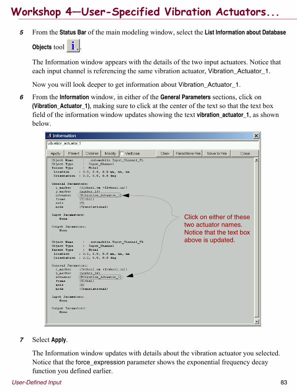
5 From the Status Bar of the main modeling window, select the List Information about Database
Objects tool .
The Information window appears with the details of the two input actuators. Notice that each input channel is referencing the same vibration actuator, Vibration_Actuator_1.
Now you will look deeper to get information about Vibration_Actuator_1.
6 From the Information window, in either of the General Parameters sections, click on (Vibration_Actuator_1), making sure to click at the center of the text so that the text box field of the information window updates showing the text vibration_actuator_1, as shown below.
7 Select Apply.
The Information window updates with details about the vibration actuator you selected. Notice that the force_expression parameter shows the exponential frequency decay function you defined earlier.
Click on either of these two actuator names. Notice that the text box above is updated.
Workshop 4�User-Specified Vibration Actuators...

84 User-Defined Input
8 To empty the contents of the information window, select Clear.
9 To close the information window, select Close.
10 To clear the Select List, select Clear All.
11 To close the Select List Manager, select Close.
Redefining an existing vibration analysisHere you define the analysis by importing the settings from the existing PSD specification, and then perform the vibration analysis.
To run the vibration analysis:
1 From the Simulate menu, point to ADAMS/Vibration, and then select Vibration Analysis.
2 In the New Vibration Analysis text box, enter VibrationAnalysis_User.
3 Select Import Settings from Existing Vibration Analysis, and when the Database Navigator appears, double-click VibrationAnalysis_PSD.
The Perform Vibration Analysis dialog box updates with the analysis specifications you used in the last workshop.
4 Select Logarithmic Spacing of Steps.
5 Leave the Begin and End times as-is (0.1 and 10.0, respectively).
6 In the Steps text box, reduce the data resolution by changing the value from 500 to 50.
7 Select OK.
When the vibration analysis is finished, the dialog box will close by itself.
Plotting Vibration Analysis OutputHere you will plot system modes, modal participation, and modal coordinates.
To plot system modes:
1 Launch ADAMS/PostProcessor.
2 Set Source to System Modes.
3 From the Eigen list, select EIGEN_1.
Workshop 4�User-Specified Vibration Actuators...

User-Defined Input 85
4 Select Add Scatters.
ADAMS/PostProcessor plots the real and imaginary parts of the eigenvalue solution. Here you can see that the model is stable because the system modes do not lie in the positive real quadrants.
5 Right-click the Page Layout tool, and select the 2 Views, over & under tool .
6 Right-click the viewport and select Load Vibration Animation.
7 From the Database Navigator, double-click the model name and then double-click VibrationAnalysis_User.
8 In the dashboard, select Table of Eigenvalues.
The Information window displays a table containing the eigenvalues.
Note: If your Information window displays other information leftover from earlier steps, clear the window and repeat step 8.
9 In the Information window, select Save to File.
10 Save the file as eigenvalues.txt.�
11 Close the Information window.
The table has been saved to disk. Now you will import that data into the animation window so that it will be displayed below the scatter plot.
12 Right-click the animation window and select Load Report.
13 From the Select File browser, select eigenvalues.txt.
14 If a warning dialog box appears, select OK so that the animation is deleted.
The eigenvalue table displays in the report window. Now you will reduce the font size so that you can see more of the data in the window.
15 Select the report window by clicking in it.
16 In the property editor, enter 7 in the Font Size text box.
17 To hide the dashboard, select the Toggle Dashboard Visibility icon .
� Some students my be confused during the saving process because the button says Open, when you'd thinkit should say Save.
Workshop 4�User-Specified Vibration Actuators...

86 User-Defined Input
You should see something similar to what is shown below.
Plotting modal participationHere you will learn to plot modal participation graphically. This will help you understand which of the system�s eigenmodes are active (or participating) when the system is forced at a given frequency.
To plot modal participation:
1 Perform the following:
� Select the New Page tool.
� Right-click the Page Layout tool, and then select the Page Layout: 1 Views tool .
� To redisplay the dashboard, select the Toggle Dashboard Visibility icon.
� Right-click the viewport and select Load Plot.
Workshop 4�User-Specified Vibration Actuators...

User-Defined Input 87
2 Set Source to Modal Participation.
3 Select Surf.
4 From the Input Channels list, select Input_Channel_FL.
5 From the Output Channels list, select seat_velocity.
6 From the Modes list, select modes 5 through 8.
7 Select Magnitude.
ADAMS/PostProcessor plots the participation of modes 5 through 8. Here you can see that mode 7 makes little contribution across the entire frequency spectrum, whereas mode 6 participates across several frequencies, coming to a significant magnitude peak between 5.0 to 6.0 hertz.
8 If you used the Plot Tracking tool, clear its selection.
9 From the Modes list, select mode 10.
Notice that this mode participates in a different manner.
10 Use the up and down arrows on your keyboard to surf (or scroll) through the other modes in the Modes list, inspecting their modal participation.
Be sure to take note of the values on the vertical axis as you review the modes; they will update as you are surfing. You may also notice the curves to be lacking smoothness; this is due in part to the coarseness of the output resolution (only 50 outputs, logarithmically spaced). We have chosen to keep the output to a minimum so that the plots in the next section of the workshop are easier to inspect.
Workshop 4�User-Specified Vibration Actuators...

88 User-Defined Input
Plotting modal coordinatesHere you access modal coordinates results in a graphical way. Later on, in Workshop 5—Rotating Mass Vibration Actuator, you'll learn how to access the same data in a tabular format. There are two ways of plotting this data: first you plot the modal coordinates by mode number and then you plot them by frequency.
To plot modal coordinates:
1 Select the New Page tool.
2 Set Source to Modal Coordinates.
3 Select Surf.
4 Select the input channel at the front right wheel:
� From the Input Channels list, select Input_Channel_FR.
� From the Modal Coordinates By list, select Mode.
� Select mode number 2.
The following shows the modal coordinates plot for mode 2.
5 Compare mode 2 with some of the others using a keyboard-based method of selection:
� Using the mouse, select mode number 2 again. Then, using only the keyboard, hold down the Shift key and click the Down arrow a few times.
The plot window and legend updates, plotting a curve for each mode that you are selecting with the keyboard.
Workshop 4�User-Specified Vibration Actuators...

User-Defined Input 89
� Continue selecting other modes to plot in this manner until you are comfortable with this method of plotting.
The curves you just plotted were on a mode-by-mode basis. Each curve represented a given mode's coordinates across the frequency spectrum. Now you will plot the modal coordinates data using a different feature by frequency instead of by mode.
6 From the Modal Coordinates By list, select Frequency.
The list of frequencies updates, showing 50 outputs from 0.1 to 10 hertz, per your vibration analysis specification.
7 Scroll to the bottom of the list of frequencies and select number 10.0.
The plot window updates with a plot of modal coordinates versus mode number, as shown below.
8 Which mode has the largest modal coordinates value at 10 Hz? _____________________
This curve shows the modal coordinates for each mode, at a given frequency.
9 Quickly surf through the other 49 frequencies to see how the curve shape changes:
� If you used the Plot Tracking tool, clear its selection.
� Using your mouse, select mode number 10.0 again.
� Using only the Up arrow on your keyboard, scroll to the next frequency in the frequency list (~9.1 Hz).
� Continue using the Up arrow to quickly surf through the remaining frequencies.
Tip: Use the Shift key if you want to compare some range of frequencies.
Workshop 4�User-Specified Vibration Actuators...

90 User-Defined Input
Wrapping up
To wrap up:
1 Close the plotting window.
2 Save your database.
3 Exit ADAMS/View.
Optional tasks1 Review the 16 eigenmodes by performing a normal mode animation.
� Create a new page.
� Load the vibration animation.
� Select Normal Modes Animation.
� Step through the modes, animating each one as you go.
Earlier in step 8 on page 89, you noted that mode 8 had the largest modal coordinates value at 10 Hz. Perform a forced vibration animation at 10 Hz and compare that vibratory behavior with the normal mode animation of mode 8.
2 Change the damping rates of the spring dampers and see how the modal participation has changed.
� Using the F2 key, import the file uneven_damper_wear.cmd, in the damper_wear subdirectory.
� Create a new vibration analysis by importing the settings from the last simulation.
� Run the vibration analysis.
� Plot the modal coordinates data by frequency, comparing the results from VibrationAnalysis_User with the results from the worn damper analysis.
Workshop 4�User-Specified Vibration Actuators...

91
5 ROTATING MASS VIBRATION ACTUATOR
Study the vibratory effects of an out-of-balance mass on a wheel.
What�s in this module:� Rotating Mass, 92
� Modal Energy Computation, 96
� Workshop 5—Rotating Mass Vibration Actuator, 97

92 Rotating Mass Vibration Actuator
� Problem definition: Perform vibration simulation of a model with a rotating component with unbalanced mass
� Examples: Unbalanced automobile tire
Unbalancedmasses
Rotating Mass

Rotating Mass Vibration Actuator 93
� Centrifugal force due to rotating mass m
� F = m*r*ω 2
� Force components
� Leading: Fx = F cos(ω *t)
� Lagging: Fy = F sin(ω *t)
� To model rotating mass
� Two input channels
� Two vibration actuators
r
m
ω
Rotating Mass...

94 Rotating Mass Vibration Actuator
� Unbalanced moment
� M = (m*r*ω 2)*d
� Moment components
� Leading: Mx = M cos(ω *t)
� Lagging: My = M sin(ω *t)
� To model moment effects due to rotating mass
� Two input channels
� Two vibration actuators
r
m
ω
mUnbalancedmasses
d
Rotating Mass...

Rotating Mass Vibration Actuator 95
� A rotating mass applies a frequency-dependent force due to a rotating mass located at a specified offset from an axis of rotation.
� The axis of rotation is defined by the input channel to which this vibration actuator is applied
f(ω ) = m * ω 2 * r
where:
� ω is the frequency
� f(ω ) is the unbalanced mass forcing function
� m is the unbalanced mass
� r is the radial distance of the unbalanced mass from the axis of rotation
� Similarly, a rotating mass placed at a distance offset along the axis of rotation results in an unbalanced moment.
t(ω ) = m * ω 2 * r * d
where:
� t(ω ) is the moment due to unbalanced mass with offset
� d is the distance of the unbalanced mass perpendicular to the plane
Increasing amplitude
Increasing frequency
Rotating Mass...

96 Rotating Mass Vibration Actuator
� The modal energy table summarizes, in HTML format, the energy contribution of each model element for each mode
Modal Energy Computation

Rotating Mass Vibration Actuator 97
This workshop takes about one hour to complete.
Problem statementStudy the vibratory effects of an out-of-balance mass on a wheel.
In this workshop you will study the vibratory effects of an out-of-balance wheel in a quarter suspension model. You will learn how to create rotating-mass vibration actuators (leading and lagging) and perform vibration analyses to see the effect that a change in suspension design has on the frequency response.
XII III
III
IVVVIVII
XXI
VIII
IX
Workshop 5�Rotating Mass Vibration Actuator

98 Rotating Mass Vibration Actuator
Model description� The model has six parts (not including ground).
� The model is constrained so that it has three degrees of freedom (DOF).
� Geometric layout of the model is parameterized; three key locations can be altered by modifying design variables:
� Force elements: A linear spring damper exists between the upper and lower control arms and its stiffness and damping coefficients are parameterized. Two bushings supply stiffness and damping characteristics along the model DOF. The bushing translational coefficients are parameterized with design variables:
Part: Design Variable: Description:
Tie rod • DV_pnt7_x_loc• DV_pnt7_y_loc• DV_pnt7_z_loc
� Lateral location of inner end� For/aft location of inner end� Vertical height of inner end
UCA • DV_pnt3_z_loc• DV_pnt4_z_loc
� Sets vertical height of the forward inner end of UCA
� Sets vertical height at aft inner end of UCA
Force: Design Variable: Description:
susp_spring • DV_spr_k• DV_spr_c
• Stiffness coefficient• Damping coefficient
chassis_rack_bush • bush1_k • Translational stiffness coefficient
tire_gnd_bush • bush2_k• c_rate
• Translational stiffness coefficient• Damping rate factor used for both bushings.
Allows the damping to be a function of the bushing stiffness. The damping coefficient is obtained by multiplying two design variables together. For example, the damping coefficient, C, for chassis_rack_bush wouldbe this expression: C = c_rate*bush1_k.
Workshop 5�Rotating Mass Vibration Actuator...

Rotating Mass Vibration Actuator 99
Getting started
To import the model:
1 Start ADAMS/View from the working directory exercise_dir/mod_05_susp (where exercise_dir is the directory where your exercise files are installed).
2 Import the model sla_start.cmd.
3 Briefly familiarize yourself with the model by:
� Looking at it from different perspectives
� Identifying where the bushings are
� Reviewing topology
� And so on
4 If you have simulated the model, reset it and close any animation controls dialog box that may be open.
Workshop 5�Rotating Mass Vibration Actuator...

100 Rotating Mass Vibration Actuator
Performing normal-modes analysisBefore running a forced-vibration analysis it's good practice to run a normal-modes analysis. This habit will enable you to see the system eigenmodes and to help you make sure everything in a model is connected properly before forging ahead with additional steps, such as the creation of input and output channels. Running a simple normal-modes analysis keeps you in line with our crawl-walk-run philosophy of building ADAMS models.
Here you calculate the undamped eigenmodes for the suspension about the static operating position. What you will do in ADAMS/Vibration is essentially equivalent to these ADAMS/Linear commands that you may be familiar with:
SIMULATE/STATICS
LINEAR/EIGENSOL, NODAMP
To load the ADAMS/Vibration plugin:
� From the Tools menu, point to Plugins, point to Vibration, and then select Load.
To perform the normal-modes analysis:
1 From the Simulate menu, point to ADAMS/Vibration, and then select Vibration Analysis.
The Perform Vibration Analysis dialog box appears.
2 Select New Vibration Analysis.
3 In the corresponding text box, enter .sla.eigen_nodamp.
4 For Operating Point, select Static.
This linearizes the model around the static configuration.
5 Select Normal Mode Analysis.
6 Since you want to ignore damping for this analysis, clear the selection of Damping.
This ensures that damping effects will not be included.
7 Select OK.
ADAMS/Vibration performs a normal-modes analysis. The process runs quickly. If no error messages appear, you can assume the vibration analysis completed correctly. If you receive error messages, correct the problem, and rerun your analysis.
Workshop 5�Rotating Mass Vibration Actuator...

Rotating Mass Vibration Actuator 101
To animate the normal-modes analysis:
1 Launch ADAMS/PostProcessor.
2 From the option menu located in the menu bar below the File menu, select Animation.
ADAMS/PostProcessor switches to animation mode.
3 Right-click the animation window, and then select Load Vibration Animation.
The animation for the eigen_nodamp analysis appears in the animation window and is titled EIGEN_1.
4 In the dashboard, select the tab labeled Mode Shape Animation.
5 Select the Play tool to animate the mode shapes.
6 Next to the Mode Number text box, use the +/- tool to change modes.
Note: To view the animation from different angles, rotate the view by typing a lowercase r and then using the mouse to rotate the view.
7 Study the mode shapes and answer the following questions:
� Mode number ____ looks like a wheel hop mode; its frequency is _______.
� Mode number ____ looks like a chassis heave mode; its frequency is ______.
� Mode number ____ looks like a wheel shimmy (or nibble) mode; its frequency is _______ and would have a significant effect on steering feel.
8 To stop the animation, select the Pause tool.
9 Return to the modeling environment.
Creating input channelsTo simulate the effect of an unbalanced mass on the wheel, you will create input channels with rotating mass actuators. This actuator type will impart a frequency-dependent force. In other words, a force that increases in magnitude as the input frequency increases. The input channels will act at the center of the spindle, with the leading channel exciting the local Y direction and the lagging channel acting in the local Z direction. You will use the concepts presented during the first part of this module.
Workshop 5�Rotating Mass Vibration Actuator...

102 Rotating Mass Vibration Actuator
To create the input channels:
1 From the Build menu, point to ADAMS/Vibration, point to Input Channel, and then select New.
The Create Vibration Input Channel dialog box appears.
2 In the Input Channel Name text box, enter .sla.leading_channel.
3 Right-click the Input Marker text box, point to Marker, and then select Browse.
The Database Navigator appears.
4 Double-click spindle.cm.
ADAMS/Vibration inserts this marker into the Input Marker text box.
5 Select Translational.
6 Set the Force Direction to Local Y.
7 Select Actuator Parameters.
8 Select Rotating Mass.
9 Select Force and select Leading.
10 In the Mass text box, enter the expression (1/16(pound_mass)).
11 In the Radial Offset (in plane) text box, enter the expression (100mm).
12 Select Apply.
13 Create another input channel with the following parameters:
Make these changes
Workshop 5�Rotating Mass Vibration Actuator...

Rotating Mass Vibration Actuator 103
14 Select OK.
Now you have a pair of actuators that combined together represent the effect of having a 1/16th-pound weight on the wheel at a 100 mm radial distance from the spin axis. These rotating mass actuators don't actually add mass to the system: they only produce a force that is equivalent to the mass.
Creating output channelsAs the rotating mass actuator imparts its forces to the wheel, system vibrations arise and are transmitted through the steering rack to the driver, at the steering wheel. Here you create an output channel to measure lateral displacement of the rack at the marker, rack_geo_base. This will enable you to study the vibration occurring in the direction of steering rack travel.
To create the output channel:
1 Create an output channel with the following parameters:
2 Select OK.
Workshop 5�Rotating Mass Vibration Actuator...

104 Rotating Mass Vibration Actuator
Performing vibration analysis
To perform the vibration analysis:
1 Create a vibration analysis as shown below:
2 Select OK.
Workshop 5�Rotating Mass Vibration Actuator...

Rotating Mass Vibration Actuator 105
Plotting resultsHere you create magnitude plots of the frequency response. Because two input channels were used (leading, lagging), you will use an option to sum their effects. This option is useful when multiple input channels are used in a vibration analysis.
To plot the vibration analysis results:
1 Launch ADAMS/PostProcessor.
2 Create a new page.
3 Right-click the viewport and select Load Plot.
4 Set Source to Frequency Response.
5 From the Input Channels list, select both lagging_channel and leading_channel.
6 From the Output Channels list, select rack_displacement.
7 Select Magnitude.
8 Select Add Curves.
ADAMS/PostProcessor generates the Magnitude vs. Frequency plot, showing one curve for each input channel. Now you can use a feature that will combine the results of each individual channel.
9 Click in the blank space in the Input Channels list to clear the selection of the input channels.
10 Select Sum All Input Channels (located beneath the Input Channels list).
Notice that the input channels have been greyed-out, indicating that both are being summed together so you need not select them yourself.
11 Verify that Output Channel contains rack_displacement.
12 Select Magnitude.
13 Select Add Curves.
ADAMS/PostProcessor generates the Sum of All Inputs curve, which is the combined effect of the leading and lagging actuators.
The three resonant frequency peaks are: _________Hz, __________Hz, _________Hz
Workshop 5�Rotating Mass Vibration Actuator...

106 Rotating Mass Vibration Actuator
14 Are these exactly the same as the frequencies computed in the normal-modes analysis you performed earlier on page page 100? ____Yes ____No
15 What are some possible reasons for the differences? _____________________________ _______________________________________________________________________ _______________________________________________________________________
Animating resultsHere you inspect the forced vibration animation to see how the system vibrates at each resonant peak.
To animate the results:
1 Right-click the Page Layout tool, and select the 2 Views, Side by Side tool.
2 Right-click the viewport and select Load Vibration Animation.
3 From the Database Navigator, double-click Baseline.
A front view of the suspension appears to the right of your frequency response plot.
4 In the dashboard, select Forced Vibration Animation.
5 In the Maximum Translation text box, enter 100.
This will exaggerate the motion on the screen so you can see the vibration better.
6 Select Automatically set time fields for one cycle (located beneath the Time Increment text box).
Notice that the End Time and Time increment text boxes have been automatically updated with values and greyed-out.�
7 To animate, select the Play tool.
8 To see how the system vibrates at higher frequency of the rotating mass, drag the frequency slider bar all the way to the right and then release it.
9 In the text box below the Frequency slider, double-click the current value to select the text, type 0.94, and then press Enter.
Does the animation look familiar? It resembles the mode shape you saw earlier in the normal-modes analysis on page 100. This time, however, the animation is showing how the system is vibrating in response to the rotating mass forcing function at the wheel.
� If the students wonder what the Automatically set time fields for one cycle feature does, have themread the status bar when they put their cursor over the checkbox.
Workshop 5�Rotating Mass Vibration Actuator...

Rotating Mass Vibration Actuator 107
10 Set the Frequency to the following. (These values correspond to the peaks in the plot.)
� 22.3
� 81.2
Note: If you click in either the plot or animation window, this will unset some of your animation settings in the dashboard. You will have to re-enter the Maximum Translation value and reselect the checkbox, Automatically set time fields for one cycle.
11 To stop the animation, select the Pause tool.
Viewing tabular results
To view tabular results:
1 To update the dashboard, click the animation window.
2 Select Modal Info (located near the lower-right corner of the dashboard).
The Modal Information dialog box as shown below:
Notice that at 81.2 Hz most of coordinate displacement is concentrated on mode 3. The values are relative, where 1.0 is the maximum and 0.0 is the minimum.
Workshop 5�Rotating Mass Vibration Actuator...

108 Rotating Mass Vibration Actuator
3 Select Display Phase Values.
Now the table contains both magnitude and phase data.
4 From the File Format list, select HTML.
5 Select Write Table to File, and save the baseline modal coordinates as baseline_mc.
ADAMS/PostProcessor writes an HTML file to your working directory, which you can view with a Web browser. Alternatively, you could have saved the file in tab-delimited text format.
6 In the Frequency text box, enter 22.3.
Notice that at 22.3 Hz, the larger values have now moved to the second mode.
7 Slide the frequency slider bar to another frequency, release your mouse button, and see how the values in the table change. You might see instances where all three modes are coupled; in other words, the magnitude of vibration is shared or distributed among the modes.
8 St the top of the Modal Information dialog box, select Modal Energy.
ADAMS/PostProcessor displays the following text:
Modal Energy Table for
No Modal Energy found for Analysis = Baseline_analysis
The message tells you that the modal energy hasn't been computed. You must request this prior to performing the analysis.
9 Close the Modal Information window.
10 Return to the modeling window.
Changing the suspension designIn the previous section you obtained the frequency response for a baseline suspension design. An alternate design has been proposed, in which two joints have been relocated so as to minimize toe angle throughout suspension travel. Here you will observe the change in frequency response due to this change in the suspension geometry.
Workshop 5�Rotating Mass Vibration Actuator...

Rotating Mass Vibration Actuator 109
To change the suspension design:
1 Update the suspension geometry by importing the file toe_opt_vars.cmd.
Tip: Use the F2 key.
This file has modified some of the model's design variables, causing the model hardpoints to move to new locations. The geometry has changed as shown next:
Performing frequency response on changed designYou will perform a forced-vibration analysis of the proposed design and compare it to the baseline design. This time you will also request modal energy to be computed during the analysis.
Here you create a new vibration analysis by importing the settings from the existing Baseline so that results of both analyses will be available (in the database) for comparison.
To set up the vibration analysis:
1 Display the Perform Vibration Analysis dialog box.
2 From the Vibration Analysis list, select New Vibration Analysis.
3 In the text box, enter the analysis name as .sla.Proposed.
4 Select Import Settings from Existing Vibration Analysis and choose Baseline.
The simulation parameters from the baseline analysis have been loaded into the dialog box.
pnt7_ref raised ~12mm
pnt3_ref lowered ~3mm
Front view of proposed design
Workshop 5�Rotating Mass Vibration Actuator...

110 Rotating Mass Vibration Actuator
To set up the modal energy computation:
1 Select Modal Energy Computation.
The Modal Energy Computation dialog box appears.
2 Select Compute Modal Energy.
3 Select Kinetic Energy.
4 To compute the energy for all modes, leave the defaults of 0 and 0 for Mode Range.
5 Select OK.
6 Select OK again.
Reviewing resultsIn this section you load your new results, view the modal energy table, and overlay your results onto a transfer function plot.
To review the results:
1 Launch ADAMS/PostProcessor.
Your last page is displayed with the plot on the left and the animation on the right.
2 Right-click in the animation window and select Load Vibration Animation.
3 In the Database Navigator, choose the analysis named Proposed.
4 Dismiss the warning box by selecting OK.
ADAMS/PostProcessor updates the window and dashboard.
5 What is the name of the analysis, as shown in the title of the animation window? _________________________________________________________________
6 Select Modal Info.
7 In the Modal Information dialog box, select Modal Energy.
Workshop 5�Rotating Mass Vibration Actuator...

Rotating Mass Vibration Actuator 111
The data table for kinetic energy distribution is displayed like this:
Note: To resize the window, drag the bottom corner of the window.
Notice that for mode 1 the largest percentage of kinetic energy is in the chassis, and is acting in the vertical (Z) direction. Other parts in the system have negligible kinetic energy contributions.
Review the data tables for each of the 3 modes, and answer the following questions:�
8 Which mode has the maximum total KE? _____________
9 For mode 2...Which part has the most KE? _________ In which direction?______
10 For mode 3...Which part has the most KE? _________ In which direction?______
11 Close the Modal Information dialog box.
� Sometimes the energy table doesn't update properly when clicking the arrow button on the right. It maydisplay a number 3 in the text box but the table still shows mode 2. One workaround is to enter the modenumber by hand.
Mode number
Percentagecontribution
Total kineticenergy
Workshop 5�Rotating Mass Vibration Actuator...

112 Rotating Mass Vibration Actuator
Plotting for comparison of resultsHere you plot the transfer function for the two designs, named Baseline and Proposed, and compare the results.
To plot the comparison:
1 Click on a blank area of the plot on the left.
2 Create a new page.
3 Right-click the Page Layout tool, and select Page Layout: 1 View tool.
4 On the right side of the dashboard, select Surf.
5 Set Source to Transfer Function.
6 Select both Baseline and Proposed analyses.
7 If not already selected, select Sum All Input Channels.
8 Select rack_displacement as the output channel.
9 Select Magnitude.
ADAMS/PostProcessor generates the transfer function plot with curves for each analysis.
10 To inspect the peaks of the curves, use the Zoom tool.
Workshop 5�Rotating Mass Vibration Actuator...

Rotating Mass Vibration Actuator 113
11 The proposed design has reduced the magnitude of the wheel hop mode at 22.3 Hz. ____ T ____ F
12 You can expect the driver to feel more steering vibration at 81.2 Hz in the proposed design. ____ T ____ F
13 The magnitude of chassis heave vibration has increased with the proposed design. ____ T ____ F
14 The proposed design has caused the frequency of the chassis heave mode to shift downward in the frequency spectrum. ____ T ____ F
In this results comparison we see that the proposed design has reduced the magnitude of vibration at some frequencies but has increased it at another. This raises the question of which design is better? There appear to be opportunities here for further optimization of the competing designs so as to balance NVH design issues with suspension kinematics design issues.
Wrap-up1 Close ADAMS/PostProcessor.
2 Save your model in command file format.
3 Exit ADAMS/View.
Optional tasksPerform a design study of DV_pnt7_y_loc to see how that design variable influences the resonant frequency of the spindle vibration (also known as wheel shudder).
1 Import the file misc/prep_for_design_study_incl_freq.cmd. This file will build the simulation script and create an objective that calculates the peak magnitude across the frequency spectrum.
2 Run the design study with the following parameters:
� sim_script_name: Design_Study_Script
� model_name: .sla
� variable_name: DV_pnt7_y_loc
� objective_names: OBJ_MAG
� number_of_levels: 5
Workshop 5�Rotating Mass Vibration Actuator...

114 Rotating Mass Vibration Actuator
Workshop 5�Rotating Mass Vibration Actuator...

115
6 VIBRATION OF FLEXIBLE BODIES
Investigate the influence of base excitation on the tip motion of a robotic bonding machine.
What�s in this module:� Overview, 116
� Operating Point, 117
� Workshop 6—Vibration of Flexible Bodies, 118

116 Vibration of Flexible Bodies
� Frequency response of a model with flexible body representation
� Model of a bonding machine with flexible bodies for table legs and bonder arm
� What is the effect of base excitation on the bonder tip motion?
Flexible bodies
Overview

Vibration of Flexible Bodies 117
� The vibratory behavior of a moving system is often dependent upon its current operating point.
� Recall that the linearization (small displacement analysis) will occur about the operating point.
� Operating points:
� Assembly
� Static equilibrium
� Script
� Using a script operating point allows you to perform a vibration analysis after a transient ADAMS simulation.
� In this workshop, you perform vibration analyses at different time durations, corresponding to different points along the motion path of the bonder mechanism.
Operating Point

118 Vibration of Flexible Bodies
This workshop takes about 45 minutes to complete.
Problem statementInvestigate the influence of base excitation on the tip motion of a robotic bonding machine.
In this workshop, you will see that ADAMS/Vibration can be used just as easily with flexible body models as without. You will learn to perform vibration analyses at different operating points in the duty cycle of the robot, compute strain energy, plot frequency response, and animate results. You will study how the system behaves for two different designs of the robot's flexible forearm.
Model description� The model represents a robotic bonding machine that is rigidly mounted to a table.
� Five flexible bodies are included: four flexible legs support the table, and a flexible forearm is used in the robot mechanism.
� The table is mounted to a base part with a fixed joint at the bottom of each leg.
� The base part itself is connected to ground with a translational joint and spring damper force, so as to allow vertical motion of the system.
XII III
III
IVVVIVII
XXI
VIII
IX
Workshop 6�Vibration of Flexible Bodies

Vibration of Flexible Bodies 119
Getting startedFirst, you import the model and load the ADAMS/Vibration plugin.
To import the model and load the plugin:
1 Start ADAMS/View from the working directory exercise_dir/mod_06_bonder.
IMPORTANT: The working directory must be set as the directory where the model command file resides since the model contains flexible bodies and has references to several external files (.mnf, .mtx, .shl) which are stored in separate subdirectories.
2 Import the model bonder_start.cmd.
3 Turn on the visibility of icons.
Hint: Click in the modeling window, and then use the v keyboard shortcut.
4 Load the ADAMS/Vibration plugin.
Instrumenting the model with ADAMS/Vibration toolsHere, you use the tools in ADAMS/Vibration to set up your model.
First, you create an input channel and actuator to apply vibration to the base. This base excitation is meant to simulate the transfer of vibration (through the ground) as induced by nearby working machinery. A swept sine actuator will act in the global z direction on a marker belonging to the BASE part.
Next, you create three output channels to monitor the displacement of the robot tip in the global coordinate system. We do not provide you with the individual steps. You should be able to create the output channels using what you learned in previous workshops.
Simulations of flexible body models ordinarily take a bit longer to solve since they have more degrees of freedom. Therefore, in the last section, you turn off the execution graphics to minimize the simulation time of this model.
To create the input channel and actuator:
1 From the Build menu, point to ADAMS/Vibration, point to Input Channel, and then select New.
The Create Vibration Input Channel dialog box appears.
2 In the Input Channel Name text box, enter .table.Input_Channel_1.
3 Right-click the Input Marker text box, point to Marker, and then select Browse.
Workshop 6�Vibration of Flexible Bodies...

120 Vibration of Flexible Bodies
4 Double-click BASE.MK34.
ADAMS/Vibration inserts this marker into the Input Marker text box.
5 Select Translational.
6 Set Force Direction to Global Z.
7 Select Actuator Parameters.
8 Select Swept Sine.
9 In the Force Magnitude text box, enter 1.0e+6.
10 In the Phase Angle (deg) text box, enter 0.
11 Select OK.
To create the output channels:
� Create three output channels with the parameters listed in the table below.
To turn off execution graphics:
1 From the Settings menu, point to Solver, and then select Display.
The Solver Setting dialog box appears.
2 From the Update Graphics list, select Never.
3 Select Close.
Output channel name:
Output marker:Displacement direction:
Output_Channel_X LASER.laser_tip X
Output_Channel_Y LASER.laser_tip Y
Output_Channel_Z LASER.laser_tip Z
Workshop 6�Vibration of Flexible Bodies...

Vibration of Flexible Bodies 121
Performing vibration analysisIn previous workshops, the static configuration was used as the operating point. Here, you use a script to run a time-domain analysis that takes it to a different point in time, at which the model will be linearized. You will investigate behavior at three operating points, as shown below.
To define and perform the vibration analysis:
1 Display the Perform Vibration Analysis dialog box.
2 If not already selected, select New Vibration Analysis.
3 In the corresponding text box, enter .table.Half_Second.
4 Set Operating Point to Script.
5 Right-click the Simulation Script Name text box, point to Simulation Script, point to Guesses, and then select TIME_DOMAIN_SCRIPT_1.
This time-domain simulation script will perform an initial static and then simulate the model dynamically to an operating point of 0.5 seconds.
6 Select Forced Vibration Analysis.
7 If not already selected, select Damping.
8 Complete the Input Channels and Output Channels lists, using all existing channels for each.
9 Select Logarithmic Spacing of Steps.
10 Set the frequency range from 0.1 to 200 hertz.
Operating point = 0.5 seconds
Operating point = 1.0 second
Operating point = 3.0 seconds
Workshop 6�Vibration of Flexible Bodies...

122 Vibration of Flexible Bodies
11 In the Steps text box, enter 200.
Do not close this dialog box. You will continue by setting up the modal energy computation.
To set up modal energy computation:
1 Select Modal Energy Computation.
The Modal Energy Computation dialog box appears.
2 Select Compute Modal Energy.
3 Select Strain Energy.
4 To compute energy for all modes, leave the defaults of 0 and 0 for Mode Range.
5 Select OK.
6 Select Apply to perform the analysis.
The dynamic solver simulates the model for 0.5 seconds, and then the vibration solver performs the forced-vibration analysis and computes the strain energy. Before you plot these results, run two more simulations at operating points 1.0 second and 3.0 seconds.
To run more vibration analyses:
1 From the Vibration Analysis list, select New Vibration Analysis.
2 In the corresponding text box, enter .table.One_Second.
3 Right-click the Simulation Script Name text box, point to Simulation Script, point to Guesses, and then select TIME_DOMAIN_SCRIPT_2.
4 Select Import Settings from Existing Vibration Analysis, and then select Half_Second.
The simulation parameters from the Half_Second analysis are loaded into the dialog box.
5 Select Apply.
The second analysis is complete.
6 Repeat steps 1 through 5 above to create a new vibration analysis named .table.Three_Second that uses TIME_DOMAIN_SCRIPT_3 and the settings from Half_Second.
7 Select OK.
Workshop 6�Vibration of Flexible Bodies...

Vibration of Flexible Bodies 123
Postprocessing the vibration resultsHere you postprocess the vibration results for all three analyses by plotting the frequency response and animating the forced vibration.
First, compare the vibration response of the laser tip at the different operating points. Then, animate your results to understand what kind of vibratory behavior corresponds to each of the resonance peaks.
To plot the results:
1 Launch ADAMS/PostProcessor.
2 Simultaneously plot the frequency response of Output_Channel_X, for all three analyses.
Hint: Use Surf.
You should see a frequency response plot resembling the figure below, with each curve representing the response at a different operating point.
It is evident that the system does not vibrate the same at every stage in its duty cycle. If it did, all the curves for each operating point would be identical.
3 Comparing the shapes of the three curves, the response for the operating point at __________ seconds differs from the other two curves.
Workshop 6�Vibration of Flexible Bodies...

124 Vibration of Flexible Bodies
4 Repeat step 2, this time plotting Output_Channel_Y.
5 The two resonance peaks below 100 Hz occur at the following frequencies:
_________ Hz __________Hz.
6 Repeat step 2 again for Output_Channel_Z.
7 For the three curves, the resonance peaks of displacement magnitude in the z direction (vertical) occur in a narrow frequency range, from _______ to _______hertz.
8 If you used the Plot Tracking tool, clear its selection so that it isn't tracking anymore.
Workshop 6�Vibration of Flexible Bodies...

Vibration of Flexible Bodies 125
To animate the results:
1 Create a new page.
2 Load the vibration animation for the Half_Second analysis.
3 From the View menu, point to Pre-Set, and then select Iso.
4 Zoom in on the laser tip by using the w keyboard shortcut.
5 Animate the model at the resonance peaks you wrote in step 5 on page 124 and step 7 on page 124, taking note of the vibration modes of the forearm.
Hint: Step 8 below is a question about the motion at 121.7 Hz for all three analyses. You may want to look ahead and preview the question now.
6 Load and animate the One_Second results just as you did for the Half_Second operating point.
Following is an image of the deformed mode superimposed with the undeformed shape.
7 Repeat the same procedure to animate the Three_Second results.
8 At which operating point(s) does the forearm displace in a strongly coupled lateral and vertical motion at 121.7 Hz? ________________
Deformed body
Workshop 6�Vibration of Flexible Bodies...

126 Vibration of Flexible Bodies
9 Can you explain this behavior?� _____________________________________________
________________________________________________________________________
________________________________________________________________________
________________________________________________________________________
Hint: If you're not sure, animate in an isometric view so that you can see displacement in both y and z directions simultaneously.
10 Export the table of strain energy for mode 5, for the analysis .table.One_Second to an HTML file named one_second_strain_energy.
Hint: To review the steps for exporting the HTML file, refer to steps 1 through 5 on page 107.�
Investigating an alternate forearm designHere you change the design of the robot's forearm by exchanging the existing flexible body for another one. You import a new flexible body, modify the joints on the old flexible body so that they will connect to the new one instead, and delete the old flexible body. Then, run a vibration analysis for the alternate design and compare it to the original design (repeat the One_Second analysis to see if the coupled vibration mode has been removed from the 0.1 - 200 hertz frequency spectrum). You will import settings from an existing analysis to define the vibration analysis specifications, just as you did in previous workshops. Finally, plot the frequency response for the two designs to see if the magnitude of the resonance peaks have been attenuated, and animate the results to see if the coupled mode has been removed from the frequency range of interest.
To import the new flexible body:
1 Turn on the screen icons by using the v keyboard shortcut.
2 From the Build menu, point to Flexible Bodies, and then select ADAMS/Flex.
The Create a Flexible Body dialog box appears.
3 In the Flexible Body Name text box, enter FLEX_ALTERNATE.
4 Right-click in the Modal Neutral File Name text box, and then select Browse.
5 Double-click the mnf subdirectory, and then select forearm_new.mnf.
6 Select Damping Ratio.
� Step 9: Have the students perform a normal mode animation of eigenmodes 6 and 7. This will help themto understand why the forearm would deform in a coupled manner.
� Step 10: Students must load the vibration animation for .table.Half_Second before trying to displaythe modal energy information.
Workshop 6�Vibration of Flexible Bodies...
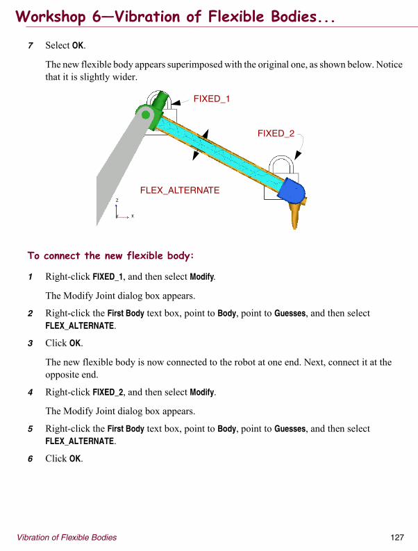
Vibration of Flexible Bodies 127
7 Select OK.
The new flexible body appears superimposed with the original one, as shown below. Notice that it is slightly wider.
To connect the new flexible body:
1 Right-click FIXED_1, and then select Modify.
The Modify Joint dialog box appears.
2 Right-click the First Body text box, point to Body, point to Guesses, and then select FLEX_ALTERNATE.
3 Click OK.
The new flexible body is now connected to the robot at one end. Next, connect it at the opposite end.
4 Right-click FIXED_2, and then select Modify.
The Modify Joint dialog box appears.
5 Right-click the First Body text box, point to Body, point to Guesses, and then select FLEX_ALTERNATE.
6 Click OK.
FLEX_ALTERNATE
FIXED_1
FIXED_2
Workshop 6�Vibration of Flexible Bodies...

128 Vibration of Flexible Bodies
To delete the old flexible body:
� Right-click the flexible body, point to FLEX_BODY_5, and then select Delete.
To set visualization attributes for the new flexible body:
� Set the datum node and color deformations for the new flexible body by importing the file datum_and_color.cmd from the misc subdirectory.
To perform frequency response on the alternate forearm design:
1 Display the Perform Vibration Analysis dialog box.
2 From the Vibration Analysis list, select New Vibration Analysis.
3 In the corresponding text box, enter .table.Alternate_Design.
4 Set Simulation Script to TIME_DOMAIN_SCRIPT_2.
5 Select Import Settings from Existing Vibration Analysis, and select One_Second.
6 Click OK.�
7 Launch ADAMS/PostProcessor.
8 Create a new page.
9 Right-click the viewport and select Load Plot.
10 Set Source to Frequency Response.
11 From the Vibration Analysis list, select One_Second and Alternate_Design.
12 From the Input Channels list, select Input_Channel_1.
13 From the Output Channels list, select Output_Channel_Y.
14 Select Magnitude.
15 Select Add Curves.
� Some DOS windows will appear on the screen as the .mtx files are being generated for the new flexiblebody.
Workshop 6�Vibration of Flexible Bodies...

Vibration of Flexible Bodies 129
16 Were you able to reduce the magnitude of the resonance peak at 121.7 Hz with the alternate design?
______ Yes ______ No
17 Create a new page, load the vibration animation for Alternate_Design and animate the forced vibration at 121.7 Hz in a zoomed isometric view.
18 Is the mode at 121.7 Hz still vibrating with coupled vertical and translational motion?
_______ Yes ______ No
Wrap up
To wrap up:
1 Close ADAMS/PostProcessor.
2 Save your model in binary format.
3 Exit ADAMS/View.
Optional tasks� Perform a normal-mode animation and review the mode shapes.
Workshop 6�Vibration of Flexible Bodies...

130 Vibration of Flexible Bodies
Workshop 6�Vibration of Flexible Bodies...

131
7 USING DESIGN EVALUATION TO MINIMIZE FREQUENCY RESPONSE
Minimize the vertical acceleration of a rail bogie across the frequency range of 0.1 to 80 hertz.
What�s in this module:� What ADAMS/View Requires, 132
� Types of ADAMS/Vibration Macros, 133
� Design Objective Details, 134
� Dialog Box Cascade, 135
� Other Considerations, 136
� Workshop 7—Design Evaluation, 137

132 Using Design Evaluation to Minimize Frequency Response
� Model that has been parameterized with design variables *
� Multi-run script that runs a vibration analysis
� Design objective
Tip: Use the /View variable and Vibration Macro option
*ADAMS/Insight will also accept design points.
What ADAMS/View Requires

Using Design Evaluation to Minimize Frequency Response 133
� There are four built-in ADAMS/Vibration macros:
� Frequency Response: 1 Input, 1 Output
� Frequency Response: All Inputs, 1 Output
� PSD: 1 Output
� Modal Participation: 1 Input, 1 Output
Types of ADAMS/Vibration Macros

134 Using Design Evaluation to Minimize Frequency Response
� The design objective is defined by a macro and design variable.
� The macro is run at the end of the simulation and performs whatever computations and commands it contains.
� Matrix operations, summations, result set data indexing, temporary storage of data, and so on.
� Eventually, the results must be reduced to a single value, representing the objective.
� This value is then stored in the design variable.
� The design variable returns the value to the objective.
Design Objective Details

Using Design Evaluation to Minimize Frequency Response 135
Here�s the cascade of dialog boxes that you�ll see:�
� Review the dialog boxes and ask the students if they have any questions.
Dialog Box Cascade

136 Using Design Evaluation to Minimize Frequency Response
� Often, vibration issues must be balanced with other design considerations. Therefore, you may want to have more than one design objective included in your design evaluations.
� Design study
� Allows multiple design objectives
� DOE
� Allows multiple design objectives
� Optimization
� Can only have a single design objective.
� You can, however, define a weighted �cost� function to effectively study multiple objectives, c1, c2, c3
� For example: Cost = 3*(c1)**2 + 2*ABS(c2) + 10*ABS(c3)
� Modify the macro to suit your needs.
Other Considerations

Using Design Evaluation to Minimize Frequency Response 137
This workshop takes about 45 minutes to complete.
Problem statementMinimize the vertical acceleration of a rail bogie across the frequency range of 0.1 to 80 hertz.
In this workshop, you will learn how to use design evaluation tools to improve your designs. You will take a model that has been instrumented for vibration analysis and create an objective function and a multi-run simulation script. You will also perform a design study of suspension parameters. Then, you will use optimization to find the combination of parameter variables that will minimize the vertical acceleration of the bogie.
XII III
III
IVVVIVII
XXI
VIII
IX
Workshop 7�Design Evaluation

138 Using Design Evaluation to Minimize Frequency Response
Model description� The model represents a rail bogie with two wheelsets and suspension.
� The model has seven moving parts (not including ground).
� Four revolute joints constrain the wheelsets to the arms.
� The suspension springs connecting arms to the frame are represented with fields; other attachment points use bushings. Dampers between the frame and arms are modeled with SFORCEs.
� Wheel-to-rail interaction is simplified with linear bushing forces.
� Vibration input channels at the four wheels apply vibration forces vertically through a swept sine actuator.
� The output channel is defined to be the vertical acceleration of the frame center-of-mass.
Some parameters of the bogie design have been parameterized as detailed below:
Category: Design Variable: Description:
Stiffness coefficients for FIELDs
K11, K22, K33, K44, K55
Diagonal entries for stiffness matrices of FIELDs: SPRING_MAIN_FL, SPRING_MAIN_FR, SPRING_MAIN_RL, SPRING_MAIN_RR, representing three translational and two torsional stiffness coefficients.
Damping ratio for FIELDs
FLD_C_RATIO Damping ratio for all fields.
Stiffness and damping for BUSHINGs between wheel and rail (ground)
RAIL_STIFFRAIL_DAMP
Translational stiffness coefficient for bushings: FL_BUSH, FR_BUSH, RL_BUSH, RR_BUSH. Translational damping coefficient for bushings: FL_BUSH, FR_BUSH, RL_BUSH, RR_BUSH.
Workshop 7�Design Evaluation...

Using Design Evaluation to Minimize Frequency Response 139
Getting startedFirst, you start ADAMS/View and import the model. Then you inspect an input channel, an output channel, and a vibration analysis.
To import the model:
1 Start ADAMS/View from the working directory exercise_dir/mod_07_bogie.
2 Import the model bogie_start.cmd.
The bogie model appears in a rendered isometric view.
To inspect an input channel:
1 Locate an input channel at one of the wheels, right-click and select it.
2 From the Edit menu, select Modify.
The Modify Input Channel dialog box appears with your input channel and its definitions.
3 Inspect the settings for the input channel, noting that a swept sine is being applied to a marker on the wheelset. A force magnitude of 1000.0 N is being applied in the local z direction with zero phase angle.
4 Select Cancel.
5 Clear the select list.
To inspect an output channel:
1 From the Build menu, point to ADAMS/Vibration, point to Output Channel, and then select Modify.
2 From the Database Navigator, select Output_Channel_1.
3 Inspect the settings for the output channel, noting that acceleration of the wheelset is being measured in the global z direction.
4 Select Cancel.
Workshop 7�Design Evaluation...

140 Using Design Evaluation to Minimize Frequency Response
To inspect the vibration analysis specification:
1 From the Simulate menu, point to ADAMS/Vibration, and then select Vibration Analysis.
2 From the New Vibration Analysis list, select Vibration Analysis.
3 Right-click the text box, point to Vibration Analysis, point to Guesses, and then select Baseline.
4 Inspect the analysis specifications, and complete the following:
� The __________ vibration analysis will linearize the model about the ____________ operating point.
� Damping will be ___________ and ______ steps will be used across a frequency range of ________ to ________ hertz.
5 Close the dialog box without running the analysis.
Setting up for the design studyTo perform a design study or another multi-run simulation with ADAMS/Vibration, you must define your simulation script properly. To do this, you'll use a customized dialog box.�After creating the script, you inspect it to learn what commands it uses. Then, you test this script, using it to analyze the model in its baseline configuration. Finally, briefly review the frequency response plot for the baseline analysis. This time we won't give you the detailed steps for creating the plot.
To create the multi-run simulation script:
1 Load the script-creating dialog box by importing the file cre_vib_solve_script_dlg.cmd from the dbox subdirectory.
The Create Vibration Multi-Run Script appears.
2 In the Sim Script Name text box, enter VIBRATION_SOLVE_MULTIRUN.
3 Right-click the Vibration Analysis Name text box, point to Vibration Analysis, point to Guesses, and then select Baseline.
The dialog box updates with the frequency range parameters.
4 Select Logarithmic Spacing of Steps.
5 Select OK.
The multi-run script is created.
� Mention that the file for the custom dialog box is also included in the ADAMS/Vibration installation directory: \install_dir\vibration\examples\macros.
Workshop 7�Design Evaluation...

Using Design Evaluation to Minimize Frequency Response 141
To inspect the multi-run simulation script:
1 From the Simulate menu, point to Simulation Script, and then select Modify.
2 In the Database Navigator, choose the script named VIBRATION_SOLVE_MULTIRUN.
The Modify Simulation Script dialog box appears with the commands as shown below:
3 Briefly review the commands and see if they make sense to you.
4 Select Cancel.
To test the script:
1 From the Simulate menu, point to Scripted Controls.
The Scripted Controls dialog box appears with your VIBRATION_SOLVE_MULTIRUN script in the text box.
2 To perform the baseline analysis, select the Start Simulation tool.
If no error messages appear, your simulation was successful.
3 Close the Simulation Control dialog box.
Workshop 7�Design Evaluation...
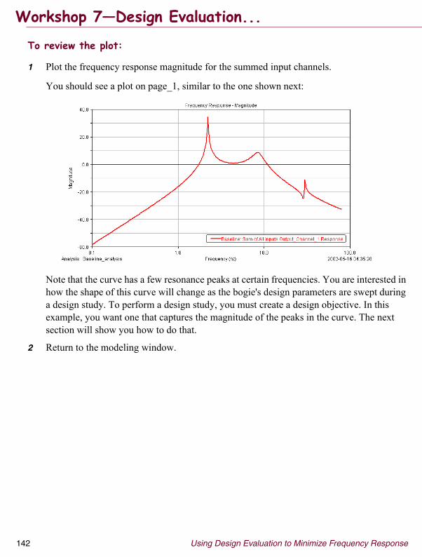
142 Using Design Evaluation to Minimize Frequency Response
To review the plot:
1 Plot the frequency response magnitude for the summed input channels.
You should see a plot on page_1, similar to the one shown next:
Note that the curve has a few resonance peaks at certain frequencies. You are interested in how the shape of this curve will change as the bogie's design parameters are swept during a design study. To perform a design study, you must create a design objective. In this example, you want one that captures the magnitude of the peaks in the curve. The next section will show you how to do that.
2 Return to the modeling window.
Workshop 7�Design Evaluation...

Using Design Evaluation to Minimize Frequency Response 143
Creating a design objective, macro, and ADAMS/View design variableCreating the design objective for a vibration analysis is a multi-step process. You need to create three new items: an ADAMS/View design variable, a macro, and finally the objective, which requires the first two items. The macro does the majority of the work as it calculates the value of interest; the variable is used to store the calculated value and to pass it on (or return it) to the objective.
To create a design objective, macro, and ADAMS/View design variable:
1 From the Simulate menu, point to Design Objective, and then select New.
The Create Design Objective dialog box appears.
2 In the Name text box, enter MAX_FRAME_CM_ACC.
3 From the Definition by list, select /View Variable and Vibration Macro.
The Create Vibration Design Objective Macro dialog box appears.
4 In the Macro Name text box, enter eval_fva_results.
5 Right-click the Return Value Variable text box, point to Variable, and then select Create.
The Create Design Variable dialog box appears.
6 In the Name text box, enter FVA_RESPONSE_VARIABLE.
7 From the Type list, select Real.
8 From the Units list, select Acceleration.
9 Leave all other settings at their defaults.
10 Select OK.
The dialog box closes and the name of variable, FVA_RESPONSE_VARIABLE, is placed in the Create Vibration Design Objective Macro dialog box.
11 From the Target Vibration Data list, select Frequency Response: All Inputs, 1 Output.
12 Right-click the Output Channel text box, point to Output Channel, point to Guesses, and then select Output_Channel_1.
13 Select Maximum.
14 Select All Frequencies.
Workshop 7�Design Evaluation...

144 Using Design Evaluation to Minimize Frequency Response
15 Select OK.
The dialog box closes and both the macro name, eval_fva_results, and the name of variable, FVA_RESPONSE_VARIABLE, are placed in the Create Design Objective dialog box.
16 Select OK.
The design objective and all its dependencies have been created. To review, a cascade of what you've created is like this:
Workshop 7�Design Evaluation...

Using Design Evaluation to Minimize Frequency Response 145
Evaluating a design objectiveAfter you create an objective, it is always a good idea to test it to make sure it is calculating everything as you expect before using it in a design evaluation. Here, you'll use a custom menu button to simplify the process of evaluating the design objective.
To evaluate a design objective:
1 Load the custom menu button by doing the following:
� Use the F2 key to import the file eval_menu_buttons_full_errchk.cmd from the utils/obj_eval_menu subdirectory.
2 From the Simulate menu, point to Design Objective, and then select Evaluate.
The Command Window and the Optimize Objective Evaluate dialog box appear.
3 Double-click the Objective Name text box and select MAX_FRAME_CM_ACC.
4 Double-click the Analysis Name text box and select Baseline_analysis.
5 Select OK.
The value of the evaluated objective is written to the command window:�
.bogie.MAX_FRAME_CM_ACC(.bogie.Baseline_analysis) = 54.5498542569 (meter/sec**2)
Preparing output settings for saving individual runsTo plot the results of the individual analyses, you must ask for them to be stored in the database.
To prepare the output settings:
1 From the Settings menu, point to Solver, and then select Output.
The Solver Settings dialog box appears.
2 Select More.
3 Set Output Category to Database Storage.
4 Under Individual Simulations, set Save Analysis to Yes.
5 Under Multi-Run Simulations, set Save Analysis to Yes.
6 Select Close.
This will permit different frequency responses to be plotted one over the other at the end of the design study analysis.
� If students want to compare the evaluated value to what is shown in a frequency response plot, they willhave to change the plot's vertical axis to a linear scale.
Workshop 7�Design Evaluation...

146 Using Design Evaluation to Minimize Frequency Response
Performing a design study analysisNext, you study and plot the effect of the design variable K11, a suspension stiffness parameter representing the first diagonal entry in the stiffness matrix for the fields. You will plot the frequency response for the five trials, one on top of the other. By doing this you'll be able to see the effect of the design change.
To study the effect of K11:
1 From the Simulate menu, select Design Evaluation.
2 Direct the design study to objective MAX_FRAME_CM_ACC by completing the Design Evaluation Tools dialog box as follows:
3 Select Start.
The design study runs and plots the objective versus design variable for each trial in the design study as shown below:
� Model: .bogie
� Simulation Script: VIBRATION_SOLVE_MULTIRUN
� Study a Objective: MAX_FRAME_CM_ACC
� Select Design Study
� Design Variable: K11
� Default Levels: 5Make sure you use this script.
Workshop 7�Design Evaluation...

Using Design Evaluation to Minimize Frequency Response 147
To plot the effect of K11:
1 Launch ADAMS/Postprocessor.
Tip: Make sure ADAMS/View is the active window.2 Create a new page.
3 Set Source to Frequency Response.
4 From the Simulation list, drag-select the five runs Baseline_1 through Baseline_5.
Note: Don't select Baseline.
5 Select Sum all Input Channels.
6 From the Output Channels list, select Ouput_Channel_1.
7 Select Magnitude.
8 Select Add Curves.
The plot should look like the following. You may have to move the legend.
9 Describe what appears to be the main effect of the design variable, K11.
______________________________________________________________________
______________________________________________________________________
10 Return to the modeling window.
Workshop 7�Design Evaluation...

148 Using Design Evaluation to Minimize Frequency Response
Studying the effect of K33In this section, you study the effect of the design variable K33, a suspension stiffness parameter representing the third diagonal entry in the stiffness matrix for the fields. Then, review the frequency response results.
To study the effect of K33:
1 To study the effect of K33, prepare the design study as follows:
� Model: .bogie
� Simulation Script: VIBRATION_SOLVE_MULTIRUN
� Study a Objective: MAX_FRAME_CM_ACC
� Select Design Study
� Design Variable: K33
� Default Levels: 5
2 Select Start.
The plot displays as shown below:
To review the results of K33 design study:
1 Launch ADAMS/Postprocessor.
Tip: Make sure ADAMS/View is the active window.2 Create a new page.
3 Set Source to Frequency Response.
Workshop 7�Design Evaluation...

Using Design Evaluation to Minimize Frequency Response 149
4 From the Simulation list, drag-select the last five runs, Baseline_6 through Baseline_10.
5 Select Sum all Input Channels.
6 From the Output Channels list, select Ouput_Channel_1.
7 Select Magnitude.
8 Select Add Curves.
The plot should look like the following. You may have to move the legend.
9 What appear to be the main effects that parameter K33 has on the vertical acceleration of the bogie?
________________________________________________________________________
________________________________________________________________________
10 Return to the modeling window.
Workshop 7�Design Evaluation...

150 Using Design Evaluation to Minimize Frequency Response
Performing an optimization analysisTo try and minimize the vertical acceleration, you can perform a design optimization with both parameter variables. Then, perform a confirmation run to see whether or not the results show an improvement.
To optimize the design for minimized vertical acceleration:
1 Prepare the optimization study as follows:
2 Select Optimizer.
The Solver Settings dialog box displays the Optimization options.
3 Select More.
4 In the Tolerance text box, enter 1.0E-5.
5 In the Increment text box, enter 1.0E-4.
6 Close the Solver Settings dialog box.
7 Select Start.
The command window displays output from the optimizer, showing how it's progressing.
� Model: .bogie
� Simulation Script: VIBRATION_SOLVE_MULTIRUN
� Study a Objective: MAX_FRAME_CM_ACC
� Select Optimization
� Design Variables: K11,K33
� Goal: Minimize Des. Meas. / Objective
Starting optimization iteration: 2Computing gradients/performing line search. Iteration: 2 Pass: 1 Objective 1 = 5.975601e+000Computing gradients/performing line search. Iteration: 2 Pass: 2 Objective 1 = 5.953365e+000OptDes GRG: feasible, K-T satisfiedThe optimization has terminated.Total optimization analysis calls: 9
Workshop 7�Design Evaluation...
Using Design Evaluation to Minimize Frequency Response 151
8 Close the dialog box that tells you the optimization is successful.
When the optimizer has finished, the design variables K11 and K33 are set to the values that the optimizer had determined to be optimal for the given optimizer settings.
To perform a confirmation vibration analysis:
1 From the Main Toolbox, double-click the Select tool to reset the model.
2 From the Simulate menu, point to ADAMS/Vibration, and then select Vibration Analysis.
3 In the New Vibration Analysis text box, enter Optimized.
4 Select Import Settings from Existing Vibration Analysis.
5 From the Database Navigator, double-click Baseline.
ADAMS/Vibration updates the vibration analysis specifications.
6 Select OK.
Reviewing results of the optimization studyIn this section, you compare the frequency response results of the baseline analysis with the optimized analysis.
To review the results:
1 Launch ADAMS/PostProcessor.
2 From the treeview, select Page_1.
3 Set Source to Frequency Response.
4 From the Vibration Analysis list, scroll up and select Optimized.
5 Select Sum all Input Channels.
6 From the Output Channels list, select Ouput_Channel_1.
7 Select Magnitude.
Workshop 7�Design Evaluation...

152 Using Design Evaluation to Minimize Frequency Response
8 Select Add Curves.
The plot should look like the following. You may have to move the legend.
Here you can see that the optimizer has indeed found a combination of K11 and K33 that minimizes the maximum acceleration peak across the frequency spectrum.
Wrap up
To wrap up:
1 Close ADAMS/PostProcessor.
2 Delete the simulation results you are not interested in.
3 Save your database.
4 Exit ADAMS/View.
Optional tasks1 Perform a forced vibration animation and review the behavior at frequency peaks.
Hint: Use a Maximum Translation value of 0.05.
2 Perform a normal mode animation and review the mode shapes.�
� Summarize what they learned in this course:-Different input/output channel types-Different vibration actuator types-How ADAMS models can be set up for vibration analyses-Performing design evaluation using frequency-domain objectives-Performing frequency-domain analyses:
-The different types of results that can be obtained-How frequency-domain analyses can be integrated with design tools in ADAMS
-How to set up models for frequency-response computation
Workshop 7�Design Evaluation...

153
A THEORY
This appendix shows equations that ADAMS/Vibration uses in performing its calculations.
What�s in this appendix:� Introduction, 154
� Vibration Actuators, 155
� Analysis Methods, 157

154 Theory
IntroductionTo reduce a nonlinear model to a linear form, ADAMS/Vibration performs an eigensolution on the nonlinear model. The iterative eigensolver in ADAMS/Vibration uses the complete set of model modes to converge to a subset of modes within the specified error tolerance. The canonical form1�of the linear model is constructed from this subset of model modes. For some small models, ADAMS/Vibration may not compute the desired number of modes. If you want to view the complete set of model modes, use ADAMS/Linear.
ADAMS/Vibration creates linearized models from nonlinear ADAMS models in the form of: = Ax + Bu
y = Cx + Du
where:
� is the modal state of the linearized model
� u is the input applied to the model
� y is the output from the model
A, B, C, and D are collectively called state matrices for the model.
Input channels define inputs to the linearized model, and output channels define outputs from the model. The linearization process automatically determines the states of the linearized models which correspond to the modes of the model.
•. 1De Silva, Clarence W., “Vibration Fundamentals and Practice”, CRC Press 2000.
x·
x·

Theory 155
Vibration ActuatorsThis section describes the calculations for the various vibration actuators ADAMS/Vibration uses. Included are:
� Swept Sine
� Rotating Mass
� User-Defined Function
� Power Spectral Density
Swept SineSwept sine defines a constant amplitude sine function being applied to the model. The amplitude of the sine function and the starting phase angle are required and must be specified on the Create Vibration Actuator dialog box.
where:
� f is the forcing function
� F is the magnitude of the force
� is the phase angle
Rotating MassA rotating mass applies a frequency-dependent force. This actuator represents the force due to a rotating mass located at a specified offset from an axis of rotation. The axis of rotation is defined by the input channel that this vibrational actuator is applied to.
where:
� is the frequency
� f is the unbalanced mass forcing function
� m is the unbalanced mass
� r is the radial distance of the unbalanced mass from the axis of rotation
f ω( ) F= θ( ) j+ θ( )sin⋅cos[ ]⋅
ω( )
θ
f ω( ) m ω2 r⋅ ⋅=
ω
ω( )

156 Theory
Vibration Actuators...Similarly, a rotating mass placed at a distance offset along the axis of rotation results in an unbalanced moment.
where:
� t is the moment due to unbalanced mass with offset
� d is the distance of the unbalanced mass perpendicular to the plane
User-Defined FunctionYou can define any function of the independent variable omega:
where:
� is the frequency
� g is the general function of omega
Power Spectral DensityThe vibration actuator PSD is defined using a spline function. The PSD dialog box allows for the spline function to specify either a force PSD or a displacement PSD. For the displacement PSD, a corresponding stiffness must also be specified.
It is assumed that the PSD inputs applied to the linear model are not correlated to one another.
Note: You cannot combine vibration actuators of the non-PSD-type with PSD-type vibration actuators in the same vibration analysis.
t ω( ) m ω2 r d⋅ ⋅ ⋅=
ω( )
f ω( ) g ω( )=
ω
ω( )

Theory 157
Analysis MethodsThis section describes the calculations for the analysis methods used in ADAMS/Vibration. Included are:
� Frequency Response
� Modal Coordinates Computation
� PSD Computation
Frequency ResponseFor frequency response computation, the linearized model is represented as:
x(s) = Ax(s) + Bu(s)
y(s) = Cx(s) + Du(s)
where s is the Laplace variable
The system transfer function can be represented as:
where:
� H(s) is the transfer function for the model
� I is the identity matrix of dimension equal to the number of system states
For a given vibration analysis, the system frequency response is given as:
Modal Coordinates ComputationModes most active in a frequency response can be identified from the modal coordinates. The modal coordinates are computed as:
H s( ) y s( )u s( )---------- C sI A–( ) 1– B D+= =
y s( ) H s( )u s( )=
x s( ) sI A–( ) 1– B=

158 Theory
Analysis Methods...
PSD ComputationPSD of output channels for given input PSDs is given as:
where:
� p(s) is the matrix of power spectral density
� H*(s) is the complex conjugate transpose of H(s)
� U(s) is the matrix of input spectral density
The matrix of input spectral densities is a diagonal matrix with the vibration actuator PSDs on the diagonal locations.
p s( ) H∗ s( ) U s( ) H s( )⋅ ⋅=

159
B ANSWER KEY
This appendix contains the answers to the questions listed in this training guide.
What�s in this appendix:� Answers for workshop 1, 160
� Answers for workshop 2, 160
� Answers for workshop 3, 160
� Answers for workshop 4, 160
� Answers for workshop 5, 161
� Answers for workshop 6, 162
� Answers for workshop 7, 162

160 Answer Key
Answer Key
Answers for workshop 1Step 8 on page 33: 4.3186 and 5.6078
Answers for workshop 2Step 15, page 55: 5
Step 16, page 55: 100
Step 17, page 55: Yes.
Answers for workshop 3Step 9, page 69: No, 50 output steps is not quite enough for the frequency range.
Step 10, page 69: You are seeing a rounding-off effect in the plotter due to the vertical axis Db scale. If you set the vaxis scale to "linear" you'll see the full lower bound of the results data.
Step 11, page 69: It wouldn't be able to solve beyond 10 Hz.
Step 3, page 71:
� Peaks: 1.5483, 4.4052, 5.4964, 9.2263 Hz
� Valleys: 1.9451, 4.5838, 9.0874 Hz
Step 10, page 74: Out of phase. The damping characteristics at each wheel are different enough that the wheels cannot respond in the same manner, even though the input variation is the same.
Answers for workshop 4Step 8, page 89: 8

Answer Key 161
Answer Key...
Answers for workshop 5Step 7 on page 101:
� Hop: mode #2= 22.2608 Hz
� Heave: mode #1=0.9436 Hz
� Nibble: mode #3=81.0983 Hz
Step 13, page 105: 0.9403, 22.2754, 81.2267
Step 14, page 106: No
Step 15, page 106: In this model, to emphasize the peaks, the damping coefficients for the bushings and spring are either very small or have been set to zero. Therefore, in this case you're not simply seeing differences due to damping effects. Instead, this is an aliasing or resolution issue. For this vibration analysis, the resolution of output data was set to 300 logarithmically spaced steps. This is not enough to capture the exact frequency of the peaks in the curve. Although you are near the absolute peak, you're not quite there. By solving with more output steps (for example, 5000) you will get closer to the frequencies calculated in the normal-modes analysis.
Step 5, page 110: EIGEN_3
Step 8, page 111: Mode 3 (126.756 newton-mm)
Step 9, page 111: Spindle, Z (vertical)
Step 10, page 111: Spindle, Y (lateral)
Step 11, page 113: True. Wheel hop vibration has been reduced.
Step 12, page 113: False. The driver will feel less vibration.
Step 13, page 113: True. Chassis heave magnitude has increased.
Step 14, page 113: True. The frequency of heave has shifted lower.

162 Answer Key
Answer Key...
Answers for workshop 6Step 3, page 123: 3 seconds
Step 5, page 124: 10.562 Hz, 21.0 Hz
Step 7, page 124: 117.2 Hz to 121.7 Hz
Step 8, page 125: The 1.0-second operating point
Step 16, page 129: Yes
Step 18, page 129: No
Answers for workshop 7Step 4 on page 140:
� The forced vibration analysis will linearize the model about the static operating point.
� Damping will be included and 400 steps will be used across a frequency range of 0.1 to 80 hertz.
Step 9, page 147: The main effect of K11 is to shift the frequency of the second peak and to reduce the magnitude of the higher frequencies. The lower frequency peak isn�t affected as dramatically.
Step 9, page 149: The main effects of parameter K33:
� To alter the acceleration magnitude at all three frequency peaks.
� The frequency of the second peak has been shifted significantly, and the third peak has either been diminished or pushed out of this frequency spectrum entirely.


![Attachment 1 contains proprietary information. · 2012. 7. 19. · ADAMS Database ML051440097). [5] 26A6492R2-NP, Steam Dryer Vibration Instrument Installation Procedure, April 2005](https://img.pdfslide.us/doc/110x75/6114305b81070f3d22208e72/attachment-1-contains-proprietary-2012-7-19-adams-database-ml051440097.jpg)