Embed Size (px)
Citation preview
AD-A016 772
COMPUTER SIMULATION OF RANDOM ATMOSPHERICALLY DEGRADED OPTICAL BEAMS
S. A. Collins, Jr., et al
Ohio State University
Prepared for:
Rome Air Development Center Defense Advanced Research Projects Agency
September 1975
DISTRIBUTED BY:
urn National Technical Information Service U. S. DEPARTMENT OF COMMERCE
wmm
315122
N N CO
RAOC-TR-75-222 Unal Technical Report September 1975
COMPUTER SIMULATION OF RANDOM ATMOSPHERICALLY DEGRADED OPTICAL BEAMS
Ohio State University
Sponsored by Defense Advanced Research Projects Agency
AKPA Order Mo. 2646
Approved for public release; distribution unlimited.
The views and conclusions contained In this document sre those of the suthors and should not be Interpreted as necessarily representing the. official policies, either expressed or Implied, of the Defense Advsnced Research Projects Agency or the U. S. Government.
NATIONAL TECHNICAL INFORMATION SERVICE
us :;»[.•"••-■ I «•>«« ■,l ■ s'.'^d, V* /.'IM
Rome Air Development Center Air Force Systems Comand
Grifflas Air Force Base, Mew York 13441
\
.- , r1' ü1*0" h*8 b*en revlewed by the RADC Information Office (01) »nA i* *\tThl\t0 the NatlOMl Techni"l Information Service (NTIS) At OTI«- it will be releaaable to the general public including foreign nItLns
Thi. report ha. been reviewed and 1. approved for publication.
!
ß APPROVED:
DARRYB P. GREENVWOD, Capt, USAF Project Engineer
ictx t. -'
r» ■ • a t: i n i»' a
n »
j Do not return this copy. Retain or destroy.
'■ ' '
^
COMPUTER SIMULATION OF RANDOM ATMOSPHERICALLY DEGRADED OPTICAL BEAMS
S. A. Collins, Jr. ü. D< Duncan
Contractor: uhio 8t«t« L'n'. versity Contract Numbt-r: F.JÜ6ÜJ-7"-C-0130 Efffctive Date ot Contract: 24 January 1974 Contract Expiration Uatt-: 14 January 197S Amount ot Contract: $30,000.00 I'rü^ram Co4« Number: 4E20 Period ol work covered: J4 Jan 74 - 14 Jan 75 '
rrimipal Investigator: Dr. Stuart A. d 111ns, Jr, Phone: M4 422-5045
Project EnginMn Capt Darryl P. Creenwood ' Phone: 315 330-3145
Approved for public release; distribution unlimited.
Ihis research^uas supported by the Defense Advanced Research Projects Agency of the Department of Detense and was monitored by Capt Darryl P. Creenwood, RADC (0C8B), Criffiss Air Pore« Base, New York 13441.
I.
.

■«p
mcuasiLua
REPORT DOCUMENTATION PAGE I MPOVT S UR»H
RAl)i:-lK-7i-JJJ
.' OOVT »C t tSSION HO
COMTOTEI SIMILATIOi 01 RANDOM AlMuSI'HKRlCAI.LY DEGIADED OPTICAL HKAMS
' iüTMÖfiTä S. A. Collins, Jr. ü. D. Dua« in
RKAI) INSTHl'( TIONS BEFOIIE COMPLETINa H>RM
1 HECl^ltNT't CATALOG HUMalM
» TyPf of »IPOBT 4 PtHIOD COVIRfD
Kliiiil Ti'ctinlial Report 24 .Ian 74 - 14 Jan 75
t pmroBMiNO OBO RCPOPT «UMBEH
(JÖ6J-2) t nt,T»«CT OP CiR»NT NuMBfR
Fiü6Ü2-74-C-0130
Ohio State I'niverslty Elcctto SciWM« Laboratory 1 320 Kinm-ar Rd, Columbus Oi 4 12 12
'P PBO'-.»»M I L €«irNT PBOJl"'^ '»S« »Bf * ■> «0»« UNIT •. MI.( I.
62J01E 26460101
S'BC.I.INO CflTf S»M> MlO »DC'BtSS
DcfcBM Advanci'il Kesearth i'rojt-its A^eiu y UÜU Wilson lilvd Arlington VA 22209
', BrPDB' BATI
September 1975
•4 M~s T~B s j AOCNO SAMt « »^TBrS' it littrfW Irm I' nlr Hint <>tli
lOW Air Development (enter (OCSE) Griffloa ATI NY I 1441
') BJMBEB C' P AOC.S ^ ^P < 67 '? ^rCjBiTY f. L*4S ..( ffn r,r, „
L-NCLASS1FIKD
N/A
'!• .'ECLASSiriC/lTiO"» DO«NOI»*DINO i.'.xEDuLf
Approved li^r public releasi-; distribution unli-nlted.
I 0lS''BtBJ'lOS5T»TFMfNT 'l^. «f.'f. t m'r„.l ,n HI ■■ * .■■ . H >r(frf»n( /»on- f(ff...ft.
S.irae
I S„PP, fMts-»Rr SO'f S
RADC Project Kn>;ineer. C«pt Darryl F. Crooawood/OCSE
I'ropa^at Ion optical Atmospheric Si^.ulat ion Coaputor
i' A BS T M AC i.J ■ 1*i.'»f\ t* tl * fiifr/pf
In th opt i i ross laagt An ex ■colo f lu< t
is report tliere !s developed a sihi'tne for simulating randomly degraded al beams im hiding bot t piiase and i.)^,-amp 1 i t mle and the effect of their
•orrelation The scheme works for optical degradations whose scale hs ran^'f from much smaller to much larger than the input aperture size. tension of the well-knowr Fourier transform method is used for the small fluctuations and a polynomial approach Is used for the larger scale
uations. •
ÜL DD '.r., 1473 t :,<'■',H nf I NI< «.\ is '■JH'. ,^' 't
UNCLASSIFIED SICU«lTv CLASSirirtTiON rit TMIS PAGE tWhm Itmlmfnlrtnl
WWW,IIIJl ****
CONTENTS
1. INTRODUCTION
2. GENERAL STATEMENT OF PROBLEM AND FREQUENCY DIVISION
3. HIGH SPATIAL FREQUENCY REPRESENTATION
4. LOW SPATIAL FREQUENCY REPRESENTATIONS
5. RESULTS
6. SUMMARY
7. CONCLUSIONS
APPENDIX A - SPECTRA
APPENDIX B
APPENDIX C
APPENDIX D
REFERENCES
Page
1
2
8
12
19
43
45
47
56
60
62
63

t^m^m
This report deals with the digital simulation of optical wavcfronts which have been degraded by propagation through a turbulent atmosphere ' Such simu ated wavefronts are necessary in the computer simulation ot optical systems operating on atmospherically degraded light Such system simulation is very desirable because of the expense of building prototype systems and testing them at remote locations after construction The prime motivation is computer testing of compensated imaging systems for viewing objects at extremely large distances through the atmosphere.
The computer generated wavefronts to be described here are characterized by other factors. They simulate light which has propagated vertically through the atmosphere and have as a result an extremely long outer
and ?hP IfwTnfrHtS alS0 inclu?e a'!'Pmude as well as phase fluctuations and the effect of the cross correlation between them.
1. INTRODUCTIOf;
In the past, two technigues have been used to generate members of random ensembles: the Fourier transform techniguc and the orthogonal polynomial techmgue. In the Fourier transform technigue the power spectrum of the random function is assumed known. An array of uncorrelated gaussian random numbers with zero mean and unit variance is generated using standard digital computer programs. The Fourier transform of the array is computed and multiplied by the square root of the power spectrum and the inverse Fourier transform of the product is computed • he resu.ting array still has gaussian random variables but the correl'ation function is now that related to the power spectrum as desired.
In the orthogonal polynomial technique the random function is represented as a sun of orthogonal polynomials, with random coefficients For example one might use Zernike polynomials to represent a random function in a round aperture. This scheme is frought with peril however. unless the polynomials happen be statistically independent. Otherwise there wil1 be cross-correlation between the various polynomial coefficients. loro^- Surau apprf,ath would USP t-he Karhunen-Loeve technigue (Davenport, 1958) in whTch a set of polynomials is qenerated which are eigenfunctions of the covanance function. The random function is then expanded as * series of these eigenfunctions. Coefficients of the eigenfunctions are then known to be statistically independent.
Simultation of random atmospheric quantities has been performed using the Fourier transform technique (Hogge, 1973), (Bradley, 1974) where refractive index variations were generated. The Fourier transform technique h?s also ueen used (McGlammery, 1974), (Brown, 1974) for the simulation of respectively two and one dimensional random phase fronts.
Random wavefronts have also been generated using a sum of 7ernike polynomials (Noll, 1974) and the Cholesky decomposition (Bradley. 1974) The work herein also related to the wavefront polynomial fitting scheme of Fried (1965) and to general work on Karhunen-Loeve series.

In this report we extend previous work in that both log-amplitude as well as phase are considered as well as their cross-correlation. We also consider spatial spectra of much larger frequency range than heretofore used. The result is an approach which combines both the polynomial and Fourier transform technique approaches in an optimum fashion.
In this paper a random wavefront is represented as the sum of several terms, each pertaining to a different spatial frequency range. In each range a technique appropriate to the range is used to generate ooth phase and log-amplitude fronts. In the highest spatial frequency range the Fourier transform technique is used, extended to produce phase as well as log-amplitude fronts. In the lower spatial frequency '•anges wnere the fluctuations are less rapid a polynomial scheme is used which starts out with a set of polynomials similar to Fried's but including more terms and ends up with the statistically independent Karhunen-Loeve polynomial-;. These are then summed with random independent coefficients to provide a particular manifestation.
In the balance of the paper we will first present the physical picture considered along with a description of the spectral separation technique. Then the high frequency problem will be considered, in- cluding coupled phase and log-amplitude. In the next section the development of the polynomial fitting scheme used for the lower spatial frequency ranges will be presented. This will include the generation of a set of polynomials and their diagonalization to form the Karhunen- Loeve functions. Following that the result of all the techniques is demonstrated and a typical representation shown. The final section contains discussion, summary and conclusions.
2. GENERAL STATEMENT OF PROBLEM AND FREQUENCY DIVISION
The general physical picture which we are considering is shown in Fig. 1 where we see a light beam propagating from a great height down through an atmosphere with fluctuating refractive index to the input aperture of an optical system. It is assumed that the outer scale LQ and the structure parameter Cf5 of the turbulent fluctuations vary with height.
We desire to generate an ensemble of random phase and log-amplitude fronts over the input aperture. The phase and log-amplitude fronts should be normally distributed with the spatial autocovariances and crosscovariances or equivalently the spatial power spectra and cross spectra appropriate to the situation. Finally the phase and log-amplitude should respond faithfully to all scale sizes from the largest to the smallest.

w^^^"""< I ' I -^-—- - ^ I 111
SOURCE
TURBULENT ATMOSPHERE
4 h
OPTICAL SYSTEM INPUT APERTURE
Fig. 1. Illustration of physical situation considered.
__dBMMdlA
im« immm^i —w
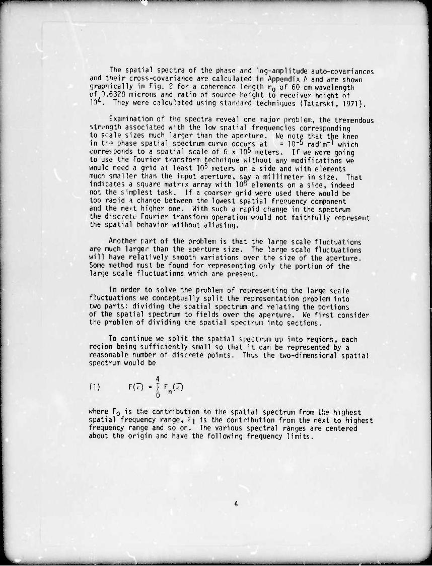
The spatial spectra of the phase and log-amplitude auto-covariances and their cross-covariance are calculated in Appendix A and dre shown graphically in fig, 2 for a coherence length r0 of 60 cm wavelength of 0.6328 microns and ratio of source height to receiver height of ll4. They were calculated using standard techniques (Tatarski, 1971).
Examination of the spectra reveal one major problem, the tremendous strmqth associated with the low spatial frequencies corresponding to scale sizes much larger than the aperture. We note that the knee in th€ phase spatial spectrum curve occurs at ■ 10-5 radm-1 which correvoonds to a spatial scale of 6 x 10^ meters. If we were going to use the Fourier transform technique without any modifications we would reed a grid at least lO5 meters on a side and with elements much smaller than the input aperture, say a millimeter in size. That indicates a square matrix array with 10p' elements on a side, indeed not the amplest task. If a coarser grid were used there would be too rapid ^ change between the lowest spatial freouency component and the ne-t higher one. With such a rapid change in the spectrum the discrett Fourier transform operation would not faithfully represent the spatial behavior without aliasing.
Another fart of the problem is that the large scale fluctuations are much larger than the aperture size. The large scale fluctuations will have relatively smooth variations over the size of the aperture. Some method must be found for representing only the portion of the large scale fluctuations which are present.
In order to solve the problem of representing the large scale fluctuations we conceptually split the representation problem into two parts: dividing the spatial spectrum and relating the portions of the spatial spectrum to fields over the aperture. We first consider the problem of dividing the spatial spectrum into sections.
To continue we split the spatial spectrum up into regions, each region being sufficiently small so that it can be represented by a reasonable number of discrete points. Thus the two-dimensional spatial spectrum would be
(1) F(r) - l F (7) 0 n
where F0 is the contribution to the spatial spectrum from Lhe highest spatial frequency range, F] is the contribution from the next to highest frequency ^ange and so on. The various spectral ranges are centered about the origin and have the following frequency limits.

yTTTTnp-TTTTmpTTTTTTTip TTTTTITTp I lllllll[ | ||||IH[ | |||||||[ | ||||[]|[ | JJlfm I [llllill
to 10 10 ■' in ' ro" lo* IO'1 \on IO1 io2 10 KflFPP (M-')
Fig. 2. Log-log plots of square root of spectra of log-amplitude and phase covariances and of phase-log-amplitude cross covariance.
5
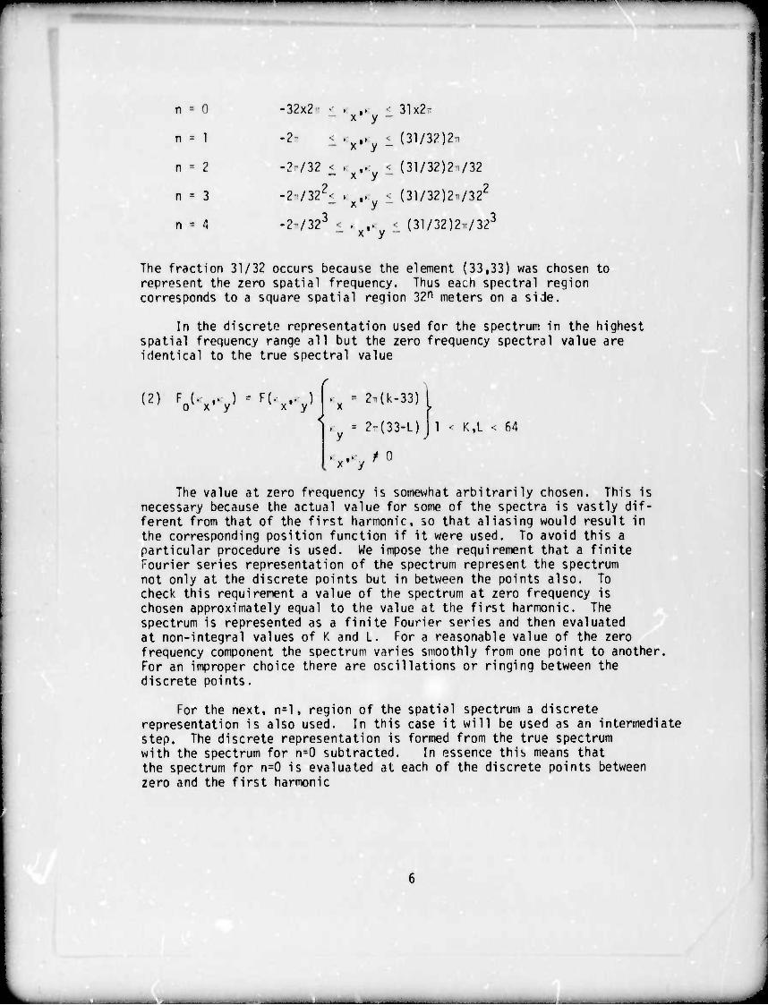
f n ■ n -32x2 ■ .x,.y < 31x2'
n i 1 -2" < 'x.>y < (31/32)2 ■
n - 2 -2-/32 < i ,. < (31/32)2/32 x y
n - 3 -2/3221 . ,. • (31/32)2/322
n ■ 4 -2/323 < - ,. •; (31/32)2-/323
x y
The fraction 31/32 occurs because the element (33,33) was chosen to represent the zero spatial frequency. Thus eacn spectral region corresponds to a square spatial region 32n meters on a side.
In the discrete representation used for the spectrum in the highest spatial frequency range all but the zero frequency spectral value are identical to the true spectral value
w F0(-x-V
F<vV ■ 2-(k-33)
■ 2-(33-L) 1 • Id. < 64
,. / n
The value at zero frequency is somewhat arbitrarily chosen. This is necessary because the actual value for some of the spectra is vastly dif- ferent from that of the first harmonic, so that aliasing would result in the corresponding position function if it were used. To avoid this a particular procedure is used. We impose the requirement that a finite Fourier series representation of the spectrum represent the spectrum not only at the discrete points but in between the points also. To check this requirement a value of the spectrum at zero frequency is chosen approximately equal to the value at the first harmonic. The spectrum is represented as a finite Fourier series and then evaluated at non-integral values of K and L. For a reasonable value of the zero frequency component the spectrum varies smoothly from one point to another. For an improper choice there are oscillations or ringing between the discrete points.
For the next, n=l, region of the spatial spectrum a discrete representation is also used. In this case it will be used as an intermediate step. The discrete representation is formed from the true spectrum with the spectrum for n^O subtracted. In essence this means that the spectrum for n=0 is evaluated at each of the discrete points between zero and the first harmonic
J

(3) <x = 27T(K-33)/32
^ ■ 27T(33-L)/32)/32 1 1 K, L <. 64
and subtracted from the true spectrum at those points. This procedure has the advantage that the newly formed spectrum goes to zero at the JulMl^ SPeCtral re9l0n thus renderin9 * aut?™ ical y Sand-f mited banner ?denrtica^oS?h.Cttral ^ in.the n=1 re9ion is determined n a manner identical to that used in region n=0.
used In'r^?^!!^/0' ^ 0ther SPeCtral re9i0nS iS ident1cal to that
The procedure for generating random arrays over the one meter aperture from the spectra associated with all but the highest soatial frequency spectral region involves a procedure using polynomials This
SUl5 aÄ PreSently- Fl>St t0 f0™ the ^sfsVc^^Jl; aThlS
MCO JUS th- sPftra decomposed as indicated it is a simple matter to use the Fourier transform procedure to generate five sets of random ZfT^ JlfI*f!!2 Siz!S ani t0 find the contribution to an a?2a one ^rt nf^ntL^i^- Center tf the lar9er arrays- 0ne would need so^e sort of nterpolation procedure to go from the discrete arrays to a much smaller grid a meter square. Then the sum of all the contributions
Slre'ct a'pp'roa'ch."16'6' ^ rePreSent the wavef™t- ™« would be tSe
We use an alternative and operationally faster procedure for findina the contributions over the square meter aperture arising from the lower spectral ranges. The procedure as indicated previously is to expand / the contribution to the phase front across the aperture in a series of / polynomials with random coefficients. The variances of the coefficients are determined from the spectra for the given range.
One might envision the procedure as having the following steos Suppose we were to use the Fourier transform procedure to calculated large number of random wavefronts for each of the spectral regions. The wavefront contribution corresponding to the highest frequency spectral range ^retained for use as is. Then suppose we choose a one meter square with 64^ points in the center of all random wavefronts for each of the other spectral ranges. We then interpolate from the large square grids to the one meter square grid. The interpolation should be per- formed assuming that the Fourier series representation for each random manifestation was a continuous one and evaluating it at the 642 points in the central one meter array. Alternatively the sampling theorem could be used for the interpolation. The values at the 642 points for each manifestation would be used to find the coefficients for a polynomial expansion of the manifestation. The coefficients would vary randomly from
■■■Mil

one mamfestation to another. Indeed since the wavefronts vary randomlv with normal distribution and zero mean the polynomial coefficients w? also vary randomly with zero mean. One would find the Sari nJe of St coefficients for each spectral range by averaging the square of »ich coefficient over the set of manifestations. H ^ UT eäcn
Thus one would end up with a polynomial series for each spectral ranae representing the front over the central square meter. The coef^cients of the po ynomials would be norn«lly distributed with zero mean !d own varnnces. To generate another random manifestation one would merely generate a new set of coefficients using standard random number generation llzTul'n Assrn9.^e number of random coefficients required s^esst an 64^ the procedure is quicker.
In the procedure to follow one further step will be added sliahtlv complicat ng the mathematics. That is that polynomi Is w ? be ?o n3 hat will simultaneousl/ represent both phase and log-amplitude. A?so the Fourier transform procedure that is used directly for the highes? spatial
Jotr^Se^^d^Sg^Lp^t^srfV^r"be niodified to »^tÄy^t. In the next section the extension of the basic Fourier transform
rth^PrHn1^1^?0^!^ Ph?se and l09-^Plitude will be con Sed. In the section to follow the polynomial approach used for the lower reg ons of the spatial spectrum will be derived in general terms. regions
3. HIGH SPATIAL FREQUENCY REPRESENTATION
We now describe the procedure used to generate the contribution to the random wavefronts from the highest spatial frequency region. The procedure used is based on the Fourier transform approach but is more general ?he approach is extended to two random fronts, phase and log-amplitude, which are correlated The basic expressions derived here will also be used in the next section in the derivation of the representation for the lower spatial frequency contributions. We assume that the spectra of the phase and log-amplitude covariance functions F^^,^) and F (.x,.v) respectively as well as the spectrum of their cross-c6variance. F K - f JJ1^"*1^« available. W * V
The procedure will be to postulate a particular model and then show that it can be made to have the desired properties. To begin, for a sing'.e manifestation we generate two square matrices. Ri(I,J) and R?(I.J) of statistically independent samples (Hogge, 1974) from a distribution which is gaussian with zero mean and unit variance. Stated mathematically, this
(4) 'V^V^^i.^I.KJ.L

POUulI'e IZttL^^, den0te t,,e «fetation operator. Ue then
(5a) :(K'o-L'0' ■ faf'o^o^fK.L) * Fb(K.o>L.0)R2((;>L)
(5b) ^K.0.L.c)-Fa(K.o.L.0)R,(K,L) + Fb(K.o.L.0)¥K.L) .
Ä fr^'eL", sÄ?t^rthe•?p:ctraheFnT,■", SÜ^ 0f ^
The desired expected values are
(6a)
(6b)
(6^)
<^0.u0)> - <Äi&cotuo)> . fl
(K. ,K. H > 0* 0 •ö2F:(%.L-0)
•^^o^o'^C-'-o-L'o) '^..(^.L.^
(6d) <^(K.o,L.o)2 --2F.(K.o.L.o, .
Wr^rirÄrFa-Fb- a"d ^ «* ^^ (7a) ^% = <h.|2 = v2 ^ RJ^+IFJ^IRJ2- = I« '2. ir ,2
b ^i^1 ,FaK+ IM
(7b)
(7c)
-2 ; v<:*>* = F^!^ 12^,^,2,,^,^ =2
-2 0^ = <m^=|Fcl^|R,|2>t|Fb|2,|R2|2>=,F|2+|F|2,

In Eqs. (7), use has been made of the statistical independence of the matrix elements stated in Eq. (4). Solving Eqs. (7) for Fa, Fb, and F , we obtain (for the case where Fa, Fb and Fc are real),
(8a) Fa ■ -F^ü__
(Ik) F,
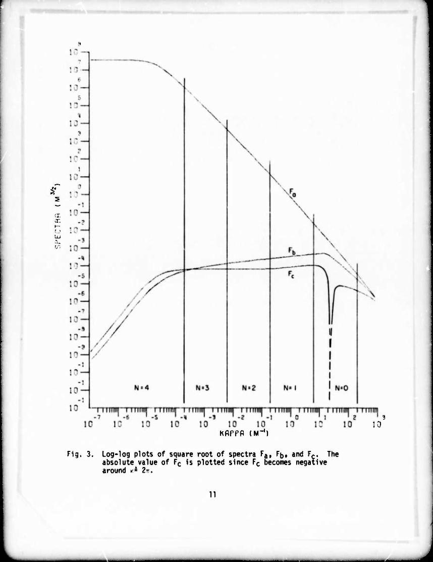
(8c) F = J c 'J^T^l Ihese three spectra are displayed in Fig. 3 for the complete spectrum. Note th^c the magnitude of Fc is plotted since it becomes negative at K
;. 10".
Thus to generate one sample wavefront the procedure is to generate the two random matrices, Ri(K,L) and R2(K,L) and then *(KK0,U0) and ;ftKr0,U0) using Fqs. (5) and then to take the inverse transform using
-,i2TTr(I-1)(K-lHJ-l)(L-in
(9a) No
o'-^o' f
-i2.[(I-lUK-n-(J-l)(L-l)] N
(9b) Ulx0.Jx0) - 'HI Kt<0,l<0) *
Equations (5) and (8) completely describe the desired model for the generation of random wavefronts. The model requires the use of two arrays of random numbers, and three spectra which are nonlinear combinations of phase and log-amplitude and cross covariance power spectra. Wavefronts generated by this model have been demonstrated to have the correct first and second order statistics.
10
a >r t— u
r 10 10 KflPPP (M-1)
13
Fig. 3. Log-log plots of square root of spectra Fai Fb, and F^. The absolute value of Fc is plotted since Fc becomes negative around r* 2v.
n

For the case at hand where the spectra must be divided into regions it is the spectra ra, FK. and Fc which would be divided since it is those spectra from which the random spectra and random wavefronts are generated. Thus the procedure would be to take the spectra in Fig. 3 whKh have been formed from the undivided log-amnl itude. phase and cross spectra of Fig. 2 and apply the spectral divisions, and find the best zero frequency value. Equations (3) {?.) and (9) then give the wavefront manifestations, applicable to any spectral region.
Tn this section we have considered the generalization of the Fourier transform procedure to the case of coupled phase and log- amplTtude. The equations for generation of the combined random fronts have oeen derived. The procedure is applicable to all spectral regions, although U will be used for only the highest frequency region The procedure will be combined with the polynomial approach for*jse in the lower spatial frequency regions in the next section.
4. LOW SPATIAL FREQUENCY REPRESENTATIONS
In this section we consider in detail the representation for the lower frequency regions of the spatial spectrum. The development is based on a polynomial representation and applies to both phase and log-amplitude and their cross correlation.
In the following both the phase and log-amplitude will have polynomial representations. That is, each manifestation of both the phase and log-anplitude will be represented over the input aperture by the polynomial
(10a) .(F) = j .n.n{F)
(lOb) :(r) - I • (?) n
where the .n(r) are a finite set of orthonormal polynomials defined over the input aperture and the coefficients ,n, ^n are gaussian random variables with zero mean and variance yet to be determined. The various random coefficients are in general correlated, cross-* correlations occuring both among the various log-amplitude coefficients and among the various phase coefficients and also occuring between log- amplitude and phase coefficients. The specific form of the individual polynomials for one situation will be shown in the next section. Using Egs. (10) the contribution from the lower spatial frequency ranges then has the form M j
12
J
(Ha) 'I (r) - N y
n=l r r n=l (F).
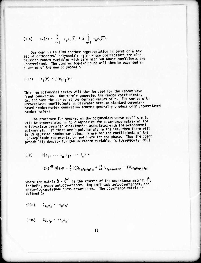
Our goal is to find another representation in terms of a new set of orthonormal polynomials ^(r) whose coefficients are also qaussian random variables with zero Man jut whose coeffcients are uncorrelated. The complex log-amplitude will then be expanded in a series of the new polynomials
(lib) ^(F) - c.^(f)
This new polynomial series will then be used for the random wave- front generation. One merely generates the random coefficients, en, and suns the series at the desired values of r. The series with uncorrelated coefficients is desirable because standard computer- based random number generation schemes generally produce only uncorrelated random numbers.
The procedure for generating the polynomials whose coefficients will be uncorrelated is to diagonalize the covariance matrix of the multivariate gaussian distribution associated with the orthonormal polynomials. If there are N polynomials in the set, then there will be 2N gaussian random variables. N are for the coefficients of the log-amplitude representation and N are for the phase. Thus the joint probability density for the 2N random variables is (Davenport, 1958)
(12) H*v ••• vv ••• i*)
(2-)"N'Q!exp - 1 gQ^gM, + H VnWn + ^Q?n*n,Wm
where the matrix Q = C1 is the inverse of the covariance matrix, Z, including phase autocovariances, log-amplitude autocovanances, and phase-log-amplitude cross-covariances. The covariance matrix is defined by
(13a) •n^m n'm
n3b) c^ - <vm>
13
•MMBaaaaM J

*•»--*•-I—...,,..,.
The calculation of the covariance matrix elements will be discussed later in this section.
The procedure for finding the new random indeoendent coeffi- cients is well known: transform to a new linear combination of coeffi- cients which diagonalizes the quadratic form in the exponent of the joint probability density function. To illustrate this we use a matrix notation. The quadratic form, Q, in the exponent of Eq. (12) is written in vector notation
(14a) 2Q = vT5 v"
where the vector, v, is
« ■
(14b) v= (:r-2 ••• Wv'v '•• S|)
and the matrix ^ is the inverse of the covariance matrix as indicated. To diagonalize the quadratic form find vectors, w, satisfying the matrix eigenvalue^ equation
(15) $ wn = > wn n n n
Then the diagonalizing transformation is the modal matrix, R, whose columns are the orthonormal eigenvectors, W .
n
(16) flT $ A = .f
is the diagonal matrix containing the eigenvalues. Then the new ndom coefficier
(17) 7=Mc
random coefficients c are given by
14

where
(18) c - (c1( ... c2N)
The cn are the desired random independent variables. They are gaussian with zero mean because the »„ and .n are gaussian with zero mean. The cn also have variances rjL given by the diagonalized inverse covariance
The complex log-amplitude in Eq. (11) can be rewritten in terms of the new coefficients. Writing Eq. (11) in terms of a function vector,
(19) *<F) = (•!• -2 ••' -rr J-i« j-2 '•• bj
we have
(20) ^(r) ■ -I(?)v
(21) =-:T(r)Mr
(22) - J(r)c - I znn{r)
where
n n
1T- (23) 5(?) ■ (••■,(?), r2.(r), .... :2n[f)) M1-
Equation (22) is the desired result. The first order complex loq-ampmude, li, is represented as a sum of orthonormal polynomials, the ' (r), with random uncorrelated coefficients, the c . n n
We note some interesting features in this solution. The polynomials 'n(r) are in general complex, since the diagonalizing transformation mixes log-amplitude and phase. The solution is also identical to a solution of the Karhunen-Lofeve problem. This is demonstrated in Appendix B.
15

' """•■■
We pow proceed to derive a general exores^inn for thQ ^ matrix C from which its inverse Ö = c-lrSnhn nhtl- ^ e "va!:1ance
vation involves a severa step procedure Bas^a "fhp .Hi deri- to conceptually generating a SavTron^which ^t a% ^^T"' .sing the Fourier transform technique. The stat^tica p?opert es of this large wavefront are thus known from the proceeding sict on Next imagine that we generate an ensemble of wavefrSnts and fntlr polate between the matrix of points using the Lmpl?nq theorem representation. Imagine that we then take the cene? one square meter of each ensemble member and expand that in terms Sf S?2l«
fhe arnHPreSe;tati0n.0f EqS- (10)' We can ^ detTJne e^ch of' cSv ances ' T> ^^ T^ *"* further can ^e^l
rfUntZnfHa ■,"'?'' l:rVn:' and cross covariances, <,n<,m> con- stituting the elements of the covariance matrix. In Eqs MOl ■(r) and :(r) are defined over a one square meter aperture Usinn the orthonormality assumed for the polynomiair n(r-) we can »Hto
(24) ••n = |j-(r) -pCr) w(r)dr
where w(r) is the aperture function,
« (25) w(f) = 1 J • V2 < X < 1/2
j- 1/«<y < 1/2 .
0 otherwise .
in Eqs. (7) We thintSTJhl :lK>0•L>o, anJ (K^o.^o) as indicated over^heWge array ' 1n'erSe transfo™1 ^ obtain the phase
P jir((K-l)(M-l) + {L-l)(N-l) (26) K%^) - KJ IWfcc^), o
16
^

—w-«——■—-W^-^WBIIH
■ Mi I -m
(27) :(x.y) ■ )' I :(Mx .Nxjsinc M N 0 ü
r. L o
(M-33) sine;' L-- (33-N) LX0
where sinc(u) sin(u)/u. Combining Eqs. (5), (24), (26) and (27) gives
where
(29a) Un(K.olL>o) n I J VjMx .Nx )e 0 o || |j nv o' o'
%((K-1)(M-1)+(L-1)(N-1))
and
(29b) Vn(Mxo.Nxo) =j|dr w(r).n(f)si nc-r — - (M-33) sincTT S- - (33-N)
A similar expression can be derived for the log-amplitude coefficients.
(29c) 'n " I pc^O^o^l^O^^^b^O^O^VS^O^H^t^^
The covariance matrix elements then follow from Eqs. (13), (28), and (29).
(30a) C, 'n'n
' ' ^n.L J|2*!Fb(fe0,Ua|2) U;(kKo,Uo) nTm K L a o' o'
[in^o-o)
I I 'I2* (K^»L^)Um(K^.L^)Un(K^.L<„) pro o o m c o n o o
17
~. ^^ .
ftm^im wmimmtmr
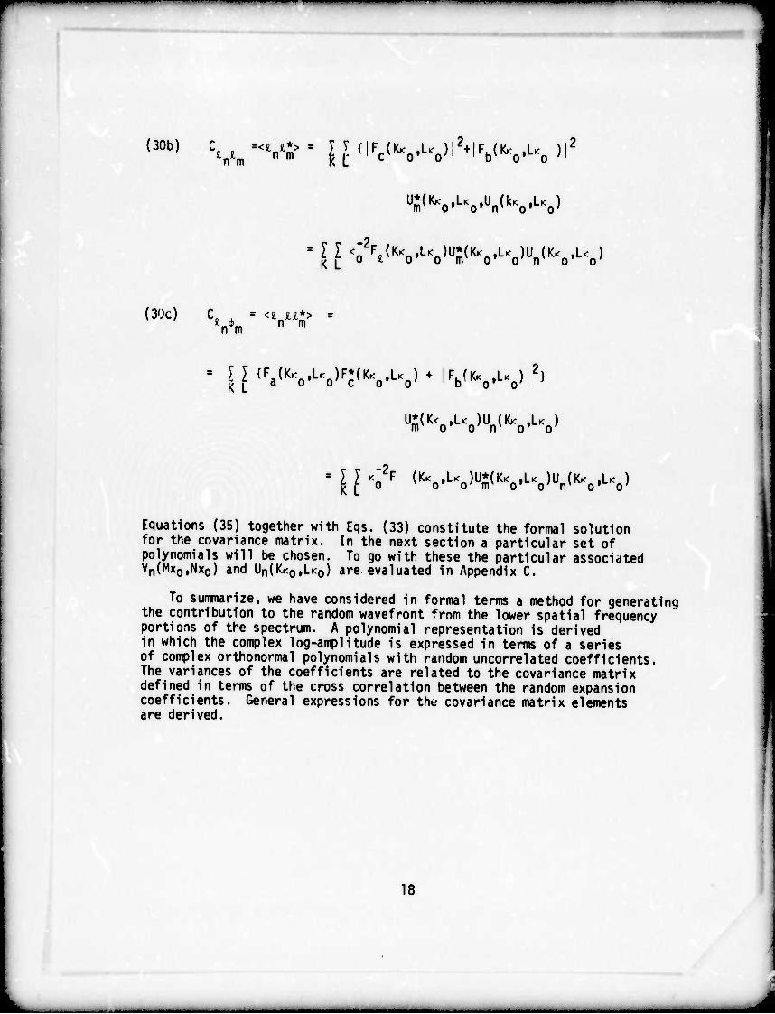
(30b) CVm=<'"*= ^''^^o'S'l^lV^^o»
mx o' o* rr o' o'
{ [ Ä(S'Uo>U;<KVUo)Un<KVUo)
{3üc) C. , = <in*> = n m
ll{F^o>UoK^o'Uo)+ lVS'Lgi2}
m' o o nv o* o
= 11 K L
-2t KoF ^o'UoK^o'l*o)[i^o'1^
Equations (35) together with Eqs. (33) constitute the formal solution for the covariance matrix. In the next section a particular set of polynomials will be chosen. To go with these the particular associated Vn(Mx0,Nx0) and Un(K<0,U0) are-evaluated in Appendix C.
To summarize, we have considered in formal terms a method for generating the contribution to the random wavefront from the lower spatial frequency portions of the spectrum. A polynomial representation is derived in which the complex log-amplitude is expressed in terms of a series of complex orthonormal polynomials with random uncorrelated coefficients. The variances of the coefficients are related to the covariance matrix defined in terms of the cross correlation between the random expansion coefficients. General expressions for the covariance matrix elements are derived.
18
ngppviw^^w
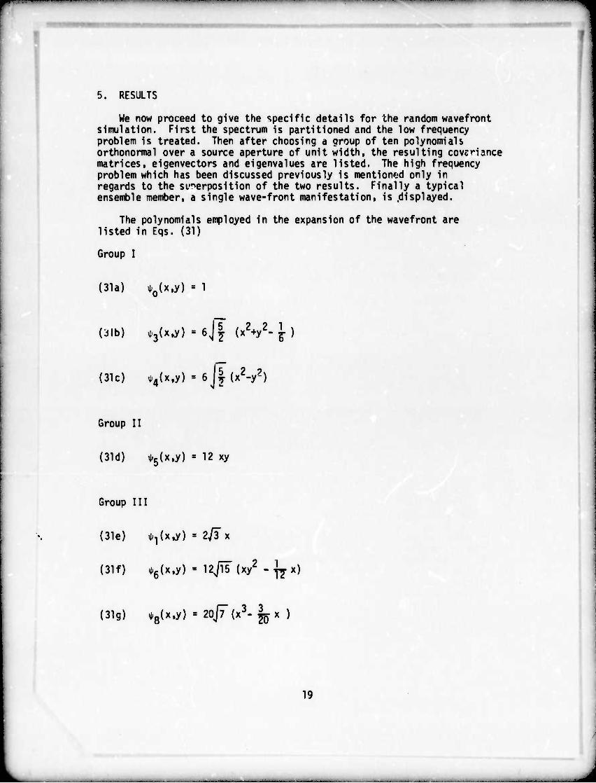
5. RESULTS
We now proceed to give the specific details for the random wavefront simulation. First the spectrum is partitioned and the low frequency problem is treated. Then after choosing a group of ten polynomials orthonormal over a source aperture of unit width, the resulting coveriance matrices, eigenvectors and eigenvalues are listed. The high frequency problem which has been discussed previously is mentioned only in regards to the st-^erposition of the two results. Finally a typical ensemble member, a single wave-front manifestation, is .displayed.
The polynomials employed in the expansion of the wavefront are listed in Eqs. (31)
Group I
(31a) *0(x,y) ■ 1
(31b) ^(/.y) = |j| (XV-^)
(31c) ^(x,y) ■ 6j|(x2-y2)
Group II
(31d) ^5(x,y) ■ 12 xy
Group III
(31e) ^(x,y) = Zjlx
(31f) *6(x,y) = IzJlMxy2 - ^ x)
(31g) ^8(x.y) ■ 20j7(x3-|&x )
19

■■ ii i ■ 11 ■«nqppmtiMwwHm
Group IV
(31h) ,2(x.y) - 2jly
(311) -/x.y) = 12^15 (yx2 _ 1 T7 y)
(31J) ^(x.y) - 20/7 (y3 - ^ y)
As indicated the polynomials are chosen to be orthonorrral over a umt square as described by Eq. (25). uruionorrai over a
The grouping of the polynomials in Eqs. (31) was done to indicate the s^ilanties in symmetry. The first setV0r).o(?) and d R employ the same combinations used by Fried (1965) T^ey are even
Jhird JJ ?.nd ^H ^ Se.COnd Set' '5(rl is odd in both x and y The SP ar nlnt?^!1"-^^ even lnuy' The Poly^ials in the fourth set are TdentTcal with tnose in the third set except for a ninety nfth! TSPÜl' JS o"*™^ exPect the statistical properties of the last two sets will be identical because the correlation functions and power spectra have central symmetry. '«"www
nf fh^ IS! lUpJfimrym choice of Polynomials is the partitioning of the spectra. We used a trial and error procedure to choose new
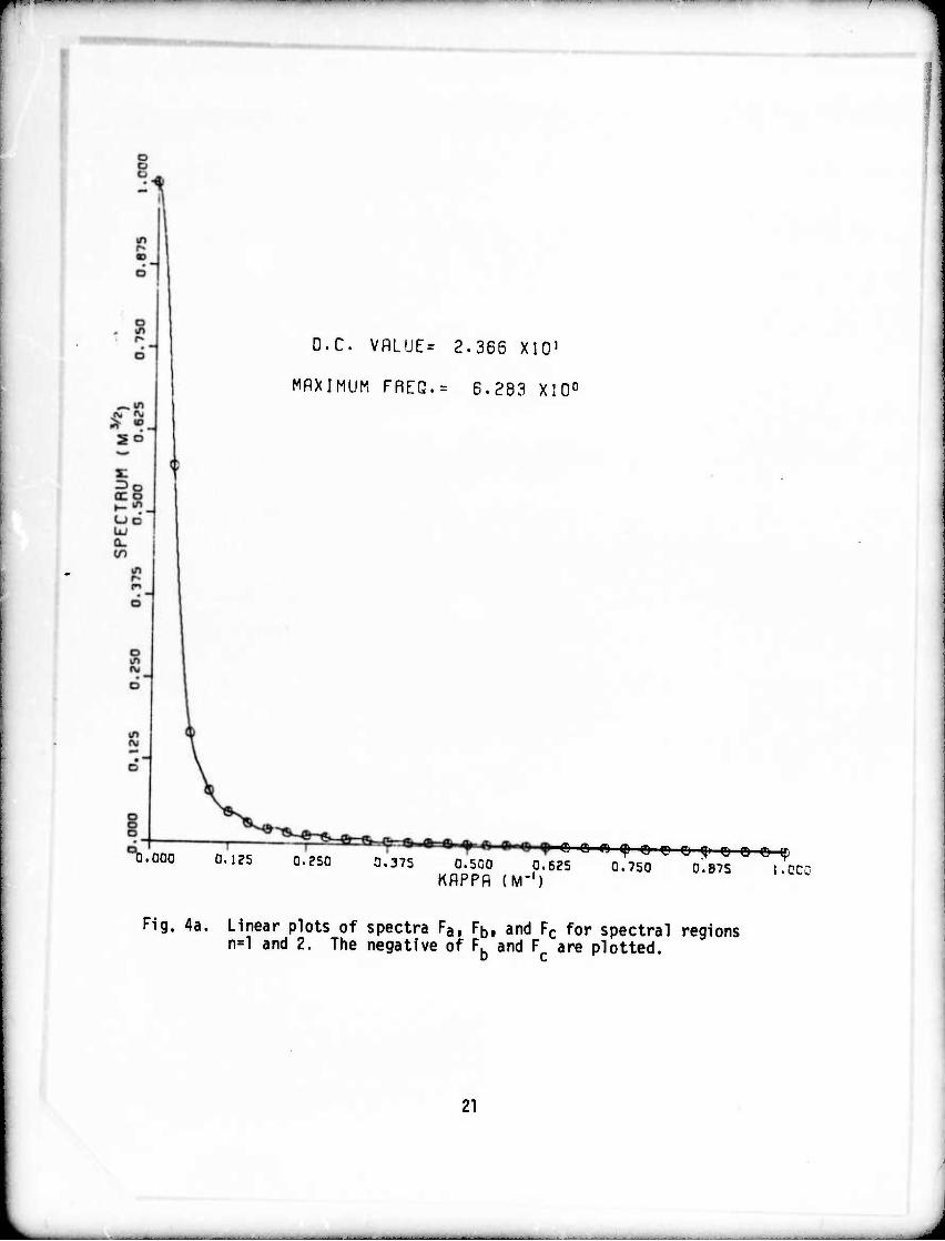
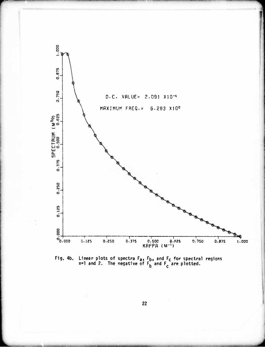
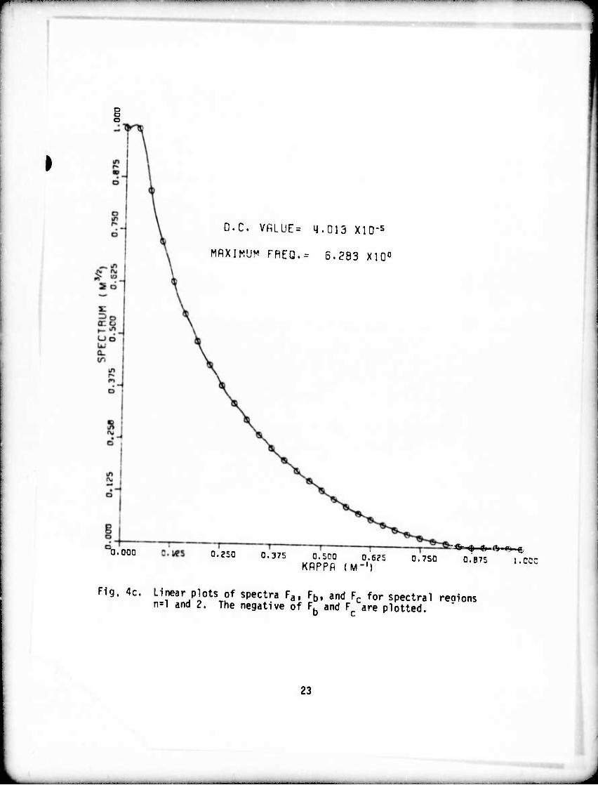
eaL 'Fnr'F V? p^ f0r/d' Fb' ^^^ in the hi5hest sP^ial frequency region For Fa the zero frequency value chosen was 1.75 times the value for the first harmonic. For Fb and Fc the zero-frequency values nfrfhleiefqfUal t0 the Values of the ^spective first haJnics p\otl I rLli T™ TCtJa [!Sed for regions ' and 2 are shown in Figs. 4 The circles indicate the values at the discrete points while the solid curve comes from the interpolated values. The last curve is an example of a poorly chosen zero frequency value.
The next step is the generation of the covariance matrix. There is a simplification that arises in the covariance matrix because rln h! ^-^ Properties of the particular set of polynomials which can be most easily demonstrated by choosing a particular order for the polynomials. Thus for the function vecton,'(f) in Eq (19) we choose a complex twenty element vector H. v / we
20
- ■— ■- _j
B| '. ' ■ ".'
O.C. VflLÜE> 2.366 XIO1
MAXIMUM FREG.= 6.283 XIO0
0.000 0.125 0.250 0.375 0.500 0.625 0.750 0.875 1.000 KflPPfl (M-1)
Fig. 4a. Linear plots of spectra Fa, tbt and Fc for spectral regions n=l and 2. The negative of Fb and F are plotted.
21
f
0.000
D.C VflLUE= 2.091 XIO-1*
MAXIMUM FREQ.r 6.2B3 X10c
IE5 0.250 -i r
0.375 0.500 0.P25 KflPPR (M-')
0.750 0.875 t.000
Fig. 4b, Linear plots of spectra Fai Ft,, and Fc for spectral regions n=l and 2. The negative of F. and F are plotted.
22
»
g
O.OOC
D.C. VALUE- 11.013 XlO"5
MAXIMUM rHEQ.= 6.283 X100
C.2S0 0.3V5 0.500 0.6P5 KflPPft (M-1)
0.750 ff»- q) g. <lj Pi g
0.875 I.OQQ
Fig. 4c. Linear plots of spectra Fa, Fb, and Fc for spectral reaions n=l and 2. The negative of Fb and F are plotted.
23
J


m^^
a'
?
aE8
L')
§
JJ / \
□
in
ti
D.C. VALUC« 3.•167 >l0-b
HflXIHUH FfltQ.» 1.953 m.i
\
\
\
X \
\
^
^
\
[i , n I1.000 o.;?5 0:no „T;,, 0;5cc
\
\ 1
0.625 0.750 O.BVS i • KflPPfl (M-1) 0,8/s '•
^ig. 4f. Linear plots of soertra F Fu an/4 c * n-i ILi • »J spectra ria ht), and Fc for spectra n-1 and 2. The negative of Fb and Fc are plotted. 1 regions
26

(32) ;(r) (V^^J^^^^^) Jv, (r)(j.6(r) .j;8(^).
J.2(r).j;7(F).j.9(r)..o(F)l.3(r),.4(r),.5(r).
•1(r)..6(r)..R(r)..2(r)..7(r),.9(r)).
[he resSus^ ^ ^ ^'^ firSt f0r later con^nience in displaying
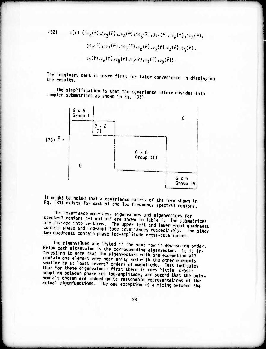
.imnw '7p1;f1cation is that the covariance matrix divides into simpler submatnces as shown in Eq. (33).
6x6 Group I
(33) C
2x2 II
0
6 x 6 Group III
6x6 Group IV
It might be notea that a covariance matrix of the form shown in Eq. (33) exists for each of the low frequency spectral regions?
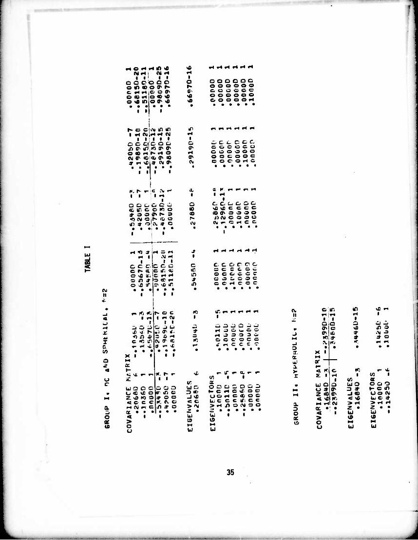
sDPr^i'ranw" ^l^ 1 ^W*^ ** eigenvectors for spectra reg ons n=l and n=2 are shown in Table I. The submatrices are divided into sections. The upper left and lowpr right ä^adrants contain phase and log-amplitude covariances respective y The other
two quadrants contain phase-log-amplitude cross-covariances.
The eigenvalues are listed in the next row in decreasing order Below each eigenvalue is the corresponding eigenvector It is in-' teres ing to note that the eigenvectors with ?ne excepetiin 1 contain one element very near unity and with the other elements
HI E Lai le-St Seyeral orders of ^gnitude. This indicates that for these eigenvalues: first there is very little cross- coupling between phase and log-amplitude, and second that the poly- nomia s chosen are indeed quite reasonable representations of the actual eigenfunctions. The one exception is a mixing between the
28
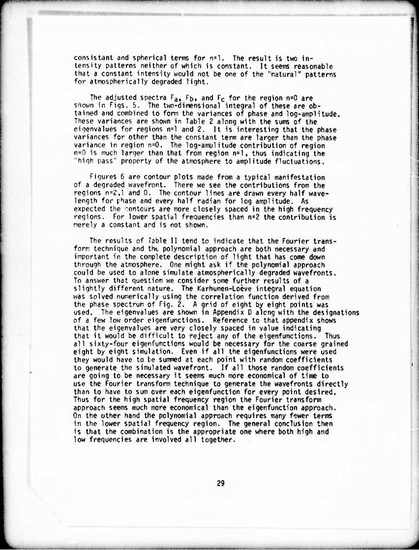
■■ 1 consistant and spherical terms for n=l. The result is two in- tensity patterns neither of which is constant. It seems reasonable that a constant intensity would not be one of the "natural" patterns for atmospherically degraded light.
The adjusted spectra Fai Fb, and Fc for the region n=0 are shown in Figs. 5. The two-dimensional integral of these are ob- tained and combined to form the variances of phase and log-amplitude. These variances are shown in Table 2 along with the sums of the eigenvalues for regions n=l and 2. It is interesting that the phase variances for other than the constant term are larger than the phase variance in region n=0. The log-amolitude contribution of region n=r) is much larger than that from region n=l, thus indicating the high pass" property of the atmosphere to amplitude fluctuations.
Figures 6 are contour plots made from a typical manifestation of a degraded wavefront. There we see the contributions from the regions n=L,l and 0. The contour lines are drawn every half wave- length for phase and every half radian for log amplitude. As expected the contours are more closely spaced in the high frequency regions. For lower spatial frequencies than n=2 the contribution is merely a constant and is not shown.
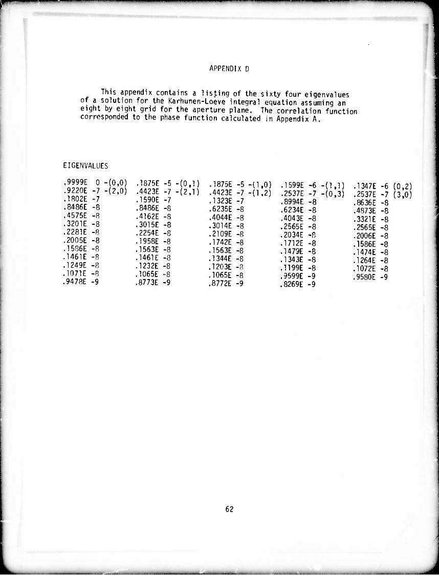
The results of Table II tend to indicate that the Fourier trans- form technique and tht polynomial approach are both necessary and important in the complete description of light that has come down through the atmosphere. One might ask if the polynomial approach could be used to alone simulate atmospherically degraded wavefronts. To answer that question we consider some further results of a slightly different nature. The Karhunen-Loeve integral equation v/as solved numerically using the correlation function derived from the phase spectrum of Fig. 2. A grid of eight by eight points was used. The eigenvalues are shown in Appendix D along with the designations of a few low order eigenfunctions. Reference to that appendix shows that the eigenvalues are very closely spaced in value indicating that it would be difficult to reject any of the eigenfunctions. Thus all sixty-four eigenfunctions would be necessary for the coarse grained eight by eight simulation. Even if all the eigenfunctions were used they would have to be summed at each point with random coefficients to generate the simulated wavefront. If all those random coefficients are going to be necessary it seems much more economical of time to use the Fourier transform technique to generate the wavefronts directly than to have to sum over each eigenfunction for every point desired. Thus for the high spatial frequency region the Fourier transform approach seems much more economical than the eigenfunction approach. On the other hand the polynomial approach requires many fewer terms in the lower spatial frequency region. The general conclusion then is that the combination is the appropriate one where both high and low frequencies are involved all together.
29
J

g
p
O in r-
C
^ß I in ^ J
Id]
n.c. vp'ijf.- 1.32, xl0-?
MHXIML^ r«CQ.« 5. en X1C?
- o H8IJ UO 1 UJ
di \
o o o
0.000
KflPPfl (M-1) 0.875 1.0
Pig. 5a. Linear plots of soectra F F. »^ c . .
region nP=0. TheSS,ra
tu;rofbFan?s^öued:n the SPeCtra'
30
■M^Mt-M


"•^■w m^m*~m^^^^^~m
■■y\ r
?
rv. in
« to
5d
D.C, Vfll Uf- 1. 106 XlO-11
MRXJMUM FREC.« 2.011 MO'
cc o
Ud UJ
CO
in p
tM
in ' r. i
o o D -T
jr 6*4* # ^ <u , 't-(^-<5-^.
• ■• -^-^-^ ä •?». -<^ ^v~»v. *ir v ?'' ■»
o.oan o.i?5 o.?5c ^•373 0.5?n c.6?5 Kfif f'H (M "')
0.750 hits
Fig. 5c. Linear plots of spectra Fa, Fb and Fc used in the spectral region n=0. The magnitudi of F is plotted. spectral
32

Wi»
1
•H IT 4) r4 r> S •-< I »HI I I
O O O - Q O O O ffv C \X) (V C vC cj <^ y rr, c. m io o 10 10 o »n »n o * K) • ••■••
i i i
IT >£ tt, t^ <i, t- • t t-l I I rt
I I C C 12 C C L C- i» O ö h- >£ U) O ^) uJ vfl iT- * ^ IT f» m fO « Vt Kj «H kC 7
I
to
o c c c c c O O O C O 3 c c r*- o o o o o >o o o o O O sO C O »4
& v£ ^ ^ r^ ^ rl 1 1 • 1
c^ c c c c c c r- c c o m c o >-M O K) O K> 3 o m C If) O (T o o M " vl, O Og i-( C
I I I
"• u »• A fte M II i I
t_ C C C. C. Li •o <r c «i c c. in o a «n Q o ^ «o o r^ ^ c c\ ^ c «i r^ c.
•u U. T *- »l n ^< 1 1 1
Cl £■< Crf ^_ i—t i__i C_> tt a 0 c, c c e »H J» CO o o o o f^ Ji J' t o o J r- m « c P« c e
I
«H ^ « X; •H I tH I I
I
c c c o .r t-i C vfi CM
c c c w o a- C vC Oi
O >-W »C 3 i/J -O c in n O «O X)
• • • I I
(N. I
A,
-f)
3- I
c c c c c c o e c c. c o O O 1= C O f^ i. 3 3 O O ^ O C rt C- O si/
II 2
< u
0
I
C CV, rt iT v£ U I t-l • I rt
I I 3 - C »J C .J rs» c ^) (r m s J* x & u z. L IT. I/". ^, t tH if, •-I (T J- ^ \£ K- • •••••
XI I II
< ^ c; *- <. tt ^ ■ i i u c c c 2 o a U O) CN. O O (T C iT rt (T. C ;f) «£, O « if if e N a. c rt IT rt o rv * c X • • • • • • < I I > o u
<V< (V rt rt m ^ rt I I 11
^ C L> _ C JJ CJ rt IT O 3 0 tf' o Vi •£( 3 ^ 4; -O w rt C C C. ^ J1 C c -v rt r * ^ c • ••••••
I
^ r- C .- tt r* »- 0^ I ||
to ir
_J rt UOt&OCvCO «u. L. c a, c a a c z • <:•••••• L, Uli (A o rt rt
sfi CL m * rt 1 1 i I
a o a a a A. .A. o O 3 3 ^ 3- »H J tv O o rt C r«- r- r- vi t- • • • • • o • • • • • ff X I
a: rt Ui 1 a ^- >- < r- \t »-■ »- a r i. 1 1 1 (/> 1 • w ■
U 3 o UJ a O Ci o rt u cr cy 3 (T 1- C C »-I •^ K o _i r«- U O rt
« rt <v « t- Lj C -. a •-« rt r^ ^ rt > rt X 3 (T • • z • 2 • • O < 1 UJ U 1 a: > u» o o O ►^ ►H
u u kl
33
^^^^^M i^ta^^^MM

«A N r- « 0\ (T • I i i I I
o o o o o c ^ If . X) »-• rt j- 9 C IC 3 3 n o (o !>» h- (r> 4) »♦> »^ ev c^ <^ * • •••••
• • i
^ *> sO * w* ** O * I I I I I
o o o o c o o ") m (v >i) o^ \c o If) •■* 0 N CL IV »x. •^ o tO w) h> « o^ ■1 cv e (v <o «H a * ••••••
i i
vfi u, r^ co r^ a • ••ill
c* c c t: c c * * IC tTi sß r* r- <a o r^ a> ^ m (M K> Oi \A (r <v •- ** e^ »-I t\( • •••••
i i i
^ «f ' * 3 O O >£ • * I I ^
o c C c c- c c P (V> 0 fC (\i f-i 0 ^ «0 rO 0J O f» r«- vO »H O »0 vO « K)
• •■•■•• i
«i VL h- a a • I I i i
LJ Ci O l_i o u 0s »-I (T IT If, r^ o r» *• r» r«- * O tT & 3 c\i N «- <\ "C •«, CN. C\, ••••••
• I I
£ * if w, t C ^ • III |
CJ CI O C CJ C C -■* (T r-i CV <V vf ;»■ 3 "O <fl * «O ^ 3 2 Ai ^ 3 . j> .n ^
* •••••• • i ii
.\ »c -o vc r^ r» •<i • ••ii I 1 ^-
II 2
c c c> c c c c c ^ if . a in l*i <c ^ f) » » c >r f^. « If. <i w <) K o
U * (\ * o ^ 'S/ •0 • a • i 1
Ci
CJ C\. w* K. \l \C N p»
• 1 1 1 1 1 1
CJ ^ zi ^i ^ - 3 X «o c- ^ ^ , \l: Oj «I x» r» m -^ t 2 fo t4_' C O iT ^T (\| K c — ^ r- ^ -^ ^. ^
• _J X
•-< • 1 1
» CC
•x »1 = «J * 4 II III
o c c ore «fJ IT r» \£ a' c ■e c a \, N <v ■o r^ c> j- p» o •^ r^ (T J- ^i x ••••••
I I I
ri C 11 ^ ^ y^ • I I I I
•f K y> j> X /, J^ J> ^ f^ 4: r^ x c vc M t-i r^ r- y p> «>. »• |k • •••••
1 1
* • c (w A in ^ a • s: 1 1 1 1 1
5 UJOCJCUQCP N 0 * K) e y ,H e«,
2 >A % 0> o ^ ^ «f- <tr>ccccirc 3 a: • • • • * . s < • • • u o
Q
c *■ »^ f 3 if ^ M 1 1 1 1 1
1/) or -JC OCQOQOC
-JsO U CT sfc rl <\| r-l 0^ <if L-a^vto^iet-i >(\) > J\ -t ,-1 -o .-< -, pr • ^ • • • • « • UJ D II,
34
M^^MMMWk
«* o t-i fi in 4) « (U»4: Ol ^
1 Q
II1 II Q O C O O O o o a o a c o m <o o ff^ ^> 1^ O O o o o o
C «4 r4 O O ^ G C (2 O O C C
O (U *^ o «o \0 M> o o o o o o
o \a in o «r vfi s O O O O O tH
• • • • • • • i • i
1- o c »\» ir< ifi & I «H <M r4f-l <M ft
1 1 i i 1 1
a c a'c Q ci o ^ C C C C C- Xi (T U"i;iO IT (T 0^ o o c o c o O tf> t-l ^ r4 O H o o o o o o (VI IT C Oi (T CO <r o o c o o c & r* \C ■ 9 CM (T (V O O C O t-t c
I I
«. ^ vttl .>, ^ i a 1« r* v r* T*
11 1 «4 1 1 »H | 1
O O t- C* C »J o C C U O O Ci
CL IT C. C IC O « vC vfi C C C C * o o a* r*- 3 CO CO 0^ 3 o o o
•O tx O.l» <i O r»- J) CV c o o o tfl * o'cv * c kM CM «- C: «^ C C
.••!••• • 1 1 1
•
*m mm»** J- ^ l\ M* 1
1 •• C C C IC c c C c c o c re & f^ a c ir. a. ir C C = C O w
e sD U. 'C r^ iH un o c o c c c ^i J> ^ ta <E »- * C O i o o c O ^> IT r> »ir <r r» c c »^ c c: c
Cü . . • • . • • II I i i ^ | • 1
CM II
C IT. If) vC W* mi r* K; K, N O C (O
1 r^ ;r< ft 1 « 1 r^ 1 rt CM i 1 1 1
1 Q O «)
1 1 ■^
M WJ a ^i a J -j t-i ^ O w w O ^ J 3 O 3 w o o c- o c c
_ a o
c 3 3 Ö Ml
I <) o a c f. \r- »- •-' «i • . •
■ti cr a. = O -H CV (T oc
• . • •
J
i en K)
. X 1
•f * o
X 1 1 i i a I-«
5 at ^ or —
« •- v. \i. r- T-> K. f •- s£ »- vT •- a. f •-
C/l 1 1 a O D CJ Z, D O _l t- C t-« C sf o C OO tH C «I O C; U. c C C If c c > ^ /j o CM a o 2 • • • • • • Ul 1 1 (9
y
>- r SL 1
C. •H
tc I M 1
•
£.
Ui O O Ci O * vC o z. vO to o < c c c i-i CM tn O x • • •
1 1
Ci o o a iT« Ci » o o If. CV. c .0*0 . . •
-Ivfi « c > rvi 2 •
•
•-•
UJ o o * 2 «O < vC
X • 2
1 a
CM • ■
(A uj o 3 * -1 (0
> fl 2 •
a O O O ►- c in UO CM u, c * > fl H 2 • • U 1
o < 1 1 U ^ > 9 CD
s 8 u o o
o M U y
J

»4 * * * 9* V* O« r4 r4 r* r-t r4 r* v4 I I I I I I I
O OO O O O Q ^ O « t-« tO \A J) r- in *-> a.. 3 st> <£ (0 O « tO <0 r4 ri sD K) rt (T ^ (M (M • ••••• •
I I I
o cocao CO o c o o CO c c c c o o o o o o CO O C O fl • • • • • •
c (\, » m r^ a> 1 1 1 1 1 1 1 O <- O (_ ^ c c o a r _ c J (r> <i> c if) <c if. (0 2 O o o o o f«. «O Ifl o ^ * (J^ =>o o o o o O «H C \0 h> <c r^ o o c c c o H r- T r^ ^ * t-i c c C C fH c
I I I
r^ & witk if u.
I
1 t-l iH •H *4 ft f» 1 ri ft 1 1 . 1 1 1 1 1 1
c Ciulc a a Ci O C C- C C C * a * r^ m « CM CV « 3 c c c ■o r» r-« .3 « A r^ « «H o o o o a <o|<-> >c if) ft OJ if) r o o o ^ ^ w^> •■« cr r^ K) n r^ ti c c
• i ii 1 1
II 2 » r^ c .-i * ^ jj » r^ C fl fl fl
1 1 l.rl -1 c-l i 1 1 • III
u C DC C c: C o o c c c c c ►-■ ^ K; K>,* C C. ® r. ^ cd c c o C. r«. c- Mt* r. K; c. v£ f^ ^ C C = 3 a> w « I u -J * \< /) f a> o o o •o ,r, -< r-vL <J ^ ■r. fT <V 0" CCO
• C i i i 1 J. ; «r
i * «i i^ t ft. 3- vL * O fl »- f« r« <r i i i r^ »^ r^ 1 1 1 ^J 1 1 1 -^ Q Ct J al ^ «■! o a c*o j d s tm - \i "O tf\ -i O t^ IT 4; 3 C 2 O -t & U J* r»- -o J) n i j\ r-- o o o
vf 0> O c »- c <r fl (T fl c o o • ; «. •-• »- f IC .-■ 3 !T ft, ^ c c
> • • • • • • • •- X 1
1-4 1 1
C ae ■» ^ «- « f d d !>■ C r- f f d * h- f« fi • t" I 1 1 F^ r^ LO III
M 1 1 M (T «- UJO oo C Q Q Ul o o D o o c a o w U vO r- K) » (T * O sT ►- O C- ftl ft( c o
2 lO C> N IO t^ r»- _J »O u o a< m r» o o t/^ « vt vt IT »O C tt C M. L. C C \i «, C C 1 >-• fi X D <£ »H >c > f« > tH * K) -O C O 3 ac • • • • • • 2 • 2 • • • • • • o 4 1 1 1 U U III
s > (fi (A O ft •-1
o LJ u

I
Fig. 6a. Contour plots of the contributions from spectral regions n=0, 1, and 2 to phase front and log-amplitude front.
37

Fig, 6b. Contour plots of the contributions from spectral regions n=0, 1, and 2 to phase front and log-amplitude f^ont.
38

1 ' P^^W-^^^^P»^^-^»^^^»^^I »-«•
Fig. 6c. Contour plots of the contributions from spectral regions n=0, 1, and 2 to phase front and log-amplituoe front.
39
y

r ■' ^^m^^^mm^^
Fig. 6d. Contour plots of the contributions from spectral regions n^Q, 1, and 2 to phase front and log-amplitude front.
40
——-—.^aSA^—M.. ___^^^

^^^m^mmm^B^-TM
Fig. 6e. Contour plots of the contributions from spectral regions n=0, 1, and 2 to phase front and log-amplitude front.
41
M^HU^-.

Fig. 6f, Contour plots of the contributions from spectral regions n=0, 1, and 2 to phase front and log-amplitude front.
42
- ^

TABLE II
n Variance Phase Log-amplitude
0 .2220 ^ .3017xl0'3
1 .5543xl02 .9330xl0"6
2 .2068xl06 .2788xlO"R
One other item might be mentioned in passing. In the ■MlltaH*.
that way and perhaps always will, fhe method of relatnq the usual requirement for pc.itive dtflnlttMSt. that aM the sub determinan <;
on fMs^oint10 ^ SPeCtra iS ^ 0fc— Mo- ^cM'SS
.ni HH^lli alier ^e new sPectra have been computed for reqion n=0 ani the eigenfunctions and eigenvalues have been obtained ?or?e3ions n-1 ... C we can actually generate the random wavefronts This ?s
(22") TnrVSV {S) ^M f0r the highest Vectra! re ion a 5 q 22) for the lower spectral regions. The procedure is illustrated* in the computer algorithm shown in Fig. 7. musirated
sdJS srfnSt^fL'Js1?: ^ comp:eie wavefront ****** .tnerie was illustrated for the spectra under consideration A set of polynomials was chosen for the low frequency spectra reoions and the covariance matrix diagonalized to give\ e Karh neSSeve polynomals appropriate for uncorrelated random coefficient A complete wave-front was illustrated in terms of the contHbutions from the various spectral regions. tomriDuiions
6. SUMMARY
ripnrllnT^v^V e ha-e ?e^l0Ped a scheme for simulating randomly fdJft*PKCa2 •eamS 1ncluding both phase and log-amplitSde and y
the effect of their cross-correlation. The scheme works for optical degradations whose scale lengths range from much smaller to much larger than the input aperture size. An extension of the well-known Fourier transform method is used for the small scale fluctuations and a polynomial approach is used for the larger scale fluctuations.
43

r, 0
m( • • • m\
.0_ N-4
RANDOM ARRAY
N-0
RANDOM ARRAY
R2
i.OG-AMP £
LOW FREQUENCY
HIGH FREQUENCY
PHASE
LOG-AMP JL
COMPLEX PHASE
F-g. 7. Schematic diagram of computer wavefront generation algorithm.
44


r
During the process of developing this wavefront simulation algorithm several other problems were solved. The problem of using the Fourier transform method to simulate both phase and log-amplitude fluctuations includino their cmss-correlation was solved. The problem of using the Karhunen-Loeve approach for wavefront simulation was considered and extended to a complex variable, the complex log-amplitude, thus enabling the application of that approach to both phase and loq-amplitude, A problem of handling the large range of spatial scale sizes was solved by the spatial frequency division. Further the problem was solved using an efficient scheme by combining the Fourier transform approach and the polynomial approach or ranges where they can be most suitably used. This technique will be especially useful in the computer examination of active systems to be used for the compensation of atmospheric degradation of images (satellite, etc.) the light for which has propagated large distances down through the atmosphere.
46
j

APPENDIX A SPrCTRA
In this appendix we derive the expressions for the spatial spectra of phase and loq-amplitude covariances and the phase-loq amplitude cross covariance for light that has propagated down throunh the atmosphere. The expressions draw upon work in the literature (Tatarski, 1971) and end up with computer evaluation of the associated integral expressions. In this case the spectra are particularly sig- nificant because they apply to a light beam which has propagated down throunh the atmosphere where there is a much larger low spatial fre- quency content than for light propagated horizontally near the ground,
The starting point for the three spectra are expressions in the literature (Tatarski, 1971, Fqs. 5-27, 5-33, 46-14,15,16, and 46-22, 23,25,26).
(la) F^.L) - k' -L -L j^d'-z")
exp ; o- 0
2 k F^k^z'-z-^'dz"
(lb) F2(.-T,L) = -kL -L-L -i ^(PL-z'-z")
exp — o-o
2 k F (-.z'-z'^dz'dz"
(lc) F 7Lrl [F, ♦ Re(FJ]
(Id) F - \ [F1 - Re(F2)]
fie) F - y Im r2
(If) B/:) - 2 J0(-r )F|(.TIL).Td.T
•' 0
47
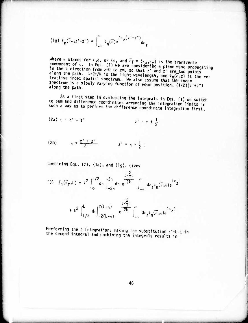
n«) y^-i-j = _ jtc-d'-i«)
along the path, -^/k is the light wavelength, and :n(r z) is ?he re- fract ve index spatial spectrum. We also uimi that the index
afongthe^ath ' Varyin9 ^^ 0f ^ POSition' (V2)(z'+z")
t. c AS L^Ri Step in evaluating the integrals in Eqs. (1) we switch to sum and deference coordinates arranging the integration limits in such a way as to perform the difference coordinate inJegraJionfirs^
(2a) • ♦*
(2b) n = z' + z" I
Combining Eqs. (?), (la), and (lg). qi ves
(3) F^.L) - k; fL/2 r2fi
dn e I z n
+ k" dn '1/2
2(1-,)
-2(1-0
J>r
i V«^")«V
thlfc^ln3 P1! \ ^^^tion, making the substitution n^L-r in the second integral and combining the integrals results in
48

(4a) F^.^L) 2 |L/2
io d» sine
^2
\2¥ 7y
J ;n(r.-) + :n(' .L-"V
In Eqs. (4a), by definition, sinc(x)=sin(x)/x, operations on the F? integral qives
Ptrforininq similar
(4b) F2(7T.L) ■ -4k 2 f L/2
ndn dK,/Slnc(2nt,) Jo z z
•i-yd-) -1<Tn]
l" (•.•)e *;n(:-,L-.)e J
We assume a von Karman type of refractive index spectrum where both the structure parameter, Cp and the outer scale, L are functions of height h given by Eqs. (5)
(5a) :n(-.-)=0.033c2(.;^jj2 + >2 J11/6
(5b) cj;(h)" - C2(HO) (h/Ho)-4/3
(5c) Lo(h) =Lo(Ho)(h/Ho)
We are considering downward propagation from height H] to height H0 so that the height is related to the path variable, u, by
h = HL - (HL-Ho)(-i/L) .
49

H0 is the height at the bottom of the path so that
v-'-Mk -fft-)) Combining Eqs. (1c). (Id). {4a). (5). and (6) we have for F , F , and
(7a) F| = 2k2 x 0.033 C2(H ) f ' ndn f d
\-</3.
O 't'Vj (si"c'^(^^j-^MZnKz)cos(^ (L-n))
// 1.077 N2 2 2 ;>r'7? '
•itMi-r (sinc(2n^ s)-sinc(2n<z)cos(^
■wik-^ilj 7 "2
50
1.077 \2 o o \ll/6
— —^ ■ • ■ ——- ^ ^.

—WK—wmwimn«.!»»
(7b) F^ = 2k2 x 0.033 C2(Ho) fL/2 ndr, f d. •'O ■'-a.
t\ /HL XN"4/3 / -2 \\ 2
//1.077 ~\2 ^ 9 \ll/6 + <T + k
I z
v 0
1.077 - +>
2^2
z v.ft-MM ' Tm
•
(7c) Ft#- 2k2 x 0.033 C2(Hrt) n' o'
L/2 ndn d sinc(2nK ) x
x-' l ' Hnir (L-)
2 T
1.077
l\-v(i-t(HJ ' 2 2 2 .11/6
.ft-^ft-))
4/3 sine| jl
1.077
L(H)bk.%-lfi 0 o\r L 1<HO
N
* 2. 2\ll/6
51

Equations (7) can be further simplified after examining the offset in the
'ower l"l/6 " cornparison wl'th Ü1C wid^ of the term raised to the
(8) IT . ; 2k 7l 'T "' 'T
IoULi?! ;!HSetr0f th(J si^Nfuric^o" is never significant and can
be neglected. Equal ons (7) then reduces to
(9a) F( - 2k2 x 0.033 Z2n{H0) ^ * -6- f ^iniZrvJ
/H /H \ \_4/3 2
7U)77
wG;-rft-\ ^ Nii/e
2 2
( l-ikalfl
v-4/3
L \ H 1 -cos
1.077
(H-^-WSH 'ov o'VH \ o
I-/", 2 2
+'T+'z
.11/6
52

II . 1LJ ■ilMii" 1 Uli
(9b) F = 2k2 x 0.033 C2{H ) ^ ...J" nl"0i ndn dK ifnc(2nic )
/H. /H w-4/3 - , 2
YL077 N2 o .
^ LJHJ ^-r rrL--ll ''
J 1/6
o I o
,-3/2
1 + cos jJ- njj
:im f 2 2
0 0 Ho L I Ho -1
\ll/6
(9c) F - •2k2«»■"3 c>j 'L/2 ,;d., r d jnc(2ii>, nv o'
'H, H
,H; " fir - ' X • " 0
1.077
r inlr t«-n)
\ll/6
-4/3
+ 0 i__p_ // _
1.077 \ 2 2 \11/6 -(
53


corresponds lo a spectrum
(lib) r {. ) - 6:88r(liy6)2^3 .'^3 . .m -11/3
o 5
Comparing Eqs. (10c) and (lib) we see that
r = 6.88: (n/f)25/3 -3/5
1 (2 )2(6/5);(l/6)k2x0.033C2(H )(3H )(} -(ß ] ' ) n o O \ \ H. / )
6.88 3/5
.2.9U2(3Ho)C^-vR2 ) j
In Eqs. (9) substitute
5/3 2k2 x 0.033C2(H ) - 6»88 01/6)2°"
n o 2 (6/5) (V6)(3H )| 1
H \l/3 N 5/3
This is included because it is often simpler to work in terms of r0 rather than k and C^. Equation (9) and (IP) are the results of this writeup. Figures 1 and 3 in the text are the results of computer evaluations of the expressions qiven.
55


(B4) I df C(r'.r) x(r") - 'x(F)
where A corresponds to the domain of interest where •(r) and (r) are non-zero. Tquation (B4) corresponds to the two coupled inteoral equations '
(B5a) - (f - ,, drC (r'.r) (r) ♦ dr C (r',r):(r) ■ ■■Ir')
A
t i i
(B5b) JJA drC (F'.r)!^) ♦ dr C (r',r):(r): ^(r1) •'jA
Equations (B5) reduce to the standard Karhunen-Loeve equations if (r) and :{r) cire uncorrelated.
To solve Eqs. (B5] we use a polynomial series representation.
(B6a) .(F) = V, , (r) • on nv '
(B6b) :{F) = V; , (f) on n
The zero subscripts on the .Qr] and :on are intended to differentiate thTs expansion from the similar expansion in Eqs. (10) in the main text. The orthonomal set • .n(r) should be complete. In practice we will use a truncated series for which the eigenvalues corresponding to the neglected terms are sufficiently small so that the terms dropped are indeed negligible. Inserting solutions (B6) into Eqs. (B5), multi- plying through by .Jr') and integrating with respect to r' gives
N N (B7a) I C . ¥ It . =..
1 "mn on 1 •••n1non om
(B7b) \^.. 'nn + IC = >., 1 "nn 0n 1 • mn'0n 0n
57

■ " • ■
where
(B7c) uv mn
AA'
The subscripts ^ and v in Eq. (B7c) stand for t and t. Equations (B7) can be combined into a single matrix eigenvalueEquation,
(88) fTy ■y
where the matrix T contains C C,, and C ; and the vector y contains both . and r as indicate in Eqii (B9) vector ^
n
(B9a) C
•11
C
C^ i uvj
i C 11
H 11
'** uv
v,0 yv
(B9b) Y - (1 oi• '02- ••• 'orr -oi, ^02 "• W
wJth^uing^J: llTell^ir ^ ^ 'ell-kn0Wn >™*" ^ starts
(BIO) >I| = 0
58
r
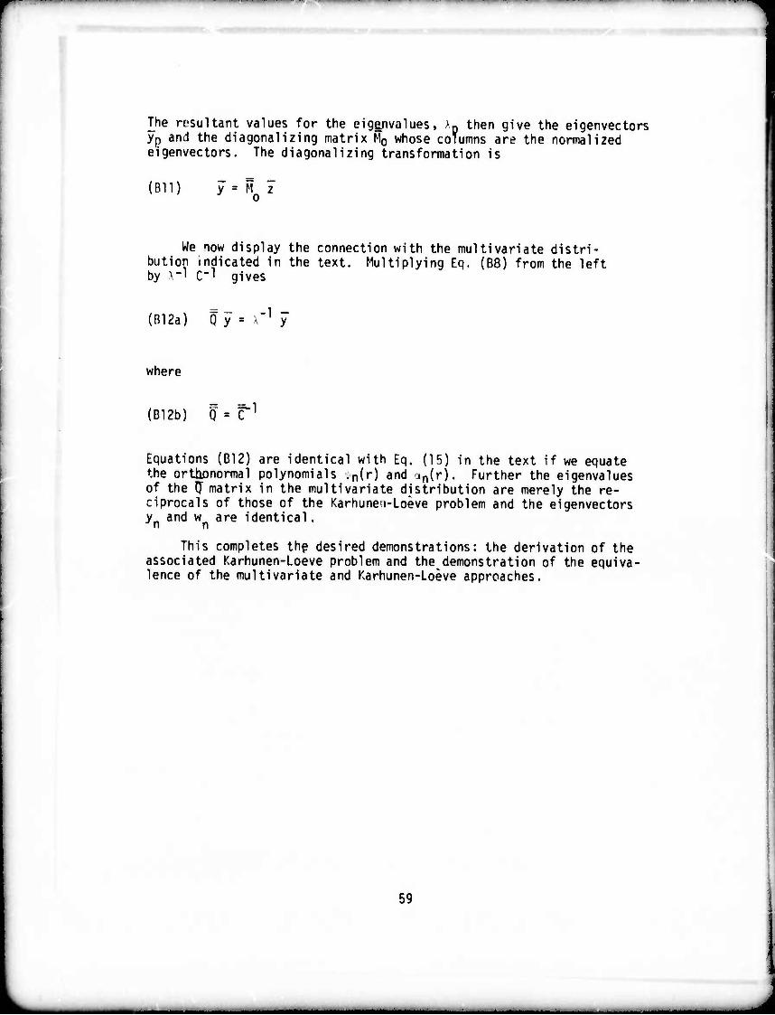
The resultant values for the eiganvalues, >p then give the eigenvectors yp and the diagonalizing matrix M0 whose coTumns are the normalized eigenvectors. The diagonalizing transformation is
(Bll) y = M z
We now display the connection with the multivariate distri- bution indicated in the text. Multiplying Eq. (B8) from the left by \-l C-l gives
(R12a) Q y ■ \m} y
where
(B12b) Q = C 1
Equations {B12) are identical with Eq. (15) in the text if we equate the ortiionormal polynomials .n(r) and in(r). Further the eigenvalues of the ^matrix in the multivariate distribution are merely the re- ciprocals of those of the Karhuneu-Loeve problem and the eigenvectors y and w,, are identical
This completes the desired demonstrations: the derivation of the associated Karhunen-Loeve problem and the demonstration of the equiva- lence of the multivariate and Karhunen-Loeve approaches.
59

APPENDIX C
Ue now derive expressions for the functions Un(K n,L n) and V(Mx0 Nxn) which were introduced in the main test ^qs.^Jin the niai n text.
for thl^cV0'? 0(f 9?nerali^' * «»^PlV only the development
tor the phase. To begin, assume that the orthonormal functions are polynomials in x a- j y so that in general
(C-l) (x.y) - i g xPy\
Inborn ""^ aPertUre the fUnCti0n Vn(Mxo'Nxo) ™ * «ritten
(C-2)
where
(C-3)
Vn(Mx0'
Nx0) " I %DJDW L(N) npq ps • 'q'
Iq(N) f 0
i-x0/2 dx x^
I > ..nc-[^ - (N-33)
in thl^ ^^^U^-o.L'o) «" Eq. (29a) can also be written in the more detailed form.
(C-4)
where
(C-5)
U(K>o'L'o) = ^ 'npcVS,)^)
N
0 M=l 1 0 1 0'
thr.n11nhri|t^ ^J^Tl«11 ^^^ in *<**' W the functions U0(K ,L ) through UgClCic ,U ) have the following form: 0 o,L o;
60

(C6a) VKk0.U0) ■ T0(K.o)To(L.o)
(C6b) U,(l*0.Kk0) ■ i!/rT0(fe0)T,(U )
(C6c) U2(l*0.Lk0) ■ -2jT,(K.0)T0(U0
(»a, UjdCk^lk,,) = 6 | [T0(K.o)T2(L.0) * T^K. o)To(L.o)
■I To(K-o'To(L.0):
(C«.l U4(Kk0.lk0) ■ 6:| [T0(K.0)T2(k.0) - T2(K.o)To(L.0)]
tC«f) U5(kk0.Lk0) ■ -12 1,(^)1,(1«,,)
(C69) ll6(l(k0,Lk0) ■ 127» [T2(IC«0)T,(2«0) - 1 T„(K. ^7,(1.^]
(C6h) U7(l(k0.Lk0) - -V.nn^0)J2{l.o) -jyT^fe,,) T0(L,0)]
1C61) U8(Kk0,lk0) - 2Q/7 [r0(r0)T3(L.0) - ^^(K.^T^L^)]
(«j) U, (Kko.Lk0) ■ -20.7 [:,(.:■ „IVS' " k WWJ
61
?— ■ "••.••
■
APPENDIX D
This appendix contains a listing of the sixty four eigenvalues of a solution for the Karhunen-Loeve integral equation assuming an eight by eight grid for the aperture plane. The correlation function corresponded to the phase function calculated in Appendix A.
EIGENVALUES
.9999E 0 ■ ■(0,0) .1875E -5 "(0,1)
.9220E -7 • ■(2.0) .4423E -7 -(2,1)
.1802E -7 .1590E -7
.8486E -8 .8486E -8
.4575E -8 .4162E -8
.3201E -8 .3015E -8
.2281E -P .2254E -8
.2005E -8 .1958E -8
.1586E -8 .1563E -8
.1461E -8 .1461E -8
.1249E -8 .1232E -8
.1071E -8 .1065E -8
.9478E -9 .8773E -9
.1875E -5 -(1,0)
.4423E -7 -(1,2)
.1323E -7
.6235E -8
.4044E -8
.3014E -8
.2109E -8
.1742E -8
.1563E -8
.1344E -8
.1203E -8
.1065E -8
.8772E -9
.1599E -6 -(1,1)
.2537E -7 -(0,3)
.8994E -8
.6234E -8
.4043E -8
.2565E -8
.2034E -8
.1712E -8
.1479E -8
.1343E -8
.1199E -8
.9599E -9
.8269E -9
.1347E -6 (0,2)
.2537E -7 (3,0)
.8636E -8
.4873E -8
.3321E -8
.2565E -8
.2006E -8
.1586E -8
.1474E -8
.1264E -8
.1072E -8
.9580E -9
62


MISSION of
Rome Air Development Center
MDC is the principal AFSC organization charged with planning and executing the USAF exploratory and advanced development programs for information sciences, intelli- gence, command, control and communications technology, products and sei vices oriented to tho needs of the USÄF. Primary RADC mission areas are communications, electro- magnetic guidance and control, surveillance of ground and aerospace objects, intelligence data collection and handling, information system technology, and electronic reliability, maintainability and compatibility. RADC has mission responsibility as assigned by AFSC for de- monstration and acquisition of selected subsystems arid systems in the intelligence, mapping, charting, command, control ana communications areas.
i