ACTIVE VIBRATION CONTROL OF A FLEXIBLE BASE MANIPULATOR

A Dissertation Presented to

The Academic Faculty

By

Lynnane E. George

In Partial Fulfillment Of the Requirements for the Degree

Doctor of Philosophy in Mechanical Engineering

Georgia Institute of Technology July 2002

Copyright 2002 by Lynnane Ellis George

ii

Active Vibration Control of a Flexible Base Manipulator

Approved: ____________________________________ Dr. Wayne Book, Chairman

___________________________________________

Dr. Anthony Calise

__________________________________ Dr. Al Ferri

____________________________________Dr. William Singhose

____________________________________ Dr. David Taylor

Date Approved: ______________________

iii

DEDICATION

To my grandparents:

Iva Frances Adamson

Dolzey Paul Borel

iv

ACKNOWLEDGEMENTS

Intellectual and Technical Support

First, I would like to thank my advisor, Dr. Wayne Book, for the advice and guidance

over the years working on this project. In addition, I would like to thank my committee

members for suggestions, advice, and guidance along the way. The Intelligent Machine

Dynamics Lab group also provided me many opportunities to present my work and get

feedback on various aspects of this project. In particular, I would like to thank my long-

term office mates, Davin Swanson, L.J. Tognetti, and Saghir Munir, for the many hours

of discussion, advice, and assistance.

Personal Support

My husband, Tom George, has always been there and supportive throughout our years of

marriage. In addition, I would like to thank my parents Herschel and Joyce Ellis, for

their support in many ways over the years.

Financial Support

Partial funding for this work was provided by the Air Force Institute of Technology U.S.

Air Force Academy Faculty Preparation Program and the HUSCO/Ramirez Endowed

Chair for Fluid Power and Motion Control

v

Disclaimer

The views expressed in this document are those of the author and do not reflect the

official policy or position of the United States Air Force, Department of Defense, or U.S.

Government

vi

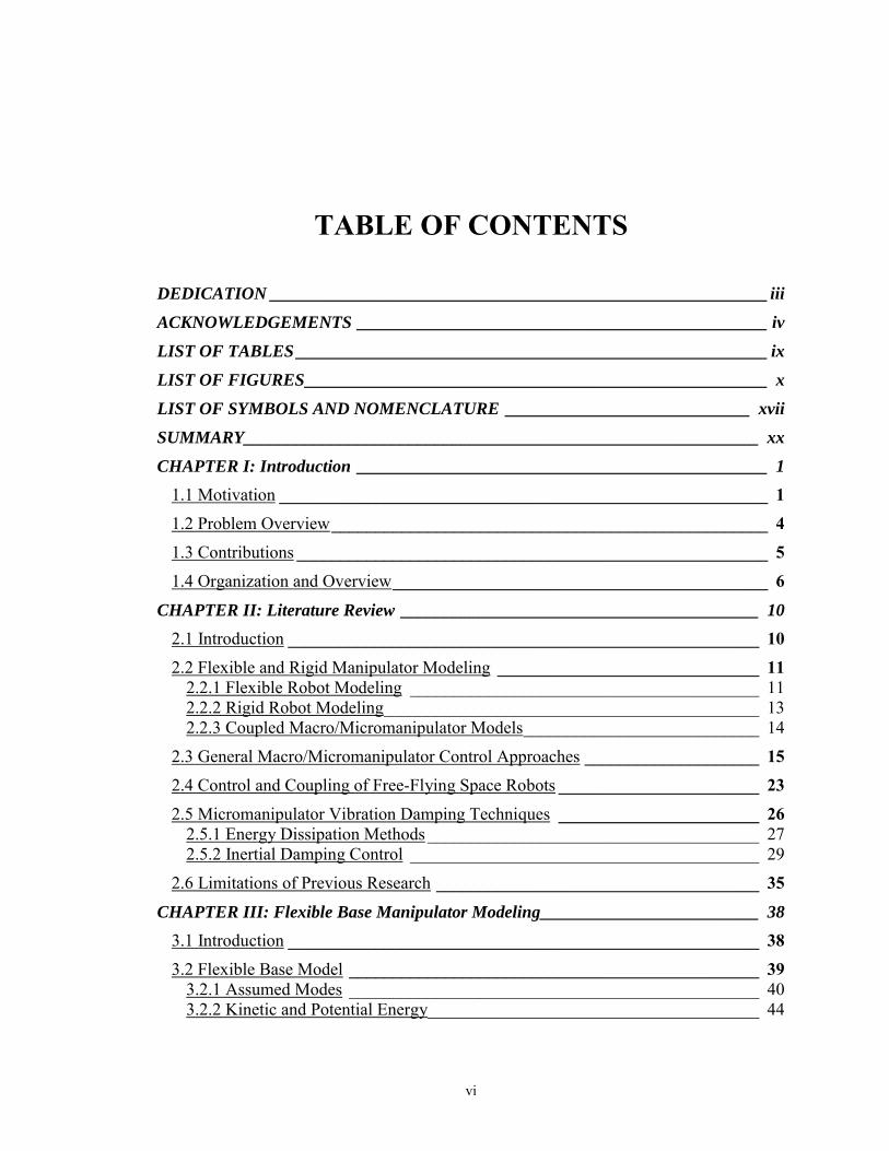
TABLE OF CONTENTS

DEDICATION _________________________________________________________ iii ACKNOWLEDGEMENTS _______________________________________________ iv LIST OF TABLES ______________________________________________________ ix LIST OF FIGURES_____________________________________________________ x LIST OF SYMBOLS AND NOMENCLATURE ____________________________ xvii SUMMARY___________________________________________________________ xx CHAPTER I: Introduction _______________________________________________ 1

1.1 Motivation ________________________________________________________ 1 1.2 Problem Overview__________________________________________________ 4 1.3 Contributions ______________________________________________________ 5 1.4 Organization and Overview___________________________________________ 6

CHAPTER II: Literature Review _________________________________________ 10 2.1 Introduction ______________________________________________________ 10 2.2 Flexible and Rigid Manipulator Modeling ______________________________ 11

2.2.1 Flexible Robot Modeling ________________________________________ 11 2.2.2 Rigid Robot Modeling___________________________________________ 13 2.2.3 Coupled Macro/Micromanipulator Models___________________________ 14

2.3 General Macro/Micromanipulator Control Approaches ____________________ 15 2.4 Control and Coupling of Free-Flying Space Robots _______________________ 23 2.5 Micromanipulator Vibration Damping Techniques _______________________ 26

2.5.1 Energy Dissipation Methods ______________________________________ 27 2.5.2 Inertial Damping Control ________________________________________ 29

2.6 Limitations of Previous Research _____________________________________ 35

CHAPTER III: Flexible Base Manipulator Modeling_________________________ 38 3.1 Introduction ______________________________________________________ 38 3.2 Flexible Base Model _______________________________________________ 39

3.2.1 Assumed Modes _______________________________________________ 40 3.2.2 Kinetic and Potential Energy______________________________________ 44

vii

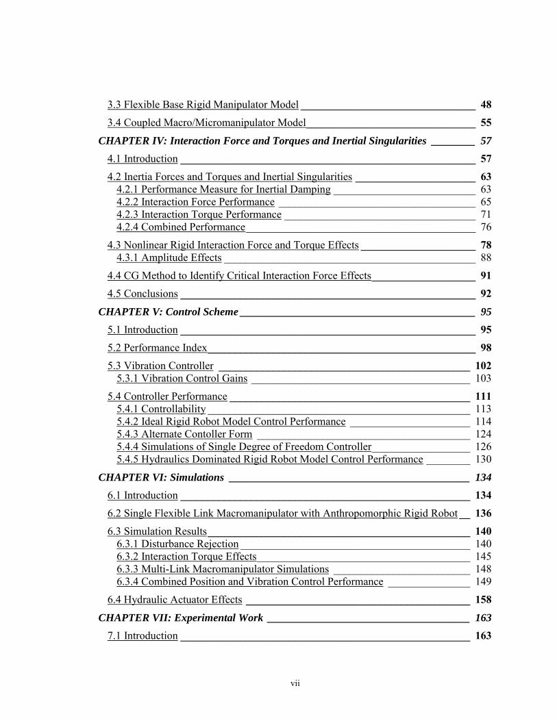
3.3 Flexible Base Rigid Manipulator Model ________________________________ 48 3.4 Coupled Macro/Micromanipulator Model_______________________________ 55

CHAPTER IV: Interaction Force and Torques and Inertial Singularities ________ 57 4.1 Introduction ______________________________________________________ 57 4.2 Inertia Forces and Torques and Inertial Singularities ______________________ 63

4.2.1 Performance Measure for Inertial Damping __________________________ 63 4.2.2 Interaction Force Performance ____________________________________ 65 4.2.3 Interaction Torque Performance ___________________________________ 71 4.2.4 Combined Performance__________________________________________ 76

4.3 Nonlinear Rigid Interaction Force and Torque Effects _____________________ 78 4.3.1 Amplitude Effects ______________________________________________ 88

4.4 CG Method to Identify Critical Interaction Force Effects___________________ 91 4.5 Conclusions ______________________________________________________ 92

CHAPTER V: Control Scheme ___________________________________________ 95 5.1 Introduction ______________________________________________________ 95 5.2 Performance Index_________________________________________________ 98 5.3 Vibration Controller ______________________________________________ 102

5.3.1 Vibration Control Gains ________________________________________ 103

5.4 Controller Performance ____________________________________________ 111 5.4.1 Controllability ________________________________________________ 113 5.4.2 Ideal Rigid Robot Model Control Performance ______________________ 114 5.4.3 Alternate Contoller Form _______________________________________ 124 5.4.4 Simulations of Single Degree of Freedom Controller__________________ 126 5.4.5 Hydraulics Dominated Rigid Robot Model Control Performance ________ 130

CHAPTER VI: Simulations ____________________________________________ 134 6.1 Introduction _____________________________________________________ 134 6.2 Single Flexible Link Macromanipulator with Anthropomorphic Rigid Robot __ 136 6.3 Simulation Results________________________________________________ 140

6.3.1 Disturbance Rejection __________________________________________ 140 6.3.2 Interaction Torque Effects_______________________________________ 145 6.3.3 Multi-Link Macromanipulator Simulations _________________________ 148 6.3.4 Combined Position and Vibration Control Performance _______________ 149

6.4 Hydraulic Actuator Effects _________________________________________ 158

CHAPTER VII: Experimental Work _____________________________________ 163 7.1 Introduction _____________________________________________________ 163

viii

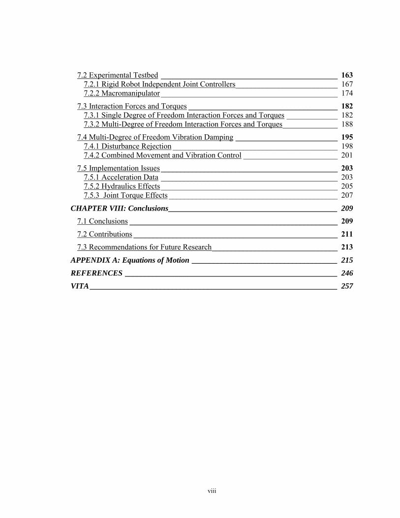
7.2 Experimental Testbed _____________________________________________ 163 7.2.1 Rigid Robot Independent Joint Controllers__________________________ 167 7.2.2 Macromanipulator _____________________________________________ 174

7.3 Interaction Forces and Torques ______________________________________ 182 7.3.1 Single Degree of Freedom Interaction Forces and Torques _____________ 182 7.3.2 Multi-Degree of Freedom Interaction Forces and Torques______________ 188

7.4 Multi-Degree of Freedom Vibration Damping __________________________ 195 7.4.1 Disturbance Rejection __________________________________________ 198 7.4.2 Combined Movement and Vibration Control ________________________ 201

7.5 Implementation Issues _____________________________________________ 203 7.5.1 Acceleration Data _____________________________________________ 203 7.5.2 Hydraulics Effects_____________________________________________ 205 7.5.3 Joint Torque Effects ___________________________________________ 207

CHAPTER VIII: Conclusions___________________________________________ 209 7.1 Conclusions _____________________________________________________ 209 7.2 Contributions ____________________________________________________ 211 7.3 Recommendations for Future Research________________________________ 213

APPENDIX A: Equations of Motion _____________________________________ 215 REFERENCES ______________________________________________________ 246 VITA _______________________________________________________________ 257

ix

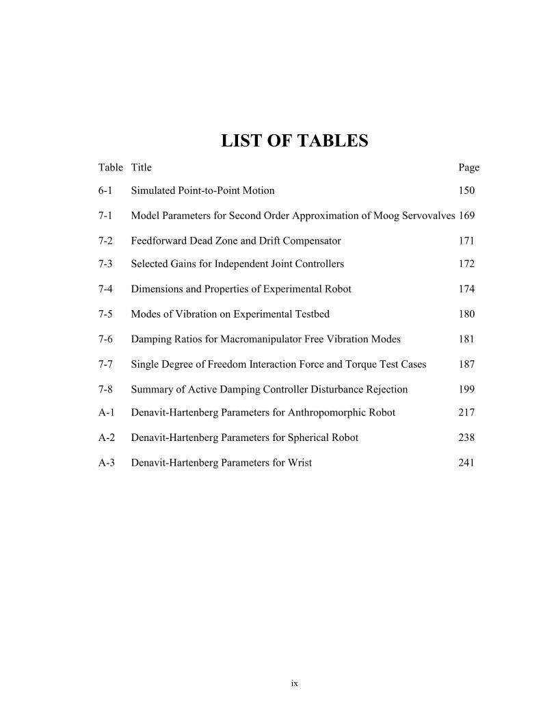
LIST OF TABLES

Table Title Page 6-1 Simulated Point-to-Point Motion 150 7-1 Model Parameters for Second Order Approximation of Moog Servovalves 169 7-2 Feedforward Dead Zone and Drift Compensator 171 7-3 Selected Gains for Independent Joint Controllers 172 7-4 Dimensions and Properties of Experimental Robot 174 7-5 Modes of Vibration on Experimental Testbed 180 7-6 Damping Ratios for Macromanipulator Free Vibration Modes 181 7-7 Single Degree of Freedom Interaction Force and Torque Test Cases 187 7-8 Summary of Active Damping Controller Disturbance Rejection 199

A-1 Denavit-Hartenberg Parameters for Anthropomorphic Robot 217 A-2 Denavit-Hartenberg Parameters for Spherical Robot 238 A-3 Denavit-Hartenberg Parameters for Wrist 241

x

LIST OF FIGURES

Figure Page 1-1 Macro/Micro Manipulator 2 1-2 Flexible Base Manipulator 2 1-3 Overview of Control Scheme 8 3-1 Flexible Link Model Notation 41 3-2 Flexible Base Rigid Robot 49 3-3 Flexible Base Single Link Rigid Robot 50 3-4 Notation Used for Recursive Newton-Euler Algorithm 53 4-1 3 DOF Anthropomorphic Robot 60 4-2 3 DOF Spherical Robot 61 4-3 3 DOF Wrist Robot 61 4-4 6 DOF Anthropomorphic Robot with Wrist 62 4-5 Force Performance � 3 DOF Anthropomorphic Robot 66 4-6 Force Performance � 3 DOF Spherical Robot 67 4-7 Force Performance � 3 DOF Wrist Robot 68 4-8 Torque Performance � 2 DOF Anthropomorphic Robot 73 4-9 Torque Performance � 3 DOF Spherical Robot 74 4-10 Torque Performance � 3 DOF Wrist Robot 75 4-11 Combined Force and Torque Performance � 3 DOF

Anthropomorphic Robot 76

xi

4-12 Combined Force and Torque Performance � 3 DOF Spherical Robot 77

4-13 Anthropomorphic Robot Coriolis Forces 80 4-14 Anthropomorphic Robot Centrifugal Forces 81 4-15 Anthropomorphic Robot Inertia Forces 81 4-16 Spherical Robot Coriolis Torques 83 4-17 Spherical Robot Centrifugal Torques 84 4-18 Spherical Robot Inertia Torques 84 4-19 Anthropomorophic Interaction Forces, Large Inertia Effects 85 4-20 Anthropomorphic Interaction Forces, Near Singularity Case 2 86 4-21 Anthropomorphic Interaction Forces, Large Centrifugal Effects 87 4-22 Anthropomorphic Configuration with Large Nonlinear Forces 88 4-23 Effect of Reducing Joint Amplitudes on Nonlinear Effects 90 4-24 Alternate Inverse Kinematic Configurations for

Anthropomorphic Robot 93 5-1 Combined Position and Base Vibration Control Scheme 95 5-2 Linearized Single Degree of Freedom Control Scheme 112 5-3 Pole-Zero Map of Closed Loop System 116 5-4 Root Locus for Increasing Vibration Control Feedback Gains 118 5-5 Root Locus for Increasing Position Control Feedback Gains 118 5-6 Root Locus with Poor Selection of Vibration and Rigid Position Controllers 121 5-7 Root Locus with Better Selection of Vibration and Rigid Position

Controllers 121

xii

5-8 Effect of Choosing Vibration Control Zero too Large 122 5-9 Effect of Choosing Vibration Control Zero too Small 122 5-10 Root Locus for Velocity Feedback, Ideal Model 123 5-11 Alternate Form of Vibration Controller 124 5-12 Pole-Zero Map of Alternate Controller 125 5-13 Single Degree of Freedom Matlab Simulation 126 5-14 Single Degree of Freedom Flexible Base Manipulator 126 5-15 Simulated Base Motion Due to an Applied Disturbance 127 5-16 Simulated Joint Motion with Inertial Damping Due to an Applied Disturbance 128 5-17 Simulated Commanded Joint Motion 128 5-18 Simulated Base Vibration Due to Commanded Joint Motion 129 5-19 Simulated Inertial Damping Performance with Velocity Feedback 129 5-20 Actuator Dominated Linearized Rigid Robot Model 130 5-21 Form of Vibration Controller for Hydraulics Dominated Robot 131 5-22 Root Locus for Increasing Vibration Control Gains, Hydraulics

Model 132

5-23 Root Locus for Increasing Position Control Gains, Hydraulics Model 133

6-1 Matlab Simulation 137 6-2 Anthropomorphic Robot Configuration [45°,20°,-70°] 141 6-3 Simulated Base Vibration Due to an Applied Disturbance 141 6-4 Simulated Joint Motion Due to an Applied Disturbance 142 6-5 Simulated Total End Point Position Due to an Applied Disturbance 142

xiii

6-6 Simulated Base Vibration Due to an Applied Disturbance, Large Vibration Control Gains 143

6-7 Simulated Joint Motion Due to an Applied Disturbance, Large Vibration Control Gains 144

6-8 Simulated Base Vibration with Robot in a Region with Large Nonlinear Effects 145 6-9 Simulated Joint Motion with Robot in a Region with Large Nonlinear Effects 146 6-10 Simulated Base Vibration with Interaction Forces and Torques Modeled, Configuration [45°,45°,-70°] 147 6-11 Simulated Base Vibration With Interaction Forces and Torques

Modeled, Configuration [-90°,45°,-70°] 148

6-12 Simulated Base Vibration x Due to Point-to-Point Motion 151 6-13 Simulated Base Vibration y Due to Point-to-Point Motion 152 6-14 Simulated Base Vibration z Due to Point-to-Point Motion 152 6-15 Simulated Joint 1 Motion During Point-to-Point Motion 153 6-16 Simulated Joint Motion during Point-to-Point Motion 153 6-17 Simulated Total End Point Position x During Point-to-Point

Motion 154 6-18 Simulated Total End Point Position y During Point-to-Point

Motion 155 6-19 Base Vibration x with Reduced Gains for Damping Controller 157 6-20 Root Locus for Single Degree of Freedom Ideal Linearized Model 157 6-21 Hydraulics Dominated Single Degree of Freedom Model 158 6-22 Baseline Performance with Joint 2 Hydraulics Model 160 6-23 Phasing of Joint Actuation and Base Vibration, Hydraulics Model 160

xiv

6-24 Effect of Increasing Phase Lag on Hydraulics Model Vibration Performance 161

6-25 Phasing of Joint Actuation and Base Vibration, Hydraulics Modeled with Higher Order Dynamics 162

7-1 Laboratory Setup 166 7-2 Experimental Rigid Robot 168 7-3 Independent Joint Controller 168 7-4 Joint 1 Response to D/A Output of �100 170 7-5 Dead Zone Phenomenon in Hydraulic Servovalve 172 7-6 Root Locus Design for Independent Joint Controllers 173 7-7 Macromanipulator Base Mounting 175 7-8 Overall Macro/Micromanipulator Testbed 176 7-9 Free Vibration x Due to an Applied Disturbance x 177 7-10 Frequency Content of x Vibration Due to an Applied

Disturbance x 178

7-11 Position x Due to an Applied Disturbance x 179 7-12 Frequency Content of x Position Data Due to an Applied Disturbance x 179 7-13 Position y Due to an Applied Disturbance x 181 7-14 Braced Micromanipulator 184 7-15 Predicted and Measured Interaction Forces at the Base of the

Micromanipulator Due to Joint 1 Harmonic Motion 185

7-16 Predicted and Measured Interaction Torques at the Base of the Micromanipulator Due to Joint 1 Harmonic Motion 186

xv

7-17 Predicted and Measured Interaction Forces Due to Joints 1,2, and 3 Actuating Simultaneously 188 7-18 Frequency Content of Force y Data Due to Joints 1,2,and 3

Actuating Simultaneously 189 7-19 Anthropomorphic Robot Configuration [0°, 87°, 56°] 190 7-20 Interaction Forces Due to Joints 1 and 2 Actuating Near an Inertial

Singularity 190

7-21 Frequency Content of Force Data due to Joints 1 and 2 Actuating Near an Inertial Singularity 191

7-22 Anthropomorphic Robot Configuration [0°,38°,0°] 192 7-23 Interaction Forces with Large Centrifugal Effects Due to Joints 1, 2, and 3 Actuating Simultaneously 192 7-24 Frequency Content of Force x data with Large Centrifugal 193

Effects

7-25 Interaction Torques due to Joints 1, 2, and 3 in Configuration (0°,38°,0°) 193 7-26 Frequency Content of Interaction Torque Data Due to

Joints 1, 2, and 3 194 7-27 Block Diagram of Multi-Degree of Freedom Vibration Damping 197 7-28 Vibration Control Due to an Applied Disturbance 200 7-29 Joint Response Due to an Applied Disturbance 200 7-30 Base Vibration Due to Commanded Movement 202

7-31 Joint Motion during Commanded Point-to-Point Movement with

Vibration Control 202

7-32 Base Vibration Due to Commanded Movement in Region with Predicted Poor Inertial Damping Performance 203

7-33 Low Frequency Tracking of Joint 2 206

xvi

7-34 High Frequency Tracking of Joint 2 206 7-35 Testbed Configuration with Poor Inertial Damping Performance 208

xvii

LIST OF SYMBOLS AND NOMENCLATURE

ai,di: Length of link i of the rigid robot

Bf (θθθθ): Rigid manipulator interaction force inertia matrix

Bτ0(θθθθ): Rigid manipulator interaction torque inertia matrix

f

τ0

B ( )B( ) : Total rigid robot interaction inertia matrix=

B ( )

θθ

θ

Bτ(θθθθ): Rigid manipulator inertia matrix

C(q): Macromanipulator translational damping matrix

Cr(q): Macromanipulator rotational damping matrix

CG: Center of gravity

DOF: Degree of freedom

FIF : Interaction forces between the micro and macromanipulator=[Fx Fy Fz]T

Ijkk: Moment of inertia of link j of the rigid robot about the kth axis

ID: Inverse dynamics function

J(q): Macromanipulator mass moment of inertia matrix

Ki: Vibration control feedback gain for ith macromanipulator DOF

K(q): Macromanipulator translational stiffness matrix

Kr(q): Macromanipulator rotational stiffness matrix

mi: Mass of the ith link of the rigid robot

M(q): Macromanipulator mass matrix

xviii

NCf (θθθθ): Rigid robot centrifugal interaction force matrix

NCτ0(θθθθ): Rigid robot centrifugal interaction torque matrix

Nf (θθθθ): Total rigid robot nonlinear interaction force matrix (centrifugal and coriolis)

NRf (θθθθ): Rigid robot coriolis interaction force matrix

NRτ0(θθθθ): Rigid robot coriolis interaction torque matrix

Nτ0(θθθθ): Total rigid robot nonlinear interaction torque matrix (centrifugal and coriolis)

PD: Proportional and derivative controller

PID: Proportional, derivative, and integral controller

PI: Performance Index q: Flexible manipulator generalized coordinates

q% : Flexible manipulator generalized coordinates linearized about an operating point

Q: Generalized force applied by the micromanipulator to the macromanipulator

rcg: Position vector to the overall CG of the robot

Rii-1: Rotation matrix of frame i with respect to frame i-1

T: Kinetic Energy

V: Potential Energy

Wf: Flexible robot weighting matrix

Wr: Rigid robot weighting matrix

xf: Flexible base translational motion =[x y z]T

Xi: Amplitude of vibration of the ith mode of the flexible base

xd: Desired rigid robot end point position

δ: Disturbance force

xix

ζ: Damping ratio

θθθθ or θθθθa: Actual rigid manipulator joint variables=[θ1 θ2 θ3 �θn]T

θ% : Rigid manipulator joint variables linearized about an operating point

θθθθd: Desired rigid manipulator joint variables=[θ1d θ2d θ3d �θnd]T

θθθθf: Flexible base rotational motion=[θx θy θz]T

θi: Rigid robot ith joint angle

ττττ : Rigid robot joint actuation torques=[τ1 τ2 τ3 �τn]T

ττττIF : Interaction torques between the micro and macromanipulator=[τx τy τz]T

ωi: Natural frequency of the ith mode of the flexible base

xx

SUMMARY

A rigid (micro) robot mounted serially to the tip of a long, flexible (macro) robot

is often used to increase reach capability, but flexibility in the macromanipulator can

make it susceptible to vibration. A rigid manipulator attached to a flexible but unactuated

base was used to study a scheme to achieve micromanipulator positioning combined with

vibration damping of the base. Inertial interaction forces and torques acting at the base of

the rigid robot were studied to determine how to use them to damp the base vibration.

The ability of the rigid robot to create inertial interactions varies throughout the

workspace. There are also �inertial singularity� configurations where the robot loses its

ability to create interactions in one or more degrees of freedom. A performance index

was developed to quantify this variation in performance and can be used to ensure the

robot operates in joint space configurations favorable for inertial damping. When the

performance index is used along with appropriate vibration control feedback gains, the

inertia effects, or those directly due to accelerating the rigid robot links, have the greatest

influence on the interactions. By commanding the link accelerations out of phase with

the base vibration, energy will be removed from the system. This signal is then added to

the rigid robot position control signal. Simulated and measured interaction forces and

torques generated at the base of a rigid robot are compared to verify conclusions drawn

about the controllable interactions. In addition, simulated and experimental results

demonstrate the combined position control and vibration damping ability of the scheme.

1

CHAPTER I

INTRODUCTION

1.1 Motivation

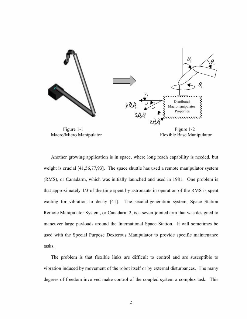
The objective of this research was to develop a combined position and enhanced

vibration control scheme for a rigid manipulator attached to a flexible base. The

configuration is similar to a macro/micromanipulator (Figure 1-1), which has links that

are long and lightweight with a rigid robot attached serially to the end. Macro/micro

manipulators are desirable for certain uses, because the macromanipulator can provide

long reach capability by moving the robot to the general area of interest where it can then

be used for fine-tuned positioning. These are often used to perform tasks that humans

may be incapable of doing or that are dangerous for humans.

One application is in the nuclear industry where macro/micromanipulators are used to

remove nuclear waste from underground storage tanks [25]. In the application described

in the reference, a 39 foot, seven degree of freedom long-reach manipulator was used

with a rigid end effector to clean seven storage tanks at Oak Ridge National Laboratory

from 1996-2000. Two end effectors were used: one type measured the radiation field,

while the other scarified the tank walls.

2

Figure 1-1 Figure 1-2 Macro/Micro Manipulator Flexible Base Manipulator Another growing application is in space, where long reach capability is needed, but

weight is crucial [41,56,77,93]. The space shuttle has used a remote manipulator system

(RMS), or Canadarm, which was initially launched and used in 1981. One problem is

that approximately 1/3 of the time spent by astronauts in operation of the RMS is spent

waiting for vibration to decay [41]. The second-generation system, Space Station

Remote Manipulator System, or Canadarm 2, is a seven-jointed arm that was designed to

maneuver large payloads around the International Space Station. It will sometimes be

used with the Special Purpose Dexterous Manipulator to provide specific maintenance

tasks.

The problem is that flexible links are difficult to control and are susceptible to

vibration induced by movement of the robot itself or by external disturbances. The many

degrees of freedom involved make control of the coupled system a complex task. This

Distributed Macromanipulator

Properties , ,y yyθ θ&& &&&

, ,x xxθ θ&& &&&, ,z zzθ θ&& &&&

1θ

2θ3θ

3

research considers the base of the rigid robot to be flexible, where the base motion is

similar to that due to vibration at the tip of a flexible macromanipulator with locked joints

(Figure 1-2). It is assumed for this work the joints of the macromanipulator are not

actuating so the only vibration in the system is due to externally applied disturbances or

motion of the rigid manipulator.

Many researchers have tackled the problem of developing control schemes to

eliminate unwanted vibration in flexible manipulators. One area involves determining

trajectories that will avoid or minimize inducing vibration; however, these schemes are

not useful for controlling vibration once it occurs. The macromanipulator actuators are

not a good option for vibration damping due to bandwidth limitations and non-collocation

of the actuators and end point vibration. This creates a non-minimum phase problem due

to time delays, further exacerbated by flexibility in the link(s). In addition, since only

gross positioning capability is really needed for the macromanipulator, it is an

unnecessary increase in cost and system complexity to use its actuators for vibration

control in addition to their already difficult task.

The use of the rigid manipulator to damp vibration in the macromanipulator has

proven to be a promising area. The micromanipulator produces inertial forces and

torques that act as disturbances to the macromanipulator under decoupled control. Under

coupled control, these inertial effects can be used as damping forces and torques and

applied directly to the tip of the macromanipulator. This also makes the system

minimum phase, further reducing the complexity of the control task. In addition, it is

much easier to provide high bandwidth actuators for a small robot arm than for a large

4

one, so its actuators can respond more quickly and efficiently to provide large inertial

forces and torques. Previous methods of damping vibration in this manner include

energy dissipation methods and inertial damping methods. The goal here is to command

the rigid robot to act as an active vibration damper, damping the motion of the

macromanipulator at the natural frequencies of the system. These along with other

methods of controlling macro/micromanipulators are discussed in more detail in Chapter

2.

1.2 Problem Overview

In this work, the rigid robot control scheme must perform the dual task of damping

unwanted base vibration (macromanipulator vibration) while providing position control

of the rigid robot. On the one hand, if the motion of the micromanipulator or combined

system is completely prescribed by the task, this method is not useful. However, under

circumstances where the task will allow small movements of the rigid robot to damp the

vibration, this technique can be very effective. After all, if the system is vibrating

uncontrollably the system performance is impacted. The controlled interactions are

collocated with the vibration at the tip of the macromanipulator, and the rigid robot can

respond quickly to create the inertial damping forces and torques. The goal here is to

reduce the vibration as quickly and efficiently as possible so the system can continue with

its task. This method requires no hardware modifications other than some type of

measurement of the vibration.

5

Most of the literature addresses macro/micromanipulator position control or vibration

control alone, but few researchers address both. The authors that have addressed both

assume limited base flexibility, thereby limiting the applicability of the work. In

addition, simulations and hardware demonstrations have been limited mostly to planar

translational vibration. Finally, operation throughout the workspace has not been

addressed, in particular at locations where coupling effects between the macro and

micromanipulator are unsuited to vibration damping.

The control scheme described in this dissertation was tested in simulations and

experiments in two main scenarios. The first was with the robot operating at a desired

joint space configuration and tested its ability to damp vibration induced by an applied

disturbance. The second scenario was for point-to-point motion where the rigid robot is

moving from an initial to a final joint space configuration in a given time period. Both of

these allow flexibility in choosing between alternate inverse kinematic joint space

configurations. If the joint space configuration of the rigid robot is a prescribed part of

the control scheme, another method of damping may be required.

1.3 Contributions

The contributions of this thesis are:

1. Extension of the macro/micromanipulator control problem to multiple degrees of

freedom by considering the analogous problem of a rigid manipulator mounted on a

flexible base.

6

2. Investigation of inertial singularities and variation in inertial damping performance

throughout the workspace.

3. Development of a control scheme that provides active base vibration damping in

parallel with rigid robot position control and establishment of appropriate vibration

control gain limits.

4. Verification of the above via simulation.

5. Experimental work including verification of the accuracy of the interaction force

and torque predictions and demonstration of the effectiveness of the control scheme on a

realistic multi-degree of freedom testbed.

1.4 Organization and Overview

This dissertation is organized in the following manner:

Chapter 1 discusses the motivation of the research, contributions of the work, and

outlines the dissertation.

Chapter 2 reviews the current state of literature on the subject of

macro/micromanipulator control and limitations of previous research.

Chapter 3 describes modeling of the flexible base manipulator. A Lagrangian

approach with a finite number of assumed modes was used to represent the flexible

manipulator, while a recursive Newton-Euler formulation was used to derive expressions

for the interaction forces and torques acting between the macro and micromanipulator.

The general form of these interactions is:

7

0 0 0 0 0

( ) ( , ) ( ) ( ) ( , , , )

( ) ( , ) ( ) ( ) ( , , , ) (1-1)IF f f i j f f fc

IF i j c

B N G C N

B N G C Nτ τ τ τ τ

= + + + +

= + + + +

F θ θ θ θ θ θ θ q q q θ θ

τ θ θ θ θ θ θ θ q q q θ θ

&& & & &&& &

&& & & &&& &

where θθθθ represents the rigid robot joint variables and q represents the flexible

manipulator generalized coordinates. The rigid robot configuration, θθθθ, joint velocities

and accelerations, and flexible base velocities and accelerations drive the interactions.

The goal was to study these interactions in order to determine how to use them in the

control scheme to damp the macromanipulator vibration.

Chapter 4 discusses in more detail the controllable interactions, or the first two terms

in each equation in 1-1. A performance measure is introduced which predicts the

effectiveness of the rigid robot in creating these interactions. The rigid inertia effects

(Bf(θθθθ) and Bτ0(θθθθ)) are particularly important for two reasons. First, the rigid robot must

have enough inertia to effectively apply interaction forces and torques to the

macromanipulator. The ratio of the rigid inertia to flexible inertia effects becomes an

important part of the performance index, discussed in Chapter 5. Second, there are joint

workspace configurations where these matrices become singular. These �inertial

singularities� represent physical limitations in that an inertia force or torque cannot be

created in one or more degrees of freedom. The variation in performance is driven by the

joint space configuration of the rigid robot, so the performance measure can be used to

choose joint space configurations better suited for inertial damping. The inertia effects

dominate the interactions in most non-singular configurations. However, the nonlinear

rigid effects may also become significant in certain cases and these are also discussed

here.

8

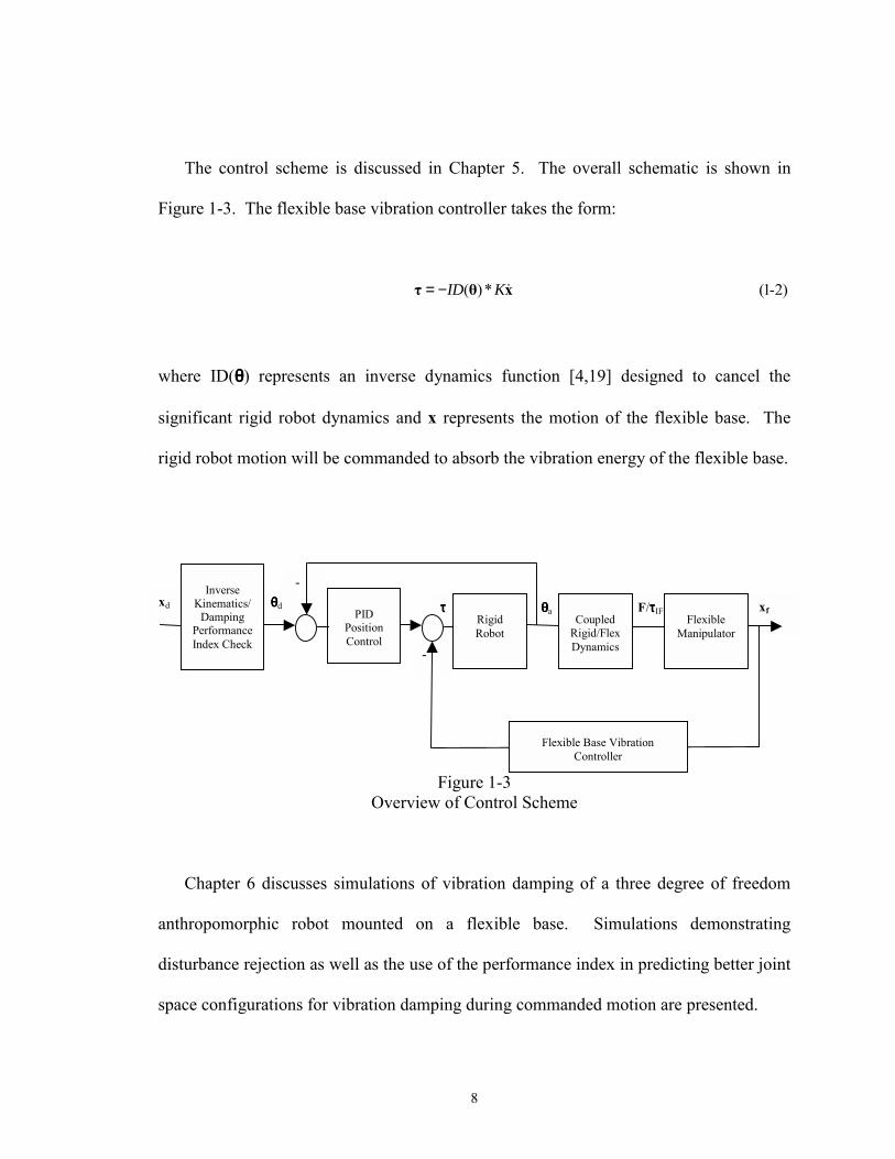
The control scheme is discussed in Chapter 5. The overall schematic is shown in

Figure 1-3. The flexible base vibration controller takes the form:

( )* (1-2)ID K= −τ θ x&

where ID(θθθθ) represents an inverse dynamics function [4,19] designed to cancel the

significant rigid robot dynamics and x represents the motion of the flexible base. The

rigid robot motion will be commanded to absorb the vibration energy of the flexible base.

Figure 1-3 Overview of Control Scheme

Chapter 6 discusses simulations of vibration damping of a three degree of freedom

anthropomorphic robot mounted on a flexible base. Simulations demonstrating

disturbance rejection as well as the use of the performance index in predicting better joint

space configurations for vibration damping during commanded motion are presented.

xf ττττ

-

-

θθθθd θθθθa

PID Position Control

F/ττττIF

Flexible Base Vibration Controller

xd

Inverse

Kinematics/ Damping

Performance Index Check

Rigid Robot

Coupled

Rigid/FlexDynamics

Flexible

Manipulator

9

Chapter 7 discusses the experimental testbed and presents results from two areas of

testing. First, predicted and measured interaction forces and torques generated at the base

of a rigid three degree of freedom anthropomorphic robot are presented, which verified

many of the results presented in Chapter 4. Second, the ability of the controller to damp

vibration on a multi-degree of freedom testbed was tested. The macromanipulator

consists of two flexible links in a fixed joint configuration. Three links of a six degree of

freedom micromanipulator were used for vibration damping. Some promising results are

presented demonstrating overall vibration energy from the system. However, several

implementation issues arose that limited the effectiveness of the scheme on the testbed.

These are discussed in more detail as well as proposed means of addressing these issues

for future work.

Chapter 8 summarizes the results and suggests area of further research. Finally,

Appendix A includes the equations for the interaction forces and torques for four typical

robot configurations.

10

CHAPTER II

LITERATURE REVIEW

2.1 Introduction

This chapter reviews the general topic of macro/micromanipulator control.

Macro/micromanipulators were introduced in the early 1980s as a means of improving

endpoint control of flexible manipulators, which were becoming more common for

applications where long reach capability was needed. Positioning errors due to flexibility

and other inaccuracies in the links of the macromanipulator are compensated for by the

micromanipulator.

First, literature on modeling flexible and rigid manipulators is reviewed. Since this in

itself is a very broad area, the research discussed here is specifically relevant to modeling

combined flexible/rigid systems. Next, general methods of controlling

macro/micromanipulators are discussed. The problem that becomes quickly apparent is

the large number of degrees of freedom involved and complexity of the resulting control

problem. The links of the macromanipulator are susceptible to vibration, so there are

additional degrees of freedom that need to be controlled as well as the rigid coordinates.

One option to reduce the complexity of the problem is to decouple control of the rigid

and flexible robots. In this case, the macromanipulator provides gross positioning while

the rigid robot provides the fine-tuned positioning. However, there are also problems

11

with this technique. The rigid robot produces inertial forces and torques which can act as

disturbances to the macromanipulator and worsen the vibration problem. In addition,

with larger and more flexible macromanipulators, vibration amplitudes can become too

large for the rigid robot to compensate for. Thus another area of research evolved which

focused on methods of commanding the micromanipulator to reduce vibration in the

macromanipulator. One way is to command the rigid robot using trajectories that will

reduce these disturbances. An alternate approach is to use the disturbances to damp the

vibration, which is the basis of the work described in this dissertation. The current state

of research in this area is reviewed as well as limitations of the work performed thus far.

In addition, there has been a great deal of related research in the area of space

robotics. This area has not been widely recognized as being related to the problem of

earth-based macro/micromanipulator control. However, the approach taken in this thesis,

where the rigid robot is considered attached to a flexible base, is very similar to space

robotics research that considers a rigid robot mounted to a floating base (spacecraft).

Some of the applicable space robotics research is also reviewed here.

2.2 Flexible and Rigid Manipulator Modeling 2.2.1 Flexible Robot Modeling

There are many methods available to model flexible link robots. Since the links are

distributed parameter systems, their motion is described by partial differential equations

instead of ordinary differential equations and hence modeling can become very

12

challenging. In addition to the nonlinear rigid dynamics commonly found in robotic

systems, flexible manipulators also exhibit elastic behavior.

Book [8] developed a recursive Lagrangian approach for modeling flexible link

robots. Describing the position of a point on a flexible link requires both rigid and elastic

coordinates, so he suggested the use of 4 x 4 transformation matrices for more compact

representation. By choosing a finite number of assumed modes to model the elastic

motion, the position of a point along each flexible link can be written in terms of the rigid

and flexible coordinates. Expressions for kinetic and potential energy of the system can

then be developed. The kinetic energy terms consist of translational and rotational

energy of each link. Potential energy terms consist of elastic bending, gravity, and

shearing deformation effects.

Several authors have considered the relative importance of the energy terms and

under what circumstances certain effects may be neglected [46,52,72,83]. Most authors

involved in modeling flexible manipulators assume Euler-Bernoulli bending theory

applies. When this is the case, rotational inertia terms may be assumed negligible, and

potential energy terms only need to include elastic bending and gravity effects [83]. The

resultant equations are integrated over the spatial variable and used with Lagrange�s

equations to derive the equations of motion. One advantage of this method is that the

energy terms can include as much or as little detail as needed. Modal damping may also

be added if desired. Regardless of the method used to derive them, the equations of

motion take the form:

13

= inertia matrix

nonlinear, coupling, and viscoelastic effects

stiffness matrix

gravitational effects

generalized forces

flexible coordinatesrigid j

( ) ( ) ( ) b b b b

b

b

b

b

f

r

M

C

K

G

M C K G

=

=

=

=

= =

+ + + =

Q

xq

θ

q q q,q q q Q&& &

oint coordinates

(2-1)

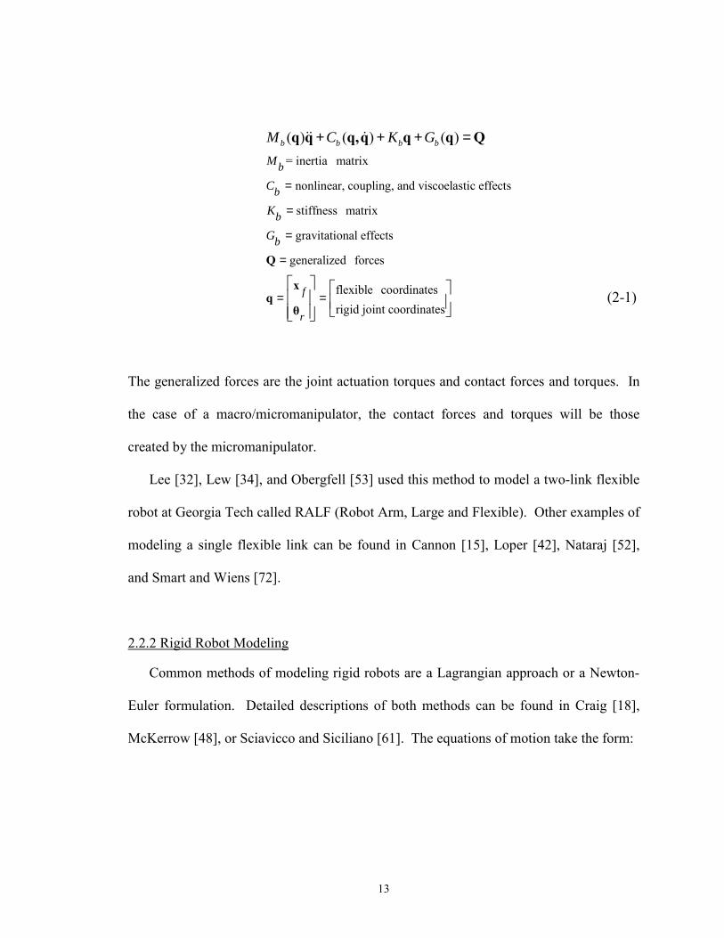
The generalized forces are the joint actuation torques and contact forces and torques. In

the case of a macro/micromanipulator, the contact forces and torques will be those

created by the micromanipulator.

Lee [32], Lew [34], and Obergfell [53] used this method to model a two-link flexible

robot at Georgia Tech called RALF (Robot Arm, Large and Flexible). Other examples of

modeling a single flexible link can be found in Cannon [15], Loper [42], Nataraj [52],

and Smart and Wiens [72].

2.2.2 Rigid Robot Modeling

Common methods of modeling rigid robots are a Lagrangian approach or a Newton-

Euler formulation. Detailed descriptions of both methods can be found in Craig [18],

McKerrow [48], or Sciavicco and Siciliano [61]. The equations of motion take the form:

14

( ) ( , ) ( )rigid joint coordinates

( ) symmetric, positive definite inertia matrix

N ( , ) centrifugal and coriolis effectsG ( )=gravitational effects

joint actuation torques

B N G

B

τ τ τ

τ

τ

τ

+ + ==

=

=

=

θ θ θ θ θ θ τθθ

θ θθ

τ

&& & &

&

(2-2)

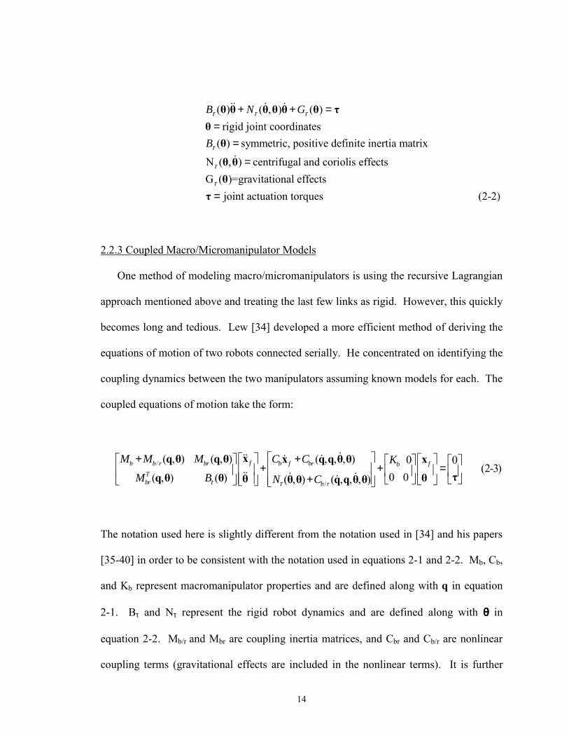
2.2.3 Coupled Macro/Micromanipulator Models

One method of modeling macro/micromanipulators is using the recursive Lagrangian

approach mentioned above and treating the last few links as rigid. However, this quickly

becomes long and tedious. Lew [34] developed a more efficient method of deriving the

equations of motion of two robots connected serially. He concentrated on identifying the

coupling dynamics between the two manipulators assuming known models for each. The

coupled equations of motion take the form:

/

/

( , ) ( , ) ( , , , ) 0 0 (2-3)

0 0 ( , ) ( ) ( , ) ( , , , )fb b r br b f br fb

Tbr b r

M M M C C KM B N Cτ τ

+ + + + = +

xq θ q θ x q q θ θ xτq θ θ θθ θ θ q q θ θ

&&& &&

&& & &&

The notation used here is slightly different from the notation used in [34] and his papers

[35-40] in order to be consistent with the notation used in equations 2-1 and 2-2. Mb, Cb,

and Kb represent macromanipulator properties and are defined along with q in equation

2-1. Bτ and Nτ represent the rigid robot dynamics and are defined along with θθθθ in

equation 2-2. Mb/r and Mbr are coupling inertia matrices, and Cbr and Cb/r are nonlinear

coupling terms (gravitational effects are included in the nonlinear terms). It is further

15

assumed the macromanipulator is not actuating so the only joint torques and rigid

coordinates that vary are those associated with the rigid robot. Most of the

macro/micromanipulator control literature uses this form of the coupled equations of

motion as a baseline model.

Sharf [63] introduced a means of effectively decoupling the macro and

micromanipulator models by finding expressions for the reaction forces acting between

the two bodies. This is equivalent to equation 2-3, the only difference being the explicit

definition of the interactions.

2.3 General Macro/Micromanipulator Control Approaches

The control of flexible manipulators has been studied extensively. Control of the

distributed, nonlinear systems is difficult and researchers have examined end point

sensing, robust control, vibration suppression, and command shaping techniques, among

others, to better control them. Book [9,10] discussed many of the problems associated

with controlling flexible manipulators. As discussed in section 2.2.1, modeling is

difficult but achievable if the system modes of interest can be limited to a finite number

of modes. The control problem is extremely complicated for many reasons. First,

flexible manipulators are susceptible to vibration, either induced by movement of their

long, flexible links or external disturbances. Second, the number of control variables

(joint variables) is less than the number of mechanical degrees of freedom, which include

both the rigid and flexible coordinates. Third, the dominant closed loop poles of the

system do not become more stable with increasing position control feedback gains. This

16

limits the achievable bandwidth to about 1/3 that of a rigid manipulator [10]. Thus, lower

bandwidth actuators are typically used and they may not be fast enough to respond to the

vibration. In addition, the actuators are located at the joints of the macromanipulator

while the vibration of concern is at the end point. This non-collocation issue further

complicates the control problem. Non-minimum phase dynamics can result and,

combined with the many other control issues associated with flexible manipulators, may

threaten system stability.

Sharon, Hogan, and Hardt introduced macro/micromanipulators in the early 1980s as

a means of improving endpoint control of flexible manipulators [64,65]. They showed

that a rigid robot mounted serially to a flexible manipulator could be used to compensate

for position errors caused by macromanipulator flexibility and other inaccuracies. The

end point position control bandwidth was chosen to be approximately 15 times the first

natural frequency of the macromanipulator. Since the micromanipulator inertia is

relatively small, it can respond quickly to the rapid transients of the macromanipulator

vibration.

Much of the research in the control of macro/micromanipulators involves designing

specialized coupled control schemes. The many degrees of freedom involved combined

with additional challenges associated with controlling the flexible links make coupled

control a difficult task. These control schemes fall into three general categories. First are

schemes where both the macromanipulator and micromanipulator are controlled

concurrently. The complexity of these schemes makes them difficult to implement but

may be the only solution in some cases. The second area involves decoupled

17

macromanipulator control schemes designed to control or reduce the vibration. Since

flexible manipulators have been in use for many years, there is a large pool of applicable

research that can help reduce vibration, including input shaping. A third area considers

the decoupled micromanipulator controller. These include schemes that use the rigid

robot to compensate for macromanipulator position error as well as schemes that actively

use the micromanipulator to reduce the vibration. The latter is the basis for this research

and the background in this area is described in more detail in the next section.

One well-known method of improving trajectory tracking is to use an inverse

dynamics function to cancel undesirable system dynamics. Bayo and Moulin [4] and

Devasia and Bayo [19] considered the control of flexible manipulators through the

solution of the system inverse dynamics. However, one major problem with applying

this method to a flexible link robot is that it is a non-minimum phase system. When the

dynamics are inverted the inverse dynamics model contains both positive and negative

real eigenvalues.

Kwon and Book [31] investigated inverse dynamic trajectory tracking for a single-

link flexible manipulator. Their goal was to develop a time domain inverse dynamics

method that enabled a flexible manipulator to follow a given end point trajectory

accurately without overshoot or residual vibration. They first modeled the manipulator

using the assumed modes method described in section 2.2.1 and developed the inverse

dynamics model. The tracking controller combined an inverse dynamics function for

feedforward control with a joint feedback controller. They worked around the non-

minimum phase issue by extending the solution set to include a non-causal solution and

18

split the inverse dynamics into causal and anticausal parts. They showed in simulation

and experiment the effectiveness of the controller in producing fast, vibration-free motion

of a single flexible link manipulator. This work provided a valuable contribution in

showing that, with an understanding of the unique problems associated with flexible

systems, inverse dynamics could be implemented on them.

Several researchers have considered ways to reduce the complexity of combined

macro/micromanipulator control schemes. Singh and Schy [69] used a control law that

decouples the rigid and elastic behavior. They considered a PUMA-type robot with three

rotational joints mounted on a space vehicle, where the first two links are rigid and the

last link flexible. The elastic dynamics are further decomposed into two subsystems

modeling the transverse vibration of the elastic link in two orthogonal planes. A

proportional-integral-derivative (PID) controller is used on the joint angle errors. Two

fictitious forces acting at the tip of the flexible link are used to damp the elastic

oscillations. The scheme was shown effective and robust to modeling errors in

simulation. However, practical implementation would require a realistic way to provide

the elastic control forces.

Lew considered a different strategy of bracing the macromanipulator [34]. He

developed a hybrid controller for flexible link manipulators that make contact with the

environment at more than one point and proved its stability. He was able to show

effective position and force tracking control. Experimental work was performed at

Georgia Tech with a rigid robot mounted on the end of a two link flexible manipulator

19

and demonstrated that the use of this technique could effectively reduce vibration in the

macromanipulator in the planar case.

Yim and Singh [90] used an inverse control law combined with a predictive control

law for a macro/micromanipulator. The inverse control law was used for end point

trajectory control of the rigid micromanipulator and is based on the inversion of the

input/output map. The predictive controller was used for end point control of the flexible

macromanipulator. It was developed for precise trajectory tracking and designed so the

flexible dynamics remained stable. The controller was derived by minimizing a quadratic

function of the tracking error, elastic deflection, and input control torques. The stability

of the scheme was proven and its effectiveness demonstrated via simulations. They also

considered the same predictive control law [89,91] except with a sliding mode controller

for the micromanipulator. The micromanipulator control scheme was variable structure

control, which is more insensitive to modeling errors. The sliding mode controller was

developed with the sliding surface functions of tip position, its derivative, and the integral

of the tracking error. Its purpose was to ensure precise trajectory tracking of the end

effector. Simulations of a single flexible link with a two rigid link micromanipulator

indicated that good end point trajectory control and elastic mode stabilization is

achievable.

Another wide area of research involves input shaping or trajectory modification

techniques to avoid inducing vibration during commanded moves. These techniques

reduce vibration in a system by convolving an impulse sequence with the desired

command. When the impulse sequence is chosen properly, the resulting reduction in

20

vibration can be drastic, even in the presence of modeling uncertainties. The only

information required is the basic properties of natural frequencies and damping ratios of

the modes of concern.

Singer and Seering [68] reshaped an impulse input into two impulses, where the

second was delayed by ½ the period of vibration to be avoided. The shaper was placed

outside the feedback loop. When more than two pulses are used, sensitivity to modeling

errors is reduced. The effectiveness of the technique was evaluated on a Space Shuttle

Remote Manipulator System (RMS) simulator at Draper Laboratory and showed a factor

of 25 reduction in endpoint residual vibration for typical moves of the RMS. Banerjee

[3] also showed the effectiveness of input shaping techniques on a shuttle experiment

with a very flexible payload. Simulated spin up and slew motion of the shuttle with two

150-meter long flexible antenna booms indicated much less residual vibration in the

flexible antennas when the motion was commanded with a three impulse shaper.

Singhose, Singer, and Seering showed that input shaping leads to much better

performance than other filtering techniques (Butterworth, notch, etc.) [70]. In particular,

they compared the impulse sequence length, residual vibration, and robustness to

uncertainties in the system model. Each method was used to shape a step command

given to a harmonic oscillator. The results clearly indicated the input shapers are

significantly shorter, yield considerably less vibration, and are far more insensitive to

modeling errors than the filters. Singhose and Singer [71] also showed that the use of

input shapers does not significantly affect trajectory tracking. These techniques could be

21

applied to the macromanipulator to reduce vibration created by its motion, or applied to

the micromanipulator, or both.

Command shaping is a closely related area except typically refers to a scheme that

has a variable delay between pulses. This is important for flexible manipulators because

the natural frequencies of the system and required delay between pulses vary with

workspace location. Magee and Book [45] applied command shaping techniques to

reduce vibration induced by the motion of a rigid robot mounted on a flexible base. They

used a finite impulse response filter on the micromanipulator joint position error. A

general three term filter was developed that can produce both positive and negative filter

coefficients depending on the delay time value. Experimental work was performed using

a small articulated robot attached to a much larger, flexible robot. The smaller robot was

commanded to move under proportional-derivative (PD) control with and without the

filter. The use of the filtering method resulted in a vibration amplitude reduction of

nearly 60%. Input and command shaping techniques can be very useful for reducing

vibration created by commanded movement of the robot. However, they require

information about the system and only help in the case of vibration induced by the

manipulator itself. Vibration caused by external disturbances remains unchecked.

Xie, Kalaycioglu, and Patel [87] developed an algorithm to command the correct

macromanipulator actuator pulses at the end of a maneuver to cancel observed vibration.

This algorithm was designed specifically for the Space Shuttle Remote Manipulator

System (RMS). As noted in Chapter 1, the RMS is a realistic example of a flexible

manipulator and moving it tends to induce vibration. The technique described in this

22

paper is termed �pulse active damping.� The concept is to excite vibration exactly

opposite the observed vibration so cancellation is achieved. This concept is similar to

input shaping except that it is applied to the system once the vibration is initiated and

measured. Real-time system identification is then performed to acquire the natural

frequencies and damping ratios of the system. The desired joint torque needed at the

shoulder to cancel the oscillations is applied at half the natural frequency of the vibration

(180° out of phase), thereby canceling it. Although this technique was shown to be

effective in simulation, the large inertia of the flexible arms, non-collocation of the

macromanipulator actuators and the end point, and limited actuator bandwidths could

make it challenging to implement.

Other researchers studied the use of the micromanipulator to compensate for

displacement errors caused by the macromanipulator flexibility. Ballhaus and Rock [2]

developed a scheme where the macromanipulator would move the rigid robot within

range of the desired end point position. If the desired relative tip position was within

reach, a low gain PD controller was used to command the final micromanipulator

position. If not, the rigid robot was set to a nominal position. Experimental work on two

.52-meter flexible links with a two degree of freedom rigid micromanipulator

demonstrated the effectiveness of this technique. The low endpoint gains ensured low

interactions. However, the authors also noted that with increasing gains the interaction

forces increase and can lead to instability.

Yoshikawa, Hosoda, Doi, and Murakami [94] developed an endpoint tracking control

algorithm that consists of a PD macromanipulator controller for global positioning

23

combined with a dynamic trajectory tracking control law for the micromanipulator. The

micromanipulator control scheme was designed to account for the dynamics of the

system with a nonlinear state compensator, which linearizes the closed loop system. The

ability of the method to achieve precise positioning was demonstrated on a small-scale

laboratory setup consisting of a macromanipulator with two flexible links and a two link

rigid robot for the micromanipulator. However, with larger and more flexible

macromanipulators with larger amplitudes of vibration, these techniques become less

effective. In addition, the base vibration remains uncontrolled.

2.4 Control and Coupling of Free-Flying Space Robots

Another wide area of study that has some applicability to macro/micromanipulator

control has been in the analysis and control of free-flying space robots. Although some

principles are different since space robots do not have a fixed inertial base, some aspects

of this research can be applied. Some of these concepts have already begun to be applied

to some of the control techniques discussed in section 2.5.

Much work has been done to understand the dynamic interactions between a robot

and a free-floating base. Torres, Dubowsky, and Pisoni [77,78] developed a �coupling

map� as an analytical tool to describe dynamic interaction between a space manipulator

and its base. The coupling map was formed from the translational inertia of the coupled

macro/micromanipulator weighted by the stiffness of the macromanipulator. This

provides a measure of the inertia forces acting between the two bodies and a measure of

the strain energy of the flexible system. It could then be used to find paths of low energy

24

coupling that would result in little interference between the robot and its base, or �hot

spots� where the degree of coupling is large. Its effectiveness was evaluated

experimentally on a three link planar manipulator mounted to a flexible beam.

Xu and Shum [88] proposed a coupling factor to characterize the degree of dynamic

coupling between a spacecraft and a robot mounted to it. The goal was to use this factor

to find robot motions that minimize the interference to the spacecraft. Jiang [28]

proposed a dynamic compensability measure and dynamic compensability ellipsoid to

quantify the degree of coupling between a robot and a flexible space structure. The

compensability measure predicted the ability of the robot to compensate for the end-

effector position error resulting from the flexible displacements. This measure was used

to find the additional joint motion that would compensate for the end effector error.

Papadopoulos and Dubowsky [56] discussed the problem of �dynamic singularities�

in free-floating space manipulators. The spacecraft is assumed uncontrolled and will

move in response to manipulator motion. They first assume a fixed inertial base at the

center of mass of the system and find the Jacobian of the end effector written in terms of

a coordinate system with its origin there (J*). When J* is not of full rank, the robot is in

a workspace location where it is unable to move its end-effector in an inertial direction.

These dynamic singularities depend upon the inertia properties of the robot and are also

path dependent. They are a function of the manipulator joint space only and do not

depend on spacecraft orientation. The singularities consist of the typical kinematic

singularities plus infinitely more dynamically singular configurations. These are similar

25

to �inertial singularities� discussed later in this dissertation, where the rigid robot cannot

create an interaction force or torque in one or more degrees of freedom.

Yoshida, Nenchev, and Uchiyama [93] considered vibration suppression control of a

flexible space structure consisting of a robot mounted on a free-floating base. There are

two parts to this work: reactionless motion control path planning and a vibration control

subtask. The first subtask involves a technique called �reaction null space� where robot

trajectories are selected to avoid creating dynamic reaction forces at the base of the

manipulator. This paper considers the interactions between the two as a generic wrench,

which is a function of the robot parameters, joint velocities, and joint accelerations. This

quantity is then integrated to define the coupling momentum of the system. The reaction

null space consists of trajectories that keep the coupling momentum constant so the

interaction wrench is zero. In order for these paths to exist, the robot must have

kinematic or dynamic redundancy, a selective reaction null space (when base flexibility is

only an issue in limited degrees of freedom), or a singular rigid inertia matrix.

Reactionless paths were determined for a simulated space based robot and verified to be

effective on their experimental testbed, which consisted of a two link rigid robot mounted

on a planar flexible base.

They also noted that the orthogonal complement of the reaction null space could be

used to achieve maximum coupling, and thus could be useful for the vibration

suppression subtask. Here they assume the robot is initially stationary so nonlinear

effects are negligible. Furthermore, the flexible deflections are assumed small so the

inertia submatrices are functions of the rigid joint variables only. The vibration control

26

subtask commands the rigid inertia effects proportional to the base velocity so damping is

added to the system. This is similar to concepts by Lew and Moon [35-38] and Sharf

[63] that will be discussed in section 2.5.

Yoshida and Nenchev [92] linked the field of space robots with the flexible base

manipulator control problem. They compared several types of what they termed �under-

actuated mechanical systems�, including a flexible base manipulator and a free-floating

manipulator, and pointed out similarities and differences between the two. The free-

floating robot was considered mounted to an inertia, while the flexible base manipulator

was considered a rigid robot mounted to a mass-spring-damper system. The additional

difference is the existence of a base constraint force for the flexible base manipulator.

They pointed out the �reaction null space� is a common concept between the

configurations. Thus, this concept could be valuable in the case of a redundant

macro/micromanipulator to avoid or reduce disturbances created by commanded

movements.

2.5 Micromanipulator Vibration Damping Techniques

The complexity of the control schemes required for macro/micromanipulator control

reviewed in section 2.3 led to an area of research in which the micromanipulator is used

to actively damp vibration in the macromanipulator. The control scheme becomes much

less complex and the rigid robot actuators are typically able to respond more quickly to

the vibration. The rigid robot can apply forces and torques directly to tip of the

macromanipulator where the vibration is usually largest, and this also results in nearer

27

collocation of the actuators and the vibration. This technique can be used to reduce

vibration that exists in the system or is induced by robot motion or external disturbances.

2.5.1 Energy Dissipation Methods

Torres, Dubowsky, and Pisoni [79] introduced a method entitled Pseudo-Passive

Energy Dissipation (P-PED) for macro/micromanipulator vibration control. They assume

locked macromanipulator joints while the micromanipulator performs its functions, so the

system can be considered a redundant rigid manipulator mounted on a highly flexible

supporting structure. The rigid manipulator is first moved into place, and then the

controller is switched to the P-PED gains. These gains are chosen to maximize the

energy dissipated by the rigid robot, essentially commanding the actuators of the robot to

behave as passive linear springs and dampers during this phase of control. This method

was shown effective in two degrees of freedom. However, this scheme is only applicable

to a limited class of problems; i.e. those that allow the micromanipulator to be used

exclusively for vibration damping when under P-PED control. After the P-PED

controller eliminates the vibration, the original system controller is used. In addition, this

technique uses measured rigid joint states only and assumes vibration in the

macromanipulator is large enough to create motion in the micromanipulator. In systems

where the actuators are highly nonlinear or demonstrate a large amount of friction, such

as hydraulic actuators, the base vibration will not be observable in the rigid robot joint

motion. Finally, it also requires the full macro/micromanipulator model in order to

determine the appropriate P-PED gains.

28

Vliet and Sharf [81] introduced another energy dissipation method entitled impedance

matching (IM). First, they developed an expression for the power dissipated by the rigid

robot, *τ θ& , where ττττ represents joint actuation torques and θ& represents the rigid robot

joint velocities. By assuming constant amplitude harmonic joint motion at a single

frequency, an expression for the joint velocities can be found. Then, assuming the use of

a rigid joint PD controller, an expression for the joint torques can be found and PD gains

selected to maximize the power dissipated by the rigid robot. The same limitations apply

as for the P-PED method, except no macromanipulator information is needed.

Vliet also discusses in his thesis limitations associated with the P-PED method,

further discusses the coupling map described in section 2.4, and proposes some additional

measures of coupling [80]. One is an accelerative damping measure based on the

Euclidean norm of the eigenvalues of a matrix that consists of the rigid robot inertias and

the macromanipulator stiffnesses. Another coupling measure he proposes is a modal

inertia map, which is derived from the joint torques required to hold the rigid robot in

place as the macromanipulator vibrates. He also presents in his thesis and in [81]

experimental work comparing the effectiveness of both the P-PED and IM methods in

damping vibration in a single flexible link using a three degree of freedom rigid

manipulator.

The P-PED and IM methods both assume the robot is first moved into place and then

the gains are switched to the vibration control gains. Thus, energy is dissipated from the

flexible manipulator only when the vibration control gains are used. They also rely on

29

the assumption that coupling effects between the rigid and flexible manipulator are large

enough to produce significant micromanipulator joint motion.

2.5.2 Inertial Damping Control

These schemes use sensory feedback of the base vibration to command the rigid

manipulator to create the appropriate inertial interactions to actively control the base

vibration. Lee and Book [11,33] developed a dual position and vibration damping

controller for a macro/micromanipulator and proved its stability. They considered the

rigid robot from the perspective that it has the ability to apply �inertial damping forces�

onto the tip of the flexible robot. Dynamics were split into slow/fast submodels. A slow

controller was used to handle the rigid joint positions while a fast controller was used for

vibration suppression. The rigid control gain matrices were carefully chosen to keep time

scale separation between the controller and the flexible modes of vibration. In this case,

the rigid controller was critically damped and the position controller chosen to be

approximately four times slower than the fundamental frequency of the flexible

manipulator. The fast controller was based on strain rate feedback of the measured

vibration. It was concluded that damping control was best because it is effective and

easier to implement than a full state feedback law.

The scheme was experimentally verified for planar vibration on a two link flexible

robot, RALF, with a three degree of freedom rigid robot, SAM (Small Articulated

Manipulator) mounted on its tip. Two links of SAM were used to damp the vibration in a

single fixed configuration selected to provide effective inertial interaction forces. Several

30

items were pointed out that still needed to be addressed to extend the general applicability

of the technique. These included limits on joint torques (actuator saturation), required

joint travel, limits on actuator bandwidth, and time scale separation between the joint

controller and unmodeled flexible dynamics.

Sharf [63] recognized the interaction forces as the control variables of interest. The

basic idea was that, given the relationship between the rigid robot joint accelerations and

the interaction forces, the appropriate rigid body motion could be commanded to modify

the dynamics of the flexible robot as desired. She showed in simulation the effectiveness

of the method by commanding the desired interaction forces to be:

( ) (2-4)b b b IF p dM C K G G+ + = = − +x x x F x x&& & &

Mb, Cb, and Kb are the macromanipulator properties, x represents the flexible robot

generalized coordinates, and FIF are the interaction forces applied by the

micromanipulator. Gp and Gd are the flexible motion feedback gains. This scheme was

designed only to damp the macromanipulator vibration and would need to be followed by

a joint PD controller to dissipate any remaining energy in the system and for rigid robot

control.

Lew and Trudnowski [39] along with Evans and Bennett [40] added a flexible motion

compensator based on strain rate feedback of the flexible system motion in parallel with

an existing rigid joint PD controller. The assumption of small motion of the system

allowed linearization about an operating point. Since the micromanipulator moves

31

relatively slowly compared to the fundamental frequency of the macromanipulator arm,

the flexible dynamics were assumed negligible during commanded joint motion. The

joint control loop was first closed and the flexible controller designed from the closed

loop transfer function of the system. It was shown that, as long as the flexible motion

controller is designed to be stable, the joint controller would also be stable. The vibration

compensator was designed to add damping to the first mode while limiting the bandwidth

to avoid exciting higher modes. The resulting flexible motion compensator takes the

form:

1

1 2

( ) (2-5)1 1f

T s kC sT s T s

= + +

L

where T1 and T2 are time constants used to remove steady-state offsets and decrease high

frequency gain, respectively. Additional lead-lag blocks were also needed for proper

phase compensation. This signal was then added to the joint PD controller.

Raab and Trudnowski [58] considered an active damping technique using inertial

torques generated by torque wheels mounted at the end of a single flexible link. They

studied the flexible mode suppression only. They were able to demonstrate two degrees

of freedom of vibration damping under varying payload masses. The vibration was

sensed using strain gage pairs near the hub of the link. The resulting flexible motion

compensator took the form:

( ) (2-6)fKsC s

s p=

+

32

where p was chosen to provide optimum phase compensation at the mid-loading point.

Both of these techniques showed promising results for vibration control in two degrees of

freedom under certain conditions.

Cannon [15] furthered the concept of inertial damping to include an inverse dynamics

model, helping reduce the variation in performance throughout micromanipulator�s

workspace. He developed and demonstrated the effectiveness of the combined position

and vibration controller in one degree of freedom on a flexible link with a single link

rigid robot mounted to its tip to provide the vibration damping. The rigid position control

scheme was chosen with stiff PD gains so the closed loop natural frequency of the system

was approximately ten times the frequency of vibration to be controlled. Acceleration

measured at the tip of the flexible link was used for feedback of the base vibration. In

this case, the resulting vibration controller took the form:

(2-7).296 2.6378sinf

Kxτθ

=− +

&&

where x&&represents the measured base vibration in a single degree of freedom, θ is the

position of the single flexible link rigid robot, and the denominator represents the rigid

robot dynamics. This control torque is then added to the total PD joint control torque.

Cannon noted three disadvantages of using this method alone: it does not reduce the

maximum amplitude of the vibration or the control effort needed, and can increase the

settling time of the joint angle response. He also noted decreased improvement in

damping as the joint PD gains are increased. He also combined the inertial damping

method with command shaping techniques to show that the combination could provide

33

both vibration damping and amplitude reduction. The conclusion was that the use of the

inertial damping technique does not preclude the use of another control technique if an

additional performance measure, such as vibration amplitude, is a concern. These

techniques were also later applied to a macro/micromanipulator at Pacific Northwest

Laboratory [16] and showed similar improvements in performance.

Loper and Book [12,42] extended the inertial damping scheme to two degrees of

freedom of vibration. They used the same control technique as Cannon except

accelerations were measured in two directions and two links of a three degree of freedom

robot were used. The controller took the form of equation 2-7, except accelerations in

two directions were used and the rigid robot dynamics were modeled using two links of

the robot. This technique was shown experimentally to be effective for planar vibration,

again under certain conditions.

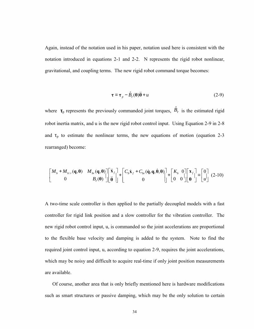
Lew and Moon [35-38] have recently considered the more general case of a robot

attached to a passive compliant base, but only allow three degrees of freedom of base

translation. The scheme compensates for base vibration while following a desired

position. Real-time estimates of the nonlinear rigid body dynamics are computed from

joint accelerations calculated from measured optical encoder position data. The coupled

rigid body equation of motion (last row of equation 2-3) can be written as:

( ) ( , , , ) (2-8)B Nτ + =θ θ θ θ q q τ&& & &

34

Again, instead of the notation used in his paper, notation used here is consistent with the

notation introduced in equations 2-1 and 2-2. N represents the rigid robot nonlinear,

gravitational, and coupling terms. The new rigid robot command torque becomes:

� ( ) (2-9)p B uτ= − +τ τ θ θ&&

where ττττp represents the previously commanded joint torques, �Bτ is the estimated rigid

robot inertia matrix, and u is the new rigid robot control input. Using Equation 2-9 in 2-8

and τp to estimate the nonlinear terms, the new equations of motion (equation 2-3

rearranged) become:

/ ( , ) ( , ) 0( , , , ) 0(2-10)

0 ( ) 0 0 0f fb b r br bb f brM M M KC C

B uτ

+ + + + =

x xq θ q θ x q q θ θθ θθ

&&& &&

&&

A two-time scale controller is then applied to the partially decoupled models with a fast

controller for rigid link position and a slow controller for the vibration controller. The

new rigid robot control input, u, is commanded so the joint accelerations are proportional

to the flexible base velocity and damping is added to the system. Note to find the

required joint control input, u, according to equation 2-9, requires the joint accelerations,

which may be noisy and difficult to acquire real-time if only joint position measurements

are available.

Of course, another area that is only briefly mentioned here is hardware modifications

such as smart structures or passive damping, which may be the only solution to certain

35

problems. One example may be if the controlled motion is fully prescribed and no

deviation is allowed for path modifications or to damp the vibration. Another example

would be if the vibration is not controllable at the point of interface with the rigid robot

or if the vibration is not observable (the micromanipulator or sensors can only be placed

at a node point). Other cases could occur when the vibration controller is designed based

on a reduced order model and fails to compensate for excitation of higher modes in the

system. In these cases, another option may be to introduce a dissipation mechanism to

enhance damping rather than modify the control loop [9,10].

2.6 Limitations of Previous Research

Control of macro/micromanipulators has been investigated using many different

techniques. As noted previously, inertial damping schemes using the micromanipulator

to damp the vibration is an attractive compromise between control system complexity and

system performance. These schemes have been developed and demonstrated for a very

specialized class of systems in unique configurations. Some of the limitations of the

research performed so far in this area are:

1. Full macromanipulator flexibility (translational and rotational) has not been

considered. Lew and Moon [35-38] have taken the more general approach of considering

the macromanipulator as a compliant base, but limit the motion to only translational

motion, which greatly simplifies the problem. The space robotics work by Yoshida et al

[92,93] considers the case of a robot mounted on a floating base and has lent some

valuable theoretical work to this area, but detailed work is yet to be seen.

36

2. The variation in performance throughout the workspace has not been fully

addressed. In particular, there are locations in the workspace where the ability of the

manipulator to generate effective interaction forces and torques is diminished. There has

been some work in space robotics by Torres et al [77,78] and Vliet [80] that begins to

address this issue. A rigorous investigation of these singularities, similar to the work

done by Papadopoulos and Dubowsky [56] for space dynamic singularities, is lacking. In

addition, there has not been a method proposed to address how to use the variation in

performance to improve the effectiveness of the damping scheme.

3. Most of the above schemes have assumed ideal system modeling for development

of the vibration control scheme. Lew and Moon [35-38] looked at estimating nonlinear

and coupling effects but practical implementation of this method could become

challenging. There still needs to be a detailed investigation of the coupled system model

as well as an evaluation of the robustness of the control scheme to modeling errors.

4. Few hardware demonstrations have been performed on realistic

macro/micromanipulators. Those that have been were on robots in specific

configurations and with only one or two vibrational degrees of freedom. In addition, the

only two degree of freedom demonstrations have been on robots that have naturally

decoupled inertial damping performance. The effects of (1-3) may become even more

important with additional degrees of freedom.

5. Methods to maximize the amount of damping provided by the vibration controller

have not been addressed. In addition, practical limitations such as actuator saturation and

limits on joint travel have not been addressed. In fact, very little guidance is available on

37

choosing the vibration control gains or establishing limits on gains that consider these

factors.

6. The impact of the vibration damping controller on the position controller has not

been systematically analyzed. Some researchers have chosen to consider the vibration

problem separately [12,15,63,81,93] while others have carefully chosen the position

control and vibration control loops to have time scale separation [11,33,35].

Of course, there is plenty of room for additional work in this area. This dissertation

seeks to address some of the major issues remaining in the field. In particular, this

research includes:

1. Consideration of the multi-degree of freedom (DOF) macro/micromanipulator

control problem by studying the analogous problem of a rigid robot mounted on a flexible

base.

2. Investigation of the variation in performance throughout the workspace and

inertial singularities, or locations in the workspace where the rigid robot loses its ability

to create effective interactions in one or more degrees of freedom.

3. Development of a control scheme that provides active base vibration damping in

parallel with position control and establishment of appropriate vibration control gain

limits.

4. Simulation and experimental work on a realistic multi-degree of freedom

macro/micromanipulator.

38

CHAPTER III

FLEXIBLE BASE MANIPULATOR MODELING

3.1 Introduction

This chapter describes modeling of a rigid robot mounted on a flexible base. The

flexible base represents a multi-link macromanipulator with locked joints. The rigid

robot will provide the fine-tuned end point position control. In this research, it is also

used to damp vibration in the flexible base. Thus, it is especially important to

characterize the dynamic interactions between the macro and micromanipulator and in

order to do this the system needs to be modeled.

First, a recursive Lagrangian approach is described which is used to model the

macromanipulator. This approach is commonly used in flexible robot modeling and

hence is only briefly reviewed here. Next, the micromanipulator model is developed

using a recursive Newton-Euler algorithm. The important dynamic effects that need to be

characterized are the required joint torques to operate the robot and the interaction forces

and torques acting at the base of the robot. The joint torque equations are the same form

as those for a fixed base rigid robot with additional coupling terms due to the base

motion. The interaction forces and torques are explicitly solved for and are the subject of

39

further investigation in Chapter 4. Chapter 5 then investigates how to control these

interactions to damp the base vibration.

3.2 Flexible Base Model

The flexible base represents a multi-link flexible manipulator with locked joints. The

method chosen here is a recursive Lagrangian formulation using a finite number of

assumed modes, which is applicable to an n-DOF flexible link manipulator. The

advantage of this method is its ability to include flexible link deformation. This method

is well documented and more detailed descriptions may be found in the paper by Book

[8] and others who have used this method to model flexible manipulators [15,32,34,42,

52,53,62,72]. However, other methods may be used provided they yield inertia and

stiffness properties and adequately capture the significant dynamics of the

macromanipulator. Modal damping estimates are also often added and could be based on

experimental results or estimated from material properties.

The key difference between a flexible and rigid robot is its continuous nature. Both

rigid joint motion and elastic deflections govern the motion of a flexible robot, so it

theoretically has an infinite number of degrees of freedom. However, it is necessary to

develop a more manageable model that approximates the system, yet adequately captures

the significant dynamics. The approach described here begins with assuming an

appropriate number of modes to model the flexibility in each link for each degree of

freedom. The position of an arbitrary point on each link is composed of summations of

the assumed mode shapes multiplied by the generalized coordinates. These are used to

40

form the kinetic and potential energy of the system and with Lagrange�s equations yield

the equations of motion of the system. It is assumed for this work the resulting

macromanipulator model can be linearized about an operating point, i.e. at a fixed joint

configuration and neglecting the flexible generalized coordinates in the inertia, stiffness,

and damping matrices. It is further assumed the flex model is developed referenced to an

inertial coordinate frame coincident with its last link, or at the base of the

micromanipulator. The resulting matrices, although constant at a given locked joint

configuration, will generally be fully coupled and the generalized coordinates will only

include the flexible states.

It is assumed each link could have two degrees of freedom of transverse vibration

plus torsion about the z-axis (Figure 3-1) and that axial vibration is negligible. Thus,

there will be a total of 3

1 1

n

i ki k

m= =∑ ∑ equations of motion and generalized coordinates,

where n is the number of macromanipulator links, k represents vibration in the x, y, or θz

direction, and mik is the number of assumed modes for the kth direction of vibration of the

ith link.

3.2.1 Assumed Modes

The first task is to assume an appropriate set of modes for each degree of freedom.

The mode shapes could be based on many methods, such as Ritz series, finite element

models, or analytical results for continuous systems [24]. The chosen set of modes only

needs to be linearly independent and satisfy the system geometric boundary conditions

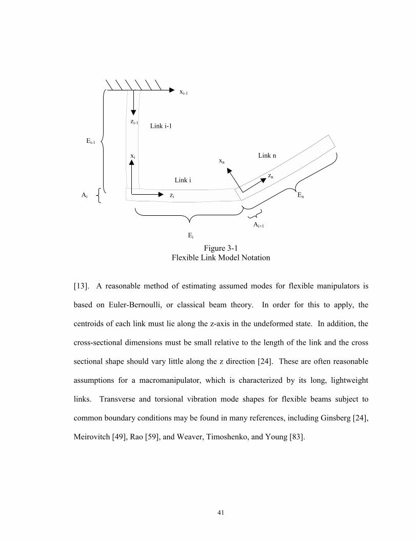
41

Figure 3-1 Flexible Link Model Notation

[13]. A reasonable method of estimating assumed modes for flexible manipulators is

based on Euler-Bernoulli, or classical beam theory. In order for this to apply, the

centroids of each link must lie along the z-axis in the undeformed state. In addition, the

cross-sectional dimensions must be small relative to the length of the link and the cross

sectional shape should vary little along the z direction [24]. These are often reasonable

assumptions for a macromanipulator, which is characterized by its long, lightweight

links. Transverse and torsional vibration mode shapes for flexible beams subject to

common boundary conditions may be found in many references, including Ginsberg [24],

Meirovitch [49], Rao [59], and Weaver, Timoshenko, and Young [83].

Ei-1

Ai

Link i-1

Link i

Link n

xi-1

Ei

Ai+1

xn

En

zi-1

xi

zi

zn

42

The governing differential equation of motion for transverse vibration of a uniform

beam [83] is:

4 2

4 2

( , ) ( , ) 0 (3 -1 )u z t u z tE I Az z

ρ∂ ∂+ =∂ ∂

u(z,t) describes the resulting vibration in the x direction (or v(z,t) in the y direction), as

defined in Figure 3-1, for the ith link. E is modulus of elasticity, ρ is mass density, A is

the cross-sectional area and I is the moment of inertia of the link about the x or y axis (all

assumed constant). Using separation of variables,

1

( , ) ( ) ( ) (3-2)ikm

jj

u z t z T tφ=

=∑

a basis set of mode shape functions can be found of the form:

1 2 3 4sin( ) cos( ) sinh( ) cosh( ) (3-3)j j j j j j j j jC z C z C z C zφ β β β β= + + +

Cjs and βjs are determined from the eigenvalue problem appropriate for the system�s

boundary conditions. mik should be truncated to a reasonable number of modes to

adequately model the flexible dynamics without unnecessarily increasing model size and

complexity. Some researchers have found that two or three modes suffice to represent

flexible dynamics on relatively uncomplicated systems [13], based on the low amplitude

of the higher frequency modes.

Common boundary conditions used for modeling flexible manipulators are fixed/free

or pinned-pinned, but other boundary conditions may be more applicable depending on

the specific application. For example, fixed/free boundary conditions are:

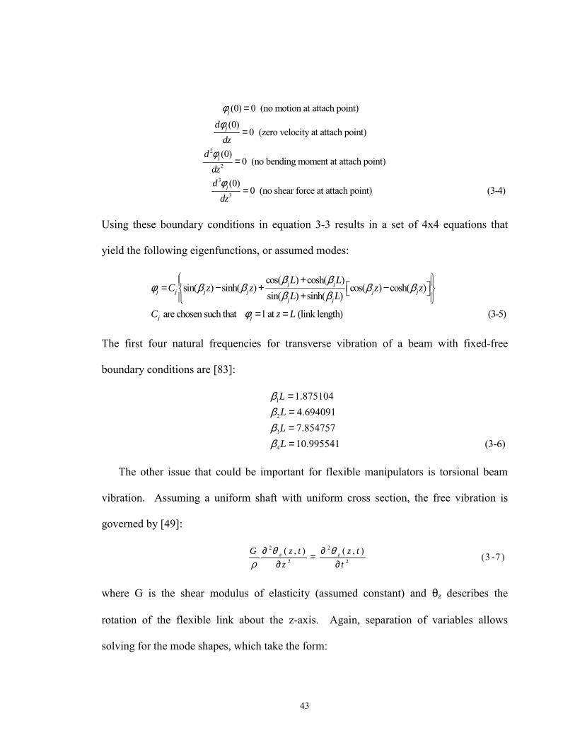
43

2

2

3

3

(0) 0 (no motion at attach point)

(0) 0 (zero velocity at attach point)

(0)0 (no bending moment at attach point)

(0) 0 (no shear force at attach point)

j

j

j

j

ddz

ddzd

dz

φφ

φ

φ

=

=

=

= (3-4)

Using these boundary conditions in equation 3-3 results in a set of 4x4 equations that

yield the following eigenfunctions, or assumed modes:

cos( ) cosh( )sin( ) sinh( ) cos( ) cosh( )

sin( ) sinh( )

are chosen such that 1 at (link length)

j jj j j j j j

j j

j j

L LC z z z z

L L

C z L

β βφ β β β β

β β

φ

+ = − + − + = = (3-5)

The first four natural frequencies for transverse vibration of a beam with fixed-free

boundary conditions are [83]:

1

2

3

4

1.8751044.6940917.85475710.995541 (3-6)

LLLL

ββββ

====

The other issue that could be important for flexible manipulators is torsional beam

vibration. Assuming a uniform shaft with uniform cross section, the free vibration is

governed by [49]:

2 2

2 2

( , ) ( , ) (3 -7 )z zG z t z tz t

θ θρ∂ ∂=

∂ ∂

where G is the shear modulus of elasticity (assumed constant) and θz describes the

rotation of the flexible link about the z-axis. Again, separation of variables allows

solving for the mode shapes, which take the form:

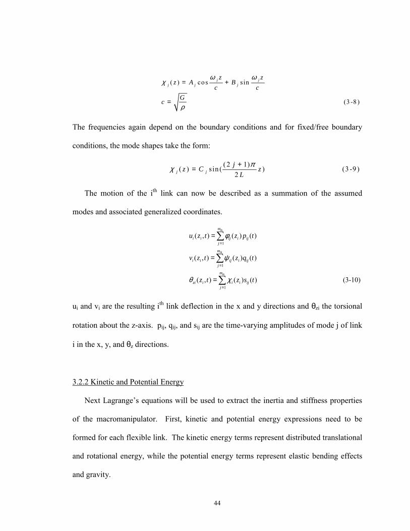
44

( ) co s sin

(3 -8 )

j jj j j

z zz A B

c cGc

ω ωχ

ρ

= +

=

The frequencies again depend on the boundary conditions and for fixed/free boundary

conditions, the mode shapes take the form:

( 2 1)( ) sin ( ) (3 -9 )

2j jjz C z

Lπχ +=

The motion of the ith link can now be described as a summation of the assumed

modes and associated generalized coordinates.

1

1

1

( , ) ( ) ( )

( , ) ( ) ( )

( , ) ( ) ( ) (3-10)

ik

ik

ik

m

i i ij i ijj

m

i i ij i ijj

m

zi i i i ijj

u z t z p t

v z t z q t

z t z s t

φ

ψ

θ χ

=

=

=

=

=

=

∑

∑

∑

ui and vi are the resulting ith link deflection in the x and y directions and θzi the torsional

rotation about the z-axis. pij, qij, and sij are the time-varying amplitudes of mode j of link

i in the x, y, and θz directions.

3.2.2 Kinetic and Potential Energy

Next Lagrange�s equations will be used to extract the inertia and stiffness properties

of the macromanipulator. First, kinetic and potential energy expressions need to be

formed for each flexible link. The kinetic energy terms represent distributed translational

and rotational energy, while the potential energy terms represent elastic bending effects

and gravity.

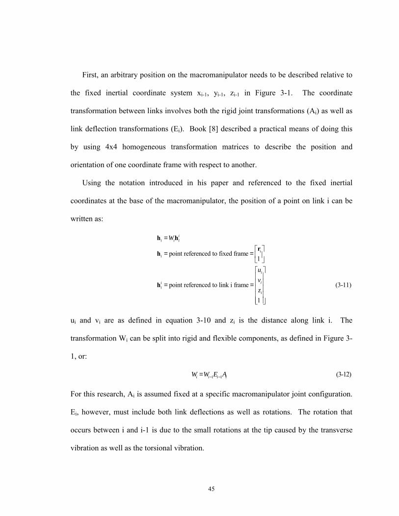
45

First, an arbitrary position on the macromanipulator needs to be described relative to

the fixed inertial coordinate system xi-1, yi-1, zi-1 in Figure 3-1. The coordinate

transformation between links involves both the rigid joint transformations (Ai) as well as

link deflection transformations (Ei). Book [8] described a practical means of doing this

by using 4x4 homogeneous transformation matrices to describe the position and

orientation of one coordinate frame with respect to another.

Using the notation introduced in his paper and referenced to the fixed inertial

coordinates at the base of the macromanipulator, the position of a point on link i can be

written as:

ipoint referenced to fixed frame1

point referenced to link i frame (3-11)

1

ii i i

i

i

iii

i

W

uvz

=

= =

= =

h hr

h

h

ui and vi are as defined in equation 3-10 and zi is the distance along link i. The

transformation Wi can be split into rigid and flexible components, as defined in Figure 3-

1, or:

1 1 (3-12)i i i iW W E A− −=

For this research, Ai is assumed fixed at a specific macromanipulator joint configuration.

Ei, however, must include both link deflections as well as rotations. The rotation that

occurs between i and i-1 is due to the small rotations at the tip caused by the transverse

vibration as well as the torsional vibration.

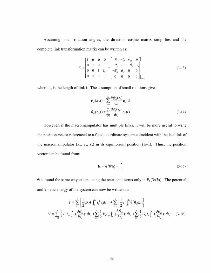
46

Assuming small rotation angles, the direction cosine matrix simplifies and the

complete link transformation matrix can be written as:

0 1 0 0 00 1 0 0 0

(3-13)0 0 1 0 00 0 0 1 0 0 0 0

i

zi yi i

zi xi ii

i yi xi

z L

uv

El

θ θθ θθ θ

=

− = + −

where Li is the length of link i. The assumption of small rotations gives:

1

1

( )( , ) ( )

( )( , ) ( ) (3-14)

i

i

mij i

xi i ijj i

mij i

yi i ijj i

zz t q t

zz

z t p tz

ψθ

φθ

=

=

∂≈

∂∂

≈∂

∑

∑

However, if the macromanipulator has multiple links, it will be more useful to write

the position vector referenced to a fixed coordinate system coincident with the last link of

the macromanipulator (xn, yn, zn) in its equilibrium position (E=I). Thus, the position

vector can be found from:

1 (3-15)1

iii i i iA W−

= =

rh h

θθθθ is found the same way except using the rotational terms only in Ei (3x3s). The potential

and kinetic energy of the system can now be written as:

0 0

1 1

2 2 2

0 0 01 1 1

1 1 2 2

1 1 1( ) ( ) ( ) (3-16)2 2 2

i i

i i i

n nL LT Ti i i i i i i i i

i i

n n nL L Lyixi zii xi i i yi i i i i

i i ii i i

T A dz I dz

V E I dz E I dz G J dzz z z

ρ

θθ θ= =

= = =

= + ∂∂ ∂= + +

∂ ∂ ∂

∑ ∑∫ ∫

∑ ∑ ∑∫ ∫ ∫

r r θ θ& && &

47

where:

x y

mass densitycross-sectional area

E modulus of elasticityI , I area moment of inertia of the cross sectional area computed about the x or y axis

G modulus of rigidityJ polar area moment of the cros

Aρ ===

=

== s sectional area computed about the neutral axis

One of the benefits of this method is that as much detail can be included in the equations

of motion as desired. Here many of the assumptions that have been used and justified by

other researchers have been used to pare the equations of motion down to the most

significant contributions [8,24,34,46,52,72,83].

Now Lagrange's equations can be used to derive the equations of motion.

(3-17)ii i i

d T T Vdt q q q ∂ ∂ ∂− + = ∂ ∂ ∂

Q&

Qi are the nonconservative generalized forces applied to the macromanipulator

corresponding to the generalized coordinate qi. In this research, these are the interaction

forces and torques created by the micromanipulator. The generalized forces are

determined from the virtual work done by the micromanipulator, or

(3-18)IF IFWork rδ δ δθ= +F τ

The infinitesimal displacements and rotations at the tip of the macromanipulator are

given by equation 3-15 evaluated at zi=Li. The partial derivatives of the resulting

infinitesimal displacements and rotations are taken with respect to each generalized

coordinate to find the generalized forces.

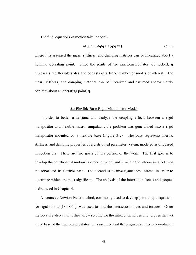
48

The final equations of motion take the form:

( ) ( ) ( ) (3-19)M C K+ + =q q q q q q Q% && % & %

where it is assumed the mass, stiffness, and damping matrices can be linearized about a

nominal operating point. Since the joints of the macromanipulator are locked, q

represents the flexible states and consists of a finite number of modes of interest. The

mass, stiffness, and damping matrices can be linearized and assumed approximately

constant about an operating point, q .

3.3 Flexible Base Rigid Manipulator Model

In order to better understand and analyze the coupling effects between a rigid

manipulator and flexible macromanipulator, the problem was generalized into a rigid

manipulator mounted on a flexible base (Figure 3-2). The base represents inertia,

stiffness, and damping properties of a distributed parameter system, modeled as discussed

in section 3.2. There are two goals of this portion of the work. The first goal is to

develop the equations of motion in order to model and simulate the interactions between

the robot and its flexible base. The second is to investigate these effects in order to

determine which are most significant. The analysis of the interaction forces and torques

is discussed in Chapter 4.

A recursive Newton-Euler method, commonly used to develop joint torque equations

for rigid robots [18,48,61], was used to find the interaction forces and torques. Other

methods are also valid if they allow solving for the interaction forces and torques that act

at the base of the micromanipulator. It is assumed that the origin of an inertial coordinate

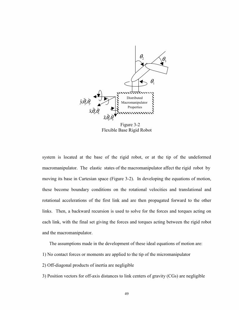
49

Figure 3-2 Flexible Base Rigid Robot

system is located at the base of the rigid robot, or at the tip of the undeformed

macromanipulator. The elastic states of the macromanipulator affect the rigid robot by

moving its base in Cartesian space (Figure 3-2). In developing the equations of motion,

these become boundary conditions on the rotational velocities and translational and

rotational accelerations of the first link and are then propagated forward to the other

links. Then, a backward recursion is used to solve for the forces and torques acting on

each link, with the final set giving the forces and torques acting between the rigid robot

and the macromanipulator.

The assumptions made in the development of these ideal equations of motion are:

1) No contact forces or moments are applied to the tip of the micromanipulator

2) Off-diagonal products of inertia are negligible

3) Position vectors for off-axis distances to link centers of gravity (CGs) are negligible

Distributed Macromanipulator

Properties , ,y yyθ θ&& &&&

, ,x xxθ θ&& &&&, ,z zzθ θ&& &&&

1θ

2θ3θ

50

4) Friction effects and other nonlinearities are not modeled

5) Rotor inertia effects are not included.

If actuator dynamics dominate the rigid robot performance, an alternate form of the rigid

robot model may apply. However, the interaction forces and torques described by this

model will still be valid.

First, consider for the moment a single link rigid robot mounted to a flexible base.

The base is free to move in any direction. The arm rotates about the x-axis as defined in

Figure 3-3 (out of the page).

Figure 3-3 Flexible Base Single Link Rigid Robot

The acceleration of the center of gravity of the link is given by:

0

0

( )w h e re :

�� � ( )�� �( )�� �( ) (3 -2 0 )

G C G C G

x y z

x y z

x i y j z g k

i j k

i j k

θ θ θ θ

θ θ θ θ

= + × + × ×

= + + +

= + + +

= + + +

a a α r ω ω r

a

ω

α

&& && &&

& & & &

&& && && &&

θ

xxx θθ &&&&& ,,

yyy θθ &&&&& ,,

, ,z zz θ θ& &&&&

51

where: aG = acceleration of the center of gravity of the rigid link a0 = acceleration of the base g = gravitational constant ωωωω = angular velocity of the link αααα = angular acceleration of the link rCG = position vector from the base to the center of gravity of the link

Now the interaction forces and torques at the base of the link can be solved for:

( )

( 3 -2 1 )

I F G

x x x

IF C G I F y y y

z z z

m

I

I

I

θ θθ

θ

=

+

= − × +

F a

τ r F

&& &&

&&

&&

where m is the mass of the robot arm and Ixx, Iyy, and Izz are moments of inertia of the link

about the respective axes. Just for this one link case, the interaction forces take the form:

2

1 0 0 0 0 0 0 0 00 1 0 0 00 0 1 0 0

x

y

IFxz

IFy

IFz

x rc rsy rc rc rs rs

F z rs rs rcF mF

θθ θθ θ θ θ θ θ θθ θ θθ

− − + + + − + − =

&&&&&& && &&&

&& &&

2

2

2

0 0

0 0 0 0 2 0 0

0 0 2 0 0

x

y

z

x y

x z

y z

rsrc rc

rs rc rs rcrc rsrs rc

θθ θ

θ θ θ

θ θθ θ θ θθ θ θ θθ θθ θ

−

− − + − + −

&

&

&

& & &

& &

& &

(3-22)0

+ 0 g

x

y

z

θ θθ θ

θ θ

&

& &

& &

Here the abbreviated form for the trigonometric functions, cθ and sθ, are used to

represent cosθ and sinθ, as will be the case for the remainder of this document. Using the

notation for the macromanipulator in the previous section and equations 3-10 and 3-14,

the displacements and rotations at the tip of the macromanipulator can be written in terms

52

of the generalized coordinates, q. Thus, these equations can be written in more compact

form as:

1 22 2

0 0 0 0 1 00 2

( ) ( ) ( ) ( ) ( , ) ( ) (3-23)

( ) ( ) ( ) ( ) ( )( , )f f f fc fc fIF

IF c c

C B N N N GFC B N N GNτ τ τ τ ττ

θ θ θ θ θ θ θθ

τ θ θ θ θ θθ θ θ

= + + + +

qq q

&&&& & &

&& &

The goal of the control scheme is to control the interaction forces and torques via the

rigid robot to damp vibration in the macromanipulator. From the above reduced

equations of motion, it is apparent the effects that directly influence the interaction forces

and torques are given by:

2

0 0

( ) ( ) (3-24)

( ) ( )f fIF

IF

B NFB Nτ τ

θ θθ θ

τ θ θ

= +

&& &

The generic algorithm is similar to the well-documented Newton-Euler method for

deriving the equations of motion for a rigid robot, except in this case the interaction

forces and torques are required in addition to the joint torque equations. The notation

used below is consistent with that found in Sciavicco and Siciliano [61] where the more

efficient method of referring the vectors to the current frame associated with link i is

used. The algorithm uses forward recursions, which propagate the velocities and

accelerations of each link forward to the next link. This is followed by backward

recursions, which solve for the forces and torques acting on each link starting with the

force and moment applied to the end effector (assumed zero for this work).

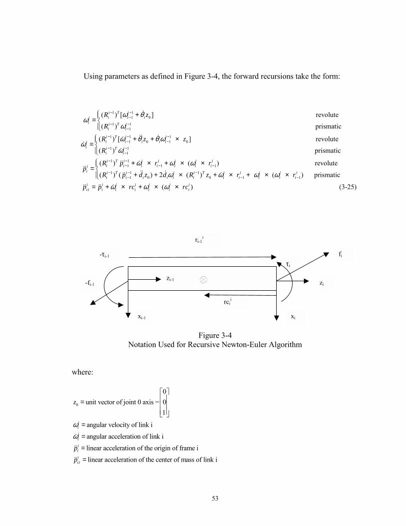
53

Using parameters as defined in Figure 3-4, the forward recursions take the form:

1 11 0

1 11

( ) [ ] revolute

( )

i T ii i ii

i i T ii i

R z

R

ω θω

ω

− −−

− −−

+=

&

1 1 11 0 1 0

1 11

prismatic

( ) [ ] revolute

( )

i T i ii i i i ii

i i T ii i

R z z

R

ω θ θωω

ω

− − −− −

− −−

+ + ×=

&& &&&

&

1 11 1 1

prismatic

( ) ( )

i T i i i i i ii i i i i i ii

i

R p r rp

ω ω ω− −− − −

+ × + × ×=

&& &&&

1 1 11 0 0 1 1

revolute

( ) ( ) 2 ( ) ( ) prismatic

( )

i T i i i T i i i i ii i i i i i i i i i i

i i i i i i ici i i i i i i

R p d z d R z r r

p p rc rc

ω ω ω ω

ω ω ω

− − −− − −

+ + × + × + × ×= + × + × ×

&& &&& &

&& && & (3-25)

Figure 3-4 Notation Used for Recursive Newton-Euler Algorithm

where:

0

0unit vector of joint 0 axis = 0

1

angular velocity of link i

angular acceleration of link i

linear acceleration of the origin of frame i

linear acceleration of the center

iiiiiiici

z

pp

ωω

=

=

=

=

=

&

&&

&& of mass of link i

rcii

xi-1

zi-1

xi

zi

fi

-fi-1

τi

-τi-1

ri-1i

54

The backward recursions take the form:

1

1 1

10

10

i

( ) revolute

( ) prismaticinteraction force between links i and i-1

int

i ii i i i i ci

i i i i i i iIFi i i IFi i i i i i i i i i i i

T i TIFi i

i T i TI i

i

IF

f R f m pR R f rc f rc I I

R zf R z

f

τ τ ω ω ω

ττ

τ

+ +

+ + + +

−

−

= +

= + × − × + + ×

=

==

&&

&

eraction torque between links i and i-1generalized joint actuation torque for link i (3-26)iτ =

Boundary conditions of the tip velocities and accelerations of the macromanipulator are

applied to the first link and propagated through the forward recursions. It is assumed that

the micromanipulator is not in contact with any object so the forces and torques applied

to the tip of its last link are zero.

The equations of motion take the general form:

0 0 0 0

( ) ( , ) ( ) ( , , , )

( ) ( , ) ( ) ( , , , )

( ) ( , ) ( ) ( , , , )

IF f f i j f fc

IF i j c

i j c

B N C N

B N C N

B N C Nτ τ τ τ

τ τ τ τ

= + + +

= + + +

= + + +

F θ θ θ θθ θ q q q θ θ

τ θ θ θ θ θ θ q q q θ θ

τ θ θ θ θ θ θ q q q θ θ

&& & & &&& &

&& & & &&& &

&& & & &&& & (3-27)

θθθθ represents the rigid robot joint variables and q represents the flexible base generalized

coordinates. Bf, Bτ0, Cf, and Cτ0 represent inertia effects of the micro and macro

manipulators, respectively. Bf and Bτ0 are particularly important because they represent

the controllable rigid robot inertia effects. These matrices are, in general, not symmetric,

or positive definite (but the inertia matrix for the complete coupled system is, of course).

The remaining terms in 3-27 represent nonlinear and gravitational effects. The third

equation is the typical joint torque equation with extra coupling terms. Often actuator

dynamics or other effects dominate the robot performance, so this equation could take

55

other forms. However, for this work it is assumed the relationship between the joint

actuation torques and joint positions is known and controllable.

These equations were written in symbolic form in Matlab [21]. The

macromanipulator tip angular velocities, angular accelerations, and translational

accelerations are the boundary conditions and are given by:

0 0 00 0 0, , (3-28)

x x

y y

z z

xp y

g z

ω ωω ω ω ω

ω ω

= = = +

& &&

& & && &&

&&&

These were used in equation 3-25 and propagated forward to each link, and then

equations 3-26 were used to find the interaction forces and torques and joint actuation

torques. These equations were developed for anthropomorphic, spherical, wrist, and

anthropomorphic/wrist robot configurations and many are included in Appendix A. The

ability of this method to predict the interaction forces and torques was verified

experimentally with a six-degree-of freedom force/torque sensor mounted at the base of a

three DOF anthropomorphic rigid robot.

3.4 Coupled Macro/Micromanipulator Model

The micromanipulator is considered in this work to apply the interaction forces and

torques to the flexible base. The flexible manipulator, given by equation 3-19, is now

written with translational and rotational effects considered separately. The generalized

forces applied by the micromanipulator are given by 3-18. Here, for the sake of

generality, the interactions are assumed applied directly to the flexible base. In this case,

the flexible manipulator equations of motion become:

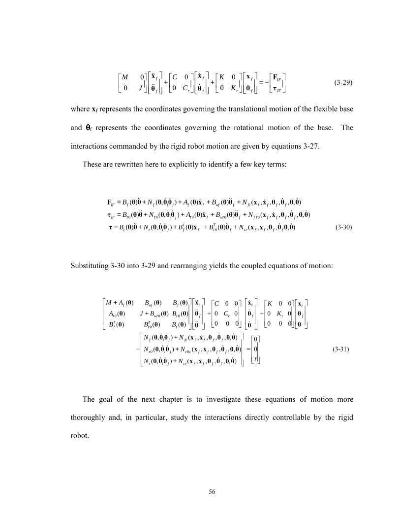
56

0 0 0 (3-29)

0 00f f f IF

r r f IFf f

C KMC KJ

+ + = −

x x x Fθ τθ θ

&& &

&& &

where xf represents the coordinates governing the translational motion of the flexible base

and θθθθf represents the coordinates governing the rotational motion of the base. The

interactions commanded by the rigid robot motion are given by equations 3-27.

These are rewritten here to explicitly to identify a few key terms:

0 0 0 0 0

0

( ) ( , ) ( ) ( ) ( , , , , , )

( ) ( , ) ( ) ( ) ( , , , , , )

( ) ( , ) ( )

IF f f i j f f wf f fc f f f f

IF i j f w f f f f f f

i j f f

B N A B N

B N A B N

B N B Bτ τ τ τ τ

ττ τ τ

= + + + +

= + + + +

= + + +

F θ θ θ θ θ θ x θ θ x x θ θ θ θ

τ θ θ θ θ θ θ x θ θ x x θ θ θ θ

τ θ θ θ θ θ θ x

&& & & && & &&& &

&& & & && & &&& &

&& & & && ( ) ( , , , , ) (3-30)Tf c f f f fNτ+θ θ x x θ θ θ θ&& & &&

Substituting 3-30 into 3-29 and rearranging yields the coupled equations of motion:

f f f

0 0 0

0

( ) ( ) ( ) 0 0 0 0 ( ) ( ) ( ) + 0 0 + 0 0

0 0 0 0 0 0 ( ) ( ) ( )

f wf f

w f r f rT

f

M A B B C KA J B B C KB B Bτ τ ττ

τ τ

+ +

x xθ θ θ xθ θ θ θ θθ θ θ θ θ

&& &

&& &

&& &

0 0

( , ) ( , , , , , ) 0 + ( , ) ( , , , , , ) = 0

( , ) ( , , , , , )

f

f i j fc f f f f

i j c f f f f

i j c f f f f

N N

N N

N Nτ τ

τ ττ

+ + +

θθ

θ θ θ x x θ θ θ θ

θ θ θ x x θ θ θ θ

θ θ θ x x θ θ θ θ

& & & &&

& & & &&

& & & &&

(3-31)

The goal of the next chapter is to investigate these equations of motion more

thoroughly and, in particular, study the interactions directly controllable by the rigid

robot.

57

CHAPTER IV

INTERACTION FORCES AND TORQUES AND INERTIAL SINGULARITIES

4.1 Introduction

This chapter addresses the interaction forces and torques acting between the rigid

robot and its flexible base. Recall these are given by:

0 0 0 0

( ) ( , ) ( ) ( , , , )

( ) ( , ) ( ) ( , , , ) (4-1)IF f f i j f fc

IF i j c

B N C N

B N C Nτ τ τ τ

= + + +

= + + +

F θ θ θ θ θ θ q q q θ θ

τ θ θ θ θ θ θ q q q θ θ

&& & & &&& &

&& & & &&& &

The focus of this chapter is the directly controllable rigid robot effects, or those terms that

are only functions of θθθθ (the first two terms in each equation). For completeness, the more

detailed equations of motion for each robot may be found in Appendix A

(anthropomorphic, spherical, wrist, and anthropomorphic/wrist robots). The notation and

coordinate systems used are shown in Figures 4-1 through 4-4. The robot configurations

are defined consistent with those described in Sciavicco and Siciliano [61] for

anthropomorphic and spherical arm robots and spherical wrist robots, with one exception

noted in Figure 4-1. In addition, terminology consistent with McGill/King [47] will be

used where centripetal refers to accelerations and centrifugal refers to forces.

First, the inertia forces and torques are discussed, or those generated by accelerating

the links of the rigid robot. An important part of this work involved investigating

58

�inertial singularities,� or regions in the workspace where the robot loses its ability to

create inertia interactions in one or more degrees of freedom. These are important

because the control scheme inverts the inertia matrix, which presents a problem when

these matrices become singular. However, these singularities also represent physical

limitations, so it is important to understand where and why they occur and, if possible,

devise ways of avoiding operation in or near these regions.

Next, the nonlinear centrifugal and coriolis forces and torques are discussed. There

are regions in the workspace where these can become large during multi-DOF actuation

of the joints. These effects are driven by the joint space configuration of the robot and

the joint velocities. In most configurations, the ratio of inertia to nonlinear effects is

large. However, in some configurations the nonlinear effects can interfere with the

inertia effects. If the amplitude of joint motion is limited appropriately, this ratio can be

improved. The remainder of the interaction terms involve combined rigid robot and

flexible base coordinates and are not discussed further here other than to note they are

important for accurate modeling. Finally, the interaction forces and torques were

developed using the Newton-Euler method described in chapter 3. However, a more

efficient approach to find the inertia and nonlinear rigid force effects is presented here.

The work presented in this chapter leads to two important conclusions, which will be

used in the development of the control scheme. First, since the inertia effects are

functions of the joint configuration, this variation in performance may be used to ensure

the robot operates in joint space configurations better suited for inertial damping. This is

possible because there are normally multiple inverse kinematic solutions corresponding

59

to a given end point position (provided the robot is not operating at a kinematic

singularity). A performance measure to predict the rigid robot's ability to create effective

multi-DOF inertia interactions is introduced here. It can be used to choose better inverse

kinematic solutions for inertial damping and will become an important part of the

performance index discussed in Chapter 5. Second, if the joint amplitudes are limited

appropriately, the ratio of inertia/nonlinear effects can be improved. The amplitude of

motion can be controlled by establishing proper limits on the vibration control feedback

gains. The control scheme and feedback gains will be discussed in Chapter 5. The

adequacy of these models in predicting the interactions was tested on a three DOF

anthropomorphic robot with a six-axis ATI force/torque sensor mounted to its base.

These results will be presented in Chapter 7.

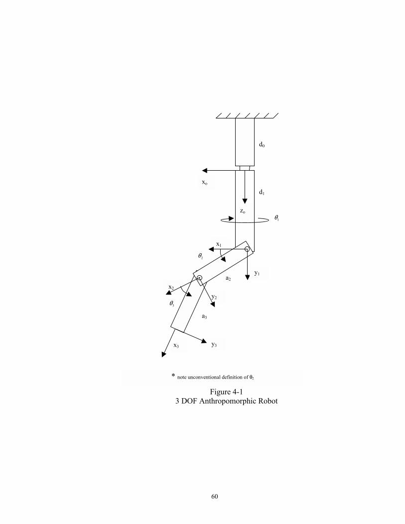
60

Figure 4-1 3 DOF Anthropomorphic Robot

* note unconventional definition of θ2

x1

y2

x2

zo

xo

y1

x3 y3

1θ

2θ

3θ

d0

d1

a2

a3

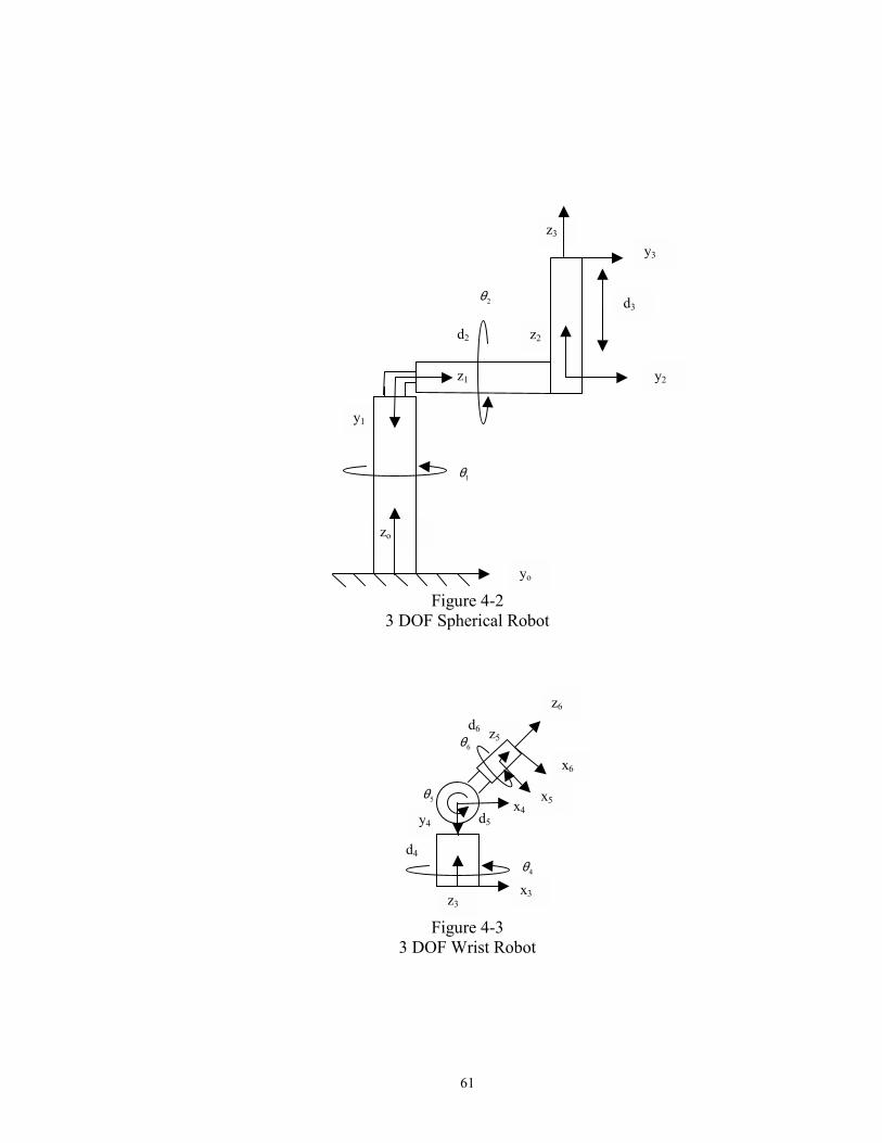
61

Figure 4-2 3 DOF Spherical Robot

Figure 4-3 3 DOF Wrist Robot

z3

z2

z1

y1

zo

yo

d3

y2

y3

1θ

2θ

d2

x4

z3

z5

y4

x3

x5

x6

z6

4θ

5θ

6θ

d4

d5

d6

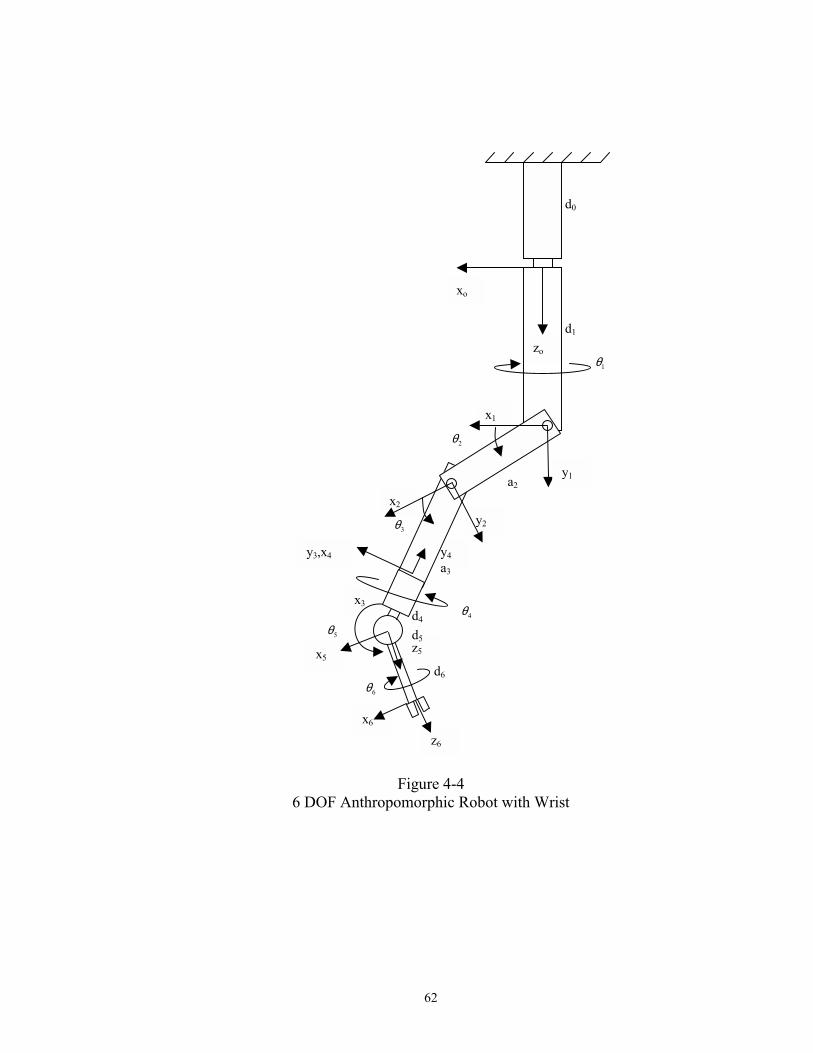
62

Figure 4-4

6 DOF Anthropomorphic Robot with Wrist

z6

z5

x6

x1

x3

y4

y2

x2

zo

xo

y1

y3,x4

x5

1θ

2θ

3θ

4θ

5θ

6θ

d0

d1

a2

a3

d4

d5

d6

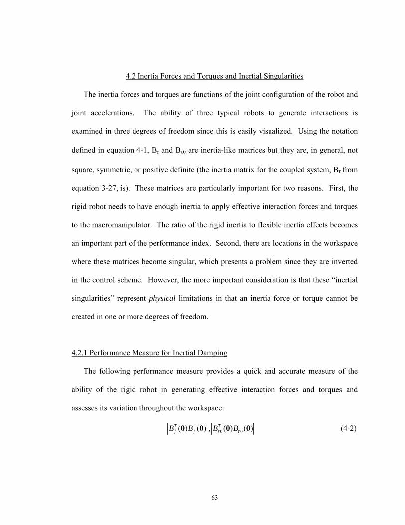
63

4.2 Inertia Forces and Torques and Inertial Singularities

The inertia forces and torques are functions of the joint configuration of the robot and

joint accelerations. The ability of three typical robots to generate interactions is

examined in three degrees of freedom since this is easily visualized. Using the notation

defined in equation 4-1, Bf and Bτ0 are inertia-like matrices but they are, in general, not

square, symmetric, or positive definite (the inertia matrix for the coupled system, Bτ from

equation 3-27, is). These matrices are particularly important for two reasons. First, the

rigid robot needs to have enough inertia to apply effective interaction forces and torques

to the macromanipulator. The ratio of the rigid inertia to flexible inertia effects becomes

an important part of the performance index. Second, there are locations in the workspace

where these matrices become singular, which presents a problem since they are inverted

in the control scheme. However, the more important consideration is that these �inertial

singularities� represent physical limitations in that an inertia force or torque cannot be

created in one or more degrees of freedom.

4.2.1 Performance Measure for Inertial Damping

The following performance measure provides a quick and accurate measure of the

ability of the rigid robot in generating effective interaction forces and torques and

assesses its variation throughout the workspace:

0 0( ) ( ) , ( ) ( ) (4-2)T Tf fB B B Bτ τθ θ θ θ

64

Alternately the combined ability of the robot to generate interaction forces and torques

may be evaluated by assessing:

0

( ) ( )

( ) (4-3)

( )

T

f

B B

BB

Bτ

=

θ θ

θθ

First, it is important to note a few points about these matrices. They are real but not,

in general, square, or symmetric and thus will not have real eigenvalues [73]. However,

BTB will always be symmetric and its determinant will be positive. Singular value

decomposition is a related technique noted for its usefulness in determining how near a

matrix comes to becoming singular. It has also been noted that the use of only the

minimum and maximum singular values is overconservative [23]. Thus, the determinant

of BTB, which is the product of the singular values, was chosen for the performance

measure. In addition, although this dissertation does not specifically address cases of

underactuation or redundancy, the proposed measure may be extended to those cases

since there is no requirement that the matrices be square. Finally, the determinant of a

matrix can much more easily be evaluated than eigenvalues or singular values, which is

particularly important if the performance measure will be used in real-time. This

measure not only provides an indication of how these effects vary throughout the

workspace, but also shows regions where full multi-DOF inertial damping capability is

not possible. The goal here is to use this performance measure to choose robot joint

space locations where the inertia effects are large, whenever possible.

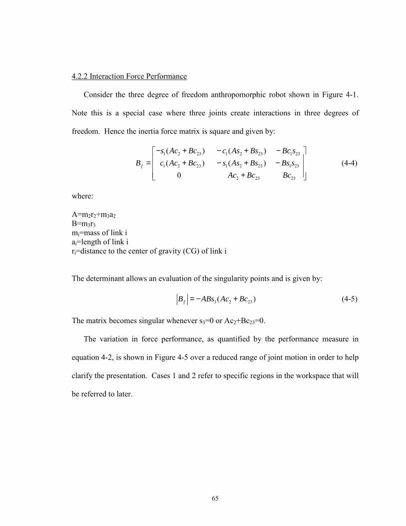
65

4.2.2 Interaction Force Performance

Consider the three degree of freedom anthropomorphic robot shown in Figure 4-1.

Note this is a special case where three joints create interactions in three degrees of

freedom. Hence the inertia force matrix is square and given by:

1 2 23 1 2 23 1 23

1 2 23 1 2 23 1 23

2 23 23

( ) ( ) ( ) ( ) (4-4) 0

f

s Ac Bc c As Bs Bc sB c Ac Bc s As Bs Bs s

Ac Bc Bc

− + − + − = + − + − +

where:

A=m2r2+m3a2 B=m3r3 mi=mass of link i ai=length of link i ri=distance to the center of gravity (CG) of link i

The determinant allows an evaluation of the singularity points and is given by:

3 2 23( ) (4-5)fB ABs Ac Bc= − +

The matrix becomes singular whenever s3=0 or Ac2+Bc23=0.

The variation in force performance, as quantified by the performance measure in

equation 4-2, is shown in Figure 4-5 over a reduced range of joint motion in order to help

clarify the presentation. Cases 1 and 2 refer to specific regions in the workspace that will

be referred to later.

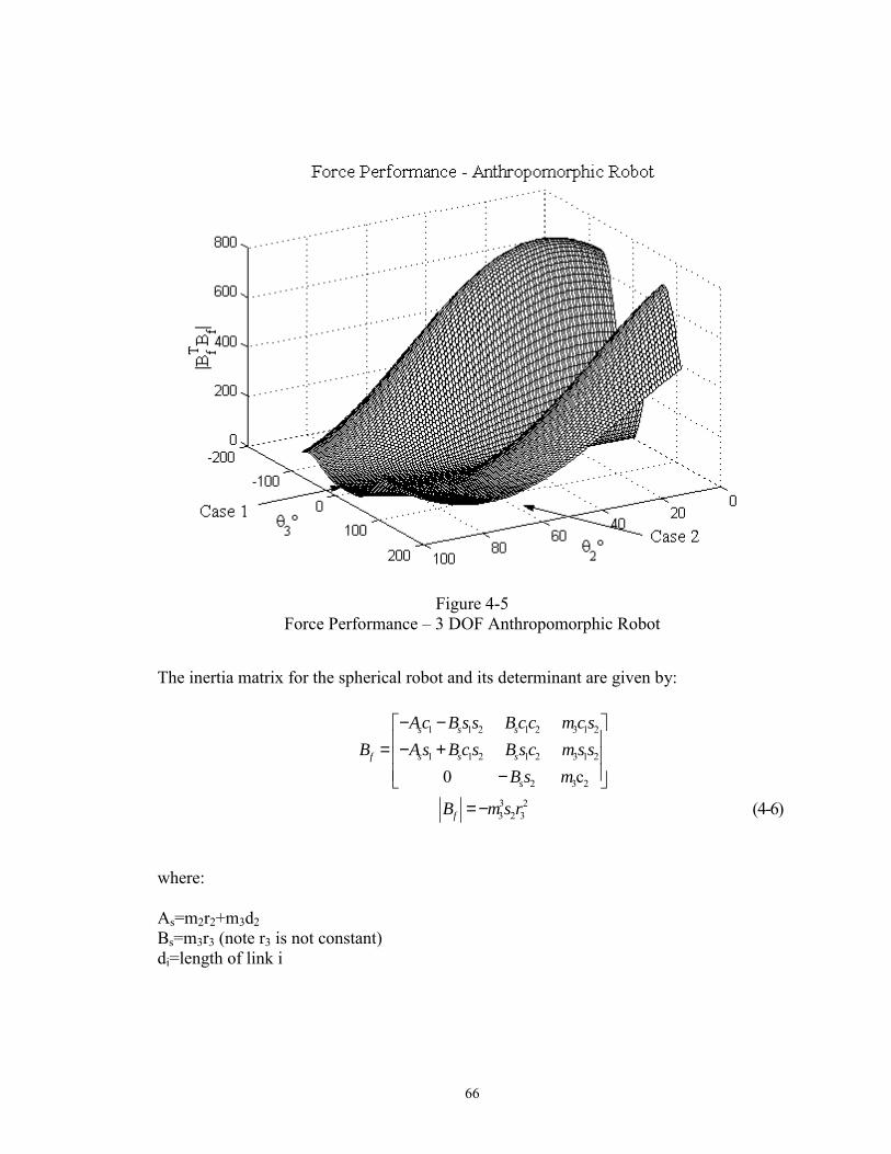
66

Figure 4-5

Force Performance � 3 DOF Anthropomorphic Robot

The inertia matrix for the spherical robot and its determinant are given by:

1 1 2 1 2 3 1 2

1 1 2 1 2 3 1 2

2 3 2

3 23 2 3

0 c

(4-

s s s

f s s s

s

f

Ac B s s B c c m c sB A s B c s B s c m s s

B s m

B m s r

− − = − + −

=− 6)

where: As=m2r2+m3d2 Bs=m3r3 (note r3 is not constant) di=length of link i

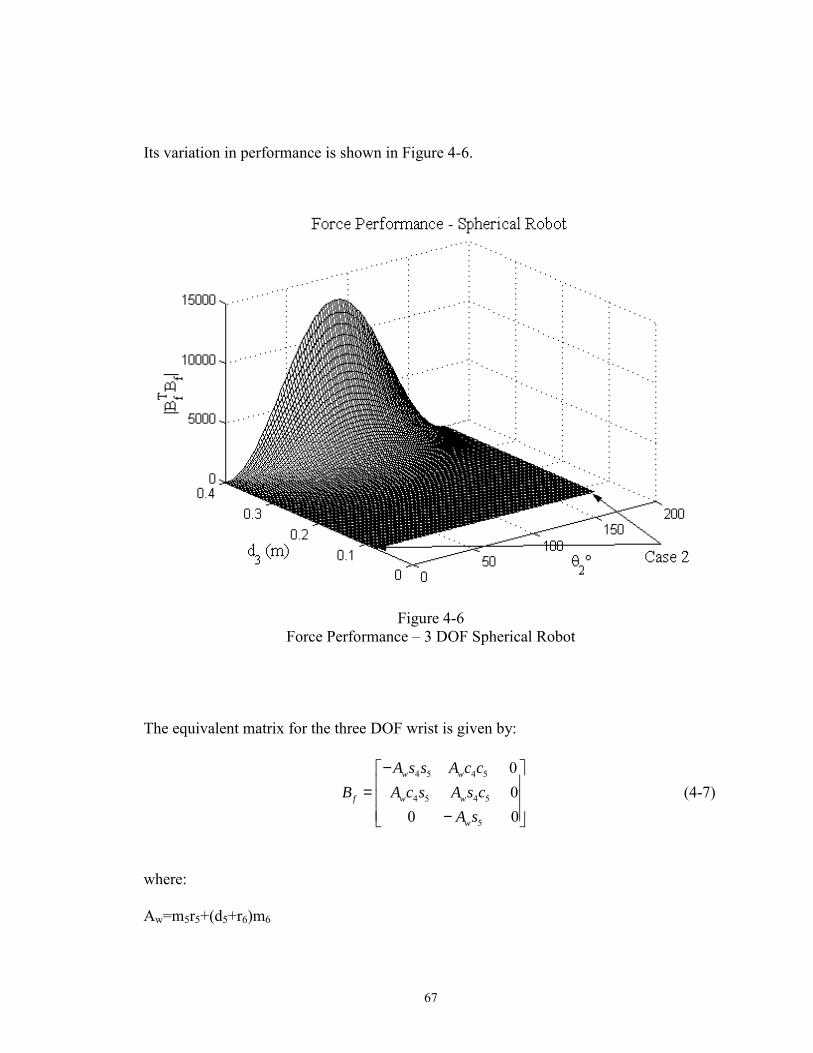
67

Its variation in performance is shown in Figure 4-6.

Figure 4-6

Force Performance � 3 DOF Spherical Robot

The equivalent matrix for the three DOF wrist is given by:

4 5 4 5

4 5 4 5

5

0 0 (4-7) 0 0

w w

f w w

w

A s s A c cB A c s A s c

A s

− = −

where: Aw=m5r5+(d5+r6)m6

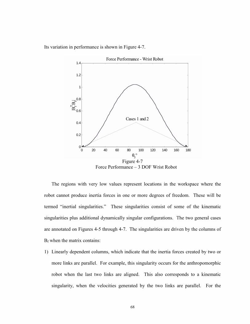
68

Its variation in performance is shown in Figure 4-7.

0 20 40 60 80 100 120 140 160 1800

0.2

0.4

0.6

0.8

1

1.2

1.4Force Performance - Wrist Robot

θ5°

|BfTB f|

Cases 1 and 2

Figure 4-7

Force Performance � 3 DOF Wrist Robot

The regions with very low values represent locations in the workspace where the

robot cannot produce inertia forces in one or more degrees of freedom. These will be

termed �inertial singularities.� These singularities consist of some of the kinematic

singularities plus additional dynamically singular configurations. The two general cases

are annotated on Figures 4-5 through 4-7. The singularities are driven by the columns of

Bf when the matrix contains:

1) Linearly dependent columns, which indicate that the inertia forces created by two or

more links are parallel. For example, this singularity occurs for the anthropomorphic

robot when the last two links are aligned. This also corresponds to a kinematic

singularity, when the velocities generated by the two links are parallel. For the

69

spherical robot, this occurs when joint 2 is at 0° or 180°, when both links 1 and 2

create velocities (and inertia forces) in the horizontal direction. All of the three DOF

spherical robot singularities are the same as the kinematic singularities.

2) A column of zeros, which indicates a location in the workspace where the motion of a

joint cannot create any inertia interaction forces. This singularity occurs when the

CG of the robot is aligned along an axis of rotation. For the anthropomorphic robot,

this occurs when the system CG is aligned along the z-axis, so link 1 can produce no

interaction inertia forces. In the spherical robot, this will occur if link 3 is aligned

along the axis of joint 2, which renders a middle column of zeros. This singularity

can be avoided by requiring some minimum length to link three. These are, in

general, different from the kinematic singularities. The inertial singularities depend

on the location of the CG of the system. If it is known where these occur, they can be

avoided by not operating in those joint space configurations.

In the case of the anthropomorphic and spherical robots, link 1 has no effect on the inertia

force performance because it cannot affect the CG of the system.

Given the configuration shown in Figure 4-3, the wrist is always singular in three

degrees of freedom. Its last link cannot create any inertia interaction forces since its axis

of rotation is along the main link of the robot. In addition, only the orientation of joint 5

affects the inertia forces since it is the only joint that affects the CG of the system. It is

also interesting to note the wrist singularities occur when the arm is straight down or

straight up (θ5=0° or 180°). This is a combination of cases 1 and 2 since these are

kinematic singularities and the CG is aligned along joint 1. Note the extremely small

70

force magnitudes generated by the wrist, indicating its use alone would not be very

effective at creating interactions.

It is also worth mentioning another type of singularity, which corresponds to a row of

zeros in the matrix or two parallel rows. This singularity occurs in conjunction with one

of the other singularity configurations discussed above. For example, if the CG of the

anthropomorphic robot is oriented along the axis of rotation of joint 1 (case 2), an inertia

force cannot be produced in the out-of-plane direction. In this case, two of the rows can

become parallel or one can become a row of zeros, depending on θ1. Two other types of

row singularities can occur in conjunction with the kinematic singularity at θ3=0° (case

1). When joint 2 is at 90° (straight down) and joint 3 is at 0°, no inertia forces can be

produced in the z direction and the third row becomes a row of zeros. Finally the

orientation at θ2=0°, θ3=0° can result in a row of zeros in either the x or y direction,

depending on θ1. These are easily identified using the proposed performance measure

defined in equation 4-2 and serve to further verify the singularities are driven by the

columns of the inertia matrices.

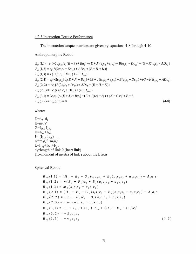
71

4.2.3 Interaction Torque Performance

The interaction torque matrices are given by equations 4-8 through 4-10:

Anthropomorphic Robot:

0 1 2 23 3 2 2 2 3 3 2 3 23 2 2 2

0 1 2 3 23 2

0 1 2 3 23 3

0 1 2 23 3 2 2 2 3 3

(1,1) { 2 [ ( ) ] ( )( ) ( ) ( ) }(1, 2) { (2 ) ( )}(1,3) { ( ) }(2,1) { 2 [ ( ) ] ( )( )

zz

B c c s c E J Ba E J s c s c B a s Dc G K s c ADcB s B a c Ds ADs E H KB s B a c Ds E IB s c s c E J Ba E J s c s c B

τ

τ

τ

τ

= − + + + + + + − + − −= + + + + += + + += − + + + + + + 2 3 23 2 2 2

0 1 2 3 23 2

0 1 2 3 23 32 2 2

0 2 23 3 2 2 3 2

0 0

( ) ( ) }(2, 2) { (2 ) ( )}(2,3) { ( ) ( )}

(3,1) 2 [ ( ) ] ( )( ) ( )(3,2) (3,3) 0

zz

a s Dc G K s c ADcB c B a c Ds ADs E H KB c B a c Ds E IB c c c E J Ba E J c c K G c E LB B

τ

τ

τ

τ τ

− + − −= − + + + + += − + + +

= + + − + + + − + += = (4-8)

where: D=d0+d1 E=m3r3

2

G=I2xx-I2yy H=I2zz+I3zz J=-(I3xx-I3yy) K=m2r2

2+m3a22

L=I1yy+I2xx+I3yy d0=length of link 0 (inert link) Ijkk=moment of inertia of link j about the k axis

Spherical Robot:

0 1 2 2 1 1 2 2 1 2 1 1

0 1 1 1 2 2 1 2

0 3 1 1 2 2 1 2

0 1 2 2 1 1 2 2 1 2 1 1

0 1 1 1 2 2 1 2

(1 ,1 ) ( ) ( )(1 , 2 ) ( ) ( )(1 , 3 ) ( )( 2 ,1 ) ( ) ( )( 2 , 2 ) ( ) ( )

s s s s s

s s s

s s s s s

s s s

B H E G c c s B a c s a s c A a sB E F s B a s c a c sB m a s s a c cB H E G s s c B a s s a c c A a cB E F c B a c c a s sB

τ

τ

τ

τ

τ

= − − + + −= − + + −= += − − + − += + − +

0 3 1 1 2 2 1 2

20 1 2

0 2 2

0 3 2 2

( 2 , 3 ) ( )

( 3 ,1 ) ( )

( 3 , 2 )( 3 , 3 ) ( 4 -9 )

s y y s s s s s

s

m a c s a s cB E I G K H E G cB B a cB m a s

τ

τ

τ

τ

= − −

= + + + + − −

= −= −

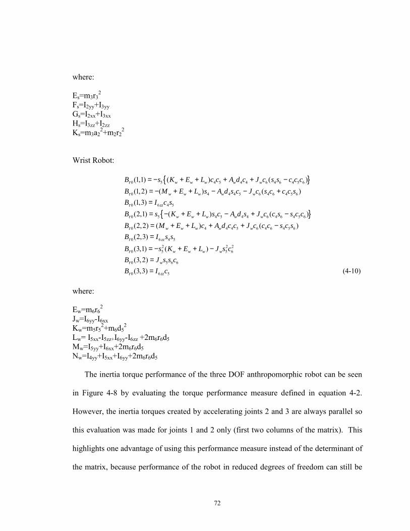
72

where: Es=m3r3

2

Fs=I2yy+I3yy Gs=I2xx+I3xx Hs=I3zz+I2zz Ks=m3a2

2+m2r22

Wrist Robot:

{ }

{ }

0 5 4 5 4 4 6 4 6 4 5 6

0 4 4 4 5 6 4 6 4 5 6

0 6 4 5

0 5 4 5 4 4 6 4 6 4 5 6

0 4 4 4 5

(1,1) ( ) ( )(1,2) ( ) ( )(1,3)(2,1) ( ) ( )(2,2) ( )

w w w w w

w w w w w

zz

w w w w w

w w w w

B s K E L c c A d c J c s s c c cB M E L s A d s c J c s c c c sB I c sB s K E L s c A d s J c c s s c cB M E L c A d c c J

τ

τ

τ

τ

τ

= − + + + + −= − + + − − +== − + + − + −= + + + + 6 4 6 4 5 6

0 6 4 5

2 2 20 5 5 6

0 5 6 6

0 6 5

( )(2,3)

(3,1) ( )(3,2)(3,3) (4-10)

w

zz

w w w w

w

zz

c c c s c sB I s sB s K E L J s cB J s s cB I c

τ

τ

τ

τ

−=

= − + + −==

where: Ew=m6r6

2

Jw=I6yy-I6xx Kw=m5r5

2+m6d52

Lw= I5xx-I5zz+I6yy-I6zz +2m6r6d5 Mw=I5yy+I6xx+2m6r6d5 Nw=I4yy+I5xx+I6yy+2m6r6d5

The inertia torque performance of the three DOF anthropomorphic robot can be seen

in Figure 4-8 by evaluating the torque performance measure defined in equation 4-2.

However, the inertia torques created by accelerating joints 2 and 3 are always parallel so

this evaluation was made for joints 1 and 2 only (first two columns of the matrix). This

highlights one advantage of using this performance measure instead of the determinant of

the matrix, because performance of the robot in reduced degrees of freedom can still be

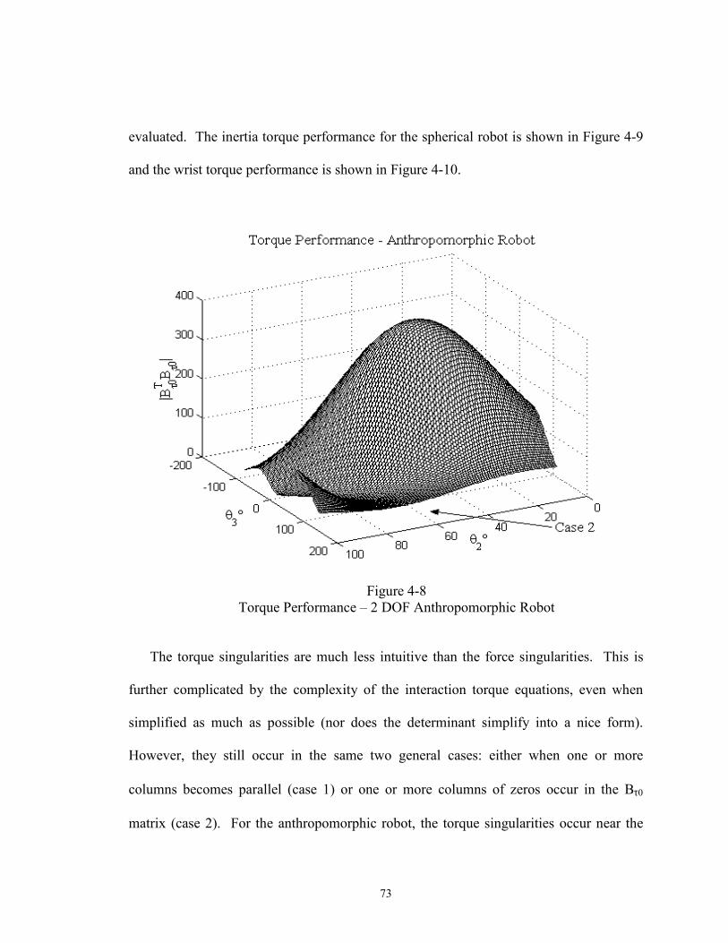
73

evaluated. The inertia torque performance for the spherical robot is shown in Figure 4-9

and the wrist torque performance is shown in Figure 4-10.

Figure 4-8

Torque Performance � 2 DOF Anthropomorphic Robot

The torque singularities are much less intuitive than the force singularities. This is

further complicated by the complexity of the interaction torque equations, even when

simplified as much as possible (nor does the determinant simplify into a nice form).

However, they still occur in the same two general cases: either when one or more

columns becomes parallel (case 1) or one or more columns of zeros occur in the Bτ0

matrix (case 2). For the anthropomorphic robot, the torque singularities occur near the

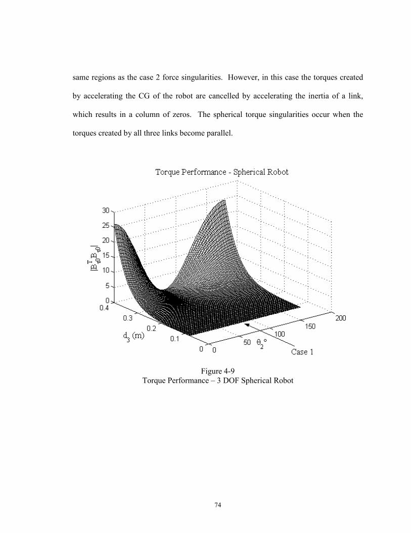
74

same regions as the case 2 force singularities. However, in this case the torques created

by accelerating the CG of the robot are cancelled by accelerating the inertia of a link,

which results in a column of zeros. The spherical torque singularities occur when the

torques created by all three links become parallel.

Figure 4-9

Torque Performance � 3 DOF Spherical Robot

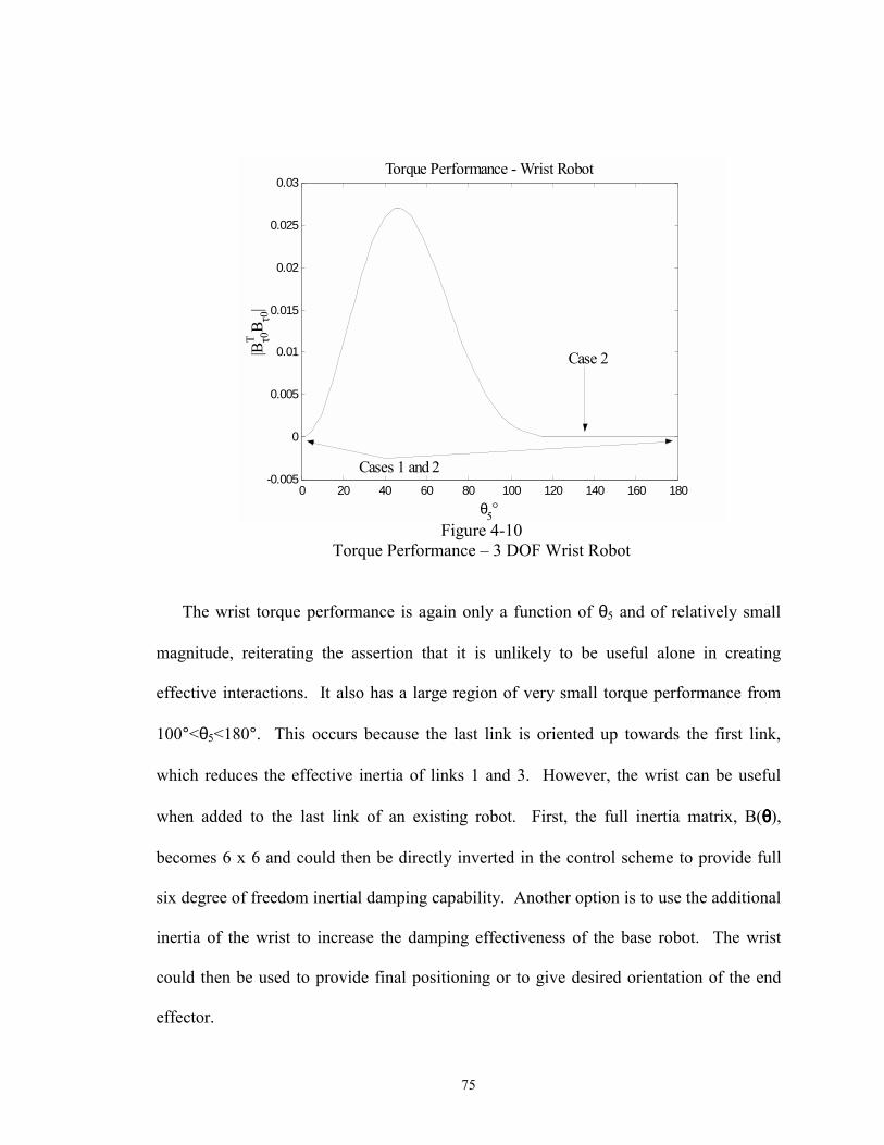
75

0 20 40 60 80 100 120 140 160 180-0.005

0

0.005

0.01

0.015

0.02

0.025

0.03Torque Performance - Wrist Robot

θ5°

|Bτ0T

B τ0|

Cases 1 and 2

Case 2

Figure 4-10

Torque Performance � 3 DOF Wrist Robot

The wrist torque performance is again only a function of θ5 and of relatively small

magnitude, reiterating the assertion that it is unlikely to be useful alone in creating

effective interactions. It also has a large region of very small torque performance from

100°<θ5<180°. This occurs because the last link is oriented up towards the first link,

which reduces the effective inertia of links 1 and 3. However, the wrist can be useful

when added to the last link of an existing robot. First, the full inertia matrix, B(θθθθ),

becomes 6 x 6 and could then be directly inverted in the control scheme to provide full

six degree of freedom inertial damping capability. Another option is to use the additional

inertia of the wrist to increase the damping effectiveness of the base robot. The wrist

could then be used to provide final positioning or to give desired orientation of the end

effector.

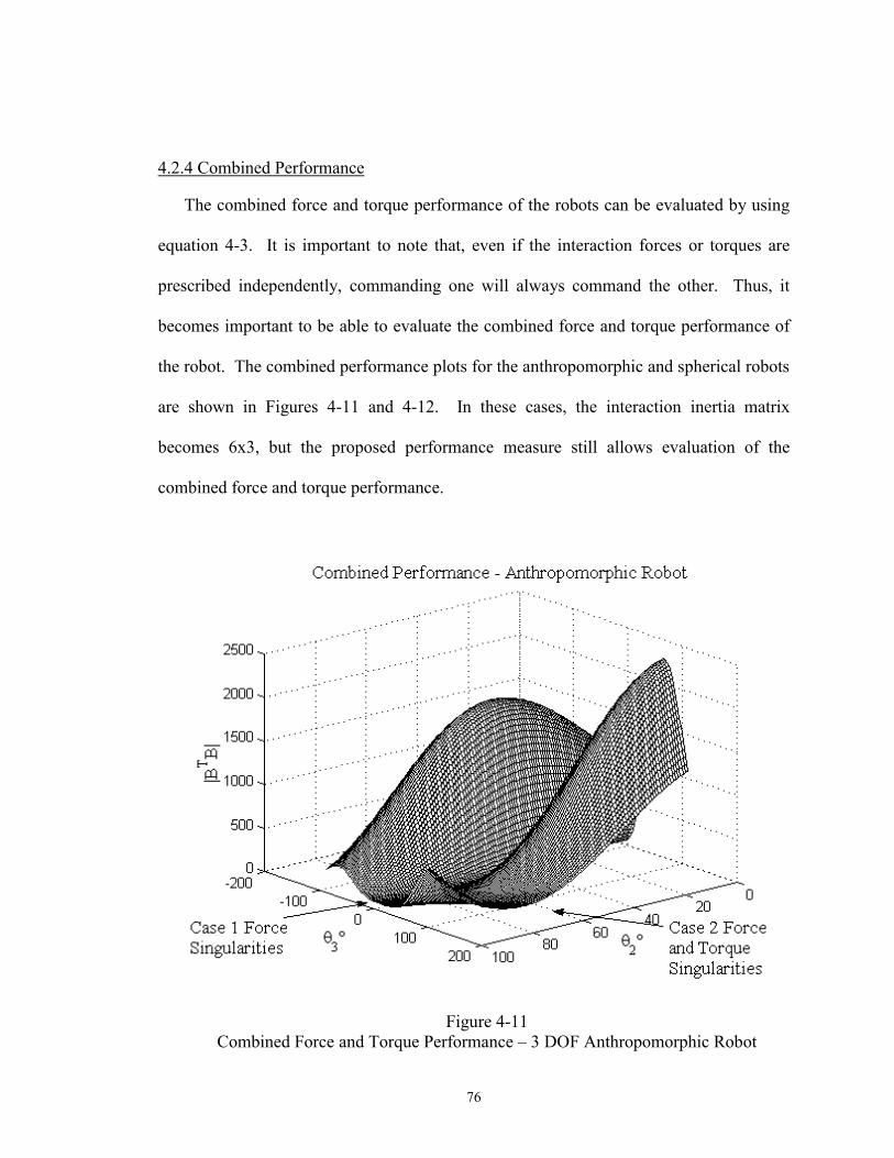
76

4.2.4 Combined Performance

The combined force and torque performance of the robots can be evaluated by using

equation 4-3. It is important to note that, even if the interaction forces or torques are

prescribed independently, commanding one will always command the other. Thus, it

becomes important to be able to evaluate the combined force and torque performance of

the robot. The combined performance plots for the anthropomorphic and spherical robots

are shown in Figures 4-11 and 4-12. In these cases, the interaction inertia matrix

becomes 6x3, but the proposed performance measure still allows evaluation of the

combined force and torque performance.

Figure 4-11

Combined Force and Torque Performance � 3 DOF Anthropomorphic Robot

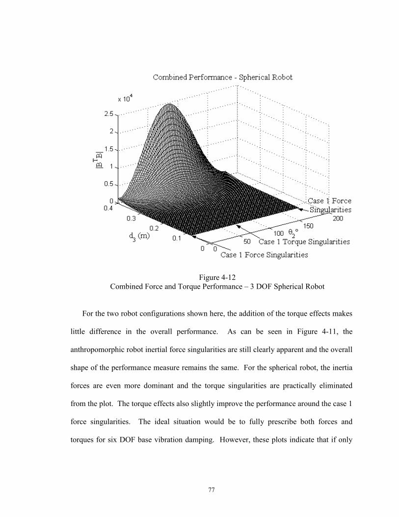
77

Figure 4-12

Combined Force and Torque Performance � 3 DOF Spherical Robot

For the two robot configurations shown here, the addition of the torque effects makes

little difference in the overall performance. As can be seen in Figure 4-11, the

anthropomorphic robot inertial force singularities are still clearly apparent and the overall

shape of the performance measure remains the same. For the spherical robot, the inertia

forces are even more dominant and the torque singularities are practically eliminated

from the plot. The torque effects also slightly improve the performance around the case 1

force singularities. The ideal situation would be to fully prescribe both forces and

torques for six DOF base vibration damping. However, these plots indicate that if only

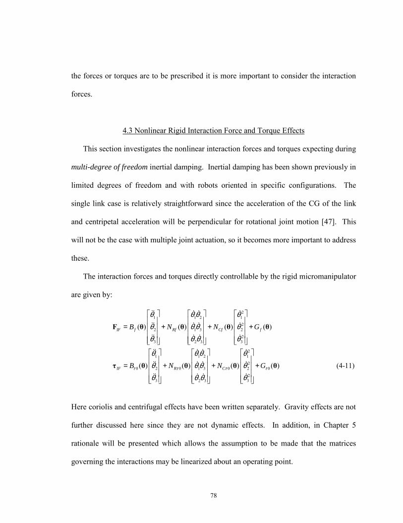
78

the forces or torques are to be prescribed it is more important to consider the interaction

forces.

4.3 Nonlinear Rigid Interaction Force and Torque Effects

This section investigates the nonlinear interaction forces and torques expecting during

multi-degree of freedom inertial damping. Inertial damping has been shown previously in

limited degrees of freedom and with robots oriented in specific configurations. The

single link case is relatively straightforward since the acceleration of the CG of the link

and centripetal acceleration will be perpendicular for rotational joint motion [47]. This

will not be the case with multiple joint actuation, so it becomes more important to address

these.

The interaction forces and torques directly controllable by the rigid micromanipulator

are given by:

21 1 2 1

22 1 3 2

23 32 3

21 1 2 1

20 2 0 1 3 0 2

23 32 3

( ) ( ) ( ) ( )

( ) ( ) ( )

IF f Rf Cf f

IF R C

B N N G

B N Nτ τ τ

θ θ θ θθ θ θ θθ θθ θ

θ θ θ θθ θ θ θθ θθ θ

= + + +

= + +

F θ θ θ θ

τ θ θ θ

&& & & &

&& & & &

&& && &

&& & & &

&& & & &

&& && &0 ( ) (4-11)Gτ

+

θ

Here coriolis and centrifugal effects have been written separately. Gravity effects are not

further discussed here since they are not dynamic effects. In addition, in Chapter 5

rationale will be presented which allows the assumption to be made that the matrices

governing the interactions may be linearized about an operating point.

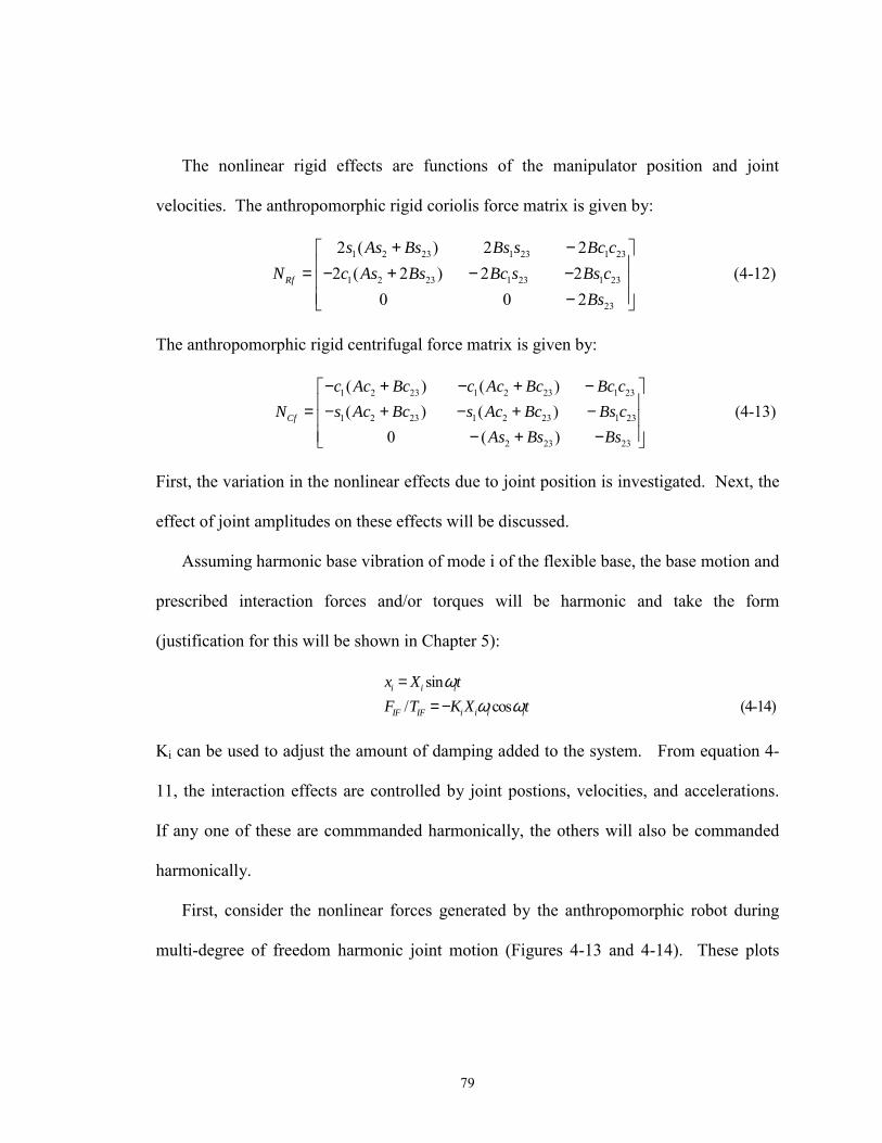
79

The nonlinear rigid effects are functions of the manipulator position and joint

velocities. The anthropomorphic rigid coriolis force matrix is given by:

1 2 23 1 23 1 23

1 2 23 1 23 1 23

23

2 ( ) 2 22 ( 2 ) 2 2 (4-12)

0 0 2 Rf

s As Bs Bs s Bc cN c As Bs Bc s Bs c

Bs

+ − = − + − − −

The anthropomorphic rigid centrifugal force matrix is given by:

1 2 23 1 2 23 1 23

1 2 23 1 2 23 1 23

2 23 23

( ) ( ) ( ) ( ) (4-13)

0 ( ) Cf

c Ac Bc c Ac Bc Bc cN s Ac Bc s Ac Bc Bs c

As Bs Bs

− + − + − = − + − + − − + −

First, the variation in the nonlinear effects due to joint position is investigated. Next, the

effect of joint amplitudes on these effects will be discussed.

Assuming harmonic base vibration of mode i of the flexible base, the base motion and

prescribed interaction forces and/or torques will be harmonic and take the form

(justification for this will be shown in Chapter 5):

sin/ cos (4-14)

i i i

IF IF i i i i

x X tF T K X t

ωω ω

==−

Ki can be used to adjust the amount of damping added to the system. From equation 4-

11, the interaction effects are controlled by joint postions, velocities, and accelerations.

If any one of these are commmanded harmonically, the others will also be commanded

harmonically.

First, consider the nonlinear forces generated by the anthropomorphic robot during

multi-degree of freedom harmonic joint motion (Figures 4-13 and 4-14). These plots

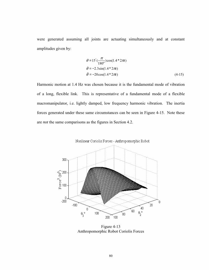
80

were generated assuming all joints are actuating simultaneously and at constant

amplitudes given by:

15 ( )cos(1.4 * 2 )180

2.3sin(1.4* 2 )20cos(1.4 * 2 ) (4-15)

t

tt

οπθ π

θ πθ π

°=

= −

= −

&

&&

Harmonic motion at 1.4 Hz was chosen because it is the fundamental mode of vibration

of a long, flexible link. This is representative of a fundamental mode of a flexible

macromanipulator, i.e. lightly damped, low frequency harmonic vibration. The inertia

forces generated under these same circumstances can be seen in Figure 4-15. Note these

are not the same comparisons as the figures in Section 4.2.

Figure 4-13

Anthropomorphic Robot Coriolis Forces

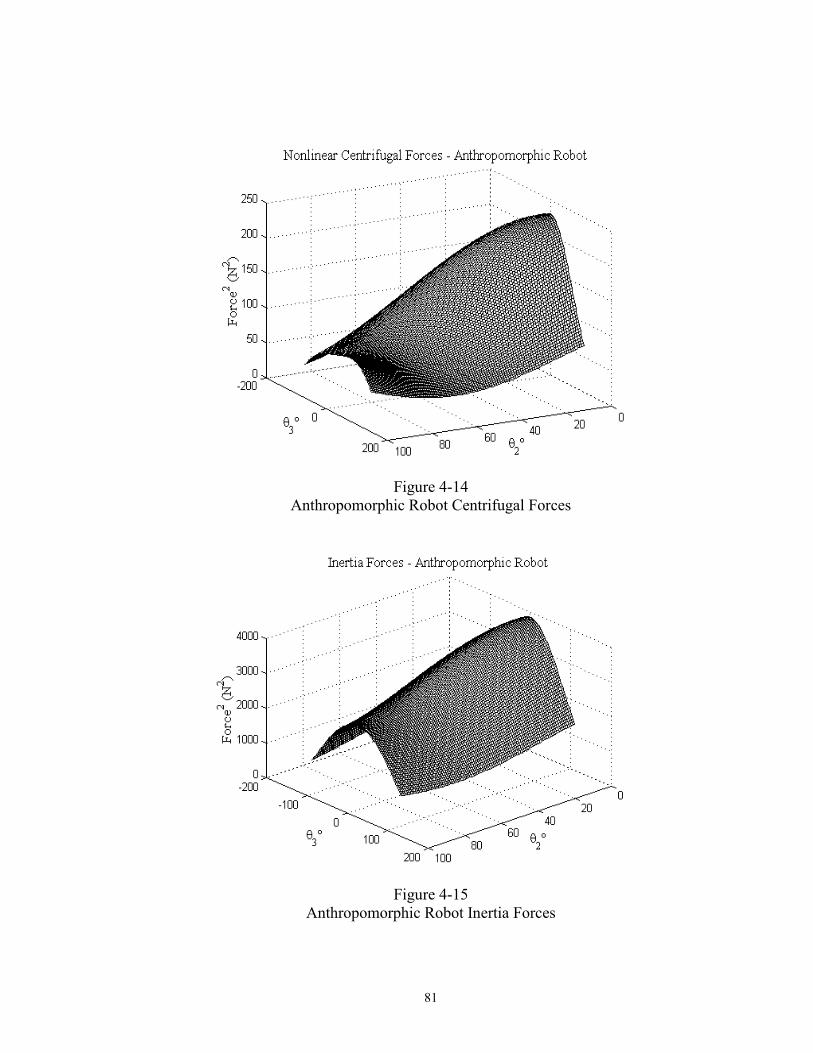
81

Figure 4-14

Anthropomorphic Robot Centrifugal Forces

Figure 4-15

Anthropomorphic Robot Inertia Forces

82

Although this initial analysis may be overconservative since it does not consider the

effect of decaying amplitudes or phasing, it does bring to light several important

considerations. First, the magnitude of the inertia forces is much larger than the

nonlinear forces. Second, coriolis forces are largest in near-singularity regions (case 2 in

Figure 4-5). Thus, the coriolis forces are not a great concern because operation in these

regions will be avoided by using the performance index. However, the centrifugal forces

are largest around the kinematic singularities (case 1 in Figure 4-5) and where the inertia

forces are largest, as shown in Figure 4-15. In fact, the centrifugal forces are maximum

at the singularity point θ2=0°, θ3=0°. Operation exactly at the singularity points will be

avoided, but operation around them may be required, especially if large inertia forces are

desired.

Since the anthropomorphic robot is always singular in three DOF inertia torque

performance, the spherical robot was chosen to study the nonlinear torque effects. The

spherical robot coriolis and centrifugal torque matrices are given by equations A-37 and

A-38 in Appendix A. Note the third link is prismatic, so r3 is a variable. Figures 4-16

and 4-17 show the variation in nonlinear torque performance throughout the joint

workspace and Figure 4-18 shows the inertia torques. These plots indicate that the

coriolis torques are greatest in joint configurations where the inertia torque effects are

largest. The centrifugal torques are largest in regions where the inertia torques are small,

indicating they will interfere less with the inertia torques. Again, the magnitude of the

inertia torques is greater than the nonlinear torques, but not to the same extent seen for

the anthropomorphic robot forces. Although these results are not presented here, the

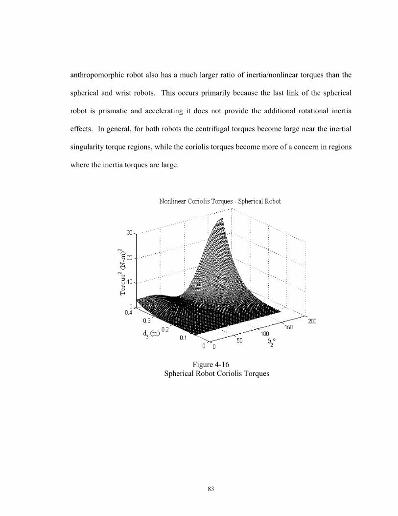
83

anthropomorphic robot also has a much larger ratio of inertia/nonlinear torques than the

spherical and wrist robots. This occurs primarily because the last link of the spherical

robot is prismatic and accelerating it does not provide the additional rotational inertia

effects. In general, for both robots the centrifugal torques become large near the inertial

singularity torque regions, while the coriolis torques become more of a concern in regions

where the inertia torques are large.

Figure 4-16

Spherical Robot Coriolis Torques

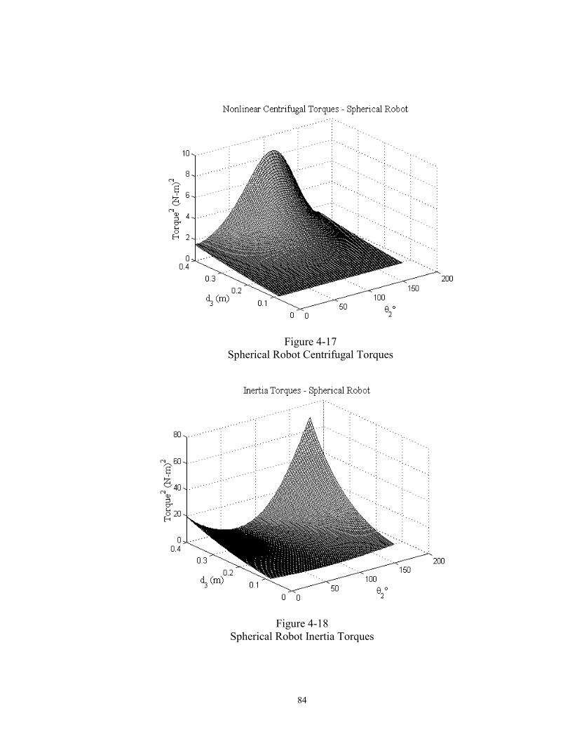
84

Figure 4-17

Spherical Robot Centrifugal Torques

Figure 4-18

Spherical Robot Inertia Torques

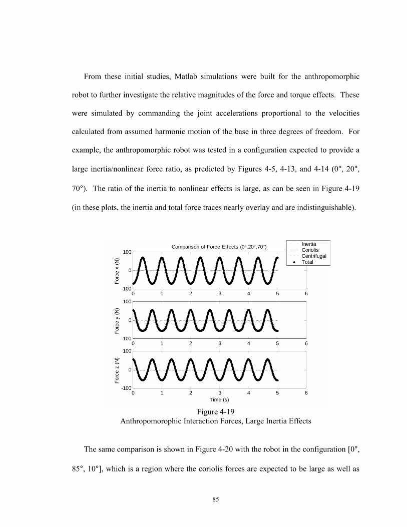
85

From these initial studies, Matlab simulations were built for the anthropomorphic

robot to further investigate the relative magnitudes of the force and torque effects. These

were simulated by commanding the joint accelerations proportional to the velocities

calculated from assumed harmonic motion of the base in three degrees of freedom. For

example, the anthropomorphic robot was tested in a configuration expected to provide a

large inertia/nonlinear force ratio, as predicted by Figures 4-5, 4-13, and 4-14 (0°, 20°,

70°). The ratio of the inertia to nonlinear effects is large, as can be seen in Figure 4-19

(in these plots, the inertia and total force traces nearly overlay and are indistinguishable).

0 1 2 3 4 5 6-100

0

100Comparison of Force Effects (0°,20°,70°)

Forc

e x

(N)

Inertia Coriolis CentrifugalTotal

0 1 2 3 4 5 6-100

0

100

Forc

e y

(N)

0 1 2 3 4 5 6-100

0

100

Time (s)

Forc

e z

(N)

Figure 4-19

Anthropomorophic Interaction Forces, Large Inertia Effects

The same comparison is shown in Figure 4-20 with the robot in the configuration [0°,

85°, 10°], which is a region where the coriolis forces are expected to be large as well as

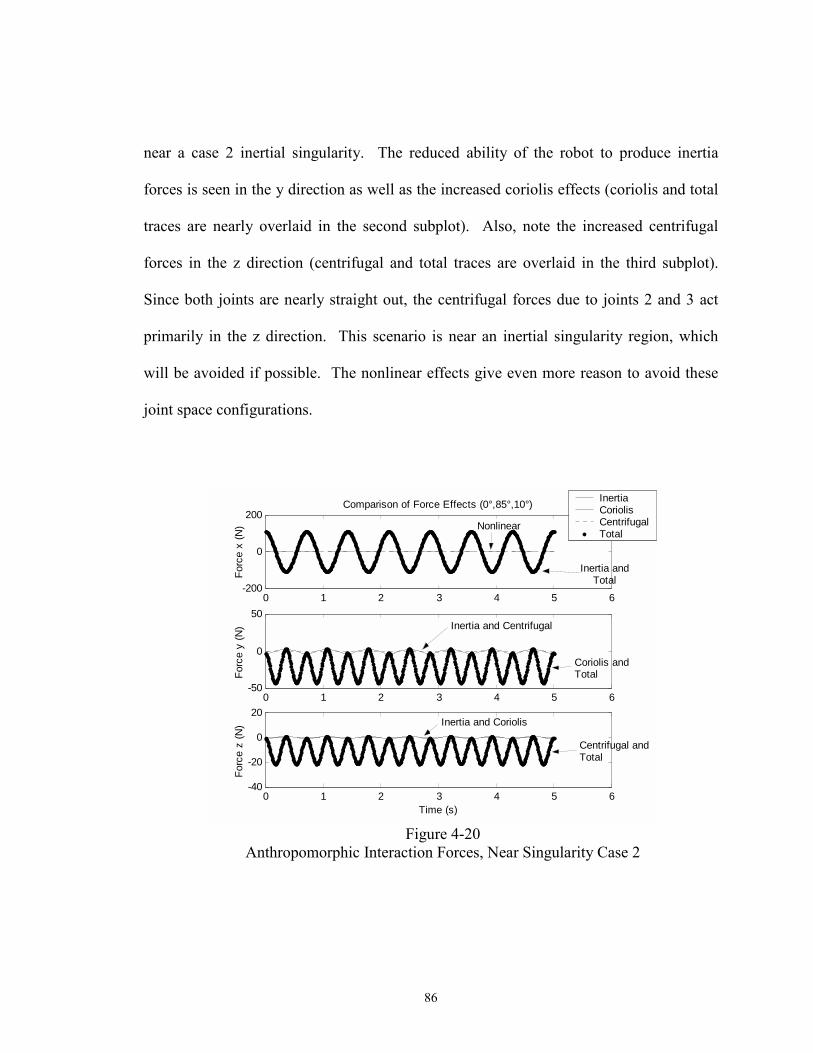
86

near a case 2 inertial singularity. The reduced ability of the robot to produce inertia

forces is seen in the y direction as well as the increased coriolis effects (coriolis and total

traces are nearly overlaid in the second subplot). Also, note the increased centrifugal

forces in the z direction (centrifugal and total traces are overlaid in the third subplot).

Since both joints are nearly straight out, the centrifugal forces due to joints 2 and 3 act

primarily in the z direction. This scenario is near an inertial singularity region, which

will be avoided if possible. The nonlinear effects give even more reason to avoid these

joint space configurations.

0 1 2 3 4 5 6-200

0

200Comparison of Force Effects (0°,85°,10°)

Forc

e x

(N)

Inertia Coriolis CentrifugalTotal

0 1 2 3 4 5 6-50

0

50

Forc

e y

(N)

0 1 2 3 4 5 6-40

-20

0

20

Time (s)

Forc

e z

(N)

Inertia and Total

Coriolis and Total

Centrifugal andTotal

Nonlinear

Inertia and Centrifugal

Inertia and Coriolis

Figure 4-20

Anthropomorphic Interaction Forces, Near Singularity Case 2

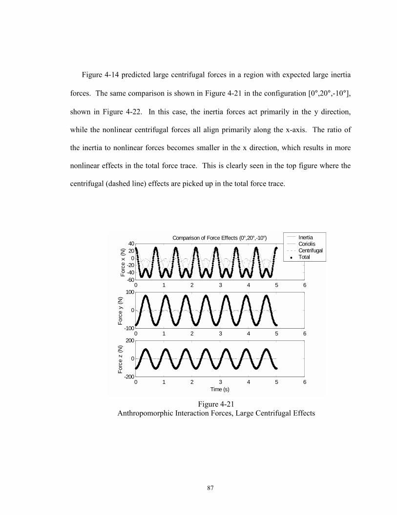
87

Figure 4-14 predicted large centrifugal forces in a region with expected large inertia

forces. The same comparison is shown in Figure 4-21 in the configuration [0°,20°,-10°],

shown in Figure 4-22. In this case, the inertia forces act primarily in the y direction,

while the nonlinear centrifugal forces all align primarily along the x-axis. The ratio of

the inertia to nonlinear forces becomes smaller in the x direction, which results in more

nonlinear effects in the total force trace. This is clearly seen in the top figure where the

centrifugal (dashed line) effects are picked up in the total force trace.

0 1 2 3 4 5 6-60-40-20

02040

Comparison of Force Effects (0°,20°,-10°)

Forc

e x

(N)

Inertia Coriolis CentrifugalTotal

0 1 2 3 4 5 6-100

0

100

Forc

e y

(N)

0 1 2 3 4 5 6-200

0

200

Time (s)

Forc

e z

(N)

Figure 4-21

Anthropomorphic Interaction Forces, Large Centrifugal Effects

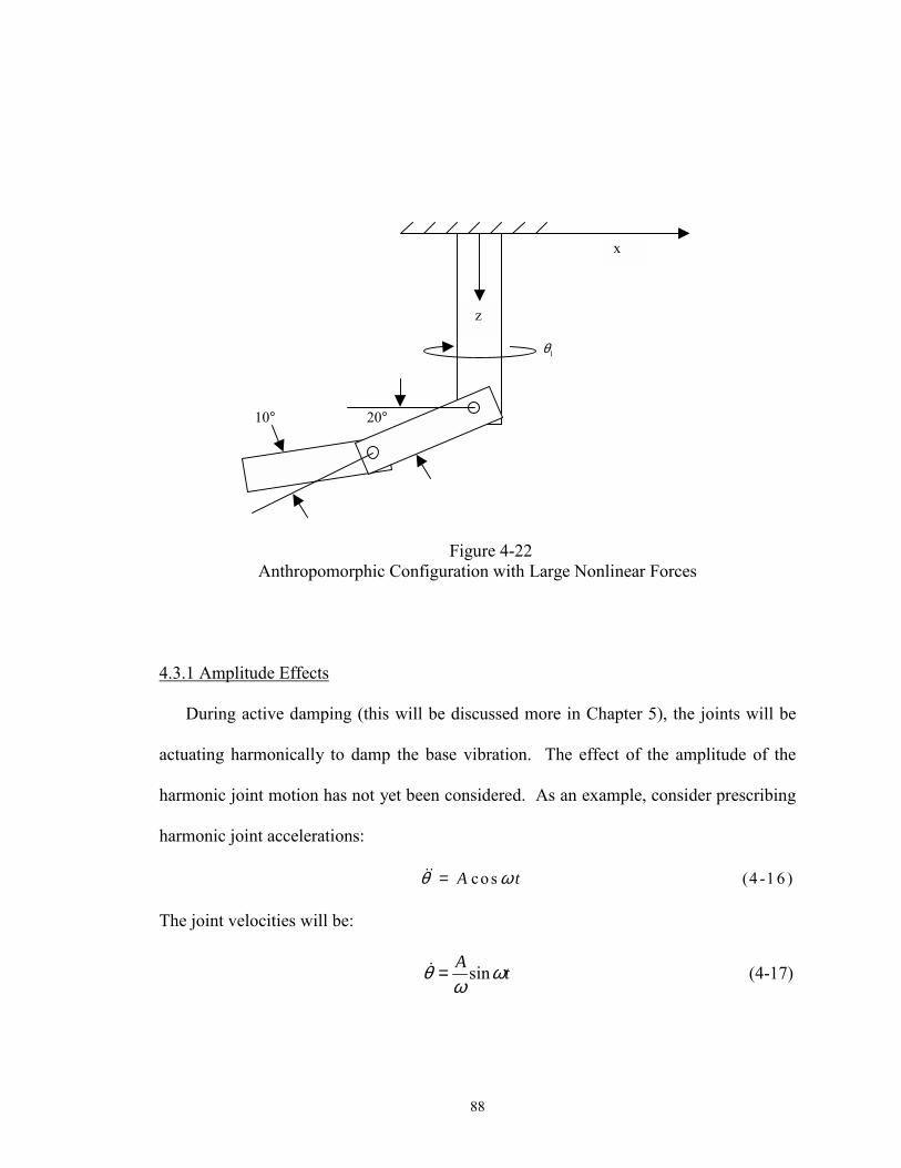
88

Figure 4-22

Anthropomorphic Configuration with Large Nonlinear Forces

4.3.1 Amplitude Effects

During active damping (this will be discussed more in Chapter 5), the joints will be

actuating harmonically to damp the base vibration. The effect of the amplitude of the

harmonic joint motion has not yet been considered. As an example, consider prescribing

harmonic joint accelerations:

co s (4 -1 6 )A tθ ω=&&

The joint velocities will be:

sin (4-17)A tθ ωω

=&

z

x

20°10°

1θ

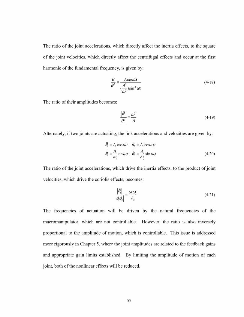
89

The ratio of the joint accelerations, which directly affect the inertia effects, to the square

of the joint velocities, which directly affect the centrifugal effects and occur at the first

harmonic of the fundamental frequency, is given by:

222

2

cos (4-18)( )sin

A tA t

θ ωθ ω

ω

=&&

&

The ratio of their amplitudes becomes:

2

2 (4-19)

Aθ ωθ

=&&

&

Alternately, if two joints are actuating, the link accelerations and velocities are given by:

1 1 1 2 2 2

1 21 1 2 2

1 2

cos cos

sin sin (4-20)

A t A tA At t

θ ω θ ω

θ ω θ ωω ω

= =

= =

&& &&

& &

The ratio of the joint accelerations, which drive the inertia effects, to the product of joint

velocities, which drive the coriolis effects, becomes:

1 1 2

21 2

(4-21)A

θ ωωθ θ

=&&

& &

The frequencies of actuation will be driven by the natural frequencies of the

macromanipulator, which are not controllable. However, the ratio is also inversely

proportional to the amplitude of motion, which is controllable. This issue is addressed

more rigorously in Chapter 5, where the joint amplitudes are related to the feedback gains

and appropriate gain limits established. By limiting the amplitude of motion of each

joint, both of the nonlinear effects will be reduced.

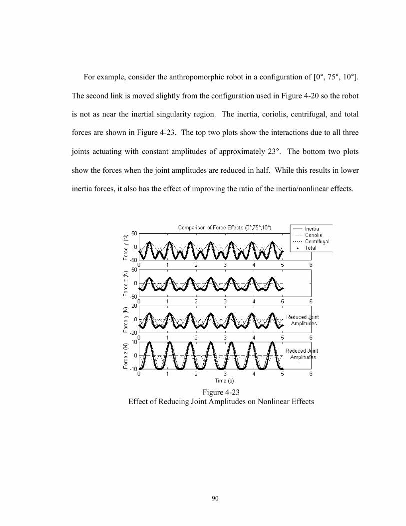
90

For example, consider the anthropomorphic robot in a configuration of [0°, 75°, 10°].

The second link is moved slightly from the configuration used in Figure 4-20 so the robot

is not as near the inertial singularity region. The inertia, coriolis, centrifugal, and total

forces are shown in Figure 4-23. The top two plots show the interactions due to all three

joints actuating with constant amplitudes of approximately 23°. The bottom two plots

show the forces when the joint amplitudes are reduced in half. While this results in lower

inertia forces, it also has the effect of improving the ratio of the inertia/nonlinear effects.

Figure 4-23

Effect of Reducing Joint Amplitudes on Nonlinear Effects

91

4.4 CG Method to Identify Critical Interaction Force Effects

This chapter concentrated on the interaction effects directly controllable by the rigid

robot, which are the inertia and nonlinear rigid effects. The method originally used to

develop the force equations is the Newton-Euler method described in Section 3.3.

However, a much more efficient method may be used to develop the interaction forces

directly controllable by the rigid robot. This made developing the six DOF

anthropomorphic/wrist force equations manageable and was the method used to derive

equations A-48 through A-50 in Appendix A.

The micromanipulator does not have a fixed point, so the interaction forces acting

between each link are found by summing the moments about the CG of each link.

Alternatively, the moments may be summed about the CG of the overall robot. The

position vectors to the CG of each robot are given in Appendix A. Let:

(4-22)CG CGJ=r θ&&

The interaction forces are given by:

( ) (4-23)IF CGd M Jdt

=F θ&

where M is the total mass of the rigid robot. The inertia and nonlinear rigid effects,

defined in Equation 4-1, are given by:

(4-24)f CG

f CG i

B MJ

N MJ θ

=

= &&

92

where Nf represents combined coriolis and centrifugal forces. If desired, the

macromanipulator inertia effects may be added by including the base direction cosine

matrix, which is defined and discussed in Book [8], Lew [34], and Senda [62].

1 1

1

(4-25)

z y

CG CGr z x CGr

y x

f f CGB A J

θ θθ θθ θ

− = + − + =

r r r

where rCGr is the position vector (from the base) to the CG of the rigid robot and θx, θy,

and θz are the small base rotations about the x, y, and z axis.

4.5 Conclusions

The interaction forces and torques will be used in the control scheme to add damping

to the flexible base. At this point, some general conclusions should be made about the

interaction effects, which will be used to develop the vibration controller and gain limits

discussed in Chapter 5.

1) The nonlinear and inertia effects are driven by two factors: the configuration of the

robot and joint accelerations and velocities. The inertia performance measure introduced

in equations 4-2 and 4-3 and plotted in Figures 4-5 through 4-12 can be used to choose

inverse kinematic solution(s) best suited for inertial damping. As an example, consider

the anthropomorphic robot in the two configurations shown in Figure 4-24. The left

configuration shows a very poor configuration for inertial damping (case 2 inertial

singularity), while the alternate inverse kinematics solution shown on the right will

provide much better inertia force performance.

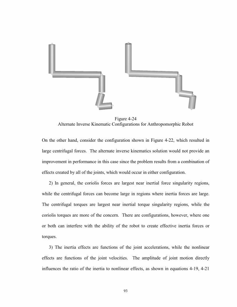
93

Figure 4-24 Alternate Inverse Kinematic Configurations for Anthropomorphic Robot

On the other hand, consider the configuration shown in Figure 4-22, which resulted in

large centrifugal forces. The alternate inverse kinematics solution would not provide an

improvement in performance in this case since the problem results from a combination of

effects created by all of the joints, which would occur in either configuration.

2) In general, the coriolis forces are largest near inertial force singularity regions,

while the centrifugal forces can become large in regions where inertia forces are large.

The centrifugal torques are largest near inertial torque singularity regions, while the

coriolis torques are more of the concern. There are configurations, however, where one

or both can interfere with the ability of the robot to create effective inertia forces or

torques.

3) The inertia effects are functions of the joint accelerations, while the nonlinear

effects are functions of the joint velocities. The amplitude of joint motion directly

influences the ratio of the inertia to nonlinear effects, as shown in equations 4-19, 4-21

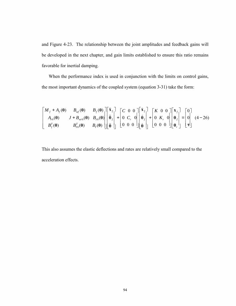
94

and Figure 4-23. The relationship between the joint amplitudes and feedback gains will

be developed in the next chapter, and gain limits established to ensure this ratio remains

favorable for inertial damping.

When the performance index is used in conjunction with the limits on control gains,

the most important dynamics of the coupled system (equation 3-31) take the form:

0 0 0

0

( ) ( ) ( ) 0 0 0 0 ( ) ( ) ( ) 0 0 0 0

0 0 0 0 0 0 ( ) ( ) ( )

f ff f wf f f

w f r f r fT T

rf

M A B B C KA J B B C KB B Bτ τ τ

τ τ

+ + + +

x xθ θ θ xθ θ θ θ θ θ

θθ θ θ θ θ

&& &

&& &

&& &

00 (4 26)

= − τ

This also assumes the elastic deflections and rates are relatively small compared to the

acceleration effects.

95

CHAPTER V

CONTROL SCHEME

5.1 Introduction

This chapter discusses the control scheme that will be used to provide position and

base vibration control of a flexible base manipulator. The goal of the control scheme is

to add to an existing position controller vibration damping capability. The rigid robot

will be commanded to provide the interaction forces and torques to damp the vibration.

An overview of the control scheme is shown in Figure 5-1. It is assumed the PID

position controller is designed separately for rigid robot control. The rigid robot model is

given by the third row of equation 3-27. The coupled rigid/flex dynamics are given by

the first two rows of equation 3-27, and the flexible manipulator is modeled by equation

3-19. The reason this form was chosen for the controller is discussed in Section 5.4.3.

Figure 5-1 Combined Position and Base Vibration Control Scheme

-

xf ττττ

- θθθθd θθθθa

PID

Position Control

F/ττττIF

Flexible Base Vibration Controller

xd

Inverse

Kinematics/ Damping

Performance Index Check

Rigid Robot

Coupled

Rigid/FlexDynamics

Flexible

Manipulator

96

First, the inverse kinematics/damping performance index check really consists of two

parts. The complete performance index will predict the overall ability of the control

scheme to be effective. This includes a comparison of the micromanipulator and

macromanipulator inertia properties as well as weighting matrices to include other

effects. The rigid robot performance measure that was introduced in equations 4-2 and 4-

3 will be used in the weighting matrix for the rigid robot and can be used to choose the

best inverse kinematics solutions for inertial damping.

Next, the vibration controller is introduced. One important goal of this section is to

establish a range of vibration control feedback gains to ensure vibration energy is

removed from the system. This involves establishing an upper limit that will limit the

joint amplitudes such that the interaction effects due to the joint accelerations are greater

than those due to the joint velocities, hence limiting the significance of the nonlinear

effects. In addition, a lower limit is established to ensure higher system modes will be

damped. Based on the results from Chapter 4, when the performance index is used along

with these control gains, the most important dynamics take the form of equation 4-26. In

order to add damping to the system, the joint accelerations will be commanded out of

phase with the flexible base velocity.

The control scheme takes advantage of the fact that the base vibrations are of

relatively high frequency compared to the rigid robot motion required to perform a task.

The separation of bandwidths, or time constants, between the position and vibration

control loops allows them to be considered separately. This is not addressed further here,

97

but more detail can be found in references [11], [33], and [35]. However, it is important

to check the validity of this assumption for the specific application.

It may be desirable in some cases to provide feedback proportional to the velocity and

position, akin to an ideal vibration absorber. This can give more flexibility in improving

system damping but requires additional measurements or manipulation of the measured

vibration data. However, the general form of the controller as well as guidelines for

choosing feedback gains will remain the same for either form.

Finally, the control performance of the linearized system will be discussed in the

single degree of freedom case. Root locus plots based on the linearized models verify

that, over a range of feedback gains, damping can be added to the flexible system. For

these studies, it has been assumed the rigid robot model takes the form of the third row in

equation 3-27. The hardware on which this control scheme was implemented was a

hydraulically operated robot. The actuator dynamics dominated the performance of the

experimental robot, so this effect is also discussed in Section 5.4.5.

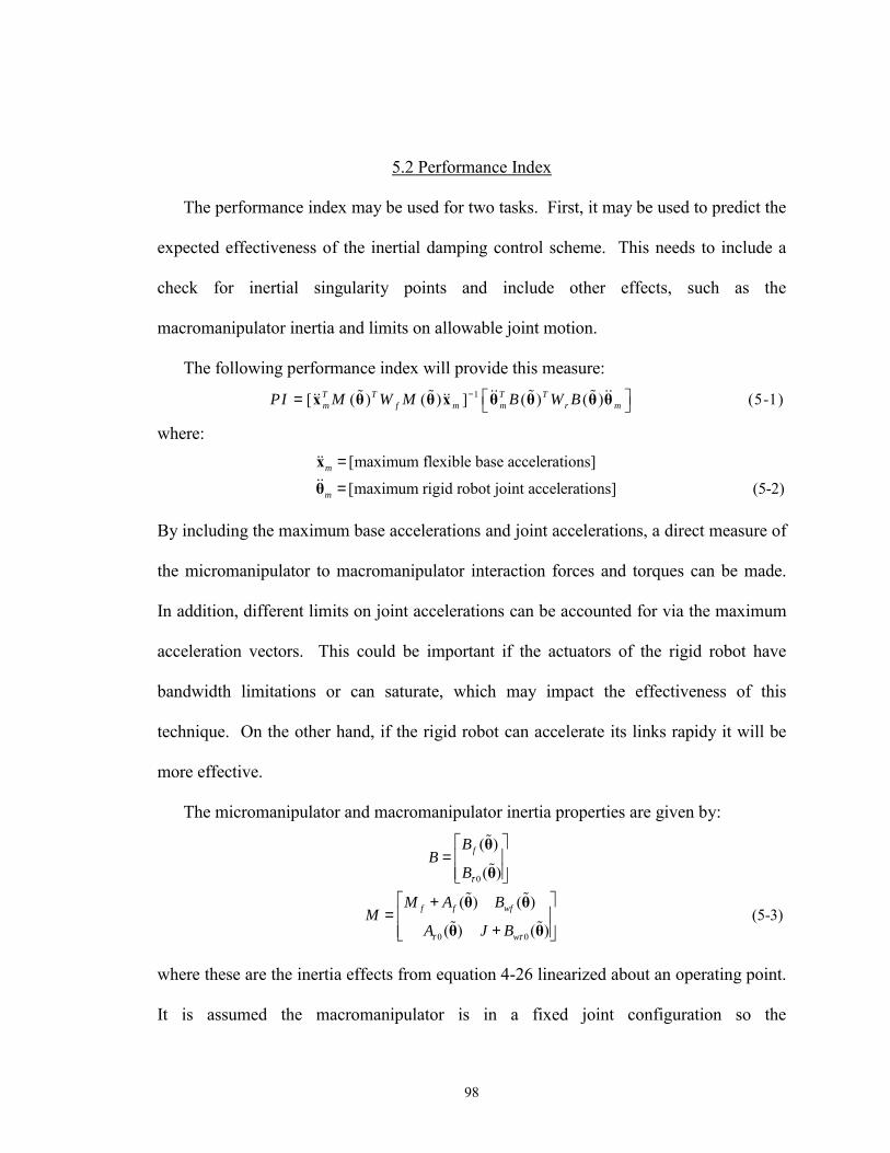
98

5.2 Performance Index

The performance index may be used for two tasks. First, it may be used to predict the

expected effectiveness of the inertial damping control scheme. This needs to include a

check for inertial singularity points and include other effects, such as the

macromanipulator inertia and limits on allowable joint motion.

The following performance index will provide this measure: 1[ ( ) ( ) ] ( ) ( ) (5-1)T T T T

m f m m r mPI M W M B W B− = x θ θ x θ θ θ θ% % && % % &&&& &&

where: [maximum flexible base accelerations]

[maximum rigid robot joint accelerations] (5-2)m

m

=

=

x

θ

&&

&&

By including the maximum base accelerations and joint accelerations, a direct measure of

the micromanipulator to macromanipulator interaction forces and torques can be made.

In addition, different limits on joint accelerations can be accounted for via the maximum

acceleration vectors. This could be important if the actuators of the rigid robot have

bandwidth limitations or can saturate, which may impact the effectiveness of this

technique. On the other hand, if the rigid robot can accelerate its links rapidy it will be

more effective.

The micromanipulator and macromanipulator inertia properties are given by:

0

0 0

( )

( )

( ) ( ) (5-3)

( ) ( )

f

f f wf

w

BB

B

M A BM

A J B

τ

τ τ

=

+=

+

θ

θ

θ θ

θ θ

%

%

% %

% %

where these are the inertia effects from equation 4-26 linearized about an operating point.

It is assumed the macromanipulator is in a fixed joint configuration so the

99

macromanipulator properties are assumed approximately constant, but in reality they will

vary with the configuration of the macromanipulator. Regardless, this performance

measure will predict the expected performance based on the inertia properties of the

macromanipulator in any configuration. The inertia matrices times the acceleration

vectors provide the forces and torques due to the flexible and rigid manipulators in each

direction. In the most general case, this results in two 6x1 vectors. The transpose of

these vectors times the vectors of the forces and torques results in a constant equal to the

sum of the square of the forces and torques. However, this measure alone does not

indicate whether the rigid robot has the ability to generate these interactions in multi-

degrees of freedom. Thus the weighting matrices need to be included.

The rigid robot weighting matrix is given by:

max

( ) ( ) N (5-4)

( ) ( )

T

r T

B BW

B B=

θ θ

θ θ

% %

% %

This was partially discussed in Chapter 4 along with its usefulness in determining joint

space configurations better suited for inertial damping. The only difference here is that it

is normalized, essentially assigning a penalty as the rigid robot moves away from its best

configuration. Another advantage of normalizing the performance measure is that the

units of the resulting BTB matrix do not matter.

Some authors have questioned the validity of eigenvalues and singular values for

systems with physical inconsistencies, such as robots with mixed prismatic and revolute

joints [20,60]. For example, the third link of the spherical robot is prismatic, so the Bf

matrix in equation 4-6 has units of mass for the third column while the other columns

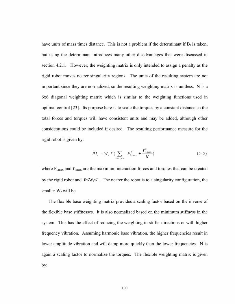
100

have units of mass times distance. This is not a problem if the determinant if Bf is taken,

but using the determinant introduces many other disadvantages that were discussed in

section 4.2.1. However, the weighting matrix is only intended to assign a penalty as the

rigid robot moves nearer singularity regions. The units of the resulting system are not

important since they are normalized, so the resulting weighting matrix is unitless. N is a

6x6 diagonal weighting matrix which is similar to the weighting functions used in

optimal control [23]. Its purpose here is to scale the torques by a constant distance so the

total forces and torques will have consistent units and may be added, although other

considerations could be included if desired. The resulting performance measure for the

rigid robot is given by:

2,m ax2

,m ax, ,

* ( ) (5-5)ir r i

i x y zPI W F

Nτ

=

= +∑

where Fi,max and τi,max are the maximum interaction forces and torques that can be created

by the rigid robot and 0≤Wr≤1. The nearer the robot is to a singularity configuration, the

smaller Wr will be.

The flexible base weighting matrix provides a scaling factor based on the inverse of

the flexible base stiffnesses. It is also normalized based on the minimum stiffness in the

system. This has the effect of reducing the weighting in stiffer directions or with higher

frequency vibration. Assuming harmonic base vibration, the higher frequencies result in

lower amplitude vibration and will damp more quickly than the lower frequencies. N is

again a scaling factor to normalize the torques. The flexible weighting matrix is given

by:

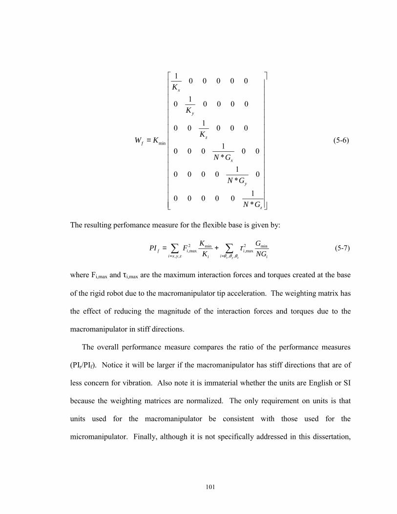
101

min

1 0 0 0 0 0

1 0 0 0 0 0

1 0 0 0 0 0 (5-6)

1 0 0 0 0 0*

1 0 0 0 0 0*

1 0 0 0 0 0*

x

y

zf

x

y

z

K

K

KW K

N G

N G

N G

=

The resulting perfomance measure for the flexible base is given by:

2 2min min,max ,max

, , , ,

(5-7)x y z

f i ii x y z ii i

K GPI FK NGθ θ θ

τ= =

= +∑ ∑

where Fi,max and τi,max are the maximum interaction forces and torques created at the base

of the rigid robot due to the macromanipulator tip acceleration. The weighting matrix has

the effect of reducing the magnitude of the interaction forces and torques due to the

macromanipulator in stiff directions.

The overall performance measure compares the ratio of the performance measures

(PIr/PIf). Notice it will be larger if the macromanipulator has stiff directions that are of

less concern for vibration. Also note it is immaterial whether the units are English or SI

because the weighting matrices are normalized. The only requirement on units is that

units used for the macromanipulator be consistent with those used for the

micromanipulator. Finally, although it is not specifically addressed in this dissertation,

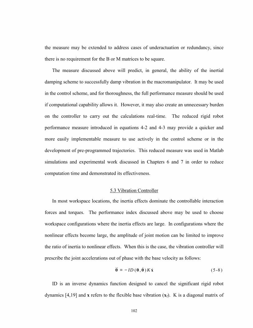
102

the measure may be extended to address cases of underactuation or redundancy, since

there is no requirement for the B or M matrices to be square.

The measure discussed above will predict, in general, the ability of the inertial

damping scheme to successfully damp vibration in the macromanipulator. It may be used

in the control scheme, and for thoroughness, the full performance measure should be used

if computational capability allows it. However, it may also create an unnecessary burden

on the controller to carry out the calculations real-time. The reduced rigid robot

performance measure introduced in equations 4-2 and 4-3 may provide a quicker and

more easily implementable measure to use actively in the control scheme or in the

development of pre-programmed trajectories. This reduced measure was used in Matlab

simulations and experimental work discussed in Chapters 6 and 7 in order to reduce

computation time and demonstrated its effectiveness.

5.3 Vibration Controller

In most workspace locations, the inertia effects dominate the controllable interaction

forces and torques. The performance index discussed above may be used to choose

workspace configurations where the inertia effects are large. In configurations where the

nonlinear effects become large, the amplitude of joint motion can be limited to improve

the ratio of inertia to nonlinear effects. When this is the case, the vibration controller will

prescribe the joint accelerations out of phase with the base velocity as follows:

( , ) (5 -8 )ID K= −θ θ θ x&& & &

ID is an inverse dynamics function designed to cancel the significant rigid robot

dynamics [4,19] and x refers to the flexible base vibration (xf). K is a diagonal matrix of

103

gains Ki, where Ki is the gain for the ith vibrational degree of freedom. With the limits on

gains that will be developed in the next section, the inertia effects are expected to be most

significant. Thus the prescribed joint accelerations will be:

1( ) (5-9)B K−= −θ θ x&& &

However, the joint torques will need to be commanded so the final vibration controller

takes the form:

1( ) ( ) ( ) ( 5 -1 0 )B B Kτ−= −τ θ θ x&

Bτ(θ) is as defined in equation 3-27 and

0

( ) (5-11)

( )fB

BBτ

=

θθ

It is assumed the rigid robot joint positions, θθθθ, are measured and available for use in

the control scheme. There should be a minimum value established for the determinant of

the inertia matrix to prevent it from being inverted when the robot is passing through a

singularity configuration. Although these regions will be avoided for point-to-point

motion and fixed configuration operation, it may be necessary to pass through the

singularity regions. In this case, it will become necessary to limit the commanded output

from the controller.

5.3.1 Vibration Control Gains

The goal of this section is to establish a range of vibration control feedback gains to

ensure vibration energy is removed from the system. The upper limit is developed in

order to limit the joint amplitudes such that the interaction effects due to joint

accelerations (inertia effects) are greater than those due to the joint velocities, hence

104

limiting the significance of the nonlinear effects. In addition, a lower limit is established

to ensure higher system modes will be damped.

5.3.1.1 Upper Limit

In order to establish an upper limit on the feedback gains, first assume harmonic base

vibration of mode i. As discussed in Chapter 4, assuming harmonic motion of the rigid

robot, the inertia effects will be functions of the joint accelerations and, with the proper

limit on the amplitude of joint motion, will be greater than the nonlinear effects. Thus,

the vibration controller will prescribe the joint accelerations out of phase with the base

velocity in order to add damping to the flexible base.

The prescribed joint accelerations, velocities, and positions for the jth joint will be

approximately harmonic and take the form:

1

1

1

ii

sin

( ) cos

( ) sin

( ) = cos t (5-12)

i i i

j i i i i

j i i i

i ij

x X t

B K X t

B K X t

B K X

ωω ω

ω

ωω

−

−

−

=

= −

= −

θ θ

θ θ

θθ

&& %

& %

%

Here is it assumed the inertia matrix, B(θθθθ), can be linearized and is approximately

constant about an operating point. The feedback gains will be selected to ensure this is a

reasonable assumption and will be discussed in more detail later.

The maximum amplitude of the prescribed joint motion will occur during the first few

cycles of vibration damping and for each joint can be written as:

1( ) (5-13)i ij

i

K B X Aθω

−

= ≡θ%

105

where A is defined as the amplitude of motion. It is clear that an upper limit on the

feedback gains is necessary, if for no other reason than to ensure the joint motion remains

inside the allowable workspace or to prevent actuator saturation. Another consideration

is the ratio of the inertia effects (functions of the joint accelerations) to the nonlinear

effects (functions of products of the joint velocities). This was discussed extensively in

section 4.3.1, and Figure 4-23 showed that the ratio of inertia effects to nonlinear effects

can be improved by reducing the amplitude of joint motion. Here, the centrifugal effects

are considered, so these become functions of the square of the joint velocities:

1i

2 2 22

( ) ( )= (5-14)( )

j i i i

i ii ij

B K X BK XB K X

θ ω ωθ

−

−

−=−

θ θθ

&& % %

%&

Solving equation 5-13 for Ki and substituting into equation 5-14 yields:

2

2 22

1 (5-15)j i

ij

AA A

θ ωωθ

= =&&

&

Likewise, the ratio of inertia to coriolis effects takes the form:

(5-16)j i

j ji j Aθ ω

ωθθ=

&&

& &

where ωi and ωj are two different frequencies of base vibration.

Notice by relating the feedback gains to the amplitude of joint motion, the ratios

become inversely proportional to the amplitude of motion, A. Thus, A can be limited to

ensure the joint acceleration effects remain larger than joint velocity effects. One upper

limit is A<1 radian, although there may be more restrictive limits due to other

considerations. The gains should be limited such that:

106

min min

max

( ) (5-17)ii

i

BK AX

ω< θ%

The true multi degree-of freedom case is more complex, of course. In addition, the

selection of A and Bmin will be specific to the macro/micromanipulator. The inertia and

force effects also vary throughout the workspace, as discussed in Chapter 4. However,

the above limit will help reduce the significance of the nonlinear effects, even when in

workspace locations where they can become large. Also, note this ratio improves with

decreasing amplitude, which increases the effectiveness of the scheme as the vibration is

damped.

This limit also helps validate the assumption that the inertia matrix B can be

linearized about an operating point. Consider the sensitivity of the inertia matrix to

changes in the joint positions. In order to keep this argument general, these matrices

consist of terms involving sines, cosines, and combinations of sines and cosines. This

general argument is intended to provide an example representative of all of the rigid robot

effects (inertia, nonlinear, and gravity matrices). In order to determine the error

introduced by evaluating B at an operating point, expand B in a Taylor series [6]:

( )( ) ( ) (5-18)ii

BB B θθ

=

∂+ ∆ ∂ θ θ

θθ θ%

%$

where ∆θi is harmonic and given by the last equation in 5-12. The inertia matrix B as

well as its first partial derivatives are bounded and continuous. The limits on joint

amplitudes will ensure the variation term remains small. Also, note this assumption

becomes more valid as energy is removed from the system because the joint amplitudes

are reduced. This, in general, is applicable to all of the rigid robot effects.

107

5.3.1.2 Lower Limit

A lower limit also needs to be established to ensure higher flexible system modes, if

excited, will be damped. The nonlinear effects will still be commanded along with the

damping effects. Here a worst-case scenario is considered where the nonlinear effects

excite a mode of the flexible system. The goal here is ensure net energy removal from

the system.

Assume an initial impulse force δ (N) applied over a finite amount of time T excites a

fundamental mode of the flexible system. The rate of change of energy added to the

flexible base is:

i = X cos (5-19)i i

dW xdt

N mts

δ

δ ω ω

=

−

&

where the base motion is given by the first equation in 5-12. The energy added to the

flexible base is given by:

0

i 0

i

cos

= X sin

= X sin (N-m) (5-20)

T

i i i

Ti

i

W X tdt

t

T

δω ω

δ ωδ ω

∆ = ∫

The rate of change of energy dissipated by the damping controller is [59]:

2 (5-21)idW K xdt

= − &

Over one cycle of vibration, the net energy dissipated by the vibration controller is:

108

22 2 2

0

2

2 2

0

2

cos

sin 2 = 2 4

= (5-22)

i

i

i i i i

ii i i

i

i i i

W K X tdt

ttK X

K X

πω

πω

ω ω

ωωω

ω π

∆ = −

− +

−

∫

This holds regardless of whether velocity feedback alone is used or if velocity and

position feedback are used. This is the energy removed over each cycle of vibration, so

as long as the disturbance is applied over a finite period, the vibration controller will

remove energy from the system.

Based on linearizing the system and assuming harmonic motion over each cycle of

vibration, the nonlinear centrifugal forces take the form (the same form applies to the

nonlinear torques):

2

2 2 2 2

2 2 2

( )

( ) ( ) sin

( ) ( )(1 cos 2 ) (5-23)

2

Ni f j

Ni f i i i

f i iNi i

F N

F N B K X t

N B K XF t

ω

ω

−

−

=

=

= −

θ θ

θ θ

θ θ

% &

% %

% %

where Nf represents NCf or NCτ0 given in equation 4-11 for forces and torques,

respectively and (sinωit)2 was replaced by an equivalent trigonometric identity. Define Y

as the amplitude of the nonlinear forces, or:

2 2 2( ) ( )( ) (5-24)

2f i iN B K X

Y−

≡θ θ

θ% %

%

Y may be assumed approximately constant since Nf and B may be assumed

approximately constant about an operating point, as discussed in section 5.3.1.1. The

109

nonlinear force may be split into two terms, Y and �Ycos2ωit. The rate of change of

energy added to the system due to the first term is given by:

( ) cos (5-25)i i idW Y X tdt

ω ω= θ%

Regardless of the mode or number of modes excited, if Y is approximately constant the

net work over each cycle of vibration will be small since:

2

0( ) cos 0 (5-26)i

in i i iW Y X tdtπω ω ω∆ = ≈∫θ%

and the vibration controller will remove any energy added.

The effect of the second term is more interesting. Define the first harmonic of the

fundamental frequency as:

2 (5-27)i iω ω=

Consider the flexible base as a damped system responding to a harmonic forcing, or

2 2 2 ( )cos (5-28)iMx Cx Kx Y tω+ + = − θ%&& &

where M, C, and K are inertia, damping, and stiffness properties of the

macromanipulator and the natural frequency and damping ratio of the flexible base mode

are given by ωn and ζ, respectively. Assume the resulting vibration will take the form:

2 2 cos( ) (5-29)ix X tω φ= −

where X2 is the amplitude of the vibration and φ the resulting phase shift.

110

Substituting 5-29 into 5-28 and solving for the resulting amplitude and phase shift yields:

2

2 2 2 2

1 ( ) (2 ) (5-30)n i i n

YXL

LM

ω ω ζω ω

−=

= − +

2

2 2n

tan

2 = (5-31)

i

i

n i

i

CK M

ωφω

ζω ωω ω

=−

−

The rate of change of energy into the system and net energy added over one cycle of

vibration becomes:

2

2 22

2 20 0

2

co s * sin ( )

cos cos sin sin cos

sin (5 -32)

i i

i i i

in i i i i i

dW YX t td t

W YX t td t YX td t

YX

π πω ω

ω ω ω φ

ω φ ω ω ω φ ω

π φ

= −

∆ = −

= −∫ ∫

Substituting 5-30 into 5-32 gives the net energy added to the system over one cycle of

vibration:

2 sin (5-33)inYW

Lφπ∆ =

The net energy dissipated by the vibration controller over one cycle of vibration is:

222 2 (5-34)i i

out i iK YW K X

Lω πω π −∆ = − =

In order to ensure energy dissipation, the goal is to choose Ki such that ∆Wout+∆Win<0.

This relationship becomes:

s in 0 (5 -3 5 )i iK Lω φ− + <

The worst-case scenario occurs when the nonlinear harmonics occur exactly at a natural

frequency of the system, or when and sin 1i nω ω φ= = in which case:

111

2

i

1 (2 )

2 = (5-36)M

i n

n

LM

ζωω

ζωω

=

±

Thus the lower limit on the control gain to ensure net energy dissipation becomes:

2 (5-37)niK

Mζω> ±

Consider the meaning of this lower limit. As long as the vibration control gains are

selected such that the vibration controller adds no more energy to higher system modes

than that which can be dissipated by the natural damping in the system, overall vibration

energy will be removed from the system. However, this lower limit analysis only

considers the higher system modes. In order to prevent excitation of them along with

other negative consequences of using negative feedback gains, the lower limit is

realistically chosen as zero. Using the upper limit established previously, limiting the

gains to the range:

,m in m in

,m a x

( )0 A (5 -3 8 )i

ii

BK

Xω

< <θ%

will ensure effects due to joint accelerations are larger than those due to joint velocities,

hence the inertia effects will also be larger. It also ensures there is enough damping

available to successfully remove vibration energy from higher modes of vibration (if a

concern) if they are excited.

5.4 Controller Performance

This section investigates the control performance of the linearized system, for both

ideal robot models as well as a hydraulically operated robot. Using the linearized model

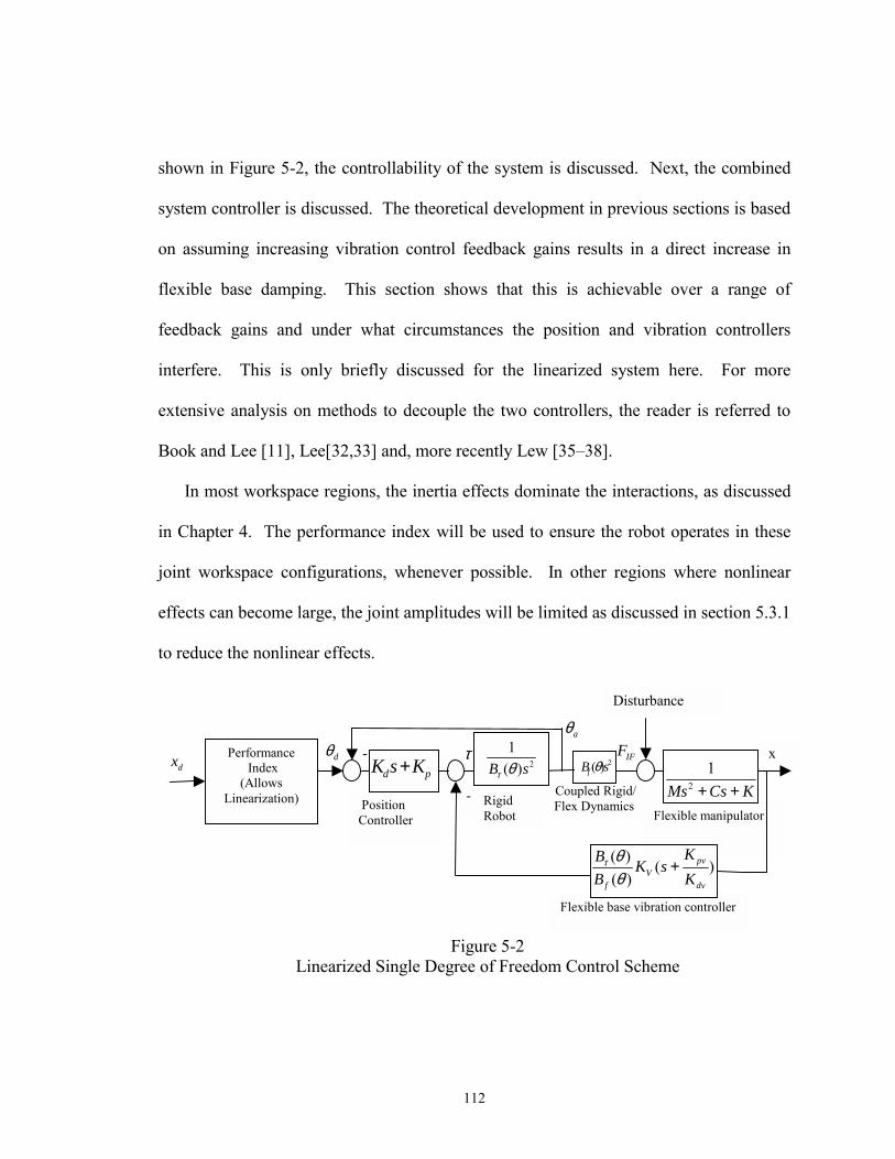
112

shown in Figure 5-2, the controllability of the system is discussed. Next, the combined

system controller is discussed. The theoretical development in previous sections is based

on assuming increasing vibration control feedback gains results in a direct increase in

flexible base damping. This section shows that this is achievable over a range of

feedback gains and under what circumstances the position and vibration controllers

interfere. This is only briefly discussed for the linearized system here. For more

extensive analysis on methods to decouple the two controllers, the reader is referred to

Book and Lee [11], Lee[32,33] and, more recently Lew [35�38].

In most workspace regions, the inertia effects dominate the interactions, as discussed

in Chapter 4. The performance index will be used to ensure the robot operates in these

joint workspace configurations, whenever possible. In other regions where nonlinear

effects can become large, the joint amplitudes will be limited as discussed in section 5.3.1

to reduce the nonlinear effects.

Figure 5-2 Linearized Single Degree of Freedom Control Scheme

Flexible base vibration controller

Coupled Rigid/ Flex Dynamics

Flexible manipulator

x -

- Position Controller

Disturbance

Performance Index

(Allows Linearization)

Rigid Robot

2

1( )B sτ θdx dθ

d pK s K+τ

aθ

2( )fB sθIFF

2

1Ms Cs K+ +

( ) ( )( )

pvV

f dv

KB K sB Kτ θθ

+

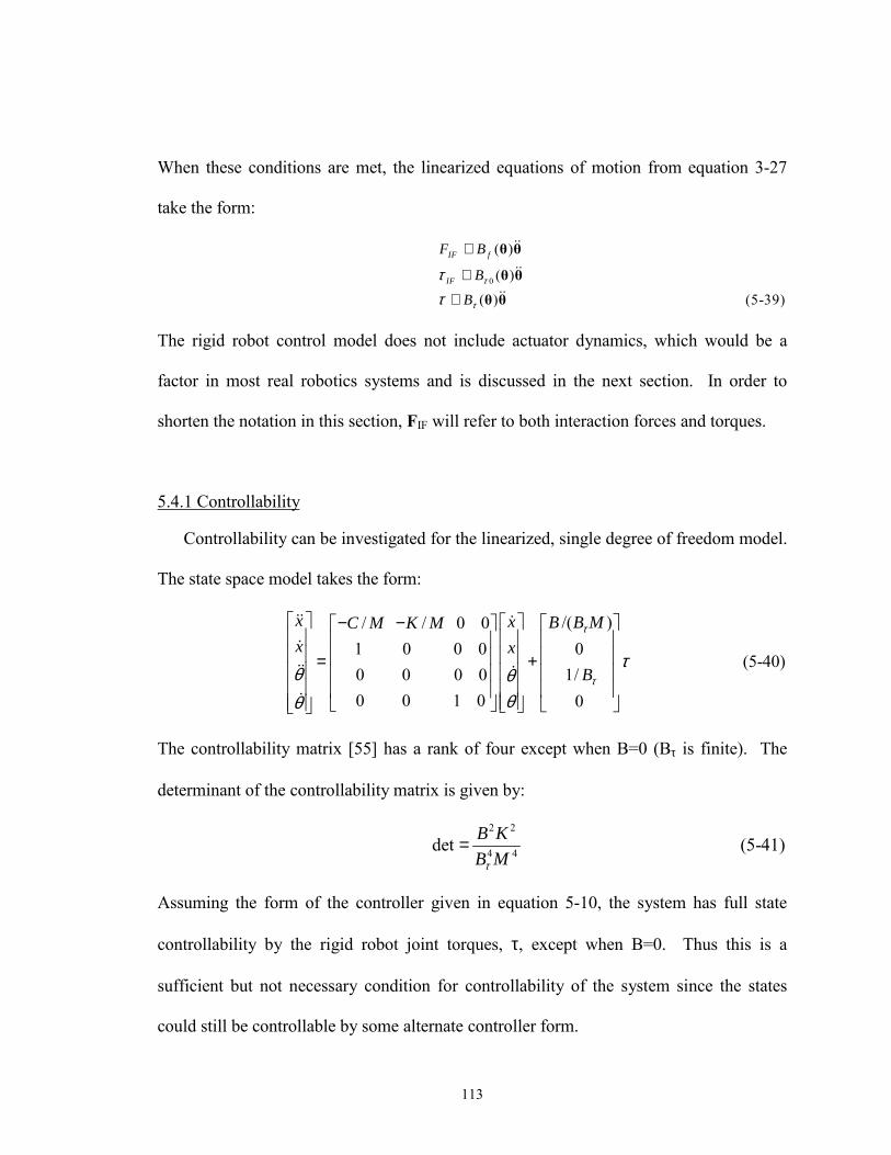
113

When these conditions are met, the linearized equations of motion from equation 3-27

take the form:

0

( )

( )

( ) (5-39)

IF f

IF

F B

B

Bτ

τ

ττ

≅

≅

≅

θ θ

θ θ

θ θ

&&

&&

&&

The rigid robot control model does not include actuator dynamics, which would be a

factor in most real robotics systems and is discussed in the next section. In order to

shorten the notation in this section, FIF will refer to both interaction forces and torques.

5.4.1 Controllability

Controllability can be investigated for the linearized, single degree of freedom model.

The state space model takes the form:

/( )/ / 0 0 1 0 0 0 0

0 0 0 0 1/ 0 0 1 0 0

x x B B MC M K Mx x

B

τ

τ

τθ θ

θθ

− − = +

&& &

&

&& &

&

(5-40)

The controllability matrix [55] has a rank of four except when B=0 (Bτ is finite). The

determinant of the controllability matrix is given by:

2 2

4 4det (5-41)B KB Mτ

=

Assuming the form of the controller given in equation 5-10, the system has full state

controllability by the rigid robot joint torques, τ, except when B=0. Thus this is a

sufficient but not necessary condition for controllability of the system since the states

could still be controllable by some alternate controller form.

114

For the multi-degree of freedom case, this corresponds to an inertial singularity point

discussed in Chapter 4. In these configurations, the rank of the controllability matrix

reduces to two and, assuming the use of the controller in equation 5-10, the rigid robot

inertia matrix is not invertible. Another problem situation occurs when the ratio of

macromanipulator stiffness to inertia (K/M) becomes very small, which indicates an

extremely flexible base or large macromanipulator. This would also present a problem

since there will be no coupling between the rigid robot interactions and the mode of

vibration. Note the performance index described in section 5.2 would also predict

impacted performance in all of these scenarios.

5.4.2 Ideal Rigid Robot Model Control Performance

The general case of position and velocity feedback is investigated here (gain limits

developed in Section 5.3.1 are applicable for either case). Simulations were built using

velocity and position feedback as well as the more specific case of velocity feedback

only. Experimental work used acceleration feedback with actuators that act as a velocity

source.

The compensated closed loop transfer function is affected by both the joint controller

and vibration controller and has a characteristic equation given by:

2 2

( )1 (5-42)

pvv

pos dv

KK sPD Kcharacteristic equation

B s Ms Cs Kτ

+= + +

+ +

PDpos represents a proportional-derivative position controller for the rigid robot. The last

term is the vibration controller. The interaction forces and torques, are prescribed as:

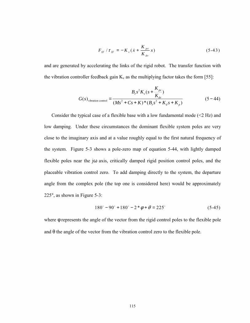
115

/ ( ) (5-43)pvIF IF v

dv

KF K x x

Kτ = − +&

and are generated by accelerating the links of the rigid robot. The transfer function with

the vibration controller feedback gain Kv as the multiplying factor takes the form [55]:

2

vibration control 2 2

( )( ) (5 44)

( )*( )

pvv

dv

d p

KB s K s

KG sMs Cs K B s K s K

τ

τ

+= −

+ + + +

Consider the typical case of a flexible base with a low fundamental mode (<2 Hz) and

low damping. Under these circumstances the dominant flexible system poles are very

close to the imaginary axis and at a value roughly equal to the first natural frequency of

the system. Figure 5-3 shows a pole-zero map of equation 5-44, with lightly damped

flexible poles near the jω axis, critically damped rigid position control poles, and the

placeable vibration control zero. To add damping directly to the system, the departure

angle from the complex pole (the top one is considered here) would be approximately

225°, as shown in Figure 5-3:

180 90 180 2 * 225 (5-45)φ θ− + − + =o o o o

where φ represents the angle of the vector from the rigid control poles to the flexible pole

and θ the angle of the vector from the vibration control zero to the flexible pole.

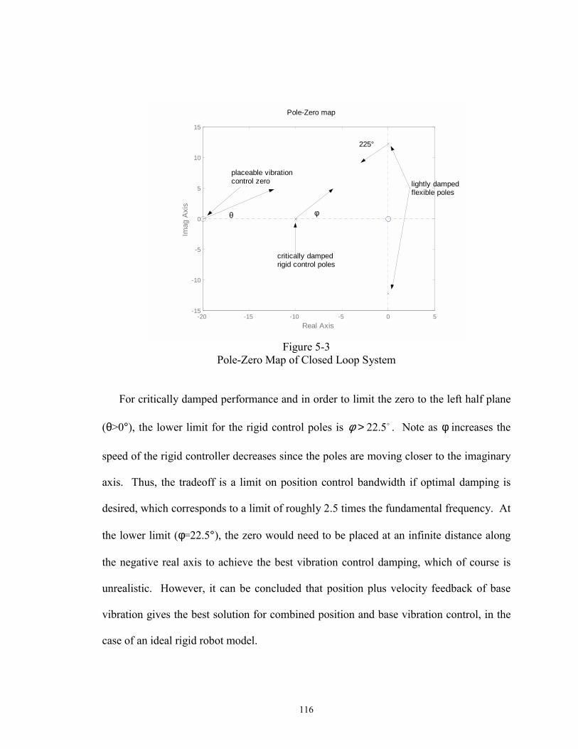
116

Pole-Zero map

-20 -15 -10 -5 0 5-15

-10

-5

0

5

10

15

Real Axis

Imag

Axi

s

225°

critically damped rigid control poles

placeable vibrationcontrol zero lightly damped

flexible poles

θ φ

Figure 5-3

Pole-Zero Map of Closed Loop System

For critically damped performance and in order to limit the zero to the left half plane

(θ>0°), the lower limit for the rigid control poles is o5.22>φ . Note as φ increases the

speed of the rigid controller decreases since the poles are moving closer to the imaginary

axis. Thus, the tradeoff is a limit on position control bandwidth if optimal damping is

desired, which corresponds to a limit of roughly 2.5 times the fundamental frequency. At

the lower limit (φ=22.5°), the zero would need to be placed at an infinite distance along

the negative real axis to achieve the best vibration control damping, which of course is

unrealistic. However, it can be concluded that position plus velocity feedback of base

vibration gives the best solution for combined position and base vibration control, in the

case of an ideal rigid robot model.

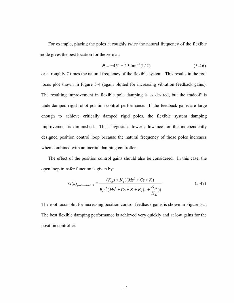
117

For example, placing the poles at roughly twice the natural frequency of the flexible

mode gives the best location for the zero at:

145 2 * tan (1/ 2) (5-46)θ −= − +o

or at roughly 7 times the natural frequency of the flexible system. This results in the root

locus plot shown in Figure 5-4 (again plotted for increasing vibration feedback gains).

The resulting improvement in flexible pole damping is as desired, but the tradeoff is

underdamped rigid robot position control performance. If the feedback gains are large

enough to achieve critically damped rigid poles, the flexible system damping

improvement is diminished. This suggests a lower allowance for the independently

designed position control loop because the natural frequency of those poles increases

when combined with an inertial damping controller.

The effect of the position control gains should also be considered. In this case, the

open loop transfer function is given by:

2

2 2

( )( )( ) (5-47)

( ( ))

d pposition control

pvv

dv

K s K Ms Cs KG s K

B s Ms Cs K K sKτ

+ + +=

+ + + +

The root locus plot for increasing position control feedback gains is shown in Figure 5-5.

The best flexible damping performance is achieved very quickly and at low gains for the

position controller.

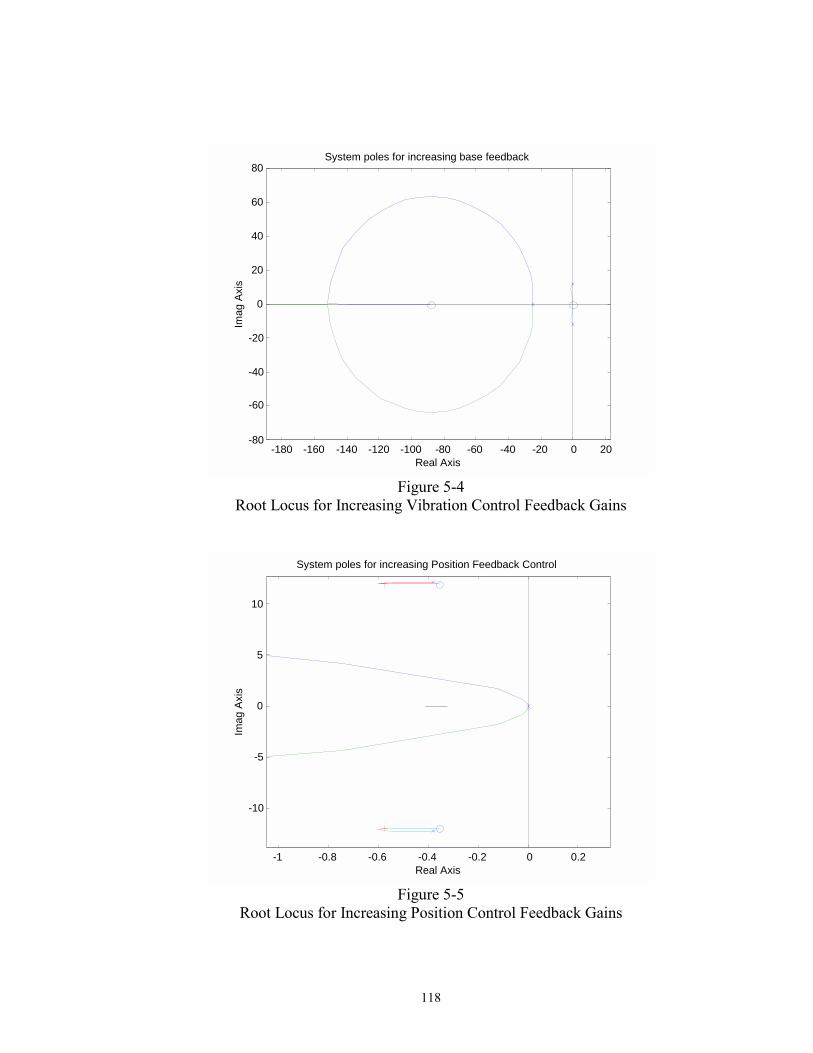
118

-180 -160 -140 -120 -100 -80 -60 -40 -20 0 20 -80

-60

-40

-20

0

20

40

60

80

Real Axis

Imag

Axi

s

System poles for increasing base feedback

Figure 5-4

Root Locus for Increasing Vibration Control Feedback Gains

-1 -0.8 -0.6 -0.4 -0.2 0 0.2

-10

-5

0

5

10

Real Axis

Imag

Axi

s

System poles for increasing Position Feedback Control

Figure 5-5

Root Locus for Increasing Position Control Feedback Gains

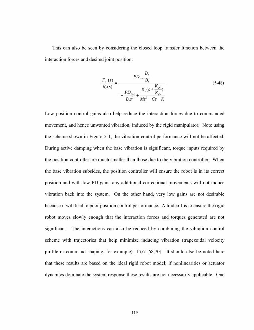
119

This can also be seen by considering the closed loop transfer function between the

interaction forces and desired joint position:

2 2

( ) (5-48)( ) ( )

1

fpos

IF

pvdv

pos dv

BPD

BF sKs K sPD K

B s Ms Cs K

τ

τ

θ=

++ +

+ +

Low position control gains also help reduce the interaction forces due to commanded

movement, and hence unwanted vibration, induced by the rigid manipulator. Note using

the scheme shown in Figure 5-1, the vibration control performance will not be affected.

During active damping when the base vibration is significant, torque inputs required by

the position controller are much smaller than those due to the vibration controller. When

the base vibration subsides, the position controller will ensure the robot is in its correct

position and with low PD gains any additional correctional movements will not induce

vibration back into the system. On the other hand, very low gains are not desirable

because it will lead to poor position control performance. A tradeoff is to ensure the rigid

robot moves slowly enough that the interaction forces and torques generated are not

significant. The interactions can also be reduced by combining the vibration control

scheme with trajectories that help minimize inducing vibration (trapezoidal velocity

profile or command shaping, for example) [15,61,68,70]. It should also be noted here

that these results are based on the ideal rigid robot model; if nonlinearities or actuator

dynamics dominate the system response these results are not necessarily applicable. One

120

representative case is discussed in Section 5.4.5 with a rigid robot dominated by

hydraulic actuators.

This indicates it is important to maintain separation of the performance of the two

control loops. The work shown here is a quick overview of the controller under typical

operating conditions. However, the position controller can interfere with the vibration

controller, as shown in Figure 5-6. In this case, the flexible system poles are drawn

towards the real axis, as desired. However, the position control poles are drawn towards

zero, which results in poor rigid robot control performance with increasing vibration

control feedback gains.

When the critically damped rigid position control poles are chosen at the natural

frequency of the flexible system and the zero chosen to cancel it, good performance

results for both position and vibration control, as can be seen in Figure 5-7. With a given

set of PD position control gains, the vibration control feedback gains can be selected to

achieve the desired effect of increased damping of the lightly damped flexible poles

while minimizing impact on the position control poles. In reality, perfect cancellation

would not occur, but the impact is minimal and in the form of slightly reduced damping

improvement or slight underdamped position control performance, as shown in Figures 5-

8 and 5-9.

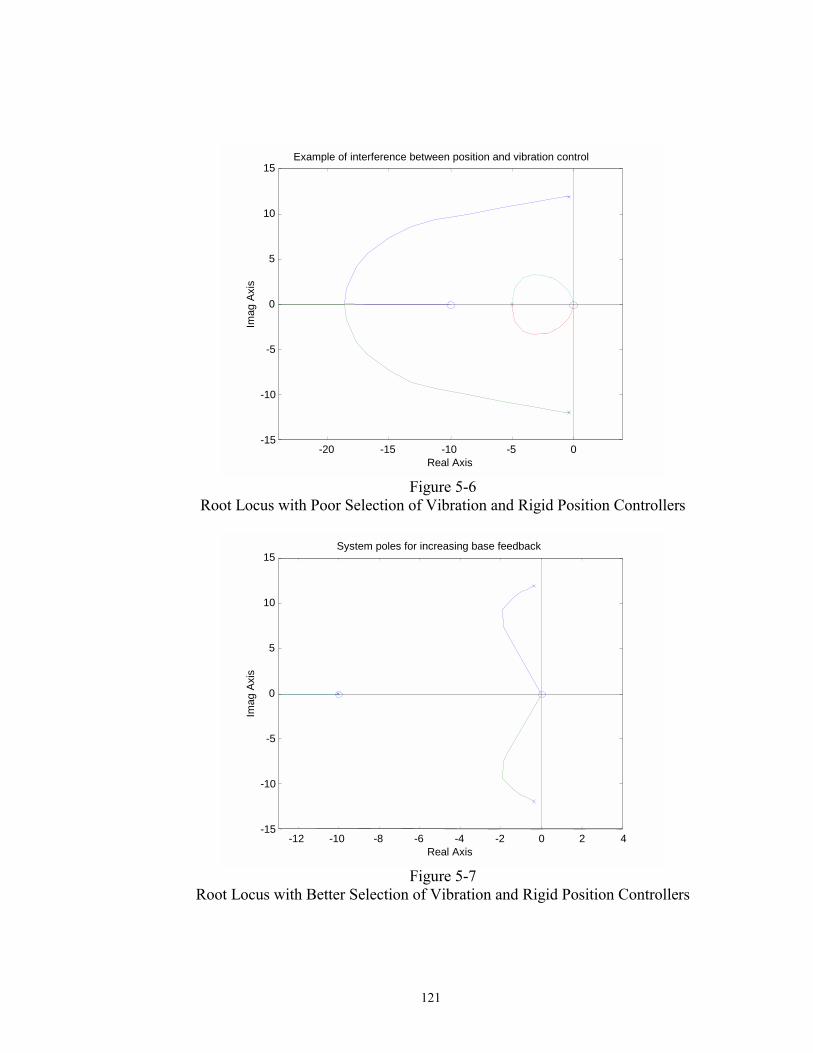
121

-20 -15 -10 -5 0 -15

-10

-5

0

5

10

15

Real Axis

Imag

Axi

s

Example of interference between position and vibration control

Figure 5-6

Root Locus with Poor Selection of Vibration and Rigid Position Controllers

-12 -10 -8 -6 -4 -2 0 2 4 -15

-10

-5

0

5

10

15

Real Axis

Imag

Axi

s

System poles for increasing base feedback

Figure 5-7

Root Locus with Better Selection of Vibration and Rigid Position Controllers

122

-25 -20 -15 -10 -5 0 5-15

-10

-5

0

5

10

15

Real Axis

Imag

Axi

s

Systen poles for increasing base feedback gains

Figure 5-8

Effect of Choosing Vibration Control Zero too Large

-12 -10 -8 -6 -4 -2 0 2 4-15

-10

-5

0

5

10

15

Real Axis

Imag

Axi

s

System poles for increasing base feedback gains

Figure 5-9

Effects of Choosing Vibration Control Zero too Small

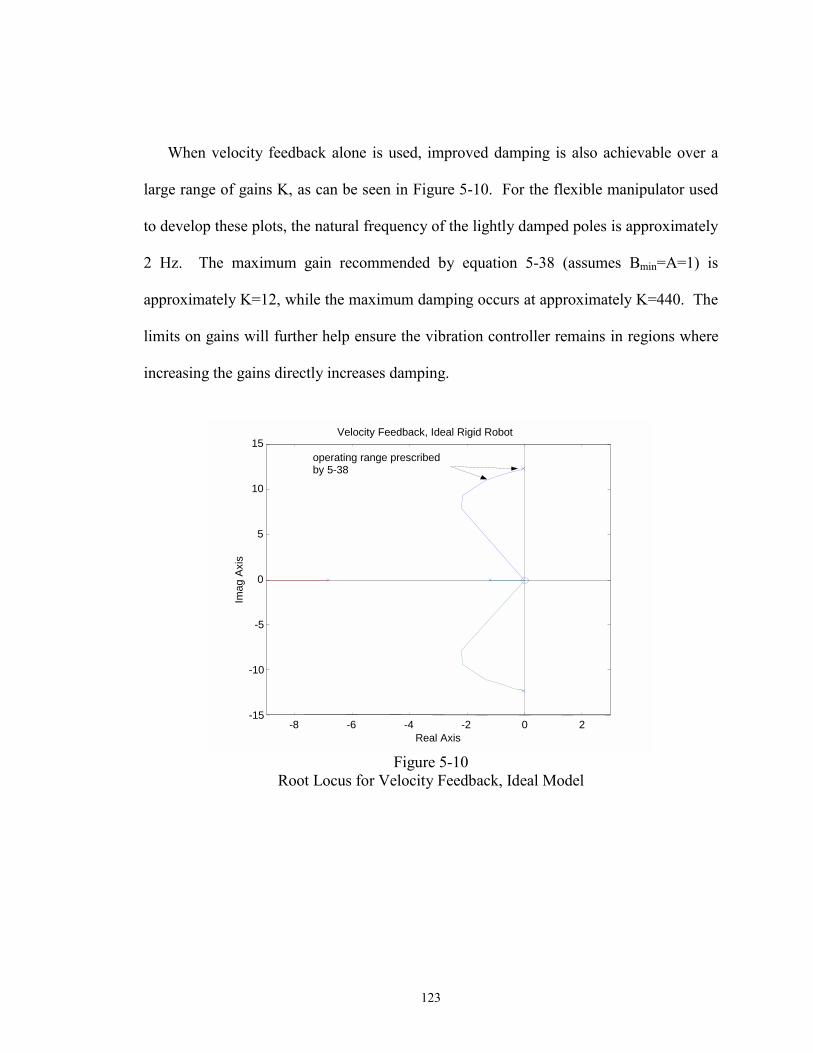
123

When velocity feedback alone is used, improved damping is also achievable over a

large range of gains K, as can be seen in Figure 5-10. For the flexible manipulator used

to develop these plots, the natural frequency of the lightly damped poles is approximately

2 Hz. The maximum gain recommended by equation 5-38 (assumes Bmin=A=1) is

approximately K=12, while the maximum damping occurs at approximately K=440. The

limits on gains will further help ensure the vibration controller remains in regions where

increasing the gains directly increases damping.

-8 -6 -4 -2 0 2 -15

-10

-5

0

5

10

15

Real Axis

Imag

Axi

s

Velocity Feedback, Ideal Rigid Robot

operating range prescribedby 5-38

Figure 5-10

Root Locus for Velocity Feedback, Ideal Model

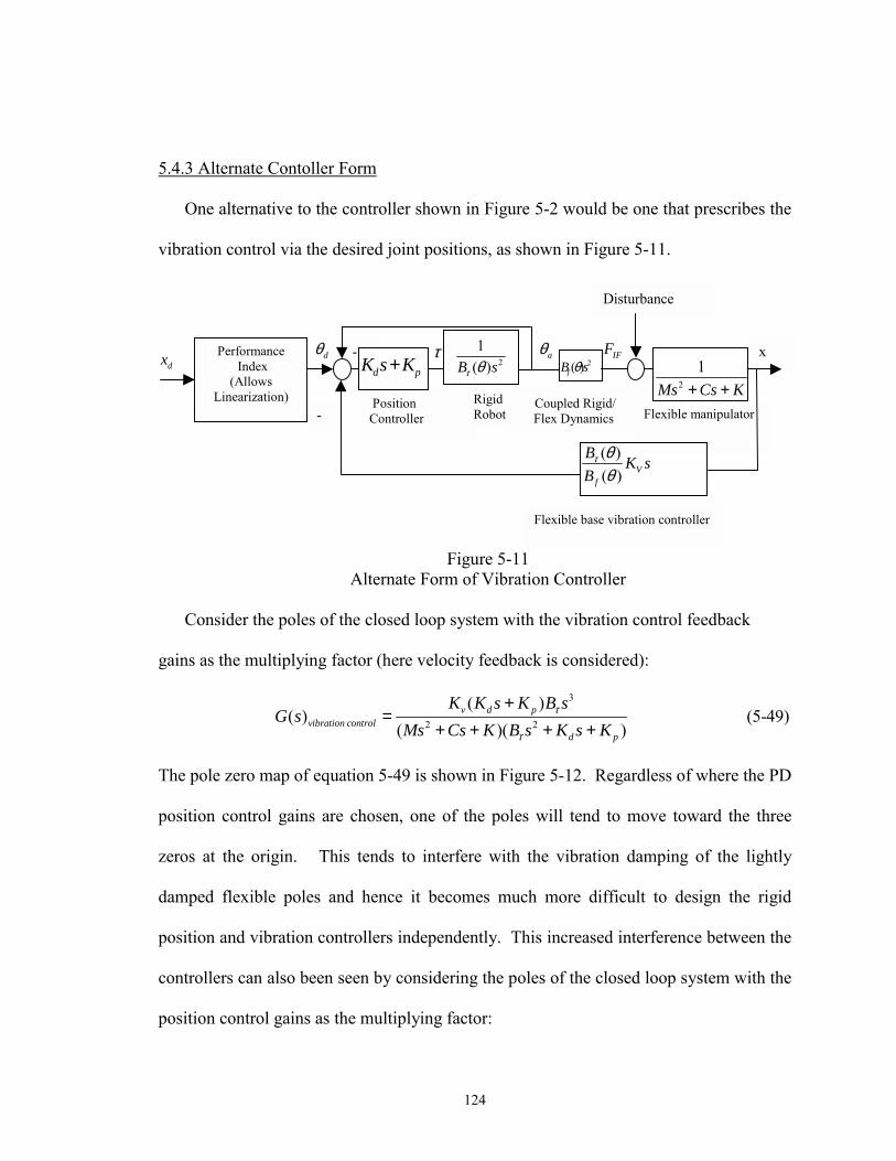
124

5.4.3 Alternate Contoller Form

One alternative to the controller shown in Figure 5-2 would be one that prescribes the

vibration control via the desired joint positions, as shown in Figure 5-11.

Figure 5-11 Alternate Form of Vibration Controller

Consider the poles of the closed loop system with the vibration control feedback

gains as the multiplying factor (here velocity feedback is considered):

3

2 2

( )( ) (5-49)

( )( )v d p

vibration controld p

K K s K B sG s

Ms Cs K B s K s Kτ

τ

+=

+ + + +

The pole zero map of equation 5-49 is shown in Figure 5-12. Regardless of where the PD

position control gains are chosen, one of the poles will tend to move toward the three

zeros at the origin. This tends to interfere with the vibration damping of the lightly

damped flexible poles and hence it becomes much more difficult to design the rigid

position and vibration controllers independently. This increased interference between the

controllers can also been seen by considering the poles of the closed loop system with the

position control gains as the multiplying factor:

Flexible base vibration controller

-

Disturbance

Coupled Rigid/ Flex Dynamics Flexible manipulator

x -

- Position Controller

Performance

Index (Allows

Linearization)

Rigid Robot

2

1( )B sτ θdx dθ

d pK s K+τ aθ

2( )fB sθIFF

2

1Ms Cs K+ +

( )( ) V

f

B K sBτ θθ

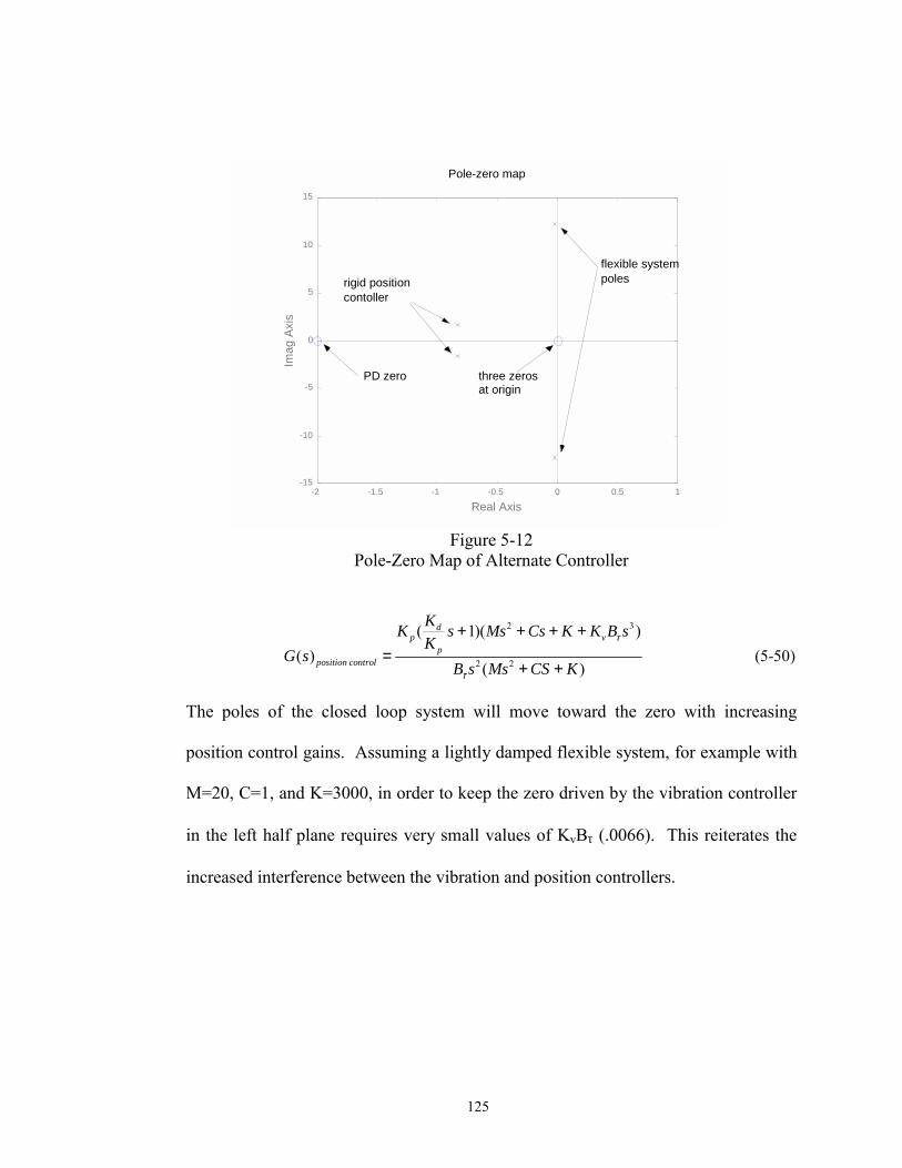
125

Pole-zero map

-2 -1.5 -1 -0.5 0 0.5 1 -15

-10

-5

0

5

10

15

Real Axis

Imag

Axi

s flexible system poles rigid position

contoller

PD zero three zerosat origin

Figure 5-12

Pole-Zero Map of Alternate Controller

2 3

2 2

( 1)( )( ) (5-50)

( )

dp v

pposition control

KK s Ms Cs K K B sK

G sB s Ms CS K

τ

τ

+ + + +=

+ +

The poles of the closed loop system will move toward the zero with increasing

position control gains. Assuming a lightly damped flexible system, for example with

M=20, C=1, and K=3000, in order to keep the zero driven by the vibration controller

in the left half plane requires very small values of KvBτ (.0066). This reiterates the

increased interference between the vibration and position controllers.

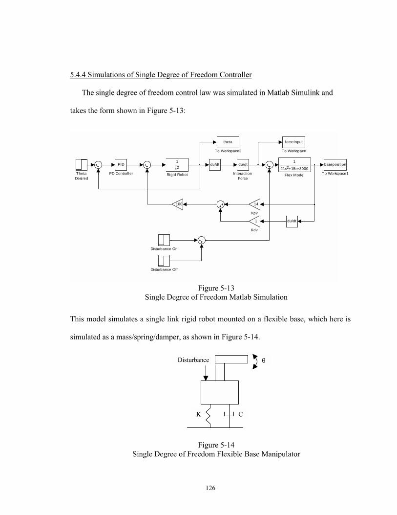
126

5.4.4 Simulations of Single Degree of Freedom Controller

The single degree of freedom control law was simulated in Matlab Simulink and

takes the form shown in Figure 5-13:

Figure 5-13 Single Degree of Freedom Matlab Simulation

This model simulates a single link rigid robot mounted on a flexible base, which here is

simulated as a mass/spring/damper, as shown in Figure 5-14.

Figure 5-14

Single Degree of Freedom Flexible Base Manipulator

θ

C

Disturbance

K

theta

To Workspace2

baseposition

To Workspace1

forceinput

To Workspace

ThetaDesired

1

s 2

Rigid Robot

PID

PD Controller

14

Kpv

1

Kdv

100

du/dt

Interaction Force

1

21s +15s+30002

Flex Model

du/dt

Disturbance On

Disturbance Off

du/dt

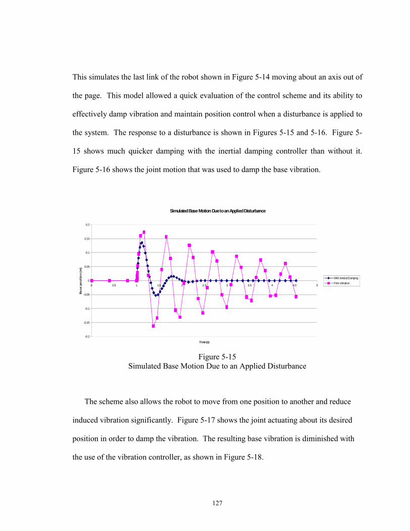
127

This simulates the last link of the robot shown in Figure 5-14 moving about an axis out of

the page. This model allowed a quick evaluation of the control scheme and its ability to

effectively damp vibration and maintain position control when a disturbance is applied to

the system. The response to a disturbance is shown in Figures 5-15 and 5-16. Figure 5-

15 shows much quicker damping with the inertial damping controller than without it.

Figure 5-16 shows the joint motion that was used to damp the base vibration.

Simulated Base Motion Due to an Applied Disturbance

-0.2

-0.15

-0.1

-0.05

0

0.05

0.1

0.15

0.2

0 0.5 1 1.5 2 2.5 3 3.5 4 4.5 5

Time (s)

Base

pos

itio

n (m

)

With Inertial Damping

Free vibration

Figure 5-15

Simulated Base Motion Due to an Applied Disturbance

The scheme also allows the robot to move from one position to another and reduce

induced vibration significantly. Figure 5-17 shows the joint actuating about its desired

position in order to damp the vibration. The resulting base vibration is diminished with

the use of the vibration controller, as shown in Figure 5-18.

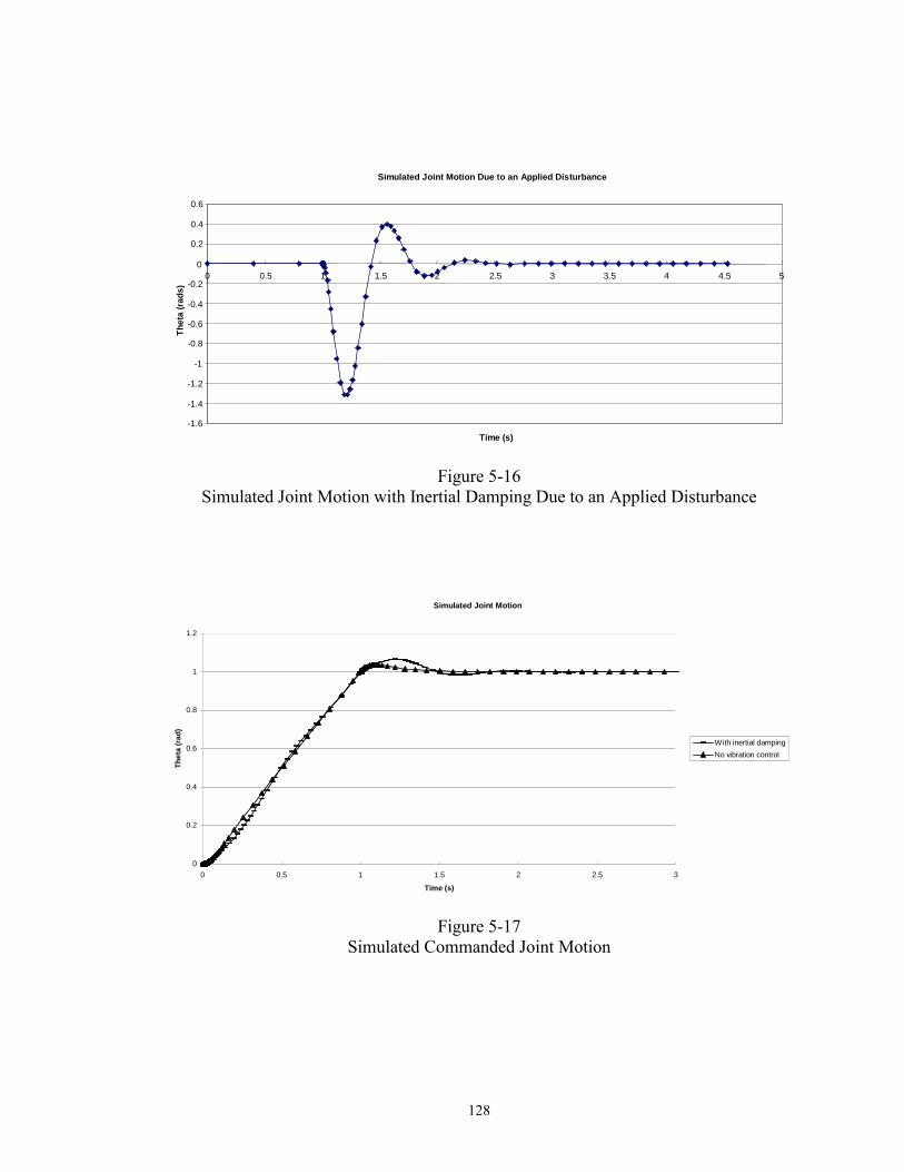
128

Simulated Joint Motion Due to an Applied Disturbance

-1.6

-1.4

-1.2

-1

-0.8

-0.6

-0.4

-0.2

0

0.2

0.4

0.6

0 0.5 1 1.5 2 2.5 3 3.5 4 4.5 5

Time (s)

Thet

a (r

ads)

Figure 5-16

Simulated Joint Motion with Inertial Damping Due to an Applied Disturbance

Simulated Joint Motion

0

0.2

0.4

0.6

0.8

1

1.2

0 0.5 1 1.5 2 2.5 3

Time (s)

Thet

a (r

ad)

With inertial dampingNo vibration control

Figure 5-17

Simulated Commanded Joint Motion

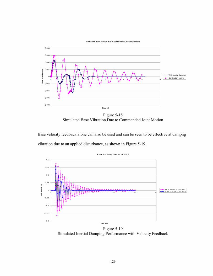
129

Simulated Base motion due to commanded joint movement

-0.008

-0.006

-0.004

-0.002

0

0.002

0.004

0.006

0.008

0 1 2 3 4 5 6

Time (s)

Bas

e po

sitio

n (m

)

With inertial dampingNo vibration control

Figure 5-18

Simulated Base Vibration Due to Commanded Joint Motion

Base velocity feedback alone can also be used and can be seen to be effective at dampng

vibration due to an applied disturbance, as shown in Figure 5-19.

B a s e v e l o c i t y f e e d b a c k o n l y

- 0 . 2

- 0 . 1 5

- 0 . 1

- 0 . 0 5

0

0 . 0 5

0 . 1

0 . 1 5

0 . 2

0 5 1 0 1 5 2 0 2 5

T im e ( s )

Bas

e po

sitio

n (m

)

N o V ib r a t io n C o n t r o lW i t h In e r t ia l D a m p in g

Figure 5-19 Simulated Inertial Damping Performance with Velocity Feedback

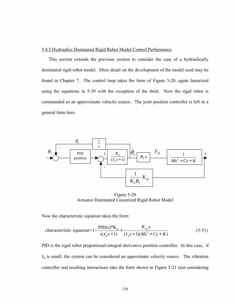
130

5.4.5 Hydraulics Dominated Rigid Robot Model Control Performance

This section extends the previous section to consider the case of a hydraulically

dominated rigid robot model. More detail on the development of the model used may be

found in Chapter 7. The control loop takes the form of Figure 5-20, again linearized

using the equations in 5-39 with the exception of the third. Now the rigid robot is

commanded as an approximate velocity source. The joint position controller is left in a

general form here.

Figure 5-20

Actuator Dominated Linearized Rigid Robot Model

Now the characteristic equation takes the form:

h2

PID(s)*K =1+ (5-51)( 1) ( 1)( )

pv

d d

K scharacteristic equation

s s s Ms Cs Kτ τ+

+ + + +

PID is the rigid robot proportional-integral-derivative position controller. In this case, if

τd is small, the system can be considered an appoximate velocity source. The vibration

controller and resulting interactions take the form shown in Figure 5-21 (not considering

x

-

-

aθ&PID position

dθ τ( 1)

h

d

Ksτ +

IFFfB s

KCsMs ++2

1

1pv

h f

KK B

1s

aθ

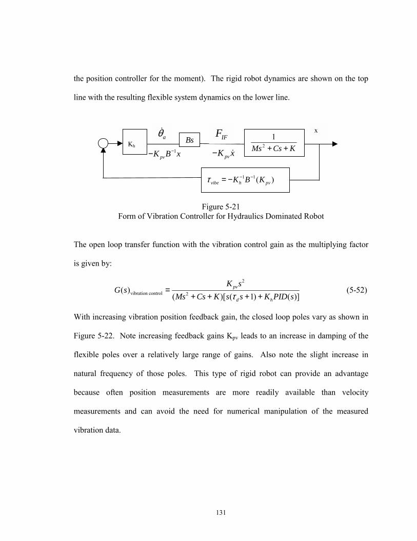
131

the position controller for the moment). The rigid robot dynamics are shown on the top

line with the resulting flexible system dynamics on the lower line.

Figure 5-21

Form of Vibration Controller for Hydraulics Dominated Robot

The open loop transfer function with the vibration control gain as the multiplying factor

is given by:

2

vibration control 2( ) (5-52)( )[ ( 1) ( )]

pv

d h

K sG s

Ms Cs K s s K PID sτ=

+ + + +

With increasing vibration position feedback gain, the closed loop poles vary as shown in

Figure 5-22. Note increasing feedback gains Kpv leads to an increase in damping of the

flexible poles over a relatively large range of gains. Also note the slight increase in

natural frequency of those poles. This type of rigid robot can provide an advantage

because often position measurements are more readily available than velocity

measurements and can avoid the need for numerical manipulation of the measured

vibration data.

x aθ&

Kh

IFFBs

KCsMs ++2

1

1 1( )vibe h pvK B Kτ − −= −

pvK x− &1pvK B x−−

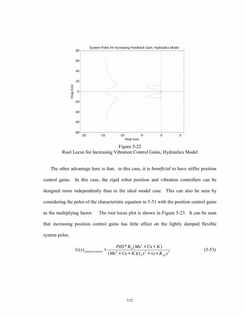
132

-20 -15 -10 -5 0 5 -80

-60

-40

-20

0

20

40

60

80

Real Axis

Imag

Axi

s

System Poles for Increasing Feedback Gain, Hydraulics Model M d l

Figure 5-22

Root Locus for Increasing Vibration Control Gains, Hydraulics Model

The other advantage here is that, in this case, it is beneficial to have stiffer position

control gains. In this case, the rigid robot position and vibration controllers can be

designed more independently than in the ideal model case. This can also be seen by

considering the poles of the characteristic equation in 5-51 with the position control gains

as the multiplying factor. The root locus plot is shown in Figure 5-23. It can be seen

that increasing position control gains has little effect on the lightly damped flexible

system poles.

2

2 2 2

* ( )( ) (5-53)( )( )

hposition control

d pv

PID K Ms Cs KG sMs Cs K s s K sτ

+ +=+ + + +

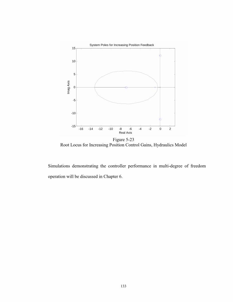
133

-16 -14 -12 -10 -8 -6 -4 -2 0 2 -15

-10

-5

0

5

10

15

Real Axis

Imag

Axi

s

System Poles for Increasing Position Feedback

Figure 5-23

Root Locus for Increasing Position Control Gains, Hydraulics Model

Simulations demonstrating the controller performance in multi-degree of freedom

operation will be discussed in Chapter 6.

134

CHAPTER VI

SIMULATIONS

6.1 Introduction

Simulations were built in Matlab to test the ability of the control scheme to damp

vibration in multi-degrees of freedom. A macromanipulator was modeled assuming three

degrees of freedom of vibration and using a recursive Lagrangian technique as described

in Section 3.2. Two modes of transverse vibration were assumed in each planar

direction. In order to add a sense of realism to the simulation, the third mode in the z

direction was chosen based on assumed modes for torsional vibration. This was chosen

since torsional vibration is common for flexible links and, although it is not a concern for

single link macromanipulators, it will be a concern for multi-link manipulators. In

addition, since torsional vibration is at a higher frequency than transverse vibration, it

allowed an early assessment of the ability of the scheme to operate over a wide range of

frequencies. The resulting equations of motion for the flexible base take the form of

equation 3-19 with constant matrices. A three degree of freedom rigid robot was used for

damping and takes the form of the last equation in 3-27, while the interactions are given

by equation 4-1. The purpose of these simulations was to test the controller and gain

limits discussed in Chapter 5. In addition, the usefulness of the performance index

135

described in Section 5.2 was tested to determine joint configurations better suited for

inertial damping.

The simulations were extended to the case of a two link flexible manipulator with a

six degree of freedom anthropomorphic/wrist micromanipulator. The flexible base

parameters were designed to give base motion similar to the two link experimental

testbed, discussed in Chapter 7. The modes modeled in the first link were four transverse

modes and one torsional mode, and one transverse mode was modeled in the second link.

The complexity of this model made the simulation time extremely long. It was decided

the three degree of freedom simulation with additional higher frequency modes added

would suffice to study multi-degree of freedom vibration damping and sufficiently

represented the testbed. Thus, the baseline simulations used primarily in this study had

three degrees of freedom of base vibration and used a three degree of freedom rigid robot

to provide the vibration damping.

Finally, an alternate configuration of a rigid robot with performance dominated by

hydraulic actuators was studied. As discussed in Chapter 5, with a small change to the

control scheme the controller performance is nearly identical to that of the ideal rigid

robot performance. However, the effect of variation in actuator performance can add

much more uncertainty to the system than the equivalent seen with the ideally modeled

robot with nonlinearities. In particular, the effect of increasing the servovalve time

constant and higher order dynamics were investigated in simulation, primarily prompted

by issues that manifested during laboratory testing.

136

6.2 Single Flexible Link Macromanipulator with Anthropomorphic Rigid Robot

The overall schematic of the three degree of freedom simulation is shown in Figure 6-

1. Starting at the left of the model, trajectory inputs in the form of desired joint

trajectories are the inputs to the rigid robot. The trajectory inputs were either constant

joint positions, used to test the response of the vibration controller to a disturbance input,

or point-to-point trajectories. In order to test the use of the performance index in

predicting inertial damping performance, point-to-point trajectories were generated from

desired starting and end points. For each end point in the workspace, there are multiple

joint space configurations that can be used to reach it (provided the robot is not operating

at a kinematic singularity, which is assumed for this work). In each case, one of the joint

configurations gives predicted better inertial damping performance than the other ones.

Thus, two tracks were compared in these simulations; one is the track given by the

beginning and end points in the better joint space configurations, and the other is the

alternate joint space configuration track.

The rigid robot model was written in the form of an s-function [21], which gives more

flexibility in developing the system model and allows modeling nonlinearities. The

inputs to the rigid robot are the controller torques, which consist of the PID position

control torques plus the additional contribution due to the vibration controller. The total

input to each joint is given by:

( ) ( ) (6-1)d a aPID ID Kτ = − −θ θ θ x&

where PID is an independent proportional-integral-derivative controller (or some

variation such as PI or PD), ID is the inverse dynamics function defined in Equation 5-8,

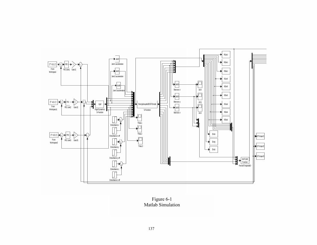
137

Figure 6-1 Matlab Simulation

accz

accy

accx

IDTorqueJ3

Disty

Distz

Distx

th3acc

th2acc

th1acc

th3vel

th2vel

th1vel

th3out

IDTorqueJ2

IDTorqueJ1

th2out

th1out

Theta 3

Theta 2

Theta 1

flexrigidcoupled3DOF2mode

S-Function

rigid

Rigid DynamicsS-Function

PID

PID Joint3

PID

PID Joint2

PID

PID Joint1

du/dt

Joint 3 acceleration

du/dt

Joint 2 acceleration

du/dt

Joint 1 acceleration

1

GainJ3

1

GainJ2

1

GainJ1

[T' U(3,:)']

FromWorkspace2

[T' U(2,:)']

FromWorkspace1

[T' U(1,:)']

FromWorkspace

MATLABFunction

Forces/Torques&ID

Disturbance z off

Disturbance z

Disturbance y off

Disturbance y

Disturbance x off

Disturbance x

em

mem

mdu/dt

Base acc z

du/dt

Base acc y

du/dt

Base acc x

138

and K is the vibration control feedback gains. For these simulations, a reduced inverse

dynamics function consisting of only the interaction force effects was used, or

1( ) ( ) ( ) (6-2)fID B Bτ−=θ θ θ

The output of the rigid dynamics s-function are the states of the rigid robot, which are the

joint positions and velocities. The joint positions are fed back to the PID controller. The

joint velocities are differentiated to yield the joint accelerations and used to calculate the

interaction forces and torques, given by equation 4-1.

The flexible base is also modeled using equation 3-19 as an s-function, with inputs

the interactions due to the rigid robot. There is also an option to apply a disturbance

directly to the flexible base. Since the states of the flexible base are the generalized

coordinates, the disturbances applied in each direction are applied to all of the states

governing the motion in that direction. For example, an applied disturbance in the x

direction is applied to all of the generalized coordinates that affect the motion in that

direction. The states are the generalized coordinates and their rates, while the outputs are

the overall base motion in the x, y and z directions and their derivatives. The applied

distubances and interaction forces and torques are also output and recorded. All of the

states and variables are sent to the workspace where they can be stored and analyzed

later.

The mass, damping, and stiffness properties of the macromanipulator were

determined as described in section 3.2 and are given by the 5x5 matrices M, C, and K

from equation 3-19. The fully coupled system mass matrix representing the inertia

properties of the coupled system is given by:

139

1 (6-3)T f fM M A B B Aτ τ−= + +

where the coupling matrices are given by the appropriate equations in Appendix A. In

order to form these equations in the typical state space form, the state matrix is defined

as:

1 1

(6-4)T TM C M KA

I Z

− − − −=

where I is the 5x5 identity matrix and Z is a 5x5 matrix of zeros. The system states are

given by:

[ ]1 2 1 2 1 1 2 1 2 1 (6-5)Tp p q q s p p q q s=x & & & & &

where p1 and p2 are generalized coordinates representing two transverse modes in the x

direction, q1 and q2 represent two transverse modes in the y direction, and s1 represents a

torsional mode of vibration.

The input to the system is defined as:

1 1

(6-6)

T TM MInput

CZ

− − +=

F D

where CZ is a column of five zeros. D are disturbances that can be directly applied to the

system generalized coordinates and F is the 5x1 set of interaction forces and torques. For

most of the baseline simulations, only the interaction forces were calculated, but for some

simulations both interaction forces and torques were included as discussed in Section

6.3.2. In the general case, F is given by:

iIFi

z=L

+ ( ) (6-7)zIFiF φ τ∂=∂

F

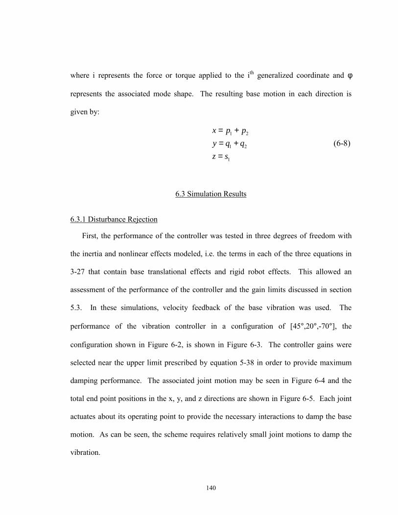
140

where i represents the force or torque applied to the ith generalized coordinate and φ

represents the associated mode shape. The resulting base motion in each direction is

given by:

1 2

1 2

1

(6-8)x p py q qz s

= += +=

6.3 Simulation Results 6.3.1 Disturbance Rejection

First, the performance of the controller was tested in three degrees of freedom with

the inertia and nonlinear effects modeled, i.e. the terms in each of the three equations in

3-27 that contain base translational effects and rigid robot effects. This allowed an

assessment of the performance of the controller and the gain limits discussed in section

5.3. In these simulations, velocity feedback of the base vibration was used. The

performance of the vibration controller in a configuration of [45°,20°,-70°], the

configuration shown in Figure 6-2, is shown in Figure 6-3. The controller gains were

selected near the upper limit prescribed by equation 5-38 in order to provide maximum

damping performance. The associated joint motion may be seen in Figure 6-4 and the

total end point positions in the x, y, and z directions are shown in Figure 6-5. Each joint

actuates about its operating point to provide the necessary interactions to damp the base

motion. As can be seen, the scheme requires relatively small joint motions to damp the

vibration.

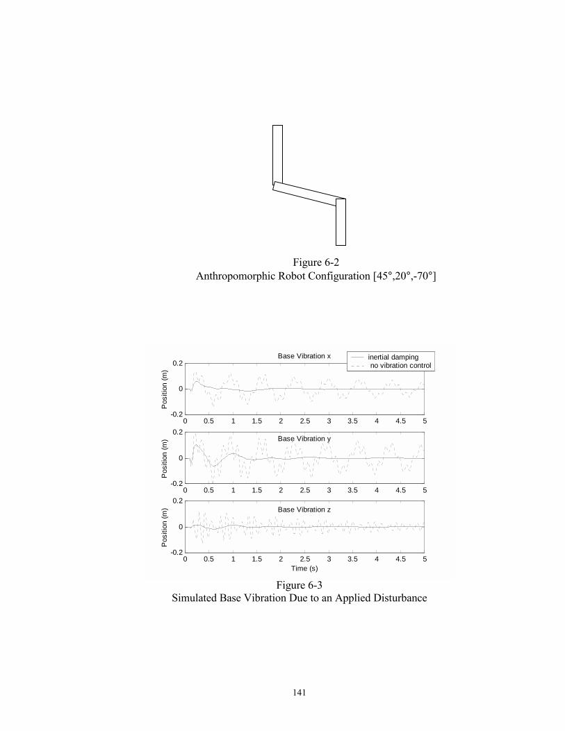
141

Figure 6-2

Anthropomorphic Robot Configuration [45°,20°,-70°]

0 0.5 1 1.5 2 2.5 3 3.5 4 4.5 5-0.2

0

0.2Base Vibration x

Pos

ition

(m)

0 0.5 1 1.5 2 2.5 3 3.5 4 4.5 5-0.2

0

0.2

Pos

ition

(m) Base Vibration y

inertial damping no vibration control

0 0.5 1 1.5 2 2.5 3 3.5 4 4.5 5-0.2

0

0.2Base Vibration z

Time (s)

Pos

ition

(m)

Figure 6-3

Simulated Base Vibration Due to an Applied Disturbance

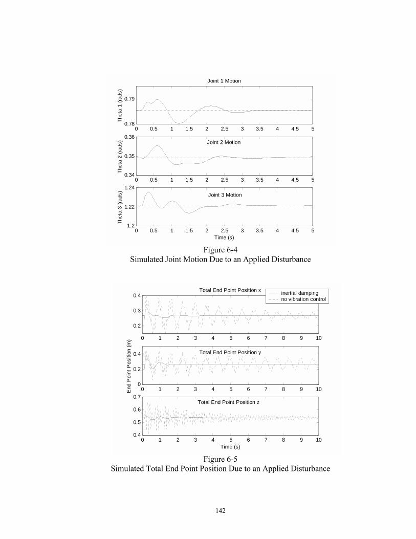
142

0 0.5 1 1.5 2 2.5 3 3.5 4 4.5 50.78

0.79

Joint 1 Motion

Thet

a 1

(rads

)

0 0.5 1 1.5 2 2.5 3 3.5 4 4.5 50.34

0.35

0.36Joint 2 Motion

Thet

a 2

(rads

)

0 0.5 1 1.5 2 2.5 3 3.5 4 4.5 51.2

1.22

1.24Joint 3 Motion

Time (s)

Thet

a 3

(rads

)

Figure 6-4

Simulated Joint Motion Due to an Applied Disturbance

0 1 2 3 4 5 6 7 8 9 10

0.2

0.3

0.4Total End Point Position x

0 1 2 3 4 5 6 7 8 9 100

0.2

0.4 Total End Point Position y

End

Poi

nt P

ositi

on (m

)

0 1 2 3 4 5 6 7 8 9 100.4

0.5

0.6

0.7Total End Point Position z

Time (s)

inertial damping no vibration control

Figure 6-5

Simulated Total End Point Position Due to an Applied Disturbance

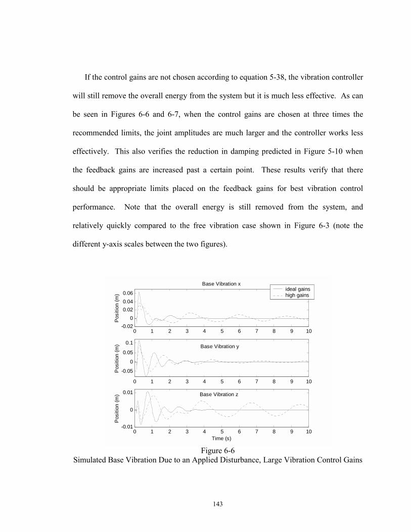
143

If the control gains are not chosen according to equation 5-38, the vibration controller

will still remove the overall energy from the system but it is much less effective. As can

be seen in Figures 6-6 and 6-7, when the control gains are chosen at three times the

recommended limits, the joint amplitudes are much larger and the controller works less

effectively. This also verifies the reduction in damping predicted in Figure 5-10 when

the feedback gains are increased past a certain point. These results verify that there

should be appropriate limits placed on the feedback gains for best vibration control

performance. Note that the overall energy is still removed from the system, and

relatively quickly compared to the free vibration case shown in Figure 6-3 (note the

different y-axis scales between the two figures).

0 1 2 3 4 5 6 7 8 9 10-0.02

00.020.040.06

Base Vibration x

Pos

ition

(m)

0 1 2 3 4 5 6 7 8 9 10

-0.05

0

0.05

0.1Base Vibration y

Pos

ition

(m)

0 1 2 3 4 5 6 7 8 9 10-0.01

0

0.01 Base Vibration z

Time (s)

Pos

ition

(m)

ideal gainshigh gains

Figure 6-6

Simulated Base Vibration Due to an Applied Disturbance, Large Vibration Control Gains

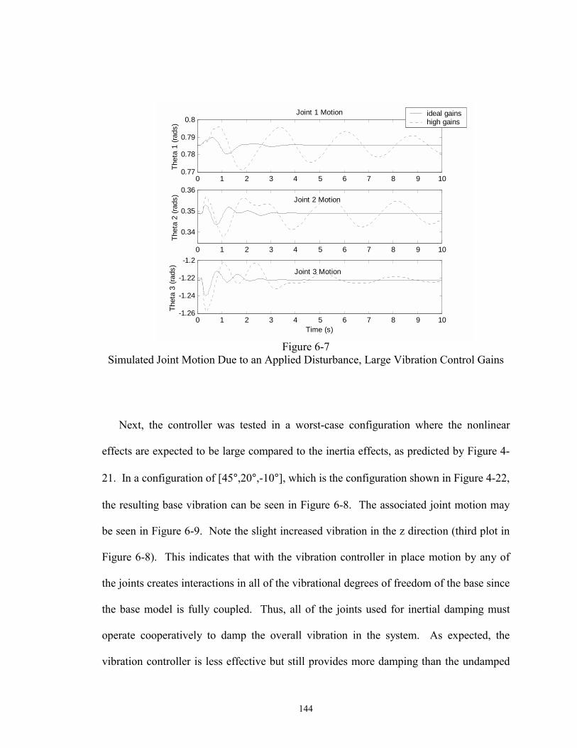
144

0 1 2 3 4 5 6 7 8 9 100.77

0.78

0.79

0.8Joint 1 Motion

Thet

a 1

(rads

)

0 1 2 3 4 5 6 7 8 9 10

0.34

0.35

0.36Joint 2 Motion

Thet

a 2

(rads

)

0 1 2 3 4 5 6 7 8 9 10-1.26

-1.24

-1.22

-1.2Joint 3 Motion

Time (s)

Thet

a 3

(rads

)

ideal gainshigh gains

Figure 6-7

Simulated Joint Motion Due to an Applied Disturbance, Large Vibration Control Gains

Next, the controller was tested in a worst-case configuration where the nonlinear

effects are expected to be large compared to the inertia effects, as predicted by Figure 4-

21. In a configuration of [45°,20°,-10°], which is the configuration shown in Figure 4-22,

the resulting base vibration can be seen in Figure 6-8. The associated joint motion may

be seen in Figure 6-9. Note the slight increased vibration in the z direction (third plot in

Figure 6-8). This indicates that with the vibration controller in place motion by any of

the joints creates interactions in all of the vibrational degrees of freedom of the base since

the base model is fully coupled. Thus, all of the joints used for inertial damping must

operate cooperatively to damp the overall vibration in the system. As expected, the

vibration controller is less effective but still provides more damping than the undamped

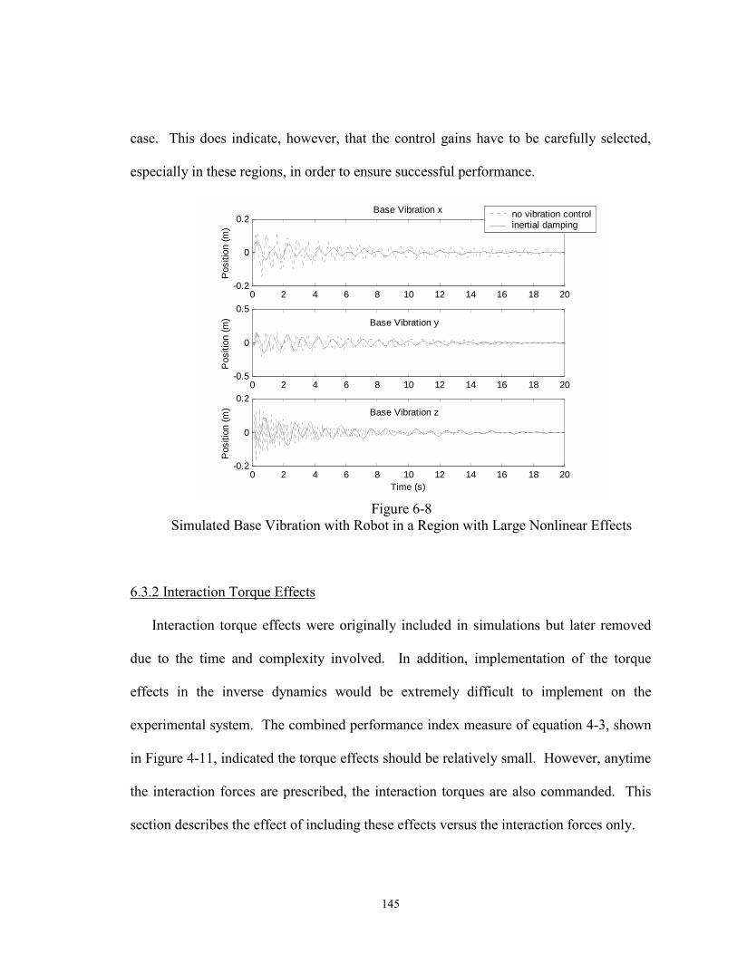
145

case. This does indicate, however, that the control gains have to be carefully selected,

especially in these regions, in order to ensure successful performance.

0 2 4 6 8 10 12 14 16 18 20-0.2

0

0.2Base Vibration x

Pos

ition

(m)

0 2 4 6 8 10 12 14 16 18 20-0.5

0

0.5Base Vibration y

Pos

ition

(m)

no vibration controlinertial damping

0 2 4 6 8 10 12 14 16 18 20-0.2

0

0.2Base Vibration z

Time (s)

Pos

ition

(m)

Figure 6-8

Simulated Base Vibration with Robot in a Region with Large Nonlinear Effects

6.3.2 Interaction Torque Effects

Interaction torque effects were originally included in simulations but later removed

due to the time and complexity involved. In addition, implementation of the torque

effects in the inverse dynamics would be extremely difficult to implement on the

experimental system. The combined performance index measure of equation 4-3, shown

in Figure 4-11, indicated the torque effects should be relatively small. However, anytime

the interaction forces are prescribed, the interaction torques are also commanded. This

section describes the effect of including these effects versus the interaction forces only.

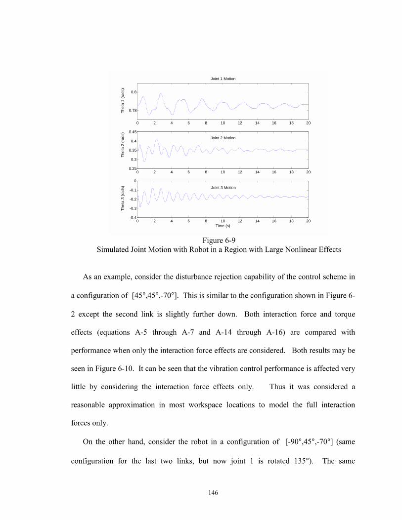
146

0 2 4 6 8 10 12 14 16 18 20 0.78

0.8

Joint 1 Motion

Thet

a 1

(rads

)

0 2 4 6 8 10 12 14 16 18 20 0.25 0.3

0.35 0.4

0.45 Joint 2 Motion

Thet

a 2

(rads

)

0 2 4 6 8 10 12 14 16 18 20 -0.4 -0.3 -0.2 -0.1

0 Joint 3 Motion

Time (s)

Thet

a 3

(rads

)

Figure 6-9

Simulated Joint Motion with Robot in a Region with Large Nonlinear Effects

As an example, consider the disturbance rejection capability of the control scheme in

a configuration of [45°,45°,-70°]. This is similar to the configuration shown in Figure 6-

2 except the second link is slightly further down. Both interaction force and torque

effects (equations A-5 through A-7 and A-14 through A-16) are compared with

performance when only the interaction force effects are considered. Both results may be

seen in Figure 6-10. It can be seen that the vibration control performance is affected very

little by considering the interaction force effects only. Thus it was considered a

reasonable approximation in most workspace locations to model the full interaction

forces only.

On the other hand, consider the robot in a configuration of [-90°,45°,-70°] (same

configuration for the last two links, but now joint 1 is rotated 135°). The same

147

comparison is made and shown in Figure 6-11. The vibration controller still removes

energy from the system in both cases, but the performance with and without the

interaction torques is very different. An area of future research is recommended to

investigate in more detail the interaction torques and determine appropriate

simplifications to enable modeling them in a reasonable manner for simulation and

experimental implementation. One possible reason for this change in performance is

discussed in Section 7.5.3.

0 1 2 3 4 5 6 7 8 9 10-0.1

0

0.1Vibration x

Pos

ition

(m)

0 1 2 3 4 5 6 7 8 9 10-0.2

0

0.2Vibration y

Pos

ition

(m)

0 1 2 3 4 5 6 7 8 9 10-0.01

0

0.01

0.02Vibration z

Time (s)

Pos

ition

(m)

Forces Forces and Torques

Figure 6-10

Simulated Base Vibration with Interaction Forces and Torques Modeled, Configuration [45°,45°,-70°]

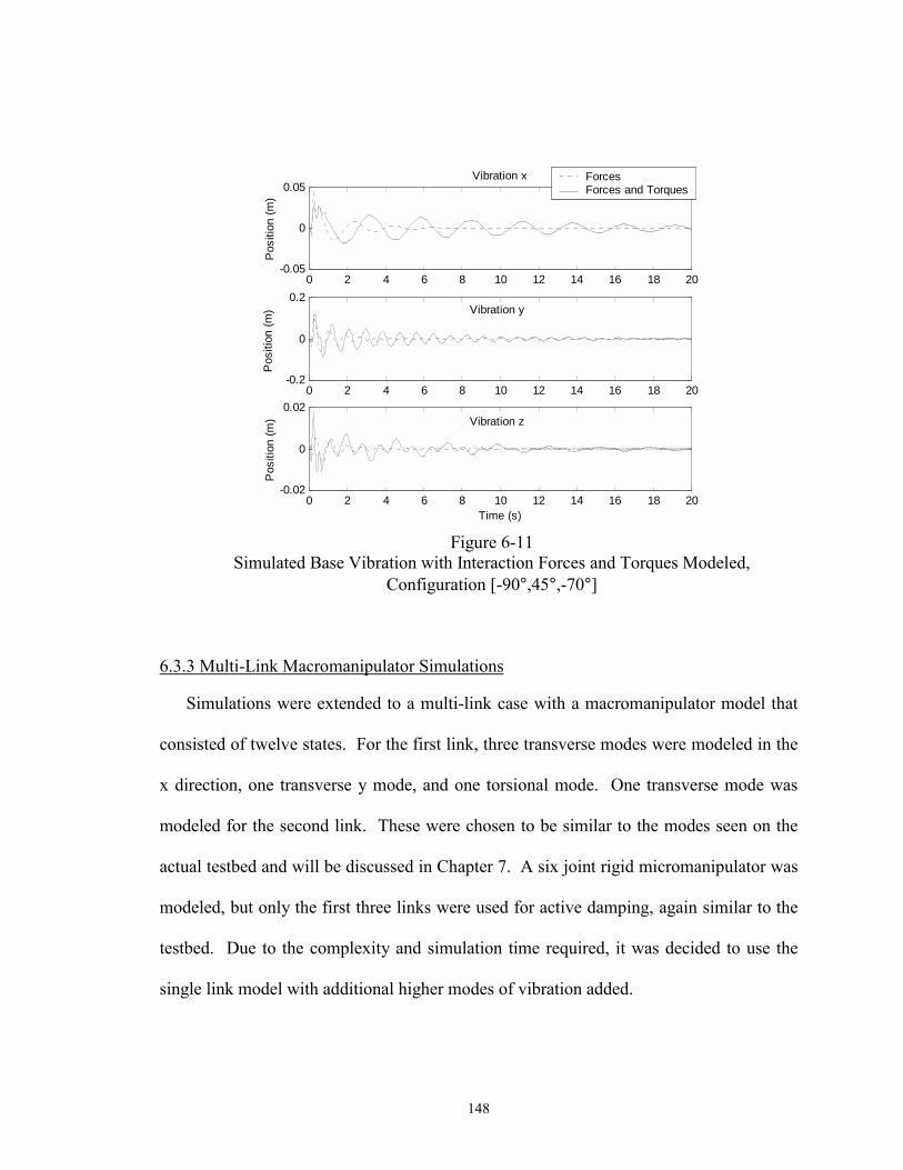
148

0 2 4 6 8 10 12 14 16 18 20-0.05

0

0.05Vibration x

Pos

ition

(m)

0 2 4 6 8 10 12 14 16 18 20-0.2

0

0.2Vibration y

Pos

ition

(m)

0 2 4 6 8 10 12 14 16 18 20-0.02

0

0.02Vibration z

Time (s)

Pos

ition

(m)

Forces Forces and Torques

Figure 6-11

Simulated Base Vibration with Interaction Forces and Torques Modeled, Configuration [-90°,45°,-70°]

6.3.3 Multi-Link Macromanipulator Simulations

Simulations were extended to a multi-link case with a macromanipulator model that

consisted of twelve states. For the first link, three transverse modes were modeled in the

x direction, one transverse y mode, and one torsional mode. One transverse mode was

modeled for the second link. These were chosen to be similar to the modes seen on the

actual testbed and will be discussed in Chapter 7. A six joint rigid micromanipulator was

modeled, but only the first three links were used for active damping, again similar to the

testbed. Due to the complexity and simulation time required, it was decided to use the

single link model with additional higher modes of vibration added.

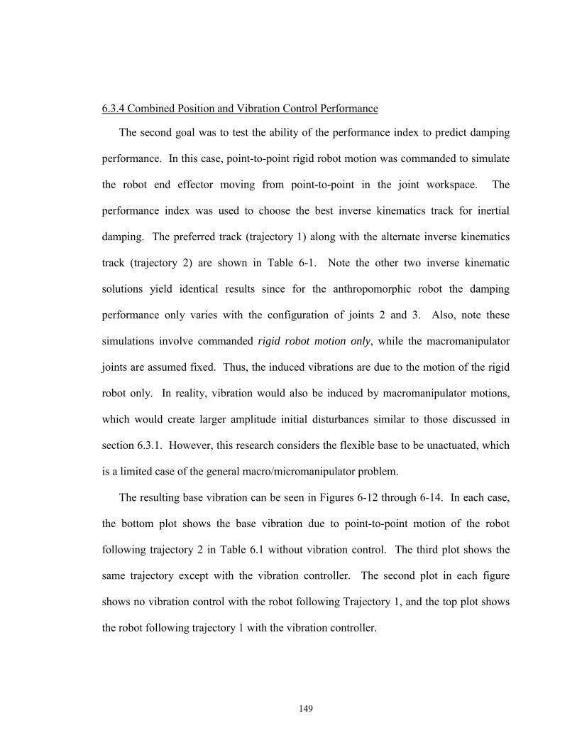
149

6.3.4 Combined Position and Vibration Control Performance

The second goal was to test the ability of the performance index to predict damping

performance. In this case, point-to-point rigid robot motion was commanded to simulate

the robot end effector moving from point-to-point in the joint workspace. The

performance index was used to choose the best inverse kinematics track for inertial

damping. The preferred track (trajectory 1) along with the alternate inverse kinematics

track (trajectory 2) are shown in Table 6-1. Note the other two inverse kinematic

solutions yield identical results since for the anthropomorphic robot the damping

performance only varies with the configuration of joints 2 and 3. Also, note these

simulations involve commanded rigid robot motion only, while the macromanipulator

joints are assumed fixed. Thus, the induced vibrations are due to the motion of the rigid

robot only. In reality, vibration would also be induced by macromanipulator motions,

which would create larger amplitude initial disturbances similar to those discussed in

section 6.3.1. However, this research considers the flexible base to be unactuated, which

is a limited case of the general macro/micromanipulator problem.

The resulting base vibration can be seen in Figures 6-12 through 6-14. In each case,

the bottom plot shows the base vibration due to point-to-point motion of the robot

following trajectory 2 in Table 6.1 without vibration control. The third plot shows the

same trajectory except with the vibration controller. The second plot in each figure

shows no vibration control with the robot following Trajectory 1, and the top plot shows

the robot following trajectory 1 with the vibration controller.

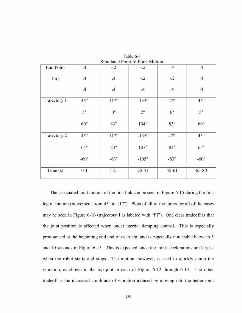
150

Table 6-1 Simulated Point-to-Point Motion

End Point

(m)

.4

.4

.4

-.2

.4

.4

-.2

-.2

.4

.4

-.2

.4

.4

.4

.4

Trajectory 1 45°

5°

60°

117°

0°

83°

-135°

2°

104°

-27°

0°

83°

45°

5°

60°

Trajectory 2 45°

65°

-60°

117°

83°

-83°

-135°

107°

-105°

-27°

83°

-83°

45°

65°

-60°

Time (s) 0-1 5-21 25-41 45-61 65-80

The associated joint motion of the first link can be seen in Figure 6-15 during the first

leg of motion (movement from 45° to 117°). Plots of all of the joints for all of the cases

may be seen in Figure 6-16 (trajectory 1 is labeled with �PI�). One clear tradeoff is that

the joint position is affected when under inertial damping control. This is especially

pronounced at the beginning and end of each leg, and is especially noticeable between 5

and 10 seconds in Figure 6-15. This is expected since the joint accelerations are largest

when the robot starts and stops. The motion, however, is used to quickly damp the

vibration, as shown in the top plot in each of Figure 6-12 through 6-14. The other

tradeoff is the increased amplitude of vibration induced by moving into the better joint

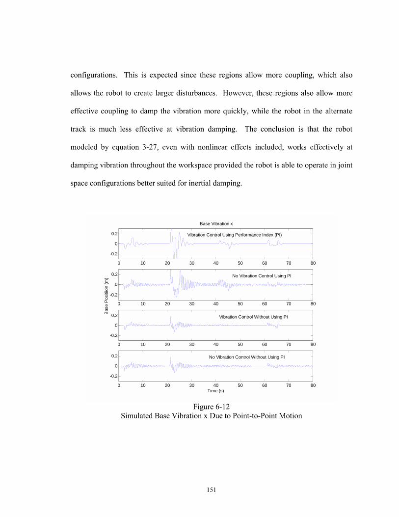
151

configurations. This is expected since these regions allow more coupling, which also

allows the robot to create larger disturbances. However, these regions also allow more

effective coupling to damp the vibration more quickly, while the robot in the alternate

track is much less effective at vibration damping. The conclusion is that the robot

modeled by equation 3-27, even with nonlinear effects included, works effectively at

damping vibration throughout the workspace provided the robot is able to operate in joint

space configurations better suited for inertial damping.

0 10 20 30 40 50 60 70 80 -0.2

0 0.2

Base Vibration x

0 10 20 30 40 50 60 70 80 -0.2

0 0.2

0 10 20 30 40 50 60 70 80 -0.2

0 0.2

Time (s)

0 10 20 30 40 50 60 70 80 -0.2

0 0.2

Bas

e Po

sitii

on (m

)

Vibration Control Using Performance Index (PI)

No Vibration Control Using PI

Vibration Control Without Using PI

No Vibration Control Without Using PI

Figure 6-12

Simulated Base Vibration x Due to Point-to-Point Motion

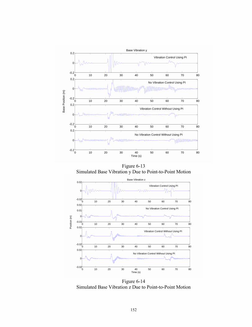
152

0 10 20 30 40 50 60 70 80 -0.2

0

0.2 Base Vibration y

0 10 20 30 40 50 60 70 80 -0.2

0

0.2

0 10 20 30 40 50 60 70 80 -0.2

0

0.2

0 10 20 30 40 50 60 70 80 -0.2

0

0.2

Time (s)

Base

Pos

ition

(m)

Vibration Control Using PI

No Vibration Control Using PI

Vibration Control Without Using PI

No Vibration Control Without Using PI

Figure 6-13

Simulated Base Vibration y Due to Point-to-Point Motion

0 10 20 30 40 50 60 70 80 -0.02

0

0.02 Base Vibration z

0 10 20 30 40 50 60 70 80 -0.01 0

0.01 0.02

Posi

tion

(m)

0 10 20 30 40 50 60 70 80 -0.02

0

0.02 Vibration Control Without Using PI

0 10 20 30 40 50 60 70 80 -0.02

0

0.02

Time (s)

Vibration Control Using PI

No Vibration Control Using PI

No Vibration Control Without Using PI

Figure 6-14

Simulated Base Vibration z Due to Point-to-Point Motion

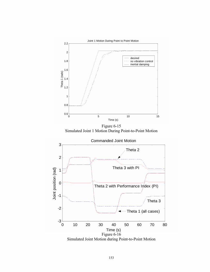
153

0 5 10 150.6

0.8

1

1.2

1.4

1.6

1.8

2

2.2Joint 1 Motion During Point to Point Motion

Time (s)

Thet

a 1

(rads

)desired no vibration controlinertial damping

Figure 6-15

Simulated Joint 1 Motion During Point-to-Point Motion

0 10 20 30 40 50 60 70 80-3

-2

-1

0

1

2

3Commanded Joint Motion

Time (s)

Join

t pos

ition

(rad

)

Theta 2

Theta 3 with PI

Theta 2 with Performance Index (PI)

Theta 3

Theta 1 (all cases)

Figure 6-16

Simulated Joint Motion during Point-to-Point Motion

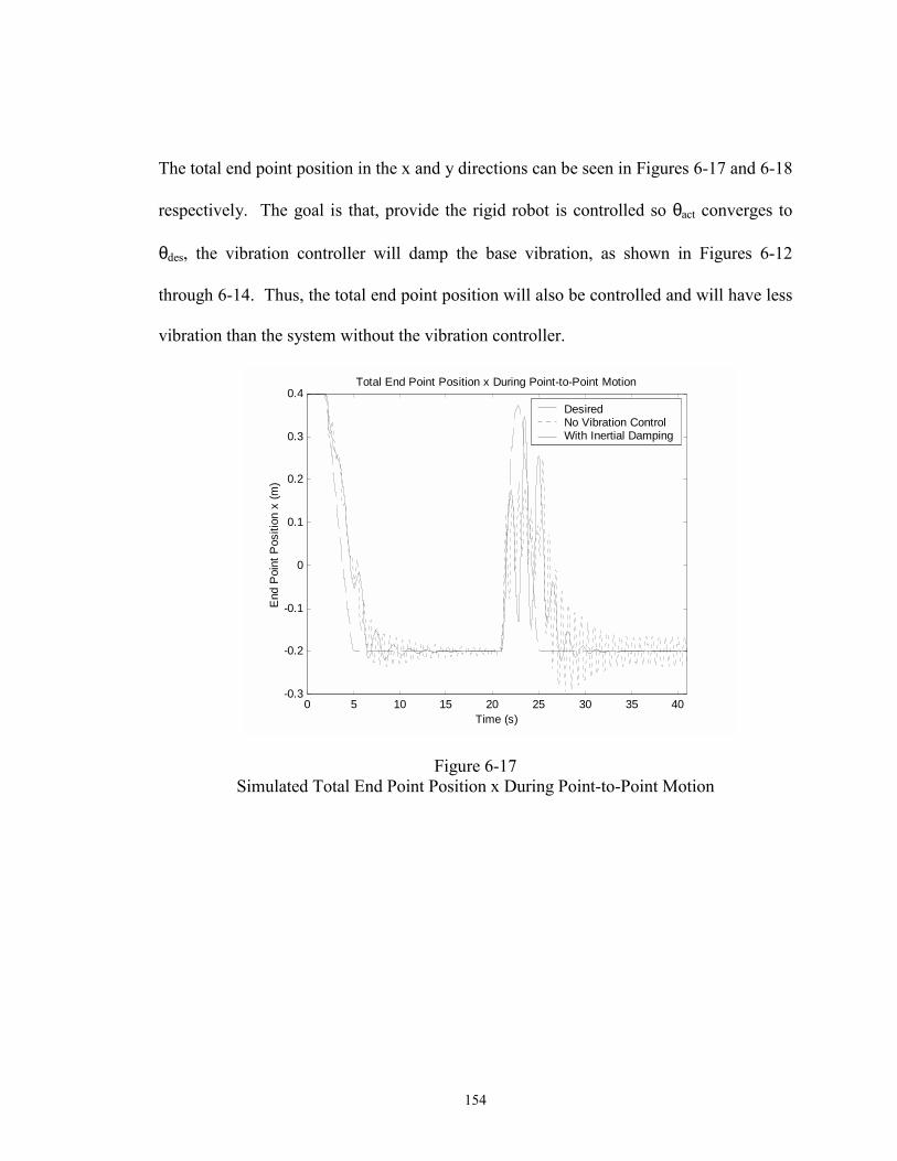
154

The total end point position in the x and y directions can be seen in Figures 6-17 and 6-18

respectively. The goal is that, provide the rigid robot is controlled so θact converges to

θdes, the vibration controller will damp the base vibration, as shown in Figures 6-12

through 6-14. Thus, the total end point position will also be controlled and will have less

vibration than the system without the vibration controller.

0 5 10 15 20 25 30 35 40-0.3

-0.2

-0.1

0

0.1

0.2

0.3

0.4Total End Point Position x During Point-to-Point Motion

Time (s)

End

Poi

nt P

ositi

on x

(m)

Desired No Vibration Control With Inertial Damping

Figure 6-17 Simulated Total End Point Position x During Point-to-Point Motion

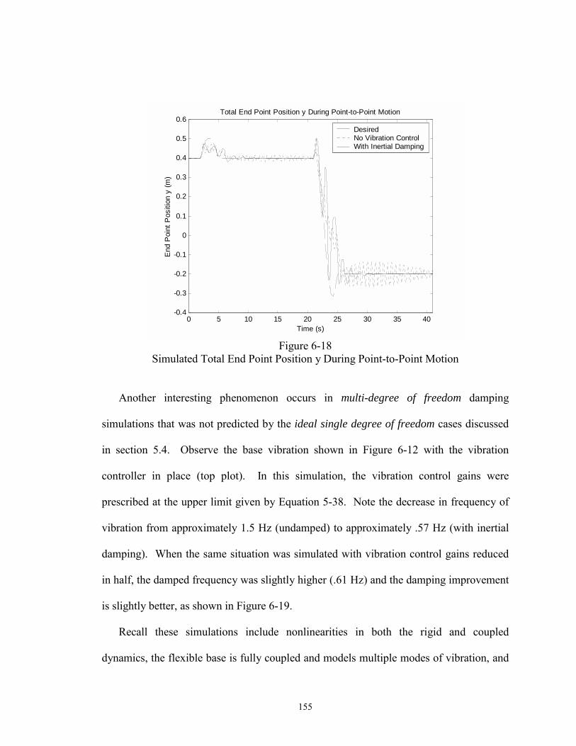
155

0 5 10 15 20 25 30 35 40-0.4

-0.3

-0.2

-0.1

0

0.1

0.2

0.3

0.4

0.5

0.6Total End Point Position y During Point-to-Point Motion

Time (s)

End

Poi

nt P

ositi

on y

(m)

Desired No Vibration Control With Inertial Damping

Figure 6-18

Simulated Total End Point Position y During Point-to-Point Motion

Another interesting phenomenon occurs in multi-degree of freedom damping

simulations that was not predicted by the ideal single degree of freedom cases discussed

in section 5.4. Observe the base vibration shown in Figure 6-12 with the vibration

controller in place (top plot). In this simulation, the vibration control gains were

prescribed at the upper limit given by Equation 5-38. Note the decrease in frequency of

vibration from approximately 1.5 Hz (undamped) to approximately .57 Hz (with inertial

damping). When the same situation was simulated with vibration control gains reduced

in half, the damped frequency was slightly higher (.61 Hz) and the damping improvement

is slightly better, as shown in Figure 6-19.

Recall these simulations include nonlinearities in both the rigid and coupled

dynamics, the flexible base is fully coupled and models multiple modes of vibration, and

156

the simulations are for a three degree of freedom rigid robot. The root locus of the ideal,

linearized case analyzed in Figure 5-10 and shown again below in Figure 6-20, only

approximates the true multi-degree of freedom case. These results could indicate several

things. First, it could indicate that the maximum damping available occurs at a much

lower gain than predicted (case 1). It could also indicate the flexible poles move away

from the jω axis with a steep slope (case 2), which would result in the observed decrease

in frequency of vibration with increasing vibration control gains (case 2). Note Figures

5-4 and 5-9 predicted this behavior could occur.

As noted previously, the rigid robot and vibration controllers need to be designed

carefully to ensure ideal performance predicted by Figure 5-10. When nonlinearities and

other inaccuracies are included, even in simulation, this ideal performance may not occur.

It is likely achievable with the proper modification of the rigid joint controller and/or

lower vibration control gains. Nevertheless, the multi-degree of freedom simulations do

indicate the damping controller can remove overall system energy and improve vibration

performance over the system with no vibration damping.

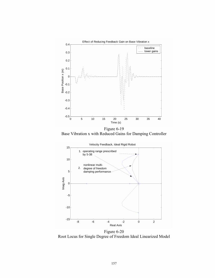
157

0 5 10 15 20 25 30 35 40-0.5

-0.4

-0.3

-0.2

-0.1

0

0.1

0.2

0.3

0.4Effect of Reducing Feedback Gain on Base Vibration x

Time (s)

Bas

e P

ositi

on x

(m)

baseline lower gains

Figure 6-19

Base Vibration x with Reduced Gains for Damping Controller

-8 -6 -4 -2 0 2 -15

-10

-5

0

5

10

15

Real Axis

Imag

Axi

s

Velocity Feedback, Ideal Rigid Robot

operating range prescribedby 5-38

1.

2. nonlinear multi-degree of freedom damping performance

Figure 6-20

Root Locus for Single Degree of Freedom Ideal Linearized Model

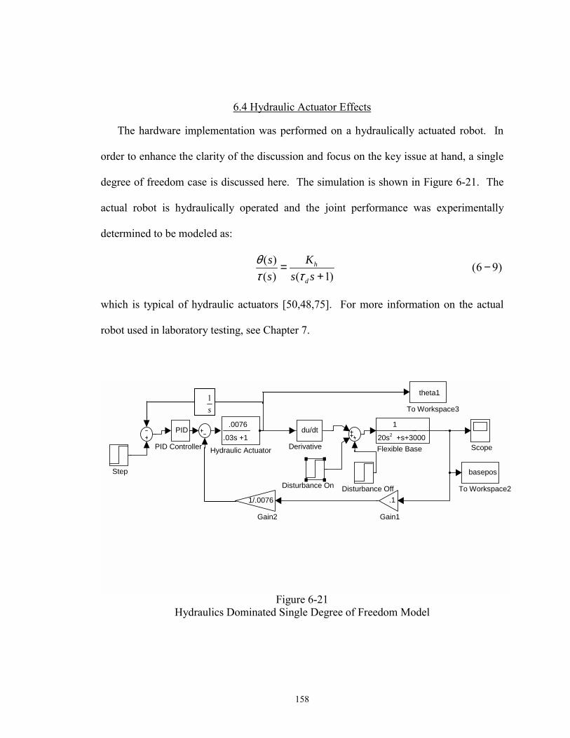
158

6.4 Hydraulic Actuator Effects

The hardware implementation was performed on a hydraulically actuated robot. In

order to enhance the clarity of the discussion and focus on the key issue at hand, a single

degree of freedom case is discussed here. The simulation is shown in Figure 6-21. The

actual robot is hydraulically operated and the joint performance was experimentally

determined to be modeled as:

( ) (6 9)( ) ( 1)

h

d

Kss s s

θτ τ

= −+

which is typical of hydraulic actuators [50,48,75]. For more information on the actual

robot used in laboratory testing, see Chapter 7.

Figure 6-21 Hydraulics Dominated Single Degree of Freedom Model

theta1

To Workspace3

basepos

To Workspace2

Step

Scope

PID

PID Controller

.0076

.03s +1Hydraulic Actuator

1/.0076

Gain2

.1

Gain1

1

20s2 +s+3000 Flexible Base

Disturbance On Disturbance Off

du/dt

Derivative

1s

159

First, the baseline damping performance for the inertially damped and undamped

cases is shown in Figure 6-22 along with the joint motion in Figure 6-23. As these

figures indicate, provided the joint acts as a velocity source the control scheme works

well. Note the joint motion is nearly out of phase with the vibration displacement as

commanded, allowing the vibration energy to be absorbed. Joint 2 was chosen for this

particular test case because it demonstrated the largest amount of phase lag. Next, the

same situation was simulated except with larger τd (as defined in equation 6-9), which

increases phase lag. The resulting base vibration and joint motion is shown in Figure 6-

24. As shown in 6-24, the phasing of the joint motion relative to the vibration has shifted

and no longer effectively removes vibrational energy. As can be seen, the effectiveness

of the scheme decreases, but it is still effective. Provided the actuator can truly be

modeled as a second order system, the phase lag will be no greater than 90° and the

vibration control scheme will still work, although the more phase lag the less effective it

will become.

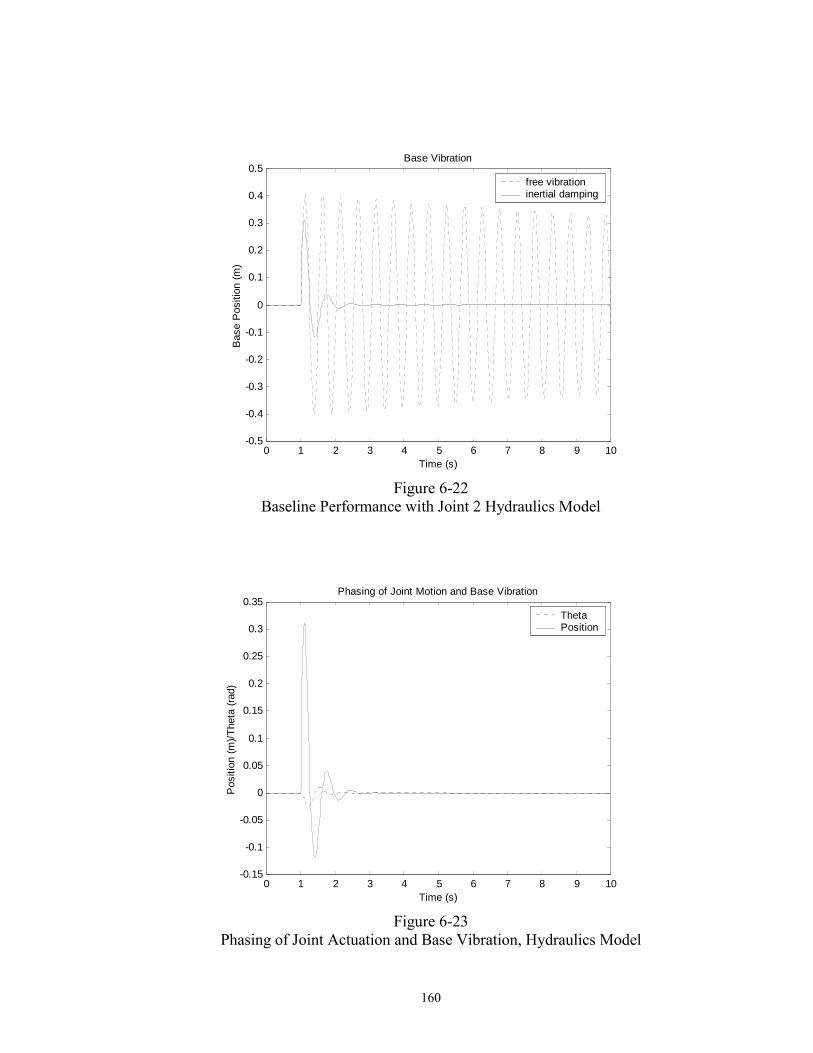
160

0 1 2 3 4 5 6 7 8 9 10-0.5

-0.4

-0.3

-0.2

-0.1

0

0.1

0.2

0.3

0.4

0.5Base Vibration

Time (s)

Bas

e P

ositi

on (m

)

free vibration inertial damping

Figure 6-22

Baseline Performance with Joint 2 Hydraulics Model

0 1 2 3 4 5 6 7 8 9 10-0.15

-0.1

-0.05

0

0.05

0.1

0.15

0.2

0.25

0.3

0.35Phasing of Joint Motion and Base Vibration

Time (s)

Pos

ition

(m)/T

heta

(rad

)

Theta Position

Figure 6-23

Phasing of Joint Actuation and Base Vibration, Hydraulics Model

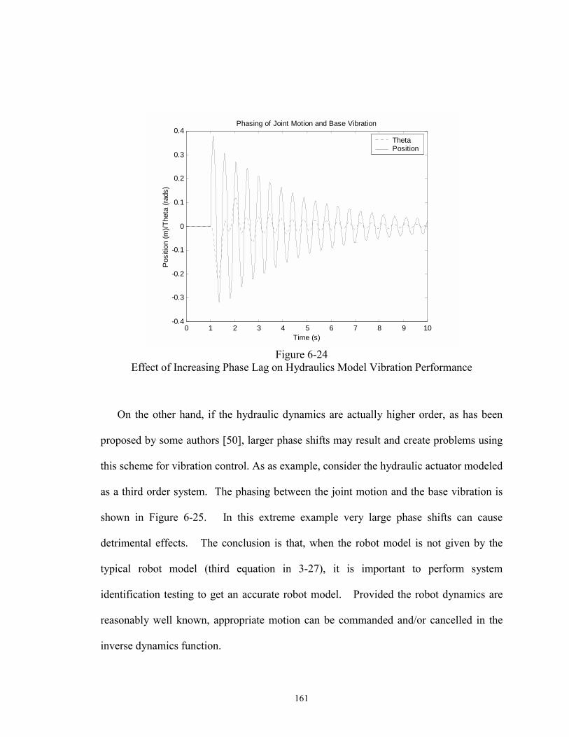
161

0 1 2 3 4 5 6 7 8 9 10-0.4

-0.3

-0.2

-0.1

0

0.1

0.2

0.3

0.4Phasing of Joint Motion and Base Vibration

Time (s)

Pos

ition

(m)/T

heta

(rad

s)

Theta Position

Figure 6-24

Effect of Increasing Phase Lag on Hydraulics Model Vibration Performance

On the other hand, if the hydraulic dynamics are actually higher order, as has been

proposed by some authors [50], larger phase shifts may result and create problems using

this scheme for vibration control. As as example, consider the hydraulic actuator modeled

as a third order system. The phasing between the joint motion and the base vibration is

shown in Figure 6-25. In this extreme example very large phase shifts can cause

detrimental effects. The conclusion is that, when the robot model is not given by the

typical robot model (third equation in 3-27), it is important to perform system

identification testing to get an accurate robot model. Provided the robot dynamics are

reasonably well known, appropriate motion can be commanded and/or cancelled in the

inverse dynamics function.

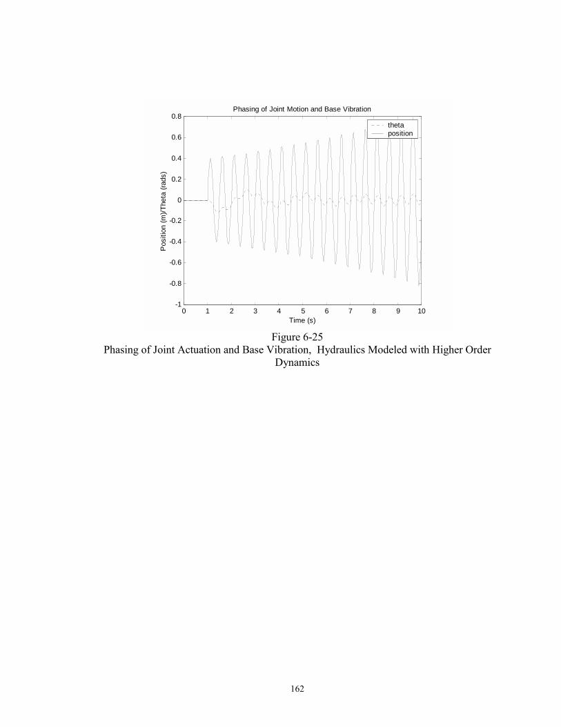
162

0 1 2 3 4 5 6 7 8 9 10-1

-0.8

-0.6

-0.4

-0.2

0

0.2

0.4

0.6

0.8Phasing of Joint Motion and Base Vibration

Time (s)

Pos

ition

(m)/T

heta

(rad

s)

theta position

Figure 6-25

Phasing of Joint Actuation and Base Vibration, Hydraulics Modeled with Higher Order Dynamics

163

CHAPTER VII

EXPERIMENTAL WORK

7.1 Introduction

This chapter describes the experimental testbed and test results. The testbed

consisted of a two flexible link macromanipulator with a six degree of freedom

anthropomorphic/wrist rigid robot mounted to its last link. The experimental work

consisted of two primary areas:

1) Experimental verification of the interaction forces and torques and conclusions

described in Chapter 4. The main area of interest was on the controllable interactions due

to the rigid robot.

2) Implementation of the vibration control scheme on a multi-degree of freedom testbed

This chapter will end with a discussion on issues that arose during hardware

implementation and recommendations for improving the existing testbed.

7.2 Experimental Testbed

A schematic overview of the laboratory setup is shown in Figure 7-1. One of the

common problems with experimental results performed on macro/micromanipulators is

they lack the complexity of real-world applications [10]. For this reason, the testbed was

164

intentionally designed to be as realistic as possible. The testbed was modified from a

single link flexible beam/three degree of freedom micromanipulator, used for research in

[42], to a two flexible link/six degree of freedom micromanipulator. The real-time

control is handled by VxWorks Real Time Control Software, Version 5.2 [85,86]. All of

the control functions that interface with VX Works were written in C [29,43]. The

control is performed using a Motorola 68040 Microprocessor and Acromag AVME D/A,

A/D, and DIO boards for processing of the various signals [44,67].

The rigid robot consists of a hydraulically operated anthropomorphic robot with an

IBM 7565 wrist mounted to its last link [27]. The anthropomorphic robot is operated by

Micro-Precision Textron SS-.5A double vane, SS-.5A single vane, and SS-1A double

vane actuators, while the wrist is operated by similar vane actuators. The servovalves are

Moog series 30 and 31, which operate at a constant maximum current of 15 ma [51,76].

The outgoing voltage signal from the D/A board is first sent through voltage to current

amplifiers before the signal is sent to the valves. US Digital optical encoders are used to

measure the joint position of the first three links of the robot, while potentiometers are

used for the last three joints. Vibration is measured by PCB Accelerometers, one

mounted along each axis (x, y, and z) [57]. During the initial part of the experimental

work, a six axis ATI Delta 9105-T Force/Torque sensor was used to measure interaction

forces and torques at the base of the rigid robot [1].

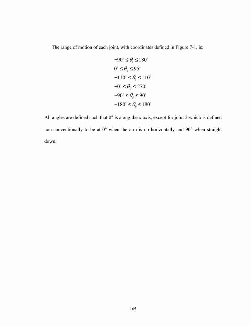
165

The range of motion of each joint, with coordinates defined in Figure 7-1, is:

1

2

3

4

5

6

90 180

0 95

110 110

0 270

90 90

180 180

θθ

θθθθ

− ≤ ≤

≤ ≤

− ≤ ≤

− ≤ ≤

− ≤ ≤

− ≤ ≤

o o

o o

o o

o o

o o

o o

All angles are defined such that 0° is along the x axis, except for joint 2 which is defined

non-conventionally to be at 0° when the arm is up horizontally and 90° when straight

down.

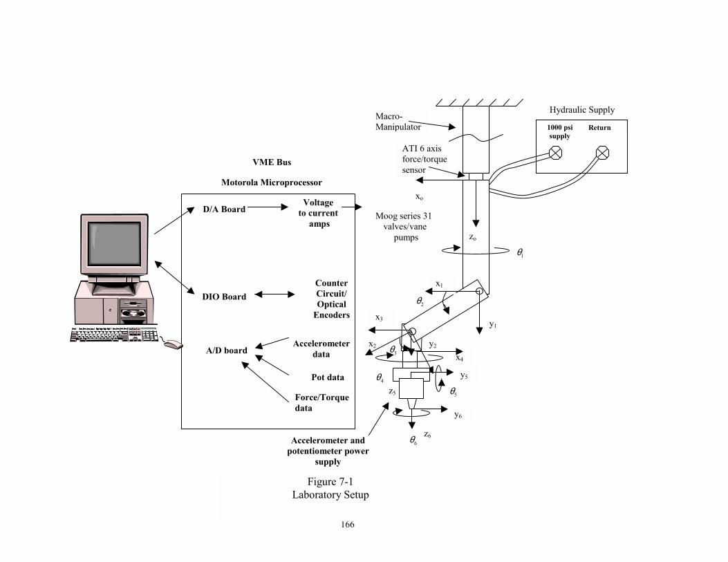
166

Hydraulic Supply

Return

ATI 6 axis force/torque sensor

x4

Accelerometer and potentiometer power

supply

VME Bus

Motorola Microprocessor

A/D board

D/A Board

Pot data

Voltage to current

amps Moog series 31

valves/vane pumps

1000 psi supply

y2 x2

zo

xo

x1

y1 x3

y5

z5

z6

y6

DIO Board Counter Circuit/ Optical

Encoders

Accelerometer data

Force/Torque data

Macro-Manipulator

1θ

2θ

3θ

4θ

5θ

6θ

Figure 7-1 Laboratory Setup

167

7.2.1 Rigid Robot Independent Joint Controllers

The dynamics of the experimental robot are dominated by the hydraulic valves. The

experimental rigid robot is shown in Figure 7-2. Each joint was independently controlled

with a proportional-integral (PI) controller and a dead zone inverse (DZI), as shown in

Figure 7-3. The PI gains were chosen based on the hydraulic valve models, which were

experimentally determined by open loop system identification testing. DZI is a dead-

zone inverse that was designed to compensate for hydraulic actuator dead zone. It is not

the common dead zone inverse as described in [74], but only includes an additional

constant signal output to counter the effects of the valve dead-zone (zero output is offset).

The rigid robot torque equation, or last equation in 3-27, is given by the actuator

specific model. In the case of Moog servovalves, a first order approximation for low

frequency performance was used and is given by [75]:

( ) (7-1)( ) 1d

Q s Ki s sτ

=+

Where: Q=flow rate (cubic inches) i=current input (ma) K=servovalve static flow gain at zero load pressure drop (cubic inches/ma) τd=apparent servovalve time constant (sec)

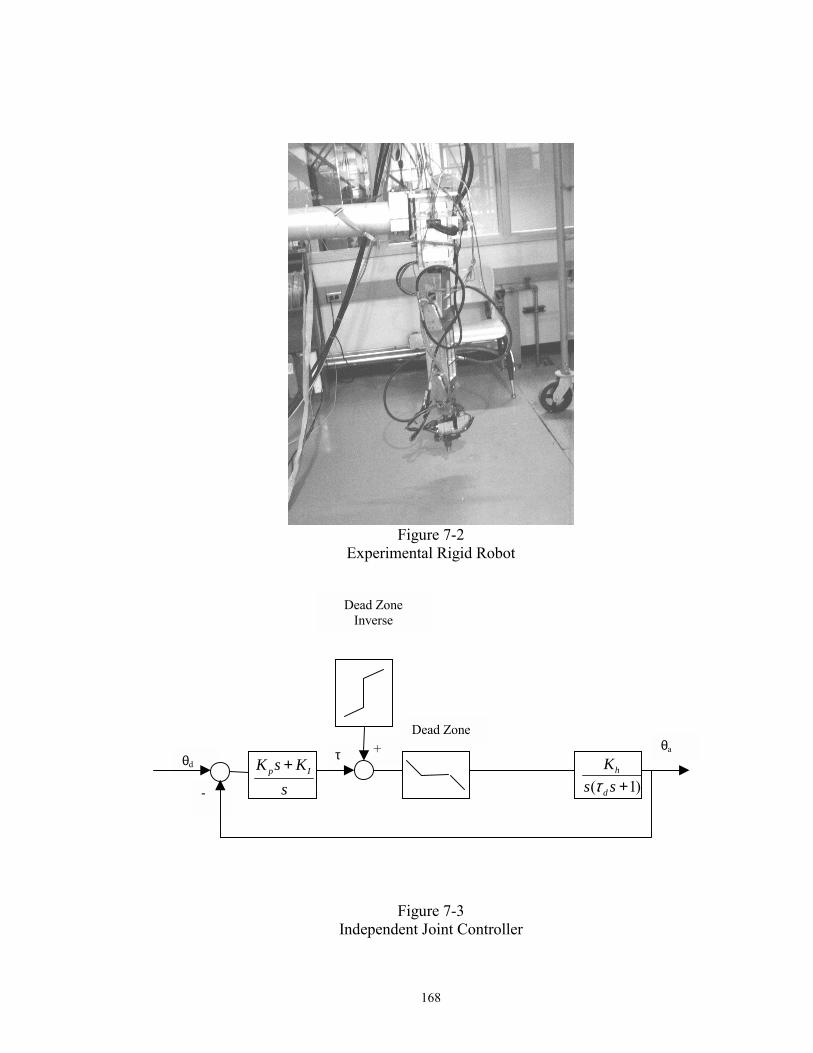
168

Figure 7-2

Experimental Rigid Robot

Figure 7-3

Independent Joint Controller

+

-

τθd

θa

Dead Zone

Dead Zone Inverse

p IK s Ks+

( 1)h

d

Ks sτ +

169

However, the relationship between the commanded computer output, τ, and the resulting

joint motion, θa, was needed. K generally depends upon the rated flow and input current,

while τd depends on the flow capacity of the valve. Since the flow rate is proportional to

robot velocity and current proportional to the D/A output to the robot, the rigid robot

model becomes:

( ) (7-2)( ) ( 1)

h

d

Kss s s

θτ τ

=+

Open loop tests were performed to determine the appropriate modeling constants for each

joint. One representative example may be seen in Figure 7-4, which shows the response

of joint 1 to an output signal of �100, which corresponds to an output voltage of

approximately -.54 volts. These tests were performed over a range of output values

expected for inertial damping control and the results averaged over the range of values.

The resulting model parameters may be seen in Table 7-1.

Table 7-1 Model Parameters for Second Order Approximation of Moog Servovalves

Kh τd Joint 1 -.003459 .00379 Joint 2 -.00076 .03445 Joint 3 -.001775 .017704 Joint 4 .005158 .031648 Joint 5 .00394 .00356 Joint 6 .006 .0248

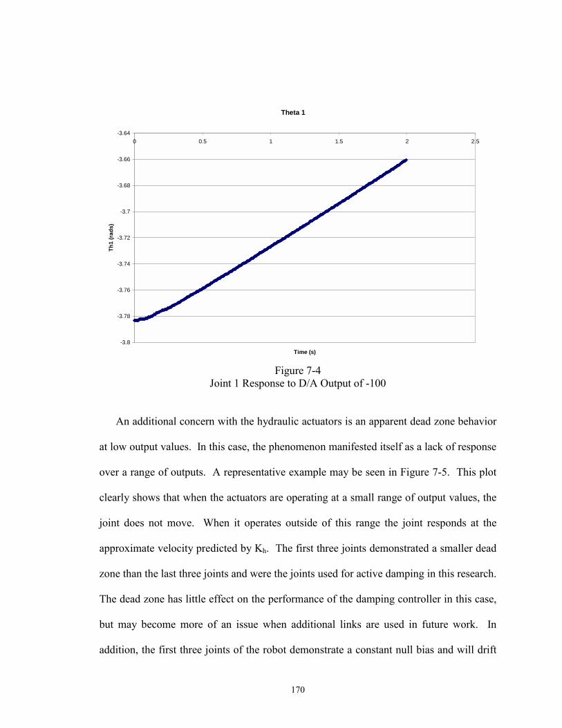
170

Theta 1

-3.8

-3.78

-3.76

-3.74

-3.72

-3.7

-3.68

-3.66

-3.640 0.5 1 1.5 2 2.5

Time (s)

Th1

(rad

s)

Figure 7-4

Joint 1 Response to D/A Output of -100

An additional concern with the hydraulic actuators is an apparent dead zone behavior

at low output values. In this case, the phenomenon manifested itself as a lack of response

over a range of outputs. A representative example may be seen in Figure 7-5. This plot

clearly shows that when the actuators are operating at a small range of output values, the

joint does not move. When it operates outside of this range the joint responds at the

approximate velocity predicted by Kh. The first three joints demonstrated a smaller dead

zone than the last three joints and were the joints used for active damping in this research.

The dead zone has little effect on the performance of the damping controller in this case,

but may become more of an issue when additional links are used in future work. In

addition, the first three joints of the robot demonstrate a constant null bias and will drift

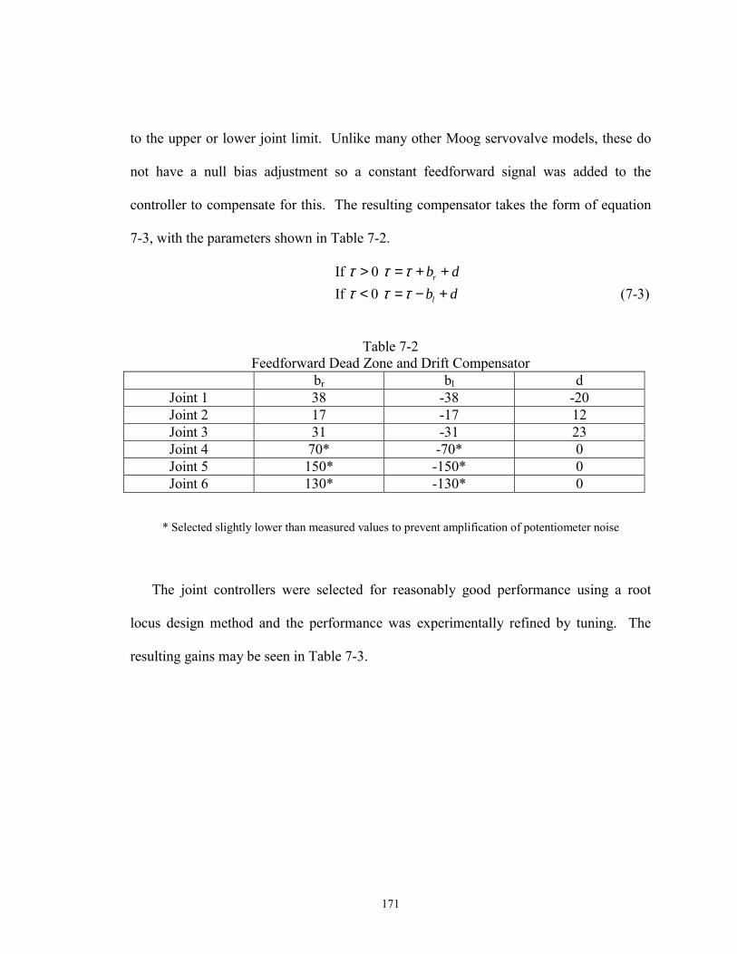
171

to the upper or lower joint limit. Unlike many other Moog servovalve models, these do

not have a null bias adjustment so a constant feedforward signal was added to the

controller to compensate for this. The resulting compensator takes the form of equation

7-3, with the parameters shown in Table 7-2.

If 0 If 0 (7-3)

r

l

b db d

τ τ ττ τ τ> = + +< = − +

Table 7-2

Feedforward Dead Zone and Drift Compensator br bl d

Joint 1 38 -38 -20 Joint 2 17 -17 12 Joint 3 31 -31 23 Joint 4 70* -70* 0 Joint 5 150* -150* 0 Joint 6 130* -130* 0

* Selected slightly lower than measured values to prevent amplification of potentiometer noise

The joint controllers were selected for reasonably good performance using a root

locus design method and the performance was experimentally refined by tuning. The

resulting gains may be seen in Table 7-3.

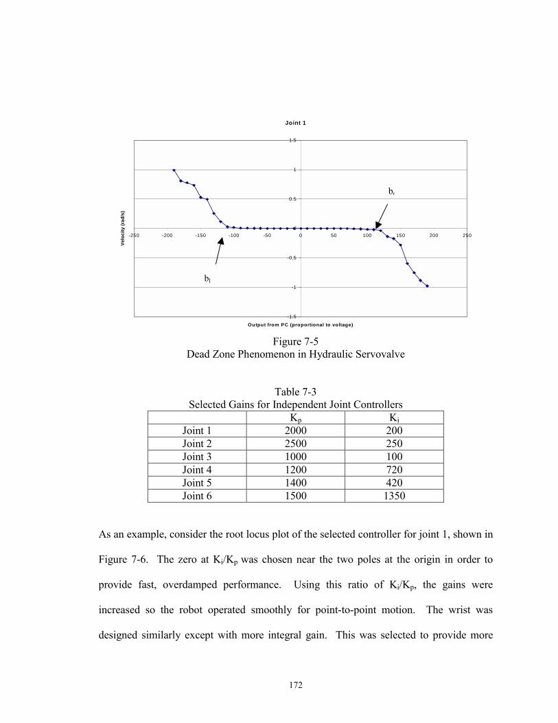
172

Figure 7-5 Dead Zone Phenomenon in Hydraulic Servovalve

Table 7-3 Selected Gains for Independent Joint Controllers

Kp Ki Joint 1 2000 200 Joint 2 2500 250 Joint 3 1000 100 Joint 4 1200 720 Joint 5 1400 420 Joint 6 1500 1350

As an example, consider the root locus plot of the selected controller for joint 1, shown in

Figure 7-6. The zero at Ki/Kp was chosen near the two poles at the origin in order to

provide fast, overdamped performance. Using this ratio of Ki/Kp, the gains were

increased so the robot operated smoothly for point-to-point motion. The wrist was

designed similarly except with more integral gain. This was selected to provide more

Joint 1

-1.5

-1

-0.5

0

0.5

1

1.5

-250 -200 -150 -100 -50 0 50 100 150 200 250

Output from PC (proportional to voltage)

Velo

city

(rad

/s)

bl

br

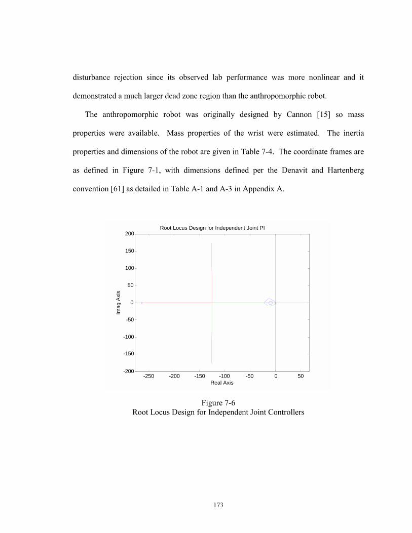
173

disturbance rejection since its observed lab performance was more nonlinear and it

demonstrated a much larger dead zone region than the anthropomorphic robot.

The anthropomorphic robot was originally designed by Cannon [15] so mass

properties were available. Mass properties of the wrist were estimated. The inertia

properties and dimensions of the robot are given in Table 7-4. The coordinate frames are

as defined in Figure 7-1, with dimensions defined per the Denavit and Hartenberg

convention [61] as detailed in Table A-1 and A-3 in Appendix A.

-250 -200 -150 -100 -50 0 50 -200

-150

-100

-50

0

50

100

150

200

Real Axis

Imag

Axi

s

Root Locus Design for Independent Joint PI

Figure 7-6 Root Locus Design for Independent Joint Controllers

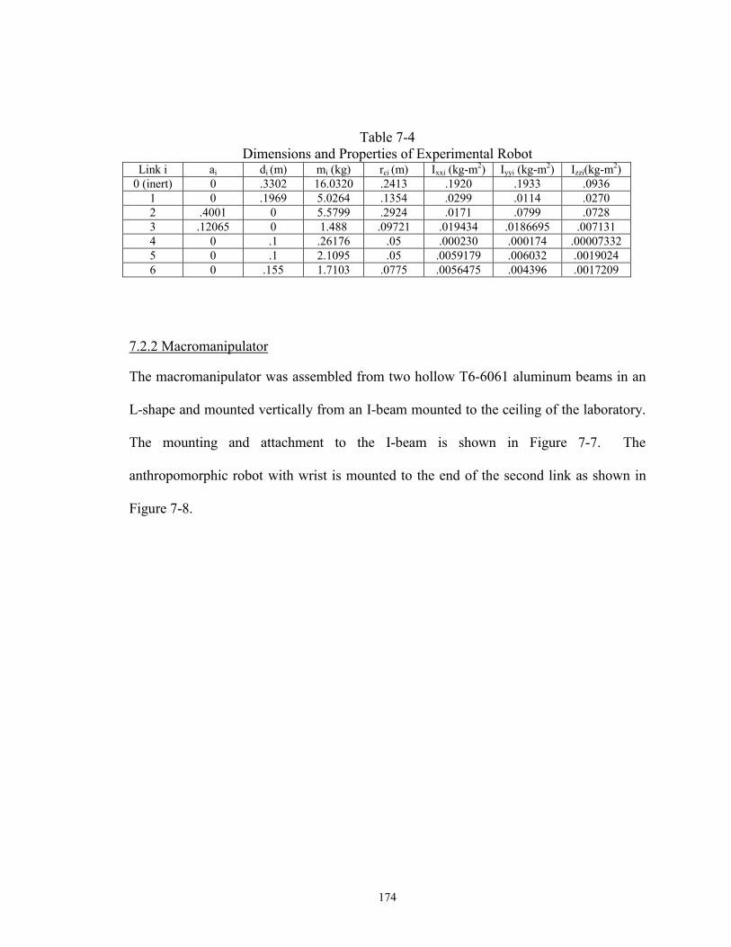
174

Table 7-4 Dimensions and Properties of Experimental Robot

Link i ai di (m) mi (kg) rci (m) Ixxi (kg-m2) Iyyi (kg-m2) Izzi(kg-m2) 0 (inert) 0 .3302 16.0320 .2413 .1920 .1933 .0936

1 0 .1969 5.0264 .1354 .0299 .0114 .0270 2 .4001 0 5.5799 .2924 .0171 .0799 .0728 3 .12065 0 1.488 .09721 .019434 .0186695 .007131 4 0 .1 .26176 .05 .000230 .000174 .00007332 5 0 .1 2.1095 .05 .0059179 .006032 .0019024 6 0 .155 1.7103 .0775 .0056475 .004396 .0017209

7.2.2 Macromanipulator

The macromanipulator was assembled from two hollow T6-6061 aluminum beams in an

L-shape and mounted vertically from an I-beam mounted to the ceiling of the laboratory.

The mounting and attachment to the I-beam is shown in Figure 7-7. The

anthropomorphic robot with wrist is mounted to the end of the second link as shown in

Figure 7-8.

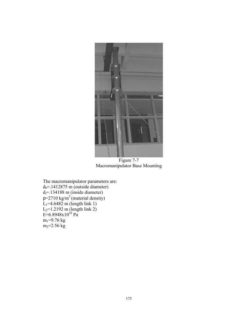
175

Figure 7-7

Macromanipulator Base Mounting

The macromanipulator parameters are: d0=.1412875 m (outside diameter) di=.134188 m (inside diameter) ρ=2710 kg/m3 (material density) L1=4.6482 m (length link 1) L2=1.2192 m (length link 2) E=6.8948x1010 Pa m1=9.76 kg m2=2.56 kg

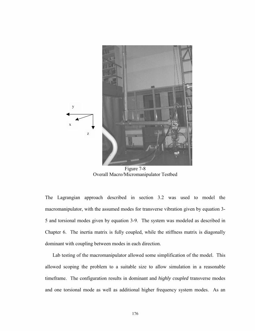
176

Figure 7-8 Overall Macro/Micromanipulator Testbed

The Lagrangian approach described in section 3.2 was used to model the

macromanipulator, with the assumed modes for transverse vibration given by equation 3-

5 and torsional modes given by equation 3-9. The system was modeled as described in

Chapter 6. The inertia matrix is fully coupled, while the stiffness matrix is diagonally

dominant with coupling between modes in each direction.

Lab testing of the macromanipulator allowed some simplification of the model. This

allowed scoping the problem to a suitable size to allow simulation in a reasonable

timeframe. The configuration results in dominant and highly coupled transverse modes

and one torsional mode as well as additional higher frequency system modes. As an

x

y

z

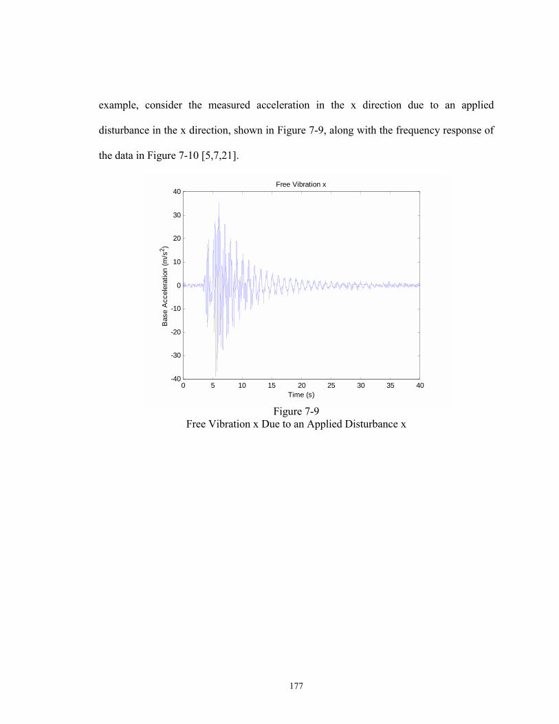
177

example, consider the measured acceleration in the x direction due to an applied

disturbance in the x direction, shown in Figure 7-9, along with the frequency response of

the data in Figure 7-10 [5,7,21].

0 5 10 15 20 25 30 35 40-40

-30

-20

-10

0

10

20

30

40Free Vibration x

Time (s)

Bas

e A

ccel

erat

ion

(m/s

2 )

Figure 7-9

Free Vibration x Due to an Applied Disturbance x

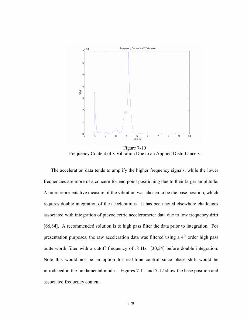
178

0 1 2 3 4 5 6 7 8 9 10 0

1

2

3

4

5

6

7 x 10 4 Frequency Concent of X Vibration

Time (s)

|X(k

)|

Figure 7-10

Frequency Content of x Vibration Due to an Applied Disturbance x

The acceleration data tends to amplify the higher frequency signals, while the lower

frequencies are more of a concern for end point positioning due to their larger amplitude.

A more representative measure of the vibration was chosen to be the base position, which

requires double integration of the accelerations. It has been noted elsewhere challenges

associated with integration of piezoelectric accelerometer data due to low frequency drift

[66,84]. A recommended solution is to high pass filter the data prior to integration. For

presentation purposes, the raw acceleration data was filtered using a 4th order high pass

butterworth filter with a cutoff frequency of .8 Hz [30,54] before double integration.

Note this would not be an option for real-time control since phase shift would be

introduced in the fundamental modes. Figures 7-11 and 7-12 show the base position and

associated frequency content.

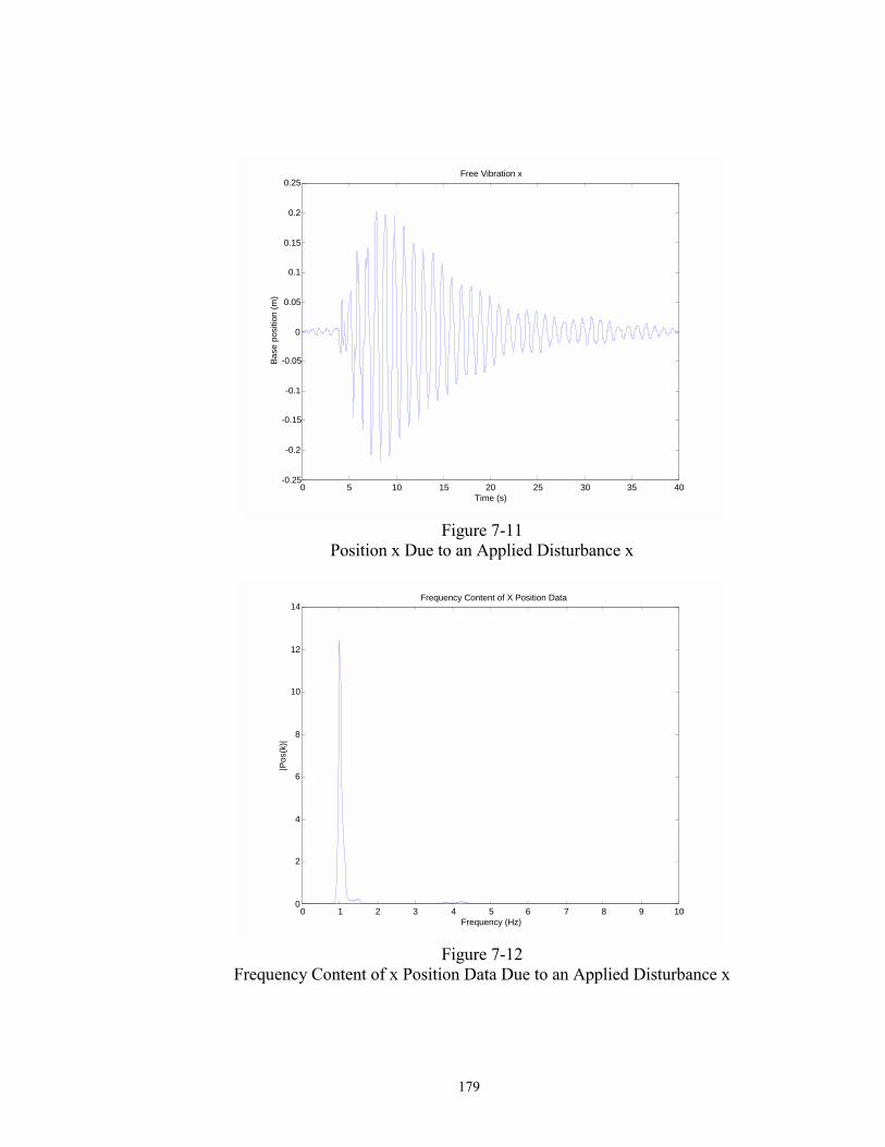
179

0 5 10 15 20 25 30 35 40 -0.25

-0.2

-0.15

-0.1

-0.05

0

0.05

0.1

0.15

0.2

0.25 Free Vibration x

Time (s)

Base

pos

ition

(m)

Figure 7-11

Position x Due to an Applied Disturbance x

0 1 2 3 4 5 6 7 8 9 10 0

2

4

6

8

10

12

14 Frequency Content of X Position Data

Frequency (Hz)

|Pos

(k)|

Figure 7-12

Frequency Content of x Position Data Due to an Applied Disturbance x

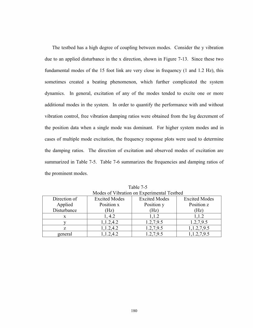
180

The testbed has a high degree of coupling between modes. Consider the y vibration

due to an applied disturbance in the x direction, shown in Figure 7-13. Since these two

fundamental modes of the 15 foot link are very close in frequency (1 and 1.2 Hz), this

sometimes created a beating phenomenon, which further complicated the system

dynamics. In general, excitation of any of the modes tended to excite one or more

additional modes in the system. In order to quantify the performance with and without

vibration control, free vibration damping ratios were obtained from the log decrement of

the position data when a single mode was dominant. For higher system modes and in

cases of multiple mode excitation, the frequency response plots were used to determine

the damping ratios. The direction of excitation and observed modes of excitation are

summarized in Table 7-5. Table 7-6 summarizes the frequencies and damping ratios of

the prominent modes.

Table 7-5 Modes of Vibration on Experimental Testbed

Direction of Applied

Disturbance

Excited Modes Position x

(Hz)

Excited Modes Position y

(Hz)

Excited Modes Position z

(Hz) x 1, 4.2 1,1.2 1,1.2 y 1,1.2,4.2 1.2,7,9.5 1.2,7,9.5 z 1,1.2,4.2 1.2,7,9.5 1,1.2,7,9.5

general 1,1.2,4.2 1.2,7,9.5 1,1.2,7,9.5

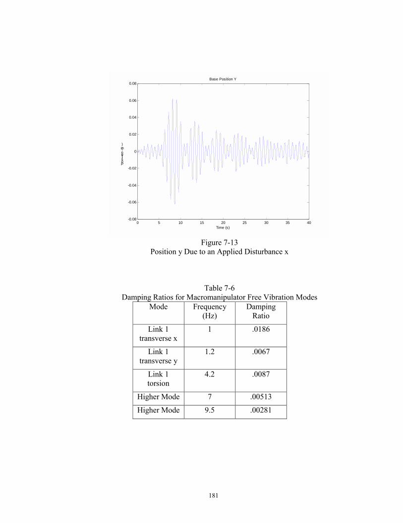
181

0 5 10 15 20 25 30 35 40-0.08

-0.06

-0.04

-0.02

0

0.02

0.04

0.06

0.08Base Position Y

Time (s)

Position (m)

Figure 7-13

Position y Due to an Applied Disturbance x

Table 7-6

Damping Ratios for Macromanipulator Free Vibration Modes Mode Frequency

(Hz) Damping

Ratio

Link 1 transverse x

1 .0186

Link 1 transverse y

1.2 .0067

Link 1 torsion

4.2 .0087

Higher Mode 7 .00513

Higher Mode 9.5 .00281

182

7.3 Interaction Forces and Torques

The first part of the experimental work was intended to verify the method used to

predict the interaction forces and torques and verify work discussed in Chapter 4. Recall

the controllable interactions are given by:

0 0 0 0

( ) ( , ) ( ) ( , , , )

( ) ( , ) ( ) ( , , , ) (7-4)IF f f i j f fc

IF i j c

B N C N

B N C Nτ τ τ τ

= + + +

= + + +

F θ θ θ θ θ θ q q q θ θ

τ θ θ θ θ θ θ q q q θ θ

&& & & &&& &

&& & & &&& &

The directly controllable interactions that were the subject of Chapter 4 are given by

the first two terms in each equation. However, the actual interaction forces and torques

are governed by all of the effects, including those due to the motion of the

macromanipulator. In order to isolate the effects due to the micromanipulator, the base of

the macromanipulator was braced as shown in Figure 7-14. An ATI six-axis force/torque

sensor [1] was mounted between the micromanipulator and the base of the

macromanipulator. Input signals were sent to the rigid robot similar to the motion

expected during active inertial damping, where the motion is harmonic and given by the

last equation 5-12.

7.3.1 Single Degree of Freedom Interaction Forces and Torques

The first goal of this work was to determine if the relationship given by equations

4-4 and 4-8, governing the inertia interaction forces and torques, provide a reasonable

approximation of the dominant interactions. Masses and dimensions of the rigid robot

were estimated as given in Table 7-4. In addition to proving the validity of the

183

relationship for the interactions, it also provided an opportunity to obtain mass property

updates. The first part of this work involved actuating each joint independently, with

constant amplitude sine inputs at 1 and 2 Hz, approximately the lowest natural

frequencies of interest on the tested. It was expected that this would create dominant

inertia forces and torques since:

2

max

2 2

max

20 * cos(2* *1 )180

14 /

5 / (7-5)

t

rad s

rad s

πθ π

θ

θ

=

≈

≈

o

&&

&

An example of the predicted and measured interaction forces and torques due to joint one

can be seen in Figures 7-15 and 7-16, respectively, in a configuration of [-90°, 45°, 45°].

This configuration was chosen because it is near the singularity region, as predicted in

Figure 4-5, but not near enough that it should affect the ability of the robot to create

effective interactions. Thus this configuration would be representative of performance

throughout most of the usable workspace (performance would be better than this in most

locations). The nonlinear force effects are included in Figure 7-15 for magnitude

comparison purposes.

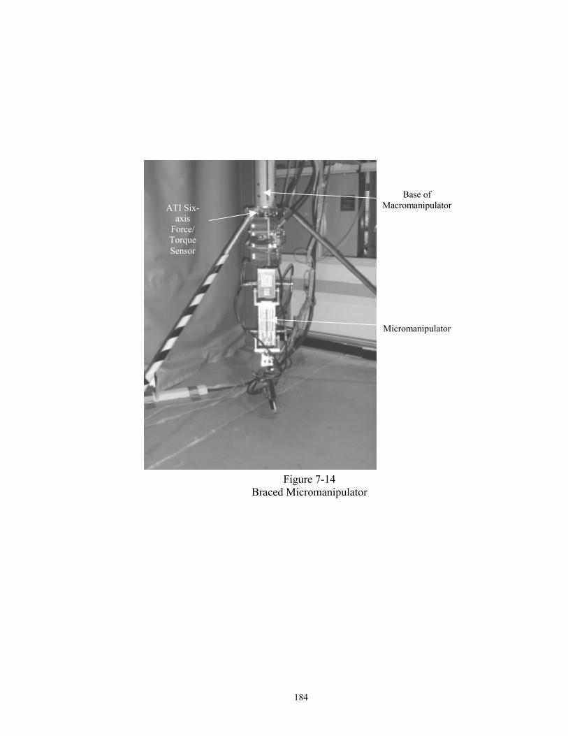
184

Figure 7-14 Braced Micromanipulator

ATI Six-axis

Force/ Torque Sensor

Base of Macromanipulator

Micromanipulator

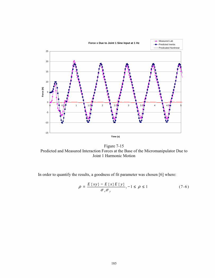
185

Force x Due to Joint 1 Sine Input at 1 Hz

-15

-10

-5

0

5

10

15

20

25

0 0.5 1 1.5 2 2.5 3 3.5 4 4.5 5

Time (s)

Forc

e (N

)Measured LabPredicted InertiaPredicated Nonlinear

Figure 7-15

Predicted and Measured Interaction Forces at the Base of the Micromanipulator Due to Joint 1 Harmonic Motion

In order to quantify the results, a goodness of fit parameter was chosen [6] where:

{ } { } { } , 1 1 (7 -6 )x y

E xy E x E yρ ρσ σ−= − ≤ ≤

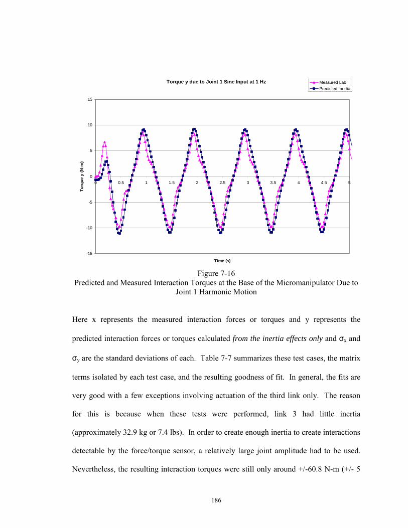
186

Torque y due to Joint 1 Sine Input at 1 Hz

-15

-10

-5

0

5

10

15

0 0.5 1 1.5 2 2.5 3 3.5 4 4.5 5

Time (s)

Torq

ue y

(N-m

)Measured LabPredicted Inertia

Figure 7-16 Predicted and Measured Interaction Torques at the Base of the Micromanipulator Due to

Joint 1 Harmonic Motion

Here x represents the measured interaction forces or torques and y represents the

predicted interaction forces or torques calculated from the inertia effects only and σx and

σy are the standard deviations of each. Table 7-7 summarizes these test cases, the matrix

terms isolated by each test case, and the resulting goodness of fit. In general, the fits are

very good with a few exceptions involving actuation of the third link only. The reason

for this is because when these tests were performed, link 3 had little inertia

(approximately 32.9 kg or 7.4 lbs). In order to create enough inertia to create interactions

detectable by the force/torque sensor, a relatively large joint amplitude had to be used.

Nevertheless, the resulting interaction torques were still only around +/-60.8 N-m (+/- 5

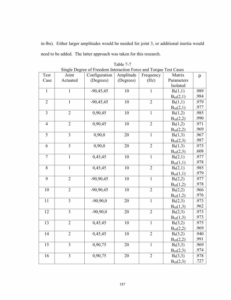
187

in-lbs). Either larger amplitudes would be needed for joint 3, or additional inertia would

need to be added. The latter approach was taken for this research.

Table 7-7 Single Degree of Freedom Interaction Force and Torque Test Cases

Test Case

Joint Actuated

Configuration (Degrees)

Amplitude (Degrees)

Frequency (Hz)

Matrix Parameters

Isolated

ρ

1 1 -90,45,45 10 1 Bf(1,1) Bτ0(2,1)

.989

.984 2 1 -90,45,45 10 2 Bf(1,1)

Bτ0(2,1) .979 .977

3 2 0,90,45 10 1 Bf(1,2) Bτ0(2,2)

.985

.990 4 2 0,90,45 10 2 Bf(1,2)

Bτ0(2,2) .971 .969

5 3 0,90,0 20 1 Bf(1,3) Bτ0(2,3)

.967

.987 6 3 0,90,0 20 2 Bf(1,3)

Bτ0(2,3) .973 .608

7 1 0,45,45 10 1 Bf(2,1) Bτ0(1,1)

.977

.978 8 1 0,45,45 10 2 Bf(2,1)

Bτ0(1,1) .985 .979

9 2 -90,90,45 10 1 Bf(2,2) Bτ0(1,2)

.977

.978 10 2 -90,90,45 10 2 Bf(2,2)

Bτ0(1,2) .966 .976

11 3 -90,90,0 20 1 Bf(2,3) Bτ0(1,3)

.973

.962 12 3 -90,90,0 20 2 Bf(2,3)

Bτ0(1,3) .973 .973

13 2 0,45,45 10 1 Bf(3,2) Bτ0(2,2)

.975

.969 14 2 0,45,45 10 2 Bf(3,2)

Bτ0(2,2) .940 .991

15 3 0,90,75 20 1 Bf(3,3) Bτ0(2,3)

.969

.974 16 3 0,90,75 20 2 Bf(3,3)

Bτ0(2,3) .978 .727

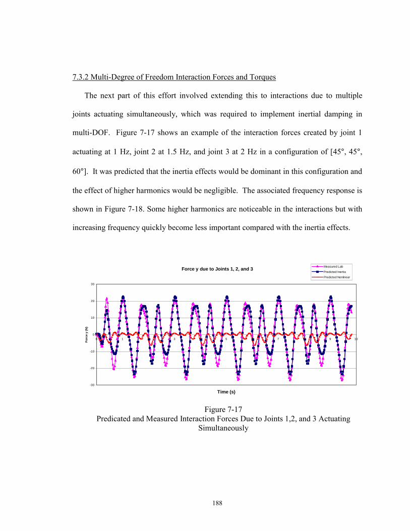
188

7.3.2 Multi-Degree of Freedom Interaction Forces and Torques The next part of this effort involved extending this to interactions due to multiple

joints actuating simultaneously, which was required to implement inertial damping in

multi-DOF. Figure 7-17 shows an example of the interaction forces created by joint 1

actuating at 1 Hz, joint 2 at 1.5 Hz, and joint 3 at 2 Hz in a configuration of [45°, 45°,

60°]. It was predicted that the inertia effects would be dominant in this configuration and

the effect of higher harmonics would be negligible. The associated frequency response is

shown in Figure 7-18. Some higher harmonics are noticeable in the interactions but with

increasing frequency quickly become less important compared with the inertia effects.

Force y due to Joints 1, 2, and 3

-30

-20

-10

0

10

20

30

0 1 2 3 4 5 6 7 8 9 10

Time (s)

Forc

e y

(N)

Measured Lab

Predicted Inertia

Predicted Nonlinear

Figure 7-17

Predicated and Measured Interaction Forces Due to Joints 1,2, and 3 Actuating Simultaneously

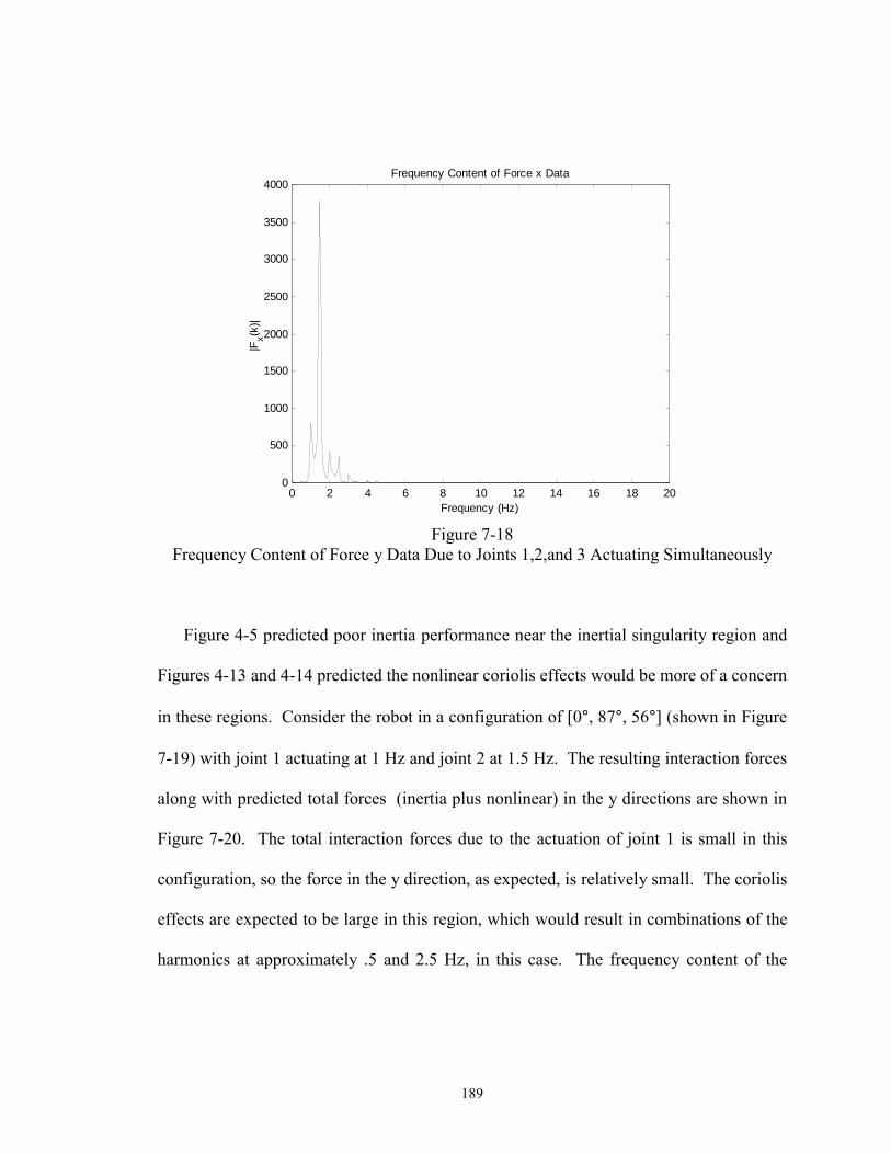
189

0 2 4 6 8 10 12 14 16 18 200

500

1000

1500

2000

2500

3000

3500

4000Frequency Content of Force x Data

Frequency (Hz)

|Fx(k

)|

Figure 7-18

Frequency Content of Force y Data Due to Joints 1,2,and 3 Actuating Simultaneously

Figure 4-5 predicted poor inertia performance near the inertial singularity region and

Figures 4-13 and 4-14 predicted the nonlinear coriolis effects would be more of a concern

in these regions. Consider the robot in a configuration of [0°, 87°, 56°] (shown in Figure

7-19) with joint 1 actuating at 1 Hz and joint 2 at 1.5 Hz. The resulting interaction forces

along with predicted total forces (inertia plus nonlinear) in the y directions are shown in

Figure 7-20. The total interaction forces due to the actuation of joint 1 is small in this

configuration, so the force in the y direction, as expected, is relatively small. The coriolis

effects are expected to be large in this region, which would result in combinations of the

harmonics at approximately .5 and 2.5 Hz, in this case. The frequency content of the

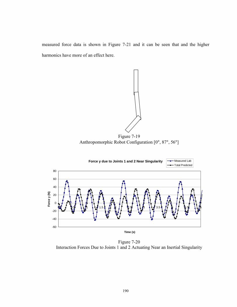
190

measured force data is shown in Figure 7-21 and it can be seen that and the higher

harmonics have more of an effect here.

Figure 7-19 Anthropomorphic Robot Configuration [0°, 87°, 56°]

Force y due to Joints 1 and 2 Near Singularity

-60

-40

-20

0

20

40

60

80

0 0.5 1 1.5 2 2.5 3 3.5 4 4.5 5

Time (s)

Forc

e y

(N)

Measured LabTotal Predicted

Figure 7-20

Interaction Forces Due to Joints 1 and 2 Actuating Near an Inertial Singularity

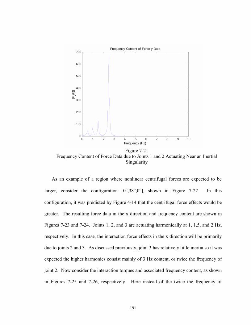
191

0 1 2 3 4 5 6 7 8 9 100

100

200

300

400

500

600

700Frequency Content of Force y Data

Frequency (Hz)

|Fy(k

)|

Figure 7-21

Frequency Content of Force Data due to Joints 1 and 2 Actuating Near an Inertial Singularity

As an example of a region where nonlinear centrifugal forces are expected to be

larger, consider the configuration [0°,38°,0°], shown in Figure 7-22. In this

configuration, it was predicted by Figure 4-14 that the centrifugal force effects would be

greater. The resulting force data in the x direction and frequency content are shown in

Figures 7-23 and 7-24. Joints 1, 2, and 3 are actuating harmonically at 1, 1.5, and 2 Hz,

respectively. In this case, the interaction force effects in the x direction will be primarily

due to joints 2 and 3. As discussed previously, joint 3 has relatively little inertia so it was

expected the higher harmonics consist mainly of 3 Hz content, or twice the frequency of

joint 2. Now consider the interaction torques and associated frequency content, as shown

in Figures 7-25 and 7-26, respectively. Here instead of the twice the frequency of

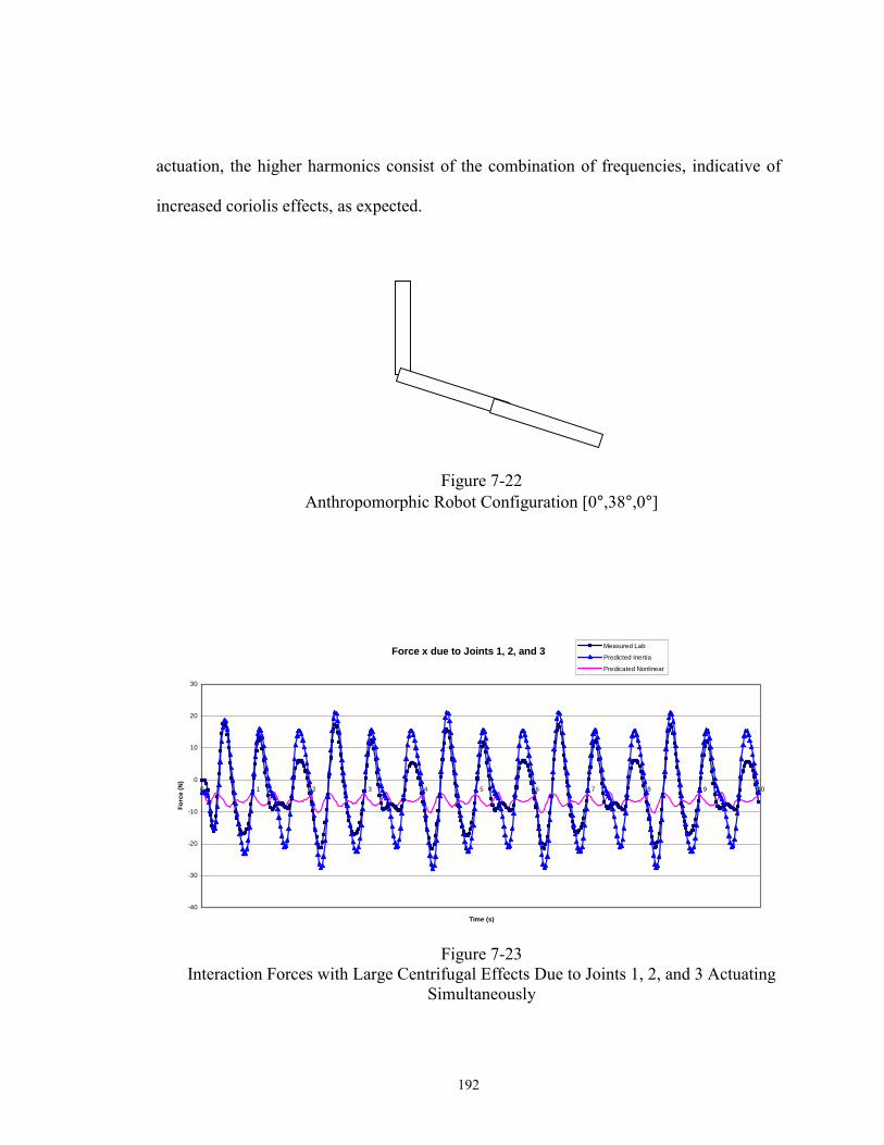
192

actuation, the higher harmonics consist of the combination of frequencies, indicative of

increased coriolis effects, as expected.

Figure 7-22 Anthropomorphic Robot Configuration [0°,38°,0°]

Force x due to Joints 1, 2, and 3

-40

-30

-20

-10

0

10

20

30

0 1 2 3 4 5 6 7 8 9 10

Time (s)

Forc

e (N

)

Measured Lab

Predicted Inertia

Predicated Nonlinear

Figure 7-23

Interaction Forces with Large Centrifugal Effects Due to Joints 1, 2, and 3 Actuating Simultaneously

193

0 1 2 3 4 5 6 7 8 9 100

0.5

1

1.5

2

2.5

3

3.5

4

4.5

5x 104 Frequency Content of Force x Data

Time (s)

|Fx(k

)|

Figure 7-24

Frequency Content of Force x data with Large Centrifugal Effects

Torque x due to Joints 1, 2, and 3

-20

-15

-10

-5

0

5

10

15

20

0 0.5 1 1.5 2 2.5 3 3.5 4 4.5 5

Time (s)

Torq

ue (N

-m)

Measured Lab

Predicted Inertia

Figure 7-25

Interaction Torques due to Joints 1, 2, and 3 in Configuration (0°,38°,0°)

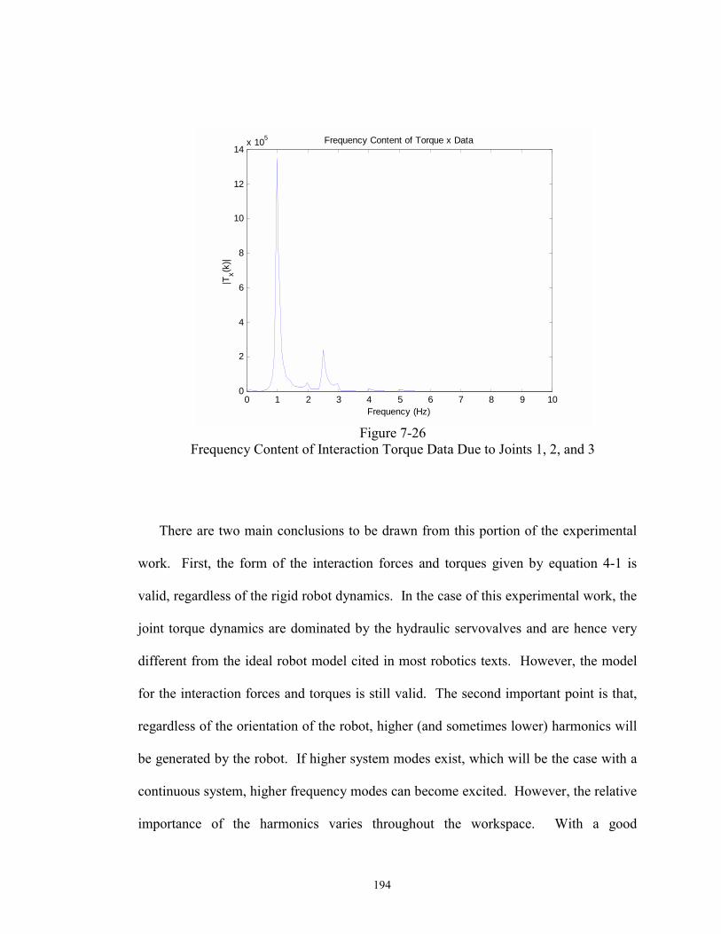
194

0 1 2 3 4 5 6 7 8 9 100

2

4

6

8

10

12

14x 105 Frequency Content of Torque x Data

Frequency (Hz)

|Tx(k

)|

Figure 7-26

Frequency Content of Interaction Torque Data Due to Joints 1, 2, and 3

There are two main conclusions to be drawn from this portion of the experimental

work. First, the form of the interaction forces and torques given by equation 4-1 is

valid, regardless of the rigid robot dynamics. In the case of this experimental work, the

joint torque dynamics are dominated by the hydraulic servovalves and are hence very

different from the ideal robot model cited in most robotics texts. However, the model

for the interaction forces and torques is still valid. The second important point is that,

regardless of the orientation of the robot, higher (and sometimes lower) harmonics will

be generated by the robot. If higher system modes exist, which will be the case with a

continuous system, higher frequency modes can become excited. However, the relative

importance of the harmonics varies throughout the workspace. With a good

195

understanding of these issues, either these regions can be avoided or the control gains

selected to ensure overall energy removal from the system. Note this part of the work

has assumed constant joint amplitudes, and the ratio of the inertia to nonlinear effects

will improve as the vibration is reduced. The next step was to proceed forward with

implementation of the vibration controller described in Chapter 5.

7.4 Multi-Degree of Freedom Vibration Damping

The final goal of this research was to extend the inertial damping control scheme to

multiple degrees of freedom. This is a challenging extension from previous work at

Georgia Tech for two main reasons. First, the testbed now has highly coupled modes and

general system motion in many directions is possible, as discussed in Section 7.2.2.

Previous testbeds at Georgia Tech demonstrated clear decoupled vibration i.e. the two

transverse fundamental modes of vibration of the beam were at different frequencies and

there was little coupling between the two. Second, the use of three links of the

micromanipulator requires cooperation between joints because links 2 and 3 of the

testbed robot both create interaction forces and torques in the same plane. Hence, their

movements have to be cooperatively prescribed in order to damp the motion because

damping motion by either one requires motion in the other. This forces accurate

modeling and a better understanding of issues that may result when the robot model

contains inaccuracies.

The block diagram for the multi-degree of freedom case can be seen in Figure 7-27.

The parameters for the assumed rigid robot model were given in Table 7-1 and the

feedforward and drift compensators were given in Table 7-2 (only the first three joints are

196

shown in the block diagram below since they are the only joints used for inertial

damping). The rigid robot PI gains chosen were given in Table 7-3. The ID (inverse

dynamics) function is defined as:

1( ) (7-7)fID B Bτ θ−=

IDij in figure 7-27 is the ith row and jth column of the resulting matrix. The rigid robot

actuators respond as a near velocity source so Bτ is given by:

1

2

3

1 0 0

1 0 0 (7-8)

1 0 0

h

h

h

K

BK

K

τ

=

Bf(θθθθ) is given by equation 4-4 and θθθθ are the actual robot joint angles measured from

optical encoders.

The scheme relies on the inverse dynamics function to cancel the rigid robot and

coupling effects and assumes the inertia effects are the most significant coupling effects.

As discussed in sections 4.3 and 7.3.1, the inertia effects are dominant in the single

degree of freedom case. However, nonlinear effects can become more significant with

multiple links actuating harmonically. Thus, the controller also relies on the gain limits

established in section 5.3.1 to limit the joint amplitudes such that the inertia effects

adequately capture the significant interaction effects.

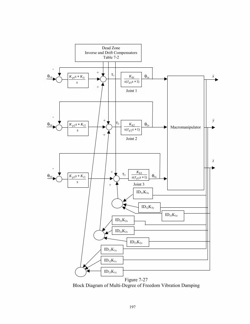
197

Figure 7-27 Block Diagram of Multi-Degree of Freedom Vibration Damping

+

+

+

Dead Zone Inverse and Drift Compensators

Table 7-2

Joint 1

+ -

τ1 θ1d θ1a Macromanipulator

Joint 2

+ -

τ2θ2d θ2a

Joint 3

+ -

τ3 θ3d θ3a

ID11K1x

ID12K1y

ID13K1z

ID21K2x

ID22K2y

ID23K2z

ID31K3x

ID32K3y

ID33K3z

1 1p iK s Ks+

2 2p iK s Ks+

3 3p iK s Ks+

1

1( 1)h

d

Ks sτ +

2

2( 1)h

d

Ks sτ +

3

3( 1)h

d

Ks sτ +

x&&

y&&

z&&

198

7.4.1 Disturbance Rejection

First, the vibration controller was tested in a configuration of (0°, 45°,-45°) and an

excitation was applied to the macromanipulator. The first case considered was with the

vibration controller turned on during the free vibration, and the resulting base vibration

and joint motion recorded. The second case was with the vibration controller on and a

disturbance is applied to the macromanipulator. A summary of the test cases and

calculated damping ratios is shown in Table 7-8. In most cases, two tests were performed

for each case and the damping ratios were averaged. In nearly all cases, as expected,

multiple modes were excited, but the lower frequency modes were those responsible for

the largest amplitude of vibration. In all of the test cases vibration energy is removed

from the overall system. The damping controller performance works best for damping

the fundamental mode at 1.2 Hz, which is the transverse mode of the first link in the y

direction. The controller gains for x direction vibration were selected to be low

compared to the y gains in order to help avoid excitation of the higher frequency modes,

notably modes at 4.2 and 9 Hz. A representative example of the recorded base position

and joint motion can be seen in Figures 7-28 and 7-29.

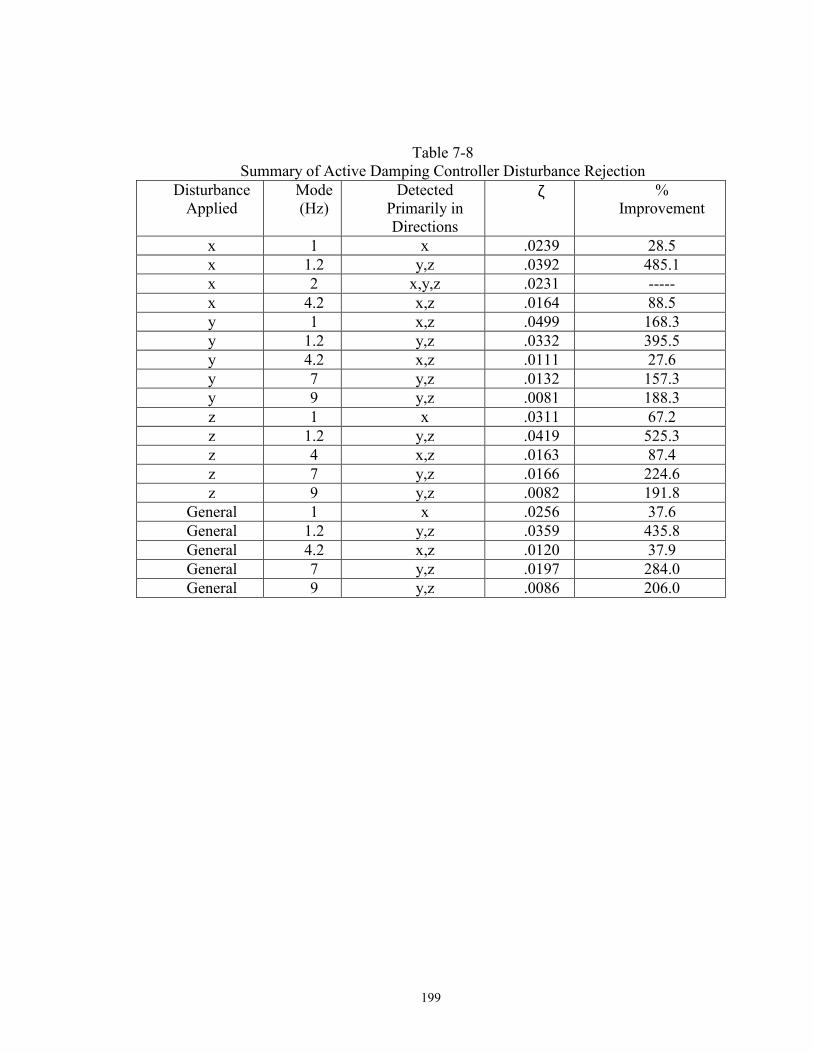
199

Table 7-8 Summary of Active Damping Controller Disturbance Rejection

Disturbance Applied

Mode (Hz)

Detected Primarily in Directions

ζ % Improvement

x 1 x .0239 28.5 x 1.2 y,z .0392 485.1 x 2 x,y,z .0231 ----- x 4.2 x,z .0164 88.5 y 1 x,z .0499 168.3 y 1.2 y,z .0332 395.5 y 4.2 x,z .0111 27.6 y 7 y,z .0132 157.3 y 9 y,z .0081 188.3 z 1 x .0311 67.2 z 1.2 y,z .0419 525.3 z 4 x,z .0163 87.4 z 7 y,z .0166 224.6 z 9 y,z .0082 191.8

General 1 x .0256 37.6 General 1.2 y,z .0359 435.8 General 4.2 x,z .0120 37.9 General 7 y,z .0197 284.0 General 9 y,z .0086 206.0

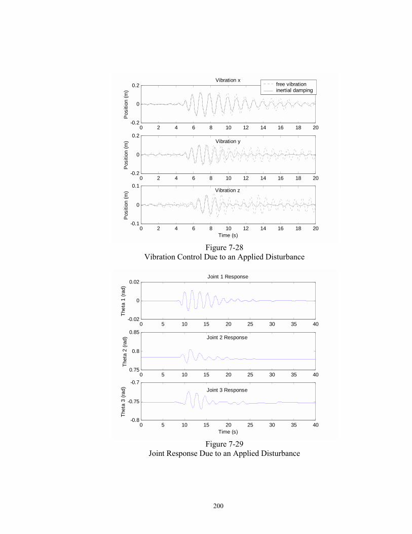
200

0 2 4 6 8 10 12 14 16 18 20-0.2

0

0.2Vibration x

Pos

ition

(m)

0 2 4 6 8 10 12 14 16 18 20-0.2

0

0.2Vibration y

Pos

ition

(m)

free vibration inertial damping

0 2 4 6 8 10 12 14 16 18 20-0.1

0

0.1Vibration z

Time (s)

Pos

ition

(m)

Figure 7-28

Vibration Control Due to an Applied Disturbance

0 5 10 15 20 25 30 35 40-0.02

0

0.02Joint 1 Response

Thet

a 1

(rad)

0 5 10 15 20 25 30 35 400.75

0.8

0.85Joint 2 Response

Thet

a 2

(rad)

0 5 10 15 20 25 30 35 40-0.8

-0.75

-0.7Joint 3 Response

Time (s)

Thet

a 3

(rad)

Figure 7-29

Joint Response Due to an Applied Disturbance

201

7.4.2 Combined Movement and Vibration Control

The second set of experiments was intended to verify the use of the performance

index to predict regions of good inertial damping performance. The robot was

commanded to move from a configuration of (-27°,0°,83°,0°,30°,90°) to

(45°,5°,60°,0°,90°,90°), which is one of the legs presented in section 6.3.4 for

simulated point-to-point motion in a configuration predicted better for inertial

damping performance. The resulting base vibration and commanded joint movement

may be seen in Figures 7-30 and 7-31. Note the very low amplitude of vibration in

the x and z directions compared with vibration in the y direction. The base vibration

with and without the vibration controller for the robot moving from (-27°,83°,-

100°,0°,90°,90°) to (45°,65°,-60°,0°,90°,90°), which is the alternate inverse

kinematics path, may be seen in Figure 7-32. As expected, lower amplitude of

vibration results in the regions of low coupling, but the vibration controller is much

less effective. The tradeoff in the better configuration is the impact on joint

positioning, since the controller requires small joint movements about the desired end

point position. These occurs primarily at the end of the path, although there are a few

correctional movements made just before the end of the trajectory which helps reduce

the level of vibration.

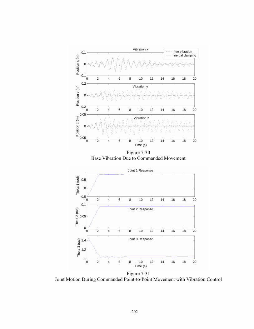
202

0 2 4 6 8 10 12 14 16 18 20-0.1

0

0.1Vibration x

Pos

ition

x (m

)

free vibration inertial damping

0 2 4 6 8 10 12 14 16 18 20-0.2

0

0.2Vibration y

Pos

ition

y (m

)

0 2 4 6 8 10 12 14 16 18 20-0.05

0

0.05Vibration z

Time (s)

Pos

ition

z (m

)

Figure 7-30

Base Vibration Due to Commanded Movement

0 2 4 6 8 10 12 14 16 18 20-0.5

0

0.5

Joint 1 Response

Thet

a 1

(rad)

0 2 4 6 8 10 12 14 16 18 200

0.05

0.1Joint 2 Response

Thet

a 2

(rad)

0 2 4 6 8 10 12 14 16 18 201

1.2

1.4 Joint 3 Response

Time (s)

Thet

a 3

(rad)

Figure 7-31

Joint Motion During Commanded Point-to-Point Movement with Vibration Control

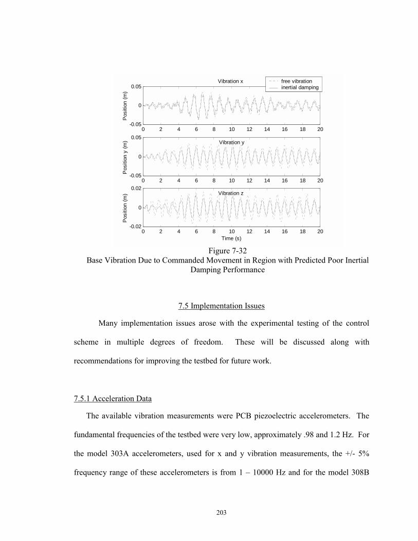
203

0 2 4 6 8 10 12 14 16 18 20-0.05

0

0.05Vibration x

Pos

ition

(m)

free vibration inertial damping

0 2 4 6 8 10 12 14 16 18 20-0.05

0

0.05Vibration y

Pos

ition

y (m

)

0 2 4 6 8 10 12 14 16 18 20-0.02

0

0.02Vibration z

Time (s)

Pos

ition

(m)

Figure 7-32

Base Vibration Due to Commanded Movement in Region with Predicted Poor Inertial Damping Performance

7.5 Implementation Issues

Many implementation issues arose with the experimental testing of the control

scheme in multiple degrees of freedom. These will be discussed along with

recommendations for improving the testbed for future work.

7.5.1 Acceleration Data

The available vibration measurements were PCB piezoelectric accelerometers. The

fundamental frequencies of the testbed were very low, approximately .98 and 1.2 Hz. For

the model 303A accelerometers, used for x and y vibration measurements, the +/- 5%

frequency range of these accelerometers is from 1 � 10000 Hz and for the model 308B

204

accelerometers is from 1 � 3000 Hz [57]. The modes of vibration on the new testbed

were very low and the accelerometers were operating toward the lower limit of their

useful range. This was further complicated by the beating phenomenon between the first

two fundamental modes discussed in Section 7.2.2. In addition, ideally, the measured

accelerations would need to be integrated as noted in section 5.4.5. As noted in several

sources [66,84], integration of piezoelectric acceleration time histories generally results

in calculated displacements that are dominated by large, low frequency drifts unless low

frequency spectral content is filtered out. In the case of the experimental hardware, it is

extremely important to get the fundamental (low) frequency modes of vibration and any

filtering would need to be performed real-time for use in the control scheme. The use of

a finite impulse response filter could be designed to avoid introduction of phasing, but

not implementable real-time. The use of an infinite impulse response or analog filter

could be used but higher order filters would be needed to provide a sharp enough cutoff

to avoid attenuation of the low frequency modes.

For lab implementation, a second order high pass digital Butterworth filter with a

cutoff frequency of .15 was used. This was necessary due to offsets in the accelerometer

data and it added little phase shift into the fundamental modes. For this work, it was

considered a reasonable approximation to use the measured acceleration data and it

provided reasonable performance. For future work, it is recommended that direct

position measurements be used that allow for very low frequency vibration measurement.

205

7.5.2 Hydraulics Effects

As discussed in Sections 6.4 and 7.2.1, it was assumed, and experimentally

verified by open loop testing, the hydraulic actuators followed a model of the form of

Equation 7-2. Figure 7-33 shows the commanded output from the PC (unitless) and the

resulting joint response at a low frequency command. The response is very nearly like an

integrator, as expected. The same comparison for a higher frequency commanded output

is shown in Figure 7-34, which shows much poorer tracking at higher frequencies. The

second order servovalve models and parameters in Table 7-1 do not predict this behavior.

Second order servovalve models were noted by the vendor as being a good

approximation at frequencies lower than 50 Hz [75,76]. However, the observed behavior

indicates that a higher order system model is required for accuracy. Merritt [50]

recommends a third or fourth order system model, depending on the accuracy of the

model required. For future work it is recommended that higher order servovalve models

be developed from system testing. Better high frequency response could then be obtained

by developing phase compensators from the known models.

206

4 4.5 5 5.5 6 6.5 7 7.5 8-200

-150

-100

-50

0

50

100

150

200Low Frequency Tracking of Joint 2

Time (s)

Tau

2 (u

nitle

ss)/T

heta

2 (r

ads)

Tau 2 Theta 2 (magnified)

Figure 7-33

Low Frequency Tracking of Joint 2

4.2 4.3 4.4 4.5 4.6 4.7 4.8-100

-80

-60

-40

-20

0

20

40

60

80

100High Frequency Tracking of Joint 2

Time (s)

Tau

(uni

tless

)/The

ta 2

(rad

)

Tau 2 Theta 2 (magnified)

Figure 7-34

High Frequency Tracking of Joint 2

207

7.5.3 Joint Torque Effects

The vibration controller gives reasonably good performance in approximately half

of the workspace. Whenever the robot is facing away from the macromanipulator, the

controller does not function properly to remove energy from the system (Figure 7-35).

This is due to a combination of two reasons. First, joint 1 provides a direct, amplified

input into the torsional mode of the first link in these configurations. As discussed in

Section 6.3.2, when the interaction torques are not considered it makes little difference in

the controller performance in some workspace configurations. However, in the

configuration shown in Figure 7-35, the interaction torques have a much greater effect on

the performance of the vibration controller and should be included in the controller. This

effect is magnified even more on the testbed due to the additonal leverage provided by

the second flexible link. Given the mode shape equation in 3-9, the torsional mode shape

is largest at the tip of the beam, hence application of the torque here has the greatest

effect in exciting it. This direct excitation combined with poor high frequency tracking,

as discussed in Sections 6.4 and 7.5.2, rendered these configurations unusable for active

damping on the current testbed.

As an example, consider the top view of the macro/micromanipulator shown at the

bottom of Figure 7-35. The figure on the left shows a configuration of poor inertial

damping performance, while the figure on the right shows a configuration in which the

controller performed better. Recall the generalized forces due to the micromanipulator

are given by equation 3-17. In the case on the left, the interaction forces remove

vibrational energy from the system, but the torques may add energy. In the case on the

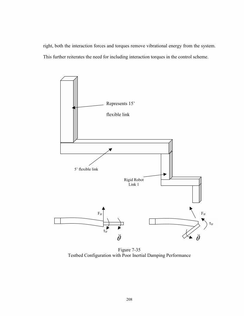
208

right, both the interaction forces and torques remove vibrational energy from the system.

This further reiterates the need for including interaction torques in the control scheme.

Figure 7-35

Testbed Configuration with Poor Inertial Damping Performance

τIF

τIF

Represents 15�

flexible link

5� flexible link

Rigid Robot Link 1

FIF FIF

θ&& θ&&

209

CHAPTER VIII

CONCLUSIONS

7.1 Conclusions This dissertation has developed, simulated, and demonstrated a position and

enhanced vibration control scheme for a macro/micromanipulator. The analogous case of

a rigid manipulator attached to a flexible but unactuated base was used to study the

directly controllable inertial interaction forces and torques acting between the robot and

its base. The �inertial singularities� in the joint workspace were investigated in detail,

namely the regions where the robot loses its ability to create interactions in one or more

degrees of freedom. A performance index was developed to predict the ability of the

robot to generate interactions and can be used to ensure the robot operates in joint space

configurations favorable for inertial damping. It was shown that when this is used along

with the appropriate choice of vibration control feedback gains, the inertia effects, or

those directly due to accelerating the links of the robot, have the greatest influence on the

interactions. By commanding the link accelerations proportional to the base vibration,

energy will be removed from the system. The vibration control signal is added to the

position control signal. Simulated and measured interaction forces and torques generated

at the base of a rigid robot were compared to verify conclusions drawn about the

210

controllable interactions. In addition, simulation and experimental results demonstrated

the combined position control and vibration damping ability of the scheme.

The true contributions began in Chapter 4 with a detailed discussion of the

controllable interaction force and torques. A performance measure was introduced which

predicts the effectiveness of the rigid robot in creating these interactions. The rigid

inertia effects (Bf, Bτ0) were studied in more detail and the �inertial singularities�

investigated. It was pointed out that these singularities are, in general, different from the

kinematic singularities. However, since the variation in performance is governed by the

joint space configuration of the rigid robot, the performance measure could be used to

quickly assess predicted inertial damping performance at the multiple inverse kinematic

joint space solutions and used to operate the rigid robot in configurations better suited for

inertial damping.

The inertia effects dominate the interactions in most non-singular configurations, but

in certain cases, the nonlinear rigid effects may also become significant and these cases

are discussed. The control scheme was discussed in Chapter 5. The vibration controller

requires an inverse dynamics function to cancel the most important coupled interaction

effects. Guidelines on choosing controller gains to ensure the inertia effects are the

dominant terms were presented.

Simulation results were presented in Chapter 6 demonstrating vibration damping of a

three degree of freedom anthropomorphic robot mounted on a flexible base. Simulations

demonstrating disturbance rejection as well as the use of the performance index in

predicting better joint space configurations for vibration damping during commanded

211

motion were included. Chapter 7 discussed the experimental testbed and presented

results from two areas of testing. The first was verification of the interaction force and

torque effects and work discussed in Chapter 4. The second was implementation of the

vibration control scheme on a multi-degree of freedom experimental testbed. Although

there were problems that arose with damping in certain workspace configurations, in

most of the workspace the vibration controller performed well to remove energy from the

system. This included both disturbance rejection as well as vibration control during

commanded movements. Finally, implementation issues were discussed.

7.2 Contributions Contributions of this work are:

1. Extension of the macro/micromanipulator control problem to multiple degrees of

freedom by considering the analogous problem of a rigid manipulator mounted on a

flexible base.

2. Detailed investigation of inertial singularities and variation in performance

throughout the workspace and development of a performance measure that predicts

the ability of the micromanipulator to effectively damp base vibration using an

inertial damping scheme.

3. Development of a control scheme that provides active base vibration damping in

parallel with rigid robot position control. This includes the use of the performance

index to improve the vibration damping capability of the micromanipulator given a

desired end point position and establishing appropriate limits on control gains.

212

4. Verification of the above control scheme via simulation

5. Verification of the above control scheme via experimental work. This included

verification of the accuracy of the interaction force and torque predictions and

demonstration of the effectiveness of the control scheme on a realistic multi-degree of

freedom testbed.

This work primarily builds on that performed previously by Lee [11,33], Cannon

[15,16], Loper [12,42], and Lew [34-40]. This extends their work to include some

concepts introduced in space robotics research by Papadopoulos, Evangelos, and

Dubowsky [56] and Torres and Dubowsky [77-79]. In particular, this is the first work to

develop the complete interaction forces and torque effects for a macro/micromanipulator

and investigate the variation in performance throughout the workspace. In addition, this

is the first work to introduce �inertial singularities,� determine when and why they occur,

and propose a solution to work around them. This is also the first work to consider

multiple modes of vibration and propose control gain limits to ensure overall energy

removal from the system. Finally, this is the first work demonstrating multiple-degrees

of freedom of vibration damping on an experimental testbed, involving multiple joints

actuating cooperatively for vibration damping. Although the scheme could not be shown

to be effective in all configurations, mainly due to implementation issues and simplifying

assumptions made to scale the inverse dynamics function to an implementable level, this

work demonstrates a clear contribution to the field.

213

7.3 Recommendations for Future Research

There are many areas of research that could be further investigated including

implementation issues that were discussed in section 7.5. As noted in Chapters 6 and 7 a

more reasonable method of modeling the interaction torque effects is needed. The

algorithm described in Section 4.4 allowed for a much easier derivation of the interaction

forces than the symbolic method described in Section 3.3, but a similar method was not

found for the interaction torques. Mainly, the length of the interaction torque equations,

detailed in Section A.1.2 for the three degree of freedom case, made simulating and

studying them in detail cumbersome and unimplementable in practice. More work needs

to be done in this area, either to discover a much more efficient method of deriving

expressions for the interaction torques or eliminating effects that are less important.

The use of input shaping in combination with an inertial damping control scheme is

an area worthy of future research. Input shaping techniques are effective at reducing the

amplitude of vibration induced by commanded movements but typically do not add

damping to the system. This becomes particularly noticeable in an example such as that

shown in section 6.3.4 and 7.4.2, where damping was compared for commanded rigid

robot movement with and without inertial damping. If implemented with input shaping,

vibration created by motion of the robot itself would be reduced and, assuming the robot

is operating in a region of predicted good performance, the controller could still provide

disturbance rejection. Hence, the combination of the two schemes should provide the

best performance for both commanded movement vibration control as well as disturbance

rejection.

214

Another area worthy of future research is the effect of implementation of the control

scheme on a digital controller. Simulations as well as experimental work were performed

using continuous system theory. Implementation involved real-time calculation of the

control signals during each control loop, based on sampling the appropriate control

signals (positions and accelerations). However, with increased computation time, which

will occur especially if interaction torques are included, sample and hold effects as well

as finite precision effects may become more of an issue.

Another area that should be considered is implementation of the proposed

controller with a macromanipulator at varying joint angles. This would change the

natural frequencies and damping ratios of the modes of vibration, as well as the

orientation of the applied interaction forces. The proposed controller should theoretically

apply as long as the frequency of vibration is measurable, but other unforeseen problems

could occur.

As discussed in section 6.3.1, vibration control performance is not as efficient in

regions of high nonlinear effects when higher modes exist in the system, which requires

lower control gains. Performance could possibly be improved by canceling those effects

in the vibration control scheme or using some alternate controller form. Another area of

future research should consider the effect of contact on the tip of the micromanipulator.

The work performed thus far assumes no contact on the system, whereas the more

general case would likely involve contact by the micromanipulator. Appropriate

modifications to the controller and/or inverse dynamics function may be necessary in

these cases.

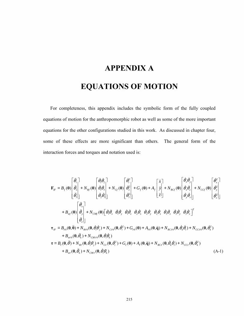
215

APPENDIX A

EQUATIONS OF MOTION

For completeness, this appendix includes the symbolic form of the fully coupled

equations of motion for the anthropomorphic robot as well as some of the more important

equations for the other configurations studied in this work. As discussed in chapter four,

some of these effects are more significant than others. The general form of the

interaction forces and torques and notation used is:

221 1 2 1

2 22 1 3 2

2 23 32 3

( ) ( ) ( ) ( ) ( ) ( )

x y x

IF f Rf Cf f f RCf x z CCf y

y z z

xB N N G A y N N

z

θ θ θθ θ θ θθ θ θ θ θ θ θθ θθ θ θ θ θ

= + + + + + +

F θ θ θ θ θ θ

& & &&& & & & &&&& & & & & & &&&

&& && & & &&& &

1 1 1 2 2 2 3 3 3

2 20 0 0 0 0 0 0

( ) ( )

( , ) ( , ) ( , ) ( ) ( , ) ( , ) ( , )

xT

wf y CMf x y z x y z x y z

z

IF R i j C i RC k l CC k

B N

B N N G A N Nτ τ τ τ τ τ τ

θθ θ θ θ θ θ θ θ θ θ θ θ θ θ θ θ θ θ θ

θ

θθ θ θ θ θ

+ +

= + + + + + +

θ θ

τ θ θ θ θ θ θ q θ θ

&&

&& & & & & & & & & & & & & & & & & & &

&&

&& & & & & & &&&

0 0

2 2

( , ) ( , )

( , ) ( , ) ( , ) ( ) ( , ) ( , ) ( , )

( , ) ( , )

w k CM i k

R i j C i RC k l CC k

w k CM i k

B N

B N N G A N N

B N

τ τ

τ τ τ τ τ τ τ

τ τ

θ θ θθ θθ θ θ θ θ

θ θθ

+ +

= + + + + + +

+ +

θ θτ θ θ θ θ θ q θ θ

θ θ

&& & &

&& & & & & &&&

&& & (A-1)

216

where:

B matrices are rigid body inertia-like matrices (Bτ is the inertia matrix) NR matrices are rigid body coriolis effects NC matrices are rigid body centrifugal effects G matrices are rigid body gravity effects A are flexible body inertia matrices (due to base acceleration) NRC are flexible body coriolis effects (due to base rotational velocities) NCC are flexible body centrifugal effects (due to base rotational velocities) BW are flexible body rotational inertia matrices (due to base rotational accelerations) NCM are cross coupling effects due to both joint velocities and base rotational velocities

This notation will be used for all robot configurations studied in this work. As

discussed in Chapter 3, equations were derived from a Matlab m-file using a Newton

Euler method. Due to their length and complexity, great pain was taken to find forms

that are more useful for the critical rigid and flexible inertia and nonlinear rigid effects.

However, due to the complexity of the equations this was only done for the some of the

equations. The remainder are included in the general (�simple� format) form provided by

Matlab.

A.1 Three Degree of Freedom Anthropomorphic Robot

The anthropomorphic robot configuration used here is similar to that used in

experimental work. The same link parameters and Denavit-Hartenberg parameters were

used as for the actual robot and the parameters are defined Figure 4-1. Notice the

alternate definition of joint angle two. This was chosen because software code was

already written to control the robot using these parameters and it avoided numerous

changes to the software code. The Denavit and Hartenberg parameters are shown in

Table A-1.

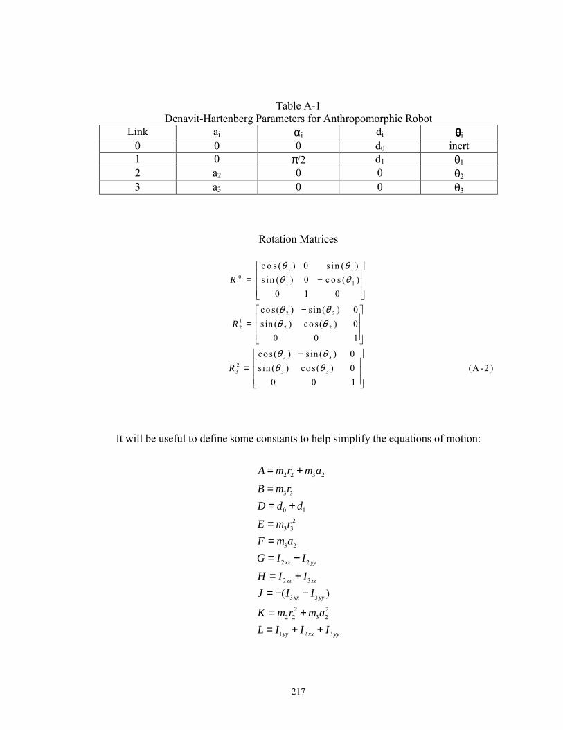
217

Table A-1 Denavit-Hartenberg Parameters for Anthropomorphic Robot

Link ai αi di θθθθi 0 0 0 d0 inert 1 0 π/2 d1 θ1 2 a2 0 0 θ2 3 a3 0 0 θ3

Rotation Matrices

1 10

1 1 1

c o s ( ) 0 s in ( )s in ( ) 0 c o s ( ) 0 1 0

Rθ θθ θ

= −

2 212 2 2

co s( ) s in ( ) 0s in ( ) co s( ) 0 0 0 1

Rθ θθ θ

− =

3 323 3 3

co s( ) s in ( ) 0s in ( ) co s( ) 0 (A -2 ) 0 0 1

Rθ θθ θ

− =

It will be useful to define some constants to help simplify the equations of motion:

2 2 3 2

3 3

0 1

23 3

3 2

2 2

2 3

3 3

2 22 2 3 2

1 2 3

( )

xx yy

zz zz

xx yy

yy xx yy

A m r m aB m rD d dE m rF m aG I IH I IJ I I

K m r m aL I I I

= +

== +

=== −

= += − −

= += + +

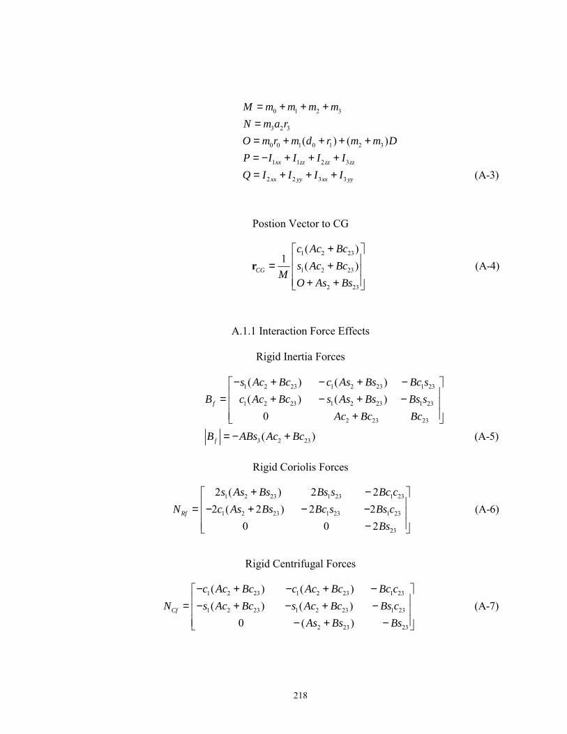
218

0 1 2 3

3 2 3

0 0 1 0 1 2 3

1 1 2 3

2 2 3 3

( ) ( )

(A-3)

xx zz zz zz

xx yy xx yy

M m m m mN m a rO m r m d r m m DP I I I IQ I I I I

= + + +== + + + += − + + += + + +

Postion Vector to CG

1 2 23

1 2 23

2 23

( )1 ( ) (A-4)CG

c Ac Bcs Ac Bc

MO As Bs

+ = + + +

r

A.1.1 Interaction Force Effects

Rigid Inertia Forces

1 2 23 1 2 23 1 23

1 2 23 1 2 23 1 23

2 23 23

3 2 23

( ) ( ) ( ) ( ) 0

( )

f

f

s Ac Bc c As Bs Bc sB c Ac Bc s As Bs Bs s

Ac Bc Bc

B ABs Ac Bc

− + − + − = + − + − +

= − + (A-5)

Rigid Coriolis Forces

1 2 23 1 23 1 23

1 2 23 1 23 1 23

23

2 ( ) 2 22 ( 2 ) 2 2 (A-6)

0 0 2 Rf

s As Bs Bs s Bc cN c As Bs Bc s Bs c

Bs

+ − = − + − − −

Rigid Centrifugal Forces

1 2 23 1 2 23 1 23

1 2 23 1 2 23 1 23

2 23 23

( ) ( ) ( ) ( ) (A-7)

0 ( ) Cf

c Ac Bc c Ac Bc Bc cN s Ac Bc s Ac Bc Bs c

As Bs Bs

− + − + − = − + − + − − + −

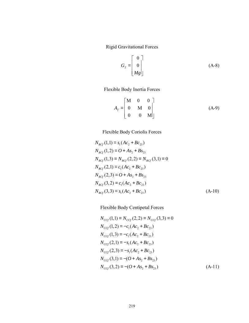
219

Rigid Gravitational Forces

0 0 (A-8)fG

Mg

=

Flexible Body Inertia Forces

M 0 0 0 M 0 (A-9) 0 0 M

fA =

Flexible Body Coriolis Forces

1 2 23

2 23

1 2 23

2 23

1 2 23

1 2 23

(1,1) ( )

(1,2)

(1,3) (2, 2) (3,1) 0

(2,1) ( )

(2,3)

(3, 2) ( )

(3,3) ( )

RCf

RCf

RCf RCf RCf

RCf

RCf

RCf

RCf

N s Ac BcN O As BsN N NN c Ac BcN O As BsN c Ac BcN s Ac Bc

= +

= + +

= = =

= +

= + +

= +

= + (A-10)

Flexible Body Centipetal Forces

1 2 23

1 2 23

1 2 23

1 2 23

2 23

2 23

(1,1) (2, 2) (3,3) 0

(1, 2) ( )

(1,3) ( )

(2,1) ( )

(2,3) ( )

(3,1) ( )

(3,2) ( )

CCf CCf CCf

CCf

CCf

CCf

CCf

CCf

CCf

N N NN c Ac BcN c Ac BcN s Ac BcN s Ac BcN O As BsN O As Bs

= = =

= − +

= − +

= − +

= − +

= − + +

= − + + (A-11)

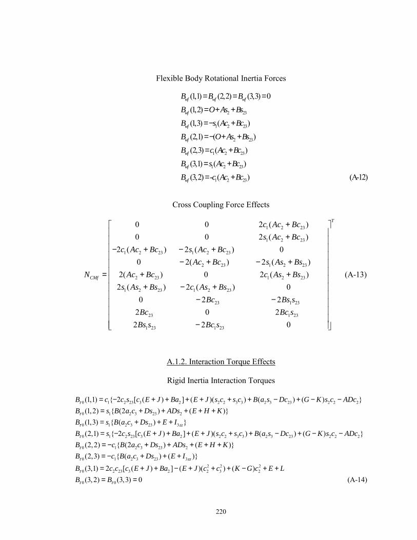
220

Flexible Body Rotational Inertia Forces

2 23

1 2 23

2 23

1 2 23

1 2 23

1 2 23

(1,1) (2,2) (3,3) 0

(1,2)

(1,3) ( )

(2,1) ( )

(2,3) ( )

(3,1) ( )

(3,2) - ( )

wf wf wf

wf

wf

wf

wf

wf

wf

B B BB O As BsB s Ac BcB O As BsB c Ac BcB s Ac BcB c Ac Bc

= = =

= + +

=− +

=− + +

= +

= +

= + (A-12)

Cross Coupling Force Effects

1 2 23

1 2 23

1 2 23 1 2 23

0 0 2 ( ) 0 0 2 ( )

2 ( ) 2 (

CMf

c Ac Bcs Ac Bc

c Ac Bc s Ac Bc

N

++

− + − +

=2 23 1 2 23

2 23 1 2 23

1 2 23 1 2

) 0 0 2( ) 2 ( ) 2( ) 0 2 ( ) 2 ( ) 2 (

Ac Bc s As BsAc Bc c As Bs

s As Bs c As

− + − ++ ++ − 23

23 1 23

23 1 23

) 0 0 2 2 2 0 2

BsBc Bs s

Bc Bc s

+− −

1 23 1 23

(A-13)

2 2 0

T

Bs s Bc s

−

A.1.2. Interaction Torque Effects

Rigid Inertia Interaction Torques

0 1 2 23 3 2 2 2 3 3 2 3 23 2 2 2

0 1 2 3 23 2

0 1 2 3 23 3

0 1 2 23 3 2 2 2 3 3

(1,1) { 2 [ ( ) ] ( )( ) ( ) ( ) }(1,2) { (2 ) ( )}(1,3) { ( ) }(2,1) { 2 [ ( ) ] ( )( )

zz

B c c s c E J Ba E J s c s c B a s Dc G K s c ADcB s B a c Ds ADs E H KB s B a c Ds E IB s c s c E J Ba E J s c s c B

τ

τ

τ

τ

= − + + + + + + − + − −= + + + + += + + += − + + + + + + 2 3 23 2 2 2

0 1 2 3 23 2

0 1 2 3 23 32 2 2

0 2 23 3 2 2 3 2

0 0

( ) ( ) }(2,2) { (2 ) ( )}(2,3) { ( ) ( )}

(3,1) 2 [ ( ) ] ( )( ) ( )(3,2) (3,3) 0

zz

a s Dc G K s c ADcB c B a c Ds ADs E H KB c B a c Ds E IB c c c E J Ba E J c c K G c E LB B

τ

τ

τ

τ τ

− + − −= − + + + + += − + + +

= + + − + + + − + += = (A-14)

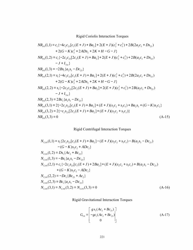
221

Rigid Coriolis Interaction Torques

2 20 1 2 23 3 2 2 3 2 3 23

22 2

2 20 1 2 23 3 2 2 3 2 3 23

3

(1,1) { 4 [ ( ) ] 2( )( ) 2 (2 )

2( ) 2 2 }

(1,2) { 2 [2 ( ) ] 2( )( ) 2 ( ) }zz

NR c c c c E J Ba E J c c B a c DsG K c ADs K H G J

NR c c c c E J Ba E J c c B a c DsJ I

NR

τ

τ

= − + + + + + + +

+ − + + + − −

= − + + + + + + +− +

0 1 2 3 23

2 20 1 2 23 3 2 2 3 2 3 23

22 2

2 20 1 2 23 3 2 2 3 2 3 23

(1,3) 2 { }

(2,1) { 4 [ ( ) ] 2( )( ) 2 (2 )

2( ) 2 2 }

(2,2) { 2 [2 ( ) ] 2( )( ) 2 ( )

Bs a s DcNR s c c c E J Ba E J c c B a c Ds

G K c ADs K H G JNR s c c c E J Ba E J c c B a c Ds

τ

τ

τ

= − −

= − + + + + + + +

+ − + + + − −

= − + + + + + + +

3

0 1 2 3 23

0 2 23 3 2 2 2 3 3 2 3 2 2

0 2 23 3 2 2 2 3 3

0

}(2,3) 2 { }(3,1) 2{ 2 [ ( ) ] ( )( ) ( ) }(3, 2) 2{ [2 ( ) ] ( )( )}(3,3) 0

zzJ INR Bc a s DcNR c s c E J Ba E J s c s c Ba s G K s cNR c s c E J Ba E J s c s cNR

τ

τ

τ

τ

− += −= − + + + + + + + −= − + + + + += (A-15)

Rigid Centrifugal Interaction Torques

0 1 2 23 3 2 2 2 3 3 2 3 23

2 2 2

0 1 2 23

0 1 2 3 23

0 1 2 23 3 2 2 2 3 3 2

(1,1) {2 [ ( ) ] ( )( ) ( ) ( ) }

(1,2) { }(1,3) { }(2,1) { 2 [ ( ) 2 ] ( )( ) (

C

C

C

C

N s c s c E J Ba E J s c s c B a s DcG K s c ADc

N Ds Ac BcN Bs a s DcN c c s c E J Ba E J s c s c B a s

τ

τ

τ

τ

= + + − + + − −− − += += − −= − + + + + + + 3 23

2 2 2

0 1 23 2

0 1 2 3 23

0 0 0

) ( ) }

(2,2) { }(2,3) { }(3,1) (3,2) (3,3) 0 (A-16)

C

C

C C C

DcG K s c ADc

N Dc Bc AcN Bc a s DcN N N

τ

τ

τ τ τ

−+ − −= − += −= = =

Rigid Gravitational Interaction Torques

1 2 23

0 1 2 23

s ( )( ) (A-17)

0

g Ac BcG gc Ac Bcτ

+ = − +

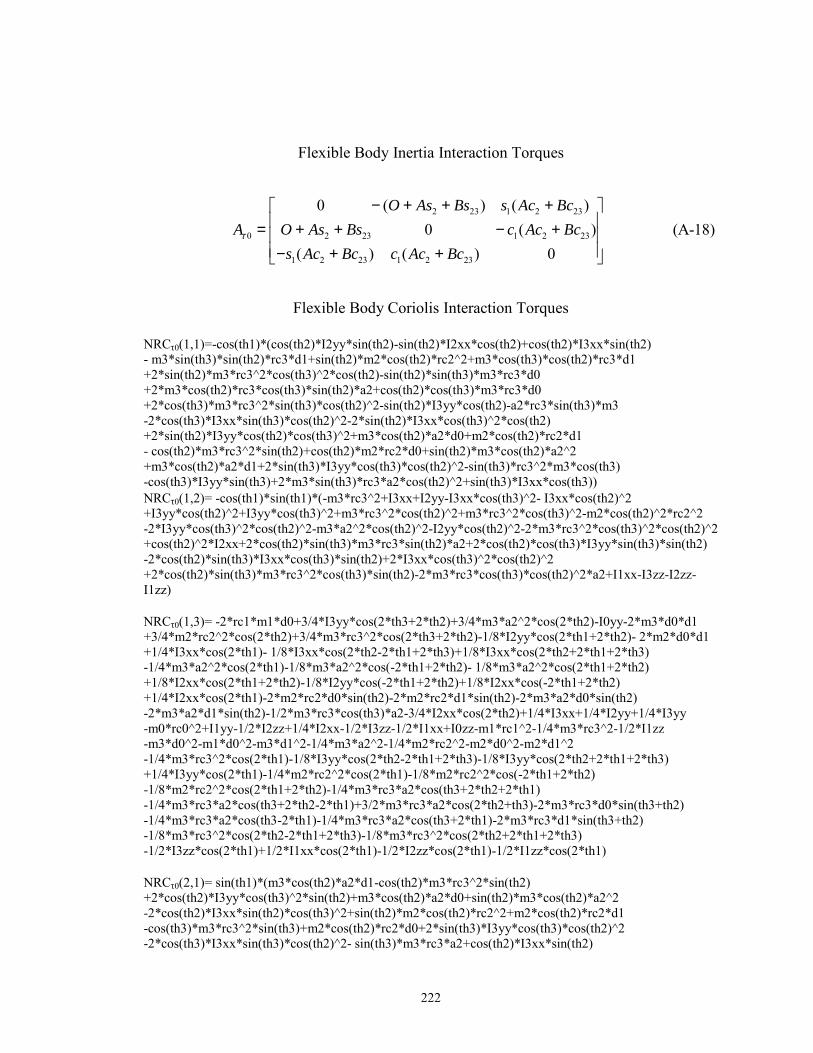
222

Flexible Body Inertia Interaction Torques

2 23 1 2 23

0 2 23 1 2 23

1 2 23 1 2 23

0 ( ) ( ) 0 ( ) (A-18)

( ) ( ) 0

O As Bs s Ac BcA O As Bs c Ac Bc

s Ac Bc c Ac Bcτ

− + + + = + + − + − + +

Flexible Body Coriolis Interaction Torques

NRCτ0(1,1)=-cos(th1)*(cos(th2)*I2yy*sin(th2)-sin(th2)*I2xx*cos(th2)+cos(th2)*I3xx*sin(th2) - m3*sin(th3)*sin(th2)*rc3*d1+sin(th2)*m2*cos(th2)*rc2^2+m3*cos(th3)*cos(th2)*rc3*d1 +2*sin(th2)*m3*rc3^2*cos(th3)^2*cos(th2)-sin(th2)*sin(th3)*m3*rc3*d0 +2*m3*cos(th2)*rc3*cos(th3)*sin(th2)*a2+cos(th2)*cos(th3)*m3*rc3*d0 +2*cos(th3)*m3*rc3^2*sin(th3)*cos(th2)^2-sin(th2)*I3yy*cos(th2)-a2*rc3*sin(th3)*m3 -2*cos(th3)*I3xx*sin(th3)*cos(th2)^2-2*sin(th2)*I3xx*cos(th3)^2*cos(th2) +2*sin(th2)*I3yy*cos(th2)*cos(th3)^2+m3*cos(th2)*a2*d0+m2*cos(th2)*rc2*d1 - cos(th2)*m3*rc3^2*sin(th2)+cos(th2)*m2*rc2*d0+sin(th2)*m3*cos(th2)*a2^2 +m3*cos(th2)*a2*d1+2*sin(th3)*I3yy*cos(th3)*cos(th2)^2-sin(th3)*rc3^2*m3*cos(th3) -cos(th3)*I3yy*sin(th3)+2*m3*sin(th3)*rc3*a2*cos(th2)^2+sin(th3)*I3xx*cos(th3)) NRCτ0(1,2)= -cos(th1)*sin(th1)*(-m3*rc3^2+I3xx+I2yy-I3xx*cos(th3)^2- I3xx*cos(th2)^2 +I3yy*cos(th2)^2+I3yy*cos(th3)^2+m3*rc3^2*cos(th2)^2+m3*rc3^2*cos(th3)^2-m2*cos(th2)^2*rc2^2 -2*I3yy*cos(th3)^2*cos(th2)^2-m3*a2^2*cos(th2)^2-I2yy*cos(th2)^2-2*m3*rc3^2*cos(th3)^2*cos(th2)^2 +cos(th2)^2*I2xx+2*cos(th2)*sin(th3)*m3*rc3*sin(th2)*a2+2*cos(th2)*cos(th3)*I3yy*sin(th3)*sin(th2) -2*cos(th2)*sin(th3)*I3xx*cos(th3)*sin(th2)+2*I3xx*cos(th3)^2*cos(th2)^2 +2*cos(th2)*sin(th3)*m3*rc3^2*cos(th3)*sin(th2)-2*m3*rc3*cos(th3)*cos(th2)^2*a2+I1xx-I3zz-I2zz-I1zz) NRCτ0(1,3)= -2*rc1*m1*d0+3/4*I3yy*cos(2*th3+2*th2)+3/4*m3*a2^2*cos(2*th2)-I0yy-2*m3*d0*d1 +3/4*m2*rc2^2*cos(2*th2)+3/4*m3*rc3^2*cos(2*th3+2*th2)-1/8*I2yy*cos(2*th1+2*th2)- 2*m2*d0*d1 +1/4*I3xx*cos(2*th1)- 1/8*I3xx*cos(2*th2-2*th1+2*th3)+1/8*I3xx*cos(2*th2+2*th1+2*th3) -1/4*m3*a2^2*cos(2*th1)-1/8*m3*a2^2*cos(-2*th1+2*th2)- 1/8*m3*a2^2*cos(2*th1+2*th2) +1/8*I2xx*cos(2*th1+2*th2)-1/8*I2yy*cos(-2*th1+2*th2)+1/8*I2xx*cos(-2*th1+2*th2) +1/4*I2xx*cos(2*th1)-2*m2*rc2*d0*sin(th2)-2*m2*rc2*d1*sin(th2)-2*m3*a2*d0*sin(th2) -2*m3*a2*d1*sin(th2)-1/2*m3*rc3*cos(th3)*a2-3/4*I2xx*cos(2*th2)+1/4*I3xx+1/4*I2yy+1/4*I3yy -m0*rc0^2+I1yy-1/2*I2zz+1/4*I2xx-1/2*I3zz-1/2*I1xx+I0zz-m1*rc1^2-1/4*m3*rc3^2-1/2*I1zz -m3*d0^2-m1*d0^2-m3*d1^2-1/4*m3*a2^2-1/4*m2*rc2^2-m2*d0^2-m2*d1^2 -1/4*m3*rc3^2*cos(2*th1)-1/8*I3yy*cos(2*th2-2*th1+2*th3)-1/8*I3yy*cos(2*th2+2*th1+2*th3) +1/4*I3yy*cos(2*th1)-1/4*m2*rc2^2*cos(2*th1)-1/8*m2*rc2^2*cos(-2*th1+2*th2) -1/8*m2*rc2^2*cos(2*th1+2*th2)-1/4*m3*rc3*a2*cos(th3+2*th2+2*th1) -1/4*m3*rc3*a2*cos(th3+2*th2-2*th1)+3/2*m3*rc3*a2*cos(2*th2+th3)-2*m3*rc3*d0*sin(th3+th2) -1/4*m3*rc3*a2*cos(th3-2*th1)-1/4*m3*rc3*a2*cos(th3+2*th1)-2*m3*rc3*d1*sin(th3+th2) -1/8*m3*rc3^2*cos(2*th2-2*th1+2*th3)-1/8*m3*rc3^2*cos(2*th2+2*th1+2*th3) -1/2*I3zz*cos(2*th1)+1/2*I1xx*cos(2*th1)-1/2*I2zz*cos(2*th1)-1/2*I1zz*cos(2*th1) NRCτ0(2,1)= sin(th1)*(m3*cos(th2)*a2*d1-cos(th2)*m3*rc3^2*sin(th2) +2*cos(th2)*I3yy*cos(th3)^2*sin(th2)+m3*cos(th2)*a2*d0+sin(th2)*m3*cos(th2)*a2^2 -2*cos(th2)*I3xx*sin(th2)*cos(th3)^2+sin(th2)*m2*cos(th2)*rc2^2+m2*cos(th2)*rc2*d1 -cos(th3)*m3*rc3^2*sin(th3)+m2*cos(th2)*rc2*d0+2*sin(th3)*I3yy*cos(th3)*cos(th2)^2 -2*cos(th3)*I3xx*sin(th3)*cos(th2)^2- sin(th3)*m3*rc3*a2+cos(th2)*I3xx*sin(th2)

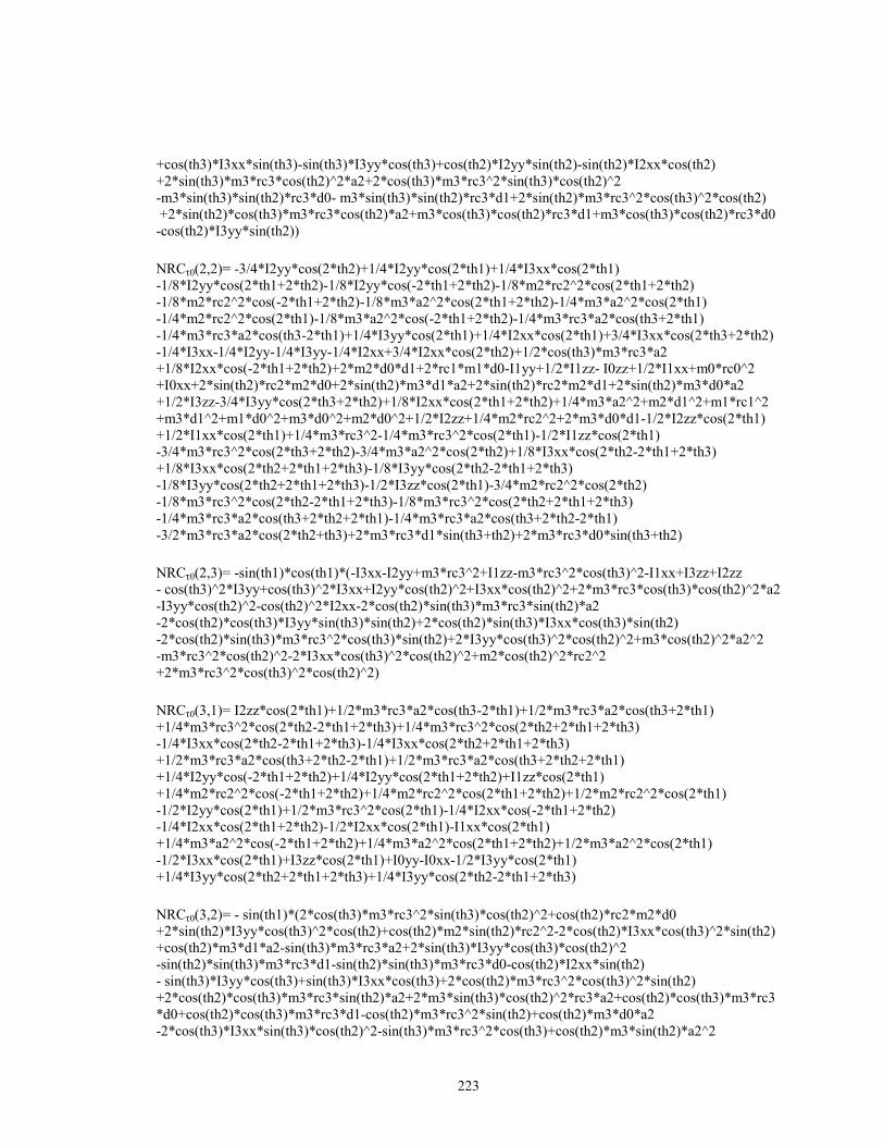
223

+cos(th3)*I3xx*sin(th3)-sin(th3)*I3yy*cos(th3)+cos(th2)*I2yy*sin(th2)-sin(th2)*I2xx*cos(th2) +2*sin(th3)*m3*rc3*cos(th2)^2*a2+2*cos(th3)*m3*rc3^2*sin(th3)*cos(th2)^2 -m3*sin(th3)*sin(th2)*rc3*d0- m3*sin(th3)*sin(th2)*rc3*d1+2*sin(th2)*m3*rc3^2*cos(th3)^2*cos(th2) +2*sin(th2)*cos(th3)*m3*rc3*cos(th2)*a2+m3*cos(th3)*cos(th2)*rc3*d1+m3*cos(th3)*cos(th2)*rc3*d0 -cos(th2)*I3yy*sin(th2)) NRCτ0(2,2)= -3/4*I2yy*cos(2*th2)+1/4*I2yy*cos(2*th1)+1/4*I3xx*cos(2*th1) -1/8*I2yy*cos(2*th1+2*th2)-1/8*I2yy*cos(-2*th1+2*th2)-1/8*m2*rc2^2*cos(2*th1+2*th2) -1/8*m2*rc2^2*cos(-2*th1+2*th2)-1/8*m3*a2^2*cos(2*th1+2*th2)-1/4*m3*a2^2*cos(2*th1) -1/4*m2*rc2^2*cos(2*th1)-1/8*m3*a2^2*cos(-2*th1+2*th2)-1/4*m3*rc3*a2*cos(th3+2*th1) -1/4*m3*rc3*a2*cos(th3-2*th1)+1/4*I3yy*cos(2*th1)+1/4*I2xx*cos(2*th1)+3/4*I3xx*cos(2*th3+2*th2) -1/4*I3xx-1/4*I2yy-1/4*I3yy-1/4*I2xx+3/4*I2xx*cos(2*th2)+1/2*cos(th3)*m3*rc3*a2 +1/8*I2xx*cos(-2*th1+2*th2)+2*m2*d0*d1+2*rc1*m1*d0-I1yy+1/2*I1zz- I0zz+1/2*I1xx+m0*rc0^2 +I0xx+2*sin(th2)*rc2*m2*d0+2*sin(th2)*m3*d1*a2+2*sin(th2)*rc2*m2*d1+2*sin(th2)*m3*d0*a2 +1/2*I3zz-3/4*I3yy*cos(2*th3+2*th2)+1/8*I2xx*cos(2*th1+2*th2)+1/4*m3*a2^2+m2*d1^2+m1*rc1^2 +m3*d1^2+m1*d0^2+m3*d0^2+m2*d0^2+1/2*I2zz+1/4*m2*rc2^2+2*m3*d0*d1-1/2*I2zz*cos(2*th1) +1/2*I1xx*cos(2*th1)+1/4*m3*rc3^2-1/4*m3*rc3^2*cos(2*th1)-1/2*I1zz*cos(2*th1) -3/4*m3*rc3^2*cos(2*th3+2*th2)-3/4*m3*a2^2*cos(2*th2)+1/8*I3xx*cos(2*th2-2*th1+2*th3) +1/8*I3xx*cos(2*th2+2*th1+2*th3)-1/8*I3yy*cos(2*th2-2*th1+2*th3) -1/8*I3yy*cos(2*th2+2*th1+2*th3)-1/2*I3zz*cos(2*th1)-3/4*m2*rc2^2*cos(2*th2) -1/8*m3*rc3^2*cos(2*th2-2*th1+2*th3)-1/8*m3*rc3^2*cos(2*th2+2*th1+2*th3) -1/4*m3*rc3*a2*cos(th3+2*th2+2*th1)-1/4*m3*rc3*a2*cos(th3+2*th2-2*th1) -3/2*m3*rc3*a2*cos(2*th2+th3)+2*m3*rc3*d1*sin(th3+th2)+2*m3*rc3*d0*sin(th3+th2) NRCτ0(2,3)= -sin(th1)*cos(th1)*(-I3xx-I2yy+m3*rc3^2+I1zz-m3*rc3^2*cos(th3)^2-I1xx+I3zz+I2zz - cos(th3)^2*I3yy+cos(th3)^2*I3xx+I2yy*cos(th2)^2+I3xx*cos(th2)^2+2*m3*rc3*cos(th3)*cos(th2)^2*a2 -I3yy*cos(th2)^2-cos(th2)^2*I2xx-2*cos(th2)*sin(th3)*m3*rc3*sin(th2)*a2 -2*cos(th2)*cos(th3)*I3yy*sin(th3)*sin(th2)+2*cos(th2)*sin(th3)*I3xx*cos(th3)*sin(th2) -2*cos(th2)*sin(th3)*m3*rc3^2*cos(th3)*sin(th2)+2*I3yy*cos(th3)^2*cos(th2)^2+m3*cos(th2)^2*a2^2 -m3*rc3^2*cos(th2)^2-2*I3xx*cos(th3)^2*cos(th2)^2+m2*cos(th2)^2*rc2^2 +2*m3*rc3^2*cos(th3)^2*cos(th2)^2) NRCτ0(3,1)= I2zz*cos(2*th1)+1/2*m3*rc3*a2*cos(th3-2*th1)+1/2*m3*rc3*a2*cos(th3+2*th1) +1/4*m3*rc3^2*cos(2*th2-2*th1+2*th3)+1/4*m3*rc3^2*cos(2*th2+2*th1+2*th3) -1/4*I3xx*cos(2*th2-2*th1+2*th3)-1/4*I3xx*cos(2*th2+2*th1+2*th3) +1/2*m3*rc3*a2*cos(th3+2*th2-2*th1)+1/2*m3*rc3*a2*cos(th3+2*th2+2*th1) +1/4*I2yy*cos(-2*th1+2*th2)+1/4*I2yy*cos(2*th1+2*th2)+I1zz*cos(2*th1) +1/4*m2*rc2^2*cos(-2*th1+2*th2)+1/4*m2*rc2^2*cos(2*th1+2*th2)+1/2*m2*rc2^2*cos(2*th1) -1/2*I2yy*cos(2*th1)+1/2*m3*rc3^2*cos(2*th1)-1/4*I2xx*cos(-2*th1+2*th2) -1/4*I2xx*cos(2*th1+2*th2)-1/2*I2xx*cos(2*th1)-I1xx*cos(2*th1) +1/4*m3*a2^2*cos(-2*th1+2*th2)+1/4*m3*a2^2*cos(2*th1+2*th2)+1/2*m3*a2^2*cos(2*th1) -1/2*I3xx*cos(2*th1)+I3zz*cos(2*th1)+I0yy-I0xx-1/2*I3yy*cos(2*th1) +1/4*I3yy*cos(2*th2+2*th1+2*th3)+1/4*I3yy*cos(2*th2-2*th1+2*th3) NRCτ0(3,2)= - sin(th1)*(2*cos(th3)*m3*rc3^2*sin(th3)*cos(th2)^2+cos(th2)*rc2*m2*d0 +2*sin(th2)*I3yy*cos(th3)^2*cos(th2)+cos(th2)*m2*sin(th2)*rc2^2-2*cos(th2)*I3xx*cos(th3)^2*sin(th2) +cos(th2)*m3*d1*a2-sin(th3)*m3*rc3*a2+2*sin(th3)*I3yy*cos(th3)*cos(th2)^2 -sin(th2)*sin(th3)*m3*rc3*d1-sin(th2)*sin(th3)*m3*rc3*d0-cos(th2)*I2xx*sin(th2) - sin(th3)*I3yy*cos(th3)+sin(th3)*I3xx*cos(th3)+2*cos(th2)*m3*rc3^2*cos(th3)^2*sin(th2) +2*cos(th2)*cos(th3)*m3*rc3*sin(th2)*a2+2*m3*sin(th3)*cos(th2)^2*rc3*a2+cos(th2)*cos(th3)*m3*rc3*d0+cos(th2)*cos(th3)*m3*rc3*d1-cos(th2)*m3*rc3^2*sin(th2)+cos(th2)*m3*d0*a2 -2*cos(th3)*I3xx*sin(th3)*cos(th2)^2-sin(th3)*m3*rc3^2*cos(th3)+cos(th2)*m3*sin(th2)*a2^2

224

-sin(th2)*I3yy*cos(th2)+cos(th2)*I3xx*sin(th2)+sin(th2)*I2yy*cos(th2)+cos(th2)*rc2*m2*d1) NRCτ0(3,3)= -cos(th1)*(sin(th2)*m3*rc3^2*cos(th2)-cos(th2)*rc2*m2*d0 -2*sin(th3)*I3yy*cos(th3)*cos(th2)^2+sin(th2)*sin(th3)*m3*rc3*d1-cos(th2)*m3*d0*a2 -2*sin(th2)*I3yy*cos(th3)^2*cos(th2)-cos(th2)*m3*sin(th2)*a2^2- cos(th2)*m3*d1*a2 +2*cos(th2)*I3xx*cos(th3)^2*sin(th2)+cos(th2)*I3yy*sin(th2)+sin(th3)*I3yy*cos(th3) -sin(th2)*I2yy*cos(th2)+cos(th2)*I2xx*sin(th2)-cos(th2)*I3xx*sin(th2) -2*cos(th2)*cos(th3)*m3*rc3*sin(th2)*a2-cos(th2)*cos(th3)*m3*rc3*d0 -2*cos(th2)*m3*rc3^2*cos(th3)^2*sin(th2)-cos(th2)*cos(th3)*m3*rc3*d1 -cos(th3)*I3xx*sin(th3)+m3*sin(th3)*rc3*a2-cos(th2)*m2*sin(th2)*rc2^2-cos(th2)*rc2*m2*d1 -2*cos(th3)*m3*rc3^2*sin(th3)*cos(th2)^2+sin(th2)*sin(th3)*m3*rc3*d0 -2*m3*sin(th3)*cos(th2)^2*rc3*a2+2*cos(th3)*I3xx*sin(th3)*cos(th2)^2+sin(th3)*m3*rc3^2*cos(th3))

(A-19)

Flexible Body Centrifugal Interaction Torques

NCCτ0(1,1)=0 NCCτ0(1,2)= sin(th1)*(-I3xx*sin(th2)*cos(th2)-cos(th2)*I2yy*sin(th2)- I3xx*sin(th3)*cos(th3) +I3yy*sin(th3)*cos(th3)+sin(th2)*I2xx*cos(th2)+I3yy*sin(th2)*cos(th2) -2*m3*rc3^2*cos(th3)^2*cos(th2)*sin(th2)-m3*rc3*cos(th3)*cos(th2)*d0-m3*rc3*cos(th3)*cos(th2)*d1 -2*m3*rc3*cos(th3)*cos(th2)*sin(th2)*a2+m3*rc3*sin(th3)*sin(th2)*d0 -2*m3*rc3*sin(th3)*a2*cos(th2)^2-2*m3*rc3^2*sin(th3)*cos(th3)*cos(th2)^2 +m3*rc3*sin(th3)*sin(th2)*d1-m3*cos(th2)*sin(th2)*a2^2- m3*cos(th2)*d1*a2 +2*I3xx*cos(th3)^2*cos(th2)*sin(th2)-rc2*m2*cos(th2)*d1-2*I3yy*cos(th3)^2*cos(th2)*sin(th2) -m3*cos(th2)*d0*a2+m3*rc3^2*sin(th2)*cos(th2)- m2*cos(th2)*sin(th2)*rc2^2 +2*I3xx*cos(th3)*cos(th2)^2*sin(th3)-2*I3yy*sin(th3)*cos(th3)*cos(th2)^2 -rc2*m2*cos(th2)*d0+m3*rc3^2*sin(th3)*cos(th3)+m3*rc3*sin(th3)*a2) NCCτ0(1,3)= sin(th1)*(cos(th2)*I2yy*sin(th2)-I3yy*sin(th3)*cos(th3)- I3yy*sin(th2)*cos(th2) +I3xx*sin(th2)*cos(th2)+2*m3*rc3*cos(th3)*cos(th2)*sin(th2)*a2+2*m3*rc3*sin(th3)*a2*cos(th2)^2 +m3*rc3*cos(th3)*cos(th2)*d0+2*m3*rc3^2*cos(th3)^2*cos(th2)*sin(th2)+m3*rc3*cos(th3)*cos(th2)*d1+2*m3*rc3^2*sin(th3)*cos(th3)*cos(th2)^2-2*I3xx*cos(th3)*cos(th2)^2*sin(th3) - m3*rc3*sin(th3)*sin(th2)*d0-m3*rc3*sin(th3)*sin(th2)*d1- sin(th2)*I2xx*cos(th2) +I3xx*sin(th3)*cos(th3)-m3*rc3*sin(th3)*a2-m3*rc3^2*sin(th3)*cos(th3)- m3*rc3^2*sin(th2)*cos(th2) +m3*cos(th2)*sin(th2)*a2^2+m3*cos(th2)*d0*a2+m2*cos(th2)*sin(th2)*rc2^2 -2*I3xx*cos(th3)^2*cos(th2)*sin(th2) +2*I3yy*sin(th3)*cos(th3)*cos(th2)^2 +m3*cos(th2)*d1*a2+rc2*m2*cos(th2)*d0+rc2*m2*cos(th2)*d1+2*I3yy*cos(th3)^2*cos(th2)*sin(th2)) NCCτ0(2,1)= cos(th1)*(-sin(th3)*I3yy*cos(th3)+cos(th3)*I3xx*sin(th3)-sin(th2)*I3yy*cos(th2) - sin(th2)*I2xx*cos(th2)+cos(th2)*I2yy*sin(th2)+cos(th2)*I3xx*sin(th2) +2*sin(th3)*m3*rc3^2*cos(th3)*cos(th2)^2- m3*rc3*sin(th3)*sin(th2)*d0 +2*m3*sin(th3)*rc3*a2*cos(th2)^2+2*sin(th2)*m3*rc3^2*cos(th3)^2*cos(th2) -m3*sin(th3)*sin(th2)*rc3*d1+2*cos(th3)*I3yy*sin(th3)*cos(th2)^2-2*sin(th2)*I3xx*cos(th3)^2*cos(th2) +sin(th2)*m2*cos(th2)*rc2^2+m3*rc3*cos(th3)*cos(th2)*d0+m3*cos(th3)*cos(th2)*rc3*d1 +m2*cos(th2)*rc2*d1+2*sin(th2)*cos(th3)*m3*rc3*cos(th2)*a2+m3*cos(th2)*d0*a2 +2*cos(th2)*I3yy*cos(th3)^2*sin(th2)-cos(th2)*m3*rc3^2*sin(th2)-2*cos(th3)*I3xx*sin(th3)*cos(th2)^2 -cos(th3)*m3*rc3^2*sin(th3)- m3*sin(th3)*rc3*a2+sin(th2)*m3*cos(th2)*a2^2 +m3*cos(th2)*a2*d1+rc2*m2*cos(th2)*d0) NCCτ0(2,2)=0

225

NCCτ0(2,3)= -cos(th1)*(-sin(th2)*I3yy*cos(th2)+cos(th3)*I3xx*sin(th3)- sin(th2)*I2xx*cos(th2) +cos(th2)*I3xx*sin(th2)- sin(th3)*I3yy*cos(th3)+2*sin(th2)*m3*rc3^2*cos(th3)^2*cos(th2) +2*m3*sin(th3)*rc3*a2*cos(th2)^2- m3*sin(th3)*sin(th2)*rc3*d1+m3*rc3*cos(th3)*cos(th2)*d0 +2*sin(th3)*m3*rc3^2*cos(th3)*cos(th2)^2+m3*cos(th3)*cos(th2)*rc3*d1- m3*rc3*sin(th3)*sin(th2)*d0 +2*sin(th2)*cos(th3)*m3*rc3*cos(th2)*a2-cos(th3)*m3*rc3^2*sin(th3)- cos(th2)*m3*rc3^2*sin(th2) +rc2*m2*cos(th2)*d0+sin(th2)*m3*cos(th2)*a2^2+m3*cos(th2)*a2*d1+sin(th2)*m2*cos(th2)*rc2^2 -2*sin(th2)*I3xx*cos(th3)^2*cos(th2)+m2*cos(th2)*rc2*d1+m3*cos(th2)*d0*a2 +2*cos(th3)*I3yy*sin(th3)*cos(th2)^2-m3*sin(th3)*rc3*a2+2*cos(th2)*I3yy*cos(th3)^2*sin(th2) -2*cos(th3)*I3xx*sin(th3)*cos(th2)^2+cos(th2)*I2yy*sin(th2)) NCCτ0(3,1)= -sin(th1)*cos(th1)*(I3zz+I2zz+rc2^2*cos(th2)^2*m2+a2^2*cos(th2)^2*m3 -2*cos(th2)^2*cos(th3)^2*I3xx-cos(th3)^2*rc3^2*m3- cos(th2)^2*rc3^2*m3 +2*cos(th3)^2*cos(th2)^2*I3yy-I3xx-I2yy+rc3^2*m3-cos(th3)^2*I3yy- cos(th2)^2*I3yy +2*cos(th2)^2*cos(th3)^2*rc3^2*m3+cos(th2)^2*I3xx+2*cos(th2)*cos(th3)*I3xx*sin(th3)*sin(th2) -2*cos(th2)*cos(th3)*rc3^2*m3*sin(th3)*sin(th2)+2*a2*cos(th2)^2*rc3*m3*cos(th3) -2*a2*cos(th2)*rc3*m3*sin(th3)*sin(th2)-2*cos(th2)*sin(th3)*I3yy*cos(th3)*sin(th2) -cos(th2)^2*I2xx+cos(th2)^2*I2yy+cos(th3)^2*I3xx-I1xx+I1zz) NCCτ0(3,2)= sin(th1)*cos(th1)*(I3zz+I2zz-I3xx-I2yy+rc3^2*m3-I1xx+I1zz- cos(th2)^2*I2xx +cos(th2)^2*I2yy+cos(th2)^2*I3xx- cos(th2)^2*I3yy+cos(th3)^2*I3xx +2*a2*cos(th2)^2*rc3*m3*cos(th3)-2*cos(th2)^2*cos(th3)^2*I3xx+2*cos(th2)^2*cos(th3)^2*rc3^2*m3 - cos(th3)^2*rc3^2*m3+a2^2*cos(th2)^2*m3+2*cos(th3)^2*cos(th2)^2*I3yy+rc2^2*cos(th2)^2*m2 +2*cos(th2)*cos(th3)*I3xx*sin(th3)*sin(th2)-2*cos(th2)*sin(th3)*I3yy*cos(th3)*sin(th2) -2*cos(th2)*cos(th3)*rc3^2*m3*sin(th3)*sin(th2)-cos(th3)^2*I3yy -2*a2*cos(th2)*rc3*m3*sin(th3)*sin(th2)-cos(th2)^2*rc3^2*m3) NCCτ0(3,3)=0 (A-20)

Flexible Body Rotational Inertia Interaction Torques Bw0(1,1)= 2*rc2*m2*sin(th2)*d1+2*m3*rc3*cos(th3)*a2- m3*rc3^2*cos(th1)^2 +I3yy*cos(th3)^2*cos(th1)^2-I3xx*cos(th1)^2*cos(th2)^2-2*I3yy*cos(th2)^2*cos(th1)^2*cos(th3)^2 -I2zz*cos(th1)^2+m3*d0^2+I3xx*cos(th1)^2+2*I3xx*cos(th3)^2*cos(th2)^2*cos(th1)^2 -I1zz*cos(th1)^2+I1zz+2*rc2*m2*sin(th2)*d0+m3*rc3^2+I1xx*cos(th1)^2+2*m3*sin(th2)*d0*a2 - I2yy*cos(th1)^2*cos(th2)^2+I3yy*cos(th2)^2*cos(th1)^2+2*m3*sin(th2)*d1*a2 +2*cos(th2)*sin(th3)*m3*rc3*sin(th2)*cos(th1)^2*a2-2*cos(th2)*I3xx*cos(th3)*sin(th3)*sin(th2)*cos(th1)^2-2*m3*rc3*cos(th3)*a2*cos(th1)^2*cos(th2)^2 +2*cos(th2)*sin(th3)*m3*rc3^2*cos(th3)*sin(th2)*cos(th1)^2 +2*cos(th2)*sin(th3)*I3yy*cos(th3)*sin(th2)*cos(th1)^2+2*m3*rc3*cos(th3)*sin(th2)*d0 +2*m3*rc3*sin(th3)*cos(th2)*d0- I3xx*cos(th1)^2*cos(th3)^2+I2xx*cos(th2)^2*cos(th1)^2 +2*rc1*m1*d0+2*m3*d0*d1+2*m2*d0*d1-m3*cos(th1)^2*a2^2*cos(th2)^2+m3*a2^2 -2*m3*rc3^2*cos(th2)^2*cos(th1)^2*cos(th3)^2+2*m3*rc3*cos(th3)*sin(th2)*d1 +2*m3*rc3*sin(th3)*cos(th2)*d1+I2zz+I3zz+I2yy*cos(th1)^2+m3*d1^2+m1*d0^2 -I3zz*cos(th1)^2+m3*rc3^2*cos(th2)^2*cos(th1)^2+I0xx+m0*rc0^2+m2*rc2^2+m2*d0^2+m1*rc1^2 +m2*d1^2-m2*rc2^2*cos(th1)^2*cos(th2)^2+m3*rc3^2*cos(th3)^2*cos(th1)^2 Bw0(1,2)= -cos(th1)*sin(th1)*(m3*rc3^2-I3xx-I2yy-m3*rc3^2*cos(th2)^2+m3*a2^2*cos(th2)^2 -2*I3xx*cos(th3)^2*cos(th2)^2+2*I3yy*cos(th3)^2*cos(th2)^2 -2*cos(th2)*sin(th3)*m3*rc3^2*cos(th3)*sin(th2)+2*cos(th2)*I3xx*cos(th3)*sin(th3)*sin(th2)

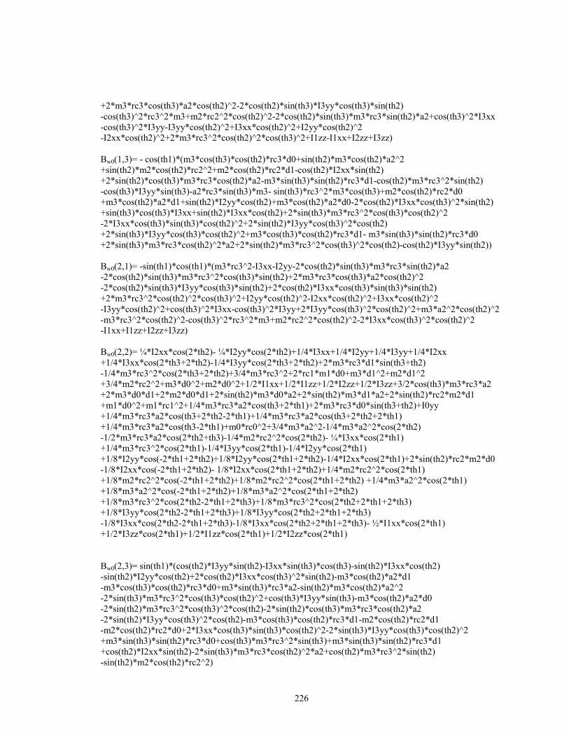
226

+2*m3*rc3*cos(th3)*a2*cos(th2)^2-2*cos(th2)*sin(th3)*I3yy*cos(th3)*sin(th2) -cos(th3)^2*rc3^2*m3+m2*rc2^2*cos(th2)^2-2*cos(th2)*sin(th3)*m3*rc3*sin(th2)*a2+cos(th3)^2*I3xx -cos(th3)^2*I3yy-I3yy*cos(th2)^2+I3xx*cos(th2)^2+I2yy*cos(th2)^2 -I2xx*cos(th2)^2+2*m3*rc3^2*cos(th2)^2*cos(th3)^2+I1zz-I1xx+I2zz+I3zz) Bw0(1,3)= - cos(th1)*(m3*cos(th3)*cos(th2)*rc3*d0+sin(th2)*m3*cos(th2)*a2^2 +sin(th2)*m2*cos(th2)*rc2^2+m2*cos(th2)*rc2*d1-cos(th2)*I2xx*sin(th2) +2*sin(th2)*cos(th3)*m3*rc3*cos(th2)*a2-m3*sin(th3)*sin(th2)*rc3*d1-cos(th2)*m3*rc3^2*sin(th2) -cos(th3)*I3yy*sin(th3)-a2*rc3*sin(th3)*m3- sin(th3)*rc3^2*m3*cos(th3)+m2*cos(th2)*rc2*d0 +m3*cos(th2)*a2*d1+sin(th2)*I2yy*cos(th2)+m3*cos(th2)*a2*d0-2*cos(th2)*I3xx*cos(th3)^2*sin(th2) +sin(th3)*cos(th3)*I3xx+sin(th2)*I3xx*cos(th2)+2*sin(th3)*m3*rc3^2*cos(th3)*cos(th2)^2 -2*I3xx*cos(th3)*sin(th3)*cos(th2)^2+2*sin(th2)*I3yy*cos(th3)^2*cos(th2) +2*sin(th3)*I3yy*cos(th3)*cos(th2)^2+m3*cos(th3)*cos(th2)*rc3*d1- m3*sin(th3)*sin(th2)*rc3*d0 +2*sin(th3)*m3*rc3*cos(th2)^2*a2+2*sin(th2)*m3*rc3^2*cos(th3)^2*cos(th2)-cos(th2)*I3yy*sin(th2)) Bw0(2,1)= -sin(th1)*cos(th1)*(m3*rc3^2-I3xx-I2yy-2*cos(th2)*sin(th3)*m3*rc3*sin(th2)*a2 -2*cos(th2)*sin(th3)*m3*rc3^2*cos(th3)*sin(th2)+2*m3*rc3*cos(th3)*a2*cos(th2)^2 -2*cos(th2)*sin(th3)*I3yy*cos(th3)*sin(th2)+2*cos(th2)*I3xx*cos(th3)*sin(th3)*sin(th2) +2*m3*rc3^2*cos(th2)^2*cos(th3)^2+I2yy*cos(th2)^2-I2xx*cos(th2)^2+I3xx*cos(th2)^2 -I3yy*cos(th2)^2+cos(th3)^2*I3xx-cos(th3)^2*I3yy+2*I3yy*cos(th3)^2*cos(th2)^2+m3*a2^2*cos(th2)^2 -m3*rc3^2*cos(th2)^2-cos(th3)^2*rc3^2*m3+m2*rc2^2*cos(th2)^2-2*I3xx*cos(th3)^2*cos(th2)^2 -I1xx+I1zz+I2zz+I3zz) Bw0(2,2)= ¼*I2xx*cos(2*th2)- ¼*I2yy*cos(2*th2)+1/4*I3xx+1/4*I2yy+1/4*I3yy+1/4*I2xx +1/4*I3xx*cos(2*th3+2*th2)-1/4*I3yy*cos(2*th3+2*th2)+2*m3*rc3*d1*sin(th3+th2) -1/4*m3*rc3^2*cos(2*th3+2*th2)+3/4*m3*rc3^2+2*rc1*m1*d0+m3*d1^2+m2*d1^2 +3/4*m2*rc2^2+m3*d0^2+m2*d0^2+1/2*I1xx+1/2*I1zz+1/2*I2zz+1/2*I3zz+3/2*cos(th3)*m3*rc3*a2 +2*m3*d0*d1+2*m2*d0*d1+2*sin(th2)*m3*d0*a2+2*sin(th2)*m3*d1*a2+2*sin(th2)*rc2*m2*d1 +m1*d0^2+m1*rc1^2+1/4*m3*rc3*a2*cos(th3+2*th1)+2*m3*rc3*d0*sin(th3+th2)+I0yy +1/4*m3*rc3*a2*cos(th3+2*th2-2*th1)+1/4*m3*rc3*a2*cos(th3+2*th2+2*th1) +1/4*m3*rc3*a2*cos(th3-2*th1)+m0*rc0^2+3/4*m3*a2^2-1/4*m3*a2^2*cos(2*th2) -1/2*m3*rc3*a2*cos(2*th2+th3)-1/4*m2*rc2^2*cos(2*th2)- ¼*I3xx*cos(2*th1) +1/4*m3*rc3^2*cos(2*th1)-1/4*I3yy*cos(2*th1)-1/4*I2yy*cos(2*th1) +1/8*I2yy*cos(-2*th1+2*th2)+1/8*I2yy*cos(2*th1+2*th2)-1/4*I2xx*cos(2*th1)+2*sin(th2)*rc2*m2*d0 -1/8*I2xx*cos(-2*th1+2*th2)- 1/8*I2xx*cos(2*th1+2*th2)+1/4*m2*rc2^2*cos(2*th1) +1/8*m2*rc2^2*cos(-2*th1+2*th2)+1/8*m2*rc2^2*cos(2*th1+2*th2) +1/4*m3*a2^2*cos(2*th1) +1/8*m3*a2^2*cos(-2*th1+2*th2)+1/8*m3*a2^2*cos(2*th1+2*th2) +1/8*m3*rc3^2*cos(2*th2-2*th1+2*th3)+1/8*m3*rc3^2*cos(2*th2+2*th1+2*th3) +1/8*I3yy*cos(2*th2-2*th1+2*th3)+1/8*I3yy*cos(2*th2+2*th1+2*th3) -1/8*I3xx*cos(2*th2-2*th1+2*th3)-1/8*I3xx*cos(2*th2+2*th1+2*th3)- ½*I1xx*cos(2*th1) +1/2*I3zz*cos(2*th1)+1/2*I1zz*cos(2*th1)+1/2*I2zz*cos(2*th1) Bw0(2,3)= sin(th1)*(cos(th2)*I3yy*sin(th2)-I3xx*sin(th3)*cos(th3)-sin(th2)*I3xx*cos(th2) -sin(th2)*I2yy*cos(th2)+2*cos(th2)*I3xx*cos(th3)^2*sin(th2)-m3*cos(th2)*a2*d1 -m3*cos(th3)*cos(th2)*rc3*d0+m3*sin(th3)*rc3*a2-sin(th2)*m3*cos(th2)*a2^2 -2*sin(th3)*m3*rc3^2*cos(th3)*cos(th2)^2+cos(th3)*I3yy*sin(th3)-m3*cos(th2)*a2*d0 -2*sin(th2)*m3*rc3^2*cos(th3)^2*cos(th2)-2*sin(th2)*cos(th3)*m3*rc3*cos(th2)*a2 -2*sin(th2)*I3yy*cos(th3)^2*cos(th2)-m3*cos(th3)*cos(th2)*rc3*d1-m2*cos(th2)*rc2*d1 -m2*cos(th2)*rc2*d0+2*I3xx*cos(th3)*sin(th3)*cos(th2)^2-2*sin(th3)*I3yy*cos(th3)*cos(th2)^2 +m3*sin(th3)*sin(th2)*rc3*d0+cos(th3)*m3*rc3^2*sin(th3)+m3*sin(th3)*sin(th2)*rc3*d1 +cos(th2)*I2xx*sin(th2)-2*sin(th3)*m3*rc3*cos(th2)^2*a2+cos(th2)*m3*rc3^2*sin(th2) -sin(th2)*m2*cos(th2)*rc2^2)

227

Bw0(3,1)= -cos(th1)*(cos(th2)*rc2*m2*d0+cos(th2)*m3*d0*a2-sin(th3)*m3*rc3^2*cos(th3) -sin(th3)*m3*rc3*a2+cos(th2)*cos(th3)*m3*rc3*d1-sin(th2)*sin(th3)*m3*rc3*d0 - sin(th2)*sin(th3)*m3*rc3*d1+2*cos(th2)*cos(th3)*m3*rc3*sin(th2)*a2 +cos(th2)*cos(th3)*m3*rc3*d0+2*cos(th2)*I3yy*cos(th3)^2*sin(th2)+cos(th2)*rc2*m2*d1 +2*m3*sin(th3)*cos(th2)^2*rc3*a2+2*cos(th2)*m3*rc3^2*cos(th3)^2*sin(th2) +2*cos(th3)*m3*rc3^2*sin(th3)*cos(th2)^2+2*cos(th3)*I3yy*sin(th3)*cos(th2)^2 -2*sin(th2)*I3xx*cos(th3)^2*cos(th2)+cos(th2)*m3*d1*a2-2*I3xx*sin(th3)*cos(th3)*cos(th2)^2 -sin(th2)*m3*rc3^2*cos(th2)+cos(th2)*m2*sin(th2)*rc2^2+cos(th2)*m3*sin(th2)*a2^2 -sin(th2)*I3yy*cos(th2)+I3xx*cos(th3)*sin(th3)- sin(th3)*I3yy*cos(th3)+cos(th2)*I3xx*sin(th2) +cos(th2)*I2yy*sin(th2)-sin(th2)*I2xx*cos(th2)) Bw0(3,2)= -sin(th1)*(I3xx*sin(th3)*cos(th3) �cos(th2)*I2xx*sin(th2)+sin(th2)*I3xx*cos(th2) +sin(th2)*I2yy*cos(th2)-cos(th2)*I3yy*sin(th2)-cos(th3)*I3yy*sin(th3)-m3*sin(th3)*sin(th2)*rc3*d1 -m3*sin(th3)*sin(th2)*rc3*d0+2*sin(th3)*m3*rc3*cos(th2)^2*a2- cos(th3)*m3*rc3^2*sin(th3) +2*sin(th3)*I3yy*cos(th3)*cos(th2)^2+2*sin(th3)*m3*rc3^2*cos(th3)*cos(th2)^2+m2*cos(th2)*rc2*d1 +m2*cos(th2)*rc2*d0+m3*cos(th3)*cos(th2)*rc3*d0+m3*cos(th2)*a2*d0+m3*cos(th2)*a2*d1 -m3*sin(th3)*rc3*a2-2*cos(th2)*I3xx*cos(th3)^2*sin(th2)+sin(th2)*m3*cos(th2)*a2^2 +sin(th2)*m2*cos(th2)*rc2^2+2*sin(th2)*cos(th3)*m3*rc3*cos(th2)*a2- cos(th2)*m3*rc3^2*sin(th2) +m3*cos(th3)*cos(th2)*rc3*d1+2*sin(th2)*m3*rc3^2*cos(th3)^2*cos(th2)+2*sin(th2)*I3yy*cos(th3)^2*cos(th2)-2*I3xx*cos(th3)*sin(th3)*cos(th2)^2) Bw0(3,3)= I1yy+I0zz+1/2*m3*rc3^2-1/2*I3xx*cos(2*th3+2*th2)+1/2*I3xx+1/2*I2yy +1/2*I3yy+1/2*I2xx+cos(th3)*m3*rc3*a2+1/2*I2yy*cos(2*th2)+1/2*m3*a2^2+1/2*m3*a2^2*cos(2*th2)+1/2*I3yy*cos(2*th3+2*th2)+1/2*m2*rc2^2-1/2*I2xx*cos(2*th2)+m3*rc3*a2*cos(2*th2+th3)+1/2*m2*rc2^2*cos(2*th2)+1/2*m3*rc3^2*cos(2*th3+2*th2) (A-21)

Cross Coupling Interaction Torque Effects

NCMτ0(1,1)= 2*sin(th1)*cos(th1)*(I3zz+I2zz+cos(th2)^2*I2yy+cos(th3)^2*I3xx-cos(th2)^2*I2xx-I3xx -I2yy+cos(th2)^2*I3xx-cos(th2)^2*I3yy+rc3^2*m3+2*cos(th2)^2*cos(th3)^2*rc3^2*m3 -2*cos(th2)*sin(th3)*I3yy*cos(th3)*sin(th2)+2*cos(th3)^2*cos(th2)^2*I3yy -2*cos(th2)^2*cos(th3)^2*I3xx+a2^2*cos(th2)^2*m3+rc2^2*cos(th2)^2*m2-cos(th2)^2*rc3^2*m3 -cos(th3)^2*I3yy+2*cos(th2)*cos(th3)*I3xx*sin(th3)*sin(th2)- 2*a2*cos(th2)*rc3*m3*sin(th3)*sin(th2) +2*a2*cos(th2)^2*rc3*m3*cos(th3)-2*cos(th2)*cos(th3)*rc3^2*m3*sin(th3)*sin(th2) -cos(th3)^2*rc3^2*m3-I1xx+I1zz) NCMτ0(1,2)= -1/2*I3xx*cos(2*th3+2*th2)-I2zz*cos(2*th1)+I1xx*cos(2*th1) +1/4*I3xx*cos(2*th2-2*th1+2*th3)+1/4*I3xx*cos(2*th2+2*th1+2*th3)-1/2*a2*rc3*m3*cos(th3-2*th1) -1/2*a2*rc3*m3*cos(th3+2*th1)-1/4*rc2^2*m2*cos(-2*th1+2*th2)-1/4*rc2^2*m2*cos(2*th1+2*th2) -1/2*rc2^2*m2*cos(2*th1)+1/2*I3yy*cos(2*th3+2*th2)-1/4*a2^2*m3*cos(-2*th1+2*th2) -1/2*a2^2*m3*cos(2*th1)+1/2*I2yy*cos(2*th1)+1/2*I3xx+1/2*I2yy+1/2*I3yy+1/2*I2xx+1/2*a2^2*m3 +1/2*a2^2*m3*cos(2*th2)+a2*rc3*m3*cos(th3)+1/2*rc3^2*m3+1/2*rc2^2*m2 +1/2*rc2^2*m2*cos(2*th2)-1/4*a2^2*m3*cos(2*th1+2*th2)+a2*rc3*m3*cos(2*th2+th3) -1/4*I2yy*cos(2*th1+2*th2)-1/4*I2yy*cos(-2*th1+2*th2)+1/4*I2xx*cos(2*th1+2*th2) +1/4*I2xx*cos(-2*th1+2*th2)+1/2*I3xx*cos(2*th1)+1/2*I2xx*cos(2*th1)-I1zz*cos(2*th1) -1/4*rc3^2*m3*cos(2*th2-2*th1+2*th3)-1/4*rc3^2*m3*cos(2*th2+2*th1+2*th3) -1/2*rc3^2*m3*cos(2*th1)+I1yy+1/2*I3yy*cos(2*th1)+1/2*I2yy*cos(2*th2) -1/2*a2*rc3*m3*cos(th3+2*th2-2*th1)-1/2*a2*rc3*m3*cos(th3+2*th2+2*th1) -1/4*I3yy*cos(2*th2+2*th1+2*th3)-1/4*I3yy*cos(2*th2-2*th1+2*th3)-1/2*I2xx*cos(2*th2)

228

-I3zz*cos(2*th1)+1/2*rc3^2*m3*cos(2*th3+2*th2) NCMτ0(1,3)= -1/2*I3yy*cos(2*th3+2*th2+th1)+1/2*I3yy*cos(2*th3+2*th2-th1) -1/2*I3xx*cos(2*th3+2*th2-th1)+1/2*I3xx*cos(2*th3+2*th2+th1)-m3*rc3*d1*sin(-th1+th3+th2) +m3*rc3*d1*sin(th1+th3+th2)+1/2*rc3^2*m3*cos(2*th3+2*th2-th1) - 1/2*rc3^2*m3*cos(2*th3+2*th2+th1) -1/2*m2*rc2^2*cos(2*th2+th1)+1/2*m2*rc2^2*cos(2*th2-th1) +m3*rc3*a2*cos(2*th2+th3-th1)-m3*rc3*a2*cos(2*th2+th3+th1)-1/2*m3*a2^2*cos(2*th2+th1) +1/2*m3*a2^2*cos(2*th2-th1)+1/2*I2xx*cos(2*th2+th1)-1/2*I2xx*cos(2*th2-th1) -1/2*I2yy*cos(2*th2+th1)+1/2*I2yy*cos(2*th2-th1)-m3*rc3*d0*sin(-th1+th3+th2) +m3*rc3*d0*sin(th1+th3+th2)+m3*a2*d0*sin(th2+th1)-m3*a2*d0*sin(th2- th1) +m2*rc2*d1*sin(th2+th1)-m2*rc2*d1*sin(th2-th1)+m2*rc2*d0*sin(th2+th1)-m2*rc2*d0*sin(th2-th1) -m3*a2*d1*sin(th2-th1)+m3*a2*d1*sin(th2+th1) NCMτ0(1,4)= 1/2*I3yy*sin(2*th3+2*th2)+1/4*I3yy*sin(2*th2-2*th1+2*th3) +1/4*I3yy*sin(2*th2+2*th1+2*th3)-1/2*I2xx*sin(2*th2)-1/4*I2xx*sin(2*th1+2*th2) -1/4*I2xx*sin(-2*th1+2*th2)+2*m3*rc3*d0*cos(th3+th2)+1/4*I2yy*sin(2*th1+2*th2) +2*m3*rc3*d1*cos(th3+th2)+1/4*m2*rc2^2*sin(2*th1+2*th2)+1/4*m2*rc2^2*sin(-2*th1+2*th2) +1/2*m2*rc2^2*sin(2*th2)+m3*rc3*a2*sin(2*th2+th3)+1/4*I2yy*sin(-2*th1+2*th2) +1/2*I2yy*sin(2*th2)+1/2*m3*rc3*a2*sin(th3+2*th2-2*th1)+1/2*m3*rc3*a2*sin(th3+2*th2+2*th1) +1/2*m3*rc3^2*sin(2*th3+2*th2)+1/4*m3*rc3^2*sin(2*th2+2*th1+2*th3) +1/4*m3*rc3^2*sin(2*th2-2*th1+2*th3)+1/4*m3*a2^2*sin(2*th1+2*th2) +1/4*m3*a2^2*sin(-2*th1+2*th2)+1/2*m3*a2^2*sin(2*th2)-1/4*I3xx*sin(2*th2-2*th1+2*th3) -1/4*I3xx*sin(2*th2+2*th1+2*th3)- 1/2*I3xx*sin(2*th3+2*th2)+2*m2*cos(th2)*rc2*d0 +2*m3*cos(th2)*a2*d0+2*m3*cos(th2)*a2*d1+2*m2*cos(th2)*rc2*d1 NCMτ0(1,5)= -1/4*I2xx*cos(-2*th1+2*th2)+1/4*m2*rc2^2*cos(-2*th1+2*th2) -1/4*m3*a2^2*cos(2*th1+2*th2)+1/4*m3*a2^2*cos(-2*th1+2*th2)- 1/4*m2*rc2^2*cos(2*th1+2*th2) +1/4*I2xx*cos(2*th1+2*th2)+1/2*m3*rc3*a2*cos(th3+2*th2-2*th1) - 1/2*m3*rc3*a2*cos(th3+2*th2+2*th1)-1/4*I2yy*cos(2*th1+2*th2)+1/4*I2yy*cos(-2*th1+2*th2) -1/4*I3yy*cos(2*th2+2*th1+2*th3)+1/4*I3yy*cos(2*th2-2*th1+2*th3) +1/4*I3xx*cos(2*th2+2*th1+2*th3)-1/4*I3xx*cos(2*th2-2*th1+2*th3) -1/4*m3*rc3^2*cos(2*th2+2*th1+2*th3)+1/4*m3*rc3^2*cos(2*th2-2*th1+2*th3) NCMτ0(1,6)= -cos(th1)*(-2*m2*rc2^2-I3xx-I2yy+I3yy+I2xx-I3zz- I2zz+2*m2*rc2^2*cos(th2)^2 +4*I3yy*cos(th3)^2*cos(th2)^2-4*I3xx*cos(th3)^2*cos(th2)^2+2*m3*a2^2*cos(th2)^2 -2*m3*rc3^2*cos(th2)^2-2*cos(th3)^2*rc3^2*m3-4*cos(th2)*sin(th3)*m3*rc3^2*cos(th3)*sin(th2) -4*cos(th2)*sin(th3)*m3*rc3*sin(th2)*a2-2*m3*cos(th3)*sin(th2)*rc3*d1 -4*cos(th2)*cos(th3)*I3yy*sin(th3)*sin(th2)-2*m3*sin(th3)*cos(th2)*rc3*d1-2*m2*sin(th2)*rc2*d1 -2*m3*sin(th2)*a2*d1-4*a2*rc3*m3*cos(th3)+2*I2yy*cos(th2)^2 +4*cos(th2)*cos(th3)*I3xx*sin(th3)*sin(th2) -2*m2*sin(th2)*rc2*d0-2*m3*sin(th2)*a2*d0 +4*m3*rc3^2*cos(th2)^2*cos(th3)^2+4*cos(th3)*m3*rc3*a2*cos(th2)^2 -2*m3*cos(th3)*sin(th2)*rc3*d0-2*m3*sin(th3)*cos(th2)*rc3*d0-2*I2xx*cos(th2)^2+2*cos(th3)^2*I3xx -2*cos(th3)^2*I3yy+2*I3xx*cos(th2)^2-2*I3yy*cos(th2)^2-2*m3*a2^2) NCMτ0(1,7)= 1/2*I3yy*sin(2*th3+2*th2)+1/4*I3yy*sin(2*th2-2*th1+2*th3) +1/4*I3yy*sin(2*th2+2*th1+2*th3)-3/2*sin(th3)*m3*rc3*a2-1/2*I3xx*sin(2*th3+2*th2) +1/4*m3*rc3*a2*sin(th3+2*th1)+1/4*m3*rc3*a2*sin(th3-2*th1)-1/4*I3xx*sin(2*th2+2*th1+2*th3) -1/4*I3xx*sin(2*th2-2*th1+2*th3)+1/2*m3*rc3^2*sin(2*th3+2*th2) +1/4*m3*rc3^2*sin(2*th2+2*th1+2*th3)+1/4*m3*rc3^2*sin(2*th2-2*th1+2*th3) +1/2*m3*rc3*a2*sin(2*th2+th3)+1/4*m3*rc3*a2*sin(th3+2*th2-2*th1) +1/4*m3*rc3*a2*sin(th3+2*th2+2*th1)+2*m3*rc3*d0*cos(th3+th2)+2*m3*rc3*d1*cos(th3+th2)

229

NCMτ0(1,8)= -1/4*m3*rc3*a2*cos(th3+2*th1)+1/4*m3*rc3*a2*cos(th3-2*th1) -1/4*m3*rc3^2*cos(2*th2+2*th1+2*th3)+1/4*m3*rc3^2*cos(2*th2-2*th1+2*th3) +1/4*I3xx*cos(2*th2+2*th1+2*th3)-1/4*I3xx*cos(2*th2-2*th1+2*th3) -1/4*m3*rc3*a2*cos(th3+2*th2+2*th1)+1/4*I3yy*cos(2*th2-2*th1+2*th3) +1/4*m3*rc3*a2*cos(th3+2*th2-2*th1)-1/4*I3yy*cos(2*th2+2*th1+2*th3) NCMτ0(1,9)= 1/2*I3xx*cos(2*th3+2*th2+th1)+1/2*I3xx*cos(2*th3+2*th2-th1) -1/2*m3*rc3^2*cos(2*th3+2*th2-th1)- 1/2*m3*rc3^2*cos(2*th3+2*th2+th1) +m3*rc3*d0*sin(th1+th3+th2)+m3*rc3*d0*sin(-th1+th3+th2)-1/2*m3*rc3*a2*cos(2*th2+th3+th1) -1/2*m3*rc3*a2*cos(2*th2+th3-th1)+m3*rc3*d1*sin(-th1+th3+th2)+m3*rc3*d1*sin(th1+th3+th2) +cos(th1)*m3*rc3^2-1/2*I3yy*cos(2*th3+2*th2+th1)-1/2*I3yy*cos(2*th3+2*th2- th1) +1/2*m3*rc3*a2*cos(th3-th1)+1/2*m3*rc3*a2*cos(th3+th1)+cos(th1)*I3zz NCMτ0(2,1)= -4*I3yy*cos(th3)^2*cos(th2)^2*cos(th1)^2-I1xx+2*I1xx*cos(th1)^2+2*I2yy*cos(th1)^2 -I3xx-I2yy-I3yy-I2xx-I1yy+I1zz-2*cos(th2)^2*cos(th1)^2*I2yy+2*cos(th2)^2*I2xx*cos(th1)^2 -2*m3*rc3^2*cos(th1)^2+2*I3yy*cos(th2)^2*cos(th1)^2+2*I3xx*cos(th1)^2-2*cos(th1)^2*I3zz -2*I1zz*cos(th1)^2-2*I2zz*cos(th1)^2-4*I3xx*cos(th3)*sin(th2)*sin(th3)*cos(th2)*cos(th1)^2 -4*m3*rc3*cos(th3)*cos(th2)^2*cos(th1)^2*a2+4*m3*rc3*sin(th3)*sin(th2)*cos(th1)^2*a2*cos(th2) +4*m3*rc3^2*cos(th3)*sin(th2)*sin(th3)*cos(th2)*cos(th1)^2 -4*m3*rc3^2*cos(th3)^2*cos(th2)^2*cos(th1)^2+4*I3yy*cos(th3)*sin(th2)*sin(th3)*cos(th2)*cos(th1)^2 +4*I3xx*cos(th3)^2*cos(th2)^2*cos(th1)^2-2*m2*cos(th2)^2*cos(th1)^2*rc2^2 +2*m3*rc3^2*cos(th1)^2*cos(th2)^2+2*m3*rc3^2*cos(th1)^2*cos(th3)^2 -2*m3*cos(th1)^2*a2^2*cos(th2)^2+2*I3yy*cos(th3)^2*cos(th1)^2-2*I3xx*cos(th3)^2*cos(th1)^2 -2*I3xx*cos(th2)^2*cos(th1)^2+I3zz+I2zz NCMτ0(2,2)= 2*sin(th1)*cos(th1)*(-m3*rc3^2-2*cos(th2)^2*cos(th3)^2*rc3^2*m3+I1xx+I3xx+I2yy -I1zz+cos(th3)^2*I3yy-cos(th3)^2*I3xx-I3zz-cos(th2)^2*I2yy- I2zz+cos(th2)^2*I2xx +2*cos(th2)*a2*sin(th2)*sin(th3)*rc3*m3+2*cos(th2)*sin(th3)*sin(th2)*cos(th3)*rc3^2*m3 -cos(th2)^2*I3xx-2*a2*cos(th2)^2*cos(th3)*rc3*m3-2*cos(th2)*sin(th3)*sin(th2)*cos(th3)*I3xx +2*cos(th2)*sin(th3)*sin(th2)*cos(th3)*I3yy+cos(th2)^2*I3yy- a2^2*cos(th2)^2*m3 +2*cos(th2)^2*cos(th3)^2*I3xx-rc2^2*cos(th2)^2*m2+cos(th2)^2*rc3^2*m3 -2*cos(th2)^2*cos(th3)^2*I3yy+cos(th3)^2*rc3^2*m3) NCMτ0(2,3)= 1/2*I2xx*sin(2*th2-th1)-1/2*I2yy*sin(2*th2+th1)-1/2*m2*rc2^2*sin(2*th2-th1) -1/2*m2*rc2^2*sin(2*th2+th1)+1/2*I2xx*sin(2*th2+th1)-1/2*I2yy*sin(2*th2-th1) -m2*rc2*d0*cos(th2-th1)-m2*rc2*d0*cos(th2+th1)-m3*a2*d0*cos(th2-th1)-m3*a2*d0*cos(th2+th1) -m3*rc3*d0*cos(th1+th3+th2)-m3*rc3*d0*cos(-th1+th3+th2)-m3*a2*d1*cos(th2-th1) -m3*a2*d1*cos(th2+th1)-m3*rc3*d1*cos(-th1+th3+th2)-m3*rc3*d1*cos(th1+th3+th2) -1/2*m3*a2^2*sin(2*th2+th1)-1/2*m3*a2^2*sin(2*th2-th1)-m3*rc3*a2*sin(2*th2+th3+th1) -m3*rc3*a2*sin(2*th2+th3-th1)-m2*rc2*d1*cos(th2-th1)- m2*rc2*d1*cos(th2+th1) +1/2*I3xx*sin(2*th3+2*th2-th1)+1/2*I3xx*sin(2*th3+2*th2+th1)-1/2*I3yy*sin(2*th3+2*th2-th1) -1/2*I3yy*sin(2*th3+2*th2+th1)-1/2*m3*rc3^2*sin(2*th3+2*th2-th1) -1/2*m3*rc3^2*sin(2*th3+2*th2+th1) NCMτ0(2,4)= -1/4*I3xx*cos(2*th2-2*th1+2*th3)+1/4*I3xx*cos(2*th2+2*th1+2*th3) -1/4*m3*rc3^2*cos(2*th2+2*th1+2*th3)-1/4*I3yy*cos(2*th2+2*th1+2*th3) +1/4*I3yy*cos(2*th2-2*th1+2*th3)+1/4*m3*rc3^2*cos(2*th2-2*th1+2*th3) -1/4*m2*rc2^2*cos(2*th1+2*th2)+1/4*m2*rc2^2*cos(-2*th1+2*th2) +1/2*m3*rc3*a2*cos(th3+2*th2-2*th1)-1/2*m3*rc3*a2*cos(th3+2*th2+2*th1) -1/4*I2yy*cos(2*th1+2*th2)+1/4*I2yy*cos(-2*th1+2*th2)- 1/4*m3*a2^2*cos(2*th1+2*th2) +1/4*m3*a2^2*cos(-2*th1+2*th2)+1/4*I2xx*cos(2*th1+2*th2)-1/4*I2xx*cos(-2*th1+2*th2)

230

NCMτ0(2,5)= -1/2*I3xx*sin(2*th3+2*th2)+1/4*I3xx*sin(2*th2+2*th1+2*th3) +1/4*I3xx*sin(2*th2-2*th1+2*th3)-1/4*I3yy*sin(2*th2-2*th1+2*th3)-1/4*I3yy*sin(2*th2+2*th1+2*th3) -1/4*m3*rc3^2*sin(2*th2-2*th1+2*th3)-1/4*m3*rc3^2*sin(2*th2+2*th1+2*th3)- 1/2*I2xx*sin(2*th2) +1/2*m3*rc3^2*sin(2*th3+2*th2)+1/2*I2yy*sin(2*th2)+1/2*I3yy*sin(2*th3+2*th2) -1/4*m3*a2^2*sin(-2*th1+2*th2)+1/2*m3*a2^2*sin(2*th2)-1/4*m3*a2^2*sin(2*th1+2*th2) -1/4*m2*rc2^2*sin(2*th1+2*th2)-1/4*m2*rc2^2*sin(-2*th1+2*th2)+1/2*m2*rc2^2*sin(2*th2) +2*m3*rc3*d1*cos(th3+th2)+2*m3*rc3*d0*cos(th3+th2)+1/4*I2xx*sin(2*th1+2*th2) +1/4*I2xx*sin(-2*th1+2*th2)+m3*rc3*a2*sin(2*th2+th3)-1/4*I2yy*sin(2*th1+2*th2) -1/4*I2yy*sin(-2*th1+2*th2)+2*m2*cos(th2)*rc2*d1+2*m2*cos(th2)*rc2*d0 -1/2*m3*rc3*a2*sin(th3+2*th2-2*th1)- 1/2*m3*rc3*a2*sin(th3+2*th2+2*th1)+2*m3*cos(th2)*a2*d1 +2*m3*cos(th2)*a2*d0 NCMτ0(2,6)= -sin(th1)*(-2*cos(th3)^2*rc3^2*m3+2*m2*rc2^2*cos(th2)^2-2*m3*rc3^2*cos(th2)^2 -4*I3xx*cos(th3)^2*cos(th2)^2+4*I3yy*cos(th3)^2*cos(th2)^2+2*m3*a2^2*cos(th2)^2-2*a2^2*m3+I2xx-I3xx+I3yy-I2yy-I2zz-I3zz+2*cos(th3)^2*I3xx-2*cos(th3)^2*I3yy+2*I2yy*cos(th2)^2 -2*I3yy*cos(th2)^2+2*I3xx*cos(th2)^2-2*I2xx*cos(th2)^2-2*m2*sin(th2)*rc2*d1-2*m2*rc2^2 -2*m3*sin(th2)*a2*d1-2*m3*sin(th3)*cos(th2)*rc3*d0-2*m3*cos(th3)*sin(th2)*rc3*d0 -4*cos(th2)*sin(th3)*m3*rc3*sin(th2)*a2-2*m3*sin(th3)*cos(th2)*rc3*d1 +4*cos(th3)*m3*rc3*a2*cos(th2)^2-2*m3*cos(th3)*sin(th2)*rc3*d1-2*m2*sin(th2)*rc2*d0 +4*m3*rc3^2*cos(th2)^2*cos(th3)^2-2*m3*sin(th2)*a2*d0 -4*cos(th2)*sin(th3)*m3*rc3^2*cos(th3)*sin(th2) -4*cos(th2)*cos(th3)*I3yy*sin(th3)*sin(th2)+4*cos(th2)*cos(th3)*I3xx*sin(th3)*sin(th2) -4*a2*rc3*m3*cos(th3)) NCMτ0(2,7)= -1/4*m3*rc3*a2*cos(th3+2*th1)+1/4*m3*rc3*a2*cos(-th3+2*th1) +1/4*I3yy*cos(-2*th2+2*th1-2*th3)-1/4*I3xx*cos(-2*th2+2*th1-2*th3) -1/4*m3*rc3*a2*cos(th3+2*th2+2*th1)+1/4*I3xx*cos(2*th2+2*th1+2*th3) -1/4*I3yy*cos(2*th2+2*th1+2*th3)+1/4*m3*rc3^2*cos(-2*th2+2*th1-2*th3) -1/4*m3*rc3^2*cos(2*th2+2*th1+2*th3)+1/4*m3*rc3*a2*cos(-th3-2*th2+2*th1) NCMτ0(2,8)= 2*m3*rc3*d0*cos(th3+th2)-1/2*I3xx*sin(2*th3+2*th2) +1/4*m3*rc3^2*sin(-2*th2+2*th1-2*th3)-1/4*m3*rc3^2*sin(2*th2+2*th1+2*th3) -3/2*m3*sin(th3)*rc3*a2+1/2*m3*rc3^2*sin(2*th3+2*th2) +1/2*I3yy*sin(2*th3+2*th2) +2*m3*rc3*d1*cos(th3+th2)-1/4*m3*rc3*a2*sin(th3+2*th2+2*th1) +1/4*m3*rc3*a2*sin(-th3-2*th2+2*th1)-1/4*I3yy*sin(2*th2+2*th1+2*th3) +1/4*I3yy*sin(-2*th2+2*th1-2*th3)+1/2*m3*rc3*a2*sin(th3+2*th2) -1/4*m3*rc3*a2*sin(th3+2*th1)+1/4*m3*rc3*a2*sin(-th3+2*th1)+1/4*I3xx*sin(2*th2+2*th1+2*th3) -1/4*I3xx*sin(-2*th2+2*th1-2*th3) NCMτ0(2,9)= m3*rc3*d0*cos(-th2+th1-th3)-m3*rc3*d0*cos(th2+th1+th3) -m3*rc3*d1*cos(th2+th1+th3)+m3*rc3*d1*cos(-th2+th1- th3)+sin(th1)*I3zz+sin(th1)*m3*rc3^2 +1/2*m3*rc3*a2*sin(th1+th3)+1/2*m3*rc3*a2*sin(th1-th3)-1/2*m3*rc3^2*sin(2*th2+th1+2*th3) -1/2*m3*rc3^2*sin(-2*th2+th1-2*th3)+1/2*I3xx*sin(2*th2+th1+2*th3)+1/2*I3xx*sin(-2*th2+th1-2*th3) -1/2*I3yy*sin(2*th2+th1+2*th3)-1/2*I3yy*sin(-2*th2+th1-2*th3)-1/2*m3*rc3*a2*sin(2*th2+th1+th3) -1/2*m3*rc3*a2*sin(-2*th2+th1-th3) NCMτ0(3,1)=0 NCMτ0(3,2)=0 NCMτ0(3,3)=0

231

NCMτ0(3,4)= cos(th1)*(2*m3*rc3^2*cos(th3)^2+2*m3*rc3^2*cos(th2)^2-2*m2*cos(th2)^2*rc2^2 -4*I3yy*cos(th3)^2*cos(th2)^2+4*I3xx*cos(th3)^2*cos(th2)^2-2*m3*cos(th2)^2*a2^2-2*m3*rc3^2 -2*I2yy*cos(th2)^2+2*I2xx*cos(th2)^2-2*I3xx*cos(th2)^2+2*I3yy*cos(th2)^2+2*I3yy*cos(th3)^2 -2*I3xx*cos(th3)^2-4*sin(th2)*sin(th3)*I3xx*cos(th3)*cos(th2) +4*sin(th2)*sin(th3)*I3yy*cos(th3)*cos(th2)- 4*cos(th3)*m3*rc3*cos(th2)^2*a2 +4*sin(th2)*sin(th3)*m3*rc3*cos(th2)*a2+4*sin(th2)*sin(th3)*m3*rc3^2*cos(th3)*cos(th2)+I3xx-I3yy -4*m3*rc3^2*cos(th3)^2*cos(th2)^2-I3zz-I2zz+I2yy-I2xx) NCMτ0(3,5)= -sin(th1)*(2*m3*rc3^2-I3xx+I3yy+I3zz-2*m3*rc3^2*cos(th3)^2 +4*I3yy*cos(th3)^2*cos(th2)^2+2*m3*cos(th2)^2*a2^2-4*I3xx*cos(th3)^2*cos(th2)^2 -4*sin(th2)*sin(th3)*m3*rc3^2*cos(th3)*cos(th2)+4*sin(th2)*cos(th3)*I3xx*sin(th3)*cos(th2) +2*I3xx*cos(th2)^2-4*sin(th2)*cos(th3)*I3yy*sin(th3)*cos(th2)- 4*sin(th2)*sin(th3)*m3*rc3*cos(th2)*a2 +4*cos(th3)*m3*rc3*cos(th2)^2*a2-2*I2xx*cos(th2)^2-2*I3yy*cos(th3)^2-2*I3yy*cos(th2)^2 +2*I3xx*cos(th3)^2+2*I2yy*cos(th2)^2+4*m3*rc3^2*cos(th3)^2*cos(th2)^2+2*m2*cos(th2)^2*rc2^2 -2*m3*rc3^2*cos(th2)^2+I2zz-I2yy+I2xx) NCMτ0(3,6)= I3xx*sin(2*th3+2*th2)-m3*rc3^2*sin(2*th3+2*th2)-I3yy*sin(2*th3+2*th2) -2*m3*rc3*a2*sin(th3+2*th2)+I2xx*sin(2*th2)-m3*a2^2*sin(2*th2)-I2yy*sin(2*th2) -m2*rc2^2*sin(2*th2) NCMτ0(3,7)= -I3zz*cos(th1)-1/2*m3*rc3*a2*cos(2*th2+th1+th3)-m3*rc3^2*cos(th1) -1/2*m3*rc3^2*cos(-2*th2+th1-2*th3)-1/2*m3*rc3^2*cos(2*th2+th1+2*th3) -1/2*m3*rc3*a2*cos(-2*th2+th1-th3)-1/2*m3*rc3*a2*cos(th1-th3)- 1/2*m3*rc3*a2*cos(th1+th3) +1/2*I3xx*cos(-2*th2+th1-2*th3)+1/2*I3xx*cos(2*th2+th1+2*th3)-1/2*I3yy*cos(-2*th2+th1-2*th3) -1/2*I3yy*cos(2*th2+th1+2*th3) NCMτ0(3,8)= 1/2*I3xx*sin(-2*th2+th1-2*th3)-1/2*m3*rc3*a2*sin(2*th2+th1+th3) -1/2*m3*rc3*a2*sin(-2*th2+th1-th3)-1/2*m3*rc3*a2*sin(th1+th3)-1/2*m3*rc3*a2*sin(th1-th3) -I3zz*sin(th1)+1/2*I3xx*sin(2*th2+th1+2*th3)-1/2*I3yy*sin(2*th2+th1+2*th3) -1/2*I3yy*sin(-2*th2+th1-2*th3)-1/2*m3*rc3^2*sin(-2*th2+th1-2*th3) -1/2*m3*rc3^2*sin(2*th2+th1+2*th3)-m3*rc3^2*sin(th1) NCMτ0(3,9)= -m3*sin(th3)*rc3*a2-m3*rc3*a2*sin(th3+2*th2)+I3xx*sin(2*th3+2*th2) -m3*rc3^2*sin(2*th3+2*th2)-I3yy*sin(2*th3+2*th2) (A-22)

A.1.3. Joint Torque Effects

Rigid Inertia Joint Torques [ ]2 2

2 3 2 23 3

3

( )c ( ) 2 ( ) 0 0 0 2 E L G E J K E J c c c N E J c

B E H K Ncτ

+ − + + − − + + + += + + + 3 3

3 3 3

(A-23) 0

zz

zz zz

E I NcE I Nc E I

+ + + + +

232

Rigid Coriolis Joint Torques

NRτ(1,1)= -Ksin(2*th2)-I2yy*sin(2*th2)-E*sin(2*th3+2*th2)- 2*B*a2*sin(2*th2+th3) +I2xx*sin(2*th2)-I3yy*sin(2*th3+2*th2)+I3xx*sin(2*th3+2*th2) NRτ(1,2)= -B*sin(th3)*a2-E*sin(2*th3+2*th2)-B*a2*sin(2*th2+th3) -J*sin(2*th3+2*th2) NRτ(2,3)= -2*sin(th3)*B*a2 NRτ(1,3)=NRτ(2,1)=NRτ(2,2)=NRτ(3,1)=NRτ(3,2)=NRτ(3,3)=0 (A-24)

Rigid Centrifugal Joint Torques NRτ(2,1)= 1/2*(E+J)*sin(2*th3+2*th2)+1/2*(K-G)*sin(2*th2) +B*a2*sin(2*th2+th3) NRτ(2,3)= -sin(th3)*B*a2 NRτ(3,1)= 1/2*(E+J)*sin(2*th3+2*th2) +1/2*sin(th3)*B*a2+1/2*B*a2*sin(2*th2+th3) NRτ(3,2)= sin(th3)*B*a2 NCτ(1,1)=NRτ(1,2)=NRτ(1,3)=NRτ(2,2)=NRτ(3,3)=0 (A-25)

Rigid Gravitational Joint Torques

2 3 2

2 3

0cos( ) cos (A-26)cos( )

G Bg AgBg

τ θ θ θθ θ

= + + +

Flexible Body Inertia Joint Torques

Aτ(1,1)= -sin(th1)*(-B*sin(th3)*sin(th2)+cos(th2)*B*cos(th3)+A*cos(th2)) Aτ(1,2)= cos(th1)*(-B*sin(th3)*sin(th2)+cos(th2)*B*cos(th3)+A*cos(th2)) Aτ(1,3)=0 Aτ(2,1)= -cos(th1)*(B*sin(th3)*cos(th2)+B*cos(th3)*sin(th2)+A*sin(th2)) Aτ(2,2)= -sin(th1)*(B*sin(th3)*cos(th2)+B*cos(th3)*sin(th2)+A*sin(th2)) Aτ(2,3)= B*cos(th2+th3)+A*cos(th2) Aτ(3,1)= -B*cos(th1)*(sin(th3)*cos(th2)+cos(th3)*sin(th2)) Aτ(3,2)= -B*sin(th1)*(sin(th3)*cos(th2)+cos(th3)*sin(th2)) Aτ(3,3)= B*cos(th2+th3) (A-27)

Flexible Body Coriolis Joint Torques

NRCτ(1,1)= (2*cos(th1)^2-1)*(2*I3yy*cos(th2)^2*cos(th3)^2-2*sin(th2)*cos(th3)*I3yy*sin(th3)*cos(th2) +m3*cos(th2)^2*a2^2-2*I3xx*cos(th3)^2*cos(th2)^2+I3xx*cos(th3)^2-m3*rc3^2*cos(th2)^2 -m3*rc3^2*cos(th3)^2+I1zz-I3xx-I2yy+I2yy*cos(th2)^2-I2xx*cos(th2)^2+I2zz+I3zz- I3yy*cos(th2)^2 +m3*rc3^2+I3xx*cos(th2)^2-I3yy*cos(th3)^2- I1xx+2*m3*rc3^2*cos(th3)^2*cos(th2)^2 +m2*cos(th2)^2*rc2^2+2*cos(th3)*m3*rc3*cos(th2)^2*a2+2*sin(th2)*sin(th3)*I3xx*cos(th3)*cos(th2) -2*sin(th2)*sin(th3)*m3*rc3*cos(th2)*a2-2*sin(th2)*sin(th3)*m3*rc3^2*cos(th3)*cos(th2)) NRCτ(1,2)=-sin(th1)*(- cos(th3)*I3yy*sin(th3)+sin(th2)*I2yy*cos(th2)+sin(th2)*I3xx*cos(th2) +sin(th3)*I3xx*cos(th3)- cos(th2)*I3yy*sin(th2)+2*cos(th3)*m3*rc3^2*sin(th3)*cos(th2)^2 +cos(th2)*rc2*m2*d0+cos(th2)*m3*d1*a2-2*cos(th3)*I3xx*sin(th3)*cos(th2)^2

233

+cos(th2)*cos(th3)*m3*rc3*d0+2*m3*sin(th3)*cos(th2)^2*rc3*a2+cos(th2)*cos(th3)*m3*rc3*d1 +2*cos(th2)*cos(th3)*m3*rc3*sin(th2)*a2+cos(th2)*m3*sin(th2)*a2^2+cos(th2)*m2*sin(th2)*rc2^2 -sin(th2)*m3*rc3^2*cos(th2)-2*cos(th2)*I3xx*cos(th3)^2*sin(th2)-sin(th2)*sin(th3)*m3*rc3*d0 -sin(th2)*sin(th3)*m3*rc3*d1-sin(th3)*m3*rc3*a2- sin(th3)*m3*rc3^2*cos(th3)+cos(th2)*m3*d0*a2 +2*sin(th3)*I3yy*cos(th3)*cos(th2)^2+2*sin(th2)*I3yy*cos(th3)^2*cos(th2) +2*cos(th2)*m3*rc3^2*cos(th3)^2*sin(th2)-cos(th2)*I2xx*sin(th2)+cos(th2)*rc2*m2*d1) NRCτ(1,3)= cos(th1)*(-cos(th2)*I3yy*sin(th2)+sin(th2)*I3xx*cos(th2)-cos(th3)*I3yy*sin(th3) - cos(th2)*I2xx*sin(th2)+sin(th2)*I2yy*cos(th2)+sin(th3)*I3xx*cos(th3) +2*cos(th3)*m3*rc3^2*sin(th3)*cos(th2)^2-sin(th3)*m3*rc3^2*cos(th3)- sin(th3)*m3*rc3*a2 +2*m3*sin(th3)*cos(th2)^2*rc3*a2-sin(th2)*sin(th3)*m3*rc3*d1- sin(th2)*m3*rc3^2*cos(th2) +2*sin(th3)*I3yy*cos(th3)*cos(th2)^2-2*cos(th3)*I3xx*sin(th3)*cos(th2)^2 -2*cos(th2)*I3xx*cos(th3)^2*sin(th2)- sin(th2)*sin(th3)*m3*rc3*d0 +2*cos(th2)*cos(th3)*m3*rc3*sin(th2)*a2+cos(th2)*m2*sin(th2)*rc2^2+cos(th2)*rc2*m2*d1 +cos(th2)*rc2*m2*d0+cos(th2)*m3*d0*a2+cos(th2)*m3*d1*a2+cos(th2)*cos(th3)*m3*rc3*d1 +cos(th2)*cos(th3)*m3*rc3*d0+2*cos(th2)*m3*rc3^2*cos(th3)^2*sin(th2)+cos(th2)*m3*sin(th2)*a2^2 +2*sin(th2)*I3yy*cos(th3)^2*cos(th2)) NRCτ(2,1)= -1/4*m3*rc3^2*cos(2*th2-2*th1+2*th3)+1/4*m3*rc3^2*cos(2*th2+2*th1+2*th3) -1/4*I3xx*cos(2*th2+2*th1+2*th3)+1/4*I3yy*cos(2*th2+2*th1+2*th3) -1/4*I3yy*cos(2*th2-2*th1+2*th3)+1/4*I3xx*cos(2*th2-2*th1+2*th3)+1/4*I2yy*cos(2*th1+2*th2) -1/4*I2xx*cos(2*th1+2*th2)+1/4*I2xx*cos(-2*th1+2*th2)-1/4*I2yy*cos(-2*th1+2*th2) +1/4*m3*a2^2*cos(2*th1+2*th2)-1/4*m3*a2^2*cos(-2*th1+2*th2)+1/4*m2*rc2^2*cos(2*th1+2*th2) -1/4*m2*rc2^2*cos(-2*th1+2*th2)+1/2*m3*rc3*a2*cos(2*th2+th3+2*th1) - 1/2*m3*rc3*a2*cos(2*th2+th3-2*th1) NRCτ(2,2)= cos(th1)*(- 4*I3xx*cos(th3)^2*cos(th2)^2+4*I3yy*cos(th3)^2*cos(th2)^2 +2*m2*cos(th2)^2*rc2^2-2*m3*rc3^2*cos(th3)^2+2*m3*cos(th2)^2*a2^2+m3*rc3^2-m2*rc2^2 -2*cos(th2)^2*I2xx+2*I3xx*cos(th2)^2-2*I3yy*cos(th2)^2+2*I3xx*cos(th3)^2-I3xx+I2xx-I2yy+I3yy -4*m3*rc3^2*cos(th3)*cos(th2)*sin(th3)*sin(th2)- 4*m3*rc3*sin(th3)*cos(th2)*a2*sin(th2) +4*m3*rc3*cos(th3)*cos(th2)^2*a2-4*I3yy*cos(th3)*cos(th2)*sin(th3)*sin(th2) - m3*rc3*cos(th3)*sin(th2)*d0-m3*rc3*sin(th3)*cos(th2)*d0+4*I3xx*cos(th3)*cos(th2)*sin(th3)*sin(th2) -m3*rc3*cos(th3)*sin(th2)*d1-rc2*m2*sin(th2)*d1-m3*a2^2-m3*rc3*sin(th3)*cos(th2)*d1 -2*m3*rc3^2*cos(th2)^2-rc2*m2*sin(th2)*d0-m3*sin(th2)*d1*a2-2*m3*rc3*cos(th3)*a2 -m3*sin(th2)*d0*a2+4*m3*rc3^2*cos(th3)^2*cos(th2)^2-2*I3yy*cos(th3)^2+2*cos(th2)^2*I2yy) NRCτ(2,3)= - sin(th1)*(m3*a2^2+rc2*m2*sin(th2)*d1+2*I3yy*cos(th3)^2+2*cos(th2)^2*I2xx +m3*rc3*cos(th3)*sin(th2)*d0+4*m3*rc3*sin(th3)*cos(th2)*a2*sin(th2)-2*I3xx*cos(th2)^2 -2*I3xx*cos(th3)^2+m3*rc3*sin(th3)*cos(th2)*d1-4*m3*rc3*cos(th3)*cos(th2)^2*a2 +m3*rc3*cos(th3)*sin(th2)*d1-2*cos(th2)^2*I2yy+2*I3yy*cos(th2)^2 +4*I3yy*cos(th3)*cos(th2)*sin(th3)*sin(th2)+4*m3*rc3^2*cos(th3)*cos(th2)*sin(th3)*sin(th2) +2*m3*rc3^2*cos(th3)^2-2*m3*cos(th2)^2*a2^2-4*I3yy*cos(th3)^2*cos(th2)^2-2*m2*cos(th2)^2*rc2^2 +4*I3xx*cos(th3)^2*cos(th2)^2+2*m3*rc3^2*cos(th2)^2+2*m3*rc3*cos(th3)*a2+m3*sin(th2)*d0*a2 +m3*sin(th2)*d1*a2+rc2*m2*sin(th2)*d0+I3xx-I2xx+I2yy-I3yy -4*I3xx*cos(th3)*cos(th2)*sin(th3)*sin(th2) +m3*rc3*sin(th3)*cos(th2)*d0 -4*m3*rc3^2*cos(th3)^2*cos(th2)^2+m2*rc2^2-m3*rc3^2) NRCτ(3,1)= 1/4*m3*rc3^2*cos(2*th2+2*th1+2*th3)-1/4*m3*rc3^2*cos(2*th2-2*th1+2*th3) -1/4*m3*rc3*a2*cos(th3-2*th1)+1/4*m3*rc3*a2*cos(th3+2*th1)+1/4*I3yy*cos(2*th2+2*th1+2*th3) -1/4*I3yy*cos(2*th2-2*th1+2*th3)+1/4*I3xx*cos(2*th2-2*th1+2*th3) - 1/4*I3xx*cos(2*th2+2*th1+2*th3) +1/4*m3*rc3*a2*cos(2*th2+th3+2*th1) -1/4*m3*rc3*a2*cos(2*th2+th3-2*th1)

234

NRCτ(3,2)= 1/2*I3yy*cos(-th1+2*th3+2*th2)+1/2*I3yy*cos(th1+2*th3+2*th2) -1/2*I3xx*cos(-th1+2*th3+2*th2)-1/2*I3xx*cos(th1+2*th3+2*th2) +1/2*m3*rc3^2*cos(-th1+2*th3+2*th2) +1/2*m3*rc3^2*cos(th1+2*th3+2*th2) -1/2*m3*rc3*d1*sin(th2+th1+th3)-1/2*m3*rc3*d1*sin(th2-th1+th3)-1/2*m3*rc3*d0*sin(th2+th1+th3) -1/2*m3*rc3*d0*sin(th2-th1+th3)+1/2*m3*rc3*a2*cos(2*th2- th1+th3) +1/2*m3*rc3*a2*cos(2*th2+th1+th3) NRCτ(3,3)= 1/2*m3*rc3*a2*sin(2*th2+th1+th3)-1/2*m3*rc3*a2*sin(2*th2-th1+th3) -1/2*m3*rc3*d0*cos(th2-th1+th3)+1/2*m3*rc3*d0*cos(th2+th1+th3)-1/2*I3yy*sin(-th1+2*th3+2*th2) +1/2*I3yy*sin(th1+2*th3+2*th2)+1/2*I3xx*sin(-th1+2*th3+2*th2)-1/2*I3xx*sin(th1+2*th3+2*th2) -1/2*m3*rc3*d1*cos(th2-th1+th3)+1/2*m3*rc3*d1*cos(th2+th1+th3) -1/2*m3*rc3^2*sin(-th1+2*th3+2*th2) +1/2*m3*rc3^2*sin(th1+2*th3+2*th2) (A-28)

Flexible Body Coriolis Joint Torques NCCτ(1,1)= -sin(th1)*cos(th1)*(2*m3*rc3*cos(th3)*cos(th2)^2*a2 -2*I3yy*cos(th3)*cos(th2)*sin(th3)*sin(th2) +2*I3xx*cos(th3)*cos(th2)*sin(th3)*sin(th2) +m2*cos(th2)^2*rc2^2+m3*cos(th2)^2*a2^2+2*I3yy*cos(th3)^2*cos(th2)^2 -2*I3xx*cos(th3)^2*cos(th2)^2-m3*rc3^2*cos(th3)^2-m3*rc3^2*cos(th2)^2+I3xx*cos(th3)^2 +I3xx*cos(th2)^2+I2yy*cos(th2)^2-I2xx*cos(th2)^2-I3yy*cos(th2)^2-I3yy*cos(th3)^2 -2*m3*rc3^2*cos(th3)*cos(th2)*sin(th3)*sin(th2)- 2*m3*rc3*sin(th3)*cos(th2)*a2*sin(th2) +2*m3*rc3^2*cos(th3)^2*cos(th2)^2+m3*rc3^2-I3xx-I2yy+I3zz+I2zz-I1xx+I1zz) NCCτ(1,2)= sin(th1)*cos(th1)*(2*m3*rc3*cos(th3)*cos(th2)^2*a2 -2*I3yy*cos(th3)*cos(th2)*sin(th3)*sin(th2) +2*I3xx*cos(th3)*cos(th2)*sin(th3)*sin(th2) +m2*cos(th2)^2*rc2^2+m3*cos(th2)^2*a2^2+2*I3yy*cos(th3)^2*cos(th2)^2 -2*I3xx*cos(th3)^2*cos(th2)^2-m3*rc3^2*cos(th3)^2-m3*rc3^2*cos(th2)^2+I3xx*cos(th3)^2 +I3xx*cos(th2)^2+I2yy*cos(th2)^2-I2xx*cos(th2)^2-I3yy*cos(th2)^2-I3yy*cos(th3)^2 -2*m3*rc3^2*cos(th3)*cos(th2)*sin(th3)*sin(th2)- 2*m3*rc3*sin(th3)*cos(th2)*a2*sin(th2) +2*m3*rc3^2*cos(th3)^2*cos(th2)^2+m3*rc3^2-I3xx-I2yy+I3zz+I2zz-I1xx+I1zz) NCCτ(1,3)= 0 NCCτ(2,1)= -1/8*I3yy*sin(2*th2-2*th1+2*th3)- 1/8*I3yy*sin(2*th2+2*th1+2*th3) +1/4*I3xx*sin(2*th3+2*th2)+1/8*I3xx*sin(2*th2-2*th1+2*th3)+1/8*I3xx*sin(2*th2+2*th1+2*th3) -m3*rc3*d0*cos(th2+th3)-1/4*m3*rc3^2*sin(2*th3+2*th2)-1/8*m3*rc3^2*sin(2*th2+2*th1+2*th3) -1/8*m3*rc3^2*sin(2*th2-2*th1+2*th3)-rc2*m2*cos(th2)*d1-rc2*m2*cos(th2)*d0 -1/2*m3*rc3*a2*sin(2*th2+th3) -1/4*m3*rc3*a2*sin(2*th2+th3+2*th1) -1/4*m3*rc3*a2*sin(2*th2+th3-2*th1) -m3*rc3*d1*cos(th2+th3)-1/4*I3yy*sin(2*th3+2*th2) -m3*cos(th2)*d0*a2-m3*cos(th2)*d1*a2-1/4*m3*a2^2*sin(2*th2)-1/8*m3*a2^2*sin(2*th1+2*th2) -1/8*m3*a2^2*sin(-2*th1+2*th2)-1/4*I2yy*sin(2*th2)-1/8*I2yy*sin(2*th1+2*th2) -1/8*I2yy*sin(-2*th1+2*th2)+1/8*I2xx*sin(2*th1+2*th2)+1/8*I2xx*sin(-2*th1+2*th2) +1/4*I2xx*sin(2*th2)-1/8*m2*rc2^2*sin(2*th1+2*th2)-1/8*m2*rc2^2*sin(-2*th1+2*th2) -1/4*m2*rc2^2*sin(2*th2) NCCτ(2,2)= 1/8*I3yy*sin(2*th2+2*th1+2*th3)-1/4*I3yy*sin(2*th3+2*th2)+1/4*I3xx*sin(2*th3+2*th2) -1/8*I3xx*sin(2*th2-2*th1+2*th3)-1/8*I3xx*sin(2*th2+2*th1+2*th3)+1/8*I3yy*sin(2*th2-2*th1+2*th3) -rc2*m2*cos(th2)*d1-rc2*m2*cos(th2)*d0-m3*rc3*d1*cos(th2+th3)-1/2*m3*rc3*a2*sin(2*th2+th3) -m3*cos(th2)*d0*a2-m3*cos(th2)*d1*a2- m3*rc3*d0*cos(th2+th3) +1/4*m3*rc3*a2*sin(2*th2+th3+2*th1) +1/4*m3*rc3*a2*sin(2*th2+th3-2*th1)

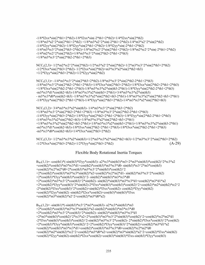
235

-1/8*I2xx*sin(2*th1+2*th2)-1/8*I2xx*sin(-2*th1+2*th2)+1/4*I2xx*sin(2*th2) +1/8*m3*a2^2*sin(2*th1+2*th2) +1/8*m3*a2^2*sin(-2*th1+2*th2)-1/4*m3*a2^2*sin(2*th2) -1/4*I2yy*sin(2*th2)+1/8*I2yy*sin(2*th1+2*th2)+1/8*I2yy*sin(-2*th1+2*th2) -1/4*m3*rc3^2*sin(2*th3+2*th2)+1/8*m2*rc2^2*sin(2*th1+2*th2)+1/8*m2*rc2^2*sin(-2*th1+2*th2) -1/4*m2*rc2^2*sin(2*th2)+1/8*m3*rc3^2*sin(2*th2+2*th1+2*th3) +1/8*m3*rc3^2*sin(2*th2-2*th1+2*th3) NCCτ(2,3)= 1/2*m2*rc2^2*sin(2*th2)+1/2*m3*a2^2*sin(2*th2)+1/2*m3*rc3^2*sin(2*th3+2*th2) -1/2*I3xx*sin(2*th3+2*th2)- 1/2*I2xx*sin(2*th2)+m3*rc3*a2*sin(2*th2+th3) +1/2*I3yy*sin(2*th3+2*th2)+1/2*I2yy*sin(2*th2) NCCτ(3,1)= -1/4*m3*rc3^2*sin(2*th3+2*th2)-1/8*m3*rc3^2*sin(2*th2-2*th1+2*th3) -1/8*m3*rc3^2*sin(2*th2+2*th1+2*th3)+1/4*I3xx*sin(2*th3+2*th2)+1/8*I3xx*sin(2*th2+2*th1+2*th3) +1/8*I3xx*sin(2*th2-2*th1+2*th3)-1/8*m3*rc3*a2*sin(th3-2*th1)-1/8*I3yy*sin(2*th2-2*th1+2*th3) -m3*rc3*d1*cos(th2+th3)-1/8*m3*rc3*a2*sin(th3+2*th1)+3/4*m3*rc3*a2*sin(th3) - m3*rc3*d0*cos(th2+th3) -1/8*m3*rc3*a2*sin(2*th2+th3-2*th1)-1/8*m3*rc3*a2*sin(2*th2+th3+2*th1) -1/8*I3yy*sin(2*th2+2*th1+2*th3)-1/4*I3yy*sin(2*th3+2*th2)-1/4*m3*rc3*a2*sin(2*th2+th3) NCCτ(3,2)= 3/4*m3*rc3*a2*sin(th3)- 1/4*m3*rc3^2*sin(2*th3+2*th2) +1/8*m3*rc3^2*sin(2*th2+2*th1+2*th3) +1/8*m3*rc3^2*sin(2*th2-2*th1+2*th3) -1/4*I3yy*sin(2*th3+2*th2)+1/8*I3yy*sin(2*th2+2*th1+2*th3)+1/8*I3yy*sin(2*th2-2*th1+2*th3) -1/4*m3*rc3*a2*sin(2*th2+th3)+1/8*m3*rc3*a2*sin(2*th2+th3+2*th1) +1/8*m3*rc3*a2*sin(2*th2+th3-2*th1)+1/8*m3*rc3*a2*sin(th3+2*th1)+1/8*m3*rc3*a2*sin(th3-2*th1) -m3*rc3*d1*cos(th2+th3)-1/8*I3xx*sin(2*th2+2*th1+2*th3)-1/8*I3xx*sin(2*th2-2*th1+2*th3) -m3*rc3*d0*cos(th2+th3)+1/4*I3xx*sin(2*th3+2*th2) NCCτ(3,3)= 1/2*m3*rc3*a2*sin(th3)+1/2*m3*rc3*a2*sin(2*th2+th3)+1/2*m3*rc3^2*sin(2*th3+2*th2) -1/2*I3xx*sin(2*th3+2*th2)+1/2*I3yy*sin(2*th3+2*th2) (A-29)

Flexible Body Rotational Inertia Torques

BWτ(1,1)= -cos(th1)*(-sin(th3)*I3yy*cos(th3)- a2*rc3*sin(th3)*m3+2*m3*sin(th3)*cos(th2)^2*rc3*a2 +cos(th2)*cos(th3)*m3*rc3*d1+cos(th2)*cos(th3)*m3*rc3*d0- sin(th3)*rc3^2*m3*cos(th3) +cos(th2)*rc2*m2*d0+2*cos(th3)*m3*rc3^2*sin(th3)*cos(th2)^2 +2*cos(th2)*cos(th3)*m3*rc3*sin(th2)*a2+cos(th2)*rc2*m2*d1- sin(th2)*m3*rc3^2*cos(th2) +2*cos(th3)*I3yy*sin(th3)*cos(th2)^2- sin(th2)*sin(th3)*m3*rc3*d0 +2*cos(th2)*m3*rc3^2*cos(th3)^2*sin(th2)- sin(th2)*sin(th3)*m3*rc3*d1+cos(th2)*m3*d1*a2 +2*cos(th2)*I3yy*cos(th3)^2*sin(th2)-2*I3xx*sin(th3)*cos(th3)*cos(th2)^2+cos(th2)*m2*sin(th2)*rc2^2 -2*sin(th2)*I3xx*cos(th3)^2*cos(th2)+sin(th2)*I3xx*cos(th2)- cos(th2)*I3yy*sin(th2) +cos(th2)*I2yy*sin(th2) -sin(th2)*I2xx*cos(th2)+cos(th3)*sin(th3)*I3xx +cos(th2)*m3*sin(th2)*a2^2+cos(th2)*m3*d0*a2) BWτ(1,2)= -sin(th1)*(-sin(th3)*rc3^2*m3*cos(th3)- a2*rc3*sin(th3)*m3 +2*cos(th2)*cos(th3)*m3*rc3*sin(th2)*a2-sin(th2)*sin(th3)*m3*rc3*d0 +2*cos(th2)*m3*rc3^2*cos(th3)^2*sin(th2)- sin(th2)*sin(th3)*m3*rc3*d1 +2*m3*sin(th3)*cos(th2)^2*rc3*a2+2*cos(th3)*m3*rc3^2*sin(th3)*cos(th2)^2+cos(th2)*rc2*m2*d1 -2*I3xx*sin(th3)*cos(th3)*cos(th2)^2-sin(th2)*m3*rc3^2*cos(th2)- 2*sin(th2)*I3xx*cos(th3)^2*cos(th2) +2*cos(th3)*I3yy*sin(th3)*cos(th2)^2+2*cos(th2)*I3yy*cos(th3)^2*sin(th2)+cos(th2)*m3*d1*a2 +cos(th2)*cos(th3)*m3*rc3*d1+cos(th2)*cos(th3)*m3*rc3*d0+cos(th2)*rc2*m2*d0 +cos(th2)*m2*sin(th2)*rc2^2+cos(th2)*m3*d0*a2+cos(th2)*m3*sin(th2)*a2^2+cos(th2)*I3xx*sin(th2) +cos(th2)*I2yy*sin(th2)-sin(th2)*I2xx*cos(th2)+cos(th3)*sin(th3)*I3xx-sin(th3)*I3yy*cos(th3)

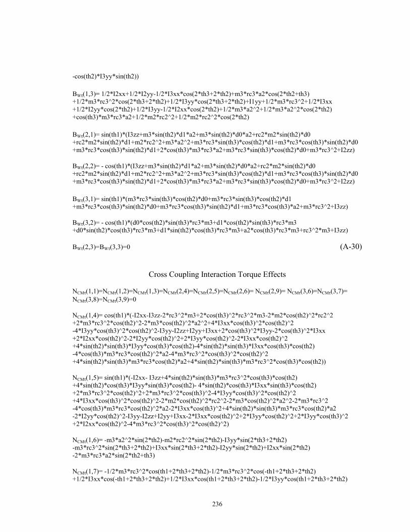
236

-cos(th2)*I3yy*sin(th2)) BWτ(1,3)= 1/2*I2xx+1/2*I2yy-1/2*I3xx*cos(2*th3+2*th2)+m3*rc3*a2*cos(2*th2+th3) +1/2*m3*rc3^2*cos(2*th3+2*th2)+1/2*I3yy*cos(2*th3+2*th2)+I1yy+1/2*m3*rc3^2+1/2*I3xx +1/2*I2yy*cos(2*th2)+1/2*I3yy-1/2*I2xx*cos(2*th2)+1/2*m3*a2^2+1/2*m3*a2^2*cos(2*th2) +cos(th3)*m3*rc3*a2+1/2*m2*rc2^2+1/2*m2*rc2^2*cos(2*th2) BWτ(2,1)= sin(th1)*(I3zz+m3*sin(th2)*d1*a2+m3*sin(th2)*d0*a2+rc2*m2*sin(th2)*d0 +rc2*m2*sin(th2)*d1+m2*rc2^2+m3*a2^2+m3*rc3*sin(th3)*cos(th2)*d1+m3*rc3*cos(th3)*sin(th2)*d0 +m3*rc3*cos(th3)*sin(th2)*d1+2*cos(th3)*m3*rc3*a2+m3*rc3*sin(th3)*cos(th2)*d0+m3*rc3^2+I2zz) BWτ(2,2)= - cos(th1)*(I3zz+m3*sin(th2)*d1*a2+m3*sin(th2)*d0*a2+rc2*m2*sin(th2)*d0 +rc2*m2*sin(th2)*d1+m2*rc2^2+m3*a2^2+m3*rc3*sin(th3)*cos(th2)*d1+m3*rc3*cos(th3)*sin(th2)*d0 +m3*rc3*cos(th3)*sin(th2)*d1+2*cos(th3)*m3*rc3*a2+m3*rc3*sin(th3)*cos(th2)*d0+m3*rc3^2+I2zz) BWτ(3,1)= sin(th1)*(m3*rc3*sin(th3)*cos(th2)*d0+m3*rc3*sin(th3)*cos(th2)*d1 +m3*rc3*cos(th3)*sin(th2)*d0+m3*rc3*cos(th3)*sin(th2)*d1+m3*rc3*cos(th3)*a2+m3*rc3^2+I3zz) BWτ(3,2)= - cos(th1)*(d0*cos(th2)*sin(th3)*rc3*m3+d1*cos(th2)*sin(th3)*rc3*m3 +d0*sin(th2)*cos(th3)*rc3*m3+d1*sin(th2)*cos(th3)*rc3*m3+a2*cos(th3)*rc3*m3+rc3^2*m3+I3zz) BWτ(2,3)=BWτ(3,3)=0 (A-30)

Cross Coupling Interaction Torque Effects NCMτ(1,1)=NCMτ(1,2)=NCMτ(1,3)=NCMτ(2,4)=NCMτ(2,5)=NCMτ(2,6)= NCMτ(2,9)= NCMτ(3,6)=NCMτ(3,7)= NCMτ(3,8)=NCMτ(3,9)=0 NCMτ(1,4)= cos(th1)*(-I2xx-I3zz-2*rc3^2*m3+2*cos(th3)^2*rc3^2*m3-2*m2*cos(th2)^2*rc2^2 +2*m3*rc3^2*cos(th2)^2-2*m3*cos(th2)^2*a2^2+4*I3xx*cos(th3)^2*cos(th2)^2 -4*I3yy*cos(th3)^2*cos(th2)^2-I3yy-I2zz+I2yy+I3xx+2*cos(th3)^2*I3yy-2*cos(th3)^2*I3xx +2*I2xx*cos(th2)^2-2*I2yy*cos(th2)^2+2*I3yy*cos(th2)^2-2*I3xx*cos(th2)^2 +4*sin(th2)*sin(th3)*I3yy*cos(th3)*cos(th2)-4*sin(th2)*sin(th3)*I3xx*cos(th3)*cos(th2) -4*cos(th3)*m3*rc3*cos(th2)^2*a2-4*m3*rc3^2*cos(th3)^2*cos(th2)^2 +4*sin(th2)*sin(th3)*m3*rc3*cos(th2)*a2+4*sin(th2)*sin(th3)*m3*rc3^2*cos(th3)*cos(th2)) NCMτ(1,5)= sin(th1)*(-I2xx- I3zz+4*sin(th2)*sin(th3)*m3*rc3^2*cos(th3)*cos(th2) +4*sin(th2)*cos(th3)*I3yy*sin(th3)*cos(th2)- 4*sin(th2)*cos(th3)*I3xx*sin(th3)*cos(th2) +2*m3*rc3^2*cos(th2)^2+2*m3*rc3^2*cos(th3)^2-4*I3yy*cos(th3)^2*cos(th2)^2 +4*I3xx*cos(th3)^2*cos(th2)^2-2*m2*cos(th2)^2*rc2^2-2*m3*cos(th2)^2*a2^2-2*m3*rc3^2 -4*cos(th3)*m3*rc3*cos(th2)^2*a2-2*I3xx*cos(th3)^2+4*sin(th2)*sin(th3)*m3*rc3*cos(th2)*a2 -2*I2yy*cos(th2)^2-I3yy-I2zz+I2yy+I3xx-2*I3xx*cos(th2)^2+2*I3yy*cos(th2)^2+2*I3yy*cos(th3)^2 +2*I2xx*cos(th2)^2-4*m3*rc3^2*cos(th3)^2*cos(th2)^2) NCMτ(1,6)= -m3*a2^2*sin(2*th2)-m2*rc2^2*sin(2*th2)-I3yy*sin(2*th3+2*th2) -m3*rc3^2*sin(2*th3+2*th2)+I3xx*sin(2*th3+2*th2)-I2yy*sin(2*th2)+I2xx*sin(2*th2) -2*m3*rc3*a2*sin(2*th2+th3) NCMτ(1,7)= -1/2*m3*rc3^2*cos(th1+2*th3+2*th2)-1/2*m3*rc3^2*cos(-th1+2*th3+2*th2) +1/2*I3xx*cos(-th1+2*th3+2*th2)+1/2*I3xx*cos(th1+2*th3+2*th2)-1/2*I3yy*cos(th1+2*th3+2*th2)

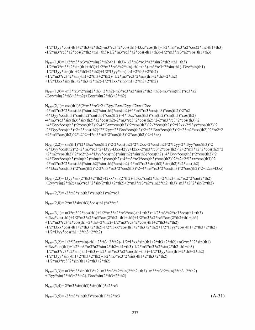
237

-1/2*I3yy*cos(-th1+2*th3+2*th2)-m3*rc3^2*cos(th1)-I3zz*cos(th1)-1/2*m3*rc3*a2*cos(2*th2-th1+th3) -1/2*m3*rc3*a2*cos(2*th2+th1+th3)-1/2*m3*rc3*a2*cos(-th1+th3)-1/2*m3*rc3*a2*cos(th1+th3) NCMτ(1,8)= 1/2*m3*rc3*a2*sin(2*th2-th1+th3)-1/2*m3*rc3*a2*sin(2*th2+th1+th3) -1/2*m3*rc3*a2*sin(th1+th3)+1/2*m3*rc3*a2*sin(-th1+th3)-m3*rc3^2*sin(th1)-I3zz*sin(th1) -1/2*I3yy*sin(th1+2*th3+2*th2)+1/2*I3yy*sin(-th1+2*th3+2*th2) +1/2*m3*rc3^2*sin(-th1+2*th3+2*th2)- 1/2*m3*rc3^2*sin(th1+2*th3+2*th2) +1/2*I3xx*sin(th1+2*th3+2*th2)-1/2*I3xx*sin(-th1+2*th3+2*th2) NCMτ(1,9)= -m3*rc3^2*sin(2*th3+2*th2)-m3*rc3*a2*sin(2*th2+th3)-m3*sin(th3)*rc3*a2 -I3yy*sin(2*th3+2*th2)+I3xx*sin(2*th3+2*th2) NCMτ(2,1)= cos(th1)*(2*m3*rc3^2+I3yy-I3xx-I2yy+I2xx+I2zz -4*m3*rc3^2*cos(th3)*sin(th2)*sin(th3)*cos(th2)+4*m3*rc3*cos(th3)*cos(th2)^2*a2 -4*I3yy*cos(th3)*sin(th2)*sin(th3)*cos(th2)+4*I3xx*cos(th3)*sin(th2)*sin(th3)*cos(th2) -4*m3*rc3*sin(th3)*sin(th2)*a2*cos(th2)-2*m3*rc3^2*cos(th2)^2-2*m3*rc3^2*cos(th3)^2 +4*I3yy*cos(th3)^2*cos(th2)^2-4*I3xx*cos(th3)^2*cos(th2)^2-2*cos(th2)^2*I2xx-2*I3yy*cos(th2)^2 -2*I3yy*cos(th3)^2+2*cos(th2)^2*I2yy+2*I3xx*cos(th2)^2+2*I3xx*cos(th3)^2+2*m2*cos(th2)^2*rc2^2 +2*m3*cos(th2)^2*a2^2+4*m3*rc3^2*cos(th3)^2*cos(th2)^2+I3zz) NCMτ(2,2)= sin(th1)*(2*I3xx*cos(th2)^2-2*cos(th2)^2*I2xx+2*cos(th2)^2*I2yy-2*I3yy*cos(th3)^2 -2*I3yy*cos(th2)^2+2*m3*rc3^2+I3yy-I3xx-I2yy+I2xx-2*m3*rc3^2*cos(th2)^2+2*m3*a2^2*cos(th2)^2 +2*m2*cos(th2)^2*rc2^2-4*I3yy*cos(th3)*sin(th2)*sin(th3)*cos(th2)+4*I3yy*cos(th3)^2*cos(th2)^2 +4*I3xx*cos(th3)*sin(th2)*sin(th3)*cos(th2)+4*m3*rc3*cos(th3)*cos(th2)^2*a2+2*I3xx*cos(th3)^2 -4*m3*rc3^2*cos(th3)*sin(th2)*sin(th3)*cos(th2)-4*m3*rc3*sin(th3)*sin(th2)*a2*cos(th2) -4*I3xx*cos(th3)^2*cos(th2)^2-2*m3*rc3^2*cos(th3)^2+4*m3*rc3^2*cos(th3)^2*cos(th2)^2+I2zz+I3zz) NCMτ(2,3)= I3yy*sin(2*th3+2*th2)-I2xx*sin(2*th2)- I3xx*sin(2*th3+2*th2)+m2*rc2^2*sin(2*th2) +I2yy*sin(2*th2)+m3*rc3^2*sin(2*th3+2*th2)+2*m3*rc3*a2*sin(2*th2+th3)+m3*a2^2*sin(2*th2) NCMτ(2,7)= -2*m3*sin(th3)*sin(th1)*a2*rc3 NCMτ(2,8)= 2*m3*sin(th3)*cos(th1)*a2*rc3 NCMτ(3,1)= m3*rc3^2*cos(th1)+1/2*m3*a2*rc3*cos(-th1+th3)+1/2*m3*a2*rc3*cos(th1+th3) +I3zz*cos(th1)+1/2*m3*a2*rc3*cos(2*th2- th1+th3)+1/2*m3*a2*rc3*cos(2*th2+th1+th3) +1/2*m3*rc3^2*cos(th1+2*th3+2*th2)+1/2*m3*rc3^2*cos(-th1+2*th3+2*th2) -1/2*I3xx*cos(-th1+2*th3+2*th2)-1/2*I3xx*cos(th1+2*th3+2*th2)+1/2*I3yy*cos(-th1+2*th3+2*th2) +1/2*I3yy*cos(th1+2*th3+2*th2) NCMτ(3,2)= 1/2*I3xx*sin(-th1+2*th3+2*th2)- 1/2*I3xx*sin(th1+2*th3+2*th2)+m3*rc3^2*sin(th1) +I3zz*sin(th1)+1/2*m3*rc3*a2*sin(2*th2+th1+th3)-1/2*m3*rc3*a2*sin(2*th2-th1+th3) -1/2*m3*rc3*a2*sin(-th1+th3)+1/2*m3*rc3*a2*sin(th1+th3)+1/2*I3yy*sin(th1+2*th3+2*th2) -1/2*I3yy*sin(-th1+2*th3+2*th2)-1/2*m3*rc3^2*sin(-th1+2*th3+2*th2) +1/2*m3*rc3^2*sin(th1+2*th3+2*th2) NCMτ(3,3)= m3*rc3*sin(th3)*a2+m3*rc3*a2*sin(2*th2+th3)+m3*rc3^2*sin(2*th3+2*th2) +I3yy*sin(2*th3+2*th2)-I3xx*sin(2*th3+2*th2) NCMτ(3,4)= 2*m3*sin(th3)*sin(th1)*a2*rc3 NCMτ(3,5)= -2*m3*sin(th3)*cos(th1)*a2*rc3 (A-31)

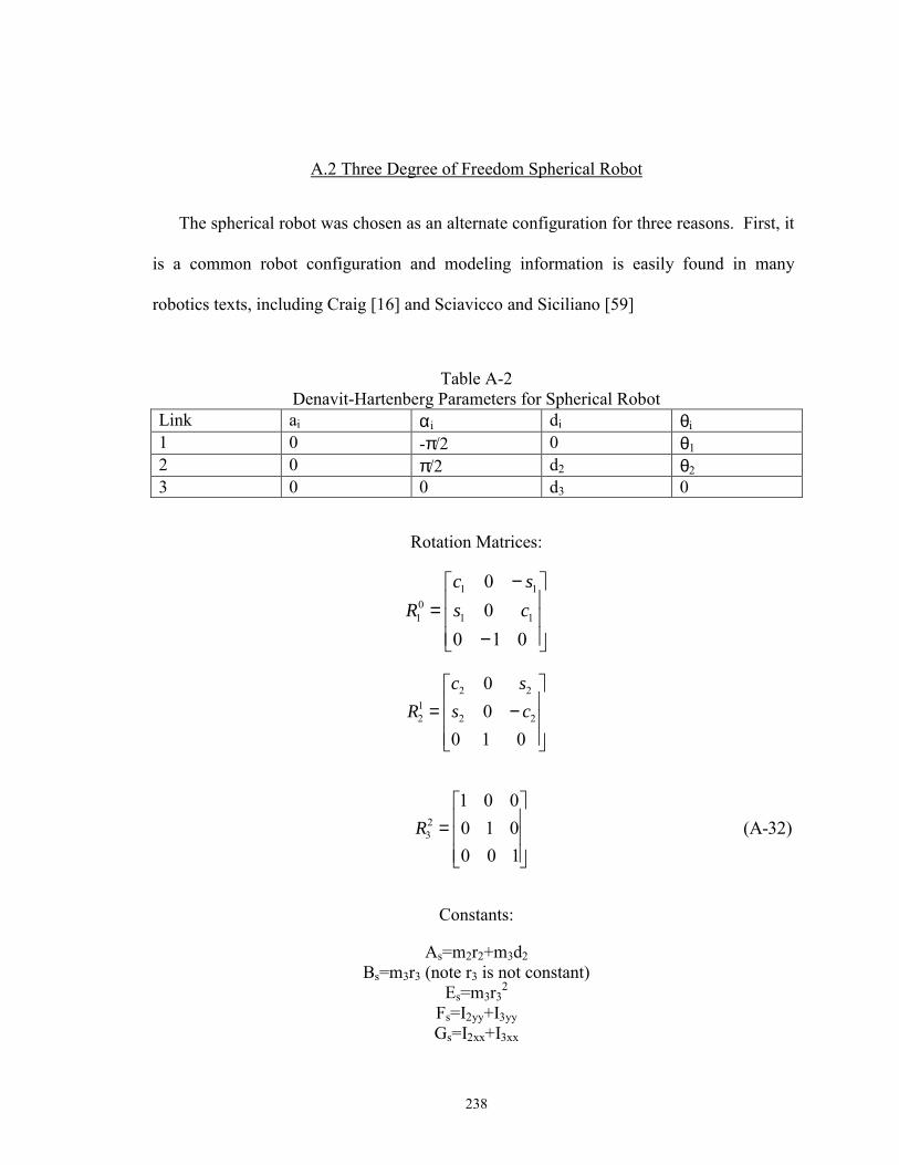
238

A.2 Three Degree of Freedom Spherical Robot

The spherical robot was chosen as an alternate configuration for three reasons. First, it

is a common robot configuration and modeling information is easily found in many

robotics texts, including Craig [16] and Sciavicco and Siciliano [59]

Table A-2 Denavit-Hartenberg Parameters for Spherical Robot

Link ai αi di θi 1 0 -π/2 0 θ1 2 0 π/2 d2 θ2 3 0 0 d3 0

Rotation Matrices:

1 101 1 1

00

0 1 0

c sR s c

− = −

2 212 2 2

0 0

0 1 0

c sR s c

= −

23

1 0 00 1 0 (A-32)0 0 1

R =

Constants:

As=m2r2+m3d2 Bs=m3r3 (note r3 is not constant)

Es=m3r32

Fs=I2yy+I3yy Gs=I2xx+I3xx

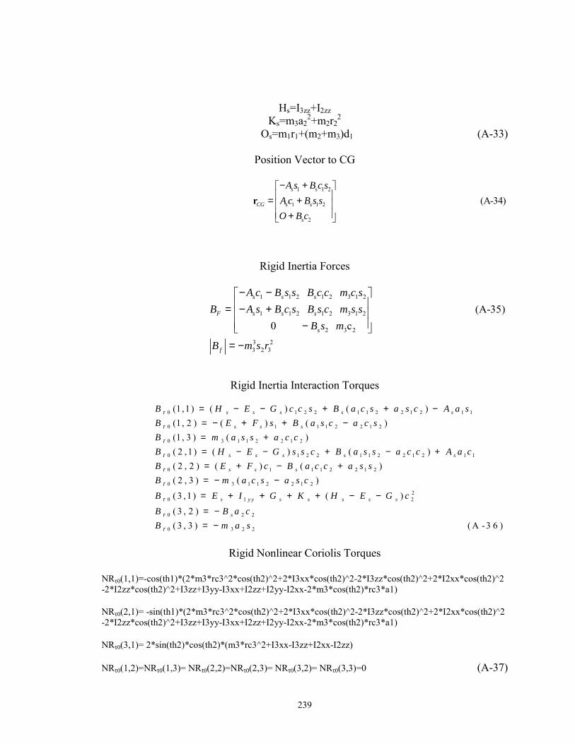
239

Hs=I3zz+I2zz Ks=m3a2

2+m2r22

Os=m1r1+(m2+m3)d1 (A-33)

Position Vector to CG

1 1 2

1 1 2

2

(A-34)s s

CG s s

s

A s B c sA c B s sO B c

− + = + +

r

Rigid Inertia Forces

1 1 2 1 2 3 1 2

1 1 2 1 2 3 1 2

2 3 2

3 23 2 3

(A-35) 0 c

s s s

F s s s

s

f

A c B s s B c c m c sB A s B c s B s c m s s

B s m

B m s r

− − = − + −

= −

Rigid Inertia Interaction Torques

0 1 2 2 1 1 2 2 1 2 1 1

0 1 1 1 2 2 1 2

0 3 1 1 2 2 1 2

0 1 2 2 1 1 2 2 1 2 1 1

0 1 1 1 2 2 1 2

(1 ,1 ) ( ) ( )(1 , 2 ) ( ) ( )(1 , 3 ) ( )( 2 ,1 ) ( ) ( )( 2 , 2 ) ( ) ( )

s s s s s

s s s

s s s s s

s s s

B H E G c c s B a c s a s c A a sB E F s B a s c a c sB m a s s a c cB H E G s s c B a s s a c c A a cB E F c B a c c a s sB

τ

τ

τ

τ

τ

= − − + + −= − + + −= += − − + − += + − +

0 3 1 1 2 2 1 2

20 1 2

0 2 2

0 3 2 2

( 2 , 3 ) ( )

( 3 ,1 ) ( )

( 3 , 2 )( 3 , 3 ) ( A - 3 6 )

s y y s s s s s

s

m a c s a s cB E I G K H E G cB B a cB m a s

τ

τ

τ

τ

= − −

= + + + + − −

= −= −

Rigid Nonlinear Coriolis Torques

NRτ0(1,1)=-cos(th1)*(2*m3*rc3^2*cos(th2)^2+2*I3xx*cos(th2)^2-2*I3zz*cos(th2)^2+2*I2xx*cos(th2)^2 -2*I2zz*cos(th2)^2+I3zz+I3yy-I3xx+I2zz+I2yy-I2xx-2*m3*cos(th2)*rc3*a1) NRτ0(2,1)= -sin(th1)*(2*m3*rc3^2*cos(th2)^2+2*I3xx*cos(th2)^2-2*I3zz*cos(th2)^2+2*I2xx*cos(th2)^2 -2*I2zz*cos(th2)^2+I3zz+I3yy-I3xx+I2zz+I2yy-I2xx-2*m3*cos(th2)*rc3*a1) NRτ0(3,1)= 2*sin(th2)*cos(th2)*(m3*rc3^2+I3xx-I3zz+I2xx-I2zz) NRτ0(1,2)=NRτ0(1,3)= NRτ0(2,2)=NRτ0(2,3)= NRτ0(3,2)= NRτ0(3,3)=0 (A-37)

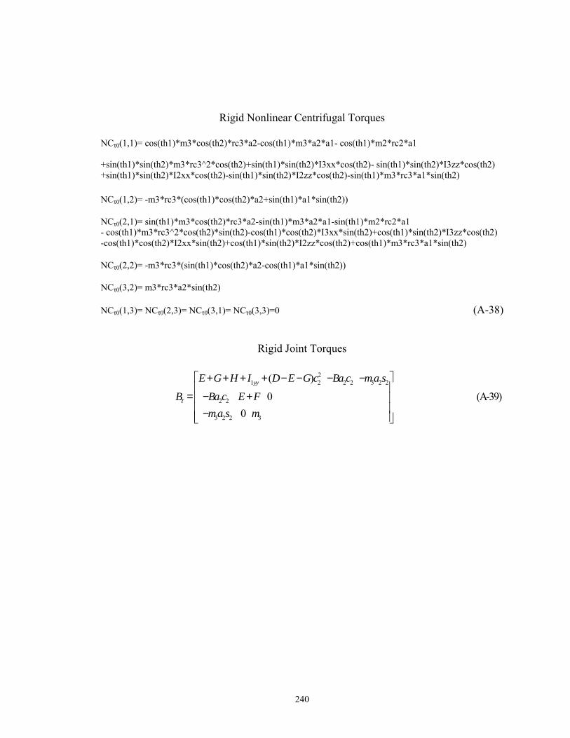
240

Rigid Nonlinear Centrifugal Torques

NCτ0(1,1)= cos(th1)*m3*cos(th2)*rc3*a2-cos(th1)*m3*a2*a1- cos(th1)*m2*rc2*a1 +sin(th1)*sin(th2)*m3*rc3^2*cos(th2)+sin(th1)*sin(th2)*I3xx*cos(th2)- sin(th1)*sin(th2)*I3zz*cos(th2) +sin(th1)*sin(th2)*I2xx*cos(th2)-sin(th1)*sin(th2)*I2zz*cos(th2)-sin(th1)*m3*rc3*a1*sin(th2) NCτ0(1,2)= -m3*rc3*(cos(th1)*cos(th2)*a2+sin(th1)*a1*sin(th2)) NCτ0(2,1)= sin(th1)*m3*cos(th2)*rc3*a2-sin(th1)*m3*a2*a1-sin(th1)*m2*rc2*a1 - cos(th1)*m3*rc3^2*cos(th2)*sin(th2)-cos(th1)*cos(th2)*I3xx*sin(th2)+cos(th1)*sin(th2)*I3zz*cos(th2) -cos(th1)*cos(th2)*I2xx*sin(th2)+cos(th1)*sin(th2)*I2zz*cos(th2)+cos(th1)*m3*rc3*a1*sin(th2) NCτ0(2,2)= -m3*rc3*(sin(th1)*cos(th2)*a2-cos(th1)*a1*sin(th2)) NCτ0(3,2)= m3*rc3*a2*sin(th2) NCτ0(1,3)= NCτ0(2,3)= NCτ0(3,1)= NCτ0(3,3)=0 (A-38)

Rigid Joint Torques

21 2 2 2 3 2 2

2 2

3 2 2 3

( )

0 (A-39)0

yyE G H I D E G c Ba c ma sB Ba c E F

ma s mτ

+ + + + − − − −

= − + −

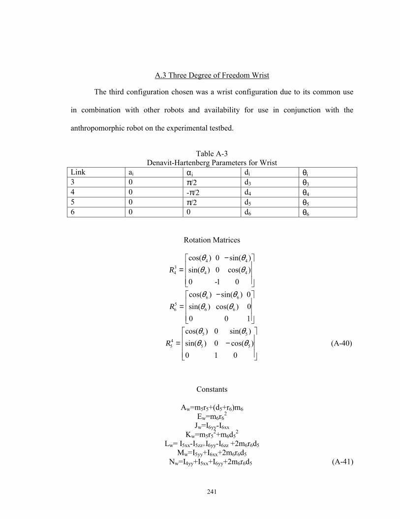
241

A.3 Three Degree of Freedom Wrist

The third configuration chosen was a wrist configuration due to its common use

in combination with other robots and availability for use in conjunction with the

anthropomorphic robot on the experimental testbed.

Table A-3

Denavit-Hartenberg Parameters for Wrist Link ai αi di θi 3 0 π/2 d3 θ3 4 0 -π/2 d4 θ4 5 0 π/2 d5 θ5 6 0 0 d6 θ6

Rotation Matrices

4 434 4 4

cos( ) 0 sin( )sin( ) 0 cos( )0 -1 0

Rθ θθ θ

− =

6 656 6 6

cos( ) sin( ) 0sin( ) cos( ) 00 0 1

Rθ θθ θ

− =

5 545 5 5

cos( ) 0 sin( )sin( ) 0 cos( ) (A-40)0 1 0

Rθ θθ θ

= −

Constants

Aw=m5r5+(d5+r6)m6 Ew=m6r6

2

Jw=I6yy-I6xx Kw=m5r5

2+m6d52

Lw= I5xx-I5zz+I6yy-I6zz +2m6r6d5 Mw=I5yy+I6xx+2m6r6d5

Nw=I4yy+I5xx+I6yy+2m6r6d5 (A-41)

242

Position Vector to CG

6 4 5

6 4 5

3 5 3

cos( )sin( )sin( )sin( ) (A-42)(cos( ) )

CG

mmm r

θ θθ θθ

= −

r

Rigid Inertia Forces

4 5 4 5

4 5 4 5

5

0 0 (A-43) 0 0

w w

f w w

w

A s s A c cB A c s A s c

A s

− = −

Rigid Inertia Interaction Torques

{ }

{ }

0 5 4 5 4 4 6 4 6 4 5 6

0 4 4 4 5 6 4 6 4 5 6

0 6 4 5

0 5 4 5 4 4 6 4 6 4 5 6

0 4 4 4 5

(1,1) ( ) ( )(1,2) ( ) ( )(1,3)(2,1) ( ) ( )(2,2) ( )

w w w w w

w w w w w

zz

w w w w w

w w w w

B s K E L c c A d c J c s s c c cB M E L s A d s c J c s c c c sB I c sB s K E L s c A d s J c c s s c cB M E L c A d c c J

τ

τ

τ

τ

τ

= − + + + + −= − + + − − +== − + + − + −= + + + + 6 4 6 4 5 6

0 6 4 52 2 2

0 5 5 6

0 5 6 6

0 6 5

( )(2,3)(3,1) ( )(3,2)(3,3) (A-44)

w

zz

w w w w

w

zz

c c c s c sB I s sB s K E L J s cB J s s cB I c

τ

τ

τ

τ

−=

= − + + −==

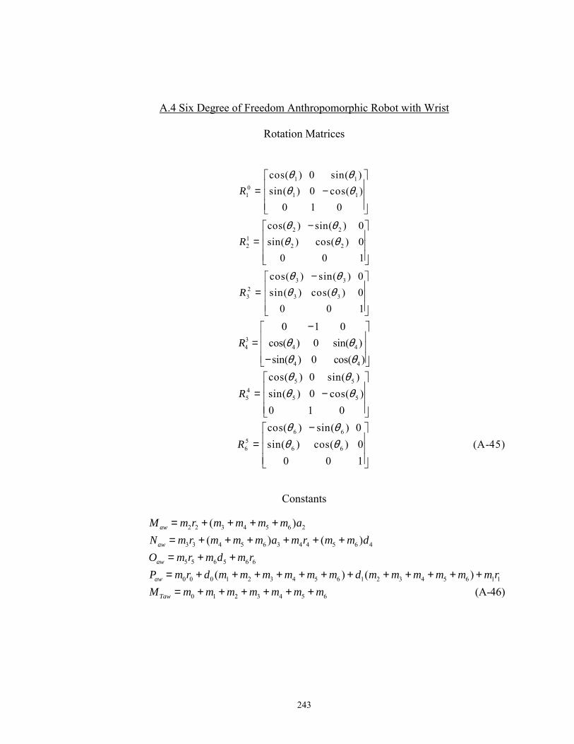
243

A.4 Six Degree of Freedom Anthropomorphic Robot with Wrist

Rotation Matrices

1 10

1 1 1

cos( ) 0 sin( )sin( ) 0 cos( ) 0 1 0

Rθ θθ θ

= −

2 212 2 2

cos( ) sin( ) 0sin( ) cos( ) 0 0 0 1

Rθ θθ θ

− =

3 323 3 3

cos( ) sin( ) 0sin( ) cos( ) 0 0 0 1

Rθ θθ θ

− =

34 4 4

4 4

0 1 0cos( ) 0 sin( )sin( ) 0 cos( )

R θ θθ θ

− = −

5 545 5 5

cos( ) 0 sin( )sin( ) 0 cos( )0 1 0

Rθ θθ θ

= −

6 656 6 6

cos( ) sin( ) 0sin( ) cos( ) 0 (A-45) 0 0 1

Rθ θθ θ

− =

Constants

2 2 3 4 5 6 2

3 3 4 5 6 3 4 4 5 6 4

5 5 6 5 6 6

0 0 0 1 2 3 4 5 6 1 2 3 4 5 6 1 1

0 1 2 3 4 5 6

( )( ) ( )

( ) ( )

aw

aw

aw

aw

Taw

M m r m m m m aN m r m m m a m r m m dO m r m d m rP m r d m m m m m m d m m m m m m rM m m m m m m m

= + + + += + + + + + += + += + + + + + + + + + + + += + + + + + + (A-46)

244

Position Vector To CG

1 2 23 5 23 4 5 23 1 4 5

1 2 23 5 23 4 5 23 1 4 5

2 23 5 23 4 5 23

( )1 ( ) (A-47)

aw aw aw aw

CG aw aw aw awTaw

aw aw aw aw aw

c M c N c O c c O c s s Os s ss M c N c O c c O c s s Oc s s

MP M s N s O c s O c s c

+ + − − = + + − + + + + +

r

Rigid Interaction Forces

Bf=

1 2 23 5 23 4 5 1 4 5 1 2 23 5 23 4 5 1 4 5

1 2 23 5 23 4 5 1 2 23 5 23 4 5 2 5 23 4 5

{ ( ) } { ( ) } 0 { ( ) } { ( ) } ( )

s Mc c N Oc Os c s Oc s s c Mc c N Oc Os c s Os s sc Ms s N Oc Oc c s s Ms s N Oc Oc c s c M N Oc Os c s

− + + + − + + − −− + + + − + + + + + −

1 23 5 23 4 5 1 23 5 23 4 5 23 5 23 4 5

5 1 23 4 1 4 5 1 23 4 1 4

{ ( ) } { ( ) } ( ) ( ) ( )

c s N Oc Oc c s s s N Oc Oc c s c N Oc Os c sOs c s s s c Os s s s cc

− + + − + + + −− + 23 4 5

1 23 5 23 4 5 1 4 5 1 23 5 23 4 5 1 4 5 23 4 5 5 23

{ ( ) } { ( ) } ( ) 0

Oc s sO c c s s c c s s c O s c s s c c c s c O c c c s s

−− + + − + + −

0 0

T

(A-48)

Rigid Interaction Coriolis Forces

1 2 23 5 23 4 5 1 2 23 5 23 4 5

1 23 5 23 4 5 1 23 5 23 4 5

1 *

2 { ( ) } -2 { ( ) } 0 2 { ( ) } -2 { ( ) }

fTaw

aw aw aw aw aw aw aw aw

aw aw aw aw aw aw

NRM

s M s s N O c O c c s c M s s N O c O c c ss s N O c O c c s c s N O c O c c s

=

+ + + + + ++ + + +

5 1 23 4 1 4 5 1 23 4 1 4

1 5 23 23 4 5 1 4 5 1 23 5 23 4 5 1 4 5

0 -2 { } -2 { } 0 2 { ( ) } 2 { ( ) }

aw aw

aw aw

O s ss s cc O s cs s scO s s c s c c cs c O c c s s c s s s c

+ − ++ − − + +

1 23

0 0 0 0 2 { (c c N− 5 23 4 5 1 23 5 23 4 5 23 5 23 4 5

1 23 4 5 1 23 4 5

) } 2 { ( ) } -2{ ( ) } 2 2

aw aw aw aw aw aw aw aw aw

aw aw

O c O s c s s c N O c O s c s s N O c O c c sO cc s s O sc s s

+ + − + + + +

23 4 5

1 23 5 23 4 5 1 23 5 23 4 5 23 5 23 4 5

2 -2 { } -2 { } -2 { } 0

aw

aw aw aw

O s s sO c s s c c c O s s s c c c O c s s c c− + − + +

1 23 4 5 1 23 4 5

0 0 2 2 aw awO cc s s O sc s s 23 4 5

1 23 5 23 4 5 1 23 5 23 4 5 23 5 23 4 5

2 -2 { } -2 { } -2 { } 0

aw

aw aw aw

O s s sO c s s c c c O s s s c c c O c s s c c− + − + +

5 1 23 4 1 4 5 1 23 4 1 4

0 0 -2 { } 2 { } aw awO c cs s sc O c ss s cc− + + 23 4 5 -2

T

awO c s c

(A-49)

245

Rigid Interaction Centrifugal Forces

1 4 5 2 23 5 23 1 4 5

1 2 23 5 23 4 5

1 23 5 23 4 5

1 23 4 1 4

1(1,1) * { ( ) }

1(1,2) * { ( ) }

1(1,3) * { ( ) }

1(1,4) *{ ( )}

(1,5)

f aw aw aw aw awTaw

f aw aw aw awTaw

f aw aw awTaw

f awTaw

f

NC cc s M c c N O c O s O ss sM

NC c M c c N O c O s c sM

NC c c N O c O s c sM

NC O cs c ssM

NC

= − − + + +

= − − + +

= − + +

= +

= 1 23 4 5 5 23 1 4 5

1 2 23 5 23 4 5 1 4 5

1 2 23 5 23 4 5

23 5 23 4 5

1 *{ [ ( ] }

(1,6) 0

1(2,1) *{ [ ( ) ]

1(2,2) *{ [ ( ) ]

1(2,3) *{ ( )

awTaw

f

f aw aw aw awTaw

f aw aw aw awTaw

f aw aw awTaw

O c s c s c c ss sM

NC

NC s M c c N O c O s c s Ocs sM

NC s M c c N O c O s c sM

NC c N O c O s c sM

− +

=

= − − + + −

= − − + +

= − + +

5 1 23 4 1 4

1 23 4 5 5 23 1 4 5

2 23 5 23 4 5

23 5 23 4 5

}

1(2,4) *{ ( )

1(2,5) *{ [ ( ) ]}

(2,6) 0

(3,1) 0

1(3,2) *{ [ ( ) }

1(3,3) *{ ( ) }

(3

f awTaw

f awTaw

f

f

f aw aw aw awTaw

f aw aw awTaw

f

NC O s ss c csM

NC O s s c s c c cs sM

NCNC

NC M s s N O c O c c sM

NC s N O c O c c sM

NC

= −

= − −

=

=

= − + + +

= − + +

23 4 5

5 23 23 4 5

1,4) *{ }

1(3,5) *{ ( }

awTaw

f awTaw

O c c sM

NC O c s c c sM

= −

= − +

(A-50)

246

REFERENCES

[1] ATI Industrial Automation. Installation and Operations Manual for Stand-Alone F/T Sensor Systems: Intelligent MultiAxis Force/Torque Sensor System. Manual PN 9610-05-1001-14, Software Version 5.0, 2000. [2] Ballhaus, W.L., and S.M. Rock. �End-Point Control of a Two-Link Flexible Robotic Manipulator with a Mini-Manipulator: Initial Experiments.� Proceedings of the 1992 American Control Conference (IEEE). Vol. 3, pp. 2510-14, Chicago, IL, June 24-26, 1992. [3] Banerjee, Arun K. �Dynamics and Control of the WISP Shuttle-Antennae System.� Journal of the Astronautical Sciences. Vol. 41, No. 1, pp. 73-90, Jan � Mar 1993. [4] Bayo, E. and H. Moulin. �An Efficient Computation of the Inverse Dynamics of Flexible Manipulators in the Time Domain.� Proceedings of the IEEE Conference on Robotics and Automation. pp. 710-715, 1989. [5] Bendat, Julius S. and Allan G. Piersol. Engineering Applications of Correlation and Spectral Analysis. New York: John Wiley and Sons, 1980. [6] Bevington, Philip R. and D. Keith Robinson. Data Reduction and Error Analysis for the Physical Sciences. Second Edition. Boston: WCB McGraw-Hill, 1992. [7] Biesel, Van. Matlab M-files �impactfrf.m� and �fftInOut.m� for signal processing of acclerometer data, November 2000. [8] Book, Wayne J. "Recursive Lagrangian Dynamics of Flexible Manipulator Arms." The International Journal of Robotics Research. Vol. 3, No. 3, pp. 87-101, Fall 1984. [9] Book, Wayne J. "Controlled Motion in an Elastic World (Final Report). Research

247

Project: Manipulation Strategies for Massive Space Payloads, November 15, 1989 � December 15, 1992." NASA-CR-191895, Georgia Institute of Technology, Atlanta, GA, 1992. [10] Book, Wayne J. �Controlled Motion in an Elastic World.� Transactions of the ASME Journal of Dynamic Systems, Measurement, and Control. Vol. 115, No. 2B, pp. 252-261, June 1993. [11] Book, Wayne J. and Soo Han Lee. �Vibration Control of a Large Flexible Manipulator by a Small Robotic Arm.� Proceedings of the 1989 American Control Conference. Vol. 2, pp. 1377-1380, Pittsburgh, PA, June 21-23, 1989. [12] Book, Wayne J. and Jeffery Cameron Loper. �Inverse Dynamics for Commanding Micromanipulator Inertial Forces to Damp Macromanipulator Vibration.� Proceedings of the 1999 IEEE Robot Society of Japan International Conference on Intelligent Robots and Systems, Human and Environment Friendly Robots with High Intelligence and Emotional Quotients. Vol. 2, pp. 707-714, Kyongiu, Korea, October 17-21, 1999. [13] Book, Wayne and Klaus Obergfell. �Practical Models for Practical Flexible Arms.� Proceedings of the 2000 IEEE International Conference on Robotics and Automation Millennium Conference. Vol. 1, pp. 835-842, San Francisco, CA, April 24-28, 2000. [14] Bradbury, Farel. Hydraulic Systems and Maintenance. New York: Von Nostand Reinhold, 1972. [15] Cannon, David Wayne. Command Generation and Inertial Damping Control of Flexible Macro-Micro Manipulators. Master of Science Thesis, Department of Mechanical Engineering, Georgia Institute of Technology, Atlanta, GA, 1996. [16] Cannon, David W., David P. Magee, Wayne J. Book, and Jae Y. Lew. �Experimental Study on Micro/Macro Manipulator Vibration Control.� Proceedings of the 1996 IEEE International Conference on Robotics and Automation. Vol. 3, pp. 2549-2554, Minneapolis, MN, April 1996. [17] Cheney, Ward and David Kincaid. Numerical Mathematics and Computing. Second Edition. Monterey, CA:Brooks/Cole Publishing Company, 1985.

248

[18] Craig, John J. Introduction to Robotics: Mechanics and Control. Reading, MA: Addison-Wesley. 1988. [19] Devasia, Santosh and Eduardo Bayo. �Inverse Dynamics of Articulated Flexible Structures: Simultaneous Trajectory Tracking and Vibration Reduction.� Journal of Dynamics and Control. Vol. 4, No. 3, pp 299-309, 1994. [20] Doty, Keith L. �An Essay on the Application of Weighted Generalized-Inverses in Robotics.� 5th Conference on Recent Advances in Robotics. Florida Atlantic University, Boca Raton, FL June 11-12, 1992. [21] Etter, Delores E. Engineering Problem Solving with Matlab. Second Edition. Upper Saddle River, NJ: Prentice Hall, 1997. [22] Featherstone, Roy. Robot Dynamics Algorithms. Boston: Kluwer Academic Press, 1987. [23] Friedland, Bernard. Control System Design: An Introduction to State-Space Methods. New York: McGraw-Hill Book Company, 1986. [24] Ginsberg, Jerry H. Mechanical and Structural Vibration: Theory and Applications, Chapters 1-9. Draft copy for Spring 2000 ME 6442 Mechanical Vibrations course, G.W. Woodruff School of Mechanical Engineering, Georgia Institute of Technology, Atlanta, GA, 2000. [25] Glassell, R.L., B.L. Burks, and W.H. Glover. �System Review of the Modified Light Duty Utility Arm After the Completion of the Nuclear Waste Removal From Seven Underground Storage Tanks at Oak Ridge National Laboratory.� The Providence Group, Knoxville, TN, 2000. [26] Hibbeler, R.C. Mechanics of Materials. 3rd Edition. Upper Saddle River, NJ: Prentice Hall, 1997.

249

[27] IBM Corporation. IBM 7565 Manufacturing System Archived data, news release, and technical information. Advanced Manufacturing Systems, Boca Raton, FL, 1983. [28] Jiang, Zhao Hui. �Dynamic Manipulation Characteristics of Robot Arms Mounted on a Flexible Space Structure.� Automatic Control in Aerospace, Proceedings Volume from the 14th International Federation of Automatic Control (IFAC) Symposium. pp. 89-94, 1999. [29] Kernigham, Brian W. and Dennis M. Ritchie. The C Programming Language, Englewood Cliffs, NJ: Prentice-Hall, 1978. [30] Kuc, Roman. Introduction to Digital Signal Processing. New York: McGraw Hill, 1988. [31] Kwon, Dong-Soo, and Wayne J. Book. �A Time-Domain Inverse Dynamic Tracking Control of a Single-Link Flexible Manipulator.� Transactions of the ASME Journal of Dynamic Systems, Measurement, and Control. Vol. 116, No. 2, pp. 193-200, June 1994. [32] Lee, Soo Han. Robust Control of a Flexible Link Robot and Rigid Link Robot: Theory, Simulation, and Experiment. Ph.D. Dissertation, Department of Mechanical Engineering, Georgia Institute of Technology, Atlanta, GA, March 1992. [33] Lee, Soo Han and Wayne J. Book. �Robot Vibration Control Using Inertial Damping Forces.” Proceedings of the VIII International Centre for Mechanical Sciences-International Federation for the Theory of Machines and Mechanisms (CISM-IFToMM) Symposium on the Theory and Practice of Robots and Manipulators. pp. 252-259, Cracow, Poland, July 2-6, 1990. [34] Lew, Jae Young. Control of Bracing Micro/Macro manipulators. Ph.D. Dissertation, Department of Mechanical Engineering, Georgia Institute of Technology, Atlanta, GA, 1993. [35] Lew, Jae Y. and S.M. Moon. �Acceleration Feedback Control of Compliant Base Manipulators.� Proceedings of the 1999 American Control Conference. Vol. 3, pp. 1955-1959, San Diego, CA, June 1999.

250

[36] Lew, Jae Y. and Suk-Min Moon. "Active Damping Control of Compliant Base Manipulators." Proceedings of the 1999 IEEE/RSJ International Conference on Intelligent Robots and Systems. pp. 812-817, Kyongiu, Korea, October 1999. [37] Lew, Jae Young and Suk-Min Moon. "Experimental Study of Compliant Base Manipulator Control." Proceedings of the 38th IEEE Conference on Decision and Control. pp. 2969-2973, Phoenix, AZ, December 1999. [38] Lew, Jae Young and Suk-Min Moon. �A Simple Active Damping Control for Compliant Base Manipulators.� ASME/IEEE Transactions on Mechatronics. Vol. 6, No. 3, pp. 305-310, 2001. [39] Lew, Jae Y. and Dan J. Trudnowski. �Vibration Control of a Micro/Macro Manipulator System.� IEEE Control Systems. Vol. 16, No. 1, pp. 26-31, February 1996. [40] Lew, Jae Y., Dan J. Trudnowski, Mark S. Evans, and David W. Bennett. �Micro Manipulator Motion Control to Suppress Macro Manipulator Structural Vibrations.� Proceedings of the 1999 IEEE International Conference on Robotics and Automation. Vol. 3, pp. 3116-3120, Nagoya, Japan, May 24-26, 1995. [41] Longman, Richard W. �Tutorial Overview of the Dynamics and Control of Satellite-Mounted Robots.� Teleoperation and Robotics in Space. Progress in Astronautics and Aeronautics, Vol. 161, Eds. Steven B. Skaar and Carl F. Ruoff, Washington, D.C: American Institute of Aeronautics and Astronautics, pp. 237-258, 1994. [42] Loper, Jeffery Cameron. Vibration Cancellation and Disturbance Rejection in Serially Linked Micro/Macro Manipulators. Master of Science Thesis, Department of Mechanical Engineering, Georgia Institute of Technology, Atlanta, GA, March 1998. [43] Loper, J.C. �samii_test.c� code, May, 1997. [44] MacKenzie, I. Scott. The 68000 Microprocessor. Englewood Cliffs, NJ: Prentice Hill, 1995.

251

[45] Magee, David P. and Wayne J. Book. �Filtering Micro-Manipulator Wrist Commands to Prevent Flexible Base Motion.� Proceedings of the 1995 American Control Conference. Vol. 1, pp. 924-928, Seattle, WA, June 21-23, 1995. [46] Mayes, Randall L. and G. Richard Eisler. "Experimental Characterization of a Flexible Two-link Manipulator Arm." ASME Vibrations and Dynamics of Robotics and Multibody Structures, DE-Vol 57, 1993. [47] McGill, David J. and Wilton W. King. Engineering Mechanics: An Introduction to Dynamics. 3rd Edition. Boston: PWS Publishing Company, 1995. [48] McKerrow, Phillip John. Introduction to Robotics. Sydney: Addison-Wesley. 1991. [49] Meirovitch, Leonard. Elements of Vibration Analysis. Second Edition. Boston, MA: McGraw Hill. 1986. [50] Merritt, Herbert E. Hydraulic Control Systems. John Wiley and Sons, 1967. [51] Moog, Flow Control Servovalves 30 and 30 Series Data Sheets, 2002. [52] Nataraj, C. �Flexibility Effects in a Single Link Robotic Manipulator.� Vibrations and Dynamics of Robotic and Multibody Structures. ASME DE-Vol. 57, 1993. [53] Obergfell, Klaus. End-Point Sensing and Control of Flexible Multi-Link Manipulators. Ph.D. Dissertation, Department of Mechanical Engineering, Georgia Institute of Technology, Atlanta, GA, August 1998. [54] Ogata, Katsuhiko. Discrete-Time Control Systems. Englewood Cliffs, NJ: Prentice Hall, 1987. [55] Ogata, Katsuhiko. Modern Control Engineering. Third Edition. Upper Saddle

252

River, NJ: Prentice-Hall, 1997. [56] Papadopoulos, Evangelos and Steven Dubowsky. �Dynamic Singularities in Free-Floating Space Manipulators.� Space Robotics: Dynamics and Control. Eds. Y. Xu and T. Kanade, Norwell, MA: Kluwer Academic Publishers, pp. 77-100, 1993. [57] PCB Piezotronics. Specifications for Voltage Output Accelerometer Model 303 and 308. [58] Raab, F. J. and D. J. Trudnowski. �Experiments in Two-Axis Vibration Damping Using Inertial Torques Through Momentum Wheel Control.� Proceedings of the 1998 American Control Conference. Vol. 6, pp. 3477-3481, Philadelphia, PA, June 1998. [59] Rao, Singiresu S. Mechanical Vibrations. Reading, MA: Addison-Wesley, 1986. [60] Schwartz, Eric M., Rachid Manseur, and Keith L. Doty. �Algebraic Properties of Noncommensurate Systems.� 1999 Florida Conference on Recent Advances in Robotics. April 29-30, 1999. [61] Sciavicco, Lorenzo and Bruno Siciliano. Modeling and Control of Robot Manipulators. Second Edition. London: Springer-Verlag, 2000. [62] Senda, Kei. Dynamics and Control of Rigid/Flexible Space Manipulators. Ph.D. Dissertation, Department of Aerospace Engineering, College of Engineering, University of Osaka Prefecture, Sakai, Osaka, Japan, 1993. [63] Sharf, I. �Active Damping of a Large Flexible Manipulator with a Short-Reach Robot.� Proceedings of the 1995 American Control Conference. Vol. 5, pp. 3329-3333, Seattle, WA, June 21-23, 1995. [64] Sharon, Andre, Neville Hogan, and David E. Hardt. �The Macro/Micro Manipulator: An Improved Architecture for Robot Control.� Robotics and Computer-Integrated Manufacturing. Vol. 10, No. 3, pp. 209-222, 1993.

253

[65] Sharon, Andre, Neville Hogan, and David E. Hardt. "High Bandwidth Force Regulation and Inertia Reduction Using a Macro/Micro Manipulator System." Proceedings of the IEEE Conference on Robotics and Automation. pp. 126-132, May 1988. [66] Shearman, Sam. �Signal Processing Eases Vibration Transducer Selection.� National Instruments Developer Zone Development Library, Analysis and Signal Processing, Signal Processing, National Instruments Corportation, 2002. [67] Sickle, Ted Van. Programming Microcontrollers in C, Solana Beach, CA: HighText Publication Inc., 1994 [68] Singer, N.C. and W.P. Seering. �Preshaping Command Inputs to Reduce System Vibration,� ASME Journal of Dynamic Systems, Measurement, and Control, Vol 112, pp. 76-82, March 1990. [69] Singh S.N. and A. A. Schy. �Control of Elastic Robotic Systems by Nonlinear Inversion and Modal Damping.� ASME Journal of Dynamic Systems Measurement and Control. Vol. 108, No. 3, pp. 180-189, September 1986. [70] Singhose, William, Neil Singer, and Warren Seering. �Comparison of Command Shaping Methods for Reducing Residual Vibration.� Proceedings of the 1995 European Control Conference. Vol. 2, pp. 1126-1131, 1993. [71] Singhose, William and Neil Singer. "Initial Investigations into the Effects of Input Shaping on Trajectory Following." Proceedings of the 1994 American Control Conference. Baltimore, MD, 1994. [72] Smart, David W. and Gloria J. Wiens. �Effect of Gravity on the Static and Dynamic Characteristics of a Single Link Component of Flexible Multibody Systems.� ASME Vibrations and Dynamics of Robotic and Multibody Structures. DE-Vol. 57, 1993. [73] Strang, Gilbert. Introduction to Linear Algebra. Second edition. Wellesley, MA: Wellesley-Cambridge Press, 1998. [74] Tao, Gang, and Petar V. Kokotovic. Adaptive Control of Systems with Actuator and

254

Sensor Nonlinearities. New York: Wiley, 1996. [75] Thayer, W.J. �Transfer Functions for Moog Servovalves.� Technical Bulleting 103. Moog Inc. Controls Division, East Aurora, NY, 1965. [76] Thayer, William J. �Specification Standards for Electrohydraulic Flow Control Servovalves.� Technical Bulletin 117. Moog Inc. Controls Division, East Aurora, NY, June 1962. [77] Torres, Miguel A. and Steven Dubowsky. "Path Planning for Elastically Constrained Space Manipulator Systems." Proceedings of the IEEE International Conference on Robotics and Automation. Vol. 1, pp. 812-817, Atlanta, GA, May 2-7, 1993. [78] Torres, Miguel A., Steven Dubowsky, and Attilio C. Pisoni. �Path-Planning for Elastically-Mounted Space Manipulators: Experimental Evaluation of the Coupling Map.� Proceedings of the 1994 IEEE International Conference on Robotics and Automation. pp. 2227-2233, San Diego, CA, May 1994. [79] Torres, Miguel A., Steven Dubowsky, and Attilio C. Pisoni. �Vibration Control of Deployment Structures' Long-Reach Space Manipulators: The P-PED Method.� Proceedings of the 1996 IEEE International Conference on Robotics and Animation. Vol. 3, pp. 2498 - 2504, Minneapolis, MN, April 1996. [80] Vliet, Christopher John Van. Predicted and Observed Active Damping Performance of Macro-Micro Manipulators. Master of Applied Science Thesis, Department of Mechanical Engineering, University of Victoria, 1995. [81] Vliet, John Van and Inna Sharf. �A Frequency Matching Algorithm for Active Damping of Macro-Micro Manipulator Vibrations.� Proceedings of the 1998 IEEE/Robotics Society of Japan (RSJ) International Conference on Intelligent Robots and Systems. Vol. 2, pp. 782-787, Victoria, B.C., Canada, October 1998. [82] Walters, R.B. Hydraulic and Electrohydraulic Control Systems. London: Elsevier Applied Science, 1991.

255

[83] Weaver. W., Jr., S.P. Timoshenko, and D.H. Young. Vibration Problems in Engineering. Fifth Edition, NY: John Wiley and Sons, 1990. [84] Wilson, D.W., Boulanger, R.W., and Kutter, B.L. �Signal Processing for and Analysis of Dynamic Soil-Pile Interaction Experiments.� Proceedings, Centrifuge 98. Kumura, Kusakabe, and Takemura, Eds. Balkema, Rotterdam, pp. 135-140, 1998. [85] Wind River Systems. VxWorks Programmer’s Guide. Version 5.2, 1995. [86] Wind River Systems. VxWorks Reference Manual. Version 5.2, 1995. [87] Xie, H.P., S. Kalaycioglu, and R.V. Patel. �Control of Residual Vibrations in the Space Shuttle Remote Manipulator System.� International Journal of Robotics and Automation. Vol. 15, No. 2, pp. 68-77, 2000. [88] Xu, Yangsheng and Heung-Yeung Shum. �Dynamic Control and Coupling of a Free-Flying Space Robotic System.� Journal of Robotic Systems. Vol. 11, No. 7, pp. 573-589, 1994. [89] Yim, Woosoon and Sahjendra N. Singh. �Trajectory Control of Flexible Manipulator Using Macro-Micro Manipulator System.� Proceedings of the 34th Conference on Decision and Control. pp. 2841-2846, New Orleans, LA, 1995. [90] Yim, Woosoon and Sahjendra N. Singh. �Nonlinear Inverse and Predictive End Point Trajectory Control of Flexible Macro-Micro Manipulators.� Proceedings of the 13th World Congress, International Federation of Automatic Control Vol. A: Robotics, Components, and Instruments. pp. 97-102, San Francisco, CA, 1996. [91] Yim, W. and S.N. Singh. �Trajectory Control of Flexible Manipulator Using Rigid Micromanipulator System.� International Journal of Robotics and Automation. Vol. 12, No. 3, pp. 93-99, 1997. [92] Yoshida, Kazuya and Dragomir N. Nenchev. �A General Formulation of Under-Actuated Manipulator Systems.� Robotics Research: The Eighth International

256

Symposium. Edited by Y. Shirai and S. Hirose. London: Springer-Verlag, pp. 33-44, 1998. [93] Yoshida, Kazuya, Dragomir N. Nenchev, and Masaru Uchiyama. �Vibration Suppression and Zero Reaction Maneuvers of Flexible Space Structure Mounted Manipulators.� Smart Materials and Structures, Vol. 8, No. 6, pp. 847-856, December 1999. [94] Yoshikawa, Tsuneo, Koh Hosoda, Toshitsugu Doi, and Hiroki Murakami. �Dynamic Trajectory Tracking Control of Flexible Manipulator by Macro-Micro Manipulator System.� Proceedings of the 1994 IEEE International Conference on Robotics and Automation. Vol. 3, pp. 1804-1809, San Diego, CA, May 1994.

257

VITA

Lynnane George was born Joyce Lynnane Ellis in Decatur, Georgia on 25 October,

1966. She graduated from Newnan High in Newnan, Georgia in 1984. She attended

Georgia Tech on an Air Force ROTC scholarship, where she graduated with High Honor

with her B.S. in Mechanical Engineering on 2 September 1988. She stayed at Georgia

Tech to complete her M.S. in Mechanical Engineering with a concentration in dynamics

and control systems on 1 September 1989 and married on 2 September 1989. She then

went on active duty in the U.S. Air Force, where she worked on the Titan IV launch

vehicle, among other programs, at Los Angeles Air Force Base, CA from 1989 through

1995. Lynnane then went to Colorado Springs where she taught in the Department of

Astronautics at the U.S. Air Force Academy from 1995 � 1999. When she is not

studying engineering or working for the Air Force, Lynnane enjoys practicing karate and

reading.