Embed Size (px)
Citation preview

Loughborough UniversityInstitutional Repository
Active vibration control offlexible bodied railway
vehicles via smart structures
This item was submitted to Loughborough University's Institutional Repositoryby the/an author.
Additional Information:
• A Doctoral Thesis. Submitted in partial fulfillment of the requirementsfor the award of Doctor of Philosophy of Loughborough University.
Metadata Record: https://dspace.lboro.ac.uk/2134/9110
Publisher: c© Xiang Zheng
Please cite the published version.

This item was submitted to Loughborough’s Institutional Repository (https://dspace.lboro.ac.uk/) by the author and is made available under the
following Creative Commons Licence conditions.
For the full text of this licence, please go to: http://creativecommons.org/licenses/by-nc-nd/2.5/
Active vibration control of flexible bodiedrailway vehicles via smart structures
byXiang Zheng
A doctoral thesis submitted in partial fulfilment of the requirements
for the award of Doctor of Philosophy of
Loughborough University
November 2011
©Xiang Zheng 2011
Abstract
Future railway vehicles are going to be designed lighter in order to achieve
higher speed. Suppressing the flexible modes becomes a crucial issue for
improving the ride quality of the light-weight high speed railway vehicles.
The concept of smart structure brings structural damping to flexible
structures by integrating smart actuators and sensors onto the structure.
Smart structure eliminates the need for extensive heavy mechanical actuation
systems and achieves higher performance levels through their functionality
for suppressing the flexible modes. Active secondary suspension is the
effective conventional approach for vibration control of the railway vehicle
to improve the ride quality. But its ability in suppressing the flexible
modes is limited. So it is motivated to combine active structural damping
for suppressing the flexible modes and the vibration control through active
secondary suspension which has an effect on both rigid and flexible modes.
The side-view model of the flexible-bodied railway vehicle integrated with
piezoelectric actuators and sensors is derived. The procedure for selection
of placement configurations of the piezoelectric actuators and sensors using
structural norms is presented. Initial control studies show that the flexibility
of the vehicle body will cause a considerable degradation in ride quality
if it is neglected in the design model. Centralized and decentralized
control strategies with various control approaches (e.g. modal control with
skyhook damping, LQG/H2 control,H∞ control and model predictive control
(MPC))are applied for the combined control of active structural damping
and active suspension control. The active structural damping effectively
suppresses the flexible modes as a complement to the work of the active
suspension control.
i
Acknowledgement
I would like to express my gratitude to my supervisors Dr. Argyrios Zolotas
and Prof. Roger Goodall for giving me this opportunity to do this research in
control systems group of Loughborough University. Big thanks to them for
their guidance, support, encouragements and patience during all the years of
my research study, which are invaluable to me.
I also would like to thank my group members for being willing to help on
many problems that I encountered in my research and their encouragements
during the period of my research study.
Thanks to Dr. Orukpe Patience whom I met in summer school. Thank
her for sharing her knowledge of model predictive control with me and
her interest in applying it in railway vehicle systems, which make the
paper Model Predictive Control based on Mixed H2/H∞ Control Approach
for Active Vibration Control of Railway Vehicles possible. I would like
to acknowledge that the research study is supported by the departmental
studentship from Department of Electronic and Electrical Engineering of
Loughborough University.
I also would like to mention my friends and brother and sisters, Xiaoyao
Lu, Yiyi Mo, Derek&Tina, Angela, Aaron, Victor&Ivy, Rachel, Joanna,
Audrey, Eva, Xinhai Lin, Jiang Long, Star&Laofan, Clive, Frances, Nick,
Xinmiao Zhong (and many more to mention)... from Loughborough Chinese
Christian fellowship. Thank them all for your love, support, sharing and
prayers. Thanks to Malcolm and Margaret King from Holywell Free Church
for their hospitality, trust, support and always being ready to help. Thanks
to my lovely housemates Yoke, Rima and Yetta. I appreciate very much the
friendship and bond that we build up during my stay in Loughborough.
ii

I am very grateful to all my families. Special thanks to my parents for
their unreserved love and support, which are so precious and important for
me to complete this thesis and thanks to my grandpa who is very dear to me
and passed away during this period of my research study
Last but the most important to remember, thank God for His faithfulness,
His grace and unfailing love in Jesus Christ He gives to us.
iii

Contents
Contents iv
List of Tables viii
List of Figures x
1 Introduction 1
1.1 Railway transportation . . . . . . . . . . . . . . . . . . . . . . 1
1.2 Problems of high speed railway vehicles . . . . . . . . . . . . . 3
1.3 Secondary suspensions of railway vehicles . . . . . . . . . . . . 4
1.4 Smart materials and smart structures . . . . . . . . . . . . . . 8
1.5 Motivations of the Research . . . . . . . . . . . . . . . . . . . 9
1.6 Research aims and objectives . . . . . . . . . . . . . . . . . . 10
1.6.1 Thesis structure . . . . . . . . . . . . . . . . . . . . . . 11
1.7 Summary . . . . . . . . . . . . . . . . . . . . . . . . . . . . . 12
2 Literature Review 13
2.1 Vibration control of railway vehicles . . . . . . . . . . . . . . . 13
2.1.1 Active suspension control . . . . . . . . . . . . . . . . 13
2.1.2 Vibration suppression of the flexible modes . . . . . . . 15
2.2 Smart materials and structures . . . . . . . . . . . . . . . . . 16
2.2.1 Piezoelectric materials . . . . . . . . . . . . . . . . . . 17
2.2.2 Control with piezoelectric actuators and sensors . . . . 19
2.2.3 Piezoelectric technology for flexible-bodied vehicles . . 22
2.2.4 Modeling and analysis of smart structures . . . . . . . 24
iv

2.3 Actuator and sensor placement . . . . . . . . . . . . . . . . . 25
2.4 Summary . . . . . . . . . . . . . . . . . . . . . . . . . . . . . 26
3 Assessment Methods 27
3.1 Track profile . . . . . . . . . . . . . . . . . . . . . . . . . . . . 28
3.1.1 Track irregularities . . . . . . . . . . . . . . . . . . . . 28
3.2 Frequency domain analysis . . . . . . . . . . . . . . . . . . . . 30
3.3 Covariance analysis . . . . . . . . . . . . . . . . . . . . . . . . 31
3.4 Time domain analysis . . . . . . . . . . . . . . . . . . . . . . . 33
3.5 Summary . . . . . . . . . . . . . . . . . . . . . . . . . . . . . 33
4 Derivation of the Model 35
4.1 Overview . . . . . . . . . . . . . . . . . . . . . . . . . . . . . . 35
4.2 Rigid model of a railway vehicle . . . . . . . . . . . . . . . . . 36
4.3 Model of the flexible structure . . . . . . . . . . . . . . . . . . 41
4.4 Flexible model of the railway vehicle . . . . . . . . . . . . . . 46
4.5 Coupling between rigid motion and flexible motion . . . . . . 49
4.6 Model analysis and simulations . . . . . . . . . . . . . . . . . 50
4.7 Summary . . . . . . . . . . . . . . . . . . . . . . . . . . . . . 54
5 Actuators and Sensors 57
5.1 Electro-servo Hydraulic Actuator . . . . . . . . . . . . . . . . 57
5.1.1 Spool valve . . . . . . . . . . . . . . . . . . . . . . . . 59
5.1.2 Hydraulic primary actuator . . . . . . . . . . . . . . . 60
5.1.3 Simplified model of spool valve and torque motor . . . 61
5.1.4 Load equation . . . . . . . . . . . . . . . . . . . . . . . 61
5.1.5 State-space model of hydraulic actuator . . . . . . . . 61
5.1.6 Control of the hydraulic actuator . . . . . . . . . . . . 62
5.2 Piezoelectric actuators and sensors . . . . . . . . . . . . . . . 66
5.2.1 Piezoelectric actuators . . . . . . . . . . . . . . . . . . 66
5.2.2 Piezoelectric sensors . . . . . . . . . . . . . . . . . . . 68
5.3 Placement of actuators and sensors . . . . . . . . . . . . . . . 69
5.3.1 Norms of a flexible structure . . . . . . . . . . . . . . . 69
5.3.2 Placement indices . . . . . . . . . . . . . . . . . . . . . 71
v
5.3.3 Placement of actuators and sensors for flexible body of
a railway vehicle . . . . . . . . . . . . . . . . . . . . . 71
5.4 Summary . . . . . . . . . . . . . . . . . . . . . . . . . . . . . 77
6 Preliminary Studies with Active Suspension Control 78
6.1 Modal control with skyhook damping . . . . . . . . . . . . . . 78
6.1.1 Control method . . . . . . . . . . . . . . . . . . . . . . 79
6.1.2 Control design . . . . . . . . . . . . . . . . . . . . . . . 80
6.1.3 Results and discussion . . . . . . . . . . . . . . . . . . 82
6.2 LQG Control . . . . . . . . . . . . . . . . . . . . . . . . . . . 86
6.2.1 LQG Preliminaries . . . . . . . . . . . . . . . . . . . . 86
6.2.2 Control design . . . . . . . . . . . . . . . . . . . . . . . 89
6.2.3 Results and discussion . . . . . . . . . . . . . . . . . . 93
6.3 Effect of actuator dynamics . . . . . . . . . . . . . . . . . . . 98
6.4 Concluding remarks . . . . . . . . . . . . . . . . . . . . . . . . 103
7 Control Design I: Decentralized Control 104
7.1 Introduction of active structural damping . . . . . . . . . . . . 104
7.2 Structure of decentralized control . . . . . . . . . . . . . . . . 105
7.3 Control design . . . . . . . . . . . . . . . . . . . . . . . . . . . 107
7.3.1 Active structural damping (design of K1) . . . . . . . . 107
7.3.2 Active suspension control (design of K2) . . . . . . . . 116
7.4 Combined active damping and active suspension control . . . 117
7.4.1 K1 + Ksky . . . . . . . . . . . . . . . . . . . . . . . . . 117
7.4.2 K1 + KrLQG . . . . . . . . . . . . . . . . . . . . . . . 117
7.4.3 K1 + KLQG . . . . . . . . . . . . . . . . . . . . . . . . 123
7.5 Summary . . . . . . . . . . . . . . . . . . . . . . . . . . . . . 125
8 Control Design II: Centralized Control 126
8.1 Structure of centralized control . . . . . . . . . . . . . . . . . 126
8.2 H2 and H∞ control preliminaries . . . . . . . . . . . . . . . . 128
8.3 H2 optimal control for vibration control of railway vehicles . . 129
8.3.1 Control design with constant weights . . . . . . . . . . 130
8.3.2 Control design with frequency dependent weights . . . 132
vi
8.3.3 Simulation results and analysis . . . . . . . . . . . . . 134
8.3.4 Summary . . . . . . . . . . . . . . . . . . . . . . . . . 141
8.4 H∞ optimal control for vibration control of railway vehicles . . 141
8.4.1 Choice of weight . . . . . . . . . . . . . . . . . . . . . 142
8.4.2 Simulation results . . . . . . . . . . . . . . . . . . . . . 143
8.4.3 Summary . . . . . . . . . . . . . . . . . . . . . . . . . 145
8.5 Model predictive control based on mixed H2/H∞ control
approach for vibration control of railway vehicles . . . . . . . 148
8.5.1 Control design . . . . . . . . . . . . . . . . . . . . . . . 149
8.5.2 Problem Formulation . . . . . . . . . . . . . . . . . . . 151
8.5.3 Simulation results and discussion . . . . . . . . . . . . 154
8.5.4 Parameter tuning . . . . . . . . . . . . . . . . . . . . . 154
8.5.5 Conclusions . . . . . . . . . . . . . . . . . . . . . . . . 160
8.6 Concluding remarks . . . . . . . . . . . . . . . . . . . . . . . . 161
9 Conclusions and Future Work 162
9.1 Conclusions . . . . . . . . . . . . . . . . . . . . . . . . . . . . 162
9.2 Suggestions for future work . . . . . . . . . . . . . . . . . . . 165
Appendices 175
A Railway Vehicle parameters 176
B Actuator and sensor parameters 177
C Publications of research work 179
vii
List of Tables
1.1 Categorization of materials and systems . . . . . . . . . . . . 8
4.1 RMS results for a passive system . . . . . . . . . . . . . . . . 51
5.1 H2 andH∞ norms of individual modes of investigated actuator
and sensor configurations . . . . . . . . . . . . . . . . . . . . . 77
6.1 RMS results: modal control with skyhook damping . . . . . . 83
6.2 RMS results: LQG control design with rigid model with q1 =
1/(0.1)2 and q2 = 1/(0.012)2 . . . . . . . . . . . . . . . . . . . 94
6.3 RMS results: LQG control designed with flexible model with
q2 = 1/(0.012)2 . . . . . . . . . . . . . . . . . . . . . . . . . . 97
6.4 RMS results with actuator dynamics: G + Ksky . . . . . . . . 98
6.5 RMS results with actuator dynamics: G + KLQG . . . . . . . . 100
7.1 Eigenvalues and damping ratios of the first two flexible modes
of system (G + K1) . . . . . . . . . . . . . . . . . . . . . . . . 113
7.2 RMS results for system (G + K1) . . . . . . . . . . . . . . . . 113
7.3 RMS results for system (G + K1 + Ksky): . . . . . . . . . . . . 117
7.4 RMS results: comparison between G+K1(config.3), G+Ksky
and G + K1 + Ksky (config.3) . . . . . . . . . . . . . . . . . . 118
7.5 RMS results for system (G + K1 + KrLQG): . . . . . . . . . . . 120
7.6 RMS results: comparison between G+K1(config.3), G+KrLQG
and G + K1 + KrLQG (config.3) . . . . . . . . . . . . . . . . . 120
7.7 RMS results: comparison between G + KLQG and G + K1 +
KLQG (config.3) . . . . . . . . . . . . . . . . . . . . . . . . . . 123
viii

8.1 RMS results for centralized control: H2 control with constant
weights . . . . . . . . . . . . . . . . . . . . . . . . . . . . . . . 135
8.2 RMS results for centralized control: H2 control with dynamic
weights . . . . . . . . . . . . . . . . . . . . . . . . . . . . . . . 135
8.3 RMS results for H∞ control . . . . . . . . . . . . . . . . . . . 145
8.4 RMS results for MPC control based on mixed H2/H∞ control
approach . . . . . . . . . . . . . . . . . . . . . . . . . . . . . 156
9.1 Percentage improvement in ride quality compared with the
passive system . . . . . . . . . . . . . . . . . . . . . . . . . . 165
B.1 Specifications of electro-servo hydraulic actuator . . . . . . . . 177
B.2 Specification of piezoelectric stack actuator . . . . . . . . . . . 178
B.3 Specification of piezoelectric sensor patch . . . . . . . . . . . . 178
ix
List of Figures
1.1 Dynamic elements in a high speed rail vehicle . . . . . . . . . 2
1.2 Vibration modes of analytical beam . . . . . . . . . . . . . . . 4
1.3 Passive suspension . . . . . . . . . . . . . . . . . . . . . . . . 5
1.4 Bode diagram of passive suspension . . . . . . . . . . . . . . . 6
1.5 Active suspension . . . . . . . . . . . . . . . . . . . . . . . . . 6
1.6 General active suspension scheme . . . . . . . . . . . . . . . . 7
1.7 Smart materials and structure system . . . . . . . . . . . . . . 9
2.1 Piezoelectric element and notations . . . . . . . . . . . . . . . 17
2.2 Electrical equivalent of a piezoelectric . . . . . . . . . . . . . . 20
2.3 PZT patch actuator . . . . . . . . . . . . . . . . . . . . . . . . 20
2.4 PZT stack actuator . . . . . . . . . . . . . . . . . . . . . . . . 21
2.5 Piezoelectric stack actuator . . . . . . . . . . . . . . . . . . . 21
4.1 Sideview model of a typical high speed passenger railway vehicles 36
4.2 Mode shapes of the free-free beam of a railway vehicle . . . . . 45
4.3 Step track inputs . . . . . . . . . . . . . . . . . . . . . . . . . 51
4.4 Step responses of passive rigid system: vertical accelerations . 52
4.5 Step responses of passive rigid system: deflections . . . . . . . 52
4.6 Step responses of passive flexible system: vertical accelerations 53
4.7 Step responses of passive flexible system: deflections . . . . . . 53
4.8 PSD of centre acceleration for passive system . . . . . . . . . 54
4.9 PSD of left acceleration for passive system . . . . . . . . . . . 55
4.10 PSD of right acceleration for passive system . . . . . . . . . . 55
5.1 Servo-valve electro-hydraulic actuator . . . . . . . . . . . . . . 58
x
5.2 Controller Structure of a railway suspension system . . . . . . 62
5.3 Open loop uncompensated hydraulic actuator . . . . . . . . . 63
5.4 Controller design for hydraulic actuator . . . . . . . . . . . . 63
5.5 Open loop of controlled hydraulic actuator . . . . . . . . . . . 64
5.6 Closed-loop of controlled hydraulic actuator . . . . . . . . . . 64
5.7 Closed-loop hydraulic actuator force following . . . . . . . . . 65
5.8 Closed-loop hydraulic actuator disturbance rejection . . . . . . 65
5.9 Piezoelectric actuator . . . . . . . . . . . . . . . . . . . . . . . 66
5.10 Piezoelectric element . . . . . . . . . . . . . . . . . . . . . . . 67
5.11 Relation between Ψr and actuator position with Lp = 0.194m 74
5.12 Normalized H∞ indices as a function of actuator location with
fixed sensor . . . . . . . . . . . . . . . . . . . . . . . . . . . . 75
5.13 Normalized H2 indices as a function of actuator location with
fixed sensor . . . . . . . . . . . . . . . . . . . . . . . . . . . . 75
5.14 Acutator and sensor placement configurations . . . . . . . . . 76
6.1 Skyhook damping system . . . . . . . . . . . . . . . . . . . . . 79
6.2 Intuitive control configuration: skyhook damping . . . . . . . 80
6.3 Structure of modal control . . . . . . . . . . . . . . . . . . . . 81
6.4 Control system of modal control with skyhook damping . . . . 81
6.5 Modal control with skyhook damping with cb = 12× 104 and
c1 = 4: Step responses . . . . . . . . . . . . . . . . . . . . . . 84
6.6 Modal control with skyhook damping with cb = 12× 104 and
c1 = 4: Center acceleration PSDs . . . . . . . . . . . . . . . . 84
6.7 Modal control with skyhook damping with cb = 12× 104 and
c1 = 4: Left acceleration PSDs . . . . . . . . . . . . . . . . . . 85
6.8 Modal control with skyhook damping with cb = 12× 104 and
c1 = 4: Right acceleration PSDs . . . . . . . . . . . . . . . . . 85
6.9 Modal control with skyhook damping with cb = 12× 104 and
c1 = 4: Control Force PSDs . . . . . . . . . . . . . . . . . . . 86
6.10 The separation principle . . . . . . . . . . . . . . . . . . . . . 88
6.11 Linear quadratic control structure for the railway vehicle . . . 90
xi
6.12 LQG control designed with rigid model, with q1 = 1/(0.1)2
and q2 = 1/(0.012)2 :closed-loop step response . . . . . . . . . 95
6.13 LQG control designed with rigid model, with q1 = 1/(0.1)2
and q2 = 1/(0.012)2: Center acceleration PSDs . . . . . . . . . 95
6.14 LQG control designed with rigid model, with q1 = 1/(0.1)2
and q2 = 1/(0.012)2: Left accelerations PSDs . . . . . . . . . . 96
6.15 LQG control designed with rigid model, with q1 = 1/(0.1)2
and q2 = 1/(0.012)2: Right acceleration PSDs . . . . . . . . . 96
6.16 LQG control designed with rigid model, with q1 = 1/(0.1)2
and q2 = 1/(0.012)2:Control force PSDs . . . . . . . . . . . . . 97
6.17 LQG control designed with flexible model, with q1 = 1/(0.1)2
and q2 = 1/(0.012)2 :closed-loop step response . . . . . . . . . 97
6.18 LQG control designed with flexible model, with q1 = 1/(0.1)2
and q2 = 1/(0.012)2: Center acceleration PSDs . . . . . . . . . 98
6.19 LQG control designed with flexible model, with q1 = 1/(0.1)2
and q2 = 1/(0.012)2: Left accelerations PSDs . . . . . . . . . . 99
6.20 LQG control designed with flexible model, with q1 = 1/(0.1)2
and q2 = 1/(0.012)2: Right acceleration PSDs . . . . . . . . . 99
6.21 LQG control designed with flexible model, with q1 = 1/(0.1)2
and q2 = 1/(0.012)2:Control force PSDs . . . . . . . . . . . . . 100
6.22 Effect of actuator dynamics (G + Ksky) :Center acceleration
PSDs . . . . . . . . . . . . . . . . . . . . . . . . . . . . . . . . 101
6.23 Effect of actuator dynamics (G+Ksky): Left accelerations PSDs101
6.24 Effect of actuator dynamics (G+Ksky): Right acceleration PSDs102
6.25 Ratio of real force/ideal force of hydraulic actuator . . . . . . 102
7.1 Structure of the decentralized control . . . . . . . . . . . . . . 106
7.2 Control system for design of K1(s) . . . . . . . . . . . . . . . 107
7.3 Closed-loop system with controller K1: centre acceleration PSDs114
7.4 Closed-loop system with controller K1: left acceleration PSDs 114
7.5 Closed-loop system with controller K1: right acceleration PSDs115
7.6 Piezoelectric actuator input voltages (configuration 3) . . . . . 115
7.7 Control system for design of K2(s) . . . . . . . . . . . . . . . 116
xii
7.8 comparison between G+K1(config.3), G+Ksky and G+K1 +
Ksky (config.3) : centre acceleration PSDs . . . . . . . . . . . 118
7.9 comparison between G+K1(config.3), G+Ksky and G+K1 +
Ksky (config.3): left acceleration PSDs . . . . . . . . . . . . . 119
7.10 comparison between G+K1(config.3), G+Ksky and G+K1 +
Ksky (config.3): right acceleration PSDs . . . . . . . . . . . . . 119
7.11 comparison between G + K1(config.3), G + KrLQG and G +
K1 + KrLQG (config.3): centre acceleration PSDs . . . . . . . . 121
7.12 comparison between G + K1(config.3), G + KrLQG and G +
K1 + KrLQG (config.3): left acceleration PSDs . . . . . . . . . 121
7.13 comparison between G + K1(config.3), G + KrLQG and G +
K1 + KrLQG (config.3): right acceleration PSDs . . . . . . . . 122
7.14 Acceleration step responses of system G+K1 +KrLQG (config.3)122
7.15 comparison between G+K1(config.3), G+KLQG and G+K1+
KLQG (config.3): centre acceleration PSDs . . . . . . . . . . . 123
7.16 comparison between G+K1(config.3), G+KLQG and G+K1+
KLQG (config.3): left acceleration PSDs . . . . . . . . . . . . . 124
7.17 comparison between G+K1(config.3), G+KLQG and G+K1+
KLQG (config.3): right acceleration PSDs . . . . . . . . . . . . 124
8.1 Structure of centralized control . . . . . . . . . . . . . . . . . 127
8.2 Configuration of piezoelectric actuators for centralized control 128
8.3 General control configuration . . . . . . . . . . . . . . . . . . 129
8.4 The LQG problem formulated in the general control configu-
ration . . . . . . . . . . . . . . . . . . . . . . . . . . . . . . . 130
8.5 Structure diagram of H2(/H∞) control design . . . . . . . . . 133
8.6 Weights on control inputs for H2 control with ku1 = 0.004 and
ku2 = 0.001 . . . . . . . . . . . . . . . . . . . . . . . . . . . . 134
8.7 H2 control with constant weights: centre acceleration PSDs . . 136
8.8 H2 control with constant weights: left acceleration PSDs . . . 136
8.9 H2 control with constant weights: right acceleration PSDs . . 137
8.10 H2 control with constant weights: force PSDs . . . . . . . . . 137
xiii

8.11 H2 control with constant weights: piezoelectric actuator
voltage PSDs . . . . . . . . . . . . . . . . . . . . . . . . . . . 138
8.12 H2 control with dynamic weights: centre acceleration PSDs . . 138
8.13 H2 control with dynamic weights: left acceleration PSDs . . . 139
8.14 H2 control with dynamic weights: right acceleration PSDs . . 139
8.15 H2 control with dynamic weights: force PSDs . . . . . . . . . 140
8.16 H2 control with dynamic weights: piezoelectric actuator
voltage PSDs . . . . . . . . . . . . . . . . . . . . . . . . . . . 140
8.17 Weights on outputs for H∞ control with kz1 = 33.33, kz2 = 50,
ku1 = 0.0016 and ku2 = 0.005 . . . . . . . . . . . . . . . . . . 144
8.18 H∞ control: centre acceleration PSDs . . . . . . . . . . . . . . 145
8.19 H∞ control: left acceleration PSDs . . . . . . . . . . . . . . . 146
8.20 H∞ control: right acceleration PSDs . . . . . . . . . . . . . . 146
8.21 H∞ control: force PSDs . . . . . . . . . . . . . . . . . . . . . 147
8.22 H∞ control: piezoelectric actuator voltage PSDs . . . . . . . . 147
8.23 MPC with piezoelectric actuators: centre acceleration . . . . . 156
8.24 MPC with piezoelectric actuators: left acceleration . . . . . . 157
8.25 MPC with piezoelectric actuators: right acceleration . . . . . . 157
8.26 MPC with piezoelectric actuators: suspension forces . . . . . . 158
8.27 MPC with piezoelectric actuators: piezoelectric actuator
voltages . . . . . . . . . . . . . . . . . . . . . . . . . . . . . . 158
8.28 Comparisons between MPC controllers: Center acceleration
PSDs . . . . . . . . . . . . . . . . . . . . . . . . . . . . . . . 159
8.29 Comparisons between MPC controllers: Left acceleration
PSDs . . . . . . . . . . . . . . . . . . . . . . . . . . . . . . . 159
8.30 Comparisons between MPC controllers: Right acceleration
PSDs . . . . . . . . . . . . . . . . . . . . . . . . . . . . . . . 160
xiv

Chapter 1
Introduction
In this chapter, the background knowledge of this research is introduced.
Motivations of this research and deriving of the concept of smart structure
for vibration control of flexible structures are traced. The challenges in future
railway vehicle design to meet the requirement of faster speed with improved
ride quality are revealed and the specific problems to be solved in this research
are addressed.
1.1 Railway transportation
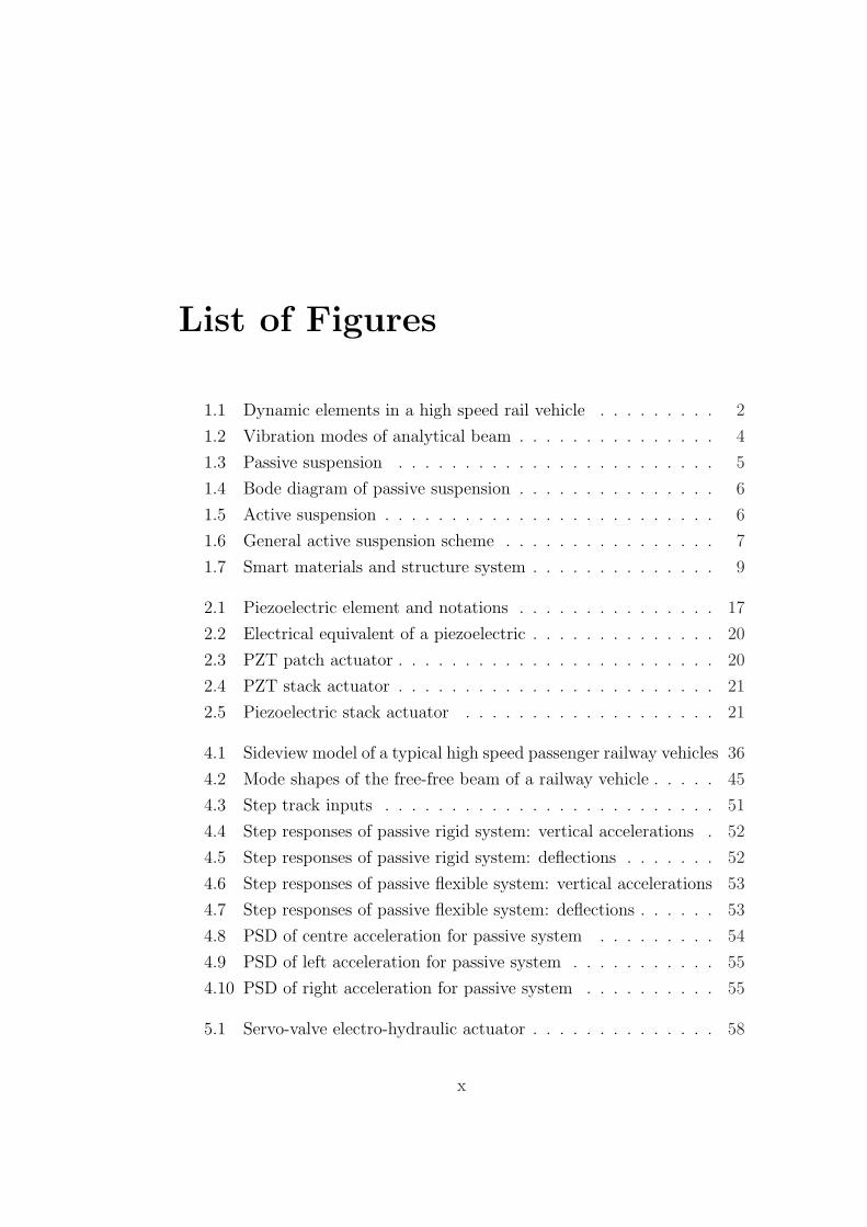
A typical conventional passenger train, as shown by Figure 1.1, consists of
the vehicle body, two bogies and two wheelsets per bogie. Through the
primary suspension, the wheelsets are connected to the bogie, and the bogie
is connected to the vehicle body by secondary suspension. The primary
suspension is so stiff that the bogie will more or less follow the way in
which the track moves vertically as the train travels along. The secondary
suspension is comparatively softer and is aimed to transmit the low frequency
intended movements so the vehicle follows the track, but at the same time to
isolate the higher frequency irregularities. Briefly speaking, the suspension
system provides guidance of the train and helps to maintain the ride comfort
of the passengers.
The vehicle body has 6 degrees of freedom: longitudinal, which is the
1

1.1. RAILWAY TRANSPORTATION
speed of the train, lateral, and vertical, plus three rotational modes: roll,
pitch and yaw. Each bogie has the same degrees of freedom as the vehicle
body. More degrees of freedom come from the springs and dampers. And
extra modes are added if the flexibility of the vehicle body is taken into
account. For vertical suspension control, the side-view model of the railway
vehicle is usually used, which will be described in detail in the Modeling
Chapter (Chapter 4).
Figure 1.1: Dynamic elements in a high speed rail vehicle
In order to keep the competitive position in the whole transportation
industry, there is an impetus for railway vehicles to be increasingly faster.
High speed rail, by definition, is public transport by rail at the speed over
125 km/hour. The first high-speed train in the world, Japan’s Tokaido
Shinkansen built by Kawasaki heavy industries officially launched in 1964,
achieved the speeds of 200km/h. The French TGV set in 1990 reached a
speed of 515 km/h (320 mph), the world speed record for a conventional
2
1.2. PROBLEMS OF HIGH SPEED RAILWAY VEHICLES
wheeled train. The Japanese magnetic levitation (maglev) train has reached
581 km/h (361 mph). High speed train has been proved to be a very efficient
and economical way of transportation.
According to Goodall and Kortum [2002], in a prospective view, future
railway design is aimed to be more cost-effective and energy-efficient. Faster
speed and lighter bodies are the objectives. This becomes feasible both
theoretically and practically with the development of electronics and feedback
control. Actuators, sensors and controller will be at the heart of future
railway vehicles. Furthermore, to take full advantage of control, it is pointed
out that re-design of the mechanical system is needed rather than just adding
electronic control to an existing mechanical system. Thereafter, the system
becomes lighter and mechanically more straightforward by making use of new
lightweight designs and straightforward mechanical configurations.
1.2 Problems of high speed railway vehicles
In order to increase the speed of the railway vehicle and reduce energy
consumption, the vehicle body needs to be designed as light as possible
because heavy bodies limit the operating speed and require actuators of
increased size and power. Due to the light-weight strategy for future high
speed railway vehicle design, the impact of flexibilities of the vehicle body
on ride quality can not be ignored anymore.
The problem with flexible structures lies in the reduced stiffness of
the body, which results in lower natural frequencies. Therefore, increased
flexibility and structural vibrations are easily excited by disturbances from
the outside. This will result in increased levels of high frequency vibrations,
which significantly affect ride quality. Normally vehicle bodies are built
heavier than the bogies so that bogie movements are filtered via the secondary
suspension effectively and do not excite body frequencies. However, as
bodies become lighter, the problem of further excitation of body flexible
frequencies from bogies is evident. Hence the light vehicle bodies regarded
as flexible structures becomes an important issue and suppression of the
vibration of both the rigid modes and flexible modes is required in order
3
1.3. SECONDARY SUSPENSIONS OF RAILWAY VEHICLES
to maintain an acceptable ride comfort or achieve improved ride quality.
Also, the uncertainties associated with flexible structures require the designed
controller to be sufficiently robust.
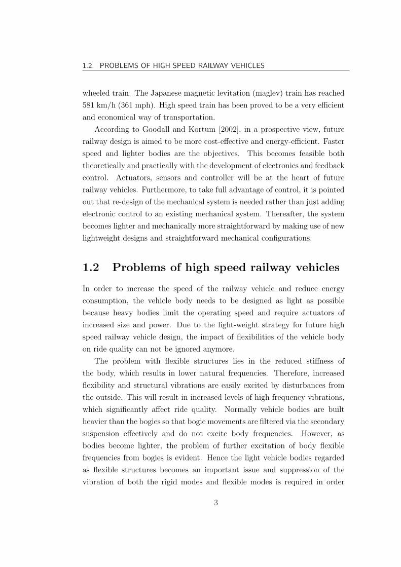
Flexible modes are bending and twisting of the vehicle body due to
external forces acting on it. In this thesis, it is focused on the vertical ride
quality of the vehicle and only the vertical bending modes are considered.
Figure 1.2 shows the vibration modes of the vehicle body when assumed as
a beam. The first vertical bending mode has the largest influence on ride
comfort (Orvnas [2010]).
1st mode(bounce)
2nd mode(pitch)
3rd mode (1st flexible mode)
4th mode(2nd flexible mode)
Figure 1.2: Vibration modes of analytical beam
1.3 Secondary suspensions of railway vehicles
The two main objectives of the secondary suspensions of the railway
vehicle (including primary suspension and secondary suspension as shown
in Figure1.1) are
Achieving good ride quality
Maintaining adequate suspension clearance
The above can be interpreted as minimizing the acceleration of the vehicle
body experienced by passengers without causing large suspension deflections.
The track excitations can be categorized into two types: stochastic, which
4
1.3. SECONDARY SUSPENSIONS OF RAILWAY VEHICLES
is due to track irregularities and deterministic, e.g the gradient or steps of
the track, which is designed by the civil engineers. Ride quality problem is
mainly caused by the track irregularities.
The control design is a multi-objective procedure and there are trade-offs
for the designers to make. In general, the suspension systems in railway
vehicles can be classified into three types:
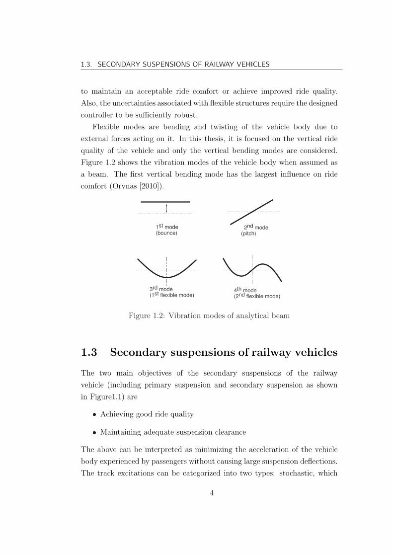
Passive suspensions (e.g Figure 1.3) usually employ springs and pneumatic
or oil dampers. They are simple and cost effective. However, the
performance on the wide frequency range is limited.
Active suspension (e.g Figure 1.5) has high control performance over wide
frequency range while it requires high power and sophisticated control
implementation
Semi-active damping was formally proposed by Karnopp [1974]. It is based
on passive components and its implementations modify the stiffness and
the damping characteristics of the suspension system without the need
to supply a substantial amount of external energy Kallio et al. [2002].
Most commonly used are switched or variable dampers. The control
action of the switched or continuously variable damper attempts to
emulate a fully active control law
mass m
spring
kdamper
c
track input
zt
zm
Figure 1.3: Passive suspension
5

1.3. SECONDARY SUSPENSIONS OF RAILWAY VEHICLES
10−1
100
101
102
−60
−50
−40
−30
−20
−10
0
10
20
Mag
nitu
de (
dB)
Bode Diagram
Frequency (Hz)
GG1
Increased damping
Figure 1.4: Bode diagram of passive suspension
mass m
spring
kdamper
c
track input
zt
zm
Actuator
F
Figure 1.5: Active suspension
With passive suspensions, the performance limits have been reached due
to the inherent trade-offs to be met in the design process, such as increase
in the levels of damping reduces the resonance peak, but it will increase the
transmissibility at higher frequencies as it is shown by Figure 1.4, which is
the Bode diagram of the passive suspension system of Figure 1.3. Also, if the
damping value is too low, it will increase the maximum suspension deflection
during the transient period.
Semi-active control is claimed to be able to offer significant improvements
in performance over passive suspensions whilst avoiding the main drawbacks
6
1.3. SECONDARY SUSPENSIONS OF RAILWAY VEHICLES
associated with the use of active schemes, such as complexity, weight and
cost.
The technology of active suspensions of vehicles has received a great deal
of attention and developments have been made over many decades. In active
suspension, actuators that could provide the function of damping are used in
place of dampers. However, rather than replacing the dampers and springs
by actuators, the actuators are usually added in parallel with an already
optimized passive suspension. Active suspension can ease the inherent trade-
offs. For example, the resonance can be attenuated without increase the
high frequency transmissibility (e.g.skyhook damping). Moreover, active
suspension is especially more effective in suppressing the flexible motions of
a flexible structure, so active suspension make possible the design of lighter-
bodied higher speed railway vehicles. However, it is noted that actuators
are limited in magnitude and bandwidth of forces they can produce. The
bandwidth of the actuator and its ability to avoid having any effect on the
system at higher frequencies is a crucial issue for active suspension control
(Yusof et al. [2011]).
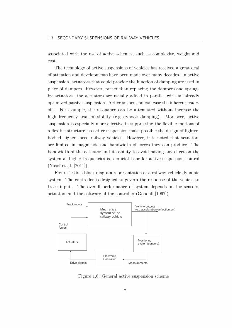
Figure 1.6 is a block diagram representation of a railway vehicle dynamic
system. The controller is designed to govern the response of the vehicle to
track inputs. The overall performance of system depends on the sensors,
actuators and the software of the controller (Goodall [1997])
Mechanicalsystem of therailway vehicle
Vehicle outputs(e.g.acceleration,deflection,ect)
Monitoringsystem(sensors)
ElectronicController
MeasurementsDrive signals
Actuators
Controlforces
Track inputs
Figure 1.6: General active suspension scheme
7
1.4. SMART MATERIALS AND SMART STRUCTURES
1.4 Smart materials and smart structures
Smart materials are materials that have capabilities to respond to environ-
mental stimuli, such as temperature, moisture, PH, or electric and magnetic
fields, to compensate for undesired effects or enhance the desired effects.
Typical examples of smart materials include piezoelectrics, electrostrictives,
magneto-strictives, shape memory alloys (SMA), biomimetic and conductive
polymers, electrochromic coatings, and magneto-rheological (MR), and
electro-rheological (ER) fluids. In general, they possess the capability of
actuating and /or sensing. Smart materials, in scientific literature, are often
called intelligent materials or adaptive materials.
Embedding sensors, actuators, logic and control in structures, such as
bridge, building, composite wings of aircrafts, vehicle bodies, results in
smart structures. In the same way, apart from smart structures, various
terms are also used, such as intelligent structures, adaptive structures, active
structures. Though these terms are quite similar upon their appearances,
they still have great difference in their meanings. Boller [1998] gave his own
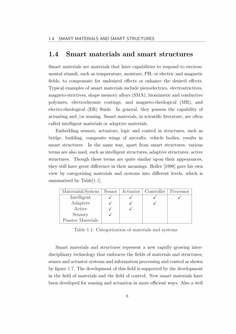
view by categorizing materials and systems into different levels, which is
summarized by Table[1.1].
Materials&System Sensor Actuator Controller ProcessorIntelligent X X X XAdaptive X X XActive X XSensory X
Passive Materials
Table 1.1: Categorization of materials and systems
Smart materials and structures represent a new rapidly growing inter-
disciplinary technology that embraces the fields of materials and structures,
sensor and actuator systems and information processing and control as shown
by figure 1.7. The development of this field is supported by the development
in the field of materials and the field of control. New smart materials have
been developed for sensing and actuation in more efficient ways. Also a well
8

1.5. MOTIVATIONS OF THE RESEARCH
designed and implemented controller plays a significant role in achieving the
smart structure that is desired.
INTELLIGENCE&CONTROL
STRUCTURES Aerospace Civil Transportation...
SENSORSFiber opticPiezoelectric ......
ACTUATORS Piezoelectric SMA ER and MR Fluids ......
Figure 1.7: Smart materials and structure system
The potential application areas of smart materials and structures are
very widespread and include energy conservation, expensive systems with
high potential for operational savings, e.g. transportation systems such as
aircrafts or automobiles, aerospace structures, civil infrastructure, structural
health monitoring, intelligent highways, high-speed railways, active noise
suppression, robotics(Jr et al. [1996]). A number of smart materials can
be used for vibration control purposes as actuators and sensors such as
piezoelectric, shape memory, electrostrictive and magnetostrictive materials.
Piezoelectric actuators and sensors have been extensively used in vibration
control applications and will be considered in this thesis.
1.5 Motivations of the Research
Smart structures are considered to have the capability to contribute to vibra-
tion suppression of flexible structures, hence improving system performance.
With integrated sensors and actuator materials, they might eliminate the
need for extensive heavy mechanical actuation systems. Therefore, the
system will be lighter in weight, consume less energy and achieve higher
performance levels through their functionality for suppressing vibrations.
Much research has been done for improving the ride quality of flexible-
bodied railway vehicles: 1) by improvements in suspension control design
9
1.6. RESEARCH AIMS AND OBJECTIVES
or 2) by structural damping through the concept of smart structure aiming
at reducing the vehicle body structural vibration. In this research, it is
motivated to use both of the two approaches, complementary to each other,
to improve the ride quality of the railway vehicles. Therefore, the idea of
suppressing the vibration of flexible-bodied railway vehicle through smart
structure and active secondary suspensions is proposed. Smart actuators
are to be incorporated into flexible structures, i.e. flexible bodied railway
vehicles, combining with appropriate control strategies, to realize vibration
suppression and robust control to improve the performance of the system.
Clearly the need of studying in-depth the flexible railway structure
incorporated smart materials from both a theoretical and practical point
of view is of great importance. It is to take a rigorous study of the flexible
railway structure with smart materials, to investigate the feasibility of the
smart material for railway application, and to incorporate control solutions
based on selected sensor/actuator configuration.
1.6 Research aims and objectives
The aim of the proposed research is to contribute towards the improvement
of the performance of a flexible bodied high-speed railway vehicle via the use
of smart materials in addition to active secondary suspension control, thus
minimizing vibrations to achieve satisfactory control of both the rigid body
modes and flexible modes with certain robustness.
The objectives of this research are
1. Investigate the feasibility of introducing piezoelectric actuators and
sensors to the flexible railway structure for effective ride quality
enhancement at high-speeds.
2. Rigorous modeling of the flexible-bodied railway vehicle.
3. Placement of actuators and sensors to achieve the required performance
with minimum effort of control.
10

1.6. RESEARCH AIMS AND OBJECTIVES
4. Development of appropriate control strategies. Comparison between
the application of different control laws (e.g. centralized/desentrolized
control, classical control method, optimal control method, robust
control method etc.)
1.6.1 Thesis structure
The thesis is organized as follows:
Chapter 2 is a detailed survey of work involving active suspension
control of railway vehicles and suppressing of flexible modes of the
vehicle body with piezoelectric actuators and sensors.
Chapter 3 introduces the track profile and the assessment methods used
in this thesis, which includes power spectral density analysis, root mean
square value assessment by covariance analysis and by time domain
analysis.
Chapter 4 provides a detailed modeling of the side-view model of a
typical flexible-bodied railway vehicle with stack piezoelectric actuators
mounted on the vehicle body.
Chapter 5 covers a brief study of the dynamic of the electro-servo
hydraulic actuator used for the secondary suspension control, the
design of a inner loop PID controller for the hydraulic actuator, brief
introduction of the piezoelectric actuators and sensors used in this
thesis, and finally the placement of actuators and sensors.
Chapter 6 is a preliminary control study on active suspension control
in order to demonstrate the necessity of controlling of the flexibility
of the vehicle body to achieve better ride quality. Classical method of
modal control with skyhook damping and advanced control method of
LQG control are applied and the results are compared. The effect of
dynamics of the electro-servo hydraulic actuator on the performance of
the system is finally evaluated.
11
1.7. SUMMARY
Chapter 7 describes the design of the decentralized controller. Active
suspension controller aimed to reduce the rigid modes and the controller
for active structural damping aimed to reduce the flexible modes of
the vehicle body are the two sub controllers. Two control methods,
modal controller with skyhook damping and LQG control are applied
for control design.
Chapter 8 describes the design of the centralized controller. Modern
control approaches H2 control, H∞ control are applied and a new tech-
nology, model predictive control technology based on mixed H2/H∞control approach are applied.
Chapter 9 contains a conclusion on the work that is done in this thesis
and suggestion for future work.
1.7 Summary
This chapter briefly introduced the railway transportation and the tendency
of development for future fast speed flexible-bodied railway vehicles. The
research problem is defined, the new concept for solving the problem is
proposed, the aim of the research is identified. Finally, the objectives for
achieving the aim are presented.
12

Chapter 2
Literature Review
In this chapter, a literature review is provided on relevant work to this
research. The first section covers work related to active suspension of railway
vehicles, which also covers the suppressing of the flexible motion with active
suspension control. The second section is a coverage on work of application
of smart materials/structures for vibration control purposes, especially with
piezoelectric actuators. The third part is a survey on research on improving
the ride quality of flexible-bodied railway vehicles with piezoelectric actuators
and sensors. Finally a review is done on the methods for actuator and sensor
placement.
2.1 Vibration control of railway vehicles
2.1.1 Active suspension control
Good ride quality of railway vehicles is usually achieved by a careful design of
the secondary suspension system. With passive suspensions, the performance
limits have been reached due to the inherent trade-offs to be met in the design
process (Pratt [1996]). Active suspension provides improved performance in
relaxing the many conflicting requirements for suspension system of a railway
vehicle. Karnopp [1978] discussed the need for active suspensions. Orvnas
[2008] provides a comprehensive literature survey of concepts and previous
work on active secondary suspension in trains.
13

2.1. VIBRATION CONTROL OF RAILWAY VEHICLES
Control methods that are usually used can be categorized into classical
control and modern model-based strategies (e.g. optimal control, H-infinity
control).
Classical control scheme is simple and believed much easier to apply than
advanced control methods (Williams [1986]). Skyhook damping is usually
used as the introduction to active suspension control. Besides, it is also a
good start point for developing the controller (Foo and Goodall [2000]). It
controls the resonance of the suspension without making things worse at
high frequencies. However, skyhook damping can create large suspension
deflections when gradients and curves are encountered.
Modern control methods are capable of achieving a more complicated
multi-objective control and balance well between different or even conflicting
performance requirements, but they usually result in very complex controllers
and may be difficult to implement (Goodall and Kortum [2002]). For
example, the optimal control theory finds its regulator in minimizing a pre-
scribed performance function that may involve various kinds of criteria. The
advantages are that it ensures a stable closed-loop system with guaranteed
levels of stability robustness (Foo and Goodall [2000]). This control method
is good in theory but more difficult to implement. Nevertheless, it has been
used by many researchers (Pratt [1996], Paddison [1995] and Foo and Goodall
[2000]).
Li and Goodall [1999] compared different control strategies for applying
skyhook damping control in active suspension systems for railway vehicles.
Williams [1986] compared classical and optimal control methods for active
suspension systems. Pratt [1996] conducted a comprehensive study of the
active suspension applied to railway trains. Modified skyhook damping
method, complementary filter control and optimal control were used for the
secondary vertical active suspension control. Foo and Goodall [2000] applied
classical control methods using skyhook damping and optimal control method
for active suspension control of flexible-bodied railway vehicles. H∞ control
approach was applied by Tsunashima and Morichika [2004] for ride quality
improvement of an AGT vehicle. Ray [1992] studied active suspension control
of an one quarter car using the LQG-LTR approach and it proved to be robust
14

2.1. VIBRATION CONTROL OF RAILWAY VEHICLES
by stochastic robustness analysis.
2.1.2 Vibration suppression of the flexible modes
As recent railway vehicles are manufactured increasingly lighter to achieve
high speed, suppression of the motion of flexible modes of vehicle bodies has
become essential in improving the ride comfort of railway vehicles. According
to Takigami and Tomioka [2008] and Schirrer and Kozek [2008], methods
that have already been proposed can be categorized into two complementary
approaches: (1) applying active/semi-active suspension control (2) structural
damping (passive or active). In this section, the literature survey is focused
on the first approach. In the next section, the applications of piezoelectric
technology for structural damping will be given.
The problem of suppressing the flexible modes started to be addressed
very early for ground vehicles. Nagai and Sawada [1987] designed the active
suspension system not only to control the rigid body motions but also
to suppress the bending vibrations of a high speed ground vehicle. The
characteristics of the actuator (the pneumatic suspension) was taken into
consideration. The motion of vehicle body was divided into odd-function
mode and even-function mode by modal decomposition. Decentralized
optimal modal control that assumes the vertical motions of the body at
front and rear are independent was applied. Then centralized optimal modal
control was also employed, where odd-function mode and the even-function
mode were controlled independently.
Capitani and Tibaldi [1989] studied the active suspension of a flexible
vehicle. Firstly, a full LQG regulator was designed based on the full
model that includes both the rigid body modes and flexible body modes.
Then a reduced controller was designed by only taking account of the rigid
body model. The performance of the full controller and reduced controller
were compared. It was claimed that whether the reduced controller give
satisfactory performance is dependent on the trade-off between the regulation
cost and the control energy.
Hac [1986, 1989] studied active suspension control of a half car model
15
2.2. SMART MATERIALS AND STRUCTURES
including elastic modes. Optimal control theory was adopted. The
performance index included various criteria such as ride comfort, road
tracking ability, hardware limitations.
Hac et al. [1996a,b] evaluated the effectiveness of active suspensions and
subsequently semi-active suspensions in reducing the structural vibrations of
a vehicle body. Their work emphasized on making the controller itself more
aware of the flexible modes. Skyhook damping control was found effective
for rigid body vehicles, but it did not perform as satisfactorily in reducing
structural resonances as a passive system.
Wu et al. [2004] used semi-active suspension for vibration control of the
high-speed vehicle. Elastic deformation effect was considered in a multi-body
system dynamical model of the car body structure. It was shown that the
ride indices on the car body floor in the place of bogie centre between the
flexible car body model and rigid car body model had not much difference,
but there was a big difference in the place of car body centre.
Foo and Goodall [2000] placed a third actuator in addition to two
secondary suspension actuators at the centre of the vehicle for reducing the
effects of first flexible mode of the vehicle body. Both classical control method
with skyhook damping and Optimal control method were applied.
Sugahara et al. [2007] proposed a method by controlling the damping
force of axle dampers installed between bogie frames and wheel sets. Semi-
active controller was applied to determine the optimal damping force based
on the skyhook control theory.
2.2 Smart materials and structures
Chopra [2002] gives an comprehensive review of state of the art of smart
structures and integrated systems. Boller [1998] provides the state of the art
and trends in using smart materials and systems in transportation vehicles.
Hurlebaus and Gaul [2005] gives an overview of research in several fields
of application of smart structure dynamics technologies. Active vibration
control through the use of piezoelectric materials is included.
16

2.2. SMART MATERIALS AND STRUCTURES
2.2.1 Piezoelectric materials
The piezoelectric effect was discovered by Pierre and Jacques Curie in 1880 ,
but it was not fully used until 1940s (Ahmadian and DeGuilio [2001]). Now
piezoelectric materials have been widely used as sensory and active materials
in many applications in the field of smart structures for flexible structure
vibration control due to their accuracy in sensing and actuation, light weight,
and ability to generate large force without reaction.
Piezoelectric materials can transfer mechanical energy to electrical energy
or conversely, electrical energy to mechanical energy. When a piezoelectric
material is mechanically stressed it develops an electrical charge across its
terminals. This effect is known as the piezoelectric effect. Conversely, an
electric field or charge that is applied to the same material will produce
mechanical strain. This effect is referred to the converse piezoelectric effect.
Therefore, piezoelectricity is the combined effect of the electrical behavior
of the material and Hooke’s Law. Consider a typical piezoelectric transducer
as in Figure 2.1. The strain-charge form of the constitutive equations of the
v
3(z)
1(x)
2(y)
p
Electrode
Electrode
DiopleAlighnment
Appliedfield E
Figure 2.1: Piezoelectric element and notations
piezoelectric transducer are
Si = sEijTj + dmiEm (2.1)
Dm = dmiTi + ξTikEk (2.2)
17
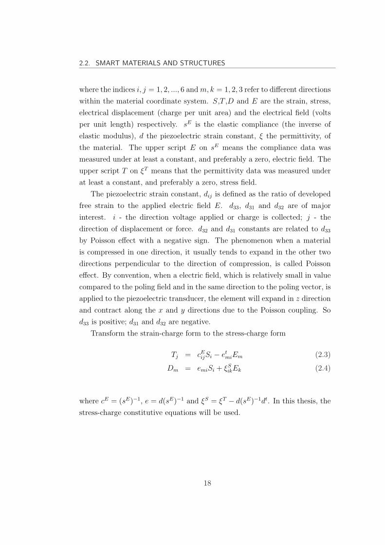
2.2. SMART MATERIALS AND STRUCTURES
where the indices i, j = 1, 2, ..., 6 and m, k = 1, 2, 3 refer to different directions
within the material coordinate system. S,T ,D and E are the strain, stress,
electrical displacement (charge per unit area) and the electrical field (volts
per unit length) respectively. sE is the elastic compliance (the inverse of
elastic modulus), d the piezoelectric strain constant, ξ the permittivity, of
the material. The upper script E on sE means the compliance data was
measured under at least a constant, and preferably a zero, electric field. The
upper script T on ξT means that the permittivity data was measured under
at least a constant, and preferably a zero, stress field.
The piezoelectric strain constant, dij is defined as the ratio of developed
free strain to the applied electric field E. d33, d31 and d32 are of major
interest. i - the direction voltage applied or charge is collected; j - the
direction of displacement or force. d32 and d31 constants are related to d33
by Poisson effect with a negative sign. The phenomenon when a material
is compressed in one direction, it usually tends to expand in the other two
directions perpendicular to the direction of compression, is called Poisson
effect. By convention, when a electric field, which is relatively small in value
compared to the poling field and in the same direction to the poling vector, is
applied to the piezoelectric transducer, the element will expand in z direction
and contract along the x and y directions due to the Poisson coupling. So
d33 is positive; d31 and d32 are negative.
Transform the strain-charge form to the stress-charge form
Tj = cEijSi − et
miEm (2.3)
Dm = emiSi + ξSikEk (2.4)
where cE = (sE)−1, e = d(sE)−1 and ξS = ξT − d(sE)−1dt. In this thesis, the
stress-charge constitutive equations will be used.
18
2.2. SMART MATERIALS AND STRUCTURES
2.2.2 Control with piezoelectric actuators and sensors
Piezoelectric actuators and sensors have been extensively used in vibration
control applications. Ahmadian and DeGuilio [2001] gives a good review
on the recent developments on piezoceramics for vibration suppression. The
review of previous research proves that PZT with different control schemes
can be used to significantly reduce structural noise and vibration without
adding any significant amount of weight to the structure. Most of the studies
of PZT, both experimental and analytical, for noise and vibration suppression
are still on relatively simple structures such as beams and plates. Halim
and Moheimani [2001] conducted a comprehensive research on vibration
analysis and control of smart structures. The research was concentrated on
flexible structures and using piezoelectric materials as actuators and sensors.
It covered the topic of modeling smart structures, optimal placement of
actuators and sensors and spatial H2/H∞ control of flexible structures.
Two commonly used piezoelectric materials are polyvinylidene fluoride
(PVDF), a semicrystalline polymer film, and lead zirconate titanate(PZT),
a piezoelectric ceramic material. PVDF is much more compliant and
lightweight, thus more attractive for sensing applications. PZT is more
favoured as an actuator since PZT has larger electromechanical coupling
coefficients than PVDF so PZT can induce larger forces or moments on
structures. It is shown that PZT can be effectively used as a transducer
for vibration control of flexible structures(Halim [2002]).
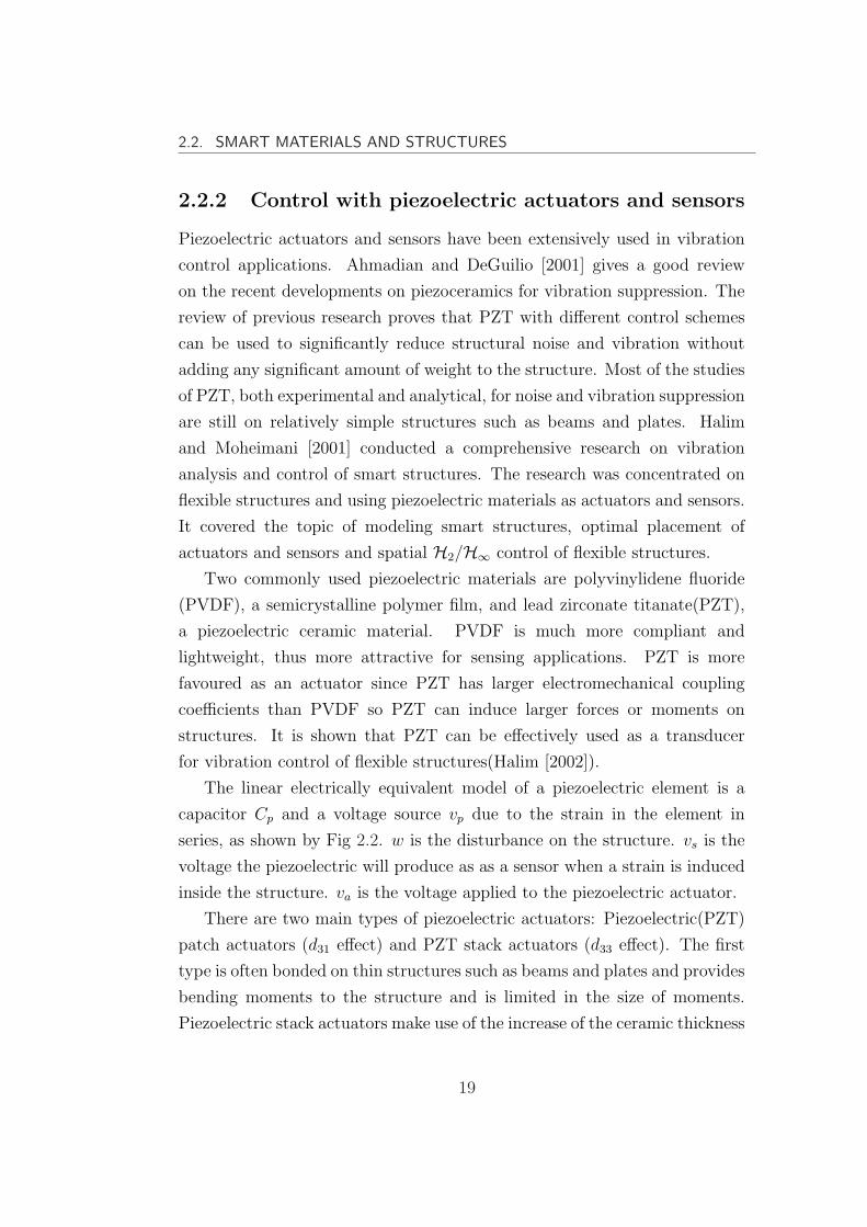
The linear electrically equivalent model of a piezoelectric element is a
capacitor Cp and a voltage source vp due to the strain in the element in
series, as shown by Fig 2.2. w is the disturbance on the structure. vs is the
voltage the piezoelectric will produce as as a sensor when a strain is induced
inside the structure. va is the voltage applied to the piezoelectric actuator.
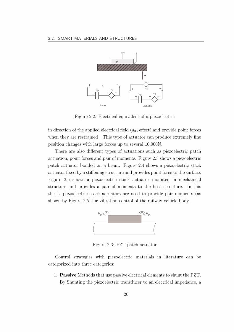
There are two main types of piezoelectric actuators: Piezoelectric(PZT)
patch actuators (d31 effect) and PZT stack actuators (d33 effect). The first
type is often bonded on thin structures such as beams and plates and provides
bending moments to the structure and is limited in the size of moments.
Piezoelectric stack actuators make use of the increase of the ceramic thickness
19
2.2. SMART MATERIALS AND STRUCTURES
xxxxxxxxxxxxxxxxxxxxxxxxxxxxxxxxxxxxxxxxxxxxxxxxxxxxxxxxxxxxxxxxxxxxxxxxxxxxxxxxxxxxxxxxxxxxxxxxxxxxxxxxxxxxxxxxxxxxxxxxxxxxxxxxxxxxxxxxxxxxxxxxxxxxxxxxxxxxxxxxxxxxxxxxxxxxxxxxxxxxxxxxxxxxxxxxxxxxxx
P
w
xxxxx
xxxxxxxxxxxxx
Cp vp
vs
Cp vp
va
Sensor Actuator
Figure 2.2: Electrical equivalent of a piezoelectric
in direction of the applied electrical field (d33 effect) and provide point forces
when they are restrained . This type of actuator can produce extremely fine
position changes with large forces up to several 10,000N.
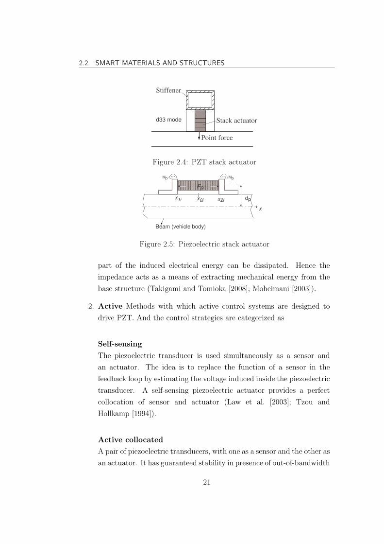
There are also different types of actuations such as piezoelectric patch
actuation, point forces and pair of moments. Figure 2.3 shows a piezoelectric
patch actuator bonded on a beam. Figure 2.4 shows a piezoelectric stack
actuator fixed by a stiffening structure and provides point force to the surface.
Figure 2.5 shows a piezoelectric stack actuator mounted in mechanical
structure and provides a pair of moments to the host structure. In this
thesis, piezoelectric stack actuators are used to provide pair moments (as
shown by Figure 2.5) for vibration control of the railway vehicle body.
MpMp
Figure 2.3: PZT patch actuator
Control strategies with piezoelectric materials in literature can be
categorized into three categories:
1. Passive Methods that use passive electrical elements to shunt the PZT.
By Shunting the piezoelectric transducer to an electrical impedance, a
20
2.2. SMART MATERIALS AND STRUCTURES
xxxxxxxxxxx
xxxxxxxxxxxx
xx
xx
x
xxxxxxxxxxxxxxxxxxxxxxxx
xxxx
xxxx
xx
Stiffener
Point force
Stack actuatord33 mode
Figure 2.4: PZT stack actuator
xxxxxxxxxxxxxxxxxxxxxxxxxxxxxxxxxxxxxxxxxxxxxxxxxxxxxxxxxxxxxxxxxxxxxxxxxxxxxxxxxxxxxxxxxxxxxxxxxxxxxxxxxxxxxxxxxxxxxxxxxxxxxxxxxxxxxxxxxxxxxxxxxxxxxxxxxxxxxxxxxxxxxxxxxxxxxxxxxxxxxx
xxxxx xxxxxFp
xxxxxxxxxxxxxxxxxxxxxxxxxxxxxxxxxxxxxxxxxxxxxxxxxxxxxxxxxxxxxxxxxxxxx x
x1i x2ixxxxxxxxxxx
dp
MpMp
x0i
xxxxxxxxxxxxxx
xxxxxxxxx
xxxx
xxxxxxx
xxxxxxxxxxxx
Beam (vehicle body)
xxxxxxxxxxxxxx
xxxxxxxxx
xxx x
xxxxxxx
xxxxxxxxxxxx
Figure 2.5: Piezoelectric stack actuator
part of the induced electrical energy can be dissipated. Hence the
impedance acts as a means of extracting mechanical energy from the
base structure (Takigami and Tomioka [2008]; Moheimani [2003]).
2. Active Methods with which active control systems are designed to
drive PZT. And the control strategies are categorized as
Self-sensing
The piezoelectric transducer is used simultaneously as a sensor and
an actuator. The idea is to replace the function of a sensor in the
feedback loop by estimating the voltage induced inside the piezoelectric
transducer. A self-sensing piezoelectric actuator provides a perfect
collocation of sensor and actuator (Law et al. [2003]; Tzou and
Hollkamp [1994]).
Active collocated
A pair of piezoelectric transducers, with one as a sensor and the other as
an actuator. It has guaranteed stability in presence of out-of-bandwidth
21

2.2. SMART MATERIALS AND STRUCTURES
dynamics (Halim and Moheimani [2002]; Moheimani [2005]).
Active non-collocated
Measured signals are used to determine the electric power through a
designed controller and feedback to the piezo actuator (Kamada et al.
[2005]). A stronger vibration reduction can be achieved with a non-
collocated scheme (Benatzky and Kozek [2008])
3. Hybrid and semiactive Methods that combine the shunted and
active control techniques (Law et al. [2003]; Tzou and Hollkamp [1994]).
2.2.3 Piezoelectric technology for flexible-bodied vehi-
cles
There has been much research on applying piezoelectric for vibration control
of flexible-bodied railway vehicles. Both passive (Takigami and Tomioka
[2008]; Hansson et al. [2003]) and active (Kamada et al. [2005]; Schandl et al.
[2007]) control schemes have been tried. In some of the studies, the model
of the railway vehicle is simplified to a flexible beam (Kamada et al. [2005,
2008]), and experiments have been done on scaled vehicle bodies (Takigami
and Tomioka [2008]; Kozek et al. [2009]; Benatzky et al. [2007]). However
the feasibility of a full-scale implementation is still not very clear.
With passive method, piezoelectric elements are shunted by electric
circuits to reduce the bending vibration of railway vehicles. Vibration
energy is converted to electrical energy, which is then dissipated in a shunt
circuit (Takigami and Tomioka [2008, 2005]; Hansson et al. [2003]). Kamada
et al. [2008] introduced two strategies for shunt damping using piezoelectric
stack transducers for vibration suppression of railway vehicle to enhance ride
quality and good robustness against mass perturbation was confirmed.
An active damping concept was applied to the suppress the structural
vibration modes of a car body with piezoelectric actuators by Kamada et al.
[2005]. Independent H∞ controllers were designed for the first three flexible
modes with only one acceleration sensor and five piezoelectric actuators. The
22

2.2. SMART MATERIALS AND STRUCTURES
effectiveness of the controller was verified on a 1/6 scaled model experiment
setup with piezoelectric actuators embedded to the setup.
In the research by Schandl et al. [2007], piezo-stack actuators were
also proposed and studied in improving the ride comfort of light weight
railway vehicles. The piezo-stack actuators mounted in consols together
with collocated sensor patches were attached to the structure. A centralized
control scheme was applied. The output signals of the sensors for measuring
the flexible deformation of the car body were used in a feedback control loop,
and a bending moment was generated and directly applied to the car body
by the actuators. State feedback controller was designed with the method of
pole placement and the states were estimated from the sensor signals.
Kozek et al. [2009] extended the work of Schandl et al. [2007]. Col-
located strain sensors and piezoelectric actuators were used to introduce
force/moments pairs into the car body structure for improving passenger
ride comfort. Robust H∞ control was applied and the design steps are
illustrated, nonlinear actuator dynamics were modeled and compensated,
optimal placement of actuators and sensors was addressed and the feasibility
of the proposed concept was demonstrated in laboratory experiments.
Benatzky et al. [2007] compared controller design utilizing the µ-synthesis
procedure and pole-placement combined with Kalman-filter techniques and
their implementation on a 1/10 scaled flexible structure experiment of a
metro vehicle car body. A better performance was achieved by µ-synthesis
procedure because of the fact that the uncertainty associated with the
model of the structure as well as the fact of the performance variables to
be controlled are not identical to the measurements. At the same time
considerably lower control cost was needed with µ-synthesis controller.
Based on the studies carried by Benatzky et al. [2007], Schirrer and Kozek
[2008] proposed the use of co-simulation for effective and efficient verification
and validation of the control design for metro rail vehicle car bodies because
controller design is usually carried out on order-reduced or simplified models.
23
2.2. SMART MATERIALS AND STRUCTURES
2.2.4 Modeling and analysis of smart structures
Modeling of smart structures is not solely about modeling of flexible struc-
tures, but also about modeling of the smart actuators and sensors attached
to the structure. For basic studies, a good description of general methods of
modeling of continuous structures is provided by Bishop and Johnson [1960].
When the complicated shapes and structural patterns make the development
and solution of descriptive partial differential equations burdensome, they
are considered modeled as either lumped or distributed parameter systems.
Various discretization techniques, such as finite element(FE) modeling,
modal analysis and lumped parameters have been widely used in literature
(Foo and Goodall [2000], Tohtake et al. [2005], Kozek et al. [2009]), which
allow the approximation of the partial differential equations.
The system model can be formulated analytically or by system identifica-
tion. According to Kozek et al. [2009], a suitable model for controller design
can be derived from its FE model in the design stage, which is essential
for control concept studies and actuator and sensor placement optimization.
However, due to limited model accuracy, it is advised to use a more accurate
model from an identification procedure for final controller computation and
implementation.
The technique of modal analysis allows the vibratory motion to be
represented by an infinite series of mode shapes, multiplied by system time
dependent coordinates, which govern the participation of each mode shape
in the overall motion. The number of modes is necessarily reduced to a finite
number in order to achieve a workable mathematical model, while in the
other hand the truncation of the number of modes leads to a limitation in the
accuracy of the model. Instability can be caused by the unmodeled dynamics.
With control design that has sufficient robust properties can overcome the
bad effects that may be caused by the truncated models (Gavin [Jan 2001]).
Popprath et al. [July 2006] investigated an approximately 1/10-scaled
model of a metro vehicle car body concerning the low structural eigenmodes.
In the research by Schandl et al. [2007] and Schirrer and Kozek [2008], a
multibody model of the flexible-bodied railway vehicle was developed by
24
2.3. ACTUATOR AND SENSOR PLACEMENT
modal approach to represent the flexible deformations and finite-element
method is employed for calculating the set of eigenfunctions. Frequency
response modes (FRMs) was used for modeling essential local deformations
caused by the moment input of the actuators which can not be represented
sufficiently by modal approach. Mechatronic damping system was applied
by Kamada et al. [2005] and Schandl et al. [2007] for generating the stiffness
and structural damping, which are not necessarily provided by the structure
itself in the design of extremely light-weight railway vehicles.
2.3 Actuator and sensor placement
The placement of actuators and sensors on a flexible structure for vibration
control plays an important role in achieving a good performance.
Criteria for the optimal placement of actuators and sensors are given
in Gawronski [1999], Gawronski [2004] and Leleu et al. [2001]. Gawronski
[2004] introduced criteria for optimal actuator/sensor placement based on the
H2, H∞ or the Hankel system norm of the transfer function matrices from
the actuators to the sensors. In general the positions with strongest local
deformations are to be selected. The placement criterion by Leleu et al. [2001]
is based on state controllability/observability. The controllability gramian
Wc /observability gramian Wo and the standard deviation of the eigenvalues
σ(λi) are used, thus the criterion accounts for model uncertainties.
Hac and Liu [1993] gave a systematic method for solving the problem of
optimal sensor and actuator placement in the control of flexible structures.
The optimization criteria are chosen based on the energies of the input
and the output when the flexible structures is imposed with transient and
persistent disturbances.
Aldraihem [1997] formulated an optimization criterion for size and
location of piezoelectric actuators/sensors patches bonded a beam. The
criterion is based on the degree of modal controllablility and practical
considerations. The modes are weighed differently according to their
importance to the system.
Benatzky and Kozek [2008] investigated the influence of the actuator size
25

2.4. SUMMARY
on the closed-loop stability of collocated and non-collocated transfer function
models utilized in the structural control of flexible beams.
2.4 Summary
This literature review has covered the work on active suspension control
of railway vehicles for improving the ride quality, vibration control with
piezoelectric actuators and sensors and the application of the piezoelectric
actuators and sensors for improving the ride quality of flexible-bodied railway
vehicles. Aspects of modeling of flexible structures, control methods/strate-
gies, and placement of actuators and sensors have been included.
26
Chapter 3
Assessment Methods
A reliable accurate assessment of the performance is of importance in the
development of active suspension controllers of a railway vehicle. Ride quality
and suspension deflections are the two important aspects in evaluating
suspension performance.
Ride quality is generally characterized by the root mean square (RMS)
accelerations of the vehicle body in response to disturbances from the track.
The appearance of ride quality differs depending on the choice of weights,
statistical approaches or evaluation formulae.
Throughout this thesis, the RMS accelerations of the vehicle body in
gravity%, the suspension deflections in millimeteres, the suspension control
inputs in Newtons, the control inputs from piezoelectric actuators in Volts
and the power spectral density (PSD) of the accelerations and the control
inputs are used as measures of the performance of the system. Three methods
for analysis, namely frequency response analysis, covariance analysis and
time history analysis for measuring ride quality are used. In this chapter,
the track inputs subjected to the railway vehicle and these three methods for
measuring ride quality are to be introduced.
27
3.1. TRACK PROFILE
3.1 Track profile
Railway vehicles are dynamically-complex systems which are subject to a
variety inputs from the track, which can be categorized into two categories:
1. Stochastic(random) inputs due to track irregularities, i.e. random
changes in the track vertical, lateral, and cross level positions.
2. Deterministic inputs, such as steps, curves and gradients.
The study in this thesis is concerned with the vertical ride quality of a railway
vehicle running on a straight track. Track irregularities are the primary cause
of ride degradation. Therefore, only the stochastic inputs, i.e. the vertical
random track irregularities, are considered.
3.1.1 Track irregularities
The irregularities of a railway track can be represented by a spatial power
spectrum, which is normally approximated as a fourth order equation (Pratt
[1996])
SS(fs) =Ωv
f 2s + 5.86f 3
s + 17.29f 4s
m2(cycle/m)−1 (3.1)
where Ωv is the vertical track roughness in m and fs is the spatial frequency
of the track in cycle/m.
It is widely accepted to approximate Equation (3.1) by a simpler
expression by neglecting the higher terms.
SS(fs) =Ωv
f 2s
m2(cycle/m)−1 (3.2)
In order to be used in dynamic analysis, the information given in Equation
(3.2) needs to be converted into temporal form.
The dynamic modes of a railway vehicle lie between 0.1Hz and 20Hz,
it will therefore be excited by track inputs in this frequency range. The
relationship between the spatial wavelengths and the temporal excitation is
velocity dependent
fs(cycles/m) =ft(cycles/s)
v(m/s)(3.3)
28

3.1. TRACK PROFILE
Substituting (3.3) into (3.2), the track wavelengths in terms of the temporal
frequency ft is given by
SS(ft) =Ωvv
2
f 2t
m2(cycle/m)−1 (3.4)
Expression (3.4) can be converted to a spectrum with a temporal base when
divided by the speed v(m/s)
ST (ft) =SS(ft) m2(cycle/m)−1
v (m/s)(3.5)
The wheelsets are connected directly to dampers and this necessitates
track velocities as an input if the model of the railway vehicle is to be
expressed in a state-space form. Therefore, it is needed to convert the vertical
track displacement spectrum given by (3.5) into its derivative. Firstly,
convert (3.5) so that ST (ft) is expressed in terms of radians rather than
cycles
ST (ft) =Ωvv
2πf 2t
m2(rad/s)−1 (3.6)
The derivative of the spectrum is derived by multiplying the spectrum by
(2πft)2
ST (ft) (m/s)2(rad/s)−1 = ST (ft) m2(rad/s)−1 × (2πft)2 (3.7)
which gives
ST (ωt) = 2πΩvv (ms−1)2(rad/s)−1 (3.8)
Finally convert the expression back to the representation in terms of cycles
rather than radians
ST (ft) = (2π)2Ωvv (ms−1)2(Hz)−1 (3.9)
The vertical track spectrum is flat over all frequencies, and it is in essence
white noise with a Gaussian distribution. The approximations made earlier
ignoring the fourth order expression in favor of the simpler inverse-square
29
3.2. FREQUENCY DOMAIN ANALYSIS
relationship give rise to the infinite bandwidth of this white noise, otherwise
a high frequency roll-off of the expression given by (3.1) would occur giving
rise to a finite bandwidth velocity spectrum. In this research, the random
track is generated from (3.9) and a track roughness 2.5×10⁻⁷ m is used (Foo
[2000]), which typically corresponds to a good quality track.
3.2 Frequency domain analysis
The frequency domain technique can be used to evaluate vehicle ride quality
and suspension deflections in response to track irregularities and the PSD
plots of the signals of interest.
The output power spectrum Sy(ω) is equal to the square of the modulus of
the system transfer function H(jω) multiplied by the input power spectrum
Sω(ω)
Sy(ω) = H(jω)H(−jω)Sω(ω) = |H(jω)|2Sω(ω) (3.10)
To account for the time delay, tdelay, between the front and rear wheelset.
H(jω) needs to be modified to
H(jω) = Hf (jω) + Hr(jω)e−jωtdelay (3.11)
where Hf (jω) is the transfer function from the front velocity input to the
output, and Hr(jω) is the transfer function from the rear velocity input to
the output.
The RMS values of the signal can be obtained from
σ(ω) =
√∫ ∞
0
|H(jω)|2Sω(ω) (3.12)
Equation (3.12) requires numerical integration to infinity, which is not
practically possible. Hence a finite limit is used instead. This does not pose
a problem for railway vehicle application as the higher frequency components
are usually attenuated by the suspension dynamics and the effect is negligible.
30
3.3. COVARIANCE ANALYSIS
3.3 Covariance analysis
A summary on covariance analysis will be provided in this section (Foo
[2000] and Paddison [1995]). Covariance analysis is based on Lyapunov
equation. The system model can be represented by the following state-space
formulation
x = Ax + Bww (3.13)
y = Cx + Dww (3.14)
where A is the state matrix, Bw the disturbance input matrix and w the
disturbance input.
The RMS values of the outputs are calculated from the solution of
Lyapunov equation. It requires all the elements of the feedforward matrix
Dw to be zero, i.e. the model is strictly proper. In addition, white noise
input is required.
The autocorrelation function of the track input is derived from the track
PSD function
Ew(t)wT (t + τ) =
∫ ∞
−∞ST (
ω
2π)eωτjdω (3.15)
After performing the integration, the autocorrelation may be stated more
simply as
Ew(t)wT (t + τ) = (2π)2Ωvvδ(τ) = qwδ(t− τ) (3.16)
The variance is simply the value of the autocorrelation function at zero,
qw(0). The track disturbance input is a Gaussian white noise process. This
can be used in Lyapunov equation to provide the stationary state covariance
matrix Px (Px = 0) of the system given by (3.14)
APx + PxAT + BwqwBT
w = 0 (3.17)
Px is a positive definite square matrix, and is symmetric if BwqwBTw is
symmetric. It should be noted that the positive definite solution of the
31
3.3. COVARIANCE ANALYSIS
Lyapunov equation exists only for stable systems and Px is finite only when
the system is strictly proper. Then the covariance of the output vector is
given by
σ2 = CPxCT (3.18)
The RMS value is given by
σ =√|σ2| (3.19)
However, the system concerned in this thesis is driven by two random
velocity inputs from the track, which are Gaussian white noise processes.
For the railway vehicle of length Lv and a traveling speed of v m/s, there
will be a time delay between the front and rear input due to the distance
between the front and rear bogies. The front and rear velocity are related by
ZR(t) = ZL(t− tdelay) (3.20)
With a constant track variance given by (3.9), the auto-correlation function
of the track input in this instance is
Qw = (2π)2Ωvv
[δ(t− τ) δ(t− τ + tdelay)
δ(t− τ − tdelay) δ(t− τ)
](3.21)
Then
BwQwBw = (2π)2Ωvv[BwLBTwL+BwRBT
wR+BwRBTwLeAT tdelay+eAtdelayBwLBT
wR]
(3.22)
In equation 3.22, Qw is the covariance, which is the auto-correlation function
at zero. Instead of solving (3.17), solving the following equation for Px
APx + PxAT + BwQwBT
w = 0 (3.23)
Finally the variance of the system can be calculated by (3.18)
32

3.4. TIME DOMAIN ANALYSIS
3.4 Time domain analysis
In time domain, it is to find the RMS (root mean square) of a signal by
investigating the vehicle model output responses with respect to the track
data recordings. The RMS value for a given output can be found using
yrms =√
E[y2(t)] =
√lim
T→∞
∫ T
0
y2dt (3.24)
or approximately
yrms ≈√√√√ 1
n
n∑i=1
y2i (3.25)
where n is the number of elements in the data sample. It is easily seen that
the accuracy of the RMS value depends upon the available duration of track
data T , and the number of sample points n (in other words, it depends upon
the available number of sample points and the sampling interval). Therefore,
a sufficiently long track together with an adequate number of sample points
should be selected in order to achieve accurate RMS results
To analyze the frequency information of the signal, fast Fourier transform
(FFT) can be performed to the output response of the railway vehicle model
by simulating it with the track data. Similarly, a sufficiently long duration
of track data and an adequate number of points should be used to reveal
accurate information of the signal frequency content.
Though the time history analysis methods are slower and less accurate
than covariance and frequency methods. Time analysis is the best solution
when the model contains non-linearities or it is difficult to get a linear model
of the system because both the covariance and frequency methods can only
be used with a linear model.
3.5 Summary
This chapter has described the representation of the track irregularities.
Vertical ride quality of a railway vehicle running on a straight track is of
33

3.5. SUMMARY
main concern of this thesis. Track irregularities are the primary cause of ride
degradation. It has introduced the method of frequency response analysis for
calculating the PSDs of signals of interest, and method of covariance analysis
and time history analysis for calculating r.m.s values.
34
Chapter 4
Derivation of the Model
4.1 Overview
It is very important to obtain a sufficiently accurate model of the system
for control design. In this chapter, the side-view model of a flexible-bodied
railway vehicle is derived. Flexibility in the bodies of high-speed railway
vehicles creates a number of difficulties which in practice may result in the
body structure being heavier than it might otherwise be. When an active
suspension is used it becomes particularly important to model the vehicle
and its flexibility in an effective manner because: (i) active control might
inadvertently excite the flexible modes (ii) there is also the opportunity to
control the flexibility.
The vehicle body of the railway vehicles is to be assumed as a flexible
free-free beam, which is justified because the secondary suspension is very
soft that the vehicle body moves in the manner of a free-free beam. Both
the flexible modes and rigid modes will be included in the model. The bogie
will be considered rigid and are connected with the vehicle body with various
suspension elements (i.e. spring and dampers). The system is subject to three
inputs sources: track disturbances, the control forces provided across the
secondary suspensions and the control moments provided by the piezoelectric
actuators attached to the railway vehicle body.
35
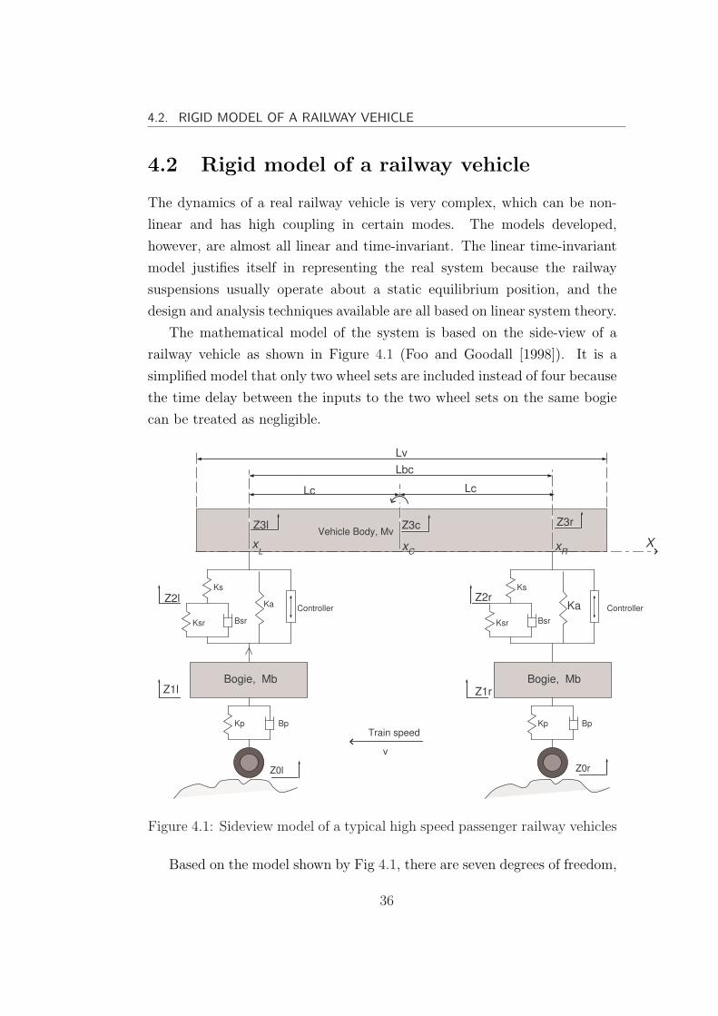
4.2. RIGID MODEL OF A RAILWAY VEHICLE
4.2 Rigid model of a railway vehicle
The dynamics of a real railway vehicle is very complex, which can be non-
linear and has high coupling in certain modes. The models developed,
however, are almost all linear and time-invariant. The linear time-invariant
model justifies itself in representing the real system because the railway
suspensions usually operate about a static equilibrium position, and the
design and analysis techniques available are all based on linear system theory.
The mathematical model of the system is based on the side-view of a
railway vehicle as shown in Figure 4.1 (Foo and Goodall [1998]). It is a
simplified model that only two wheel sets are included instead of four because
the time delay between the inputs to the two wheel sets on the same bogie
can be treated as negligible.
Ks
Ksr Bsr
KaController
Bogie, Mb
Kp Bp
Ks
Ksr Bsr
Ka Controller
Bogie, Mb
Kp Bp
Vehicle Body, Mv
Lv
Lbc
Lc Lc
Z3l
Z0rZ0l
Z3c Z3r
Z2l
Z1l
Z2r
Z1r
Train speed
v
xL
xC
xR
X
Figure 4.1: Sideview model of a typical high speed passenger railway vehicles
Based on the model shown by Fig 4.1, there are seven degrees of freedom,
36
4.2. RIGID MODEL OF A RAILWAY VEHICLE
i.e. the vehicle body’s bounce mode and pitch mode, the bounce modes of
the two bogie masses, and two modes associated with the internal dynamics
of the air spring. When flexibility is considered, extra flexible modes of the
vehicle body will be added. However, in this section, it is to first derive rigid
model of the railway vehicle.
The vehicle body is influenced by the forces generated by the passive
secondary suspension components: Ks, Ka, Ksr, Bsr, and by the active
control forces from the actuators across the secondary suspensions on the
left and the right : UL, UR. The bogie motions are effected by both and
primary suspension components, i.e. Kp and Bp, and the passive secondary
components as well as the reaction of the active secondary forces. The
primary suspension is subjected to the disturbances from the track Z0L and
Z0R.
For a system with more than a few degrees of freedom, it becomes a
cumbersome way to derive the equations of motion with Newton’s second law
of motion. Lagrangian Equation will be used to establish the equations of
motions of the railway vehicles. Lagrange’s equation provides a systematic
unified approach for handling the modeling problems of a wide range of
physical systems. The differential equations that describe the system will be
readily obtained once the systematic procedure is carried out. It is especially
advantageous to use Lagrange’s equation to model large complex systems, for
it deals with the model from the energy point of view. Lagrange’s Equation
is given byd
dt(∂T
∂pn
)− ∂T
∂pn
+∂D
∂pn
+∂V
∂pn
= Qn (4.1)
where n = 1, 2, ... denotes the number of independent coordinates that exist
in the system; pn is the generalized coordinate; pn is the generalized velocity;
T is the total kinetic energy of the system; D is the dissipation function of the
system; V is the total potential energy of the system; Qn is the generalized
applied force at the coordinate n.
For the convenience of modeling, we assume that there are two small
masses, mL → 0 and mR → 0, locating at where displacements of Z2L and
Z2R are measured respectively. The energy expressions for the system given
37
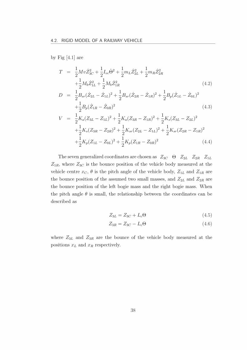
4.2. RIGID MODEL OF A RAILWAY VEHICLE
by Fig [4.1] are
T =1
2MvZ2
3C +1
2IvcΘ
2 +1
2mLZ2
2L +1
2mRZ2
2R
+1
2MbZ
21L +
1
2MbZ
21R (4.2)
D =1
2Bsr(Z2L − Z1L)2 +
1
2Bsr(Z2R − Z1R)2 +
1
2Bp(Z1L − Z0L)2
+1
2Bp(Z1R − Z0R)2 (4.3)
V =1
2Ka(Z3L − Z1L)2 +
1
2Ka(Z3R − Z1R)2 +
1
2Ks(Z3L − Z2L)2
+1
2Ks(Z3R − Z2R)2 +
1
2Ksr(Z2L − Z1L)2 +
1
2Ksr(Z2R − Z1R)2
+1
2Kp(Z1L − Z0L)2 +
1
2Kp(Z1R − Z0R)2 (4.4)
The seven generalized coordinates are chosen as Z3C Θ Z2L Z2R Z1L
Z1R, where Z3C is the bounce position of the vehicle body measured at the
vehicle centre xC , θ is the pitch angle of the vehicle body, Z1L and Z1R are
the bounce position of the assumed two small masses, and Z2L and Z2R are
the bounce position of the left bogie mass and the right bogie mass. When
the pitch angle θ is small, the relationship between the coordinates can be
described as
Z3L = Z3C + LcΘ (4.5)
Z3R = Z3C − LcΘ (4.6)
where Z3L and Z3R are the bounce of the vehicle body measured at the
positions xL and xR respectively.
38

4.2. RIGID MODEL OF A RAILWAY VEHICLE
Apply the Lagrange’s equation of equation (4.1) to the system
d
dt(
∂T
∂Z3C
)− ∂T
∂Z3C+
∂D
∂Z3C
+∂V
∂Z3C= Ur + Uc + Uf (4.7)
d
dt(∂T
∂Θ)− ∂T
∂Θ+
∂D
∂Θ+
∂V
∂Θ= UrLc − UfLc (4.8)
d
dt(
∂T
∂Z2L
)− ∂T
∂Z2L+
∂D
∂Z2L
+∂V
∂Z2L= 0 (4.9)
d
dt(
∂T
∂Z2R
)− ∂T
∂Z2R+
∂D
∂Z2R
+∂V
∂Z2R= 0 (4.10)
d
dt(
∂T
∂Z1L
)− ∂T
∂Z1L+
∂D
∂Z1L
+∂V
∂Z1L= −Uf (4.11)
d
dt(
∂T
∂Z1R
)− ∂T
∂Z1R+
∂D
∂Z1R
+∂V
∂Z1R= −Ur (4.12)
The differential equations obtained from equation (4.9), (4.10) are
Bsr(Z2L − Z1L) + Ks(Z2L − Z3C + Lcθ)−Ksr(Z1L − Z2L) = 0 (4.13)
Bsr(Z2R − Z1R) + Ks(Z2R − Z3C + Lcθ)−Ksr(Z1R − Z2R) = 0 (4.14)
It should be noted that the states Z2R and Z2L can be eliminated from the
rest of the differential equations by substituting in their expressions in terms
of other states, which are solved out from equations (4.13) and (4.14).
Lagrangian equations use degrees of freedom of the structure to describe
the dynamic of the system. If represented in state-space form, the dynamic
of the system is described by system states. The number of system states
are usually equal or larger than twice the number of degrees of freedom of
freedom. The state-space representation of the model is formed as
xr = Arx + Bru + Gw (4.15)
where matrices Ar, Br, and G the system matrix, force input matrix ,
disturbance input matrix, and xr the states of the system are set as
xr = [ Z3C Z3C Z1L Z1L Z1R Z1R Z2L Z2R Θ Θ] (4.16)
39
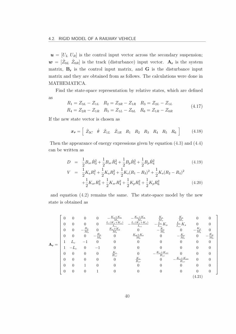
4.2. RIGID MODEL OF A RAILWAY VEHICLE
u = [UL UR] is the control input vector across the secondary suspension;
w = [Z0L Z0R] is the track (disturbance) input vector. Ar is the system
matrix, Br is the control input matrix, and G is the disturbance input
matrix and they are obtained from as follows. The calculations were done in
MATHEMATICA.
Find the state-space representation by relative states, which are defined
asR1 = Z3L − Z1L R2 = Z3R − Z1R R3 = Z2L − Z1L
R4 = Z2R − Z1R R5 = Z1L − Z0L R6 = Z1R − Z0R
(4.17)
If the new state vector is chosen as
xr =[
Z3C θ Z1L Z1R R1 R2 R3 R4 R5 R6
](4.18)
Then the appearance of energy expressions given by equation (4.3) and (4.4)
can be written as
D =12BsrR
23 +
12BsrR
24 +
12BpR
25 +
12BpR
24 (4.19)
V =12KaR
21 +
12KaR
22 +
12Ks(R1 −R3)2 +
12Ks(R2 −R4)2
+12KsrR
23 +
12KsrR
24 +
12KpR
25 +
12KpR
26 (4.20)
and equation (4.2) remains the same. The state-space model by the new
state is obtained as
Ar =
0 0 0 0 −Ks+Ka
Mv−Ks+Ka
Mv
Ks
Mv
Ks
Mv0 0
0 0 0 0 Lc(Ks+Ka)Ivc
−Lc(Ks+Ka)Ivc
− Lc
IvcKs
Lc
IvcKs 0 0
0 0 −Bp
Mb0 Ka+Ks
Mb0 −Ks
Mb0 −Kp
Mb0
0 0 0 −Bp
Mb0 Ka+Ks
Mb0 −Ks
Mb0 −Kp
Mb
1 Lc −1 0 0 0 0 0 0 01 −Lc 0 −1 0 0 0 0 0 00 0 0 0 Ks
Bsr0 −Ks+Ksr
Bsr0 0 0
0 0 0 0 0 Ks
Bsr0 −Ks+Ksr
Bsr0 0
0 0 1 0 0 0 0 0 0 00 0 0 1 0 0 0 0 0 0
(4.21)
40
4.3. MODEL OF THE FLEXIBLE STRUCTURE
Br =
1Mv
1Mv
− Lc
Ivc
Lc
Ivc
− 1Mb
00 − 1
Mb
0 00 00 00 00 00 0
(4.22)
G =
0 00 0
Bp
Mb0
0 Bp
Mb
0 00 00 00 0−1 00 −1
(4.23)
4.3 Model of the flexible structure
The flexible body of the railway vehicle is assumed as a free-free Euler-
Bernoulli beam of length, l, cross section area, Ab, material density, ρb and
flexural rigidity, EI, which depends on the Young’s modulus of elasticity
E and the second moment of area I. The flexural vibration of the beam
is induced by the excitations transmitted through the suspensions from the
track disturbances. Here it is assumed that there are np stack piezoelectric
actuators attached to the surface of the beam to suppress the flexure
vibration of the beam.
These are the main assumptions about the flexible structure
Bernoulli-Euler theory is used as the method of analysis, it assumes
that plane cross-sections of the beam remain plane during flexure and
the radius of curvature of a bent beam is large compared with the
beam’s depth (Bishop and Johnson [1960]).
41
4.3. MODEL OF THE FLEXIBLE STRUCTURE
The mass and stiffness contributions of the piezoelectric elements are
considerably smaller than those of the beam so they can be ignored.
The transverse deflection at point x of the beam and time t is denoted
by v(x, t), assuming the beam is one-dimension only. The governing PDE
(Partial differential equation) that describes the dynamics of the structure
of the flexible beam is given as follows (Halim et al(2002)).
EI∂4v(x, t)
∂x4+ρbAb
∂2v(x, t)
∂t2=
np∑i=1
∂2Mpx(x, t)
∂x2+FxL
(t)δ(x−l1)+FxR(t)δ(x−l2)
(4.24)
where FxLand FxR
are the forces from the left and right suspensions.
i=1,2..., np denote the number of piezoelectric actuators, Mpx the moment
acting on the beam by the piezoelectric actuators, which is given by (Halim
et al(2001))
M ipx(x, t) = KaVai[H(x− x1i)−H(x− x2i)] (4.25)
where Vai is the voltage applied to the ith actuator. H(.) is the step function.
x1i and x2i denote the location of the two ends of the ith piezoelectric actuator
along the X axis. And Ka is a constant based on the properties of the beam
and the piezoelectric actuators. The first forcing term in PDE equation (4.24)
can be determined from equation (4.25), using the property of Dirac’s delta
function
∫ ∞
−∞δ(n)(t− θ)φ(t)dt = (−1)nφ(n)(θ) (4.26)
where δ(n) is the nth derivative of δ and φ is continuous at θ.
The beam equation contains a fourth-order derivation in x, so four
boundary conditions are needed to find a unique solution z(x, t). Since no
external bending moment and no external force are applied at the free ends
of the beam, the bending moment and the shear force at the free ends are
42

4.3. MODEL OF THE FLEXIBLE STRUCTURE
zero. Therefore, the end conditions for both free ends of the beam are
∂2z(x, t)
∂x2|x=0=
∂3z(x, t)
∂x3|x=0= 0 (4.27)
∂2z(x, t)
∂x2|x=Lv=
∂3z(x, t)
∂x3|x=Lv= 0 (4.28)
where the x coordinate of the left end and the right end of the beam are 0
and Lv respectively.
By the modal analysis technique, the solution of the transverse deflection
v(x, t) is assumed to be in the form
v(x, t) = z3c(t) + θ(t)(x− Lb/2) +∞∑
r=1
qr(t)φr(x) (4.29)
where qr(t) is the rth flexible mode in generalized coordinate and φr(x) is
the corresponding mode shape(eigenfunction), which is determined from the
eigenvalue problem
φr(x) = cosh λrx + cos λrx− cosh(λrl)− cos(λrl)
sinh(λrl)− sin(λrl)
(sinh(λrx) + sin(λrx)) (4.30)
The frequency equation of an undamped free-free beam is
cos(λrl) cosh(λrl)− 1 = 0 (4.31)
Through equation (4.31), a series of λr can be determined, and the
corresponding natural frequencies ωr determined by
λ4 =ω2Abρb
EI(4.32)
43
4.3. MODEL OF THE FLEXIBLE STRUCTURE
The eigenfunction mode shapes have orthogonality properties
∫ L
0
φr(x)φp(x)dx = δrp (4.33)
∫ L
0
EI
ρbAb
d4φr(x)
dx4φp(x)dx = ω2
rδrp (4.34)
where δrp is the Kronecker delta function.
The flexible motions can be denoted by a set of uncoupled ordinary
differential equations, which can be obtained by integrating equation (4.24)
over the beam length, using the orthogonality properties of equation
(4.33)and (4.34) and Dirac’s delta function property of equation (4.26) as
well as the solution in 4.29.
qr(t) + 2ζrωrqr(t) + ω2rqr(t) =
Ka
∑np
i=1 ΨriVai(t) + FxLφr(l1) + FxR
φr(l2)
Mb(4.35)
where ωr is the natural frequency of the rth flexible mode. Structural damping
is added and ζr is the damping ratio of the rth flexible mode. Mb is the mass
of the beam, and Ψri is given by
Ψri =dφr
dx(x2i)− dφr
dx(x1i) (4.36)
Ψri is for the ith piezoelectric actuator, and is a function of the position
of the piezoelectric actuator, x0i, and the length of the actuator Lp.
The multi-input-infinite-output transfer function from the applied actu-
ator voltages Va(s) to the beam deflection Z(x, s) at location x, is written
as
G(x, s) =Ka
Mb
∞∑r=1
φr(x)ΨTr
s2 + 2ζrωr + ω2r
(4.37)
where
Va(s) = [Va1(s), ..., Vanp(s)]T (4.38)
ΨTr = [Ψr1Ψr2 · · ·Ψrnp ] (4.39)
44
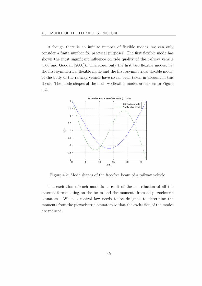
4.3. MODEL OF THE FLEXIBLE STRUCTURE
Although there is an infinite number of flexible modes, we can only
consider a finite number for practical purposes. The first flexible mode has
shown the most significant influence on ride quality of the railway vehicle
(Foo and Goodall [2000]). Therefore, only the first two flexible modes, i.e.
the first symmetrical flexible mode and the first asymmetrical flexible mode,
of the body of the railway vehicle have so far been taken in account in this
thesis. The mode shapes of the first two flexible modes are shown in Figure
4.2.
0 5 10 15 20 25−2
−1.5
−1
−0.5
0
0.5
1
1.5
2Mode shape of a free−free beam (L=27m)
x(m)
φ(x)
1st flexible mode2nd flexible mode
Figure 4.2: Mode shapes of the free-free beam of a railway vehicle
The excitation of each mode is a result of the contribution of all the
external forces acting on the beam and the moments from all piezoelectric
actuators. While a control law needs to be designed to determine the
moments from the piezoelectric actuators so that the excitation of the modes
are reduced.
45
4.4. FLEXIBLE MODEL OF THE RAILWAY VEHICLE
4.4 Flexible model of the railway vehicle
According to the ODE equation (4.35), the ordinary differential equations of
the first two flexible motions can be written as
q1(t) + 2ζ1ω1q1(t) + ω21q1(t) =
FxLφ1(xL) + FxR
φ1(xR)
Mv
+Ka
Mv
np∑i=1
Ψ1iVai(t)
(4.40)
q2(t) + 2ζ2ω2q2(t) + ω22q2(t) =
FxLφ2(xL) + FxR
φ2(xR)
Mv
+Ka
Mv
np∑i=1
Ψ2iVai(t)
(4.41)
where F3L and F3R are given by
FxL= FKs(xL) + FKa(xL) + UL (4.42)
FxR= FKs(xR) + FKa(xR) + UR (4.43)
where FKs and FKa are forces generated by springs Ks and Ka
FKs(xL) = −Ks(ZxL− Z2L) (4.44)
FKa(xL) = −Ka(ZxL− Z1L) (4.45)
FKs(xR) = −Ks(ZxR− Z2R) (4.46)
FKa(xR) = −Ka(ZxR− Z1R) (4.47)
where ZxLand ZxR
are the vertical displacement of vehicle body at position
xL and xR
ZxL= Z3L + q1(t)φ1(xL) + q2(t)φ2(xL) (4.48)
ZxR= Z3R + q1(t)φ1(xR) + q2(t)φ2(xR) (4.49)
Substituting equations (4.42)and (4.43) into equations (4.40) and (4.41),
and by using equations (4.44)- (4.47), (4.48) and (4.49), it is found the matrix
46

4.4. FLEXIBLE MODEL OF THE RAILWAY VEHICLE
representation of equation (4.40)-(4.41) in terms of all the states of the system
˙xflex = Arfxrigid + Afxflex + Bf1u + Bf2Va (4.50)
where
x = [ xrigid xflex ] (4.51)
where
xrigid =[
Z3C θ Z1L Z1R R1 R2 R3 R4 R5 R6
]
xflex = [ q1 q1 q2 q2 ]
u = [Ul UR]
Va = [Va1(s)...Vanp(s)] (4.52)
and
Arf =
0 0 0 0 − (Ks+Ka)φ1(xL)Mv
− (Ka+Ks)φ1(xR)Mv
Ksφs(xL)Mv
Ksφs(xR)Mv
0 0
0 0 0 0 0 0 0 0 0 0
0 0 0 0 − (Ka+Ks)φ2(xL)Mv
− (Ka+Ks)φ2(xR)Mv
Ksφa(xL)Mv
Ksφa(xR)Mv
0 0
0 0 0 0 0 0 0 0 0 0
(4.53)
Af =
−2ζ1ω1 −ω21 − 2(Ka+Ks)φ2
1(xL)
Mv0 0
1 0 0 0
0 0 −2ζ2ω2 −ω22 − 2(Ka+Ks)φ2
2(xL)
Mv
0 0 1 0
(4.54)
47
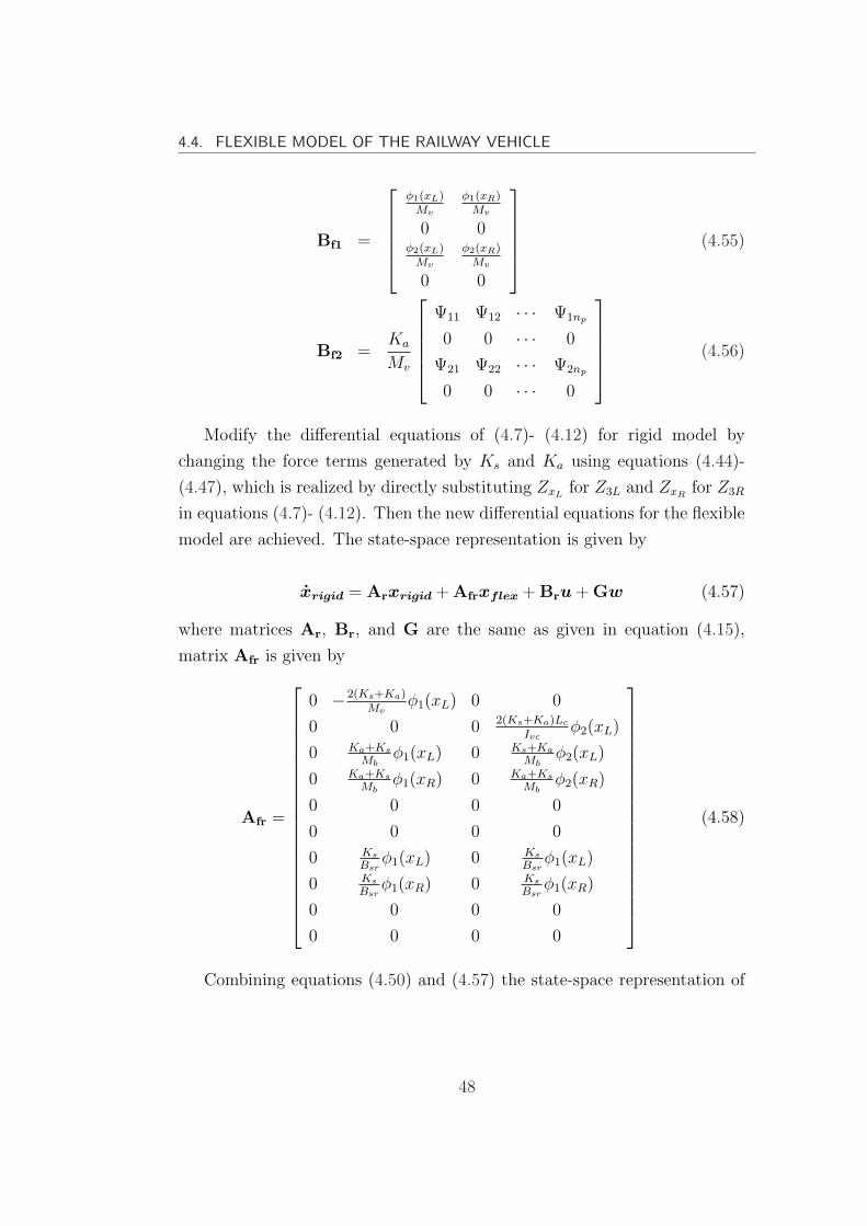
4.4. FLEXIBLE MODEL OF THE RAILWAY VEHICLE
Bf1 =
φ1(xL)Mv
φ1(xR)Mv
0 0φ2(xL)
Mv
φ2(xR)Mv
0 0
(4.55)
Bf2 =Ka
Mv
Ψ11 Ψ12 · · · Ψ1np
0 0 · · · 0
Ψ21 Ψ22 · · · Ψ2np
0 0 · · · 0
(4.56)
Modify the differential equations of (4.7)- (4.12) for rigid model by
changing the force terms generated by Ks and Ka using equations (4.44)-
(4.47), which is realized by directly substituting ZxLfor Z3L and ZxR
for Z3R
in equations (4.7)- (4.12). Then the new differential equations for the flexible
model are achieved. The state-space representation is given by
xrigid = Arxrigid + Afrxflex + Bru + Gw (4.57)
where matrices Ar, Br, and G are the same as given in equation (4.15),
matrix Afr is given by
Afr =
0 −2(Ks+Ka)Mv
φ1(xL) 0 0
0 0 0 2(Ks+Ka)Lc
Ivcφ2(xL)
0 Ka+Ks
Mbφ1(xL) 0 Ks+Ka
Mbφ2(xL)
0 Ka+Ks
Mbφ1(xR) 0 Ka+Ks
Mbφ2(xR)
0 0 0 0
0 0 0 0
0 Ks
Bsrφ1(xL) 0 Ks
Bsrφ1(xL)
0 Ks
Bsrφ1(xR) 0 Ks
Bsrφ1(xR)
0 0 0 0
0 0 0 0
(4.58)
Combining equations (4.50) and (4.57) the state-space representation of
48
4.5. COUPLING BETWEEN RIGID MOTION AND FLEXIBLE MOTION
the model of a flexible-railway vehicle is given by
x =
[Ar(12× 12) Afr(12× 4)
Arf (4× 12) Af (4× 4)
]x +
[Br
Bf1
]u +
[0
Bf2
]V a +
[G
0
]w
(4.59)
where Afr and Arf are called (flexible-rigid) and (rigid-flexible) coupling
matrices respectively.
4.5 Coupling between rigid motion and flex-
ible motion
According to the explanation by Gevarter [1970], the coupling between the
rigid motion and the flexible motion, as we imagine, is introduced by control
and takes places in two ways, i.e. actuation and sensing. In the way of
actuation, the forces and moments that are applied to control the rigid body
motion will also excite the flexible motions, qr. The rigid body control, e.g.
Fc, is converted to the generalized force, Fn, by a factor, i.e. φr(h)
Fn = φr(h)Fc (4.60)
In the way of sensing, the sensors that were designed to sense the rigid body
motion for feedback control purpose will also sense the flexible motion, e.g.
qr. The factor(mode shape), i.e. φr(x), is used to convert the rth generalized
coordinate, qr, into the quantity, vr, sensed by the sensors.
vr = qrφr(x) (4.61)
Besides active control using real actuators and sensors, the passive control
elements springs Ks and Ka can be also viewed as collocated sensor and
actuators. The vertical displacement that are sensed by springs (Ks and Ka)
in the secondary suspension consists of the rigid modes as well as the flexible
modes, which in turn changed the forces that are produced by the springs
when they are functioning as actuators.
49
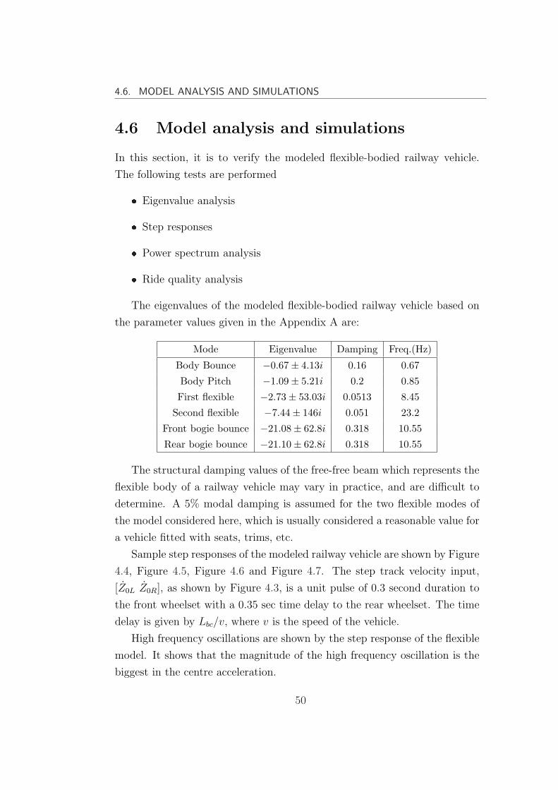
4.6. MODEL ANALYSIS AND SIMULATIONS
4.6 Model analysis and simulations
In this section, it is to verify the modeled flexible-bodied railway vehicle.
The following tests are performed
Eigenvalue analysis
Step responses
Power spectrum analysis
Ride quality analysis
The eigenvalues of the modeled flexible-bodied railway vehicle based on
the parameter values given in the Appendix A are:
Mode Eigenvalue Damping Freq.(Hz)
Body Bounce −0.67± 4.13i 0.16 0.67
Body Pitch −1.09± 5.21i 0.2 0.85
First flexible −2.73± 53.03i 0.0513 8.45
Second flexible −7.44± 146i 0.051 23.2
Front bogie bounce −21.08± 62.8i 0.318 10.55
Rear bogie bounce −21.10± 62.8i 0.318 10.55
The structural damping values of the free-free beam which represents the
flexible body of a railway vehicle may vary in practice, and are difficult to
determine. A 5% modal damping is assumed for the two flexible modes of
the model considered here, which is usually considered a reasonable value for
a vehicle fitted with seats, trims, etc.
Sample step responses of the modeled railway vehicle are shown by Figure
4.4, Figure 4.5, Figure 4.6 and Figure 4.7. The step track velocity input,
[Z0L Z0R], as shown by Figure 4.3, is a unit pulse of 0.3 second duration to
the front wheelset with a 0.35 sec time delay to the rear wheelset. The time
delay is given by Lbc/v, where v is the speed of the vehicle.
High frequency oscillations are shown by the step response of the flexible
model. It shows that the magnitude of the high frequency oscillation is the
biggest in the centre acceleration.
50
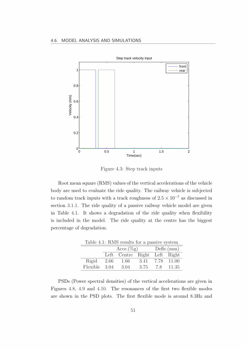
4.6. MODEL ANALYSIS AND SIMULATIONS
0 0.5 1 1.5 20
0.2
0.4
0.6
0.8
1
Time(sec)
Vel
ocity
(m
/s)
Step track velocity input
frontrear
Figure 4.3: Step track inputs
Root mean square (RMS) values of the vertical accelerations of the vehicle
body are used to evaluate the ride quality. The railway vehicle is subjected
to random track inputs with a track roughness of 2.5× 10⁻⁷ as discussed in
section 3.1.1. The ride quality of a passive railway vehicle model are given
in Table 4.1. It shows a degradation of the ride quality when flexibility
is included in the model. The ride quality at the centre has the biggest
percentage of degradation.
Table 4.1: RMS results for a passive system
Acce.(%g) Defle.(mm)Left Centre Right Left Right
Rigid 2.66 1.66 3.41 7.78 11.00Flexible 3.04 3.04 3.75 7.8 11.35
PSDs (Power spectral densities) of the vertical accelerations are given in
Figures 4.8, 4.9 and 4.10. The resonances of the first two flexible modes
are shown in the PSD plots. The first flexible mode is around 8.3Hz and
51
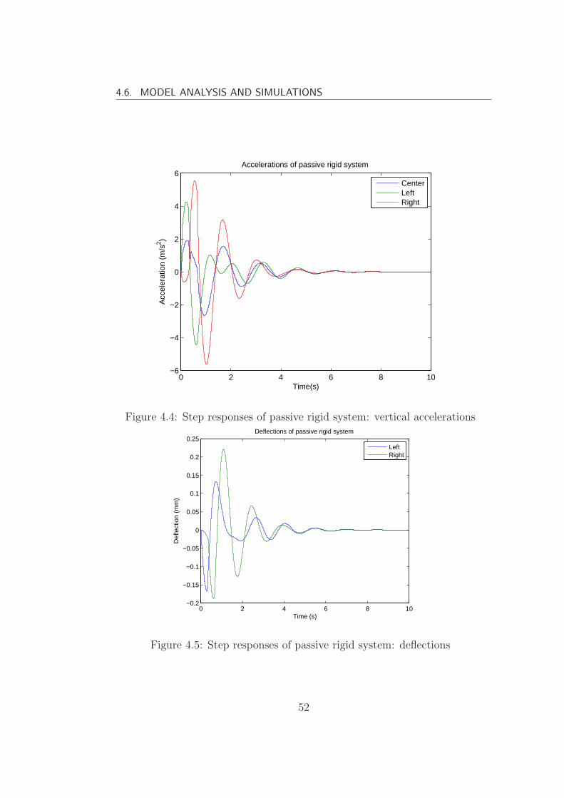
4.6. MODEL ANALYSIS AND SIMULATIONS
0 2 4 6 8 10−6
−4
−2
0
2
4
6Accelerations of passive rigid system
Time(s)
Acc
eler
atio
n (m
/s2 )
CenterLeftRight
Figure 4.4: Step responses of passive rigid system: vertical accelerations
0 2 4 6 8 10−0.2
−0.15
−0.1
−0.05
0
0.05
0.1
0.15
0.2
0.25Deflections of passive rigid system
Time (s)
Def
lect
ion
(mm
)
LeftRight
Figure 4.5: Step responses of passive rigid system: deflections
52
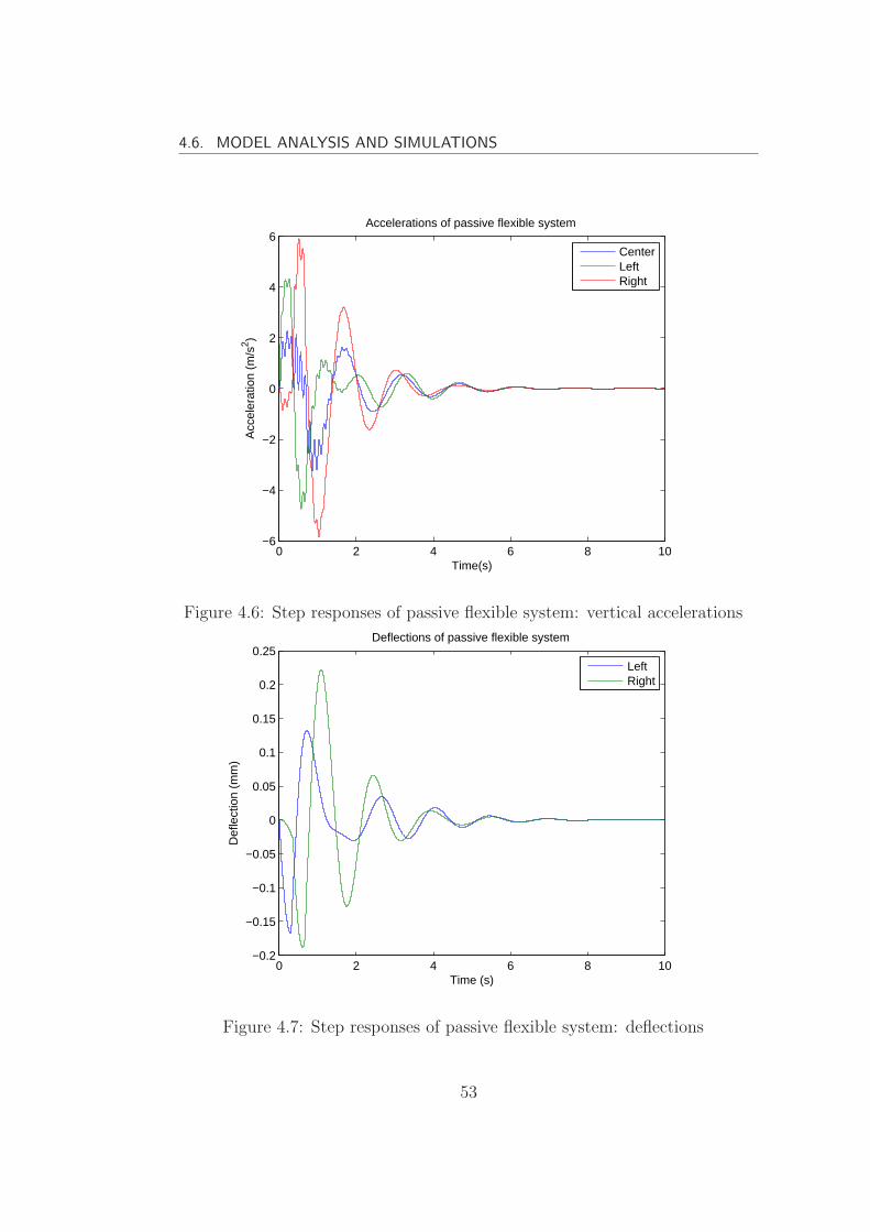
4.6. MODEL ANALYSIS AND SIMULATIONS
0 2 4 6 8 10−6
−4
−2
0
2
4
6Accelerations of passive flexible system
Time(s)
Acc
eler
atio
n (m
/s2 )
CenterLeftRight
Figure 4.6: Step responses of passive flexible system: vertical accelerations
0 2 4 6 8 10−0.2
−0.15
−0.1
−0.05
0
0.05
0.1
0.15
0.2
0.25Deflections of passive flexible system
Time (s)
Def
lect
ion
(mm
)
LeftRight
Figure 4.7: Step responses of passive flexible system: deflections
53

4.7. SUMMARY
is the main cause of vertical bending. The second mode which is around
23Hz has become very small. This shows that it is reasonable to just include
the first two flexible modes in the model for control design. The dips shown
in centre acceleration PSD in Figure 4.8 are caused by geometric filtering.
However, it is not an effect in the left and right accelerations because they
are combinations of bounce and pitch modes.
0 5 10 15 20 25 3010
−40
10−30
10−20
10−10
100
PSD of Center Acceleration
Frequency(Hz)
(m/s
2 )2 /Hz
flexiblerigid
1st flexible mode
Figure 4.8: PSD of centre acceleration for passive system
The analysis above shows that the light body of high speed railway
vehicles regarded as flexible structures becomes an important issue, and
suppression of the vibration of flexible modes is needed in order to maintain
an acceptable ride comfort or further improved ride quality for future trains.
4.7 Summary
The model of a typical flexible-bodied railway vehicle is derived. Modal
analysis technique has been used to model the flexibility of the vehicle body,
which is assumed as a free-free beam. Couplings terms between the rigid
motion and flexible motion are included in the model. The models are finally
54

4.7. SUMMARY
0 5 10 15 20 25 3010
−6
10−5
10−4
10−3
10−2
10−1
PSD of Left Acceleration
Frequency(Hz)
(m/s
2 )2 /Hz
flexiblerigid
1st flexible mode
2nd flexible mode
Figure 4.9: PSD of left acceleration for passive system
0 5 10 15 20 25 3010
−6
10−5
10−4
10−3
10−2
10−1
100
PSD of Right Acceleration
Frequency(Hz)
(m/s
2 )2 /Hz
flexiblerigid
1st flexible mode
2nd flexible mode
Figure 4.10: PSD of right acceleration for passive system
55

4.7. SUMMARY
presented in state-space form with relative states. Finally, the developed
model is tested and analyzed. It shows the effect flexibility brings to the
performance of the system.
56
Chapter 5
Actuators and Sensors
This chapter includes introduction to actuators and sensors that are used
in this research and the placement of actuators and sensors for suppressing
the flexible modes. Electro-servo hydraulic actuator is firstly introduced
and its linearized model is presented. A lead-lag compensator is designed
for the electro-servo hydraulic actuator and the dynamics of the compen-
sated actuator are analyzed. Then the piezoelectric stack actuator and
piezoelectric patch sensors are introduced and their working principles are
briefly described. Finally locations of piezoelectric sensors/actuators for
the railway vehicle body (assumed a free-free beam) are presented using
placement indices based on structural H2 and H∞ norms.
5.1 Electro-servo Hydraulic Actuator
As railway vehicles are designed to be compact, the type of an actuator in
a railway vehicle depends on its location. Electro-servo hydraulic actuators
and electromagnetic actuators are usually among the considerations (Foo and
Goodall [1998]). For active secondary suspension control in this research, the
limited space between the secondary suspension and the body allows only an
electro-servo hydraulic actuator to be installed.
In control design, actuators are usually assumed ideal and are able to
produce the commanded force accurately. In reality, actuator dynamics can
57
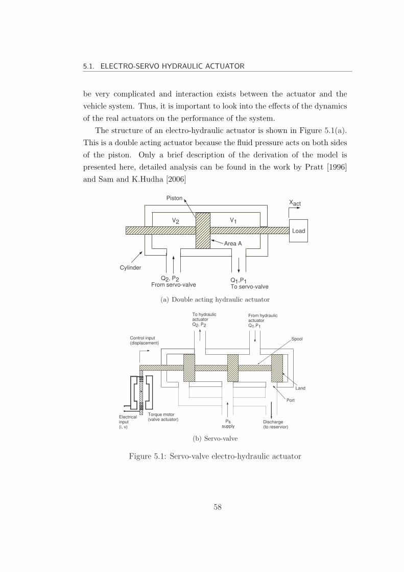
5.1. ELECTRO-SERVO HYDRAULIC ACTUATOR
be very complicated and interaction exists between the actuator and the
vehicle system. Thus, it is important to look into the effects of the dynamics
of the real actuators on the performance of the system.
The structure of an electro-hydraulic actuator is shown in Figure 5.1(a).
This is a double acting actuator because the fluid pressure acts on both sides
of the piston. Only a brief description of the derivation of the model is
presented here, detailed analysis can be found in the work by Pratt [1996]
and Sam and K.Hudha [2006]
xxxxxxxxxxxxxxxxxxxxxxxxxxxxxxxxxxxxxxxxxxxxxxx
xxxxxxxxx
xxxxxxxxxxxxxxxxxxxxxxxxxxxxxxxxxxxxxxxxxx
xxxxxx
xxxxxxxxxxxx
xxxxxxxxxx
xxxxxxxxx
xxxxxxxxx
xxxx
xxxxxx
xxxxxx
xxxx
xxx
xxxxxxxxx
xxxxxx
xxxxxxx
xxxx
xxxxxxxxxx
xxxxxxxxxxxxxxxxxxxxxxxxxxxxxxxxxxxxxxxxxxxxxxxxxxxxxxxxxxxxxxxxxxxxxxxxxxxxxxxxxxxxxxxxxxxxxxxxxx
xxxxxxxxxxxxxxxxxxxxxxxxxxxxxxxxxxxxxxxxxxxxxxxxxxxxxxxxxxxxxxxxxxxxxxxxxxxxxxxxxxxxxxxxxxxxxxxxxxxxxxxxxxxxxxxxxxxxxxxxxxxx
xxxxxxxxxxxxxxxxxxxxxxxxxxxxxxxxxxxxxxxxxxxxxxxxxxxxxxxxxxxxxxxxxxxxxxxxxxxxxxxxxxxxxxxxxxxxxxxxxxxxxxxxxxxx
Load
Q2, P2From servo-valve
Q1,P1To servo-valve
Cylinder
Xact
V2 V1
Area A
Piston
(a) Double acting hydraulic actuator
xxxxxxxxx
xxxxxx
xxxxxxxxx
xxxxxxx
xxxxxxxxxxxxxxxxxxxxxxxxxxxxxxxxxxxxxxxxxxxxxxxxxxxxxxxxxxxxxxxxxxxxxxxxxxxxxxxxxxxxxxxxxxxxxxxxxxxxxxxxx
xxxxxxxxxxxxxxxxxxxxxxxxxxxxxxxxxxxxxxxxxxxxxxxxxxxxxxxxxxxxxxxxxxxxxxxxxxxxxxxxxxxxxxxxxxxxxxxxxxxxxxxxx
xxxxxxxxxxxxxxxxxxxxxxxxxxxxxxxxxxxxxxxxxxxxxxxxxxxxxxxxxxxxxxxxxxxxxxxxxxxxxxxxxxxxxxxxxx
xxxxxxxxxxxxxxxxxxxxxxxxxxxxxxxxxxxxxxxxxxxxxxxxxxxxxxxxxxxxxxxxxxxxx
xxxxxxxxxxxxxxxxxxxxxxxxxxxxxxxxxxxxxxxxxxxxxxxxxxx
xxxxxxxxxxxxxxxxxxxxxxxxxxxxxxxxxxxxxxxxxxxxxxxxxxx
xxxxxxxxxxxxxxxxxxxxxxxxxxxxxxxxxxxxxxxxxxxxxxxxxxxxxxxxxxxxxxxxxxxxx
xxxxxxxx
Pssupply
Discharge(to reservior)
Torque motor(valve actuator)
To hydraulicactuatorQ2, P2
From hydraulicactuatorQ1,P1
Electricalinput(i, v)
Spool
Port
Control input(displacement)
Land
(b) Servo-valve
Figure 5.1: Servo-valve electro-hydraulic actuator
58

5.1. ELECTRO-SERVO HYDRAULIC ACTUATOR
5.1.1 Spool valve
The fluid flow Q1 and Q2 are controlled by the spool-valve as is shown in
Figure 5.1(b).
Q2 = xvbcd
√2(Ps − P2)
ρ(5.1)
Q1 = xvbcd
√2P1
ρ(5.2)
where xv is the spool valve displacement. b is the land width, cd is the
discharge coefficient at each port, ρ is the density of the hydraulic fluid, and
Ps is the supply pressure of the hydraulic fluid. The pressure at the discharge
end is taken to be zero.
For small displacement about the operating point, the following linearized
equations (5.1) and (5.2) can be given
δQ1 = kq1δxv − kc1δP1 (5.3)
δQ2 = kq2δxv + kc2δP2 (5.4)
where kq1 and kq2 are the flow gains
kq1 =
(∂Q1
∂xv
)|P1
kq2 =
(∂Q2
∂xv
)|P2
and kc1 and kc2 are the flow pressure coefficients
kc1 =
(∂Q1
∂P1
)|xv
kc2 =
(∂Q2
∂P2
)|xv
59

5.1. ELECTRO-SERVO HYDRAULIC ACTUATOR
5.1.2 Hydraulic primary actuator
The flow rate at the ports of a hydraulic actuator is regulated typically by
a spool valve. The flow rate of Q into a chamber depends primarily on two
factors:
1. Increase in chamber volume
2. Increase in pressure. Assuming that there is no leakage in the flow
the fluid conservation (i.e flow continuity ) equations can be written as
Q1 = Adxact
dt− V1
β
dP1
dt(5.5)
Q2 = Adxact
dt+
V2
β
dP2
dt(5.6)
Equation (5.5) and (5.6) are associated with the annulus side and the bore
side of the cylinder respectively. Q1 and Q2 are the flow rates. P1 and P2 are
the oil pressures. V1 and V2 are the oil volumes. xact is the is the extension
of the actuator. β is the bulk modulus.
For incremental changes about the operating point, equation (5.5) and
(5.6) can be written as
δQ1 = Adδxact
dt− V1
β
dδP1
dt(5.7)
δQ2 = Adδxact
dt+
V2
β
dδP2
dt(5.8)
where V1 and V2 are the oil volumes about the operating point.
In a linear model, the incremental-value given by equations 5.7 and 5.8
are used instead of the total-value equations 5.5 and 5.6. Equating cylinder
oil flows given by equations (5.7) and (5.8) with the spool-valve flows given
by equations (5.3) and (5.4) gives
Adδxact
dt− V1
β
dδP1
dt= kqδxv − kcδP1 (5.9)
Adδxact
dt+
V2
β
dδP2
dt= kqδxv + kcδP2 (5.10)
60
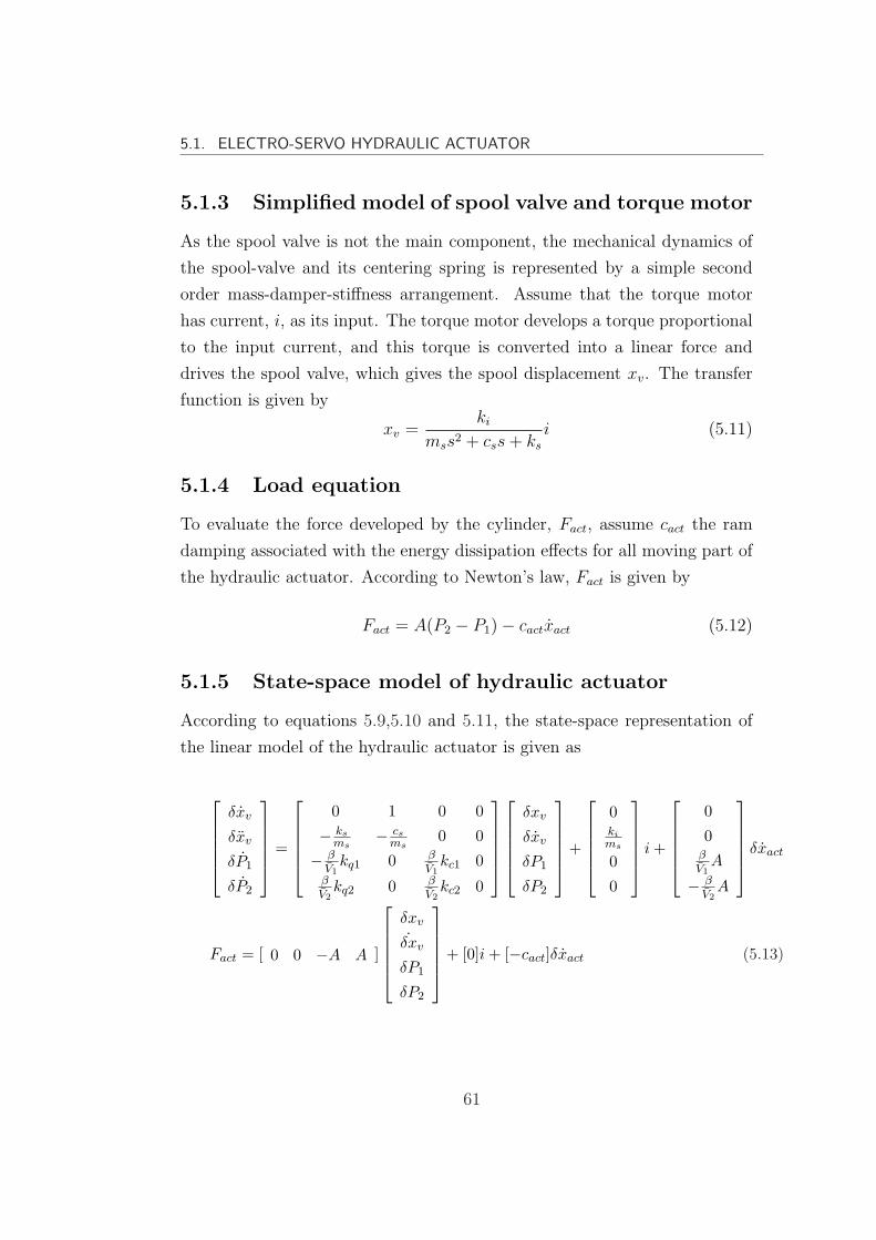
5.1. ELECTRO-SERVO HYDRAULIC ACTUATOR
5.1.3 Simplified model of spool valve and torque motor
As the spool valve is not the main component, the mechanical dynamics of
the spool-valve and its centering spring is represented by a simple second
order mass-damper-stiffness arrangement. Assume that the torque motor
has current, i, as its input. The torque motor develops a torque proportional
to the input current, and this torque is converted into a linear force and
drives the spool valve, which gives the spool displacement xv. The transfer
function is given by
xv =ki
mss2 + css + ks
i (5.11)
5.1.4 Load equation
To evaluate the force developed by the cylinder, Fact, assume cact the ram
damping associated with the energy dissipation effects for all moving part of
the hydraulic actuator. According to Newton’s law, Fact is given by
Fact = A(P2 − P1)− cactxact (5.12)
5.1.5 State-space model of hydraulic actuator
According to equations 5.9,5.10 and 5.11, the state-space representation of
the linear model of the hydraulic actuator is given as
δxv
δxv
δP1
δP2
=
0 1 0 0
− ksms
− csms
0 0
− βV1
kq1 0 βV1
kc1 0βV2
kq2 0 βV2
kc2 0
δxv
δxv
δP1
δP2
+
0kims
0
0
i +
0
0βV1
A
− βV2
A
δxact
Fact = [ 0 0 −A A ]
δxv
˙δxv
δP1
δP2
+ [0]i + [−cact]δxact (5.13)
61
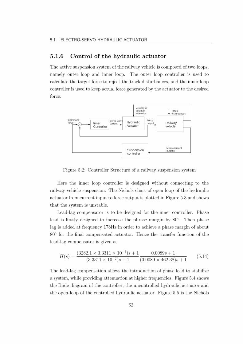
5.1. ELECTRO-SERVO HYDRAULIC ACTUATOR
5.1.6 Control of the hydraulic actuator
The active suspension system of the railway vehicle is composed of two loops,
namely outer loop and inner loop. The outer loop controller is used to
calculate the target force to reject the track disturbances, and the inner loop
controller is used to keep actual force generated by the actuator to the desired
force.
Railwayvehicle
HydraulicActuator
Inner Controller
Suspensioncontroller
Commandforce
Forceoutput
Trackdisturbances
Measurementoutputs
Velocity ofactuatorextension
Servo-valvecurrent
Figure 5.2: Controller Structure of a railway suspension system
Here the inner loop controller is designed without connecting to the
railway vehicle suspension. The Nichols chart of open loop of the hydraulic
actuator from current input to force output is plotted in Figure 5.3 and shows
that the system is unstable.
Lead-lag compensator is to be designed for the inner controller. Phase
lead is firstly designed to increase the phrase margin by 80. Then phase
lag is added at frequency 178Hz in order to achieve a phase margin of about
80 for the final compensated actuator. Hence the transfer function of the
lead-lag compensator is given as
H(s) =(3282.1× 3.3311× 10−7)s + 1
(3.3311× 10⁻⁷)s + 1
0.0089s + 1
(0.0089× 462.38)s + 1(5.14)
The lead-lag compensation allows the introduction of phase lead to stabilize
a system, while providing attenuation at higher frequencies. Figure 5.4 shows
the Bode diagram of the controller, the uncontrolled hydraulic actuator and
the open-loop of the controlled hydraulic actuator. Figure 5.5 is the Nichols
62
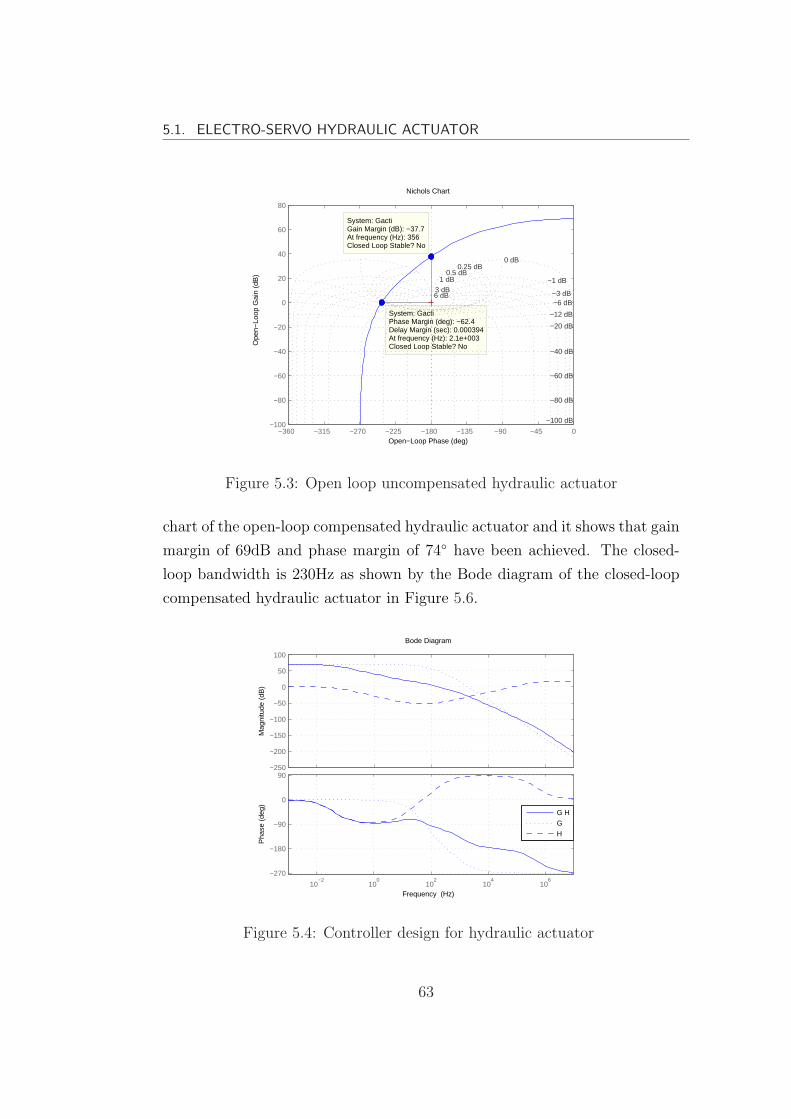
5.1. ELECTRO-SERVO HYDRAULIC ACTUATOR
Nichols Chart
Open−Loop Phase (deg)
Ope
n−Lo
op G
ain
(dB
)
−360 −315 −270 −225 −180 −135 −90 −45 0−100
−80
−60
−40
−20
0
20
40
60
80
System: GactiGain Margin (dB): −37.7At frequency (Hz): 356Closed Loop Stable? No
System: GactiPhase Margin (deg): −62.4Delay Margin (sec): 0.000394At frequency (Hz): 2.1e+003Closed Loop Stable? No
6 dB 3 dB
1 dB 0.5 dB
0.25 dB 0 dB
−1 dB
−3 dB −6 dB
−12 dB
−20 dB
−40 dB
−60 dB
−80 dB
−100 dB
Figure 5.3: Open loop uncompensated hydraulic actuator
chart of the open-loop compensated hydraulic actuator and it shows that gain
margin of 69dB and phase margin of 74 have been achieved. The closed-
loop bandwidth is 230Hz as shown by the Bode diagram of the closed-loop
compensated hydraulic actuator in Figure 5.6.
−250
−200
−150
−100
−50
0
50
100
Mag
nitu
de (
dB)
10−2
100
102
104
106
−270
−180
−90
0
90
Pha
se (
deg)
Bode Diagram
Frequency (Hz)
G H
G
H
Figure 5.4: Controller design for hydraulic actuator
63

5.1. ELECTRO-SERVO HYDRAULIC ACTUATOR
Open−loop of controlled hydraulic actuator
Open−Loop Phase (deg)
Ope
n−Lo
op G
ain
(dB
)
−270 −225 −180 −135 −90 −45 0−250
−200
−150
−100
−50
0
50
100
System: GopenPhase Margin (deg): 74.3Delay Margin (sec): 0.00115At frequency (Hz): 179Closed Loop Stable? Yes
System: GopenGain Margin (dB): 69.2At frequency (Hz): 2.07e+004Closed Loop Stable? Yes
Figure 5.5: Open loop of controlled hydraulic actuator
100
101
102
103
104
105
106
107
−270
−225
−180
−135
−90
−45
0
Pha
se (
deg)
Bode Diagram
Frequency (Hz)
−250
−200
−150
−100
−50
0
System: untitled1Frequency (Hz): 230Magnitude (dB): −3
Mag
nitu
de (
dB)
Figure 5.6: Closed-loop of controlled hydraulic actuator
64

5.1. ELECTRO-SERVO HYDRAULIC ACTUATOR
Figure 5.7 shows the time response of the closed-loop hydraulic actuator
to a square-wave force demand of 1kN at 10Hz. Figure 5.8 shows the ability
of the closed-loop system to reject a unit 1Hz square-wave disturbance placed
on the extension of the actuator given a zero force demand.
0 0.05 0.1 0.15 0.2 0.250
100
200
300
400
500
600
700
800
900
1000
10Hz force following
Time (sec)
For
ce(N
)
Figure 5.7: Closed-loop hydraulic actuator force following
0.5 1 1.5 2 2.5 3 3.5 4 4.5−2.5
−2
−1.5
−1
−0.5
0
0.5
1
1.5
2
x 104 1Hz disturbance rejection
Time (sec)
For
ce(N
)
Figure 5.8: Closed-loop hydraulic actuator disturbance rejection
65
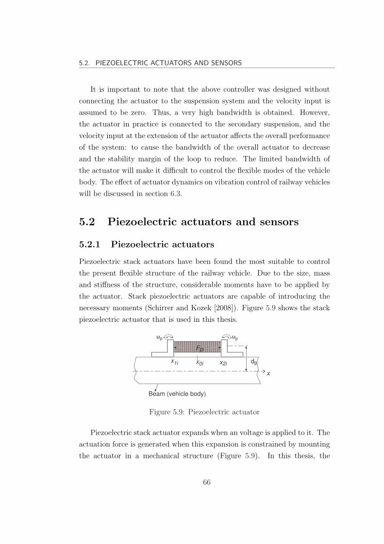
5.2. PIEZOELECTRIC ACTUATORS AND SENSORS
It is important to note that the above controller was designed without
connecting the actuator to the suspension system and the velocity input is
assumed to be zero. Thus, a very high bandwidth is obtained. However,
the actuator in practice is connected to the secondary suspension, and the
velocity input at the extension of the actuator affects the overall performance
of the system: to cause the bandwidth of the overall actuator to decrease
and the stability margin of the loop to reduce. The limited bandwidth of
the actuator will make it difficult to control the flexible modes of the vehicle
body. The effect of actuator dynamics on vibration control of railway vehicles
will be discussed in section 6.3.
5.2 Piezoelectric actuators and sensors
5.2.1 Piezoelectric actuators
Piezoelectric stack actuators have been found the most suitable to control
the present flexible structure of the railway vehicle. Due to the size, mass
and stiffness of the structure, considerable moments have to be applied by
the actuator. Stack piezoelectric actuators are capable of introducing the
necessary moments (Schirrer and Kozek [2008]). Figure 5.9 shows the stack
piezoelectric actuator that is used in this thesis.
xxxxxxxxxxxxxxxxxxxxxxxxxxxxxxxxxxxxxxxxxxxxxxxxxxxxxxxxxxxxxxxxxxxxxxxxxxxxxxxxxxxxxxxxxxxxxxxxxxxxxxxxxxxxxxxxxxxxxxxxxxxxxxxxxxxxxxxxxxxxxxxxxxxxxxxxxxxxxxxxxxxxxxxxxxxxxxxxxxxxxx
xxxxx xxxxxFp
xxxxxxxxxxxxxxxxxxxxxxxxxxxxxxxxxxxxxxxxxxxxxxxxxxxxxxxxxxxxxxxxxxxxx x
x1i x2ixxxxxxxxxxx
dp
MpMp
x0i
xxxxxxxxxxxxxx
xxxxxxxxx
xxxx
xxxxxxx
xxxxxxxxxxxx
Beam (vehicle body)
xxxxxxxxxxxxxx
xxxxxxxxx
xxx x
xxxxxxx
xxxxxxxxxxxx
Figure 5.9: Piezoelectric actuator
Piezoelectric stack actuator expands when an voltage is applied to it. The
actuation force is generated when this expansion is constrained by mounting
the actuator in a mechanical structure (Figure 5.9). In this thesis, the
66
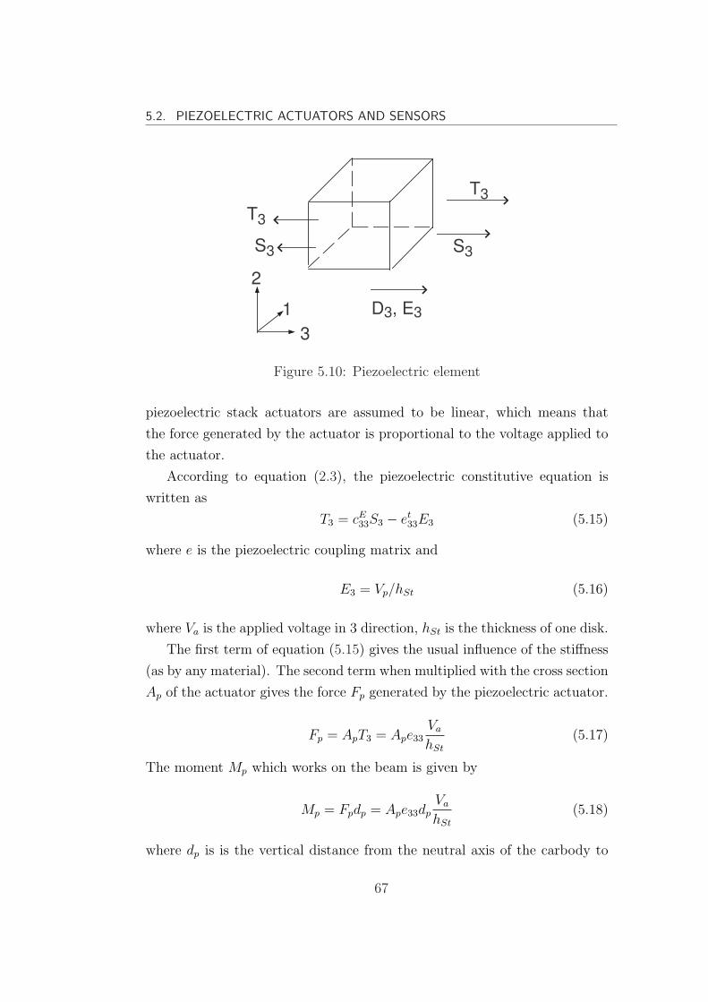
5.2. PIEZOELECTRIC ACTUATORS AND SENSORS
T3
S3
T3
S3
2
1
3
D3, E3
Figure 5.10: Piezoelectric element
piezoelectric stack actuators are assumed to be linear, which means that
the force generated by the actuator is proportional to the voltage applied to
the actuator.
According to equation (2.3), the piezoelectric constitutive equation is
written as
T3 = cE33S3 − et
33E3 (5.15)
where e is the piezoelectric coupling matrix and
E3 = Vp/hSt (5.16)
where Va is the applied voltage in 3 direction, hSt is the thickness of one disk.
The first term of equation (5.15) gives the usual influence of the stiffness
(as by any material). The second term when multiplied with the cross section
Ap of the actuator gives the force Fp generated by the piezoelectric actuator.
Fp = ApT3 = Ape33Va
hSt
(5.17)
The moment Mp which works on the beam is given by
Mp = Fpdp = Ape33dpVa
hSt
(5.18)
where dp is is the vertical distance from the neutral axis of the carbody to
67

5.2. PIEZOELECTRIC ACTUATORS AND SENSORS
the vertical centre of the piezoelectric actuator. Hence the coefficient Ka in
equation (4.35) is given as
Ka = Ape33dp/hSt (5.19)
Detailed working principle of the piezoelectric actuator was not included
above. In this thesis, it is concentrated on the active vibration control of the
flexible vehicle body with active damping by piezoelectric actuators, so it is
only important to use an actuator with a linear input/output relation and
sufficient dynamics.
5.2.2 Piezoelectric sensors
Piezoelectric patches are used as sensors. They are bonded to the structure
and produce a voltage signal that is proportional to the average curvature.
The measurements by piezoelectric sensors, in comparison to position,
velocity and acceleration measurements, is advantageous when only the
vibrations of the flexible modes have to be measured and the signal part
of the rigid body modes has to be eliminated (Benatzky et al.).
The vibration of the beam will induce strain inside the beam element.
This strain will then induce an electric charge inside the piezoelectric sensor
due to the piezoelectric effect. The charge Q and the voltage vpj generated
across the sensor electrodes, are related by the capacitance of the sensor, Cp
vpj = Q/Cp (5.20)
The induced voltage vpj by the jth piezoelectric sensor is given by (Halim
[2002])
vpj(t) =Ks
Cp
∞∑r=1
Ψrjqr(t) (5.21)
where
Ψrj =dφr
dx(x2j)− dφr
dx(x1j) (5.22)
Equation (5.21) implies that the jth sensor output consists of the
68
5.3. PLACEMENT OF ACTUATORS AND SENSORS
contribution of each bending mode, where the contribution of each mode
is proportional to Ψrj (Halim and Moheimani [2001]).
5.3 Placement of actuators and sensors
The placement of piezoelectric actuators and sensors on a flexible structure
for active vibration suppression is a crucial issue because it has an direct effect
on the achievable performance. The controllability and observability of the
flexible modes vary as the positions of the actuators and sensors changes. A
flexible mode cannot be controlled by the actuator placed at the node point
of the mode. Moreover, if the sensor is placed at one of the nodes, then no
control of the mode is possible, even if the actuator is not co-located. In this
thesis, the placement of actuators and sensors are determined based on the
H2 and H∞ norms of the flexible structures (Gawronski [1998]).
5.3.1 Norms of a flexible structure
For a continuous-time system G(ω), the H2 norm of the system is defined as
‖G‖22 =
1
2π
∫ ∞
−∞tr(G∗(ω)G(ω))dω (5.23)
where tr(G∗(ω)G(ω)) is the sum of the squared magnitudes of all the elements
of G(ω). Thus the H2 norm can be interpreted as an average gain of the
system, performed over all the elements of the matrix transfer function and
over all frequencies.
The H∞ norm is defined as
‖G‖∞ = maxω
σmax(G(ω)) (5.24)
where σmax(G(ω)) is the largest singular value of G(ω). H∞ norm is the
worst case gain for sinusoidal inputs at any frequency.
The equations of a flexible structure are uncoupled in modal coordinates
and the system norms can be decomposed to a combination of single-input-
69

5.3. PLACEMENT OF ACTUATORS AND SENSORS
single-output norms. The norms of the rth mode and ith actuator and jth
sensor can be approximately determined from
‖Grij‖2∼= ‖bri‖2‖crj‖2
2√
ζrωr
(5.25)
‖Grij‖∞ ∼= ‖bri‖2‖crj‖2
2ζrωr
(5.26)
where 2ζrωr is defined as a half-power frequency at the rth resonance (Clough
and Penzien [1975] and Ewins [2000]). (The interested audience can refer to
Gawronski [1998] for the proof of equation (5.25) and (5.26)). The entries
of input matrix bri and output matrix crj are dependent on the locations of
actuators and sensors, respectively.
For a flexible structure with a set of np actuators and mp sensors, the H2
(or H∞) norm of the rth mode is the root-mean-square sum over all actuators
and sensors, which are the additive properties for the H2 and H∞ norms with
a set of actuators and sensors for a mode:
The H2 norm of the rth mode can be approximately determined by
‖Gr‖2∼=
np∑i=1
mp∑j=1
‖Grij‖2 (5.27)
And the H∞ norm of the rth mode can be approximately determined by
‖Gr‖∞ ∼=np∑i=1
mp∑j=1
‖Grij‖∞ (5.28)
The H2 norm of the total system is approximately the root-mean-square
sum over all its modal norms, that is
‖G‖2∼=
n∑r=1
‖Gr‖2 (5.29)
where n is the number of modes taken under consideration.
TheH∞ norm of the total system is approximately the largest of its modal
70
5.3. PLACEMENT OF ACTUATORS AND SENSORS
norms
‖G‖∞ ∼= maxr‖Gr‖∞ (5.30)
The properties presented by equations 5.25 to 5.30 are very useful
for evaluating the importance of an arbitrary combination of sensors and
actuators and are applicable to structures only, because in general case,
system norms cannot be decomposed into a combination of single-input-
single-output norms.
5.3.2 Placement indices
The placement indices are defined as
σ2rij =‖Grij‖2
‖Gr‖2
(5.31)
σ∞rij =‖Grij‖∞‖Gr‖∞ (5.32)
Placement indices σ2rij /σ∞rij is a measure of the contribution of the ith
actuator and jth sensor in the impulse response of the rth mode.
Based on the definition for the placement indices by equation (5.31) and
(5.32), the actuator/sensor placement problem is stated as: given a larger
set of sensors and actuator (which are the possible mounting positions for
actuators and sensors), determine the locations of a smaller subset of sensors
or actuators such that the H2 or H∞ norms of the subset are as close as
possible to the norms of the original set.
5.3.3 Placement of actuators and sensors for flexible
body of a railway vehicle
Modal model
np piezoelectric actuators and mp piezoelectric sensors are to be attached
onto the vehicle body. For the placement of the actuators and sensors, the
modal model of the railway vehicle body given by equations (4.40) and (4.41)
is used. This model considers only the first two flexible modes and disregards
71
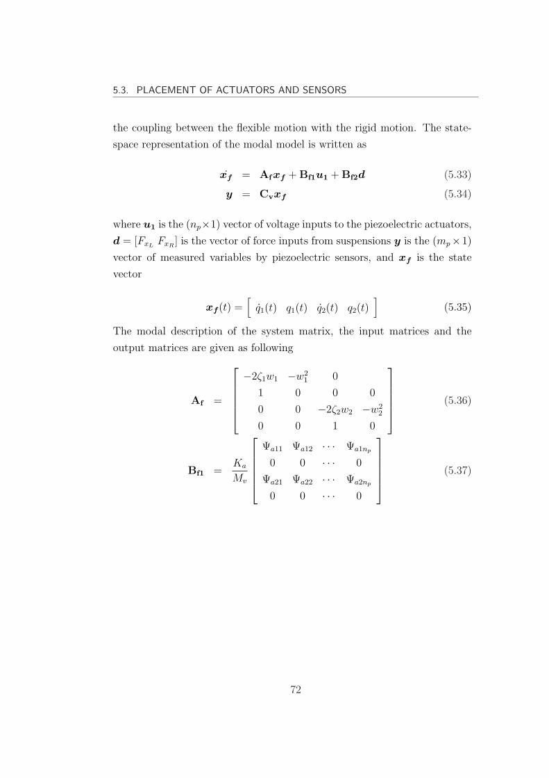
5.3. PLACEMENT OF ACTUATORS AND SENSORS
the coupling between the flexible motion with the rigid motion. The state-
space representation of the modal model is written as
xf = Afxf + Bf1u1 + Bf2d (5.33)
y = Cvxf (5.34)
where u1 is the (np×1) vector of voltage inputs to the piezoelectric actuators,
d = [FxLFxR
] is the vector of force inputs from suspensions y is the (mp×1)
vector of measured variables by piezoelectric sensors, and xf is the state
vector
xf (t) =[
q1(t) q1(t) q2(t) q2(t)]
(5.35)
The modal description of the system matrix, the input matrices and the
output matrices are given as following
Af =
−2ζ1w1 −w21 0
1 0 0 0
0 0 −2ζ2w2 −w22
0 0 1 0
(5.36)
Bf1 =Ka
Mv
Ψa11 Ψa12 · · · Ψa1np
0 0 · · · 0
Ψa21 Ψa22 · · · Ψa2np
0 0 · · · 0
(5.37)
72

5.3. PLACEMENT OF ACTUATORS AND SENSORS
Bf2 =
φ1(xL)Mv
φ1(xR)Mv
0 0φ2(xL)
Mv
φ2(xR)Mv
0 0
(5.38)
Cv =Ks
Cp
0 Ψs11 0 Ψs21
0 Ψs12 0 Ψs22
0... 0
...
0 Ψs1mp 0 Ψs2mp
(5.39)
where Ψari is the coefficient of the ith actuator for the rth mode, and Ψsrj is
the coefficient of the jth sensors for the rth mode. They are functions of the
position of the actuator/sensor (denoted by the centre of the actuator/sensor,
x) and the length of the actuator/sensor,Lp.
Candidate positions
According to the definition of the structural norms, placement indices and the
input and output matrices given by equations (5.38) to (5.39), the placement
of the piezoelectric actuators and sensors is closely related to the absolute
values of Ψa and Ψs, i.e. at the position where Ψari and Ψsrj have high
absolute values, the placement indices will also have high values and vice
versa.
With the length of the piezoelectric actuator and sensor fixed, the plot
of Ψa(x) of a single actuator is shown in Figure 5.11. The absolute value
of Ψa(x) reaches its maxima at abdominal positions of the plot: x = (13.5)
for the 1st flexible mode, and x = (7.84) and x = (19.16) for the 2nd flexible
mode, where x is the coordinate. It is found Ψa2(13.5) = 0, which means
centre of the vehicle body is the node point for the second flexible mode, and
the second flexible mode can not controlled by piezoelectric actuators placed
at x = (13.5).
With the location of sensors fixed, the plot of normalized H2 indices and
H∞ indices as a function of actuator locations, x, are shown in Figures 5.12
and 5.13. It is not surprising to find that the maxima positions in H∞/H2
73
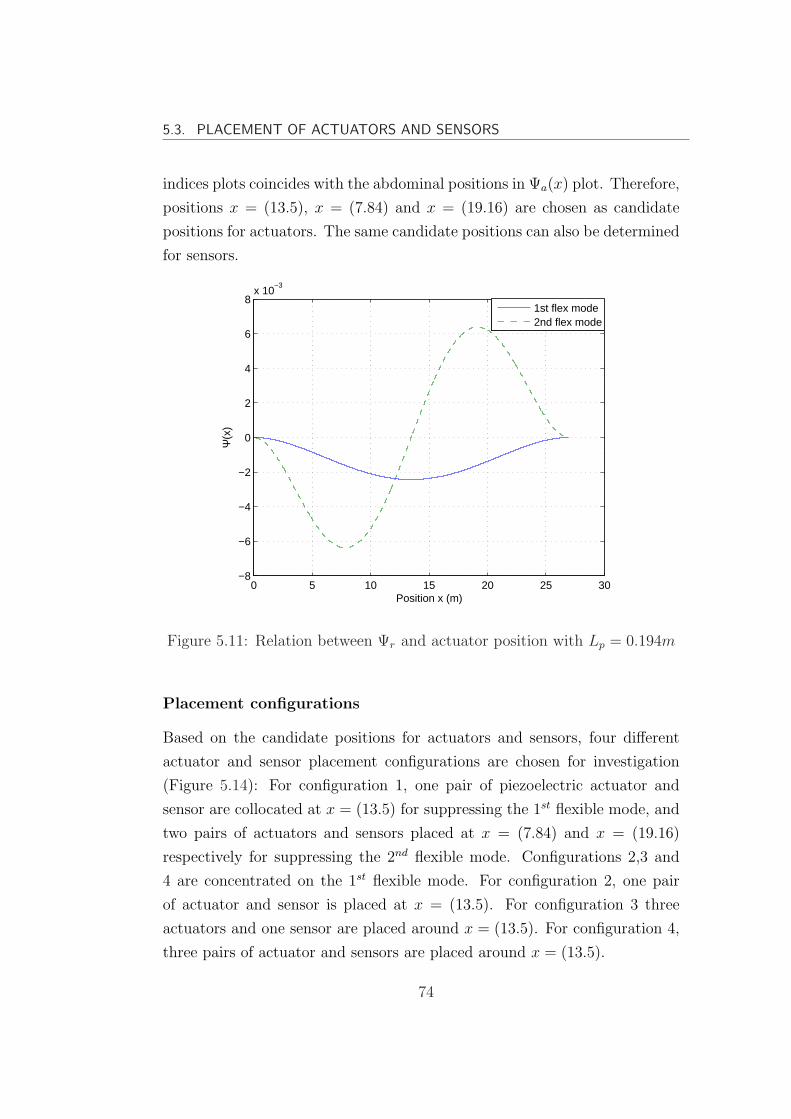
5.3. PLACEMENT OF ACTUATORS AND SENSORS
indices plots coincides with the abdominal positions in Ψa(x) plot. Therefore,
positions x = (13.5), x = (7.84) and x = (19.16) are chosen as candidate
positions for actuators. The same candidate positions can also be determined
for sensors.
0 5 10 15 20 25 30−8
−6
−4
−2
0
2
4
6
8x 10
−3
Position x (m)
Ψ(x
)
1st flex mode2nd flex mode
Figure 5.11: Relation between Ψr and actuator position with Lp = 0.194m
Placement configurations
Based on the candidate positions for actuators and sensors, four different
actuator and sensor placement configurations are chosen for investigation
(Figure 5.14): For configuration 1, one pair of piezoelectric actuator and
sensor are collocated at x = (13.5) for suppressing the 1st flexible mode, and
two pairs of actuators and sensors placed at x = (7.84) and x = (19.16)
respectively for suppressing the 2nd flexible mode. Configurations 2,3 and
4 are concentrated on the 1st flexible mode. For configuration 2, one pair
of actuator and sensor is placed at x = (13.5). For configuration 3 three
actuators and one sensor are placed around x = (13.5). For configuration 4,
three pairs of actuator and sensors are placed around x = (13.5).
74
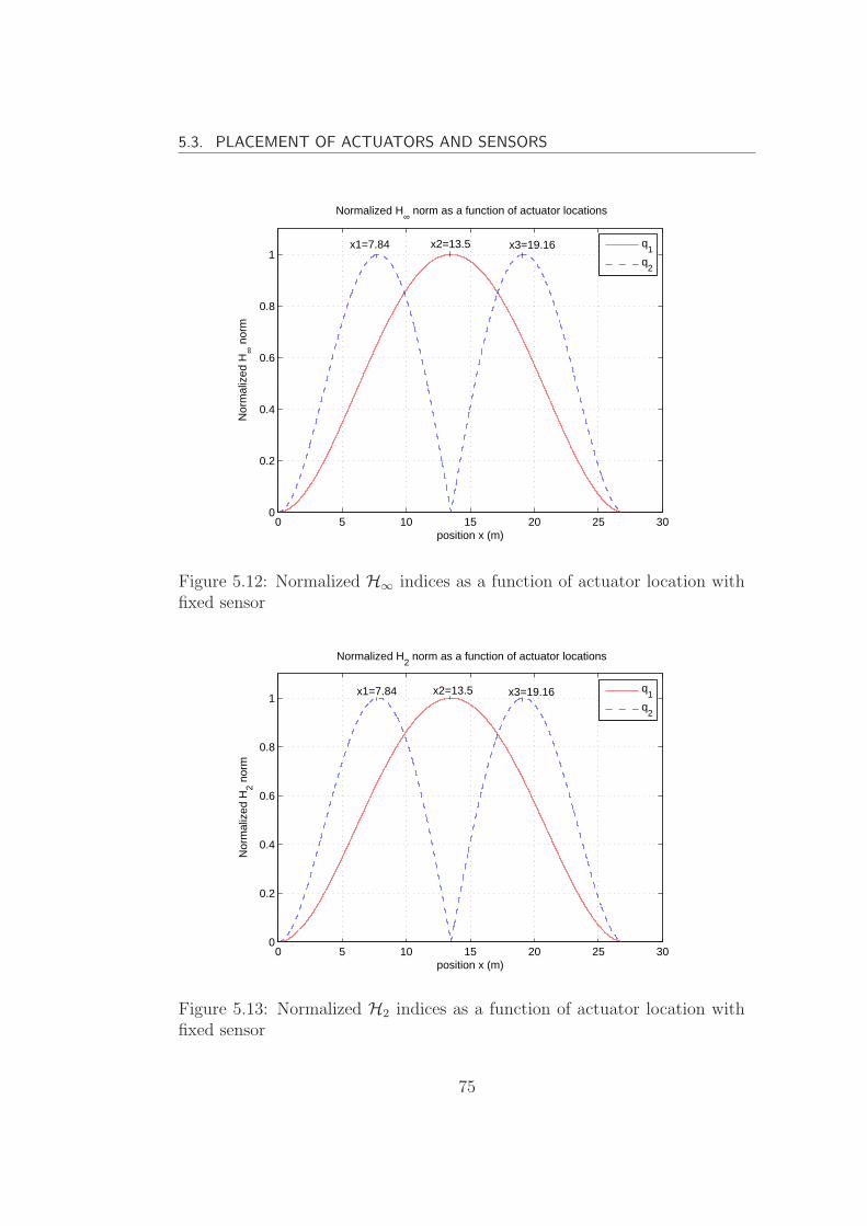
5.3. PLACEMENT OF ACTUATORS AND SENSORS
0 5 10 15 20 25 300
0.2
0.4
0.6
0.8
1
position x (m)
Nor
mal
ized
H∞
nor
m
Normalized H∞ norm as a function of actuator locations
q
1
q2
x1=7.84 x2=13.5 x3=19.16
Figure 5.12: Normalized H∞ indices as a function of actuator location withfixed sensor
0 5 10 15 20 25 300
0.2
0.4
0.6
0.8
1
position x (m)
Nor
mal
ized
H2 n
orm
Normalized H2 norm as a function of actuator locations
q
1
q2
x2=13.5x1=7.84 x3=19.16
Figure 5.13: Normalized H2 indices as a function of actuator location withfixed sensor
75
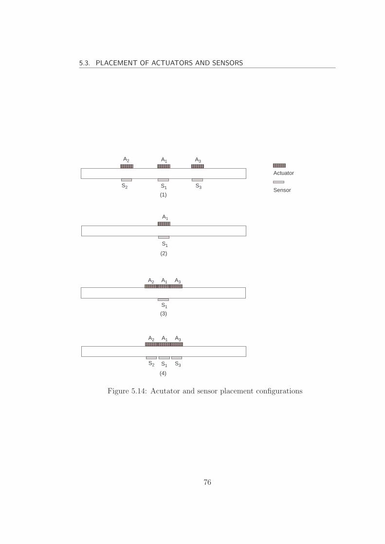
5.3. PLACEMENT OF ACTUATORS AND SENSORS
xxxxxxxxxxxxxxxxxxxxx
xxxxxxxxxxxxxxxxxxxxx
xxxxxxxxxxxxxxxxxxxxx
xxxxxxxxxxxxxxxxxxxxx
xxxxxxxxxxxxxxxxxxxxxxxx
xxxxxxxxxxxxxxxxxxxxx
xxxxxxxxxxxxxxxxxxxxx
xxxxxxxxxxxxxxxxxxxxx
xxxxxxxxxxxxxxxxxxxxx
xxxxxxxxxxxxxxxxxxxxx
xxxxxxxxxxxxxxxxxxxxx
Actuator
Sensor
A2 A1 A3
S2 S1 S3
A1
S1
S1
A1A2 A3
A1A2 A3
S2 S1 S3
(1)
(2)
(3)
(4)
Figure 5.14: Acutator and sensor placement configurations
76
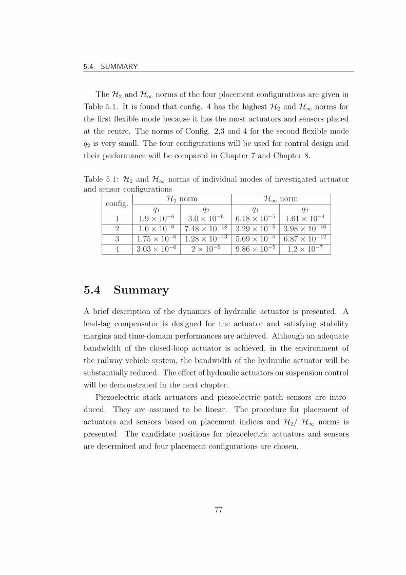
5.4. SUMMARY
The H2 and H∞ norms of the four placement configurations are given in
Table 5.1. It is found that config. 4 has the highest H2 and H∞ norms for
the first flexible mode because it has the most actuators and sensors placed
at the centre. The norms of Config. 2,3 and 4 for the second flexible mode
q2 is very small. The four configurations will be used for control design and
their performance will be compared in Chapter 7 and Chapter 8.
Table 5.1: H2 and H∞ norms of individual modes of investigated actuatorand sensor configurations
config.H2 norm H∞ norm
q1 q2 q1 q2
1 1.9× 10⁻⁶ 3.0× 10⁻⁶ 6.18× 10⁻⁵ 1.61× 10⁻⁴
2 1.0× 10⁻⁶ 7.48× 10⁻¹⁸ 3.29× 10⁻⁵ 3.98× 10⁻¹⁶
3 1.75× 10⁻⁶ 1.28× 10⁻¹³ 5.69× 10⁻⁵ 6.87× 10⁻¹²
4 3.03× 10⁻⁶ 2× 10⁻⁹ 9.86× 10⁻⁵ 1.2× 10⁻⁷
5.4 Summary
A brief description of the dynamics of hydraulic actuator is presented. A
lead-lag compensator is designed for the actuator and satisfying stability
margins and time-domain performances are achieved. Although an adequate
bandwidth of the closed-loop actuator is achieved, in the environment of
the railway vehicle system, the bandwidth of the hydraulic actuator will be
substantially reduced. The effect of hydraulic actuators on suspension control
will be demonstrated in the next chapter.
Piezoelectric stack actuators and piezoelectric patch sensors are intro-
duced. They are assumed to be linear. The procedure for placement of
actuators and sensors based on placement indices and H2/ H∞ norms is
presented. The candidate positions for piezoelectric actuators and sensors
are determined and four placement configurations are chosen.
77
Chapter 6
Preliminary Studies with
Active Suspension Control
This chapter describes the design of active suspension control for improving
the ride quality of railway vehicles. Two control approaches, modal control
with skyhook damping and LQG control, are applied. It is aimed to
investigate the influences of flexibility of the vehicle body on the performance
of the designed controllers. For the model based approach of the LQG control,
both the rigid model and the flexible model are used as design models for
control design and the performance of the resulting controllers are compared.
Finally the effect of actuator dynamics upon the ride quality of the railway
vehicle with the designed controller is examined. Structural damping via
piezoelectric actuation is excluded in this chapter and will be added to control
design in Chapter 7 and Chapter 8.
6.1 Modal control with skyhook damping
The classical control method of skyhook damping is advantageous over
passive damping because the trade-off between resonance attenuation and
high frequency transmissibility has been eased. It is a simple method known
to give excellent improvements in ride quality of railway vehicles.
78
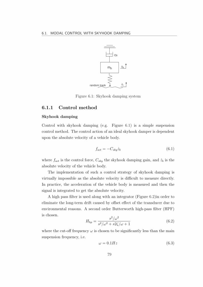
6.1. MODAL CONTROL WITH SKYHOOK DAMPING
mb
cs
random track zt
zb
Figure 6.1: Skyhook damping system
6.1.1 Control method
Skyhook damping
Control with skyhook damping (e.g. Figure 6.1) is a simple suspension
control method. The control action of an ideal skyhook damper is dependent
upon the absolute velocity of a vehicle body.
fact = −Cskyzb (6.1)
where fact is the control force, Csky the skyhook damping gain, and zb is the
absolute velocity of the vehicle body.
The implementation of such a control strategy of skyhook damping is
virtually impossible as the absolute velocity is difficult to measure directly.
In practice, the acceleration of the vehicle body is measured and then the
signal is integrated to get the absolute velocity.
A high pass filter is used along with an integrator (Figure 6.2)in order to
eliminate the long-term drift caused by offset effect of the transducer due to
environmental reasons. A second order Butterworth high-pass filter (HPF)
is chosen.
Hhp =s2/ω2
s2/ω2 + s2ζ/ω + 1(6.2)
where the cut-off frequency ω is chosen to be significantly less than the main
suspension frequency, i.e.
ω = 0.1Hz (6.3)
79

6.1. MODAL CONTROL WITH SKYHOOK DAMPING
mb
random track
zt
zb
1/s HPF
-cs
ForceActuator
F
Zb Zb
Figure 6.2: Intuitive control configuration: skyhook damping
and the damping ratio ζ and is chosen as
ζ = 70% (6.4)
Then the combined transfer function of the integrator and the HPF is given
by
Gint =2.533s
2.533s2 + 2.228s + 1(6.5)
Hence
ˆzb = Gintzb (6.6)
It provides the estimation of a velocity from the measured acceleration.
Modal control
Modal control attempts to manage individual modes of the system. The
measurement signals are decomposed into modal components, then the modal
components are processed individually, and finally they are recombined and
feed to the actuators. Figure 6.3 illustrates the structure of modal control
for the railway vehicle.
6.1.2 Control design
The structure of the control system is shown in Figure 6.4 Two linear
accelerometers are placed above the secondary suspensions at the left (xL)
and right (xR) of the vehicle for measuring the body accelerations: ZxLand
80
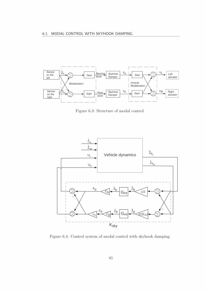
6.1. MODAL CONTROL WITH SKYHOOK DAMPING
Gain
Gain
Sensoron theleft
Sensoron theright
Gain
Gain
Bounceacce
Pitchacce
Skyhook Damper
Modalization InverseModalization
Left actuator
Right actuator
UL
UR
Fb
Fp
ZxL
ZxR Skyhook
Damper
Figure 6.3: Structure of modal control
1/2
UL
UR
Fb
Fp
ZxL
ZxR
Ksky
Cb
Cp 1/(2Lc)
Gint
GintLcZp
Vehicle dynamics
Z0L
Z0R
ZbZb
Zp
Figure 6.4: Control system of modal control with skyhook damping
81
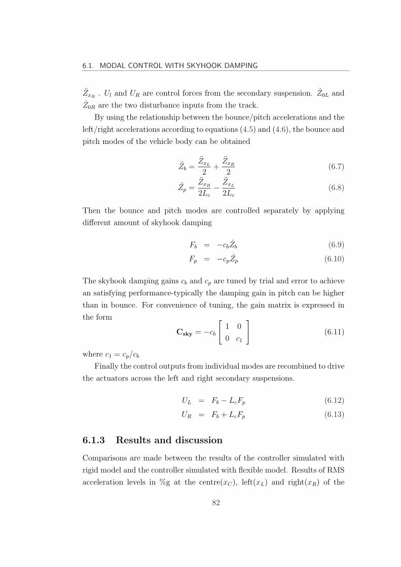
6.1. MODAL CONTROL WITH SKYHOOK DAMPING
ZxR. Ul and UR are control forces from the secondary suspension. Z0L and
Z0R are the two disturbance inputs from the track.
By using the relationship between the bounce/pitch accelerations and the
left/right accelerations according to equations (4.5) and (4.6), the bounce and
pitch modes of the vehicle body can be obtained
Zb =ZxL
2+
ZxR
2(6.7)
Zp =ZxR
2Lc
− ZxL
2Lc
(6.8)
Then the bounce and pitch modes are controlled separately by applying
different amount of skyhook damping
Fb = −cbZb (6.9)
Fp = −cpZp (6.10)
The skyhook damping gains cb and cp are tuned by trial and error to achieve
an satisfying performance-typically the damping gain in pitch can be higher
than in bounce. For convenience of tuning, the gain matrix is expressed in
the form
Csky = −cb
[1 0
0 c1
](6.11)
where c1 = cp/cb
Finally the control outputs from individual modes are recombined to drive
the actuators across the left and right secondary suspensions.
UL = Fb − LcFp (6.12)
UR = Fb + LcFp (6.13)
6.1.3 Results and discussion
Comparisons are made between the results of the controller simulated with
rigid model and the controller simulated with flexible model. Results of RMS
acceleration levels in %g at the centre(xC), left(xL) and right(xR) of the
82
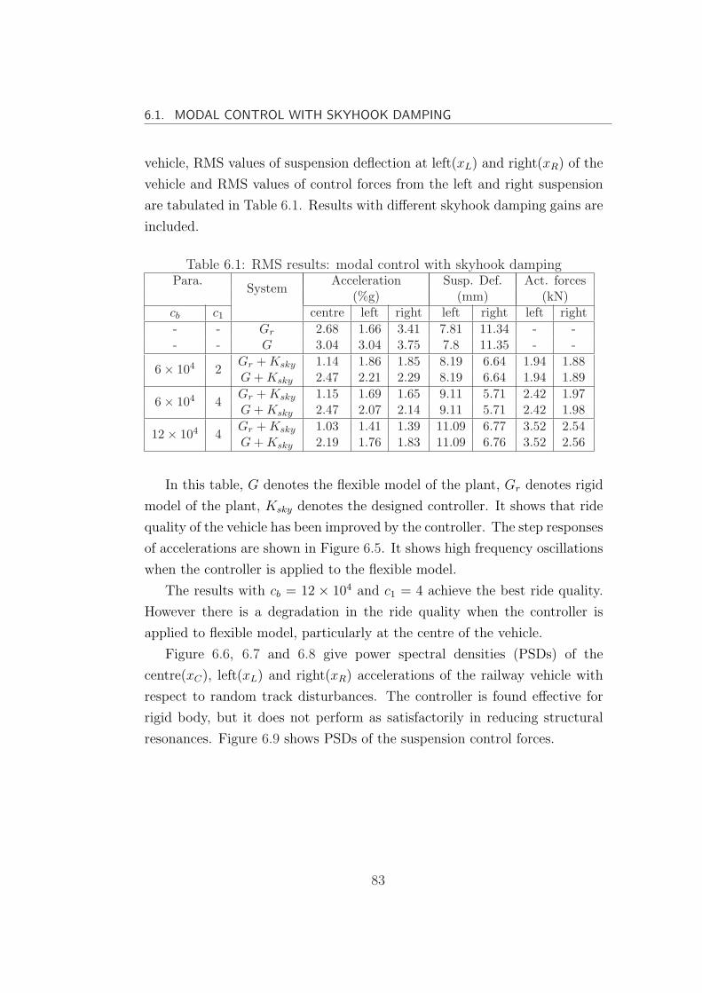
6.1. MODAL CONTROL WITH SKYHOOK DAMPING
vehicle, RMS values of suspension deflection at left(xL) and right(xR) of the
vehicle and RMS values of control forces from the left and right suspension
are tabulated in Table 6.1. Results with different skyhook damping gains are
included.
Table 6.1: RMS results: modal control with skyhook dampingPara.
SystemAcceleration Susp. Def. Act. forces
(%g) (mm) (kN)cb c1 centre left right left right left right- - Gr 2.68 1.66 3.41 7.81 11.34 - -- - G 3.04 3.04 3.75 7.8 11.35 - -
6× 10⁴ 2Gr + Ksky 1.14 1.86 1.85 8.19 6.64 1.94 1.88G + Ksky 2.47 2.21 2.29 8.19 6.64 1.94 1.89
6× 10⁴ 4Gr + Ksky 1.15 1.69 1.65 9.11 5.71 2.42 1.97G + Ksky 2.47 2.07 2.14 9.11 5.71 2.42 1.98
12× 104 4Gr + Ksky 1.03 1.41 1.39 11.09 6.77 3.52 2.54G + Ksky 2.19 1.76 1.83 11.09 6.76 3.52 2.56
In this table, G denotes the flexible model of the plant, Gr denotes rigid
model of the plant, Ksky denotes the designed controller. It shows that ride
quality of the vehicle has been improved by the controller. The step responses
of accelerations are shown in Figure 6.5. It shows high frequency oscillations
when the controller is applied to the flexible model.
The results with cb = 12 × 104 and c1 = 4 achieve the best ride quality.
However there is a degradation in the ride quality when the controller is
applied to flexible model, particularly at the centre of the vehicle.
Figure 6.6, 6.7 and 6.8 give power spectral densities (PSDs) of the
centre(xC), left(xL) and right(xR) accelerations of the railway vehicle with
respect to random track disturbances. The controller is found effective for
rigid body, but it does not perform as satisfactorily in reducing structural
resonances. Figure 6.9 shows PSDs of the suspension control forces.
83

6.1. MODAL CONTROL WITH SKYHOOK DAMPING
0 2 4 6 8 10−2
−1
0
1
2
3
time(s)
acce
lera
tions
(m
/s2 )
Step responses of accelerations : Gr+K
sky
0 2 4 6 8 10−2
−1
0
1
2
3
time(s)
acce
lera
tions
(m
/s2 )
Step responses of accelerations : G+Ksky
centerleftright
Figure 6.5: Modal control with skyhook damping with cb = 12 × 104 andc1 = 4: Step responses
5 10 15 20 25 30
10−12
10−10
10−8
10−6
10−4
10−2
Acceleration psds: center
Frequency(Hz)
(m/s
2 )2 /Hz
GG
r+K
sky
G+Ksky
Figure 6.6: Modal control with skyhook damping with cb = 12 × 104 andc1 = 4: Center acceleration PSDs
84
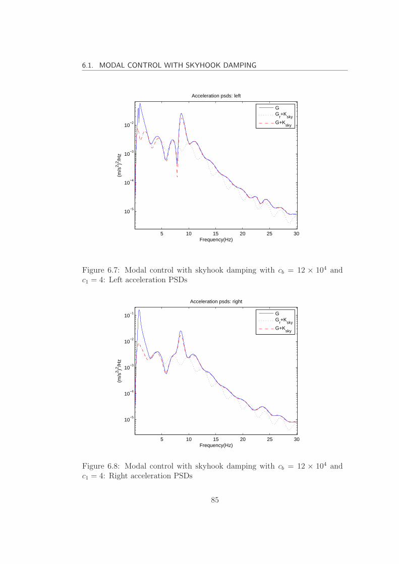
6.1. MODAL CONTROL WITH SKYHOOK DAMPING
5 10 15 20 25 30
10−5
10−4
10−3
10−2
Acceleration psds: left
Frequency(Hz)
(m/s
2 )2 /Hz
GG
r+K
sky
G+Ksky
Figure 6.7: Modal control with skyhook damping with cb = 12 × 104 andc1 = 4: Left acceleration PSDs
5 10 15 20 25 30
10−5
10−4
10−3
10−2
10−1
Acceleration psds: right
Frequency(Hz)
(m/s
2 )2 /Hz
GG
r+K
sky
G+Ksky
Figure 6.8: Modal control with skyhook damping with cb = 12 × 104 andc1 = 4: Right acceleration PSDs
85
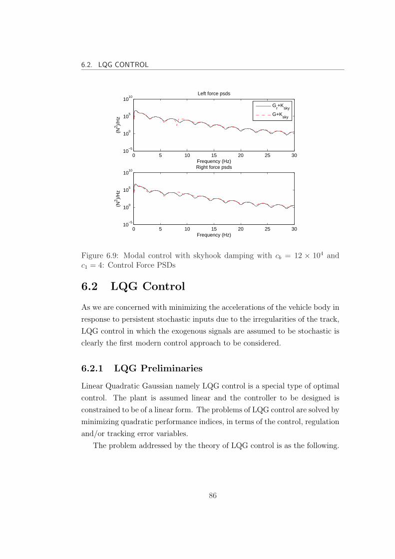
6.2. LQG CONTROL
0 5 10 15 20 25 3010
−5
100
105
1010
Frequency (Hz)
(N2 )/
Hz
Left force psds
0 5 10 15 20 25 3010
−5
100
105
1010
Frequency (Hz)
(N2 )/
Hz
Right force psds
Gr+K
sky
G+Ksky
Figure 6.9: Modal control with skyhook damping with cb = 12 × 104 andc1 = 4: Control Force PSDs
6.2 LQG Control
As we are concerned with minimizing the accelerations of the vehicle body in
response to persistent stochastic inputs due to the irregularities of the track,
LQG control in which the exogenous signals are assumed to be stochastic is
clearly the first modern control approach to be considered.
6.2.1 LQG Preliminaries
Linear Quadratic Gaussian namely LQG control is a special type of optimal
control. The plant is assumed linear and the controller to be designed is
constrained to be of a linear form. The problems of LQG control are solved by
minimizing quadratic performance indices, in terms of the control, regulation
and/or tracking error variables.
The problem addressed by the theory of LQG control is as the following.
86
6.2. LQG CONTROL
Given a plant model in state-space form,
x = Ax + Bu + Gwd (6.14)
y = Cx + Du + Hwd + wn (6.15)
where wd and wn are vectors of the disturbance (process noise) and mea-
surement noise respectively, which are usually assumed to be white noises,
namely zero-mean Gaussian stochastic processes which are uncorrelated in
time, having the covariance,
EwdwdT = W ≥ 0, EwnwT
n = V ≥ 0 (6.16)
Here it is assumed that wd and wn are uncorrelated with each other
EwdwnT = 0 (6.17)
u is the vector of control signals, y is the vector of measured outputs which
is corrupted by wn. The problem is to devise a feedback-control law which
minimizes the cost
J = limT→∞
E
∫ T
0
[z(t)TQz(t) + uT (t)Ru(t)]
(6.18)
where z(t) could be the state vector x(t) or some linear combination of the
states
z(t) = Mx(t) (6.19)
Q and R are weighting matrices, which are symmetrical and definite
Q = QT ≥ 0, R = RT > 0 (6.20)
The LQG problem includes the optimal estimation problem and linear
quadratic control problem. The solution to the LQG problem is based on the
separation principle, illustrated in Figure 6.10. Firstly determine the optimal
control for a deterministic linear quadratic regulator (LQR) problem. The
87
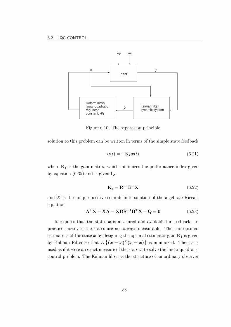
6.2. LQG CONTROL
Plant
Deterministiclinear quadraticregulatorconstant, -Kr
Kalman filter dynamic systemx
u y
wd wn
Figure 6.10: The separation principle
solution to this problem can be written in terms of the simple state feedback
u(t) = −Krx(t) (6.21)
where Kr is the gain matrix, which minimizes the performance index given
by equation (6.35) and is given by
Kr = R−1BTX (6.22)
and X is the unique positive semi-definite solution of the algebraic Riccati
equation
ATX + XA−XBR−1BTX + Q = 0 (6.23)
It requires that the states x is measured and available for feedback. In
practice, however, the states are not always measurable. Then an optimal
estimate x of the state x by designing the optimal estimator gain Kf is given
by Kalman Filter so that E(x − x)T (x − x)
is minimized. Then x is
used as if it were an exact measure of the state x to solve the linear quadratic
control problem. The Kalman filter as the structure of an ordinary observer
88
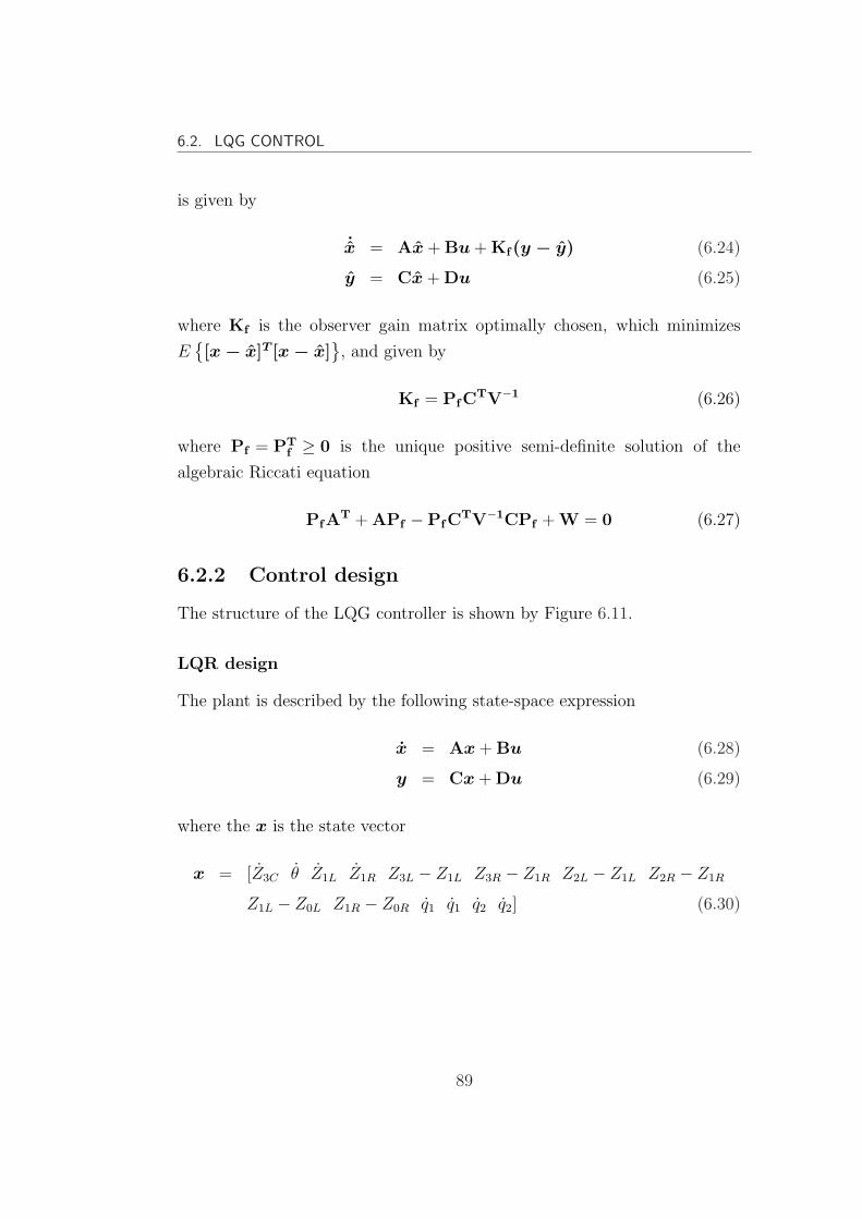
6.2. LQG CONTROL
is given by
˙x = Ax + Bu + Kf(y − y) (6.24)
y = Cx + Du (6.25)
where Kf is the observer gain matrix optimally chosen, which minimizes
E[x − x]T [x − x]
, and given by
Kf = PfCTV−1 (6.26)
where Pf = PTf ≥ 0 is the unique positive semi-definite solution of the
algebraic Riccati equation
PfAT + APf −PfC
TV−1CPf + W = 0 (6.27)
6.2.2 Control design
The structure of the LQG controller is shown by Figure 6.11.
LQR design
The plant is described by the following state-space expression
x = Ax + Bu (6.28)
y = Cx + Du (6.29)
where the x is the state vector
x = [Z3C θ Z1L Z1R Z3L − Z1L Z3R − Z1R Z2L − Z1L Z2R − Z1R
Z1L − Z0L Z1R − Z0R q1 q1 q2 q2] (6.30)
89
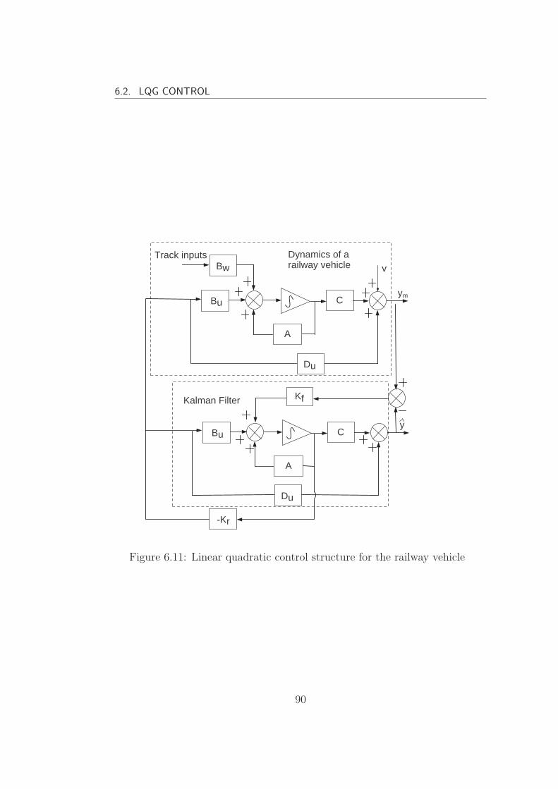
6.2. LQG CONTROL
Bu
A
C
Du
Bu
A
C
Du
Kf
-Kr
BwTrack inputs
ym
y
vDynamics of arailway vehicle
Kalman Filter
Figure 6.11: Linear quadratic control structure for the railway vehicle
90
6.2. LQG CONTROL
u = [UL UR], and the matrices A and B have been given in Chapter 4. If a
rigid model is used for control design, the state vector is given by
x = [Z3C θ Z1L Z1R Z3L − Z1L Z3R − Z1R Z2L − Z1L Z2R − Z1R
Z1L − Z0L Z1R − Z0R] (6.31)
and the matrices A and B change accordingly.
The regulated output vector is chosen as three accelerations of the vehicle
body and two suspension deflections
y = [ZxLZxC
ZxRZ3L − Z1L Z3R − Z1R] (6.32)
The control objective is to minimize the accelerations while maintaining
the suspension deflection at an acceptable level and keeping the control inputs
small. Output weighting is used instead of state weighting because not all the
regulated variables (e.g the accelerations of the vehicle body) can be found
in the state variables.
y(t)TQyy(t) = (Cx(t) + Du(t))TQy(Cx(t) + Du(t))
= x(t)TCTQyCx(t) + 2x(t)TCTQyDu(t) + u(t)TDTDu(t)
(6.33)
where and Qy is the output weighting matrix written as
Qy =
q1 0 0 0 0
0 q1 0 0 0
0 0 q1 0 0
0 0 0 q2 0
0 0 0 0 q2
(6.34)
where q1 is the weight for the accelerations and q2 is the weight for suspension
91
6.2. LQG CONTROL
deflections. The quadratic cost function is rewritten into
J = limT→∞
E
∫ T
0
[y(t)TQyy(t)]
= limT→∞
E
∫ T
0
[x(t)TQx(t) + uT (t)Ru(t) + 2x(t)TNu(t)]
(6.35)
Hence Q = CTQyC, R = DTD and N = CTQyD. With the selection of
output weight of Qy, the values for weights of Q, R and N are determined.
The selection of quadratic weights is difficult and mainly depends on the
experience of the designer. Here elements in Qy are initially chosen to be
square of the inverse of the expected values, 1(expected value)2
, then they are
tuned based on the physical constraints (e.g. deflection≤ 12mm , control
force≤ 4kN). There is a trade-off between the accelerations and suspension
deflections. Increasing q1 leads to smaller accelerations, larger deflections and
bigger force inputs and vice versa. Increasing q2 leads to smaller deflections,
larger accelerations and smaller force inputs and vise versa. The optimal
state-feedback gain K is given by equation (6.21). In MATLAB, the following
command is used
[K,S,e]=lqr(A,B,Q,R,N)
Kalman filter
Kalman-Bucy filter, the continuous time version of the Kalman filter, is
designed to estimate the states of the system. Recall the model of the plant
x = Ax + Buu + Bww (6.36)
ym = Cmx + Dmu + Dww + v (6.37)
The system is subject to random track disturbances w = [Z0L Z0R]. The
measurements feeding to the estimator are chosen as the three accelerations
of the vehicle body
ym = [ZxLZxC
ZxR] (6.38)
92
6.2. LQG CONTROL
ym is corrupted by the sensor noises v
For selection of W and V, they are considered more as representations
of aspects of the real problem than as tuning parameters, which are to be
adjusted until a satisfactory design is obtained. W is given by the track
variance and the measurement noise is normally assumed to have an RMS
value of one percent of the maximum acceleration. Based on the above
principles, W and V are chosen as
W =
[5.4283× 10⁻⁴ 0
0 5.4283× 10⁻⁴
](6.39)
V =
(0.01× 0.365)2 0 0
0 (0.01× 0.365)2 0
0 0 (0.01× 0.365)2
(6.40)
It is very important to choose the correct track variance for the process noise
and the correct level of sensor noise because they will affect the ride quality of
the vehicle(Foo and Goodall [2000]). Then the best Kf is given by equation
(6.26). In MATLAB Kf and the LQG controller are found with the following
commands
sys_kf=ss(Ar,[Br Bw],Cm,[Dm Dw]);
[Kf,L,P]=kalman(sys_kf,W,V);
K_lqg=lqgreg(Kf,Kr);
6.2.3 Results and discussion
The LQG controller has been designed using the rigid model (Gr) and the
flexible model (G), and the resulting controllers are denoted by KrLQG and
KLQG respectively.
Results with controller KrLQG
Controller KrLQG is designed with the rigid model Gr of the railway vehicle.
Results tabulated in Table 6.2 are RMS acceleration levels in %g , RMS values
of suspension deflections and RMS values of control forces. Step responses of
93

6.2. LQG CONTROL
Table 6.2: RMS results: LQG control design with rigid model with q1 =1/(0.1)2 and q2 = 1/(0.012)2
Sys.Vertical Acc.(%g) Susp. Def.(mm) Act. Force(kN)
Center Left Right Left Right Left RightKrLQG + Gr 0.35 0.51 0.53 10.27 10.69 3.82 3.97KrLQG + G 0.46 0.53 0.57 10.27 10.70 3.82 3.97
the accelerations are shown in Figure 6.12. High frequency oscillations appear
in the step responses when the controller is simulated with the flexible model.
Figure 6.13, 6.14 and 6.15 give power spectral densities (PSDs) for the
centre (xC), left (xL) and right (xR) accelerations of the railway vehicle in
response to random track disturbances.
LQG controller gives significantly bigger improvement in ride quality than
classical control approach with skyhook damping and the forces are generally
increased with LQG controller. However, comparing the results, it also shows
that the flexibility of the vehicle body worsens the ride quality when the
controller is designed without considering the effect of the flexible modes,
even though the accelerations of the rigid motions of the vehicle body are
well reduced and the RMS levels of the accelerations are considerably small.
The plots in Figure 6.16 shows that the PSDs of the control forces of
system (Gr + KrLQG) and system (G + KrLQG) are almost the same.
Results with controller KLQG
Controller KLQG is designed with the flexible model, G, of the railway vehicle.
Results tabulated in Table 6.3 are RMS acceleration levels in %g , RMS values
of suspension deflections and RMS values of control forces with different
values for weight q1. The RMS results show excellent improvement in ride
quality.
Step responses of the accelerations are shown in Figure 6.17. It shows
that the high frequency vibrations caused by the flexibility of the vehicle
body have been suppressed.
Figure 6.18, 6.19 ,6.20 and 6.21 give PSDs for the centre (xC), left (xL)
and right (xR) accelerations and PSDs for the suspension control forces of
94
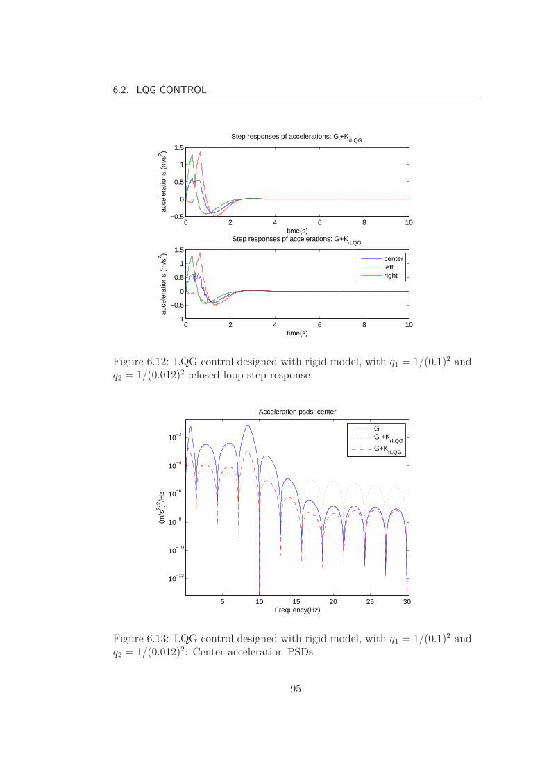
6.2. LQG CONTROL
0 2 4 6 8 10−0.5
0
0.5
1
1.5
time(s)
acce
lera
tions
(m
/s2 )
Step responses pf accelerations: Gr+K
rLQG
0 2 4 6 8 10−1
−0.5
0
0.5
1
1.5
time(s)
acce
lera
tions
(m
/s2 )
Step responses pf accelerations: G+KrLQG
centerleftright
Figure 6.12: LQG control designed with rigid model, with q1 = 1/(0.1)2 andq2 = 1/(0.012)2 :closed-loop step response
5 10 15 20 25 30
10−12
10−10
10−8
10−6
10−4
10−2
Acceleration psds: center
Frequency(Hz)
(m/s
2 )2 /Hz
GG
r+K
rLQG
G+KrLQG
Figure 6.13: LQG control designed with rigid model, with q1 = 1/(0.1)2 andq2 = 1/(0.012)2: Center acceleration PSDs
95
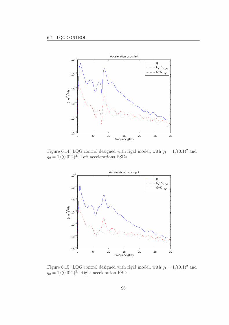
6.2. LQG CONTROL
0 5 10 15 20 25 3010
−6
10−5
10−4
10−3
10−2
10−1
Acceleration psds: left
Frequency(Hz)
(m/s
2 )2 /Hz
GG
r+K
rLQG
G+KrLQG
Figure 6.14: LQG control designed with rigid model, with q1 = 1/(0.1)2 andq2 = 1/(0.012)2: Left accelerations PSDs
0 5 10 15 20 25 3010
−6
10−5
10−4
10−3
10−2
10−1
100
Acceleration psds: right
Frequency(Hz)
(m/s
2 )2 /Hz
GG
r+K
rLQG
G+KrLQG
Figure 6.15: LQG control designed with rigid model, with q1 = 1/(0.1)2 andq2 = 1/(0.012)2: Right acceleration PSDs
96

6.2. LQG CONTROL
0 5 10 15 20 25 3010
2
104
106
108
Frequency(Hz)
(N2 )/
Hz
left force psds
0 5 10 15 20 25 3010
2
104
106
108
Frequency(Hz)
(N2 )/
Hz
right force psds
Gr+K
rLQG
G+KrLQG
Figure 6.16: LQG control designed with rigid model, with q1 = 1/(0.1)2 andq2 = 1/(0.012)2:Control force PSDs
Table 6.3: RMS results: LQG control designed with flexible model withq2 = 1/(0.012)2
Para. Vertical Acc.(%g) Susp. Def.(mm) Act. Force(kN)q1 Center Left Right Left Right Left Right
1/(0.20)2 0.53 0.81 0.86 8.78 9.20 3.16 3.331/(0.15)2 0.45 0.66 0.71 9.40 9.84 3.46 3.621/(0.10)2 0.36 0.50 0.54 10.33 10.79 3.87 4.02
0 2 4 6 8 10−0.5
0
0.5
1
1.5
Step responses of accelerations: G+KLQG
time(s)
acce
lera
tions
(m
/s2 )
centerleftright
Figure 6.17: LQG control designed with flexible model, with q1 = 1/(0.1)2
and q2 = 1/(0.012)2 :closed-loop step response
97
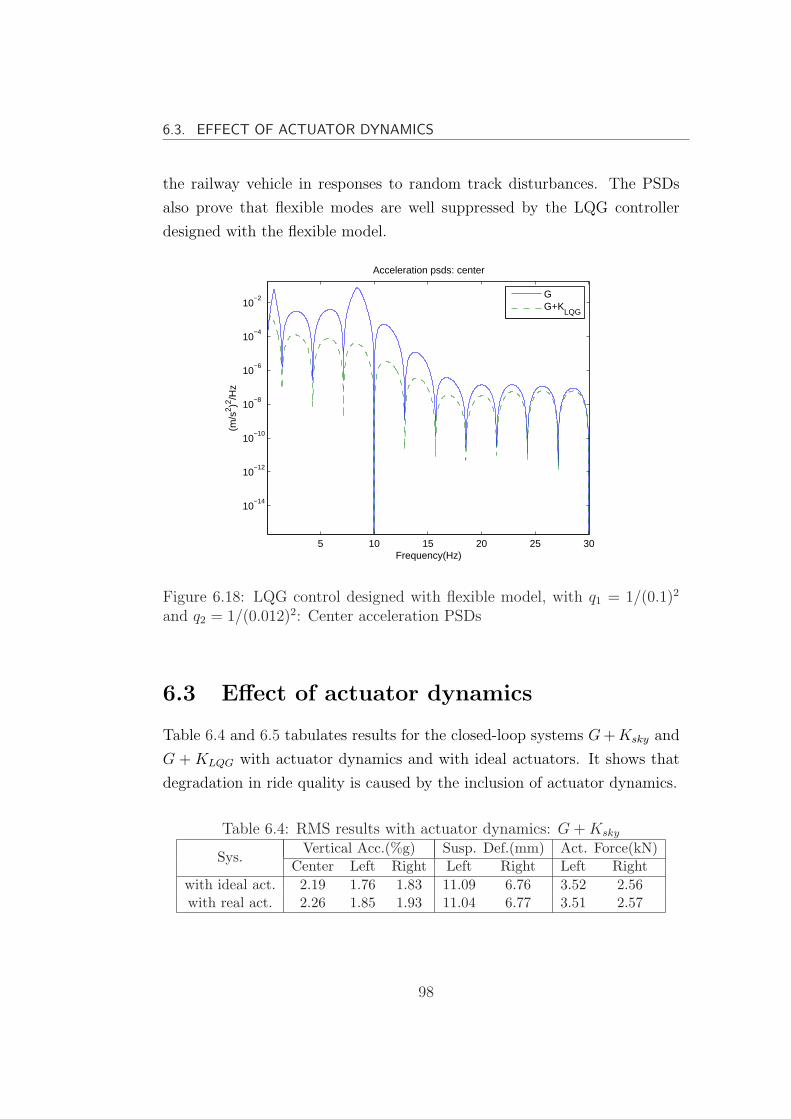
6.3. EFFECT OF ACTUATOR DYNAMICS
the railway vehicle in responses to random track disturbances. The PSDs
also prove that flexible modes are well suppressed by the LQG controller
designed with the flexible model.
5 10 15 20 25 30
10−14
10−12
10−10
10−8
10−6
10−4
10−2
Acceleration psds: center
Frequency(Hz)
(m/s
2 )2 /Hz
GG+K
LQG
Figure 6.18: LQG control designed with flexible model, with q1 = 1/(0.1)2
and q2 = 1/(0.012)2: Center acceleration PSDs
6.3 Effect of actuator dynamics
Table 6.4 and 6.5 tabulates results for the closed-loop systems G + Ksky and
G + KLQG with actuator dynamics and with ideal actuators. It shows that
degradation in ride quality is caused by the inclusion of actuator dynamics.
Table 6.4: RMS results with actuator dynamics: G + Ksky
Sys.Vertical Acc.(%g) Susp. Def.(mm) Act. Force(kN)
Center Left Right Left Right Left Rightwith ideal act. 2.19 1.76 1.83 11.09 6.76 3.52 2.56with real act. 2.26 1.85 1.93 11.04 6.77 3.51 2.57
98

6.3. EFFECT OF ACTUATOR DYNAMICS
0 5 10 15 20 25 3010
−6
10−5
10−4
10−3
10−2
10−1
Acceleration psds: left
Frequency(Hz)
(m/s
2 )2 /Hz
GG+K
LQG
Figure 6.19: LQG control designed with flexible model, with q1 = 1/(0.1)2
and q2 = 1/(0.012)2: Left accelerations PSDs
0 5 10 15 20 25 3010
−6
10−5
10−4
10−3
10−2
10−1
100
Acceleration psds: right
Frequency(Hz)
(m/s
2 )2 /Hz
GG+K
LQG
Figure 6.20: LQG control designed with flexible model, with q1 = 1/(0.1)2
and q2 = 1/(0.012)2: Right acceleration PSDs
99
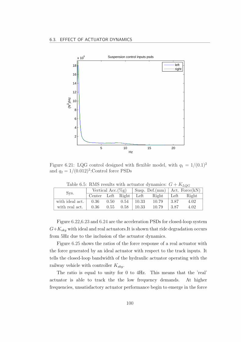
6.3. EFFECT OF ACTUATOR DYNAMICS
5 10 15 20
2
4
6
8
10
12
14
16
18
x 106
Hz
(N2 )/
Hz
Suspension control inputs psds
leftright
Figure 6.21: LQG control designed with flexible model, with q1 = 1/(0.1)2
and q2 = 1/(0.012)2:Control force PSDs
Table 6.5: RMS results with actuator dynamics: G + KLQG
Sys.Vertical Acc.(%g) Susp. Def.(mm) Act. Force(kN)
Center Left Right Left Right Left Rightwith ideal act. 0.36 0.50 0.54 10.33 10.79 3.87 4.02with real act. 0.36 0.55 0.58 10.33 10.79 3.87 4.02
Figure 6.22,6.23 and 6.24 are the acceleration PSDs for closed-loop system
G+Ksky with ideal and real actuators.It is shown that ride degradation occurs
from 5Hz due to the inclusion of the actuator dynamics.
Figure 6.25 shows the ratios of the force response of a real actuator with
the force generated by an ideal actuator with respect to the track inputs. It
tells the closed-loop bandwidth of the hydraulic actuator operating with the
railway vehicle with controller Ksky.
The ratio is equal to unity for 0 to 4Hz. This means that the ’real’
actuator is able to track the the low frequency demands. At higher
frequencies, unsatisfactory actuator performance begin to emerge in the force
100
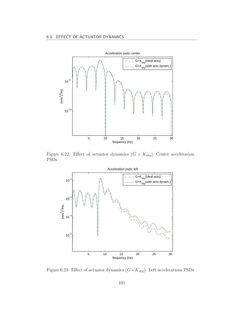
6.3. EFFECT OF ACTUATOR DYNAMICS
5 10 15 20 25 30
10−10
10−5
Acceleration psds: center
frequency (Hz)
(m/s
2 )2 /Hz
G+K
sky(ideal actu)
G+Ksky
(with actu dynam.)
Figure 6.22: Effect of actuator dynamics (G + Ksky) :Center accelerationPSDs
5 10 15 20 25 30
10−5
10−4
10−3
10−2
Acceleration psds: left
frequency (Hz)
(m/s
2 )2 /Hz
G+K
sky(ideal actu)
G+Ksky
(with actu dynam.)
Figure 6.23: Effect of actuator dynamics (G+Ksky): Left accelerations PSDs
101
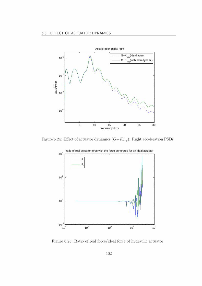
6.3. EFFECT OF ACTUATOR DYNAMICS
5 10 15 20 25 30
10−5
10−4
10−3
10−2
Acceleration psds: right
frequency (Hz)
(m/s
2 )2 /Hz
G+K
sky(ideal actu)
G+Ksky
(with actu dynam.)
Figure 6.24: Effect of actuator dynamics (G+Ksky): Right acceleration PSDs
10−2
10−1
100
101
102
10−1
100
101
102
ratio of real actuator force with the force generated for an ideal actuator
Ul
Ur
Figure 6.25: Ratio of real force/ideal force of hydraulic actuator
102
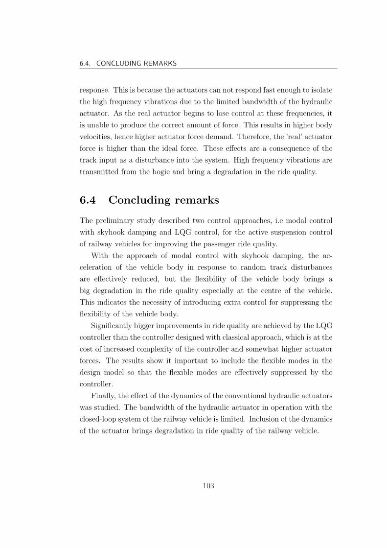
6.4. CONCLUDING REMARKS
response. This is because the actuators can not respond fast enough to isolate
the high frequency vibrations due to the limited bandwidth of the hydraulic
actuator. As the real actuator begins to lose control at these frequencies, it
is unable to produce the correct amount of force. This results in higher body
velocities, hence higher actuator force demand. Therefore, the ’real’ actuator
force is higher than the ideal force. These effects are a consequence of the
track input as a disturbance into the system. High frequency vibrations are
transmitted from the bogie and bring a degradation in the ride quality.
6.4 Concluding remarks
The preliminary study described two control approaches, i.e modal control
with skyhook damping and LQG control, for the active suspension control
of railway vehicles for improving the passenger ride quality.
With the approach of modal control with skyhook damping, the ac-
celeration of the vehicle body in response to random track disturbances
are effectively reduced, but the flexibility of the vehicle body brings a
big degradation in the ride quality especially at the centre of the vehicle.
This indicates the necessity of introducing extra control for suppressing the
flexibility of the vehicle body.
Significantly bigger improvements in ride quality are achieved by the LQG
controller than the controller designed with classical approach, which is at the
cost of increased complexity of the controller and somewhat higher actuator
forces. The results show it important to include the flexible modes in the
design model so that the flexible modes are effectively suppressed by the
controller.
Finally, the effect of the dynamics of the conventional hydraulic actuators
was studied. The bandwidth of the hydraulic actuator in operation with the
closed-loop system of the railway vehicle is limited. Inclusion of the dynamics
of the actuator brings degradation in ride quality of the railway vehicle.
103
Chapter 7
Control Design I: Decentralized
Control
This chapter describes the decentralized control strategy for vibration control
of the railway vehicle considering the flexible modes of the vehicle body with
the combined conventional active suspension control and active structural
damping. It includes the controller design for active damping of the flexible
structure of the vehicle with piezoelectric stack actuators and piezoelectric
patch sensors, and the controller design for the secondary active suspension
control. The two sub controllers are designed independently with decoupled
parts of the overall model. In contrast, centralized controller designed with
the full model will be considered in chapter 8.
Two combinations of control methods will be considered in this chapter:
1) modal control with skyhook damping for suspension control and LQG
control for structural damping. 2) Two individual LQG controllers for
structural damping and suspension control respectively.
7.1 Introduction of active structural damp-
ing
For active structural damping, piezoelectric actuators and sensors are
integrated onto the flexible structure of the railway vehicle body. The signals
104
7.2. STRUCTURE OF DECENTRALIZED CONTROL
from the sensors are fedback to the controller, and the control signal is
produced to drive the actuator to produce the necessary moments/force
acting on the flexible structure. The structure integrated with actuators,
sensors and control is viewed as a smart structure.
Structural damping is necessary for flexible-bodied railway vehicles,
although active suspension control is able to improve the ride quality by
suppressing both the rigid modes and flexible modes with careful control
design. According to the state-space representation of the system model
given by equation 4.59, the flexible motion and the rigid motion are coupled
(the coupling is discussed in detail in section 4.5). Briefly speaking, coupling
is introduced by actuation (e.g. forces from the secondary suspension) that
affects both the flexible modes and rigid modes and sensing (e.g. by the
conventional accelerometers) that measures both the flexible modes and
rigid modes. However, the performance of active suspension control for
suppressing the flexible modes using the actuators alone is limited due to
several reasons
The positions of the suspension control xL and xR are near the node
points of the 1st vertical bending mode, which is the critical flexible
mode for ride quality under consideration.
The limited bandwidth of the conventional actuators (e.g hydraulic
actuator) for suspension control.
The real vehicle body structure is much more complex than a simple
beam. The elastic modes include vertical, horizontal bending mode,
torsional and diagonal distortion mode (Popprath et al. [July 2006]).
7.2 Structure of decentralized control
The structure of a decentralized control for a regulation problem is shown in
Figure 7.1 (Skogestad and Postletwaite [2005]). G(s) is the plant model,
which includes the rigid modes and the first two flexible vertical modes
of the vehicle body. G(s) is also called the full model in the following
105
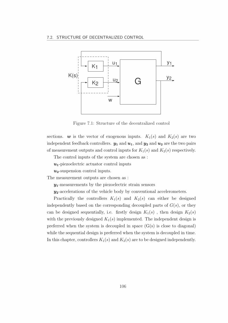
7.2. STRUCTURE OF DECENTRALIZED CONTROL
G
K1
K2
y1
y2K(s)
u1
u2
w
Figure 7.1: Structure of the decentralized control
sections. w is the vector of exogenous inputs. K1(s) and K2(s) are two
independent feedback controllers. y1 and u1, and y2 and u2 are the two pairs
of measurement outputs and control inputs for K1(s) and K2(s) respectively.
The control inputs of the system are chosen as :
u1-piezoelectric actuator control inputs
u2-suspension control inputs.
The measurement outputs are chosen as :
y1-measurements by the piezoelectric strain sensors
y2-accelerations of the vehicle body by conventional accelerometers.
Practically the controllers K1(s) and K2(s) can either be designed
independently based on the corresponding decoupled parts of G(s), or they
can be designed sequentially, i.e. firstly design K1(s) , then design K2(s)
with the previously designed K1(s) implemented. The independent design is
preferred when the system is decoupled in space (G(s) is close to diagonal)
while the sequential design is preferred when the system is decoupled in time.
In this chapter, controllers K1(s) and K2(s) are to be designed independently.
106
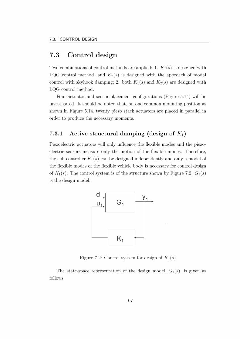
7.3. CONTROL DESIGN
7.3 Control design
Two combinations of control methods are applied: 1. K1(s) is designed with
LQG control method, and K2(s) is designed with the approach of modal
control with skyhook damping; 2. both K1(s) and K2(s) are designed with
LQG control method.
Four actuator and sensor placement configurations (Figure 5.14) will be
investigated. It should be noted that, on one common mounting position as
shown in Figure 5.14, twenty piezo stack actuators are placed in parallel in
order to produce the necessary moments.
7.3.1 Active structural damping (design of K1)
Piezoelectric actuators will only influence the flexible modes and the piezo-
electric sensors measure only the motion of the flexible modes. Therefore,
the sub-controller K1(s) can be designed independently and only a model of
the flexible modes of the flexible vehicle body is necessary for control design
of K1(s). The control system is of the structure shown by Figure 7.2. G1(s)
is the design model.
G1
K1
d
u1
y1
Figure 7.2: Control system for design of K1(s)
The state-space representation of the design model, G1(s), is given as
follows
107

7.3. CONTROL DESIGN
xf = Afxf + Bf1u1 + Bf2d (7.1)
y1 = Cvxf (7.2)
yf = C2xf + D12u1 + D22d (7.3)
where Af is the (n×n) system matrix, where n is the number of states. Bf1
is the (n × 2) disturbance input matrix, Bf2 is the (n × np) input matrix,
Cv is the(mp × n) measurement output matrix. u1 is the (np × 1) vector
of control signals(from the piezoelectric actuators), d is the (2 × 1) vector
of disturbances (from secondary suspensions), y1 is the (mp × 1) vector of
measured variables (by piezoelectric sensors),yf is the vector of controlled
variables.
Configuration 1 For configuration 1, The first two flexible modal
coordinates and the first derivative of the modal coordinates are included
as the states of the state-space model of G1.
xf =[
q1 q1 q2 q2
]T
(7.4)
The system matrix Af , the voltage input matrix Bf1, the disturbance input
matrix Bf2 and the measurement output matrix Cv are in the following form:
Af =
−2ζ1ω1 −ω21 0
1 0 0 0
0 0 −2ζ2ω2 −ω22
0 0 1 0
(7.5)
Bf1 =Ka
Mv
Ψa11 Ψa12 Ψa13
0 0 0
Ψa21 Ψa22 Ψa23
0 0 0
(7.6)
108
7.3. CONTROL DESIGN
Bf2 =
φ1(xL)Mv
φ1(xR)Mv
0 0φ2(xL)
Mv
φ2(xR)Mv
0 0
(7.7)
Cv =Ks
Cp
0 Ψs1(xC) 0 Ψs2(xC)
0 Ψs1(xL) 0 Ψs2(xL)
0 Ψs1(xR) 0 Ψs2(xR)
(7.8)
Configurations 2 For configurations 2,3 and 4, piezoelectric actuators
and sensors are placed at the centre of the vehicle for controlling the first
flexible modes. The design model G1 contains only the first flexible mode.
The state vector is written as
xf =[
q1 q1
]T
(7.9)
The system matrix and the disturbance input matrix are in the following
form:
Af =
[−2ζ1w1 −w2
1
1 0
](7.10)
Bf2 =
[φ1(xL)
Mv
φ1(xR)Mv
0 0
](7.11)
The voltage input matrix and the measurement output matrix are as follows
Bf1 =Ka
Mv
[Ψa11
0
](7.12)
Cv =Ks
Cp
[0 Ψs11
](7.13)
Configuration 3 There are three actuators and one sensor placed at the
centre of the beam (railway vehicle body). For the state-space representation
of the design model of G1, the state vector xf , the system matrix Af , the
disturbance input matrix Bf2 and the measurement output matrix Cv are
in the same form as given for configuration 2. The input matrix Bf1 is as
109
7.3. CONTROL DESIGN
follows
Bf1 =Ka
Mv
[Ψa11 Ψa12 Ψa13
0 0 0
](7.14)
Configuration 4 There are three actuators and three sensor placed at
the centre of the beam (railway vehicle body). For the state-space model
of G1(s), the state vector xf , system matrix Af and the disturbance input
matrix Bf2 are in the same form as given for configuration 2. The input
matrix Bf1 is in the same form as given for configuration 3. The measurement
output matrix is as follows
Cv =Ks
Cp
0 Ψs11
0 Ψs12
0 Ψs13
(7.15)
Control design
The aim of the control design is minimizing the accelerations of flexible
motion at the chosen performance positions, thereby improving the passenger
ride quality of the vehicle. In other words, it is aimed to increase the
damping ratio of the flexible modes. Though the approach of pole placement
is straightforward to increase the damping ratios of the flexible modes, it
is hard to control the control inputs. Therefore, LQG control method is
adopted to design K1(s). Preliminaries on LQG control have been given in
section 6.2.1.
The performance positions are chosen as the centre of the vehicle, xC ,
position of left suspension, xL, and position of the right suspension, xL.
Accelerations of the flexible modes are chosen as the controlled variables.
For configuration 1 the vector of controlled variables is given by
yf =
φ1(xC)q1 + φ2(xC)q2
φ1(xL)q1 + φ2(xL)q2
φ1(xR)q1 + φ2(xR)q2
(7.16)
110
7.3. CONTROL DESIGN
and for configuration 2,3,4, the vector of controlled variables is given by
yf = φ1(xC)q1 (7.17)
The cost function is given as the following
J = limT→∞
E
∫ T
0
[yf (t)TQyyf (t) + u(t)TR0u(t)]
(7.18)
where R0 is the input weighting matrix and its elements are fixed at 1. Qy
is the output weighting matrix and are written in the form as follows for the
four configurations:
for configuration 1
Qy = diag1/(qy1)2, 1/(qy2)
2, 1/(qy3)2 (7.19)
and for configuration 2,3,4
Qy = 1/(qy1)2 (7.20)
where q1, q2 and q3 are usually initially chosen as the expected values
of the controlled variables and further tuned accordingly to achieve the
best performance while maintaining the input voltages of the piezoelectric
actuators within their limits.
Kalman filter is designed to estimate the states of the system. The system
is subject to disturbances from the secondary suspensions d. The variance
of the disturbance obtained from the simulation results of the passive system
of the railway system
W = diag2.5× 10−4, 2.5× 10⁻⁴ (7.21)
The piezoelectric sensor patches measure the strain in the beam by feeding
111
7.3. CONTROL DESIGN
back voltage signals. For configurations 1 and 4,
y1 =
vs1
vs2
vs3
(7.22)
and for configurations 2 and 3,
y1 =[
vs1
](7.23)
The measurement noise is assumed to have an RMS value of one percent of
the maximum value measured by the sensors. However the variance of the
measurement noise is further tuned until the estimator can provide a good
performance for the system. For configurations 1 and 4
V = diag1× 10−18, 1× 10⁻¹⁸, 1× 10⁻¹⁸ (7.24)
and for configurations 2 and 3
V = diag1× 10−18 (7.25)
Very small value have been chosen for V, which implies that the sensors are
almost perfect. This will cause potential robustness problems in practice.
Results and discussion
In the following, it is going to examine the closed-loop of the railway vehicle
system G(s) with the LQG controller K1(s).
The eigenvalues and modal damping ratios ξi for the controlled flexible
modes are tabulated in Table 7.1. Damping ratio of the first two flexible
modes of the passive system are ξ1 = 0.05 and ξ2 = 0.051. It shows that the
damping ratios have been effectively increased by the controller.
Table 7.2 tabulates the RMS acceleration levels at the centre (xC), left
(xL) and right (xR) of the vehicle, the RMS suspension deflection values at
left (xL) and right (xR) of the vehicle, and the RMS voltage input levels
112
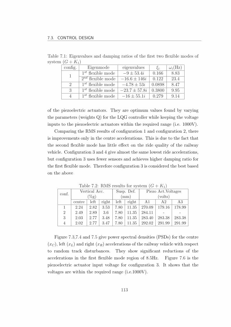
7.3. CONTROL DESIGN
Table 7.1: Eigenvalues and damping ratios of the first two flexible modes ofsystem (G + K1)
config. Eigenmode eigenvalues ξi ωi(Hz)
11st flexible mode −9± 53.4i 0.166 8.832nd flexible mode −16.6± 146i 0.122 23.4
2 1st flexible mode −4.78± 53i 0.0898 8.473 1st flexible mode −23.7± 57.8i 0.3800 9.954 1st flexible mode −16± 55.1i 0.279 9.14
of the piezoelectric actuators. They are optimum values found by varying
the parameters (weights Q) for the LQG controller while keeping the voltage
inputs to the piezoelectric actuators within the required range (i.e. 1000V).
Comparing the RMS results of configuration 1 and configuration 2, there
is improvements only in the centre accelerations. This is due to the fact that
the second flexible mode has little effect on the ride quality of the railway
vehicle. Configuration 3 and 4 give almost the same lowest ride accelerations,
but configuration 3 uses fewer sensors and achieves higher damping ratio for
the first flexible mode. Therefore configuration 3 is considered the best based
on the above
Table 7.2: RMS results for system (G + K1)
conf.Vertical Acc. Susp. Def. Piezo Act.Voltages
(%g) (mm) (volts)centre left right left right A1 A2 A3
1 2.24 2.82 3.53 7.80 11.35 270.09 179.16 178.992 2.49 2.89 3.6 7.80 11.35 284.11 - -3 2.03 2.77 3.48 7.80 11.35 283.40 283.38 283.384 2.02 2.77 3.47 7.80 11.35 292.02 291.99 291.99
Figure 7.3,7.4 and 7.5 give power spectral densities (PSDs) for the centre
(xC), left (xL) and right (xR) accelerations of the railway vehicle with respect
to random track disturbances. They show significant reductions of the
accelerations in the first flexible mode region of 8.5Hz. Figure 7.6 is the
piezoelectric actuator input voltage for configuration 3. It shows that the
voltages are within the required range (i.e.1000V).
113
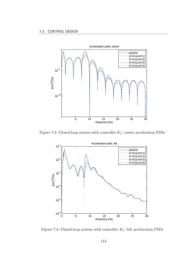
7.3. CONTROL DESIGN
5 10 15 20 25 30
10−10
10−5
Acceleration psds: centre
frequency (Hz)
(m/s
2 )2 /Hz
passiveG+K1(conf.1)G+K1(conf.2)G+K1(conf.3)G+K1(conf.4)
Figure 7.3: Closed-loop system with controller K1: centre acceleration PSDs
0 5 10 15 20 25 3010
−6
10−5
10−4
10−3
10−2
10−1
Acceleration psds: left
frequency (Hz)
(m/s
2 )2 /Hz
passiveG+K1(conf.1)G+K1(conf.2)G+K1(conf.3)G+K1(conf.4)
Figure 7.4: Closed-loop system with controller K1: left acceleration PSDs
114
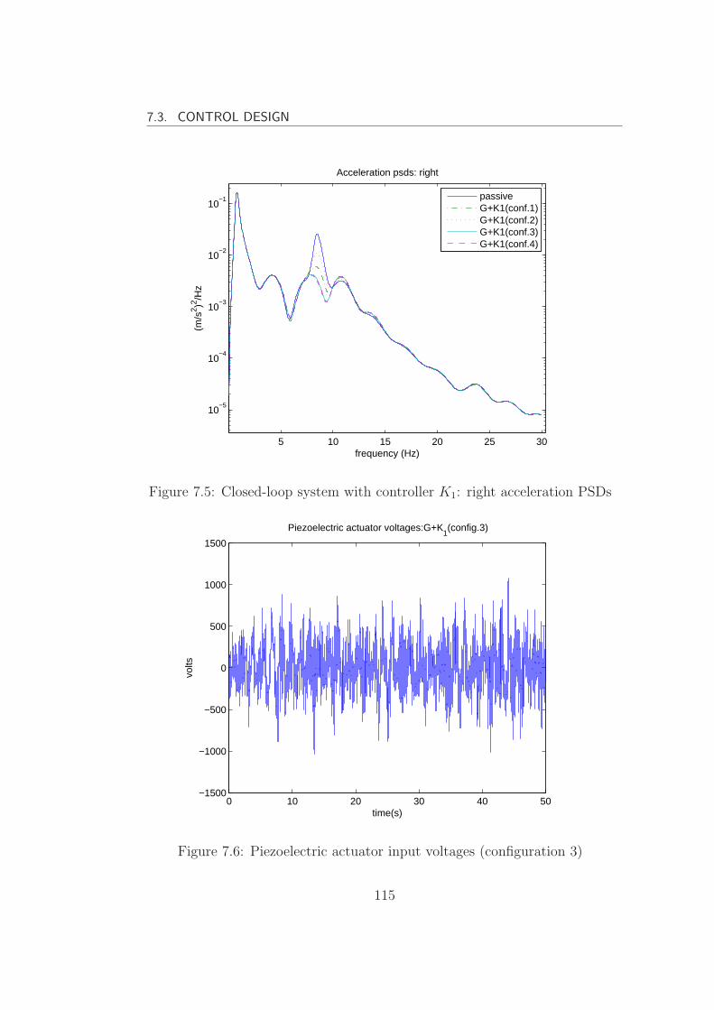
7.3. CONTROL DESIGN
5 10 15 20 25 30
10−5
10−4
10−3
10−2
10−1
Acceleration psds: right
frequency (Hz)
(m/s
2 )2 /Hz
passiveG+K1(conf.1)G+K1(conf.2)G+K1(conf.3)G+K1(conf.4)
Figure 7.5: Closed-loop system with controller K1: right acceleration PSDs
0 10 20 30 40 50−1500
−1000
−500
0
500
1000
1500
Piezoelectric actuator voltages:G+K1(config.3)
time(s)
volts
Figure 7.6: Piezoelectric actuator input voltages (configuration 3)
115
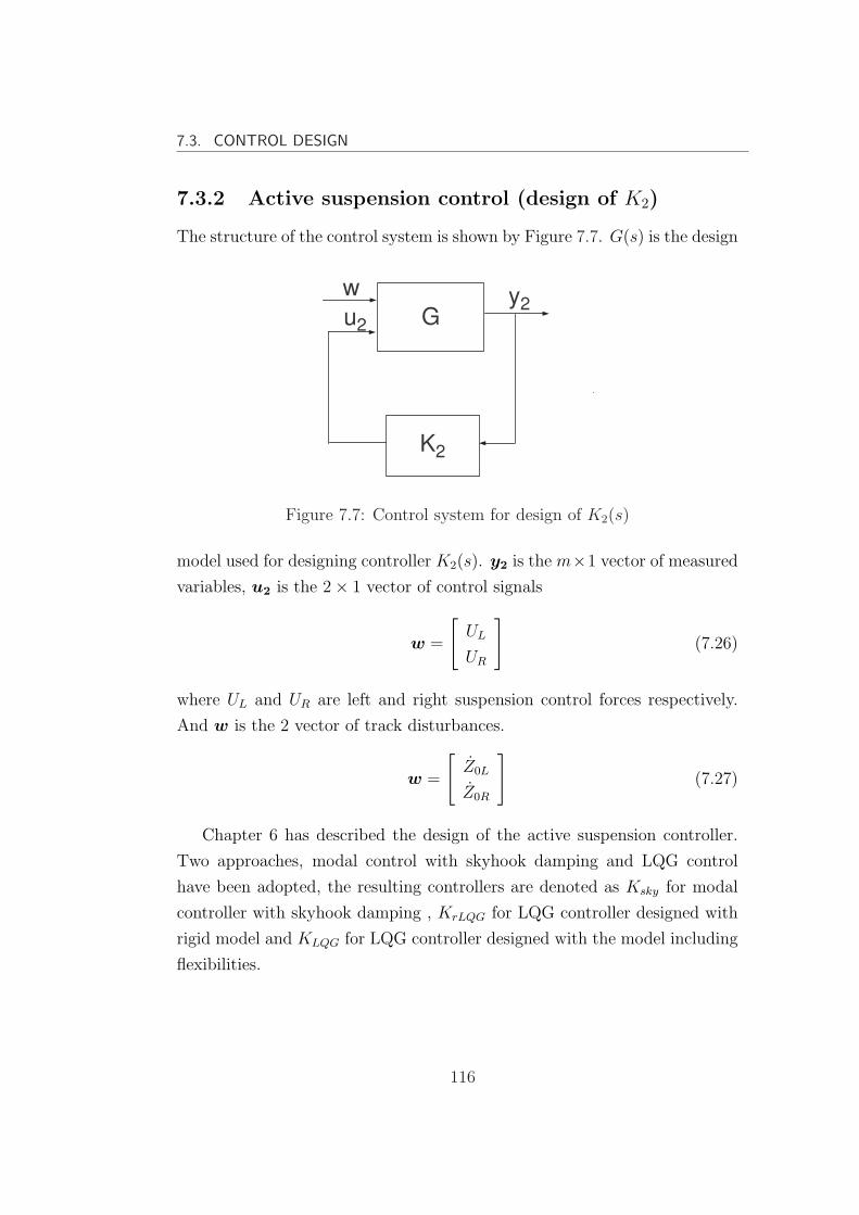
7.3. CONTROL DESIGN
7.3.2 Active suspension control (design of K2)
The structure of the control system is shown by Figure 7.7. G(s) is the design
G
K2
w
u2
y2
Figure 7.7: Control system for design of K2(s)
model used for designing controller K2(s). y2 is the m×1 vector of measured
variables, u2 is the 2× 1 vector of control signals
w =
[UL
UR
](7.26)
where UL and UR are left and right suspension control forces respectively.
And w is the 2 vector of track disturbances.
w =
[Z0L
Z0R
](7.27)
Chapter 6 has described the design of the active suspension controller.
Two approaches, modal control with skyhook damping and LQG control
have been adopted, the resulting controllers are denoted as Ksky for modal
controller with skyhook damping , KrLQG for LQG controller designed with
rigid model and KLQG for LQG controller designed with the model including
flexibilities.
116
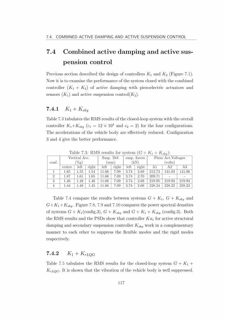
7.4. COMBINED ACTIVE DAMPING AND ACTIVE SUSPENSION CONTROL
7.4 Combined active damping and active sus-
pension control
Previous section described the design of controllers K1 and K2 (Figure 7.1).
Now it is to examine the performance of the system closed with the combined
controller (K1 + K2) of active damping with piezoelectric actuators and
sensors (K1) and active suspension control(K2).
7.4.1 K1 + Ksky
Table 7.3 tabulates the RMS results of the closed-loop system with the overall
controller K1+Ksky (c1 = 12 × 104 and c2 = 2) for the four configurations.
The accelerations of the vehicle body are effectively reduced. Configuration
3 and 4 give the better performance.
Table 7.3: RMS results for system (G + K1 + Ksky):
conf.Vertical Acc. Susp. Def. susp. forces Piezo Act.Voltages
(%g) (mm) (kN) (volts)centre left right left right left right A1 A2 A3
1 1.65 1.55 1.54 11.66 7.09 3.74 2.69 212.73 141.03 141.062 1.87 1.61 1.65 11.66 7.09 3.74 2.70 209.71 - -3 1.46 1.48 1.46 11.66 7.09 3.74 2.68 219.95 219.93 219.934 1.44 1.48 1.45 11.66 7.09 3.74 2.68 228.24 228.22 228.22
Table 7.4 compare the results between systems G + K1, G + Ksky and
G+K1+Ksky. Figure 7.8, 7.9 and 7.10 compares the power spectral densities
of systems G + K1(config.3), G + Ksky and G + K1 + Ksky (config.3). Both
the RMS results and the PSDs show that controller Ka1 for active structural
damping and secondary suspension controller Ksky work in a complementary
manner to each other to suppress the flexible modes and the rigid modes
respectively.
7.4.2 K1 + KrLQG
Table 7.5 tabulates the RMS results for the closed-loop system G + K1 +
KrLQG. It is shown that the vibration of the vehicle body is well suppressed.
117
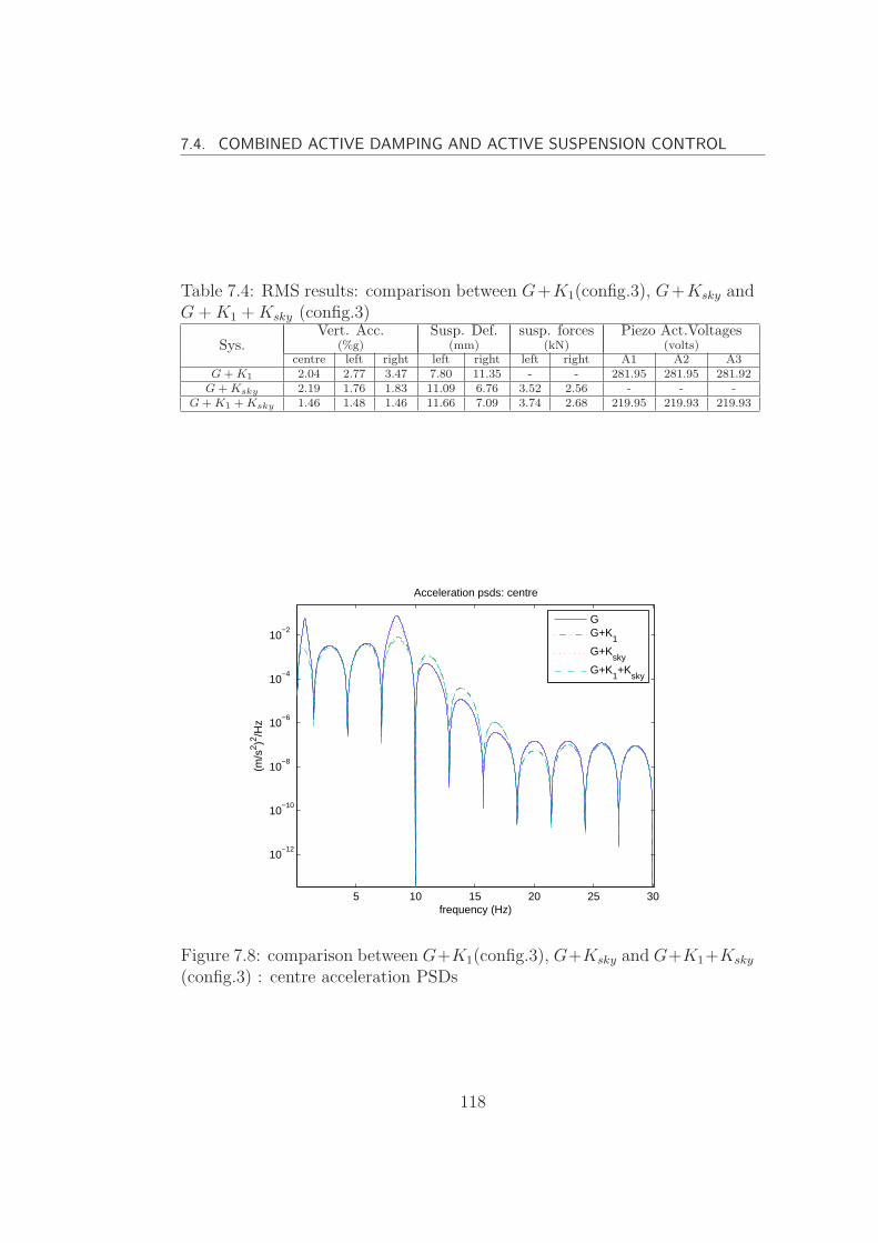
7.4. COMBINED ACTIVE DAMPING AND ACTIVE SUSPENSION CONTROL
Table 7.4: RMS results: comparison between G+K1(config.3), G+Ksky andG + K1 + Ksky (config.3)
Sys.Vert. Acc. Susp. Def. susp. forces Piezo Act.Voltages
(%g) (mm) (kN) (volts)centre left right left right left right A1 A2 A3
G + K1 2.04 2.77 3.47 7.80 11.35 - - 281.95 281.95 281.92G + Ksky 2.19 1.76 1.83 11.09 6.76 3.52 2.56 - - -
G + K1 + Ksky 1.46 1.48 1.46 11.66 7.09 3.74 2.68 219.95 219.93 219.93
5 10 15 20 25 30
10−12
10−10
10−8
10−6
10−4
10−2
Acceleration psds: centre
frequency (Hz)
(m/s
2 )2 /Hz
GG+K
1
G+Ksky
G+K1+K
sky
Figure 7.8: comparison between G+K1(config.3), G+Ksky and G+K1+Ksky
(config.3) : centre acceleration PSDs
118
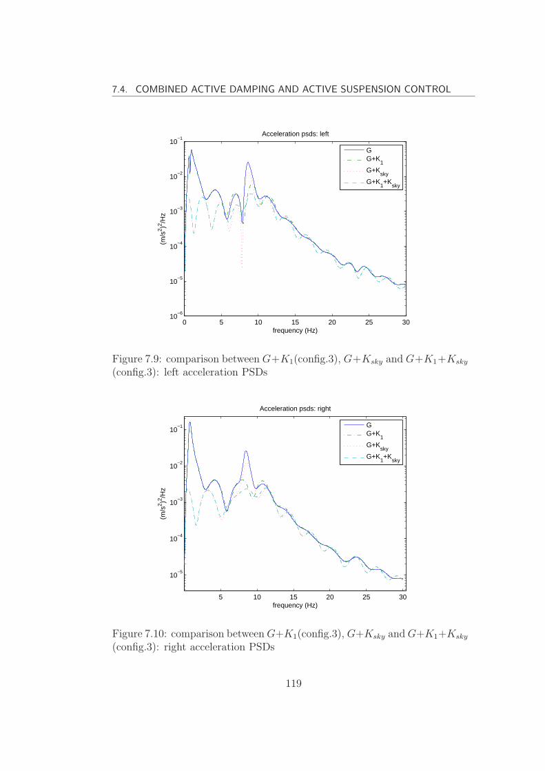
7.4. COMBINED ACTIVE DAMPING AND ACTIVE SUSPENSION CONTROL
0 5 10 15 20 25 3010
−6
10−5
10−4
10−3
10−2
10−1
Acceleration psds: left
frequency (Hz)
(m/s
2 )2 /Hz
GG+K
1
G+Ksky
G+K1+K
sky
Figure 7.9: comparison between G+K1(config.3), G+Ksky and G+K1+Ksky
(config.3): left acceleration PSDs
5 10 15 20 25 30
10−5
10−4
10−3
10−2
10−1
Acceleration psds: right
frequency (Hz)
(m/s
2 )2 /Hz
GG+K
1
G+Ksky
G+K1+K
sky
Figure 7.10: comparison between G+K1(config.3), G+Ksky and G+K1+Ksky
(config.3): right acceleration PSDs
119
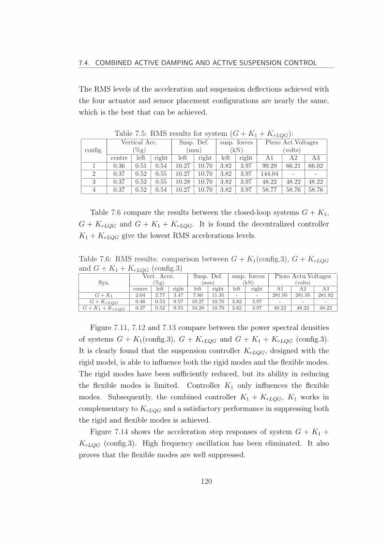
7.4. COMBINED ACTIVE DAMPING AND ACTIVE SUSPENSION CONTROL
The RMS levels of the acceleration and suspension deflections achieved with
the four actuator and sensor placement configurations are nearly the same,
which is the best that can be achieved.
Table 7.5: RMS results for system (G + K1 + KrLQG):
config.Vertical Acc. Susp. Def. susp. forces Piezo Act.Voltages
(%g) (mm) (kN) (volts)centre left right left right left right A1 A2 A3
1 0.36 0.51 0.54 10.27 10.70 3.82 3.97 99.29 66.21 66.022 0.37 0.52 0.55 10.27 10.70 3.82 3.97 144.04 - -3 0.37 0.52 0.55 10.28 10.70 3.82 3.97 48.22 48.22 48.224 0.37 0.52 0.54 10.27 10.70 3.82 3.97 58.77 58.76 58.76
Table 7.6 compare the results between the closed-loop systems G + K1,
G + KrLQG and G + K1 + KrLQG. It is found the decentralized controller
K1 + KrLQG give the lowest RMS accelerations levels.
Table 7.6: RMS results: comparison between G + K1(config.3), G + KrLQG
and G + K1 + KrLQG (config.3)
Sys.Vert. Acce. Susp. Def. susp. forces Piezo Actu.Voltages
(%g) (mm) (kN) (volts)centre left right left right left right A1 A2 A3
G + K1 2.04 2.77 3.47 7.80 11.35 - - 281.95 281.95 281.92G + KrLQG 0.46 0.53 0.57 10.27 10.70 3.82 3.97 - - -
G + K1 + KrLQG 0.37 0.52 0.55 10.28 10.70 3.82 3.97 48.22 48.22 48.22
Figure 7.11, 7.12 and 7.13 compare between the power spectral densities
of systems G + K1(config.3), G + KrLQG and G + K1 + KrLQG (config.3).
It is clearly found that the suspension controller KrLQG, designed with the
rigid model, is able to influence both the rigid modes and the flexible modes.
The rigid modes have been sufficiently reduced, but its ability in reducing
the flexible modes is limited. Controller K1 only influences the flexible
modes. Subsequently, the combined controller K1 + KrLQG, K1 works in
complementary to KrLQG and a satisfactory performance in suppressing both
the rigid and flexible modes is achieved.
Figure 7.14 shows the acceleration step responses of system G + K1 +
KrLQG (config.3). High frequency oscillation has been eliminated. It also
proves that the flexible modes are well suppressed.
120
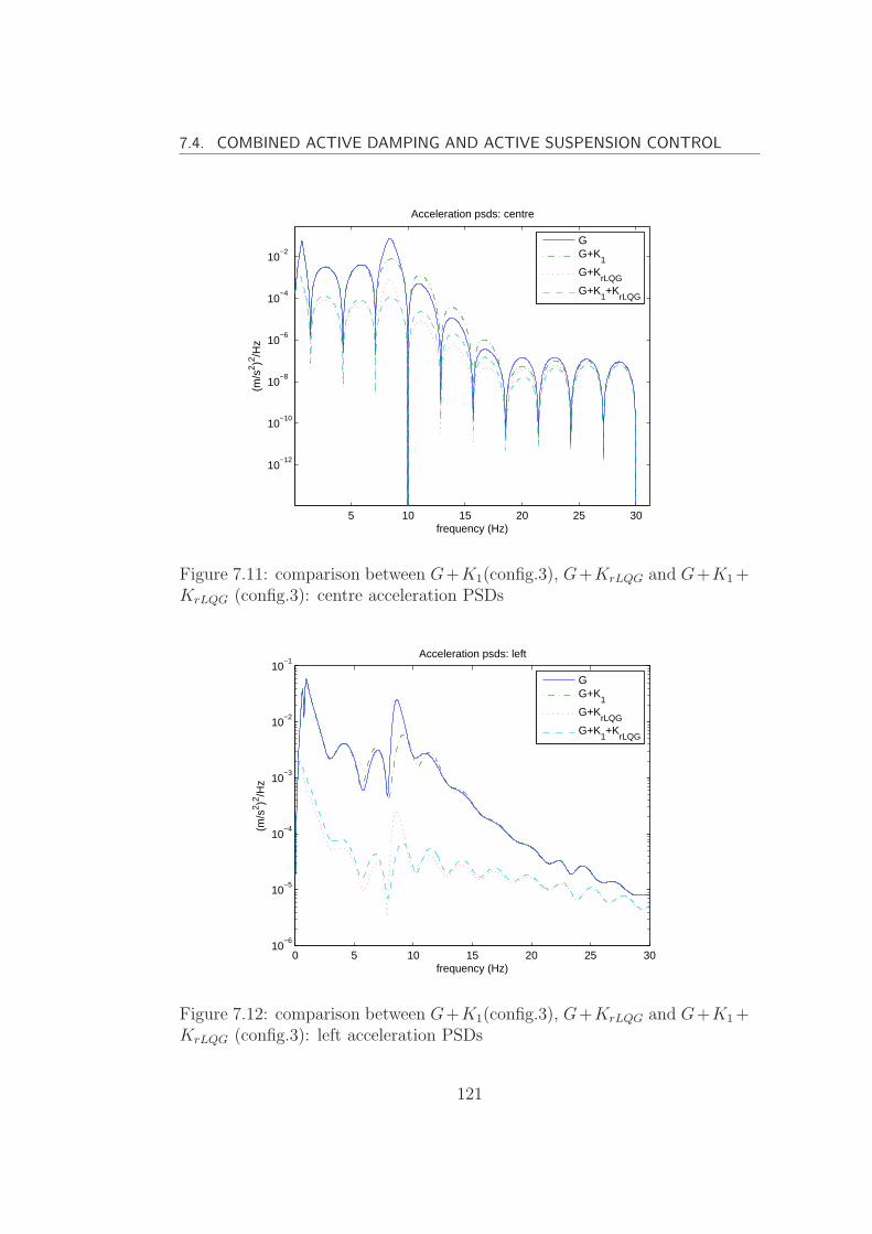
7.4. COMBINED ACTIVE DAMPING AND ACTIVE SUSPENSION CONTROL
5 10 15 20 25 30
10−12
10−10
10−8
10−6
10−4
10−2
Acceleration psds: centre
frequency (Hz)
(m/s
2 )2 /Hz
GG+K
1
G+KrLQG
G+K1+K
rLQG
Figure 7.11: comparison between G+K1(config.3), G+KrLQG and G+K1 +KrLQG (config.3): centre acceleration PSDs
0 5 10 15 20 25 3010
−6
10−5
10−4
10−3
10−2
10−1
Acceleration psds: left
frequency (Hz)
(m/s
2 )2 /Hz
GG+K
1
G+KrLQG
G+K1+K
rLQG
Figure 7.12: comparison between G+K1(config.3), G+KrLQG and G+K1 +KrLQG (config.3): left acceleration PSDs
121
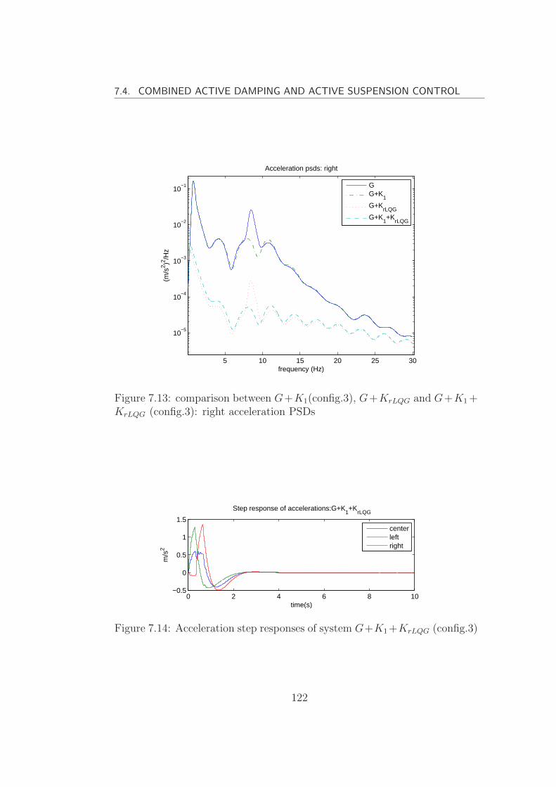
7.4. COMBINED ACTIVE DAMPING AND ACTIVE SUSPENSION CONTROL
5 10 15 20 25 30
10−5
10−4
10−3
10−2
10−1
Acceleration psds: right
frequency (Hz)
(m/s
2 )2 /Hz
GG+K
1
G+KrLQG
G+K1+K
rLQG
Figure 7.13: comparison between G+K1(config.3), G+KrLQG and G+K1 +KrLQG (config.3): right acceleration PSDs
0 2 4 6 8 10−0.5
0
0.5
1
1.5
Step response of accelerations:G+K1+K
rLQG
time(s)
m/s
2
centerleftright
Figure 7.14: Acceleration step responses of system G+K1+KrLQG (config.3)
122

7.4. COMBINED ACTIVE DAMPING AND ACTIVE SUSPENSION CONTROL
7.4.3 K1 + KLQG
KLQG is the suspension controller designed with the model including
flexibilities. RMS results of system G+KLQG and G+K1 +KLQG (config.3)
are tabulated in Table 7.7. Controller K1 + KLQG provides little further
improvement in ride quality compared with controller KLQG, because both
the rigid modes and flexible modes have already been well suppressed by
controller KLQG. In consequence, the voltage inputs to the piezoelectric
actuators for system G + K1 + KLQG are much smaller than the voltage
inputs for system G + K1. Figure 7.15,7.16 and 7.17 are acceleration PSDs
of systems G + K1, G + KLQG and G + K1 + KLQG.
Table 7.7: RMS results: comparison between G+KLQG and G+K1 +KLQG
(config.3)
Sys.Vert. Acce. Susp. Def. Susp. forces Piezo Actu.Voltages
(%g) (mm) (kN) (volts)centre left right left right left right A1 A2 A3
G + KLQG 0.36 0.50 0.54 10.33 10.79 3.87 4.02 - - -G + K1 + KLQG 0.35 0.51 0.54 10.34 10.79 3.87 4.02 33.90 33.89 33.89
5 10 15 20 25 30
10−10
10−5
Acceleration psds: centre
frequency (Hz)
(m/s
2 )2 /Hz
GG+K
1
G+KLQG
G+K1+K
LQG
Figure 7.15: comparison between G+K1(config.3), G+KLQG and G+K1 +KLQG (config.3): centre acceleration PSDs
123
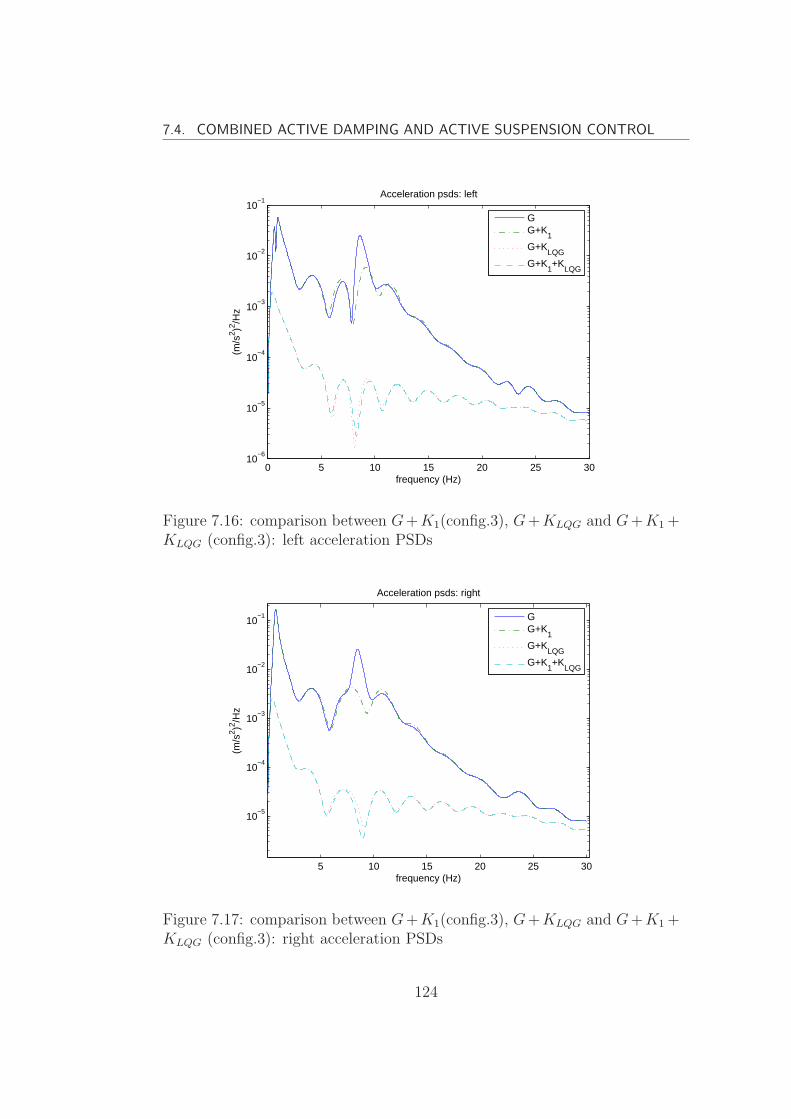
7.4. COMBINED ACTIVE DAMPING AND ACTIVE SUSPENSION CONTROL
0 5 10 15 20 25 3010
−6
10−5
10−4
10−3
10−2
10−1
Acceleration psds: left
frequency (Hz)
(m/s
2 )2 /Hz
GG+K
1
G+KLQG
G+K1+K
LQG
Figure 7.16: comparison between G+K1(config.3), G+KLQG and G+K1 +KLQG (config.3): left acceleration PSDs
5 10 15 20 25 30
10−5
10−4
10−3
10−2
10−1
Acceleration psds: right
frequency (Hz)
(m/s
2 )2 /Hz
GG+K
1
G+KLQG
G+K1+K
LQG
Figure 7.17: comparison between G+K1(config.3), G+KLQG and G+K1 +KLQG (config.3): right acceleration PSDs
124
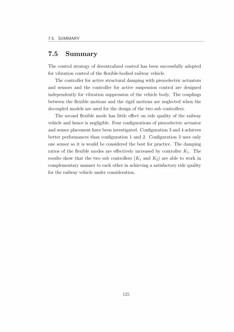
7.5. SUMMARY
7.5 Summary
The control strategy of decentralized control has been successfully adopted
for vibration control of the flexible-bodied railway vehicle.
The controller for active structural damping with piezoelectric actuators
and sensors and the controller for active suspension control are designed
independently for vibration suppression of the vehicle body. The couplings
between the flexible motions and the rigid motions are neglected when the
decoupled models are used for the design of the two sub controllers.
The second flexible mode has little effect on ride quality of the railway
vehicle and hence is negligible. Four configurations of piezoelectric actuator
and sensor placement have been investigated. Configuration 3 and 4 achieves
better performances than configuration 1 and 2. Configuration 3 uses only
one sensor so it is would be considered the best for practice. The damping
ratios of the flexible modes are effectively increased by controller K1. The
results show that the two sub controllers (K1 and K2) are able to work in
complementary manner to each other in achieving a satisfactory ride quality
for the railway vehicle under consideration.
125
Chapter 8
Control Design II: Centralized
Control
This chapter describes the centralized control strategy for vibration control
of the flexible bodied railway vehicle. The control inputs consist of
suspension control inputs and control inputs for active structural damping
by piezoelectric actuators. The full model of the system is used for control
design, which includes the rigid modes and flexible modes of the vehicle body
and the coupling terms of the flexible and rigid modes. Three control methods
will be considered : H2 optimal control, H∞ control and finally model
predictive control technology based on mixed H2/H∞ control approach.
8.1 Structure of centralized control
The structure of the centralized control strategy is shown in Figure 8.1, The
full model G(s) is used as design model. In state-space form, it is represented
as follows
x = Ax + B1ω + B2u (8.1)
(8.2)
126

8.1. STRUCTURE OF CENTRALIZED CONTROL
where the state vector x is chosen as
x = [Z3C θ Z1L Z1R Z3L − Z1L Z3R − Z1R Z2L − Z1L Z2R − Z1R
Z1L − Z0L Z1R − Z0R q1 q1 q2 q2] (8.3)
where A, B1 and B2 are the system matrix, track disturbance input matrix
and control input matrix respectively.
G(s)
K
w
uym
Figure 8.1: Structure of centralized control
ω is the vector of exogenous inputs, which includes the track disturbances
and the measurements noises, ym is the vector of measurement outputs. The
accelerations of the vehicle body are measured. u is the vector of control
inputs and is as below
u =
[u1
u2
](8.4)
where u1 is the vector of suspension control inputs and u2 is the vector of
voltage inputs to the piezoelectric actuators. As it is shown by Figure 8.2,
three sets of piezoelectric actuators are placed at the centre of the vehicle
body for suppressing the first flexible mode. On one common mounting
position, twenty piezoelectric stack actuators are placed in parallel in order
to produce the necessary moments. In this chapter, suppressing of the first
flexible mode, which is the dominant flexible mode that affects the ride
quality is, of the main concern.
K(s) is the centralized controller to be designed. The aim of the control
127
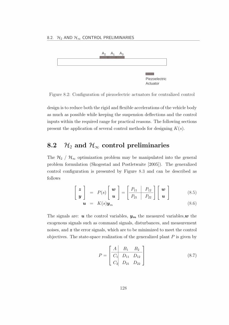
8.2. H2 AND H∞ CONTROL PRELIMINARIES
xxxxxxxxxxxxxxxxxxxxx
xxxxxxxxxxxxxxxxxxxxxxxx
xxxxxxxxxxxxxxxxxxxxx
A1A2 A3
xxxxxxxxxxxxxxxxxxxxx
Piezoelectric Actuator
Figure 8.2: Configuration of piezoelectric actuators for centralized control
design is to reduce both the rigid and flexible accelerations of the vehicle body
as much as possible while keeping the suspension deflections and the control
inputs within the required range for practical reasons. The following sections
present the application of several control methods for designing K(s).
8.2 H2 and H∞ control preliminaries
The H2 / H∞ optimization problem may be manipulated into the general
problem formulation (Skogestad and Postletwaite [2005]). The generalized
control configuration is presented by Figure 8.3 and can be described as
follows
[z
y
]= P (s)
[w
u
]=
[P11 P12
P21 P22
][w
u
](8.5)
u = K(s)ym (8.6)
The signals are: u the control variables, ym the measured variables,w the
exogenous signals such as command signals, disturbances, and measurement
noises, and z the error signals, which are to be minimized to meet the control
objectives. The state-space realization of the generalized plant P is given by
P =
A B1 B2
C1 D11 D12
C2 D21 D22
(8.7)
128
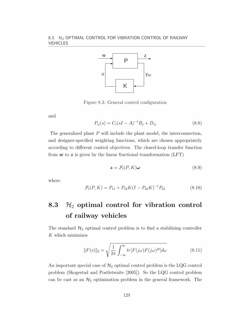
8.3. H2 OPTIMAL CONTROL FOR VIBRATION CONTROL OF RAILWAYVEHICLES
P
K
w z
u ym
Figure 8.3: General control configuration
and
Pij(s) = Ci(sI − A)−1Bj + Dij (8.8)
The generalized plant P will include the plant model, the interconnection,
and designer-specified weighting functions, which are chosen appropriately
according to different control objectives. The closed-loop transfer function
from w to z is given by the linear fractional transformation (LFT)
z = Fl(P, K)ω (8.9)
where
Fl(P, K) = P11 + P12K(I − P22K)−1P21 (8.10)
8.3 H2 optimal control for vibration control
of railway vehicles
The standard H2 optimal control problem is to find a stabilizing controller
K which minimizes
‖F (s)‖2 =
√1
2π
∫ ∞
−∞tr[F (jω)F (jω)H ]dω (8.11)
An important special case of H2 optimal control problem is the LQG control
problem (Skogestad and Postletwaite [2005]). So the LQG control problem
can be cast as an H2 optimization problem in the general framework. The
129
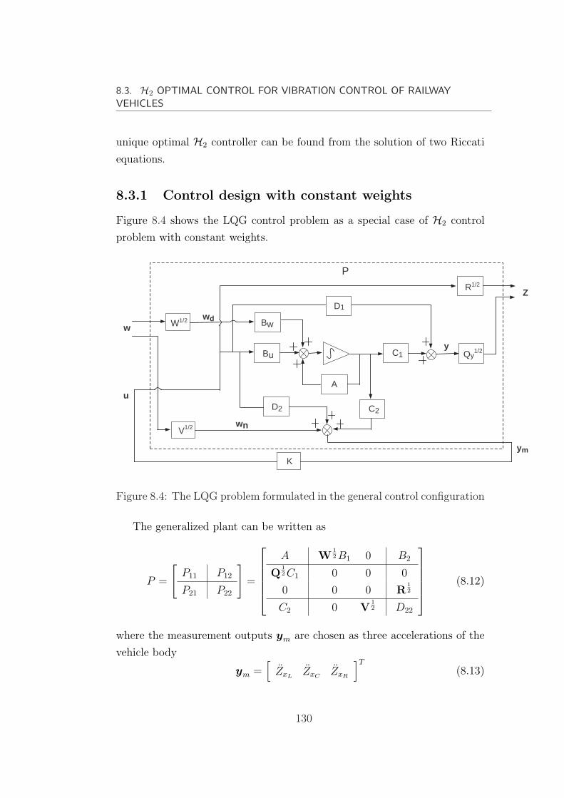
8.3. H2 OPTIMAL CONTROL FOR VIBRATION CONTROL OF RAILWAYVEHICLES
unique optimal H2 controller can be found from the solution of two Riccati
equations.
8.3.1 Control design with constant weights
Figure 8.4 shows the LQG control problem as a special case of H2 control
problem with constant weights.
Bu
A
C1
D1
C2
Bw
Qy1/2
D2
K
V1/2
W1/2
R1/2
Z
ym
wn
wwd
P
u
y
Figure 8.4: The LQG problem formulated in the general control configuration
The generalized plant can be written as
P =
[P11 P12
P21 P22
]=
A W12 B1 0 B2
Q12 C1 0 0 0
0 0 0 R12
C2 0 V12 D22
(8.12)
where the measurement outputs ym are chosen as three accelerations of the
vehicle body
ym =[
ZxLZxC
ZxR
]T
(8.13)
130

8.3. H2 OPTIMAL CONTROL FOR VIBRATION CONTROL OF RAILWAYVEHICLES
Piezoelectric sensors are not used in the centralized control design strategy.
The three accelerations will not only pick up the accelerations of the rigid
modes but also the flexibility effect associated with the three points (centre
xC , left xL and right xR).
The control input vector u is given as below
u =[
UL UR Va1 Va2 Va3
]T
(8.14)
where UL and UR are the command forces for the secondary suspension
actuators, and Va1, Va2 and Va3 are the voltage inputs to the piezoelectric
actuators. Here the actuators are all assumed ideal for controller design.
wd the vector of track disturbances, wn the vector of measurement noises
and w the vector of white noises of unit intensity are related by
[wd
wn
]=
[W
12 0
0 V12
]w (8.15)
where weights W and V are the covariances of wd and wn respectively. They
are chosen as ( please relate to the principles given in section 6.2.2).
W =
[5.4283× 10⁻⁴ 0
0 5.4283× 10⁻⁴
](8.16)
V =
1.3323× 10⁻⁵ 0 0
0 1.3323× 10⁻⁵ 0
0 0 1.3323× 10⁻⁵
(8.17)
The error signals z are the weighted regulated variables
z =
[Q
12y 0
0 R12
][y
u
](8.18)
where output variables y1 and the control inputs u are chosen as the
regulated variables, i.e. three accelerations of the vehicle body, two
131
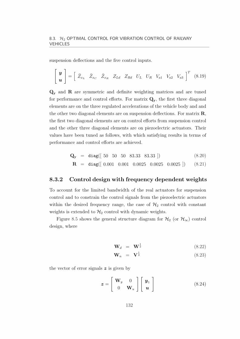
8.3. H2 OPTIMAL CONTROL FOR VIBRATION CONTROL OF RAILWAYVEHICLES
suspension deflections and the five control inputs.
[y
u
]=
[ZxL
ZxCZxR
ZLd ZRd UL UR Va1 Va2 Va3
]T
(8.19)
Qy and R are symmetric and definite weighting matrices and are tuned
for performance and control efforts. For matrix Qy, the first three diagonal
elements are on the three regulated accelerations of the vehicle body and and
the other two diagonal elements are on suspension deflections. For matrix R,
the first two diagonal elements are on control efforts from suspension control
and the other three diagonal elements are on piezoelectric actuators. Their
values have been tuned as follows, with which satisfying results in terms of
performance and control efforts are achieved.
Qy = diag([ 50 50 50 83.33 83.33 ]) (8.20)
R = diag([ 0.001 0.001 0.0025 0.0025 0.0025 ]) (8.21)
8.3.2 Control design with frequency dependent weights
To account for the limited bandwidth of the real actuators for suspension
control and to constrain the control signals from the piezoelectric actuators
within the desired frequency range, the case of H2 control with constant
weights is extended to H2 control with dynamic weights.
Figure 8.5 shows the general structure diagram for H2 (or H∞) control
design, where
Wd = W12 (8.22)
Wn = V12 (8.23)
the vector of error signals z is given by
z =
[Wy 0
0 Wu
][y1
u
](8.24)
132
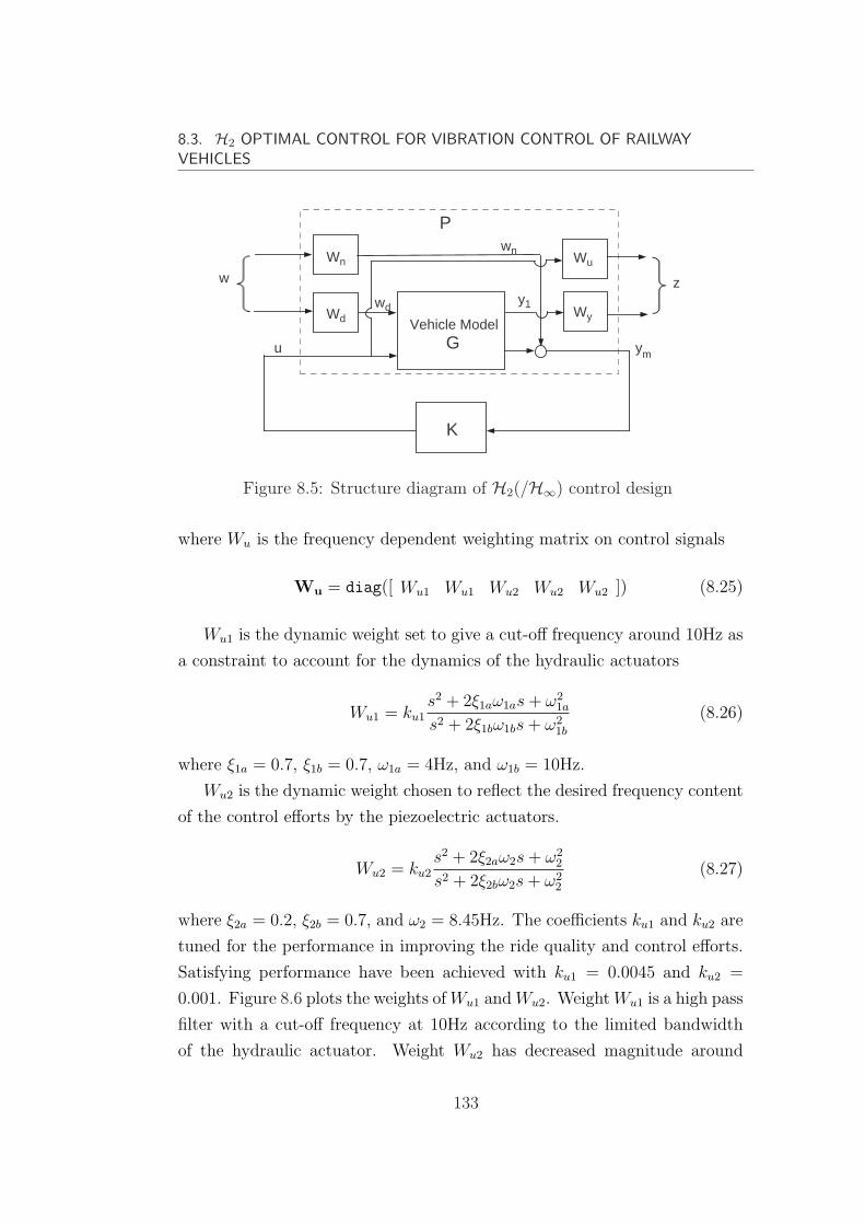
8.3. H2 OPTIMAL CONTROL FOR VIBRATION CONTROL OF RAILWAYVEHICLES
Wd
Wn Wu
WyVehicle Model G
K
ymu
w z
P
y1
wn
wd
Figure 8.5: Structure diagram of H2(/H∞) control design
where Wu is the frequency dependent weighting matrix on control signals
Wu = diag([ Wu1 Wu1 Wu2 Wu2 Wu2 ]) (8.25)
Wu1 is the dynamic weight set to give a cut-off frequency around 10Hz as
a constraint to account for the dynamics of the hydraulic actuators
Wu1 = ku1s2 + 2ξ1aω1as + ω2
1a
s2 + 2ξ1bω1bs + ω21b
(8.26)
where ξ1a = 0.7, ξ1b = 0.7, ω1a = 4Hz, and ω1b = 10Hz.
Wu2 is the dynamic weight chosen to reflect the desired frequency content
of the control efforts by the piezoelectric actuators.
Wu2 = ku2s2 + 2ξ2aω2s + ω2
2
s2 + 2ξ2bω2s + ω22
(8.27)
where ξ2a = 0.2, ξ2b = 0.7, and ω2 = 8.45Hz. The coefficients ku1 and ku2 are
tuned for the performance in improving the ride quality and control efforts.
Satisfying performance have been achieved with ku1 = 0.0045 and ku2 =
0.001. Figure 8.6 plots the weights of Wu1 and Wu2. Weight Wu1 is a high pass
filter with a cut-off frequency at 10Hz according to the limited bandwidth
of the hydraulic actuator. Weight Wu2 has decreased magnitude around
133

8.3. H2 OPTIMAL CONTROL FOR VIBRATION CONTROL OF RAILWAYVEHICLES
the frequency of 8.45Hz, which make the control efforts by the piezoelectric
actuators more concentrated on the first flexible mode of the vehicle body.
10−1
100
101
102
103
−75
−70
−65
−60
−55
−50
−45
Mag
nitu
de (
dB)
Weights on control inputs
Frequency (Hz)
Wu1
Wu2
Figure 8.6: Weights on control inputs for H2 control with ku1 = 0.004 andku2 = 0.001
8.3.3 Simulation results and analysis
This section analyzes the two H2 controllers designed above by constructing
the closed-loop feedback systems. We are interested in analyzing the
contribution of the piezoelectric actuators in further improving the ride
quality, so comparisons are made between the closed-loop system with and
without control from piezoelectric actuators.
Table 8.1 and Table 8.2 tabulate the RMS results of the accelerations of
the vehicle body, suspension deflections and control inputs. In general, the
vertical accelerations at these three positions of the vehicle body have been
effectively reduced by the H2 controllers. Due to the limitations placed by
the dynamic weights on the control inputs, it is not surprising to find that the
134
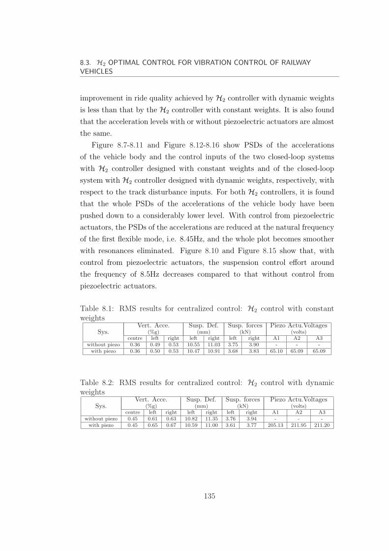
8.3. H2 OPTIMAL CONTROL FOR VIBRATION CONTROL OF RAILWAYVEHICLES
improvement in ride quality achieved by H2 controller with dynamic weights
is less than that by the H2 controller with constant weights. It is also found
that the acceleration levels with or without piezoelectric actuators are almost
the same.
Figure 8.7-8.11 and Figure 8.12-8.16 show PSDs of the accelerations
of the vehicle body and the control inputs of the two closed-loop systems
with H2 controller designed with constant weights and of the closed-loop
system with H2 controller designed with dynamic weights, respectively, with
respect to the track disturbance inputs. For both H2 controllers, it is found
that the whole PSDs of the accelerations of the vehicle body have been
pushed down to a considerably lower level. With control from piezoelectric
actuators, the PSDs of the accelerations are reduced at the natural frequency
of the first flexible mode, i.e. 8.45Hz, and the whole plot becomes smoother
with resonances eliminated. Figure 8.10 and Figure 8.15 show that, with
control from piezoelectric actuators, the suspension control effort around
the frequency of 8.5Hz decreases compared to that without control from
piezoelectric actuators.
Table 8.1: RMS results for centralized control: H2 control with constantweights
Sys.Vert. Acce. Susp. Def. Susp. forces Piezo Actu.Voltages
(%g) (mm) (kN) (volts)centre left right left right left right A1 A2 A3
without piezo 0.36 0.49 0.53 10.55 11.03 3.75 3.90 - - -with piezo 0.36 0.50 0.53 10.47 10.91 3.68 3.83 65.10 65.09 65.09
Table 8.2: RMS results for centralized control: H2 control with dynamicweights
Sys.Vert. Acce. Susp. Def. Susp. forces Piezo Actu.Voltages
(%g) (mm) (kN) (volts)centre left right left right left right A1 A2 A3
without piezo 0.45 0.61 0.63 10.82 11.35 3.76 3.94 - - -with piezo 0.45 0.65 0.67 10.59 11.00 3.61 3.77 205.13 211.95 211.20
135
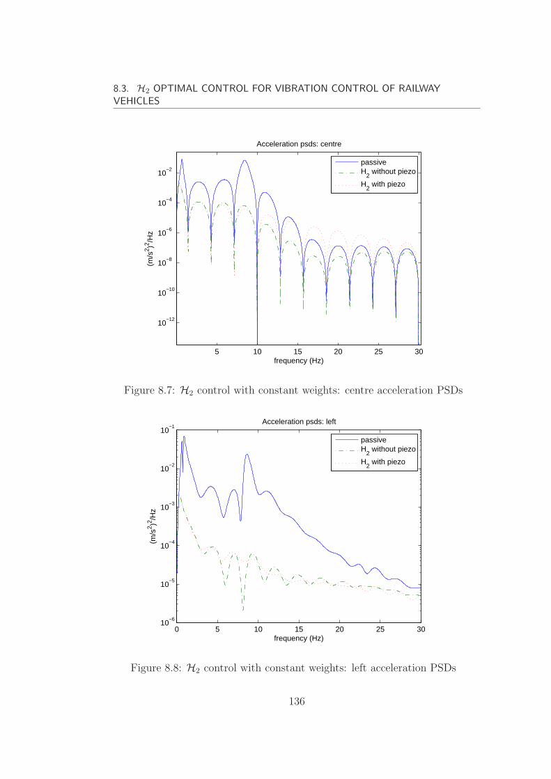
8.3. H2 OPTIMAL CONTROL FOR VIBRATION CONTROL OF RAILWAYVEHICLES
5 10 15 20 25 30
10−12
10−10
10−8
10−6
10−4
10−2
Acceleration psds: centre
frequency (Hz)
(m/s
2 )2 /Hz
passiveH
2 without piezo
H2 with piezo
Figure 8.7: H2 control with constant weights: centre acceleration PSDs
0 5 10 15 20 25 3010
−6
10−5
10−4
10−3
10−2
10−1
Acceleration psds: left
frequency (Hz)
(m/s
2 )2 /Hz
passiveH
2 without piezo
H2 with piezo
Figure 8.8: H2 control with constant weights: left acceleration PSDs
136
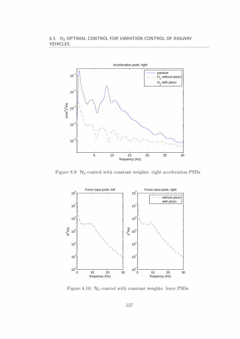
8.3. H2 OPTIMAL CONTROL FOR VIBRATION CONTROL OF RAILWAYVEHICLES
5 10 15 20 25 30
10−5
10−4
10−3
10−2
10−1
Acceleration psds: right
frequency (Hz)
(m/s
2 )2 /Hz
passiveH
2 without piezo
H2 with piezo
Figure 8.9: H2 control with constant weights: right acceleration PSDs
0 10 20 3010
2
103
104
105
106
107
108
Force input psds: left
frequency (Hz)
N2 /H
z
0 10 20 3010
2
103
104
105
106
107
108
Force input psds: right
frequency (Hz)
V2 /H
z
without piezowith piezo
Figure 8.10: H2 control with constant weights: force PSDs
137
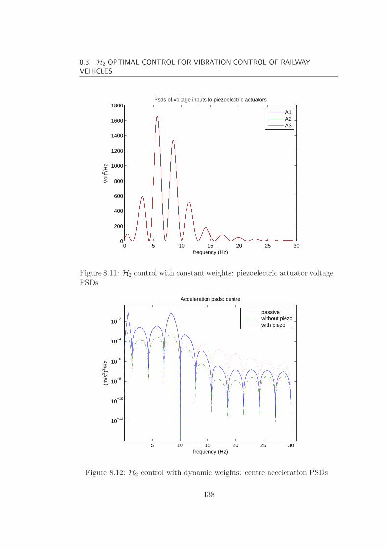
8.3. H2 OPTIMAL CONTROL FOR VIBRATION CONTROL OF RAILWAYVEHICLES
0 5 10 15 20 25 300
200
400
600
800
1000
1200
1400
1600
1800Psds of voltage inputs to piezoelectric actuators
frequency (Hz)
Vol
t2 /Hz
A1A2A3
Figure 8.11: H2 control with constant weights: piezoelectric actuator voltagePSDs
5 10 15 20 25 30
10−12
10−10
10−8
10−6
10−4
10−2
Acceleration psds: centre
frequency (Hz)
(m/s
2 )2 /Hz
passivewithout piezowith piezo
Figure 8.12: H2 control with dynamic weights: centre acceleration PSDs
138
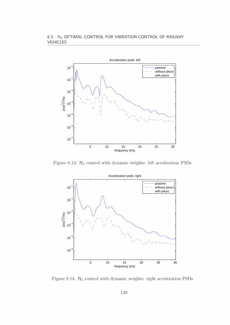
8.3. H2 OPTIMAL CONTROL FOR VIBRATION CONTROL OF RAILWAYVEHICLES
5 10 15 20 25 30
10−7
10−6
10−5
10−4
10−3
10−2
10−1
Acceleration psds: left
frequency (Hz)
(m/s
2 )2 /Hz
passivewithout piezowith piezo
Figure 8.13: H2 control with dynamic weights: left acceleration PSDs
5 10 15 20 25 30
10−6
10−5
10−4
10−3
10−2
10−1
Acceleration psds: right
frequency (Hz)
(m/s
2 )2 /Hz
passivewithout piezowith piezo
Figure 8.14: H2 control with dynamic weights: right acceleration PSDs
139
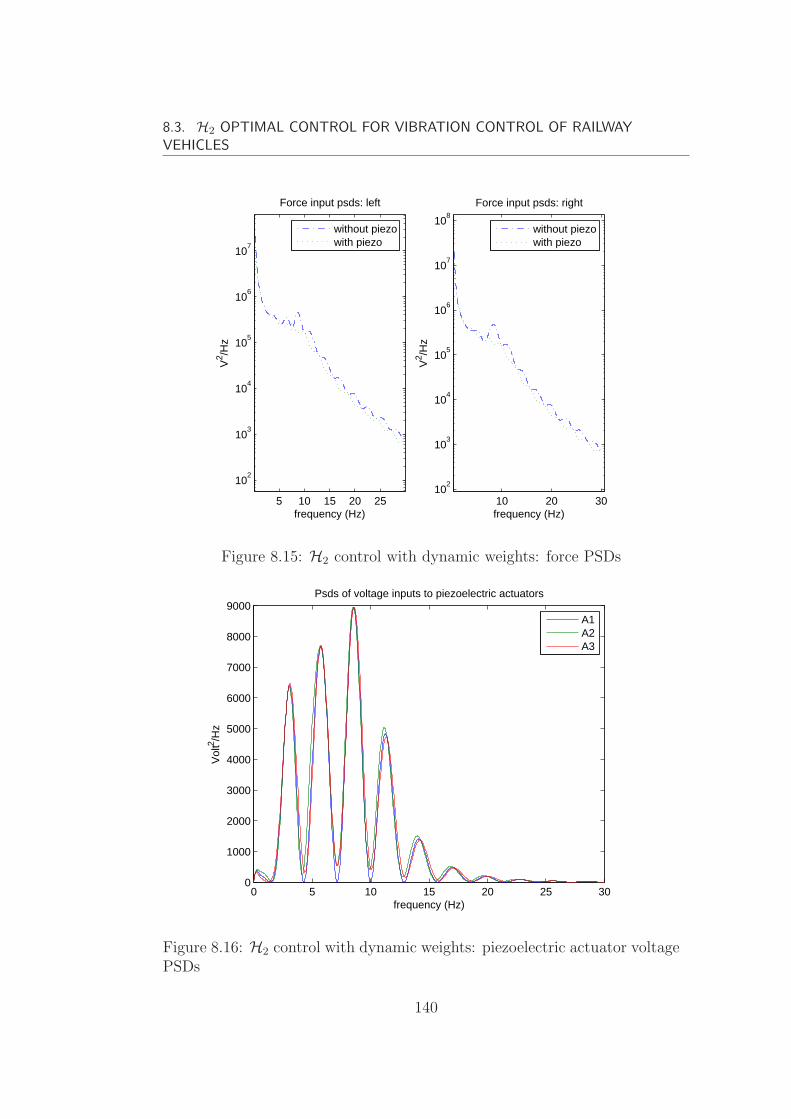
8.3. H2 OPTIMAL CONTROL FOR VIBRATION CONTROL OF RAILWAYVEHICLES
5 10 15 20 25
102
103
104
105
106
107
Force input psds: left
frequency (Hz)
V2 /H
z
without piezowith piezo
10 20 3010
2
103
104
105
106
107
108
Force input psds: right
frequency (Hz)
V2 /H
z
without piezowith piezo
Figure 8.15: H2 control with dynamic weights: force PSDs
0 5 10 15 20 25 300
1000
2000
3000
4000
5000
6000
7000
8000
9000Psds of voltage inputs to piezoelectric actuators
frequency (Hz)
Vol
t2 /Hz
A1A2A3
Figure 8.16: H2 control with dynamic weights: piezoelectric actuator voltagePSDs
140

8.4. H∞ OPTIMAL CONTROL FOR VIBRATION CONTROL OF RAILWAYVEHICLES
8.3.4 Summary
In this section, it has been shown that the designed H2 controllers have
successfully improved ride quality of the railway vehicle body against random
irregularities of the track. By tuning the coefficients of the weights, satisfying
acceleration levels are obtained in both the situations: with or without
piezoelectric actuators. With piezoelectric actuators, the control effort
around the frequencies of the first flexible mode decreases and the resonances
in PSDs of the accelerations are eliminated.
It is known that H2 controllers push down all the singular values over
all frequencies of the generalized plant. One of its shortcomings is that it
has poor robustness properties attributed to the integral criterion in terms
of the H2 norm. So next robust H∞ control technique will be considered for
vibration control of the flexible-bodied vehicle body.
8.4 H∞ optimal control for vibration control
of railway vehicles
The H∞ norm of a stable transfer function matrix G(jω) is defined as its
largest singular value over the entire frequency range
‖G(jω)‖∞ = supω
σ(G(jω)) (8.28)
where σ represents the largest singular value of G(jω).
For the H∞ based control design, the controller K(s) is selected in such a
way that it stabilizes the nominal system such that the H∞ norm of Fl(P, K)
is minimized or becomes smaller than a specified value γ.
minK∈S
‖Fl(P, K)‖∞ < γ (8.29)
Therefore, H∞ control pushes down the peak of the largest singular value.
Transfer function shaping approach (e.g. the mixed-sensitivity H∞ con-
trol) and the signal-based approach are the two distinguished methodologies
141
8.4. H∞ OPTIMAL CONTROL FOR VIBRATION CONTROL OF RAILWAYVEHICLES
for H∞ controller design. The first methodology focuses on the size and
bandwidth of the selected closed-loop transfer functions while the later
focuses on the size of the error signals. The problem can be solved either by
Riccati based approach or linear matrix inequalities (LMI) based approach.
The computation required for designing H∞ controllers can be intense but
the solution of the controller can be calculated with the available software
MATLAB. One of the difficulty is the selection of weights, which is aimed to
provide a good trade-off between conflicting objectives in various frequency
ranges.
8.4.1 Choice of weight
The signal-based approach is used for designing the H∞ controller. The
diagram for generalized plant for H∞ control is given by Figure 8.5. The
robust H∞ controllers are to be designed with the nominal plant without
considering the system uncertainty.
The control inputs u, measurement outputs ym and regulated variables
are chosen as following
u =[
UL UR Va1 Va2 Va3
]T
(8.30)
ym =[
ZxLZxC
ZxR
]T
(8.31)
[y
u
]=
[ZxL
ZxCZxR
ZLd ZRd UL UR Va1 Va2 Va3
]T
(8.32)
where UL and UR are the force commands for the secondary suspension
actuators, and Va1, Va2 and Va3 are the voltage inputs to the piezoelectric
actuators. ZxL, ZxC
and ZxRare the three body accelerations which will pick
up both the rigid accelerations and flexibility effect associated with the three
points xL, xC and xR.
Weights on the regulated variables are as follows
Wy = diag([ Wz1 Wz1 Wz1 kz2 kz2 )] (8.33)
142
8.4. H∞ OPTIMAL CONTROL FOR VIBRATION CONTROL OF RAILWAYVEHICLES
Wu = diag([ Wu1 Wu1 Wu2 Wu2 Wu2 ]) (8.34)
It is required that the first flexible mode be effectively reduced by the piezo-
electric actuators, so Wz1 the frequency dependent weight on accelerations,
as shown in Figure 8.5, are set to produce an increased gain at the frequencies
around 8.5Hz.
Wz1 = kz1s2 + 2ξ1cω2s + ω2
2
s2 + 2ξ1dω2s + ω22
(8.35)
where ξ1c = 0.7, ξ1d = 0.3 and ω2 = 8.45Hz.
Wu1 are frequency dependent weights on the suspension control inputs to
account for the limited bandwidth of the hydraulic actuators.
Wu1 = ku1s2 + 2ξ1aω1as + ω2
1a
s2 + 2ξ1bω1bs + ω21b
(8.36)
where ξ1a = 0.7, ξ1b = 0.7, ω1a = 4Hz, and ω1b = 10Hz.
Wu2 are frequency dependent weights chosen to reflect the desired
frequency content of the control efforts by the piezoelectric actuators.
Wu2 = ku2s2 + 2ξ2aω2s + ω2
2
s2 + 2ξ2bω2s + ω22
(8.37)
where ξ2a = 0.4, ξ2b = 0.7, and ω2 = 8.45Hz.
The constant weights kz2 and the coefficients kz1, ku1 and ku2 are tuned
for performance in improving the ride quality and control efforts. Figure 8.17
shows the weights of Wz1, Wu1 and Wu2 with kz1 = 50, ku1 = 0.0014 and
ku2 = 0.01, with which satisfying results have been achieved.
8.4.2 Simulation results
Table 8.3 tabulates the RMS results of acceleration levels, suspension
deflections, suspension control forces and voltages inputs for piezoelectric
actuators of the closed-loop system with the H∞ controller, which is solved
by LMI based approach, where C1 and C2 denote the two controllers without
piezoelectric inputs and with piezoelectric inputs respectively. It is shown
that only a small further reduction in acceleration levels have been achieved
143

8.4. H∞ OPTIMAL CONTROL FOR VIBRATION CONTROL OF RAILWAYVEHICLES
10−1
100
101
102
103
−80
−60
−40
−20
0
20
40
Mag
nitu
de (
dB)
Bode diagram
Frequency (Hz)
Wz1
Wu1
Wu2
Figure 8.17: Weights on outputs for H∞ control with kz1 = 33.33, kz2 = 50,ku1 = 0.0016 and ku2 = 0.005
144

8.4. H∞ OPTIMAL CONTROL FOR VIBRATION CONTROL OF RAILWAYVEHICLES
by including piezoelectric control inputs.
Table 8.3: RMS results for H∞ control
Sys.Vert. Acce. Susp. Def. susp. forces Piezo Actu.Voltages
(%g) (mm) (kN) (volts)centre left right left right left right A1 A2 A3
C1 0.69 0.83 0.78 8.91 9.54 3.2 3.61 - - -C2 0.57 0.67 0.62 9.59 9.56 3.50 3.78 100.94 103.05 101.26
Figure 8.18, 8.19, 8.20, 8.21 and 8.22 show PSDs for the centre, left
and right accelerations, suspension control inputs and piezoelectric control
inputs respectively of the closed-loop system with controllers C1 and C2 with
respect to random track disturbances. Comparing C1 and C2, accelerations
are further reduced with piezoelectric control inputs.
5 10 15 20 25 30
10−10
10−5
Acceleration psds: centre
frequency (Hz)
(m/s
2 )2 /Hz
passiveC
1
C2
Figure 8.18: H∞ control: centre acceleration PSDs
8.4.3 Summary
H∞ controllers are designed for vibration suppressing of the flexible-bodied
railway vehicle. The RMS results and the PSDs plots have shown that
145

8.4. H∞ OPTIMAL CONTROL FOR VIBRATION CONTROL OF RAILWAYVEHICLES
5 10 15 20 25 30
10−8
10−6
10−4
10−2
Acceleration psds: left
frequency (Hz)
(m/s
2 )2 /Hz
passiveC
1
C2
Figure 8.19: H∞ control: left acceleration PSDs
5 10 15 20 25 30
10−8
10−6
10−4
10−2
Acceleration psds: right
frequency (Hz)
(m/s
2 )2 /Hz
passiveC
1
C2
Figure 8.20: H∞ control: right acceleration PSDs
146
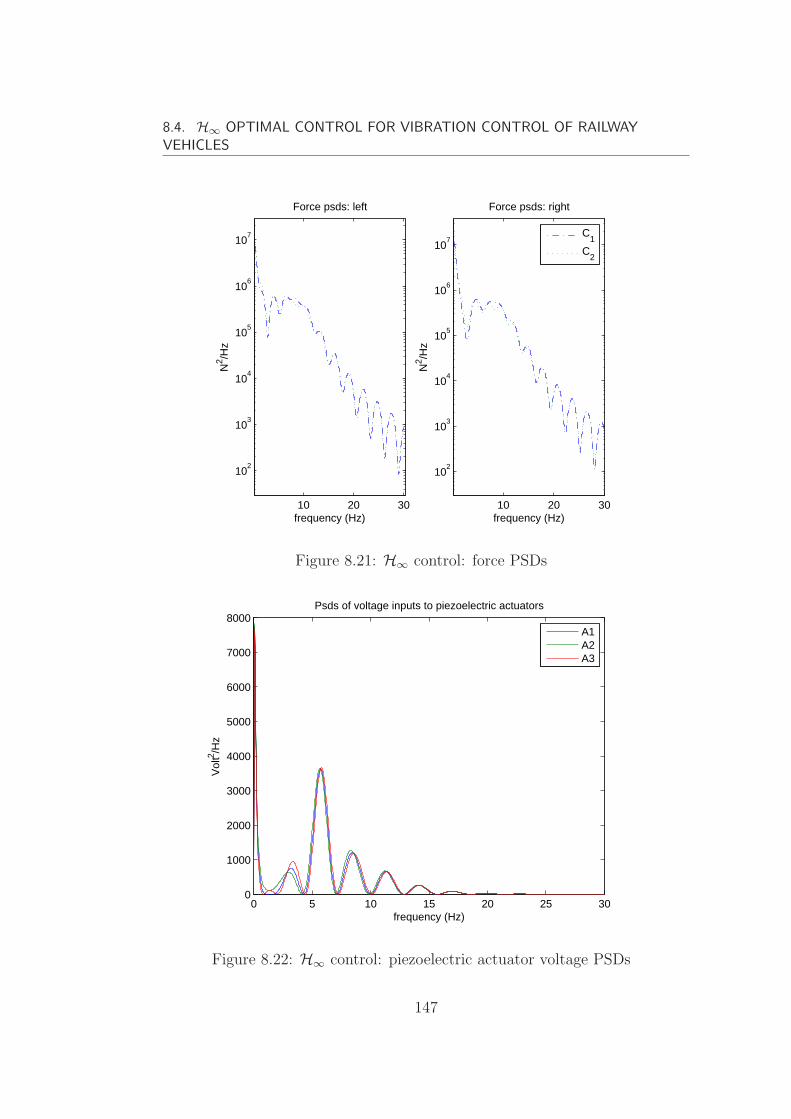
8.4. H∞ OPTIMAL CONTROL FOR VIBRATION CONTROL OF RAILWAYVEHICLES
10 20 30
102
103
104
105
106
107
Force psds: left
frequency (Hz)
N2 /H
z
10 20 30
102
103
104
105
106
107
Force psds: right
frequency (Hz)
N2 /H
z
C
1
C2
Figure 8.21: H∞ control: force PSDs
0 5 10 15 20 25 300
1000
2000
3000
4000
5000
6000
7000
8000Psds of voltage inputs to piezoelectric actuators
frequency (Hz)
Vol
t2 /Hz
A1A2A3
Figure 8.22: H∞ control: piezoelectric actuator voltage PSDs
147

8.5. MODEL PREDICTIVE CONTROL BASED ON MIXED H2/H∞ CONTROLAPPROACH FOR VIBRATION CONTROL OF RAILWAY VEHICLES
further reduction in accelerations is achieved with the inclusion of control
by piezoelectric actuators. One of the shortcomings of H∞ control is that
it can be conservative because H∞ norm of a system represents the worst-
case energy transfer between disturbances to regulated outputs and trade-
off exists between performance and robustness. In the next section, a new
control method based on mixed H2/H∞ control approach is going to be
introduced and applied to the vibration control problem of the flexible-bodied
railway vehicles.
8.5 Model predictive control based on mixed
H2/H∞ control approach for vibration
control of railway vehicles 1
This part of work is an application of model predictive control using mixed
H2/H∞ control approach for active vibration control of railway vehicles, with
the aim to improve the ride quality of the railway vehicle.
Model Predictive Control (MPC) technology based on mixed H2/H∞control approach (Orukpe et al. [2007]) is utilized for active vibration control
of a railway vehicle. The suitability of the proposed approach stems from
the fact of considering both performance and robustness issues within a
unified framework. The work is based on Linear Matrix Inequalities (LMI),
in particular develops an LMI linear in the state feedback. The interested
reader can see more details on LMIs in paper by Scherer and Weiland [2000]
. LMIs are inequalities linear in sets of matrix variables. From a control
engineering point of view, one of the main attractions of LMIs is that they
can be used to solve problems which involve several matrix variables, with
different structures imposed on these matrix variables. Another attractive
feature of LMI methods is that they form a flexible approach, thus it is usually
1This work was in collaboration with Dr. Patience E. Orupke, Imperial College London.A common paper was published, details: Patience E. Orukpe, X.Zheng, I.M.Jaimoukha,A.C.Zolotas and R.M.Goodall Model predictive control based on mixed control approachfor active vibration control of railway vehicles Vehicle System Dynamics, 46:1, 151-160,2008
148

8.5. MODEL PREDICTIVE CONTROL BASED ON MIXED H2/H∞ CONTROLAPPROACH FOR VIBRATION CONTROL OF RAILWAY VEHICLES
rather straightforward to pose a multitude of problems as LMI problems.
An advantage of LMIs is that they are able to unite many previous existing
results in a common framework. In this section, the potential of improving
the ride quality of the railway vehicle and overall performances of the system
will be investigated.
8.5.1 Control design
MPC is a form of control in which the current control action is obtained
by solving on-line, at each sampling instant, an open-loop optimal control
problem. Using the current states of the plant as the initial states; the
optimization yields an optimal control sequence and the first control in this
sequence is applied to the plant. The main advantages of MPC include the
ability to handle constraints and the capability for controlling multivariable
plants, although computational requirements increase due to the online
computation and problem dimension.
The following discrete-time state-space representation of the linear time
invariant railway vehicle model is considered
x(k + 1) = Ax(k) + B1w(k) + B2u(k)
y(k) = Cx(k) + D1ww(k) + D1uu(k)
z(k) =
[ √RLQu(k)√QLQy(k)
]
x(0) = x0 (8.38)
where the state x(k) ∈ R12 and the track disturbance w(k) ∈ R2 are the
same as given for flexible model in chapter 5. The control inputs, u(k) ∈ R5,
are
u =[
UL UR Va1 Va2 Va3
]T
(8.39)
where UL and UR are the command forces for the secondary suspension
actuators, and Va1, Va2 and Va3 are the voltage inputs to the piezoelectric
149
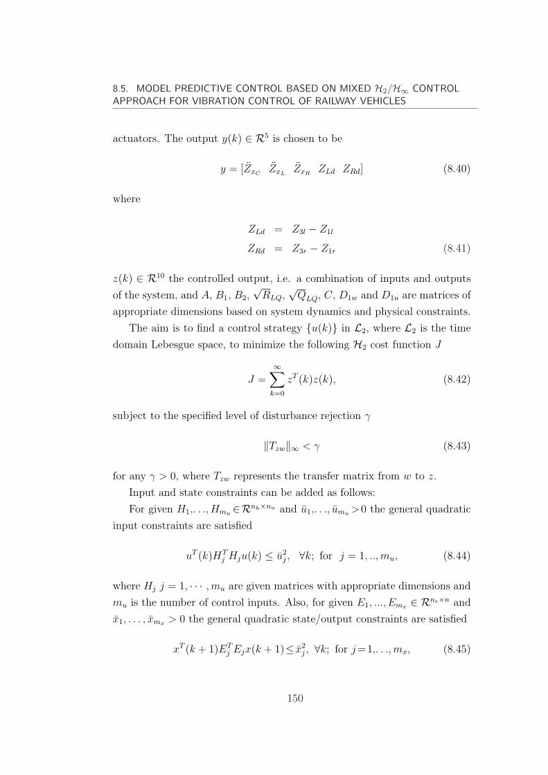
8.5. MODEL PREDICTIVE CONTROL BASED ON MIXED H2/H∞ CONTROLAPPROACH FOR VIBRATION CONTROL OF RAILWAY VEHICLES
actuators. The output y(k) ∈ R5 is chosen to be
y = [ZxCZxL
ZxRZLd ZRd] (8.40)
where
ZLd = Z3l − Z1l
ZRd = Z3r − Z1r (8.41)
z(k) ∈ R10 the controlled output, i.e. a combination of inputs and outputs
of the system, and A, B1, B2,√
RLQ,√
QLQ, C, D1w and D1u are matrices of
appropriate dimensions based on system dynamics and physical constraints.
The aim is to find a control strategy u(k) in L2, where L2 is the time
domain Lebesgue space, to minimize the following H2 cost function J
J =∞∑
k=0
zT (k)z(k), (8.42)
subject to the specified level of disturbance rejection γ
‖Tzw‖∞ < γ (8.43)
for any γ > 0, where Tzw represents the transfer matrix from w to z.
Input and state constraints can be added as follows:
For given H1,. . ., Hmu ∈Rnh×nu and u1,. . ., umu >0 the general quadratic
input constraints are satisfied
uT (k)HTj Hju(k) ≤ u2
j , ∀k; for j = 1, .., mu, (8.44)
where Hj j = 1, · · · ,mu are given matrices with appropriate dimensions and
mu is the number of control inputs. Also, for given E1, ..., Emx ∈ Rne×n and
x1, . . . , xmx > 0 the general quadratic state/output constraints are satisfied
xT (k + 1)ETj Ejx(k + 1)≤ x2
j , ∀k; for j =1,. . ., mx, (8.45)
150
8.5. MODEL PREDICTIVE CONTROL BASED ON MIXED H2/H∞ CONTROLAPPROACH FOR VIBRATION CONTROL OF RAILWAY VEHICLES
where Ej, j = 1, · · · ,mx are given matrices with appropriate dimensions and
mx is the number of states.
8.5.2 Problem Formulation
For state feedback u(k) = Fx(k), the state equation (8.38) becomes
x(k + 1) =
Acl︷ ︸︸ ︷(A + B2F ) x(k) + B1w(k).
The disturbance is assumed to be bounded by
∞∑
k=0
wT (k)w(k) ≤ w2,
or ‖w‖2 ≤ w.
The cost in (8.42) is considered and can be expressed as
J =xT0 Px0+γ2
∞∑
k=0
wT (k)w(k)+∞∑
k=0
[x(k)
w(k)
]T
K
[x(k)
w(k)
]
where K is defined as
K =
[k11 AT
clPB1 + F T DT1uQLQD1w + CT QLQD1w
BT1 PAcl + DT
1wQLQD1uF + DT1wQLQC BT
1 PB1 + DT1wQLQD1w − γ2I
]
(8.46)
where
k11 = ATclPAcl−P +CT QLQC+F T RLQF +2F T DT
1uQLQC+F T DT1uQLQD1uF
(8.47)
An application of the bounded real lemma (Dumitrescu [2005]) shows
that Acl is stable and (8.43) is satisfied if and only if K < 0 and P > 0.
These condition can be reduced to LMIs as shown in Theorem 8.5.1 below.
Thus the desired upper bound of the cost function is (for details of derivation,
151
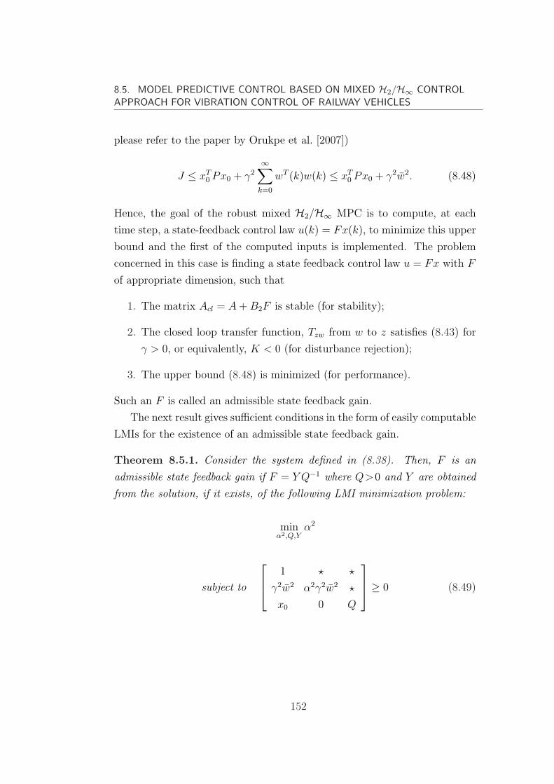
8.5. MODEL PREDICTIVE CONTROL BASED ON MIXED H2/H∞ CONTROLAPPROACH FOR VIBRATION CONTROL OF RAILWAY VEHICLES
please refer to the paper by Orukpe et al. [2007])
J ≤ xT0 Px0 + γ2
∞∑
k=0
wT (k)w(k) ≤ xT0 Px0 + γ2w2. (8.48)
Hence, the goal of the robust mixed H2/H∞ MPC is to compute, at each
time step, a state-feedback control law u(k) = Fx(k), to minimize this upper
bound and the first of the computed inputs is implemented. The problem
concerned in this case is finding a state feedback control law u = Fx with F
of appropriate dimension, such that
1. The matrix Acl = A + B2F is stable (for stability);
2. The closed loop transfer function, Tzw from w to z satisfies (8.43) for
γ > 0, or equivalently, K < 0 (for disturbance rejection);
3. The upper bound (8.48) is minimized (for performance).
Such an F is called an admissible state feedback gain.
The next result gives sufficient conditions in the form of easily computable
LMIs for the existence of an admissible state feedback gain.
Theorem 8.5.1. Consider the system defined in (8.38). Then, F is an
admissible state feedback gain if F = Y Q−1 where Q>0 and Y are obtained
from the solution, if it exists, of the following LMI minimization problem:
minα2,Q,Y
α2
subject to
1 ? ?
γ2w2 α2γ2w2 ?
x0 0 Q
≥ 0 (8.49)
152
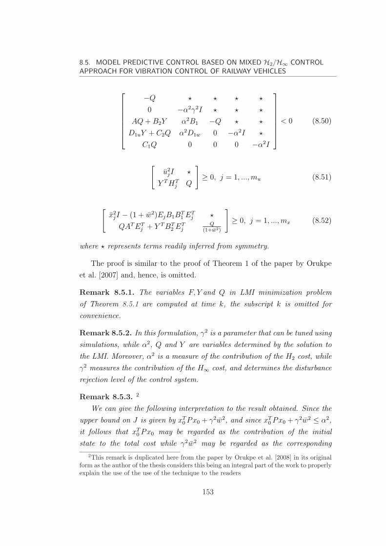
8.5. MODEL PREDICTIVE CONTROL BASED ON MIXED H2/H∞ CONTROLAPPROACH FOR VIBRATION CONTROL OF RAILWAY VEHICLES
−Q ? ? ? ?
0 −α2γ2I ? ? ?
AQ + B2Y α2B1 −Q ? ?
D1uY + C2Q α2D1w 0 −α2I ?
C1Q 0 0 0 −α2I
< 0 (8.50)
[u2
jI ?
Y T HTj Q
]≥ 0, j = 1, ..., mu (8.51)
[x2
jI − (1 + w2)EjB1BT1 ET
j ?
QAT ETj + Y T BT
2 ETj
Q(1+w2)
]≥ 0, j = 1, ..., mx (8.52)
where ? represents terms readily inferred from symmetry.
The proof is similar to the proof of Theorem 1 of the paper by Orukpe
et al. [2007] and, hence, is omitted.
Remark 8.5.1. The variables F, Y and Q in LMI minimization problem
of Theorem 8.5.1 are computed at time k, the subscript k is omitted for
convenience.
Remark 8.5.2. In this formulation, γ2 is a parameter that can be tuned using
simulations, while α2, Q and Y are variables determined by the solution to
the LMI. Moreover, α2 is a measure of the contribution of the H2 cost, while
γ2 measures the contribution of the H∞ cost, and determines the disturbance
rejection level of the control system.
Remark 8.5.3. 2
We can give the following interpretation to the result obtained. Since the
upper bound on J is given by xT0 Px0 + γ2w2, and since xT
0 Px0 + γ2w2 ≤ α2,
it follows that xT0 Px0 may be regarded as the contribution of the initial
state to the total cost while γ2w2 may be regarded as the corresponding
2This remark is duplicated here from the paper by Orukpe et al. [2008] in its originalform as the author of the thesis considers this being an integral part of the work to properlyexplain the use of the use of the technique to the readers
153
8.5. MODEL PREDICTIVE CONTROL BASED ON MIXED H2/H∞ CONTROLAPPROACH FOR VIBRATION CONTROL OF RAILWAY VEHICLES
contribution of the disturbance. By guaranteeing xT0 α−2Px0 + α−2γ2w2 ≤ 1,
this is a normalized mixed performance objective, where α−2γ2w2 is the
contribution of the H∞ cost and xT0 α−2Px0 is the contribution of the H2
cost. Therefore condition (8.49) might be considered as the normalized
mixed objective function. This is a more natural combination of the control
objectives since it emphasizes the trade-off between the normalized H2 cost
and the normalized H∞ bound.
8.5.3 Simulation results and discussion
In this simulation, we considered the discrete-time model of the railway
vehicle as given by (8.38), with a sampling time of 0.001 second. The static
state are taken as the initial state, so the initial values of the states are
x0 = [0; 0; 0; 0; 0; 0; 0; 0; 0; 0; 0; 0]. (8.53)
8.5.4 Parameter tuning
Tuning of RLQ and γ2
The term RLQ is given by
RLQ = diag([ r1 r1 r2 r2 r2 ]) (8.54)
The weight for suspension control inputs, r1 and the weight for voltage inputs
for piezoelectric actuators, r2, are tuned in order to achieve proper scaled
control inputs and the best performance for the system. The choice of γ2
is based on Remark 8.5.2. It measures the contribution of the H∞ cost in
(8.42), and determines the disturbance rejection level of the control system.
It is found that γ2 needs to be adjusted accordingly so that LMI could find
a feasible solution while it is desired to be small to maintain high disturbance
rejection level. For example, when stricter constraints on control inputs are
imposed with a relatively bigger value for r1 and r2, γ2 may need to be
increased too if LMI becomes infeasible.
154
8.5. MODEL PREDICTIVE CONTROL BASED ON MIXED H2/H∞ CONTROLAPPROACH FOR VIBRATION CONTROL OF RAILWAY VEHICLES
Tuning of QLQ
The term QLQ is given by
QLQ = diag[
q1 q1 q1 q2 q2
](8.55)
where q1 is the weight for accelerations and q2 is the weight for suspension
deflections. They are initially determined based on the physical constraints
of the system, and further tuned to achieve the best performance.
From experience, it is known that the requirements for acceleration and
suspension deflections are in conflict with each other. So when it shows
there is space for the deflections to be increased, weight q2 can be decreased
in order to achieve better ride quality. After changing the value for q2, it
may be necessary to go back to tune RLQ again as q2 will have an effect on
the control inputs too.
Results and discussion
Based on the principles given above, parameters of γ2, RLQ and QLQ are
chosen as: γ2 = 1000, r1 = 1 × 10⁻⁸, r2 = 1 × 10⁻⁷, q1 = 1/(0.15)2
and q2 = 1/(0.02)2. RMS results of the vertical accelerations in gravity%,
deflections in millimetres and control in Newton are are tabulated in Table
8.4. It shows that the accelerations of the vehicle body have been successfully
reduced with the designed controllers. With piezoelectric control, no obvious
further improvement in ride quality is found compared to the case without
piezoelectric control.
The time domain responses of the accelerations of the vehicle body and
control inputs to the random track disturbances are shown in Figure 8.23-
8.27. The PSDs of accelerations of the vehicle body, which are calculated in
time domain, are shown in Figure 8.28-8.30. The PDS results agrees with the
RMS results that the accelerations have been successfully reduced, however,
no big further improvements have been achieved by including piezoelectric
actuators for structural damping.
155
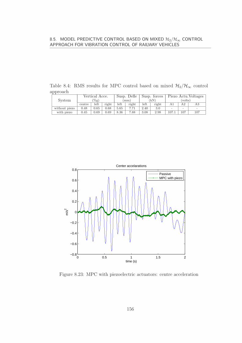
8.5. MODEL PREDICTIVE CONTROL BASED ON MIXED H2/H∞ CONTROLAPPROACH FOR VIBRATION CONTROL OF RAILWAY VEHICLES
Table 8.4: RMS results for MPC control based on mixed H2/H∞ controlapproach
SystemVertical Acce. Susp. Defle Susp. forces Piezo Actu.Voltages
(%g) (mm) (kN) (volts)centre left right left right left right A1 A2 A3
without piezo 0.48 0.65 0.68 5.65 7.71 2.40 3.0 - - -with piezo 0.45 0.69 0.69 8.36 7.88 3.08 2.98 107.1 107 107
0 0.5 1 1.5 2−0.8
−0.6
−0.4
−0.2
0
0.2
0.4
0.6
0.8
time (s)
m/s
2
Center accelarations
PassiveMPC with piezo
Figure 8.23: MPC with piezoelectric actuators: centre acceleration
156
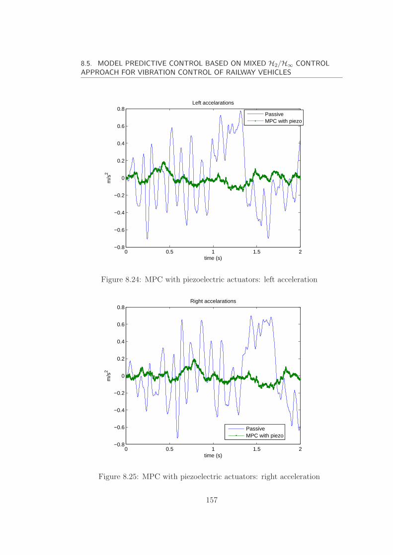
8.5. MODEL PREDICTIVE CONTROL BASED ON MIXED H2/H∞ CONTROLAPPROACH FOR VIBRATION CONTROL OF RAILWAY VEHICLES
0 0.5 1 1.5 2−0.8
−0.6
−0.4
−0.2
0
0.2
0.4
0.6
0.8
time (s)
m/s
2Left accelarations
PassiveMPC with piezo
Figure 8.24: MPC with piezoelectric actuators: left acceleration
0 0.5 1 1.5 2−0.8
−0.6
−0.4
−0.2
0
0.2
0.4
0.6
0.8
time (s)
m/s
2
Right accelarations
PassiveMPC with piezo
Figure 8.25: MPC with piezoelectric actuators: right acceleration
157
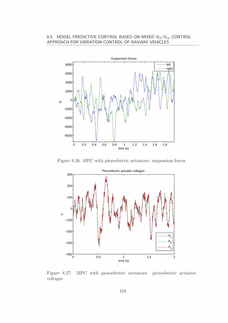
8.5. MODEL PREDICTIVE CONTROL BASED ON MIXED H2/H∞ CONTROLAPPROACH FOR VIBRATION CONTROL OF RAILWAY VEHICLES
0 0.2 0.4 0.6 0.8 1 1.2 1.4 1.6 1.8
−8000
−6000
−4000
−2000
0
2000
4000
6000
8000N
time (s)
Suspension forces
leftright
Figure 8.26: MPC with piezoelectric actuators: suspension forces
0 0.5 1 1.5 2−400
−300
−200
−100
0
100
200
300
V
time (s)
Piezoelectric actuator voltages
A1
A2
A3
Figure 8.27: MPC with piezoelectric actuators: piezoelectric actuatorvoltages
158
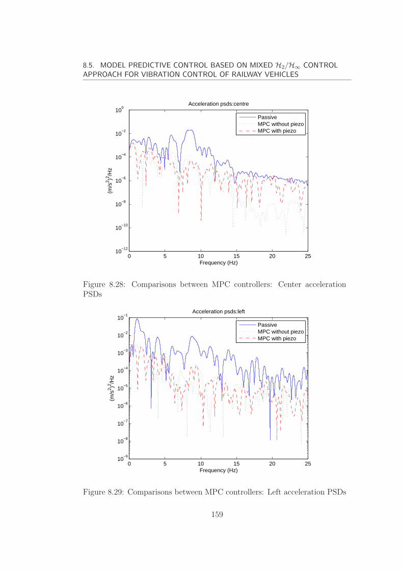
8.5. MODEL PREDICTIVE CONTROL BASED ON MIXED H2/H∞ CONTROLAPPROACH FOR VIBRATION CONTROL OF RAILWAY VEHICLES
0 5 10 15 20 2510
−12
10−10
10−8
10−6
10−4
10−2
100
Acceleration psds:centre
Frequency (Hz)
(m/s
2 )2 /Hz
PassiveMPC without piezoMPC with piezo
Figure 8.28: Comparisons between MPC controllers: Center accelerationPSDs
0 5 10 15 20 2510
−9
10−8
10−7
10−6
10−5
10−4
10−3
10−2
10−1
Acceleration psds:left
Frequency (Hz)
(m/s
2 )2 /Hz
PassiveMPC without piezoMPC with piezo
Figure 8.29: Comparisons between MPC controllers: Left acceleration PSDs
159
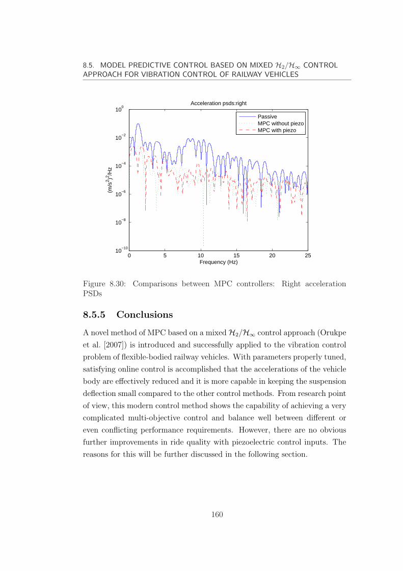
8.5. MODEL PREDICTIVE CONTROL BASED ON MIXED H2/H∞ CONTROLAPPROACH FOR VIBRATION CONTROL OF RAILWAY VEHICLES
0 5 10 15 20 2510
−10
10−8
10−6
10−4
10−2
100
Acceleration psds:right
Frequency (Hz)
(m/s
2 )2 /Hz
PassiveMPC without piezoMPC with piezo
Figure 8.30: Comparisons between MPC controllers: Right accelerationPSDs
8.5.5 Conclusions
A novel method of MPC based on a mixedH2/H∞ control approach (Orukpe
et al. [2007]) is introduced and successfully applied to the vibration control
problem of flexible-bodied railway vehicles. With parameters properly tuned,
satisfying online control is accomplished that the accelerations of the vehicle
body are effectively reduced and it is more capable in keeping the suspension
deflection small compared to the other control methods. From research point
of view, this modern control method shows the capability of achieving a very
complicated multi-objective control and balance well between different or
even conflicting performance requirements. However, there are no obvious
further improvements in ride quality with piezoelectric control inputs. The
reasons for this will be further discussed in the following section.
160
8.6. CONCLUDING REMARKS
8.6 Concluding remarks
This chapter has considered the design of centralized controllers for vibration
control of the flexible bodied railway vehicle. The full model that includes
rigid modes, flexible modes and the coupling terms between the rigid modes
and flexible modes is used as design model. Three control approaches
have been investigated:H2 optimal control, H∞ optimal control and model
predictive control based on a mixed H2/H∞ control approach.
In general, vibrations of the vehicle body have been effectively suppressed
with combined active suspension control and active structural damping with
piezoelectric actuators. It is found that the contribution of the piezoelectric
actuators in reducing the flexible modes can be limited. This may be due to
several reasons: 1) the full model is used for control design and modern
control methods are able to use full information of the system provided
by the design model; 2) active suspension controller designed with modern
methods in this case are effective in suppressing both the vertical rigid modes
and vertical bending modes, for there is a close connection between the
vertical rigid modes and vertical bending modes, which are the main flexible
mode portion of concern in this thesis. Piezoelectric actuators could be
complementary in reducing the effects of the flexible modes. Nevertheless,
the investigation in this chapter is a good preparation for future research
in vibration control of the railway vehicles when more flexible modes of the
vehicle body are taken into account.
161
Chapter 9
Conclusions and Future Work
9.1 Conclusions
Previous research on active secondary suspension has proved that it is an
effective way for vibration control of the railway vehicle to improve the ride
quality. However, its ability in suppressing the flexible modes is limited by
the dynamics of real actuators (e.g. hydraulic actuators) that are used for
suspension control and by the fact that the real vehicle body is complex
because it includes various flexible modes: vertical bending mode, horizontal
bending mode, torsional mode and diagonal distortion mode. Literature in
suppressing of the flexible modes of railway vehicles has been concentrated on
the application of piezoelectric actuators and sensors for structural damping
without including suspension control. Therefore, it is motivated to study
the combined control approach with both active suspension control and
active structural damping for improving the ride quality of the railway
vehicles. Active structural damping is realized by integrating piezoelectric
actuators and sensors onto the vehicle body together with appropriate control
strategies.
This thesis describes the modeling and control design for vibration
suppression of a typical flexible-bodied railway vehicle. The work is based
on a simplified side-view model of the railway vehicle with the vehicle body
assumed as a free-free beam. It is aimed to improve the vertical ride quality
162
9.1. CONCLUSIONS
of the railway vehicle. Hence bounce and pitch (rigid modes) of the vehicle
body and the vertical bending mode of the vehicle body are the modes of
concern for suppressing. The main contributions of this thesis are listed as
follows:
1. Rigorous modeling and related analysis of a flexible-bodied railway
vehicle with the so called smart structure, i.e. the vehicle body (assumed as
a free-free beam) integrated with piezoelectric actuators and sensors. The
modal analysis technique has been utilized for deriving the equations of
motion of the flexible modes and the derivation of couplings terms between
the rigid motion and flexible motion. The link between the rigid motion
and flexible motion suggests that it would be more effective to consider the
combined control of active suspension control and active structural damping.
2. The effect of flexibility of the vehicle body upon the ride quality is
investigated. Two controllers, i.e. modal controller with skyhook damping
and LQG controller, were designed using the rigid model as the design model.
The simulation of the closed-loop system with the controller that ignores the
flexibility in design stage shows degradation in ride quality which is caused
by flexibility of the vehicle body. So it is indicated that it is necessary to
introduce extra control for suppressing the flexibility of the vehicle body.
3. The procedure for placement of piezoelectric actuators and sensors
on the vehicle body with the application of the H2/ H∞ norms of flexible
structures(Gawronski [1998]) is presented. The candidate positions for
piezoelectric actuators and sensors are determined and four placement
configurations are chosen.
4. The investigation of two control strategies, i.e. decentralized control
and centralized control, for the combined active suspension control and active
structural damping with piezoelectric actuators.
With decentralized control, the couplings between the flexible motions
and the rigid motions are not taken into account during control design when
decoupled models are used for control design. In this case, the controller
for active suspension and the controller for structural damping are designed
independently for suppressing the rigid motion and the flexible motion
respectively. Two combinations of control methods have been investigated
163
9.1. CONCLUSIONS
: 1) modal control with skyhook damping for suspension control and LQG
control for structural damping with piezoelectric actuators and sensors. 2)
two individual LQG controllers for structural damping with piezoelectric
actuators and sensors and suspension control respectively. The damping
ratios of the flexible modes are effectively increased with the designed
controllers. The advanced control method achieves better ride quality than
classical control methods. The results show that the two sub controllers
are able to work in a complementary manner to each other in achieving a
satisfactory ride quality for the railway vehicle under consideration. When
the LQG controller for suspension control is designed with the full model, it
is shown that the contribution by the piezoelectric actuators is not evident
due to the fact that the suspension controller has already suppressed the first
bending flexible mode sufficiently.
5. With centralized control, the full model that includes rigid modes,
flexible modes and the coupling terms between the rigid modes and flexible
modes are used for control design. It presented the application of three
advanced control methods, i.e. H2 optimal control, H∞ optimal control and
model predictive control (MPC) based on a mixed H2/H∞ control approach
for designing the centralized controller.
Two H2 controllers have been designed with constant weights and with
frequency dependent weights respectively. The H2 controller with constant
weights achieves the lowest acceleration levels. When dynamic weights
are chosen to account for the limited bandwidth of hydraulic actuators
and to reflect the desired frequency range of the piezoelectric actuators, a
degradation is seen in the ride quality of the system. With piezoelectric
control included, its contribution in reducing the acceleration is not obvious,
however, it is seen that resonances in PSDs are eliminated, the flexibility of
the first flexible mode is further attenuated, and the control effort from the
actuators around the frequency of the first flexible mode is reduced. Then
the H∞ controller is designed via the signal based approach. Satisfactory
results have been obtained and improvements in ride quality are achieved
by including piezoelectric control inputs. Finally a novel method of MPC
164

9.2. SUGGESTIONS FOR FUTURE WORK
based on a mixed H2/H∞ control approach is investigated1. It has been
shown that the vibrations of the vehicle body are effectively suppressed with
this new method. However the improvement in ride quality provided by the
piezoelectric actuators is not evident.
The overall summary of the results is presented in Table 9.1. D1
represents the decentralized controller, K1 + Ksky, where K1 is the LQG
controller for active structural damping(with configuration 3) and Ksky is the
modal controller with skyhook damping for suspension control. D2 represents
the decentralized controller, K1 +KrLQG, where KrLQG is the LQG controller
designed with rigid model for suspension control.
In general, the advanced control approaches achieves better ride quality
than classical control approach. The H∞ controller is more conservative than
H2/LQG controllers in improving the ride quality while accomplish better
stability robustness. The MPC based on mixed H2/H∞ control approach
shows the capability of achieving multi-objective control that the level of
acceleration achieved is comparable to that achieved by H2 controller with
dynamic weights with better robustness properties in disturbance rejection.
Table 9.1: Percentage improvement in ride quality compared with the passivesystem
Strategy Center (%) Left (%) Right (%)D1 51.97 51.32 61.07D2 87.83 82.89 85.33H2 cons. weights 88.16 83.55 85.87H2 dyn. weights 85.20 78.62 82.13H∞ 81.25 77.96 83.47MPC 85.20 77.30 81.60
9.2 Suggestions for future work
The vehicle body was viewed as a free-free beam and only the vertical
bending modes were considered. In future research, more flexible modes
1This has been joint work between the author of the thesis and Dr. Orukpe,P.E (Orukpeet al. [2008])
165
9.2. SUGGESTIONS FOR FUTURE WORK
(e.g vertical bending mode, horizontal bending mode, torsional mode and
diagonal distortion mode) may be included in the vehicle model. This
will add to the complexity of the placement of the piezoelectric actuators
and sensors and the modeling of the flexible structure of the vehicle body
integrated with piezoelectric actuators and sensors and it is expected to see
that the piezoelectric actuators will possibly play a more important role in
active damping of the flexible structure.
Uncertainty was not included in the control design. Variations in values of
parameters such as of mass, damper and flexible frequency and mode shapes
will have an effect on the stability and performance of the system. Besides,
in theory, there is an infinite number of flexible modes, so the neglected
high-frequency modes may cause stability problems and degradation of
performance. Therefore, structured and unstructured uncertainties may be
introduced to the linear model in future control design. However, this will
yield a quite complex robust stability and robust performance problem as
well as larger scale models that may require a form of model reduction to
be performed. From the control design point of view, techniques such as
µ-synthesis may be employed to cater for worst case designs.
166

References
Mehdi Ahmadian and Andrew P. DeGuilio. Recent advances in the use
of piezoceramics for vibration suppression. The Shock and Vibration
Digest, 33(1), 2001.
Osama J. Aldraihem. Realistic determination of the optimal size and
location of piezoelectric actuator/sensors. Proceedings of the 1997 IEEE
International Conference on Control Application, Hartford,CT(October
5-7), 1997.
C. Benatzky, M. Kozek, and C. Bilik. Experimental control of a flexible
beam using a stack-bending actuator principle. Institute of Mechanics
and Mechatronics, Division of Control and Process Automation, Vienna
University of Technology.
Christian Benatzky and Martin Kozek. Influence of actuator size
and location on robust stability of actively controlled flexible beams.
Porceedings of the 17th World Congress The International Federation of
Automatic Control,Seoul,Korea, 2008.
Christian Benatzky, Martin Kozek, and Hanns Peter Jorgl. Comparison
of controller design methods for a scaled metro vehicle - flexible structure
experiment. Proceedings of the 2007 American Control Conference, New
York, USA, 2007.
R.E.D. Bishop and D.C. Johnson. The Mechanics of Vibration.
University Press Cambridge, Cambridge, UK, 1960.
167

REFERENCES
Chr Boller. State of the art and trends in using smart materials
and systems in transportation vehilces. Proceeding of Institution of
Mechanical Engineers, 212:149–158, 1998.
G. Capitani and M. Tibaldi. Reduced-order controllers for active
suspension of vehicles with flexible body. System Modelling and
Simulation, pages 201–206, 1989.
Inderjit Chopra. Review of state of art of smart structures and integrated
systems. AIAA Journal, 40(11):2145, 2002.
R.W. Clough and J. Penzien. Dynamics of Structures. McGraw-Hill,
New York, 1975.
B. Dumitrescu. Bounded real lemma for fir mimo systems. IEEE Signal
Process. Lett., 12(7), 2005.
D.J. Ewins. Modal Testing. 2nd edition, Research Studies Press, Baldock,
England, 2000.
E. Foo and R.M. Goodall. Active suspension control of flexible-bodied
railway vehicles using electro-hydraulic and electro-magnetic actuators.
Control Engineering Practice, 8:507–518, 2000.
Edwin Foo and R. M. Goodall. Active suspension control strategies for
flexible-bodied railway vehicles. UKACC International conference on
control ’ 98, pages 1300–1305, 1998.
T. H. E. Foo. Active Suspensions for Flexible-bodied Rail Vehicles. PhD
thesis, Loughborough University, Jun 2000.
Henri P. Gavin. Control of seismically excited vibration using
electrorheological materials and lyapunov methods. IEEE transaction
on control systems technology, 9(1), Jan 2001.
W. Gawronski. Advanced structural dynamics and active control of
structures. New York:Springer, 2004.
168
REFERENCES
W. Gawronski. Letters to the editor: simultaneous placement of
actuators and sensors. Journal of Sound and Vibration, 228(4):915–922,
1999.
Wodek K. Gawronski. Advanced Structural Dynamics and Active
Control of Structures. Springer, New York, 1998.
William B. Gevarter. Basic relations for control of flexible vehicles.
AIAA Journal, 8(4):666–672, April 1970.
R. M. Goodall. Active railway suspensions: Implementation status and
technological trends. Vehicle System Dynamics, 28(1997):87–117, 1997.
R. M. Goodall and W. Kortum. Mechatronic developments for railway
vehicles of the future. Control Engineering Practice, 10(8):887–898, 8
2002.
A. Hac. Stochastic optimal control of vehicles with elastic body and
active suspension. Journal of Dynamics Systems, Measurement and
Control, 108(2):106–110, 1986.
A. Hac. Suspension optimization of a 2-DOF vehicle model using a
stochastic optimal cotnrol technique. System Modelling and Simulation,
pages 201–206, 1989.
A. Hac and L. Liu. Sensor and actuator location in motion control of
flexible structures. Journal of Sound and Vibration, 167(2):239–261,
10/22 1993.
Aleksander Hac, Iijoong Youn, and Hsien H. Chen. Control of
suspensions for vehicles with flexible bodies-part I: Active suspensions.
Journal of Dynamic Systems, Measurement, and Control, 118:509–517,
1996a.
Aleksander Hac, Iijoong Youn, and Hsien H. Chen. Control of
suspensions for vehicles with flexible bodies-part II: Semi-active
suspensions. Journal of Dynamic Systems, Measurement, and Control,
118:519–525, 1996b.
169

REFERENCES
Duant Halim. Vibration analysis and control of smart structures. PhD
thesis, The University of Newcastle, New South Wales, Australia, 2002.
Dunant Halim and S.O. Reza Moheimani. Spatial h2 control of a
piezoelectric laminate beam: experimental implementation. IEEE
transactions on control systems technology, 10(4), 2002.
Dunant Halim and S.O. Reza Moheimani. Spatial resonant control of
flexible structures - application to a piezoelectric laminate beam. IEEE
transactions on control systems technology, 9(1), 2001.
J. Hansson, M. Takano, T. Takigami, Tomioka, and Y.Suzuki. Vibration
suppression of railway vehicle carbody with piezoelectric elements (a
study by using a scale model). JSME International Journal Series C.,
47(2), 2003.
S. Hurlebaus and L. Gaul. Smart structure dynamics. Mechanical
Systems and Signal Proceeding, 2005.
W.B. Spillman Jr, J.S. Sirkis, and P.T. Gardiner. Smart materials and
structures: what are they? Smart Materials and Structures, (5):247–
254, 1996.
Marke Kallio, Tatu Muukkonen, Seija Hietanen, Ismo Vessonen, Kari
Tammi, and Mikko Lehtonen. Smart Materials and Structures : VTT
research program 2000-2002. VTT Technical research centre of Finland,
Vuorimiehentie, Finland, 2002.
Takayoshi Kamada, Takayuki Tohtake, Tetsuro Aiba, and Masao Nagai.
Active vibration control of the railway vehicles by smart structure
concept. Proceedings of International Symposium on Speed-up and
Service Technology for Railway and Maglev Systems, 2005.
Takayoshi Kamada, Ryohei Kiuchi, and Masao Nagai. Suppression of
railway vehicle vibration by shunt damping using stack type piezoelectric
transducers. Vehicle System Dynamics, 46(Supplement):561–570, 2008.
170
REFERENCES
D.C. Karnopp. Are active suspension really necessary. The American
Society of Mechanical Engineers Winter Meeting(San Francisco), Paper
78-WA/DE-12, 1978.
D.C. Karnopp. Active and semi-active vibration control. Technical
report, Department of Mechnical and Aeronautical Engineering,
University of California, 1974.
Martin Kozek, Christian Benatzky, Alexander Schirrer, and An-
tonStribersky. Vibration damping of a flexible car body struc-
ture using piezo-stack actuators. Control Engineering Prac-
tice,doi:10.1016/j.conengprac.2009.08.001, 2009.
WW Law, WH Liao, and Huang. Vibration control of structures with
self-sensing piezoelectric actuators incorporating adaptive mechanisms.
Smart Materials and Structures, 12(5), 2003.
S. Leleu, H. Abou-Kandil, and Y. Bonnasieux. Piezoelectric actuators
and sensors location for active control of flexible structures. IEEE
transactions on Instrumentation and Measurement, 50(6):1577–1582,
2001.
H. Li and R. M. Goodall. Linear and non-linear skyhook damping control
laws for active railway suspensions. Control Engineering Practice, 7(7):
843–850, 1999.
S.O. Reza Moheimani. Resonant contol of structural vibration using
charge-driven piezoelectric actuators. IEEE transactions on control
systems technology, 13(6), 2005.
S.O. Reza Moheimani. A survey of recent innovations in vibration
damping and control using shunted piezoelectric transducers. IEEE
transactions on control systems technology, 11(4), 2003.
N. Nagai and Y. Sawada. Active suspension for flexible structure control
of high speed ground vehicles. In 10th World Congress on Automatic
Control, pages 197–202, 1987.
171
REFERENCES
Patience E. Orukpe, Xiang Zheng, I.M. Jaimoukha, A.C. Zolotas,
and R.M. Goodall. Model predictive control based on mixed control
approach for active vibration control of railway vehicles. Vehicle System
Dynamics, 46(1):151–160, 2008.
P.E. Orukpe, I.M. Jaimoukha, and H.M.H. El-Zobaidi. Model predictive
control based on mixed 〈2/〈∞ control approach. Proceedings of American
Control Conference, New York, USA, pages 6147–6150, 2007.
Anneli Orvnas. Methods for reducing vertical carbody vibrations of a
rail vehicle: A literature survey. KTH Engineering Sciences,Sweden,
2010.
Anneli Orvnas. Active secondary suspension in trains: A literature
survey of concepts and previous work. Royal Institutue of Technology,
Stockholm, 2008. ISBN 978-91-7415-144-2.
J.E. Paddison. Advance Control Strategies For Maglev Suspension
Systems. PhD thesis, Loughborough University, 1995.
S. Popprath, C. Benatzky, C. Bilki, M. Kozek, A. Stribersky, and
J. Wassermann. Experimental modal analysis of a scaled car body for
metro vehicles. The Thirteenth International Congress on Sound and
Vibration,Vienna,Austria, July 2006.
I. Pratt. Active Suspensions Applied to Railway Trains. PhD thesis,
Loughborough University, UK, 1996.
L.R. Ray. Robust linear-optimal control laws for active suspension
systems. Transactions of ASME, Journal of Dynamic Systems,
Measurement, and Control, 114(4):592–598, 1992.
Y.M. Sam and K.Hudha. Modelling and force tracking control of
hydrauic actuator for an active suspension system. IEEE, 2006.
Gerhard Schandl, Peter Lugner, Christian Benatzky, Martin Kozek,
and Anton Stribersky. Comfort enhancement by an active vibration
172
REFERENCES
reduction system for a flexible railway car body. Vehicle System
Dynamics, 45(9), 2007.
C. Scherer and S. Weiland. Linear matrix inequalities in control. DISC
course lecture notes, 2000.
A. Schirrer and M. Kozek. Co-simulation as effective method for flexible
structure vibration control. 16th Mediterranean Conference on Control
and Automation, Ajaccio, France, 2008.
Sigurd Skogestad and Ian Postletwaite. Multivarilable Feedback Control:
Analysis and design. John Wiley & Sons,Ltd., 2005.
Yoshiki Sugahara, Tadao Takigami, and Mitsuji Sampei. Suppressing
vertical vibration in railway vehicles through primary suspension
damping force control. Journal of System Design and Dynamics, 1(2),
2007.
Tadao Takigami and Takahiro Tomioka. Investigation to suppress
bending vibration of railway vehicle carbodies using piezoelectric
elements. QR of RTRI, 46(4), 2005.
Tadao Takigami and Takahiro Tomioka. Bending vibration suppression
of railway vehicle carbody with piezoelectric elements(experimental
results of excitation tests with a commuter car). Journal of Mechanical
Systems for Transportation and Logistics, 1(1), 2008.
Takayuki Tohtake, Masao Nagai, Takayoshi Kamada, and Hidehisa
Yoshida. Active vibration control of the railway vehicles by smart
structure. Proceedings of International Symposium on Speed-up and
Service Technology for Railway and Maglev Systems, 2005.
H. Tsunashima and S. Morichika. Ride quality improvement of agt
vehicle by active secondary suspension. Vehicle System Dynamics
Supplement, 41:764–773, 2004.
173
REFERENCES
H.S. Tzou and J.J. Hollkamp. Collocated independent modal
control with self-sensing orthogonal piezoelectric actuators(theory and
experiment. Smart Materials and Structures, 3(1994), 1994.
R. A. Williams. Comparison of Classical and Optimal Active Suspension
Control System. PhD thesis, Loughborough University, 1986.
P. Wu, J. Zeng, and H. Dai. Dynamic responses analysis of
railway passenger car with flexible carbody model based on semi-active
suspensions. Vehicle System Dynamics Supplement, 41:774–783, 2004.
Hazlina Md Yusof, Roger M. Goodall, and Roger Dixon. Controller
strategies for active secondary suspension actuators. IAVSD, 2011.
174

Appendices
175
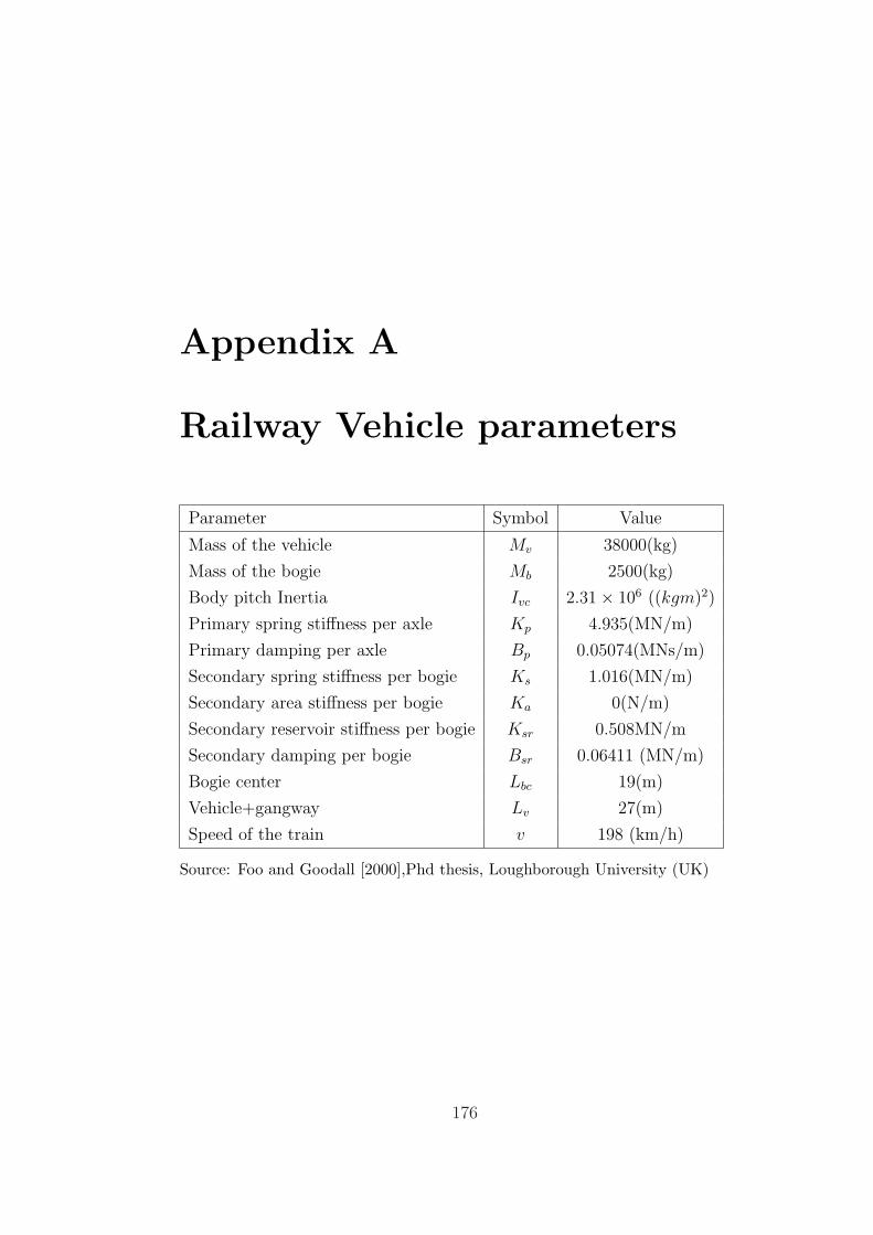
Appendix A
Railway Vehicle parameters
Parameter Symbol Value
Mass of the vehicle Mv 38000(kg)
Mass of the bogie Mb 2500(kg)
Body pitch Inertia Ivc 2.31× 10⁶ ((kgm)2)
Primary spring stiffness per axle Kp 4.935(MN/m)
Primary damping per axle Bp 0.05074(MNs/m)
Secondary spring stiffness per bogie Ks 1.016(MN/m)
Secondary area stiffness per bogie Ka 0(N/m)
Secondary reservoir stiffness per bogie Ksr 0.508MN/m
Secondary damping per bogie Bsr 0.06411 (MN/m)
Bogie center Lbc 19(m)
Vehicle+gangway Lv 27(m)
Speed of the train v 198 (km/h)
Source: Foo and Goodall [2000],Phd thesis, Loughborough University (UK)
176
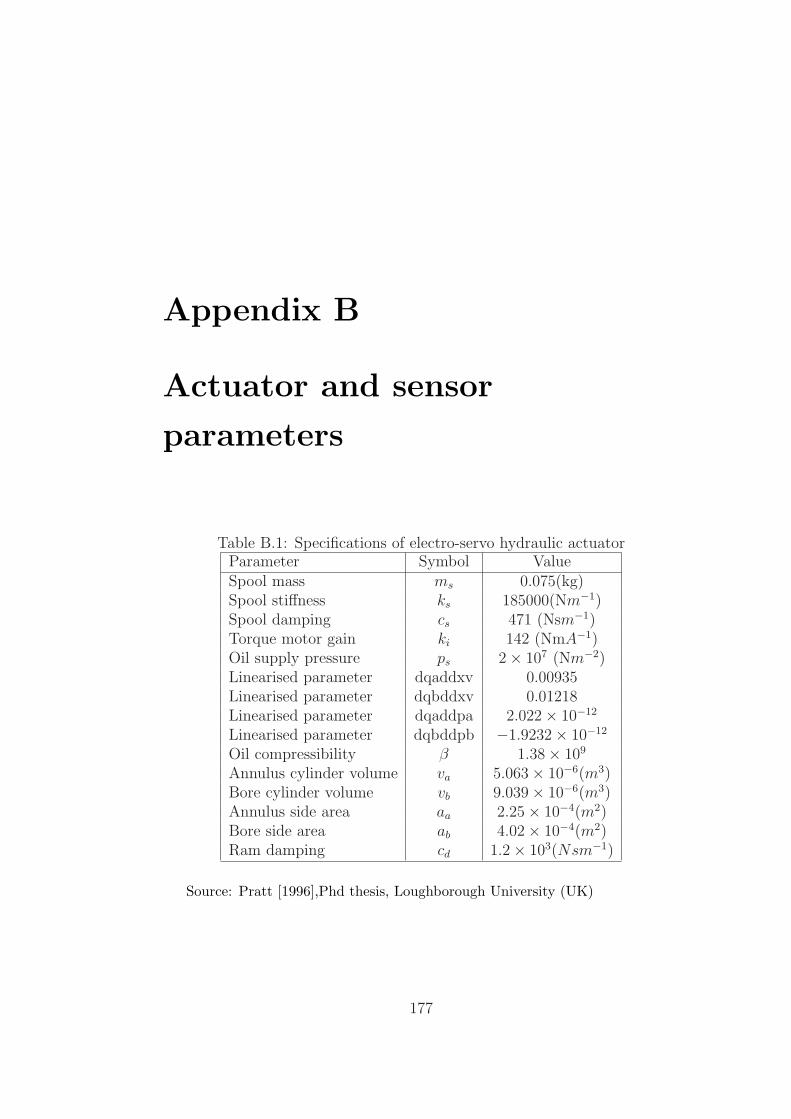
Appendix B
Actuator and sensor
parameters
Table B.1: Specifications of electro-servo hydraulic actuatorParameter Symbol ValueSpool mass ms 0.075(kg)Spool stiffness ks 185000(Nm−1)Spool damping cs 471 (Nsm−1)Torque motor gain ki 142 (NmA−1)Oil supply pressure ps 2× 10⁷ (Nm−2)Linearised parameter dqaddxv 0.00935Linearised parameter dqbddxv 0.01218Linearised parameter dqaddpa 2.022× 10⁻¹²
Linearised parameter dqbddpb −1.9232× 10⁻¹²
Oil compressibility β 1.38× 10⁹
Annulus cylinder volume va 5.063× 10⁻⁶(m3)Bore cylinder volume vb 9.039× 10⁻⁶(m3)Annulus side area aa 2.25× 10⁻⁴(m2)Bore side area ab 4.02× 10⁻⁴(m2)Ram damping cd 1.2× 10³(Nsm−1)
Source: Pratt [1996],Phd thesis, Loughborough University (UK)
177
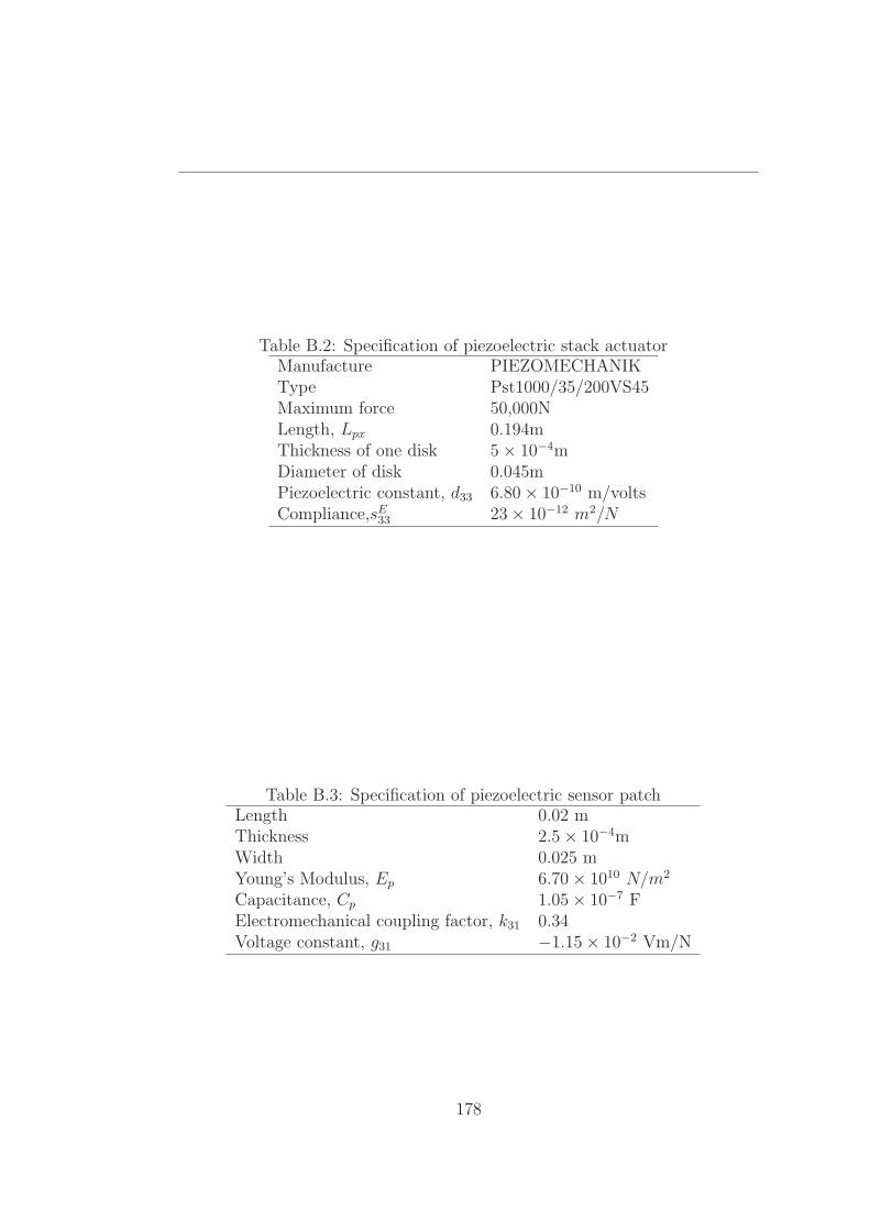
Table B.2: Specification of piezoelectric stack actuatorManufacture PIEZOMECHANIKType Pst1000/35/200VS45Maximum force 50,000NLength, Lpx 0.194mThickness of one disk 5× 10⁻⁴mDiameter of disk 0.045mPiezoelectric constant, d33 6.80× 10⁻¹⁰ m/voltsCompliance,sE
33 23× 10−12 m2/N
Table B.3: Specification of piezoelectric sensor patchLength 0.02 mThickness 2.5× 10⁻⁴mWidth 0.025 mYoung’s Modulus, Ep 6.70× 10¹⁰ N/m2
Capacitance, Cp 1.05× 10⁻⁷ FElectromechanical coupling factor, k31 0.34Voltage constant, g31 −1.15× 10⁻² Vm/N
178
Appendix C
Publications of research work
[1] Patience E. Orukpe, X.Zheng, I.M.Jaimoukha, A.C.Zolotas and R.M.Goodall
Model predictive control based on mixed control approach for active vibration
control of railway vehicles Vehicle System Dynamics, 46:1, 151-160,2008
[2] X.Zheng and A.C.Zolotas and R.M.Goodall Modeling of flexible-bodied railway
vehicles for vibration suppression ICSE, Coventry, UK, Sep 2006
[3]X.Zheng and A.C.Zolotas and H.Wang. Mathematica implementation of output-
feedback pole assignment for uncertain systems via symbolic algebra International
Journal of Control, Vol. 79, No.11, 1431-1446, Nov 2006
179