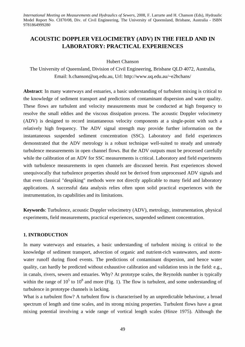
International Meeting on Measurements and Hydraulics of Sewers, 2008, F. Larrarte and H. Chanson (Eds), Hydraulic Model Report No. CH70/08, Div. of Civil Engineering, The University of Queensland, Brisbane, Australia - ISBN 9781864999280

49

ACOUSTIC DOPPLER VELOCIMETRY (ADV) IN THE FIELD AND IN

LABORATORY: PRACTICAL EXPERIENCES

Hubert Chanson The University of Queensland, Division of Civil Engineering, Brisbane QLD 4072, Australia,

Email: h.chanson@uq.edu.au, Url: http://www.uq.edu.au/~e2hchans/ Abstract: In many waterways and estuaries, a basic understanding of turbulent mixing is critical to the knowledge of sediment transport and predictions of contaminant dispersion and water quality. These flows are turbulent and velocity measurements must be conducted at high frequency to resolve the small eddies and the viscous dissipation process. The acoustic Doppler velocimetry (ADV) is designed to record instantaneous velocity components at a single-point with such a relatively high frequency. The ADV signal strength may provide further information on the instantaneous suspended sediment concentration (SSC). Laboratory and field experiences demonstrated that the ADV metrology is a robust technique well-suited to steady and unsteady turbulence measurements in open channel flows. But the ADV outputs must be processed carefully while the calibration of an ADV for SSC measurements is critical. Laboratory and field experiments with turbulence measurements in open channels are discussed herein. Past experiences showed unequivocally that turbulence properties should not be derived from unprocessed ADV signals and that even classical "despiking" methods were not directly applicable to many field and laboratory applications. A successful data analysis relies often upon solid practical experiences with the instrumentation, its capabilities and its limitations. Keywords: Turbulence, acoustic Doppler velocimetry (ADV), metrology, instrumentation, physical experiments, field measurements, practical experiences, suspended sediment concentration.

1. INTRODUCTION

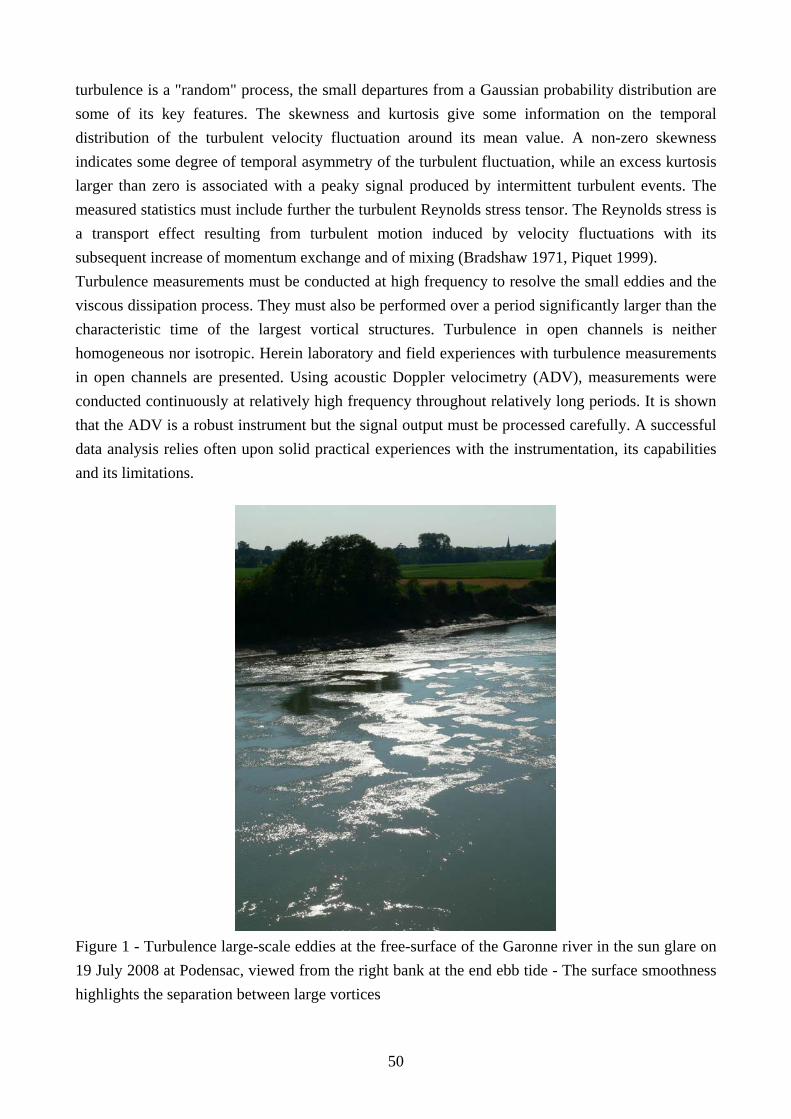
In many waterways and estuaries, a basic understanding of turbulent mixing is critical to the knowledge of sediment transport, advection of organic and nutrient-rich wastewaters, and storm-water runoff during flood events. The predictions of contaminant dispersion, and hence water quality, can hardly be predicted without exhaustive calibration and validation tests in the field: e.g., in canals, rivers, sewers and estuaries. Why? At prototype scales, the Reynolds number is typically within the range of 105 to 108 and more (Fig. 1). The flow is turbulent, and some understanding of turbulence in prototype channels is lacking. What is a turbulent flow? A turbulent flow is characterised by an unpredictable behaviour, a broad spectrum of length and time scales, and its strong mixing properties. Turbulent flows have a great mixing potential involving a wide range of vortical length scales (Hinze 1975). Although the

50

turbulence is a "random" process, the small departures from a Gaussian probability distribution are some of its key features. The skewness and kurtosis give some information on the temporal distribution of the turbulent velocity fluctuation around its mean value. A non-zero skewness indicates some degree of temporal asymmetry of the turbulent fluctuation, while an excess kurtosis larger than zero is associated with a peaky signal produced by intermittent turbulent events. The measured statistics must include further the turbulent Reynolds stress tensor. The Reynolds stress is a transport effect resulting from turbulent motion induced by velocity fluctuations with its subsequent increase of momentum exchange and of mixing (Bradshaw 1971, Piquet 1999). Turbulence measurements must be conducted at high frequency to resolve the small eddies and the viscous dissipation process. They must also be performed over a period significantly larger than the characteristic time of the largest vortical structures. Turbulence in open channels is neither homogeneous nor isotropic. Herein laboratory and field experiences with turbulence measurements in open channels are presented. Using acoustic Doppler velocimetry (ADV), measurements were conducted continuously at relatively high frequency throughout relatively long periods. It is shown that the ADV is a robust instrument but the signal output must be processed carefully. A successful data analysis relies often upon solid practical experiences with the instrumentation, its capabilities and its limitations.

Figure 1 - Turbulence large-scale eddies at the free-surface of the Garonne river in the sun glare on 19 July 2008 at Podensac, viewed from the right bank at the end ebb tide - The surface smoothness highlights the separation between large vortices

51

2. TURBULENT VELOCITY MEASUREMENTS WITH ACOUSTIC DOPPLER VELOCIMETER

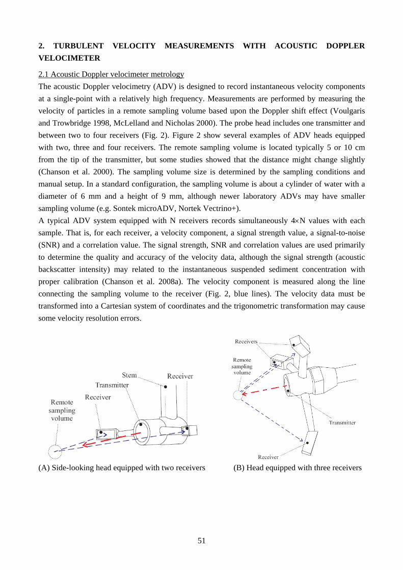
2.1 Acoustic Doppler velocimeter metrology The acoustic Doppler velocimetry (ADV) is designed to record instantaneous velocity components at a single-point with a relatively high frequency. Measurements are performed by measuring the velocity of particles in a remote sampling volume based upon the Doppler shift effect (Voulgaris and Trowbridge 1998, McLelland and Nicholas 2000). The probe head includes one transmitter and between two to four receivers (Fig. 2). Figure 2 show several examples of ADV heads equipped with two, three and four receivers. The remote sampling volume is located typically 5 or 10 cm from the tip of the transmitter, but some studies showed that the distance might change slightly (Chanson et al. 2000). The sampling volume size is determined by the sampling conditions and manual setup. In a standard configuration, the sampling volume is about a cylinder of water with a diameter of 6 mm and a height of 9 mm, although newer laboratory ADVs may have smaller sampling volume (e.g. Sontek microADV, Nortek Vectrino+). A typical ADV system equipped with N receivers records simultaneously 4×N values with each sample. That is, for each receiver, a velocity component, a signal strength value, a signal-to-noise (SNR) and a correlation value. The signal strength, SNR and correlation values are used primarily to determine the quality and accuracy of the velocity data, although the signal strength (acoustic backscatter intensity) may related to the instantaneous suspended sediment concentration with proper calibration (Chanson et al. 2008a). The velocity component is measured along the line connecting the sampling volume to the receiver (Fig. 2, blue lines). The velocity data must be transformed into a Cartesian system of coordinates and the trigonometric transformation may cause some velocity resolution errors.

(A) Side-looking head equipped with two receivers (B) Head equipped with three receivers

52

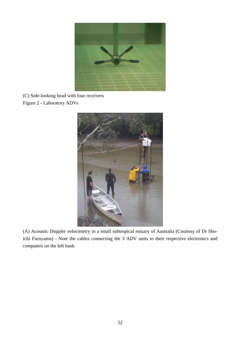
(C) Side-looking head with four receivers Figure 2 - Laboratory ADVs

(A) Acoustic Doppler velocimetry in a small subtropical estuary of Australia (Courtesy of Dr Sho-ichi Furuyama) - Note the cables connecting the 3 ADV units to their respective electronics and computers on the left bank

53

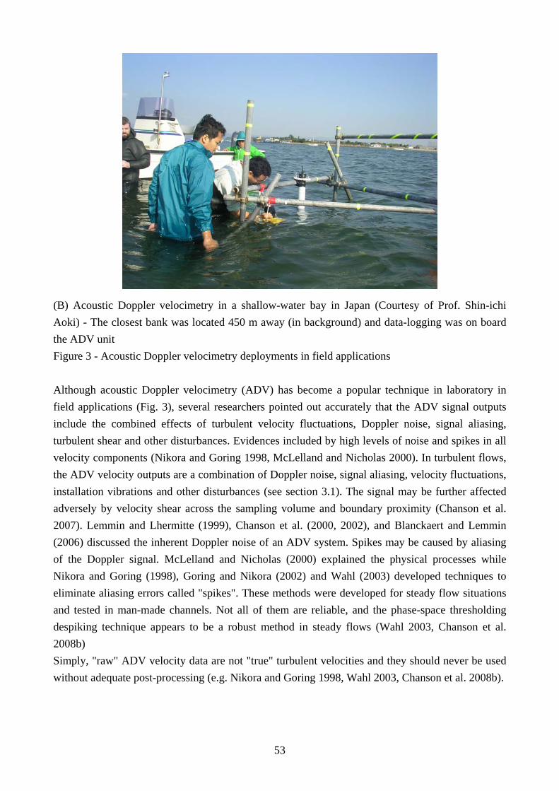
(B) Acoustic Doppler velocimetry in a shallow-water bay in Japan (Courtesy of Prof. Shin-ichi Aoki) - The closest bank was located 450 m away (in background) and data-logging was on board the ADV unit Figure 3 - Acoustic Doppler velocimetry deployments in field applications Although acoustic Doppler velocimetry (ADV) has become a popular technique in laboratory in field applications (Fig. 3), several researchers pointed out accurately that the ADV signal outputs include the combined effects of turbulent velocity fluctuations, Doppler noise, signal aliasing, turbulent shear and other disturbances. Evidences included by high levels of noise and spikes in all velocity components (Nikora and Goring 1998, McLelland and Nicholas 2000). In turbulent flows, the ADV velocity outputs are a combination of Doppler noise, signal aliasing, velocity fluctuations, installation vibrations and other disturbances (see section 3.1). The signal may be further affected adversely by velocity shear across the sampling volume and boundary proximity (Chanson et al. 2007). Lemmin and Lhermitte (1999), Chanson et al. (2000, 2002), and Blanckaert and Lemmin (2006) discussed the inherent Doppler noise of an ADV system. Spikes may be caused by aliasing of the Doppler signal. McLelland and Nicholas (2000) explained the physical processes while Nikora and Goring (1998), Goring and Nikora (2002) and Wahl (2003) developed techniques to eliminate aliasing errors called "spikes". These methods were developed for steady flow situations and tested in man-made channels. Not all of them are reliable, and the phase-space thresholding despiking technique appears to be a robust method in steady flows (Wahl 2003, Chanson et al. 2008b) Simply, "raw" ADV velocity data are not "true" turbulent velocities and they should never be used without adequate post-processing (e.g. Nikora and Goring 1998, Wahl 2003, Chanson et al. 2008b).

54

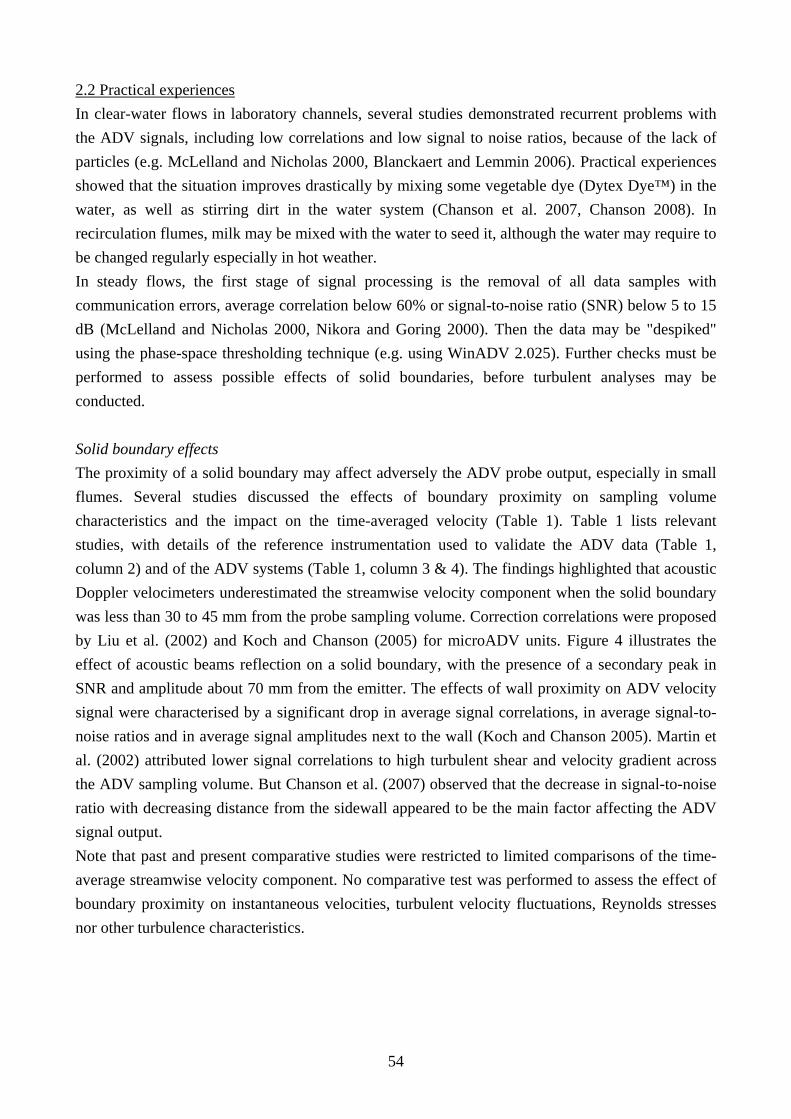
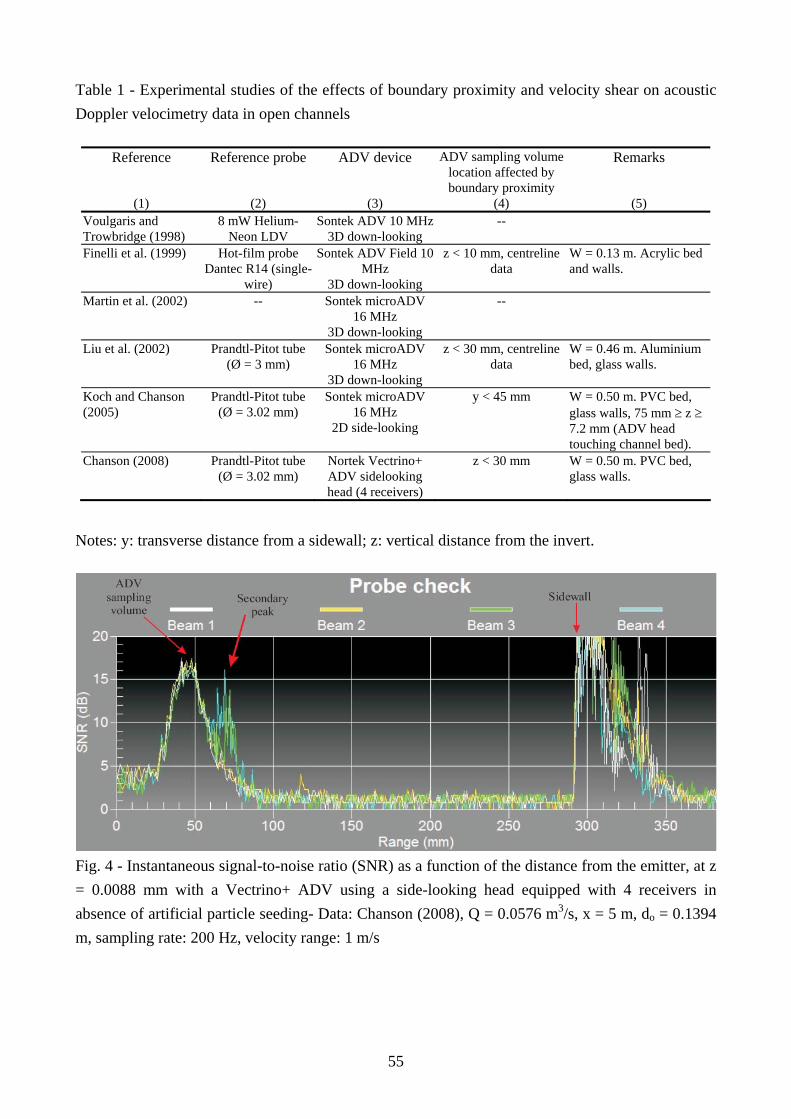
2.2 Practical experiences In clear-water flows in laboratory channels, several studies demonstrated recurrent problems with the ADV signals, including low correlations and low signal to noise ratios, because of the lack of particles (e.g. McLelland and Nicholas 2000, Blanckaert and Lemmin 2006). Practical experiences showed that the situation improves drastically by mixing some vegetable dye (Dytex Dye™) in the water, as well as stirring dirt in the water system (Chanson et al. 2007, Chanson 2008). In recirculation flumes, milk may be mixed with the water to seed it, although the water may require to be changed regularly especially in hot weather. In steady flows, the first stage of signal processing is the removal of all data samples with communication errors, average correlation below 60% or signal-to-noise ratio (SNR) below 5 to 15 dB (McLelland and Nicholas 2000, Nikora and Goring 2000). Then the data may be "despiked" using the phase-space thresholding technique (e.g. using WinADV 2.025). Further checks must be performed to assess possible effects of solid boundaries, before turbulent analyses may be conducted. Solid boundary effects The proximity of a solid boundary may affect adversely the ADV probe output, especially in small flumes. Several studies discussed the effects of boundary proximity on sampling volume characteristics and the impact on the time-averaged velocity (Table 1). Table 1 lists relevant studies, with details of the reference instrumentation used to validate the ADV data (Table 1, column 2) and of the ADV systems (Table 1, column 3 & 4). The findings highlighted that acoustic Doppler velocimeters underestimated the streamwise velocity component when the solid boundary was less than 30 to 45 mm from the probe sampling volume. Correction correlations were proposed by Liu et al. (2002) and Koch and Chanson (2005) for microADV units. Figure 4 illustrates the effect of acoustic beams reflection on a solid boundary, with the presence of a secondary peak in SNR and amplitude about 70 mm from the emitter. The effects of wall proximity on ADV velocity signal were characterised by a significant drop in average signal correlations, in average signal-to-noise ratios and in average signal amplitudes next to the wall (Koch and Chanson 2005). Martin et al. (2002) attributed lower signal correlations to high turbulent shear and velocity gradient across the ADV sampling volume. But Chanson et al. (2007) observed that the decrease in signal-to-noise ratio with decreasing distance from the sidewall appeared to be the main factor affecting the ADV signal output. Note that past and present comparative studies were restricted to limited comparisons of the time-average streamwise velocity component. No comparative test was performed to assess the effect of boundary proximity on instantaneous velocities, turbulent velocity fluctuations, Reynolds stresses nor other turbulence characteristics.

55

Table 1 - Experimental studies of the effects of boundary proximity and velocity shear on acoustic Doppler velocimetry data in open channels

Reference Reference probe ADV device ADV sampling volume location affected by boundary proximity

Remarks

(1) (2) (3) (4) (5) Voulgaris and Trowbridge (1998)

8 mW Helium-Neon LDV

Sontek ADV 10 MHz3D down-looking

--

Finelli et al. (1999) Hot-film probe Dantec R14 (single-

wire)

Sontek ADV Field 10 MHz

3D down-looking

z < 10 mm, centreline data

W = 0.13 m. Acrylic bed and walls.

Martin et al. (2002) -- Sontek microADV 16 MHz

3D down-looking

--

Liu et al. (2002) Prandtl-Pitot tube (Ø = 3 mm)

Sontek microADV 16 MHz

3D down-looking

z < 30 mm, centreline data

W = 0.46 m. Aluminium bed, glass walls.

Koch and Chanson (2005)

Prandtl-Pitot tube (Ø = 3.02 mm)

Sontek microADV 16 MHz

2D side-looking

y < 45 mm W = 0.50 m. PVC bed, glass walls, 75 mm ≥ z ≥ 7.2 mm (ADV head touching channel bed).

Chanson (2008) Prandtl-Pitot tube (Ø = 3.02 mm)

Nortek Vectrino+ ADV sidelooking head (4 receivers)

z < 30 mm W = 0.50 m. PVC bed, glass walls.

Notes: y: transverse distance from a sidewall; z: vertical distance from the invert.

Fig. 4 - Instantaneous signal-to-noise ratio (SNR) as a function of the distance from the emitter, at z = 0.0088 mm with a Vectrino+ ADV using a side-looking head equipped with 4 receivers in absence of artificial particle seeding- Data: Chanson (2008), Q = 0.0576 m3/s, x = 5 m, do = 0.1394 m, sampling rate: 200 Hz, velocity range: 1 m/s

56

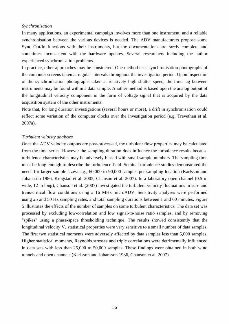
Synchronisation In many applications, an experimental campaign involves more than one instrument, and a reliable synchronisation between the various devices is needed. The ADV manufacturers propose some Sync Out/In functions with their instruments, but the documentations are rarely complete and sometimes inconsistent with the hardware updates. Several researchers including the author experienced synchronisation problems. In practice, other approaches may be considered. One method uses synchronisation photographs of the computer screens taken at regular intervals throughout the investigation period. Upon inspection of the synchronisation photographs taken at relatively high shutter speed, the time lag between instruments may be found within a data sample. Another method is based upon the analog output of the longitudinal velocity component in the form of voltage signal that is acquired by the data acquisition system of the other instruments. Note that, for long duration investigations (several hours or more), a drift in synchronisation could reflect some variation of the computer clocks over the investigation period (e.g. Trevethan et al. 2007a). Turbulent velocity analyses Once the ADV velocity outputs are post-processed, the turbulent flow properties may be calculated from the time series. However the sampling duration does influence the turbulence results because turbulence characteristics may be adversely biased with small sample numbers. The sampling time must be long enough to describe the turbulence field. Seminal turbulence studies demonstrated the needs for larger sample sizes: e.g., 60,000 to 90,000 samples per sampling location (Karlsson and Johansson 1986, Krogstad et al. 2005, Chanson et al. 2007). In a laboratory open channel (0.5 m wide, 12 m long), Chanson et al. (2007) investigated the turbulent velocity fluctuations in sub- and trans-critical flow conditions using a 16 MHz microADV. Sensitivity analyses were performed using 25 and 50 Hz sampling rates, and total sampling durations between 1 and 60 minutes. Figure 5 illustrates the effects of the number of samples on some turbulent characteristics. The data set was processed by excluding low-correlation and low signal-to-noise ratio samples, and by removing "spikes" using a phase-space thresholding technique. The results showed consistently that the longitudinal velocity Vx statistical properties were very sensitive to a small number of data samples. The first two statistical moments were adversely affected by data samples less than 5,000 samples. Higher statistical moments, Reynolds stresses and triple correlations were detrimentally influenced in data sets with less than 25,000 to 50,000 samples. These findings were obtained in both wind tunnels and open channels (Karlsson and Johansson 1986, Chanson et al. 2007).

57

-0.1

-0.08

-0.06

-0.04

-0.02

0

0.02

0.04

1000 10000 100000 1000000-3

-2

-1

0

1

2

3

4

Error on Std(Vx)Error on Kurtosis(Vx)

Nb of samples

Error on Std(Vx) Error on Kurtosis(Vx)

Fig. 5 - Effects of data sample size on turbulence characteristics in open channel flow: error on longitudinal velocity standard deviation and kurtosis - Data: Chanson et al. (2007), Q = 0.0404 m3/s, W = 0.5 m, d = 0.096 m, z = 27.2 mm, microADV (16 MHz) with 2D side-looking head, sampling rate: 50 Hz, velocity range: 1 m/s Unsteady turbulence The ADV signal processing and velocity analysis must be adapted in unsteady flows. While several post-processing techniques were devised for steady flows, these are not applicable to unsteady flow situations (e.g. Nikora 2004, Person. Comm.). In tidal bore flows, Koch and Chanson (2008) and Chanson (2008) used a post-processing limited to the removal of communication errors, and the turbulent properties were calculated using a variable-interval time average (VITA) method. The instantaneous turbulent velocity v was decomposed as: v = V - V , where V is the instantaneous velocity and V is a low-pass filtered velocity component, or variable-interval time average (Piquet 1999, Koch and Chanson 2005). With this method, the cutoff frequency must be selected such that the averaging time is greater than the characteristic period of fluctuations, and small with respect to the characteristic period for the time-evolution of the mean properties (Koch and Chanson 2005,2008, Garcia and Garcia 2006, Chanson 2008). Its selection is based upon a detailed sensitivity analysis as illustrated by Koch and Chanson (2005,2008). Turbulent properties including the Reynolds stress tensor are then calculated from the high-pass filtered signals.

3. TURBULENT VELOCITY MEASUREMENTS: FIELD EXPERIENCE

3.1 Presentation Recent studies of turbulence in estuarine systems highlighted that the field measurements must be conducted over long-durations at high-frequency (25 to 50 Hz): e.g., 25 to 50 hours in a small estuary (Chanson et al. 2005, Trevethan et al. 2007a,b,2008). Extensive ADV measurements in a small estuary provided some practical knowledge, and showed conclusively that the turbulence properties could not be derived from unprocessed ADV signals and that even "classical" despiking methods were not directly applicable to unsteady estuary flows (Chanson et al. 2008a).

58

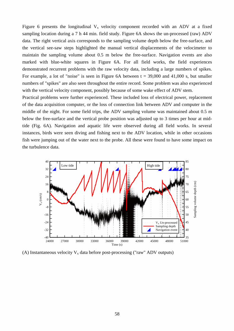
Figure 6 presents the longitudinal Vx velocity component recorded with an ADV at a fixed sampling location during a 7 h 44 min. field study. Figure 6A shows the un-processed (raw) ADV data. The right vertical axis corresponds to the sampling volume depth below the free-surface, and the vertical see-saw steps highlighted the manual vertical displacements of the velocimeter to maintain the sampling volume about 0.5 m below the free-surface. Navigation events are also marked with blue-white squares in Figure 6A. For all field works, the field experiences demonstrated recurrent problems with the raw velocity data, including a large numbers of spikes. For example, a lot of "noise" is seen in Figure 6A between t = 39,000 and 41,000 s, but smaller numbers of "spikes" are also seen throughout the entire record. Some problem was also experienced with the vertical velocity component, possibly because of some wake effect of ADV stem. Practical problems were further experienced. These included loss of electrical power, replacement of the data acquisition computer, or the loss of connection link between ADV and computer in the middle of the night. For some field trips, the ADV sampling volume was maintained about 0.5 m below the free-surface and the vertical probe position was adjusted up to 3 times per hour at mid-tide (Fig. 6A). Navigation and aquatic life were observed during all field works. In several instances, birds were seen diving and fishing next to the ADV location, while in other occasions fish were jumping out of the water next to the probe. All these were found to have some impact on the turbulence data.

Time (s)

Vx (

cm/s

)

Sam

plin

g vo

lum

e de

pth

(cm

)

24000 27000 30000 33000 36000 39000 42000 45000 48000 51000-40 35

-32 40

-24 45

-16 50

-8 55

0 60

8 65

16 70

24 75

32 80

40 85High tideLow tide

Vx Un-processedSampling depthNavigation event

(A) Instantaneous velocity Vx data before post-processing ("raw" ADV outputs)

59

Time (s)

Vx (

cm/s

)

Sam

plin

g vo

lum

e de

pth

(cm

)

24000 27000 30000 33000 36000 39000 42000 45000 48000 51000-40 35

-32 40

-24 45

-16 50

-8 55

0 60

8 65

16 70

24 75

32 80

40 85High tideLow tide

Vx Post-processed

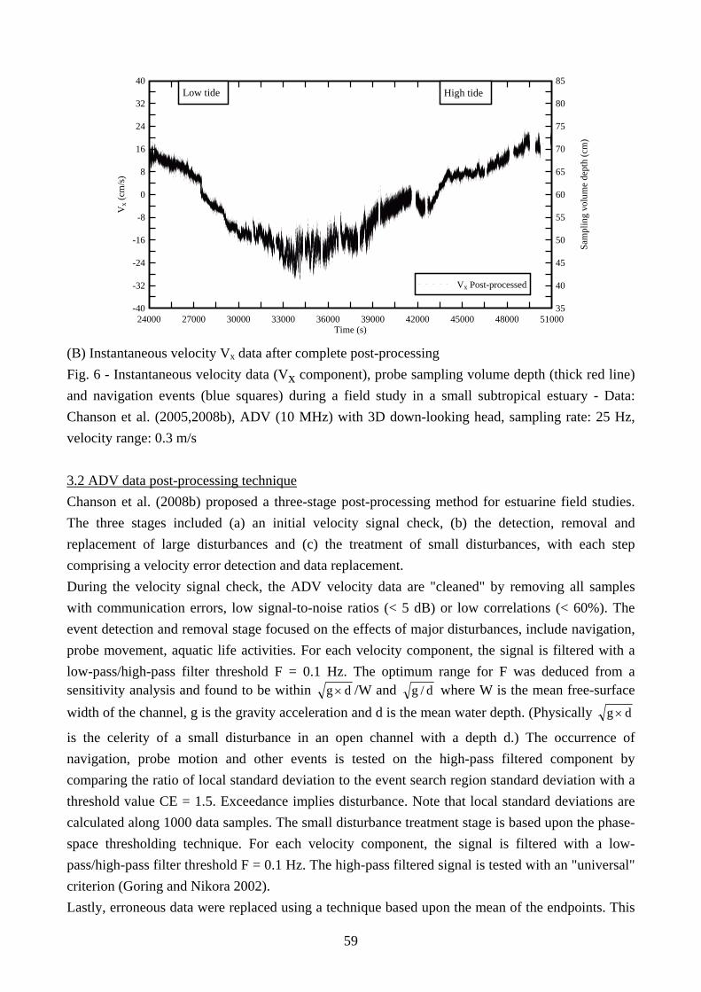
(B) Instantaneous velocity Vx data after complete post-processing Fig. 6 - Instantaneous velocity data (Vx component), probe sampling volume depth (thick red line) and navigation events (blue squares) during a field study in a small subtropical estuary - Data: Chanson et al. (2005,2008b), ADV (10 MHz) with 3D down-looking head, sampling rate: 25 Hz, velocity range: 0.3 m/s 3.2 ADV data post-processing technique Chanson et al. (2008b) proposed a three-stage post-processing method for estuarine field studies. The three stages included (a) an initial velocity signal check, (b) the detection, removal and replacement of large disturbances and (c) the treatment of small disturbances, with each step comprising a velocity error detection and data replacement. During the velocity signal check, the ADV velocity data are "cleaned" by removing all samples with communication errors, low signal-to-noise ratios (< 5 dB) or low correlations (< 60%). The event detection and removal stage focused on the effects of major disturbances, include navigation, probe movement, aquatic life activities. For each velocity component, the signal is filtered with a low-pass/high-pass filter threshold F = 0.1 Hz. The optimum range for F was deduced from a sensitivity analysis and found to be within dg × /W and d/g where W is the mean free-surface width of the channel, g is the gravity acceleration and d is the mean water depth. (Physically dg ×

is the celerity of a small disturbance in an open channel with a depth d.) The occurrence of navigation, probe motion and other events is tested on the high-pass filtered component by comparing the ratio of local standard deviation to the event search region standard deviation with a threshold value CE = 1.5. Exceedance implies disturbance. Note that local standard deviations are calculated along 1000 data samples. The small disturbance treatment stage is based upon the phase-space thresholding technique. For each velocity component, the signal is filtered with a low-pass/high-pass filter threshold F = 0.1 Hz. The high-pass filtered signal is tested with an "universal" criterion (Goring and Nikora 2002). Lastly, erroneous data were replaced using a technique based upon the mean of the endpoints. This

60

technique reduced distortion of statistical values, while not inferring trends on the replaced data. Applications Extensive field experiences in Australia and Japan suggested that the turbulence properties could not be extrapolated from the unprocessed data sets during field works in estuaries (Trevethan 2008, Chanson et al. 2008b). Classical ADV despiking techniques were tested and the results demonstrated that "conventional" ADV despiking techniques were not suitable. Velocity fluctuations might be induced by large disturbances such as aquatic life, navigation, debris and experimental procedure. Even in optimum conditions, natural estuarine systems, and even sewer systems, are characterised by unsteady flows, and the hydrodynamics cannot be assumed to be quasi-steady over a statistically-meaningful data sample. The ADV post-processing method was tested extensively with a dozen of long duration field studies in Australia and Japan. Figure 6B illustrates the outcomes of ADV data post-processing for a field study. It may be compared with the un-processed data set (Fig. 6A). The comparison shows the successful detection and removal of all major disturbances and of a lot of spikes and noise (e.g. 38,000 < t < 41,000 s). Using the above ADV post-processing method, between 10 to 25% of all samples were removed and replaced. Such quantities are fairly significant and do impact onto the turbulent flow properties. A systematic comparison between "raw" and post-processed ADV data demonstrated that all turbulence characteristics were affected by the post-processing. All turbulent properties, including the time-average velocities, were improperly estimated from un-processed data sets.

4. SUSPENDED SEDIMENT CONCENTRATION MEASUREMENTS

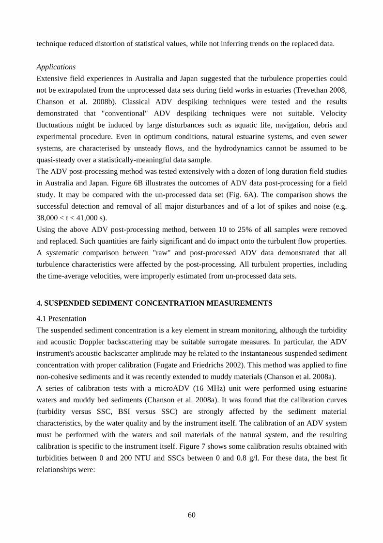
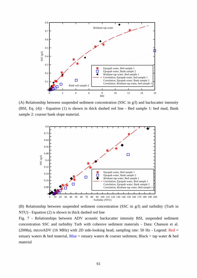
4.1 Presentation The suspended sediment concentration is a key element in stream monitoring, although the turbidity and acoustic Doppler backscattering may be suitable surrogate measures. In particular, the ADV instrument's acoustic backscatter amplitude may be related to the instantaneous suspended sediment concentration with proper calibration (Fugate and Friedrichs 2002). This method was applied to fine non-cohesive sediments and it was recently extended to muddy materials (Chanson et al. 2008a). A series of calibration tests with a microADV (16 MHz) unit were performed using estuarine waters and muddy bed sediments (Chanson et al. 2008a). It was found that the calibration curves (turbidity versus SSC, BSI versus SSC) are strongly affected by the sediment material characteristics, by the water quality and by the instrument itself. The calibration of an ADV system must be performed with the waters and soil materials of the natural system, and the resulting calibration is specific to the instrument itself. Figure 7 shows some calibration results obtained with turbidities between 0 and 200 NTU and SSCs between 0 and 0.8 g/l. For these data, the best fit relationships were:

61

BSI

SSC

(g/l)

0 2 4 6 8 10 12 14 160

0.1

0.2

0.3

0.4

0.5

0.6

0.7

0.8

Brisbane tap water

Bank soil sample 2

Eprapah water, Bed sample 1Eprapah water, Bank sample 2Brisbane tap water, Bed sample 1Correlation, Eprapah water, bed sample 1Correlation, Eprapah water, Bank sample 2Correlation, Brisbane tap water, bed sample 1

(A) Relationship between suspended sediment concentration (SSC in g/l) and backscatter intensity (BSI, Eq. (4)) - Equation (1) is shown in thick dashed red line - Bed sample 1: bed mud, Bank sample 2: coarser bank slope material.

Turbidity (NTU)

SSC

(g/l)

0 10 20 30 40 50 60 70 80 90 100 110 120 130 140 150 160 170 180 190 2000

0.08

0.16

0.24

0.32

0.4

0.48

0.56

0.64

0.72

0.8

Eprapah water, Bed sample 1Eprapah water, Bank sample 2Brisbane tap water, Bed sample 1Correlation, Eprapah water, Bed sample 1Correlation, Eprapah water, Bank sample 2Correlation, Brisbane tap water, Bed sample 1

(B) Relationship between suspended sediment concentration (SSC in g/l) and turbidity (Turb in NTU) - Equation (2) is shown in thick dashed red line Fig. 7 - Relationships between ADV acoustic backscatter intensity BSI, suspended sediment concentration SSC and turbidity Turb with cohesive sediment materials - Data: Chanson et al. (2008a), microADV (16 MHz) with 2D side-looking head, sampling rate: 50 Hz - Legend: Red = estuary waters & bed material, Blue = estuary waters & coarser sediment, Black = tap water & bed material

62

( )BSI1109.0e19426.0SSC ×−−×= (1)

0350.0Turb00485.0SSC −×= (2)

( )BSI1593.0e11.171Turb ×−−×= (3)

where SSC is in g/l, Turb is in NTU and the backscatter intensity BSI is defined as: Ampl043.05 1010BSI ×− ×= (4)

with Ampl the average signal amplitude data measured in counts by the ADV system. The coefficient 10-5 was a value introduced to avoid large values of BSI. 4.2 Application Using such a calibration, an ADV can record simultaneously the turbulent velocities and SSC in the same control volume at high-frequency. Field observations in Australia (Eprapah Creek) showed large SSC fluctuations throughout the entire field studies, including during the tidal slacks (Chanson et al. 2008a, Trevethan et al. 2007a,b,2008). In the middle and upper estuarine zones, the ratio SSC'/ SSC was respectively 0.66 and 0.57 on average, where SSC is the time-averaged suspended sediment concentration and SSC' is its standard deviation. The instantaneous advective suspended sediment flux per unit area qs may calculated as: qs = SSC × Vx (5)

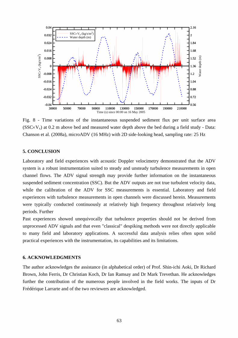
where qs and Vx are positive in the downstream direction. qs is a measure of the suspended sediment flux in the ADV sampling volume. Typical instantaneous suspended sediment flux per unit area results are presented in Figure 8 for a sampling volume located at 0.2 m above the bed. In such a small subtropical estuary, the sediment flux per unit area data showed typically an upstream, negative suspended sediment flux during the flood tide and a downstream, positive suspended sediment flux during the ebb tide. The data exhibited however considerable time-fluctuations that derived from a combination of velocity and suspended sediment concentration fluctuations. The integral time scale of the suspended sediment concentration data represents a characteristic time of turbid suspensions in the creek. Calculations were performed for two field studies in Australia. The SSC integral time scales seemed relatively independent of the tidal phase and yielded median SSC integral time scales TESSC of about 0.06 s. A comparison between the turbulent and SSC integral time scales showed some differences. The ratio of SSC to turbulence integral time scales was about 2 to 5 times lower during ebb tide periods, suggesting that the sediment suspension and suspended sediment fluxes were dominated by the turbulent processes during the flood tide, but not during the ebb tide.

63

Time (s) since 00:00 on 16 May 2005

SSC×V

x (kg

/s/m

2 )

Wat

er d

epth

(m)

30000 50000 70000 90000 110000 130000 150000 170000 190000 210000-0.04 0.56

-0.032 0.72

-0.024 0.88

-0.016 1.04

-0.008 1.2

0 1.36

0.008 1.52

0.016 1.68

0.024 1.84

0.032 2

0.04 2.16

30000 50000 70000 90000 110000 130000 150000 170000 190000 210000-0.04 0.56

-0.032 0.72

-0.024 0.88

-0.016 1.04

-0.008 1.2

0 1.36

0.008 1.52

0.016 1.68

0.024 1.84

0.032 2

0.04 2.16

SSC×Vx (kg/s/m2)Water depth (m)

Fig. 8 - Time variations of the instantaneous suspended sediment flux per unit surface area (SSC×Vx) at 0.2 m above bed and measured water depth above the bed during a field study - Data: Chanson et al. (2008a), microADV (16 MHz) with 2D side-looking head, sampling rate: 25 Hz

5. CONCLUSION

Laboratory and field experiences with acoustic Doppler velocimetry demonstrated that the ADV system is a robust instrumentation suited to steady and unsteady turbulence measurements in open channel flows. The ADV signal strength may provide further information on the instantaneous suspended sediment concentration (SSC). But the ADV outputs are not true turbulent velocity data, while the calibration of the ADV for SSC measurements is essential. Laboratory and field experiences with turbulence measurements in open channels were discussed herein. Measurements were typically conducted continuously at relatively high frequency throughout relatively long periods. Further Past experiences showed unequivocally that turbulence properties should not be derived from unprocessed ADV signals and that even "classical" despiking methods were not directly applicable to many field and laboratory applications. A successful data analysis relies often upon solid practical experiences with the instrumentation, its capabilities and its limitations.

6. ACKNOWLEDGMENTS

The author acknowledges the assistance (in alphabetical order) of Prof. Shin-ichi Aoki, Dr Richard Brown, John Ferris, Dr Christian Koch, Dr Ian Ramsay and Dr Mark Trevethan. He acknowledges further the contribution of the numerous people involved in the field works. The inputs of Dr Frédérique Larrarte and of the two reviewers are acknowledged.

64

8. REFERENCES

BLANCKAERT, K.,and LEMMIN, U. (2006). "Means of Noise reduction in Acoustic Turbulence Measurements." Jl of Hyd. Res., IAHR, Vol. 44, No. 1, pp. 3-17.

BRADSHAW, P. (1971). "An Introduction to Turbulence and its Measurement." Pergamon Press, Oxford, UK, The Commonwealth and International Library of Science and technology Engineering and Liberal Studies, Thermodynamics and Fluid Mechanics Division, 218 pages.

CHANSON, H. (2008). "Turbulence in Positive Surges and Tidal Bores. Effects of Bed Roughness and Adverse Bed Slopes." Hydraulic Model Report No. CH68/08, Div. of Civil Engineering, The University of Queensland, Brisbane, Australia, 119 pages & 5 movie files.

CHANSON, H., AOKI, S., and MARUYAMA, M. (2000). "Unsteady Two-Dimensional Orifice Flow: an Experimental Study." Coastal/Ocean Engineering Report, No. COE00-1, Dept. of Architecture and Civil Eng., Toyohashi University of Technology, Japan, 29 pages.

CHANSON, H., AOKI, S., and MARUYAMA, M. (2002). "Unsteady Two-Dimensional Orifice Flow: a Large-Size Experimental Investigation." Jl of Hyd. Res., IAHR, Vol. 40, No. 1, pp. 63-71.

CHANSON, H., BROWN, R., FERRIS, J., RAMSAY, I., and WARBURTON, K. (2005). "Preliminary Measurements of Turbulence and Environmental Parameters in a Sub-Tropical Estuary of Eastern Australia." Environmental Fluid Mechanics, Vol. 5, No. 6, pp. 553-575 (DOI: 10.1007/s10652-005-0928-y).

CHANSON, H., TREVETHAN, M., and KOCH, C. (2007). "Turbulence Measurements with Acoustic Doppler Velocimeters. Discussion." Journal of Hydraulic Engineering, ASCE, Vol. 133, No. 11, pp. 1283-1286 (DOI: 10.1061/(ASCE)0733-9429(2005)131:12(1062)).

CHANSON, H., TAKEUCHI, M., and TREVETHAN, M. (2008a). "Using Turbidity and Acoustic Backscatter Intensity as Surrogate Measures of Suspended Sediment Concentration in a Small Sub-Tropical Estuary." Journal of Environmental Management, Vol. 88, No. 4, Sept., pp. 1406-1416 (DOI: 10.1016/j.jenvman.2007.07.009).

CHANSON, H., TREVETHAN, M., and AOKI, S. (2008b). "Acoustic Doppler Velocimetry (ADV) in Small Estuary : Field Experience and Signal Post-Processing." Flow Measurement and Instrumentation, Vol. 19, No. 5, pp. 307-313 (DOI: 10.1016/j.flowmeasinst.2008.03.003).

FINELLI, C.M., HART, D.D., and FONSECA, D.M. (1999). "Evaluating the Spatial Resolution of an Acoustic Doppler Velocimeter and the Consequences for Measuring Near-Bed Flows." Limnology & Oceanography, Vol. 44, No. 7, pp. 1793-1801.

FUGATE, D.C., and FRIEDRICHS, C.T. (2002). "Determining Concentration and Fall Velocity of Estuarine Particle Populations using ADV, OBS and LISST." Continental Shelf Research, Vol. 22, pp. 1867-1886.

GARCIA, C.M., and GARCIA, M.H. (2006). "Characterization of Flow Turbulence in Large-Scale Bubble-Plume Experiments." Experiments in Fluids, Vol. 41, No. 1, pp. 91-101..

GORING, D.G., and NIKORA, V.I. (2002). "Despiking Acoustic Doppler Velocimeter Data." Journal of Hydraulic Engineering, ASCE, Vol. 128, No. 1, pp. 117-126. Discussion: Vol. 129,

65

No. 6, pp. 484-489. HINZE, J.O. (1975). "Turbulence." McGraw-Hill Publ., 2nd Edition, New York, USA. KARLSSON, R.I., and JOHANSSON, T.G. (1986). "LDV Measurements of Hihger Order

Moments of Velocity Fluctuations in a Turbulent Boundary Layer." Proc. 3rd Intl Symp. on Applications of Laser Anemometry to Fluid Mechanics, Libon, Portugal. (also Laser Anemometry in Fluid Mechanics III : Selected Papers from the Third International Symposium on Applications of Laser Anemometry to Fluid Mechanics, 1988, R.J. ADRIAN, D.F.G. DURAO, F. DURST, H. MISHINA and J.H. WHITELAW Ed., LADOAN-IST Publ., Chap. III, pp. 276-289.

KOCH, C., and CHANSON, H. (2005). "An Experimental Study of Tidal Bores and Positive Surges: Hydrodynamics and Turbulence of the Bore Front." Report No. CH56/05, Dept. of Civil Engineering, The University of Queensland, Brisbane, Australia, July, 170 pages.

KOCH, C., and CHANSON, H. (2008). "Turbulent Mixing beneath an Undular Bore Front." Journal of Coastal Research, Vol. 24, No. 4, pp. 999-1007 (DOI: 10.2112/06-0688.1).

KROGSTAD, P.A., ANDERSSON, H.I., BAKKEN, O.M., and ASHRAFIAN, A.A. (2005). "An Experimental and Numerical Study of Channel Flow with Rough Walls." Journal of Fluid Mechanics, Vol. 530, pp. 327-352.

LEMMIN, U., and LHERMITTE, R. (1999). "ADV Measurements of Turbulence: can we Improve their Interpretation ? Discussion" Journal of Hydraulic Engineering, ASCE, Vol. 125, No. 6, pp. 987-988.

LIU, M., ZHU, D., and RAJARATNAM, N. (2002). "Evaluation of ADV Measurements in Bubbly Two-Phase Flows." Proc. Conf. on Hydraulic Measurements and Experimental Methods, ASCE-EWRI & IAHR, Estes Park, USA, 10 pages (CD-ROM).

McLELLAND, S.J., and NICHOLAS, A.P. (2000). "A New Method for Evaluating Errors in High-Frequency ADV Measurements." Hydrological Processes, Vol. 14, pp. 351-366.

MARTIN, V., FISHER, T.S.R., MILLAR, R.G., and QUICK, M.C. (2002). "ADV Data Analysis for Turbulent Flows: Low Correlation Problem." Proc. Conf. on Hydraulic Measurements and Experimental Methods, ASCE-EWRI & IAHR, Estes Park, USA, 10 pages (CD-ROM).

NIKORA, V.I., and GORING, D.G. (1998). "ADV Measurements of Turbulence: can we Improve their Interpretation ?" Journal of Hydraulic Engineering, ASCE, Vol. 124, No. 6, pp. 630-634. Discusion: Vol. 125, No. 9, pp. 987-988.

NIKORA, V., and GORING, D. (2000). "Eddy Convection Velocity and Taylor's Hypothesis of 'Frozen' Turbulence in a Rough-Bed Open Channel Flow." Journal of Hydroscience and Hydraulic Engineering, Vol. 18, No. 2, pp. 75-91.

PIQUET, J. (1999). "Turbulent Flows. Models and Physics." Springer, Berlin, Germany, 761 pages. TREVETHAN, M. (2008). "A Fundamental Study of Turbulence and Turbulent Mixing in a Small

Subtropical Estuary." Ph.D. thesis, Dept of Civil Engineering, The University of Queensland, 342 pages.

TREVETHAN, M., CHANSON, H., and BROWN, R.J. (2007a). "Turbulence and Turbulent Flux Events in a Small Subtropical Estuary." Report No. CH65/07, Hydraulic Model Report series,

66

Div. of Civil Engineering, The University of Queensland, Brisbane, Australia, November, 67 pages.

TREVETHAN, M., CHANSON, H., and TAKEUCHI, M. (2007b). "Continuous High-Frequency Turbulence and Sediment Concentration Measurements in an Upper Estuary." Estuarine Coastal and Shelf Science, Vol. 73, No. 1-2, pp. 341-350 (DOI:10.1016/j.ecss.2007.01.014).

TREVETHAN, M., CHANSON, H., and BROWN, R. (2008). "Turbulence Characteristics of a Small Subtropical Estuary during and after some Moderate Rainfall." Estuarine Coastal and Shelf Science, Vol. 79, No. 4, pp. 661-670 (DOI: 10.1016/j.ecss.2008.06.006).

VOULGARIS, G., and TROWBRIDGE, J.H. (1998). "Evaluation of the Acoustic Doppler Velocimeter (ADV) for Turbulence Measurements." Journal Atmospheric and Oceanic Technologies, Vol. 15, pp. 272-289.

WAHL, T.L. (2003). "Despiking Acoustic Doppler Velocimeter Data. Discussion." Journal of Hydraulic Engineering, ASCE, Vol. 129, No. 6, pp. 484-487.