Embed Size (px)
Citation preview

Accounting Instructors’ ReportA Journal for Accounting Educators
Belverd E. Needles, Jr., Editor
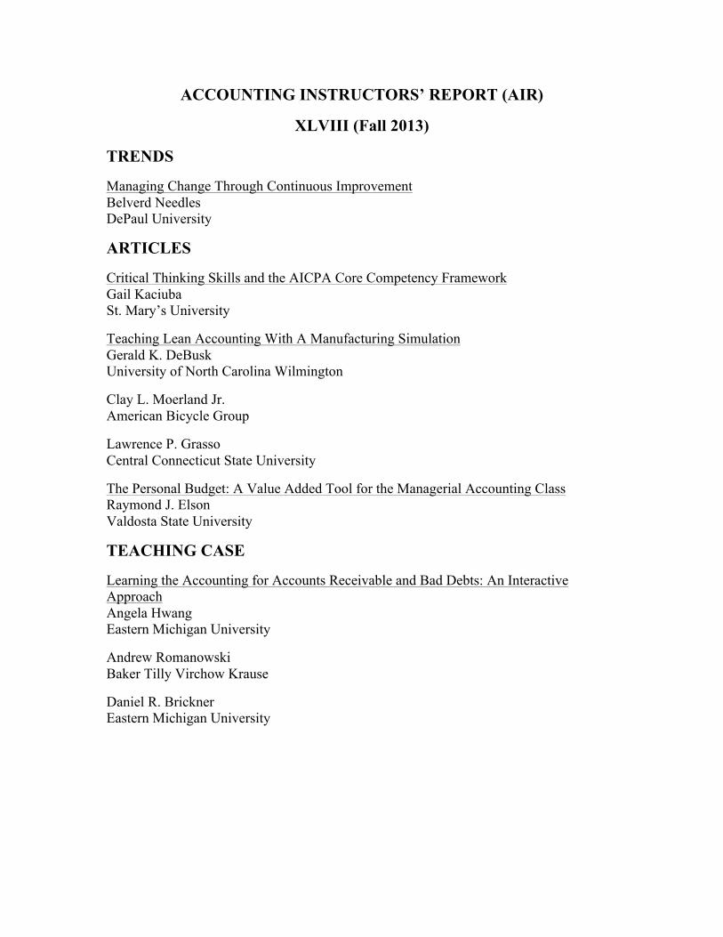
ACCOUNTING INSTRUCTORS’ REPORT (AIR)
XLVIII (Fall 2013)
TRENDS
Managing Change Through Continuous Improvement Belverd Needles DePaul University
ARTICLES
Critical Thinking Skills and the AICPA Core Competency Framework Gail Kaciuba St. Mary’s University
Teaching Lean Accounting With A Manufacturing Simulation Gerald K. DeBusk University of North Carolina Wilmington
Clay L. Moerland Jr. American Bicycle Group
Lawrence P. Grasso Central Connecticut State University
The Personal Budget: A Value Added Tool for the Managerial Accounting Class Raymond J. Elson Valdosta State University
TEACHING CASE
Learning the Accounting for Accounts Receivable and Bad Debts: An Interactive Approach Angela Hwang Eastern Michigan University
Andrew Romanowski Baker Tilly Virchow Krause
Daniel R. Brickner Eastern Michigan University

1
CRITICAL THINKING SKILLS AND THE AICPA CORE COMPETENCY FRAMEWORK
Gail Kaciuba, PhD
Emil Jurica Professor of Accounting Bill Greehey School of Business
St Mary’s University 1 Camino Santa Maria
San Antonio, TX 78228 [email protected]

1
CRITICAL THINKING SKILLS AND THE AICPA CORE COMPETENCY FRAMEWORK
INTRODUCTION
In most schools, accounting principles courses are for accounting majors as well as all
other business majors. As educators, we want to make sure the accounting majors graduate with the skills they will need in the profession. However, we also want to provide non-accounting majors with the basic accounting knowledge they will need in their future careers. Additionally, we should aspire to improve the critical thinking skills of all students, regardless of major. The AICPA Core Competency Framework (CCF) provides a comprehensive list of the competencies the profession demands of entry-level accountants (AICPA, 2005). The Steps for Better Thinking (SBT) Model (Lynch & Wolcott, 2001) provides a way to assess the critical thinking skills of students in college. These two constructs actually relate to one another, which means that we can provide skill improvement opportunities for all students in accounting principles courses, regardless of their majors.
This paper begins with a review of the CCF and then provides a review of the SBT
Model. Then the reasons these two constructs are related are covered. The paper then includes suggestions as to how educators can use these two frameworks in accounting principles courses, with the competency addressed shown in parentheses.
THE AICPA CORE COMPETENCY FRAMEWORK
An interesting article that is forthcoming in Issues in Accounting Education covers the
history of the calls for reform in accounting education (Black, 2013). Apparently, the first issue of Journal of Accountancy in 1905 contained an article about improvements in accounting education the author felt were necessary in order for accountancy to be considered a profession. More recently though, most accounting education articles start with the mention of the Bedford Report (AAA, 1986) and the Accounting Education Change Commission (AECC), a group of accounting educators and members of the profession (AECC, 1990). In general, these actions arose from the profession noting that entry-level accountants need more skills than just memorized knowledge of accounting principles and procedures.
The AICPA CCF came from the CPA Vision Project, in which over 3,300 accounting
professionals participated in forums to discuss the future of the profession1. The CCF lists several competencies needed by students entering the profession, and groups these competencies into three categories:
• Broad Business Perspectives Competencies—perspectives and skills relating to understanding of internal and external business contexts
• Functional Competencies—technical competencies most closely aligned with the value contributed by accounting professionals
• Personal Competencies—individual attributes and values 1 http://www.aicpa.org/Research/CPAHorizons2025/CPAvisionProject/Pages/CPAVisionProject.aspx, accessed August 10, 2013.

2
There are several competencies in each category. The ‘Leverage Technology’ competency is in all three categories. Most of the competencies listed in each category are valuable skills for all business majors. For example, the Broad Business Perspective category includes strategic/critical thinking, the ability understand the risks and opportunities in an industry or sector, the ability to understand the global marketplace, an appreciation of resource constraints, an understanding of the legal and regulatory environment, and the ability to meet the changing needs of clients and employers.
Clearly, all business professionals need these skills. The Personal Competencies
category similarly contains skills all business students will need, such as the ability to work professionally in teams, communication skills, decision-making abilities, and project management skills. Only the Functional Competencies category contains some skills that might apply more to accounting students than other business students (but of course, these skills would still benefit all business students).
THE STEPS FOR BETTER THINKING MODEL
The Reflective Judgment (RJ) Model is a well-known, full-life stage, model of cognitive
development (King & Kitchener, 1994). One drawback of the RJ Model was the methodology for obtaining assessment data on subjects. Assessors must be certified RJ interviewers or essay readers. Susan Wolcott and Cindy Lynch, with the support and guidance of King & Kitchener, developed the SBT Model for use on college-age subjects (Lynch & Wolcott, 2001; Wolcott & Lynch, 2002; Wolcott, 2005). The assessment rubrics for the SBT Model are easier to use and anyone can learn to use them. These rubrics can also be used on traditional course assignments with only minor changes to the assignments.
The SBT Model has five levels of performance, called steps, from step 0 through step 4. Students develop these skills sequentially, which means that a student at step 1 is unable to display step 3 skills. However, as students progress through these developmental steps, they may display some skills at, for example, step 1 and step 2. In this case, such a student would be categorized as being at the step 1.5 level of cognitive development. Figure 1 shows a graphical representation of the SBT Model.
Both the RJ and SBT Models are based on students’ beliefs as to where knowledge
comes from. A student at step 0 (shown as ‘foundation’ on Figure 1) believes that knowledge comes from experts (i.e. professors). It is the professor’s job to share his knowledge and it is the student’s job to memorize this wisdom. Eventually a student at step 0 recognizes that even experts disagree. This student now promotes himself to ‘expert’. He will read a scenario, ignore any information that doesn’t support his determination of the ‘truth’, and then cite the remaining evidence as proof that he is right.
Gradually, a student at step 1 realizes that he is not the expert, and all points of view have
some validity (in other words, truth is relative). This step 2 student can analyze the pros and cons of alternatives but has difficulty making a decision amongst the alternatives. When this student can finally weigh the pros and cons of the alternatives and make and defend a decision,
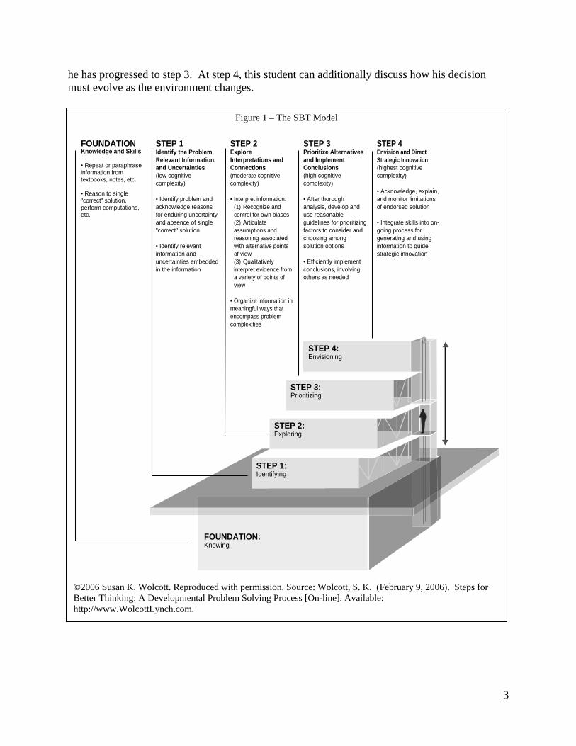
3
he has progressed to step 3. At step 4, this student can additionally discuss how his decision must evolve as the environment changes.
Figure 1 – The SBT Model
©2006 Susan K. Wolcott. Reproduced with permission. Source: Wolcott, S. K. (February 9, 2006). Steps for Better Thinking: A Developmental Problem Solving Process [On-line]. Available: http://www.WolcottLynch.com.
FOUNDATIONKnowledge and Skills
• Repeat or paraphraseinformation fromtextbooks, notes, etc.
• Reason to single"correct" solution,perform computations,etc.
STEP 1Identify the Problem,Relevant Information,and Uncertainties(low cognitivecomplexity)
• Identify problem andacknowledge reasonsfor enduring uncertaintyand absence of single"correct" solution
• Identify relevantinformation anduncertainties embeddedin the information
STEP 2ExploreInterpretations andConnections(moderate cognitivecomplexity)
• Interpret information:(1) Recognize andcontrol for own biases(2) Articulateassumptions andreasoning associatedwith alternative pointsof view(3) Qualitativelyinterpret evidence froma variety of points ofview
• Organize information inmeaningful ways thatencompass problemcomplexities
STEP 3Prioritize Alternativesand ImplementConclusions(high cognitivecomplexity)
• After thoroughanalysis, develop anduse reasonableguidelines for prioritizingfactors to consider andchoosing amongsolution options
• Efficiently implementconclusions, involvingothers as needed
STEP 4Envision and DirectStrategic Innovation(highest cognitivecomplexity)
• Acknowledge, explain,and monitor limitationsof endorsed solution
• Integrate skills into on-going process forgenerating and usinginformation to guidestrategic innovation
STEP 4:Envisioning
STEP 3:Prioritizing
STEP 2:Exploring
STEP 1:Identifying
FOUNDATION:Knowing

4
THE EDUCATIONAL COMPETENCY ASSESSMENT WEBSITE
The AICPA created the Educational Competency Assessment (ECA) website to help accounting educators include classroom activities that will emphasize the competencies in the CCF2. The most useful aspect of this website is that it contains examples of abilities students should exhibit in order to show mastery of that competency. More importantly, each example has a label indicating the level of performance (levels 1 through 4). Susan Wolcott created the ECA website content, and levels 1 through 4 directly correspond to steps 1 through 4 of the SBT Model. The SBT Model is a model of cognitive development, and applies to competencies other than critical thinking.
It is important for educators to remember that students develop thinking skills
sequentially. We might believe it would be great to have an assignment that asks students to analyze the pros and cons of alternatives (a step 2 skill). However, if most of the students in the class are at step 0, this will be a frustrating exercise for both professors and students. When most of the students are at step 0, we should ask students to respond to questions aimed at step 0 and step 1 (to give them practice developing skills at the next level).
We know from assessment data gathered from the RJ and SBT Models over the years that students leave a four-year college career at an average of step 0.99 (King & Kitchener, 1994, Table 6.6). However, this is an average of all students; there are no data specific to business majors. After years of using the SBT model, I believe that business majors graduate at a slightly higher level, but this is only anecdotal. Regardless, the implication for instructors of accounting principles courses is that they should provide assignments and activities targeted at only step 0 and step 1. Most students in accounting principles are likely at step 0. However, if we provide classroom activities aimed at the students’ developmental level, and at one higher level, we may be able to speed up this cognitive developmental process (Fischer & Bidell, 1998; Wolcott & Lynch, 2002).
Table 1 shows examples of level 1 skills for all the Broad Business Perspective (BBP)
competencies in the CCF, except for ‘Leverage Technology’, which is covered at the end of this paper. Instructors can give students practice on most of these competencies by assigning homework problems found in the textbooks, often with very few changes. For example, instructors can cover the BBP competency ‘Industry/Sector Perspective’ in the cost-volume-profit (CVP) chapter. The instructor can assign a CVP problem in one industry that is capital intensive, and another problem in an industry that is labor intensive. Then ask students in a class discussion to compare and contrast these two industries. Which is more risky? Students should be able to identify the financial risks of the capital-intensive company, and instructors should guide them to consider other risks. Is one industry subject to more regulation that is frequently changed? Is there more competition in one industry? What other risks might a company face in each industry? (BBP-Industry/Sector Perspective).
Most accounting principles texts cover global business issues in several chapters, often in
the first chapter that introduces managerial accounting. The instructor can choose a homework 2 http://www.aicpa-eca.org/default.asp, accessed August 15, 2013. You must register to use this site, but registration is free.

5
problem with an international scenario. Assigning students to teams and giving them five to ten minutes to list several global issues relevant to this scenario can lead to a fun class discussion. When the teams present their lists to the class, students are more engaged as they wonder if another team thought of something their team did not (BBP-International/Global Perspective).
When covering contingent liabilities, start a class discussion about how an organization
should respond when being sued, using some scenario from the news or the text. During this discussion, concentrate on the uncertainties the organization faces. For example, the entity might consider settling out of court, but it can’t be sure what amount to offer. It also can’t be sure of the reputational effects of settling, or the outcome in court if it does not settle (BBP-Legal/Regulatory Perspective). One of the best ways to build level 1 skills is to make students consider uncertainties (Fisher & Bidell, 1998). Another idea is to use a recent news story about a business’ response to the upcoming Affordable Care Act. There are many uncertainties about this, as many of the regulations are not yet written and various aspects of the statute are being postponed at the last minute (BBP-Legal/Regulatory Perspective).
If activity-based costing is covered in your principles courses, students can do a customer
profitability analysis in class, followed by a discussion as to the reasons the customer may or may not decide to continue doing business with the company. The discussion should include consideration as to whether the company should maintain that customer. While covering the job order costing chapter, instructors can include examples about special demands of customers and how the costs of these demands should be captured (BBP-Marketing/Client Focus).
Table 1 – Examples of Level 1 Skills in the Broad Business Perspective Category of the CCF Industry/Sector Perspective • Identifies the economic, broad business, and financial risks of the industry/sector International/Global Perspective • Identifies global issues relevant to a business decision Legal/Regulatory Perspective • Identifies uncertainties about how an organization should respond to a legal/regulatory issue • Identifies reasons why the legal/regulatory environment might change Marketing/Client Focus • Identifies factors that motivate internal and external customers to enter into relationships or continue
doing business with an organization • Articulates uncertainties about relationships with internal and external customers (T) Resource Management • Explains why there are uncertainties about the availability and alternatives uses of resources (B) Strategic/Critical Thinking • Identifies and gathers data from a wide variety of sources for decision-making (T) Refer to ‘teamwork’ discussion in the paper (B) Refer to ‘budgeting’ discussion in the paper Source: http://www.aicpa-eca.org/default.asp. Not all examples of level 1 skills are shown in this table.
Table 2 shows examples of level 1 competencies for the Functional (F) competencies category (except for ‘Leverage Technology’). Choose a homework problem in almost any area and ask students to list the uncertainties. For example, have students work on an accept/reject special orders problems in class and cover both situations of existing idle capacity and no idle

6
capacity. Then facilitate a class discussion about how this situation could be analyzed (incremental analysis versus a full recast of the income statement budget). What uncertainties does the company face (e.g. what amount would the potential customer be willing to pay, what alternatives does the customer have, is the measure of capacity static or dynamic, and are the estimates of future costs accurate)? (F-Decision Modeling).
Table 2 – Examples of Level 1 Skills in the Functional Competencies Category of the CCF
Decision Modeling • Identifies problems, potential solution approaches, and related uncertainties (B) Measurement • Describes uncertainties about data and how items should be measured Reporting • Lists types of information relevant to a given report (B) Research • Explains why there are uncertainties about the interpretation of information, including existing rules • Employs relevant research skills for locating data Risk Analysis • Explains why controls cannot completely eliminate risk of negative outcomes (B) Refer to ‘budgeting’ discussion in the paper Source: http://www.aicpa-eca.org/default.asp. Not all examples of level 1 skills are shown in this table. After you cover the statement of cash flows, have students make a list of the information that is needed (and where they need to go to get this information) to create the statement. Most of the information they list will be items from the income statement and the changes in the comparative balance sheets, but not all of it (F-Reporting).
Table 3 – Examples of Level 1 Skills in the Personal Competencies Category of the CCF
Communication • Expresses information and concepts with conciseness and clarity when writing and speaking (T) Interaction • Commits to achievement of common goals when working on a team (T) Leadership • Identifies the various leadership styles (B) Problem Solving/Decision Making • Identifies uncertainties about the interpretation or significance of information and evidence Professional Demeanor • Identifies ethical dilemmas (T) Project Management • Identifies project goals (T) Refer to ‘teamwork’ discussion in the paper (B) Refer to ‘budgeting’ discussion in the paper Source: http://www.aicpa-eca.org/default.asp. Not all examples of level 1 skills are shown in this table.

7
Accounting principles texts usually have a chapter about internal controls or accounting information systems. At any stage of this chapter, for any control, facilitate a discussion about why that control may not prevent or detect the misstatement as designed (F-Risk Analysis). Table 3 shows examples of level 1 competencies in the Personal (P) competencies category (except ‘Leverage Technology’). Choose any homework problem that asks students to write a memo. Be sure to score these memos for grammar, style and punctuation, so that students get the feedback they need to improve their writing skills (P-Communication). Similarly, many homework problems in texts ask students to identify the ethical dilemma in a situation. Make sure that you ask them to explain why it is a dilemma (P-Professional Demeanor). Tables 1 through 3 show several competencies marked with a (B). There is an exercise that I like to give before we cover the budgeting chapter, and it gives students practice with several competencies in all three CCF categories. Students can do this exercise individually, but I prefer a group assignment. Have students create a budget for a fictional student, and provide some facts of her situation. Maybe she lives on campus or off campus. Maybe she gets student aid or she doesn’t. Ask them to prepare a 12-month budget for this student. They will need to research the costs of apartments in the area or on-campus housing alternatives, as well as parking options, food options, and the like (BBP-Strategic/Critical Thinking and F-Research).
In the assignment, ask them to consider how much uncertainty there is surrounding their estimates (the estimate of tuition costs likely came from the university website, so there is very little uncertainty in that estimate, but they needed to make a number of assumptions about living arrangements, so there is much more uncertainty surrounding the housing costs estimate). (P-Problem Solving/Decision Making). As another example, ask them how they determined whether to include car insurance when they weren’t told if the student even owned a car. Ask them to make complete lists of the assumptions they made and why they made those assumptions. Also ask them how they determined the monthly amounts – did they put the full 6-month car insurance premium in only the months it needs to be paid or did they average it over 6 months? Why did they do it that way? (F-Measurement and P-Problem Solving/Decision Making). Students may express some frustration during this class discussion, and complain that the assignment’s instructions were not specific enough, but they will learn a lot. All competencies marked with (T) in Tables 1 through 3 can be covered with any group assignment, and the budgeting assignment described above is a perfect example. In the group assignment, ask students to provide written responses to several questions. What resources did you have in your team (for example, maybe one or more team members was good with Excel, or maybe some had first-hand knowledge about off-campus housing costs). (BBP-Resource Management). Also ask each individual team member to describe the team’s goals and his contributions to them (P-Interaction and P-Project Management). Before you assign this group project, describe to students various types of leadership styles. Afterwards, ask them to identify which team member was the group’s leader and which leadership style that person used (P-Leadership).

8
As mentioned earlier, the ‘Leverage Technology’ competency is in all three categories of the CCF (although it was omitted from Tables 1 through 3). As you might imagine, students are likely more advanced in this competency than many of us! The use of email and Blackboard or Web-CT discussion boards, or a spreadsheet assignment, target level 1 of this competency.
CONCLUSION
The AICPA CCF includes competencies necessary for all business students, not just accounting majors. By designing classroom activities targeted at the appropriate level of development, we can improve competency development in all our students. This paper concentrated on the accounting principles courses, but the ECA website shows examples for all four performance levels for all of the CCF competencies, and instructors can choose activities that target level 2 for their intermediate accounting courses. In senior year accounting courses, instructors can work on developing competencies at higher levels. See the Kaciuba (2012) paper for an example group auditing project that targets many higher performance levels of these competencies.
It would be helpful to know the SBT Model’s performance level of your students as you
plan assignments and activities. The Wolcott/Lynch website (www.WolcottLynch.com) contains scoring rubrics and guidance to help you accomplish this.

9
REFERENCES
Accounting Education Change Commission (AECC), (1990). Position statement number one: Objectives of education for accountants. Issues in Accounting Education, Fall. 307-312.
American Accounting Association Committee on the Future Structure, Content, and Scope of
Accounting Education (The Bedford Committee) (1986). Future accounting education: Preparing for the expanding profession. Issues in Accounting Education, Vol. 1, 168-195.
American Institute of Certified Public Accountants (AICPA), (2005). AICPA core competency
framework for entry into the accounting profession. http://www.aicpa.org/interestareas/accountingeducation/resources/pages/corecompetency.aspx. Accessed August 4, 2013.
Black, W. (2013). The Activities of the Pathway’s Commission and the Historical Context for
Changes in Accounting Education. Forthcoming in Issues in Accounting Education. Fischer, K. W., & Bidell, T. R. (1998). Dynamic development of psychological structures in
action and thought. In R. M. Lerner (Ed.), & W. Damon (Series Ed.), Handbook of child psychology (Vol. 1, pp. 467–531). Theoretical models of human development (5th ed.). New York: Wiley.
Kaciuba, G. (2012). An instructional assignment for student engagement in auditing class:
Student movies and the AICPA Core Competency Framework. Journal of Accounting Education, Vol. 30, Issue 2, pp. 248-266.
King, P. M., & L. S. Kitchener, K. S. (1994). Developing Reflective Judgment: Understanding
and Promoting Intellectual Growth and Critical Thinking in Adolescents and Adults. San Francisco: Jossey-Bass.
Lynch, C. & Wolcott, S. (2001). Helping your students develop critical thinking skills, IDEA
Paper No. 37, http://www.theideacenter.org/sites/default/files/IDEA_Paper_37.pdf. Accessed July 2, 2012.
Wolcott, S. K., & Lynch, C. L. (2002). Developing critical thinking skills: The key to
professional competencies. A faculty handbook and tool kit. Sarasota, FL: American Accounting Association.
Wolcott, S. K. (2005). Assessment of critical thinking, in: Calderon, T. G., Martell, K. D. (Eds.),
Assessment of student learning in business schools: Best practices each step of the way, Vol. 1, Association for Institutional Research and AACSB International, Florida.

1
TEACHING LEAN ACCOUNTING WITH A MANUFACTURING SIMULATION
Gerald K. DeBusk, Ph.D., CPA, CMA, CGMA Associate Professor of Accounting
University of North Carolina Wilmington Cameron School of Business
601 S. College Road Wilmington, NC 28403-5901
Clay L. Moerland, Jr. Cost Accountant
American Bicycle Group 9308 Ooltewah Industrial Blvd.
Ooltewah, TN 37363 [email protected]
423-591-8778
Lawrence P. Grasso, D.B.A. Professor and Accounting, Department Chair
Central Connecticut State University School of Business
1615 Stanley Street, P.O. Box 4010 New Britain, CT 06050-4010
[email protected] 860-832-3226
Acknowledgements: The authors wish to thank the following University of Tennessee at Chattanooga executive MBA students for their help with testing the simulation and allowing their photographs to be used: Kendell Lewis, Joe Painter, Mike Spachtholz, Scott Lakey, and Chris Reneau. We would also like to acknowledge the late Dr. Stan Davis for his invaluable assistance, encouragement, and support.

2
INTRODUCTION
Lean Accounting evolved in order to promote goals consistent with the Lean philosophy. It has been accepted by companies for its ability to create accurate, useful, real-time financial data, useable by both managers and line employees. Correspondingly, Lean Accounting is more frequently included as a topic in university management accounting courses. We use a modified version of Peter J. Billington’s airplane manufacturing simulation, “A Classroom Exercise to Illustrate Lean Manufacturing Pull Concepts”, to introduce students to Lean Accounting (Billington, 2004). This teaching note is intended to help the reader run a Lean simulation, develop Lean Accounting Profit & Loss statements, and compare Lean Accounting profits to absorption costing profit. It also analyzes the behaviors encouraged by each method.
Prior studies have shown that 40% of organizations are pursuing a Lean strategy or philosophy (DeBusk & DeBusk, Characteristics of Successful Lean Six Sigma Organizations, 2010) (DeBusk & DeBusk, Combining Hoshin Planning with the Balanced Scorecard to Achieve Breakthrough Results in Lean Six Sigma Organizations, 2011). These studies have also shown that many organizations are struggling with adapting their management accounting systems to the Lean philosophy (DeBusk & DeBusk, Has Your Accounting Department Evolved? Accounting and the Use of Lean Six Sigma, 2011). Traditional management accounting systems are often standard costing systems, developed when mass production was common. Standard costing systems encourage behavior in conflict with Lean by rewarding overproduction. Overproduction gets rewarded through the deferral of fixed overhead costs and the extra standard credit earned for efficiency variance calculations. Standard cost systems also penalize management when inventory levels are drawn down by recognizing as current expenses the costs previously deferred in inventory accounts. A key to successfully implementing Lean manufacturing is to use a Lean Accounting approach. In this way, the performance measurement systems are consistent with the Lean management strategy or philosophy.
The simulation has been performed in MBA managerial accounting courses but can be used in a variety of settings. After participating in or witnessing the simulation, the student should:
• Understand how Theory of Constraints affects flow through a manufacturing process. • Understand how Lean Manufacturing leads to improved flow and Work-in-Process
reductions. • Understand how absorption costing and traditional performance measures reward
overproduction. • Understand how Lean Accounting promotes goals consistent with the Lean philosophy
like conservation of resources.
Students make paper airplanes using two methodologies, mass production and Lean Manufacturing. Theory of Constraints explains why both methods produce 20 airplanes in about the same amount of time. Little’s Law explains how a single airplane is produced much quicker using Lean and a kanban system. Profit and Loss statements are prepared for both production runs. Under Generally Accepted Accounting Principles (GAAP), the mass production run appears more profitable. The student, after the simulation, will understand that this is due to the allocation of fixed costs to the extra production. These costs are deferred in inventory and not

3
recognized on the Profit and Loss statement. The additional resources expended (e.g. material costs) are also deferred. Students learn several of the costs deferred by GAAP are recognized when incurred with Lean Accounting. This trait of Lean Accounting helps focus the organization on not expending resources until necessary and is consistent with Lean’s philosophy of building to customer demand. Students also see that Lean Accounting is much simpler than traditional methods and provides information in a plain-English format that is more useful for decision making.
PRODUCTION SIMULATION
Similar to Peter J. Billington’s article “A Classroom Exercise to Illustrate Lean Manufacturing Pull Concepts”, we have four students in four work centers manufacture paper airplanes (Billington, 2004). They are assembly workers for GCL Aerospace Company. Each production run produces twenty finished airplanes, nineteen regular and one special order (denoted by using a sheet of differently colored paper). We have raw material supplied to the line in the form of numbered sheets of paper.
Production Run #1
In the first production run (Production Run #1 – Mass Production), students should be encouraged to produce as many as possible at each work center. The process at each station should be similar to Billington’s article with the third work center designed to be the constraint or bottleneck. In Billington’s article, work center 1 will fold the paper in half, work center 2 will fold down the front left corner and front right corner as the first fold for the wings, work center 3 will make the second folds for the wings and mark the plane with an identification number or symbol (indicated by a star in Figure 11), work center 4 will make the third fold of the wings. (Billington, 2004) See Figure 1. We suggest letting the participating students practice on a couple of scrap sheets of paper. The practice should lessen the effects of any learning curve on the outcomes. Students not participating should track the total time of each production run as well as the total time for a special order (described below). See Table 1.
1 One of the authors often uses the course number here and has the number recorded on both sides of the plane. This lengthens the task being done at work center 3 and helps insure it will be the bottleneck.

4
FIGURE 1: WORK INSTRUCTIONS
Work Station 1: Fold paper lengthwise
Work Station 2: Front corner folds
Work Station 3: First side folds, stars on sides
Work Station 4: Final side folds

5
TABLE 1: TIMESHEET
PRODUCTION RUN: Production
Run #1
Production Run #2
Start Time:
End Time (20th plane finished):
Elapsed Time:
Avg. Time per Plane (Elapsed / 20)
SPECIAL ORDER: Start Time:
End Time:
Elapsed Time:
WORK IN PROCESS INVENTORY
Planes through Work Center 1:
Planes through Work Center 2:
Planes through Work Center 3:
Total:
We suggest having 33 numbered sheets of paper (raw material) on hand for Production Run #1. The 20th sheet should be a different color from the rest and will be designated a “special”. Before starting each production run, the instructor should “prime” the production line with the numbered paper. Priming the line is where production is done without being timed to fill the line with work in process (WIP). Production for any period rarely begins with the line completely dry of WIP. We recommend starting each production run with one unit of WIP after each of the first three work centers. Work center 1 will pull the 4th sheet of paper/raw material from inventory when timed production begins. Each production run will be to produce 20 finished airplanes in order (First-In-First-Out). One of the airplanes will be a special, designated with a sheet of differently colored paper, and also separately timed. We recommend placing the special as the 20th unit so that students can readily see when production should cease. The colored sheet of paper also makes it easy for students to track and time the plane’s production.
Production Run #1 will simulate mass production with workers focusing on producing as much as possible through their work center – a silo approach. Production Run #1 will result in inventory building in front of the bottleneck work center (work center 3). See Figure 2. The First-In-First-Out (FIFO) flow assumption will cause some problems for the students because they must stack finished production in such a way as to allow the next work center to manufacture in the correct order. With only 33 total numbered sheets of paper, work center 1

6
should easily process all available raw materials and be idle the rest of the run.2 Therefore, Run #1 should end with 13 pieces of Work-In-Process (WIP) inventory.
FIGURE 2: INVENTORY (WIP) BUILDING IN FRONT OF CONSTRAINT
Discussion of Production Run #1
After the production run has been completed, students (participants and observers) should be asked about the process. Students should realize after this exercise that the line as a whole can only produce as fast as the constraint/bottleneck (Theory of Constraints). They should also realize the futility of producing faster than the constraint in upstream work centers. The faster work centers 1 and 2 produce, the more WIP is created because no additional throughput can be achieved through the constraint, work center 3. Discuss with students the “real” costs associated with overproduction after the first run. These costs include storage costs, costs of capital, risk of obsolescence, etc. For simplicity, we do not include these costs as part of the exercise; however, we feel they should be discussed. The instructor may also discuss how the excess WIP affected the process. Did the rising queue in front of work center 3 make it more difficult to work? Was the worker discouraged? Did it cause the worker to rush and reduce the quality of the output?
Production Run #2
Production Run #2 will use a kanban system (kanban is a Japanese term that loosely translates as production signal) to synchronize the production of all work centers and mimic a pull system, common in Lean production. This is illustrated by having a designated open space in front of work centers 2, 3, and 4. Work center 1 should produce one piece of inventory when
2 We hold the total raw materials to 33 sheets of paper to simplify the comparison between the two runs and to not needlessly waste paper. If you want to highlight the potential for inventory buildup to be even worse, then have another student measure the down time in the first cell due to lack of material.

7
the blank space is empty, the same for work centers 2 and 3. Work center 4 (downstream from the constraint/bottleneck) will process any units available. See Figure 3. We will assume that the customer is waiting on the airplane. This synchronization of the work centers limits the number of planes that can be in WIP to three.
FIGURE 3: PRODUCTION RUN USING KANBAN SYSTEM
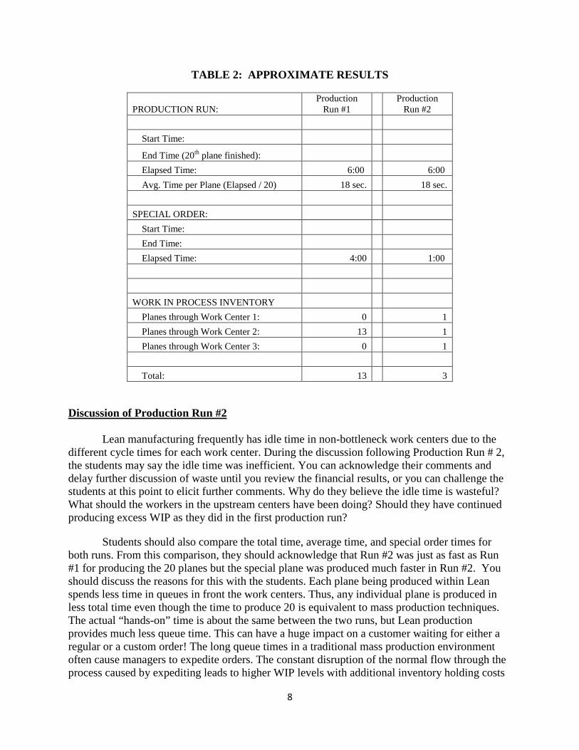
Table 2 contains approximate times and WIP inventory levels for the two production runs.3 Typically students manufacture the 20 airplanes in about the same length of time for both runs as predicted by Theory of Constraints. Production Run #1 utilizes the extra time of the non-constrained work centers upstream of the constraint to produce additional WIP. Production Run #2 does NOT utilize the extra time for production. This should not slow down the production of the 20 airplanes as the bottleneck work center (work center 3) is continuously supplied with material due to the faster processing times of work centers 1 and 2. The special order time is much faster with the Lean manufacturing run because the special has less wait time at each work center.
3 The results in Table 2 reflect our experience running this version of the simulation in MBA classes and a seminar (4 trials) over a 12 month period. The times may be slightly elevated because a course number or similar graphic was required to be written on both sides of the plane in work station 3. As stated in an earlier footnote, this tactic insures that work station 3 is the bottleneck but will slow production slightly.
8
TABLE 2: APPROXIMATE RESULTS
PRODUCTION RUN: Production
Run #1
Production Run #2
Start Time:
End Time (20th plane finished):
Elapsed Time: 6:00
6:00
Avg. Time per Plane (Elapsed / 20) 18 sec.
18 sec.
SPECIAL ORDER: Start Time:
End Time:
Elapsed Time: 4:00
1:00
WORK IN PROCESS INVENTORY
Planes through Work Center 1: 0
1 Planes through Work Center 2: 13
1
Planes through Work Center 3: 0
1
Total: 13
3
Discussion of Production Run #2
Lean manufacturing frequently has idle time in non-bottleneck work centers due to the different cycle times for each work center. During the discussion following Production Run # 2, the students may say the idle time was inefficient. You can acknowledge their comments and delay further discussion of waste until you review the financial results, or you can challenge the students at this point to elicit further comments. Why do they believe the idle time is wasteful? What should the workers in the upstream centers have been doing? Should they have continued producing excess WIP as they did in the first production run?
Students should also compare the total time, average time, and special order times for both runs. From this comparison, they should acknowledge that Run #2 was just as fast as Run #1 for producing the 20 planes but the special plane was produced much faster in Run #2. You should discuss the reasons for this with the students. Each plane being produced within Lean spends less time in queues in front the work centers. Thus, any individual plane is produced in less total time even though the time to produce 20 is equivalent to mass production techniques. The actual “hands-on” time is about the same between the two runs, but Lean production provides much less queue time. This can have a huge impact on a customer waiting for either a regular or a custom order! The long queue times in a traditional mass production environment often cause managers to expedite orders. The constant disruption of the normal flow through the process caused by expediting leads to higher WIP levels with additional inventory holding costs

9
and additional setup costs, all in addition to the costs of tracking and expediting. Lean’s faster flow allows organizations to cut back on expediting.
See Figure 4 for a photograph depicting what the constraint (work center 3) looks like during Lean production.
FIGURE 4: LOWER INVENTORY (WIP) LEVELS IN PRODUCTION RUN #2 – PICTURE OF THE CONSTRAINT
With Production Run #2, we implemented a kanban system but made no further improvements. Additional runs can be made after allowing students to rebalance the line (e.g. shift work from the constraint to other work centers). These additional improvements should shorten the production time for all 20 airplanes.

10
FINANCIALS
TABLE 3: FINANCIAL INFORMATION FOR GCL AEROSPACE COMPANY
Selling price $3,000 / unit Material costs $1,000 / unit Conversion Costs (Beg. WIP) $1,500 / unit
Fixed Costs Conversion
Costs S&A Costs
Total Fixed Costs
Payroll & Fringes $7,500 $7,500 Supplies $500 $500 Equipment depreciation $8,000 $8,000 Facility costs $10,000 $10,000 Sustaining $4,000 $5,000 $9,000 Total $30,000 $5,000 $35,000
The costs shown in Table 3 can be used to calculate P&Ls (Profit and Loss Statements) and to value inventory based on the actual results from your specific simulation. However, the financial results that follow should be expected. By controlling the amount of raw material available, the instructor can more or less script the financial statements ahead of time. We use data from Tables 2 and 3 to calculate cost flows, P&Ls, and inventory valuations. We assumed in the short run, all costs outside of direct materials are fixed. The fixed conversion cost assumption is consistent with Eliyahu Goldratt’s Theory of Constraints (TOC) and Throughput Accounting; as well as, Lean theory. We also assume all airplanes produced are for customer orders and therefore sold.

11
Absorption Costing
TABLE 4: GCL AEROSPACE CO. ABSORPTION COSTING WIP T-ACCOUNTS
The absorption costing WIP T-account is provided in Table 4 along with supporting computations for both production runs and is based on the cost data in Table 3 and the production data from Table 2. We assume that beginning and ending WIP inventory is 100% complete for material and 50% complete as to conversion costs. The inventory costing can be solved easily through the use of process costing techniques. We chose to use the First-In-First-Out (FIFO) method. See the appendices for the detail worksheets. For simplicity, standard costing is not used. However, we discuss standard costing and variances. Students should be reminded that process costing and standard costing will produce similar results at the end of the year, when variances are allocated to inventory and cost of goods sold.
Production Run #1
Average Conversion Costs per Unit Computations$30,000 Conversion Costs per Period a M = $3,000 = $1,000 * 3 units
1.5 Eq. Units to Finish BI (3 @ 50%) C = $2,250 = $1,500 * 3 units * 50%17 Additional Eq. Units Started & Completed T = $5,250 = $3,000 + $2,2506.5 Additional Eq. Units Started but Not Finished (EI) b $1,000 * 30 units started into production25 Total Equivalent Units c Given/Fixed
$1,200 Average Conversion Costs per Unit d $5,250 + ($1,200 * 3 units * 50%)
e M = $17,000 = $1,000 * 17 unitsC = $20,400 = $1,200 * 17 units
BI $5,250 a T = $37,400 = $17,000 + $20,400M $30,000 b f EI = BI + M + C - CoGS orC $30,000 c M = $13,000 = $1,000 * 13 units
CoGS-BI $7,050 d \ C = $7,800 = $1,200 * 13 units * 50%CoGS-S&C $37,400 e / T = $20,800 = $13,000 + $7,800
EI $20,800 f
$44,450
WIP - Run # 1
Production Run #2
Average Conversion Costs per Unit Computations$30,000 Conversion Costs per Period a M = $3,000 = $1,000 * 3 units
1.5 Eq. Units to Finish BI (3 @ 50%) C = $2,250 = $1,500 * 3 units * 50%17 Additional Eq. Units Started & Completed T = $5,250 = $3,000 + $2,2501.5 Additional Eq. Units Started but Not Finished (EI) b $1,000 * 20 units started into production20 Total Equivalent Units c Given/Fixed
$1,500 Average Conversion Costs per Unit d $5,250 + ($1,500 * 3 units * 50%)
e M = $17,000 = $1,000 * 17 unitsC = $25,500 = $1,500 * 17 units
BI $5,250 a T = $42,500 = $17,000 + $25,500M $20,000 b f EI = BI + M + C - CoGS orC $30,000 c M = $3,000 = $1,000 * 3 units
CoGS-BI $7,500 d \ C = $2,250 = $1,500 * 3 units * 50%CoGS-S&C $42,500 e / T = $5,250 = $3,000 + $2,250
EI $5,250 f
WIP - Run # 1
$50,000
12
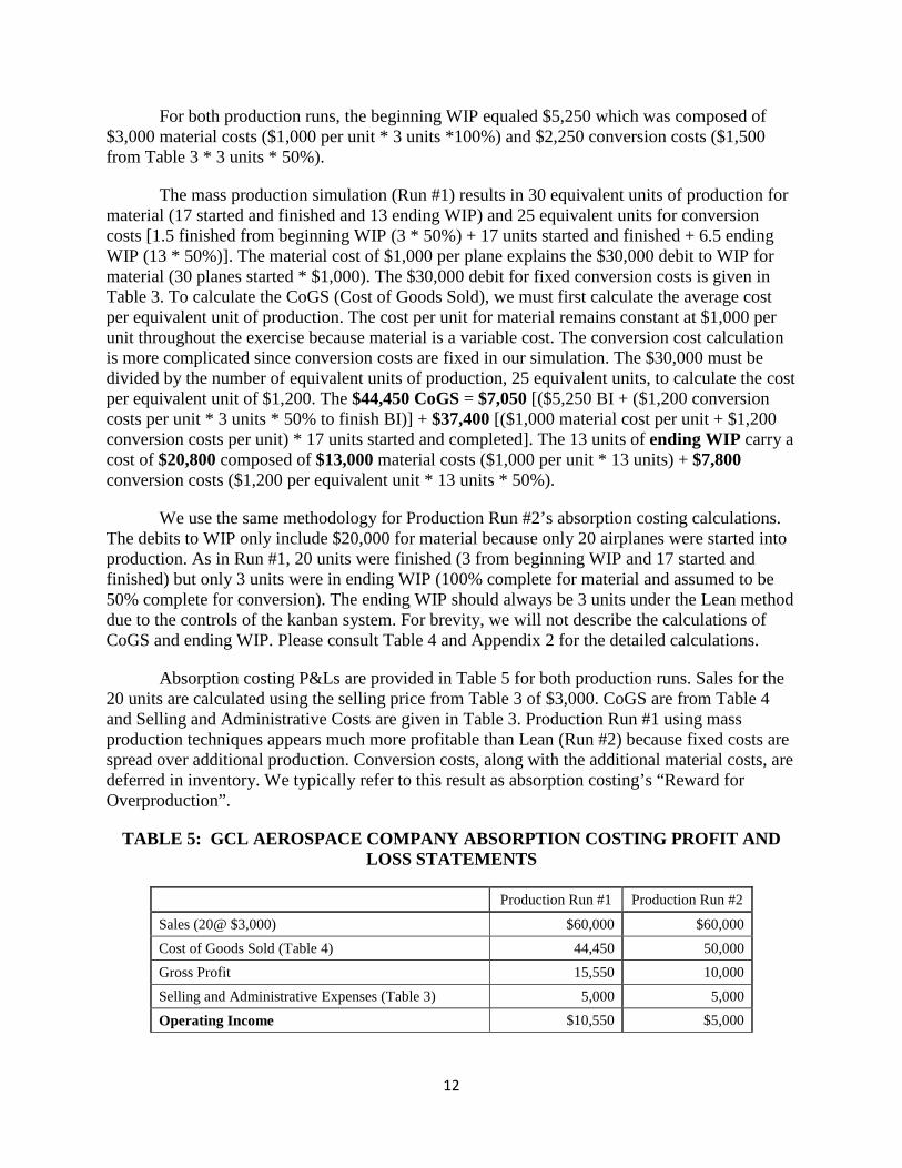
For both production runs, the beginning WIP equaled $5,250 which was composed of $3,000 material costs ($1,000 per unit * 3 units *100%) and $2,250 conversion costs ($1,500 from Table 3 * 3 units * 50%).
The mass production simulation (Run #1) results in 30 equivalent units of production for material (17 started and finished and 13 ending WIP) and 25 equivalent units for conversion costs [1.5 finished from beginning WIP (3 * 50%) + 17 units started and finished + 6.5 ending WIP (13 * 50%)]. The material cost of $1,000 per plane explains the $30,000 debit to WIP for material (30 planes started * $1,000). The $30,000 debit for fixed conversion costs is given in Table 3. To calculate the CoGS (Cost of Goods Sold), we must first calculate the average cost per equivalent unit of production. The cost per unit for material remains constant at $1,000 per unit throughout the exercise because material is a variable cost. The conversion cost calculation is more complicated since conversion costs are fixed in our simulation. The $30,000 must be divided by the number of equivalent units of production, 25 equivalent units, to calculate the cost per equivalent unit of $1,200. The $44,450 CoGS = $7,050 [($5,250 BI + ($1,200 conversion costs per unit * 3 units * 50% to finish BI)] + $37,400 [($1,000 material cost per unit + $1,200 conversion costs per unit) * 17 units started and completed]. The 13 units of ending WIP carry a cost of $20,800 composed of $13,000 material costs ($1,000 per unit * 13 units) + $7,800 conversion costs ($1,200 per equivalent unit * 13 units * 50%).
We use the same methodology for Production Run #2’s absorption costing calculations. The debits to WIP only include $20,000 for material because only 20 airplanes were started into production. As in Run #1, 20 units were finished (3 from beginning WIP and 17 started and finished) but only 3 units were in ending WIP (100% complete for material and assumed to be 50% complete for conversion). The ending WIP should always be 3 units under the Lean method due to the controls of the kanban system. For brevity, we will not describe the calculations of CoGS and ending WIP. Please consult Table 4 and Appendix 2 for the detailed calculations.
Absorption costing P&Ls are provided in Table 5 for both production runs. Sales for the 20 units are calculated using the selling price from Table 3 of $3,000. CoGS are from Table 4 and Selling and Administrative Costs are given in Table 3. Production Run #1 using mass production techniques appears much more profitable than Lean (Run #2) because fixed costs are spread over additional production. Conversion costs, along with the additional material costs, are deferred in inventory. We typically refer to this result as absorption costing’s “Reward for Overproduction”.
TABLE 5: GCL AEROSPACE COMPANY ABSORPTION COSTING PROFIT AND LOSS STATEMENTS
Production Run #1 Production Run #2
Sales (20@ $3,000) $60,000 $60,000 Cost of Goods Sold (Table 4) 44,450 50,000 Gross Profit 15,550 10,000 Selling and Administrative Expenses (Table 3) 5,000 5,000
Operating Income $10,550 $5,000

13
If one were to look at cash flow from operations, Production Run #1 would look less favorable. In Run #1 an additional 10 pieces of raw material were used (30 planes started in Run #1 versus 20 planes in Run #2). The additional consumption of raw materials will result in an additional cash outflow of $10,000 (10 extra pieces of raw material @ $1,000 per unit). This difference in cash flows is an important part of the exercise. Later, the instructor can point out that Lean Accounting’s Value Stream P&Ls more closely mirror the cash flows.
Product Run #1 would also incur costs to store and manage the additional inventory. These costs, including the costs of capital, are not reflected in this exercise. These very real additional costs should be discussed.
Lean Accounting / Value Stream Costing
Lean organizations adopt a “value stream” organizational structure. Each value stream consists of all the resources dedicated to produce similarly manufactured products or similarly provided services. In our example, we have only one value stream. We, however, do not assume that all of the resource costs are dedicated to this value stream. Some costs are primarily for sustaining the facility and some costs may be corporate overhead. Both are labeled “sustaining costs” and deducted “below the line” in Table 6 because they are not controllable by value stream personnel. The Value Steam P&L typically includes the costs of resources directly attributable to the value stream (i.e. controllable) and does not include costs that have to be allocated (i.e. not controllable). This is usually not a problem since Lean organizations favor dedicating resources, both people and equipment, to value streams. One common exception to the no-allocation rule is facilities costs. These costs are usually allocated on a basis of the square feet of floor space consumed by the value stream and does not include the cost of unused square footage. This allocation serves to provide an incentive for the value stream to reduce the size of their footprint.

14
TABLE 6: GCL AEROSPACE COMPANY AIRPLANE VALUE STREAM PROFIT AND LOSS STATEMENTS
Production Run #1
Production Run #2
Sales $60,000 $60,000 Value Stream Costs: Purchases 30,000 20,000 Payroll & Fringes 7,500 7,500 Supplies 500 500 Equipment Depreciation 8,000 8,000 Facility Costs 10,000 10,000 Total Value Stream Costs $56,000 $46,000
Value Stream Profit $4,000 $14,000 Percent of Sales 6.67% 23.33% Less: Sustaining Costs $9,000 $9,000 Inventory Increase/(Decrease) $15,550 $0
GAAP Operating Income $10,550 $5,000
Table 6 includes the Lean Accounting calculation of value stream profit and business unit operating income for both production runs. Note that the value stream profit is much lower for Production Run #1 than #2. This is contrary to GAAP absorption costing which rewards overproduction. Lean Accounting uses what is commonly referred to as “value steam costing” which focuses on profitability of a value stream instead of a particular product or job.
We assume in our example, for simplicity, all raw materials used are purchased in the current period. Value stream costing recognizes costs when incurred and does not defer costs in inventory. Any additional costs incurred to produce more than what is needed to satisfy customer demand is expensed immediately. Therefore, material costs are $10,000 ($30,000 - $20,000) higher for Run #1 because of the additional production (30 units started for Run #1 versus 20 units started for Run #2 with $1,000 material cost per plane). Lean Accounting not only does not reward overproduction, it penalizes it by recognizing the additional cash outlay for materials.
Lean Accounting, therefore, also encourages the conservation of resources. Lean Accounting will reward value streams for reducing inventory levels. To reduce inventory levels, sales must exceed production. In this case, sales are booked for units sold out of inventory with no incremental costs being incurred and booked. The aforementioned attributes of value stream costing means Lean Accounting tracks more closely with operating cash flows than does absorption costing.

15
The breakdown of conversion costs and S&A costs to the various line items on the Value Stream P&L is given in Table 2. The Value Steam P&L can be reconciled to absorption operating income by subtracting the non-allocated sustaining costs (including non-allocated facility costs) and by either adding an increase in inventory or subtracting a decrease in inventory. These adjustments take place below the value stream profit line or preferably on an additional report.
FURTHER DISCUSSION OF FINANCIAL RESULTS
Below are some of the issues that we recommend discussing with students if they were not covered during the preparation of the financial results.
Presentation
Is absorption costing or Lean Accounting better for decision making? In Lean Accounting the financial results are presented quite differently from absorption costing. The Lean Accounting presentation of the financial statements helps employees not familiar with financial statements better understand the financial situation in their value stream. Most costs shown in the P&L are incurred in that period and directly attributable to the value stream. This is possible because management has made the decision to reorganize around value streams. Lean organizations are decentralized with management pushing many decisions down to the value stream level. Absorption costing allocates current period costs to both the cost of goods sold (where it is combined with beginning inventory costs) and to ending inventory. Manufacturing costs are reflected only in the one line, “cost of goods sold”. This presentation lacks sufficient detail for decision making, whereas, the Lean Accounting P&L contains the detail.
Overproduction / Cash Flows
Does absorption costing or Lean Accounting better reflect cash flow from operations? As described earlier when production exceeds sales, absorption costing allocates the fixed costs over more production, thus lowering the average cost per unit produced. This has the effect of lowering costs of goods sold and increasing profits even though additional cash has been expended to purchase materials and cover other incremental costs of production. Lean Accounting does not suffer from this affliction. In fact, Lean Accounting will penalize overproduction as additional resources (e.g. material and other incremental costs) are expended without increasing sales. In Lean Accounting, costs are not deferred into inventory. Lean Accounting will also reward the organization who reduces inventory levels. There are additional revenues without incremental production costs in this case. The Lean Accounting P&L more closely reflects operating cash flows than traditional accrual basis GAAP income statements.
Idle Time
Does the idle time in the non-constrained work centers in Production Run #2 adversely affect the “true” financial results? Absorption costing results seem to indicate that the idle time increases costs and lowers profits. We know, however, that both runs produce the same number of finished units in the same length of time. Theory of Constraints and Lean Philosophy tell us that additional WIP is waste. Only the Lean Accounting P&L recognizes that idle time in some

16
work centers is much better than additional WIP impeding flow through the entire value stream. Only the Lean Accounting P&L promotes the conservation of resources (material in our example).
CONCLUSION
By focusing on value streams instead of production jobs, Lean Accounting provides more easily understood and useful information for value stream personnel and business-unit managers.
ADDITIONAL NOTE TO THE INSTRUCTOR
We use process costing in this example because of its ability to simplify the calculations for partially completed WIP. The authors discuss job costing and standard costing during the simulation with its detailed tracking of inventory movement and labor costs. We state that job costing requires large numbers of transactions while often providing incentives counter to the Lean Philosophy. As an example, laborers and management often optimize efficiency variances (standard cost systems) and absorption credit. This optimization done at the work center level is an additional factor causing overproduction. Lean Accounting typically involves shutting off product cost calculators like job costing.
Students may correctly point out that without job costing the accounting department will have trouble valuing inventory. Lean organizations, recognizing that inventory is waste and a barrier to flow, will reduce the amount carried. With the lower inventory levels, the valuation is done using simple estimation techniques consistent with process costing methodology. Any valuation errors are typically very small relative to materiality limits.

17
WORKS CITED
Billington, P. J. (2004). A Classroom Exercise to Illustrate Manufacturing Pull Concepts. Decision Sciences Journal of Innovative Education, 2(1), 71-76.
DeBusk, G. K., & DeBusk, C. (2010). Characteristics of Successful Lean Six Sigma Organizations. Cost Management, 24(1), 5-10.
DeBusk, G. K., & DeBusk, C. (2011). Combining Hoshin Planning with the Balanced Scorecard to Achieve Breakthrough Results in Lean Six Sigma Organizations. Balanced Scorecard Report, 13(6), 7-10.
DeBusk, G. K., & DeBusk, C. (2011). Has Your Accounting Department Evolved? Accounting and the Use of Lean Six Sigma. Cost Management, 25(3), 15-19.

18
APPENDIX 1: GCL AEROSPACE COMPANY PROCESS COST WORKSHEET FOR PRODUCTION RUN #1
Equivalent Units
Physical Units
Direct Materials Conversion
Units to be accounted for:
Beginning WIP inventory 3
Units started this period 30 Total units to be accounted for 33
Units accounted for:
Beginning WIP inventory 3 0 1.5
Started and completed 17 17 17
Total completed and transferred out 20 17 18.5
Units in ending WIP inventory 13 13 6.5
Total units accounted for 33 30 25
Costs
Total
Direct Materials Conversion
Costs to be accounted for:
Costs in beginning WIP inventory $5,250 $3,000 $2,250
Current period costs 60,000 30,000 30,000
Total costs to be accounted for $65,250 $33,000 $32,250 Costs per equivalent unit
$1,000 $1,200
Costs accounted for:
Costs from beginning WIP inventory $5,250 $3,000 $2,250
Current costs to complete beginning WIP 1,800 0 1,800
Costs of units started and completed 37,400 17,000 20,400
Total costs transferred out 44,450 20,000 24,450
Costs of ending WIP inventory 20,800 13,000 7,800
Total costs accounted for $65,250 $33,000 $32,250

19
APPENDIX 2: GCL AEROSPACE COMPANY PROCESS COST WORKSHEET FOR PRODUCTION RUN #2
Equivalent Units
Physical Units
Direct Materials Conversion
Units to be accounted for:
Beginning WIP inventory 3
Units started this period 20 Total units to be accounted for 23
Units accounted for:
Beginning WIP inventory 3 0 1.5
Started and completed 17 17 17
Total completed and transferred out 20 17 18.5
Units in ending WIP inventory 3 3 1.5
Total units accounted for 23 20 20
Costs
Total
Direct Materials Conversion
Costs to be accounted for:
Costs in beginning WIP inventory $5,250 $3,000 $2,250
Current period costs 50,000 20,000 30,000
Total costs to be accounted for $55,250 $23,000 32,250 Costs per equivalent unit
$1,000 $1,500
Costs accounted for:
Costs from beginning WIP inventory $5,250 $3,000 $2,250
Current costs to complete beginning WIP 2,250 0 2,250
Costs of units started and completed 42,500 17,000 25,500
Total costs transferred out 50,000 20,000 30,000
Costs of ending WIP inventory 5,250 3,000 2,250
Total costs accounted for $55,250 $23,000 $32,250

1
The Personal Budget: A Value Added Tool for the Managerial Accounting Class
Raymond J Elson, DBA, CPA
Professor of Accounting Valdosta State University
Langdale College of Business 1500 N Patterson St Valdosta, GA 31698
229-219-1214 (office) [email protected]

2
The Personal Budget: A Value Added Tool for the Managerial Accounting Class
ABSTRACT
Students often need activities to help them process and understand accounting concepts. This is especially true for managerial accounting, a course offered to accounting and non-accounting (including non-business) majors. One such activity is the personal budget. It’s a simple value-added activity that is used to demonstrate key course concepts such as cost behavior, profit planning, and variance analysis in the managerial accounting course. This paper describes the personal budget exercise and provides accounting instructors with a template for use in their own course.
INTRODUCTION
Educators are using non-traditional learning tools to engage students in the classroom. Such tools ranging from crossword puzzles to clickers are meant to provide students with more classroom interaction. While these tools are effective, they may not help students connect the various concepts discussed in the courses.
Managerial accounting, a course offered to accounting and non-accounting (including non-business) majors in business schools has its own unique challenges. Financial accounting, often the first accounting course, has a number of subject matter or concepts that ultimately culminate in the preparation of financial statements. However, managerial accounting concepts are often disconnected and do not provide students with a comprehensive view of the subject matter. So each instructor has the latitude to present these series of concepts in a matter that is conducive to their teaching style.
However, students do not often understand the interrelationship between these concepts or topics. Also, unlike the preparation of financial statements, managerial accounting students are often looking for activities that can help them process and understand accounting concepts. One such activity is the personal budget.
THE PERSONAL BUDGET
The personal budget is a value added exercise that is created from each student’s experience. It is a simple tool, unique to each student, and demonstrates key course concepts such as cost behavior, profit planning, and variance analysis from the managerial accounting course. As such the learning outcomes are to enable students to:
a) Understand cost behavior (fixed versus variable costs) b) Understand the importance of a budget (profit planning) c) Determine the importance of variance analysis

3
These concepts are connected since there are important in managing any business. This relationship is shown below.
The personal budget exercise is used over multiple semesters and years by the author. It could be adopted and used by instructors in other classes such as an introduction to business course, cost accounting, and personal finance.
The Instructions
The course syllabi provide students with guidelines on the preparation of the personal budget as well as a template for its preparation. A copy of the personal budget instructions is provided in Appendix A.
During the first month of the semester (e.g. August), students are asked to prepare a detailed budget for the following month (e.g., September). The budget must separate income from expenses and categorize expenses by their behavior (i.e., fixed or variable). Mixed costs are excluded to help simplify the project. During the budgeted month (i.e., September), students track the income received and the use of those funds. In the third month (e.g., October), students provided a comparison of the budget versus actual amounts, and explanations for all variances above an established threshold such as +/- 10%.
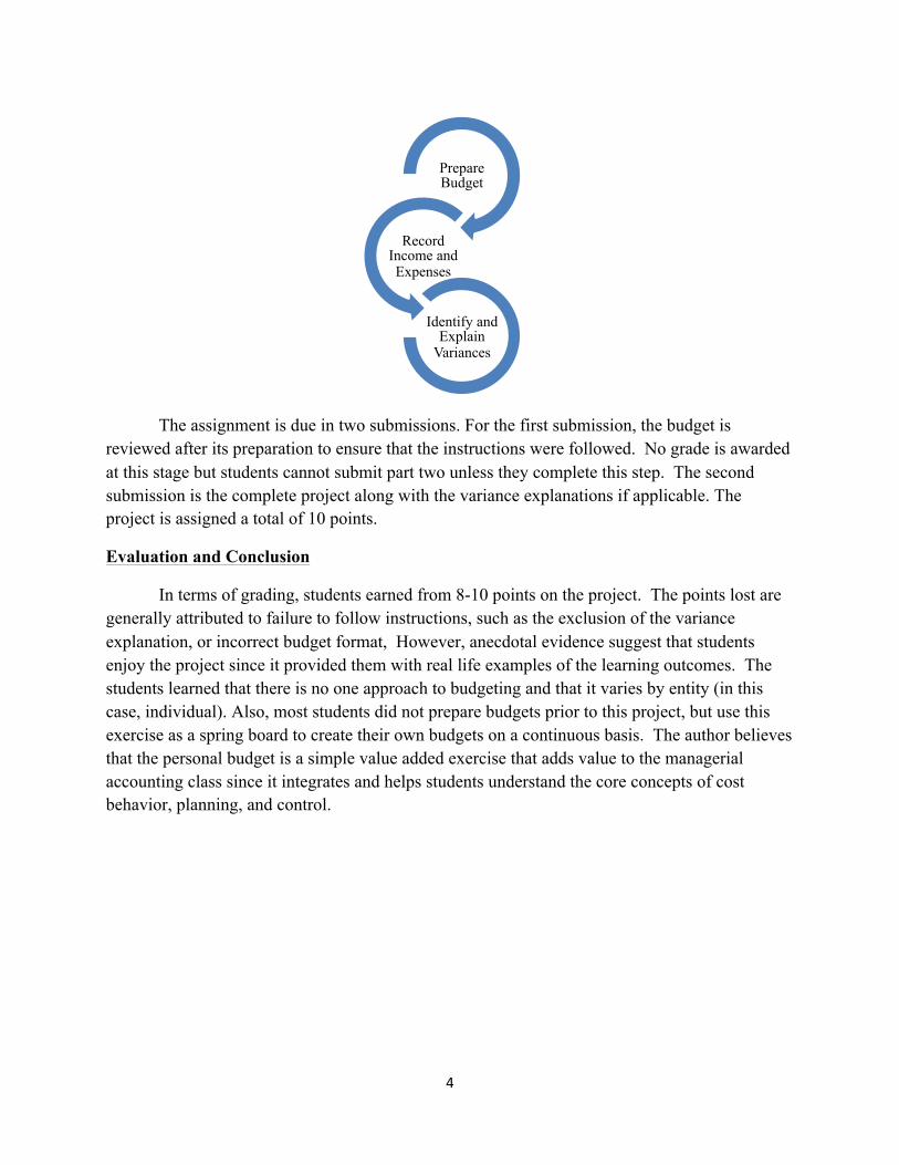
The steps in the process are shown below:
Cost Analysis (Behavior)
Planning (Budget)
Control (Variance Analysis)
4
The assignment is due in two submissions. For the first submission, the budget is reviewed after its preparation to ensure that the instructions were followed. No grade is awarded at this stage but students cannot submit part two unless they complete this step. The second submission is the complete project along with the variance explanations if applicable. The project is assigned a total of 10 points.
Evaluation and Conclusion
In terms of grading, students earned from 8-10 points on the project. The points lost are generally attributed to failure to follow instructions, such as the exclusion of the variance explanation, or incorrect budget format, However, anecdotal evidence suggest that students enjoy the project since it provided them with real life examples of the learning outcomes. The students learned that there is no one approach to budgeting and that it varies by entity (in this case, individual). Also, most students did not prepare budgets prior to this project, but use this exercise as a spring board to create their own budgets on a continuous basis. The author believes that the personal budget is a simple value added exercise that adds value to the managerial accounting class since it integrates and helps students understand the core concepts of cost behavior, planning, and control.
Prepare Budget
Record Income and Expenses
Identify and Explain
Variances

5
Appendix A: ACCT 2XXX - Principles of Accounting II
Personal Budget Assignment Value = 10 points
Objective: To provide students with the opportunity to apply concepts discuss in the course to their personal situations. Instructions:
1. During the month of August (Month #1), you will prepare a budget of your anticipated income and expenses for the month of September. You should use Excel or similar product for this project. The spreadsheet should be formal and prepared as shown on the following page. At a minimum, your budget should identify the following items and your expenses should be classified by their behavior (i.e., fixed or variable).
Income (broken down by sources), Expenses (including) Rent Utilities Clothing Cell phone payments Credit card payments Auto expenses (other than gas) Gas Entertainment Groceries
Try not to use “other” or “miscellaneous” in your budget 2. During the month of September (Month #2), you will monitor or track the actual income received
and expenses incurred or paid for the categories identified in your budget. At the end of September, you will tabulate the total of each income and expense item included in your budget.
3. In early October (Month #3), you will compare the actual amounts to the budget amounts and identify the difference or variance between the amounts. You will provide an explanation for any variance that is 5% or greater than the budgeted amount.
Deliverables
1. A copy of your budget is due on Date #1, e.g., September 4th (this is non-graded, serves as a progress report)
2. The completed project is due on Date #2, e.g., October 18th. You cannot complete deliverable #2 if you failed to turn in deliverable #1.
Important: Hand written and late projects are not accepted for grading. A project is considered late if it is
submitted later than 5 minutes from the beginning of the class period.

6
Appendix A (cont’d) ACCT 2XXX - Principles of Accounting II
Personal Budget (cont’d) Assignment Value = 10 points
Name Personal Budget
For the month of September 201X
Variance Category Budget Actual Dollar Percentage

LEARNING THE ACCOUNTING FOR ACCOUNTS RECEIVABLE AND BAD DEBTS:
AN INTERACTIVE APPROACH
Angela Hwang (corresponding author) Professor of Accounting
Eastern Michigan University Department of Accounting and Finance
406 Owen Building Ypsilanti, MI 48197 [email protected]
Andrew Romanowski, CPA Baker Tilly Virchow Krause, LLP
Daniel R. Brickner Professor of Accounting
Eastern Michigan University Department of Accounting and Finance
406 Owen Building Ypsilanti, MI 48197

1
LEARNING THE ACCOUNTING FOR ACCOUNTS RECEIVABLE AND BAD DEBTS: AN INTERACTIVE APPROACH
INTRODUCTION
Students are often confused by the impact and timing of recording transactions and events that affect the net realizable value of accounts receivable and bad debts. This instructional resource uses a comprehensive problem to illustrate an interactive approach of teaching/learning concepts related to accounting for accounts receivable and bad debts in a principles of financial accounting course.
The problem contains background information about a company followed by a set of transactions/events over two accounting periods. Students are asked to record them on a spreadsheet that accompanies the problem by preparing all accounting entries in T-account format for a complete accounting cycle. This process helps students learn and develop critical-thinking skills by addressing the issues of uncollectible accounts on credit sales, explaining the concept of net realizable value of accounts receivable, identifying the reasons that bad debts are estimated, analyzing the appropriateness of the bad debt estimation in a changing economy, and examining the differences between the income statement and balance sheet approaches in estimating bad debts.
A downloadable spreadsheet is provided for use in conjunction with class discussion of
the problem, helping to facilitate an interactive and engaging presentation. A video clip for instructors is included to demonstrate the use of the interactive spreadsheet to show/hide the numbers (with built-in formula) for class discussion. A clip for students is also available as a tutorial or for after-class review. Click the links below for the teaching aids: Worksheet/Solution https://www.dropbox.com/s/ik8w5tul912jde7/AR_Worksheet.xlsx Instructor video http://www.youtube.com/watch?v=_lSVcULwUQg Solution video http://www.youtube.com/watch?v=it5OMnKr8gg
BACKGROUND
ABC Fashion Company (ABC hereafter) is a retailer that sells a wide variety of different articles of clothing, from shirts to shoes. ABC is owned by Andrew and Betty Carlton, whose passions are in clothing design and retail, but not accounting. ABC currently generates all of its revenue through credit sales. Also, the allowance method is applied to account for bad debts by using credit sales to estimate the amount of accounts receivable that likely will be uncollectible.
On March 1, you are hired to manage the accounts receivable. On your first day, Andrew
Carlton greets you at the door and takes you to your office. He tells you that it is your responsibility to enter all of the transactions/events affecting accounts receivable, including adjusting and closing entries. As he is leaving, he starts mumbling additional information, and you barely have time to write it all down. Once he is gone you read your note, which contains the following information:

2
• $346,000 of retained earnings for ABC • $300,000 in cash • Total amount of $50,000 owed to them for prior sales • The balance in their allowance for bad debts is $4,000
You look down at your desk and are pleasantly surprised to find that you have been given a spreadsheet with all the necessary accounts. During March, the following transactions and events occurred.
[See Exhibit 1: Worksheet]
March Transactions/Events 3/5 ABC sells $120,000 worth of t-shirts to customers on credit.1 3/19 ABC receives $138,000 in cash from customers in payment for prior purchases. 3/22 You determine that the $7,000 balance owed by MC Jammer is uncollectible. 3/26 ABC sells $40,000 worth of hats to customers. No cash was received at the time the sales
took place. 3/31 The end-of-period bad debt adjustment is made; based on the company’s policy, the
adjustment is estimated to be 5% of sales for the period.
Requirements (March): The ABC owners approach you at the end of the month with a list of questions they want answered. 1. How are the journal entries recorded in the spreadsheet for March? 2. What is both the gross amount and the net realizable value of accounts receivable (NRV) for
ABC at the end of the month? Which of these two amounts is likely to be received in cash, and why?
3. Why is an estimated amount recorded for bad debt expense instead of an actual amount? 4. For the transactions that you recorded in March, which accounts would be closed at the end
of the month? Why are those accounts closed and the other accounts are not? What are the necessary closing entries?
5. Does ABC use the balance sheet approach or the income statement approach in estimating bad debt expense, and what is the difference between these methods?
April Transactions/Events: 4/3 You conclude that $4,000 owed by David Walker is uncollectible. 4/5 ABC sells $110,000 worth of clothes to customers on credit. 4/21 ABC receives $90,000 from customers for previous sales made on credit. 4/23 The XYZ Co. account was previously written-off as uncollectible, but ABC unexpectedly
receives a full payment of $3,000 from XYZ Co. 4/27 ABC sells $10,000 of shirts to Big Ben Clothing on credit. 4/28 You conclude that $21,000 owed by R. Logan is uncollectible. 4/30 The end-of-period bad debt adjustment is made, based again on 5% of sales for the
period.
1 To focus on transactions that affect accounts receivable, the entry to record cost of sales and inventory is omitted.

3
Requirements (April): To understand the effects on the financial statements, ABC’s owners ask even more questions of you at the end of April. 1. What is the beginning balance for each account on April 1st? Why do some accounts have a
balance and others do not? 2. What are the required journal entries for April, and what are the ending balances in each
account? 3. Based on the NRV of accounts receivable immediately before and after the transaction on
April 3rd, how is the NRV affected by the write-off? 4. What are both the purpose and the effects of the entries for the April 23rd transaction? 5. What is the NRV of accounts receivable on April 30th (after adjustments)? Is this likely to
occur? 6. What does the debit balance in the allowance for bad debts account indicate? 7. Does the percentage of sales rate being used to estimate bad debts appear appropriate? If you
believe it is not appropriate, propose a new rate and justify your suggestion. 8. If a new rate is implemented, what effect will this change have on prior financial statements? 9. The income statement approach was used to estimate bad debts, and it resulted in a debit
balance for the allowance account in the month of April. If the balance sheet approach was used for the bad debt adjustment, could that method have resulted in a debit balance for the allowance account at the end of the period?
LEARNING OBJECTIVES AND IMPLEMENTATION GUIDANCE
Overview There has been much discussion in recent years about the need for instructors to move
beyond sole reliance on the traditional lecture-based approach to accounting education and to employ pedagogical strategies so students become active and engaged learners (see Albrecht and Sack, 2000 and AAHE, 1998 for examples). We agree with that refrain, and have thus attempted to enhance student engagement and understanding related to the accounts receivable cycle, an area identified by the authors as one causing significant challenges and difficulties for students in an introductory financial accounting course. To meet this end, we created this instructional material, which is presented in the form of a comprehensive problem related to accounts receivable.
An interactive spreadsheet is designed as a tool to aid in the learning for introductory
accounting students. Each row corresponds to a specific transaction, ordered chronologically as presented in the problem. The first column provides the details for each event/transaction that occurs, and the next column provides the specific amount for the transaction. This reference column allows instructors to customize the transactions, as all entries are linked with formulas to the proper reference column amount so dollar amounts can be easily changed by the instructor for illustrative purposes. Also, all the calculations throughout the spreadsheet (for net realizable value and the ending account balances) are built in with formulas that will auto-fill upon changing numbers in the reference column as shown in Exhibit 2. The rest of the columns are T-accounts for each respective account affected in the events that occur throughout the problem. This design allows students to utilize T-accounts and also visually see the specific debit and credit entries that correspond to each transaction.
4
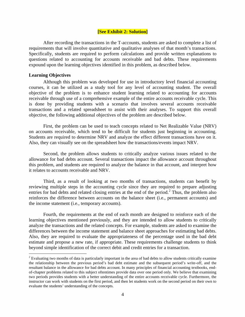
[See Exhibit 2: Solution]
After recording the transactions in the T-accounts, students are asked to complete a list of requirements that will involve quantitative and qualitative analyses of that month’s transactions. Specifically, students are required to perform calculations and provide written explanations to questions related to accounting for accounts receivable and bad debts. These requirements expound upon the learning objectives identified in this problem, as described below.
Learning Objectives Although this problem was developed for use in introductory level financial accounting
courses, it can be utilized as a study tool for any level of accounting student. The overall objective of the problem is to enhance student learning related to accounting for accounts receivable through use of a comprehensive example of the entire accounts receivable cycle. This is done by providing students with a scenario that involves several accounts receivable transactions and a related spreadsheet to assist with their analyses. To support this overall objective, the following additional objectives of the problem are described below.
First, the problem can be used to teach concepts related to Net Realizable Value (NRV)
on accounts receivable, which tend to be difficult for students just beginning in accounting. Students are required to determine NRV and analyze the effect different transactions have on it. Also, they can visually see on the spreadsheet how the transactions/events impact NRV.
Second, the problem allows students to critically analyze various issues related to the
allowance for bad debts account. Several transactions impact the allowance account throughout this problem, and students are required to analyze the balance in that account, and interpret how it relates to accounts receivable and NRV.
Third, as a result of looking at two months of transactions, students can benefit by
reviewing multiple steps in the accounting cycle since they are required to prepare adjusting entries for bad debts and related closing entries at the end of the period.2 Thus, the problem also reinforces the difference between accounts on the balance sheet (i.e., permanent accounts) and the income statement (i.e., temporary accounts).
Fourth, the requirements at the end of each month are designed to reinforce each of the
learning objectives mentioned previously, and they are intended to allow students to critically analyze the transactions and the related concepts. For example, students are asked to examine the differences between the income statement and balance sheet approaches for estimating bad debts. Also, they are required to evaluate the appropriateness of the percentage used in the bad debt estimate and propose a new rate, if appropriate. These requirements challenge students to think beyond simple identification of the correct debit and credit entries for a transaction. 2 Evaluating two months of data is particularly important in the area of bad debts to allow students critically examine the relationship between the previous period’s bad debt estimate and the subsequent period’s write-off, and the resultant balance in the allowance for bad debts account. In many principles of financial accounting textbooks, end-of-chapter problems related to this subject oftentimes provide data over one period only. We believe that examining two periods provides students with a better understanding of the entire accounts receivable cycle. Furthermore, the instructor can work with students on the first period, and then let students work on the second period on their own to evaluate the students’ understanding of the concepts.
5
Implementation Guidance Differences between March and April Transactions
The problem contains transactions that occur over a period of two months. The set of transactions for March are relatively easier than April. Depending on where each class is as a whole, the suggested method is to review the March transactions together as a class, engaging students in discussion over each transaction and the requirements. The instructor can then let the students attempt April’s requirements on their own (either individually or in small groups). The March transactions will serve as a tool to guide them through the requirements for April. After the students have attempted the April transactions, the instructor can discuss the answers with them as a class.
Use during a Classroom Lecture
An appealing attribute of this exercise is that it allows the instructor to engage the students to critically think about each different event/transaction and evaluate how each account would be impacted. This approach should prove helpful for instructors in diagnosing areas or concepts about which students are struggling. When the instructor is satisfied with the discussion regarding that transaction, he/she can reveal the solution. This process can then be repeated throughout all of the transactions. The spreadsheet that accompanies the problem contains two worksheets – one for students to complete the problem and the other, which contains the transactions’ solutions, for instructors. The interactive spreadsheets allow the instructor to customize them, and thus the problem, for their specific class needs.3
Use as a Self-study Aid
The problem can also be given to students as an individual assignment that can be completed on their own. After allowing students to work through it themselves, the instructor can provide them with the solutions to the transactions or direct students to watch the demo video. They can utilize this as a self-study aid that could serve as a valuable reference in preparing for an examination.
Classroom Experience
This problem has been used by two instructors in multiple sections of principles of financial accounting courses (both undergraduate and graduate) over the last two years. Since its use in the classroom, the instructors have observed apparent increased understanding of the related concepts by their students. These outcomes have been anecdotally perceived in both increased student participation and engagement during course lectures on the topic and improved performance on related examination questions. As stated above, it appears that the use of the spreadsheet provided with the problem materials enhances the classroom discussion and student understanding of the material.
The problem is relatively easy to implement and offers flexibility for the instructor to use
in class as an illustrative problem to supplement a related lecture, as a stand-alone assignment, or
3 The authors use the spreadsheet to reveal the transactions’ solution in class. We initially conceal the answer for each requirement/transaction (row) by having the answers in white font so they are not visible to the students. After class discussion related to the transaction, we change the font color for the row in question so the correct answer is revealed. We have found that this interactive approach to revealing the solutions appears to improve both class discussion and student engagement, thus enhancing the case’s effectiveness as a teaching tool.

6
a combination of these two. The authors are able to cover this problem in its entirety in about thirty minutes of class time. However, instructors who assign this to students as a stand-alone assignment should anticipate it taking approximately one hour for students to complete on their own.
REFERENCES
Albrecht, W. S., and R. J. Sack. 2000. Accounting Education: Charting the Course through a Perilous Future. Accounting Education Series, Vol. 16. Sarasota, FL: American Accounting Association.
American Association for Higher Education. 1998. Learning by Doing: Concepts and Models for
Service-Learning in Accounting. Washington, D.C.: AAHE.

7
TEACHING NOTES
Requirements (March): 1. This requirement is designed as a review of journalizing in the accounts receivable cycle.
Students should be able to identify the proper debit and credit accounts for each event. See Exhibit 2 for the solution.
2. This requirement is designed to teach the students the concept and definition of Net Realizable Value (NRV) on accounts receivable. Students should note that NRV is the amount of accounts receivable that is likely to be realized (received) in cash. As indicated in the spreadsheet solution, students should compute a NRV for accounts receivable as of March 31st of $60,000, computed as follows:
NRV = Gross A/R (Debit balance) – Allowance
(Credit balance) $60,000 = $65,000 – $5,000
3. This requirement requires students to analyze why bad debts are estimated under the
allowance method. The instructor can emphasize that the allowance method requires recognition of bad debt expense to apply the matching principle that underlies the preparation of the income statement. Specifically, if the sales revenue was recorded in one period, all related expenses, including bad debt expense, should be recorded in the same accounting period. The instructor could further elaborate about the importance of evaluating credit worthiness of customers and emphasize that companies are oftentimes willing to assume some level of risk of not getting paid (credit risk) because losses from bad debts could be more than offset by increased sales and profits on other credit sales that ultimately are realized in cash.
4. The objective of this requirement is to illustrate the difference between accounts on the income statement (temporary accounts) and accounts on the balance sheet (permanent accounts). The instructor could emphasize that since both sales and bad debt expense are found on the income statement, they both would be closed so the company can begin the following period with $0 balances for those accounts. The spreadsheet that accompanies this problem provides the closing entries in T-account form.
5. This requirement is designed to help students identify and understand the differences
between the balance sheet and income statement approaches in accounting for bad debts under an allowance method. Since ABC estimates their bad debts expense using a percentage of credit sales, they use the income statement approach (i.e., they use one income statement account, sales, to estimate another income statement account, bad debt expense). If the balance sheet method was used, the company would use a percentage of accounts receivable to estimate the ending balance for the allowance for bad debts account (i.e., one balance sheet account, accounts receivable, is used to estimate the ending balance of another balance sheet account, allowance for bad debts). The instructor could also explain that companies using this approach oftentimes use different percentages for individual accounts receivable balances based on the age of those balances.

8
Requirements (April): 1. This requirement is designed to illustrate the effect of the previous period’s closing entries on
the current period’s beginning account balances. It should be noted to students that only balance sheet accounts (i.e., permanent accounts) have opening balances, and that temporary accounts begin each period with $0 balances since they were closed at the end of the previous accounting period. See Exhibit 2 for the solution.
2. See Exhibit 2.
3. This requirement again addresses the concept of NRV and how it is impacted by the write-off of an account under the allowance method. The instructor can explain that writing off an account as uncollectible occurs after efforts to collect have failed. Under the allowance method, bad debt expense is never affected when an account is written off. In the related journal entry, the individual account receivable is taken off of the books through a credit entry, and the allowance account is debited. When thinking in terms of NRV, the amount likely to be received will not be affected by the April 3rd transaction since the debits and credits simply negate each other. The calculations are provided below, and the supporting numbers can be found in the spreadsheet that accompanies this problem.
NRV = Gross A/R
(Debit balance) – Allowance (Credit balance)
Before the April 3rd entry $60,000 = $65,000 – $5,000 After the April 3rd entry $60,000 = $61,000 – $1,000
4. There will be circumstances in which cash is collected on an account that was previously deemed to be uncollectible. In order to properly account for this situation, two entries typically are made. The first entry reverses the entry that was recorded when the account was previously written off, essentially re-instating the account back on the books as shown below.
Accounts receivable XXX
Allowance for bad debts XXX
The second entry is accounted for the same way as any other receipt of cash on account. There are no income effects from this situation, as all affected accounts are assets or a contra asset. Also, total assets remain unchanged as a result of these entries.
Cash XXX
Accounts receivable XXX
5. The supporting numbers in the spreadsheet indicate that the NRV of accounts receivable on April 30th is $81,000, computed as follows:
NRV = Gross A/R (Debit balance) + Allowance
(Debit balance) $81,000 = $70,000 + $11,000

9
This requirement is crucial to the learning objectives in this problem. It was developed to allow students to critically think about the concept of NRV, and if the NRV on April 30th makes practical sense. It is important to point out to students that the NRV is greater than the total balance of accounts receivable. This DOES NOT MAKE LOGICAL SENSE!!! It is illogical to believe that ABC will collect more than the current balance of accounts receivable. Another way of expressing this is that ABC will receive more than they expect to collect. This situation indicates that a new rate should be proposed. Determining an appropriate new rate is the objective of requirement #8.
6. Since it is a contra asset, one would expect the allowance for bad debts account to have a credit balance to offset accounts receivable. When there is a debit balance in the allowance account, it indicates that the actual amount of write-offs for uncollectible accounts was greater than the previous estimate for uncollectible accounts. This implies that both the allowance account and bad debt expense were understated, leading to an overstated NRV and net income, respectively.
7. This question relates to requirements #5 through #7 and builds on them by reinforcing the concept that the recorded amount for bad debt expense is based on an ESTIMATE. This question is designed to allow students to critically analyze if the current rate for estimating bad debts needs to be adjusted. Since the amount of write-offs in April exceeded the existing balance in the allowance for bad debts account, it would appear that ABC needs to increase their current estimated rate. In order to demonstrate to students how a new proposed rate can be determined, the instructor can propose that they take the amount written off as uncollectible in April, and divide it by the previous month’s sales amount, as shown below.
Proposed rate calculation: Amount written off in April $25,000 = 16% Total credit sales in March $160,000
8. This question is designed to reinforce the fact that any change in an estimate (which would
occur if a new rate is used) is treated prospectively and would not require any restatement of financial statements in prior periods. However, if the change in rate results in a material effect on the financial statements, disclosure of the change should be provided in the footnotes to the financial statements.
9. This question is designed for students to consider further the differences between the balance sheet and the income statement approaches. It requires them to think critically about the journal entry for bad debt expense and how it impacts the allowance for bad debts account. In the adjusting entry for bad debt expense, the accounts debited and credited would be the same under both the balance sheet and income statement methods, as shown below.
Bad debt expense XXX
Allowance for bad debts XXX The difference in the journal entries between the balance sheet and income statement approaches is simply the dollar amount in the adjusting entry and how that dollar amount is

10
determined. Students should note that under the balance sheet approach, it is the ending balance of the allowance for bad debts account that is determined, and that ending balance appears on the credit side of that account. Thus, it is impossible for that account to end the period with a debit balance using that approach. Unlike the balance sheet approach, the income statement approach does not take into account the existing balance in the allowance for bad debts account, thus making it possible for that account to end a period with a debit balance.
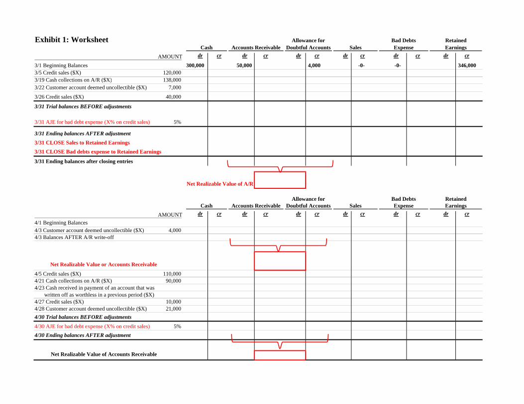
Exhibit 1: Worksheet Allowance for Bad Debts RetainedCash Accounts Receivable Doubtful Accounts Sales Expense Earnings
AMOUNT dr cr dr cr dr cr dr cr dr cr dr cr
3/1 Beginning Balances 300,000 50,000 4,000 -0- -0- 346,0003/5 Credit sales ($X) 120,000 120,000 120,0003/19 Cash collections on A/R ($X) 138,000 138,000 138,0003/22 Customer account deemed uncollectible ($X) 7,000 7,000 7,000
3/26 Credit sales ($X) 40,000 40,000 40,000
3/31 Trial balances BEFORE adjustments 438,000 65,000 3,000 160,000 -0- 346,000
3/31 AJE for bad debt expense (X% on credit sales) 5% 8,000 8,000
3/31 Ending balances AFTER adjustment 438,000 65,000 5,000 160,000 8,000 346,0003/31 CLOSE Sales to Retained Earnings ###### 160,000
3/31 CLOSE Bad debts expense to Retained Earnings 8,000 8,000
3/31 Ending balances after closing entries 438,000 65,000 5,000 -0- -0- 498,000
Net Realizable Value of A/R 60,000
Allowance for Bad Debts RetainedCash Accounts Receivable Doubtful Accounts Sales Expense Earnings
AMOUNT dr cr dr cr dr cr dr cr dr cr dr cr4/1 Beginning Balances 438,000 65,000 5,000 -0- -0- 498,0004/3 Customer account deemed uncollectible ($X) 4,000 4,000 4,000 4/3 Balances AFTER A/R write-off 61,000 1,000
Net Realizable Value or Accounts Receivable 60,0004/5 Credit sales ($X) 110,000 110,000 110,0004/21 Cash collections on A/R ($X) 90,000 90,000 90,0004/23 Cash received in payment of an account that was 3,000 3,000 written off as worthless in a previous period ($X) 3,000 3,000 3,0004/27 Credit sales ($X) 10,000 10,000 10,0004/28 Customer account deemed uncollectible ($X) 21,000 21,000 21,000 4/30 Trial balances BEFORE adjustments 531,000 70,000 17,000 120,000 -0- 498,000
4/30 AJE for bad debt expense (X% on credit sales) 5% 6,000 6,000 4/30 Ending balances AFTER adjustment 531,000 70,000 11,000 120,000 6,000 498,000
Net Realizable Value of Accounts Receivable 81,000
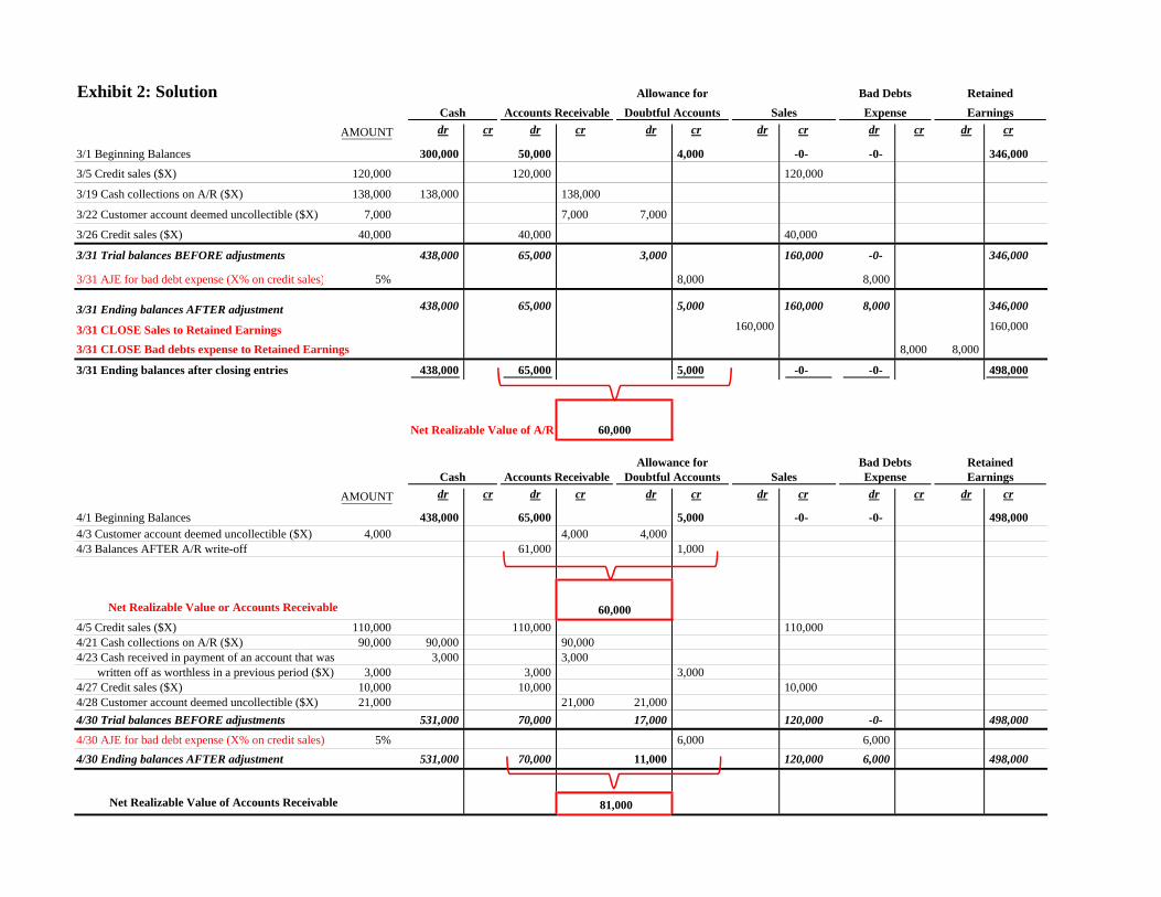
Exhibit 2: Solution Allowance for Bad Debts RetainedCash Accounts Receivable Doubtful Accounts Sales Expense Earnings
AMOUNT dr cr dr cr dr cr dr cr dr cr dr cr
3/1 Beginning Balances 300,000 50,000 4,000 -0- -0- 346,000
3/5 Credit sales ($X) 120,000 120,000 120,000
3/19 Cash collections on A/R ($X) 138,000 138,000 138,000
3/22 Customer account deemed uncollectible ($X) 7,000 7,000 7,000
3/26 Credit sales ($X) 40,000 40,000 40,000
3/31 Trial balances BEFORE adjustments 438,000 65,000 3,000 160,000 -0- 346,000
3/31 AJE for bad debt expense (X% on credit sales) 5% 8,000 8,000
3/31 Ending balances AFTER adjustment 438,000 65,000 5,000 160,000 8,000 346,000
3/31 CLOSE Sales to Retained Earnings 160,000 160,000
3/31 CLOSE Bad debts expense to Retained Earnings 8,000 8,000
3/31 Ending balances after closing entries 438,000 65,000 5,000 -0- -0- 498,000
Net Realizable Value of A/R 60,000
Allowance for Bad Debts RetainedCash Accounts Receivable Doubtful Accounts Sales Expense Earnings
AMOUNT dr cr dr cr dr cr dr cr dr cr dr cr
4/1 Beginning Balances 438,000 65,000 5,000 -0- -0- 498,0004/3 Customer account deemed uncollectible ($X) 4,000 4,000 4,000 4/3 Balances AFTER A/R write-off 61,000 1,000
Net Realizable Value or Accounts Receivable 60,0004/5 Credit sales ($X) 110,000 110,000 110,0004/21 Cash collections on A/R ($X) 90,000 90,000 90,0004/23 Cash received in payment of an account that was 3,000 3,000 written off as worthless in a previous period ($X) 3,000 3,000 3,0004/27 Credit sales ($X) 10,000 10,000 10,0004/28 Customer account deemed uncollectible ($X) 21,000 21,000 21,000 4/30 Trial balances BEFORE adjustments 531,000 70,000 17,000 120,000 -0- 498,000
4/30 AJE for bad debt expense (X% on credit sales) 5% 6,000 6,000 4/30 Ending balances AFTER adjustment 531,000 70,000 11,000 120,000 6,000 498,000
Net Realizable Value of Accounts Receivable 81,000

Note to the instructor: Amounts in columns 'D-T' are currently displayed. To HIDE those numbers, change the text to white color. To SHOW them, change the text to a color other than white.
Exhibit 2: Solution Allowance for Bad Debts RetainedCash Accounts Receivable Doubtful Accounts Sales Expense Earnings Learning Objectives:
AMOUNT dr cr dr cr dr cr dr cr dr cr dr cr
3/1 Beginning Balances 300,000 50,000 4,000 -0- -0- 346,000 1. Life cycle of AR3/5 Credit sales ($X) 120,000 120,000 120,000 a. Credit sales3/19 Cash collections on A/R ($X) 138,000 138,000 138,000 b. Cash collection from AR3/22 Customer account deemed uncollectible ($X) 7,000 7,000 7,000 c. Uncollectable3/26 Credit sales ($X) 40,000 40,000 40,000 2. Complete accounting cycles3/31 Trial balances BEFORE adjustments 438,000 65,000 3,000 160,000 -0- 346,000 2a. Journal entry cycle3/31 AJE for bad debt expense (X% on credit sales) 5% 8,000 8,000 Bad debt expense end-of-period adjustment
3/31 Ending balances AFTER adjustment 438,000 65,000 5,000 160,000 8,000 346,000 2b. Adjusting cycle3/31 CLOSE Sales to Retained Earnings 160,000 160,000 2c. Closing cycle3/31 CLOSE Bad debts expense to Retained Earnings 8,000 8,000
3/31 Ending balances after closing entries 438,000 65,000 5,000 -0- -0- 498,000
Net Realizable Value of A/R 60,000
3a. Meaning of NRV: The likely amount to receive cash from AR
Allowance for Bad Debts RetainedCash Accounts Receivable Doubtful Accounts Sales Expense Earnings
AMOUNT dr cr dr cr dr cr dr cr dr cr dr cr
4/1 Beginning Balances 438,000 65,000 5,000 -0- -0- 498,000 2d. Balance Sheet accounts4/3 Customer account deemed uncollectible ($X) 4,000 4,000 4,000 4/3 Balances AFTER A/R write-off 61,000 1,000
Net Realizable Value or Accounts Receivable 60,000
3b. NRV remains the same before/after the actual uncollectibles
4/5 Credit sales ($X) 110,000 110,000 110,0004/21 Cash collections on A/R ($X) 90,000 90,000 90,0004/23 Cash received in payment of an account that was 3,000 3,000 written off as worthless in a previous period ($X) 3,000 3,000 3,0004/27 Credit sales ($X) 10,000 10,000 10,0004/28 Customer account deemed uncollectible ($X) 21,000 21,000 21,000 4/30 Trial balances BEFORE adjustments 531,000 70,000 17,000 120,000 -0- 498,000 4. Debit balance in allowance4/30 AJE for bad debt expense (X% on credit sales) 5% 6,000 6,000 a. Why?4/30 Ending balances AFTER adjustment 531,000 70,000 11,000 120,000 6,000 498,000 b. Meaning of a debit balance?
c. Is the historical bad debt % reasonable?Net Realizable Value of Accounts Receivable 81,000 d. Propose a new rate
e. Change in accounting policy? Temporary or permanent change?f. Can a BS approach create a debit balance on allowance?