Accession of Black Sea Region Wheat Producers to the WTO:

Implications for World Wheat Trade

A Thesis Submitted to the College of

Graduate Studies and Research in Partial Fulfillment of the Requirements

for the Degree of Masters of Science

in the Department of Bioresource Policy,

Business and Economics, University of Saskatchewan

Saskatoon

by

Saule Burkitbayeva

© Copyright Saule Burkitbayeva, May 2013. All rights reserve

i

Abstract

Wheat trade accounts for one third of world grain trade and is expected to double by

2050.The KRU (Kazakhstan, Russia and Ukraine) countries account for approximately a quarter

of the world wheat exports and are collectively considered one of the key wheat exporting regions.

Ukraine became a member of the WTO only in 2008. Russia became an official member of the

WTO in 2012. Kazakhstan is expected to follow Russia and reach an accession deal with WTO

members shortly. As a result of WTO accession, all three countries will be entitled to “most

favoured nation” (MNF tariffs), and hence, gain improved access to a number of important

markets that have been largely inaccessible due to very high tariffs that could be charged on

imports from non-member countries. World wheat trade liberalization, reflecting the move to the

MFN tariff as a result of accession, was simulated using the global simulation model (GSIM). The

KRU region’s increased market accessibility as a result of successful accession to the WTO has

the potential to foster important re-alignments in world wheat trade flows, prices and changes in

welfare among major wheat trading countries. Simulation results suggest that increased access to

markets leads to more trade between KRU countries and previously restricted markets. KRU

countries trade more with now freer markets such as Turkey, the EU and China. Major traditional

wheat exporters such as Australia, Canada, the EU, and the US do not seem to be negatively

impacted to any important degree. Their relative market access conditions, however, erode in

Turkish, Middle Eastern, and African markets with their trade flows being diverted and broadly

distributed among other countries and regions at reduced prices. Trade liberalization is not

uniform across regions and therefore leads to different net welfare changes across countries.

However, those welfare changes appear to be modest.

ii

ACKNOWLEDGEMENTS

My deepest appreciation goes to professor William Kerr. I would like to thank Bill for his

exquisite humor that kept me uplifted throughout the whole Masters program. I thank Bill for his

superior wisdom, guidance and occasional “file attachment” dementia.

I also would like to thank all of my committee members Bill Brown and Peter Philips for

their time, advice and support throughout the preparation and review of this work.

I would like to dedicate this work to my best friend - my grandmother. This is for her who

will forever inspire me to never rush, stay calm, be kind, seek knowledge and live life consciously.

iii

TABLE OF CONTENTS

Abstract i

Acknowledgements ii

Table of Contents iii

List of Tables v

List of Figures vii

Chapters

1. Introduction 1

1.1 Introduction 1

1.2 Problem Statement 2

1.3 Objective of the Study 3

1.4 Organization of the Study 3

2. The Wheat Industry in KRU 4

2.1 The Wheat Industry in KRU 4

2.2 Transition problems and Constraints 10

2.3 Summary 14

3. International Wheat Trade 15

4. The WTO Accession Process 20

4.1 The WTO Accession process 20

4.2 The History of Accession for KRU countries 22

4.3 Summary 24

iv

5. Modeling Global Wheat Trade 26

5.1 Literature Review 26

5.2 The GSIM model 38

5.3 Model Equations 39

5.4 Data 43

5.5 Scenarios 45

6. Results 46

6.1 Reporting the results 46

6.2 Sensitivity analysis 55

6.3 Conclusion 56

7. Important Findings and Implications 57

8. Conclusions 59

8.1 Summary of results 59

8.2 How it adds to the literature 61

8.3 Limitations of the Study 61

8.4 Areas for Future Research 63

8.5 Conclusion 64

References 65

Appendix A 70

Appendix B 73

Appendix C 77

v

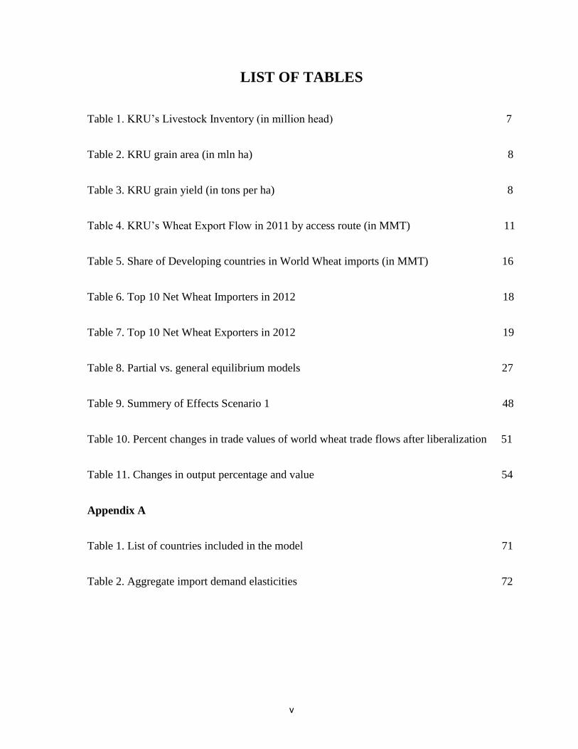
LIST OF TABLES

Table 1. KRU’s Livestock Inventory (in million head) 7

Table 2. KRU grain area (in mln ha) 8

Table 3. KRU grain yield (in tons per ha) 8

Table 4. KRU’s Wheat Export Flow in 2011 by access route (in MMT) 11

Table 5. Share of Developing countries in World Wheat imports (in MMT) 16

Table 6. Top 10 Net Wheat Importers in 2012 18

Table 7. Top 10 Net Wheat Exporters in 2012 19

Table 8. Partial vs. general equilibrium models 27

Table 9. Summery of Effects Scenario 1 48

Table 10. Percent changes in trade values of world wheat trade flows after liberalization 51

Table 11. Changes in output percentage and value 54

Appendix A

Table 1. List of countries included in the model 71

Table 2. Aggregate import demand elasticities 72

vi

Appendix B

Table 1. Summery of Effects 73

Table 2. Sensitivity analysis. Higher values of supply elasticities (increase by 0.5) 75

Table 3. Sensitivity analysis. Lower values of substitution elasticities (equal to 2) 76

vii

LIST OF FIGURES

Figure 1. Map of Black Sea wheat exporters 4

Figure 2. KRU’s transition from importer to exporter 5

Figure 3. USSR Meat Production (in Tonnes) 6

Figure 4. Market Share of major wheat exporters 9

Figure 5. World Wheat imports (in MMT) 15

Figure 6. World population towards 2050 17

Appendix A

Figure 1. Map of KRU’s exit routes to the world markets 70

Appendix C

Figure 1. Change in Russia’s Wheat export flows after liberalization 77

Figure 2. Change in Ukraine’s Wheat export flows after liberalization 78

Figure 3. Change in Kazakhstan’s Wheat export flows after liberalization 79

1

Chapter 1: Introduction

1.1 Introduction

Wheat is one of the first cereals to be domesticated in the world. It is and will likely continue

be an important part of the global food basket. World population is expected to increase by 32

percent reaching 9 nine billion by 2050 (US Census Bureau n.d.). In 2010 the world utilized 660

million metric tons (MMT) of wheat and traded 125 MMT. Ceteris paribus, in 2050 the world’s 9

billion people will consume over 880 MMT of wheat (Weigand 2011). International trade will

have a crucial role in fulfilling this increase in demand. Developing countries will account for the

majority of the predicted population growth. Population growth is the strongest in tropical and

subtropical regions where little wheat is grown.

The Food and Agriculture Organization of the United Nations (FAO 2003) projects that

developing countries will experience a significant growth in consumption. Based on forecasts of

population, wheat production and consumption, North Africa, the Middle East, Sub-Saharan

Africa, Indonesia, the Philippines, Brazil, Mexico, and India will remain the largest importing

areas. Domestic production in these countries is projected to increase by 23 percent whereas total

consumption is expected to increase by 49 percent (Weigand 2011). According to the FAO

(2003), the domestic production of developing countries will only cover approximately 86

percent of their own total need, making them increasingly dependent on imports. The task of

supplying wheat to the rest of the world will be spread among the world’s top wheat exporters;

United States, Canada, Australia, the Black Sea region (Russia, Ukraine and Kazakhstan), the

European Union and Argentina. These exporters will experience minimal or even negative

population growth towards 2050 (Weigand 2011).

2

Currently, wheat trade accounts for one third of world grain trade. Weigand (2011) concluded

that even with little import demand from China, world wheat trade is likely to double by 2050

reaching a minimum of 240 MMT.

The Black Sea region accounts for approximately one quarter of the world’s wheat exports

and is considered one of the key wheat exporting areas. The first decade of the 21st century has

been characterized by an increasing role of the Black Sea region in the global trade in wheat.

Although highly variable, the Black Sea region’s average share of world wheat exports rose from

three percent in 1992 to 12% in 2010. In comparison, over the same period the average share of

world wheat exports declined by ten percent and six percent for United States and Canada

respectively (USDA n.d.).

1.2 Problem Statement

The Black Sea Region’s accession to the WTO creates favourable conditions for its wheat

export potential. Ukraine became a member of the WTO only in 2008. Russia was accepted to

the WTO in 2012. China’s record of 12 years of accession negotiations was exceeded by

Russia’s experience. It took almost 19 years of negotiations for Russia to become a member of

the WTO. Kazakhstan is expected to follow Russia and seal a deal with the WTO members in the

near future. Kazakhstan’s negotiations have been ongoing for 16 years. The WTO accession

Working Party for Kazakhstan was established in 1996.

As a result of WTO accession, all three countries will be entitled to “most favoured nation”

(MFN tariffs), and, hence, gain improved access to potential markets previously largely

inaccessible due to very high tariffs and/or other trade barriers that can be applied on imports

from non members. For example, in 2010 China’s import duties for wheat for non-members of

the WTO were equal to 180 percent, whereas MFN tariffs were equal to 65 percent. The potential

3

decrease in tariffs is substantial. The Black Sea region’s increased market accessibility as a result

of successful accession to the WTO has the potential to bring about a major re-alignment of

world wheat trade flows, prices and changes in welfare among major wheat trading countries.

1.3 Objective of the Study

In the light of the increasing importance of world wheat trade, examining the growing role of

the Black Sea region on the international stage accompanied by trade policy changes is not only

important but also timely. Therefore, the objective of this thesis is to simulate the changes arising

in world wheat trade due to the KRU’s accession to the WTO and to estimate the changes in

trade flows, prices, tariff revenues, exporter surplus and importer surplus.

1.4 Organization of the Study

The thesis is organized as follows: Chapter 2 presents background information on the wheat

industry in KRU. Chapter 3 provides an overview of the international wheat trade. Chapter 4

touches upon the accession process to the WTO in general and the accession histories of the

KRU countries. Chapter 5 formally develops a Global Simulation Model (GSIM) for the world

wheat industry. Quantitative results are reported in Chapter 6. Chapter 7 provides the important

findings and implications. Chapter 8 concludes the thesis.

4

Chapter 2: The Wheat Industry in KRU

2.1 The Wheat Industry in KRU

The three major wheat-producing countries of the former Soviet Union − Russia, Ukraine and

Kazakhstan are becoming increasingly prominent in the global wheat trade. After the demise of

the Soviet economic system, KRU has evolved from being net wheat importing region in the

1980’s into a major wheat-exporting area and by 2005 it supplied almost a quarter of world

wheat exports. The following section will describe KRU’s transition from 1980s to the present

day and identify the possible reasons behind KRU’s emergence as an important wheat producing

and exporting region.

In wheat trade statistics, Russia, Ukraine and Kazakhstan are often referred to as Black Sea

region exporters, RUK or KRU and reported in aggregate. The following is the map of Black Sea

wheat exporters:

Figure 1. Map of Black Sea wheat exporters

Source: Dumans and Nivet, 2003

5

The Black Sea is the main avenue for accessing world markets for all three countries. Figure 1

shows the seaports on the Black Sea used by grain exporters and important export destinations.

Russia and Ukraine have the advantage of having several seaports. Ilychevtsk, Odessa and

Mykolaev are Ukraine’s main seaports located in the Black Sea. Russia possesses both Baltic Sea

and Black Sea exits to the world grain markets; Rostov and Novorossisk in the Black Sea,

Kaliningrad and St. Petersbourg in Baltic Sea (see Figure 1). Kazakhstan, on the other hand, has

no direct access to the Black Sea due to the landlocked nature of its territory. A more detailed

discussion on transportation and logistics will be presented in the transition problems and

constraints section below.

The following is a brief timetable showing KRU’s transition from being a major wheat

importer as part of the USSR to becoming a major exporter in the 2000s (see Figure 2)

Figure 2. KRU’s transition from importer to exporter

The last decade of the USSR’s existence can be characterized by an intensification of the

agricultural production. The major focus was given to cereal production, particularly winter

wheat, and meat production. The Soviet government intended to increase consumers’ standard of

living through increased consumption of meat and dairy products (Liefert et al. 2013).

1970's-1980's Soviet

Union as an importer

1991 End of Soviet Union.

KRU's minor exports

2000-2012 KRU

becomes a major exporter

2020-2030 KRU exports

expected to grow

6

From: (FAOSTAT n.d.)

Figure 3 illustrates the increase in the USSR’s meat production, particularly from 1970 up until

1990. Domestic grain production could not satisfy the need to feed the ever increasing numbers

of livestocks; therefore the Soviet Union had to import grain (Liefert et al. 2013)

The transition from central planning to a free market-based economy has been difficult

for all three economies. As in the case with the broader economy, agricultural production

plummeted with the collapse of central planning. The 1990s were characterized by a contraction

in agricultural production, particularly livestock production. KRU’s animal numbers shrank by

more than half. Liefert et al. (2013) argue that the decline of livestock production during the

economic transition has been the major reason for KRU countries moving from being grain

importers to grain exporters. The Table 1 illustrates the decrease in livestock inventory in KRU.

There was a dramatic decrease in livestock inventory over the period from 1990 to 2011. For

example, the number of cattle in Ukraine declined from 25.2 million head in 1990 to 4.5

7

million head in 2011. The number of sheep and goats shrank from 9 million head in 1990 to just

1.7 million head in 2011.

The number of pigs declined from 19.9 million head in 1990 to 8 million head in 2011. Similar

trends in livestock inventory can be observed in Kazakhstan and Russia.

The second reason behind KRU’s increased exports is the rise of grain production in the

2000s after a decline in early years of transition. The increase in grain production is due to

increased yields rather than an expansion of the land being cropped. The KRU utilized less area

for grain production in 2011 than in the 1980’s. This could be partially due to the fact that during

the Virgin Lands1 campaign, the massive increase in cropland fostered by the policy expanded

into areas not really suitable for grain production2.

1 Virgin Lands campaign is the Soviet government’s (namely Nikita Khrushev’s) plan to boost the agricultural

production. The campaign was implemented during 1950’s and early 1960’s. 2 USSR’s eastern part of the grain belt (Kazakhstan, West Siberia) was particularly unsuitable for grain production

due to climatic conditions (Felix,1981).

Large horned

livestock

Sheep and

goatsPigs

Large horned

livestock

Sheep and

goatsPigs

Large horned

livestock

Sheep and

goatsPigs

1990 n.d n.d n.d 25.2 9.0 19.9 9.8 35.7 3.2

1991 n.d n.d n.d 24.6 8.4 19.4 9.6 34.6 3.0

1992 52.2 51.4 31.5 23.7 7.8 17.8 9.6 34.4 2.6

1995 39.7 28 22.6 19.6 5.6 13.9 6.9 19.6 1.6

2000 27.5 15 15.8 10.6 1.9 10.1 4.1 10.0 1.1

2005 21.6 18.6 13.8 6.9 1.8 6.5 5.5 14.3 1.3

2007 21.5 21.5 16.3 6.2 1.6 8.1 5.8 16.1 1.4

2008 21 21.8 16.2 5.5 1.7 7.0 6.0 16.8 1.32009 20.7 22 17.2 5.1 1.7 6.5 6.1 17.4 1.3

2010 20 21.8 17.2 4.8 1.8 7.6 6.2 18.0 1.3

2011 20.1 22.9 17.3 4.5 1.7 8.0 5.7 18.1 1.2

Note: Russian statistics does not report some years. Therefore those years were removed from the table.

From: Statistics Agency of Kazakhstan n.d. RF Federal State Statistics Service n.d , State statistics services of Ukraine n.d

Russia Ukraine Kazakhstan

Table 1. KRU's Livestock Inventory (in million head)

8

The Table 2 reports the changes in the area of grain production in the KRU over the

period between 1987 and 2010.

Russia Ukraine Kazakhstan KRU in total

1987-91 59.4 13.3 23.3 96

1992-95 54.7 12.2 20.8 87.4

1996-2000 47.4 11.9 13.3 72.6

2000-2005 42.7 13 13.9 69.6

2006-2010 42.7 13.9 15.9 72.5

Table 2. KRU grain area (in mln ha)

Note: Figures are average annual values during the period.

From: FAS Production, Supply and Distribution Online (USDA 2013)

The area used for grain production fell during the early transition period in all three KRU

countries. In 2010, the KRU countries were still using less land for grain production than they

were in 1987. According to Prikhodko (2009), approximately 13 million ha of land can be

returned into grain production in the KRU countries at no major environmental costs. However,

returning idle lands back to production incurs additional costs for clearing and preparing the land

for cultivation.

The decrease in wheat yields in the KRU during the 1990s, followed by a small increase

in the 2000s can be seen in Table 3.

Russia Ukraine Kazakhstan

1987-91 1.61 3.27 0.89

1992-95 1.53 2.91 0.9

1996-2000 1.33 2.18 0.84

2000-2005 1.79 2.62 1.04

2006-2010 1.92 2.81 1.06

Note: Figures are average annual values during the period.

From: FAS Production, Supply and Distribution Online

(USDA 2013)

Table 3. KRU grain yeild (in tons per ha)

9

Yields in Russia and Kazakhstan have increase only marginally from 1987 to 2010, while the

average grain yield in Ukraine decreased. Liefert et al.’s (2013) analysis indicates that the small

increase in yields can be attributed to a rise in input productivity and favorable weather condition

during the 2000s. However, yields in the KRU countries are still far below those in Canada, the

USA or the EU3.

In the 2000s, KRU countries become major exporters and were responsible for almost a

quarter of the world wheat exports by 2008. Figure 4 clearly demonstrates the growing

importance of the KRU countries in international trade.

From: USDA, Foreign Agricultural Services, Production, Supply and Distribution (PS&D)

Database (USDA n.d.)

KRU’s export share increased from only 2 percent in 1991 to 23 percent in 2008. Future

projections are positive for KRU’s exports. By 2021, KRU is expected to account for 30 percent

3 In comparison, the average yield for the 2006-2010 periods is equal to 2.9, 5.25 and 2.67 tones per hectare in US,

EU and Canada respectively (FAOSTATa n.d.)

10

of world wheat exports (USDAa n.d.). Ultimately however that will depend on the KRU

countries’ ability to overcome some major transition problems and constraints.

2.2 Transition Problems and Constraints

Russia, Ukraine and Kazakhstan hold significant potential to expand their wheat exports.

However, transportation and logistics problems as well as outdated agricultural equipment and

practices continue to be major issues for KRU countries. Hence, it is worth keeping in mind that

the major findings of the present research are subject to careful interpretation. For example,

changes in future projected wheat trade between Kazakhstan and EU might not be achieved due

to Kazakhstan’s transportation constraints. All of the KRU countries are still countries in

transition and, hence, do not exhibit the same levels of efficiency as can be achieved in modern

market economies. Further, their ability to respond to incentives may be inhibited.

The KRU countries possess several exit routes to world wheat markets. They are Black

Sea ports, Baltic Sea ports, Far Eastern ports, shallow water ports4 and, the Azov Sea and rail

routes. A map of the KRU’s exit routes is provided in the Appendix A. All three countries are

interested in increasing their grain handling capacities.

There is a lack of official information on the exact capacities of ports and grain terminals.

Therefore the information presented in this section is sourced primarily from various reports and

newsletters. Numerical data on ports and terminal capacities are from estimates provided by

market analysts. According to Vassilieva and Flake (2011), Russia’s overall port capacity is

estimated at 25 million metric tones of wheat a year. Ukraine’s export capacity (Black Sea and

Azov Sea) is estimated at more than 26 million metric tones a year (Prikhodko 2009).

Information on Kazakhstan’s exact export capacity is non-existent.

4 Shallow water ports are ports along rivers.

11

The Black Sea ports are for the most part utilized by Ukraine and Russia. The ports of

Novorosiisk, Tuapse and Taman are the larger ones utilized by Russia. Ukraine is in the most

advantageous position in terms of reaching the Black Sea. It has Ilychevtsk, Odessa and

Mykolaev and other smaller ports.

Ukraine and Russia also possess shallow water ports such as those at Rostov-on-Don,

Azov, Temruk, Kavkaz, Taganrog, and terminals on the Volga-Don (Vassilieva and Flake 2011).

Most of these terminals are low capacity terminals that operate seasonally due to the rivers icing

up.

Kazakh wheat has to travel at least 3500 kilometers to reach the Black Sea and faces

competition from the other two countries. Therefore, the use of Black Sea ports’ by Kazakhstan

is limited. Kazakhstan has an access to world markets in the Caspian Sea and transports grain to

the Black Sea and Baltic Sea by rail. Rail is also heavily used for exports to the neighboring

central Asian countries. Table 4 shows KRU’s actual wheat export quantities by the mode of

transportation/access route.

As can bee seen from the Table 4, Black Sea deep-water ports are primarily used by Russia and

Ukraine, Baltic Sea ports are utilized by Russia and Kazakhstan. Wheat exports from Kazakhstan

to the neighboring countries, including China, are shipped by rail.

Black Sea

deep water

ports

Black Sea

shallow

water ports

Baltic portsTrains to

export

Total

Export

Russia 12 6 1 19

Ukraine 7.5 1 0 8.5

Kazakhstan 2 1 2 2.5 7.5

Table 4. KRU's Wheat Export Flow in 2011 by access route (in MMT)

Adapted from Boersch (2013).

12

According to Prikhodko (2009), Russia will increase its port capacity to handle 28 MMT

of grain a year by 2015. Asian pacific markets are becoming more attractive to Russian wheat

producers. Therefore, the Russian government is interested in developing grain terminals and

increasing port capacity in Vladivostok on the Pacific (Baltinfo n.d.). The major concern is the

cost of transportation from Siberian and Ural regions to Vladivostok.

Inadequate grain handling capacities, logistics problems and aging rail infrastructure

remain the main constraints faced by wheat producers in Russia. Seventy seven percent of the

grain handling railway wagon fleet is expected to be written-off by 2015 (Baltinfo n.d.).

Ukraine is the most fortunate of the KRU countries in terms of transportation costs. This

is due to the short distances to the Black Sea. Ukraine’s transportation constraints are largely

related to low rural railway loading capacities and poor administration of the rail system

(Boersch 2013).

Kazakhstan is also making efforts to increase its grain-handling infrastructure.

Government officials expressed willingness to increase access to Middle Eastern markets by

developing a rail line south from Kazakhstan through Turkmenistan to Iran (Prikhodko 2009).

Kazakhstan is also planning to build terminals in Belorussia for grain shipment from the Baltic

Sea. The recently developed Dostik-Alashankou rail route provides access for Kazakh grain to

China and is now fully operational. Overall, the main obstacles faced by Kazakh wheat exports to

the world markets are high transportation costs, restricted access to terminals and elevators in

Black Sea ports and the risks associated with domestic policies5.

It is difficult to talk about the farm level constraints across KRU countries in generalized

terms. Nevertheless, it is evident that agro-holdings, also referred to as New Agricultural

5 Example: an export ban.

13

Operators, play a significant role in grain production in all KRU countries. There presence,

however, varies in the three countries (Fellmann and Nekhay 2012). In Kazakhstan, twenty big

companies account for approximately 80 percent of the grain output. Two hundred companies

account for about 25 percent of the grain output in Russia. The importance of agro-holdings in

the Ukraine is less prominent but they rapidly increased their operation in the second half of the

2000s. The average size of the agro-holding is 100 000 ha (Prikhodko 2009).

Agro-holdings are vertically integrated entities that include agricultural production and

processing facilities as well as grain elevators situated on the transport systems. They hold

various advantages compared to smaller farms in terms of attracting investments, input purchases

etc. The expansion of such integrated enterprises has been achieved through the acquisition of

indebted former collective farms and elevators. Bank loans for large acquisitions are usually

secured by the major downstream enterprises or holding companies (Wandel 2008). Apart from

their own retained earnings, agro-holdings have access to bank loans for financing new

technologies and western machinery. An agro-holding is controlled by a headquarters that is

responsible for all financial, marketing and remote management activities of the enterprise. They

enjoy economies of scale in terms of bulk input purchases and expert staff. Vertical integration

allows for a better control over production methods, the quality of inputs and supply of outputs

including exports of wheat. Agro-holdings maintain close relations with local authorities as well

as with policy makers. These relationships allow them to garner state support when needed.

Overcoming the major constraining factors faced by KRU is a matter of time and

resources. Therefore, any significant changes in trade flows projected by the model are most

likely achievable in the long run only.

14

2.3 Summary

The KRU countries have become increasingly important in the world wheat trade. From

being grain importers as part of the USSR, these three countries evolved into major wheat

exporters. The transition from centrally planned command economies to the ones governed by

market mechanisms has been difficult and is still continuing. Agriculture went through a major

decline after the collapse of the Soviet Union. A drastic decline in livestock numbers, a marginal

increase in yields and favorable weather conditions are considered to be the major factors that

contributed to the increase in the KRU countries’ wheat exports. In 2008, the KRU region

accounted for almost a quarter of the world wheat export market share and is expected by some

to play an increasingly important role on the international stage in the future. However, transition

problems and constraints remain. Significant investments in infrastructure are required to remove

many of the constraints faced by KRU countries. Poor infrastructure, antiquated logistics and

bottlenecks may yet hinder the KRU’s potential capacity to increase grain exports.

15

Chapter 3: International Wheat Trade

Wheat trade is and will likely be an increasingly important component of world trade in

agrifood products and a contributor to global food security. Wheat accounts for one third of the

world’s trade in cereals. In 2010, the world utilized 666 MMT and traded 126 MMT of wheat

(FAO n.d.). Figure 5 shows the increasing importance of world wheat trade currently and in the

future.

From (OECD-FAO 2012)

Most of the demand for wheat imports arises from the developing countries. In 2012, developing

countries accounted for eighty percent of global wheat imports and are expected to account for

approximately eighty percent of the demand for wheat imports in the future (see Table 5)

(OECD-FAO 2012).

16

YearWorld Total

imports

Developing

countries

Developing

countries in

% from

total world

imports

2012 137 110 80

2013 137 111 81

2014 137 111 81

2015 139 113 81

2016 140 115 82

2017 144 118 82

2018 145 120 83

2019 148 123 83

2020 150 125 83

2021 152 127 83

Table 5. Share of Developing countries in World

Wheat imports (in MMT)

From: OECD-FAO (2012)

Increase in wheat consumption is often associated with the increase in population because these

two mirror each other. According to US Census Bureau, the world population will reach 9 billion

people by 2050 (US Census Bureau n.d.). Figure 6 shows the expected increase in world

population. Developing countries will account for the majority of the predicted population

growth. Population growth is the strongest in tropical and subtropical regions where little wheat

is grown.

As reported above, in 2010 the world utilized 666 MMT of wheat and traded 126 MMT

of wheat. Ceteris paribus, in 2050 the world’s 9 billion people will consume over 880 MMT of

wheat (Weigand 2011). Based on population growth, wheat production and consumption

projections, Weigand (2011) concluded that even with little import demand from China, world

wheat trade is likely to double by 2050 reaching a minimum of 240 MMT. International trade

will have a crucial role in fulfilling this increase in demand.

17

Various agricultural outlooks and market analysis reports identify several geographical

regions where wheat is an important factor in future wheat production and/or consumption: North

America, South America, Central America, EU, rest of the Europe, Middle East, North Africa,

Sub Saharan Africa, East Asia, South Asia, South East Asia, the Former Soviet Union and Others.

Market analysis discussion by FAO, UNDP, etc. usually provide statistics and forecast for the

aggregated regions listed above.

From: UN Department of Economic and Social Affairs, Population Division (2011)

The FAO (2003) projects that developing countries will experience a significant growth in

consumption. Based on forecasts of population, wheat production and consumption, North Africa,

the Middle East, Sub-Saharan Africa, Indonesia, the Philippines, Brazil, Mexico, and India will

remain the largest importing areas. Domestic production of these countries is projected to

increase by 23 percent whereas total consumption is expected to increase by 49 percent

(Weigand 2011). According to the FAO, domestic cereal production of developing countries will

only cover approximately 86 percent of their own total need, making them increasingly

18

dependent on imports (FAO 2003). The task of supplying wheat to the rest of the world will be

spread among the world’s top wheat exporters; the United States, Canada, Australia, the Black

Sea region, EU and Argentina. These exporters will experience minimal or even negative

population growth towards 2050.

Table 6 provides the list of the top ten wheat importers in the world in 2012.

Rank Country Quantity (in Million tons)

1 Egypt 9.3

2 Indonesia 6.3

3 Brazil 6.0

4 Japan 5.6

5 Algeria 5.2

6 Morocco 4.4

7 South Korea 4.3

8 Iraq 3.7

9 Iran 3.6

10 Mexico 3.4

Total Imports 139.4

Table 6. Top 10 Net Wheat Importers in 2012

From: USDA, Foreign Agricultural Services, Production,

Supply and Distribution (PS&D) Database (USDA n.d.)

As can be seen from the Table 6, the top wheat importers are all countries of North Africa,

Middle East, Asia and South America. Table 7 provides a list of top ten wheat exporters. Russia,

Ukraine and Kazakhstan are all included in the top ten list of exporters. They are reported

separately in Table 7, however combined KRU exports are slightly less than US exports and

exceed those of Canada.

19

Rank Country Quantity (in Million tons)

1 United States 25.0

2 Canada 18.1

3 Australia 16.4

4 European Union 12.0

5 Russia 9.0

6 Kazakhstan 7.0

7 India 6.5

8 Ukraine 6.1

9 Argentina 5.0

10 Uruguay 1.0

Total Exports 132.0

From: USDA, Foreign Agricultural Services, Production,

Supply and Distribution (PS&D) Database (USDA n.d.)

Table 7. Top 10 Net Wheat Exporters in 2012

In short, the importance of world trade in wheat is expected to grow. Developing

countries of North Africa, the Sub-Saharan region, the Middle East, South America and Asia will

experience the greatest increase in population and are expected to generate most of the increase

in demand for wheat in the future. On the other hand, traditional wheat exporting countries will

experience no dramatic increase in population or changes in consumption and therefore have the

opportunity to fill in the gap in the increasing demand for wheat.

Trade barriers however, constrain trade in wheat and alter its distribution among countries.

A major change in trade constraints, such as those arising from accession to the WTO, can have a

major impact on the international trade in wheat. The affect of WTO accession on trade barriers

is provided in Chapter 4.

20

Chapter 4: The WTO Accession Process

4.1 The WTO Accession process

One of the oldest forms of international relations is international trade. Accelerating the

international division of labour, foreign trade was and remains a basis of the international

economic relations that connects all countries to the global economy. Foreign trade can play a

vital role in a country’s economic growth and development. As with any international relations,

there is a need for rules of conduct. This is particularly true in the case of international trade.

Firms that wish to make investments in international trading activities need to know that their

investments are not at risk from governments acting in ways that make what were initially

profitable investments, unprofitable. For example, governments can put a profitable investment

at risk by putting in place trade barriers. The World Trade Organization is the most important

multilateral trade institution that administers an agreed set of rules for international trade rules

that have been agreed, to date, by 159 countries. Formed in 1995, as a successor to the General

Agreement on Tariffs and Trade, the WTO administers the agreed rules of international trade.

The WTO rules govern approximately 97 percent of global trade.

Making trade flow smoothly and in predictable ways is at the core of the existence of the

WTO trading system. The WTO lists numerous benefits 6 arising from its existence that

collectively promote international development, cooperation and confidence. Confidence in

being treated equally and fairly is important for countries, and their firms that wish to invest in

international trade activities. Being a member of the system of agreed rules means that a firm is

6 The ten benefits of joining the WTO: 1. The system helps promote peace. 2. Disputes are handled constructively. 3.

Rules make life easier for all. 4. Freer trade cuts the costs of living. 5. It provides more choice of products and

qualities. 6. Trade raises incomes. 7. Trade stimulates economic growth. 8. The basic principles make life more

efficient. 9. Governments are shielded from lobbying. 10. The system encourages good government (WTO n.d.)

21

better shielded from unfair treatment, sudden protectionist measures or other political matters.

Membership means being not discriminated against and being entitled to receive the same trading

conditions as every other member of the WTO. Of course, trade disputes will remain, however

the WTO trading system with a set of rules and conditions reached by consensus allows the

handling trade disputes in a transparent and structured manner. The equality provided by the

WTO membership manifests itself through the import tariffs that firms face in foreign markets.

There is a considerable difference between tariffs applied to members and non-members of the

WTO. Countries are not entitled to MFN tariffs unless they are members of the WTO.

Before enjoying the security provided by WTO membership, each country wishing to join

the WTO has to go through a five-stage accession process. First, after gaining observer status, the

country has to submit a memorandum outlining how its trade and economic policies align, or not,

with the WTO’s agreed rules. The memorandum is examined by a Working Party that includes

all interested member countries. After a Working Party has made sufficient progress on ensuring

the applicant country’s policies align with the rules, countries start bilateral negotiations.

Although each interested country negotiates on tariff reductions and other trade inhibiting

policies that determine export opportunities for its exporting firms, commitments made in

bilateral negotiation will apply equally to all other members following the WTO principle of

non-discrimination. The number of bilateral negotiations depends on the number of countries that

comprise the Working Party. The third step starts when the applicant’s trade regime is re-

examined for compliance with the rules and bilateral talks are complete. The final accession

terms are reflected in a formal protocol of accession and tariff schedules. The fifth and final step

is the submission of a final package that consists of the protocol and schedules. The final package

is presented to the WTO General Council or a Ministerial Conference. The observer is then free

22

to join the organization if two-thirds of the WTO members vote in the affirmative (WTO

Information and External Relations Devision 2011)

4.2 The History of Accession for KRU countries

Accession to the WTO promotes the further integration of a country into modern

economic trade relations. The duration of the process of accession to the WTO differs from one

case to another depending on the number of bilateral negotiation that have to be completed to

achieve consensus. Political matters can also slow the accession process down. For comparison,

it took nineteen years of negotiations for Russia to become a member of the WTO but, for

example less than three years for Kyrgyzstan.

After the demise of the Soviet Union and the achievement of independent country status,

Russia, Ukraine and Kazakhstan applied for membership in the World Trade Organization.

Russia was first to express its willingness to join the WTO (GATT7 at the time). In June 1993,

Russia submitted the official application to the Secretariat of the GATT. The Working Party

chaired by Mr. W. Rossier8 (Switzerland) was established the same year and consisted of 58

members. Subsequently, the Working Party was chaired by two other ambassadors − Kare Bryn

(Norway) from 2000 to 2003 and Stefán Jóhannesson (Iceland) from 2003 to 2011. A

memorandum on Russia’s Foreign Trade regime was circulated by the Secretariat in 1994. The

process proceeded with questions and feedback to Russian authorities. The Working Party

meetings commenced in 1995. There were, in total, 31 formal Working Party meetings as well as

numerous informal ones. The most difficult bilateral negotiations were those with the EU, China,

7 GATT-General Agreement on Tariffs and Trade was replaced by WTO on January 1, 1995 under the Marrakesh

Agreement 8 Different country representatives at the United Nations and other international organizations in Geneva usually

chair the WTO working parties.

23

the US and during most recent years Georgia9 (Babkin et al. 2012). After 2000, the negotiations

covered all aspects of Russia’s accession to the WTO including it’s commitments concerning the

tariff schedule, market access to goods and services and agriculture. Finally, nineteen years of

difficult negotiations yielded results. Russia’s accession package, the biggest accession package

in the history of the WTO, was approved by the Eighth Ministerial Conference in 2011. On

August 22, 2012 Russia notified the WTO Secretariat of the ratification of the package and

officially became a member of the WTO.

Among KRU countries, Ukraine was the first to accede the WTO. Ukraine submitted its

application to the WTO after Russia, in November 1993. The Working party was established the

same year in December. The memorandum on Ukraine’s trade regime was circulated in 1994.

Throughout the accession process, Ukraine’s Working party was chaired by three ambassadors;

Mr. A. Stoler (US), Mr. S. Marchi (Canada) and Mr. M. Matus (Chile). The process of Ukraine’s

accession can essentially be divided in to three periods. The first period, 1993-1997, was

dedicated to the analysis and monitoring of the economy to determine if it reflected GATT/WTO

norms and regulations. The second period, 1998-2003, entailed the process of enforcing laws

deemed a priority for accession in order to adjust regulations in accordance with the WTO norms.

The final, stage, 2003-2008, can be described as a process of identifying Ukraine’s commitments

regarding its membership to the WTO. The 2005-2007 period produces a breakthrough in the

negotiation process. During that period Ukraine was able to reach agreement with 52 member

states of the WTO and ratify 55 laws in accordance with the WTO norms (Pugachev 2012). In

2008, after 15 years of negotiation, Ukraine was officially welcomed into the WTO.

The negotiation process for Kazakhstan’s accession to the World Trade Organization

started on the 29th of January in 1996, with the submission of the official application to

9 An armed conflict between Georgia and Russia took place in August 2008.

24

Secretariat of the WTO. In February of the same year, Kazakhstan was assigned status as an

“observer” country to the WTO. On April 16, in 1996, the General Council of the WTO

established a Working Party to examine the application and provide recommendations, including

comments on a draft of the Protocol of Admission. Any interested member country could join the

Working Party. Members of the Working Party were then encouraged to submit questions on

Kazakhstan’s Memorandum on its Foreign Trade regime that was circulated by the Secretariat,

on 11 November, 1996. The feedback and questions were then transmitted to the Kazakhstan's

authorities for further examination and comment. The Memorandum reflected on Kazakhstan’s

economy, economic policies and foreign trade regimes at that time. Government officials

acknowledged that Kazakhstan’s key trade legislation met the most important WTO principles

and committed Kazakhstan to bringing them in to full compliance with the WTO’s agreed rules.

All the ministries of the Kazakhstan Government were urged to ensure full compliance of their

legislation with the WTO standards (WTO 1996). To date, Kazakhstan’s Working Party consists

of 43 members and is chaired by H.E. Mr. Hannu Himanen. The Working Party members include

the EU and its members as one. Each bilateral negotiation has to finish with a bilateral agreement.

Members of the Working Party consist of all the main trading partners of Kazakhstan that belong

to the WTO which have expressed a desire to discuss conditions for, and obligations of, the

country’s accession to WTO. Kazakh government officials have been releasing statements which

anticipated accession each year since 2010. Hence, it is difficult to determine whether

Kazakhstan will finally accede to the WTO by the end of 2013, as is planed.

4.3 Summary

KRU countries have gone through a long accessing journey. Russia and Ukraine have

successfully joined the WTO, while Kazakhstan is expected to join them shortly. To date, the

WTO governs the trade between 159 countries. Becoming a member of the WTO trading system

25

is an important step towards integration into the world economy for every country. Most of all,

membership in the WTO provides confidence. In other words, membership provides equal access

to markets and a common trade dispute resolution mechanism. Before enjoying the confidence

offered by the WTO, each country has to go through a five-stage accession process. First, the

potential accessing country submits its Memorandum on foreign trade. The second stage involves

revision of the memorandum by the Working party. The third stage begins with the re-

examination of the trade regime according to the WTO rules and bilateral negotiations.

Accession terms are then reflected in a formal protocol and presented to the WTO General

Council or a Ministerial Conference as a final package. Once the final package is voted in

affirmative by the two-thirds of the WTO members, the observer country if welcomed to join the

WTO.

Given that the KRU countries accession to the WTO will result in those countries being

eligible to have MFN tariff applied on their wheat, important changes in the world trade in wheat

can be anticipated. In Chapter 5, those expected changes are formally modeled.

26

Chapter 5: Modeling Global Wheat Trade

5.1 Literature review

Considerable effort has been devoted to developing models that can be applied to trade

policies for agricultural products. Building an applied trade model is a costly, rigorous process

that requires time and effort to be spent on assembling a database, the formulation of the

theoretical underpinnings, obtaining estimates of parameters and shocking the model in

simulations (Tongeren et al. 2001). None of the existing modeling approach is flawless. In each

particular case one model is more applicable than the other. A detailed and comprehensive

review and assessment of the existing global models applied to agriculture and trade policies is

provided by Tonegeren et al. (2001). They discuss a number of partial equilibrium and general

equilibrium models developed in the 1990s. Their review provides a comparative assessment of

alternative modeling approaches by highlighting common features, differences and areas of

applicability10. Of course, no model is appropriate for all purposes. Researchers have to use their

own judgment and choose a model that is capable of providing answers to the question of interest

given the information available and constraints on research resources.

In general terms, modeling approaches differ based on scope, specifications, assumptions,

etc. Trade models are often multiregional. Multiregional trade models can differ with respect to

the regional coverage. Some models focus on a certain set of trading partners, whereas others

attempt to account for worldwide trade. A set of countries are often aggregated as one block such

as the previous 15 members of the European Union (EU-15)11, the former Soviet Union (FSU) or

the Rest of the World ROW (ROW). Models differ in terms of being dynamic or static, partial or

10 For a detailed discussion and list of agricultural policy models see F. von Tongeren et al. (2001) 11 EU-15 countries are: Austria, Belgium, Denmark, Finland, France, German, Greece, Ireland, Italy, Luxembourg,

Netherlands, Portugal, Spain, Sweden and United Kingdom.

27

economy-wide models. Dynamic models allow for time and adjustment paths. Static models

observe differences between equilibriums resulting from the shocks in variables (for example,

policy changes or crop failures).

A choice between a partial-equilibrium (PE) and a general-equilibrium (GE) modeling

approaches is one of the key decisions faced by the analyst. This choice involves a trade-off. This

trade off is best demonstrated in the following Table 8. (see Table 8).

PE GE

Capturing economy wide linkages x

Consistency with the budget constraints x

Capturing disaggregated effects x

Capturing complicated policy mechanisms x

Use of timely data x

Capturing short and med. term effects x

Capturing long term effects x

Source: Bacchetta et al, 2012

Table 8. Partial vs. general equilibrium models

General-equilibrium models are able to capture economy-wide linkages and long term effects of

the shocks. Partial equilibrium (PE) models, on the other hand, can be as disaggregated as one

wishes. Partial equilibrium models are generally easy to use and straightforward to interpret as a

relatively limited number of equations are used to calculate changes in demand and supply. As

only one sector is modeled, PE models typically require less data than GE models: usually trade

flows, trade policy data and elasticities (Bacchetta et al. 2012). PE models’ simplicity and ease,

however, is partially offset by a number of limitations. One of the major limitations is that PE

models do not include constraints on factors of production. Second, PE model results are

sensitive to the chosen values of elasticities. Effects on other markets are also lost.

Despite these limitations, PE models are widely applied to research on an industry level.

Partial equilibrium models of trade in agriculture are often focused on primary commodities.

28

Partial equilibrium models treat agricultural trade as being isolated from the rest of the economy.

Economy-wide GE models, on the other hand, account for inter-industry relations, thus allowing

the implications of international trade on the economy as a whole to be observed. Economy-wide

models are, of course, much more data intensive than the partial equilibrium models. Parameter

estimates such as price and income elasticities, and/or substitution elasticities are also crucial for

GE modeling approach. These key parameters determine the extent of response shocks including

policy changes. They must be consistent with the available data and economic theory (Tongeren

et al. 2001). Key parameters can be determined via two different approaches, either

econometrically or by calibration. Econometric estimation of parameters is resource intensive

and should be performed by simultaneous equation estimation methods that take into account the

overall model structure (Tongeren et. al. 2001). Calibration, also known as the “synthetic

approach”, is a more popular because it is much less resource intensive. Using estimates of

elasticities from existing sources, the calibration approach generates parameters consistent with

the pre-shock benchmark data and the theory underlying the model.

Due to their simplicity and transparency, partial equilibrium models have been widely

used in the policy assessment and economic welfare literature. Partial equilibrium models range

from simple single market representations to more complicated, multi region global models.

Recent partial equilibrium agricultural trade models include the USDA’s Statistical World Policy

Simulation (SWOPSIM) developed by Roningen et al. (1991), World Bank and UNCTAD

Software for modeling Market Analysis and Restrictions on Trade (SMART), the Agricultural

Trade Policy Simulation Model (ATPSM) developed by United Nations Conference on Trade

and Development (Vanzetti and Peters 2004, Bacchetta et al. 2012) and the Global Simulation

model (GSIM) developed by Francois and Hall (2003).

29

Economy-wide models have been developed by the Global Trade Analysis Project

(GTAP) by Hertel (1997), the US Applied General Equilibrium model developed by the

International Trade Commission (USITC 2004), MEGABARE and GTEM developed by the

Australian Bureau of Agriculture and Resource Economics (ABARE 1996). The list of modeling

approaches mentioned in this review is by no means exhaustive. This review is focused mainly

on the models utilized specifically in agricultural trade policy and welfare research.

Most of the research related to modeling world wheat markets dates back to 1970s. Early

studies accounted for the Soviet Union as a single market. In the 1990s, Russia, Kazakhstan and

Ukraine were not yet considered as important exporting countries and, therefore, were often

ignored in the model design. Further, command economy era data was not considered reliable

and these economies exhibited considerable disequilibrium in the early years of transition. The

latter meant that the data was unreliable for modeling purposes because the adjustments

processes required to reach equilibrium were not well understood. The following is a short

description of a number of models used specifically to examine the international market for

wheat.

Large and complicated models applied to trade in wheat were developed by Devadoss et

al. (1990) and Roningen et al. (1991). The Food and Agriculture Policy Research Institute

(FAPRI) model produced by Devadoss et al. (1990) incorporates a set of models that can

determine the effects of alternative farm policies and program proposals on agricultural

commodity markets as well as the agricultural sector of the US. In general, models are solved

iteratively to arrive at a simultaneous solution. A solution is obtained whenever the demand is

equal to supply in each market, and the same vector of prices and other endogenous variables is

obtained for all component models (Devadoss et al. 1990). One of the set of FAPRI models is

focused specifically on trade in wheat. It is a non-spatial, partial equilibrium model. Non-spatial

30

means it does not identify trade flows between specific countries (Devadoss et al. 1990). The

model consists of domestic supply and demand functions for major wheat trading and producing

countries and regions. Equilibrium prices, quantities and net trade are determined by equating

import and export functions of different regions and linking regional prices to world prices.

Being fairly detailed, this trade model has been used to analyse the impacts of exogenous shocks

such as technological change, yield changes, income growth, inflation, or changes in exchange

rates, etc. FAPRI is often used in United States Department of Agriculture (USDA) and

Agriculture Policy related institutions’ publications. Although primarily focused on the US, the

FAPRI model has been used to produce global agricultural commodity outlooks. One of the

major features of the FAPRI model is its ever expansion. The model is always kept updated and

is being enhanced in order to address novel policy questions. The benefits from an expanded

model, however, carry certain costs. Although a larger model is suited to a broader range of

questions, less focus can be given to any one specific part of the model (Meyers et al. 2010).

The Static World Policy Simulation (SWOPSIM) model developed by Roningen et

al.(1991) has also been used extensively in USDA research. It is a static, partial equilibrium

model that simulates the effects of changes in agricultural support on production, consumption

and trade. Most of the research utilizing the SWOPSIM model dates back to the 1980s.

According to Tongeren et al.(2001), the model is no longer in use.

Both FAPRI and SWOPSIM assume homogeneity of wheat across countries. Benirschka

and Koo (1995) have relaxed the assumption of homogeneity. They developed a dynamic multi-

commodity model that includes eleven wheat classes. The World Wheat Policy Simulation

model is a hybrid between an econometric model and a synthetic model, meaning that some of

the behavioural equations are estimated while others are based on synthetic parameters

(Benirschka and Koo, 1995). A different approach was taken to modeling the exporting and

31

importing sub models that account for acreage harvested, yield, production, domestic

consumption, and carryout stocks. The import side country sub models were estimated based on

Armington’s12 approach to demand. This approach reduces the number of parameters that have

to be estimated and allows for product differentiation.

Another method that has been used in wheat trade research is that of Spatial Equilibrium

modeling (SEM). Gomez-Plana and Devadoss (2004) provide an evaluation of trade policy

impacts in world wheat markets using SEM. They argue that the wheat markets’ price decline in

the early 2000’s can be attributed to a surge in supply combined with restrictive trade barriers.

The study provides a simulation of the elimination of all import tariffs and subsidies. The effects

of trade liberalization are reported in terms of changes in price, supply, demand, imports, exports

and welfare changes in each region/ country. A spatial equilibrium model popularized by

Takayama and Judge (1971) was adapted for the wheat market. Thirty two countries were

included in the modeling exercise. They are separated by distance and are assumed to trade

homogeneous wheat competitively. SEM employs a non-linear optimization to maximize the net

social monetary gain function, subject to a set of constraints (Gomez-Plana and Devadoss 2004).

Elasticity parameters were adopted from secondary literature. Gomez-Plana and Devadoss (2004)

arrived at the following main conclusions: wheat trade liberalization leads to an increase

(decrease) in prices in the exporting (importing) country; production and exports increase in the

exporting countries, consumption and imports increase in importing countries. As a result, there

is an overall increase in trade. Most of the countries gain as a result of more trade; hence, there is

an overall world welfare increase.

12 Armington (1969) proposed a general theory of demand that distinguishes products according to their place of

production. The Armington assumption states that products traded internationally are differentiated by the country of

origin. The source of differentiation can be different bilaterally applied tariffs between countries

32

A spatial model refers to a mathematical programming model that focuses on

transportation costs (Benirschka and Koo 1995). Accounting for transportation costs in a global

scale trade modeling exercise is problematic. Choosing proxies for transportation costs in world

wheat trade for each country is cumbersome. Obtaining reliable transport cost data is one of the

main difficulties in analysing transportation (Inmaculada and Celestino 2005). There are,

however, official sources that provide fairly detailed information on transportation costs. The US

Census Bureau’s “US Imports of merchandise” is one of the most extensive. It provides custom

information including freight rates along with loading and unloading costs. Unfortunately, this is

rather an exception. No similar information is found for other countries (Inmaculada and

Celestino 2005). Therefore, utilizing a spatial model in the context of this thesis is not feasible.

Another popular approach to the analysis of trade policy is gravity modeling13. The

gravity model is used to explain the impact of trade policies on trade between different

geographical entities. The gravity model takes an ex-post approach to policy analysis. It means

that gravity models are used to measure the effects on trade flows of a past trade policy (Ivus and

Strong 2007). Unlike partial or general equilibrium models, a gravity model is not capable of

measuring direct estimates of welfare costs. Gravity modeling is not regarded as suitable in the

context of this research.

As the subject of interest is the effect of tariff reduction on world wheat trade and the

resulting welfare changes, the GSIM model of Francois and Hall (2003) was chosen as the most

suitable. The GSIM is capable of addressing the issue of trade liberalization on a single industry

level and has resource requirements that are manageable. It is a static, multi-regional, partial

equilibrium, Armington–type product differentiation model that solves for equilibrium prices by

satisfying global market clearing conditions; that is, global imports must equal exports.

13 For a more detailed discussion on gravity models and their basic specifications refer to Ivus and Strong (2007).

33

Armington type product differentiation means that the products originating from different

countries are imperfect substitutes. The heterogeneity of the products among countries comes

from the different bilaterally imposed tariffs (for example, the US and Russia faced different

tariffs imposed by China before Russia’s accession to the WTO). These tariffs determine the

relative price of goods. Therefore change in tariffs translates into import changes by source.

The GSIM requires a bilateral trade matrix at world prices, an initial and final matrix of

bilateral import tariffs, export supply elasticities, aggregate import demand elasticities and

elasticities of substitution. Trade liberalization effects are reflected in terms of bilateral trade

changes, welfare effects (producer surplus, consumer surplus and change in tariff revenues),

price and change in output. The GSIM is flexible, transparent, user friendly and suitable tool to

conduct the analysis required for this particular research. It captures the effects of bilateral tariff

changes on international commodity trade using minimum data requirements and presents the

results in an accessible format.

Although fairly recently developed, the GSIM model has found application in several

recent studies of trade liberalization. Using the GSIM model, Leudjou (2012) simulates

multilateral tariff reduction scenarios for the Cameroon dairy sector. The objective was to assess

the impact of trade liberalization on food security in the Cameroon dairy sector, specifically

domestic prices and consumer welfare effects. The dairy sector remains one of the most protected

agricultural industries in the world. Leudjou (2012) discusses the importance of the dairy

industry in Cameroon, tariff protection levels both in Cameroon and major dairy producers in the

world, and proposed tariff reduction measures proposed in the Doha round14. The empirical work

was carried out using GSIM model with a total of 23 countries including the major exporters and

importers of dairy products along with Cameroon. Bilateral trade and tariff data was sourced

14 The Doha Round is the latest round of trade negotiations among WTO members. It started in 2001

34

from WITS (n.d) and MacMap (n.d). Elasticity values were adopted from Nicita and Ollareaga

(2006) and Kee, Nicita and Ollareaga (2004). Leudjou undertook three trade liberalization

scenarios.

Holzner and Peci (2012) studied Kosovo’s potential integration into the European Union

(EU) and the resulting trade liberalization effects on Kosovo’s major industries. The estimations

were performed for 27 industries at the ISIC 2-digit levels15. The authors simulated a full trade

liberalization scenario between Kosovo and the EU, meaning zero tariff rates were assumed for

Kosovo’s imports from the EU. Holzner and Peci (2012) also provide a brief rationale behind

their chosen elasticity values. Export supply elasticity of 1.5, aggregate import demand elasticity

of -1.25 and an elasticity of substitution equal to 5 were adopted from Francois and Hall (2003).

An infinite export supply elasticity (9999999) was adopted for the EU and the rest of the world

(ROW) to flatten out the supply curve and mimic a small versus large country assumption.

Although assumptions regarding the elasticities were simplified, given the available data,

identifying “true elasticities” is nearly impossible (Holzner and Peci 2012). The authors also

refer to other research to determine alternative values for the elasticities. The trade liberalization

simulation revealed a net negative welfare effect for Kosovo. Welfare loses were due, for the

most part, to losses in tariff revenue. Holzner and Peci (2012) concluded that trade liberalization

between Kosovo and the EU will not substantially diversify Kosovo’s export profile. Increased

competitiveness could be reached through an improved investment climate as well as better

institutional and physical infrastructure.

A number of trade liberalization case studies based on GSIM measurements were

performed by Holzner. Holzner (2008) measures the effects of a potential accession of the

15 ISIC-The International Standard of Industrial Classification of All Economic Activities developed by UN as a

standard way of classifying economic activities. For example: 01-Agriculture, 02-Forestry...17-Textiles, etc.

35

Balkan countries and Turkey to the EU on agricultural trade. The author concluded that

agricultural trade liberalization will primarily benefit the accessing countries, while EU members

will be affected only to a minor degree. Holzner (2008) also calls for great caution when

interpreting the results of the GSIM model. The author refers to the GSIM’s partial equilibrium

nature and warns of its inability to capture second round effects or resource reallocation effects in

the economy at large. Nevertheless, if model limitations are kept in mind, important implications

of trade liberalization can be drawn from the model’s results. The GSIM’s limitations as well as

the limitations of this study will be reported separately in Chapter 8.

Using GSIM, Mutambatsere (2006) attempted to evaluate the implications of freer trade

policies on cereal markets in the southern African region. The model included 13 countries of

sub–Sahara Africa. Intra-regional trade is simulated with the inclusion of extra regional trade in

form of ROW. In accordance with the Armington assumption, commodities are not

homogeneous across borders. Imports originating from different countries are considered

imperfect substitutes of each other. Data was obtained from World Integrated Trade Solutions

(WITS) database, the US International Trade Commission (USITC), the Food and Agriculture

Organization (FAO) dataset FAOSTAT, the Trade Analysis Information System (TRAINS) and

national statistical agencies. Elasticity coefficients were sourced from secondary literature. A

sensitivity analysis was performed to ensure the robustness of the results and to determine the

lower and upper bounds of the expected welfare changes. Mutambatsere (2006) attempted to

answer whether trade openness increases aggregate supply of cereals available at lower prices to

consumers; if increased trade improves regional wealth through higher grain producer surplus

and increased buying power of consumers. The analysis suggests that, all else being constant,

freer intra-regional trade results in a minimal increase of the aggregate supply of cereals and a

slight drop in average prices. An increased intra-regional trade and decreased trade with the rest

36

of the world is suggestive of a diversion of trade from the world to the region. No conclusive

result was obtained with respect to an increase in vulnerability to the external shocks.

Mutambatsere (2006) concludes that intra-regional tariff elimination does not induce greater

regional supply of cereals.

Vanzetti et al. (2005) employed the GSIM model in an analysis of policy changes in the

EU banana market. They assessed the impact of a removal of banana import quotas and the shift

of the EU regime to a tariff only system. The model includes twenty regions including the main

banana producers and exporters. Again, assumptions on elasticity values were obtained from

secondary sources. Three alternative trade liberalization scenarios were assessed. The first

scenario assumed the removal of both tariff and quotas by the EU, while the other two scenarios

assumed the presence of two different tariffs on non African Caribbean and Pacific (ACP)

country imports. Vanzetti et al. (2005) concluded that the abolition of banana imports quotas can

potentially result in the transfer of quota rents to EU consumers. Total EU banana market

liberalization results in a thirty percent decrease in prices and, hence, increased consumption of

bananas. There is also a considerable increase in EU consumer surplus. An increased demand for

bananas is expected to be satisfied by non-ACP countries (Venzetti et al., 2005).

Serletis and Fetzer (2008) assessed the impact of the 2004 US tobacco quota buyout in

US and foreign markets using GSIM. The GSIM model results are usually perceived to be either

over or under estimates because of its partial equilibrium nature. They compared the model

output with the actual post-buyout changes in trade flows of US produced tobacco. The

simulation results and actual changes were of the same magnitude and, therefore, appeared to be

realistic (Serletis and Fetzer 2008).

37

Worz et al (2007) undertook an analysis of Russia’s WTO accession and its implication

for the Russian economy using GSIM. Partial equilibrium modeling was applied to different

sectors of the economy separately: agriculture and food, chemicals, metals, textiles and clothing

and machinery and vehicles. They concluded that losses associated with greater trade

liberalization are rather insignificant for Russia (Worz, et al. 2008).

Choosing the appropriate modeling approach in trade policy analysis involves a trade off.

In general terms modeling approaches differ based on scope, specifications, assumptions, etc.

Building an applied model is a costly, rigorous process that requires time and effort to be spent

on assembling a database, the formulation of the theoretical underpinnings, the estimation of

parameters and shocking the model in simulations. The choice of between partial and general

equilibrium model appears to be crucial for researcher. As the present research is focused on a

single industry related policy reform, the analysis is carried out on a partial equilibrium basis. A

GSIM model developed by Francois and Hall (2003) appears to be capable of answering the

questions posed by the research question in this thesis. The GSIM has been applied in a wide

variety of research projects related to international trade liberalization. Tariff reform studies were

carried out using GSIM in various specific industries such as milk, wheat, and bananas as well as

more aggregated sectors of the economy.

Given the scope and depth of the research possible, GSIM is chosen to be the most

suitable tool for analysis. Firstly, GSIM is flexible. It allows for a disaggregated sector specific

analysis while maintaining global scope. Its partial equilibrium nature implies that the analysis

can focus on a specific tariff line level trade between countries of interest and aggregated regions.

Secondly, the GSIM framework offers transparency. The model captures the welfare effects of

trade policy changes (tariff reduction) in a disaggregated fashion. It means that the GSIM makes

a clear distinction between producer, consumer, national effects and sources of economic

38

adjustments (production increase etc.) (Francois and Hall 2003). Thirdly, GSIM offers the

analytical capacity required for the purpose of this particular research. The model allows for a

simulation of trade policy changes (bilateral tariff reductions) among trading countries. Finally,

GSIM uses comprehensive yet relatively accessible data, utilizes minimum computational

requirements and is therefore considered user-friendly.

5.2 The GSIM model

A Global Simulation Model has been developed by Francois and Hall (2003). GSIM is a

partial equilibrium model widely used for an industry level analysis of trade liberalization. It

assesses changes in welfare, prices, output and trade flows as a result of tariff removal and/or

reduction of production/export subsidies. It is a user-friendly spreadsheet model that handles up

to 25 regions and is available for public use. The model estimates the effects of trade

liberalization in terms of changes in bilateral trade effects, welfare effects (producer surplus,

consumer surplus and change in tariff revenue), price and output changes. The model inputs

include bilateral trade at world prices, initial bilateral import tariffs, final bilateral import tariffs,

composite demand elasticities, industry supply elasticities and elasticities of substitution.

The description of the model will follow that provided by Francois and Hall (2003) and

complemented by Jammes and Olarreaga (2005) explanations that appear to be clearer at times.

The model’s solution set is reduced to the global prices that clear the global market (Francois and

Hall 2003). Global equilibrium prices are then used to back solve for national results. It uses the

log-linear (percentage change) representation of import demand, combined with generic export-

supply equations. The reduced-form system of equations that includes as many equations as there

are exporters is then solved for the set of world (exporter) prices. A detailed description of the

equations is provided in section 5.3, Model equations, below.

39

The GSIM model is based on the assumption of national product differentiation, also

known as the Armington assumption. The Armington assumption states that products originating

from different regions (countries) are imperfect substitutes to each other. The GSIM

differentiates between imports from different sources and treats them as imperfect substitutes

based on national product differentiation. The product heterogeneity comes from the different

bilaterally imposed policies (tariffs, etc.). In other words, different bilateral policies result in

tariffs that can vary from one country to another and determine the elasticity of substitution

(Armington elasticities). Armington elasticities determine the extent to which imports change by

source. The GSIM also holds the elasticity of substitution constant and equal across all sources.

This reduces the influence of market share on elasticities to zero. The relevant own and cross-

price elasticities are also derived and included in global supply and demand definitions and

clearing conditions.

5.3 Model equations

Demand side

According to GSIM, within each importing country v, import demand within product

category i of goods from country r is a function of industry prices and total expenditure on the

category:

(1) M𝑚,𝑝,𝑥 = f(P𝑚,𝑝,𝑥, Pm,p,≠x, Ym,p),

where Ym,p is the total expenditure of country m on product p, Pm,p,x is the domestic price in

country m (tariff inclusive) of product p exported by x, Pm,p,≠x, is the price of other varieties.

40

The export price received by exporter on world markets and internal prices for the same

good are connected as follows

(2) P𝑚,𝑝,𝑥 = (1 + 𝑡𝑚,𝑝,𝑥)𝑃𝑝,𝑥∗ = 𝑇𝑚,𝑝,𝑥𝑃𝑝,𝑥

∗

where 𝑡𝑚,𝑝,𝑥 is the tariff imposed by country m on its imports of product p from x, and 𝑃𝑝,𝑥∗ is the

world price of product p exported from x. Here, T=1+t is the power of the bilaterally imposed

tariff. It is the proportional price markup achieved by the tariff t (Francois and Hall 2003).

By differentiating equation (1), applying the Slutsky decomposition of partial demand and taking

advantage of zero homogeneity property of Hicksian demand Francois and Hall (2003) arrive at

the following equation:

(3) 𝜀𝑚,𝑝,𝑥 = 𝜃𝑚,𝑝,𝑥(𝜀𝑚,𝑝 + 𝜎𝑚,𝑝)

(4) 𝜀𝑚,𝑝,≠𝑥 = 𝜃𝑚,𝑝,≠𝑥𝜀𝑚,𝑝 − (1 − 𝜃𝑚,𝑝,≠𝑥)𝜎𝑠,𝑝

Equations (3) and (4) define own price and cross-price demand elasticities respectively.

The 𝜃𝑚,𝑝,𝑥 is the expenditure share of product p exported by x in total imports of product p by

country m, 𝜀𝑚,𝑝 < 0 is the composite import demand function for product p in country m,

𝜎𝑚,𝑝 > 0 is the elasticity of substitution in country m for product p exported from different

origins (countries), 𝜀𝑚,𝑝,𝑥 is the import demand function in country m for product p exported

from x, 𝜀𝑚,𝑝,≠𝑥 is the cross-price elasticity of the import demand function in country m for

product p exported from x, when the price of product p exported from another countries ≠ x

changes.

Supply side

41

Export supply to the world markets is defined by the function of the world price 𝑃∗:

(5) 𝑋𝑝,𝑥 = 𝑔(𝑃𝑝,𝑥∗ )

Through differentiation of equation (5) and rearranging in percentage terms one obtains the

following definition of the export supply elasticity:

(8) �̂�𝑝,𝑥= 𝑒𝑝,𝑥�̂�𝑝,𝑥∗ , or 𝑒𝑝,𝑥 =

�̂�𝑝,𝑥

�̂�𝑝,𝑥∗ > 0

Market Equilibrium

Now that demand and supply for each product is specified, the percentage world price

change following the trade reform in one or more countries can be obtained by solving for the

new price that re-equilibrates demand and supply for this product (in our case, wheat origination

from different countries) (Jammes and Olarreaga 2005). Due to the imperfect substitutability,

changes in tariffs on products exported by other countries result in changes in import demand as

suggested by the cross-price elasticity in equation (3).

Jammes and Olarreaga (2005) explain the solution to changes in world prices following

the trade policy reform in matrix notation. Matrix notation helps to obtain a quick analytical

solution. 𝐸𝑚,𝑝 is a diagonal x by x matrix of elasticities in country m for product p, where the

elements on the diagonal are equal to 𝜀𝑚,𝑝,𝑥

𝑒𝑝,𝑥 as provided by (3) and (8) and the off-diagonal

elements are given as: 𝜀𝑚,𝑝,≠𝑥

𝑒𝑝,𝑥. 𝑃𝑝

∗ is a vector of percentage changes in world prices of product p

and 𝑇𝑚,𝑝 is a vector of changes on the tariff imposed by country m on imports of p from different

countries. Further, Jammes and Ollarreaga (2005) denote 𝐸𝑝=∑ 𝐸𝑚,𝑝 𝑚 and 𝐵𝑝 = ∑ 𝐸𝑚,𝑝𝑚 𝑇𝑚,𝑝 .

Imposing market clearing conditions and solving for the changes in world prices yeilds:

42

(9) 𝑃𝑝∗= (𝐼 − 𝐸𝑝)

−1𝐵𝑝

Once the percentage change in world prices is obtained using equation (9), changes

export and import quantities, changes in tariff revenue, (import) consumer surplus and (export)

producer surplus can be found.

Equation (8) is used to back solve for export quantities. Differentiating equation (1) gives

us:

(10) �̂�𝑚,𝑝,𝑥 = 𝜀𝑚,𝑝,𝑥�̂�𝑚,𝑝,𝑥 + ∑ 𝜀𝑚,𝑝,≠𝑥≠𝑥 �̂�m,p,≠x

Equation (10) is used to back solve for import quantities.

A linear approximation to the change in (exporter) producer surplus is calculated as

follows:

𝛥𝑃𝑆𝑝,𝑥 = 𝑃𝑝,𝑥∗ 𝑋𝑝,𝑥�̂�𝑝,𝑥

∗ (1 + 𝑒𝑝,𝑥�̂�𝑝,𝑥

∗

2) ,

where �̂�𝑝,𝑥∗ is the percentage change in the world price of good p exported from x (Jammes and

Olarreaga 2005).

The linear approximation to changes in tariff revenue is provided as:

Δ𝑇𝑅𝑚,𝑝,𝑥 = 𝑡𝑚,𝑝,𝑥𝑀𝑚,𝑝,𝑥𝑃𝑚,𝑝,𝑥∗ ((�̂�𝑚,𝑝,𝑥) + �̂�𝑚,𝑝,𝑥

∗ (1 + 𝜀𝑚,𝑝,𝑥)),

where �̂�𝑚,𝑝,𝑥 is the percentage change in the tariff imposed by m on good p exported from x.

The consumer surplus is given as follows:

Δ𝐶𝑆𝑚,𝑝 = ∑ 𝑀𝑚,𝑝,𝑥𝑃𝑚,𝑝,𝑥 ∗

𝑥 𝑇𝑚,𝑝,𝑥 ( 1

2𝜀𝑚,𝑝[�̂�𝑚,𝑝]

2𝑠𝑖𝑔𝑛(�̂�𝑚,𝑝) − �̂�𝑚,𝑝),

43

where �̂�𝑚,𝑝=∑ 𝜃𝑚,𝑝,𝑥�̂�𝑝,𝑥∗

𝑥 + �̂�𝑝,𝑥

The change in welfare is a sum of changes in producer surplus, consumer surplus and

tariff revenue by country.

5.4 Data

This study includes a total of 24 regions including major wheat exporting, importing

countries and aggregated regions such as the rest of the world (ROW), the rest of South America,

the rest of Eastern Europe and the rest of the Commonwealth of Independent States. The data

required for the empirical analysis using the GSIM is trade values by the origin and destination,

bilateral tariffs, trade with self16, elasticieties of composite demand, supply and substitution. The

full list of countries included in the model is reported in Table 1 in the Appendix A. (See

Appendix A Table 1).

The year 2007 has been chosen as the base year for the analysis. The wheat market in

2007 is more or less representative of global equilibrium in the market. No major wheat bans

occurred in 2007 unlike in the following years that also coincided with the world wide economic

crisis and major spikes in food prices. Also, in 2007 none of the KRU countries have yet joined

the WTO. The bilateral trade flows data at the HS17 four-digit level that corresponds to wheat and

meslin18 and comes from the trade statistics for international development (Trademap n.d.) of the

International Trade Center.

16 Trade with self is an estimate of the sales in the domestic market. It is estimated as follows: Domestic production-

Exports. Since the bilateral trade data is in world prices, domestic production was calculated using world prices.

Data for calculating Domestic production is sourced from the FAO statistics website. 17 HS is the Harmonized Commodity Description and Coding System (HS) of tariff nomenclature is an

internationally standardized system of names in accordance with the World Customs Organization. HS-1001

corresponds to wheat and meslin.

18 Meslin refers to a mixture of wheat/rye. In trade, it is classified with wheat and represents an insignificant part of

the entire HS 1001 wheat and meslin category.

44

Bilateral tariff data comes from numerous sources. The ad valorum19 equivalents for

specific MFN, non-MFN and other preferential tariffs were obtained from the market access map

database (MacMap n.d.) of the International Trade Center and the Centre d’Etude Prospectives et

d’Informations Internationales, WTO’s Tariff Download Facility Tariff (Tariffdata n.d.), Tariff

Analysis Online also by WTO (TAO n.d.) and World Integrated Trade Solution by the World

Bank (WITS n.d.). The data has been complemented and reported electronically along with the

comments and sources.

Aggregate import demand elasticity (𝐸𝑚) values for most of the countries were adopted

from Kee, Nicita and Ollareaga (2004). They provide a systematic estimation of import demand

elasticities for a broad group of countries at a very disaggregated level. Import demand elasticity

values for the EU, Kazakhstan, Russia, Pakistan, and aggregated regions such as the rest of CIS,

the rest of South America, Eastern Europe and the ROW were approximated due to lack of data.

Approximations are based on the rational provided by Kee, Nicita and Ollareaga (2004)20. Import

demand elasticities assigned to each country and region are reported in Table 2 in the Appendix

A (See Appendix A, Table 2).

An export supply elasticity (𝐸𝑥) value of 1.5 (Francois and Hall 2003) was adopted for

the major exporters of wheat (Australia, the US, Canada, Argentina, the EU (27), Brazil); for

other countries and regions, the value 0.5 was adopted. This corresponds to the assumption of “a

small country” (Holzner, 2008). Supply elasticity values for Russia, Kazakhstan and Ukraine

vary between 0.5, 1 and 1.5 depending on the three alternative scenarios explained below.

19 Ad valerum tariff on imports is specified as a percentage of the value of the good. 20 Kee, Nicita, and Ollareaga (2004) found the following:

Import demand for homogeneous goods is more elastic than for heterogeneous goods. Import demand is more

elastic and the disaggregate level. Thus, the higher is the disaggregation in terms of HS digit code, the larger is the

magnitude (more negative) of the import demand. Import demand is more elastic in larger countries. This is due to

the ability the large economy country to substitute away from the import to domestic production.

45

An elasticity of substitution (𝐸𝑠) value of 5 (Francois and Hall 2003) was adopted for all

countries and regions in the model. The value of 5 is often used in the literature (Fukita,

Krugman and Venables 2000).

5.5 Scenarios

Three scenarios were analyzed in this study. Scenarios vary based on the assumption of

“small versus big country”, or in other words the relative effect of being able to respond to

changes in market conditions. The first scenario assumes that Russia, Ukraine and Kazakhstan

(RUK) are able to respond to changes in demand quickly. Therefore, the three countries take the

export supply elasticity value of 1.5 (as with the rest of the major wheat export suppliers). The

second scenario assumes that RUK are less responsive to demand changes. In this case, RUK

were each assigned export supply elasticity of value 0.5. A third scenario is a worst-case scenario

that assumes RUK countries to be nonresponsive to demand changes (export supply elasticity

equal to zero), meaning RUK countries are not able to adjust their production output and respond

to prices they are going to receive. Supply response elasticities of less than 1.5 in KRU countries

might occur due to a limited price transmission between world and domestic markets. Countries

in transition such as KRU countries often exhibit weak or limited price transmission. It means

that firms in transition economies are less price responsive compared to those in modern market

economies. Price transmission inadequacies usually occur due to problems in infrastructure and

institutional barriers. Small values of supply elasticities assume that KRU countries will not be

able to respond to changes in prices due to their transition problems and constraints which were

discussed in Chapter 2.

The results of the scenarios run using the GSIM model are reported in Chapter 6.

46

Chapter 6: Results

6.1 Reporting the results

The GSIM model was run with the bilateral trade matrix at world prices, initial matrix of

bilaterally applied import tariffs on wheat in ad valorem form, and the final matrix of bilateral

tariffs in ad valorem form and finally the elasticities, yield trade liberalization effects. Trade

liberalization effects are estimated in terms of changes in welfare, specifically, changes in

producer surplus, consumer surplus, trade flows, tariff revenues and prices. The GSIM model

generates new prices that clear markets. These prices yield new trade values and welfare effects.

A new trade liberalization equilibrium is assumed to be reached as a result of the KRU

countries’ accession to the WTO. Trade liberalization effects are specifically reflected in terms of

changes in tariffs applied to the imports of wheat originating from the KRU region. As part of the

accession to the WTO, the Black Sea region wheat exporters are entitled to have MFN tariffs

applied to their exports rather than the previous non-MFN tariffs that were applied when they

were non-members

Table 9 summarizes the liberalization effects for the first scenario21. Liberalization effects

are reported in thousand dollars as well as in the percentage of total cereal production value for a

better visualization of the magnitude of the changes. Values in the form of percentages of gross

cereal production in 2007 for aggregated regions were dropped and separate countries are

reported. Summaries of the effects for the other two scenarios will be reported in Table 1, 2 and 3

in the Appendix B. The three tested scenarios have not yielded significantly different results.

21 1st scenario assumes that KRU countries are able to respond to price changes with increase production and

quantities available for export and, therefore, each is assigned a supply elasticity equal to 1.5

47

Different supply elasticity values for KRU countries had marginal impact on the outcome. Hence,

further discussions of results will be based upon scenario 1 outcomes.

48

Producer

surplus

Consumer

surplus

Tariff

revenue

Change in

subsidy

payments

Net welfare

effect

Change in

Overall

Consumer

Prices

Change in

Output

Producer

Price for

Home Good

Market

Price for

Home Good

A B C D E= A+B+C+D

Australia -3376.8 1678.7 0.0 0.0 -1698.1 -0.10% -0.2% -0.10% -0.10%

Argentina -1092.1 434.5 14.1 0.0 -643.4 -0.03% 0.0% -0.03% -0.03%

Canada -3350.3 402.6 0.2 0.0 -2947.6 -0.07% -0.1% -0.07% -0.07%

EU (27) -11457.2 24056.7 -22144.3 0.0 -9544.8 -0.09% -0.1% -0.04% -0.04%

US -7452.6 3587.8 -141.3 0.0 -4006.1 -0.06% -0.1% -0.05% -0.05%

Turkey -119789.5 316798.3 18874.9 0.0 215883.7 -4.22% -2.9% -1.96% -1.96%

Kazakhstan 72003.7 -44908.1 0.0 0.0 27095.7 2.27% 3.4% 2.27% 2.27%

Ukraine 5492.6 -5919.9 0.7 0.0 -426.6 0.25% 0.3% 0.22% 0.22%

Brazil -60.6 530.2 17.9 0.0 487.5 -0.02% 0.0% -0.01% -0.01%

Russia 116093.1 -84017.7 0.7 0.0 32076.1 0.95% 1.4% 0.93% 0.93%

Algeria -64.6 606.0 0.0 0.0 541.3 -0.04% 0.0% -0.02% -0.02%

Egypt 1844.8 -11573.5 0.0 0.0 -9728.7 0.41% 0.3% 0.20% 0.20%

Morocco 13.4 -150.6 0.0 0.0 -137.2 0.01% 0.0% 0.01% 0.01%

Iran 559.4 -1177.2 -252.9 0.0 -870.8 0.06% 0.0% 0.03% 0.03%

China -526.3 528.2 20.7 0.0 22.6 0.00% 0.0% 0.00% 0.00%

Japan -12.4 688.7 130.5 0.0 806.8 -0.05% 0.0% -0.01% -0.01%

Korea -0.3 194.3 1.1 0.0 195.1 -0.04% 0.0% -0.02% -0.02%

Indonesia 0.0 230.7 5.3 0.0 236.0 -0.03% 0.0% 0.00% 0.00%

India 1736.2 -6674.5 -6560.3 0.0 -11498.6 0.02% 0.0% 0.01% 0.01%

Pakistan 570.1 -1217.2 -238.0 0.0 -885.2 0.02% 0.0% 0.01% 0.01%

rest CIS 4701.6 -15069.5 3.9 0.0 -10364.0 0.91% 0.6% 0.41% 0.41%

rest East EUR 83.0 -609.5 -641.0 0.0 -1167.5 0.07% 0.0% 0.02% 0.02%

rest South Am -1013.1 1863.5 153.6 0.0 1004.0 0.00% 0.0% 0.00% 0.00%

ROW -27163.2 81380.8 -58537.0 0.0 -4319.5 -0.32% -0.3% -0.22% -0.22%

Producer

surplus

Consumer

surplus

Tariff

revenue

Change in

subsidy

payments

Net welfare

effect

Australia -0.068 0.034 0.000 0.000 -0.034

Argentina -0.018 0.007 0.000 0.000 -0.011

Canada -0.042 0.005 0.000 0.000 -0.037

EU (27) -0.017 0.036 -0.034 0.000 -0.014

US -0.010 0.005 0.000 0.000 -0.005

Turkey -1.313 3.473 0.207 0.000 2.367

Kazakhstan 2.738 -1.708 0.000 0.000 1.030

Ukraine 0.115 -0.124 0.000 0.000 -0.009

Brazil 0.000 0.004 0.000 0.000 0.004

Russia 0.826 -0.598 0.000 0.000 0.228

Algeria -0.007 0.062 0.000 0.000 0.055

Egypt 0.035 -0.218 0.000 0.000 -0.183

Morocco 0.002 -0.019 0.000 0.000 -0.017

Iran 0.009 -0.019 -0.004 0.000 -0.014

China -0.001 0.001 0.000 0.000 0.000

Japan 0.000 0.003 0.001 0.000 0.004

Korea 0.000 0.002 0.000 0.000 0.002

Indonesia 0.000 0.001 0.000 0.000 0.001

India 0.002 -0.009 -0.009 0.000 -0.015

Pakistan 0.008 -0.017 -0.003 0.000 -0.013

Welfare effects, in % of 2007 gross cereal production value

other (in %)welfare (in 1000 dollars)

Source: Results extracted from the GSIM model output and own calculations

Table 9 Summary of Effects Scenario 1

49

In general, it can be said that the welfare effects of the world wheat trade liberalization as

a result of the KRU countries accession to the WTO are modest. Total welfare effects in

thousand dollars were related to individual countries’ gross cereal production values in 2007 (see

Table 9). Net welfare effects as a share of gross cereal production value appear to be insignificant

for most of the countries. To put these in perspective, the loss in Australian exports is around 11

million US dollars when the total value of exports of wheat from Australia is equal to 1.6 billion

US dollars. Another example, the loss in EU’s value of exports is approximately 46 million US

dollars when the total value of exports is 3.8 billion US dollars. Therefore, for big exporting

countries like Australia, Canada, US and EU, these values of loss are relatively insignificant.

Turkey, Kazakhstan, Russia, and Algeria experience positive net welfare effects. The rest of the

countries experience negligible net welfare effects.

Freer trade for KRU countries does not lead to significant changes in prices across the

countries and regions. Those countries with the most restrictive tariffs (the EU, Turkey, China

and ROW) show price declines after freer trade. Price declines are higher in Turkey because

more wheat is imported than exported. As net exporters, KRU countries experience increase in

wheat prices due to higher market access. Since trade liberalization is not uniform across all

markets countries experience different changes in prices. As large exporters’ trade diverts to freer

markets, prices slightly rise in Egypt, Morocco, Iran, India, Pakistan, the rest of CIS and the rest

of Europe. Slightly smaller amounts of wheat − in value terms − are exported to these countries

after trade liberalization, which explains the marginal rise in prices.

The greatest tariff difference before and after accession is expected from EU, Turkey and

China. Results show negative tariff revenues for EU. They are, however, very small. Turkey

experiences positive changes in terms of tariff revenues. Larger volumes of exports might have

compensated for overall reductions in tariffs. The difference in China’s MFN and non-MFN

50

tariffs is large. However, the reductions in tariffs faced by KRU wheat imports to China and

potential increases in import volumes were not captured by the model as a result of the absence

of trade between KRU countries and China 2007. This shortcoming is due to model limitations

that are discussed in Chapter 8. To address this flaw, positive trade will be recorded between

KRU and China in 2007 to allow the model to capture the effects of tariff reductions. Another

run of the model indeed showed increase in trade between all KRU countries and China as

predicted. Increase in trade between China and KRU countries is very likely, particularly with its

immediate neighbors Russia and Kazakhstan. Added trade between KRU countries and China did

not alter previously obtained welfare effects to any important degree and had no impact on the

directions (signs) of the changes.

Changes in trade flows appear to be consistent with the theory. More trade occurs in freer

markets. Table 10 demonstrates the changes in trade flows after the liberalization. Trade flow

changes are reflected in percentage terms.

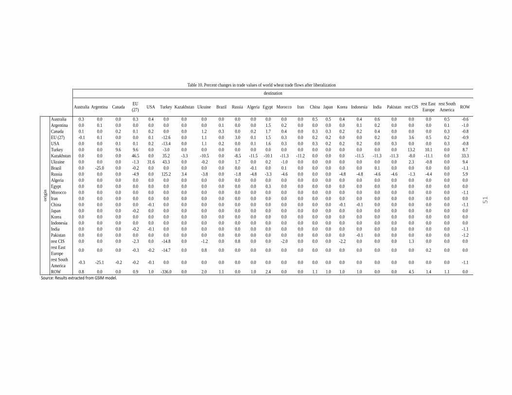
Australia Argentina CanadaEU

(27)USA Turkey Kazakhstan Ukraine Brazil Russia Algeria Egypt Morocco Iran China Japan Korea Indonesia India Pakistan rest CIS

rest East

Europe

rest South

AmericaROW

Australia 0.3 0.0 0.0 0.3 0.4 0.0 0.0 0.0 0.0 0.0 0.0 0.0 0.0 0.0 0.5 0.5 0.4 0.4 0.6 0.0 0.0 0.0 0.5 -0.6

Argentina 0.0 0.1 0.0 0.0 0.0 0.0 0.0 0.0 0.1 0.0 0.0 1.5 0.2 0.0 0.0 0.0 0.0 0.1 0.2 0.0 0.0 0.0 0.1 -1.0

Canada 0.1 0.0 0.2 0.1 0.2 0.0 0.0 1.2 0.3 0.0 0.2 1.7 0.4 0.0 0.3 0.3 0.2 0.2 0.4 0.0 0.0 0.0 0.3 -0.8

EU (27) -0.1 0.1 0.0 0.0 0.1 -12.6 0.0 1.1 0.0 3.0 0.1 1.5 0.3 0.0 0.2 0.2 0.0 0.0 0.2 0.0 3.6 0.5 0.2 -0.9

USA 0.0 0.0 0.1 0.1 0.2 -13.4 0.0 1.1 0.2 0.0 0.1 1.6 0.3 0.0 0.3 0.2 0.2 0.2 0.0 0.3 0.0 0.0 0.3 -0.8

Turkey 0.0 0.0 9.6 9.6 0.0 -3.0 0.0 0.0 0.0 0.0 0.0 0.0 0.0 0.0 0.0 0.0 0.0 0.0 0.0 0.0 13.2 10.1 0.0 8.7

Kazakhstan 0.0 0.0 0.0 46.5 0.0 35.2 -3.3 -10.5 0.0 -8.5 -11.5 -10.1 -11.3 -11.2 0.0 0.0 0.0 -11.5 -11.3 -11.3 -8.0 -11.1 0.0 33.3

Ukraine 0.0 0.0 0.0 -1.3 31.6 43.3 0.0 -0.2 0.0 1.7 0.0 0.2 -1.0 0.0 0.0 0.0 0.0 0.0 0.0 0.0 2.3 -0.8 0.0 9.4

Brazil 0.0 -25.0 0.0 -0.2 0.0 0.0 0.0 0.0 0.0 0.0 -0.1 0.0 0.1 0.0 0.0 0.0 0.0 0.0 0.1 0.0 0.0 0.0 0.0 -1.1

Russia 0.0 0.0 0.0 -4.9 0.0 125.2 3.4 -3.8 0.0 -1.8 -4.8 -3.3 -4.6 0.0 0.0 0.0 -4.8 -4.8 -4.6 -4.6 -1.3 -4.4 0.0 5.9

Algeria 0.0 0.0 0.0 0.0 0.0 0.0 0.0 0.0 0.0 0.0 0.0 0.0 0.0 0.0 0.0 0.0 0.0 0.0 0.0 0.0 0.0 0.0 0.0 0.0

Egypt 0.0 0.0 0.0 0.0 0.0 0.0 0.0 0.0 0.0 0.0 0.0 0.3 0.0 0.0 0.0 0.0 0.0 0.0 0.0 0.0 0.0 0.0 0.0 0.0

Morocco 0.0 0.0 0.0 0.0 0.0 0.0 0.0 0.0 0.0 0.0 0.0 0.0 0.0 0.0 0.0 0.0 0.0 0.0 0.0 0.0 0.0 0.0 0.0 -1.1

Iran 0.0 0.0 0.0 0.0 0.0 0.0 0.0 0.0 0.0 0.0 0.0 0.0 0.0 0.0 0.0 0.0 0.0 0.0 0.0 0.0 0.0 0.0 0.0 0.0

China 0.0 0.0 0.0 0.0 -0.1 0.0 0.0 0.0 0.0 0.0 0.0 0.0 0.0 0.0 0.0 0.0 -0.1 -0.1 0.0 0.0 0.0 0.0 0.0 -1.1

Japan 0.0 0.0 0.0 -0.2 0.0 0.0 0.0 0.0 0.0 0.0 0.0 0.0 0.0 0.0 0.0 0.0 0.0 0.0 0.0 0.0 0.0 0.0 0.0 0.0

Korea 0.0 0.0 0.0 0.0 0.0 0.0 0.0 0.0 0.0 0.0 0.0 0.0 0.0 0.0 0.0 0.0 0.0 0.0 0.0 0.0 0.0 0.0 0.0 0.0

Indonesia 0.0 0.0 0.0 0.0 0.0 0.0 0.0 0.0 0.0 0.0 0.0 0.0 0.0 0.0 0.0 0.0 0.0 0.0 0.0 0.0 0.0 0.0 0.0 0.0

India 0.0 0.0 0.0 -0.2 -0.1 0.0 0.0 0.0 0.0 0.0 0.0 0.0 0.0 0.0 0.0 0.0 0.0 0.0 0.0 0.0 0.0 0.0 0.0 -1.1

Pakistan 0.0 0.0 0.0 0.0 0.0 0.0 0.0 0.0 0.0 0.0 0.0 0.0 0.0 0.0 0.0 0.0 0.0 -0.1 0.0 0.0 0.0 0.0 0.0 -1.2

rest CIS 0.0 0.0 0.0 -2.3 0.0 -14.8 0.0 -1.2 0.0 0.8 0.0 0.0 -2.0 0.0 0.0 0.0 -2.2 0.0 0.0 0.0 1.3 0.0 0.0 0.0

rest East

Europe0.0 0.0 0.0 -0.3 -0.2 -14.7 0.0 0.8 0.0 0.0 0.0 0.0 0.0 0.0 0.0 0.0 0.0 0.0 0.0 0.0 0.0 0.2 0.0 0.0

rest South

America-0.3 -25.1 -0.2 -0.2 -0.1 0.0 0.0 0.0 0.0 0.0 0.0 0.0 0.0 0.0 0.0 0.0 0.0 0.0 0.0 0.0 0.0 0.0 0.0 -1.1

ROW 0.8 0.0 0.0 0.9 1.0 -336.0 0.0 2.0 1.1 0.0 1.0 2.4 0.0 0.0 1.1 1.0 1.0 1.0 0.0 0.0 4.5 1.4 1.1 0.0

Source:ResultsextractedfromGSIMmodel.

Table 10. Percent changes in trade values of world wheat trade flows after liberalization

ori

gin

destination

51

52

As is expected KRU, countries experience substantial changes in trade flows due to the

tariff reductions manifest in important importing markets. Russia experiences a large increase in

trade with Turkey, Kazakhstan, ROW and a marginal decrease in trade with the rest of the world

importers. Increase in export values from Russia to Turkey and ROW are due to tariff reductions.

The three percent increase in trade between Russia and Kazakhstan can not be attributed to tariff

reductions but rather to a big difference in changes in prices in Russia and Kazakhstan.

Ukraine’s value of exports to the US, Turkey and ROW increased by 32, 43 and 9 percent

respectively. There is also a marginal increase in trade with Russia, Egypt, the rest of the CIS as

well as slightly negative changes in trade with EU, Morocco and rest of Europe. This is due to

increased access to some markets and, hence, redistribution effects from one market to another.

Kazakhstan trades 47, 35 and 33 percent more with EU, Turkey and ROW respectively. These

changes also stem from tariff reductions. There is slightly less trade occurring with the rest of

Kazakhstan’s trading partners due to diversion of trade flows as a result of increased access in

other markets. It is also worth mentioning that the EU’s currently applied wheat import tariffs for

high quality wheat and medium or low quality wheat from WTO members is 0 and 95 euro per

ton. High quality wheat is identified as minimum 14 percent protein content while everything

else below 14 percent is considered medium or low quality wheat. In the future, as a result of

accession to the WTO, KRU country exporters might benefit from the absence of quotas for

“high quality wheat”.

The EU, the US, the rest of the CIS and the ROW have lower trade values with Turkey as

their relative market access conditions erode relative to the KRU countries in Turkish markets. In

general, major wheat exporting countries such as Argentina, Australia, Canada, the EU and the

US do not appear to be negatively impacted by KRU’s accession to the WTO to any important

53

degree. As their relative markets access conditions erode in the Turkish (for the EU and the US)

and ROW markets (these are mostly represented by Middle Eastern and African markets), their

trade flows are diverted and marginally distributed among other countries and regions at reduced

prices.

Trade diversion as a result of KRU countries’ obtaining improved access to markets has a

marginal impact on wheat output values as well. Table 11 provides changes in production. The

price changes as a result of the trade liberalization lead to changes in output produced. There is

an output decline in Australia, Argentina, Canada, the EU, the US, Turkey and the ROW as a

result of the decline in prices. The opposite is true for the countries experiencing higher prices for

wheat. The KRU countries respond to higher prices with more output. Countries such as Egypt

and the rest of the CIS experience increase in prices for domestic goods due to lower values of

imports and, as a result, produce more output.

54

Country percent in tonnes

original

production

in 2007 in

tonnes

Australia -0.16% -213 13569380

Argentina -0.05% -78 16486530

Canada -0.10% -203 20054000

EU (27) -0.06% -752 120263646

US -0.08% -442 55820400

Turkey -2.94% -5072 17234000

Kazakhstan 3.41% 5619 16466900

Ukraine 0.33% 457 13937700

Brazil -0.01% -3 4114060

Russia 1.40% 6917 49368000

Algeria -0.03% -7 2318960

Egypt 0.30% 225 7379000

Morocco 0.01% 2 1582630

Iran 0.04% 64 15886600

China 0.00% -38 109298296

Japan -0.01% -1 910100

Korea -0.02% 0 7351

Indonesia 0.00% 0 0

India 0.01% 73 75806700

Pakistan 0.01% 28 23294700

rest CIS 0.62% 847 13618304

rest East EUR 0.03% 23 6805676

rest South Am 0.00% -1 2987894

ROW -0.33% -1764 53993183

Table 11. Change in output percentage and value

Source:Results extracted from GSIM model and own

calculations

As can bee seen from Table 11, changes in output as a response to trade liberalization are,

in general, modest. Some countries produce more and some less. Just looking at the percentage

change can be deceiving, therefore percentage changes were reported in terms of tonnes.

Changes in production values are negligible when compared to the original production tonnage

recorded for 2007.

55

To ease the process of visualization of the results, KRU countries’ changes in trade flow

maps are provided in Appendix C. These maps were all generated using arc GIS22 software.

Once again, it is worth mentioning that the results should be analyzed with great caution

because they were generated by the partial equilibrium approach and not a general equilibrium

approach. Nevertheless, this research enhances the understanding of trade liberalization and

explains the possible outcomes of the KRU countries’ accession to the WTO.

6. 2 Sensitivity analysis

Sensitivity analysis was performed to ensure the robustness of the results over changes in

elasticity values. Assigning higher supply elasticities result in smaller producer price effects and

larger output effects. Altering the supply elasiticities across countries slightly changes the

magnitude of changes in consumer and producer welfare and as is predicted has no effect on the

direction (sign) of the changes.

Lower values of substitution eleasticities lead to lower quantity and price response, and

hence, lower welfare effects. Increasing these elasticity values does the opposite, but has no

effect on the direction of the changes. Results of the sensitivity analysis are provided in

Appendix B, Table 4 and Table 5.

22 Arc GIS is a geographic information system that allows to visualizes values, in our case, trade flows in terms of

American dollars.

56

6.3 Conclusion

The GSIM model was used to examine the impact of the KRU countries’ accession to the

WTO on world wheat trade. World wheat trade liberalization, reflecting the move to the MFN

tariff as a result of accession, was simulated. Accession to the WTO is expected to bring more

market access for KRU countries. Simulation results are consistent with the theory. Increased

access to markets leads to more trade between KRU countries and previously restricted markets.

KRU countries trade with now freer markets such as Turkey, the EU, China and the ROW

expands. Major traditional wheat exporters such as Australia, Canada, the EU, and the US do not

seem to be negatively impacted to any important degree from the accession of the KRU countries

to the WTO. Their relative market access conditions, however, erode in Turkish (for the EU and

the US) and ROW markets (these are mostly represented by Middle Eastern and African markets)

and their trade volumes are diverted and marginally distributed among other countries and

regions at reduced prices. Trade liberalization is not uniform across regions and, hence, leads to

different net welfare changes across countries. However, those welfare changes appear to be

modest.

Chapter 7 provides a discussion of the important findings and implications arising from

the simulation exercises.

57

Chapter 7: Important findings and implications

This thesis indicates that the accession of the KRU countries to the WTO can be expected

to result in observable changes in trade flows in the world wheat trade. Although net welfare

effects appear to be relatively small, there is a potential for intensification of trade among KRU

countries and their trade partners. Increases in the KRU’s countries’ export opportunities would

come at the expense of the other major wheat exporters such as Canada, the US, Australia and

the EU as their competitiveness erodes in several major importing markets (Turkey, the EU, and

the ROW). The loss, however, does not appear to be significant in terms of their dollar values.

Major exporters will be able to compensate the market access erosion by diverting and

distributing exports among other importing markets. Canada, the US, Australia and the EU’s

market presence is more diverse in terms of geography than that of the KRU region. These

countries hold an advantage in terms of transportation costs at this point in time. It is also

believed that these countries have established themselves as reliable exporters in contrast to KRU

countries. KRU countries have volatile production and are well known for their export bans.

Therefore, traditionally large exporters such as the US, Canada and Australia are less likely to

suffer as a result of the KRU’s accession to the WTO.

Accession to the WTO can bring market access opportunities for KRU countries.

Running scenarios with constrained supply elasticities among KRU countries did not alter the

end results in any significant way. It is, however, questionable whether producers can capitalize

on the opportunities provided by the WTO membership. This depends on factors such as future

productivity, domestic policies, adaptability to climate changes and other socio economic factors.

Infrastructure is one of the major constraints for KRU countries. Russia, Ukraine and Kazakhstan

58

are all putting considerable effort into improving the infrastructure for storing and transporting

grain, especially for access to remote markets. If KRU countries overcome their present

constraints and use their wheat producing resources efficiently, their presence in the world wheat

trade arena will remain strong and gain in prominence.

Considering the majority of the large trading nations are already part of the WTO, less

attention is given to the difference between the MFN and non-MFN tariffs. However, the later

difference appears to be substantial especially in trade of agricultural commodities. It is

important to note that the data on non–MFN tariffs is not easily accessible. WTO member

countries are not obligated to report their schedules on non-MFN tariffs. Thus, it takes a major

effort to compile non-MFN tariffs that are applied by member states of the WTO. No other

studies which used pre-accession tariff rates were found. Large files of tariff schedules for some

countries containing both MFN and non-MFN tariffs are accessible on the WTO website site.

Information provided on the online websites like TRAINS and MacMap are at times inconsistent

or provide MFN tariffs only.

59

Chapter 8: Conclusions

8.1 Summary of results

The WTO administers the agreed rules of international trade among 159 countries.

Countries join the WTO to become integrated into the modern global economy. One of the mort

important benefits that WTO membership provides is improved and more secure access to

member countries’ markets. Before enjoying the security provided by WTO membership, each

country wishing to join the WTO has to go through a four-stage accession process. After joining

the organization, countries are entitled to receive “most favored nation” treatment. It means,

among other things, that new members move from facing non-MFN tariffs to MFN tariffs which

all members of the WTO are extended.

World wheat is and likely will always be an important part of the global food basket.

Wheat is both relatively nonperishable in storage and transport making it an ideal commodity for

international movement. To date, wheat trade accounts for one third of the world grain trade and

this trade is expected to double by 2050 in response to the growing world population.

Black Sea wheat exporting countries are emerging as major exporters and producers of

wheat in the world. Their growing importance in world wheat trade has been evident since the

early 2000s. Growing wheat exports from this part of the world are due to several factors

including the collapse of the Soviet regime and its consequences in the agricultural sector. The

decline in livestock numbers, marginal increase in yields and favorable weather conditions are

believed to be the factors that contributed to the increase in wheat exports among KRU countries.

60

KRU countries have long wished to join the WTO. Negotiations for all three countries

were long and are still in progress for Kazakhstan. Ukraine was the first to become an official

member of the WTO in 2008, Russia joined in 2012 and Kazakhstan is expected to follow in the

near future.

As an important wheat producing region, accession of the KRU countries to the WTO is

expected to bring about important realignments in the world wheat trade flows as the countries

move from facing non MFN to MFN tariffs in the world import markets.

This empirical study employing a partial equilibrium, multi region GSIM model provided

useful insights into the implications of the accession of the KRU countries’ into the WTO. Major

exporting and importing countries (23 in total) including aggregated regions were included in the

research. A number of simulations of world wheat trade liberalization were carried out to assess

changes in world wheat trade flows, prices and changes in economic welfare. The results suggest

that KRU countries gain access and, therefore, increase export values to previously highly

protected markets such as the EU, Turkey, China and the ROW. More market access results in

higher prices for KRU countries. This will come at the expense of the traditional major exporters

such as the US, Australia, Canada and the EU. Losses as a result of the market access erosion for

these countries are small in financial terms. Their diversified presence in all markets across the

world allows them to divert and re-distribute their exports to other markets at slightly lower

prices. In short, accession to the WTO brings export opportunities for KRU countries with no

dramatic declines for the rest of the world. There are, of course, both losers and winners.

However, both net welfare losses and gains to the rest of the countries, however, appear to be

marginal. Major traditional wheat exporters will experience market access erosion in some

markets but are most likely to cope with this problem by selling more to other markets.

61

8.2 How it adds to the literature

This thesis investigates an important real event in the world’s wheat trade. Studies

relating to KRU countries trade in specific commodities are scarce and largely descriptive. A

study of world wheat trade liberalization carried out by Gomez-Plana and Devadoss (2004)

pursues similar question, but fails to mimic the real world wheat trade scenario. The authors

assume complete removal of all bilateral tariffs across all major wheat importing and exporting

countries. Complete removal of trade barriers is, however, unlikely. In addition, Gomez-Plana

and Devadoss (2004) did not differentiate between MFN versus non-MFN tariffs and appear to

arrive at the average between the two.

This study contributes to the general understanding of the increasing importance of wheat

exporters from the Black Sea region in world wheat trade. It provokes further discussions related

to the accession of the KRU countries into the WTO.

8.3 Limitations of the Study

Limitations of this study can be divided into two categories: those that are attributable to

the GSIM model and those specific to this study. This research utilizes GSIM model approach to

assess the effects of the trade liberalization. Although the model has significant advantages, it

also has a number of limitations that should be kept in mind. Firstly, it is worth remembering that

GSIM’s partial equilibrium approach belies its focus on only part of the total economy. It means

that the model does not account for intersectoral linkages and possible income or resource re-

allocation effects throughout the whole economy. Therefore, changes in the rest of the economy

are not accounted for by the GSIM. This implies that the results of the trade liberalization

scenarios might be under or overestimated. Secondly, the GSIM model is a static model that

62

compares scenarios at a given point in time. It does not allow for long term adjustments or

transition periods that allow for dynamic economic effects. Thirdly, the model assumes full price

transmissions. However changes in border prices might not be fully transmitted to producers and

households, hence, actual responses to reforms might differ in reality from those projected by the

analysis. Finally, the assumptions made with regard to the elasticity values may be a limitation.

Values assigned across regions might not be accurate in reflecting the responsiveness to the price

changes. The model is based on the representative agent assumption that does not differentiate

between various groups within a particular region. The responsiveness to the price is kept the

same among all of them.

The GSIM model analysis is based on the observed volumes of bilateral trade at a certain

time. It captures the responses to trade liberalization between countries that are trade partners,

but does not capture possible “new trade” that can potentially occur between non trading partners

after the reduction of restrictive tariff rates. In order to address this shortcoming, the value of

one dollar was recorded to trade values that were equal to zero to allow for positive trade

responses where tariff changes are substantial23.

Another major limitation specific to this study is lack of data. The production and export

subsidies data are not included to the model. Therefore, this study is not inclusive of non-tariff

based trade distorting factors that could shed more light on the effects of KRU countries

accession to the WTO.

23 For example, China and Kazakhstan is not reported as trading in 2007. However, since the difference in China’s

MFN vs non MFN tariffs is large, another model run was performed to test for this shortfall. Initial trade volumes

from KRU-China were altered from zero values to one dollar (see chapter 6)

63

8.4 Areas of Future Research

Future research can potentially address the shortcoming of the present study. Most

importantly, future studies should focus on trade distorting instruments such as industry specific

production subsidies. Agricultural subsidization is one of the most difficult topics in the WTO. It

is expected that the existing agricultural subsidies will be reduced following the accession to the

WTO. However, developing countries accessing the WTO are given a transition period to lower

the levels of agricultural support. Of course, not all types of subsidization are prohibited by the

WTO regulations. The WTO regulations distinguish three types of support policies that are

classified under three color boxes: green, blue and red24.

For example, major wheat exporting countries such as Canada, the US and Australia have

already expressed concerns regarding the level of transport subsidization for wheat exports,

particularly in Kazakhstan. These transportation subsidies are most likely classified under the

red box. As is suggested by the name “red box”, these subsidies are prohibited by the WTO.

Kazakhstan officials are using the “landlocked” argument and focusing on retaining a transition

period.

In short, agricultural support policies are important in international trade. Therefore the

inclusion of other trade distorting measures such as subsidization can yield more revealing

insight into the effects of the accession to the WTO.

The shortcomings embedded in the modeling approach could be improved by the

development of a new modeling initiative that would require considerable effort and time.

Researchers could expand the scope of the existing general equilibrium models to assess the

24 A more detailed discussion on the WTO regulations regarding support policies can be obtained from WTO (2010)

64

economy wide effects of the accession of the countries to the WTO and the ramifications for

agriculture in general. The general equilibrium approach is data intensive yet could be carried out

successfully given enough time and resources.

8.5 Conclusion

The contribution of this thesis includes an assessment of world wheat trade liberalization

following the accession of the Black Sea region exporters into the WTO. It measures the effects

of trade liberalization on world wheat trade flows, prices and economic welfare across different

exporting and importing regions. Although, the thesis is limited by the exclusion of non-tariff

based measures due to lack of data, the research provides insights to the changes that may be

expected in world wheat trade. The thesis differs from other studies because it uses a partial

equilibrium approach to explore a real world case rather than a hypothetical issue. Further, the

thesis provided a discussion regarding the global trade in wheat, the KRU countries’ emergence

in the world wheat markets and their accession to the WTO. This thesis indicates that increased

access to world markets as a result of accession to the WTO brings export opportunities for KRU

countries at no major loss to other traditional exporters. Whether the Black Sea region exporters

will be able to capitalize on the opportunity is, nevertheless, questionable and, hence, as is what

the future holds.

65

References

ABARE (1996). The MEGABARE model: Interim Documentation. Canberra, Australian Bureau

of Agriculture and Resource Economics.

Armington, Paul, S. (1969). A Theory of Demand for Products Distinguished by Place of

Production. Vol. 16. Washington: International Monetary Fund.

Babkin, K.A, Kuznecov A. B, E. A Korchevoi, V. V Pronin, and V. A Samohvalova (2012).

Consequances of Russia's Accession to the WTO. WTO inform , Moscow: WTO inform.

Bacchetta, M., C. Beverelli, O. Cadot, M. Fugazza, J-M. Grether, M. Helble, A. Nicita, R.

Piermartini (2012). A Practical Guide to Trade Policy Analysis. Geneva: UNCTAD and the

WTO.

Baltinfo, n.d. Logistics Problems Hamper Russian Grain Exports (translation from russian).

http://www.baltinfo.ru/2009/12/18/Problemy-logistiki-meshaiut-eksportu-rossiiskogo-zerna-

120835 (accessed March 12, 2013).

Bank, World. Bilateral Tariff Data. World Bank. econ.worldbank.org.

Benirschka, M, and W.W Koo (1995). World Wheat Policy Simulation Model: Description and

Computer Program Documentation. Department of Agricultural Economics. Fargo: North

Dakota State University.

Boersch, M. (2013) Pulse Production in Ukraine Russia and Kazakhstan. Presentation For SPG,

Saskatoon Mercantile Consulting Venture Inc., Winnipeg, Canada.

Devadoss, S., M. Helmar, and W. H. Meyers (1990). The World Wheat Trade Model:

Specification, Estimation, and Validation. Vols. Technical Report 90-TR14. Center for

Agrculture and Rural Development. Ames, Iowa: Iowa State University.

Dumans, T, and D Nivet (2003). Perception of Black Sea Wheat by European Users: What

competition for French wheat? Paris: Ecole Superieur d'Agriculture d'Angers.

FAO n.d. "FAO Cereal Supply and Demand Brief." Rome: Food and Agriculture Organization.

www.fao.org/worldfoodsituation/wfs-home/csbd/en/ (accessed April 2, 2013).

FAO, 2003. World Agriculture Towards 2015/2020. Edited by Jelle Bruinsma. London: Food

and Agriculture Organization.

FAOSTAT n.d. FAOSTAT. Animal Production. www.faostat.fao.org (accessed March 29, 2013).

FAOSTATa n.d. FAOSTAT.Cereal Production. Yeild Information. faostat3.fao.org (accessed

April 1, 2013).

66

Felix, Kogan (1981). "Grain production on the USSR. Present Situation, Perspectives for

Development and Methods for Prediction." Staff Report, Washington: United States Department

of Agriculture.

Fellmann, Thomas, and Olexandr Nekhay (2012). Agricultural Sector and Market

Developements: a Special Focus on Ukraine, Russia and Kazakhstan. European Commission

Join Research Centre Institute for Prospective Technological Studies, Luxembourg: European

Commission.

Francois, J.F., and H.K Hall (2003). Global Simulation Analysis of Industry-Level Trade Policy.

Tinbergen Institute, CERP, Washington: US Commerce Department.

Fukita, M, P Krugman, and A Venables (2000). The Spacial Economy- Cities, Regions and

International Trade. Cambridge, MA; MIT Press.

Gomez-Plana, A., and S Devadoss (2004). A spatial Equilibrium Analysis of Trade Policy

Reforms on The World Wheat Markets. Applied Economics, 36 (15): 1643-1648.

Hertel, T. (1997). Global Trade Analysis: Modeling and Applications. Cambridge University

Press.

Holzner, Mario (2008). GSIM Measurment of the Effects of the EU accession of the Balkans and

Turkey on Agricultural Trade. South East European Journal of Economics and Business 3 (1): 7-

14 .

Holzner, Mario, and F Peci (2012). "Measuring the Effects of Trade Liberalization in Kosovo."

Vienna: The Vienna Institute for International Economic Studies.

Inmaculada, Martinez-Zarzosa, and Suarez-Burguet Celestino (2005). Transport Costs and Trade:

Empirical Evidence for Latinoamerican Imports From the European Union. Journal of

International Trade and Economic Development, 14 (3): 353-371.

Ivus, Olena, and Aaron Strong (2007). Modeling Approaches to the Analysis of Trade Policy:

Computable General Equilibrium and Gravity Models. In Handbook on Internaitonal Trade

Policy, William Kerr and James Gaisford, (eds.). Cheltenham: Edward Elgar Publishing Limited,

pp 44-54.

Jammes, Olivier, and Marcelo Olarreaga (2005). Explaininf SMART and GSIM. Washington: The

World Bank .

Kee, Hiau Looi, A Nicita, and M Olarreaga (2004). Import Demand Elasticities and Trade

Distortions. The Review of Economics and Statistics 90 (4): 666-682.

67

Leudjou, Roland (2012). The Doha Round and Food Security in the Dairy Sector in Cameroon:

A Global Simulation Model (GSIM) Approach. The Estey Centre Journal of International Law

and Trade Policy 13 (1) : 115-130.

Liefert, Olga, William Liefert, and Eric Luebenhusen (2013). Rising Grain Exports by the

Former Soviet Union Region. Washington: United States Department of Agriculture.

MacMap n.d. macmap.org. Geneva: International Trade Center.

Meyers, William, H., Patrick Westhoff, Jacinto Fabiosa, and Dermot, J. Hayes (2010). "The

FAPRI Global Modeling System and Outlook Porcess." Journal of International Agricultural

Trade and Developement 6 (1): 1-19.

Mutambatsere, Emily (2006). Trade Policy Reforms in the Cereals Sector of the SADC Region:

Implication on Food Security. Department of Applied Economics and Managment. Cornell

University. Ithaca: Cornell University.

Nicita, A, and M Olarreaga (2006). Trade, Production and Protection Database 1974-2004.

World Bank Econ Review 21 (1): 165-171.

OECD-FAO (2012). OECD-FAO Agricultural Outlook 2012-2021 Database. OECD Statistics

website. June 2012. http://stats.oecd.org/index.aspx?Queryld=23336 (accessed April 18, 2013).

Prikhodko, Dmitri (2009). Grain Markets in Kazakhstan, Russia and Ukraine. New York: FAO.

Pugachev, N (2012). Ukraine's Accession to the WTO: Accession Conditions. Presentation.

Moscow: Ministry of Agriculture of Russia Training Centre.

Roningen, V., D. Praveen, and J. Sullivan (1991). Documentation of the Static World Policy

Simulation (SWOPSIM) Modeling Framework. Economics and Research Service. Staff Report

No. AGES 9151. Washington: US Department of Agriculture.

Russian Federation Federal State Statistics Service. Agriculture. Livestock. www.gks.ru

(accessed April 12, 2013).

Serletis, George, and James Fetzer (2008). Modeling the Impact of the US Tobacco Quota Buyout.

Working Paper No 2008-06-A. Washington: US International Trade Commission.

State statistics services of Ukraine. Stock-breeding. www.ukrstat.gov.ua (accessed March 28,

2013).

Statistics Agency of Kazakhstan n.d. Agriculture. Cattle and bird livestock. www.eng.stat.kz

(accessed March 1, 2013).

Takayama, T, and G. G. Judge (1971). Spatial and Temporal Price and Allocation Models.

Amsterdam: North Holland Publishing Co.

68

TAO n.d. WTO: Tariff Analysis online. tariffanalysis.wto org.

Tariffdata n.d. tariffdata.wto.org. WTO.

Tongeren, F. W., H. Neijl, and Y. Surry (2001). Global Models Applied to Agricultural and

Trade Policies: A Review and Assessment. Agricultural Economics 26 (2): 149-172.

Trademap n.d. www.trademap.org. Geneva: International Trade Center.

UN Department of Economic and Social Affairs, Population Division (2011). World Population

Prospects: The 2010 Revision. CD-ROM Edition. United Nations Department of Economic and

Social Affairs. New York: United Nations. esa.un.org/wpp/ Excel-Data/population.htm (accessed

April 14, 2013).

US Census Bureau, n.d. International Programs. World Population 1950-2050.

http://www.census.gov (accessed November 29, 2012).

USDAa, n.d USDA Wheat Baseline, 2012-21. www.ers.usda.gov (accessed March 21, 2013).

USDA (2013). FAS Production, Supply and Distribution Online (USDA PS&D).

http://www.fas.usda.gov/psdonline/ (accessed January 17, 2013).

USDA, n.d. Trade.World wheat maret. http://www.ers.usda.gov (accessed January 1, 2013).

USITC (2004). The US Applied eneral Equilibrium Model. Vols. Note No. 2004-01-A. US

Office of Economic Research. Washington: International Trade Commission.

Vanzetti, D., S. Fernandez, and V Chau (2005). Banana Split: How EU Policies Devide Global

Producers. Vol. 31. Policy Issues in International Trade and Commodities Study Series. New

York and Geneva: United Nations.

Vanzetti, David, and Ralf Peters (2004). "User Manual and Handbook on Agricultural Trade

Policy Simulation Model." Policy Issues in International Trade and Commodities Study Series

No. 24. Geneva: United Nations Conference on Trade and Development.

Vassilieva, Y, and Levin Flake (2011). Overview of Russian Grain Port Capacity and

Transportation. GAIN report N:RS1149, Washington: United States Department of Agriculture.

Wandel, J. (2008) Agroholdings ot clusters in Kazakhstan's Agri-Food Sector? Almaty: German-

Kazakh University.

Weigand, Chad (2011). Wheat Import Projections Towards 2050. Arlington: US Wheat

Associates.

WITS. World Trade Integrated Solutions. Washington: World Bank. www.wits.worldbank.org.

69

Worz, J, O Pindyuk, M Holzner, and V Astrov (2008). "Russia's WTO accession in the Meduim

and Long Run-A Global Simulation Model (GSIM) approach." Vienna: The Vienna Institute for

International Economy.

WTO (1996). Accession of the Republic of Kazakhstan: Memorandum on the Foreighn Trade.

Geneva: World Trade Organization.

WTO Information and External Relations Devision (2011). Understanding the WTO Fiftth

Edition. Geneve: World Trade Organization.

WTO n.d. Ten Benefits of the WTO Trading System.

http://www.wto.org/english_e/whatis_e/10ben_e/10b00_e.htm (accessed May 1, 2013).

WTO (2010). Understanding the WTO Fifth Edition. Edited by World Ttade Organization

Information and External Relations. Geneva: World Trade Organization.

Appendix A

Figure 1. Map of KRU’s exit routes to the world markets

Existing routs

Future routs

70

71

Australia EU(27) is: rest CIS is: rest East Europe is: rest South America is:

Argentina Belgium Armenia Croatia Bolivia

Canada Bulgaria Azerbaijan Serbia Chile

Eu(27) Czech Republic Belarus Montenegro Colombia

US Denmark Kyrgyzstan Bosnia Ecuador

Turkey Germany Moldova Herzigovina Guyana

Kazakhstan Estonia Tajikistan Albania Paraguay

Ukraine Ireland Uzbekistan Kosovo Peru

Brazil Greece Turkmenistan Macedonia Suriname

Russia Spain Uruguay

Algeria France Venezuela

Egypt Italy

Morocco Cyprus

Iran Latvia

China Lithuania

Japan Luxembourg

Korea Hungary

Indonesia Malta

India Netherlands

Pakistan Austria

rest CIS Poland

rest East Eur Portugal

rest South Am Romania

ROW Slovenia

Slovakia

Finland

Sweden

United Kingdom

Table 1. List of countries included in the model

72

Composite Demand

Australia -2.49

Argentina -2.52

Canada -2.29

Eu(27)* -3

US -3.39

Turkey -1.97

Kazakhstan* -1.46

Ukraine -1.46

Brazil -3.38

Russia* -2

Algeria -1.59

Egypt -1.78

Morocco -1.45

Iran -1.87

China -2.54

Japan -4.05

Korea -2.08

Indonesia -2.09

India -3.26

Pakistan* -1.25

rest CIS* -1.25

rest East Eur* -1.25

rest South Am* -1.5

ROW* -1.5

From: Kee, Nicita and Ollareaga (2004)

* approximations

Table 2. Aggregate Import demand

elasticities

73

Appendix B

The three tested scenarios lead only to marginally different results. Different supply

elasticity values for KRU countries had an only small impact on the outcome. Hence, main

discussions of results were based upon scenario 1 outcomes.

Assigning different supply elasticities for KRU countries is as a crude proxy for potential

differences in transition economies’ ability to respond to price changes compared to modern

market economies. First scenario assumes that the wheat industry in Russia, Ukraine and

Kazakhstan (RUK) are able to respond to changes in demand to a similar degree as the industry

in modern market economies. Therefore, the three countries take the export supply elasticity

value of 1.5 (as with the rest of the major wheat export suppliers). Second scenario assumes that

RUK are less responsive to demand changes. In this case, RUK were each assigned export supply

elasticity of value 0.5. Third scenario, where KRU countries are each assigned export supply

elasticity values equal to zero, is a worst-case scenario that assumes KRU countries are not able

to respond to any degree to changes in prices.

Producer

surplus

Consumer

surplus

Tariff

revenue

Change in

subsidy

payments

Net welfare

effect

Change in

Overall

Consumer

Prices

Change in

Output

Producer

Price for

Home Good

Market

Price for

Home Good

Kazakhstan 72003.7 -44908.1 0.0 0.0 27095.7 2.27% 3.4% 2.27% 2.27%

Ukraine 5492.6 -5919.9 0.7 0.0 -426.6 0.25% 0.3% 0.22% 0.22%

Russia 116093.1 -84017.7 0.7 0.0 32076.1 0.95% 1.4% 0.93% 0.93%

Kazakhstan 71198.5 -44908.1 0.0 0.0 26290.5 2.27% 3.4% 2.27% 2.27%

Ukraine 5486.6 -5919.9 0.7 0.0 -432.6 0.25% 0.3% 0.22% 0.22%

Russia 115554.7 -84017.7 0.7 0.0 31537.7 0.95% 1.4% 0.93% 0.93%

Kazakhstan 70795.9 -44908.1 0.0 0.0 25887.9 2.27% 3.4% 2.27% 2.27%

Ukraine 5483.6 -5919.9 0.7 0.0 -435.6 0.25% 0.3% 0.22% 0.22%

Russia 115285.5 -84017.7 0.7 0.0 31268.4 0.95% 1.4% 0.93% 0.93%

Source: extracted from the GSIM model results

Table 1. Summary of Effects

welfare (in 1000 dollars) other (in %)

scenario2

scenaario 3

scenario 1

74

Table 1. provides a brief comparison of the three scenarios. Export supply elasticity of

value 0.5 in Scenario 2, resulted in slightly lower value of producer surplus across KRU

countries and, hence, lower values of net welfare effects in Kazakhstan and Russia as well as a

marginal increase in Ukraine’s negative net welfare effects. The magnitude of changes, however,

appears to be negligible. Scenario 3, where export supply elasticity is equal to zero across KRU

countries, yields lower producer surplus values than in all previous two scenarios. Once again,

these changes appear to be very small. Changes in prices were insufficient to produce any

changes in other results values rounded at ten digit level25.

The model was, however, tested for the responsiveness to changes in supply elasticities

and yielded theoretically consistent results.

Sensitivity analysis was performed and reported in Table 2 and 3 of the Appendix B.

25 The difference in price changes across three scenarios was negligible to the extent that no discernible impact on

trade flows was detected given the degree of rounding built into the GSIM model.

75

Sensitivity analysis was performed to ensure the robustness of the results over changes in

elasticity values. Table 3 reports sensitivity analysis results with respect to export supply

elasticities. Assigning higher supply elasticities result in smaller producer price effects and larger

output effects. Altering the supply elasiticities across all countries slightly changes the magnitude

of changes in consumer and producer welfare and, as is predicted, has no effect on the direction

(sign) of the changes.

Producer

surplus

Consumer

surplus

Tariff

revenue

Change in

subsidy

payments

Net welfare

effect

Change in

Overall

Consumer

Prices

Change in

Output

Producer

Price for

Home Good

Market

Price for

Home Good

A B C D E= A+B+C+D percent percent percent percent

Australia -3077.8 1530.2 0.0 0.0 -1547.5 -0.10% -0.2% -0.10% -0.10%

Argentina -994.0 393.9 14.1 0.0 -586.0 -0.03% -0.1% -0.03% -0.03%

Canada -3090.8 371.5 0.2 0.0 -2719.1 -0.06% -0.1% -0.06% -0.06%

EU27 -10624.9 24062.1 -21974.9 0.0 -8537.7 -0.09% -0.1% -0.04% -0.04%

US -7014.4 3380.1 -141.3 0.0 -3775.6 -0.05% -0.1% -0.05% -0.05%

Turkey -105538.9 303962.6 21856.2 0.0 220279.9 -4.05% -3.5% -1.75% -1.75%

Kazakhstan 64178.8 -39831.5 0.0 0.0 24347.4 2.02% 4.0% 2.02% 2.02%

Ukraine 4689.6 -5085.0 0.6 0.0 -394.8 0.21% 0.4% 0.19% 0.19%

Brazil -51.2 480.9 16.7 0.0 446.4 -0.02% 0.0% 0.00% 0.00%

Russia 103918.1 -75022.6 0.6 0.0 28896.1 0.84% 1.7% 0.84% 0.84%

Algeria -55.6 561.8 0.0 0.0 506.1 -0.04% 0.0% -0.02% -0.02%

Egypt 1505.6 -10164.6 0.0 0.0 -8659.0 0.36% 0.3% 0.17% 0.17%

Marocco 9.5 -115.6 0.0 0.0 -106.0 0.01% 0.0% 0.01% 0.01%

Iran 433.5 -982.4 -224.3 0.0 -773.2 0.05% 0.0% 0.02% 0.02%

China -464.1 466.3 19.2 0.0 21.4 0.00% 0.0% 0.00% 0.00%

Japan -10.8 643.1 122.1 0.0 754.4 -0.05% 0.0% -0.01% -0.01%

Korea -0.3 182.7 1.0 0.0 183.4 -0.03% 0.0% -0.01% -0.01%

Indonesia 0.0 219.7 5.1 0.0 224.8 -0.03% 0.0% 0.00% 0.00%

India 1404.1 -5812.6 -5851.0 0.0 -10259.6 0.02% 0.0% 0.01% 0.01%

Pakistan 405.9 -984.0 -212.0 0.0 -790.2 0.01% 0.0% 0.01% 0.01%

rest CIS 3635.7 -12865.4 3.4 0.0 -9226.3 0.78% 0.6% 0.32% 0.32%

rest East Europe 63.3 -530.1 -573.2 0.0 -1040.0 0.07% 0.0% 0.02% 0.02%

rest South America -816.7 1608.5 143.6 0.0 935.4 0.00% 0.0% 0.00% 0.00%

ROW -25186.9 81240.9 -58012.3 0.0 -1958.3 -0.32% -0.4% -0.20% -0.20%

Source: Results extracted from GSIM model

Table 2. Sensativity analysis. Higher values of supply elasticities(increase by 0.5 across all countries)

Summary of Effects

welfare other

76

Table 4 provides a sensitivity analysis results with respect to elasticities of substitution.

Lower values of substitution elasticities lead to lower quantity and price response, and hence,

lower welfare effects. Increasing these elasticity values does the opposite, but has no effect on

the direction of the changes.

Producer

surplus

Consumer

surplus

Tariff

revenue

Change in

subsidy

payments

Net welfare

effect

Change in

Overall

Consumer

Prices

Change in

Output

Producer

Price for

Home Good

Market

Price for

Home Good

A B C D E= A+B+C+D percent percent percent percent

Australia -560.2 278.0 0.0 0.0 -282.2 -0.02% 0.0% -0.02% -0.02%

Argentina -170.6 52.0 16.9 0.0 -101.7 0.00% 0.0% 0.00% 0.00%

Canada -508.4 61.0 0.0 0.0 -447.4 -0.01% 0.0% -0.01% -0.01%

EU(27) 3010.9 14157.9 -20572.6 0.0 -3403.9 -0.06% 0.0% 0.01% 0.01%

US -1198.8 713.9 -153.3 0.0 -638.2 -0.01% 0.0% -0.01% -0.01%

Turkey -1380.5 194694.4 -86921.6 0.0 106392.2 -2.63% 0.0% -0.02% -0.02%

Kazakhstan 38745.2 -24395.5 0.0 0.0 14349.8 1.24% 1.9% 1.24% 1.24%

Ukraine 2283.9 -2552.9 0.0 0.0 -269.0 0.11% 0.1% 0.09% 0.09%

Brazil 11.0 62.6 1.1 0.0 74.7 0.00% 0.0% 0.00% 0.00%

Russia 60248.9 -43753.2 0.0 0.0 16495.7 0.49% 0.7% 0.49% 0.49%

Algeria 1.6 -65.4 0.0 0.0 -63.8 0.00% 0.0% 0.00% 0.00%

Egypt 109.0 -5383.2 0.0 0.0 -5274.1 0.19% 0.0% 0.01% 0.01%

Morocco 8.1 -316.6 0.0 0.0 -308.5 0.03% 0.0% 0.00% 0.00%

Iran 12.9 -350.8 -35.1 0.0 -373.0 0.02% 0.0% 0.00% 0.00%

China -52.8 53.9 0.9 0.0 2.0 0.00% 0.0% 0.00% 0.00%

Japan 7.3 101.4 17.9 0.0 126.6 -0.01% 0.0% 0.00% 0.00%

Korea 0.0 31.0 0.1 0.0 31.1 -0.01% 0.0% 0.00% 0.00%

Indonesia 0.0 -23.3 -0.4 0.0 -23.7 0.00% 0.0% 0.00% 0.00%

India -683.9 -1954.1 -911.9 0.0 -3549.8 0.01% 0.0% 0.00% 0.00%

Pakistan 59.2 -410.2 -32.2 0.0 -383.2 0.01% 0.0% 0.00% 0.00%

rest CIS 915.3 -6604.6 0.3 0.0 -5689.0 0.40% 0.1% 0.08% 0.08%

rest East Europe 49.2 -477.7 -82.7 0.0 -511.2 0.06% 0.0% 0.01% 0.01%

rest South America -39.2 179.1 6.6 0.0 146.4 0.00% 0.0% 0.00% 0.00%

ROW -9135.0 67465.2 -60882.1 0.0 -2551.8 -0.26% -0.1% -0.07% -0.07%

Table 3. Sensativity analysis. Lower values of substitution elasticities (equal to 2 across all countries)

Summary of Effects

welfare other

Source: Results extracted from GSIM model

Appendix C

77

78

79

80

The maps above were generated to the ease the visualization of the results. They were all

generated using GIS software. Each map presents the changes in trade flows between KRU

countries and their export destinations. Increases or decreases in trade is represented by green and

pink colours respectively.

Countries and regions with no colouration represent no or very small change in quantities

traded. The most important changes in trade flows are also indicated with callout boxes.