Accelerating Roundabout Implementation in the United States – Volume III of VII

Assessment of the Environmental Characteristics of Roundabouts

PUBLICATION NO. FHWA-SA-15-071 SEPTEMBER 2015

i

FOREWORD Since the Federal Highway Administration (FHWA) published the first Roundabouts Informational Guide in 2000, the estimated number of roundabouts in the United States has grown from fewer than one hundred to several thousand. Roundabouts remain a high priority for FHWA due to their proven ability to reduce severe crashes by an average of 80 percent. They are featured as one of the Office of Safety Proven Safety Countermeasures and were included in the Every Day Counts 2 campaign for Intersection & Interchange Geometrics.

As roundabouts became more common across a wide range of traffic conditions, specific questions emerged on how to further tailor certain aspects of their design to better meet the needs of a growing number and diversity of stakeholders. The substantial work performed for this project – Accelerating Roundabout Implementation in the United States – sought to address several of the most pressing issues of National significance, including enhancing safety, improving operational efficiency, considering environmental effects, accommodating freight movement and providing pedestrian accessibility. This work represents yet another notable step forward in advancing roundabouts in the United States.

The electronic versions of each of the seven report volumes that document this project are available on the Office of Safety website at http://safety.fhwa.dot.gov/.

Michael S. Griffith Director Office of Safety Technologies

NOTICE This document is disseminated under the sponsorship of the U.S. Department of Transportation in the interest of information exchange. The U.S. Government assumes no liability for the use of the information contained in this document. This report does not constitute a standard, specification, or regulation.

The U.S. Government does not endorse products or manufacturers. Trademarks or manufacturers’ names appear in this report only because they are considered essential to the objective of the document.

QUALITY ASSURANCE STATEMENT The Federal Highway Administration (FHWA) provides high-quality information to serve Government, industry, and the public in a manner that promotes public understanding. Standards and policies are used to ensure and maximize the quality, objectivity, utility, and integrity of its information. FHWA periodically reviews quality issues and adjusts its programs and processes to ensure continuous quality improvement.

ii

TECHNICAL REPORT DOCUMENTATION PAGE 1. Report No. FHWA-SA-15-071

2. Government Accession No. 3. Recipient’s Catalog No.

4. Title and Subtitle Accelerating Roundabouts in the U.S.: Volume III of VII - Assessment of the Environmental Characteristics of Roundabouts

5. Report Date September 2015 6. Performing Organization Code:

7. Author(s) K. Salamati1, N. Rouphail1, C. Frey1, B. Schroeder1 and L. Rodegerdts2

8. Performing Organization Report No. 11861 Task 4

9. Performing Organization Name and Address 1Institute for Transportation Research and Education North Carolina State University, Centennial Campus, Box 8601, Raleigh, North Carolina 27695-8601 U.S.A 2Kittelson & Associates, Inc., 610 SW Alder St., Suite 700, Portland, OR 97205

10. Work Unit No. (TRAIS) 11. Contract or Grant No. DTFH61-10-D-00023-T-11002

12. Sponsoring Agency Name and Address Office of Safety Federal Highway Administration United States Department of Transportation 1200 New Jersey Avenue SE Washington, DC 20590

13. Type of Report and Period Covered Technical Report August 2011 through September 2015

14. Sponsoring Agency Code FHWA HSA

15. Supplementary Notes The Contracting Officer’s Technical Manager (COTM) was Jeffrey Shaw, HSST Safety Design Team 16. Abstract This volume is third in a series of seven. The other volumes in the series are: Volume I – Evaluation of Rectangular Rapid‐Flashing Beacons at Multilane Roundabouts, Volume II – Assessment of Roundabout Capacity Models for the Highway Capacity Manual Final Report, Volume IV – A Review of Fatal and Severe Injury Crashes at Roundabouts, Volume V – Evaluation of Geometric Parameters that Affect Truck Maneuvering and Stability, Volume VI – Investigation of Crosswalk Design and Driver Behaviors, and Volume VII – Human Factor Assessment of Traffic Control Device Effectiveness. These reports document a Federal Highway Administration (FHWA) project to investigate and evaluate several important aspects of roundabout design and operation for the purpose of providing practitioners with better information, leading to more widespread and routine implementation of higher quality roundabouts.

This research sought to develop a simple methodology for estimating pollutant emissions generated at roundabouts and comparing them to those generated at signalized intersections. The premise for this research is that the environmental performance is tied to the operational performance of the roundabout, with emission levels being sensitive to levels of traffic volume and congestion. The research resulted in empirically-based vehicle activity models and emissions models for roundabouts and signalized intersections. The activity models take into account driver behavior, traffic conditions and infrastructure design, and were produced under consideration of three trajectory types though the intersections as a function of the demand volume and, when appropriate, signal timing. The emissions models were based on Portable Emissions Measurement System (PEMS) data, and consider vehicle specific power (VSP) distributions for vehicles measured at roundabouts and signalized intersections. Combining the two models via the VSP approach resulted in emission estimates near the intersections at various temporal and spatial scales. All models are macroscopic in nature and were implemented in a spreadsheet-based emissions computational engine. The analysis approach is most suitable in a planning-level assessment of roundabouts in relation to traffic signals. Results indicate that emissions rates at roundabouts tended to be lower than those at intersections (1) for demand-to-capacity (d/c) ratios less than 0.7, (2) for higher d/c ratios if signal progression at the intersections was poor, and (3) in general for oversaturated periods. 17. Key Words Roundabouts, traffic signal, operations, environmental, emissions, vehicle specific power, congestion

18. Distribution Statement No restrictions. This document is available to the public at http://safety.fhwa.dot.gov/

19. Security Classif. (of this report) Unclassified

20. Security Classif. (of this page) Unclassified

21. No. of Pages 81

22. Price

Form DOT F 1700.7 (8-72) Reproduction of completed page authorized

iii

TABLE OF CONTENTS

FOREWORD.................................................................................................................................. i NOTICE .......................................................................................................................................... i QUALITY ASSURANCE STATEMENT ................................................................................... i TABLE OF CONTENTS ............................................................................................................ iii LIST OF FIGURES ...................................................................................................................... v

LIST OF TABLES ..................................................................................................................... viii CHAPTER 1. INTRODUCTION ............................................................................................... 1

BACKGROUND ....................................................................................................................... 1

OBJECTIVE ............................................................................................................................. 3

CHAPTER 2. LITERATURE REVIEW ................................................................................... 5

CHAPTER 3. METHODOLOGY .............................................................................................. 7

CHAPTER 4. RESULTS ........................................................................................................... 11

ACTIVITY MODELS ............................................................................................................ 11

Speed Profiles ...................................................................................................................... 11

Trajectory Profile Frequency ............................................................................................ 13

Roundabout Profiles ........................................................................................................ 13

Signalized Intersections ................................................................................................... 16

Emissions Estimation .......................................................................................................... 19

Vehicle Specific Power and Vehicle Emission Rates ..................................................... 19

Generating Representative VSP Distributions ................................................................ 22

Intersection Approach Emission Estimation Method Using VSP ................................. 26

CHAPTER 5. IMPLEMENTATION ....................................................................................... 29

CASE STUDY INPUT PARAMETERS ............................................................................... 30

CASE STUDY RESULTS ...................................................................................................... 30

Emissions vs. Demand-to-Capacity Ratio ......................................................................... 32

Emissions vs. Signal Progression Type ............................................................................. 33

Emissions vs. Vehicle Type................................................................................................. 33

Emissions vs. g/C Ratio....................................................................................................... 37

CHAPTER 6. DISCUSSION AND CONCLUSION ............................................................... 39

CHAPTER 7. LIMITATIONS AND RECOMMENDATION FOR FUTURE WORK ..... 41

APPENDIX A. LITERATURE REVIEW ............................................................................... 43

iv

APPENDIX B. DATA COLLECTION DETAILS ................................................................. 51

APPENDIX C. SIMULATION EXPERIMENT DETAILS .................................................. 55

APPENDIX D. COMPUTATIONAL ENGINE DETAILS ................................................... 57

APPENDIX E. VSP DISTRIBUTION VALIDATION DETAILS ....................................... 65

REFERENCES ............................................................................................................................ 69

v

LIST OF FIGURES

Figure 1. Equation. Vehicle specific power calculation. ............................................................ 3

Figure 2. Photo. Illustration of PEMS tailpipe emissions measurement (for additional details on PEMS see [2]). .............................................................................................................. 8

Figure 3. Photo. Illustration of PEMS computer recording unit (for additional details on PEMS see [2]). ............................................................................................................................... 8

Figure 4. Diagram. Overview of the methodology. .................................................................... 9

Figure 5. Graph. Illustration of the three types of trajectories (A: no-stop, B: one-stop, and C: multiple-stops) for a roundabout and signalized intersection approach. ......................... 12

Figure 6. Graph. Prediction model for proportion of no-stop trajectory (Type A). ............. 14

Figure 7. Equation. Proportion of Type A trajectories (no stops).......................................... 14

Figure 8. Equation. Proportion of Type B trajectories. .......................................................... 14

Figure 9. Graph. Prediction model for proportion of one-stop trajectory (Type B). ........... 15

Figure 10. Equation. Proportion of Type C trajectories. ........................................................ 15

Figure 11. Graph. Models for the proportion of vehicles entering an intersection that have trajectory (Type C). .................................................................................................................... 16

Figure 12. Equation. Proportion of trajectory Type A, modified. ......................................... 18

Figure 13. Equation. Example of Type A trajectory calculation. ........................................... 18

Figure 14. Equation. Example of Type B trajectory calculation. ........................................... 19

Figure 15. Equation. Example of Type C trajectory calculation, arrival types 1 and 2. ...... 19

Figure 16. Equation. Example of Type C trajectory calculation, arrival types 3 through 6........................................................................................................................................................ 19

Figure 17. Equation. Vehicle specific power calculation (from figure 1). ............................. 20

Figure 18. Image. Table of average emission rates by vehicle specific power (VSP) mode for Tier 1 and Tier 2 passenger cars and passenger trucks (Source: [23]). ................................. 21

Figure 19. Chart. Percent time spent in VSP modes at low speed approaches for trajectory Type A. ......................................................................................................................................... 23

Figure 20. Chart. Percent time spent in VSP modes at low speed approaches for trajectory Type B. ......................................................................................................................................... 24

Figure 21. Chart. Percent time spent in VSP modes at low speed approaches for trajectory Type C. ......................................................................................................................................... 24

Figure 22. Chart. Percent time spent in VSP modes at high speed approaches for trajectory Type A. ......................................................................................................................................... 25

vi

Figure 23. Chart. Percent time spent in VSP modes at high speed approaches for trajectory Type B. ......................................................................................................................................... 25

Figure 24. Chart. Percent time spent in VSP modes at high speed approaches for trajectory Type C. ......................................................................................................................................... 26

Figure 25. Equation. Hourly emission by vehicles approaching an intersection. ................. 26

Figure 26. Equation. Total emission for each speed profile. ................................................... 27

Figure 27. Graph. Comparison of estimated emission rates for NOX for case study of roundabout (RBT) and signalized intersection (Signal) with varying signal progressions and d/c ratios. .............................................................................................................................. 31

Figure 28. Graph. Comparison of estimated emission rates for HC for case study of roundabout (RBT) and signalized intersection (Signal) with varying signal progressions and d/c ratios. .............................................................................................................................. 31

Figure 29. Graph. Comparison of estimated emission rates for CO for case study of roundabout (RBT) and signalized intersection (Signal) with varying signal progressions and d/c ratios. .............................................................................................................................. 32

Figure 30. Graph. Comparison of estimated emission rates for CO2 for case study of roundabout (RBT) and signalized intersection (Signal) with varying signal progressions and d/c ratios. .............................................................................................................................. 32

Figure 31. Graph. Comparison of estimated emission rates for CO2 (kilograms/VMT) as a function of demand-to-capacity ratio for Tier 1 and Tier 2 passenger cars (PC) and passenger trucks (PT) for roundabouts. ................................................................................... 34

Figure 32. Graph. Comparison of estimated emission rates for CO2 (kilograms/VMT) as a function of demand-to-capacity ratio for Tier 1 and Tier 2 passenger cars (PC) and passenger trucks (PT) for signalized intersections with poor progression. ........................... 34

Figure 33. Graph. Graph. Comparison of estimated emission rates for CO2 (kilograms/VMT) as a function of demand-to-capacity ratio for Tier 1 and Tier 2 passenger cars (PC) and passenger trucks (PT) for signalized intersections with random arrival progression................................................................................................................................... 35

Figure 34. Graph. Graph. Graph. Comparison of estimated emission rates for CO2 (kilograms/VMT) as a function of demand-to-capacity ratio for Tier 1 and Tier 2 passenger cars (PC) and passenger trucks (PT) for signalized intersections with favorable progression................................................................................................................................... 35

Figure 35. Map. Data collection routes between NC State University (NCSU), North Raleigh and Research Triangle Park (RTP). ........................................................................... 46

Figure 36. Equation. Vehicle specific power calculation (appendices). ................................. 47

Figure 37. Map. Research Triangle Park, location of the signalized intersections. .............. 54

Figure 38. Screenshot. Sheet 1 – instructions. .......................................................................... 57

Figure 39. Screenshot. Signal input sheet. ................................................................................ 58

vii

Figure 40. Screenshot. Roundabout input sheet. ..................................................................... 59

Figure 41. Screenshot. Sample signal calculations sheet. ........................................................ 60

Figure 42. Screenshot. Sample roundabout calculations sheet. .............................................. 61

Figure 43. Screenshot. Summary output sheet. ........................................................................ 62

Figure 44. Screenshot. Summary output sheet – charts depicting emissions results. ........... 63

Figure 45. Table. Sample VSP and emissions calculations for Type A trajectory, low speed signalized intersection. ................................................................................................................ 66

Figure 46. Table. Percent time spend in each VSP mode. ....................................................... 67

Figure 47. Table. Validation results for 30 trajectories (15 low speed signal and 15 low speed roundabout). ..................................................................................................................... 68

viii

LIST OF TABLES

Table 1. Survey of emissions studies at roundabouts and other intersection controls. .......... 6

Table 2. Progression quality and arrival type (Source [21]). .................................................. 17

Table 3. Coefficients of variables used for predicting the likelihood of no-stop (Type A) speed profile at a signalized intersection approach. ................................................................ 18

Table 4. Functions for predicting the proportion of Type C trajectories at a signalized intersection approach. ................................................................................................................ 19

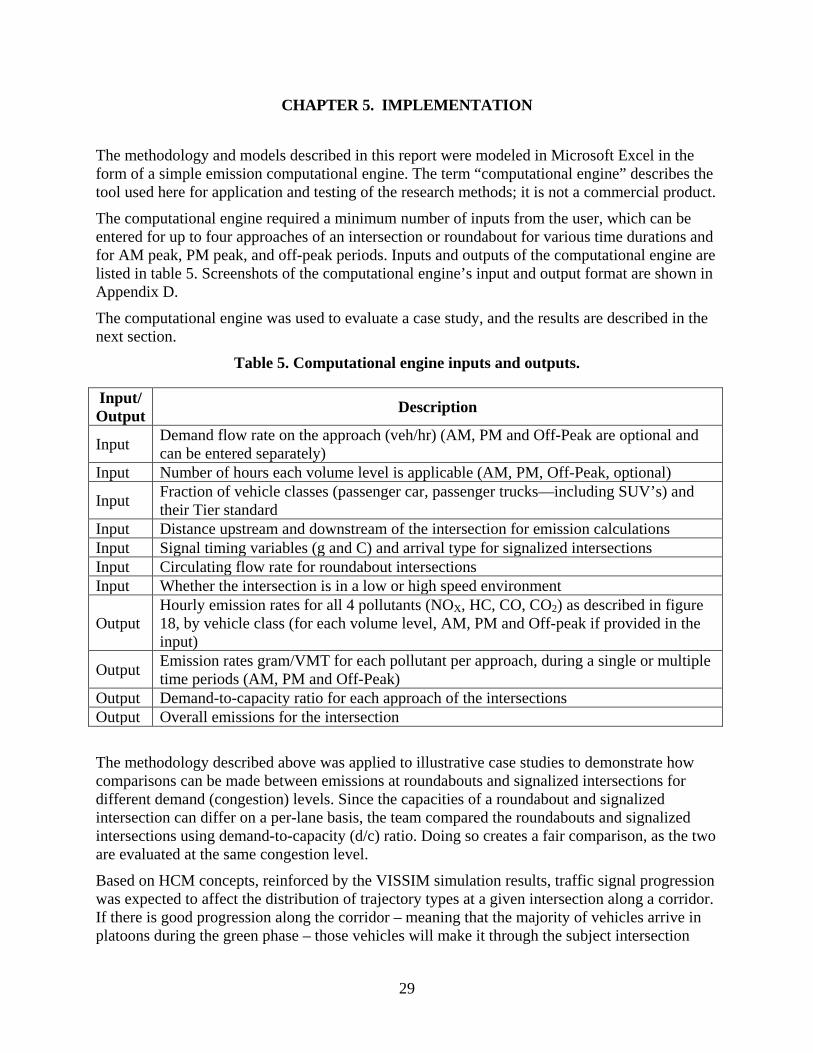
Table 5. Computational engine inputs and outputs. ................................................................ 29

Table 6. Computational engine inputs and outputs (from table 5). ....................................... 40

Table 7. Attributes of data collection routes. ........................................................................... 46

Table 8. Definition of VSP bins. ................................................................................................. 48

Table 9. List of the signalized intersections used for data collection. .................................... 51

Table 10. Coefficients of variables used for predicting the likelihood of a no-stop (Type A) speed profile at a signalized intersection approach (table 3). ................................................. 55

Table 11. Functions for predicting the proportion of a Type C profile at a signalized intersection approach (table 4). ................................................................................................. 55

1

CHAPTER 1. INTRODUCTION

Intersections are a major source of congestion on arterial streets. Signal optimization, alternative intersection designs, or alternative routes for traffic are among the techniques employed to mitigate intersection congestion. Congestion is deemed to be a significant source of vehicle emissions, because stop-and-go traffic and associated acceleration/deceleration patterns have been linked to increased emissions. Roundabouts can have operational and safety benefits over signalized intersections under certain circumstances. For example, the average vehicle delay can be significantly lower during off-peak periods for roundabouts compared to signalized intersections, and under peak traffic conditions, roundabouts can often match or even outperform traffic signals operationally. Due to the geometric and design characteristics of roundabouts, they can function as a traffic calming device, and they have been shown to provide substantial safety benefits over signalized intersections.

Roundabouts have also been characterized as a more environmentally-friendly form of intersection based on analyses comparing them to conventional signalized intersections.[1] In these analyses, simulation models determined that roundabouts experienced lower emissions due to less stop-and-go traffic patterns. However, the hypothesis that roundabouts experience lower vehicle emissions than signalized intersections has been largely untested. It has neither been field tested nor substantiated by extensive empirical research using vehicle emission patterns collected at roundabouts in the field.

The premise for this research is that the environmental performance of roundabouts is tied to their operational performance, with emission levels sensitive to traffic volume and congestion. An increase in traffic volume leads to an increase in stop-and-go traffic patterns, which in turn leads to an increase in emissions. The evaluation of the environmental performance of roundabouts therefore requires quantification of factors impacting their operation. The research also sought to create comparable methods for calculating emissions at roundabouts and at signalized intersections, so the results could be compared.

This research explored emission patterns of vehicles traversing roundabouts through empirical analysis of vehicle trajectories, and proposes a methodology to compare emissions generated at roundabouts to those generated at signalized intersections. The research incorporated emission factors for different classes of passenger cars and passenger trucks, any combination of which can be tested. Heavier classes of trucks were not included in this research, because calculating their emissions requires a different methodology. This research categorized roundabouts and signalized intersections into two bins based on approach speed: high speed (greater or equal to 56 km/h (35 mph)); and low speed (less than 56 km/h (35 mph)). Two predictive models were developed for the two speed groups.

BACKGROUND

A great deal of research has been performed regarding emissions generated at roundabouts. That research includes a large and diverse set of methods, and a similarly large and varied set of findings and conclusions. The lack of consensus in the research community, with respect to both methods and findings, justified this research. Before the literature is reviewed, some fundamental emission terms and variables must be defined to put the review in context.

2

First, five major factors impact vehicle fuel consumption and vehicle emissions on any roadway segment or intersection,[2] namely:

1. Driver behavior, especially in relation to vehicle acceleration/deceleration and driver aggressiveness.

2. Vehicle attributes, including vehicle age, weight, engine size, transmission, emissions prevention and control systems, and fuel type and condition.

3. Traffic conditions, characterized by the level of congestion and conflicting traffic. 4. Infrastructure design and control, including design speed, signal timing and grades. 5. Ambient conditions including temperature, humidity, and barometric pressure.

Second, a relationship and distinction between vehicle activity and vehicle emissions exists. Items 1, 3 and 4 are the principal items affecting vehicle dynamics, motion, or activity, and items 2 and 5 principally impact the resulting emission and fuel consumption rates. Any analysis of roundabout environmental effectiveness must account or control for those factors when comparing them to the competing types of control.

Most research on vehicle emissions at roundabouts recognizes that at the root of all vehicle activity is the individual vehicle trajectory, or the speed profile of the vehicle, as it traverses the segment or intersection of interest. Trajectories provide information on speed, acceleration and deceleration rates and idling times as a function of driver behavior, traffic conditions (congested vs. uncongested), roadway design, and control (roundabout vs. signal). In essence the trajectory captures all the effects listed in items 1, 3 and 4 above. In past research, trajectories have been measured directly in the field using Global Positioning System (GPS), Portable Emissions Measurement System (PEMS), or generated synthetically from macroscopic or microscopic simulation models.

Researchers must then link activity and trajectory to emissions, which can be done in many ways. In a simulation environment, trajectory estimates can be made for individual vehicles in the form of speed versus time at a second-by-second or lower resolution. Such trajectories can be used with modal emission models to estimate average emission rates or total emissions for a trajectory. The same computations can be performed for fuel usage. Vehicle operating modes, such as idle, acceleration, deceleration, and cruise can be determined given trajectory data. Moreover, operating modes can be estimated in terms of continuous ranges of engine load taking into account second-by-second speed and accelerations.[3]

For example, SIDRA uses a four-mode model of acceleration, deceleration, idle, and cruise to predict fuel and emissions. CORSIM uses look-up tables of instantaneous speed and acceleration rates to estimate emissions on a second-by-second basis. Other microscopic models such as VISSIM, Paramics, and AIMSUN provide their own emission estimation procedures embedded in the models, and are based on look-up tables for speeds and accelerations. Finally, in the PEMS emissions estimation approach, both vehicle activity and fuel and emissions are measured simultaneously, thus providing the firmest linkage between the two. The current MOVES model by the US Environmental Protection Agency[4] uses a series of emission factor models based on vehicle operating mode; modes are defined as unique combinations of Vehicle Specific Power (VSP) and speed. VSP is a function of instantaneous vehicle speed (v), vehicle acceleration (a) and road grade (r). VSP has consistently been found to be highly correlated with vehicle

3

emissions, and it is used in the MOVES model.[5,6] VSP is expressed using the equation in figure 1:

Figure 1. Equation. Vehicle specific power calculation.

The MOVES model can estimate emission rates and inventories at the project, county, and national scales. Emission factors can be estimated for selected vehicle source categories, model years, calendar years, ambient conditions, and driving schedules using a project-level analysis feature.

OBJECTIVE

The primary objective of this research was to develop a simplified methodology for estimating and comparing the pollutant emissions generated by vehicles passing through a roundabout and a signalized intersection, with the methodology based on actual, field-collected data. The methodology is macroscopic in nature, and uses inputs deemed readily available to analysts performing a planning-stage evaluation of roundabouts. A second objective of the research was to show how real-world data, including vehicle trajectories and other traffic characteristics such as demand, vehicle speed, approach capacity, signal timing, and the proportion of demand arrivals during the green phase (known as the “arrival type” in the HCM), affect the amount of pollutant emissions generated at signalized intersections and roundabouts. The research also attempted to identify variables and thresholds that may cause one type of intersection to have more pollutants than the other.

The methodology was developed and demonstrated using over 1,980 vehicle trajectories at roundabouts and signaled intersections at a one-second resolution. The VSP method was used as the key explanatory variable for emissions estimation.[5,7] Activity and emission models were developed using speed characteristics, demand, and signal timing. The basic outputs of the model are the average emission rates for four primary pollutants (including carbon monoxide (CO), hydrocarbon (HC), and mono-nitrogen oxides (NOX)), expressed in milligrams/vehicle, grams/hr, and grams/vehicle-mile-traveled (grams/VMT).

5

CHAPTER 2. LITERATURE REVIEW

Various research projects and simulation tools have attempted to compare emissions generated at roundabouts and signalized intersection under different traffic conditions. Hallmark et al.[8] found roundabouts had marginally better traffic flow within signalized corridors than stop-controlled and signalized intersections. The same authors then conducted a real-world, in-field assessment of vehicle emissions at a roundabouts compared to those at a signalized intersections.[9] The authors demonstrated that, when traffic was not congested, vehicles traversing roundabouts did not have lower emissions than those traversing signalized intersections in the same corridor. Other research[10] assessed the average speeds, delays, and travel times of six roundabouts along a rural corridor in South Africa and compared them to fixed-cycle traffic signals. The authors concluded that roundabouts had operational advantages over traffic signals, but also that roundabouts were inefficient in high-demand scenarios.

In contrast, U.S. researchers[11] concluded that the environmental benefits posed by converting a signalized intersection to a two-lane roundabout in an urban corridor were only meaningful at the intersection level and for right-turn movements from the minor street to the main street. They also found that, at the corridor-level, turning movements from the main street produced higher total emissions at the roundabout than at the signalized intersection, while turning movements from the minor street produced lower total emissions at the roundabout than at the signalized intersection. Other U.S. research[12] estimated that variability associated with driving behavior results in differences in vehicular emissions at a roundabout. Other studies have integrated simulated vehicle dynamic data and microscopic modeling to estimate vehicle emissions at roundabouts.[13,14,15] In these studies, the findings were inconclusive regarding the benefits from roundabouts concerning emissions reductions.

The effect of speed and acceleration on arterials on fuel consumption is complex. High fuel consumption rates on arterials are typically associated with driving in congested traffic, characterized by higher speed fluctuations and frequent stops at intersections, leading to frequent accelerations.[16] The accelerations lead to high fuel use rates compared to idling or deceleration.[16] However, low traffic and continuous progression along streets dis not guarantee the lowest fuel consumption and emissions rates. The authors[16] further suggested that the best flow of traffic on arterial streets in terms of fuel consumption and emissions is the one with the fewest stops, shortest delays, and moderate speeds maintained throughout the commute.

Other research on arterials found that, to investigate emissions on existing arterial roads using micro-simulation models, and to study the effects of improvements to traffic flow, the simulated traffic on arterials must accurately represent that in the real world. SIDRA is a software tool enabling evaluation of vehicle emissions, especially at roundabouts and other forms of intersections.[17] SIDRA defines drive cycles for the simulated traffic based on initial and final speed for each element of a driving maneuver. The drive cycle is used to calculate delays, queues, number of stops, and acceleration and decelerations. The information is then used to calculate the fuel consumption and emission rates based on a set of set of equations.

Roundabouts and signalized intersections are hypothesized to have different localized effects on vehicle second-by-second (1 Hz) speed trajectories.[11] Research has documented that vehicle emissions depend on this second-by-second resolution engine load, and has further demonstrated

6

that this second-by-second engine load can be closely estimated using VSP.[6] VSP is based on second-by-second road grade, and the speed and acceleration profiles of the vehicle. Vehicle fuel use and the emission rates of tailpipe exhaust pollutants, including CO, HC, and NOX, are highly sensitive to the underlying VSP distribution.[5,7] VSP is the underlying conceptual basis for the U.S. Environmental Protection Agency’s MOVES vehicle emission factor model.[5]

A recent study investigated the amount of error in emissions estimates using VSP distributions of vehicle activity data from VISSIM and the sensitivity of VSP distributions to modeling parameters.[18] It was observed that second-by-second empirical vehicle activity data and simulated vehicle activity data from a calibrated and validated VISSIM model did not yield the same VSP distributions and the results needed to be calibrated using GPS data.

Relevant research studies on emissions at roundabouts and other intersections are listed in table 1. They are summarized in terms of activity measurements, estimated emissions and principal findings. No one standard method or approach currently analyzes the environmental impact of intersection control type, although certain approaches are more widely used than others.

Table 1. Survey of emissions studies at roundabouts and other intersection controls.

Cited Research Study

Vehicle Activity Source

Fuel & Emissions Model Source

Roundabout Environmentally

Effective? Ahn et al. (2009)[13] VISSIM VT-Micro/CMEM Negative when congested

Chamberlain et al. (2011)[14] Own Micro-Model CMEM/MOVES Negative impact

Coelho et al. (2006)[1] Synthetic Profiles VSP Congestion-dependent

impact Hallmark et al. (2011)[9] PEMS PEMS Inconclusive-low traffic

Mandavilli et al. (2008)[15] SIDRA SIDRA Positive impact

It is clear from the literature review that the findings are mixed, and to some extent dependent on the approach used to estimate activity and emissions. Analysis tools, whether macroscopic or microscopic, make assumptions regarding driver behavior and vehicle motion, none of which appears to have been thoroughly vetted against actual recorded vehicle data at roundabouts. This is a critical component of our approach to emissions modeling: we measured vehicle performance in the field. The same applies to the emission factor models. PEMS activity and emissions data at roundabouts have been collected on a limited basis involving very few drivers and limited traffic congestion levels. That data is not enough to enable the analyst to reach meaningful statistical conclusions regarding the effect of intersection type on emissions. In order to disentangle the confounding effects of driver behavior and congestion levels from the type of intersection control, more controlled methods are needed.

7

CHAPTER 3. METHODOLOGY

The literature review identified a limited number of studies that have inferred that vehicle emissions at roundabouts were less than that at signalized intersections. However, there is no simplified methodology allowing an analyst to readily compare the emissions at roundabouts and signalized intersections over a range of traffic conditions and in a deterministic analysis framework. Further, most prior research used models were not calibrated using real world, in-field trajectory data collected in the United States.

To evaluate the differences in emissions between roundabouts and signalized intersections, this project developed a method taking into account speed trajectories and their effect on emissions over a period of vehicle operation of approximately one minute. Although traffic simulation models can simulate second-by-second speed trajectories, they are typically calibrated using macroscopic parameters, and the accuracy of the trajectories themselves has been shown to not match real-world driving behavior, particularly on urban arterials.[11] Therefore, this research developed a method based on measured real-world trajectories. The data used to develop the method could also be used to evaluate simulated trajectories from traffic simulation models.

This research uses the concept of VSP as the basis for estimating emissions associated with a speed trajectory.[5,7] The methodology relies on a combination of PEMS and GPS field studies to characterize both vehicle activity and fuel and emissions at a second-by-second level. An illustration of the PEMS system used in this project is depicted in figure 2 and figure 3.

. To account for varying driver acceleration and deceleration profiles, the team used existing and new activity and emissions data from multiple drivers to capture the mean and variance of activities across drivers. To account for the impact of congestion, the team sorted the activity data into congestion-dependent bins as documented in research.[1]

8

Figure 2. Photo. Illustration of PEMS tailpipe emissions measurement (for additional

details on PEMS see [2]).

Figure 3. Photo. Illustration of PEMS computer recording unit (for additional details on

PEMS see [2]).

The methodology used in this research is based on two categories of models. The first category is Activity Models. There are a total of six models in this category, with three speed-profile models for roundabouts and three for signalized intersections. The three models within each intersection type differed in terms of the frequency of trajectory types A (those experiencing no stops), B (those experiencing a single stop at the stop or yield line) and C (multiple stops in the queue and at the stop or yield line). The trajectory types are a function of the approach or conflicting demand volume. The data for developing the three activity models for roundabouts were collected from observing overhead videos of roundabouts and classifying each vehicle arrival into one of the three trajectory categories. The data for signalized intersections included real-world trajectories of vehicles approaching signalized intersections; however, the models for estimating the proportion of Type A, B, and C trajectories at signals, however, were estimated from a series of VISSIM simulation models. The latter approach was needed, because a multitude of factors impact the probability of no stops, single stops, or multiple stops, including

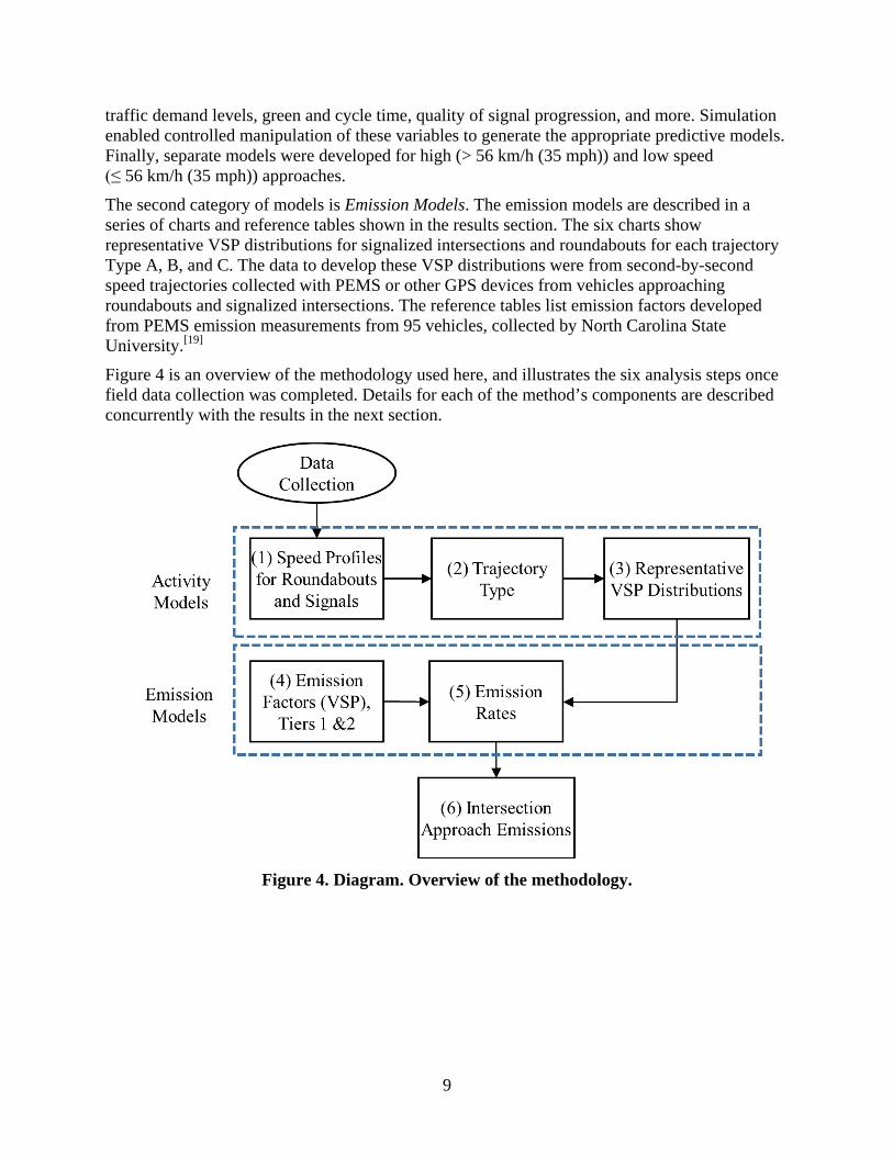
9

traffic demand levels, green and cycle time, quality of signal progression, and more. Simulation enabled controlled manipulation of these variables to generate the appropriate predictive models. Finally, separate models were developed for high (> 56 km/h (35 mph)) and low speed (≤ 56 km/h (35 mph)) approaches.

The second category of models is Emission Models. The emission models are described in a series of charts and reference tables shown in the results section. The six charts show representative VSP distributions for signalized intersections and roundabouts for each trajectory Type A, B, and C. The data to develop these VSP distributions were from second-by-second speed trajectories collected with PEMS or other GPS devices from vehicles approaching roundabouts and signalized intersections. The reference tables list emission factors developed from PEMS emission measurements from 95 vehicles, collected by North Carolina State University.[19]

Figure 4 is an overview of the methodology used here, and illustrates the six analysis steps once field data collection was completed. Details for each of the method’s components are described concurrently with the results in the next section.

Figure 4. Diagram. Overview of the methodology.

11

CHAPTER 4. RESULTS

This section presents the results of the emissions estimation methodology. Results are presented in the sequence of the overall methodology, as shown in the flowchart in figure 4. The methodology starts with the activity models and moves on to the emissions models.

ACTIVITY MODELS

The activity model component of the analysis methodology consisted of (1) the speed profiles for roundabouts and signalized intersections, and (2) the estimation of the frequency for Trajectory Types A, B, and C. The two components are discussed in order below.

Speed Profiles

Based on field measurements from available research on emissions,[1,20] there are three general classifications for speed trajectories of a vehicle approaching an intersection. These classifications are distinguished based on changes in speed, duration, and number of stop-and-go cycles at the intersection, and changes in the acceleration and deceleration profiles. An individual vehicle trajectory through a roundabout or a signalized intersection can take on a variety of shapes in terms of speed versus time, as shown in figure 5. The three speed profiles were:

A. No stop through the intersection. B. Single stop at the intersection entry approach, normally at the front of the queue. C. Multiple stops as the vehicle joins the back of the queue at the intersection approach.

It is hypothesized that vehicles experiencing each of these speed profiles generate different levels of emissions. Type A was expected to generate the least amount of emissions because it has the least amount of acceleration and deceleration. On the other extreme, Type C was expected to generate the highest amount of emission because it has the most acceleration and deceleration cycles. The three speed profiles are illustrated in figure 5.

12

Figure 5. Graph. Illustration of the three types of trajectories (A: no-stop, B: one-stop, and

C: multiple-stops) for a roundabout and signalized intersection approach.

In figure 5, the green (solid) line shows the three speed trajectory classes for a roundabout approach. Variations shown with the orange dashed lines denote speeds at signals that are hypothesized to be different than those at roundabouts. For a Type A trajectory, speeds through the roundabout are lower due to the curvature and geometry of the circulatory roadway compared to those through intersections, where vehicles going straight through might not have to slow down. For Type B and C trajectories, vehicles come to a complete stop, so vehicle acceleration/deceleration is expected to be more rapid at signals than at roundabouts, again because the roadway curvature at roundabouts constrains the vehicle trajectories.

The proportions of vehicles experiencing these three types of speed trajectories is expected to be sensitive to the level of traffic demand on the intersection approach, and at signalized intersections, the signal timing. The team constructed the emissions estimation models based on VSP as a function of these three speed trajectory types. The frequency models estimate the probability that an approaching vehicle will experience no-stops, one-stop, or multiple-stops. The corresponding VSP distribution models for each of the speed trajectory types was then invoked. Separate VSP distribution models were developed for low-speed intersection approaches (free-flow speed less than or equal to 56 km/h (35 mph)) and high-speed intersection approaches (free-flow speed more than 56 km/h (35 mph)) at both signalized intersections and roundabouts. The 56 km/h (35 mph) threshold was chosen based on the speed data available from study locations, representing a natural break between low speed and high-speed approaches under study. A detailed explanation of each of these models follows.

13

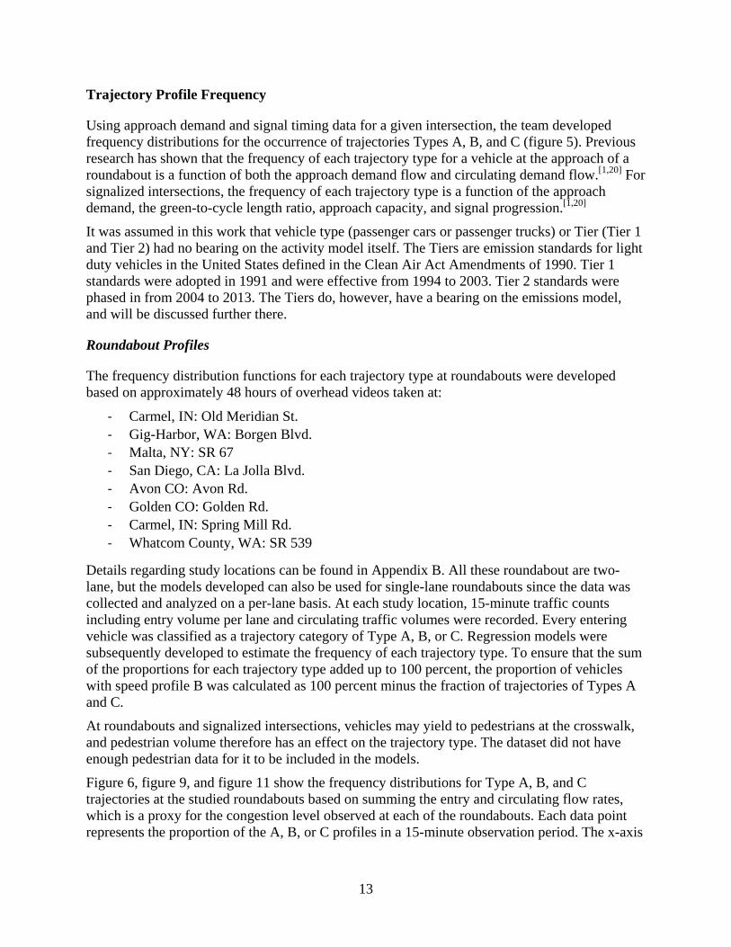
Trajectory Profile Frequency

Using approach demand and signal timing data for a given intersection, the team developed frequency distributions for the occurrence of trajectories Types A, B, and C (figure 5). Previous research has shown that the frequency of each trajectory type for a vehicle at the approach of a roundabout is a function of both the approach demand flow and circulating demand flow.[1,20] For signalized intersections, the frequency of each trajectory type is a function of the approach demand, the green-to-cycle length ratio, approach capacity, and signal progression.[1,20]

It was assumed in this work that vehicle type (passenger cars or passenger trucks) or Tier (Tier 1 and Tier 2) had no bearing on the activity model itself. The Tiers are emission standards for light duty vehicles in the United States defined in the Clean Air Act Amendments of 1990. Tier 1 standards were adopted in 1991 and were effective from 1994 to 2003. Tier 2 standards were phased in from 2004 to 2013. The Tiers do, however, have a bearing on the emissions model, and will be discussed further there.

Roundabout Profiles

The frequency distribution functions for each trajectory type at roundabouts were developed based on approximately 48 hours of overhead videos taken at:

- Carmel, IN: Old Meridian St. - Gig-Harbor, WA: Borgen Blvd. - Malta, NY: SR 67 - San Diego, CA: La Jolla Blvd. - Avon CO: Avon Rd. - Golden CO: Golden Rd. - Carmel, IN: Spring Mill Rd. - Whatcom County, WA: SR 539

Details regarding study locations can be found in Appendix B. All these roundabout are two-lane, but the models developed can also be used for single-lane roundabouts since the data was collected and analyzed on a per-lane basis. At each study location, 15-minute traffic counts including entry volume per lane and circulating traffic volumes were recorded. Every entering vehicle was classified as a trajectory category of Type A, B, or C. Regression models were subsequently developed to estimate the frequency of each trajectory type. To ensure that the sum of the proportions for each trajectory type added up to 100 percent, the proportion of vehicles with speed profile B was calculated as 100 percent minus the fraction of trajectories of Types A and C.

At roundabouts and signalized intersections, vehicles may yield to pedestrians at the crosswalk, and pedestrian volume therefore has an effect on the trajectory type. The dataset did not have enough pedestrian data for it to be included in the models.

Figure 6, figure 9, and figure 11 show the frequency distributions for Type A, B, and C trajectories at the studied roundabouts based on summing the entry and circulating flow rates, which is a proxy for the congestion level observed at each of the roundabouts. Each data point represents the proportion of the A, B, or C profiles in a 15-minute observation period. The x-axis

14

shows the 15-minute flow rate in vehicles per hour during the observation periods. Approximately 190 15-minute observations were used to create the dataset. The user can adjust the A, B or C profile distributions as available from local data. The observed flow rates were between 200 to 1700 vph.

Figure 6 shows the proportion of vehicles entering the roundabout without stopping (Type A). The data collected at the roundabouts shows that this proportion can be estimated using a cumulative normal distribution with a mean value of 720 and a standard deviation of 340. This means that if the combined approach and conflicting flow rate at the roundabout is equal to 720 vph, 50 percent of the vehicles would not stop. The R-squared value for the model is 0.51.

Figure 6. Graph. Prediction model for proportion of no-stop trajectory (Type A).

The proportion of the number of stops in trajectory Type A is calculated from a normally-distributed cumulative distribution function (CDF) with parameters shown in figure 7:

Figure 7. Equation. Proportion of Type A trajectories (no stops).

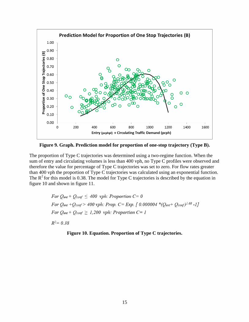
The proportion of Type B trajectories is shown in figure 9. As mentioned before, to ensure that the sum of the proportion of each trajectory type adds up to 100 percent, the proportion of vehicles with Type B trajectories was calculated as equal to 100 percent minus the percentage of Types A and C trajectories. Thus, it is calculated as shown in figure 8:

Figure 8. Equation. Proportion of Type B trajectories.

15

Figure 9. Graph. Prediction model for proportion of one-stop trajectory (Type B).

The proportion of Type C trajectories was determined using a two-regime function. When the sum of entry and circulating volumes is less than 400 vph, no Type C profiles were observed and therefore the value for percentage of Type C trajectories was set to zero. For flow rates greater than 400 vph the proportion of Type C trajectories was calculated using an exponential function. The R2 for this model is 0.38. The model for Type C trajectories is described by the equation in figure 10 and shown in figure 11.

Figure 10. Equation. Proportion of Type C trajectories.

16

Figure 11. Graph. Prediction model for proportion of multiple-stop trajectory (Type C).

Signalized Intersections

At signalized intersections, the modeling approach differed from that of the strictly empirical roundabout models. It was hypothesized that the likelihood of experiencing one or multiple stops at a signalized intersection was correlated to the signal timing on the approach, the level of signal progression (or the proportion of vehicles that arrive during the green phase), and the demand-to-capacity ratio (d/c) for the approach. Given the more predictable and cyclical nature of traffic patterns at signals compared to roundabouts, the Highway Capacity Manual[21] approach for characterizing signal progression was used to help develop the functional forms for frequency models for Type A, B, and C trajectories at signalized intersections. Actual trajectory A, B, and C frequencies were obtained from a simple simulation experiment designed in the VISSIM microsimulation model[22]. The experiment varied the approach demand, g/C ratio (effective green to cycle length ratio), d/c ratio (demand to capacity ratio), and modeled all HCM arrival types by changing the signal offset at two signalized intersections.

The HCM defines six arrival types to describe signal progression quality, with one being very poor progression and six being exceptional progression, as listed in table 2. It is known that progression quality, or arrival type, affects the speed trajectory of the vehicles and the number of stops vehicles experience as they go through a signalized intersection.

17

Table 2. Progression quality and arrival type (Source [21]).

Arrival Type

Progression quality

Platoon Ratio (Rp)

Conditions Under Which Arrival Type Is Likely to Occur

1 Very poor 0.33 Coordinated operation on a two-way street where the subject direction does not receive good progression

2 Unfavorable 0.67 A less extreme version of Arrival Type 1 3 Random

Arrivals 1.00 Isolated signals or widely spaced coordinated signals

4 Favorable 1.33 Coordinated operation on a two-way street where the subject direction receives good progression

5 Highly Favorable

1.67 Coordinated operation on a two-way street where the subject direction receives good progression

6 Exceptional 2.00 Coordinated operation on a one way street in dense networks and central business districts

For the VISSIM simulation two sets of eight models were developed. The design of the VISSIM network is a simple two-lane (two lanes per approach) link network with two pre-timed signals located at a specific distance of 457 m (1500 ft) from each other on this link. The first set of eight models simulated a high speed environment with an average free-flow speed of 72 km/h (45 mph), and the second set of eight models simulated an environment with an average free-flow speed of 56 km/h (35 mph). Since the speeds follow a normal distribution in VISSIM with standard deviation of 11 km/h (7 mph), a range of vehicle speeds were captured through the simulation. The signals in the models have a cycle length of 120 s.

Each of the eight models in each represents a specific g/C ratio, which is achieved by varying the effective green (g) values (30 s, 40 s, 50 s, 60 s, 70 s, 80 s, and 90 s) while keeping the cycle length constant at 120 s. The signal offset (quantity describing relative start time of coordinated phases for adjacent signals) was set to simulate three arrival patterns: (1) poor progression, (2) random arrival, and (3) good progression.

The traffic volume during the simulation period was varied for each of the models to cover a d/c ratio range from 0.1 to approximately 1.4. All scenarios had 48 simulation models, and each model was run 10 times, resulting in 480 simulation runs, each for a period of 1 h. After the simulation runs were complete, a macro was developed to process each modeled vehicle trajectory and to calculate the fraction of A, B, and C trajectory types for the simulation period. The data was used to develop the models in table 3. Additional details and sample output from the simulation are included in Appendix C.

The combination of simulation and HCM-based arrival type models showed that the proportion of vehicles with Type A speed trajectories depended on the green-to-cycle length ratio (g/C), demand-to-capacity ratio (d/c), and the platoon ratio (Rp). The platoon ratio depended on the level of signal progression, which in turn was estimated from HCM arrival types and the proportion of vehicles arriving during green. The model coefficients were also sensitive to the quality of signal progression along the corridor. The functional form of the estimated relative frequency of A profiles at signals is shown in the equation in figure 12.

18

Figure 12. Equation. Proportion of trajectory Type A, modified.

Where:

b0 = intercept value which is a function of arrival type (or HCM platoon ratio)

b1 = coefficient for d/c ratio

d/c = demand to capacity ratio on the signalized approach; capacity per lane is = S g/C, where S is the lane saturation flow rate

b2 = power coefficient for the d/c ratio

Rp = platoon ratio which varies from 0.33 to 2 depending on arrival type (arrival Type 1: very poor to 6: exceptionally favorable. Values can be found in table 3

g/C = approach (through) effective green to cycle length ratio

Table 3 lists the associated coefficients for each HCM arrival type estimated from the simulation experiments, with higher arrival types referring to generally better progression quality on an arterial street.[21]

Table 3. Coefficients of variables used for predicting the likelihood of no-stop (Type A) speed profile at a signalized intersection approach.

Arrival Type

Platoon Ratio, Rp

b0 b1 b2

1 0.33 Min[1,Rp(g/c)] -0.0195+0.580*g/C 3 2 0.67 Min[1,Rp(g/c)] -0.0195+0.580*g/C 3 3 1 Min[1,Rp(g/c)] -0.0195+0.580*g/C 3 4 1.33 Min[1,Rp(g/c)] -0.9809(g/C)2+1.2748(g/C)-0.0149 5(Rp g/C) 5 1.67 Min[1,Rp(g/c)] -1.7314(g/C)2+1.9424(g/C)-0.0852 4(Rp g/C) 6 2 Min[1,Rp(g/c)] -2.2578(g/C)2+2.1815(g/C)-0.0487 4(Rp g/C)

As an illustrative example, let the HCM arrival type be 2, g/C be 0.4, and d/c be 0.80. The relative Type A trajectory frequency then is calculated using the equation in figure 13.

Figure 13. Equation. Example of Type A trajectory calculation.

This result suggests that 16 percent of the approaching vehicles would not stop on this approach.

The proportion of vehicle experiencing Type C trajectories is formulated as a function of signal progression (HCM arrival types) and demand-to-capacity ratio. Similar to roundabouts, the proportion of Type B trajectories is calculated as the difference between 100 percent and the proportion of A plus C trajectories. The proposed models for estimating the relative frequency of speed trajectory Type C are shown in table 4.

19

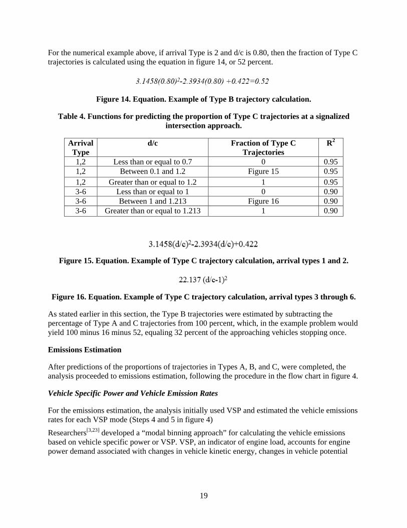
For the numerical example above, if arrival Type is 2 and d/c is 0.80, then the fraction of Type C trajectories is calculated using the equation in figure 14, or 52 percent.

Figure 14. Equation. Example of Type B trajectory calculation.

Table 4. Functions for predicting the proportion of Type C trajectories at a signalized intersection approach.

Arrival Type

d/c Fraction of Type C Trajectories

R2

1,2 Less than or equal to 0.7 0 0.95 1,2 Between 0.1 and 1.2 Figure 15 0.95 1,2 Greater than or equal to 1.2 1 0.95 3-6 Less than or equal to 1 0 0.90 3-6 Between 1 and 1.213 Figure 16 0.90 3-6 Greater than or equal to 1.213 1 0.90

Figure 15. Equation. Example of Type C trajectory calculation, arrival types 1 and 2.

Figure 16. Equation. Example of Type C trajectory calculation, arrival types 3 through 6.

As stated earlier in this section, the Type B trajectories were estimated by subtracting the percentage of Type A and C trajectories from 100 percent, which, in the example problem would yield 100 minus 16 minus 52, equaling 32 percent of the approaching vehicles stopping once.

Emissions Estimation

After predictions of the proportions of trajectories in Types A, B, and C, were completed, the analysis proceeded to emissions estimation, following the procedure in the flow chart in figure 4.

Vehicle Specific Power and Vehicle Emission Rates

For the emissions estimation, the analysis initially used VSP and estimated the vehicle emissions rates for each VSP mode (Steps 4 and 5 in figure 4)

Researchers[3,23] developed a “modal binning approach” for calculating the vehicle emissions based on vehicle specific power or VSP. VSP, an indicator of engine load, accounts for engine power demand associated with changes in vehicle kinetic energy, changes in vehicle potential

20

energy (e.g., hill climbing), rolling resistance, and aerodynamic drag,[7] and is calculated using the equation in figure 17.

Figure 17. Equation. Vehicle specific power calculation (from figure 1).

Where:

VSP = Vehicle specific power at 1 Hz resolution (kW/ton)

v = Speed at 1 Hz resolution (m/s)

a = Acceleration at 1 Hz resolution (m/s2)

grade = The terrain gradient for change in elevation versus distance (ratio)

VSP values estimated at second-by-second resolution (1 Hz) are categorized into 14 modes and are shown in figure 18.[3,23] VSP modes 1 and 2 are for negative VSP values associated with deceleration or travel on negative (down-sloping) road grades. VSP mode 3 is for idle. VSP modes 4 to 14 are for ranges of increasing positive VSP, which can represent acceleration, steady-speed cruising at various speeds, or climbing hills with positive road grade. Average VSP modal emission rates were estimated for each vehicle. These modal rates were weighted by the amount of time spent in each VSP mode for a given speed trajectory to estimate trajectory-average rates.

21

T1 PC (n=24); T2 PC (n=39) Tier 1 Passenger Cars, Average Emission Rates Tier 2 Passenger Cars, Average Emission RatesVSP Mode VSP Range* NOx_mg/s HC_mg/s CO_mg/s CO2_g/s NOx_mg/s HC_mg/s CO_mg/s CO2_g/s

1 VSP<-2 0.8 0.2 3.9 1.2 0.6 0.3 1.4 1.12 -2≤VSP<0 1.0 0.3 4.8 1.4 0.6 0.2 1.6 1.33 0≤VSP<1 0.4 0.2 3.3 1.0 0.2 0.2 1.3 0.9

rs 4 1≤VSP<4 1.9 0.5 8.5 2.4 1.2 0.4 2.7 2.2ar C

5 4≤VSP<7 2.8 0.6 11.3 3.3 1.8 0.5 3.7 3.06 7≤VSP<10e 3.8 0.8 13.8 4.1 2.3 0.6 5.0 3.8

g 7 10≤VSP<13 4.9 0.9 17.0 4.9 2.5 0.7 6.8 4.5nss

e 8 13≤VSP<16 5.9 1.0 19.6 5.5 2.6 0.8 7.8 5.19 16≤VSP<19 7.1 1.1 24.7 6.1 2.7 0.9 10.3 5.7aP 10 19≤VSP<23 7.8 1.2 28.6 6.5 2.8 1.0 12.4 6.211 23≤VSP<28 9.1 1.3 36.5 6.9 3.4 1.1 16.7 6.712 28≤VSP<33 10.7 1.4 46.0 7.5 4.0 1.1 27.3 7.413 33≤VSP<39 12.7 1.6 70.9 8.0 4.7 1.3 34.9 8.214 39≤VSP 11.7 1.9 187.7 8.7 6.5 1.4 69.5 9.2

T1 PT (n=10), and T2 PT (n=22) Tier 1 Passenger Trucks, Average Emission Rates Tier 2 Passenger Trucks, Average Emission RatesVSP Mode VSP Range* NOx_mg/s HC_mg/s CO_mg/s CO2_g/s NOx_mg/s HC_mg/s CO_mg/s CO2_g/s

1 VSP<-2 0.8 0.5 7.4 1.8 0.2 0.4 3.8 1.92 -2≤VSP<0 0.9 0.5 7.2 2.1 0.2 0.4 4.0 2.3

s 3 0≤VSP<1 0.3 0.4 2.8 1.4 0.0 0.2 2.1 1.4kc 4 1≤VSP<4 1.8 0.8 12.8 3.4 0.3 0.6 6.6 3.5

ru 5 4≤VSP<7 2.9 1.0 18.1 4.6 0.4 0.8 9.8 4.8

r T 6 7≤VSP<10 3.9 1.3 24.8 5.7 0.6 1.1 12.0 6.0

e 7 10≤VSP<13 5.2 1.5 26.8 6.6 0.7 1.2 14.9 7.0gn 8 13≤VSP<16 6.3 1.7 29.1 7.5 0.8 1.3 16.9 8.0

sse 9 16≤VSP<19 8.1 2.0 35.1 8.2 1.0 1.5 19.4 9.0

a 10 19≤VSP<23 8.7 2.2 40.2 8.8 1.2 1.7 27.6 9.8

P 11 23≤VSP<28 11.0 2.4 53.6 9.6 1.5 1.9 28.5 10.712 28≤VSP<33 13.9 2.6 78.1 10.7 1.9 2.0 37.3 11.813 33≤VSP<39 14.7 2.8 97.9 12.0 2.4 2.3 56.8 13.214 39≤VSP 20.8 3.1 171.6 13.0 3.2 2.8 149.3 15.7

* The VSP Ranges are the ranges of VSP values in KW/ton for each VSP mode

Figure 18. Image. Table of average emission rates by vehicle specific power (VSP) mode for Tier 1 and Tier 2 passenger cars and passenger trucks (Source: [23]).

Figure 18 lists a summary of emission data collected from 95 vehicles.[23] Emission data for each of the 95 vehicles were collected using three key instruments: (1) the OEM-2100 “Axion System” PEMS manufactured by Clean Air Technologies International, Inc.; (2) a Garmin GPS receiver with barometric altimeter; and (3) a “scantool” data logger for the on-board diagnostic (OBD) link of the vehicle electronic control unit (ECU)[3]. The PEMS measures the tailpipe exhaust concentrations of carbon dioxide (CO2), carbon monoxide (CO), hydrocarbons (HC), nitric oxide (NOX), and oxygen (O2). The data went through a detailed and robust quality-control and quality-assurance process before being used for the analysis.

The OBD scantool was used to record vehicle and engine data including vehicle speed, mass fuel flow (MFF), engine revolutions per minute (RPM), and others. Road grade was quantified based on data from global position system (GPS) receivers with barometric altimeters.[2] Data analysis included: (1) converting OBD data to a second-by-second basis[7]; (2) synchronizing second-by-

22

second data from multiple instruments into one database[2]; (3) quality assurance (QA); and (4) modal analysis of the data.[2]

From 2008 to the present, data have been collected for passenger cars (PCs) and passenger trucks (PTs) in the Research Triangle Park, NC area, including parts of Raleigh, Cary, Durham, Apex and Morrisville. Data for vehicle activity on multiple road functional classes (e.g., feeder/collector streets, minor arterials, major arterials, freeways, and ramps) and a wide range of speeds and accelerations[2,3] were collected. More details on the data collection routes and map of the routes can be found in Appendix B.

Passenger cars were defined as light duty vehicles intended for the carriage of passengers.[4] Passenger trucks were defined as minivans, pick-ups, sport utility vehicles (SUVs), and other two-axle, four-tire trucks used primarily for personal transportation and with gross vehicle weight less than 14,000 lbs.[4] Data were collected for 1997 to 2013 model years. For each vehicle, there were typically over 12,000 seconds of valid, quality-assured data. Heavier classes of trucks require a separate methodology for emissions calculation and were not included here.

The vehicle sample includes vehicles subject to different emission standards for light duty vehicles in the U.S., Tier 1 and Tier 2, defined according to the Clean Air Act Amendments of 1990. The measured vehicles of model years 1997 to 2003 were certified under Tier 1 (T1) exhaust emission standards, and those for model years 2004 to 2013 were certified under the more stringent Tier 2 (T2) standards.[24,25] Tier 2 standards were phased in from 2004 to 2013. PCs and PTs are subject to the same standards. Fleet average VSP modal rates were estimated for each of four vehicle groups: T1 PC (n=24); T2 PC (n=39); T1 PT (n=10), and T2 PT (n=22). The mean values for pollutants NOX, HC, CO2 and CO for VSP modes (emission factors) are shown in figure 18.

Typically, the modal emission rates are lowest for VSP Mode 3 and increase monotonically from Mode 3 to 14. The trends differ by pollutant; for example, the ratio of mean emission rate for Mode 14 versus Mode 13 is much higher for CO than for other pollutants. Therefore, differences in speed trajectories will affect emission rates among pollutants differently.

Generating Representative VSP Distributions

Building on the VSP modes and emissions rates described above, representative VSP distributions were developed for both roundabouts and signalized intersections (Step 3 in figure 4). Over 1,980 speed trajectories at a second-by-second resolution were collected from 42 signalized intersections in North Carolina and 24 roundabouts in six states across the country (Appendix B). The speeds were collected with a GPS unit from vehicles driving through the two intersection types at the speed typical for that roundabout or signalized intersection.

The magnitude and frequency of changes in speed are the primary factors affecting emissions. The research hypothesized that slowing down or coming to a full stop to enter an intersection or roundabout from higher approach speeds requires higher deceleration rates than doing so from lower approach speeds. It would also require higher acceleration rates after passing through the intersection or roundabout, and emission rates were also expected to be higher. The distinction is particularly important for roundabouts, since vehicles have to slow down to negotiate the curves as they enter the roundabout. Thus, for each intersection, vehicle speeds were extracted from mid-block upstream of the intersection to mid-block downstream of the intersection. Based on

23

the speed data available from all the intersections, two types of models were generated for low-speed and high-speed intersection approaches. The 56 km/h (35 mph) threshold was chosen based on the speed data available from study locations, with the given threshold showing a natural break in the collected data.

For each speed trajectory analyzed, the VSP was estimated for every second of the trajectory, and the emission rate for the corresponding VSP was selected. The process was repeated for the 1,980 available speed profiles. The overall distribution of time spent in each VSP mode was estimated for each type of intersection (roundabout, signalized intersection), speed range (low, high), and trajectory (Type A, B, and C).

Figure 19, figure 20, and figure 21 show the VSP distribution, or the percent of time spent in each VSP mode, for low-speed roundabouts and signalized intersections for each trajectory type. Figure 22, figure 23, and figure 24 show the same results, but for high-speed roundabouts and signalized intersections. The VSP distributions shown in those six figures were used to calculate pollutant emissions as follows:

1- Obtain the amount of gram (or milligram) per second for each pollutant is known for each VSP mode rom the emission factors in figure 18.

2- Calculate the travel time through the intersection for a given input travel distance based on average speeds for each trajectory (Type A, B C).

3- Estimate how many seconds of travel time through the intersection is spent in each VSP mode, based on the VSP distribution (see figure 19 through) defined for a given trajectory (Type A, B and C) and for either a signalized intersection or a roundabout.

4- Calculate the total grams of pollutant emissions for the given distance (segment length). 5- Estimate what proportion of vehicles experience each of the three types of profiles, based on

the frequency functions. 6- Prorate the total emission rates based on proportion of A, B and C speed profiles in the

approach traffic flow.

Figure 19. Chart. Percent time spent in VSP modes at low speed approaches for trajectory

Type A.

24

Figure 20. Chart. Percent time spent in VSP modes at low speed approaches for trajectory

Type B.

Figure 21. Chart. Percent time spent in VSP modes at low speed approaches for trajectory

Type C.

25

Figure 22. Chart. Percent time spent in VSP modes at high speed approaches for trajectory

Type A.

Figure 23. Chart. Percent time spent in VSP modes at high speed approaches for trajectory

Type B.

26

Figure 24. Chart. Percent time spent in VSP modes at high speed approaches for trajectory

Type C.

Intersection Approach Emission Estimation Method Using VSP

In the final step, the emission estimates were aggregated by intersection approach. Since VSP is a function of instantaneous speed and acceleration rates, the three trajectory types had distinctive effects on the distribution of time spent in each VSP mode and subsequently on the trajectory average emission rate. Therefore, to calculate hourly (or on any other time scale) emissions generated by vehicles approaching the intersection, the distribution of the three types of trajectories was taken into account, as shown in the equation in figure 25.

Figure 25. Equation. Hourly emission by vehicles approaching an intersection.

Where:

PI = Proportion of vehicles in the traffic stream in each speed profile i = A, B and C;

Qin = Entry demand flow rate (vph);

Ei = Emission associated with each speed profile, per vehicle (gms or mgms)

The total hourly emission was estimated from the sum of emissions generated by each speed profile (Ei), multiplied by the proportion of approach vehicles in that speed profile (Pi), and the hourly entry flow of the approach (Qin). The emissions can also be estimated for other timescales or longer time durations by adjusting for entry flow and number of hours. In order to estimate the emission for each speed profile (Ei), second-by-second emission rates for the vehicle with that speed profile were calculated from the VSP equation in figure 1/figure 17.

Therefore Ei is shown in figure 26.

27

Figure 26. Equation. Total emission for each speed profile.

Where:

EFn = Emission factor (g/s) assigned to the nth second of the speed profile based on the instantaneous VSP mode. The value of EFn for each pollutant is based on the VSP calculated for instantaneous speed (see figure 18).

Ni = Number of seconds in profile i; Ei = Total emissions associated with each of the three profiles (i.e., i = Type A, B or C).

In order to calculate Ei complete second-by-second speeds for each speed profile were needed.

29

CHAPTER 5. IMPLEMENTATION

The methodology and models described in this report were modeled in Microsoft Excel in the form of a simple emission computational engine. The term “computational engine” describes the tool used here for application and testing of the research methods; it is not a commercial product.

The computational engine required a minimum number of inputs from the user, which can be entered for up to four approaches of an intersection or roundabout for various time durations and for AM peak, PM peak, and off-peak periods. Inputs and outputs of the computational engine are listed in table 5. Screenshots of the computational engine’s input and output format are shown in Appendix D.

The computational engine was used to evaluate a case study, and the results are described in the next section.

Table 5. Computational engine inputs and outputs.

Input/ Output Description

Input Demand flow rate on the approach (veh/hr) (AM, PM and Off-Peak are optional and can be entered separately)

Input Number of hours each volume level is applicable (AM, PM, Off-Peak, optional)

Input Fraction of vehicle classes (passenger car, passenger trucks—including SUV’s) and their Tier standard

Input Distance upstream and downstream of the intersection for emission calculations Input Signal timing variables (g and C) and arrival type for signalized intersections Input Circulating flow rate for roundabout intersections Input Whether the intersection is in a low or high speed environment

Output Hourly emission rates for all 4 pollutants (NOX, HC, CO, CO2) as described in figure 18, by vehicle class (for each volume level, AM, PM and Off-peak if provided in the input)

Output Emission rates gram/VMT for each pollutant per approach, during a single or multiple time periods (AM, PM and Off-Peak)

Output Demand-to-capacity ratio for each approach of the intersections Output Overall emissions for the intersection

The methodology described above was applied to illustrative case studies to demonstrate how comparisons can be made between emissions at roundabouts and signalized intersections for different demand (congestion) levels. Since the capacities of a roundabout and signalized intersection can differ on a per-lane basis, the team compared the roundabouts and signalized intersections using demand-to-capacity (d/c) ratio. Doing so creates a fair comparison, as the two are evaluated at the same congestion level.

Based on HCM concepts, reinforced by the VISSIM simulation results, traffic signal progression was expected to affect the distribution of trajectory types at a given intersection along a corridor. If there is good progression along the corridor – meaning that the majority of vehicles arrive in platoons during the green phase – those vehicles will make it through the subject intersection

30

without stopping, resulting in a high proportion of trajectories of Type A. However, when progression is poor, the proportion of Type B and C trajectories will be greater. Therefore, the case studies presented herein include the effects of poor progression (arrivals type 1, as included in table 2), random arrivals (arrivals type 3), and favorable progression (arrivals type 5).

CASE STUDY INPUT PARAMETERS

This section describes the parameters for the case study. The vehicle fleet composition was assumed to consist of 20 percent Tier 1 PC, 30 percent Tier 2 PC, 20 percent Tier 1 PT, and 30 percent Tier 2 PT. The assumptions take into account the fact that both types of vehicles are common in a typical vehicle fleet, and that as older vehicles retire from the fleet, the proportion of Tier 2 vehicles will be higher than that of Tier 1 vehicles. These assumptions are also somewhat arbitrary, and can be easily manipulated by the user. The focus of this case study was on low-speed intersections, and emissions were calculated over a 457 m (1,500 ft) segment for a two-lane approach to the roundabout or signalized intersection. The case study is intended to illustrate the application of the methodology.

For the signalized intersection case, the saturation flow rate was set at 1,800 pcphpln (passenger cars/hour/lane), the cycle length at 120 s, and the g/C ratio at 0.5. For the comparable roundabout, the circulating flow rate was assumed to be 700 vehicles per hour (vph). Other variations of case study inputs include values of demand levels (d/c ratios), which were allowed to vary from 0.3 to 1.1, and the platoon ratio at the signal, which was chosen to represent HCM arrival types 1, 3, and 5 respectively.

CASE STUDY RESULTS

Pollutant emissions for NOX, HC, CO and CO2 were estimated for the case study. All emissions are reported based on grams per vehicle-mile travelled (grams/VMT, kilograms/VMT for CO2). The results are presented in figure 27 through figure 30, and discussed below the figures.

31

Figure 27. Graph. Comparison of estimated emission rates for NOX for case study of

roundabout (RBT) and signalized intersection (Signal) with varying signal progressions and d/c ratios.

Figure 28. Graph. Comparison of estimated emission rates for HC for case study of

roundabout (RBT) and signalized intersection (Signal) with varying signal progressions and d/c ratios.

32

Figure 29. Graph. Comparison of estimated emission rates for CO for case study of

roundabout (RBT) and signalized intersection (Signal) with varying signal progressions and d/c ratios.

Figure 30. Graph. Comparison of estimated emission rates for CO2 for case study of

roundabout (RBT) and signalized intersection (Signal) with varying signal progressions and d/c ratios.

Emissions vs. Demand-to-Capacity Ratio

As the traffic load, or d/c ratio, increased, the pollutant average emission rates increased for both roundabouts and signalized intersections, assuming no change in the conflicting flow rate. However, for signalized intersections there was a steep spike in emission rates as soon as demand exceeded capacity (d/c>1) and the intersection shifted to an oversaturated state with

33

frequent cycle failures. The spike was evident in for all signal progressions. The emission rates for a given d/c ratio were highest for the case with poor signal progression, where vehicles arrive mostly during red intervals.

Emissions vs. Signal Progression Type

For arrival type 1, poor progression, vehicles traversing roundabouts generated fewer grams/VMT pollutant emissions than those at signalized intersections. When progression was poor, the fraction of vehicles arriving in green for arrival type 1 was 0.33 times 0.5, or only 16 percent, resulting in a very high occurrence of Type B and C trajectories. In this case 84 percent of approaching vehicles stopped at least once. The stop-and-go cycles with poor progression resulted in higher emission rates than those at roundabouts and at signalized intersections with random and/or favorable progression.

In the case of arrival type 3, random arrivals, both CO2 and HC emission rates were higher at signalized intersections than at roundabouts for all d/c ratios. The NOX, HC and CO2 emission rates were approximately the same, and the CO emission rates appear to be slightly lower at signals than at roundabouts. The reason for slightly higher CO emission rates at roundabouts could be because all vehicles traversing roundabouts must decelerate and accelerate, creating a higher proportion of high VSP than at signalized intersections, where a proportion of trajectories need not decelerate and accelerate to the same extent.

For favorable progression through the signal, arrival type 5, the majority of the vehicle platoons arrive during the green. Therefore vehicles progress through the signalized intersection with fewer stops, resulting in less emissions. For d/c ratios lower than 0.7 and greater than 1.0, vehicles traversing signalized intersections had higher emission rates than those traversing roundabouts for all progression types. However, for d/c ratios between 0.7 and 1 and with favorable progression, emissions at roundabouts were greater than those at signalized intersections. Therefore, vehicles traversing roundabouts are estimated to produce more emissions than those traversing signalized intersections in cases where the signals are optimally coordinated and at traffic levels close to capacity. This is mainly because, in those cases, signals can progress vehicles with higher efficiency than roundabouts.

Emissions vs. Vehicle Type

Figure 31 through figure 34 show how CO2 emission rates varied between the four vehicle types and with d/c ratio depending on intersection type and, for signalized intersections, the arrival type. Given their typically lower fuel economy, passenger trucks typically have higher CO2 emission rates than passenger cars. CO2 emission rates are more sensitive to differences between vehicle types than to emission standards, since the standards do not address CO2. Emission rates generally increase with d/c ratio, but the shape of the relationship differs. For example, for random arrivals at signalized intersections, the trend is sublinear, but for all other case, the trend is superlinear.

34

Figure 31. Graph. Comparison of estimated emission rates for CO2 (kilograms/VMT) as a

function of demand-to-capacity ratio for Tier 1 and Tier 2 passenger cars (PC) and passenger trucks (PT) for roundabouts.

Figure 32. Graph. Comparison of estimated emission rates for CO2 (kilograms/VMT) as a

function of demand-to-capacity ratio for Tier 1 and Tier 2 passenger cars (PC) and passenger trucks (PT) for signalized intersections with poor progression.

35

Figure 33. Graph. Comparison of estimated emission rates for CO2 (kilograms/VMT) as a

function of demand-to-capacity ratio for Tier 1 and Tier 2 passenger cars (PC) and passenger trucks (PT) for signalized intersections with random arrival progression.

Figure 34. Graph. Comparison of estimated emission rates for CO2 (kilograms/VMT) as a

function of demand-to-capacity ratio for Tier 1 and Tier 2 passenger cars (PC) and passenger trucks (PT) for signalized intersections with favorable progression.

37

Emissions vs. g/C Ratio

An analysis with varying values of g/C, ranging from 0.3 to 0.6, led to a similar conclusion. Roundabouts have an advantage at low d/c ratios, or if the arrival type for signalized intersections is poor, or, for some pollutants, random. However, at high d/c ratios and a favorable arrival type, signalized intersections may have lower emission rates depending on the pollutant, with the highest advantage for signalized intersections occurring at d/c ratios of approximately 0.9.

39

CHAPTER 6. DISCUSSION AND CONCLUSION

The primary objective of this research was to develop a simplified methodology for estimating the pollutant emissions generated at a roundabout and comparing them to those at a signalized intersection, with the methodology based on actual, field-collected data. This methodology, which can be used at the planning stage, is sensitive to traffic operational input data such as demand, capacity, signal timing, signal progression, the estimated free flow speed, approach distance, and other variables. The research estimated emissions using the VSP method, which is based on micro-scale speed and accelerations, and is consistent with the EPA MOVES model approach.

There are five main factors impacting vehicle fuel use and emissions: (1) driver acceleration/deceleration behavior, (2) vehicle characteristics such as engine size and age, (3) traffic conditions, (4) infrastructure design, traffic control (e.g., speed limit, signal timing), and (5) ambient weather conditions. This research developed empirically-based vehicle activity models and emissions models for roundabouts and signalized intersections that took these five factors into account. The activity models took into account the driver behavior, traffic conditions and infrastructure design, which was reflected in the vehicle’s speed profiles. The emission rate factors took into account vehicle technology. Combining the two via the VSP approach generated emission estimates near the intersection at various temporal and spatial scales.

The collected vehicle trajectories provided information on instantaneous speed, acceleration and deceleration rates, and idling times as a function of driver behavior, traffic conditions (congested vs. uncongested) and roadway design and control (roundabout vs. signal). Activity models were produced in terms of the frequency of trajectory Types A (no stop), B (single stop) and C (multiple stops) as a function of the demand volume and, when appropriate, signal timing. The emissions models were based on PEMS, which included VSP distributions for vehicles measured at signalized and roundabout intersections.

All models developed as part of this research were generated in an emissions computational engine in Microsoft Excel, which allowed for quick numerical calculations and comparisons. The inputs for the computational engine are listed in table 5, reproduced here as table 6 for reference.

40

Table 6. Computational engine inputs and outputs (from table 5).

Type Description

Input Demand flow rate on the approach (veh/hr) (AM, PM and Off-Peak are optional and can be entered separately)

Input Number of hours each volume level is applicable (AM, PM, Off-Peak, optional)

Input Fraction of vehicle classes (passenger car, passenger trucks—including SUV’s) and their Tier standard

Input Distance upstream and downstream of the intersection for emission calculations Input Signal timing variables (g and C) and arrival type for signalized intersections Input Circulating flow rate for roundabout intersections Input Whether the intersection is in a low or high speed environment

Output Hourly emission rates for all 4 pollutants (NOX, HC, CO, CO2) as described in figure 18, by vehicle class (for each volume level, AM, PM and Off-peak if provided in the input)

Output Emission rates gram/VMT for each pollutant per approach, during a single or multiple time periods (AM, PM and Off-Peak)

Output Demand-to-capacity ratio for each approach of the intersections Output Overall emissions for the intersection

The methodology was applied to a case study comparing emissions produced at a roundabout and a signalized intersection under similar traffic load levels as quantified by demand-to-capacity (d/c) ratio. The results show that at d/c ratios of less than 0.7, or when progression quality is poor, vehicles traversing signalized intersections generally produced more emissions than those traversing roundabouts. At d/c ratios between 0.7 and 1, the opposite was true, with vehicles traversing roundabouts tending to produce more emissions. Once the d/c ratio exceeded 1, roundabouts once again saw less emissions than signalized intersections. Although the general trend was for roundabouts to outperform signalized intersections at d/c ratios less than 0.7 and greater than 1, for some pollutants, it seems roundabouts perform even better.

If the d/c ratio for peak period design hour volume (DHV) is around 0.85, a policy threshold in many cases, then over a period of 24 hours during which the greater number of hours have a d/c ratio of 0.7 or less, roundabouts are expected to perform better than signalized intersections. Of course, there are variations in these trends across the different pollutants estimated. It is noted that the comparison was performed on the basis of equal d/c ratios, but that the actual volume levels may be different between roundabouts and signals. The user is advised to utilize the computational engine to gain some insight into the mechanics of the emission estimation process.

The methodology is reasonably easy to use and implement. It requires inputs that are available or can be readily obtained during the planning stages of intersection design. It appropriately accounts for the key explanatory factors in emission estimation, which are types of speed profiles, traffic demand, segment length, and signal timing parameters.

41

CHAPTER 7. LIMITATIONS AND RECOMMENDATION FOR FUTURE WORK

The developed methodology does not take into account the geometric design features of the roundabouts and signalized intersections, such as deflection angle, inscribed diameter, lane width or intersection angle. Additional trajectory types that take pedestrian activity into account could be calibrated using the same methods as demonstrated here. The strength of the methodology is its simplicity and its use of real world speed and acceleration/deceleration profiles to generate the VSP distributions.

Further work is needed to address the limitations, such as research investigating the effects of roundabout geometry and pedestrian activity on vehicle emissions. Future work should also validate, using field observations, the simulation-based methodology for predicting the frequency of trajectory types at signalized intersections. Also, as additional vehicle trajectory data are collected, all the models described in this research should be updated and recalibrated.

43

APPENDIX A. LITERATURE REVIEW

INTEGRATION OF MICRO-SIMULATION MODELS WITH EMISSIONS MODELING

Many microscopic traffic simulation models such as NETSIM and INTEGRATION[26] and AIMSUN[27] have built-in fuel use and emissions estimation models. The working principle behind many of these models is vehicle-acceleration-indexed look up tables, which limit the ability of the models to handle road grades or vehicle operational history.[28] Several studies have demonstrated the integration of traffic microscopic simulation models with external emissions models and the subsequent application to evaluating traffic operations. In one study a communication interface between the VISSIM microscopic simulation model and the CMEM modal emissions model was developed to quantify and compare vehicle emissions for two traffic control and management strategies.[29] The VISSIM model was calibrated with road infrastructure data, traffic volumes, signal timing plans and public transport line information.

CMEM (Comprehensive Modal Emissions Model) is a microscopic modal emissions model that uses second-by-second vehicle activity data (speeds, accelerations, grades) and vehicle-specific parameters (engine displacement, maximum torque, etc.) to calculate the vehicle engine demand. It then calculates the instantaneous emissions of HC, CO, NOX and CO2 based on the vehicle’s operating modes – deceleration, idling, acceleration, and cruising.[29,30] The authors constructed the communication interface between VISSIM and CMEM based on matching vehicle types between the models. The approach was used to show that setting exclusive bus lanes reduced tailpipe emissions of HC, CO and NOX from buses but increased the emissions of HC and CO for cars and light duty gasoline vehicles. Signal timing optimization improved both traffic operations and emissions.

Other researchers[16] sought to integrate VISSIM, CMEM, and a stochastic signal optimization tool called VISGAOST to minimize fuel use and CO2 emissions on signalized corridors.[16] In this approach, emissions estimated by CMEM for a particular signal timing plan in VISSIM are fed into VISGAOST, and a Genetic Algorithm procedure within VISGAOST is applied to create the optimized signal plan based on results from CMEM. Another study focused on the emissions from a single vehicle and the relationship between emissions and driver aggressiveness[31] by coupling VISSIM and CMEM. VISSIM and CMEM were also coupled to observe the changes in short-run emissions and long -run emissions due to induced demand in a network from two traffic-flow improvements.[32] The traffic flow improvements are a lane addition downstream of a merge between two urban priority arterials, and traffic signal coordination along a corridor. The authors found that the traffic flow improvement strategies reduced total emissions in the network, but relatively small increases in demand after the lane add or signal coordination resulted in emissions quickly returning to the original levels.

VISSIM has been combined with other microscopic air pollution models including MODEM and VT Micro. MODEM is a speed-based emissions inventory database.[33] The database was constructed based on results from chassis dynamometer driving cycle measurements and surveys of operating characteristics of vehicles in an urban environment in Europe. Fuel use and emissions are calculated in MODEM using instantaneous speed and acceleration for different vehicle types. A study conducted in the UK demonstrated the application of VISSIM and MODEM to estimate emissions under different traffic conditions.[34] The estimated emissions

44

were found to be similar to the UK’s standard macroscopic air pollution model specified in the Department of Transport’s Design Manual for Roads and Bridges (DMRB), but in some cases significantly different from measured emissions from roadside pollutant monitors. Other researchers[13] studied the emissions impact of a hypothetical change in intersection control by coupling VISSIM with VT Micro and INTEGRATION with CMEM. The simulation models were calibrated with field data and validated with the length of side street queues. Compared to a base case of two-way stop control for a low-speed road intersecting a high-speed road, estimates were made for a replacement signalized intersection and for a roundabout. The results indicated that fuel consumption and emissions increased as a result of either of the replacements, and more so for the roundabout. INTEGRATION and VT-Micro were also used to compare an isolated intersection served by a traffic signal, all-way stop control, two-way stop control and a single-lane roundabout. The intersection was simulated as a simple four-way intersection with single-lane approaches and uniform demand. The roundabout was estimated to have lower emissions of NOX, HC, CO and CO2, compared to the other alternatives, under conditions such as low left turns or when demand was 40 to 60 percent of total demand.[13]

A study combining the PARAMICS micro-simulation model with CMEM demonstrated that the Advanced Driver Alert Systems (ADAS) can reduce emissions at signalized intersections.[35] CMEM and PARAMICS were also coupled to investigate the impacts on vehicle emissions and air quality from Intelligent Speed Adaptation (ISA) technologies,[36] High Occupancy Vehicle (HOV) lanes,[36] High Occupancy Toll (HOT) lanes and uphill truck climbing lanes.[38] The emissions from varying freeway speed limits in Houston, TX were investigated by combining three different emissions models with micro-scale simulation data from TRANSIMS (TRansportation ANalysis SIMulation Systems) – the TRANSIMS emissions module, MOBILE5 and MOBILE5.[39] Others[30] consider MOBILE to be an “average-speed” model because the inputs for the model are mean travelling speeds and vehicle miles travelled. On the other hand, the TRANSIMS emissions module is based on the CMEM model. The authors found that under congested conditions, the MOBILE suit of models estimate lower emissions than the TRANSIMS emissions module because they are unable to capture the sharp accelerations and decelerations using the average speed approach.

ON-BOARD EMISSIONS USING PORTABLE EMISSIONS MEASUREMENT SYSTEM (PEMS)

Emission factors are the empirical relationships between vehicle activity and the resulting emissions.[40] Emission factors can be developed from experimental data collected under controlled laboratory conditions or in real-world environments. Several emissions models described earlier, which are integrated with micro-simulation models, use emission factors based on data from dynamometer testing in the laboratory. CMEM and MODEM are examples of emissions models which propose emission factors developed from chassis and engine dynamometer testing under controlled conditions. During dynamometer testing, driving cycles are simulated under laboratory conditions to collect instantaneous emissions data. Although this kind of testing is highly standardized and considered to be accurate, the emission factors from on-board measurement data are more representative of actual emissions in the field.

Portable Emissions Measurement Systems (PEMS) are able to capture second-by-second micro-scale emissions under real-world operating conditions.[41] This also allows researchers to utilize the data at different levels of aggregation and characterize the variability in emissions on a

45

variety of road types. As part of previous and on-going research projects, NC State University has developed an extensive database of high-resolution vehicle operation and emissions measurements from PEMS equipped vehicles driving on pre-defined test routes between NC State University, North Raleigh and the Research Triangle Park. The research team uses the OEM-2100AX Axion System, which measures tailpipe exhaust concentrations of NO, HC, CO and CO2 to collect emissions measurements.

The PEMS equipment include a sampling probe that continuously collects tailpipe emissions, a filter bowl to remove water vapor, non-gaseous materials and aerosol droplets and two five-gas analyzers to analyze the emissions. The gas analyzers measure NO (ppm) and O2 (percent) by means of electrochemical sensors and HC (ppm), CO (percent) and CO2 (percent) using a non-dispersive infrared (NDIR) optical chamber,[42] Once the sampled tailpipe gas passes through the analyzers, the exhaust and water vapor is removed via exhaust hoses. Along with the PEMS unit, an external engine scanner is used to collect vehicle activity and engine dynamics data from the vehicle’s Electronic Controls Unit (ECU) via the vehicle’s On-Board Diagnostics (OBD) port. The data includes second by second observations of speed, acceleration, engine RPM, manifold air pressure (MAP) and intake air temperature (IAT). During the PEMS tests, three GPS units are deployed to record the instantaneous positions of the vehicle.

The PEMS equipment, OBD engine scanner and GPS units are easily installed into vehicles. At the start of each testing period, the PEMS unit is calibrated using a calibration gas composed of 0.5 percent CO, 6 percent CO2, 202 ppm HC and 298 ppm NO.[42] To prevent drifting, the PEMS unit is “zeroed” at 15 minute intervals using ambient air which contains negligible levels of NO, HC and CO. The two gas analyzers are never zeroed at the same time, ensuring that no gaps occur in emissions data collection. The computer that is integrated into the PEMS unit provides an interface for users to observe the output from the gas analyzers in real time as well as program the data to be saved to “bags” which can be used to denote a route or a time period.

PEMS field tests were conducted by NC State University on a set of test routes between the Research Triangle Park (RTP) and the NC State University Campus in Raleigh, NC. The tests consisted of collecting both instantaneous vehicle activity and tailpipe emissions data. The data were collected repeatedly on two routes between North Raleigh and the RTP and two routes between NCSU and North Raleigh, using light duty gasoline vehicles with a wide range of manufacturers, engine sizes and model years. The routes represent alternative commuting routes between the same origins and destinations, thus covering several facility types including freeways, ramps, local and arterial streets and a range of road grades. Figure 35 shows these routes.

46

Figure 35. Map. Data collection routes between NC State University (NCSU), North Raleigh and Research Triangle Park (RTP).

During each testing period, a vehicle completed Routes A, C, 1 and 3 by travelling through a total of 36 miles of freeway and 76 miles of arterial streets. The test vehicles encountered different intersection controls along the routes which are summarized in table 7.

Table 7. Attributes of data collection routes.

Route No.

Route Name

Freeway Mileage (mi)

Arterial Mileage (mi)

No. with Signal Intersection Control

No. with Stop Sign Intersection Control

No. with Roundabout Intersection Control

1 A In 0 11 43 26 3 2 A Out 0 11 43 26 3 3 C In 5 6 29 16 2 4 C Out 5 6 29 16 2 5 1 In 13 3 4 3 0 6 1 Out 13 3 4 3 0 7 3 In 0 18 26 31 0 8 3 Out 0 18 26 31 0

During each testing period, second-by-second emissions of NO, HC, CO and CO2 from the tailpipe exhaust are measured and recorded by the PEMS unit. Vehicle activity data are collected via GPS devices recording latitude, longitude and altitude of the test vehicle.[23] The On-board Diagnostics (OBD) port in each vehicle acquire the engine RPM, intake air temperature (IAT), mass air flow (MAF) and second-by-second speed and fuel flow. The internal clocks of each component are independent and need to be synchronized in order to match the data that was collected at the same time. The PEMS, GPS and OBD data were all converted to follow a frequency of 1Hz. Data from a pair of components were then synchronized by means of a “master” parameter and a “slave” parameter, based on the datasets exhibiting correlated trends in their time series.[43]

47

After synchronization, the combined datasets are checked for errors. There can be several types of errors in the data, including, but not limited to: unusual engine RPM, engine RPM “freezing” or remaining constant for more than 3 s, leakage in and overheating of the gas analyzers, negative emissions values due to random measurement errors, ambient air infiltration into exhaust gas sampling system and loss of power to any component of the PEMS equipment.[43] Errors in data are identified using quality assurance algorithms in LabView and corrected if possible or removed if the data is found to be invalid.

Once the data from all PEMS equipment are synchronized and quality assured, it is possible to characterize the second-by-second vehicle activity by using Vehicle Specific Power (VSP) and to develop modal emission factors from the instantaneous emissions data. The following section provides examples of integrating micro-simulation models and with VSP-based emissions estimation.

VEHICLE SPECIFIC POWER-BASED EMISSIONS MODELING

Researchers[7] introduced the concept of VSP to develop an instantaneous load-based emissions model. VSP accounts for a vehicle’s kinetic energy, rolling resistance, aerodynamic drag and the effects of gravity with road grade. It is a proxy variable quantifying the instantaneous tractive power per unit mass of the vehicle engine. Each value of VSP can be associated with an emission function based on laboratory dynamometer testing or field-based measurements.[44] Physical power-demand based emissions estimation techniques are able to take into account all factors affecting vehicle operations, including vehicle types, ages, models, fuel types, road grades etc. The authors[7] demonstrated stronger dependence of NO, HC and CO emissions on VSP rather than on parameters such as speed, acceleration, absolute power or fuel rate. The VSP-based approach to emissions modeling is simpler than CMEM.[45] VSP is directly calculated from field-measured parameters for which no assumptions are required, unlike for parameters such as engine speed or fuel rate.[7]

VSP is calculated using second-by-second speed, acceleration and road grade. The relationship in equation in figure 36 can be used to estimate VSP for light-duty gasoline vehicles.[45]

Figure 36. Equation. Vehicle specific power calculation (appendices).

Where:

VSM = Vehicle Specific Power (kW/ton)

v = velocity (m/s)

a = acceleration (m/s2)

r = road grade

Validation studies by North Carolina State University[45] showed that it is feasible to group instantaneous VSP into a discrete number of bins called “modes”. The number of bins was

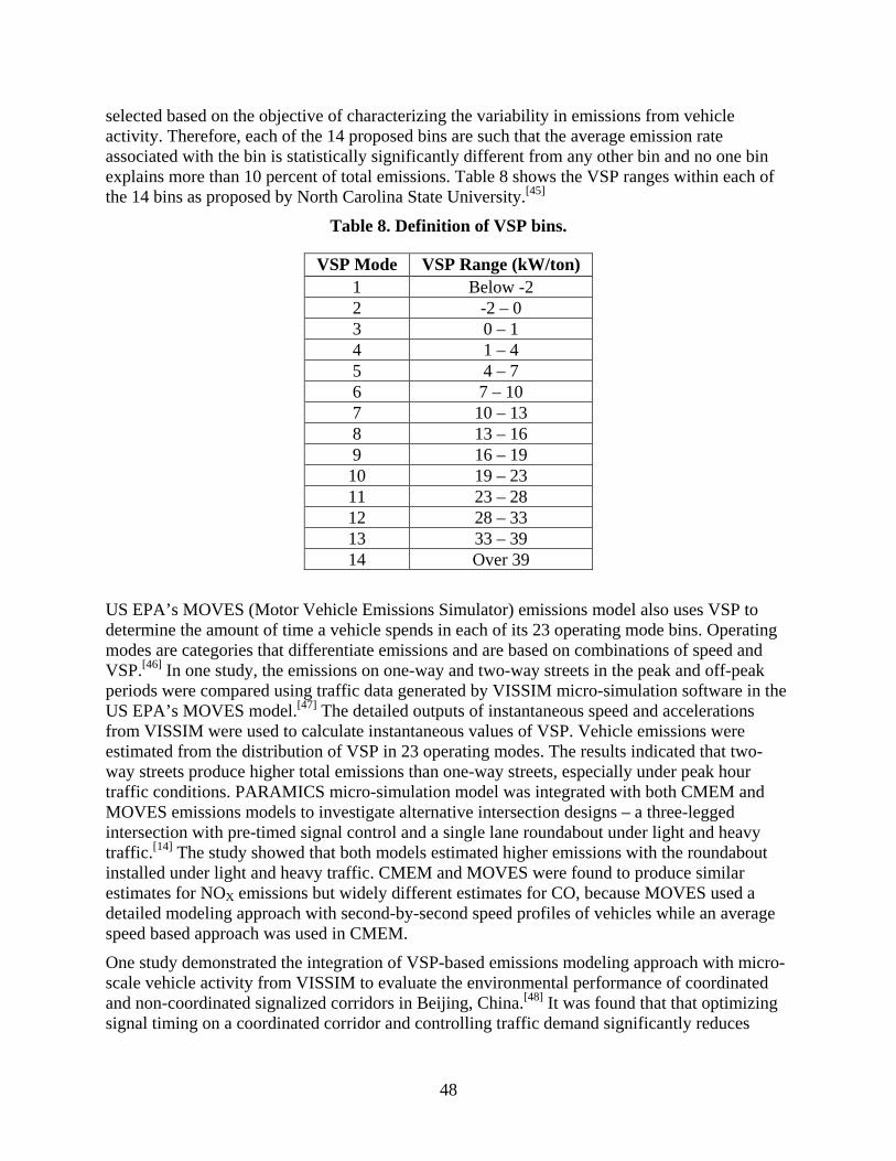
48

selected based on the objective of characterizing the variability in emissions from vehicle activity. Therefore, each of the 14 proposed bins are such that the average emission rate associated with the bin is statistically significantly different from any other bin and no one bin explains more than 10 percent of total emissions. Table 8 shows the VSP ranges within each of the 14 bins as proposed by North Carolina State University.[45]

Table 8. Definition of VSP bins.

VSP Mode VSP Range (kW/ton) 1 Below -2 2 -2 – 0 3 0 – 1 4 1 – 4 5 4 – 7 6 7 – 10 7 10 – 13 8 13 – 16 9 16 – 19 10 19 – 23 11 23 – 28 12 28 – 33 13 33 – 39 14 Over 39

US EPA’s MOVES (Motor Vehicle Emissions Simulator) emissions model also uses VSP to determine the amount of time a vehicle spends in each of its 23 operating mode bins. Operating modes are categories that differentiate emissions and are based on combinations of speed and VSP.[46] In one study, the emissions on one-way and two-way streets in the peak and off-peak periods were compared using traffic data generated by VISSIM micro-simulation software in the US EPA’s MOVES model.[47] The detailed outputs of instantaneous speed and accelerations from VISSIM were used to calculate instantaneous values of VSP. Vehicle emissions were estimated from the distribution of VSP in 23 operating modes. The results indicated that two-way streets produce higher total emissions than one-way streets, especially under peak hour traffic conditions. PARAMICS micro-simulation model was integrated with both CMEM and MOVES emissions models to investigate alternative intersection designs – a three-legged intersection with pre-timed signal control and a single lane roundabout under light and heavy traffic.[14] The study showed that both models estimated higher emissions with the roundabout installed under light and heavy traffic. CMEM and MOVES were found to produce similar estimates for NOX emissions but widely different estimates for CO, because MOVES used a detailed modeling approach with second-by-second speed profiles of vehicles while an average speed based approach was used in CMEM.

One study demonstrated the integration of VSP-based emissions modeling approach with micro-scale vehicle activity from VISSIM to evaluate the environmental performance of coordinated and non-coordinated signalized corridors in Beijing, China.[48] It was found that that optimizing signal timing on a coordinated corridor and controlling traffic demand significantly reduces

49

vehicle emissions. The VSP modal emissions analysis was also applied to quantify emissions at single-lane roundabouts in Raleigh, NC and Lisbon, Portugal by means of a hybrid approach based on field data for vehicle activity and an existing emissions model.[1] Empirical data showed that vehicles at a roundabout follow one of three possible trajectories: (1) a vehicle travels through the roundabout by slowing down in response to the geometrics without stopping fully; (2) the vehicle comes to a full stop at the entry line of an approach to negotiate a gap in the circulating traffic, accelerate to the circulation speed before eventually accelerating back to original speed; and (3) the vehicle enters a queue and experiences stop-and-go motion until passing the yield line. Complete speed profiles for each possible trajectory through the roundabout were developed using the modeling approach of North Carolina State University[45] to obtain VSP values. VSP modal emission factors in g/s were then used to estimate emissions per vehicle, which, coupled with the proportion of vehicles following each of the three speed profiles and the approach entry flow rate, was used to determine total hourly emissions at the roundabout.

Use of VSP in estimating emissions was also demonstrated in a study of a regional road network in North Carolina created using the AIMSUN micro-simulation system.[50] This study used the modal emission factors estimated from data collected on the same road network using Portable Emissions Measurement System (PEMS) with the VSP distributions from AIMSUN-simulated data. The study found that for freeway segments of the routes, the total empirical emissions and emissions calculated from the modal model were within ± 10 percent of each other. The arterial sections did not share the same trend because of greater differences in VSP distributions between simulation and real world data. The authors recommended that for evaluating emissions on arterial segments using the VSP modal approach, the internal behavioral model parameters in AIMSUN should be calibrated appropriately to generate vehicle activity that is more representative of the real world.

Traffic on arterial roads experience larger and more frequent speed fluctuations in comparison to freeway traffic. The highest fuel consumption on arterials is associated with driving in congested traffic, characterized by higher speed fluctuations and frequent stops at intersections.[16] However, low traffic and continuous progression along streets do not guarantee the lowest fuel consumption and emissions. The authors suggested that the best flow of traffic on arterial streets in terms of fuel consumption and emissions is the one with the fewest stops, shortest delays, and moderate speeds maintained throughout the commute. To investigate the emissions on existing arterial roads and study the effects of improvements to traffic flow using micro-simulation models, it is necessary to ensure that the simulated traffic on arterials accurately represents what is or can be expected to in the real world. In a study that linked the output from macroscopic transportation models to the microscopic VSP-based emissions modeling approach, it was shown that arterial speed profiles can be grouped together with respect to the average link speed. Average emission rates increased with average speed for arterials.[48]

A recent study investigated the amount of error in emissions estimates using VSP distributions of vehicle activity data from VISSIM and the sensitivity of VSP distributions to modeling parameters[18]. It was observed that second-by-second empirical vehicle activity data and simulated vehicle activity data from a calibrated and validated VISSIM model did not yield the same VSP distributions. The parameters had been calibrated using GPS data and Remote Traffic Microwave Sensors (RTMS) data from freeways or expressways with flat terrain in Beijing and

50

included: (1) Desired Speed distribution, (2) Desired Acceleration Distribution, (3) Maximum Acceleration, (4) Desired Deceleration Distribution, (5) Maximum Deceleration, (6) Maximum Deceleration for Co-operative Braking (7) Safety Distance Reduction Factor and (8) Maximum Look Ahead Distance. The differences between the simulated time-varying speeds and the RTMS-collected field speeds were less 15 percent, while the differences between traffic flow measures were less than 10 percent. The validation was done using the link average speed and flow. Emission rates per unit distance were calculated using MOVES emission factors and the VSP distributions for the simulated activity. The simulated vehicle activity produced high errors, especially for NOX emissions. Simulation model overestimated emissions for low speed conditions by up to 248 percent and underestimated emissions for high speed conditions by up to 16 percent. It was found that these errors were systematic errors in the traffic simulation models, because they remained statistically the same when a sensitivity analysis was performed on eight parameters by increasing and decreasing their values by 10 percent.

It has been demonstrated that calibrating the distributions of acceleration, deceleration and speed of buses in AIMSUN micro-simulation model affect the emissions estimates from the vehicle activity.[48] Second-by-second bus performance data was collected automatically by the iBus system in London and used to modify input distributions of the relevant parameters pertaining to the motion of simulated buses. Emissions were estimated using the emissions model developed,[52] which is already embedded in AIMSUN. Emission functions which differ by vehicle, fuel, and pollutant types were used to modify the emissions calculated at each simulation step using the same formula for all pollutants.[52] The study showed that under the calibrated parameters, the buses produced significantly more emissions under heavy traffic flow conditions due to more stop-and-go cycles than under the default parameters. The emissions were less sensitive however, under low flow conditions.

The VSP modal approach was also used to compare numerically simulated data from five car following models - optimal velocity model (OVM), generalized force model (GFM), full velocity difference model (FVDM), Weidemann model, and Fritzsche model.[51] It was observed that the Fritzsche produced more realistic VSP distributions than the other models. VSP distributions from the Weidemann model showed larger differences with the field observed VSP distributions at higher speed and overestimated emission. The FVDM model gave the lowest RMSE when the acceleration distributions were compared between simulated and field data. However, RMSE increased as speeds increased to more than 40 km/h. The Fritzsche model had slightly higher RMSE than the FVDM model. The study found that speed-specific VSP distributions were highly correlated to the acceleration distribution and therefore, improving the acceleration distribution for certain speed bins is a promising method of improving calibration of car following models for estimating emissions using the VSP modal approach. Popular micro-simulation models, PARAMICS and VISSIM are based on the Fritzsche and Wiedemann models respectively. However, the exact differences between the models that are published in literature and the simulation models are not in the public domain.[53]

51

APPENDIX B. DATA COLLECTION DETAILS

This appendix includes the details for speed trajectories used in the computation engine to develop the emission factors reference tables and VSP distribution models for signalized intersections and for roundabouts. From 2008 to the present, data have been collected for Passenger Cars (PCs) and Passenger Trucks (PTs) in the Research Triangle Park, NC area representing vehicle activity for multiple road functional classes (i.e. feeder/collector streets, minor arterials, major arterials, freeway, ramp) and a wide range of speed and acceleration.2,3] The second-by-second speed trajectories and emissions generated from vehicle exhaust were collected from a fleet size of 95 vehicles. Each of these vehicles were equipped with a PEMS device and three GPS devices to report the second-by-second emissions and engine activity such as sped, deceleration rate, etc. The vehicles were set to drive through a certain route in the Research Triangle Park, NC, shown in figure 37. The data from PEMS were then analyzed to calculate the emission factors. Fleet average VSP modal rates were estimated for each of four vehicle groups: T1 PC (n=24); T2 PC (n=39); T1 PT (n=10), and T2 PT (n=22), with T1 indicating Tier 1 emission standards, and T2 indicating Tier 2 emission standards. The mean values for pollutants NOX, HC, CO2 and CO for VSP modes (emission factors) are shown in figure 18 and table 7 in the report.

The second-by-second data from GPS devices were also used to calculate the VSP distribution for signalized intersections. For every second of the speed trajectory, the VSP value of that speed and deceleration rate was calculated and then the associated VSP bin was identified. Last, for each compete speed profile through a certain intersection, the percent of time spent in each VSP mode was calculated from those data, and the VSP distribution models developed. Table 9 shows the list of the intersections that the data was collected from.

Table 9. List of the signalized intersections used for data collection.

Intersections Approaches No. of Lanes1 A Profiles

B Profiles

C Profiles

W. Morgan and Mayo (1) 4 EB: 1TR, 1T; WB 1LT

11 0 0

W. Morgan and St. Mary’s (2)

4 EB: 1LT, 1TR; WB: 1LTR

9 2 0

W. Morgan and Glenwood (3)

3 EB: 1LT, 1T; WB: 1TR

11 1 0

W. Morgan and S. West (4) 4 EB: 1LT, 1TR; WB: 1LTR

10 2 0

W. Morgan and S. Dawson (5)

2 EB: 1T, 1TR; WB: 1T

11 1 0

Wake Forest and McNeill (8)

3 NB: 1L, 3T; SB: 1L, 1T,

1TR

18 4 0

Wake Forest and Hodges (9) 4 NB: 1L, 2T, 1TR; SB: 1L,

1T, 1TR

21 1 0

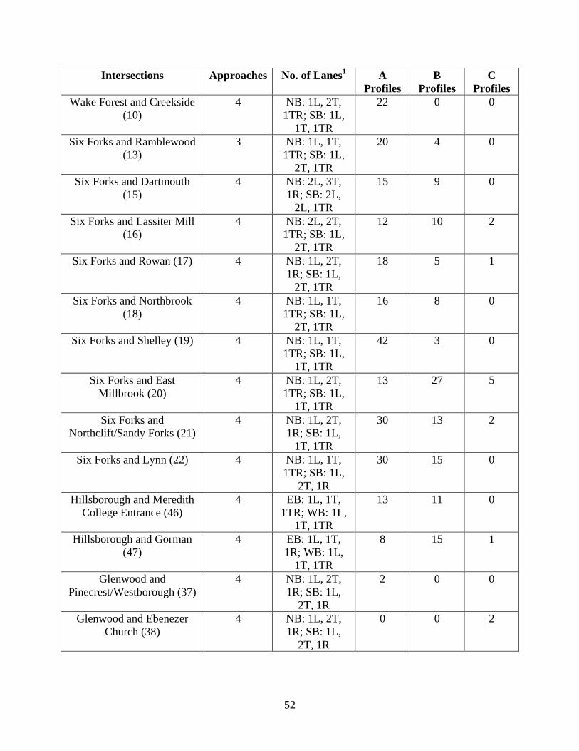
52

Intersections Approaches No. of Lanes1 A Profiles

B Profiles

C Profiles

Wake Forest and Creekside (10)

4 NB: 1L, 2T, 1TR; SB: 1L,

1T, 1TR

22 0 0

Six Forks and Ramblewood (13)

3 NB: 1L, 1T, 1TR; SB: 1L,

2T, 1TR

20 4 0

Six Forks and Dartmouth (15)

4 NB: 2L, 3T, 1R; SB: 2L,

2L, 1TR

15 9 0

Six Forks and Lassiter Mill (16)

4 NB: 2L, 2T, 1TR; SB: 1L,

2T, 1TR

12 10 2

Six Forks and Rowan (17) 4 NB: 1L, 2T, 1R; SB: 1L,

2T, 1TR

18 5 1

Six Forks and Northbrook (18)

4 NB: 1L, 1T, 1TR; SB: 1L,

2T, 1TR

16 8 0

Six Forks and Shelley (19) 4 NB: 1L, 1T, 1TR; SB: 1L,

1T, 1TR

42 3 0

Six Forks and East Millbrook (20)

4 NB: 1L, 2T, 1TR; SB: 1L,

1T, 1TR

13 27 5

Six Forks and Northclift/Sandy Forks (21)

4 NB: 1L, 2T, 1R; SB: 1L,

1T, 1TR

30 13 2

Six Forks and Lynn (22) 4 NB: 1L, 1T, 1TR; SB: 1L,

2T, 1R

30 15 0

Hillsborough and Meredith College Entrance (46)

4 EB: 1L, 1T, 1TR; WB: 1L,

1T, 1TR

13 11 0

Hillsborough and Gorman (47)

4 EB: 1L, 1T, 1R; WB: 1L,

1T, 1TR

8 15 1

Glenwood and Pinecrest/Westborough (37)

4 NB: 1L, 2T, 1R; SB: 1L,

2T, 1R

2 0 0

Glenwood and Ebenezer Church (38)

4 NB: 1L, 2T, 1R; SB: 1L,

2T, 1R

0 0 2

53

Intersections Approaches No. of Lanes1 A Profiles

B Profiles

C Profiles

Glenwood and Triangle (39) 4 NB: 1L, 2T, 1R; SB: 1L, 2T

2 0 0

Glenwood and Brier Creek (40)

4 NB: 2L, 3T, 1R; SB: 2L,

3T, 1R

0 0 2

TW Alexander and S. Miami (42)

4 NB: 1L, 3T, 1R; SB: 1L,

2T, 1R

1 6 0

TW Alexander and N. Entrance (43)

4 EB: 1L, 2T, 1R; WB: 1L,

2T, 1R

4 2 1

TW Alexander and Moore (44)

4 EB: 1L, 1T, 1TR; WB: 1L,

2T, 1R

2 1 4

TW Alexander and E. Cornwallis (45)

4 NB: 1L, 2T, 1R; SB: 1L,

2T, 1R

2 2 3

Hillsborough and Friendly/Dixie (48)

4 EB: 1LT, 1RT; WB: 1L, 1T,

1TR

6 0 0

Hillsborough and Brooks (49)

4 EB: 1L, 1T, 1R; WB: 1L,

1T, 1TR

4 2 0

Hillsborough and Gardner (50)

4 EB: 1L, 1T; WB: 1TR

4 1 1

Hillsborough and Horne (51) 4 EB: 1TR; WB: 1T

2 1 3

1 EB = eastbound; WB = westbound; NB = northbound; SB = southbound; L = Left; R = Right; T = Through.

54

Figure 37. Map. Research Triangle Park, location of the signalized intersections.

As for the roundabouts, same as signalized intersections, second-by-second data were collected from GPS devices as vehicles were driving through the roundabouts to develop the VSP distribution models. The speed data were available from a previous project on roundabout corridors, NCHRP Project 03-100 (NCHRP Report 772).

These locations include the following roundabout corridors:

- Carmel, IN: Old Meridian St. - Gig-Harbor, WA: Borgen Blvd. - Malta, NY: SR 67 - San Diego, CA: La Jolla Blvd. - Avon, CO: Avon Rd. - Golden, CO: Golden Rd. - Carmel, IN: Spring Mill Rd. - Whatcom County, WA: SR 539

For more information on the location of the roundabouts can be found in the NCHRP Report 772, Evaluating the Performance of Corridors with Roundabouts.

55

APPENDIX C. SIMULATION EXPERIMENT DETAILS

This appendix exhibits the results of the VISSIM simulation used develop the regression models presented in the report. Table 10 lists the coefficients of variables used for predicting the likelihood for Type A trajectories. Table 11 lists the probability functions for predicting the proportion of Type C trajectories.

Table 10. Coefficients of variables used for predicting the likelihood of a no-stop (Type A) speed profile at a signalized intersection approach (table 3).

Arrival Type

Platoon Ratio,

Rp

b0 b1 b2

1 0.33 Min[1,Rp(g/c)] -0.0195+0.580*g/C 3 2 0.67 Min[1,Rp(g/c)] -0.0195+0.580*g/C 3 3 1 Min[1,Rp(g/c)] -0.0195+0.580*g/C 3 4 1.33 Min[1,Rp(g/c)] -0.9809(g/C)2+1.2748(g/C)-0.0149 5(Rp g/C) 5 1.67 Min[1,Rp(g/c)] -1.7314(g/C)2+1.9424(g/C)-0.0852 4(Rp g/C) 6 2 Min[1,Rp(g/c)] -2.2578(g/C)2+2.1815(g/C)-0.0487 4(Rp g/C)

Table 11. Functions for predicting the proportion of a Type C profile at a signalized intersection approach (table 4).

Arrival Type

d/c Fraction of Type C Trajectories

R2

1,2 Less than or equal to 0.7 0 0.95 1,2 Between 0.1 and 1.2 Figure 15 0.95 1,2 Greater than or equal to 1.2 1 0.95 3-6 Less than or equal to 1 0 0.90 3-6 Between 1 and 1.213 Figure 16 0.90 3-6 Greater than or equal to 1.213 1 0.90

For the VISSIM simulation two sets of eight different model were developed. The design of the VISSIM network is a simple two-lane link with two pre-timed signals located at a specific distance from each other on this link. Eight of these models (the first set) simulated a high speed environment with a Free Flow Speed (FFS) value of 72 km/h (45 mph) and the second set of eight models simulated an environment with a low FFS of 56 km/h (35 mph). The signals in the models have a 120 s cycle length. Each of the eight models in each set are set for a certain g/C ratio and effective green (g) values are 30 s, 40 s, 50 s, 60 s, 70 s, 80 s, and 90 s. The offset for the signals was set to simulated three arrival patterns, poor progression, random arrival and good progression. The volume during the simulation period changed to include d/c ratio range from 0.1 to approximately 1.4. All the scenarios resulted in 48 simulation models and each model was run 10 times resulting in 480 simulation runs, each for a period of 1 h. Then a macro was

56

developed to process each vehicle trajectory type in the simulation run and calculate the percentage of Type A, B and C trajectories during the simulation period.

57

APPENDIX D. COMPUTATIONAL ENGINE DETAILS

This appendix contains screenshots of the computational engine developed for this project. Figure 38, figure 39, figure 40, figure 41, figure 42, figure 43, and figure 44 are all screenshots from the engine.

Figure 38. Screenshot. Sheet 1 – instructions.

1234567

Rp Arrival Type Progression Quality from upstream signal0.33 1 Very poor0.67 2 Unfavorable

1 3 Random Arrivals1.33 4 Favorable1.67 5 Highly Favorable

2 6 Exceptionally Favorable

1 Speeds less than 35 MPH2 Speeds more than 35 MPH

Approach Speed Bin

Use table below to enter the HCM arrival time

Instructions

The results are shown in "Summary Output" sheet

HCM Arrival Type Describing Progression Quality at Traffic Signals

Use the "Signal Input" sheet and "Roundabout Input" sheet to enter the intersection informationYou can choose to do the emissions analysis for only one time period (AM or PM or Off Peak) or a combination of time periodsPlease note that some data are required for each time period individually, such as appraoch demandApproach speed bin is 1 for speeds less than 35 MPH and 2 for speeds more than 35 MPHThe sume of Tier1 PC, Tier 2 PC, Tier 1 PT and Tier 2 PT should equal 100%

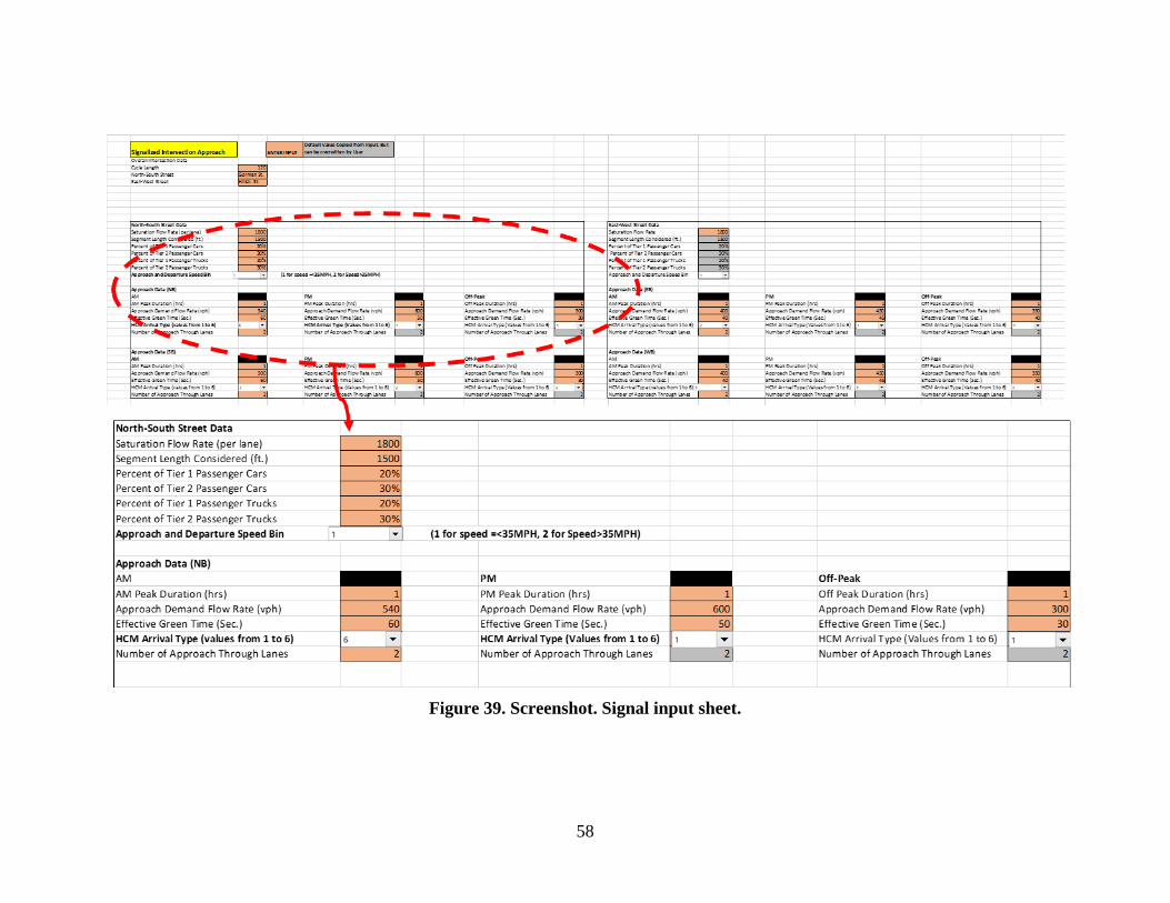
58

Figure 39. Screenshot. Signal input sheet.

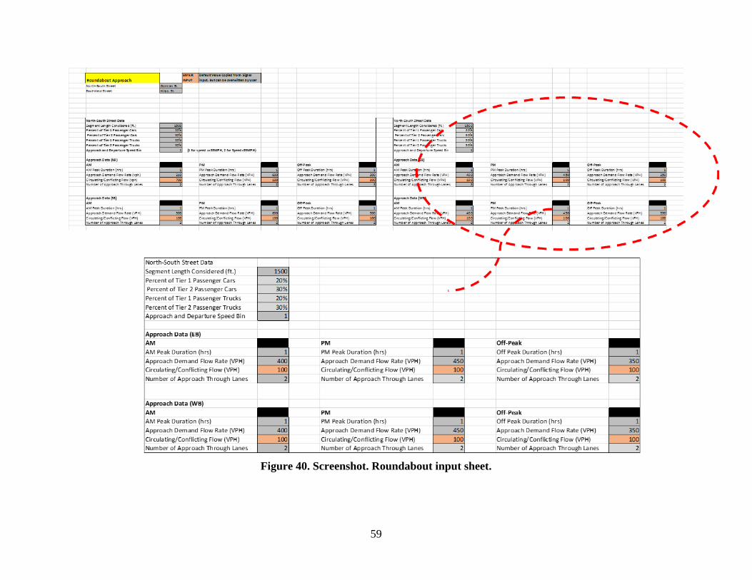
59

Figure 40. Screenshot. Roundabout input sheet.

60

Figure 41. Screenshot. Sample signal calculations sheet.

Signal- NB AM Peak 1 Average Travel SpeedBin1 Bin2 Travel Time Over the Segment for Selected Speed Bin g/C= 0.333 d/c= 0.292

35.122 43.245 A 29.11 seconds Arrival Type Rp b0 b1 b2 R-squared bo b1 b2 %A Calc. %C Calc. %A %B %C

15.782 28.515 B 64.79 seconds 1 0.33 Min[1,Rp(g/c)] -0.0195+0.580*g/C 3 0.11 0.173833333 3 0.105687 0 0.105687 0.894313 0

1- Approach Demand flow Rate (vph) 350 10.318 16.271 C 99.09 seconds 2 0.67 Min[1,Rp(g/c)] -0.0195+0.580*g/C 3 0.223333333 0.173833333 3 0.21902 0 0.21902 0.78098 0

2-Saturation Flow Rate 1800 3 1 Min[1,Rp(g/c)] -0.0195+0.580*g/C 3 0.333333333 0.173833333 3 0.32902 0 0.32902 0.67098 0

3- Cycle Length (sec) 120 4 1.33 Min[1,Rp(g/c)] -0.9809(g/C)2+1.2748(g5(Rp g/C) 0.443333333 0.301044444 0.55 0.290465 0 0.290465 0.709535 0

4- Effective Green Time (sec) 40 5 1.67 Min[1,Rp(g/c)] -1.7314(g/C)2+1.9424(g4(Rp g/C) 0.556666667 0.369888889 0.893333 0.433629 0 0.433629 0.566371 0

5-HCM Arrival Type 3 6 2 Min[1,Rp(g/c)] -2.2578(g/C)2+2.1815(g4(Rp g/C) 0.666666667 0.4276 1.333333 0.583958 0 0.583958 0.416042 0

6-Number of approach through lanes 27- Approach and Departure Speed Bin 18- Segment Length Considered (ft) 15009-Percent of Tier 1 Passenger Cars 20% AM

10- Percent of Tier 2 Passenger Cars 30%11- Percent of Tier 1 Passenger Trucks 20% Appraoch Signal Variables 3 % A profiles 33%12- Percent of Tier 2 Passenger Trucks 30% Approach Signal C 1200 %B profiles 67%

g/C Ratio 0.333 %C-profiles 0%demand/capacity 0.292 Overall Average Travel Time (sec) 53.05

VSP Mode Distribution for Each Speed Bin time Spent in Each VSP Mode for Each Profile Multiplied by % of time inEach profile gives travel time @VSP

constant from another sheet>>>>

VSP Mod A B C VSP ModA B C VSP Mode A B C A B C Sum

1 22.34% 12.20% 9.19% 1 18.03% 18.03% 8.10% 1 6.503 7.904 9.105 1 2.139 5.303 0.000 7.443

2 1.63% 2.24% 5.37% 2 1.86% 1.86% 2.93% 2 0.473 1.450 5.321 2 0.156 0.973 0.000 1.129

3 1.57% 41.23% 70.41% 3 2.15% 20.63% 59.01% 3 0.456 26.712 69.768 3 0.150 17.923 0.000 18.073

4 32.70% 9.53% 6.80% 4 13.76% 2.15% 5.87% 4 9.520 6.174 6.740 4 3.132 4.143 0.000 7.275

5 16.32% 7.91% 1.55% 5 27.68% 13.76% 6.01% 5 4.750 5.125 1.537 5 1.563 3.439 0.000 5.001

6 4.70% 6.30% 2.39% 6 15.60% 15.60% 6.70% 6 1.367 4.082 2.365 6 0.450 2.739 0.000 3.188

7 9.45% 4.84% 0.95% 7 6.43% 6.43% 3.63% 7 2.752 3.134 0.946 7 0.905 2.103 0.000 3.008

8 2.76% 3.78% 1.79% 8 5.52% 6.52% 2.93% 8 0.804 2.449 1.774 8 0.264 1.643 0.000 1.908

9 2.75% 2.53% 0.60% 9 4.02% 5.02% 2.51% 9 0.801 1.639 0.591 9 0.263 1.100 0.000 1.363

10 2.36% 2.36% 0.48% 10 3.27% 5.27% 1.47% 10 0.687 1.529 0.473 10 0.226 1.026 0.000 1.252

11 2.36% 2.12% 0.12% 11 0.95% 1.09% 0.49% 11 0.687 1.373 0.118 11 0.226 0.922 0.000 1.148

12 0.18% 1.64% 0.00% 12 0.29% 1.23% 0.28% 12 0.053 1.063 0.000 12 0.017 0.713 0.000 0.730

13 0.12% 1.78% 0.00% 13 0.17% 1.17% 0.07% 13 0.035 1.153 0.000 13 0.012 0.774 0.000 0.785

14 0.78% 1.55% 0.36% 14 0.25% 1.24% 0.00% 14 0.228 1.004 0.355 14 0.075 0.674 0.000 0.749 SUM 29.114 64.790 99.094 SUM 9.579 43.473 0.000 53.052

VSP Mode

Combined NOx EF from Emmissio

NOx emissions due to all

Overall NOx emissions per

Overall NOx emissions per

Combined HC EF from Emmission Factors Tab

HC emissions due to all profiles (

Overall HC emissions per hour (mgrams/hr)

Overall HC emissions per mile (grams/

Combined CO EF from Emmission Factors Tab

CO emissions due to all profiles ( mgrams

Overall CO emissions per hour (mgrams/hr)

Overall CO emissions per mile (grams/VMT)

Combined CO2 EF from Emmission Factors Tab

CO2 emissions due to all profiles (

Overall CO2 emissions per

Overall CO2 emissions per mile

1 0.456 3.393 1187.607 4.180 0.361 2.688 940.960 3.312 1.177 8.758 3065.467 10.790 2.805 20.880 7307.908 25.7242 0.751 0.848 296.657 1.044 0.402 0.454 158.757 0.559 1.262 1.425 498.590 1.755 2.882 3.252 1138.349 4.0073 0.954 17.237 6032.788 21.235 0.163 2.955 1034.111 3.640 0.788 14.248 4986.747 17.553 1.312 23.720 8301.867 29.2234 1.491 10.844 3795.333 13.360 0.739 5.376 1881.499 6.623 2.087 15.182 5313.649 18.704 4.971 36.162 12656.771 44.5525 1.948 9.743 3410.172 12.004 1.135 5.675 1986.375 6.992 3.017 15.089 5281.194 18.590 6.972 34.869 12204.133 42.9596 2.380 7.589 2656.293 9.350 1.516 4.833 1691.561 5.954 3.784 12.066 4223.083 14.865 9.392 29.947 10481.441 36.8957 2.735 8.225 2878.893 10.134 1.922 5.781 2023.374 7.122 4.810 14.469 5064.227 17.826 10.330 31.071 10874.728 38.2798 3.089 5.892 2062.362 7.260 2.309 4.405 1541.815 5.427 5.445 10.386 3635.053 12.795 11.365 21.680 7588.127 26.7109 3.448 4.701 1645.273 5.791 2.903 3.957 1385.107 4.876 6.536 8.910 3118.434 10.977 13.456 18.343 6420.046 22.599

10 3.793 4.748 1661.917 5.850 3.163 3.960 1386.101 4.879 8.639 10.815 3785.387 13.325 15.247 19.089 6681.203 23.51811 4.269 4.899 1714.636 6.036 3.898 4.474 1565.903 5.512 9.757 11.197 3918.992 13.795 19.566 22.455 7859.145 27.66412 4.770 3.483 1219.201 4.292 4.803 3.507 1227.573 4.321 13.698 10.002 3500.873 12.323 27.264 19.909 6968.093 24.52813 5.319 4.177 1461.927 5.146 5.132 4.030 1410.481 4.965 19.202 15.080 5278.008 18.579 33.660 26.434 9251.730 32.56614 6.154 4.608 1612.655 5.677 7.088 5.307 1857.558 6.539 44.693 33.465 11712.676 41.229 56.470 42.283 14798.918 52.092

SUM 90.388 31635.71 111.358 SUM 57.403 20091.174 70.721 SUM 181.093 63382.381 223.106 SUM 350.093 ######### 431.314

Bin 1, Speed<35 MPH Bin 2, Speed >35 MPH

North Bound

INPUT Values Copied from Signal Input Sheet

0.711

0.4921

0.5017

61

Figure 42. Screenshot. Sample roundabout calculations sheet.

Roundabout- SB AM Peak 1 Average Travel SpeedBin1 Bin2 Travel Time Over the Segment for Selected Speed Bin

33.804 42.942 A 30.25 seconds26.562 36.414 B 38.50 seconds

1- Approach Demand flow Rate (vph) 350 175 20.707 29.773 C 49.38 seconds2-Cirulating/ Conflicting flow rate (vph) 100 1006-Number of approach through lanes 27- Approach and Departure Speed Bin 18- Segment Length Considered (ft) 15009-Percent of Tier 1 Passenger Cars 20%10- Percent of Tier 2 Passenger Cars 30%11- Percent of Tier 1 Passenger Trucks 20% 3 % A profiles 90%12- Percent of Tier 2 Passenger Trucks 30% %B profiles 8%

%C-profiles 2%Overall Average Travel Time (sec) 31.22

VSP Mode Distribution for Each Speed Bin time Spent in Each VSP Mode for Each Profile Multiplied by % of time inEach profile gives travel time @VSP

constant from another sheet>>>>

VSP Mod A B C VSP ModA B C VSP Mode A B C A B C Sum

1 35.39% 34.26% 24.28% 1 22.98% 22.98% 15.15% 1 10.705 13.188 11.987 1 9.685 1.033 0.203 10.921

2 7.23% 9.24% 6.83% 2 2.66% 3.66% 3.79% 2 2.187 3.557 3.373 2 1.979 0.279 0.057 2.314

3 3.27% 15.77% 21.47% 3 15.42% 15.42% 14.39% 3 0.988 6.071 10.604 3 0.894 0.476 0.180 1.550

4 19.46% 8.89% 11.06% 4 5.58% 13.10% 6.82% 4 5.886 3.422 5.460 4 5.325 0.268 0.093 5.686

5 14.25% 7.34% 7.76% 5 13.01% 10.30% 2.27% 5 4.310 2.826 3.834 5 3.900 0.221 0.065 4.186

6 3.90% 6.46% 6.93% 6 10.24% 13.25% 9.09% 6 1.180 2.487 3.421 6 1.067 0.195 0.058 1.320

7 9.09% 5.26% 5.65% 7 6.47% 6.47% 7.58% 7 2.749 2.025 2.790 7 2.487 0.159 0.047 2.693

8 3.48% 4.32% 5.55% 8 6.40% 5.41% 8.33% 8 1.053 1.663 2.742 8 0.952 0.130 0.047 1.129

9 1.43% 1.97% 3.64% 9 5.46% 4.46% 4.55% 9 0.433 0.758 1.796 9 0.391 0.059 0.030 0.481

10 1.08% 3.10% 2.41% 10 5.01% 3.58% 5.30% 10 0.327 1.193 1.189 10 0.296 0.093 0.020 0.409

11 0.39% 1.94% 2.06% 11 2.93% 0.93% 6.82% 11 0.118 0.747 1.019 11 0.107 0.059 0.017 0.183

12 0.20% 0.72% 1.03% 12 1.75% 0.19% 5.30% 12 0.060 0.277 0.510 12 0.055 0.022 0.009 0.085

13 0.10% 0.43% 0.54% 13 1.06% 0.13% 3.03% 13 0.030 0.166 0.267 13 0.027 0.013 0.005 0.045

14 0.74% 0.30% 0.79% 14 1.03% 0.12% 7.58% 14 0.222 0.115 0.388 14 0.201 0.009 0.007 0.217 SUM 30.249 38.495 49.379 SUM 27.366 3.015 0.838 31.219

VSP Mode

Combined NOx EF from Emmissio

NOx emissions due to all profiles (

Overall NOx emissions per hour

Overall NOx emissions per mile

Combined HC EF from Emmission Factors Tab

HC emissions due to all profiles (

Overall HC emissions per hour (mgrams/hr)

Overall HC emissions per mile (grams/

Combined CO EF from Emmission Factors Tab

CO emissions due to all profiles ( mgrams

Overall CO emissions per hour (mgrams/hr)

Overall CO emissions per mile (grams/VMT)

Combined CO2 EF from Emmission Factors Tab

CO2 emissions due to all profiles (

Overall CO2 emissions per

Overall CO2 emissions per mile

1 0.456 4.979 1742.577 6.134 0.361 3.945 1380.671 4.860 1.177 12.851 4497.960 15.833 2.805 30.637 10722.895 37.7452 0.751 1.738 608.378 2.141 0.402 0.930 325.575 1.146 1.262 2.921 1022.498 3.599 2.882 6.670 2334.503 8.2173 0.954 1.478 517.291 1.821 0.163 0.253 88.671 0.312 0.788 1.222 427.596 1.505 1.312 2.034 711.856 2.5064 1.491 8.475 2966.350 10.442 0.739 4.202 1470.539 5.176 2.087 11.866 4153.034 14.619 4.971 28.264 9892.260 34.8215 1.948 8.155 2854.175 10.047 1.135 4.750 1662.514 5.852 3.017 12.629 4420.143 15.559 6.972 29.184 10214.360 35.9556 2.380 3.142 1099.748 3.871 1.516 2.001 700.334 2.465 3.784 4.995 1748.424 6.154 9.392 12.399 4339.485 15.2757 2.735 7.365 2577.658 9.073 1.922 5.176 1811.657 6.377 4.810 12.955 4534.329 15.961 10.330 27.820 9736.845 34.2748 3.089 3.488 1220.711 4.297 2.309 2.607 912.600 3.212 5.445 6.147 2151.587 7.574 11.365 12.833 4491.410 15.8109 3.448 1.659 580.742 2.044 2.903 1.397 488.910 1.721 6.536 3.145 1100.733 3.875 13.456 6.475 2266.123 7.977

10 3.793 1.552 543.180 1.912 3.163 1.294 453.033 1.595 8.639 3.535 1237.215 4.355 15.247 6.239 2183.682 7.68711 4.269 0.779 272.683 0.960 3.898 0.712 249.029 0.877 9.757 1.781 623.247 2.194 19.566 3.571 1249.859 4.40012 4.770 0.406 142.061 0.500 4.803 0.409 143.036 0.503 13.698 1.165 407.921 1.436 27.264 2.320 811.920 2.85813 5.319 0.239 83.509 0.294 5.132 0.230 80.570 0.284 19.202 0.861 301.494 1.061 33.660 1.510 528.484 1.86014 6.154 1.334 467.034 1.644 7.088 1.537 537.959 1.894 44.693 9.692 3392.055 11.940 56.470 12.245 4285.848 15.086

SUM 44.789 15676.10 55.180 SUM 29.443 10305.099 36.274 SUM 85.766 30018.235 105.664 SUM 182.199 63769.530 224.469

North Bound

INPUT Values Copied from Roundabout Input Sheet

Bin 1, Speed<35 MPH Bin 2, Speed >35 MPH

62

Figure 43. Screenshot. Summary output sheet.

Summary Output

AM PM Off Peak AM PM Off Peak AM PM Off Peak AM PM Off Peak AM PM Off Peak AM PM Off Peak AM PM Off Peak AM PM Off Peak AM PM Off Peak AM PM Off PeakNB 35.95 26.88 25.02 30.65 60.39 62.01 NB 40% 83% 92% 96% 12% 8% NB 41% 13% 7% 4% 88% 92% NB 18% 4% 1% 0% 0% 0% NB 0.30 0.57 0.28 0.30 0.40 0.33SB 26.16 26.88 25.02 53.04 55.34 56.03 SB 86% 83% 92% 33% 26% 25% SB 11% 13% 7% 67% 74% 75% SB 3% 4% 1% 0% 0% 0% SB 0.47 0.57 0.28 0.28 0.40 0.33EB 31.37 31.54 31.22 56.26 60.63 61.02 EB 89% 88% 90% 24% 12% 11% EB 9% 10% 8% 76% 88% 89% EB 2% 3% 2% 0% 0% 0% EB 0.38 0.43 0.33 0.33 0.33 0.29WB 31.37 31.54 31.22 53.13 51.67 53.05 WB 89% 88% 90% 33% 37% 33% WB 9% 10% 8% 67% 63% 67% WB 2% 3% 2% 0% 0% 0% WB 0.38 0.43 0.33 0.33 0.33 0.29

AM PM Off Peak AM PM Off Peak AM PM Off Peak AM PM Off Peak AM PM Off Peak AM PM Off Peak Roundabout SignalNB 79.97 55.91 51.12 53.22 95.78 98.10 NB 16794.51 33548.67 15335.86 28738.28 57470.70 29431.16 NB 59.12 118.09 53.98 101.16 78.27 103.60 NB 231.19 283.03SB 54.06 55.91 51.12 85.27 88.55 89.55 SB 27028.78 33548.67 15335.86 42635.71 53131.11 26865.69 SB 95.14 118.09 53.98 150.08 187.02 94.57 SB 267.21 431.67EB 45.04 45.32 44.79 95.73 103.00 103.63 EB 18016.69 20393.18 15676.10 38290.87 46348.00 36271.15 EB 63.42 71.78 55.18 134.78 163.14 127.67 EB 190.38 425.60WB 45.04 45.32 44.79 90.51 88.10 90.39 WB 18016.69 20393.18 15676.10 36205.51 39643.17 31635.71 WB 63.42 71.78 55.18 127.44 139.54 111.36 WB 190.38 378.35

AM PM Off Peak AM PM Off Peak AM PM Off Peak AM PM Off Peak AM PM Off Peak AM PM Off Peak Roundabout SignalNB 28.36 20.38 317.25 20.68 37.06 37.95 NB 5956.51 12229.25 95173.90 11168.82 22237.15 11386.31 NB 20.97 43.05 19.83 39.31 78.27 40.08 NB 83.84 157.67SB 19.76 20.38 317.25 33.02 34.28 34.66 SB 9879.92 12229.25 95173.90 16508.27 20567.30 10399.14 SB 34.78 43.05 19.83 58.11 72.40 36.60 SB 97.65 167.11EB 29.61 29.80 85.77 60.61 64.98 65.37 EB 11844.77 13408.41 30018.24 24245.56 29242.94 22878.42 EB 41.69 47.20 36.27 85.34 102.94 80.53 EB 125.17 268.81WB 29.61 29.80 85.77 57.48 56.03 57.40 WB 11844.77 13408.41 30018.24 22991.65 25211.39 20091.17 WB 41.69 47.20 36.27 80.93 88.74 70.72 WB 125.17 240.40

AM PM Off Peak AM PM Off Peak AM PM Off Peak AM PM Off Peak AM PM Off Peak AM PM Off Peak Roundabout SignalNB 545.03 354.85 317.25 324.42 656.19 674.27 NB 114457.21 212909.96 95173.90 175186.33 393712.50 202279.58 NB 402.89 749.44 335.01 616.66 1385.87 712.02 NB 1487.34 2714.55SB 340.30 354.85 317.25 574.25 599.81 607.61 SB 170151.27 212909.96 95173.90 287122.65 359888.41 182283.58 SB 598.93 749.44 335.01 1010.67 1266.81 641.64 SB 1683.39 2919.12EB 86.24 86.75 85.77 192.64 208.36 209.74 EB 34494.09 39036.49 30018.24 77056.01 93761.66 73407.38 EB 121.42 137.41 105.66 271.24 330.04 258.39 EB 364.49 859.67WB 86.24 86.75 85.77 181.37 176.14 181.09 WB 34494.09 39036.49 30018.24 72546.03 79261.22 63382.38 WB 121.42 137.41 105.66 255.36 279.00 223.11 WB 364.49 757.47

AM PM Off Peak AM PM Off Peak AM PM Off Peak AM PM Off Peak AM PM Off Peak AM PM Off Peak Roundabout SignalNB 149.53 107.38 98.91 109.61 194.40 199.02 NB 31400.49 64427.06 29671.94 59188.65 116640.78 59706.47 NB 110.53 226.78 104.45 208.34 410.58 210.17 NB 441.76 829.09SB 104.09 107.38 98.91 173.46 179.99 181.99 SB 52046.97 64427.06 29671.94 86729.34 107996.09 54595.94 SB 183.21 226.78 104.45 305.29 380.15 192.18 SB 514.43 877.61EB 183.12 184.12 182.20 370.07 397.27 399.65 EB 73247.04 82855.00 63769.53 148028.58 178770.48 139877.00 EB 257.83 291.65 224.47 521.06 629.27 492.37 EB 773.95 1642.70WB 183.12 184.12 182.20 350.56 341.52 350.09 WB 73247.04 82855.00 63769.53 140225.72 153682.83 122532.46 WB 257.83 291.65 224.47 493.59 540.96 431.31 WB 773.95 1465.87

Table 18 Table 19 Table 20

Table 6 Table 7 Table 8

Table 10 Table 11 Table 12

CO: mgrams/vehicle

Roundabout Signal

Table 5

Table 9

Table 13

Table 17

Table 21

CO: grams/ Time Duration Provided by User

d/c (Demand to Capacity Ratio)Roundabout Signal

AM + PM + Off Peak Duration

NOx: grams/ Time Duration Provided by User

HC: grams/ Time Duration Provided by UserAM + PM + Off Peak Duration

Table 1 Table 2 Table 3 Table 4

Table 14 Table 15 Table 16

NOx: mgrams/vehicle

HC: mgrams/vehicleRoundabout Signal

Travel Time (Sec.)Roundabout Signal

% Vehicles with No Stop (A)Roundabout

CO2: grams/ Time Duration Provided by UserAM + PM + Off Peak Duration

Roundabout Signal

Roundabout Signal

CO2: mgrams/vehicleRoundabout Signal

CO: mgrams/hrRoundabout Signal

CO2: grams/hrRoundabout Signal

AM + PM + Off Peak Duration

Signal

NOx: mgrams/hrRoundabout Signal

HC: mgrams/hr

CO2: kilograms/VMTRoundabout Signal

NOx: grams/VMTRoundabout Signal

HC: grams/VMTRoundabout Signal

CO: grams/VMTRoundabout Signal

% Vehicles that Stop Only once (B)Roundabout Signal

% Vehicles that Stop More than Once (C)Roundabout Signal

0.0020.0040.0060.0080.00

100.00120.00140.00160.00

NB

SB

EB

WB

NOx Pollutants: grams/VMTDuring AM Peak HoursRoundabout-AM: NOx Signal-AM: NOx

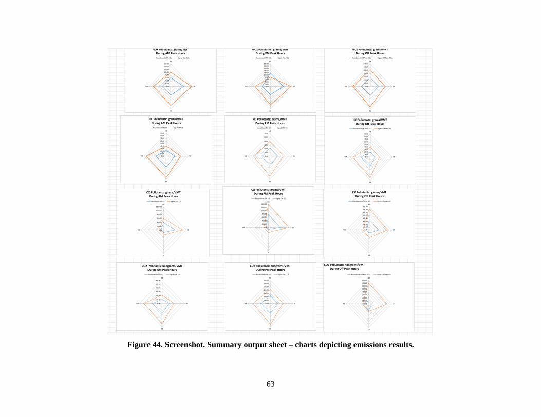
63

Figure 44. Screenshot. Summary output sheet – charts depicting emissions results.

0.0020.0040.0060.0080.00

100.00120.00140.00160.00180.00200.00

NB

SB

EB

WB

NOx Pollutants: grams/VMTDuring PM Peak HoursRoundabout-PM: NOx Siganl-PM: NOx

0.00

20.00

40.00

60.00

80.00

100.00

120.00

140.00NB

SB

EB

WB

NOx Pollutants: grams/VMTDuring Off Peak Hours

Roundabout-Off Peak-NOx Siganl-Off Peak: NOx

0.00

200.00

400.00

600.00

800.00

1000.00

1200.00NB

SB

EB

WB

CO Pollutants: grams/VMTDuring AM Peak Hours

Roundabout-AM:Co Signal-AM: CO

0.00

200.00

400.00

600.00

800.00

1000.00

1200.00

1400.00NB

SB

EB

WB

CO Pollutants: grams/VMTDuring PM Peak Hours

Roundabout-PM: CO Siganl-PM: CO

0.00

100.00

200.00

300.00

400.00

500.00

600.00

700.00

800.00NB

SB

EB

WB

CO Pollutants: grams/VMTDuring Off Peak Hours

Roundabout-Off Peak: CO Siganl-Off Peak: CO

0.0010.0020.0030.0040.0050.0060.0070.0080.0090.00

NB

SB

EB

WB

HC Pollutants: grams/VMTDuring AM Peak Hours

Roundabout-AM:HC Signal-AM: HC

0.00

20.00

40.00

60.00

80.00

100.00

120.00NB

SB

EB

WB

HC Pollutants: grams/VMTDuring PM Peak Hours

Roundabout-PM: HC Siganl-PM: HC

0.0010.0020.0030.0040.0050.0060.0070.0080.0090.00

NB

SB

EB

WB

HC Pollutants: grams/VMTDuring Off Peak Hours

Roundabout-Off Peak: HC Siganl-Off Peak: HC

0.0020.0040.0060.0080.00

100.00120.00140.00160.00

NB

SB

EB

WB

NOx Pollutants: grams/VMTDuring AM Peak HoursRoundabout-AM: NOx Signal-AM: NOx

0.00

100.00

200.00

300.00

400.00

500.00

600.00NB

SB

EB

WB

CO2 Pollutants: Kilograms/VMTDuring AM Peak HoursRoundabout-AM:CO2 Signal-AM: CO2

0.00

100.00

200.00

300.00

400.00

500.00

600.00

700.00NB

SB

EB

WB

CO2 Pollutants: Kilograms/VMTDuring PM Peak HoursRoundabout-PM: CO2 Siganl-PM: CO2

0.00

100.00

200.00

300.00

400.00

500.00

600.00

700.00

800.00NB

SB

EB

WB

CO2 Pollutants: Kilograms/VMTDuring Off Peak Hours

Roundabout-Off Peak: CO2 Siganl-Off Peak: CO

65

APPENDIX E. VSP DISTRIBUTION VALIDATION DETAILS

The VSP distribution models and the emission values from the computation engine were validated by comparing the values of 30 actual vehicle trajectories that were not used in the model development process. These trajectories were:

Low speed roundabouts: 5A, 5B and 5C trajectories

Low speed signalized intersections: 5A, 5B and 5C trajectories

For each second of each speed trajectory, the value of the VSP was calculated using the VSP formula. Then the VSP bin (one out of 14 bins) was identified based on the VSP value. For each trajectory all VPS bins were identified for each second. The data was aggregated and the percent time spent in each VSP mode was determined. Below in figure 45 and figure 46 is a sample VSP calculations for a signalized intersection at low speed and Type A trajectory.

66

Figure 45. Table. Sample VSP and emissions calculations for Type A trajectory, low speed

signalized intersection.

CO2 CO NOX HC35 15.65 0 0.00 0 3.2 4 2.350747627 0.002346445 0.000189209 0.00049284836 16.09 1 15.65 0.45 11.3 7 4.541920348 0.005672051 0.000322387 0.00096406937 16.54 2 31.74 0.45 11.7 7 4.541920348 0.005672051 0.000322387 0.00096406938 16.99 3 48.73 0.45 12.1 7 4.541920348 0.005672051 0.000322387 0.00096406938 16.99 4 65.71 0.00 3.7 4 2.350747627 0.002346445 0.000189209 0.00049284839 17.43 5 83.15 0.45 12.5 7 4.541920348 0.005672051 0.000322387 0.00096406939 17.43 6 100.58 0.00 3.9 4 2.350747627 0.002346445 0.000189209 0.00049284839 17.43 7 118.02 0.00 3.9 4 2.350747627 0.002346445 0.000189209 0.00049284838 16.99 8 135.01 -0.45 -4.6 1 0.966469428 0.00106315 0.000116251 0.00024387537 16.54 9 151.55 -0.45 -4.6 1 0.966469428 0.00106315 0.000116251 0.00024387537 16.54 10 168.09 0.00 3.5 4 2.350747627 0.002346445 0.000189209 0.00049284837 16.54 11 184.63 0.00 3.5 4 2.350747627 0.002346445 0.000189209 0.00049284837 16.54 12 201.17 0.00 3.5 4 2.350747627 0.002346445 0.000189209 0.00049284837 16.54 13 217.71 0.00 3.5 4 2.350747627 0.002346445 0.000189209 0.00049284838 16.99 14 234.70 0.45 12.1 7 4.541920348 0.005672051 0.000322387 0.00096406938 16.99 15 251.68 0.00 3.7 4 2.350747627 0.002346445 0.000189209 0.00049284839 17.43 16 269.12 0.45 12.5 7 4.541920348 0.005672051 0.000322387 0.00096406939 17.43 17 286.55 0.00 3.9 4 2.350747627 0.002346445 0.000189209 0.00049284839 17.43 18 303.99 0.00 3.9 4 2.350747627 0.002346445 0.000189209 0.00049284839 17.43 19 321.42 0.00 3.9 4 2.350747627 0.002346445 0.000189209 0.00049284839 17.43 20 338.86 0.00 3.9 4 2.350747627 0.002346445 0.000189209 0.00049284839 17.43 21 356.29 0.00 3.9 4 2.350747627 0.002346445 0.000189209 0.00049284839 17.43 22 373.73 0.00 3.9 4 2.350747627 0.002346445 0.000189209 0.00049284839 17.43 23 391.16 0.00 3.9 4 2.350747627 0.002346445 0.000189209 0.00049284839 17.43 24 408.59 0.00 3.9 4 2.350747627 0.002346445 0.000189209 0.00049284839 17.43 25 426.03 0.00 3.9 4 2.350747627 0.002346445 0.000189209 0.00049284839 17.43 26 443.46 0.00 3.9 4 2.350747627 0.002346445 0.000189209 0.00049284839 17.43 27 460.90 0.00 3.9 4 2.350747627 0.002346445 0.000189209 0.000492848

39.23077011 17.54 28 478.44 0.10 5.9 5 3.160208607 0.003957501 0.000220933 0.00066773340 17.88 29 496.32 0.34 10.9 7 4.541920348 0.005672051 0.000322387 0.00096406940 17.88 30 514.20 0.00 4.1 5 3.160208607 0.003957501 0.000220933 0.00066773340 17.88 31 532.08 0.00 4.1 5 3.160208607 0.003957501 0.000220933 0.00066773340 17.88 32 549.96 0.00 4.1 5 3.160208607 0.003957501 0.000220933 0.00066773340 17.88 33 567.84 0.00 4.1 5 3.160208607 0.003957501 0.000220933 0.000667733

39.5 17.66 34 585.50 -0.22 -0.3 2 1.343227467 0.00154662 0.000102437 0.00030526439 17.43 35 602.94 -0.22 -0.4 2 1.343227467 0.00154662 0.000102437 0.000305264

39.17647171 17.51 36 620.45 0.08 5.5 5 3.160208607 0.003957501 0.000220933 0.00066773340 17.88 37 638.33 0.37 11.3 7 4.541920348 0.005672051 0.000322387 0.00096406940 17.88 38 656.21 0.00 4.1 5 3.160208607 0.003957501 0.000220933 0.00066773341 18.33 39 674.54 0.45 13.3 8 5.103227389 0.005665227 0.00038254 0.00107212442 18.78 40 693.32 0.45 13.7 8 5.103227389 0.005665227 0.00038254 0.00107212442 18.78 41 712.09 0.00 4.5 5 3.160208607 0.003957501 0.000220933 0.000667733

42.64286041 19.06 42 731.16 0.29 10.6 7 4.541920348 0.005672051 0.000322387 0.00096406943 19.22 43 750.38 0.16 8.1 6 3.939868213 0.004638336 0.000285863 0.00082235743 19.22 44 769.60 0.00 4.7 5 3.160208607 0.003957501 0.000220933 0.000667733

44.25 19.78 45 789.38 0.56 17.1 9 5.65819184 0.00743407 0.000519971 0.0011715245 20.12 46 809.50 0.34 12.5 7 4.541920348 0.005672051 0.000322387 0.00096406945 20.12 47 829.62 0.00 5.1 5 3.160208607 0.003957501 0.000220933 0.00066773346 20.56 48 850.18 0.45 15.5 8 5.103227389 0.005665227 0.00038254 0.00107212447 21.01 49 871.19 0.45 15.9 8 5.103227389 0.005665227 0.00038254 0.00107212447 21.01 50 892.20 0.00 5.6 5 3.160208607 0.003957501 0.000220933 0.00066773347 21.01 51 913.21 0.00 5.6 5 3.160208607 0.003957501 0.000220933 0.00066773348 21.46 52 934.67 0.45 16.4 9 5.65819184 0.00743407 0.000519971 0.00117152

49.75 22.24 53 956.91 0.78 25.4 11 6.344055652 0.009683494 0.000799617 0.00133625550 22.35 54 979.26 0.11 9.1 6 3.939868213 0.004638336 0.000285863 0.00082235751 22.80 55 1002.06 0.45 17.8 9 5.65819184 0.00743407 0.000519971 0.0011715252 23.25 56 1025.31 0.45 18.3 9 5.65819184 0.00743407 0.000519971 0.00117152

1.92E+02 2.28E-01 1.51E-02 4.06E-0240.89 18.28

2006 Chevy Silverado W. Morgan and St. Mary’s (Intersection 24 S) (A)

Means

Speed [MPH] Speed [m/s] Time [s] Distance [m] Acceleration [m/s2] VSP Mode Emissions

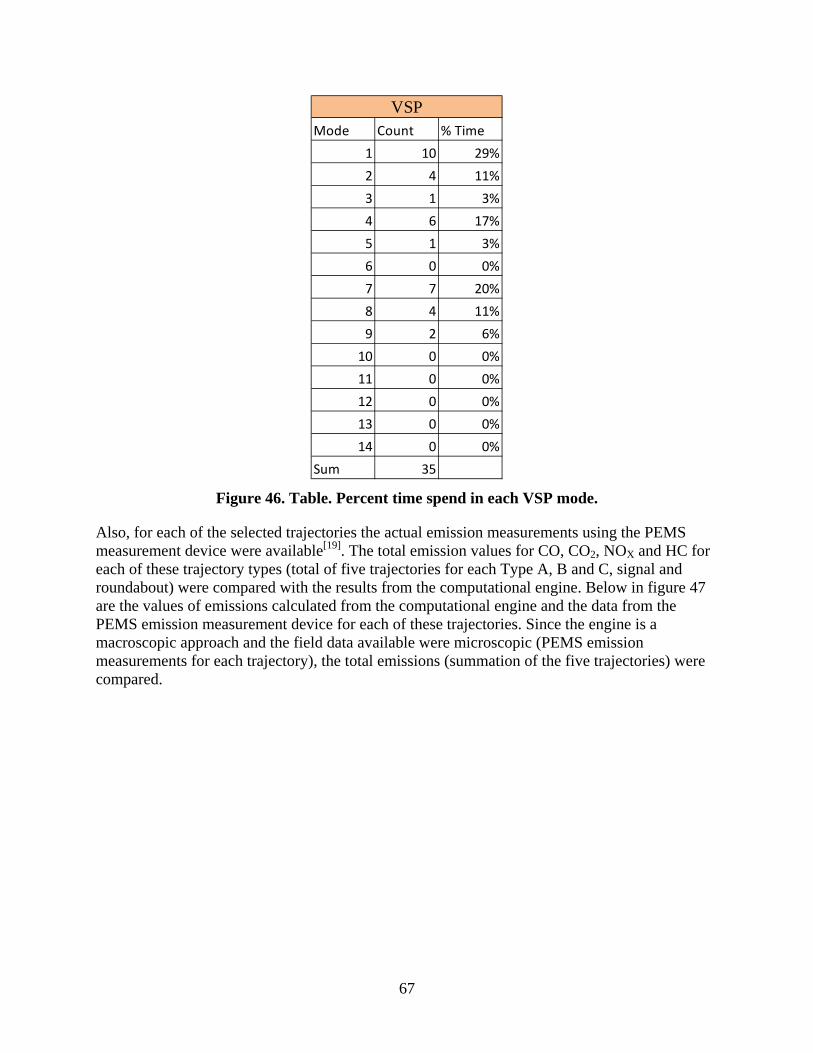
67

Figure 46. Table. Percent time spend in each VSP mode.

Also, for each of the selected trajectories the actual emission measurements using the PEMS measurement device were available[19]. The total emission values for CO, CO2, NOX and HC for each of these trajectory types (total of five trajectories for each Type A, B and C, signal and roundabout) were compared with the results from the computational engine. Below in figure 47 are the values of emissions calculated from the computational engine and the data from the PEMS emission measurement device for each of these trajectories. Since the engine is a macroscopic approach and the field data available were microscopic (PEMS emission measurements for each trajectory), the total emissions (summation of the five trajectories) were compared.

Mode Count % Time 1 10 29%2 4 11%3 1 3%4 6 17%5 1 3%6 0 0%7 7 20%8 4 11%9 2 6%

10 0 0%11 0 0%12 0 0%13 0 0%14 0 0%

Sum 35

VSP

68

Figure 47. Table. Validation results for 30 trajectories (15 low speed signal and 15 low

speed roundabout).

*The total seconds in each trajectory type was used to calculate the percent time spent in each VSP mode for each trajectory type and then calculate the total emissions results from the computational engine.

Trajectory Type Total seconds

Total Emission Values Over 5 TrajectoriesCO2 (g/sec.) CO (mg/sec) NOx (mg/sec) HC (mg/sec.)

Low Speed

Roundab

A 221 448.235 0.533 0.033 0.095B 613 865.982 0.974 0.068 0.186C 1217 2034.983 2.307 0.152 0.438

Low Speed Signal

A 197 277.025 0.316 0.022 0.059B 726 1197.904 1.242 0.082 0.259C 1581 2772.035 3.110 0.217 0.592

Computational Engine Output*Trajectory Type Total Seconds CO2 (g/sec.) CO (mg/sec) NOx (mg/sec) HC (mg/sec.)Low

Speed Roundab

A 221 483.729 0.564 0.039 0.104B 613 772.937 0.908 0.066 0.167C 1217 2215.774 2.117 0.143 0.470

Low Speed Signal

A 197 293.114 0.379 0.020 0.061B 726 1328.948 1.139 0.075 0.203C 1581 2702.025 3.707 0.260 0.520

69

REFERENCES

1. Coelho, M. C., Farias, T. L., & Rouphail, N. M. (2006). Effect of roundabout operations on pollutant emissions. Transportation Research Part D: Transport and Environment, 11 (5), 333-343.

2. Frey, H. C., Unal, A., Rouphail, N. M., & Colyar, J. D. (2003). On-road measurement of vehicle tailpipe emissions using a portable instrument. Journal of Air & Waste Manage. Assoc., 53(8), 992-1002.

3. Frey, H. C., Zhang, K., & Rouphail, N. M. (2008). Fuel use and emissions comparisons for alternative routes, time of day, road grade, and vehicles based on in-use measurements. Environmental Science and Technology, 42(7), 2483-2489.

4. U.S. EPA. (2010). MOVES1020 Highway Vehicle, Population and Activity Data, EPA-420-R-10-026. Ann Arbor, MI: U.S. Environmental Protection Agency.

5. Frey, H. C., Unal, A. Chen, J., Li, S., & Xuan, C. (2002). Methodology for developing modal emission rates for EPA's multi-scale motor vehicle and equipment emission estimation system (EPA Publication No. EPA420-R-02-027). Ann Arbor, MI: North Carolina State University for the U.S. Environmental Protection Agency.

6. Frey, H. C., Zhang, K. & Rouphail, N. M. (2010). Vehicle-specific emissions modeling based upon on-road measurements. Environmental Science and Technology, 44(9), 3594-3600.

7. Jimenez-Palacios, J. L. (1999). Understanding and quantifying motor vehicle emissions with vehicle specific power and TILDAS remote sensing (Doctoral dissertation). Department of Chemical Engineering, Massachusetts Institute of Technology, Cambridge, MA.

8. Hallmark, S., Fitzsimmons, E., Isebrands, H., & Giese, K. (2010). Roundabouts in signalized corridors. Transportation Research Record: Journal of the Transportation Research Board, 2182, 139-147. doi:10.3141/2182-18

9. Hallmark, S., Wang, B., Mudgal, A., & Isebrands, H. (2011). On-road evaluation of emission impacts of roundabouts. Transportation Research Record: Journal of the Transportation Research Board, 2265, 226-233. doi:10.3141/2265-25

10. Krogscheepers, J., & Watters, M. (2014). Roundabouts along rural arterials in South Africa. Paper presented at the Transportation Research Board 93nd Annual Meeting, Washington, DC.

70

11. Anya, A. R., Rouphail, N. M., Frey, H. C., & Liu, B. (2013). Method and case study for quantifying local emissions impacts of transportation improvement project involving road realignment and conversion to multilane roundabout. Transportation Research Records 2014, In Press.

12. Mudgal, A., Hallmark, S., Carriquiry, A., & Gkritza, K. (2014). Driving behavior at a roundabout: A hierarchical Bayesian regression analysis. Transportation Research Part D: Transport and Environment, 26(0), 20-26.

13. Ahn, K., Kronprasert, N., & Rakha, H. (2009). Energy and Environmental Assessment of High-Speed Roundabouts. Transportation Research Record: Journal of the Transportation Research Board, 2123, 54-65. doi:10.3141/2123-07

14. Chamberlin, R., Swanson, B., & Talbot, E. (2011). Analysis of MOVES and CNEM for evaluating the emissions impact of an intersection control change. Paper presented at the Transportation Research Board 90th Annual Meeting, Washington, DC.

15. Mandavilli, S., Rys, M.J., & Russell, E.R. (2008). Environmental impact of modern roundabouts. International Journal of Industrial Ergonomics, 38(2), pp.135-142.

16. Stevanovic, A., Stevanovic, J., Zhang, K., & Batterman, S. (2009). Optimizing traffic control to reduce fuel consumption and vehicular emissions: Integrated approach with VISSIM, CMEM, and VISGAOST. Transportation Research Record: Journal of the Transportation Research Board, 2128, 105-113.

17. Al-Ghandour, M. (2014). Analysis of fuel consumption and emissions at roundabout with slip lane, using SIDRA and validation by MOVES simulation. Proceedings from Second Transportation & Development Congress 2014, American Society of Civil Engineers, 2014, 300-310.

18. Song, G., Lei, Y., & Zhang, Y. (2012). Applicability of traffic microsimulation models in vehicle emissions estimates: Case study of VISSIM. Transportation Research Record: Journal of the Transportation Research Board, 2270, 132-141.

19. Frey, H. C., Yazdani-Boroujeni, B., Liu, B., Hu, J., & Jiao, W. (2013). Field measurements of 1996 to 2013 model year light duty gasoline vehicles. Proceedings from 106th Annual Conference, Air & Waste Management Association, Chicago, IL, June 25-28, 2013.

20. Salamati, K., Coelho, M. C., Fernandes, P. J., Rouphail. N. M., Frey, H. C., & Bandeira, J. (2013). Emission estimation at multilane roundabouts: Effect of movement and approach lane. Paper presented at the Transportation Research Board 92nd Annual Meeting, Washington, DC.

71

21. Transportation Research Board. (2010). Highway Capacity Manual. Washington, D.C.

22. PTV America. (n.d.). PTV Group. Retrieved from http://company.ptvgroup.com. Accessed July, 2014.

23. Yazdani, B., & Frey, H. C. Road grade quantification based on Global Positioning System data obtained from real-world vehicle fuel use and emission measurements. (2014). Atmospheric Environment, 85,179-186. http://dx.doi.org/10.1016/j.atmosenv.2013.12.025

24. U.S. EPA. (2012). Tier 0, Tier 1, and national low emission vehicle implementation schedule. Ann Arbor, MI: U.S. Environmental Protection Agency. Available from http://www.epa.gov/otaq/standards/light-duty/tiers0-1-schedule.htm

25. U.S. EPA. (2012) Tier 2 exhaust emission standards and implementation schedule. Ann Arbor, MI: U.S. Environmental Protection Agency. Available from http://www.epa.gov/otaq/standards/light-duty/tier2stds.htm

26. Ahn, K. (1998). Microscopic fuel consumption and emission modeling (Master’s thesis). Virginia Polytechnic Institute and State University, Blacksburg, VA.

27. Transport Simulation Systems. (2012). AIMSUN 7 Dynamic Simulators User's Manual. Barcelona, Spain: Transport Simulation Systems.

28. National Research Council. (2000). Modeling Mobile Source Emissions. Washington, D.C.: National Academy Press.

29. Kun, C., & Lei, Y. (2007). Microscopic traffic-emission simulation and case study for evaluation of traffic control strategies. Journal of Transportation Systems Engineering and Information Technology, 7(1), 93.

30. Smit, R., Ntziachristos, L., & Boulter, P. (2010). Validation of road vehicle and traffic emission models–A review and meta-analysis. Atmospheric Environment, 44(25), 2943-2953.

31. Nam, E. K., Gierczak, C. A., & Butler, J. W. (2003). A comparison of real-world and modelled emissions under conditions of variable driver aggressiveness. Paper presented at the 82nd Annual Meeting of the Transportation Research Board, Washington, DC.

32. Stathopoulos, F. G., & Noland, R.B. (2003). Induced travel and emissions from traffic flow improvement projects. Transportation Research Record: Journal of the Transportation Research Board, 1842, 57-63.

72

33. Jost, P., Hassel, D., Weber, F. J., & Sonnborn, K.S. (1992). Emission and fuel consumption modelling based on continuous measurements (No. DRIVE project V 1053). TUV Rheinland.

34. Park, J. Y., Noland, R. B., & Polak, J. W. (2001). Microscopic model of air pollutant concentrations: Comparison of simulated results with measured and macroscopic estimates. Transportation Research Record: Journal of the Transportation Research Board, 1750, 64-73.

35. Li, M., Boriboonsomsin, K., Wu, G., Zhang, W., & Barth, M. (2009). Traffic energy and emission reductions at signalized intersections: A study of the benefits of advanced driver information. International Journal of ITS Research, 7(1), 49-58.

36. Servin, O., Boriboonsomsin, K., & Barth, M. (2006, September). An energy and emissions impact evaluation of intelligent speed adaptation. In Intelligent Transportation Systems Conference, 2006. ITSC'06. IEEE (pp. 1257-1262). IEEE.

37. Boriboonsomsin, K., & Barth, M. (2008). Impacts of freeway high-occupancy vehicle lane configuration on vehicle emissions. Transportation Research Part D: Transport and Environment, 13(2), 112-125.

38. Barth, M., Malcom, C., & Scora, G. (2001). Integrating a comprehensive modal emissions model into ATMIS transportation modeling frameworks (California PATH Research Report No. UCB-ITS-PRR-2001-19). Berkeley, CA: California Path Program.

39. Qu, T., Rilett, L., & Zietsman, J. (2003). Estimating the impact of freeway speed limits on automobile emissions. Paper presented at the 82nd Annual Meeting of Transportation Research Board, Washington DC.

40. Franco, V., Kousoulidou, M., Muntean, M., Ntziachristos, L., Hausberger, S., & Dilara, P. (2013). Road vehicle emission factors development: A review. Atmospheric Environment, 70, 84-97.

41. Frey, H. C., Rouphail, N. M., & Zhai, H. (2006). Speed-and facility-specific emission estimates for on-road light-duty vehicles on the basis of real-world speed profiles. Transportation Research Record: Journal of the Transportation Research Board, 1987, 128-137.

42. Clean Air Technologies International (CATI). (2003). OEM-2100 Montana System Operational Manual. Buffalo, NY.

43. Sandhu, G. (2010). Methods for quality assurance of portable emissions measurement system data and methods for field comparison of alternative fuels (Master’s thesis). North Carolina State University, Raleigh, NC.

73

44. National Research Council. (2000). Modeling mobile source emissions. Washington, D.C.: National Academy Press.

45. North Carolina State University. (2002). Methodology for developing modal emission rates for EPA’s multi-scale motor vehicle and equipment emission system (EPA Publication No. EPA 420-R-02-027). Washington, DC: U.S. EPA.

46. Koupal, J., Landman, L., Nam, E. K., Warila, J., & Scarbro, C. (2005). MOVES2004 energy and emissions inputs draft report (U.S. EPA Publication No. EPA420-P-05-003). Washington, DC: U.S. EPA.

47. Wang, J., Yu, L., & Qiao, F. (2013). Micro traffic simulation approach to the evaluation of vehicle emissions on one‐way vs. two‐way streets: A case study in Houston downtown. Proceedings of the Transportation Research Board (TRB) 2013 Annual Meeting, Washington, DC.

48. Zhai, H. (2007). Regional on-road mobile source emissions characterization for conventional and Alternative vehicle technologies. (Ph.D, North Carolina State University).

49. Zhang, Y., Chen, X., Xiao, Z., Song, G., Yanzhao, H., & Lei, Y. (2009). Assessing effect of traffic signal control strategies on vehicle emissions. Journal of Transportation Systems Engineering and Information Technology, 9(1), 150-155.

50. Swidan, H. (2011). Integrating AIMSUN micro simulation model with portable emissions measurement system (PEMS): Calibration and validation case study (Masters Thesis). North Carolina State University, Raleigh, NC.

51. Song, G., Yu, L., & Xu, L. (2013). Comparative analysis of car-following models for emission estimation. Transportation Research Record: Journal of the Transportation Research Board, 2341, 12-22.

52. Panis, L., Broekx, S., & Liu, R. (2006). Modeling instantaneous traffic emissions and the influence of traffic speed limits. Science of the Total Environment, 371, 270-285.

53. Olstam, J. J., & Tapani, A. (2004). Comparison of car-following models (Publication No. VTI meddelande 960A). Linköping, Sweden: Swedish National Road Administration.

PUBLICATION NO. FHWA-SA-15-071