ACC1012 / ACC1053 Professional Skills / Introductory

ACC1012 / ACC1053

Professional Skills /

Introductory Quantitative Methods

Mathematics and Statistics

Semesters 1 & 2, 2017—2018

Lecturers: Dr. James Waldron & Dr. Kevin Wilson

School of Mathematics, Statistics & Physics

ii

☛

✡

✟

✠ACC1012/ACC1053

Professional Skills/Introductory Quantitative Methods

Lecturers: Dr. James Waldron & Dr. Kevin Wilson

Office: Room 2.14 (JW) & Room 2.19 (KW), Herschel Building

Email: [email protected]; [email protected]

Please see slides from the induction lecture for more detailed information on the course

organisation, including information on computer based assessments and case studies

Classes

• There will be one lecture every week: Friday 9:30–10:30 in 1.03 in NewcastleBusiness School.

• Each student will attend one of 8 scheduled workshops :

Group Day Time PlaceA Mon 12–1 Barbara Strang Teaching Centre 2.51B Mon 1–2 Barbara Strang Teaching Centre 2.51C Mon 4–5 Barbara Strang Teaching Centre 2.41BD Mon 5–6 Herschel Building TR1 (4th floor)E Tues 9–10 Barbara Strang Teaching Centre 3.31F Tues 12–1 Barbara Strang Teaching Centre 2.51G Tues 2–3 Barbara Strang Teaching Centre 2.51H Thurs 4–5 Barbara Strang Teaching Centre 3.31

Assessment

• 30% Professional Skills (see other sessions)

• 70% Mathematics & Statistics, consisting of:

– Written Maths & Stats exam at the end of the academic year (50%)

– Maths & Stats coursework, consisting of Computer Based Assessments(CBAs) and short written assignments based on case study material (20%)

The written exam will take place in May/June 2018; coursework will be set everyfew weeks, according to lecture material.

iii

Semester 1 deadlines

Assessment DeadlineCBA Practice mode opens Thursday 5th October

Assessed mode opens Thursday 12th OctoberDeadline: 23:59 Wednesday 18th October

Case Study Start work in tutorials w/b Monday 9th OctoberDeadline: 4pm, Friday 3rd November

Case Study Start work in tutorials w/b Monday 20th NovemberDeadline: 4pm, Friday 12th January

CBA Practice mode opens Thursday 30th NovemberAssessed mode opens Thursday 7th DecemberDeadline: 23:59 Wednesday 13th December

Deadlines for work in semester 2 will be announced in January

Other stuff

• Notes (with gaps) will be handed out in lectures – you should fill in the gapsduring lectures.

• A summarised version of the notes will be used in lectures as slides.

• These notes and slides will be posted on the course website after each topic isfinished, along with any other course material.

• The course website can be found via the “Additional teaching information” linkon the Maths & Stats webpage, in the ACC1012/ACC1053 Blackboard page, ordirectly via:

http://www.mas.ncl.ac.uk/∼nlf8/teaching/acc1012

• Please check your University email account regularly, as course announcementswill often be made via email.

• There is a course textbook available to buy at Blackwell’s – not compulsory, butwill be a good help!

• Calculators: the University has an approved list, available at

http://www.ncl.ac.uk/students/progress/exams/exams/CalculatorPolicy.htm

Chapter 1

Linear and quadratic functions

Before we start the main topics of the Mathematics & Statistics element of the module,we will spend some time reviewing linear and quadratic functions. To some extent, youhave already done this in the summer revision booklet. Nonetheless, it is importantthat you have completely mastered the basics before we move onto more challengingmaterial; the aim of the first chapter, then, is to quickly cover some old ground, and wewill do this through several examples.

1.1 Linear functions

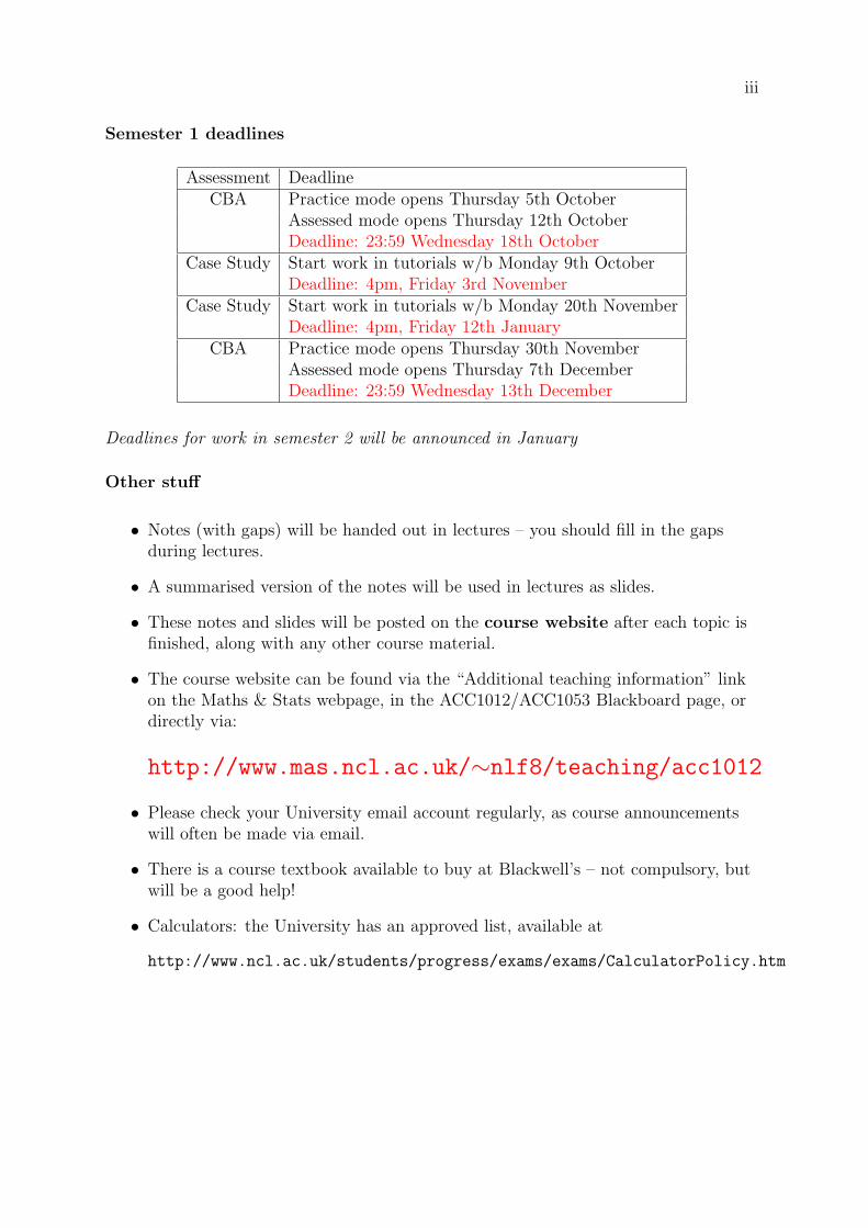
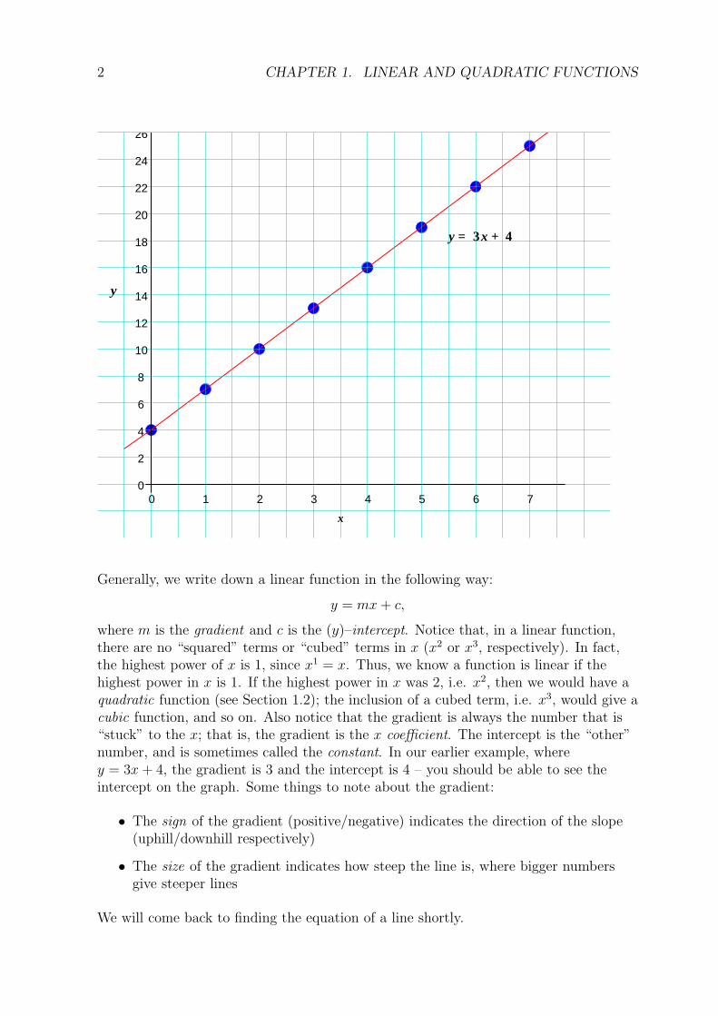
Linear functions occur often in accounting and finance. For example,

y = 3x+ 4

is a linear function. We know this is a linear function because when we produce agraph of the function, we get a straight line. For example, we can calculate the value ofy for various values of x by substitution (see Section 1.1.5 of the summer revisionbooklet); for instance, when x = 2, we get

y = 3× 2 + 4 = 6 + 4 = 10,

bearing in mind the rules of bidmas (see Section 1.1.1 of the summer revision booklet).Similarly, for other values of x, we can obtain the following table of results:

x 0 1 2 3 4 5 6 7y 4 7 10 13 16 19 22 25

Plotting x against y and joining up the points gives the graph shown overleaf. Noticethat we get a straight line – and so we could have produced exactly the same graphusing just two points instead of the eight we considered here (you only need two pointsto draw a straight line!).

1

2 CHAPTER 1. LINEAR AND QUADRATIC FUNCTIONS

2

4

6

8

10

12

14

16

18

20

22

24

26

00 1 2 3 4 5 6 7

x

y = 3x + 4

y

Generally, we write down a linear function in the following way:

y = mx+ c,

where m is the gradient and c is the (y)–intercept. Notice that, in a linear function,there are no “squared” terms or “cubed” terms in x (x2 or x3, respectively). In fact,the highest power of x is 1, since x1 = x. Thus, we know a function is linear if thehighest power in x is 1. If the highest power in x was 2, i.e. x2, then we would have aquadratic function (see Section 1.2); the inclusion of a cubed term, i.e. x3, would give acubic function, and so on. Also notice that the gradient is always the number that is“stuck” to the x; that is, the gradient is the x coefficient. The intercept is the “other”number, and is sometimes called the constant. In our earlier example, wherey = 3x+ 4, the gradient is 3 and the intercept is 4 – you should be able to see theintercept on the graph. Some things to note about the gradient:

• The sign of the gradient (positive/negative) indicates the direction of the slope(uphill/downhill respectively)

• The size of the gradient indicates how steep the line is, where bigger numbersgive steeper lines

We will come back to finding the equation of a line shortly.

1.1. LINEAR FUNCTIONS 3

1.1.1 Solving linear equations

In the summer revision booklet (Section 1.2.4), you should have thought about how tosolve simple linear equations. Let’s consider some more complicated examples. Don’tforget to bear in mind the rules about dealing with negatives! (see Section 1.1.2 of thesummer revision booklet).

Solve each of the following linear equations for x and t respectively.

1.6

x+ 4= 4;

2.−4t+ 4

5t− 6= −8.

✎


1.1.2 Finding the equation of a line

See Sections 1.2.3 and 1.2.5 of the summer revision booklet for more details.

Suppose we are told that the gradient of a line is 6. We are also told that the line passesthrough the point (3, 25). What is the equation of this line?

✎

Suppose we are told that a line passes through the points (1, 3) and (5, 35). What is theequation of the line?

✎


☛

✡

✟

✠Example 1.1The United Nations believes the annual consumption of rice in India (y kilograms perhousehold) is a linear function of the unit cost (x US $). They also know that, when theunit cost of rice is $12, the annual consumption of rice is 40.8kg per household; when thisunit cost doubles, the corresponding consumption decreases to 21.6kg per household.

(a) Using this information, obtain the linear function for demand in terms of cost.

(b) Find the unit cost of rice if the demand is 25kg per household.

✎


1.1.3 Solving two linear equations simultaneously

In real–life accounting and finance problems, we often have more than one equation tosolve. You might remember how to solve a pair of linear equations simultaneously fromyour GCSE maths course. If not, please see Section 1.2.6 of the summer revisionbooklet for more details, including how to solve a pair of simultaneous equationsgraphically.

Solve the following linear equations simultaneously; do not use a graph.

4x+ 8y = 30

7x− 6y = 5.

✎


☛

✡

✟

✠Example 1.2A cookie company makes two types of biscuit: standard and deluxe. Suppose the companymakes x batches of standard biscuits and y batches of deluxe biscuits every day.

(a) Each batch of standard biscuits requires 5kg of flour; each batch of deluxe biscuitsrequires 8kg of flour. Every day, exactly 98kg of flour must be used. Write down alinear equation in x and y for the total amount of flour used each day (in kg).

(b) Each batch of standard biscuits requires 2kg of butter; each batch of deluxe biscuitsrequires twice as much butter. Every day, exactly 44 kg of butter must be used.Write down a linear equation in x and y for the total amount of butter used eachday (in kg).

(c) Solve your equations in parts (a) and (b) simultaneously to find out how manybatches of standard and deluxe biscuits the company should make each day.

✎


1.1.4 Linear programming

Dynamic programming techniques were developed during the Second World War by agroup of American mathematicians. They sought to produce mathematical models ofsituations in which all the requirements, constraints and objectives were expressed asalgebraic equations. They then developed methods for obtaining the optimal solution –the maximum or minimum value of a required function.

In this section, we will attempt to formulate the requirements, constraints andobjectives of real–life accounting and finance problems as linear equations (after all,this chapter is all about linear functions!); this branch of dynamic programming isreferred to as linear programming, for obvious reasons. Thus, all algebraic expressionswill be of the form

(a number)x+ (a number)y;

for example,

Profit = 4x− 3y

is a linear equation for profit in terms of x and y, where x might represent ourexpenditure on advertising and y might be our costs.

Linear programming methods are some of the most widely used methods employed tosolve management and economic problems. They have been applied in a variety ofcontexts, some of which will be discussed in this chapter, with enormous savings inmoney and resources.

The first step is to formulate a problem as a linear programming problem; the secondstep is to solve the problem. In fact, much of the work we do here will rely on our workon simultaneous equations in the previous section, as well as our earlier graph work;however, there will be an emphasis on being able to construct the equations in the firstplace (as we did in Example 1.1), not just solving the equations, and this might take alittle time to master. In this section, we also need to think about linear inequalities ; forexample,

16x+ 18y ≤ 25

is a linear inequality in x and y. The role of inequalities will become apparent as wework through some examples.

Formulating linear programming problems

The first step in formulating a linear programming problem is to determine whichquantities you need to know to solve the problem. These are called the decision

variables.

The second step is to decide what the constraints are in the problem. For example,there may be a limit on resources or a maximum or minimum value a decision variablemay take, or there could be a relationship between two decision variables.


The third step is to determine the objective to be achieved. This is the quantity to bemaximised or minimised, that is, optimised. The function of the decision variables thatis to be optimised is called the objective function.

The examples which follow illustrate the varied nature of problems that can bemodelled by a linear programming model. We will not, at this stage, attempt to solvethese problems but instead concentrate on producing the objective function and theconstraints, writing these in terms of the decision variables.

☛

✡

✟

✠Example 1.3

A manufacturer makes two kinds of chairs, A and B, each of which has to be processedin two departments, I and II. Chair A has to be processed in department I for 3 hoursand in department II for 2 hours. Chair B has to be processed in department I for 3hours and in department II for 4 hours.

The time available in department I in any given month is 120 hours, and the timeavailable in department II, in the same month, is 150 hours.

Chair A has a selling price of £10 and chair B has a selling price of £12.

The manufacturer wishes to maximise his income. How many of each chair should bemade in order to achieve this objective? You may assume that all chairs made can besold.

At the minute, we will not attempt to solve this problem; we will simplyformulate the situation as a linear programming problem. You’ll notice that there’s alot of information given in the question – this is typical of a linear programmingproblem. Sometimes it’s easier to summarise the information given in a table:

Type of chair Time in dept. I (hours) Time in dept. II (hours) Selling price (£)

A 3 2 10B 3 4 12

Total time available 120 150

To formulate this linear programming problem, we consider the following three steps:

1. What are the decision variables? (i.e. which quantities do you need to know inorder to solve the problem?)

2. What are the constraints?

3. What is the objective?


Step 1: Decision variablesTo find out what the decision variables are, read through the question and identify thethings you’d like to know in order to solve the problem. You can usually do this bygoing straight to the last sentence of the question. The last sentence here is

“How many of each chair should be made...”

Thus, we’d like to know the number of type A chairs to make, and the number of typeB chairs to make. These are our decision variables, and are usually denoted with lowercase letters (x and y if we have two decision variables, x, y and z if we have three, forexample). Thus, our decision variables are

x = number of type A chairs made and

y = number of type B chairs made.

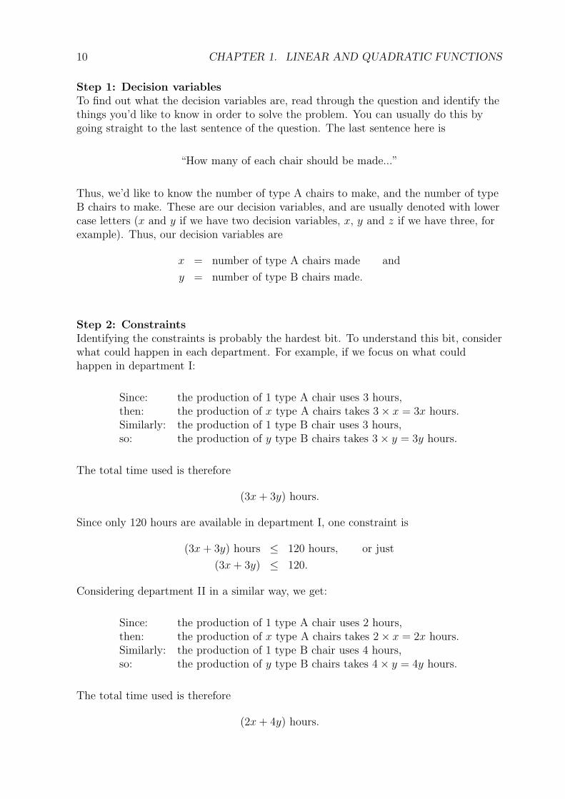
Step 2: ConstraintsIdentifying the constraints is probably the hardest bit. To understand this bit, considerwhat could happen in each department. For example, if we focus on what couldhappen in department I:

Since: the production of 1 type A chair uses 3 hours,then: the production of x type A chairs takes 3× x = 3x hours.Similarly: the production of 1 type B chair uses 3 hours,so: the production of y type B chairs takes 3× y = 3y hours.

The total time used is therefore

(3x+ 3y) hours.

Since only 120 hours are available in department I, one constraint is

(3x+ 3y) hours ≤ 120 hours, or just

(3x+ 3y) ≤ 120.

Considering department II in a similar way, we get:

Since: the production of 1 type A chair uses 2 hours,then: the production of x type A chairs takes 2× x = 2x hours.Similarly: the production of 1 type B chair uses 4 hours,so: the production of y type B chairs takes 4× y = 4y hours.

The total time used is therefore

(2x+ 4y) hours.


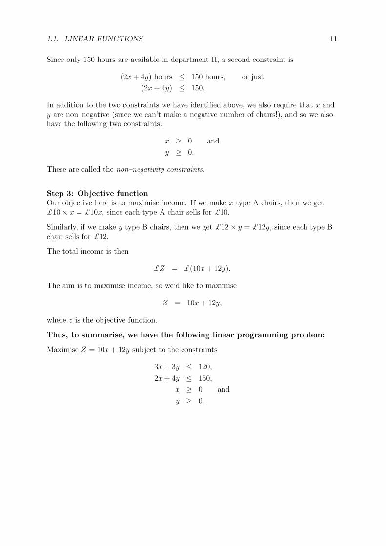
Since only 150 hours are available in department II, a second constraint is

(2x+ 4y) hours ≤ 150 hours, or just

(2x+ 4y) ≤ 150.

In addition to the two constraints we have identified above, we also require that x andy are non–negative (since we can’t make a negative number of chairs!), and so we alsohave the following two constraints:

x ≥ 0 and

y ≥ 0.

These are called the non–negativity constraints.

Step 3: Objective functionOur objective here is to maximise income. If we make x type A chairs, then we get£10× x = £10x, since each type A chair sells for £10.

Similarly, if we make y type B chairs, then we get £12× y = £12y, since each type Bchair sells for £12.

The total income is then

£Z = £(10x+ 12y).

The aim is to maximise income, so we’d like to maximise

Z = 10x+ 12y,

where z is the objective function.

Thus, to summarise, we have the following linear programming problem:

Maximise Z = 10x+ 12y subject to the constraints

3x+ 3y ≤ 120,

2x+ 4y ≤ 150,

x ≥ 0 and

y ≥ 0.


☛

✡

✟

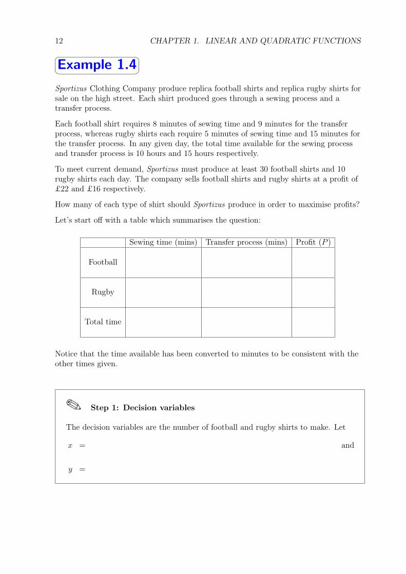
✠Example 1.4

Sportizus Clothing Company produce replica football shirts and replica rugby shirts forsale on the high street. Each shirt produced goes through a sewing process and atransfer process.

Each football shirt requires 8 minutes of sewing time and 9 minutes for the transferprocess, whereas rugby shirts each require 5 minutes of sewing time and 15 minutes forthe transfer process. In any given day, the total time available for the sewing processand transfer process is 10 hours and 15 hours respectively.

To meet current demand, Sportizus must produce at least 30 football shirts and 10rugby shirts each day. The company sells football shirts and rugby shirts at a profit of£22 and £16 respectively.

How many of each type of shirt should Sportizus produce in order to maximise profits?

Let’s start off with a table which summarises the question:

Sewing time (mins) Transfer process (mins) Profit (P )

Football

Rugby

Total time

Notice that the time available has been converted to minutes to be consistent with theother times given.

✎ Step 1: Decision variables

The decision variables are the number of football and rugby shirts to make. Let

x = number in paperback binding Lee Lee LeeLee Lee LeeLee Lee Lee and

y = number in library binding.


✎ Step 2: Constraints

The constraints are:

sewing : and

transfer :

We do, of course, also have the non–negativity conditions; however, we are also toldthat we must make at least 30 football shirts and 10 rugby shirts to meet demand,giving:

x ≥ and

y ≥

✎ Step 3: Objective function

✎ Thus, to summarise, we have:


Solving linear programming problems

We can attempt to solve the two linear programming problems in Examples 1.3 and 1.4graphically, using our earlier work on drawing graphs of linear functions. We do this byfinding the feasible region for the problem, and then finding the point within thisregion which optimises our objective function.

☛

✡

✟

✠Example 1.3 (revisited)

Recall that we had the following linear programming problem:

Maximise Z = 10x+ 12y subject to the following constraints:

3x+ 3y ≤ 120,

2x+ 4y ≤ 150,

x ≥ 0 and

y ≥ 0.

To find the feasible region for this problem (i.e. the region on a graph which satisfiesall of our inequalities), we proceed by indicating, on a diagram, the region for which allof the inequalities hold.

The first inequality is 3x+ 3y ≤ 120. To show this on a graph, we first need to plot theline 3x+ 3y = 120.

• When x = 0, we have

3× 0 + 3y = 120 i.e.

3y = 120 i.e.

y = 40.

• When y = 0, we have

3x+ 3× 0 = 120 i.e.

3x = 120 i.e.

x = 40.

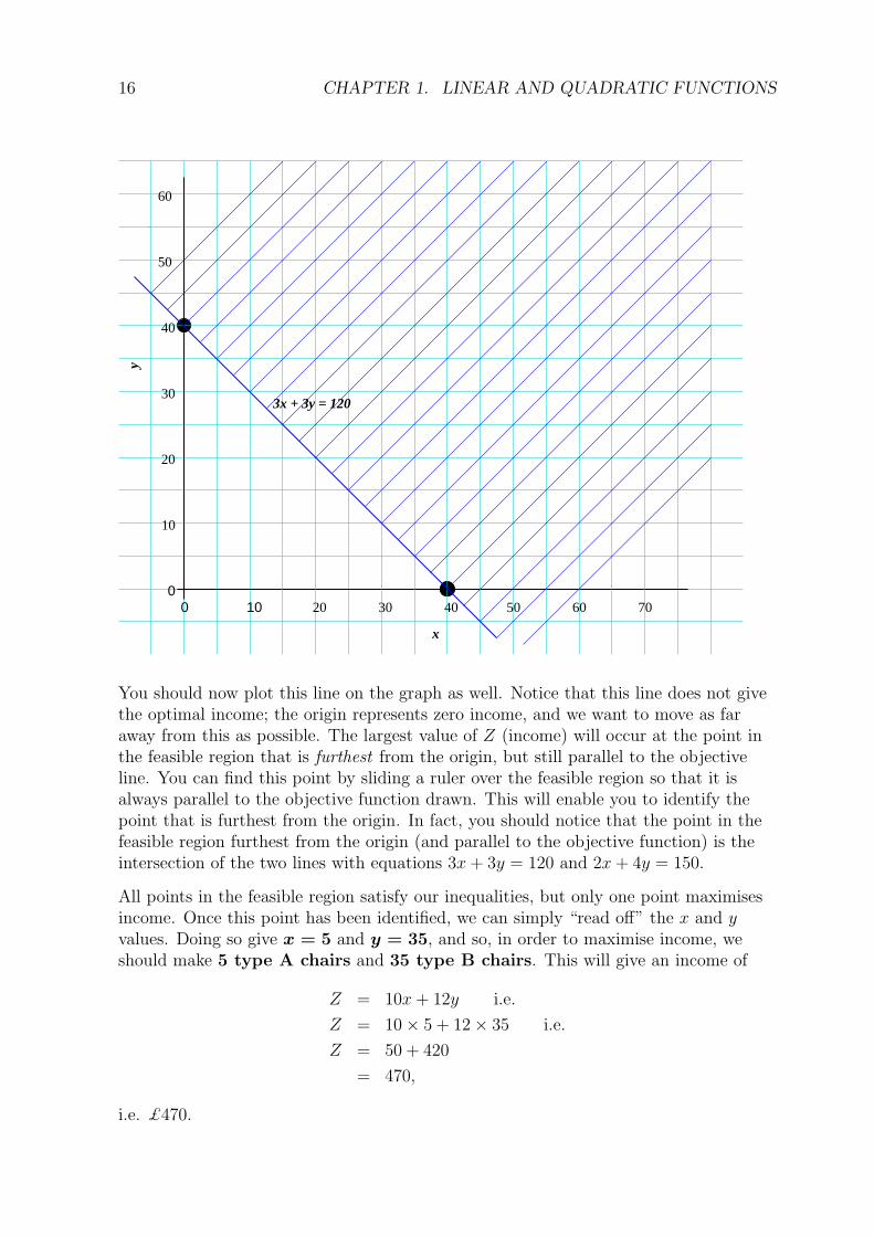
These points have been plotted on the graph overleaf and joined up to show the linewith equation 3x+ 3y = 120. Since we want 3x+ 3y ≤ 120, our region of interest lieson or below the line, and so we shade out the space above the line.


Now consider the second inequality 2x+ 4y ≤ 150. Again, to show this on a diagram,we first need to plot the line 2x+ 4y = 150.


2× 0 + 4y = 150 i.e.

4y = 150 i.e.

y = 37.5.


2x+ 4× 0 = 150 i.e.

2x = 150 i.e.

x = 75.

You should plot these points on the same graph overleaf, and hence draw the line withequation 2x+ 4y = 150. Since we want 2x+ 4y ≤ 150, our region of interest lies on orbelow the line, and so you should shade out the space above the line.

On the same graph we also shade out the inadmissible regions for the twonon–negativity constraints.

The unshaded region in the graph shows the feasible region associated with our set ofinequalities. What we must do now is find the point in that region which meets ourobjective – i.e. the point in that region which maximises income. One way of doingthis is to also plot the objective function. Now our objective function is

Z = 10x+ 12y,

where Z is our income. When Z takes different values we get a family of parallelstraight lines. We need to choose a starting value for Z in order to be able to plot theobjective function. It’s often a good idea to try a value which is a multiple of both thecoefficients of x and y. The coefficient of x is 10 and the coefficient of y is 12, so wecould try a starting value of Z = 120. Thus, the objective function is now

10x+ 12y = 120.

We can plot this line in the same way as before – i.e. consider what happens when x

and y are zero.


10× 0 + 12y = 120 i.e.

12y = 120 i.e.

y = 10.


10x+ 12× 0 = 120 i.e.

10x = 120 i.e.

x = 12.


0

0

x

y

10

20

30

40

10 20 30 40 50 60 70

60

50

3x + 3y = 120

You should now plot this line on the graph as well. Notice that this line does not givethe optimal income; the origin represents zero income, and we want to move as faraway from this as possible. The largest value of Z (income) will occur at the point inthe feasible region that is furthest from the origin, but still parallel to the objectiveline. You can find this point by sliding a ruler over the feasible region so that it isalways parallel to the objective function drawn. This will enable you to identify thepoint that is furthest from the origin. In fact, you should notice that the point in thefeasible region furthest from the origin (and parallel to the objective function) is theintersection of the two lines with equations 3x+ 3y = 120 and 2x+ 4y = 150.

All points in the feasible region satisfy our inequalities, but only one point maximisesincome. Once this point has been identified, we can simply “read off” the x and y

values. Doing so give x = 5 and y = 35, and so, in order to maximise income, weshould make 5 type A chairs and 35 type B chairs. This will give an income of

Z = 10x+ 12y i.e.

Z = 10× 5 + 12× 35 i.e.

Z = 50 + 420

= 470,

i.e. £470.


☛

✡

✟

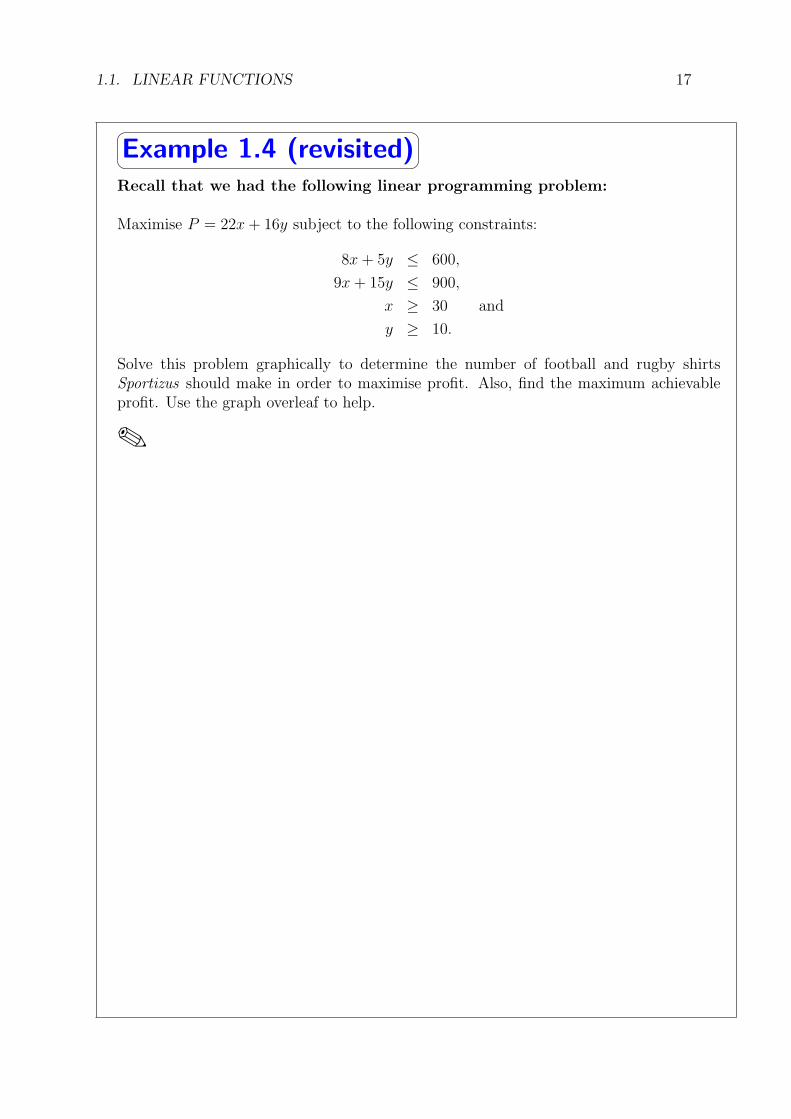
✠Example 1.4 (revisited)Recall that we had the following linear programming problem:

Maximise P = 22x+ 16y subject to the following constraints:

8x+ 5y ≤ 600,

9x+ 15y ≤ 900,

x ≥ 30 and

y ≥ 10.

Solve this problem graphically to determine the number of football and rugby shirtsSportizus should make in order to maximise profit. Also, find the maximum achievableprofit. Use the graph overleaf to help.

✎


0

0

x

y

20

40

60

80

100

120

20 40 60 80 100 120

Both of these problems can also be solved algebraically by solving the pair ofsimultaneous equations shown in both graphs – you should try this yourself based onthe material in Section 1.1.3.

1.2 Quadratic functions

As you might imagine, not everything in real–life can be represented by a straight lineand, at best, the linear functions we looked at in Section 1.1 – such as linear costfunctions and linear functions for profit – are simplifications. To this end, in thissection we will consider the role of non–linear functions in the field of accounting andfinance. In particular, we will think about polynomial functions where the power in x isgreater than 1 (giving a non–linear graph). The simplest case here is the quadratic

function, where the highest power of x in our polynomial is 2 – that is, at most we havean x2 term. For example,

y = 5x2 − 2x+ 6

is a quadratic, since the highest power of x is 2; the polynomial

y = 2x4 − 3x2 + 9

is not a quadratic, since the highest power of x here is 4 (in fact, this is a quartic).

1.2. QUADRATIC FUNCTIONS 19

1.2.1 Plotting quadratic functions

In the space below, plot the graph of the function y = x2 − 2x− 15.

✎

10

8

6

4

2

−2

−4

−6

−8

−10

−12

−14

−16

−1−2−3−4 1 2 3 4 x

y


☛

✡

✟

✠Example 1.5The estates manager of a zoo has 100 metres of fencing to construct a rectangular enclosurefor some West African camels.

(a) Formulate a non–linear function for the area of the enclosure in terms of its width,x metres.

(b) Produce a plot of your non–linear function in (a) (see overleaf).

(c) Using your plot in (b), what length x would give the optimal area for the camelenclosure? What area would this give?

✎


10 20 30 40 50 60

100

200

300

400

500

600

x

Area

As with linear functions, it would be useful to be able to plot or sketch a non–linearfunction without having to draw up a full table of results. For a quadratic function, itmight be useful to know where the curve cuts into the x–axis, as well as the y–interceptof the curve. Consider the quadratic from the earlier example: y = x2 − 2x− 15. Weknow the y–intercept occurs when x = 0, that is

y = 02 − 2× 0− 15 = −15,

and this can be seen in our plot of this function. However, how can we tell, withoutdrawing up a full table of results, where the curve will cut the x–axis? The curve cutsthe x–axis when y = 0, that is when

x2 − 2x− 15 = 0,

and so we would need to solve this equation for x. However, this is an example of aquadratic equation, and we haven’t considered how to solve these yet...


1.2.2 Solving quadratic equations

We can visualise the solution(s) for x in the equation

ax2 + bx+ c = 0

by looking at a plot of the quadratic and noting where the curve intersects/touches theline y = 0, that is, the x–axis. However, the accuracy of our solutions obtained in thisway will depend on the accuracy of our graph. We would also need to know what rangeof x–values to draw the graph over. Two approaches for solving quadratics a bit moremathematically will now be considered. In both, we will assume the general form of aquadratic as

y = ax2 + bx+ c;

the discriminant, D, is given byD = b2 − 4ac,

and has important properties in terms of how we classify the solutions to our quadratic.

Factorisation

If the discriminant is a perfect square – that is, if the square root of D as defined aboveis an integer value, then we can solve our quadratic by the method of factorisa-tion. For more help with this, see Sections 1.3.1 and 1.3.2 of the summer revision booklet.

Consider the following quadratic equations:

1. x2 − 2x− 15 = 0 (from earlier – see page 19)

2. x2 + 5x+ 2 = 0

3. x2 − 8x+ 12 = 0

4. x2 − 5x− 36 = 0

5. 2x2 − 7x+ 5 = 0

(a) For each, find the discriminant D.

✎


(b) Which equations can be solved by factorisation?

✎

(c) Solve the equations identified in (b) by factorisation.

✎


Quadratic formula

If we cannot factorise our quadratic, then we can use the quadratic formula in order tofind the solution(s) to our quadratic equation. For example, equation (2) in the lastquestion:

x2 + 5x+ 2 = 0

could not be factorised because the discriminant is

D = 52 − (4× 1× 2) = 25− 8 = 17,

which is not a perfect square. However, all is not lost: the quadratic formula can helpus here! This was developed by Indian mathematicians in around 628AD, although theformula as we know it today was not published until 1637 by a French mathematician.The solution(s) to the equation

ax2 + bx+ c = 0,

with discriminant D = b2 − 4ac, are given by the formula

x =−b±

√D

2a.

For example, consider the quadratic equation we plotted on page 19:

y = x2 − 2x− 15.

The graph showed that when y = 0 the solutions were x = 5 and x = −3. Earlier inthis section we also solved this equation by the method of factorisation. What aboutusing the formula?

Note that a = 1, b = −2 and c = −15. Thus the discriminant is

D = (−2)2 − 4× 1×−15 = 64.

So by the formula, we have

x =−(−2)±

√64

2× 1

=2± 8

2.

So the solutions are given by

x =2 + 8

2=

10

2= 5,

or

x =2− 8

2=

−6

3= −3,

exactly the solutions we obtained graphically and by factorisation!


Solve the quadratic equationx2 + 5x+ 2 = 0.

✎


☛

✡

✟

✠Example 1.6A company models its annual profits using the function

P (x) = x2 + 20x− 300,

where P represents profits and x is the number of units sold. In 2011 their profits were£167,700. How many units of their product did they sell?

✎


☛

✡

✟

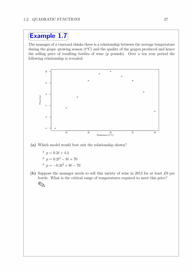
✠Example 1.7The manager of a vineyard thinks there is a relationship between the average temperatureduring the grape–growing season (toC) and the quality of the grapes produced and hencethe selling price of resulting bottles of wine (p pounds). Over a ten year period thefollowing relationship is revealed:

56

78

910

16 18 20 22 24

Temperature (toC)

Price

(£p)

(a) Which model would best suit the relationship shown?

* p = 0.2t+ 4.4

* p = 0.2t2 − 8t+ 70

* p = −0.2t2 + 8t− 70

(b) Suppose the manager needs to sell this variety of wine in 2013 for at least £9 perbottle. What is the critical range of temperatures required to meet this price?

✎


Summary

Earlier, we discussed that the discriminant D = b2 − 4ac has important properties interms of how we classify he solutions to our quadratic equation. In summary:

• If D is a perfect square, then we can solve the quadratic by factorisation;otherwise, we can use the formula (in fact, the formulae will always work!)

• If D > 0, our quadratic will have two real solutions – that is, the curve will cutthe x–axis in two places

• If D = 0, then our quadratic will have repeated solutions – that is, our graph onlyjust touches the x–axis (in effect giving just a single solution)

• If D < 0, then we cannot operate the quadratic formula as we cannot take thesquare root of a negative – at least, not in the real number system. Actually, sucha quadratic has complex roots making use of the complex number system, butthis goes beyond the scope of this module

1.3 Higher–order polynomials

In more complicated accounting and finance problems, linear and/or quadraticfunctions might still not be adequate enough to model our situation realistically.Higher–order polynomials can be used, such as cubics:

y = ax3 + bx2 + cx+ d,

or even quartics:y = ax4 + bx3 + cx2 + dx+ e;

or even quintics! –y = ax5 + bx4 + cx3 + dx2 + ex + f.

We will return to such functions in Chapter 2 of this course.

1.4. CHAPTER 1 PRACTICE QUESTIONS 29

1.4 Chapter 1 practice questions

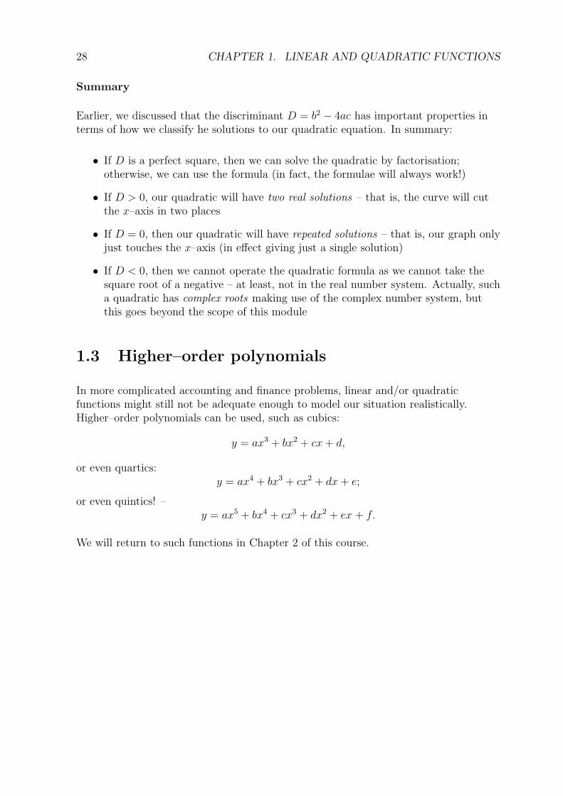
1. What are the intercept and gradient of the following linear functions?

(a) y = 2x+ 5

(b) y = 12− 2x

(c) 8y = 2x+ 16

(d) y = x

2. Put the linear functions in question 1 in order of “steepness”, from most steep toleast steep.

3. On the graph below, plot each of the linear functions given in question 1.

0

0

2 4 6 8 10 12 14

2

4

6

8

10

12

x

y


4. A recent British Gas investigation examined factors which influenced the lengthof time it takes customers to pay their utility bills (see the British Gas websitefor details about this investigation and a fully downloadable report). Their reportrevealed that the size of a customer’s bill (£x) was the most important factorinfluencing the time it took customers to pay this bill (y, in days).

In particular, British Gas express the time it takes a customer to pay their bill asa linear function of the size of their bill:

y = 0.06x+ 7.44.

(a) What are the intercept and gradient of this linear function?

(b) If Kristina Bell’s gas bill is £450, how long can we expect it will take her topay this bill?

(c) Suppose it took Maeve Campbell 10 days to pay her gas bill. Solve theabove linear equation for x to find out how Maeve’s gas bill was.

5. Jake Bennett needs a new carpet for his bedroom. His room is rectangular inshape, and the length of the room is 3 times the width. Let x be the width of theroom, in metres.

(a) Write down an expression for the perimeter of Jake’s bedroom. Simplify thisexpression as far as possible.

(b) Write down an expression for the area of Jake’s bedroom.

(c) Which one of your expressions in (a) and (b) is linear?

6. Alexander Booth is an entrepreneur who has recently developed a miraclehangover cure. The number of hours until a hangover is cured (y) is thought tobe related to the dose given (x mg).

Specifically, if a person suffering with a hangover is not given any of the drug atall, the hangover will pass within 10 hours. However, a 50mg dose should see thehangover pass within 2 hours.

(a) Assuming y is a linear function of x, find the intercept c and the gradient m,and hence write down the linear function.

(b) Assuming side effects are negligible regardless of the dose, what is theoptimal dose to give hangover sufferers?


7. Using a mobile phone costs £30 per month, and an additional 16 pence perminute of use (texts are free).

(a) Write down a linear function of cost in terms of minutes used each month.Make sure you clearly define any variables.

(b) Suppose you make 3.5 hours worth of calls this month. How much shouldyour bill be?

(c) You now upgrade your mobile phone. Under your new tariff you pay £25per month and only 5 pence per minute of use. Text messages are still free,but your new phone is a smart phone and you will be charged 50p pergigabyte of data you use. Write down a linear function for cost in terms ofcall time and data, clearly defining any variables.

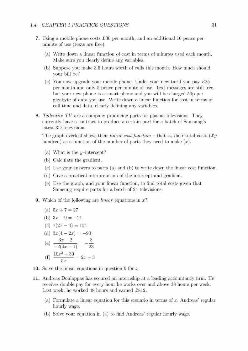
8. Tallentire TV are a company producing parts for plasma televisions. Theycurrently have a contract to produce a certain part for a batch of Samsung’slatest 3D televisions.

The graph overleaf shows their linear cost function – that is, their total costs (£yhundred) as a function of the number of parts they need to make (x).

(a) What is the y–intercept?

(b) Calculate the gradient.

(c) Use your answers to parts (a) and (b) to write down the linear cost function.

(d) Give a practical interpretation of the intercept and gradient.

(e) Use the graph, and your linear function, to find total costs given thatSamsung require parts for a batch of 24 televisions.

9. Which of the following are linear equations in x?

(a) 5x+ 7 = 27

(b) 3x− 9 = −21

(c) 7(2x− 4) = 154

(d) 3x(4− 2x) = −90

(e)3x− 2

−2(4x− 1)= −

8

23

(f)10x2 + 30

5x= 2x+ 3

10. Solve the linear equations in question 9 for x.

11. Andreas Doulappas has secured an internship at a leading accountancy firm. Hereceives double pay for every hour he works over and above 38 hours per week.Last week, he worked 48 hours and earned £812.

(a) Formulate a linear equation for this scenario in terms of x, Andreas’ regularhourly wage.

(b) Solve your equation in (a) to find Andreas’ regular hourly wage.


0

0

2

4

6

8

10

12

x

y

5 10 15 20 25 30 35

12. Wong Enterprises have a team of quantitative analysts who forecast the profitmargins of their clients. For one company, they show that profit is directlyrelated to total income and overheads, that is

Profit = total income− overheads,

where total income itself is a linear function of advertising expenditure (£x):

Total income = 6(x− 2000).

If the company’s profit last month was £188,000, and their overheads were£10,000, how much did they spend on advertising?

13. (a) The gradient of a straight line is −0.75. If the line passes through the point(−6, 1), find the equation of the line in the form y = mx+ c.

(b) Another straight line passes through the points (2, 11) and (5, 38). Find theequation of this line in the form y = mx+ c.


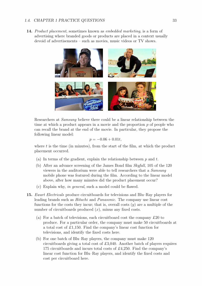
14. Product placement, sometimes known as embedded marketing, is a form ofadvertising where branded goods or products are placed in a context usuallydevoid of advertisements – such as movies, music videos or TV shows.

Researchers at Samsung believe there could be a linear relationship between thetime at which a product appears in a movie and the proportion p of people whocan recall the brand at the end of the movie. In particular, they propose thefollowing linear model:

p = −0.06 + 0.01t,

where t is the time (in minutes), from the start of the film, at which the productplacement occurred.

(a) In terms of the gradient, explain the relationship between p and t.

(b) After an advance screening of the James Bond film Skyfall, 105 of the 120viewers in the auditorium were able to tell researchers that a Samsung

mobile phone was featured during the film. According to the linear modelabove, after how many minutes did the product placement occur?

(c) Explain why, in general, such a model could be flawed.

15. Ewart Electricals produce circuitboards for televisions and Blu–Ray players forleading brands such as Hitachi and Panasonic. The company use linear costfunctions for the costs they incur; that is, overall costs (y) are a multiple of thenumber of circuitboards produced (x), minus any fixed costs.

(a) For a batch of televisions, each circuitboard cost the company £20 toproduce. For a particular order, the company must make 50 circuitboards ata total cost of £1,150. Find the company’s linear cost function fortelevisions, and identify the fixed costs here.

(b) For one batch of Blu–Ray players, the company must make 120circuitboards giving a total cost of £3,040. Another batch of players requires175 circuitboards and incurs total costs of £4,250. Find the company’slinear cost function for Blu–Ray players, and identify the fixed costs andcost per circuitboard here.


16. Solve the following pairs of linear equations simultaneously for (x, y), (p, q) or(A,B):

2x+ 3y = 18

2x+ y = 14

4x+ 5y = 65

3x− 3y = −12

6p+ 3q = 108

4p+ 7q = 122

6A+ 2B = 20 + 5B

5A+ 10B + 6 = 13B + 17

17. The Monster Party Company produce two types of party pack. Their “Ghastly”party pack contains 10 balloons and 64 sweets. Their “Devilish” party packcontains 20 balloons and 16 sweets. Each week, the company must use 3000balloons and 8000 sweets in their party packs.

(a) How many “Ghastly” and “Devilish” party packs can the company makeeach week? Solve this problem graphically and algebraically.

(b) The company sells each “Ghastly” party pack at a profit of £1.20 and each“Devilish” party pack at a profit of £1.80. How much profit can they expectto make each week?

18. Kuddly Pals Co. Ltd make two types of giant soft toy: bears and cats. Thequantity of material needed and the time taken to make each type of toy is givenin the table below.

Toy Material (m2) Time (minutes)Bear 5 12Cat 8 8

Each day the company can process up to 2000m2 of material and there are 48worker hours available to assemble the toys.

The profit made on each bear is £1.50 and on each cat is £1.75. Kuddly Pals Co.Ltd wishes to maximise its daily profit.

(a) Formulate the company’s situation as a linear programming problem.

(b) Draw a suitable diagram to enable the problem to be solved graphically,indicating the feasible region and the direction of the objective line.

(c) Use your diagram to find the company’s maximum profit, £P .

(d) Verify your solution algebraically.


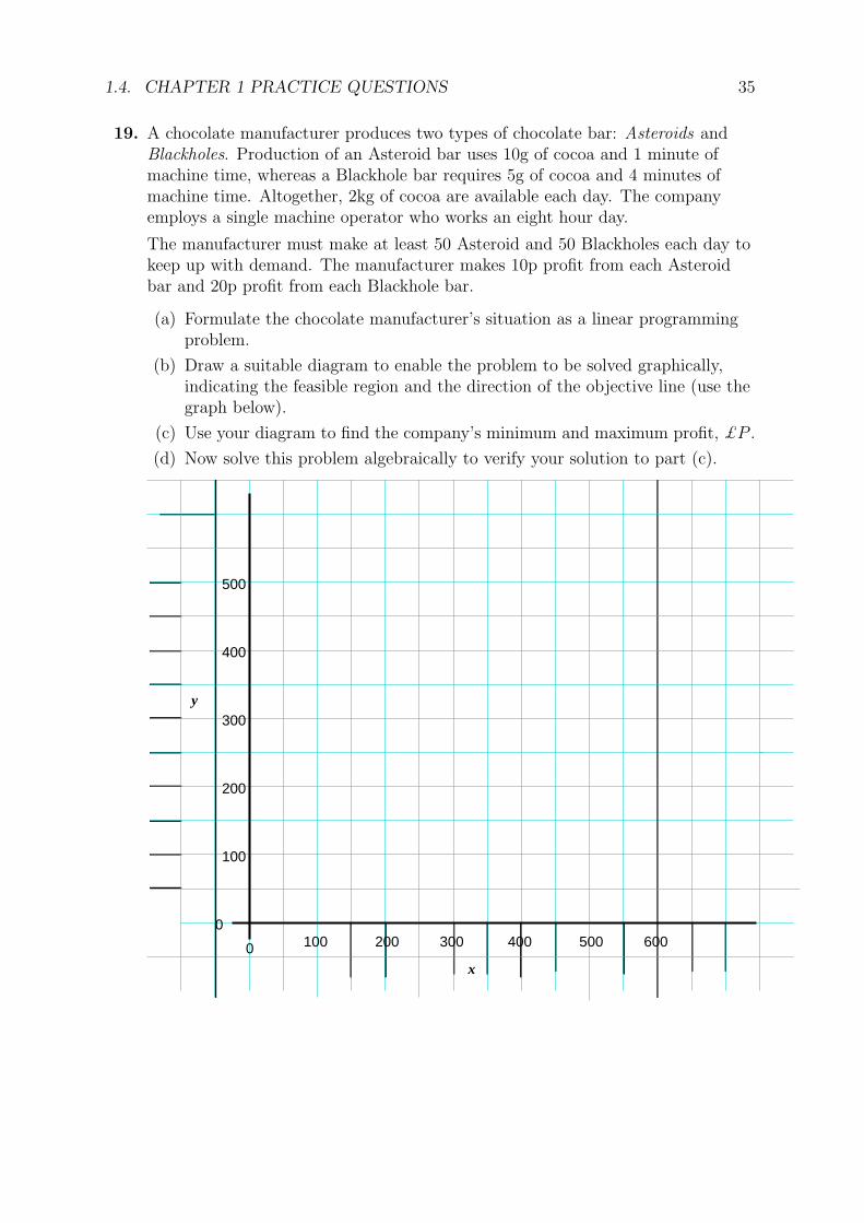
19. A chocolate manufacturer produces two types of chocolate bar: Asteroids andBlackholes. Production of an Asteroid bar uses 10g of cocoa and 1 minute ofmachine time, whereas a Blackhole bar requires 5g of cocoa and 4 minutes ofmachine time. Altogether, 2kg of cocoa are available each day. The companyemploys a single machine operator who works an eight hour day.

The manufacturer must make at least 50 Asteroid and 50 Blackholes each day tokeep up with demand. The manufacturer makes 10p profit from each Asteroidbar and 20p profit from each Blackhole bar.

(a) Formulate the chocolate manufacturer’s situation as a linear programmingproblem.

(b) Draw a suitable diagram to enable the problem to be solved graphically,indicating the feasible region and the direction of the objective line (use thegraph below).

(c) Use your diagram to find the company’s minimum and maximum profit, £P .

(d) Now solve this problem algebraically to verify your solution to part (c).

x

100 200 300 400 500 600

100

200

300

400

500

0

0

y


20. Which of the following are quadratic equations in x?

(i) 5x+ 9 = 2x− 3

(ii) x2 + 11x+ 28 = 0

(iii) x2 − 4x = 5

(iv) x2 + 3x+ 1 = 0

(v)6x2 + 5x+ 26

2x= 3x+ 4

(vi) x2 + 10 = 6x

(vii) x2 − 16x+ 64 = 0

21. For each of the quadratic equations in question 20, calculate the discriminant.Using this value,

(a) decide whether the quadratic will have two distinct solutions, repeatedsolutions or complex solutions;

(b) decide which could be solved using the method of factorisation.

22. (a) Solve the quadratic equations you have identified in question 21(b) using themethod of factorisation.

(b) For any remaining quadratics in question 20 that can be solved, use thequadratic formula to solve for x.

23. The amount of profit a company makes, £π million, is related to their advertisingexpenditure £q million according to the following function:

π(q) = −2q2 + 9q − 4.

Find the company’s break–even points, that is, their advertising expenditure thatgives zero profit. Also, produce a sketch of π(q).

24. In the 1950’s, the Japanese statistician Genichi Taguchi (1924–2012) developed atechnology for applying mathematics and statistics to improve the quality ofmanufactured goods. Taguchi quality loss functions are now used frequently inthe fields of accounting, finance, business and economics. In general, the Taguchiloss function is given by

L = k(x−m)2,

where

– L is the monetary loss

– x is the quality characteristic (e.g. concentration, diameter,...)

– m is the target value for x

– k is a constant


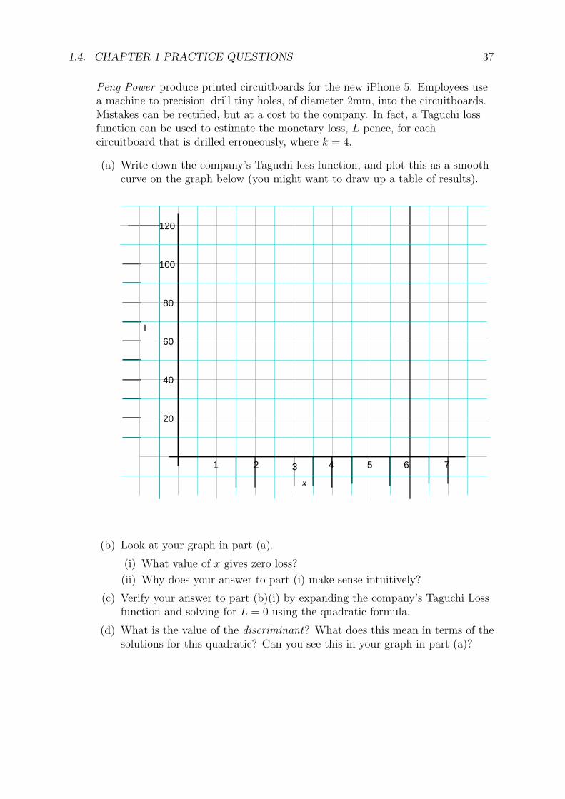
Peng Power produce printed circuitboards for the new iPhone 5. Employees usea machine to precision–drill tiny holes, of diameter 2mm, into the circuitboards.Mistakes can be rectified, but at a cost to the company. In fact, a Taguchi lossfunction can be used to estimate the monetary loss, L pence, for eachcircuitboard that is drilled erroneously, where k = 4.

(a) Write down the company’s Taguchi loss function, and plot this as a smoothcurve on the graph below (you might want to draw up a table of results).

1 2 3 4 5 6 7

20

40

60

80

100

120

x

L

(b) Look at your graph in part (a).

(i) What value of x gives zero loss?

(ii) Why does your answer to part (i) make sense intuitively?

(c) Verify your answer to part (b)(i) by expanding the company’s Taguchi Lossfunction and solving for L = 0 using the quadratic formula.

(d) What is the value of the discriminant? What does this mean in terms of thesolutions for this quadratic? Can you see this in your graph in part (a)?

Documents

ACC1012 / ACC1053 Professional Skills / Introductory