Embed Size (px)
Citation preview
Chapter 5
Continuous probability models
Dr. James Waldron, Dr. Lee Fawcett ACC1012 / 1053: Mathematics & Statistics
What we’ll cover...
Probability density functions
The Normal distribution
The Uniform distribution
The exponential distribution
Poisson processes
Dr. James Waldron, Dr. Lee Fawcett ACC1012 / 1053: Mathematics & Statistics
5. Continuous probability models
We have seen how discrete random variables can be modelledby discrete probability distributions such as the binomial andPoisson distributions.
We now consider how to model continuous random variables.
Dr. James Waldron, Dr. Lee Fawcett ACC1012 / 1053: Mathematics & Statistics
5.1 Introduction
A variable is discrete if it takes a countable number of values.
For example ,
– the number of blue cars that I count in a 5 minute period
– the number of heads observed when I flip a coin ten times
– Shoe sizes: 1, . . . ,12,13,1,2, . . .
– r = 0,0.1,0.2, . . . ,0.9,1.0
In contrast, the values which a continuous variable can takeform a continuous scale , with no “jumps”.
For example ,
– Height
– Weight
– Temperature
Dr. James Waldron, Dr. Lee Fawcett ACC1012 / 1053: Mathematics & Statistics
5.1 Introduction
Think about height .
In practice, we might only record height to the nearest cm
If we could measure height exactly we’d find that everyonehad a different height
This is the essential difference between discrete andcontinuous variables
If there are n people on the planet, the probability thatsomeone’s height is x would be 1
n
As n gets bigger and bigger, this probability tends to zero!!
Dr. James Waldron, Dr. Lee Fawcett ACC1012 / 1053: Mathematics & Statistics
5.1 Introduction
Consider taking a sample of values from:
X : Weight of 10oz burger.
Dr. James Waldron, Dr. Lee Fawcett ACC1012 / 1053: Mathematics & Statistics
5.1 Introduction
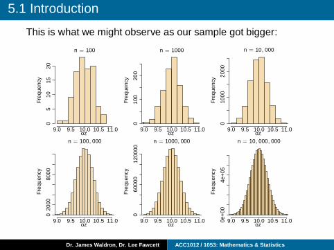
This is what we might observe as our sample got bigger:
Freq
uenc
y
Freq
uenc
y
Freq
uenc
y
Freq
uenc
y
Freq
uenc
y
Freq
uenc
y
ozozoz
ozozoz
n = 100 n = 1000 n = 10, 000
n = 100, 000 n = 1000, 000 n = 10, 000, 000
9.09.09.0
9.09.09.0
9.59.59.5
9.59.59.5
10.010.010.0
10.010.010.0
10.510.510.5
10.510.510.5
11.011.011.0
11.011.011.000
0005
1015
20
100
200
1000
2000
2000
8000
6000
012
0000
0e+
004e
+05
Dr. James Waldron, Dr. Lee Fawcett ACC1012 / 1053: Mathematics & Statistics
5.1 Introduction
As the sample size gets bigger, the interval widths getsmaller
the jagged profile of the histogram smooths out tobecome a curve
When the sample size is infinitely large, this curve isknown as the probability density function (pdf)
Dr. James Waldron, Dr. Lee Fawcett ACC1012 / 1053: Mathematics & Statistics
Features of the probability density function
The key features of pdfs are:
1 pdfs never take negative values
2 the area under a pdf is one: P(−∞ < X < ∞) = 1
3 areas under the curve correspond to probabilities
4 P(X ≤ x) = P(X < x) since P(X = x) = 0.
Dr. James Waldron, Dr. Lee Fawcett ACC1012 / 1053: Mathematics & Statistics
5.1 Introduction
Over the next two weeks we will consider some particularprobability distributions that are often used to describecontinuous random variables.
We start with the most important , most widely–used statisticaldistribution of all time...
...wait for it...
Dr. James Waldron, Dr. Lee Fawcett ACC1012 / 1053: Mathematics & Statistics
5.2 The Normal distribution
☛
✡
✟
✠The Normal Distribution
Dr. James Waldron, Dr. Lee Fawcett ACC1012 / 1053: Mathematics & Statistics
5.2.1 Introduction
The Normal distribution is without doubt the mostwidely–used statistical distribution in many practicalapplications:
Normality arises naturally in many physical, biological andsocial measurement situations
Normality is important in Statistical inferenceThe normal distribution has many guises:
– Gaussian distribution– Laplacean distribution– “bell–shaped curve”
Dr. James Waldron, Dr. Lee Fawcett ACC1012 / 1053: Mathematics & Statistics
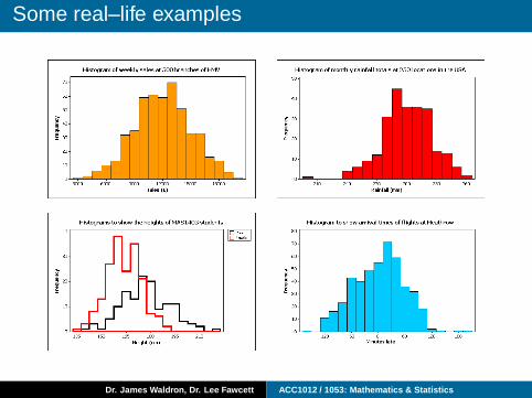
Some real–life examples
Dr. James Waldron, Dr. Lee Fawcett ACC1012 / 1053: Mathematics & Statistics
5.2.1 Introduction
Recall the “parameters” of the binomial and Poissondistributions:
the binomial distribution has two parameters, n and p
the Poisson distribution has one parameter λ
The Normal distribution has two parameters: the mean,µ, and the standard deviation, σ
Dr. James Waldron, Dr. Lee Fawcett ACC1012 / 1053: Mathematics & Statistics
5.2.1 Introduction
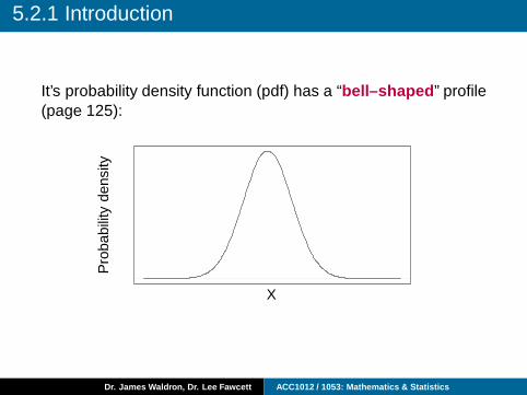
It’s probability density function (pdf) has a “bell–shaped ” profile(page 125):
Pro
babi
lity
dens
ity
X
Dr. James Waldron, Dr. Lee Fawcett ACC1012 / 1053: Mathematics & Statistics
5.2.1 Introduction
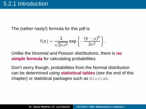
The (rather nasty!) formula for this pdf is
f (x) =1
√2πσ2
exp{
−(x − µ)2
2σ2
}
.
Unlike the binomial and Poisson distributions, there is nosimple formula for calculating probabilities.
Don’t worry though, probabilities from the Normal distributioncan be determined using statistical tables (see the end of thischapter) or statistical packages such as Minitab.
Dr. James Waldron, Dr. Lee Fawcett ACC1012 / 1053: Mathematics & Statistics
5.2.1 Introduction
There are four important characteristics of the Normaldistribution:
1 It is symmetrical about its mean, µ.
2 The mean, median and mode all coincide .
3 The area under the curve is equal to 1.
4 The curve extends in both directions to infinity (∞).
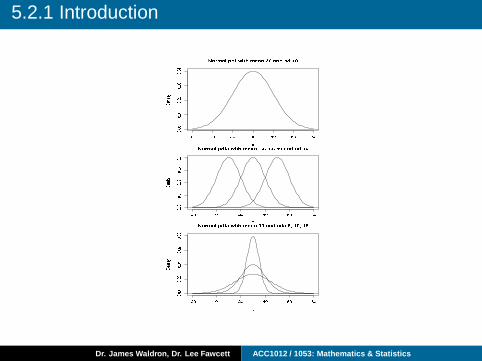
On the next slide are plots of the pdf for Normaldistributions with different values of µ and σ.
Dr. James Waldron, Dr. Lee Fawcett ACC1012 / 1053: Mathematics & Statistics
5.2.1 Introduction
Dr. James Waldron, Dr. Lee Fawcett ACC1012 / 1053: Mathematics & Statistics
5.2.2 Notation
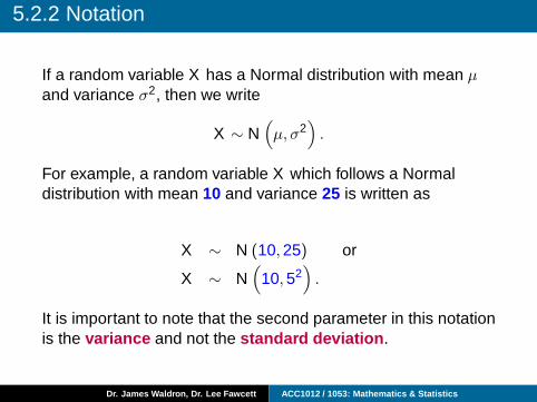
If a random variable X has a Normal distribution with mean µand variance σ2, then we write
X ∼ N(
µ, σ2)
.
For example, a random variable X which follows a Normaldistribution with mean 10 and variance 25 is written as
X ∼ N (10,25) or
X ∼ N(
10,52)
.
It is important to note that the second parameter in this notationis the variance and not the standard deviation .
Dr. James Waldron, Dr. Lee Fawcett ACC1012 / 1053: Mathematics & Statistics
5.2.3 The standard Normal distribution
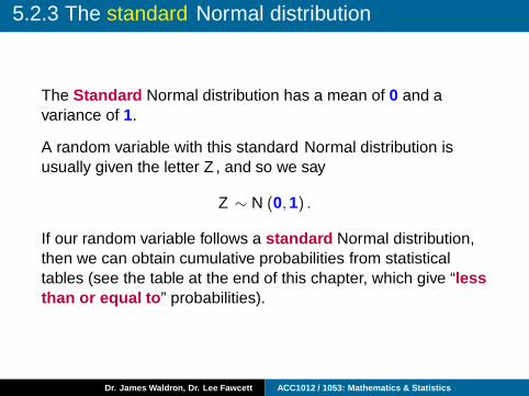
The Standard Normal distribution has a mean of 0 and avariance of 1.
A random variable with this standard Normal distribution isusually given the letter Z , and so we say
Z ∼ N (0,1) .
If our random variable follows a standard Normal distribution,then we can obtain cumulative probabilities from statisticaltables (see the table at the end of this chapter, which give “lessthan or equal to ” probabilities).
Dr. James Waldron, Dr. Lee Fawcett ACC1012 / 1053: Mathematics & Statistics
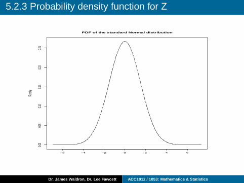
5.2.3 Probability density function for Z
−6 −4 −2 0 2 4 6
0.00
0.05
0.10
0.15
0.20
0.25
PDF of the standard Normal distributionDe
nsity
Dr. James Waldron, Dr. Lee Fawcett ACC1012 / 1053: Mathematics & Statistics
5.2.3 The standard Normal distribution
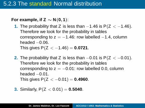
For example, if Z ∼ N(0,1):
1. The probability that Z is less than −1.46 is P(Z < −1.46).Therefore we look for the probability in tablescorresponding to z = −1.46: row labelled −1.4, columnheaded −0.06.This gives P(Z < −1.46) = 0.0721.
2. The probability that Z is less than −0.01 is P(Z < −0.01).Therefore we look for the probability in tablescorresponding to z = −0.01: row labelled 0.0, columnheaded −0.01.This gives P(Z < −0.01) = 0.4960.
3. Similarly, P(Z < 0.01) = 0.5040.
Dr. James Waldron, Dr. Lee Fawcett ACC1012 / 1053: Mathematics & Statistics
5.2.3 The standard Normal distribution
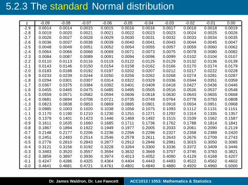
z -0.09 -0.08 -0.07 -0.06 -0.05 -0.04 -0.03 -0.02 -0.01 0.00-2.9 0.0014 0.0014 0.0015 0.0015 0.0016 0.0016 0.0017 0.0018 0.0018 0.0019-2.8 0.0019 0.0020 0.0021 0.0021 0.0022 0.0023 0.0023 0.0024 0.0025 0.0026-2.7 0.0026 0.0027 0.0028 0.0029 0.0030 0.0031 0.0032 0.0033 0.0034 0.0035-2.6 0.0036 0.0037 0.0038 0.0039 0.0040 0.0041 0.0043 0.0044 0.0045 0.0047-2.5 0.0048 0.0049 0.0051 0.0052 0.0054 0.0055 0.0057 0.0059 0.0060 0.0062-2.4 0.0064 0.0066 0.0068 0.0069 0.0071 0.0073 0.0075 0.0078 0.0080 0.0082-2.3 0.0084 0.0087 0.0089 0.0091 0.0094 0.0096 0.0099 0.0102 0.0104 0.0107-2.2 0.0110 0.0113 0.0116 0.0119 0.0122 0.0125 0.0129 0.0132 0.0136 0.0139-2.1 0.0143 0.0146 0.0150 0.0154 0.0158 0.0162 0.0166 0.0170 0.0174 0.0179-2.0 0.0183 0.0188 0.0192 0.0197 0.0202 0.0207 0.0212 0.0217 0.0222 0.0228-1.9 0.0233 0.0239 0.0244 0.0250 0.0256 0.0262 0.0268 0.0274 0.0281 0.0287-1.8 0.0294 0.0301 0.0307 0.0314 0.0322 0.0329 0.0336 0.0344 0.0351 0.0359-1.7 0.0367 0.0375 0.0384 0.0392 0.0401 0.0409 0.0418 0.0427 0.0436 0.0446-1.6 0.0455 0.0465 0.0475 0.0485 0.0495 0.0505 0.0516 0.0526 0.0537 0.0548-1.5 0.0559 0.0571 0.0582 0.0594 0.0606 0.0618 0.0630 0.0643 0.0655 0.0668-1.4 0.0681 0.0694 0.0708 0.0721 0.0735 0.0749 0.0764 0.0778 0.0793 0.0808-1.3 0.0823 0.0838 0.0853 0.0869 0.0885 0.0901 0.0918 0.0934 0.0951 0.0968-1.2 0.0985 0.1003 0.1020 0.1038 0.1056 0.1075 0.1093 0.1112 0.1131 0.1151-1.1 0.1170 0.1190 0.1210 0.1230 0.1251 0.1271 0.1292 0.1314 0.1335 0.1357-1.0 0.1379 0.1401 0.1423 0.1446 0.1469 0.1492 0.1515 0.1539 0.1562 0.1587-0.9 0.1611 0.1635 0.1660 0.1685 0.1711 0.1736 0.1762 0.1788 0.1814 0.1841-0.8 0.1867 0.1894 0.1922 0.1949 0.1977 0.2005 0.2033 0.2061 0.2090 0.2119-0.7 0.2148 0.2177 0.2206 0.2236 0.2266 0.2296 0.2327 0.2358 0.2389 0.2420-0.6 0.2451 0.2483 0.2514 0.2546 0.2578 0.2611 0.2643 0.2676 0.2709 0.2743-0.5 0.2776 0.2810 0.2843 0.2877 0.2912 0.2946 0.2981 0.3015 0.3050 0.3085-0.4 0.3121 0.3156 0.3192 0.3228 0.3264 0.3300 0.3336 0.3372 0.3409 0.3446-0.3 0.3483 0.3520 0.3557 0.3594 0.3632 0.3669 0.3707 0.3745 0.3783 0.3821-0.2 0.3859 0.3897 0.3936 0.3974 0.4013 0.4052 0.4090 0.4129 0.4168 0.4207-0.1 0.4247 0.4286 0.4325 0.4364 0.4404 0.4443 0.4483 0.4522 0.4562 0.4602-0.0 0.4641 0.4681 0.4721 0.4761 0.4801 0.4840 0.4880 0.4920 0.4960 0.5000
Dr. James Waldron, Dr. Lee Fawcett ACC1012 / 1053: Mathematics & Statistics
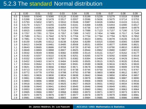
5.2.3 The standard Normal distribution
z 0.00 0.01 0.02 0.03 0.04 0.05 0.06 0.07 0.08 0.090.0 0.5000 0.5040 0.5080 0.5120 0.5160 0.5199 0.5239 0.5279 0.5319 0.53590.1 0.5398 0.5438 0.5478 0.5517 0.5557 0.5596 0.5636 0.5675 0.5714 0.57530.2 0.5793 0.5832 0.5871 0.5910 0.5948 0.5987 0.6026 0.6064 0.6103 0.61410.3 0.6179 0.6217 0.6255 0.6293 0.6331 0.6368 0.6406 0.6443 0.6480 0.65170.4 0.6554 0.6591 0.6628 0.6664 0.6700 0.6736 0.6772 0.6808 0.6844 0.68790.5 0.6915 0.6950 0.6985 0.7019 0.7054 0.7088 0.7123 0.7157 0.7190 0.72240.6 0.7257 0.7291 0.7324 0.7357 0.7389 0.7422 0.7454 0.7486 0.7517 0.75490.7 0.7580 0.7611 0.7642 0.7673 0.7704 0.7734 0.7764 0.7794 0.7823 0.78520.8 0.7881 0.7910 0.7939 0.7967 0.7995 0.8023 0.8051 0.8078 0.8106 0.81330.9 0.8159 0.8186 0.8212 0.8238 0.8264 0.8289 0.8315 0.8340 0.8365 0.83891.0 0.8413 0.8438 0.8461 0.8485 0.8508 0.8531 0.8554 0.8577 0.8599 0.86211.1 0.8643 0.8665 0.8686 0.8708 0.8729 0.8749 0.8770 0.8790 0.8810 0.88301.2 0.8849 0.8869 0.8888 0.8907 0.8925 0.8944 0.8962 0.8980 0.8997 0.90151.3 0.9032 0.9049 0.9066 0.9082 0.9099 0.9115 0.9131 0.9147 0.9162 0.91771.4 0.9192 0.9207 0.9222 0.9236 0.9251 0.9265 0.9279 0.9292 0.9306 0.93191.5 0.9332 0.9345 0.9357 0.9370 0.9382 0.9394 0.9406 0.9418 0.9429 0.94411.6 0.9452 0.9463 0.9474 0.9484 0.9495 0.9505 0.9515 0.9525 0.9535 0.95451.7 0.9554 0.9564 0.9573 0.9582 0.9591 0.9599 0.9608 0.9616 0.9625 0.96331.8 0.9641 0.9649 0.9656 0.9664 0.9671 0.9678 0.9686 0.9693 0.9699 0.97061.9 0.9713 0.9719 0.9726 0.9732 0.9738 0.9744 0.9750 0.9756 0.9761 0.97672.0 0.9772 0.9778 0.9783 0.9788 0.9793 0.9798 0.9803 0.9808 0.9812 0.98172.1 0.9821 0.9826 0.9830 0.9834 0.9838 0.9842 0.9846 0.9850 0.9854 0.98572.2 0.9861 0.9864 0.9868 0.9871 0.9875 0.9878 0.9881 0.9884 0.9887 0.98902.3 0.9893 0.9896 0.9898 0.9901 0.9904 0.9906 0.9909 0.9911 0.9913 0.99162.4 0.9918 0.9920 0.9922 0.9925 0.9927 0.9929 0.9931 0.9932 0.9934 0.99362.5 0.9938 0.9940 0.9941 0.9943 0.9945 0.9946 0.9948 0.9949 0.9951 0.99522.6 0.9953 0.9955 0.9956 0.9957 0.9959 0.9960 0.9961 0.9962 0.9963 0.99642.7 0.9965 0.9966 0.9967 0.9968 0.9969 0.9970 0.9971 0.9972 0.9973 0.99742.8 0.9974 0.9975 0.9976 0.9977 0.9977 0.9978 0.9979 0.9979 0.9980 0.99812.9 0.9981 0.9982 0.9982 0.9983 0.9984 0.9984 0.9985 0.9985 0.9986 0.9986
Dr. James Waldron, Dr. Lee Fawcett ACC1012 / 1053: Mathematics & Statistics
5.2.3 The standard Normal distribution
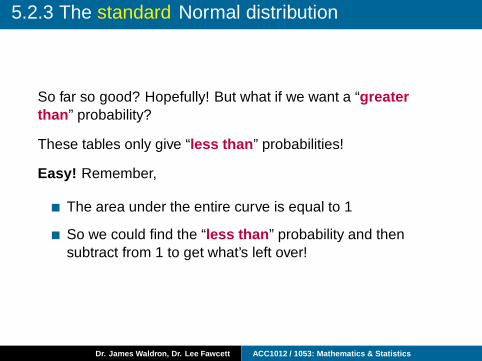
So far so good? Hopefully! But what if we want a “greaterthan ” probability?
These tables only give “less than ” probabilities!
Easy! Remember,
The area under the entire curve is equal to 1
So we could find the “less than ” probability and thensubtract from 1 to get what’s left over!
Dr. James Waldron, Dr. Lee Fawcett ACC1012 / 1053: Mathematics & Statistics
5.2.3 The standard Normal distribution
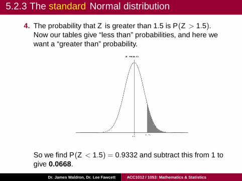
4. The probability that Z is greater than 1.5 is P(Z > 1.5).Now our tables give “less than” probabilities, and here wewant a “greater than” probability.
So we find P(Z < 1.5) = 0.9332 and subtract this from 1 togive 0.0668.
Dr. James Waldron, Dr. Lee Fawcett ACC1012 / 1053: Mathematics & Statistics
5.2.3 The standard Normal distribution
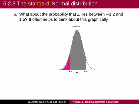
5. What about the probability that Z lies between −1.2 and1.5? It often helps to think about this graphically.
Doing so, gives:
P(−1.2 < Z < 1.5)= P(Z < 1.5)− P(Z < −1.2)
= 0.9332 − 0.1151
= 0.8181.Dr. James Waldron, Dr. Lee Fawcett ACC1012 / 1053: Mathematics & Statistics
5.2.3 The standard Normal distribution
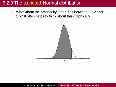
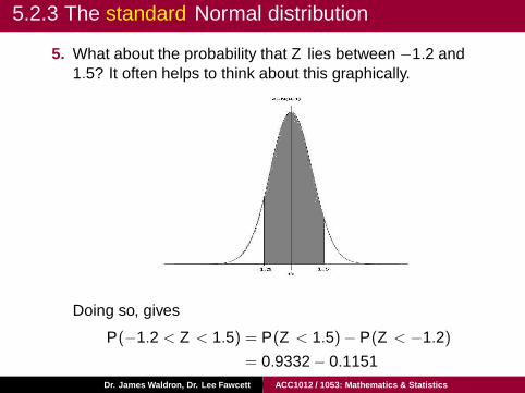
5. What about the probability that Z lies between −1.2 and1.5? It often helps to think about this graphically.
Doing so, gives
P(−1.2 < Z < 1.5) = P(Z < 1.5)− P(Z < −1.2)
= 0.9332 − 0.1151
= 0.8181.Dr. James Waldron, Dr. Lee Fawcett ACC1012 / 1053: Mathematics & Statistics
5.2.3 The standard Normal distribution
So how do we calculate probabilities for any Normaldistribution, not just the standard Normal distribution – forwhich we have tables?
Idea: “make” the Normal distribution that we have “look like” thestandard Normal distribution, and then we can just use thetables as before!
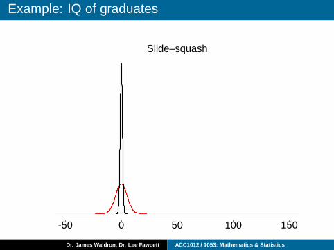
But how? Use the slide–squash technique!!
Dr. James Waldron, Dr. Lee Fawcett ACC1012 / 1053: Mathematics & Statistics
Example: IQ of graduates
The formula which changes any Normal random variable X intothe standard Normal random variable Z is given by
Z =X − µ
σ,
where
µ is the mean
σ is the standard deviation
This can be translated into probability statements:
P(X ≤ x) = P(
Z ≤x − µ
σ
)
Dr. James Waldron, Dr. Lee Fawcett ACC1012 / 1053: Mathematics & Statistics
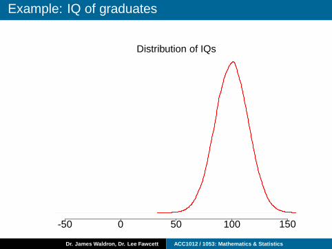
Example: IQ of graduates
Distribution of IQs
-50 0 50 100 150
Dr. James Waldron, Dr. Lee Fawcett ACC1012 / 1053: Mathematics & Statistics
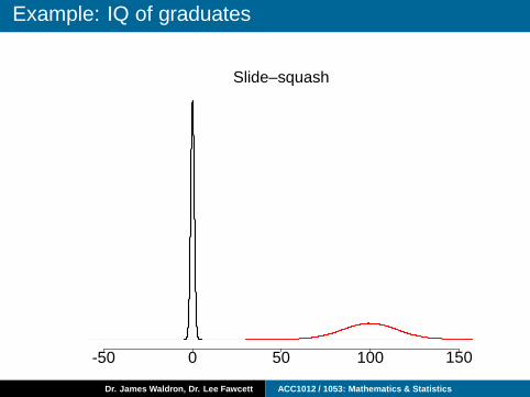
Example: IQ of graduates
Slide–squash
-50 0 50 100 150
Dr. James Waldron, Dr. Lee Fawcett ACC1012 / 1053: Mathematics & Statistics

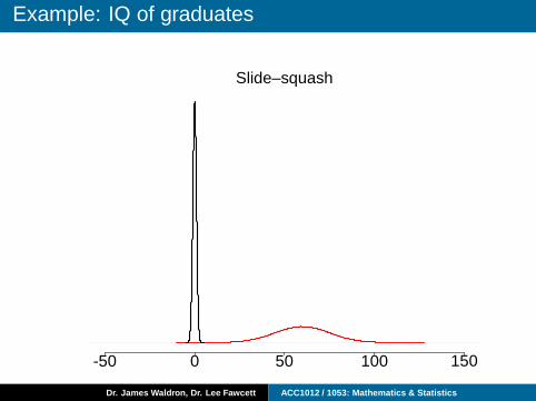
Example: IQ of graduates
Slide–squash
-50 0 50 100 150
Dr. James Waldron, Dr. Lee Fawcett ACC1012 / 1053: Mathematics & Statistics
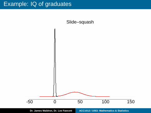
Example: IQ of graduates
Slide–squash
-50 0 50 100 150
Dr. James Waldron, Dr. Lee Fawcett ACC1012 / 1053: Mathematics & Statistics
Example: IQ of graduates
Slide–squash
-50 0 50 100 150
Dr. James Waldron, Dr. Lee Fawcett ACC1012 / 1053: Mathematics & Statistics

Example: IQ of graduates
Slide–squash
-50 0 50 100 150
Dr. James Waldron, Dr. Lee Fawcett ACC1012 / 1053: Mathematics & Statistics

Example: IQ of graduates
Slide–squash
-50 0 50 100 150
Dr. James Waldron, Dr. Lee Fawcett ACC1012 / 1053: Mathematics & Statistics
Example: IQ of graduates
Slide–squash
-50 0 50 100 150
Dr. James Waldron, Dr. Lee Fawcett ACC1012 / 1053: Mathematics & Statistics

Example: IQ of graduates
Slide–squash
-50 0 50 100 150
Dr. James Waldron, Dr. Lee Fawcett ACC1012 / 1053: Mathematics & Statistics

Example: IQ of graduates
Slide–squash
-50 0 50 100 150
Dr. James Waldron, Dr. Lee Fawcett ACC1012 / 1053: Mathematics & Statistics

Example: IQ of graduates
Slide–squash
-50 0 50 100 150
Dr. James Waldron, Dr. Lee Fawcett ACC1012 / 1053: Mathematics & Statistics

Example: IQ of graduates
Slide–squash
-50 0 50 100 150
Dr. James Waldron, Dr. Lee Fawcett ACC1012 / 1053: Mathematics & Statistics
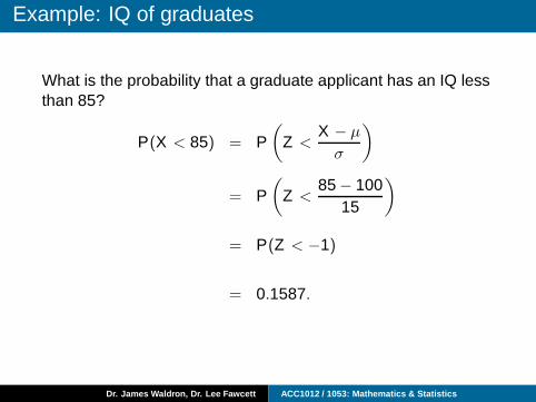
Example: IQ of graduates
What is the probability that a graduate applicant has an IQ lessthan 85?
P(X < 85) = P(
Z <X − µ
σ
)
= P(
Z <85 − 100
15
)
= P(Z < −1)
= 0.1587.
Dr. James Waldron, Dr. Lee Fawcett ACC1012 / 1053: Mathematics & Statistics
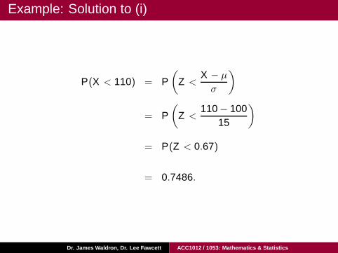
Example: Solution to (i)
P(X < 110) = P(
Z <X − µ
σ
)
= P(
Z <110 − 100
15
)
= P(Z < 0.67)
= 0.7486.
Dr. James Waldron, Dr. Lee Fawcett ACC1012 / 1053: Mathematics & Statistics
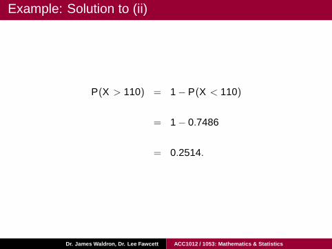
Example: Solution to (ii)
P(X > 110) = 1 − P(X < 110)
= 1 − 0.7486
= 0.2514.
Dr. James Waldron, Dr. Lee Fawcett ACC1012 / 1053: Mathematics & Statistics
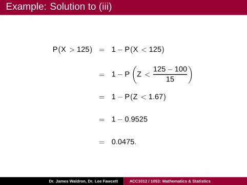
Example: Solution to (iii)
P(X > 125) = 1 − P(X < 125)
= 1 − P(
Z <125 − 100
15
)
= 1 − P(Z < 1.67)
= 1 − 0.9525
= 0.0475.
Dr. James Waldron, Dr. Lee Fawcett ACC1012 / 1053: Mathematics & Statistics
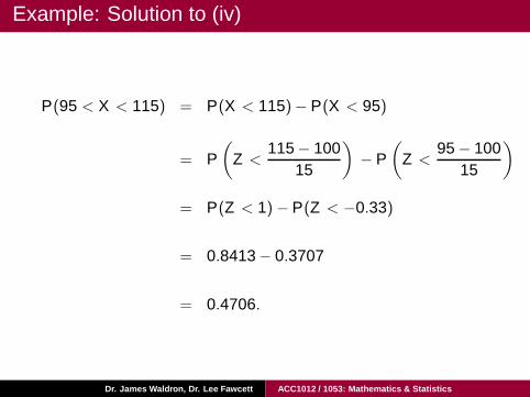
Example: Solution to (iv)
P(95 < X < 115) = P(X < 115)− P(X < 95)
= P(
Z <115 − 100
15
)
− P(
Z <95 − 100
15
)
= P(Z < 1)− P(Z < −0.33)
= 0.8413 − 0.3707
= 0.4706.
Dr. James Waldron, Dr. Lee Fawcett ACC1012 / 1053: Mathematics & Statistics
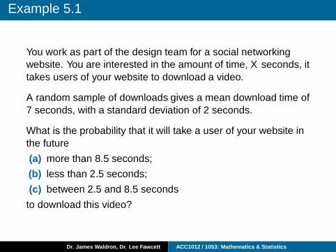
Example 5.1
You work as part of the design team for a social networkingwebsite. You are interested in the amount of time, X seconds, ittakes users of your website to download a video.
A random sample of downloads gives a mean download time of7 seconds, with a standard deviation of 2 seconds.
What is the probability that it will take a user of your website inthe future
(a) more than 8.5 seconds;
(b) less than 2.5 seconds;
(c) between 2.5 and 8.5 seconds
to download this video?
Dr. James Waldron, Dr. Lee Fawcett ACC1012 / 1053: Mathematics & Statistics
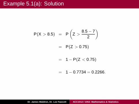
Example 5.1(a): Solution
P(X > 8.5) = P(
Z >8.5 − 7
2
)
= P(Z > 0.75)
= 1 − P(Z < 0.75)
= 1 − 0.7734 = 0.2266.
Dr. James Waldron, Dr. Lee Fawcett ACC1012 / 1053: Mathematics & Statistics
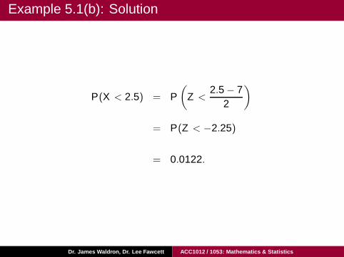
Example 5.1(b): Solution
P(X < 2.5) = P(
Z <2.5 − 7
2
)
= P(Z < −2.25)
= 0.0122.
Dr. James Waldron, Dr. Lee Fawcett ACC1012 / 1053: Mathematics & Statistics
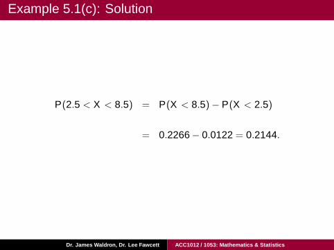
Example 5.1(c): Solution
P(2.5 < X < 8.5) = P(X < 8.5)− P(X < 2.5)
= 0.2266 − 0.0122 = 0.2144.
Dr. James Waldron, Dr. Lee Fawcett ACC1012 / 1053: Mathematics & Statistics
5.3 More Continuous Probability Models
Over the past few weeks we have discussed some “standard”probability distributions which can be used to model data.
We have looked at two such distributions for discrete data –the binomial distribution and the Poisson distribution – and lastweek the Normal distribution was introduced as a probabilitymodel for continuous data.
Dr. James Waldron, Dr. Lee Fawcett ACC1012 / 1053: Mathematics & Statistics
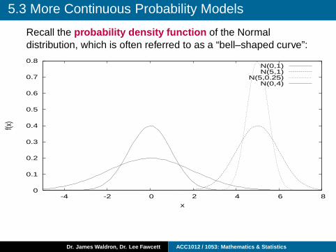
5.3 More Continuous Probability Models
Recall the probability density function of the Normaldistribution, which is often referred to as a “bell–shaped curve”:
0
0.1
0.2
0.3
0.4
0.5
0.6
0.7
0.8
-4 -2 0 2 4 6 8
f(x)
x
N(0,1)N(5,1)
N(5,0.25)N(0,4)
Dr. James Waldron, Dr. Lee Fawcett ACC1012 / 1053: Mathematics & Statistics
5.3 More Continuous Probability Models
We saw in the lecture last week that many naturally occurringcontinuous measurements (such as height, weight, time, rainfalletc.) often resemble this bell–shaped curve when plotted usinga histogram, for example.
But what if we cannot assume “Normality” for our data?
We now consider two other probability models which can beused to model continuous data when the Normal distributionisn’t appropriate.
Dr. James Waldron, Dr. Lee Fawcett ACC1012 / 1053: Mathematics & Statistics
5.3 Example of “non–Normality”
You manage a group of Environmental Health Officers andneed to decide at what time they should inspect a localhotel
You decide that any time during the working day (9.00 to18.00) is okay
You want to decide the time “randomly”
Here, “randomly ” is a short–hand for
“a random time, where all times in the working dayare equally likely to be chosen”
Dr. James Waldron, Dr. Lee Fawcett ACC1012 / 1053: Mathematics & Statistics
5.3.1 The Uniform distribution
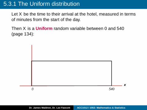
Let X be the time to their arrival at the hotel, measured in termsof minutes from the start of the day.
Then X is a Uniform random variable between 0 and 540(page 134):
Dr. James Waldron, Dr. Lee Fawcett ACC1012 / 1053: Mathematics & Statistics
5.3.1 The Uniform distribution
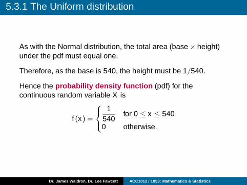
As with the Normal distribution, the total area (base × height)under the pdf must equal one.
Therefore, as the base is 540, the height must be 1/540.
Hence the probability density function (pdf) for thecontinuous random variable X is
f (x) =
1540
for 0 ≤ x ≤ 540
0 otherwise.
Dr. James Waldron, Dr. Lee Fawcett ACC1012 / 1053: Mathematics & Statistics
5.3.1 The Uniform distribution
In general, we say that a random variable X which is equallylikely to take any value between a and b has a uniformdistribution on the interval a to b, i.e.
X ∼ U(a,b).
Dr. James Waldron, Dr. Lee Fawcett ACC1012 / 1053: Mathematics & Statistics
5.3.1 The Uniform distribution
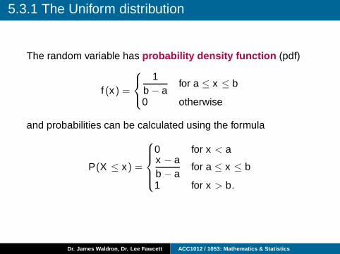
The random variable has probability density function (pdf)
f (x) =
1b − a
for a ≤ x ≤ b
0 otherwise
and probabilities can be calculated using the formula
P(X ≤ x) =
0 for x < ax − ab − a
for a ≤ x ≤ b
1 for x > b.
Dr. James Waldron, Dr. Lee Fawcett ACC1012 / 1053: Mathematics & Statistics
5.3.1 The Uniform distribution
Therefore, for example, the probability that the inspectorsvisit the hotel in the morning (within 180 minutes after 9am)is
P(X ≤ 180) =180 − 0540 − 0
=13.
Dr. James Waldron, Dr. Lee Fawcett ACC1012 / 1053: Mathematics & Statistics
5.3.1 The Uniform distribution
The probability of a visit during the lunch hour (12.30 to13.30) is
P(210 ≤ X ≤ 270) = P(X ≤ 270)− P(X < 210)
=270 − 0540 − 0
−210 − 0540 − 0
=270 − 210
540
=60540
=19.
Dr. James Waldron, Dr. Lee Fawcett ACC1012 / 1053: Mathematics & Statistics
5.3.1 Uniform distribution: Mean and Variance
Recall that:
If X ∼ bin(n,p), then
– E(X) = n × p and
– Var(X) = n × p × (1 − p)
If X ∼ Po(λ), then
– E(X) = λ and
– Var(X) = λ
Dr. James Waldron, Dr. Lee Fawcett ACC1012 / 1053: Mathematics & Statistics
5.3.1 Uniform distribution: Mean and Variance
We have equivalent formulae for X ∼ U(a,b):
E(X ) =a + b
2
Var(X ) =(b − a)2
12.
Dr. James Waldron, Dr. Lee Fawcett ACC1012 / 1053: Mathematics & Statistics
5.3.1 Uniform distribution: Mean and Variance
In the above example, we have
E(X ) =a + b
2=
0 + 5402
= 270,
so that the mean arrival of the inspectors is 9am + 270 minutes= 13.30.
Also
Var(X ) =(540 − 0)2
12= 24300,
and therefore SD(X ) =√
Var(X ) =√
24300 = 155.9 minutes.
Dr. James Waldron, Dr. Lee Fawcett ACC1012 / 1053: Mathematics & Statistics
5.3.2 The Exponential distribution
The exponential distribution is another common distributionthat is used to describe continuous random variables.
It is often used to model lifetimes of products and timesbetween “random” events, for example:
Lifetime of light bulbs
Arrival of customers in a queueing system
Arrival of orders
The distribution has one parameter, λ. If our random variable Xfollows an exponential distribution , then we say
X ∼ exp(λ).
Dr. James Waldron, Dr. Lee Fawcett ACC1012 / 1053: Mathematics & Statistics
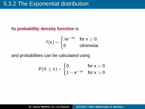
5.3.2 The Exponential distribution
Its probability density function is
f (x) =
{
λe−λx for x ≥ 0,
0 otherwise
and probabilities can be calculated using
P(X ≤ x) =
{
0 for x < 0
1 − e−λx for x > 0.
Dr. James Waldron, Dr. Lee Fawcett ACC1012 / 1053: Mathematics & Statistics
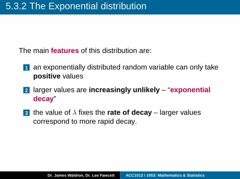
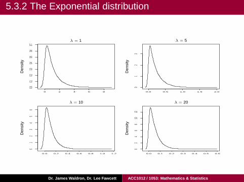
5.3.2 The Exponential distribution
The main features of this distribution are:
1 an exponentially distributed random variable can only takepositive values
2 larger values are increasingly unlikely – “exponentialdecay ”
3 the value of λ fixes the rate of decay – larger valuescorrespond to more rapid decay.
Dr. James Waldron, Dr. Lee Fawcett ACC1012 / 1053: Mathematics & Statistics
5.3.2 The Exponential distribution
0 2 4 6 8
0.00.1
0.20.3
0.40.5
0.60.7
0.0 0.5 1.0 1.5 2.0
01
23
0.0 0.2 0.4 0.6 0.8 1.0 1.2
01
23
45
6
0.0 0.1 0.2 0.3 0.4 0.5 0.6
02
46
810
12
Den
sity
Den
sity
Den
sity
Den
sity
λ = 1 λ = 5
λ = 10 λ = 20
Dr. James Waldron, Dr. Lee Fawcett ACC1012 / 1053: Mathematics & Statistics
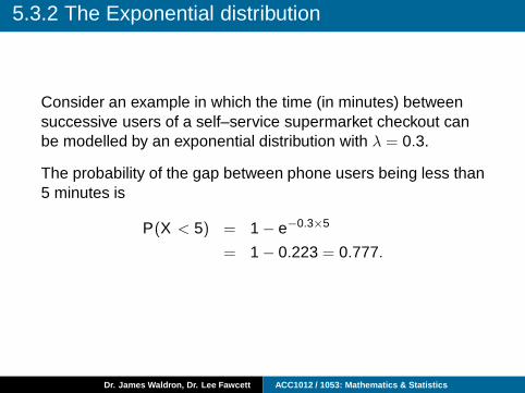
5.3.2 The Exponential distribution
Consider an example in which the time (in minutes) betweensuccessive users of a self–service supermarket checkout canbe modelled by an exponential distribution with λ = 0.3.
The probability of the gap between phone users being less than5 minutes is
P(X < 5) = 1 − e−0.3×5
= 1 − 0.223 = 0.777.
Dr. James Waldron, Dr. Lee Fawcett ACC1012 / 1053: Mathematics & Statistics
5.3.2 The Exponential distribution
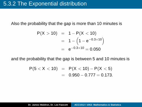
Also the probability that the gap is more than 10 minutes is
P(X > 10) = 1 − P(X < 10)
= 1 −(
1 − e−0.3×10)
= e−0.3×10 = 0.050
and the probability that the gap is between 5 and 10 minutes is
P(5 < X < 10) = P(X < 10)− P(X < 5)
= 0.950 − 0.777 = 0.173.
Dr. James Waldron, Dr. Lee Fawcett ACC1012 / 1053: Mathematics & Statistics
5.3.2 The Exponential distribution
One of the main uses of the exponential distribution is as amodel for the times between events occurring randomly intime .
We have previously considered events which occur at randompoints in time in connection with the Poisson distribution .
The Poisson distribution describes probabilities for the numberof events taking place in a given time period.
The exponential distribution describes probabilities for the timesbetween events. Both of these concern events occurringrandomly in time (at a constant average rate, say λ). This isknown as a Poisson process .
Dr. James Waldron, Dr. Lee Fawcett ACC1012 / 1053: Mathematics & Statistics
5.3.2 The Exponential distribution
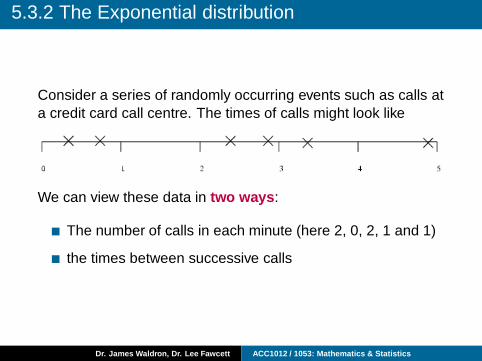
Consider a series of randomly occurring events such as calls ata credit card call centre. The times of calls might look like
We can view these data in two ways :
The number of calls in each minute (here 2, 0, 2, 1 and 1)
the times between successive calls
Dr. James Waldron, Dr. Lee Fawcett ACC1012 / 1053: Mathematics & Statistics
5.3.2 The Exponential distribution
For the Poisson process ,
the number of calls has a Poisson distribution withparameter λ, and
the time between successive calls has an exponentialdistribution with parameter λ.
Dr. James Waldron, Dr. Lee Fawcett ACC1012 / 1053: Mathematics & Statistics
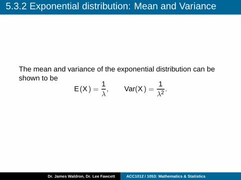
5.3.2 Exponential distribution: Mean and Variance
The mean and variance of the exponential distribution can beshown to be
E(X ) =1λ, Var(X ) =
1λ2 .
Dr. James Waldron, Dr. Lee Fawcett ACC1012 / 1053: Mathematics & Statistics
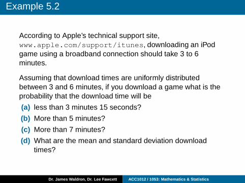
Example 5.2
According to Apple’s technical support site,www.apple.com/support/itunes, downloading an iPodgame using a broadband connection should take 3 to 6minutes.
Assuming that download times are uniformly distributedbetween 3 and 6 minutes, if you download a game what is theprobability that the download time will be
(a) less than 3 minutes 15 seconds?
(b) More than 5 minutes?
(c) More than 7 minutes?
(d) What are the mean and standard deviation downloadtimes?
Dr. James Waldron, Dr. Lee Fawcett ACC1012 / 1053: Mathematics & Statistics
Example 5.2(a): Solution
Let X : Time taken to download a game (minutes). ThenX ∼ U(3,6).
So
P(X < 3.25) =3.25 − 3
6 − 3=
112
= 0.0833.
Dr. James Waldron, Dr. Lee Fawcett ACC1012 / 1053: Mathematics & Statistics
Example 5.2(b),(c): Solution
Similarly,
P(X > 5) = 1 − P(X < 5)
= 1 −5 − 36 − 3
=13= 0.3333.
Also, P(X > 7) = 0... why?
Dr. James Waldron, Dr. Lee Fawcett ACC1012 / 1053: Mathematics & Statistics
Example 5.2(d): Solution
If X ∼ U(a,b),
E [X ] =a + b
2and Var(X ) =
(b − a)2
12.
So we have
E [X ] =3 + 6
2= 4.5 minutes
and
SD(X ) =
√
(6 − 3)2
12= 0.866 minutes
Dr. James Waldron, Dr. Lee Fawcett ACC1012 / 1053: Mathematics & Statistics
Example 5.3
Customers arrive at the drive–through window of a fast foodrestaurant at a rate of 2 per minute during the lunch hour.
(a) What is the probability that the next customer will arrivewithin 1 minute?
(b) What is the probability that the next customer will arrivewithin 20 seconds?
(c) What is the mean time between arrivals at thedrive–through window? What about the standarddeviation?
Dr. James Waldron, Dr. Lee Fawcett ACC1012 / 1053: Mathematics & Statistics
Example 5.3(a),(b): Solution
Let X : Time between arrivals at the drive–through window(minutes); X ∼ exp(2). Then
P(X < 1) = 1 − e−2×1
= 0.865.
Similarly,
P(
X <13
)
= 1 − e−2× 13
= 0.487
Dr. James Waldron, Dr. Lee Fawcett ACC1012 / 1053: Mathematics & Statistics
Example 5.3(c): Solution
If X ∼ exp(λ), then
E [X ] =1λ
and Var(X ) =1λ2 .
Thus, in our example,
E [X ] =12= 0.5 minutes = 30 seconds,
and
SD(X ) =
√
122 =
√
14= 30 seconds.
Dr. James Waldron, Dr. Lee Fawcett ACC1012 / 1053: Mathematics & Statistics