Abundance analysis of targets for the COROT/MONS

A&A 425, 683–695 (2004)DOI: 10.1051/0004-6361:20040464c© ESO 2004

Astronomy&

Astrophysics

Abundance analysis of targets for the COROT/MONSasteroseismology missions

II. Abundance analysis of the COROT main targets�

H. Bruntt1, I. F. Bikmaev2, C. Catala3, E. Solano4, M. Gillon5, P. Magain5, C. Van’t Veer-Menneret6,C. Stütz7, W. W. Weiss7, D. Ballereau6, J. C. Bouret8, S. Charpinet9, T. Hua8,

D. Katz6, F. Lignières9, and T. Lueftinger7

1 Department of Physics and Astronomy, Aarhus University, Bygn. 520, 8000 Aarhus C, Denmarke-mail: [email protected]

2 Department of Astronomy, Kazan State University, Kremlevskaya 18, 420008 Kazan, Russia3 Observatoire de Paris, LESIA, France4 Laboratorio de Astrofísica Espacial y Física Fundamental, PO Box 50727, 28080 Madrid, Spain5 Institut d’Astrophysique et de Géophysique, Université de Liège, Allée du 6 Août, 17, 4000 Liège, Belgium6 Observatoire de Paris, GEPI, France7 Institut für Astronomie, Universität Wien, Türkenschanzstrasse 17, 1180 Wien, Austria8 Laboratoire d’Astrophysique de Marseille, France9 Laboratoire d’Astrophysique de l’OMP, CNRS UMR 5572, Observatoire Midi-Pyrénées, 14, avenue Edouard Belin,

31400 Toulouse, France

Received 17 March 2004 / Accepted 11 June 2004

Abstract. One of the goals of the ground-based support program for the and / satellite missions is to charac-terize suitable target stars for the part of the missions dedicated to asteroseismology. We present the detailed abundance analysisof nine of the potential main targets using the semi-automatic software . For two additional targets we couldnot perform the analysis due to the high rotational velocity of these stars. For five stars with low rotational velocity we havealso performed abundance analysis by a classical equivalent width method in order to test the reliability of the software.The agreement between the different methods is good. We find that it is necessary to measure abundances extracted from eachline relative to the abundances found from a spectrum of the Sun in order to remove systematic errors. We have constrainedthe global atmospheric parameters Teff , log g, and [Fe/H] to within 70−100 K, 0.1−0.2 dex, and 0.1 dex for five stars which areslow rotators (v sin i < 15 km s−1). For most of the stars we find good agreement with the parameters found from line depthratios, Hα lines, Strömgren indices, previous spectroscopic studies, and also log g determined from the parallaxes.For the fast rotators (v sin i > 60 km s−1) it is not possible to constrain the atmospheric parameters.

Key words. stars: abundances – stars: fundamental parameters

1. Introduction

(COnvection, ROtation, and planetary Transits) is a smallspace mission, dedicated to asteroseismology and the searchfor exo-planets (Baglin et al. 2001). Among the targets of theasteroseismology part of the mission, a few bright stars will bemonitored continuously over a period of 150 days. These brighttargets will be chosen from a list of a dozen F & G-type stars,located in the continuous viewing zone of the instrument. Thefinal choice of targets needs to be made early in the project, as itwill impact on some technical aspects of the mission. A preciseand reliable knowledge of the candidate targets is required, inorder to optimize this final choice.

� Based on observations obtained with the 193 cm telescope atObservatoire de Haute Provence, France.

Among the information which needs to be gathered on thecandidate targets, fundamental parameters like effective tem-perature, surface gravity, and metallicity will play a major rolein the selection of targets for . Projected rotation veloci-ties, as well as detailed abundances of the main chemical ele-ments will also be taken into account in the selection process.Thus, the aim of this study is to obtain improved values for thefundamental parameters and abundances of individual elementsfor the main targets.

This information on the targets will subsequently be usedfor the selected stars, in conjunction with asteroseismologicaldata obtained by , to provide additional constraints for themodelling of the interior and the atmospheres of these stars.

In Sect. 2 we summarize the spectroscopic observationsand data reduction, in Sect. 3 we discuss the determination

Article published by EDP Sciences and available at http://www.aanda.org or http://dx.doi.org/10.1051/0004-6361:20040464

http://www.edpsciences.org/

http://www.aanda.org

http://dx.doi.org/10.1051/0004-6361:20040464

684 H. Bruntt et al.: Abundance analysis of targets for the COROT/MONS asteroseismology missions. II.

Table 1. Log of the observations for the spectra of the proposed targets we have analysed. The signal-to-noise ratio in the last columnis calculated around 6500 Å in bins of 3 km s−1.

HD Date UT start texp S/N43318 19-Jan.-98 22:38 900 12043587 14-Jan.-98 22:32 1800 25045067 15-Jan.-98 22:20 1200 26049434 17-Jan.-98 22:33 600 16049933 21-Jan.-98 22:17 1200 21055057 15-Jan.-98 23:10 900 27057006 10-Dec.-00 00:41 1800 250

171834 05-Sep.-98 19:00 1800 300184663 18-Jun.-00 01:30 1000 170

46304 17-Jan.-98 22:05 600 170174866 04-Jul.-01 00:39 1500 190

of the fundamental parameters from spectroscopy, photometryand parallaxes and we summarize previous spectro-scopic studies of the target stars. In Sect. 4 we describe thethree different methods we have used for abundance analysis.In Sect. 5 we discuss how we constrain the fundamental atmo-spheric parameters using abundance results for a grid of mod-els. In Sect. 6 we discuss the abundances we have determined.Lastly, we give our conclusions in Sect. 7.

2. Spectroscopic observations

We have obtained spectra of each one of the 11 candidate maintargets of , using the spectrograph attached to the1.93 m telescope at Observatoire de Haute-Provence (OHP). is a fiber-fed cross-dispersed Echelle spectrograph, pro-viding a complete spectral coverage of the 3800–6800 Å re-gion, at a resolution of R = 45 000 (Baranne et al. 1996).Table 1 gives the log of the observations for the spectra usedin this analysis.

2.1. Data reduction

We used the on-line - reduction package available atOHP (Baranne et al. 1996). This software performs bias andbackground light subtraction, spectral order localization, andfinally extracts spectral orders using the optimal extraction pro-cedure (Horne 1986). The high spatial frequency instrumentalresponse is corrected by dividing the stellar spectra by the spec-trum of a flat-field lamp. Wavelength calibration is provided byspectra of a Th/Ar lamp, using a two-dimensional Chebychevpolynomial fitting to the centroid locations of the Th/Ar lines.

Special care was taken to correct for the grating blaze func-tion, as differences in the spectrograph illumination betweenstellar and flat-field light beams usually result in an imper-fect correction. Instead of using a flat-field spectrum, we havetherefore used a high signal-to-noise spectrum of an O-typestar, 10 Lac, to determine the blaze function. The orders ofthe 10 Lac spectrum were examined one by one, and the line-free regions of each order were identified. The blaze function ateach spectrograph order was then represented by cubic splinesfitted to these line-free regions, and the stellar spectra were

Table 2. Strömgren photometric indices of the main targetstaken from Hauck & Mermilliod (1998). HD 46304 and HD 174866are shown separately: abundance analysis has not been made for thesetwo stars due to their high v sin i.

HD V b − y m1 c1 Hβ43318 5.65 0.322 0.154 0.446 2.64443587 5.70 0.384 0.187 0.349 2.60145067 5.87 0.361 0.168 0.396 2.61149434 5.74 0.178 0.178 0.717 2.75549933 5.76 0.270 0.127 0.460 2.66255057 5.45 0.185 0.184 0.876 2.75757006 5.91 0.340 0.168 0.472 2.625

171384 5.45 0.254 0.145 0.560 2.682184663 6.37 0.275 0.149 0.476 2.66546304 5.60 0.158 0.175 0.816 2.767

174866 6.33 0.122 0.178 0.960 2.822

subsequently divided by this newly determined blaze function.This procedure results in an adequate blaze correction, produc-ing in particular a good match of adjacent orders in the overlap-ping regions. Note also that is a very stable instrument,so that only one spectrum of 10 Lac was used to define the blazefunction, although the observations reported here span severalyears.

Since the overall blaze function was removed by a star ofmuch earlier spectral class than the observed F and G-type starsthe continuum level was not entirely flat. Hence we made cubicspline fits to make the final continuum estimate. For the over-lapping part of the orders we made sure that the overlap wasbetter than 0.5%.

We are aware of the problem of fitting low-order splinesto correct the continuum. In this process we manually markthe points in the spectrum which we assume are at the contin-uum level. When using the software (Bruntt et al. 2002, cf.Sect. 4.2) we can inspect the fitted lines and in this way detectproblems with the continuum level. In these cases we reject theabundances found for these lines (cf. Sect. 4.5). Alternatively,one could select “continuum windows” from a synthetic spec-trum or a spectrum of the Sun and use this to correct the con-tinuum level. This has been attempted for one of our programstars in Sect. 4.4.

3. Fundamental atmospheric parameters

In this section we will discuss previous results for the funda-mental atmospheric parameters of the proposed targets.We will present the results from the calibration of Strömgrenphotometry, line depth ratios, Hα line wings, and parallaxes.

3.1. Strömgren photometry

The Strömgren indices of the target stars are taken from the cat-alogue of Hauck & Mermilliod (1998) and are listed in Table 2.We have used the software (Rogers 1995; see alsoKupka & Bruntt 2001) to find the appropriate calibration to ob-tain the basic parameters, i.e. Teff, log g, and [M/H]phot. These

H. Bruntt et al.: Abundance analysis of targets for the COROT/MONS asteroseismology missions. II. 685

Table 3. Overview of the parameters of the proposed main targets. The first column is the HD number and column 2 is Teff determinedfrom line depth ratios with formal errors in parenthesis (Kovtyukh et al. 2003). Column 3 gives the temperatures found from the Hα wings (theinternal error is 50 K). Columns 4–6 are the atmospheric parameters derived from Strömgren photometry when using the software(typical errors are 200 K, 0.3 dex, and 0.2 dex). Columns 7 and 8 are the masses found from evolution tracks (cf. Fig. 1) and log gπ values foundfrom the parallaxes; the numbers in parenthesis are the estimated standard errors. In Col. 9 we list v sin i where the typical error is5–10%.

Line depth Hα Strömgren Evolution tracks & Spectralratio wings indices parallax synthesis

HD Teff [K] Teff [K] Teff [K] log g [M/H]phot M/M� log gπ v sin i [km s−1]Sun 5770(5) − 5778a 4.44a +0.00a 1a 4.44a 2b

43318 6191(17) 6100 6400 4.19 −0.15 1.23(17) 3.96(14) 843587 5923(8) 5850 5931 4.31 −0.11 1.02(20) 4.29(15) 2.5b

45067 6067(6) 5900 6038 4.03 −0.22 1.08(17) 3.96(15) <7b

49434 − 6950 7304 4.14 −0.01 1.55(14) 4.25(11) 8449933 − 6400 6576 4.30 −0.45 1.17(18) 4.20(14) 1455057 − 6750 7274 3.61 +0.10 2.12(22) 3.66(12) 12057006 6181(7) 6000 6158 3.72 −0.13 1.28(17) 3.58(16) 9

171834 − 6550 6716 4.03 −0.22 1.40(17) 4.13(13) 63184663 − 6450 6597 4.25 −0.17 1.29(14) 4.19(15) 53

46304 − 7050 7379 3.93 −0.09 1.68(14) 4.18(11) 200174866 − 7200 7865 3.86 −0.18 1.77(14) 3.86(15) 165

a The fundamental parameters for the Sun are also given in the table, although we have notdetermined its parameters; the exception is our estimate of Teff from line depth ratios.b With the resolution of the spectrograph (R = 45 000) it is not possible to measurev sin i below 7 km s−1 directly.

parameters are given in Table 3. The accuracy of the parame-ters Teff, log g, and [M/H]phot are around 200–250 K, 0.3 dex,and 0.2 dex according to Rogers (1995).

A catalogue of Strömgren indices determined for all pri-mary and secondary targets for is available from the database1. We also used these data to get the fundamentalparameters. For most stars both Teff and log g agree within theuncertainties quoted above. But for HD 43587 and HD 45067we find a large discrepancy, i.e. log g higher by 0.2/0.3 dex anda higher Teff by 350/300 K for the two stars, respectively. Thisis a clear indication that it is worthwhile to use several methodsto try to determine the fundamental parameters.

3.2. Temperature calibration from line depth ratios

Kovtyukh et al. (2003) have used spectra of 181 main sequenceF-K type stars to calibrate the dependence of line depth ratioson Teff . They used observed spectra from ELODIE (the samespectrograph we used) and their sample of stars consisted ofstars for which Teff is well determined, e.g. using the infraredflux method.

We measured line depths by fitting a Gaussian profile toeach line, i.e. the depth of the Gaussian defines the line depth.We used Teff from the Strömgren photometry as our initialguess (assuming the error is σ(Teff) = 250 K) to select whichof the calibrations by Kovtyukh et al. (2003) that were valid.We note that for each pair of lines defining the ratio calibra-tion the species of elements are typically different (e.g. Si/Ti,Fe/S etc.), but we refer to Kovtyukh et al. (2003) for details.

1 http://sdc.laeff.esa.es/gaudi/

Typically 50–80 line depth ratios between lines could be used.We then calculated the mean Teff and rejected 3σ outliers andrecalculated Teff. The calibrations are only valid in the range4000–6150 K so only the four coolest target stars couldbe used with this method.

The results are given in Table 3 for these stars and the Sun.The Teff we determine from the spectrum of the Sun agreeswith the canonical value of Teff = 5777 K. The quoted errors of5–17 K on the temperatures are formal errors, and systematicerrors of the order 50–100 K must be added.

3.3. Temperatures from Hα lines

We have estimated Teff of the stars considered in this study us-ing their Hα line profiles, following a method proposed byCayrel et al. (1985) and Cayrel de Strobel et al. (1994). Themethod is based on the property of Hα that it is insensitive toany atmospheric parameter except Teff in in the range between5000–8500 K.

In order to overcome problems due to continuum place-ment, we compute the ratio of the observed Hα profile to thatof the Sun, observed with the same instrumental configuration(spectrum of the solar reflected light on the moon surface),then compare it to the corresponding ratio of theoretical pro-files computed from a grid of models. The best fit betweencomputed and observed profile ratios gives the effective tem-perature with an internal error bar of about ±50 K.

We have used the new grids of 9 models presented inHeiter et al. (2002), choosing the models with MLT convectiontreatment for Teff lower than 8750 K, with the low value for


the efficiency parameter of the convection, following Fuhrmannet al. (1993), Axer et al. (1994), and Heiter et al. (2002).

The Hα line profile is computed using 9 (Kurucz1998) which includes the Vidal et al. (1973) unified theory forthe Stark Broadening and also takes into account the self reso-nance mechanism in the computation of the Hα profile.

This method if found to be reliable for Teff between 5500and 8500 K. Below 5500 K, the Hα profile is not sensitiveenough to Teff, and does not constitute a good temperaturetracer. Above 8500 K, the Hα wings depend only slightlyon Teff , and start to become sensitive to gravity.

We find that the final Teff estimate is insensitive to thechoice of convection description. On the other hand Heiter et al.(2002) find that the (b− y) index and hence Teff found from theStrömgren indices is sensitive to the convection description.

The Teff measurements with this method are also reason-ably insensitive to rotation, for v sin i below 80–100 km s−1.

3.4. Comparison of temperature estimators

Except for HD 43318 there is very good agreement betweenTeff from the Strömgren calibration () and the linedepth ratios. However, Teff of HD 43318 is on the border of thevalid range of the latter calibration. The Teff from the Hα linesagrees with the other two methods but only for stars with lowv sin i. The stars in our sample with moderate v sin i also havethe highest Teff, and the discrepant results for the Hα lines maybe an indication that this method cannot be used for these stars.

3.5. Using HIPPARCOS parallaxes to determine log g

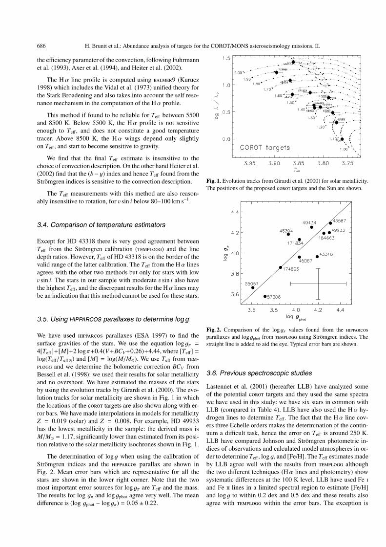
We have used parallaxes (ESA 1997) to find thesurface gravities of the stars. We use the equation log gπ =4[Teff]+[M]+2 logπ+0.4(V+BCV+0.26)+4.44, where [Teff] =log(Teff/Teff �) and [M] = log(M/M�). We use Teff from - and we determine the bolometric correction BCV fromBessell et al. (1998): we used their results for solar metallicityand no overshoot. We have estimated the masses of the starsby using the evolution tracks by Girardi et al. (2000). The evo-lution tracks for solar metallicity are shown in Fig. 1 in whichthe locations of the targets are also shown along with er-ror bars. We have made interpolations in models for metallicityZ = 0.019 (solar) and Z = 0.008. For example, HD 49933has the lowest metallicity in the sample: the derived mass isM/M� = 1.17, significantly lower than estimated from its posi-tion relative to the solar metallicity isochrones shown in Fig. 1.

The determination of log g when using the calibration ofStrömgren indices and the parallax are shown inFig. 2. Mean error bars which are representative for all thestars are shown in the lower right corner. Note that the twomost important error sources for log gπ are Teff and the mass.The results for log gπ and log gphot agree very well. The meandifference is (log gphot − log gπ) = 0.05 ± 0.22.

Fig. 1. Evolution tracks from Girardi et al. (2000) for solar metallicity.The positions of the proposed targets and the Sun are shown.

Fig. 2. Comparison of the log gπ values found from the parallaxes and log gphot from using Strömgren indices. Thestraight line is added to aid the eye. Typical error bars are shown.

3.6. Previous spectroscopic studies

Lastennet et al. (2001) (hereafter LLB) have analyzed someof the potential targets and they used the same spectrawe have used in this study: we have six stars in common withLLB (compared in Table 4). LLB have also used the Hα hy-drogen lines to determine Teff. The fact that the Hα line cov-ers three Echelle orders makes the determination of the contin-uum a difficult task, hence the error on Teff is around 250 K.LLB have compared Johnson and Strömgren photometric in-dices of observations and calculated model atmospheres in or-der to determine Teff, log g, and [Fe/H]. The Teff estimates madeby LLB agree well with the results from althoughthe two different techniques (Hα lines and photometry) showsystematic differences at the 100 K level. LLB have used Fe and Fe lines in a limited spectral region to estimate [Fe/H]and log g to within 0.2 dex and 0.5 dex and these results alsoagree with within the error bars. The exception is


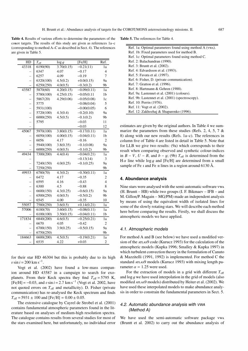
Table 4. Results of various efforts to determine the parameters of the targets. The results of this study are given as references 1a–c(corresponding to method A–C as described in Sect. 4). The referencesare given in Table 5.

HD Teff log g [Fe/H] Ref.43318 6190(90) 3.70(0.15) −0.21(11) 1a

– 6347 4.07 −0.17 4– 6257 4.09 −0.19 7– 6320(100) 4.5(0.2) +0.0(0.15) 9a– 6250(250) 4.0(0.5) −0.3(0.2) 9b

43587 5870(60) 4.20(0.15) −0.09(0.11) 1a– 5780(100) 4.25(0.15) −0.05(0.11 1b– 5867(20) 4.29(0.06) −0.05(0.08) 1c– 5775 −0.08(0.04) 5– 5931(100) −0.00(0.05) 6– 5720(100) 4.3(0.4) −0.2(0.10) 9a– 6000(250) 4.5(0.5) −0.1(0.2) 9b– 5795 −0.03 11– −0.03 12

45067 5970(100) 3.80(0.15) −0.17(0.11) 1a– 6050(100) 4.00(0.15) −0.04(0.11) 1b– 6056 4.17 −0.16 2– 5940(100) 3.8(0.35) −0.1(0.08) 9a– 6000(250) 4.0(0.5) −0.1(0.2) 9b

49434 7300(200) 4.4(0.4) −0.04(0.21) 1a– −0.13(14) 3– 7240(150) 4.0(0.25) −0.1(0.25) 9a– 7250(250) 9b

49933 6780(70) 4.3(0.2) −0.30(0.11) 1a– 6472 4.17 −0.35 2– 6595 4.16 −0.43 4– 6300 4.5 −0.88 8– 6600(150) 4.3(0.25) −0.6(0.15) 9a– 6500(250) 4.0(0.5) −0.5(0.2) 9b– 6545 4.00 −0.35 10

55057 7580(250) 3.6(0.5) +0.14(0.21) 1a57006 6180(70) 3.60(0.15) −0.08(0.11) 1a

– 6100(100) 3.50(0.15) −0.04(0.11) 1b171834 6840(200) 4.6(0.5) −0.25(0.21) 1a

– 6670 4.05 −0.42 2– 6700(150) 3.9(0.25) −0.5(0.15) 9a– 6750(250) 9b

184663 6600(200) 4.5(0.5) −0.19(0.21) 1a– 6535 4.22 +0.03 2

for their star HD 46304 but this is probably due to its highv sin i= 200 km s−1.

Vogt et al. (2002) have found a low-mass compan-ion around HD 43587 in a campaign to search for exo-planets. From their Keck spectra they find Teff = 5795 K,[Fe/H]=−0.03, and v sin i= 2.7 km s−1 (Vogt et al. 2002, havenot quoted errors on Teff and metallicity). D. Fisher (privatecommunication) has re-analysed the Keck spectrum and findsTeff = 5931 ± 100 and [Fe/H] = 0.00 ± 0.05.

The extensive catalogue by Cayrel de Strobel et al. (2001)contains fundamental atmospheric parameters found in the lit-erature based on analyses of medium-high resolution spectra.The catalogue contains results from several studies for most ofthe stars examined here, but unfortunately, no individual error

Table 5. The references for Table 4.

Ref. 1a: Optimal parameters found using method A ().Ref. 1b: Fixed parameters used for method B.Ref. 1c: Optimal parameters found using method C.Ref. 2: Balachandran (1990).Ref. 3: Bruntt et al. (2002).Ref. 4: Edvardsson et al. (1993).Ref. 5: Favata et al. (1997).Ref. 6: Fisher, D. (private communication).Ref. 7: Gratton et al. (1996).Ref. 8: Hartmann & Gehren (1988).Ref. 9a: Lastennet et al. (2001) (colours).Ref. 9b: Lastennet et al. (2001) (spectroscopy).Ref. 10: Perrin (1976).Ref. 11: Vogt et al. (2002).Ref. 12: Zakhozhaj & Shaparenko (1996).

estimates are given by the original authors. In Table 4 we sum-marize the parameters from these studies (Refs. 2, 4, 5, 7 &8) along with our new results (Refs. 1a–c). The references incolumn five of Table 4 are listed in detail in Table 5. Note thatfor LLB we give two results: (9a) which corresponds to theirresult when comparing observed and synthetic colour-indicesin B − V , U − B, and b − y; (9b) Teff is determined from theHα line while log g and [Fe/H] are determined from a smallsample of Fe and Fe lines in a region around 6130 Å.

4. Abundance analysis

Nine stars were analysed with the semi-automatic software (H. Bruntt – HB) while two groups (I. F. Bikmaev – IFB – andM. Gillon/P. Magain – MG/PM) made an independent analysisby means of using the equivalent width of isolated lines forsome of the slowly rotating stars. We will describe each methodhere before comparing the results. Firstly, we shall discuss theatmospheric models we have applied.

4.1. Atmospheric models

For method A and B (see below) we have used a modified ver-sion of the 9 code (Kurucz 1993) for the calculation of theatmospheric models (Kupka 1996; Smalley & Kupka 1997) inwhich turbulent convection theory in the formulation of Canuto& Mazzitelli (1991, 1992) is implemented. For method C thestandard 9 models (Kurucz 1993) with mixing length pa-rameter α = 1.25 were used.

For the extraction of models in a grid with different Teff

and log gwe have used interpolation in the grid of models (alsomodified 9 models) distributed by Heiter et al. (2002). Wehave used these interpolated models to make abundance analy-sis in order to constrain the fundamental parameters in Sect. 5.

4.2. Automatic abundance analysis with VWA

(Method A)

We have used the semi-automatic software package (Bruntt et al. 2002) to carry out the abundance analysis of


nine targets. For each star the software selects the leastblended lines from atomic line list data extracted from the data base (Kupka et al. 1999). The atomic data consistof the element name and ionization state, wavelength, exci-tation potential, oscillator strength, and damping parameters.For each selected line the synthetic spectrum is calculated andthe input abundance is changed iteratively until the equiva-lent width of the observed and synthetic line match. We used (version 2.5, see Valenti & Piskunov 1996) to calculatethe synthetic spectrum. This software was kindly provided byN. Piskunov (private communication).

4.2.1. Rotational velocities

In order to be able to compare the observed and synthetic spec-tra the latter is convolved by the instrumental profile (approxi-mated by a Gaussian) and a rotational broadening profile. Theprojected rotational velocities were determined by fittingthe synthetic spectrum of a few of the least blended lines tothe observed spectrum by convolving with different rotationprofiles. Note that we have used zero macroturbulence, andthus our quoted values for v sin i is a combination of the ef-fects of rotational broadening and macroturbulence. The accu-racy of v sin i by this method is about 5–10%. LLB used a morerefined method (see Donati et al. 1997) but our results agreewithin the estimated errors. The exception is for HD 43587 forwhich we have found 7 km s−1 while Vogt et al. (2002) findv sin i= 2.7 km s−1. Note that D. Fisher finds v sin i= 2.2 km s−1

from the same spectrum (private communication). These lowervalues agrees with LLB and consequently we have used a lowvalue of v sin i= 2.5 km s−1. The reason for the apparent dis-crepancy is simply the limit of the spectral resolution of the spectrograph i.e. v = c/R � 7 km s−1. Note that since relies on the measurement of equivalent widths small er-rors in v sin i will have a negligible effect on the derived abun-dances.

4.2.2. Measuring abundances relative to the Sun

During our analyses with we have found that when mea-suring abundances relative to the same lines observed in theSun there is a dramatic decrease in the error. Since the abun-dance of the Sun is well-known (e.g., Grevesse & Sauval 1998)we have decided to make a differential analysis. There are sev-eral sources of error that may affect the derived abundances butthe most important error is erroneous log g f values. Incorrectremoval of scattered light when reducing the spectra will causesystematic errors.

In Fig. 3 we show the iron abundance for several lines ver-sus both equivalent width and lower excitation potential forHD 57006. In the top panel we show the direct results whilein the bottom panel the abundances are measured relative tothe results for the Sun (line-by-line). For the zero point weused log NFe/Ntot = −4.54 from Grevesse & Sauval (1998).The open symbols are used for neutral ion lines (Fe ) and filledsymbols for ionized Fe lines (Fe ).

Fig. 3. Iron abundances from lines in the spectrum of HD 57006. Opensymbols are neutral iron lines and solid symbols are Fe lines. Thetop panel shows the raw abundances while in the bottom panel theabundances are relative to the abundances (line-by-line) found for theSun. The abundances are plotted versus equivalent width and excita-tion potential. The mean abundances and standard deviation are givenin each panel and the atmospheric model parameters are found in theboxes. The straight lines are linear fits to the neutral iron lines and thedashed curves indicate the 3σ interval for the fit.

Note the dramatic ∼40% decrease in the uncertainty for theneutral ion lines when measuring relative to the Sun (bottompanel in Fig. 3). Also, the discrepancy in abundance found fromFe and Fe lines is removed. For the applied atmosphericmodel of HD 57006 there is no correlation with either equiv-alent width nor excitation potential. Also, both Fe and Fe give the same result which indicates that the applied model iscorrect.

For the results presented in this work we have measuredabundances relative to the abundance found for the same linesin the spectrum of the Sun. However, we have not done thisfor the star HD 49933 and the stars with higher v sin i sincewe see no significant improvement for these stars. The rea-son is that these stars are much hotter than the reference star(∆Teff > 1000 K). This means that the Sun and the hotterstars have relatively few lines in common which are suitablefor abundance analysis. However, it is likely that this is an in-dication of inadequacies of the model atmospheres.

4.2.3. Adjusting the microturbulence

For each model we adjust the microturbulence ξt until we seeno correlation between the abundances and equivalent widthsfound for the Fe , Cr , and Ni lines. To minimize the effectof saturated lines we only use lines with equivalent width below100 mÅ and for Fe we only use lines with excitation potentialin the range 2–5 eV to minimize the effect of erroneous Teff ofthe model atmosphere. For some stars only Fe could be useddue to a lack of non-blended Cr and Ni lines. For the slowlyrotating stars (v sin i < 25 km s−1) the error on ξt is about0.1−0.2 km s−1, for the stars rotating moderately fast (50 <v sin i< 85 km s−1) the error is 0.5 km s−1, and 0.7 km s−1 for


HD 55057 which has v sin i = 120 km s−1. The contribution tothe error on the abundances from the uncertainty of the micro-turbulence is about 0.03 dex for Fe for the slow rotators whilefor stars with the highest v sin i (HD 49434 and HD 55057) theerrors in the abundances are of the order 0.07–0.10 dex.

For each star we made the abundance analysis for a grid ofmodels in order to be able to constrain Teff and log g which willbe discussed in Sect. 5.

4.3. “Classical” abundance analysis (Method B)

“Classical” abundance analysis was applied (IFB) to three ofthe slowly rotating targets – HD 43587, HD 45067, andHD 57006 – and to the solar spectrum (observed reflectionfrom the Moon).

Model atmospheres were calculated as described inSect. 4.1 with the adopted parameters of Teff , log g, and so-lar composition. Effective temperatures were determined by us-ing Johnson and Strömgren color-indices extracted from data base and the log g parameters were determined by using parallaxes as outlined in Sect. 3.5. The values wehave used are given in Table 4 marked with Ref. 1b. These pa-rameters were not changed during our analysis with method B.

Equivalent widths of all identified unblended and somepartially blended spectral lines were measured by using software based on PC (Galazutdinov 1992). Abundance cal-culations were performed in the LTE approximation by using9 (Kurucz 1993; with modifications by V. Tsymbal andL. Mashonkina for PC, private communication). Atomic pa-rameters of the spectral lines were extracted from the database with corrections of oscillator strengths in a few cases asdescribed in the paper of Bikmaev et al. (2002).

Lines with equivalent widths <100 mÅ were used whenpossible to decrease influences of microturbulence and inaccu-rate damping constants. For each star the microturbulence waschosen as to minimize the correlation between the abundancesand equivalent widths found for Fe, Cr, Ti, Ni, and Co lines.

4.4. Abundance analysis after continuumre-normalisation (Method C)

A somewhat different approach was followed by two of us (MGand PM) and tested on HD 43587.

First, the continuum was redetermined on the basis of anumber of pseudo-continuum windows selected from inspec-tion of the Jungfraujoch solar atlas (Delbouille et al. 1973).These windows were selected to be as close as possible to thetrue continuum and the mean level was measured in each ofthem. In all cases, it is between 99% and 100% of the true con-tinuum. The same windows are used for the program star, aftercorrection for its radial velocity and after checking that no tel-luric lines enter the window because of the Doppler shift. Themean flux is then measured in the stellar windows and a tableis constructed, containing the ratio of the mean flux in the starversus the mean flux in the Sun. A spline curve is then fittedthrough these points and the stellar spectrum is divided by thatcurve, thus providing our re-normalized spectrum. It may differ

from the normalization described in Sect. 2.1 by ∼1%, whichis not negligible at all when weak lines are considered.

Then, a list of very good lines is selected by inspectionof the solar atlas, and equivalent widths (EWs) are measuredby least-squares fitting of Gaussian and Voigt profiles. Voigtprofiles are generally necessary to adequately fit the lines inthe very high resolution solar atlas, as well as for the mediumand strong lines in the stellar spectrum. For the weakest stel-lar lines, Gaussians are generally adequate. The fitted profileis compared to the observed one and the line is rejected if anysignificant discrepancy appears (e.g. line asymmetries).

Both the star and the Sun are analysed by using modelsextracted from the same grid (9 models; Kurucz 1993).The line oscillator strengths are adjusted so that the solar EWsare reproduced, using the adopted solar model and the knownsolar atmospheric parameters and abundances (similar to whatis described in Sect. 4.2.2). Whenever possible, we use damp-ing constants as calculated by Anstee & O’Mara (1995), whichhave proved to be quite accurate (Anstee et al. 1997; Barklem& O’Mara 2000).

The microturbulence is determined in order to remove anycorrelation of the computed abundance with the line EW, usingsets of lines from the same ion and similar excitation potentials.We chose to determine the effective temperature by pure spec-troscopic means, using excitation equilibria, i.e. by ensuringthat abundances deduced from lines of the same ionic speciesdo not depend on the line excitation potential. The surface grav-ity was determined from ionization equilibria, by ensuring thatlines of neutral and ionic species of the same element give thesame abundance.

As an illustration of the coherence of the method, letus consider the determination of the most critical parameter,i.e. Teff. We used three excitation equilibria, which give thefollowing Teff : 5866 ± 18 K (Fe ), 5850 ± 102 K (Cr ) and5880± 57 K (Ni ). The error bars are deduced from the uncer-tainty in the slope of a straight line fitted to abundances vs. ex-citation potential. A weighted mean gives Teff = 5867 ± 17 K,taking into account the three individual error bars as well asthe scatter in the three determinations. The internal error baron Teff, taking into account the uncertainties in the other pa-rameters, amounts to 20 K. The other parameters are: log g =4.29 ± 0.06 and vturb = 2.13 ± 0.1 km s−1.

4.5. Comparison of the abundance analysis methods

The three methods described above have different advantagesand disadvantages. Most importantly, (method A) relies onthe computation of the synthetic spectrum and thus this methodcan be used for stars with moderately high v sin i when a milddegree of blending of lines is tolerated. Also, is a semi-automatic program and the user may easily inspect if the fittedlines actually match the observed spectrum. When comparingthe observed and synthetic spectrum obvious problems with thecontinuum level can be found: errors of just 2% of the contin-uum level will give large differences in the derived abundance –perhaps as much as 0.1–0.2 dex and such lines are rejected aftervisual inspection.


Fig. 4. Comparison of the abundance analysis results for the three dif-ferent methods. We show the differences in the overall abundances forseveral elements in the sense method A minus method B or C (as in-dicated above the star name). For HD 43587 we have compared theresult from method A () with both method B and C, while forthe remaining stars we only compare method A and B. Open sym-bols indicate that less than five lines were used. The error bars are thecombined standard deviation of the mean for the two methods.

Method B and C both rely on measuring equivalent widths.It is a much faster method computationally, but special care hasto be taken to avoid systematic errors from line blends.

In Fig. 4 and in Table 6 we show the comparison of thefinal abundance analysis results using the three methods de-scribed above. We show the differences in abundance in thesense “method A” minus “method B”. We show results for fourdifferent stars with low v sin i for which both these methods areapplicable. For the star HD 43587 we also show result “methodA” minus “method C”. The differences refer to the mean abun-dances, i.e. the lines are not necessarily the same in the differentanalyses.

The plotted error bars in Fig. 4 are calculated as thequadratic sum of the standard deviation of the mean for eachmethod. In the cases where we have fewer than five lines wehave no good estimate of the error, but from the elements withmore lines we find that an overall error of 0.15 dex seems plau-sible. Thus, in these cases we have plotted a dashed error barcorresponding to 0.15 dex.

The comparison of method A and C for HD 43587 showsexcellent agreement for all elements despite the quite differentapproaches. We emphasize that Teff and log g have been ad-justed as a part of the analysis for these two methods and the

agreement is remarkable, ∆Teff= 3 ± 62 K, ∆log g= −0.09 ±0.16, ∆[Fe/H]= −0.04±0.14; see Table 4 for the individual pa-rameters (Refs. 1a and 1c). However, the results from methodC have significantly lower formal error on the fundamental pa-rameters. It is likely that the renormalization of the spectrumdone with method C is the reason for this improvement, andshould be considered in future analyses. The good agreementin the derived fundamental parameters may be an indicationthat the errors quoted in Table 4 for method A (Ref. 1a) are toolarge.

In this context we mention Edvardsson et al. (1993) whocarried out an abundance study of 189 slowly rotating F and Gtype stars using data of similar quality. Edvardsson et al. (1993)used fixed values for the atmospheric parameters and foundabundances from a small number of lines. Their quoted rmsscatter on the abundances is lower than we find here, but this ismay be due to the small number of carefully selected lines. Forexample Edvardsson et al. (1993) use typically ∼15 Fe lineswhile in this study we use ∼150−200 Fe lines. More impor-tantly, Edvardsson et al. (1993) normalized their spectra bydefining “continuum windows” from spectra of the Sun andProcyon. The fact that Edvardsson et al. (1993) obtain abun-dances with smaller scatter may indeed be due to their carefulnormalization of the spectra.

The comparison between method A and B show significantsystematic differences of the order 0.05−0.10 dex between neu-tral and ionized abundances of Ti, Cr, and Fe. The worst case isfor star HD 45067 where we find a systematic offset of 0.1 dexbetween method A and B. The reason for these discrepanciesis that the models used by and the classical analysis haveslightly different parameters, i.e. differences in log g and Teff ofthe order 0.1–0.2 dex and 80–100 K.

Based on the generally good agreement between the threeanalyses, we have used the results from method A () forall the stars since they were analysed in a homogeneous way.In Sects. 5 and 6 we will describe in detail the analysis of theresults from .

5. Constraining model parameters

In order to measure the sensitivity of the derived abundanceson the model parameters we have made the abundance analy-sis for a grid of models for each star. For this purpose we usedthe software. For the initial model we have used log g val-ues from parallaxes and metallicity from .For Teff we used results from for the hot stars butwe used the result from line depth ratios for the cooler stars (asdiscussed in Sect. 3). We have then carried out abundance anal-ysis of models with lower and higher values of Teff and log g,i.e. at least five models for each star. For each model we adjustthe microturbulence to minimize the correlation between abun-dance of Fe , Cr , and Ti lines and the measured equivalentwidth.

Changes in the model temperature will affect the depthof neutral lines while changes in log g will mostly affect thelines of the ionized elements. Furthermore, changes in Teff

will affect the correlation of Fe abundances (and in somecases Cr and Ni) and the lower excitation potential (Elow;


Table 6. Comparison of the abundances of the main elements found by three different methods. For each star and element we give the differencein abundance ∆A in the sense method A minus method B or C. The numbers in parenthesis are the combined rms standard deviations, but onlygiven if at least five lines are used for both methods. For example, ∆A = −0.03(14) for V in Col. HD 43587A−C means the difference inabundance found with method A and C is −0.03 ± 0.14. The number n is the number of lines used for each method. This data is plotted inFig. 4.

HD 43587A−C HD 43587A−B HD 45067A−B HD 57006A−B SunA−B

∆A nA/nC ∆A nA/nB ∆A nA/nB ∆A nA/nB ∆A nA/nB

C −0.08 3/2 +0.13 3/2 +0.29 3/3 +0.37 3/2 +0.27 3/2

Na +0.01 4/2 +0.04 4/3 +0.04 4/3 +0.14 4/2 +0.02 4/2

Mg − − +0.21 1/1 +0.04 1/2 +0.08 1/1 +0.18 2/2

Al −0.01 2/2 −0.01 2/2 −0.30 2/2 −0.29 1/2 −0.24 3/2

Si +0.03(7) 29/5 −0.06(19) 29/25 −0.22(19) 25/16 −0.12(14) 22/16 −0.12(13) 33/20

Si − − −0.25 3/2 −0.14 3/2 −0.15 2/2 −0.11 3/2

S − − +0.04 1/4 −0.07 1/4 +0.08 1/3 −0.01 1/5

Ca +0.03 11/4 +0.05(12) 11/8 −0.15(15) 8/8 −0.00(14) 11/7 −0.07(18) 12/9

Sc +0.06(5) 7/5 −0.10(13) 7/12 −0.18(13) 5/12 +0.02(20) 7/10 −0.06(17) 7/14

Ti +0.00(13) 37/9 +0.04(14) 37/55 −0.06(15) 26/42 +0.10(13) 12/29 +0.03(13) 45/81

Ti +0.01 11/1 −0.06(17) 11/24 −0.13(20) 8/24 +0.04(9) 7/16 −0.02(9) 14/28

V −0.03(14) 8/7 +0.08(15) 8/18 −0.06(11) 6/14 +0.07 4/7 +0.01(11) 10/27

Cr +0.00(9) 20/12 +0.01(10) 20/43 −0.15(17) 15/44 +0.02(16) 15/21 −0.03(15) 22/68

Cr −0.03(14) 7/6 −0.17(16) 7/9 −0.26(18) 7/14 −0.10(12) 5/9 −0.07(7) 7/15

Mn −0.12 7/4 −0.16(16) 7/20 −0.29 4/22 −0.20 4/14 −0.16(19) 7/26

Fe +0.03(7) 206/57 −0.08(17) 206/213 −0.19(18) 178/244 −0.09(16) 147/162 −0.09(15) 209/335

Fe +0.05(8) 23/6 −0.04(16) 23/78 −0.08(14) 21/35 +0.02(14) 17/26 −0.02(11) 26/41

Co −0.15(5) 8/5 −0.11(16) 8/35 −0.14(29) 7/26 +0.18 3/12 −0.01(17) 12/47

Ni −0.01(9) 61/31 −0.08(12) 61/85 −0.15(14) 45/78 −0.03(14) 34/44 −0.05(11) 67/97

Cu −0.08 2/1 −0.14 2/3 −0.33 2/3 +0.10 2/2 +0.09 3/2

Zn − − −0.08 2/3 −0.22 2/3 −0.20 2/3 −0.10 2/3

Y +0.05 5/2 −0.13(17) 5/11 −0.15(18) 6/12 +0.02(20) 6/8 −0.13(18) 6/14

Ba − − +0.01 1/3 −0.33 1/2 −0.19 1/1 −0.21 3/2

cf. the Boltzmann equation). By requiring that there must beno correlation with Elow and the least possible difference be-tween neutral and ionized lines of the same element (from thispoint we call this “ion-balance”) we have constrained Teff andlog g. In the next Sections we will discuss the results for thestars with slow (v sin i< 25 km s−1) and moderate rotation.

5.1. Constraining Teff and log g for the slow rotators

To give an impression of how well we can constrain the funda-mental atmospheric parameters and the uncertainty of the de-rived abundances, we show the abundances found for differentmodels for the stars HD 43318 in Fig. 5 and HD 57006 in Fig. 6As discussed in Sec. 4.2.2 the abundance of each line is mea-sured relative to the abundance found from the spectrum of theSun where the zero points are from Grevesse & Sauval (1998).Open symbols indicate that less than five lines are used for theabundance estimate. Triangles are used to indicate a significant(>1σ) slope when fitting a line to abundance vs. Elow. The tri-angle symbol points down (up) if the correlation is negative(positive).

We will discuss in detail the results for HD 43318 shownin Fig. 5 for five different models. The parameters of the refer-ence model is given below the plot (Teff = 6191 K, log g = 4.0,and microturbulence ξt = 1.4 km s−1) and the adjustments forthe different models are given as ∆Teff , ∆ log g, and ∆ξt. Forexample, in model 2, we have added 209 K to Teff . This es-sentially creates ion-balance for Fe and Cr but not for Ti. Buta higher Teff results in a negative correlation for Fe abun-dance and Elow which is marked by a triangle symbol pointingdown in Fig. 5. For model 3 we have decreased log g whichalso restores the ion-balance, but now a positive correlation ofFe and Elow is the result. The model with ∆Teff = 70 K and∆ log g = −0.3 dex is our preferred model.

The results of four models of HD 57006 are compared inFig. 6. These models have a much better agreement in the ionbalance for both Si, Ti, Cr, and Fe. It is seen that changinglog g by 0.2 dex or Teff by 150 K in the model clearly breaks theion balance and also results in correlations with Fe abundanceand Elow.

For the remaining slowly rotating stars we show the abun-dance pattern for the best models in the column 1–5 in Fig. 7.


Fig. 5. Abundances for selected elements for five different models ofHD 43318. Open symbols are used when less than five lines were used.Circle symbols are used when no significant correlation of abundanceand lower excitation potential is found. The triangle symbol pointingdown (up) are used when a significant negative (positive) correlationis found (see e.g. Fe in model 2). The atmospheric parameters of thereference model is given below each panel and the relative parameters(model – reference) is given below the abundances.

It can be seen that the ion balance for Fe, Cr, and Fe is withinthe errors bars in all cases for these stars.

5.2. Constraining Teff and log g for moderate rotators

Columns 6–9 in Fig. 7 shows the abundance pattern for the fourstars with moderate v sin i.

The star HD 49434 is a moderately fast rotator (v sin i =84 km s−1). Here we find no usable Cr lines and thus have onlyused the ion balance for Fe to adjust Teff and log g, but with theconstraint that there must be no correlation of Fe abundanceand Elow. This approach, however, is connected with large un-certainties due to the blending of lines. HD 49434 was alsoanalysed by Bruntt et al. (2002). In the present study we haveincluded more Fe lines but our result agrees well with Brunttet al. (2002).

The star HD 55057 has v sin i = 120 km s−1 and there areonly very few lines usable for abundance analysis.

For the moderately high rotators HD 171834 andHD 184663 (v sin i � 50−60 km s−1) there is a highly signifi-cant difference in the abundance found from neutral and ion-ized lines of Cr and Fe. Adjusting log g and Teff cannot pro-duce a coherent result. The log gwe have found for HD 171834is 0.5 dex higher than what we find from the parallaxand also results from the literature (cf. Table 4), but it is stillwithin the large error of 0.5 dex.

Fig. 6. Abundances for selected elements for four different models forHD 57006. See caption of Fig. 5 for details.

5.3. Summary of the parameter estimation

In Sect. 5.1 we have estimated how well we can constrain Teff

and log g for two slow rotators. From a similar analysis for allfive slow rotators (v sin i < 15 km s−1) we find that we can con-strain Teff and logg to within 70−100 K and 0.1−0.2 dex, re-spectively. However, these error estimates do not include pos-sible systematic errors due to the simplifications of the applied1-D LTE atmospheric models. We are planning a future studyof the importance of the applied models.

We have four stars in our sample with moderately highv sin i which makes it difficult to constrain the atmospheric pa-rameters. The errors on Teff, log g, and [Fe/H] are about 200 K,0.5 dex, and 0.15 dex, respectively.

With the analyses provided here logg cannot be constrainedbetter than with the parallax from but it gives usan independent estimate. On the other hand we determine Teff

more accurately than from Strömgren photometry but not betterthan the temperatures from the line depth ratios. From the manyiron lines the metallicity we find is determined to within 0.1 dexfor the slow rotators (v sin i < 15 km s−1) and 0.2 dex for thefaster rotators. In the former case this is a factor of two betterthan the metallicity determined from Strömgren photometry.

Our final Teff and log g estimates are given in Table 4 un-der Ref. 1a along with the [Fe/H] found from the abundanceanalysis (cf. Sect. 6).


Fig. 7. Results of the abundance analysis of the proposed main targets. For each star we plot the derived abundance relative to the Sun(Grevesse & Sauval 1998). The open symbols indicate that three or less lines were used. The error bars correspond to the rms errors but onlyif the error is smaller than 0.15 dex and more than five lines were used. Otherwise a dashed error bar corresponding to 0.15 dex is plotted.Elements of the same species are connected with a solid line. The results shown here are also given in Table 7).

6. Abundances of the COROT targets

In Sect. 4 three different methods to compute abundances wereapplied to a subset of our sample, and we obtained similar re-sults within the error bars. For the analysis of the whole samplemethod A ( semi-automatic software) has been adopted andthe results are given here.

Abundances relative to the Sun for nine potential tar-gets is shown in Fig. 7. The first five stars plotted (HD 43318to HD 57006) are the slow rotators for which the best resultsare obtained. From the abundance patterns we find no evidenceof classical chemically peculiar stars.

For the slowly rotating stars, the lines of Mn give a sys-tematically lower abundance, indicating a systematic error. Wehave found that for this specific element, the hyperfine structurelevels are not always found in , thus yielding an erroneousresult. We also find a relative over-abundance of Ba, but weonly have few lines for this element.

The abundances are also given in Table 7. The parame-ters of the atmospheric models used are given in Table 4 un-der Ref. 1a. The abundances are given relative to the solarabundances found by Grevesse & Sauval (1998) which arefound in the first column in Table 7. In the parentheses we

give the rms standard deviation based on the line-to-line scat-ter, but only if at least four lines were used. As an examplewe find for Ca in HD 43318 the result −0.12(8) which meanslog NCa/Ntot − (log NCa/Ntot)� = −0.12± 0.08. We give the rmserror from 8 lines, and the standard deviation of the mean is0.03 dex. The number of lines used to determine the abundanceis in the column with label n.

In addition to the quoted errors contributions from theabundance zero points (Grevesse & Sauval 1998) of the or-der 0.05 dex and model dependent uncertainties of the order0.05–0.10 (0.20) dex for the slow (fast) rotators must be added.Thus, we can constrain the metallicity [Fe/H] to about 0.10(0.20) dex. In Table 4 we have given [Fe/H] as the mean ofthe iron abundance relative to the Sun found from Fe andFe lines for all three methods described in Sect. 4.

7. Conclusions and future prospects

– We have performed a detailed abundance analysis of ninepotential main targets. The accuracy of the abun-dances of the main elements is of the order 0.10 dex whenincluding possible errors on microturbulence and inadequa-cies of the applied 1D LTE atmospheric models.


Table 7. Results of the abundance analysis of targets using (method A). For all stars except HD 49933, HD 49434, HD 55057,HD 171834, and HD 184663 the abundances are measured relative to the Sun, i.e. the mean of the line-by-line differences. For the otherstars the abundances are given relative to the standard solar abundances given in first column (Grevesse & Sauval 1998). The rms errorsare found in the parentheses and the number of lines used, n, is given. For example, the result “−0.12(8) 8” for Ca in HD 43318 meanslog NCa/Ntot − (log NCa/Ntot)� = −0.12 ± 0.08 as found from eight lines.

HD 43318 HD 43587 HD 45067 HD 49933 HD 57006log(N/Ntot)� Element ∆A n ∆A n ∆A n ∆A n ∆A n−3.49 C −0.30 2 −0.08(8) 3 −0.19(16) 3 −0.22 2 −0.05(9) 3−5.71 Na −0.17(17) 4 −0.06(4) 4 −0.08(12) 4 −0.32 1 −0.02(13) 4−4.46 Mg −0.28 2 −0.11 1 −0.29 1 −0.14 2 −0.20 1−5.57 Al − − −0.01 2 −0.23 2 −0.64 1 −0.14 1−4.49 Si −0.14(8) 15 −0.07(6) 29 −0.13(7) 25 −0.61(36) 20 −0.05(5) 22−4.49 Si −0.22 2 −0.13(9) 3 −0.20 3 −0.35(8) 3 −0.06 2−4.71 S −0.17 1 −0.08 1 −0.21 1 −0.55 1 −0.11 1−5.68 Ca −0.12(8) 8 −0.05(6) 11 −0.11(7) 8 −0.15(11) 18 −0.02(6) 11−8.87 Sc −0.17(4) 5 −0.09(3) 7 −0.15(4) 5 −0.20(9) 7 −0.05(5) 7−7.02 Ti −0.19(16) 19 −0.11(10) 37 −0.19(10) 26 −0.30(11) 26 −0.09(7) 12−7.02 Ti −0.19(10) 10 −0.13(13) 11 −0.14(9) 8 −0.31(9) 23 −0.07(5) 7−8.04 V −0.28 3 −0.09(12) 8 −0.24(7) 6 −0.28 1 −0.11(12) 4−8.04 V − − − − − − +0.00 1 − −−6.37 Cr −0.22(11) 12 −0.08(6) 20 −0.18(8) 15 −0.40(7) 20 −0.08(5) 15−6.37 Cr −0.14(26) 5 −0.11(13) 7 −0.20(13) 7 −0.32(9) 19 −0.05(3) 5−6.65 Mn −0.51(14) 4 −0.20(7) 7 −0.37(9) 4 −0.41(17) 10 −0.30(2) 4−4.54 Fe −0.22(10) 141 −0.10(6) 206 −0.17(8) 178 −0.28(11) 218 −0.08(8) 147−4.54 Fe −0.19(12) 18 −0.08(7) 23 −0.16(10) 21 −0.33(11) 34 −0.07(7) 17−7.12 Co −0.22(25) 3 −0.20(4) 8 −0.26(22) 7 −0.40 2 +0.04(16) 3−5.79 Ni −0.29(13) 36 −0.12(8) 61 −0.20(7) 45 −0.40(7) 35 −0.12(8) 34−7.83 Cu − − −0.03 2 −0.34 2 −0.50 1 −0.13 2−7.44 Zn −0.27 2 −0.14 2 −0.27 2 −0.56(6) 3 −0.33 2−9.80 Y −0.30(18) 4 −0.14(5) 5 −0.18(16) 6 −0.40(8) 4 −0.07(14) 6−9.91 Ba −0.01 1 +0.23 1 −0.01 1 +0.48(23) 3 +0.09 1

HD 49434 HD 55057 HD 171834 HD 184663log(N/Ntot)� Element ∆A n ∆A n ∆A n ∆A n−4.49 Si − − − − −0.35(68) 9 −0.20(60) 10−5.68 Ca +0.26(9) 8 − − −0.11(40) 10 −0.04(23) 9−7.02 Ti − − − − −0.23(24) 13 +0.01(29) 9−6.37 Cr − − − − −0.21(60) 6 −0.28(28) 7−6.37 Cr − − − − −0.03(24) 9 −0.09(40) 6−4.54 Fe −0.08(22) 37 +0.14(29) 19 −0.20(30) 60 −0.14(31) 102−4.54 Fe +0.00(14) 7 − − −0.31(11) 7 −0.24(27) 9−5.79 Ni − − − − −0.31(43) 18 +0.07(40) 12

– We have compared three different methods for the analysiswhich show very good agreement. The discrepancies aredue to the different parameters we have used for the stellaratmosphere models.

– We have found no evidence for chemically peculiar stars.– We have constrained Teff, log g, and metallicity to within

70−100 K, 0.1−0.2 dex, and 0.1 dex for the five slow rota-tors in our sample. For the four moderate rotators we cannotconstrain the fundamental parameters very well, i.e. Teff,log g, and [Fe/H] to within 200 K, 0.5 dex, and 0.15 dex.

– For most of the stars our results for the fundamental pa-rameters agree with the initial estimates from Strömgrenphotometry, line depth ratios, and Hα lines, and the - parallaxes. For HD 43318 we have found a some-what lower Teff and log g. For HD 49933 we find a Teff

about 200 K hotter than previous studies. For the fast

rotators HD 171834 and HD 184663 we find a quite highlog g value compared to other methods, but the uncertaintyon our estimate is large (0.5 dex).

– For the two targets HD 46304 and HD 174866 abun-dance analyses were not possible due to the very high v sin i.

Suggestions for future studies of the targets:

– From the comparison of two independent analyses (methodA and C; cf. 4.5) we have found evidence that a careful(re-)normalization of the spectra may be very important butthis must be investigated further.

– To probe the interior of the stars with the asteroseismic datafrom we need to know the abundances of elementswhich affect the evolution of the stars, namely C, N, and O.Thus, spectra that cover the infrared regions with good C,N, and O lines must be obtained.


– Recent 3D atmospheric models should also be used in theanalysis to explore the importance of the models.

We finally note that the next paper in this series will give theresults of the abundance analysis for some recently proposed primary targets, the possible secondary targets, aswell as the proposed targets for the / mission.

Acknowledgements. I.F.B. and H.B. are grateful toTanya Ryabchikova for her advice on various stages of abun-dance determination. We are grateful to Nikolai Piskunov forproviding us with his software for the calculation of synthetic spectra(). Thanks to V. V. Kovtyukh for supplying his line depth ratiocalibrations. HB is supported by NASA Grant NAG5-9318, I.F.B.is supported by RFBR grant 02-02-17174, and I.F.B. and W.W.W.were supported by grant P-14984 of the Fonds zur Förderung derwissenschaftlichen Forschung. This research has made use of theSIMBAD database, operated at CDS, Strasbourg, France.

References

Anstee, S. D., & O’Mara, B. J. 1995, MNRAS, 276, 859Anstee, S. D., O’Mara, B. J., & Ross, J. E. 1997, MNRAS, 284, 202Axer, M., Fuhrmann, K., & Gehren, T. 1994, A&A, 291, 895Baglin, A., Auvergne, M., Catala, C., Michel, E., & COROT

Team 2000, Proc. of the SOHO 10/GONG 2000 Workshop ed.A. Wilson, & P. L. Pallé, 2001, ESA SP-464, 395

Balachandran, S. 1990, ApJ, 354, 310Baranne, A., Queloz, D., Mayor, M., et al. 1996, A&AS, 119, 373Barklem, P. S., & O’Mara, B. J. 2000, MNRAS, 311, 535Bessell, M. S., Castelli, F., & Plez, B. 1998, A&A, 333, 231Bikmaev, I. F., Ryabchikova, T. A., Bruntt, H., et al. 2002, A&A, 389,

537Bruntt, H., Catala, C., Garrido, R., et al. 2002, A&A, 389, 345Delbouille, L., Roland, G., & Neven, L. 1973, Atlas photometrique du

spectre solaire, Universite de Liege, Institut d’AstrophysiqueCanuto, V. M., & Mazzitelli, I. 1991, ApJ, 370, 295Canuto, V. M., & Mazzitelli, I. 1992, ApJ, 389, 724Cayrel, R., Cayrel de Strobel, G., & Campbell, B. 1985, A&A, 146,

249

Cayrel de Strobel, G., Cayrel, R., Friel, E., Zahn, J. P., & Bentolila, C.1994, A&A, 291, 505

Cayrel de Strobel, G., Soubiran, C., & Ralite, N. 2001, A&A, 373,159

Donati, J. F., Semel, M., Carter, B. D., Rees, D. E., & Cameron, A. C.1997, MNRAS, 291, 658

Edvardsson, B., Andersen, J., Gustafsson, B., et al. 1993, A&A, 275,101

ESA 1997, The Hipparcos and Tycho Catalogues, ESA SP-1200Favata, F., Micela, G., & Sciortino, S. 1997, A&A, 323, 809,Fuhrmann, K., Axer, M., & Gehren, T. 1993, A&A, 271, 451Galazutdinov, G. 1992, SAO RAS Preprint No. 92Girardi, L., Bressan, A., Bertelli, G., & Chiosi, C. 2000, A&AS, 141,

371Gratton, R. G., Carretta, E., & Castelli, F. 1996, A&A, 314, 191Grevesse, N., & Sauval, A. J. 1998, Space Sci. Rev., 85, 161Hartmann, K., & Gehren, T. 1988, A&A, 199, 269Hauck, B., & Mermilliod, M. 1998, A&AS, 129, 431Heiter, U., Kupka, F., van’t Veer-Menneret, C., et al. 2002, A&A, 392,

619Kovtyukh, V. V., Soubiran, C., Belik, S. I., & Gorlova, N. I. 2003,

A&A, 411, 559Kupka, F. 1996, ASP Conf. Ser., 108, ed. S. J. Adelman, F. Kupka, &

W. W. Weiss, 73Kupka, F., & Bruntt, H. 2001, First // Ground-based

Support Workshop, p. 39, ed. C. Sterken, University of BrusselsKupka, F., Piskunov, N., Ryabchikova, T. A., Stempels, H. C., &

Weiss, W. W. 1999, A&AS, 138, 119Kurucz, R. L. 1993, CD-ROM 18, 9 Stellar Atmosphere

Programs and 2 km/s GridKurucz, R. L. 1998, http://cfaku5.harvard.edu/Lastennet, E., Lignières, F., Buser, R., et al. 2001, A&A, 365, 535Perrin, M. N. 1976, Ph.D. ThesisRogers, N. Y. 1995, Comm. Asteroseismol., 78Smalley, B., & Kupka, F. 1997, A&A, 328, 349Valenti, J. A., & Piskunov, N. 1996, A&AS, 118, 595Vidal, C. R., Cooper, J., & Smith, E. W. 1973, ApJS, 25, 37Vogt, S. S., Butler, R. P., Marcy, G. W., et al. 2002, ApJ, 568, 352Zakhozhaj, V. A., & Shaparenko, E. F. 1996, Kinematika i Fizika

Nebesnykh Tel, 12, 20

Documents

Abundance analysis of targets for the COROT/MONS