Embed Size (px)
Citation preview

ABSTRACT
Title of dissertation: A DYNAMIC APPROACH OF TURNOVER PROCEDURE: IT’S ABOUT TIME AND CHANGE
Lili Duan, Doctor of Philosophy, 2007
Dissertation directed by: Professor Paul J. Hanges Department of Psychology
The most common theme of previous turnover research is the attempt to
predict turnover. However, the majority of previous turnover literature has
ignored the dynamic or unfolding nature of turnover decisions. The present study
re-evaluates the relationship between antecedents and turnover from a
longitudinal approach. The longitudinal turnover approach incorporates change in
the initial status and the slopes of the important turnover predictors over time as
well as change in the nature or strength of the relationships between those
variables and turnover risks over time. Two types of statistical analyses, survival
analysis and growth modeling, are applied to assess questions that arise from the
longitudinal turnover perspective, such as questions surrounding whether and
when turnover occurs or questions surrounding the systematic changes of the
relationship between predictors and turnover over time. The results of survival
analyses indicate that psychological indicators, including employees’ general
attitudes towards the organization, their job satisfaction, and their intention to
quit, have strong association with turnover risks over time. Management
predictors, such as employees’ compensation levels and their promotion history

also have strong relations with turnover hazards over time. The results of growth
modeling show that not only do initial levels of predictors have strong
relationships with turnover risk, but so do their changing slopes. Overall, survival
analyses and growth modeling analyses provide an opportunity for researchers to
have a better understanding of the relations between predictors and turnover,
longitudinally.

A DYNAMIC APPROACH OF TURNOVER PROCEDURE: IT’S ABOUT TIME AND CHANGE
by
Lili Duan
Dissertation submitted to the Faculty of the Graduate School of the University of Maryland, College Park in partial fulfillment
of the requirements of the degree of Doctor of Philosophy
2007
Advisory Committee: Chair: Dr. Paul J. Hanges, Professor Committee Member: Dr. Kathryn M. Bartol, Professor Committee Member: Dr. John Chao, Associate Professor Committee Member: Dr. Michele J. Gelfand, Professor Committee Member: Dr. Rick Guzzo, Mercer Human Resource Consulting Committee Member: Dr. Cheri Ostroff, Professor

©Copyright by
Lili Duan
2007

ii
TABLE OF CONTENTS
Introduction……………………………………………………………………… 1
Theoretical Background: Dynamic Approach of Turnover………………………. 10
Potential Antecedents of a Longitudinal Turnover Process
Hypotheses 1 – 7 …………………………….………………….………… 32
Method
Participants and Procedure……………………………………………......… 44
Measures……………………………………………………………………… 47
Data Analysis…………………………………………………………......… 51
Results
Descriptive Statistics……………………………………………………......… 58
Confirmatory Factor Analysis (CFA) Results………………………………… 59
Survival Analysis Results ………………………………………………........ 65
Latent Growth Modeling (LGM) Analysis Results ………………………… 98
Additional Post Hoc Investigations……………………………………….…...… 111
Univariate Model versus Multivariate Model…………………………………..… 116
Discussion …………………………………….…...…………………………… 128
Appendix……………………………………………………...………………… 128
References…………………………………………………...…………………… 133
1
A Dynamic Approach of Turnover Process:
It’s About Time and Change
Employee turnover has been a critical issue lately. For example, Wilson
(2000) reported that 52% of U.S. companies have experienced increasing turnover
rates for the past decade. Both researchers and practitioners are aware of the
potential negative consequences of turnover. For example, turnover can result in
increased economic costs, productivity losses, impaired service quality, lost
business opportunities, and demoralization of the employees that stay (Hom and
Griffeth, 1995; Mobley, 1982).
With regard to turnover’s economic costs, Hom (1992) identified three
classifications of costs: separation costs, replacement costs, and training costs.
Separation costs refer to the costs accrued as a result of employees leaving the
organization. These costs include expenses due to conducting exit interviews,
finding temporary employees, and lost client revenue. Replacement costs refer to
the costs associated with recruiting and selecting new employees. Training costs
refer to the costs associated with socializing and training new employees.
Overall, these three categories of costs can add up to a sizable cost to
organizations. Indeed, a recent national-wide survey found that 45% of medium-
to-large companies report turnover costs of more than $10, 000 per leaver
(William M. Mercer, 1998, “Survey Confirms High Cost of Turnover”). Given
the costs associated with turnover, it is not surprising that turnover is a lively and
enduring research topic. Indeed, over one thousand studies have been published
on this topic in the last century (Steers and Mowday, 1981).

2
Beyond financial costs, studies have found that turnover affects the
organization’s productivity by affecting the performance of three sources: the
people who actually leave, the productivity of the new replacements, and the
productivity of the remaining employees. During the quitting process, the people
that eventually leave the organization start to psychologically as well as
behaviorally withdraw from work. This is reflected by reduction in production
even before they physically leave the organization (Rosse, 1988). This reduction
in productivity could be attributed to increased absences from work, increased
tardiness, or increased idleness at work (Rhodes and Steers, 1990). The reduced
productivity of new replacements is due to their inexperience and the extra effort
that they have to exert to become familiar with their tasks as well as their work
context. The reduction in productivity caused by new replacements is comparable
to the reduction in work caused by the actual people that leave the organization
(Price, 1977). While these first two sources are probably obvious, what is
surprising is that the employees who remain with the organization also tend to
show productivity losses as well. This may be due to the need to rearrange their
own work schedule to cover the workload of the person leaving or to cover the
productivity lag of the new replacement (Ulrick, Halbrook, Meder, Stuchlik, &
Thorpe, 1991). It could also be due to the undermining of the social integration of
the organization due to turnover. When turnover occurs, the people that stay
behind may re-evaluate their rationale for staying with the organization and it
could affect their attitudes (e.g., job satisfaction, organizational commitment)

3
about work and the organization (Mueller and Price, 1989). Thus, turnover not
only affects the people that leave but also the people that stay behind.
Beyond economic costs and productivity losses, turnover can also result in
the loss of future business opportunities. Mobley (1982) suggested that loss of
business opportunities will occur if key players in an organization are leaving.
Indeed, Mandel and Farrell (1992) reported that the turnover of key personnel in
an organization has negative implications for the long-term survival of the
organization in competitive markets. In summary, the potential economic costs,
productivity losses, missed business opportunities and even threat to the
survivability of the organization associated with turnover makes it clear why
employee turnover is such an important topic for both practitioners and
researchers.
Given the attention given to turnover and its negative consequences, it is
not surprising that, when one reviews the literature, the most common theme that
emerges is the attempt to predict turnover. There are two major approaches to the
investigation of turnover predictors (Schwab, 1991). The first approach is to
discover the internal or psychological predictors of turnover, such as employees’
attitudes, values, and other psychological or cognitive attributes. The second
approach is to seek out the external or environmental predictors of turnover,
including organizational environmental indicators and societal economical
indicators.
With regard to the first approach, researchers have examined the
psychological and cognitive bases of the turnover process. Empirical research has

4
demonstrated the utility of this approach by establishing several links between
turnover and psychological antecedents such as job satisfaction and organizational
commitment (Hom & Kinicki, 2001). While the connections between these
psychological antecedents and turnover have been established, the explanation for
why or how these constructs combine to result in turnover has not. Indeed,
multiple conceptual models have been developed to explicate the cognitive and
affective paths to the turnover decision (Hulin, Roznowski, & Hachiya, 1985;
Mobley, Griffeth, Hand, & Meglino, 1979; Muchinsky & Morrow, 1980).
With regard to the second or external approach, researchers have
examined how employees’ turnover decisions are influenced by the broader
organizations’ policies and practices as well as the general economical climate
(Bycio, Hackett, & Alvares, 1990; Hom & Griffeth, 1995; Steel & Griffeth,
1989). For example, organizational practices, policies, and procedures such as the
type of performance appraisal used, the promotion opportunities available, and
supervision styles, have all been found to have affect employee turnover decisions
(Gomez-Meija & Balkin, 1992; Hom & Griffeth, 1995; Milkovich & Newman,
1993). Further, economical conditions, such as the unemployment rate and
consumer confidence, have also been found to affect employee turnover decisions
(Carsten & Spector, 1987; Gerhart, 1987; Hom, Caranikis-Walker, Prussia, &
Griffeth, 1992; Youngblood, Baysinger, & Mobley, 1985).
Both approaches have provided useful information regarding the
prediction of turnover. However, I believe that further gain in our understanding
of turnover is unlikely if we keep applying these approaches in the typical static

5
manner as we have done in the past. In other words, what we have ignored in the
majority of the past turnover literature is the dynamic or unfolding nature of
turnover decisions. In the present study, I re-evaluate the relationship between
antecedents and turnover from a dynamic approach. When one adopts a dynamic
perspective, change and time are essential features that needs to incorporated and
explained. The dynamic turnover perspective includes change in the initial status
and the changing slopes of the important constructs over time as well as change in
the nature or strength of the relationships among those variables over time.
Unfortunately, despite the discussion of the benefits of the dynamic perspective in
other areas of psychology (Hanges, Lord, Godfrey, & Raver, 2002; Vallacher &
Nowak, 1994) and business literatures (e.g., Marion, 1999), very little research
has applied a dynamic model to the turnover process.
Despite the lack of empirical data demonstrating the dynamic turnover
procedure, there are hints of its dynamic nature in the conceptual models that have
been proposed over the years. Many of the psychological and cognitive turnover
models, including the turnover process model (Mobley, 1977), the progression of
withdrawal model (Hulin, 1991), the unfolding model (Lee & Mitchell, 1994),
and the integrative model (Hom & Griffeth, 1995), have described the turnover
decision process as a series of operations, playing out over time until the turnover
decision is reached. For example, Mobley’s Turnover Process Model (1977)
involves ten specific steps that employees take as they evolve from a “negative
evaluation of present job” attitude to a “job dissatisfaction” attitude to an actual
“employee turnover” decision. Further, in Lee and Mitchell’s Unfolding Model
6
(1994), information process theory is applied to improve our understanding of the
turnover decision process. Lee and Mitchell specify four paths by which the
decisions to quit unfolds.
These turnover models which have the decision to quit evolving over time
are consistent with the more classic theories of turnover. For example, turnover
has been described as a decision that was developed as a result of an exchange
process between employees’ psychological expectation and external rewards
(Porter & Steers. 1973). Porter and Steers (1973) argued that individuals have
distinctive set of psychological expectations about their jobs and that these
expectations can be categorized into several dimensions, such as compensation,
promotions, or supervisory relations. If an organization fails to meet an
individual’s expectations, dissatisfaction will result. As the scope of the unmet
expectations increase to multiple expectation categories, and the probability of
withdrawal increases. This classic framework implicitly incorporates time and a
dynamic turnover perspective. Employees need time to interact with the
organization to discover areas of unmet expectations. Further, employees’
expectations and organizational contexts are not static. Thus, the expectations
that an employee has when they start working at an organization are probably not
the same after working 20 years with that organization. Further, the kinds of
benefits provided or policies adopted by organizations also evolve over time.
Thus, even these classic models of turnover are consistent with the dynamic
unfolding perspective.

7
While there is no direct empirical evidence regarding the dynamic nature
of turnover, a substantial body of research exists that indicates that many of the
predictors of turnover are dynamic (Bentein, Vandenberg, Vandenberghe, &
Stinglhamber, 2005; Deadrick, Bennett, & Russell, 1997; Ployhart & Hakel,
1998). For example, organizational commitment has been found to be a
particularly powerful predictor of turnover (Brockner, Tyler, & Cooper-
Schneider, 1992; Mowday, Porter, & Steers, 1982). Organizational commitment
has been conceptualized as a function of the way that employee interpret and
make sense of their work context (Vandenberg & Self, 1993). Further,
organizational commitment can be strengthened or weakened depending on the
perceived benefits or losses accrued during the exchange between employee and
the organization (Meyer & Allen, 1990; Wanous, 1992). Thus, organizational
commitment varies over time and its fluctuations depend upon the repeated and
complex interactions among employees and the organization.
Another variable that has shown dynamic properties is job performance.
Indeed, questions about the dynamic nature of performance have a long history
within the I/O Psychology literature (Barrett, Caldwell, & Alexander, 1985;
Deadrick, Bennett, & Russell, 1997; Hanges, Schneider, & Niles, 1990; Ployhart
& Hakel, 1998). Overall, the conclusion from this research is that while
performance shows some stability, a large portion of this variable is dynamic
(Deadrick & Madigan, 1990; Henry & Hulin, 1987; Hofmann, Jacobs, & Baratta,
1993; Hofmann, Jacobs, & Gerras, 1992; Hulin et al., 1985).

8
In summary, despite the fact that the variables shown to lead to turnover is
dynamic, and despite the fact that the turnover models implicitly accept a
dynamic process underlying turnover decision processes, the studies on turnover
have not incorporated the dynamic nature of turnover process into their designs.
Indeed, turnover and its predictors are treated as static constructs in these studies.
More specifically, the most widely-used research design in turnover
studies is the predictive research design. In this design, researchers collect data on
the predictors, such as employees’ psychological indicators or organizational
environmental variables, at the first measurement time (time 1). After some
elapsed time, turnover data is collected (time 2). Time 1 indicators are then
correlated with time 2 turnover decisions. This design has increasingly drawn
criticism because it neglects the changing effects of turnover process over time.
That is, based on this design, researchers would know whether the relationship
between predictors and turnover changes over time. The nature of this type of
studies is still one-time relationship. However, the length of time between the
measurement of the predictors and turnover decisions has been shown to change
the relationship among these variables (Harrison and Hulin, 1989). Thus, it
appears that the estimated relationship between turnover and its predictors can be
substantially affected by studies based on this type of time1 (predictors) and time2
(turnovers) research design.
Another widely used research design used in the turnover literature is the
repeated measures design in which the predictors of turnover are repeatedly
measured over some arbitrarily chosen time period (Kammeyer-Mueller,

9
Wanberg, Glomb, & Ahlburg, 2005; Morita, Lee, & Mowday, 1993; Trevor,
2001). While this design can be used to assess dynamic changes, researchers do
not analyze their data to appropriately assess the dynamic nature of the predictors.
Specifically, they take the mean of the multiple predictor measurements and
correlate that mean with the turnover decision. In other words, the repeated
predictor measurements are simply used to obtain a reliable estimate of each
predictor. This analytic strategy only makes sense if predictors are static/stable
over time. Specifically, as argued by Chan and Schmitt (2000), intraindividual
change cannot be adequately conceptualized and empirically examined with this
methodology. Further, Mobley (1982) states that:
“if we are to understand the process of turnover more fully, we need
repeated measures of multiple antecedents over time and statistical
analyses which include the temporal dimension” (pp. 135-136).”
The present study will meet this call by examining the turnover decision
process dynamically. Specifically, this study will examine the dynamic nature of
turnover by (a) taking multiple measures of predictors over time and then (b)
analyze the data using a relatively new statistical technique, latent growth
modeling (LGM), to access the intraindividual variability of the predictors over
time.
In summary, the purpose of the present study is to examine the
relationship between turnover and its predictors from a dynamic approach. This
dissertation is structured in the following fashion. In the first section, I will
integrate the theories in the turnover literature and review previous empirical

10
evidence to demonstrate the dynamic and longitudinal approach of turnover
procedure. Then, I will introduce two recent additions to the dynamic statistical
tools: survival analysis and growth modeling. In the second section, I will discuss
the longitudinal relationship between two groups of antecedents and turnover
risks over time, with six groups of hypotheses. Then, I will address the
participants, procedure, and analyses in the method section, followed by the
results section. Finally, the contribution and limitation of this dissertation, as well
as future directions, will be discussed in the last section.
Dynamic Approach of Turnover Procedure
As discussed previously, the dynamic nature of the turnover decision
process has two essential aspects: time and change. With regard to the time, the
dynamic nature of turnover implies that the turnover decision process unfolds
over time. Thus, repeated measurement of the predictors is needed to test for this
unfolding nature of turnover. With regard to the change aspect of turnover, the
dynamic nature of turnover implies that the variables affecting turnover fluctuate
or vibrate over time. These fluctuations are a product of random and systematic
variances. The systematic portions of this fluctuation are due to short term and
long term trends that reflect movement from or toward equilibrium states in the
determinants of turnover. I hypothesize that these trends might be helpful for
predicting a person’s eventual turnover decision. With the dynamic approach,
both the change and time aspects are combined to help understand and predict
turnover. The following sections discuss the theoretical and empirical evidence of
the dynamic approach of turnover procedure.

11
Theoretical Backgrounds: It’s About Time and Change
“Time is money” is a common saying. Indeed, issues of time are central
to modern society, especially to modern management, as well as modern science.
In the common vernacular, time refers to standard or clock time. It is rooted in a
traditional view of how time is represented in science (Clark, 1985; Gurvitch,
1964): Time flows evenly and continuously. It also can be quantified in an ordinal
scale and it can be clustered into meaningful segments (e.g., seconds, minutes,
months). By far, social sciences have traditionally conceptualized time in this
fashion (Clark, 1985).
The organizational literature is increasingly paying attention to the topic of
time (Ancona, Goodman, Lawrence, & Tushman, 2001; Bluedorn & Denhart,
1988). The time construct is being introduced to various models of organizational
behaviors, such as newcomer adjustment and socialization (Wanous, 1992),
attraction–selection–attrition (Schneider, 1987), career development (Schein,
1978), commitment formation (Meyer & Allen, 1997; Mowday, Porter, & Steers,
1982), job matching (Jovanovic, 1979), and stress and burnout (Maslach,
Schaufeli, & Leiter, 2001). Across all of these behaviors, researchers are
emphasizing the importance of investigating the length and sequencing of
behaviors in organizations.
Turnover researchers have been on the front line of bringing time into its
theories. As discussed earlier, many theoretical turnover models have implicitly
suggested that the turnover process unfolds over time (e.g., Hom & Griffeth,
1995; Hulin, 1991; Lee & Mitchell, 1994; Mobley, 1977; Mobley, Griffeth, Hand,
12
& Meglino, 1979; Porter & Steers, 1973; Youngblood, Mobley, & Meglino,
1983). For instance, Mobley’s (1977) turnover process model identifies several
cognitive states that evolve and must occur for a turnover decision to be reached.
Hulin’s (1991) “progression of withdrawal” model integrates the attitude-behavior
and applied motivation literature into the turnover process. Employees’ work-role
inputs, work-role outcomes, and the labor market contexts are considered as the
initial antecedents in the turnover process, which simultaneously impact
employees’ job attitudes that eventually lead to actual withdrawal behaviors. Lee
and Mitchell’s (1994) unfolding model conceptualizes turnover as a process of
screening and decision making, beginning with a specific event that jars
employees to make deliberate judgments about their jobs and consider quitting the
job. This model explicitly recognizes that the screening and decision making
process unfolds over time.
However, while time is an important aspect of dynamic processes, it is not
the only aspect. Employee turnover decisions are not completely determined by
the initial state of a set of predictors at the time that these employees joined the
organization. Rather, the status of these predictors changes and evolves over time.
Unanticipated events could occur (e.g., spouse losing job, upswings in the
economy, changing values/interests) which systematically change the
psychological and/or economic antecedents of turnover decisions. Thus, change is
the other critical aspect that needs to be considered when trying to understand
dynamic processes.

13
Many studies on antecedent variables predicting turnover, such as
performance, commitment, socialization, and job satisfaction, have suggested that
these variables fluctuate over time (Hofmann, Jacobs, & Gerras, 1992; Maslach,
Schaufeli, & Leiter, 2001; Meyer & Allen, 1997; Mowday, Porter, & Steers,
1982). Indeed, prevailing turnover theories have implied that antecedents to
turnover fluctuate over time. For instance, the first turnover theory, March and
Simon’s (1958) theory of organizational equilibrium, emphasizes the balance
between the organization’s inducements and employees’ contributions. Each
employee participates as long as the compensation matches or exceeds his or her
contributions. If employees consider their contributions exceed their inducements
offered by organizations, they quit. According to this theory, turnover is
conceptualized as a result of the imbalance between employees and organizations.
In a real work context, employees’ contributions and organizations’ inducements
change over time. Thus, the level of balance between these variables changes as
well.
Another example comes from Porter and Steers’ (1973) met-expectation
theory. According to this psychologically oriented theory, employees’ withdrawal
behaviors occur if organizations fail to meet employees’ work expectations. Since
attitudes (Vallacher & Nowak, 1998) and role expectations (Katz & Kahn, 1978)
fluctuate over time, partly as a function of changes in the external environment
(e.g., organizational context), this theory implies that the level of match between
what individuals expect and what the organization provides is always changing

14
over time. Thus, it appears that understanding the patterns of change of these
antecedents is critical to fully understand the dynamic turnover process.
Hsee and Abelson’s (1991) velocity theory is another important theoretical
support for the dynamic turnover approach. Their study focuses on job
satisfaction. They argue that there exists more than one relation between job
satisfaction and its outcome. The simplest relation that is also the relation most
researchers have focused on, is that satisfaction depends on the actual value of the
outcome. In the present study, it refers to the positive (negative) relationship
between the status of the predictors and turnover. The second relation between job
satisfaction and its outcome is the change relation, which has rarely been the
center of researchers’ attention. This relation focuses on whether dependent
variables depend on the change in job satisfaction. Hsee and Abelson argue that in
certain situations, the second relation plays a bigger role than the first relation.
For example, individuals tend to be more concern with the direction and rate of
change of their compensation, in stead of the initial or average amount of their
pay, because the changing pattern of their pay provides information about their
progress.
Empirical Evidence: Taking Time and Change into Account
Unfortunately, while the conceptual models have incorporated time and
suggested that turnover is a dynamic, unfolding decision, the most widely applied
research design used in this literature has considered time and its dynamic nature
in a perfunctory manner. For example, many early turnover studies have used
survey designs, in which both the antecedents and turnover decisions were

15
measured at a single time period. Correlational analyses were conducted to
establish a relationship between the antecedents and turnover decisions. A meta-
analysis by Cotton and Tuttle (1986) collected over 100 turnover studies in major
journals from 1979 to mid-1984. They reported that the majority of the studies
included in their meta-analysis used the aforementioned survey designs and
correlation analyses. Clearly, this research paradigm is inadequate to infer
causality among hypothesized antecedents and turnover decisions. At best, the
researcher following this design can conclude that there is some connection
among these variables. Without allowing the passage of time between the measure
of antecedents and turnover decisions, it is impossible to discuss either causality
or the dynamic nature of turnover.
As discussed previously, the simplest and the most commonly used
research design that incorporates time is the predictive design. In this design, the
collection of the predictive simply precedes the measurement of the turnover
dependent variable. With this design, researchers need to explicitly decide on and
report the time interval between the measurement of predictors and criteria. While
this design is an improvement over the aforementioned cross-sectional design, it
does not contain sufficient information (i.e., predictors are measured only once)
with which to study the dynamic nature of turnover.
Another research design, the repeated measures design, is more consistent
with the spirit of the dynamic turnover perspective. Unfortunately, this research
design is not commonly used in turnover research (Kammeyer-Mueller, Wanberg,
Glomb, & Ahlburg, 2005; Morita, Lee, & Mowday, 1993; Trevor, 2001). The

16
repeated design has some advantages. First, it can help researchers detect the
effect of measurement time lags on the magnitude of the relationship between
predictors and turnover. Harrison and Hulin (1989) have shown that time lags
have an impact on the relationship between predictors and turnover (Harrison &
Hulin, 1989). Second, the repeated measurement design gathers information about
changes in antecedents believed to be critical in the determination of turnover.
Unfortunately, while the repeated measurement design has these potential
benefits, the way this data is typically analyzed (i.e., averaging values of
antecedents over time) prevents these benefits from materializing. The change
effect over time is still not included into the investigation.
In summary, while the turnover literature has identified potential
predictors of turnover, this literature has not adequately explored the dynamic
nature of this construct. The dynamic perspective should cause researchers to ask
questions such as whether the nature of relationships between various predictors
and turnover decisions vary across time. Are the initial conditions of some
variables important indicators of later turnover? Are the change patterns exhibited
by certain predictors indicative of a later turnover decision? Such questions are a
direct consequence of taking a dynamic perspective to turnover, and to date, these
questions have not been explored. Fortunately, new statistical techniques, such as
the survival analysis and growth modeling, have created the opportunity to allow
these more dynamically oriented questions to be addressed. I will describe these
techniques and address their potential applications in turnover research in the
following section of this proposal.
17
Recent Additions to the Statistical Toolbox: Survival Analysis and Growth
Modeling
As indicated earlier, two statistical analyses have been developed that can
assess questions that arise from the dynamic turnover perspective. More
specifically, the dynamic perspective raises two themes of questions: (a) questions
surrounding whether and when turnover occurs; and (b) questions surrounding
systematic changes over time. These two types of questions respectively
emphasize the two aforementioned essential aspects of a dynamic process: time
and change. More specifically, the first theme covers questions such as: “Which
set of employees eventually quit?”, “Among those employees that quit, when are
these employees most susceptible to quitting?”, and “How does the risk of
quitting vary by employees’ characteristics?” The second theme covers questions
such as: “Do the predictors of turnover change over time?”, “If they do change,
what are the rates of change?”, and “How do these change rates differentiate
among those that leave and those that stay?” Survival analysis addresses the first
theme and growth modeling is useful when addressing the second theme.
• Survival Analysis
Time will explain it all.
- Euripides
As discussed before, previous turnover studies face many design and
analytic difficulties by neglecting the time element in the unfolding nature of the
turnover process. However, the introduction of time into the research design is not
without difficulties. For example, one fundamental problem that arises once time

18
is incorporated into the research design is how to handle censored observations.
Censored observations refer to cases in which the time period for the study ends
before some outcome (i.e., turnover) is achieved by everyone in the sample.
Typically, censored observations are simply abandoned or coded as someone who
will stay with the company in many turnover studies. Indeed, for all jobs, turnover
is more a matter of “when” than “if” a person will quit. Survival analysis
overcomes these difficulties and allows researchers to account for censored
observations in their analysis. It is also able to describe time-dependence of
turnover occurrence, compare these patterns among groups, and build statistical
models of the risk of turnover occurrence over time (Morita, Lee, & Mowday,
1989, 1993; Murname, Singer, & Willett, 1988; Peters & Sheridan, 1988;
Sheridan, 1992).
Survival analysis, also known as event history analysis or hazards
modeling, was originally developed by biostatisticians in biomedical life sciences
to track the life expectances of patients with life-threatening diseases (Cox, 1972;
Cox & Oakes, 1984; Miller, 1981). Because the method of survival analysis
adapts easily to psychological phenomena, it has been applied in multiple
psychological research areas such as mental health (Greenhouse, Stangl, &
Bromberg, 1989), social psychology (Gardner & Griffin, 1989), and
organizational behavior (Levinthal & Fichman, 1988; Morita, Lee, & Mowday,
1989). Among all the longitudinal articles published in 10 popular APA journals
in 2003, approximately 5% of them have already applied survival analysis to
explore time dependent effects (Singer & Willett, 2003). By analogizing
19
employment durations and lifetime, survival analyses can easily apply to turnover
research. A few turnover studies have used survival analyses to trace retention
rates during employment, estimate quit rates at various states of tenure, and
identify peak termination periods (Dickter, Roznowski, & Harrison, 1996; Hom &
Kinicki, 2001; Trevor, Gerhart, & Boudreau, 1997).
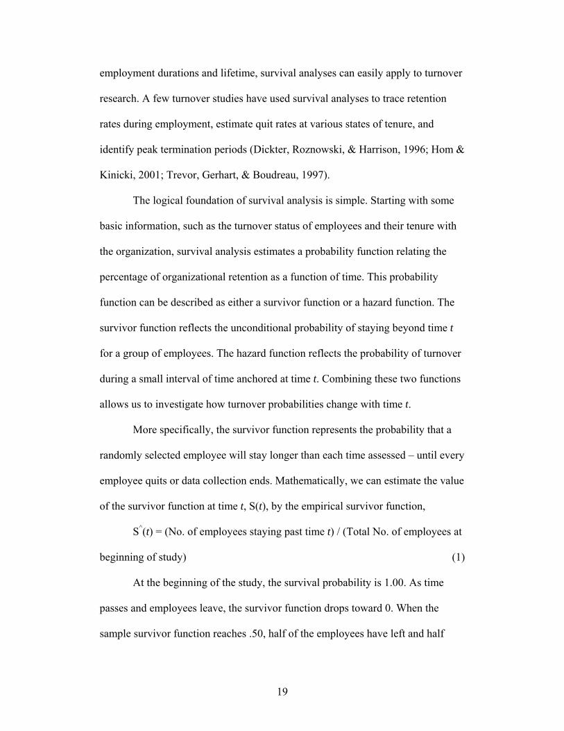
The logical foundation of survival analysis is simple. Starting with some
basic information, such as the turnover status of employees and their tenure with
the organization, survival analysis estimates a probability function relating the
percentage of organizational retention as a function of time. This probability
function can be described as either a survivor function or a hazard function. The
survivor function reflects the unconditional probability of staying beyond time t
for a group of employees. The hazard function reflects the probability of turnover
during a small interval of time anchored at time t. Combining these two functions
allows us to investigate how turnover probabilities change with time t.
More specifically, the survivor function represents the probability that a
randomly selected employee will stay longer than each time assessed – until every
employee quits or data collection ends. Mathematically, we can estimate the value
of the survivor function at time t, S(t), by the empirical survivor function,
S^(t) = (No. of employees staying past time t) / (Total No. of employees at
beginning of study) (1)
At the beginning of the study, the survival probability is 1.00. As time
passes and employees leave, the survivor function drops toward 0. When the
sample survivor function reaches .50, half of the employees have left and half

20
have stayed. When the sample survivor function reaches .25, only one forth of the
employees have stayed and three forth of them have left. The implied assumption
of survivor function is that all employees will leave at certain time t. All survivor
functions have similar shapes of a negatively accelerating extinction curve - a
monotonically decreasing function of time (see Figure 1).
Figure 1. Job tenure survival function.
Different from the survivor function, which describes the probability of
staying, the hazard function effectively captures the distribution of the turnover
risk across time. In the present context, hazard refers to the risk of quitting in each
discrete time period. Based on the estimator of the survivor function, an estimator
for the hazard function at time t is
h^(t) = 1 – [S^(t) / S^(t-1)] (2)

21
In equation 2, h(t) represents the conditional probability that employees will quit
when time = t. Because the hazard function represents the risk of quitting in each
discrete time period, it provides information regarding whether and when turnover
occurs. The hazard function is a probability estimate and thus, it is bounded by 0
and 1. Within these limits, the hazard function can widely vary. The larger the
hazard function, the greater the risk the employees will leave. The lower the
hazard function, the risk of turnover is diminished (See Figure 2).
Figure 2. Job tenure hazard function.
Analysis of survival data typically begins with an examination of the
sample survivor and hazard profiles. Researchers can use a variety of
demographic characteristics of their participants (e.g., part-time/full-time status;

22
minority-majority status) and determine the survival or hazard function separately
for two or more groups. These functions are then compared to determine (a) the
shape of the survivor and hazard function for each group and (b) differences
among the survival and hazard function for the groups. When we compare
survivor or hazard profiles for two or more groups, the characteristic used to
categorize the sample is implicitly treated as a predictor of the survivor or hazard
profile. Thus, profile comparisons provide information regarding the relationship
between turnover and some category variable. For example, Hom and his
colleagues (1993) investigated the impact of realistic job interviews on turnover.
They divided their sample into two subgroups – whether employees had
internship experience or not. They contrasted the survival rates for these two
groups and found that the survival distributions differed significantly between
these two groups (see Figure 3).
If we divide the sample in other ways and treat those divisions as
predictors of turnover, we can investigate the impact of those predictors on
turnover process by comparing survivor or hazard profiles across groups.
However, graphical displays and eye-ball judgments cannot answer complex
research questions. Especially, when the predictor is continuous, we have to
compare cumbersome collection of profiles. Additionally, these methods cannot
explore the effects of several predictors simultaneously and evaluate the influence
of interactions among predictors.
To deal with continuous predictors and several predictors simultaneously,
the proportional hazard models were developed (Singer & Willett, 1991). The

23
Figure 3. Survival Rates as Functions of RJPs and Job Tenure
simplest proportional hazard model consists of one time-invariant predictor. This
simplest proportional hazard model can be present algebraically, like:
Log h(t) = β0 (t) + β1 Predictor1 (3)
In this equation, h(t) is the population hazard profile. β0 (t) refers to the baseline
log-hazard profile and represents the hazard value when the predictor score is zero
and β1 Predictor1 describes the influence of predictor 1 on the hazard profile.
When a hazard model includes multiple time-invariant or time-varying predictors,
more complex models are needed. In such models, time-invariant predictors
describe immutable characteristics of employees, such as gender and race.

24
Time-varying predictors are those variables whose values fluctuate over
time. For example, one possible population hazard model might include time-
invariant Predictor 1 (i.e., race) and time-varying Predictor 2 (i.e., performance)
as follows:
Log h(t) = β0 (t) + β1 Predictor1 + β2 Predictor2 (t) (4)
Where β2 Predictor2 (t) represents that the influence of predictor 2 on turnover
may vary over time.
Survival analysis provides a powerful set of data analytic tools that are
particularly useful in understanding behavioral processes that unfold over time.
Because survival analysis explicitly incorporates time as a variable of interest, it
is more flexible and better able to extract and use information from longitudinal
studies than methods more commonly used on applied psychology. Survival
analysis allows researchers to answer research questions about whether and if
critical events occur. This method is powerful, flexible, and applicable to many
research questions arising in turnover research.
In summary, time and change are two essential characteristic of dynamic
processes. In the previous section, I discussed survival analysis and its ability to
capture the time effect in turnover process. The next section focuses on change
aspect of the dynamic turnover process. When the turnover process and related
variables are described as changing over time, questions such as: (a) “How does
each employee’s turnover function change over time?”; and (b) “Do employees’
trajectories of change vary across leavers and stayers?” can be addressed.
• Growth Modeling
25
Change is inevitable. Change is constant.
- Benjamin Disraeli
The simplest way to know how a person changes over time is to examine
his or her empirical growth plot. An empirical growth plot is a temporally
sequenced graph reflecting the status of some variable over time. These empirical
growth plots can be fitted with various equations to help the researcher summarize
and understand the nature of the change that has occurred in his/her sample over
time. More precisely, separate models are fit to each person’s empirical growth
trajectory. After separate models are estimated for each individual, question such
as: “Does everyone change in the same way?” or “Are the trajectories
significantly different across people or groups?” can be addressed. While many
different models have been developed over the years, Latent Growth Modeling
(GLM) has received increasing attention. To have a better understanding of the
statistical logic of GLM, I will first introduce the Hierarchical Linear Modeling
(HLM) in the following section. GLM can be considered as a structure-equation-
modeling (SEM) version of HLM. The basic statistical equations behind these
methods include (a) to estimate the change trajectory of each individual, which is
considered as the level 1 analysis; and (b) to compare the change trajectories
across all individuals, which is considered as the level 2 analyses.
o Hierarchical Linear Modeling (HLM)
Hierarchical Linear Modeling (HLM) was originally designed to
investigate hierarchically ordered systems. Researchers in sociology (Mason,
Wong, & Entwistle, 1983), education (Burstein, 1980), and organizational

26
behaviors (Mossholder & Bedeian, 1983) have all discussed issues related
hierarchically ordered systems using HLM. The two basic aspects of HLM are the
within-unit (or within-group) differences and the between-unit (or between-group)
differences. HLM has recently gained widespread acceptance as a powerful
approach to the description, measurement, and analysis of longitudinal change
(Bryk & Raudenbush, 1987; Deadrick, Bennett, & Russell, 1997). In the context
of longitudinal research, the central features of HLM are the ability to estimate
within-individual change patterns and the between-individual differences on those
change patterns. In other words, HLM is a multilevel model for change, which
simultaneously fits a pair of equations at two or more levels of analysis. At the
simplest level (referred to as level-1), models that describe the change process of
each person are estimated. At the next level (referred to as level-2) models that
describe how these changes differ across people are fit. Taken together, these two
components form that is know as a multilevel statistical model to address both
within-individual and between-individual questions. .
The level-1 component of HLM represents the change we expect each
member of the population to experience during the time period under study. In
general, we assume that Y it , the observed status of individual i at time t , is a
function of a systematic growth trajectory or growth curve plus random error. The
simplest level-1 model can be represented as:
Y it = π0i + π1i TIME ij + ε it (5)
Where π0i represents an individual i’s true initial status on the dependent variable
(i.e., the value of Y it when TIME ij = 0). Further, π1i represents individual i’s true
27
rate of change during the period under study. Finally, ε it represents that portion of
individual i’s outcome that is unpredicted on occasion j.
The level-2 component of HLM focuses on the relationship between
interindividual differences in change trajectories and employees’ turnover status
(stayers or leavers). The focus of the level 2 model is the growth parameters
captured in the fitted level 1 model. This allows us to test for the predictive power
of level 2 variables to differentiate the “change” process. Specifically, categorical
or continuous level 2 variables (e.g., full-time/part-time; personality) are used to
predict the level 1 model parameters. Mathematically, two related models can be
used to posit the level-2 submodel for interindividual differences in change. One
is for true initial status (π0i) and a second is for true slope of change (π1i):
π0i = γ00 + γ01 Turnover i + ξ 0i (6)
π1i = γ10 + γ11 Turnover i + ξ 1i (7)
In these equations, γ00 and γ10 are the level-2 intercepts, which represent the
population average initial status and slope of change. Further, γ01 and γ11, the
level-2 slopes, provide information about the change trajectories, such as whether
they are increasing over time or decreasing over time. ξ 0i and ξ 1i are the level-2
residuals, which represent those portions of initial status or slopes that cannot be
explained at level-2. The equation (5) demonstrates characteristics of the change
within individuals while the equation (6) and (7) demonstrate the characteristics
of the change between individuals. The set of these three equations are the basic
models of HLM to investigate relationships occurring across multiple levels.
Burstein (1980) has phrased the three equations of HLM under the labels of

28
“intercepts-as-outcomes” and “slope-as-outcomes.” These labels appropriately
describe the conceptual logics of HLM, because the intercepts and slopes
parameters estimated for each individual at level-1 are used as outcome measures
(i.e., dependent variables) in the level-2 model.
o Latent Growth Modeling (LGM)
Similar to HLM, GLM was designed to address questions concerning
intraindividual change (Chan & Schmitt, 2000). As informed earlier, LGM is a
flexible structural equation modeling (SEM) technique that comprehensively
assesses the within-individual changes and between-individual differences in
these changes (Singer & Willett, 2003). By mapping the multilevel model for
change onto SEM, LGM is an alternative approach to capture within-individual
change patterns and it also extends the analytic power of growth modeling.
As same as HLM, LGM represent the longitudinal data by modeling inter-
individual differences in the parameters (i.e., intercept and slope) of intra-
individual changes over time (i.e., individual growth trajectories). The simplest
model is the univariate LGM, which is demonstrated as Figure 4. Two parameters
- intercept (representing initial status) and slope (representing rate of change) –
indicate the intra-individual change pattern over time. Y i1 – Y i3 represent the
three-time measurements of certain constructs, such as antecedents of turnover.
Applying the HLM level-1 model, the intraindividual differences of this LGM
model can be written as:
Y i1 = π0i + π1i TIME 1 + ε i1
Y i2 = π0i + π1i TIME 2 + ε i2

29
Y i3 = π0i + π1i TIME 3 + ε i3 .. (8)
Figure 4 also shows the between-individual differences on the growth
trajectories by comparing the stayers group and the leavers group. Using the HLM
level-2 models, the interindividual differences of this LGM model can be
represented as:
π0i = γ00 + γπ0i + ξ 0i
π1i = γ10 + γπ1i + ξ 1i (9)
As demonstrated in Figure 4, LGM develops a trajectory of change along
each of the focal constructs for each individual across time, through multiple
times of measurements of these constructs (at least three times). More precisely,
each of the longitudinal measurements of a focal construct displays a separate
loading on two latent factors, one defining initial status (i.e., π0i) and one defining
the rate of change (i.e., π1i). The LGM analysis can estimate the means and
variances of the two latent factors (i.e., the intercept – π0i and the slope – π1i). It
can also examine whether these two latent factors are correlated with each other.
Examining each individual’s growth parameters (i.e., π0i and π1i) at the
intraindividual level (by the equations - 8) and at the interindividual level (by the
equations - 9), researchers can investigate the association between individual
growth parameters and the hypothesized variables. For example, in turnover
research, LGM can be used to examine the relationship between individual
performance change and their turnover decisions. The turnover status or turnover
intentions are treated as other latent variables to predict employees’ performance
change patterns.

30
Figure 4. Hypothesized path diagrams of a LGM for turnover
Figure 4 demonstrates the simplest univariate LGM model. Different
univariate LGM models can be combined to form a multivariate LGM, which
allows researchers to investigate the cross-domain associations, such as the
correlations between different change trajectories. More specifically, when the
rate of change of predictor 1(π1i) is correlated with the rate of change of predictor
2 (π’1i), their correlation can be represented and calculated by the multivariate
LGM. For example, previous studies have indicated that the change of
performance and the change of compensation are tied with each other and both of
them are strong predictors of turnover. Multivariate LGM is perfectly suitable for
studying the dynamic relationships between dynamic performance, dynamic
compensation, and turnover.

31
There are two benefits of applying multilevel models to investigate a
dynamic process. First, interindividual differences on the turnover process are
determined by the intraindividual change. In other word, the dependent variables
of level 2 models, π0i and π1i, are the parameters of level 1 model. This allows us
to have a more completed understanding of the turnover process. Second, each
level-2 submodel allows individuals from the same group (either the stayers group
or the leavers group) to have different individual change trajectories. These two
benefits allow researchers to address the following questions of the dynamic
turnover process: (a) the form of the intraindividual change trajectories, (b) the
systematic individual differences at initial status and in the rate of intraindividual
change, (c) the consequences and antecedents of both an individual’s initial status
on the construct of interest and his or her rate of change on that construct across
time, (d) whether there is a relationship between an individual’s initial status and
rate of change on the construct of interest, and (e) whether the change in one
variable is related to the change in another.
LGM has its strong potentials in turnover research, because it overcomes
many of the problems characterizing the traditional methodologies in longitudinal
studies (Chan, 1998; Duncan, Duncan, Strycker, Li, & Alpert, 1999; Lance,
Meade, & Williamson, 2000). Although LGM has much potential for turnover
research, few studies have used this approach to study turnover process (see one
exception: Bentein, Vandenberg, Vandenberghe, & Stinglhamber, 2005). The
present study will have a better opportunity to understand turnover and its
predictors dynamically, by applying multivariate LGM to turnover research.

32
The following section will have a discussion on potential antecedents of a
dynamic turnover process. One important purpose of the next section is to
develop a dynamic turnover process model for further analyses.
Potential Antecedents of a Longitudinal Turnover Process
The aforementioned conceptual models have identified several potential
antecedents of turnover. These antecedents can be classified into two categories:
employee characteristics and organizational/economic contexts. However, given
the disconnection between theory and research design, one has to question the
evidence for a causal relationship between these antecedents and turnover. As
discussed by Mitchell and James (2001), the issue of time and causal relationships
are linked in a complex manner. They suggest that in any investigation of a causal
relationship between two variables, the time when these two variables are
believed to occur and when they are measured are crucial for determining
causality or for providing an unbiased estimate of the magnitude of that
relationship. In other words, researchers need to have theoretical and/or empirical
guides about: (a) when X and Y occur; and (b) when X and Y should be
measured. Without these guides, researchers run the risk of drawing
inappropriate conclusion about the strength, order, and direction of causal
relationships. Thus, it is necessary to include time in turnover studies to
accurately illustrate the relationship between predictors and turnover. In this
section, I will review and discuss the potential antecedents of the dynamic
turnover process. Two major groups of questions will be addressed, which focus
on the time effect and the change effect of the dynamic turnover process.

33
Specifically, the following questions will be discussed: (a) What are the potential
antecedents? (b) Are these antecedents time-invariant? (c) If they are, what are the
changing trajectories of these antecedents? (e) Do those changing trajectories
differ between stayers and leavers? (f) Are these antecedents related to
employment duration? And (g) if they are, what impact they have on the survivor
and hazard functions?
Employee Characteristics
Many reviews of the antecedents and correlates of turnover have appeared
over the years. Employee characteristics, such as demographic and personal
characteristics, job attitudes, performance, promotion opportunities, benefits, and
compensation, have been repeatedly found to predict employment stability (Hom
& Griffeth, 1995; Hulin, Roznowski, & Hachiya, 1985; Mobley, Griffeth, Hand,
& Meglino, 1979; Muchinsky & Tuttle, 1979; Porter & Steers, 1973; Price, 1977;
Steers & Mowday, 1981). A large number of theoretical formulations
demonstrating the turnover process have also underscored the prediction of these
antecedents to turnover decisions, such as Price and Mueller’s (1981) Model of
Turnover, Mobley et al.,’s (1979) Expanded Model of Turnover, and Hulin,
Roznowski, and Hachiya’s (1985) Labor-Economic Model of Turnover.
• Demographic and Personal Characteristics
The demographic and personal characteristics found to predict turnover
decisions include tenure, age, and gender. Previous studies that have used one of
the traditional research designs have indicated that all of these individual
attributes modestly predict turnover, although the magnitude of their relationships

34
with turnover varies. A meta-analysis by Hom and Griffeth (1995) shows the
significant influence of age, sex, and tenure on employee turnover decisions. Hom
and Griffeth (1995) reported that older employees with longer tenure were more
loyal than younger employees with shorter tenure. It was also reported that
women tend to quit more than men. Although age and tenure are treated as time-
variant predictors in this meta-analysis, only the initial age of the participants
could have been used in these studies. In the present study, gender will be treated
as a time-invariant variable whereas age will be allowed to vary across time.
Hypothesis 1a: Female employees will be more likely to quit than male
employees.
Hypothesis 1b: Older employees will be less likely to quit than younger
employees.
• Job Performance
Previous studies on performance and turnover have clearly found a
relationship between these two variables. In multiple meta-analysis studies,
researchers have found a significant negative relationship between performance
and turnover. This repeated finding suggests that lower performers have higher
probabilities to quit (Bycio et al., 1990; McEvoy & Cascio, 1987; Williams &
Livingstone, 1994). Recent research, however, has suggested that the true nature
of this relationship is curvilinear (Trevor et al., 1997; Williams, & Livingston,
1994). Specifically, both high and low performers are more likely to leave an
organization. Unfortunately, most of these studies have rarely investigated this
nonlinear relationship between the changing trajectories of performance and

35
turnover. Interestingly, the issue of the dynamic nature of performance has been
debated for many years (Deadrick, Bennett, & Russell, 1997; Hanges, Schneider,
& Niles, 1990; Hofmann, Jacobs, & Gerras, 1992; Ployhart & Hakel, 1998). Since
prior research has established that performance is an antecedent of turnover and
since prior research has established that performance is dynamic, it seems
reasonable to hypothesize the consequences of dynamic changes in performance
for turnover decisions.
In addition to performance affecting the turnover decision over time, two
empirical studies have found that the relationship between performance and
turnover fluctuates over time (Harrison, Virick, & William, 1996; Sturman &
Trevor, 2001). Given these results, I will treat performance as a time-variant
variable in this study. In particular, I hypothesize that both the initial status of
performance and the nature of the change in performance over time will affect
turnover.
Hypothesis 2a: There will be a curvi-linear relationship between initial
performance and turnover. Specifically, median level performers will
have longer tenure than either high or low performers. Both high
performers and low performers are more like to leave the organization.
Hypothesis 2b: Those individuals that leave and those that stay with the
organization will have different growth trajectories in their performance
over time. Specifically, the slope of performance scores for individuals
that stay with the company will be more positive than the slope of
performance scores for individuals that leave the company.

36
• Compensation
Compensation is commonly believed to be strong antecedents of turnover
by both researchers and practitioners (Gomez-Meija & Balkin, 1992; Milkovich
& Newman, 1993). Unfortunately, very little evidence for this relationship has
been found. This lack of empirical support might be due to the non-dynamic
research designs used in these previous studies. A static design only looks at
salary level and it is possible that level of employees’ salary does not have a
strong influence on turnover decisions because salary levels frequently fall into
acceptable tolerance range when compared to the individual’s desires and market
forces. However, the dynamic perspective emphasizes the change of employees’
salary over time. It is possible that the rate of change will have a strong influence
on employee turnover decisions. In the present study, employees’ compensation
will be treated as a time-variant variable. The slope of compensation change will
also be included.
Hypothesis 3a: There will be a negative relationship between
compensation and turnover. Specifically, employees with higher pay will
have longer employment duration than those with lower pay.
Hypothesis 3b: Employees who leave the organization and those who stay
will have different compensation growth trajectories. Specifically, the
slope of compensation growth trajectories for stayers will be more positive
than the slope of compensation growth trajectories for leavers.
• Promotion

37
Previous research on promotion and turnover has indicated that
promotions exhibit a moderate correlation with turnover (Hom and Griffeth,
1995). More precisely, satisfaction about promotion and perceived opportunities
for promotion modestly predicted turnover whereas actual promotion strongly
predicted turnover decisions. In the present study, I only focus on actual
promotions. Similar to benefits and other types of incentive pay, actual
promotions are events that happen infrequently and only to some employees.
Thus, promotions should be viewed as critical events that influence employees’
assessment of their environment. I therefore hypothesize that it will affect their
turnover decisions.
Previous studies on the influence of promotions on turnover have rarely
adopted a dynamic perspective. Additionally, previous research has not compared
the effect of promotions between those that stay and those that leave an
organization. Thus, it is unclear whether promotions really influence the turnover
process.
Hypothesis 4: Promotions will be related to employment duration.
Specifically, promotions will extend employees’ employment duration.
• General Employees’ Attitudes
Many turnover studies have employees’ general attitudes as antecedents of
resignation. Beyond regular job satisfaction, employees’ general attitudes towards
the organization focuses on employees’ overall attitudes about their organization,
in terms of operations, administrations, climates, and values. As same as job
satisfaction, those attitudes will also affect employees’ turnover decision. A few

38
studies have provided empirical supports for this view. For instance, it has been
found that employees quit their jobs if their experiences disconfirm the
expectations they had about their organizations; they will remain employed if
their experiences confirm their initial expectations (Porter & Steers, 1973;
Wanous et al., 1992).
However, previous studies have rarely investigated the relationship
between employees’ general attitudes and turnover from a longitudinal approach.
That is, employees’ general attitudes toward their organization have been treated
as static variables, although researchers have debated about the instability nature
of attitudes, which are normally considered as exchange ties between employees
and organizational environments. For example, scholars have suggested that
employees’ attitudes toward organizations were calculative attitudes, which is
resulted from employees’ exchange relationship with the organization. In the
present study, employees’ general attitudes will be treated as time-variant
variables. Thus, the hypotheses are addressed below:
Hypothesis 5.1a: Employees with different attitudes will have different
employment duration. Specifically, employees with more positive
attitudes towards the organization will have longer employment tenure
than employees with more negative attitudes.
Hypothesis 5.1b: The attitudes trajectories for employees that stay with an
organization will be more positive than the attitude trajectories of
employees that leave an organization.
• Job Satisfaction

39
Almost all models of turnover have employees’ job satisfaction as
turnover predictors. Low levels of job satisfaction and organizational commitment
are considered as the initial steps along of the turnover process (Hulin,
Roznowski, & Hachiya, 1985; Price & Mueller, 1981; Mobley, 1977; Mobley,
Griffeth, Hand, & Meglino, 1979). Consistent with these theoretical perspectives,
job dissatisfaction and organizational commitment have been found to be related
resignations by many empirical studies (Hom & Griffeth, 1995; Steers &
Mowday, 1981; Porter & Steers, 1973; Price & Mueller, 1986). Three meta-
analysis studies have shown that dissatisfaction employees are more likely to
abandon their present employment than satisfaction employees (Carsten &
Spector, 1987; Hom & Griffeth, 1995; Steel & Ovalle, 1984). For example, in
their meta-analysis of seventy-eight studies covering 27,543 employees, Hom &
Griffeth (1995) found that job satisfaction is significantly correlated (r = -.19)
with resignation.
As same as the discussion about employees’ general attitudes, these
previous studies have rarely examined the longitudinal relationship between job
satisfaction and turnover risks. That is, job attitudes have been treated as static
variables, although researchers have suggested job attitudes are time-variant. In
the present study, job attitudes will be treated as time-variant variables. Not only
the levels of job satisfaction but the change slopes of job satisfaction will be
included into investigation.
Hypothesis 5.2a: Employees with different job satisfaction will have
different employment duration. Specifically, employees with higher job

40
satisfaction will have longer employment tenure than employees with
lower job satisfaction.
Hypothesis 5.2b: The trajectories of employees’ job satisfaction would be
different for stayers and leavers. Specifically, employees who stay with
the organization will have more positive slopes than those who leave.
• Intention to Quit
Intention to quit, conceptually and empirically, has been used as one of the
most important turnover predictors. Different from actual turnover behaviors,
intention to quit presents employees’ psychological attitudes, which may or may
not directly lead to actual turnovers. In many theoretical turnover models,
intention to quit is proposed to be the most direct predictor of turnover behaviors
(Mobley, Griffeth, Hand, & Meglino, 1986; Price & Mueller, 1986; Steers &
Mowday, 1981). Consistent with these theoretical perspectives, intention to quit
has also been found to be closely related to turnover behaviors in multiple
empirical studies. For example, the latest meta-analysis by Griffeth and
colleagues shows that quit intentions remain the best turnover predictors among
all the psychological factors (r = 0.38).
Also, as same as studies on other attitudes predictors, intention to quit is
also considered as being stable over time. In the present study, turnover intention
will also be treated as dynamic variable. That is, the levels of turnover intention,
as well as the slopes of turnover intention, will be included into the analysis to
understand the relations between turnover intentions and turnover behaviors over
time.

41
Hypothesis 5.3a: Employees with different turnover intention will have
different employment duration. Specifically, employees with lower
turnover intention will have longer employment tenure than employees
with higher turnover intention.
Hypothesis 5.3b: The changing trajectories of employees’ turnover
intention would be different for stayers and leavers. Specifically,
employees who stay with the organization will have more negative slopes
than those who leave.
External Economic Contexts
Many of the turnover models have illustrated the importance of the
availability of alternative job opportunities during employees’ turnover decision
process (Hom & Griffeth, 1991; Hulin, Roznowski, & Hachiya, 1985; Mobley,
1977; Mobley, Griffeth, Hand, and Meglino, 1979). It has been suggested that
turnover plans would be contingent on the availability of alternative employment
opportunities. The availability of alternative employment is presented by two
factors in the present study: local unemployment rate and local household income.
Although the aforementioned turnover models have suggested the impact of these
contextual variables on turnover, empirical evidences are limited.
• Local Unemployment Rate
As discussed previously, alternative job opportunities come from within
an organization as well as forces outside the organization (e.g., external economic
conditions). With regard to the external job opportunities, the unemployment rate
is the best indicator. A meta-analysis by Hom and his colleagues (1992) found

42
that unemployment rates moderated the link between employees’ attitudes and
turnover. Gerhart (1987) found that regional unemployment rates moderate
correlations between satisfaction and turnover. Carsten and Spector (1987) also
found that economic expansion facilitates dissatisfied employees to reach their
decision to quit.
Unfortunately, even though the external economic conditions are dynamic,
a dynamic research design has rarely been used to investigate the external
economic conditions to turnover relationship. The present study will treat
unemployment rate as a time-variant variable. Both the economic conditions at
the beginning of the study period and the trajectories of the local unemployment
rate will be included in this study to investigate its dynamic influence on
employees’ turnover decisions.
Hypothesis 6a: Local unemployment rate will affect employees’
employment duration. Employees living in high local unemployment rate
area tend to have longer employment duration than employees living in
low local unemployment rate area.
Hypothesis 6b: The change of local unemployment rate will affect
employees’ turnover decision. The slope of local unemployment rate
change lines for stayers will be more positive than slope of local
unemployment rate change lines for leavers.
• Local Household Income
Local household income, as the other factor to present local economic
situation, is also included in the present study. Local income levels have been

43
used as one important indicator to demonstrate the economic status of the local
area. Although previous research rarely includes local household income in the
turnover studies, local household income, as an important external economical
indicator, is related to turnover risks. That is, employees living in an area with
high local household income are more likely to have higher income, which has
been indicated to extend the employment duration and decrease the turnover risks.
As same as other time-varied predictors, the hypotheses on local household
income are addressed below:
Hypothesis 7a: Local household income will affect employees’
employment duration. Employees living in high household income area
tend to have longer employment duration than employees living in low
household income area.
Hypothesis 7b: The change slopes of local household income will be
different for employees who stay with the organization and those who
leave. The slope for stayers will be more positive than slope for leavers.
Summary
Following the direction of numerous turnover theories and models, the
purpose of this dissertation is to investigate the relationship between multiple
antecedents and employee turnover behaviors. However, different from most
previous turnover research, the present study focuses on the dynamic nature of
turnover process to accurately illustrate the relationship between predictors and
turnover. The time effect and the change effect, which are the two essential
aspects of the dynamic turnover process, are addressed in this study. Two

44
categories of antecedents are included: (a) employee characteristics, including
demographic and personal characteristics (H1), job performance (H2),
compensation (H3), promotion (H4), and job attitudes (H5); and (b) economic
contexts, including local unemployment rate history (H6) and local household
income (H7).
METHODS Participants and Procedure
The initial pool of potential participants consisted of all the employees of a
national wide healthcare company. The primary services that the company
provides include: health care and well-being services, health benefit plans and
services, and pharmaceutical development and consulting services. There was no
sampling issue in this study. All the employees in the organizations were
included. The original data set consisted of 100,877 employees. The data was
collected over a six year period with: N year1 = 49,752, N year 2 = 50,783, N year 3 =
51,074, N year 4 = 50,801, N year 5 = 49,494, N year 6 = 48,407. Of these employees,
17,984 respondents (18%) had data for all six years. The average new hire rate
across the six year period was approximately 19%. The average turnover rate
across six years was approximately 12%. Table 1 shows the number and
percentage of new hires and turnovers for each of the 6 years.
The data used in the present study was obtained from three different
sources: 1) data available from the company’s Human Resource Information
System (HRIS) (e.g., employee compensation level, employee job performance,
and employee demographic information), 2) data obtained from employee surveys

45
(e.g., employee job satisfaction, intention to quit, and general attitudes towards
the organization), 3) data obtained from external archival documents (e.g., local
unemployment rates and local household income). The HRIS data was collected
at the end of each fiscal year. The employee survey was developed and
administrated during the summer of each year. The external archival data was
mainly obtained from the U.S. Bureau of Labor Statistics and the U.S. Census
Bureau.
Table 1. Turnovers and New Hirers by Years
Year 1 Year 2 Year 3 Year 4 Year 5 Year 6 Leavers * 17,495 14,903 13,813 12,516 11,108 9,057 - Voluntary Turnover 6,801 7,105 6,832 5,180 4,078 4,702 - Involuntary Turnover 1,542 1,613 2,951 3,496 3,706 2,909 - Business Turnover 4,382 2,866 1,502 1,330 1,034 68 - Other Turnover 4,770 3,319 2,528 2,510 2,290 1,378 New Hirers 9,255 11,453 9,760 9,952 8,162 7,811 Involuntary Turnover Rate 14% 14% 13% 10% 8% 10% New Hire Rate 19% 23% 19% 20% 16% 16% Total 49,752 50,783 51,074 50,801 49,494 48,407
*Note: The leavers included all four types of turnovers.
The data was obtained from employees that were geographically dispersed
throughout the United States. In the original data set, the average age was 38.8
(SD = 0.50) and the average tenure was 5.3 years (SD = 5.54). Approximately
76% of the respondents were female, 77% were Caucasians, and 96% were
employed full-time. The average annual pay (across the six year period) for the
respondents was $45,416 (SD = $53.925) and the average promotion rate was 8%.
Approximately 29% of employees were rated as high performers and 4% of
employees were rated as low performers.

46
One issue about participants that needs to be addressed when conducting
survival analyses later. This issue focused on how to deal with employees who
were still with the organization when the study was over. Figure 5 illustrates this
issue. As seen in this figure, employees A and C leave the organization during
the study period. The employment duration for these two individuals can be
calculated exactly. However, employees B and D are still with the organization by
the end of the observation point of the study. Calculation of the employment
duration for these individuals is artificially truncated. In reality, employees B and
D have an unknown turnover date. That is, they may leave the organization one
year after the observation period ended. They may leave the organization five
years after the observation period ended or they may leave twenty years after the
observation period ended. Thus, a major issue for turnover studies is deciding
how to portray in the analysis the employment duration of individuals like
employees B and D.
In this study, I applied the approach of treating individuals like employees
B and D as right censored participants. In other words, the data set provides some
information about these individual’s employment duration, but the data set does
not provide this information exactly. For these individuals, their complete
employment duration was cut off (or censored) at the right side of the study
interval.

47
Figure 5. Examples of censoring situation
Measures
Turnover. Turnover information was obtained from the HRIS data file.
Specifically, this file contained the records of each employee’s hire and turnover
(if it occurred) dates. The difference between these two dates (or the time between
being hired and the date of data collection) was used as the measure of duration of
employment. The reason for turnover was also included in this data set.
Specifically, employees’ turnover behaviors were separated into four distinct
categories defined by the organization: voluntary turnover, business decision
turnover, involuntary turnover, and other turnover. Voluntary turnover included
all the employee-initiated turnover behaviors, such as job abandonment, personal
reasons, or return to school. Business decision turnover referred to the turnover

48
behaviors part of the organization reduction in force. Involuntary turnover
behaviors were turnover based employee performance (e.g., attendance or
dishonesty). Other turnover referred to turnover behaviors that were initiated by
ambiguous, unclear, or undefined reasons, such as retirement or death. Consist
with the turnover theories and hypotheses discussed earlier, only voluntary
turnover behaviors were included into the turnover analysis of the present study.
A total of 30,174 individuals, or 30% of the 100,877 respondents, left the
organization voluntarily during the six-year study period. The average
employment duration for those who voluntarily left the organization was 2.58
years (SD = 3.88).
Employment Duration. Beside actual turnover behaviors, employees’
employment duration was also calculated in the present study. All employees
have their entry date. If they left the organization, they would have an exiting
date. If they stayed with the organization until the end of the study, they would be
considered as being right censored. The time between employees’ entry date and
their exiting date was calculated as their employment duration. The employment
duration was recorded by days.
Demographic variables. Demographic variables were obtained from the
HRIS data file. Gender and age were included in the turnover analysis of the
present study. Gender was dichotomized as 1 = female, 2 = male. Age was
measured at employee’s first hiring year. I held age constant at the first hiring
year for this study because the rate of age change is constant across all the
individuals.

49
Job performance. Job performance was also obtained from the HRIS data
file. Job performance was evaluated through the standardized employee
performance appraisal system of the organization. Three categories were used to
rate employee’s job performance: a) Needs improvement, b) Meets expectations,
and c) Exceeds expectations. Across the six years, 20% employees were rated as
“Exceeds expectations”, 69% employees were rated as “Meets expectations”, and
11% employees were rated as “Need improvement”.
Compensation. Employees’ compensation data was obtained from the
HRIS data file. Annual pay rate (full time equivalent) was used to measure the
employee compensation level. Annual pay rate was calculated to permit
meaningful comparisons among both annually-paid employees and hourly paid
employees. I did not include overtime pay, long-term incentive pay, short-term
incentive pay, and other type of payments in this measure. Base pay accounted for
approximately 73 % of individuals’ total income. The average annual pay was
$45,416 with SD = $53.925.
Promotion. Employee promotion records were also obtained from the
HRIS file. Four types of promotion were identified (i.e., regular promotion,
promotion with pay change, planned promotion, and replacement promotion). For
each year, if an employee was promoted (regardless of promotion type), the
promotion variable for that year was coded as 1. Otherwise, the employee’s
promotion variable was coded as 0 – No promotion for that year. The average
promotion rate across six year was 12%. Among employees who had had

50
promotions in the last six years, 78% had one promotion, 18% of had two times of
promotions, and 4% of them had three or more promotions.
Employee attitudes towards the organization. Employees’ attitudes about
the organization were obtained from the organization’s annual employee attitude
survey data. The survey was designed and developed to access employees’
attitudes about the organization regarding four dimensions of: D1 = whether the
organization has clarity and confidence in its direction (3 items), D2 = whether
the organization support employee development and advancement (2 items), D3 =
whether the organization values employees (2 items), and D4 = whether the
organization has good workforce engagement (5 items) (see Table 4 for the
description of the scale items). Each item was a statement of the organization
management. Employees were asked to make judgments on the extent to which
they agree or disagree with these statements (1 = Strongly Agree, 2 = Agree, 3 =
Neither Agree Nor Disagree, 4 = Disagree, 5 = Strongly Disagree, 6 = Don’t
Know/Not Applicable). The reliability of the whole scale across years was α =.87
(αYear4=.86, αYear5=.89, and αYear6=.87). The reliabilities of these four scales over
years were αD1 =.75 (αYear4=.71, αYear5=.79, and αYear6=.73), αD2 =.71 (αYear4=.61,
αYear5=.77, and αYear6=.72), αD3 =.85 (αYear4=.82, αYear5=.88, and αYear6=.83), and
αD4 =.84 (αYear4=.83, αYear5=.87, and αYear6=.82). Respondents indicated
employees’ attitudes towards their organization in terms of its operation,
administration, values, and working environments.
Employee job satisfaction. Besides employees’ attitudes towards the
organization, employees’ job satisfaction was also included in the measurement. It
51
was a single item at the end of the survey: “Considering everything, how would
you rate your overall satisfaction in the Company at the present time?” It was a 5-
point Likert item ranging from 1 (Very satisfied) to 5 (Very Dissatisfied).
Employee intention to quit. In addition, overall intention to quit was
measure by a question on “expect to continue working for the organization” on 6
point scale (1 = Less than 1 year, 2 = 1-3 years, 3 = 3-5 years, 4 = 5-10 years, 5 =
10 years, and 6 = Until Retirement). The list of the statements used to measure job
attitudes are presented in Appendix A.
Unemployment rate. Local unemployment rate was also included in the
present study because it is an important external economic indicator. Local
unemployment rate was obtained from the annual Local Area Unemployment
Statistics reported by the Bureau of Labor Statistics (BLS). Based on the zip
codes of employees’ home addresses, the unemployment rates at the zip-code
level were assigned to each employee. The average local unemployment rate was
4.25% (SD = 1.73).
Local household income. Local household income was obtained from the
annual Income report by the U.S. Census Bureau. The local household income
was linked to each employee by the zip code of the employee’s home address.
The average local household income was $55,312 (SD = $12,220).
Data Analyses
In the present study, different types of variables were included into one
calculation process. The effects of the variables associated with dependent
variables could be influenced by the different quantitative unit they have. In order

52
to facilitate the comparison of the comparative association or prediction strength
across different variables, all continuous variables, except categorical ones, were
standardized at the variable level before conducting the analyses.
Confirmatory factor analyses. All constructs measured by survey scales
(e.g., employee job attitudes) were subject to confirmatory factor analysis (CFA)
to verify the dimensionality of each measure. After specifying a priori factor
structures, CFA matches the observed and theoretical factor structures for a given
data set to determine whether the theoretical structure “fits” the observed data
(Long, 1983).
In the present study, the factor structure for all constructs measured
through multiple items was assessed to verify that a) hypothesized number of
dimensions were obtained and b) the stability of the factor structure was
maintained over time. More specifically, the job attitudes were hypothesized to
measure four subfactors. Each factor consisted of 3 to 5 survey items. Figure 6
contains the conceptual model for the job attitudes construct that was tested.
As stated previously, the fit statistic of CFA results test how well the
conceptual models fit the data. Four fit statistical indicators were used to assess
the empirical support for the hypothesized models. The first indicator used here
was the chi square goodness of fit statistic. The chi square statistic tests the null
hypothesis that there is no statistically significant difference in the observed and
theoretical covariance structure matrices. The chi-square statistic has been
referred to as a "lack of index fit" (Mulaik, James, Van Alstine, Bennet, Lind &
Stilwell, 1989) because a statistically significant result yields a rejection of the fit
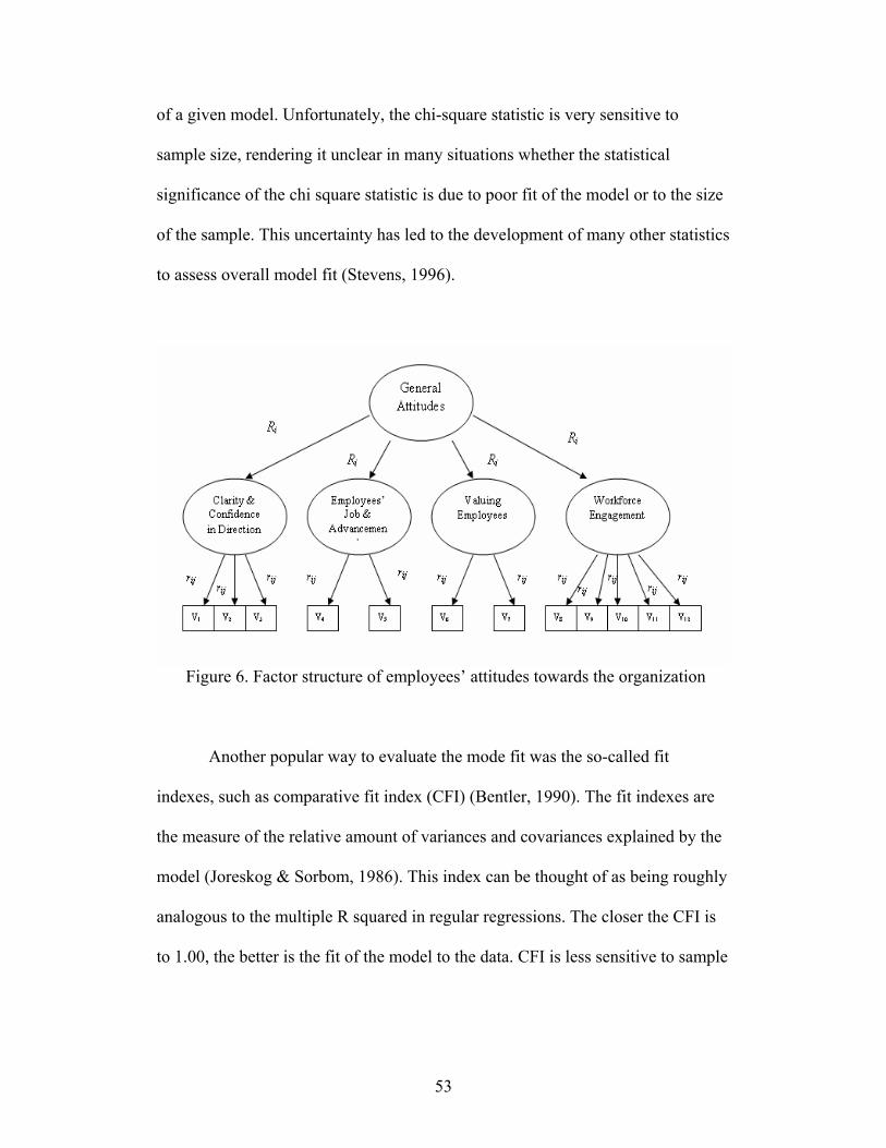
53
of a given model. Unfortunately, the chi-square statistic is very sensitive to
sample size, rendering it unclear in many situations whether the statistical
significance of the chi square statistic is due to poor fit of the model or to the size
of the sample. This uncertainty has led to the development of many other statistics
to assess overall model fit (Stevens, 1996).
Figure 6. Factor structure of employees’ attitudes towards the organization
Another popular way to evaluate the mode fit was the so-called fit
indexes, such as comparative fit index (CFI) (Bentler, 1990). The fit indexes are
the measure of the relative amount of variances and covariances explained by the
model (Joreskog & Sorbom, 1986). This index can be thought of as being roughly
analogous to the multiple R squared in regular regressions. The closer the CFI is
to 1.00, the better is the fit of the model to the data. CFI is less sensitive to sample
54
size than the chi square statistic. The CFI above .90 is considered good (Hu &
Bentler, 1999).
Root mean square error of approximation (RMSEA) was also used in the
present study to evaluate the model fit. According to Hu and Bentler (1999), good
models have an RMSEA of .05 or less. Models whose RMSEA is .10 or more
have poor fit. Proc Calis function of SAS program was used to apply CFA to
analyze the data. Further details of the Proc Calis CFA models used in the present
study are provided in Appendix B.
Survival analyses. Survival analyses were used in the present study to
answer two questions: a) what are the characteristics of people that leave the
organization, and b) for those who leave, when do they exit. In survival analyses,
a hazard function is the main dependent variable. The hazard function showing
the probability of individuals with certain characteristics would leave the
organization as a function of time t (Dickter et al., 1996; Morita et al., 1993;
Singer & Willett, 2003). That is, survival analysis can provide an estimate of the
probability that employees with a particular set of characteristics would leave the
organization at a specific time point.
Two indices were calculated to provide an understanding of how
employee turnover probability changes over time. The first index was the survival
function over the six year study period. As discussed previously, the survival
function refers to the ratio of people staying with the organization at time t over
the number of people who stayed at time t-1. Thus, the survival function
illustrates the relationship between time and survival function: S^(t). The survival

55
curve provides a visual illustration of the relationship between time and survival
probability. The second index was the hazard function and how it changed over
the six year period. The hazard function is the inverse of the survival curve and it
shows the relationship between time and the probability of turnover: h^(t).
Besides providing these two indices of turnover, another primary value of
survival analysis is that it evaluates the relationship between the survival or
hazard functions and other theoretically relevant variables. This function is
especially valuable when it is used to assess the relationship of explanatory
variables to survival duration. Two approaches can be applied to examine this
relationship. The first approach is to compare the survival or hazard curves for
individuals classified by certain variables. If the curves of different groups shape
differently, we say there is a relationship between survival time and the category
variable. For example, Mowday and Lee (1986) compared the survival functions
between cadets having high commitment and those having low commitment. The
second approach applies some form of mathematical modeling, such as the Cox
proportional hazard (PH) approach, to estimate the significant of the relationship.
The Cox PH model provides hazard ratios to quantitatively evaluate the influence
of explanatory variables on survival function. Hazard ratios in survival analysis
were similar to regression coefficients in linear regression or odds ratios in
logistic regression, which could also be understood as the percentage difference in
turnover risk associated with a one-unit difference in the value of the predictor
(Singer & Willett, 2003). A formula can be used to demonstrate this association:
100*(hazard ration - 1). For example, when the hazard ratio for age = 1.0 then the
56
risk of leaving does not change with the change of age. If the hazard ratio for age
= 1.20, then a one unit increase in age results in a 20% increase in risk of leaving.
If the hazard ratio for age = 0.75, then a one unit increase in age results in a 25%
decrease in risk of leaving. Proc PHREG function of SAS program was used to
apply survival analysis on the data. Further details of the specification SAS
program used to conduct the survival analyses in the present study are provided in
Appendix C.
Latent growth modeling. Among all the independent variables, some
variables are constant over time, such as gender. Some variables are changing
with time but are treated as static variables, because: a) the changing is constant
for every individual, such as age, or b) the changing was not considered sensitive
with time, such as promotion. The other variables, such as employees’
compensation, job performance, job attitudes, local unemployment rate, and local
household income, were treated as dynamic variables. That is, the changing
patterns of these variables over time were taken in account when these variables
were used to predict turnover behaviors. Latent growth modeling (LGM) was
used in the present study to examine the patterns of change for all the dynamic
variables over time. As discussed previously, in the present study, LGM were
applied to understand two critical questions related to the dynamic turnover
predictors: a) the form of the intra-individual change trajectories, b) the
systematic inter-individual differences in the intra-individual change trajectories.
Mathematically, two parameter estimates, γ00 and γ10, can be used to answer these
questions. Here, γ00 indicates whether employees have different initial status (or
57
intercept) on their turnover predictors. And, γ10 indicates whether employees have
different change rate (or slope) on their turnover predictors. If both γ00 and γ10 are
significant for a dynamic variable, we can say that the change trajectories of this
variable vary from person to person.
LGM can also be applied to answer anther important question related to
the relationship between dynamic predictors and turnover. That is, LGM can be
used to evaluate whether predicting variables’ changing trajectories are related to
turnover decision. LGM estimates two parameters, γ01 and γ11, to evaluate the
impact of dynamic predictors on turnover behaviors. The first parameter indicates
the initial status of predicting variables that leavers have. The second parameter
indicates the changing rate of turnover predictors that leavers have. If both γ01 and
γ11 are significant, we can say that leavers have different change trajectories of
turnover predictors from people who stay with organization. Proc Mixed function
of SAS program was used to apply LGM to analyze the data. Further details of the
specification SAS program used to conduct LGM analyses for the present study
are provided in Appendix D.

58
Results
Descriptive Statistics
The descriptive statistics for the independent variables across time are
presented in Table 2. The correlation matrix showing the relationships between
variables from year 1 to year 6 are shown in Table 3. Due to the large sample size
(average n across time = 47,836) in the present study, a large number of the
correlations were statistically significant even when the magnitude of these
coefficients were small. The results in Table 4 suggested high reliability of the
measurement of all the variables over time. The range of correlations among same
measurements across years was (0.30, 0.43) (p < .0001). The range of alpha of the
measurements across years was (0.61, 0.89).
The results also indicated that the correlation patterns between variables
were similar across time. Involuntary turnover was found to be correlated with
employees’ attitudes towards the organization, their job performance, and their
annual pay rates. The correlations between employees’ job attitudes towards the
organization and voluntary turnover across years were Year 4 = -.19 (p < .001),
Year 5 = -.18 (p < .001), and Year 6 = -.25 (p < .001). The average correlation
between employees’ job performance and voluntary turnover across years was -
.06 (p < .001), ranging from -.05 (p < .001) to -.07 (p < .001). The average
correlation between employees’ annual pay rate and voluntary turner across years
was -.08, ranging from -.05 (p < .001) to -.13 (p < .001). The involuntary turnover
predictors were also found to be associated with each other. For example, the
averages correlation among employees’ attitudes towards the organization, their

59
performance ratings, and their annual pay rate across years were all significant at
.001 level, ranging from .15 (p < .001) to .17 (p < .001). Additionally, local
unemployment rate was found to be negatively correlated with local household
income.
Confirmatory Factor Analysis (CFA) Results
Employees’ Attitudes towards the Organization. CFA was applied to
evaluate the construct validity of employees’ attitudes measure over time. As
demonstrated by Figure 6, the measurement model of employee attitudes
indicated the 14 job attitude statements loaded on four specific job attitude
factors: “clarity & confidence in direction”, “job and advancement”, “valuing
employees’, “workforce engagement”. In Figure 6, the magnitudes of the loadings
were represented by parameters, rij where the subscript i refers to a particular
latent factor and subscript j refers to a particular item. These four job attitude
factors were hypothesized to load on an overall second order latent factor,
employee overall attitudes. The magnitude of the connections between the
general attitude factor and the four specific attitude factors were indicated by Ri.
Before evaluating the validity of the overall secondary-factor model, the
CFA was first used to test the validity of the four subscales of the overall model.
The CFA results indicated that, except the subscale on “job and advancement”
(CFI = .75, RMSEA = .25), all the other three subscales yielded a robust validity
over time (see Table 4). Specifically, the CFI and RMSEA for subscale on
“clarity & confidence in direction” were .99 and .05; the CFI and RMSEA for
subscale on “valuing employees” were 1.00 and .02; and the CFI and RMSEA for

60
Table 2. Independent Variables Descriptive Statistics over Time – Continuous Variables
Year 1 Year 2 Year 3 Year 4 Year 5 Year 6 Continuous Variables M SD M SD M SD M SD M SD M SD
Age 37.8 56.6 37.5 65.6 38.0 39.5 38.1 39.7 39.2 35.2 39.3 34.0 Tenure 4.46 5.53 4.21 5.46 4.26 5.41 4.43 5.48 4.80 5.60 5.10 5.70 Performance Rating* 2.23 0.51 2.26 0.51 2.18 0.52 2.18 0.54 2.19 0.53 2.12 0.55
Annual Pay Rate $42,473 77,690 $43,239 71,061 $42,384 56,233 $43,526 31,556 $46,639 33,088 $49,245 34,455 Employee Attitudes - - - - - - 1.26 1.39 1.26 1.28 1.60 1.39
Job satisfaction - - - - - - 2.36 0.93 2.34 0.91 2.42 0.94 Intention to quit - - - - - - 1.87 2.28 2.06 2.31 2.36 2.30 Local unemployment rate
3.11 1.52 3.12 1.37 3.71 1.36 4.93 1.64 4.84 1.65 4.55 1.54
Local household income $53,747 $12,284 $53,451 $12,180 $53,213 $12,203 $53,343 $12,380 $53,920 $12,672 $54,554 $12,653
Categorical Variables Percent Percent Percent Percent Percent Percent
Gender – Female 77% 77% 76% 75% 74% 74% Promotion 9% 11% 6% 7% 7% 6% Performance Rating – E 27% 30% 24% 25% 25% 28%
Performance Rating – M 69% 67% 70% 68% 69% 65%
Performance Rating – N 4% 3% 6% 7% 6% 7%
* Performance Rating: “Needs improvement” coded as “1”, “Meets expectations” coded as “2”, and “Exceeds expectations” coded as “3”

61
Table 3. Variables Correlation Matrix
Variables
1 2 3 4 5 6 7 8 9 10 11 12 13 14 15 16 17 18 19 20
1. Gender 1.00 2. Age -0.02 1.00 3. Voluntary Turnover Y1 -0.01 -0.02 1.00 4. Voluntary Turnover Y2 0.00 -0.03 0.12 1.00 5. Voluntary Turnover Y3 -0.02 -0.02 0.12 0.11 1.00 6. Voluntary Turnover Y4 -0.02 0.00 0.13 0.12 0.14 1.00 7. Voluntary Turnover Y5 -0.02 0.03 0.13 0.13 0.14 0.17 1.00 8. Voluntary Turnover Y6 -0.01 0.04 0.10 0.12 0.12 0.15 0.14 1.00 9. Performance Rating Y1 0.02 0.01 -0.05 -0.03 -0.02 0.00 0.00 0.02 1.00 10. Performance Rating Y2 0.02 0.00 -0.01 -0.06 -0.03 -0.01 0.00 0.02 0.63 1.00 11. Performance Rating Y3 0.00 0.01 0.00 0.00 -0.07 -0.04 0.01 0.00 0.26 0.37 1.00 12. Performance Rating Y4 0.00 0.01 -0.01 0.01 0.00 -0.06 -0.03 -0.01 0.19 0.22 0.41 1.00 13. Performance Rating Y5 0.00 0.00 0.01 0.01 0.01 0.00 -0.05 -0.03 0.15 0.17 0.22 0.41 1.00 14. Performance Rating Y6 0.00 -0.01 0.02 0.02 0.01 0.00 0.01 -0.06 0.15 0.17 0.20 0.26 0.42 1.00 15. Pay Y1 0.11 0.00 -0.05 -0.04 -0.02 -0.01 0.01 0.03 0.15 0.15 0.10 0.09 0.09 0.08 1.00 16. Pay Y2 0.12 0.00 -0.01 -0.03 -0.04 -0.01 0.00 0.03 0.15 0.16 0.12 0.11 0.10 0.09 0.72 1.00 17. Pay Y3 0.15 0.01 -0.01 -0.02 -0.07 -0.05 -0.02 0.00 0.18 0.17 0.16 0.14 0.11 0.11 0.68 0.95 1.00 18. Pay Y4 0.28 0.03 -0.02 -0.02 -0.05 -0.13 -0.06 -0.02 0.20 0.19 0.18 0.17 0.14 0.13 0.37 0.57 0.68 1.00 19. Pay Y5 0.30 0.04 -0.02 0.00 -0.03 -0.05 -0.10 -0.04 0.20 0.19 0.18 0.17 0.15 0.14 0.79 0.78 0.92 0.96 1.00 20. Pay Y6 0.30 0.04 0.00 0.02 0.00 -0.01 -0.03 -0.08 0.20 0.19 0.18 0.17 0.15 0.17 0.79 0.73 0.88 0.91 0.94 1.00 21. Promotion Y1 0.01 -0.01 -0.07 0.01 0.01 0.00 0.00 0.00 0.12 0.09 0.04 0.05 0.05 0.04 -0.01 -0.01 0.00 0.02 0.03 0.03 22. Promotion Y2 0.01 0.00 -0.02 -0.08 -0.02 0.01 0.02 0.01 0.08 0.14 0.09 0.06 0.05 0.04 -0.03 0.00 0.00 0.02 0.02 0.02 23. Promotion Y3 0.00 -0.01 -0.01 -0.01 -0.06 -0.01 0.02 0.00 0.02 0.05 0.13 0.05 0.04 0.05 -0.03 -0.02 0.00 0.01 0.01 0.02 24. Promotion Y4 0.00 -0.01 -0.01 -0.01 -0.02 -0.06 -0.01 0.00 0.01 0.02 0.06 0.19 0.08 0.05 -0.03 -0.04 -0.03 0.01 0.00 0.00 25. Promotion Y5 0.00 -0.01 0.00 0.01 -0.01 -0.01 -0.05 -0.02 0.02 0.04 0.03 0.10 0.21 0.08 -0.04 -0.04 -0.04 -0.03 0.01 0.01 26. Promotion Y6 0.01 -0.03 0.00 0.00 -0.01 0.00 -0.01 -0.06 0.01 0.02 0.02 0.04 0.07 0.19 -0.03 -0.02 -0.03 -0.03 -0.02 0.02 27. Job Attitudes Y4 -0.01 0.05 0.00 -0.01 -0.05 -0.19 0.04 0.01 0.02 0.02 0.06 0.08 0.01 -0.01 -0.08 -0.05 -0.02 0.03 -0.02 -0.01 28. Job Attitudes Y5 0.02 0.05 -0.01 -0.01 -0.01 -0.04 -0.18 0.00 0.00 0.01 0.02 0.07 0.09 0.03 -0.08 -0.05 -0.03 0.01 0.06 0.02 29. Job Attitudes Y6 -0.01 0.05 0.00 -0.01 -0.01 -0.01 -0.04 -0.25 0.00 0.00 0.01 0.03 0.05 0.07 -0.09 -0.07 -0.06 -0.03 0.00 0.03 30. Unemployment Rate Y1 -0.07 -0.01 0.01 0.01 0.00 0.00 -0.02 -0.02 -0.05 -0.04 -0.03 -0.01 0.01 0.00 0.02 -0.02 -0.04 -0.13 -0.12 -0.14 31. Unemployment Rate Y2 -0.07 0.00 -0.02 0.01 0.01 0.01 -0.01 -0.02 -0.05 -0.05 -0.04 -0.02 0.00 -0.01 0.01 -0.04 -0.06 -0.14 -0.14 -0.16 32. Unemployment Rate Y3 -0.07 -0.01 -0.02 -0.01 0.02 0.01 0.00 -0.02 -0.08 -0.07 -0.05 -0.03 -0.01 -0.02 0.00 -0.05 -0.06 -0.14 -0.14 -0.16 33. Unemployment Rate Y4 -0.05 -0.01 -0.02 -0.01 -0.01 0.03 0.02 -0.01 -0.07 -0.06 -0.03 -0.03 -0.02 -0.03 0.00 -0.05 -0.06 -0.10 -0.10 -0.11 34. Unemployment Rate Y5 -0.04 -0.01 -0.02 -0.01 -0.02 -0.01 0.01 -0.01 -0.05 -0.05 -0.03 -0.02 -0.01 -0.03 -0.08 -0.07 -0.09 -0.08 -0.07 -0.09 35. Unemployment Rate Y6 -0.03 0.00 -0.01 -0.01 -0.01 -0.01 -0.01 -0.02 -0.06 -0.05 -0.04 -0.02 -0.02 -0.04 -0.10 -0.08 -0.09 -0.09 -0.08 -0.08 36. Household Income Y1 0.09 0.01 0.00 0.03 -0.01 0.00 0.00 0.02 0.06 0.08 0.05 0.04 0.03 0.02 0.06 0.10 0.12 0.26 0.26 0.25 37. Household Income Y2 0.10 0.01 0.01 0.02 -0.04 -0.02 0.00 0.02 0.06 0.08 0.06 0.05 0.04 0.03 0.06 0.10 0.13 0.27 0.27 0.25 38. Household Income Y3 0.09 0.01 0.02 0.02 -0.04 -0.04 -0.01 0.02 0.07 0.08 0.07 0.07 0.05 0.04 0.07 0.12 0.14 0.28 0.28 0.26 39. Household Income Y4 0.10 0.02 0.02 0.03 0.02 -0.05 -0.03 0.01 0.08 0.09 0.08 0.08 0.05 0.04 0.08 0.16 0.19 0.29 0.29 0.26 40. Household Income Y5 0.11 0.02 0.03 0.03 0.02 0.01 -0.04 0.01 0.08 0.10 0.09 0.08 0.05 0.05 0.24 0.23 0.27 0.29 0.29 0.26 41. Household Income Y6 0.10 0.03 0.03 0.04 0.02 0.02 0.02 0.01 0.08 0.09 0.09 0.07 0.04 0.05 0.23 0.22 0.26 0.27 0.27 0.26
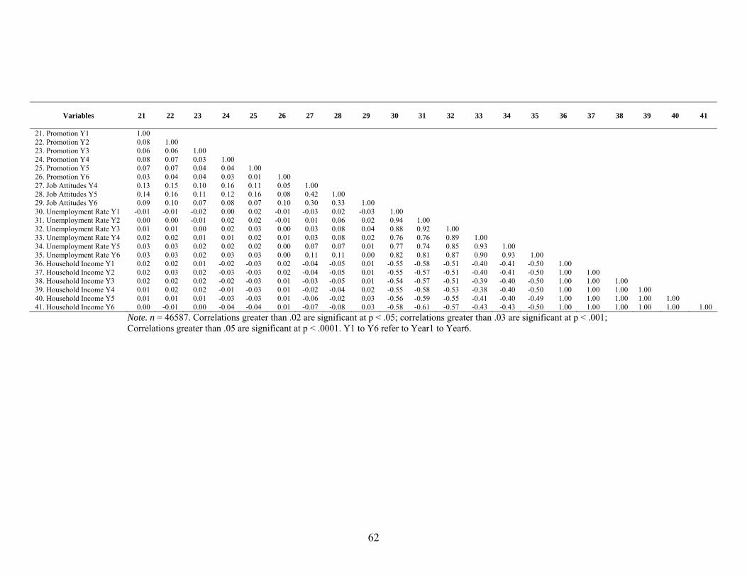
62
Note. n = 46587. Correlations greater than .02 are significant at p < .05; correlations greater than .03 are significant at p < .001; Correlations greater than .05 are significant at p < .0001. Y1 to Y6 refer to Year1 to Year6.
Variables
21 22 23 24 25 26 27 28 29 30 31 32 33 34 35 36 37 38 39 40 41
21. Promotion Y1 1.00 22. Promotion Y2 0.08 1.00 23. Promotion Y3 0.06 0.06 1.00 24. Promotion Y4 0.08 0.07 0.03 1.00 25. Promotion Y5 0.07 0.07 0.04 0.04 1.00 26. Promotion Y6 0.03 0.04 0.04 0.03 0.01 1.00 27. Job Attitudes Y4 0.13 0.15 0.10 0.16 0.11 0.05 1.00 28. Job Attitudes Y5 0.14 0.16 0.11 0.12 0.16 0.08 0.42 1.00 29. Job Attitudes Y6 0.09 0.10 0.07 0.08 0.07 0.10 0.30 0.33 1.00 30. Unemployment Rate Y1 -0.01 -0.01 -0.02 0.00 0.02 -0.01 -0.03 0.02 -0.03 1.00 31. Unemployment Rate Y2 0.00 0.00 -0.01 0.02 0.02 -0.01 0.01 0.06 0.02 0.94 1.00 32. Unemployment Rate Y3 0.01 0.01 0.00 0.02 0.03 0.00 0.03 0.08 0.04 0.88 0.92 1.00 33. Unemployment Rate Y4 0.02 0.02 0.01 0.01 0.02 0.01 0.03 0.08 0.02 0.76 0.76 0.89 1.00 34. Unemployment Rate Y5 0.03 0.03 0.02 0.02 0.02 0.00 0.07 0.07 0.01 0.77 0.74 0.85 0.93 1.00 35. Unemployment Rate Y6 0.03 0.03 0.02 0.03 0.03 0.00 0.11 0.11 0.00 0.82 0.81 0.87 0.90 0.93 1.00 36. Household Income Y1 0.02 0.02 0.01 -0.02 -0.03 0.02 -0.04 -0.05 0.01 -0.55 -0.58 -0.51 -0.40 -0.41 -0.50 1.00 37. Household Income Y2 0.02 0.03 0.02 -0.03 -0.03 0.02 -0.04 -0.05 0.01 -0.55 -0.57 -0.51 -0.40 -0.41 -0.50 1.00 1.00 38. Household Income Y3 0.02 0.02 0.02 -0.02 -0.03 0.01 -0.03 -0.05 0.01 -0.54 -0.57 -0.51 -0.39 -0.40 -0.50 1.00 1.00 1.00 39. Household Income Y4 0.01 0.02 0.02 -0.01 -0.03 0.01 -0.02 -0.04 0.02 -0.55 -0.58 -0.53 -0.38 -0.40 -0.50 1.00 1.00 1.00 1.00 40. Household Income Y5 0.01 0.01 0.01 -0.03 -0.03 0.01 -0.06 -0.02 0.03 -0.56 -0.59 -0.55 -0.41 -0.40 -0.49 1.00 1.00 1.00 1.00 1.00 41. Household Income Y6 0.00 -0.01 0.00 -0.04 -0.04 0.01 -0.07 -0.08 0.03 -0.58 -0.61 -0.57 -0.43 -0.43 -0.50 1.00 1.00 1.00 1.00 1.00 1.00

63
subscale on “workforce engagement” were .96 and .08. Thus, the subscale on “job
and advancement” was deleted from the over model, because of its low construct
validity over time. The CFA was applied to a three-factor secondary factor model.
The CFA results of the overall model were also shown on Table 4. The
correlation matrix for the 10 items was used in this analysis. The results using the
unstandardized correlation matrix did not differ substantially from the
standardized correlation matrix, thus, only the results using the standardized
correlation matrix were reported. A multigroup CFA was used to evaluate the
validity of the overall factor model over time.
Although the Chi-square tests for the multigroup secondary three-factor
model were significant (x2= 13779.69, df = 32, p < .001), which indicated a poor
fit of the theoretical model. However, The CFI was .90 and RMSEA was .06 for
the proposed three-factor model, which suggested that the proposed secondary
three-factor model had a acceptable fit for the observed data cross years.
The standardized parameter estimates for the associations between factors
and items (Ri and rij) were also presented in Table 4. As presented on the table,
items loadings ranged from.60 to .85. All the loadings were statically significant
(p < .001). There were also significant associations between secondary factor and
lower level factors. The average association between clarity & confidence in
direction and the secondary factor was .98 (R1 = .99, .98, .96 respectively, p <
.001). The average association between valuing employees and the overall factor
was .93, ranging from .88 (p < .001) and .98 (p < .001). And, the average
association between workforce engagement and the general factor was .94,

64
Table 4. Multigroup CFA Results for Employee Attitude Measurements over Time
Overall Model Cross Years Goodness-of-Fit Results for the overall model cross years
x2(df) 13779.69(32)*** CFI .90
RMSEA .06 Standardized estimates of associations for each year Year 4 Year 5 Year 6 R1: Clarity & Confidence in Direction 0.99*** 0.98*** 0.96*** R2: Valuing Employees 0.88*** 0.92*** 0.98*** R3: Workforce Engagement 0.92*** 0.97*** 0.94***
Factor 1: Clarity & Confidence in Direction Goodness-of-Fit Results for this factor
x2(df) 538.08(8)*** CFI 0.99
RMSEA 0.05 Standardized estimates of associations for each year Year 4 Year 5 Year 6 - The company has a clear sense of direction 0.70*** 0.74*** 0.71*** - The changes of the company make us a better company. 0.65*** 0.70*** 0.68*** - Senior management’s actions consistent with their words. 0.68*** 0.79*** 0.69***
Factor 2: Valuing Employees Goodness-of-Fit Results for this factor
x2(df) 7.66(1)** CFI 1.00
RMSEA 0.02 Standardized estimates of associations for each year Year 4 Year 5 Year 6 - Senior management demonstrates that employees are important to the success of the business. 0.86*** 0.85*** 0.78***
- The company takes a genuine interest in the well-being of its employees. 0.80*** 0.77*** 0.70***
Factor 2: Workforce Engagement Goodness-of-Fit Results for this factor
x2(df) 5249.288(31)*** CFI 0.96
RMSEA 0.08 Standardized estimates of associations for each year Year 4 Year 5 Year 6 - Overall, the company is an effectively managed, well-run business. 0.60*** 0.72*** 0.60***
- I feel proud to work for the company. 0.83*** 0.87*** 0.82*** - Overall, the company is a good place to work, compared to other organizations I know about. 0.73*** 0.79*** 0.71***
- I am enthusiastic about my future with the company as a place to work and develop my skills. 0.75*** 0.79*** 0.76***
- My work gives me a feeling of personal accomplishment. 0.60*** 0.60*** 0.60*** Note. *** p < .001, ** p < .01. CFI: Bentler's Comparative Fit Index. RMSEA: Root Mean Square Error of Approximation.

65
ranging from .92 (p < .001) and .97 (p < .001). Additionally, the standardized
model parameter estimates indicated that the magnitudes of the links within the
conceptual model held stable over time.
Overall, the CFA results provided support for the job attitude
measurement model. The measurement on employees’ attitudes towards the
organization had strong construct validity and its validity was stable across time.
Thus, the employee attitudes data, which would be used in further analyses, were
valid.
Survival Analysis Results
Prior to presenting the results of the survival analysis, it is important for
the reader to remember two critical issues about survival analysis. First, as
discussed in the introduction section of this dissertation, I examined the predictive
power of 11 variables in this study. I used univariate survival models to examine
the effect of each variable on employment duration. Secondly, there were two
options to include participants in the survival analysis. The first way was only
including employees hired during the six-year study period in the survival
analysis. While this sample provided an accurate estimate of the relationship
between predictors and turnover for the six-year study period, information from
employees with employment duration greater than 6 years was systematically
ignored in this sample. The second option was including all the employees and
allowed an evaluation of the relationship between the predictors and employee
duration for a greater range of employment duration data (time > 6 years). It
should be noted, however, that the survival function and hazard function estimates

66
based on this second sample were biased, because it does not include employees
who left the organization before the study period. Thus, to have a more accurate
estimation of the survival and hazard function, the present study only included
employees hired during the six-year study period. The results from the univariate
survival analyses were presented in Table 6. Interpretation and explanation of the
results were addressed in the following section.
As presented on Table 5, the first column was the estimated parameters for
the associations between predictors and turnover risk. The second and their
columns demonstrated the significant levels of the association: Standard error and
Chi-square. The last column was hazard ratio, representing the percentage
difference in turnover risk associated with a one-unit difference in the value of the
predictor. The results shown on Table 6 suggested that there were significant
association between all the predictors and employment duration (p < .0001).
Among the predicting variables, age, employee attitudes towards the organization,
employee annual pay rates, promotion, and their intention to quit and job
satisfaction had strong impacts on turnover risk. There were a significant but
moderate association between employees’ employment duration and their
performance ratings, their gender, and their local economical conditions.
Hypothesis 1a. As discussed previously, hypothesis 1a predicted that
female employees will be more like to leave the organization than male
employees. The results of the univariate survival analysis supported hypothesis
1a. The univariate survival model for gender and turnover examined the survival
functions and the hazard functions. The estimate parameter for the relationship

67
Table 5. Univariate Survival Models Predicting Employment Duration
Parameter Estimate
Standard Error Chi-Square Hazard Ratio
Gender -0.10 0.01 55.38*** 0.90 Age -2.08 0.03 5958.21*** 0.12 Performance Rating -0.34 0.02 568.01*** 0.71 Annual Pay Rate -0.97 0.02 3237.41*** 0.38 Promotion -0.81 0.01 3101.22*** 0.44 Employee Attitudes -1.06 0.01 9523.20*** 0.35 Job Satisfaction -0.43 0.02 457.21*** 0.47 Intention to Quit 1.47 0.02 7277.71*** 1.77 Local Unemployment Rate -0.13 0.01 975.61*** 0.88 Local Household Income -0.10 0.01 215.06*** 0.90
Note. All the continuous predictors were standardized prior to analysis. *** p < .0001. All the variables were standardized before conducting the survival analyses.
between gender and turnover was -.10 (χ2 (1) = 55.38; p < .0001). The result
indicated that, with only this single predictor in the survival model, there was a
substantial impact of gender on turnover risk. Since female was coded as 1 and
male was coded as 2, the results show females were more likely to quit than
males. The hazard ratio of gender based on the new-hiring sample was .90.
Specifically, the turnover risk for females was 10 % higher than for males (see
Figure 7 and Figure 8).
Figures 7 and 8 show that, males had a higher survival rate and lower
hazard rate than females over the 6 year study period. More specifically, from
Figure 7, we can also see that 50% of males quit after 4 years whereas 50% of
females quit over 5 years. From Figure 8, we can see that employees face the
highest turnover risk during their first three years in the organization. Thus, the
hypothesis 1a was supported by the survival analysis results.

68
Figure 7. Univariate survival function estimate by gender

69
Figure 8. Univariate hazard function estimate by gender

70
Hypothesis 1b. As addressed previously, hypothesis 1b predicted that
older employees will be less likely to quit than younger employees. The results of
the univariate survival analysis supported this hypothesis. Although employee age
is changing over the length of the study period, I treated age as a static variable by
only using employee’s age at hire. Since the rate of change in age is a constant
for employees in my study, the rate of change in age provides no meaningful
explanatory variance in the survival analysis. Thus, the only meaningful age
difference between employees was the age at hire.
With age as the only predictor in the survival model, a significant negative
relationship between age and employee turnover was found. The estimate
parameter for the relationship between age and turnover was -2.08 (χ2 (1) =
5958.21; p < .0001). The hazard ratios were .12. In other words, a one
standardized deviation increase in age resulted in an 88% decrease in turnover
risk.
To further demonstrate the differences between employees of different
ages, I categorized age into two levels: younger employees (age < 38) versus
older employees (age >= 38). The survival and hazard curves for younger
employees and older employees are shown in Figure 9 and Figure 10. These
figures show that younger employees tend to have a higher turnover risk than do
older employees.
As demonstrated on Figure 9, for employees younger than 38 years old,
approximately 50% leave the organization after 3.5 years of employment.
However, approximately 50 % of the employees 38 years or older would not leave

71
Figure 9. Univariate survival function estimate by age
Note: Employees were split into two groups according to the median age (38 years old): (1) employees older than 38 years and (2) employees younger than 38 years.

72
Figure 10. Univariate hazard function estimate by age
Note: Employees were split into two groups according to the median age (38 years old): (1) employees older than 38 years and (2) employees younger than 38 years.

73
the organization during the six-year study period. It should be noted, although
younger employees had a greater likelihood of leaving than did older employees,
both groups exhibited the same change pattern in the hazard function across time
(see Figure 10). As a conclusion, hypothesis 1b was supported by the results.
Hypothesis 2a. As discussed previously, I performed separate analyses
with job performance. In one set of analyses, job performance was treated as a
stable trait (i.e., an individual’s performance was averaged over time). In the
second set of analysis, a latent growth model was applied to determine whether
change in job performance corresponded with changes in turnover risk over time.
To evaluate hypothesis 2a, the first set of analyses were conducted.
Hypothesis 2a stated that there was a curvi-linear relationship between
performance ratings and turnover behaviors. That is, median level performers will
have longer tenure than either high or low performers. However, the results did
not support the curvi-linear argument. A linear relationship between performance
ratings and turnover was found from the results. The estimated parameter for the
relationship between age and turnover was -0.34 (χ2 (1) = 568.01; p < .0001). The
hazard ratios were .71. In other words, one unit increase in employee job
performance ratings results in a 29% decrease in their turnover risk. More
specifically, employees rated, on average, as Needs Improvement had a 29%
higher turnover risk than employees rated, on average, as Meets Expectations.
These employees had a 29% higher turnover risk than did employees rated, on
average, as Exceeds Expectations. The survival and hazard curves for employees
with different performance ratings were presented in Figure 11 and Figure 12.

74
Figure 11. Univariate survival function estimate by performance rating

75
Figure 12. Univariate hazard function estimate by performance rating
76
The same relationship between performance ratings and turnover risk can
be seen in the survival function and the hazard function figures. As demonstrated
on Figure 11, approximately 50% of the low performers quit by 3.5 years,
whereas approximately 50% of the median performers left the organization by 5.5
years. Finally, approximately 60% of the high performers remained with the
organization by the end of the sixth year of the study. As demonstrated on Figure
12, the turnover risk for employees of different performance levels held stable
over time. Higher performers always had lower turnover risk than did median or
lower level performers. Thus, the hypothesis 2a was not supported by the survival
analysis results. A linear, instead of a curvi-linear, relationship between
performance ratings and turnover risk was found in the present study.
Hypothesis 3a. Compensation was also treated as a longitudinal variable.
Hypothesis 3a focused on the different survival patterns of employees with
different pay levels and Hypothesis 3b focused on the relationship between the
changing trajectories of compensation and turnover behaviors. Thus, following
the approach that I took previously, in the survival analysis, I used the average
level of compensation across the study’s time period to test hypothesis 3a. In the
later analysis – the latent growth modeling analysis, I would test whether change
in compensation over the years was related to change in turnover risk.
Hypothesis 3a predicted a negative relationship between employees’
annual pay rates and their turnover risk. The results from the univariate model
supported this hypothesis. The estimated parameter was -.97 (χ2 (1) =3237.41; p <
.0001), which indicated that annual pay rates had significant negative impact on

77
Figure 13. Univariate survival function estimate by compensation level
Note: Employees were split into three groups according to their pay: a) “Employee with High Pay” (Annual pay rate >= 75 percentile), b) “Employee with Median Pay” (Annual pay rate between 75 percentile and 25 percentile), and c) “Employee with Low Pay” (Annual pay rate <= 25 percentile).

78
Figure 14. Univariate survival function estimate by compensation level
Note: Employees were split into three groups according to their pay: a) “Employee with High Pay” (Annual pay rate >= 75 percentile), b) “Employee with Median Pay” (Annual pay rate between 75 percentile and 25 percentile), and c) “Employee with Low Pay” (Annual pay rate <= 25 percentile).

79
turnover risk. The hazard ratios were .43. That is, one standardized deviation
increase in pay decreased the turnover risk by 50% to 60%. To illustrate the effect
of compensation on the survival and hazard function, I trichotomized the data by
employee average annual pay. The high pay group was defined as employees in
the top quartile of pay. The low pay group was defined as employees in the
bottom quartile of pay. The mid-range pay group was defined as employees in
the middle two quartiles of pay. The survival and hazard curves for employees
with different pay rates were presented on Figure 13 and Figure 14.
As demonstrated on Figure 13, approximately 50% of the low pay group
quit after 1.5 years of employment. For the median pay group, 50% of quit after
4.5 years. Finally, for the high pay group, only 35% left over the 6 year period of
the study. From Figure 14, we could see that the risk of turnover for different
performers held stable across the six years. And higher performance always had
lower risk to quit than median and low performers. Thus, hypothesis 3a was
supported by the results.
Hypothesis 4. Promotion was hypothesized to be related to employment
duration. Specifically, promotions would extend employees’ employment
duration. As discussed previously, the total number of promotions during the six-
year study period was used as the value of promotion. The results from univariate
survival model indicated a substantial impact of promotion on employment
duration. The estimate parameter for the relationship between promotion and
turnover risk was -0.81 (χ2 (1) = 3101.22; p < .0001). The hazard ratios from the

80
Figure 15. Univariate survival function estimate by promotion
Note: Employees were split into three groups based on the times of promotion in the study period: (1) employees with more than 1 time of promotion, (2) employees with 1 time of promotion, and (3) employees with no promotion.
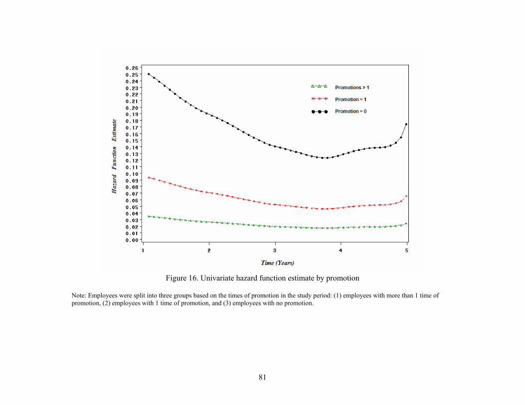
81
Figure 16. Univariate hazard function estimate by promotion
Note: Employees were split into three groups based on the times of promotion in the study period: (1) employees with more than 1 time of promotion, (2) employees with 1 time of promotion, and (3) employees with no promotion.

82
univariate model were .44, which indicated that each instant of promotion would
reduce employees’ turnover risk by about 50% to 60%.
The survival and hazard curves for employees with different promotion
rates were presented on Figure 15 to Figure 16. As can be seen in Figure 15, about
50% of the employees who did not have a single promotion during the six-year
study period would quit within 3 years of employment. Employees who received
at least one promotion stayed with the organization throughout the entire study
period. As demonstrated as Figure 16, the hazard function also show that
employees without promotion had much higher risk to leave than employees with
one time or multiple times of promotion. Overall, the hypothesis 4 was supported.
Hypothesis 5.1a. Employees’ attitudes towards the organization were
obtained from employee surveys across years in this study. This enabled me to
analyze the survey data as a longitudinal variable. Following my procedure,
however, I averaged survey scores across years in this initial stage to evaluate
hypothesis 5.1.a., because this hypothesis focused on the different survival
functions between employees with different attitudes towards the organization.
The results from the univariate survival model indicated that employees’
attitudes towards their organization had a significant impact on their employment
duration. The estimated parameter between attitudes and turnover risk was -1.06
(χ2 (1) =9523.20; p < .0001). The hazard ratio from the univariate model was .35,
which indicated that one standardized deviation increase in employees’ attitudes
about their organization resulted in a 65% decrease in their turnover risk.

83
Figure 17. Univariate survival function estimate by employees’ attitudes
Note: Employees were split into three groups according to their attitudes: a) “Employee with Positive Attitudes” (Attitudes scores >= 75 percentile), b) “Employee with Neutral Attitudes” (Attitudes score between 75 percentile and 25 percentile), and c) “Employee with negative Attitudes” (Attitudes score <= 25 percentile).

84
Figure 18. Univariate hazard function estimate by employees’ attitudes
Note: Employees were split into three groups according to their attitudes: a) “Employee with Positive Attitudes” (Attitudes scores >= 75 percentile), b) “Employee with Neutral Attitudes” (Attitudes score between 75 percentile and 25 percentile), and c) “Employee with negative Attitudes” (Attitudes score <= 25 percentile).

85
To have a clearer display of the relationship between employee attitudes
and survival function, employees were split into three groups according to their
attitudes: a) “Employee with Positive Attitudes, b) “Employee with Neutral
Attitudes”, and c) “Employee with negative Attitudes” (see Figure 17 and Figure
18). As demonstrated on Figure 17, approximately 60% of the employees with
low job satisfaction leave the organization before the end of two years of
employment. The turnover risk was 22% and 9% for employees with neutral and
positive levels of job satisfaction, respectively. From Figure 18, we could see that
the turnover risk for employees with negative overall attitudes was much higher
than other employees. The turnover risk for employees with positive and neutral
overall attitudes were similar and stable over time Overall, the hypothesis 5.1.a
was supported.
Hypothesis 5.2a. This hypothesis predicted that employees with different
job satisfaction would have different employment duration. Specifically,
employees with higher job satisfaction would have longer employment tenure
than employees with lower job satisfaction. As same as the discussed approach,
the average scores of job satisfaction across years were used to test this
hypothesis.
The results from the univariate survival model indicated a significant
negative association between employees’ job satisfaction and their turnover risk.
The association parameter between satisfaction and turnover risk estimated by the
univariate survival model -.43 (χ2 (1) =457.21; p < .0001). The hazard ratios from

86
Figure 19. Univariate survival function estimate by job satisfaction
Note: Employees were split into three groups according to their job SAT: a) “Employee with High Job SAT” (Job satisfaction scores >= 75 percentile), b) “Employee with Median Job SAT” (Job satisfaction scores between 75 percentile and 25 percentile), and c) “Employee with Low Job SAT” (Job satisfaction scores <= 25 percentile).

87
Figure 20. Univariate hazard function estimate by overall satisfaction
Note: Employees were split into three groups according to their job SAT: a) “Employee with High Job SAT” (Job satisfaction scores >= 75 percentile), b) “Employee with Median Job SAT” (Job satisfaction scores between 75 percentile and 25 percentile), and c) “Employee with Low Job SAT” (Job satisfaction scores <= 25 percentile).

88
the univariate model were 0.47. That is, one standardized deviation increase in
employee job satisfaction decreased their turnover risk by about 50%.
To illustrate the survival and hazard function between employees’ job satisfaction
and their turnover risk, employees were split into three groups according to their
job satisfaction: a) “Employee with High Job SAT”, b) “Employee with Median
Job SAT”, and c) “Employee with Low Job SAT” (see Figure 19 and Figure 20).
As demonstrated on Figure 19, less than 4 percent of the employees with high job
satisfaction left the organization, about 40% of the employees with median job
satisfaction would leave the organization, and approximately 85% of the
employees with low job satisfaction would quit throughout the six-year study
period. From Figure 20, we could see that the turnover risk for employees with
median job satisfaction were similar to the highly satisfied employees. The effect
of satisfaction was seen for the low satisfaction group. Approximately 50% of
these employees would leave the organization within two-year of employment.
Thus, the hypothesis 5.2.a was supported.
Hypothesis 5.3a. Following the exact same analysis process for job
satisfaction, the results of the survival analysis for employees’ intention to quit
revealed that intention to quit was strongly associated with employment duration.
The results from the univariate survival model indicated a significant positive
association between employees’ intention to quit and their employment duration.
The estimated association parameter between intention to quit and turnover risk
was 1.47 (χ2 (1) =7277.71; p < .0001). The hazard ratio from the univariate model

89
Figure 21. Univariate survival function estimate by intention to quit
Note: Employees were split into three groups according to their ITQ scores: a) “Employee with High ITQ” (ITQ scores >= 75 percentile), b) “Employee with Median ITQ” (ITQ scores between 75 percentile and 25 percentile), and c) “Employee with Low ITQ” (ITQ scores <= 25 percentile).

90
Figure 22. Univariate hazard function estimate by intention to quit
Note: Employees were split into three groups according to their ITQ scores: a) “Employee with High ITQ” (ITQ scores >= 75 percentile), b) “Employee with Median ITQ” (ITQ scores between 75 percentile and 25 percentile), and c) “Employee with Low ITQ” (ITQ scores <= 25 percentile).

91
was 1.77. That is, one standardized deviation increase in employee intention to
quit increased their turnover risk by about 77%.
To have a clearer display of the relationship between employee intention
to quit and survival function, employees were split into three groups according to
their intention to quit (ITQ) scores: a) “Employee with High ITQ”, b) “Employee
with Median ITQ”, and c) “Employee with Low ITQ” ( see Figure 21 and Figure
22). As demonstrated by Figure 21, about 40% of the employment with high
intention would quit during the first year and 60% of them would quit during the
second year. But only 2% of the employees with low intention to quit would leave
the organization in the first year employment and 5% of them would leave during
the second year. For employees with median intention to quit, approximately 5%
of them would leave in the first year and about 15% of them would quit during the
second year of employment. From Figure 22, the hazard function estimates were
telling the same story. Employees with high intention to quit had much higher risk
to leave the organization than the other two groups of individuals. Thus, the
hypothesis 5.3.a was supported.
Hypothesis 6a. This hypothesis predicted that local unemployment rate
would affect employees’ employment duration. Employees living in high local
unemployment rate area would be like to have longer employment duration than
employees living in low local unemployment rate area. Following the same
procedure, the averaged local unemployment rates across years were used to
evaluate hypothesis 6a.

92
Figure 23. Univariate survival function estimate by unemployment rate
Note: Employees were split into three groups based on the employment rate where they live: a) “Employee living in an area with High Unemployment Rate” (Local Unemployment Rate >= 75 percentile), b) “Employee living in an area with Median Unemployment Rate” (Local Unemployment Rate between 75 percentile and 25 percentile), and c) “Employee living in an area with Low Unemployment Rate” (Local Unemployment Rate <= 25 percentile).
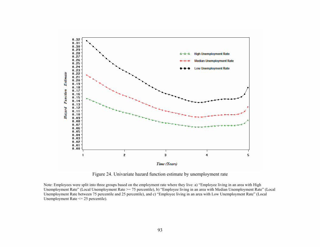
93
Figure 24. Univariate hazard function estimate by unemployment rate
Note: Employees were split into three groups based on the employment rate where they live: a) “Employee living in an area with High Unemployment Rate” (Local Unemployment Rate >= 75 percentile), b) “Employee living in an area with Median Unemployment Rate” (Local Unemployment Rate between 75 percentile and 25 percentile), and c) “Employee living in an area with Low Unemployment Rate” (Local Unemployment Rate <= 25 percentile).

94
The results from the univariate survival model indicated that local
unemployment rates had a significant impact on employees’ employment
duration, although the estimated parameter was not that high -.13 (χ2 (1) =975.61;
p < .0001). The hazard ratio from the univariate model for unemployment rates
and turnover risks was .88, which indicated that one standardized deviation
increase in unemployment rates resulted in a 12% decrease in their turnover risk.
To have a clearer display of the relationship between local unemployment rates
and employees’ turnover risk, employees were split into three groups based on the
employment rate where they live: a) “Employee living in an area with High
Unemployment Rate”, b) “Employee living in an area with Median
Unemployment Rate”, and c) “Employee living in an area with Low
Unemployment Rate”. As demonstrated on Figure 23, approximately 50% of the
employees living in a low-unemployment-rate area would leave the organization
around two and half years. Only 35% of the employees in a median-
unemployment-rate area and 25% of the employees in a high-unemployment-rate
area would quit in the same time. From Figure 24, we could also see similar
results. Employees from areas with high employment rates would face much
higher turnover risks than employees living in areas with low employment rates.
Overall, the hypothesis 6a was supported.
Hypothesis 7a. This hypothesis predicted that local household income
would affect employees’ employment duration. Employees living in an area with
high local household income would be more likely to have longer employment

95
duration than employees from a low-income-area. Following the same procedure,
the averaged local household income across years was used to test hypothesis 7a.
The results from the univariate survival model a weak but statistically
significant association between local household income and employees’
employment duration. The estimated parameter from the univariate survival
model between local economical situation and employees’ turnover risk was -.10
(χ2 (1) =215.06; p < .0001). The hazard ratio was .90, which indicated that one
standardized deviation increase in local household income would result in a 10%
decrease in their turnover risk. Following the same trichotomizing rule,
employees were split into three groups based on the local economical condition
where they live: a) “Employee living in an area with High Household Income”; b)
“Employee living in an area with Median High Household Income”, and c)
“Employee living in an area with Low High Household Income” (see Figure 25
and Figure 26). As demonstrated on Figure 25 and Figure 26, employees living in
high-household-income areas would be more likely to have higher employment
duration and lower turnover risks than ones living in low-household-income
areas, although the differences were not that big. Overall, the hypothesis 8.a was
supported in a moderate way.

96
Figure 25. Univariate survival function estimate by household income
Note: Employees were split into three groups based on the local house hold income where they live: a) “Employee living in an area with High Household Income” (Local Household Income >= 75 percentile), b) “Employee living in an area with Median High Household Income” (Local Household Income between 75 percentile and 25 percentile), and c) “Employee living in an area with Low High Household Income” (Local Household Income <= 25 percentile).
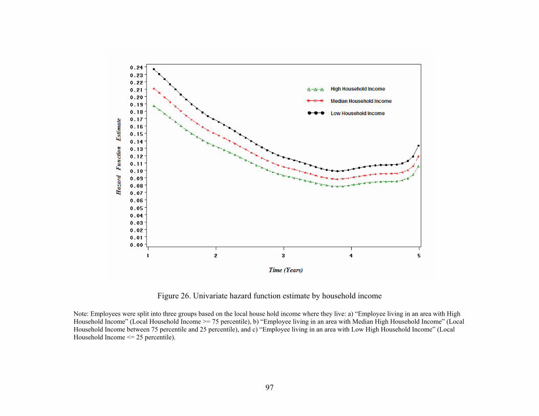
97
Figure 26. Univariate hazard function estimate by household income
Note: Employees were split into three groups based on the local house hold income where they live: a) “Employee living in an area with High Household Income” (Local Household Income >= 75 percentile), b) “Employee living in an area with Median High Household Income” (Local Household Income between 75 percentile and 25 percentile), and c) “Employee living in an area with Low High Household Income” (Local Household Income <= 25 percentile).

98
Latent Growth Modeling (LGM) Analysis Results
As discussed previously, a few predictor variables were conceptually
considered as longitudinal in nature. That is, changes in these variables over time
were believed to be associated with changes in turnover over time. These
longitudinal variables were job performance, compensation, job attitudes, job
satisfaction, intention to quit, local unemployment rate, and local household
income. Latent growth modeling (LGM) was used in the present study to evaluate
if the change patterns for these variables differed for leavers and stayers.
There were three issues related to the LGM analysis that had to be
considered before evaluating the support for my hypotheses. The first issue
centered on sample size limitations of current LGM analysis programs. The
restriction of SAS statistical program limited me to 10,000 participants for this
analysis. Thus, I randomly selected 10,000 participants for my LGM analyses. It
should be noted that I repeated random sampling five times and repeated the
LGM analyses for each random sample. My results were similar across these
different random samples.
The second issue was still related to the actual individuals who had been
included in the LGM analyses. When I conducted survival analyses, only the
employees who had been hired during the six-year study period were included in
the analyses. It was due to the restriction of the requirement of survival model.
However, there was no such restriction of LGM analyses. To take the best use of
the existing data, I included all the employees (employees who were hired before
the study period and those who were hired during the study period). To be parallel

99
with the survival analysis, I also conducted LGM analyses based on the new hire
sample. The results from the new hire sample were very close to the full sample.
Thus, the LGM results reported below were based on the full sample.
The second issue concerned the multi-level results provided by LGM
analysis. The present study focused on whether there were differences between
stayers and leavers on the trend line of the longitudinal variables over time. This
question is only answered by the Level 2 tests provided by LGM analysis. Thus, I
only present Level 2 results in this dissertation (see Table 6).
The first four columns of Table 6 show the LGM Level 2 results for the
intercept. The column labeled γ00 indicates whether there were intra-individual
differences for the longitudinal variable under investigation at the initial time
point of the study - Year 1. The column labeled γ01 indicates the mean value
differences between stayers and leavers on each longitudinal variable at the initial
time point of the study. In other words, this column provides evidence for
whether stayers were initially different from leavers for each longitudinal
variable. For example, the significant value for the γ01 (leavers) on annual pay
rate referred that leavers had different levels of compensation than stayers did at
organizational entry.
The results shown on Table 6 suggested that leavers had significantly
lower compensation levels and lower general attitudes toward the organization
than stayers did at time of entering the organization. Leavers also had
significantly higher levels of intention to quit than stayers at the first year of
employment. It was also found that the Year 1 local unemployment rate for

100
leavers was significantly lower than the Year 1 local unemployment rate for
stayers.
On Table 6, the second four columns demonstrated whether the slope of
each variable was changed with time. The column labeled γ10 provides
information about the rate of change in each variable. The column labeled γ11
answered the question on whether stayers and leavers differed on the slopes of
those predicting variables. The values on Table 6 for γ10 indicated that there was
significant change over time on all the longitudinal variables except for
employees’ performance ratings. That is, compensation levels, job attitudes, and
even local economical conditions were found to change over time. However,
employees’ performance ratings were found to be stable across the six-year study
period. The γ11 column indicates whether stayers and leavers had different
trajectories. It was found that leavers and stayers differed in terms of their rate of
change in compensation, their attitudes towards the organization, and their
intention to quit.
Hypothesis 2b. Hypothesis 2b proposed that employees who turned over
and those who stayed with the organization would have different growth
trajectories in their performance ratings over time. Specifically, it predicted that
the slope of performance ratings for stayers would be more positive than those for
leavers. As shown in Table 6, this hypothesis was not supported by the LGM
results.
The estimated parameters on the initial status of employees’ performance
ratings (γ00 = 2.32, p < .0001; γ01 = 0.04, p = n.s.) indicated that employees did

101
significantly differ in terms of their Year 1 performance ratings, but leavers and
stayers did not significantly differ in terms of Year 1 performance. The LGM
results showed that there were no significant changes in performance ratings over
time and that stayers and leavers did not differ in terms of their change in
performance ratings (γ10 = 0.00, p = n.s.; γ11 = 0.04, p = n.s.) across this study’s
six-year study period. The performance trajectories for stayers and leavers are
plotted on Figure 27. Overall, hypothesis 2b was not supported by the LGM
results.

102
Table 6. Parameter Estimates for Univariate Latent Growth Models
Initial Status Slopes Model Fit Statistics Variables γ00
(Intercept) γ01
(leavers) γ10
(time) γ11
(time*leavers) Deviance AIC BIC
Performance Rating 2.32*** -0.04*** 0.00*** -0.01*** 20,170.5 20,186.5 20,233.5 Annual Pay Rate 0.03*** -0.17*** 0.04*** -0.03*** 3,792.0 3,776.0 3,729.0 Employee Attitudes -0.82*** -0.15*** 0.46*** -0.10*** 25,152.6 25,166.6 25,205.5 Job Satisfaction -0.19*** -0.05*** 0.04*** -0.01*** 16,879.4 16,895.4 16,942.4 Intention to Quit -0.81*** 0.20*** 0.51*** 0.18*** 28,062.9 28,076.9 28,115.8 Local Unemployment Rate 2.93*** -0.38*** 0.41*** -0.02*** 18,142.3 18,158.3 18,198.7
Note. n = 10,000. Except performance rating and local unemployment rate, all other variables were standardized prior to analysis. *** p < .0001; ** p < .001; * p < .01. The results of local household income could not be converged.

103
Figure 27. Latent growth modeling (LGM) graphical results for performance ratings

104
Hypothesis 3b. Hypothesis 3b predicted that employees who left the
organization and those who stayed would have different compensation growth
trajectories; furthermore, the rate of change in pay for stayers would be more
positive than the rate of change in pay for leavers. As shown in Table 6, the
estimated parameters on the initial status of employees’ annual pay rate (γ00 =
0.03, p < .0001; γ01 = 0.17, p = n.s.) indicated that employees differed in terms of
their compensation levels but that stayers and leavers did not significantly differ
in terms of their initial pay levels. The results of the changing trajectories of
employees’ pay rates (γ10 = 0.04, p < .0001; γ11 = -0.03, p < .0001) indicated that
employees’ compensation were changing with time during the six-year study
period and the changing slopes between stayers and leavers were significantly
different. The graphically representation of the results was portrayed in Figure 28.
Overall, hypothesis 3b was supported.
Hypothesis 5.1b. Hypothesis 5.1b predicted that the difference between
stayers and leavers in terms of the changing patterns of their attitudes towards the
organization. It was specifically proposed that stayers would exhibit a more
positive change in their attitudes over time than would leavers. This hypothesis
was strongly supported by the LGM results.
As shown in Table 6, the estimated parameters on the Year 1 difference
among employees’ attitudes towards the organization was quite substantial (γ00 =
0.82, p < .0001) and employees who stayed with

105
Figure 28. Latent growth modeling (LGM) graphical results for annual pay rates

106
the organization reported more initial positive attitudes than those who left (γ01 =
.15, p < .0001). Further, the change in attitudes was significantly different from
zero (γ10 = 0.46, p < .0001). Figure 29 shows these results and reveals that stayers
tended to exhibit a more positive change in attitudes than did leavers. Overall, the
hypothesis 5.1a was supported.
Hypothesis 5.2b. This hypothesis proposed that stayers and leavers would
have different changing trajectories on their job satisfaction. More precisely,
employees who left the organization would exhibit a significantly greater decline
in job satisfaction than would employees who stayed.
The LGM results indicated that employees were significantly differed in
terms of their initial job satisfaction (γ00 = .19, p < .0001), however stayers and
leavers did not differ initially on this variable (γ01 = .05, p = n.s.). Further,
employees’ job satisfaction changed with time (γ10 = .04, p < .0001), but this rate
of change did not significantly differ for stayers and leavers (γ11 = .01, p = n.s.).
Figure 30 demonstrated the trajectories of job satisfaction for leavers and stayers.
From the Figure, we could see that the changing slopes between employees who
quit and those who stayed were similar with each other. Thus, hypothesis 5.2b
was not supported.

107
Figure 29. Latent growth modeling (LGM) graphical results for employees’ attitudes towards the organization

108
Figure 30. Latent growth modeling (LGM) graphical results for overall job satisfaction

109
Hypothesis 5.3b. This hypothesis proposed that employees who stayed
with the organization and those who left would exhibit differences in their
intentions to quit trajectories over time. More specifically, leavers would
increasingly think about quitting.
As shown in Table 6, employees significantly differed in terms of their
initial intention to quit (γ00 = 0.81, p < .0001). Further, employees who stayed
with the organization had much lower initial intentions to quit than those who
turned over (γ01 = .20, p < .0001). In terms of the rate of change in this variable,
employees’ intention to quit was found to significantly change over time (γ10 =
0.51, p < .0001) and, more importantly, the rate of change in this variable
significantly differed between stayers and leavers (γ10 = 0.18, p < .0001). Figure
31 shows this result and it can be seen that leavers level of intention to quit over
time significantly increased over time in comparison to the stayers. Stayers
intention to quit trajectory actually decreased over time. Thus, hypothesis 5.3b
was fully supported by the results.
Hypothesis 6b. This hypothesis proposed that the change of local
unemployment over time would be different between employees who left versus
those who stayed. Specifically, it was predicted that the unemployment rate slope
for stayers would be more positive than the slope for leavers.
The LGM results indicated that employees differed in terms of their initial
local unemployment rates (γ00 = 2.93, p < .0001) and that stayers came from areas
with higher local unemployment-rate areas than did leavers (γ01 = .38, p < .0001),

110
Figure 31. Latent growth modeling (LGM) graphical results for intention to quit

111
Table 6 also shows that the local employment rates changed over time (γ10 = .41,
p < .0001). However, there were no significant differences in the rate of change
of the local employment rate between stayers and leavers (γ11 = .01, p = n.s.).
Thus, hypothesis 6b was not supported by the results.
Additional Post Hoc Investigations
In the previous survival analyses, the univariate relation between each of
the predictor variables and turnover risk was evaluated. The univariate survival
analyses evaluated the univariate association between one predictor and turnover
risk. To compare the relative strengths of the associations between each of the
predictors and turnover, a multivariate survival model was applied. The
multivariate model included all the predictors into the same model, which
evaluated the associations between predictors and dependent variable
simultaneously. The multivariate survival results were presented in Table 7,
which presented the strength of the relationships between each predictor variable
and turnover risk, after controlling the influence of other variables.
The results of the univariate survival model indicated a significant
relationship between each of the predictors and turnover risk. The results of the
multivariate survival model indicated a different story. Employees’ age,
performance ratings, and their local household income were found not having a
significant association with the survival and hazard functions, after controlling the
impact of other variables. Employees’ annual pay rate, their promotion, their
intention to quit, and their job satisfaction were found to have strong impact on
the turnover risk. Additionally, employees’ attitudes toward the organization and

112
Table 7. Multivariate Survival Model Predicting Employment Duration
Parameter Estimate
Standard Error Chi-Square Hazard
Ratio Gender -0.19 0.07 8.17**** 0.79 Age -0.06 0.04 1.92*** 0.94 Performance Rating -0.08 0.05 2.48*** 0.92 Annual Pay Rate -1.42 0.08 290.19*** 0.24 Promotion -0.56 0.05 143.50*** 0.57 Employee Attitudes -0.17 0.06 8.49*** 0.84 Job Satisfaction -0.17 0.04 22.27*** 0.82 Intention to Quit 0.94 0.04 684.63*** 1.61 Local Unemployment Rate -0.10 0.03 11.11** 0.90 Local Household Income -0.09 0.04 9.55*** 0.99
Note. All the continuous predictors were standardized prior to analysis. *** p < .0001; ** p < .001; * p < .01. All the variables were standardized before conducting the survival analyses.
their local unemployment rates were moderately related to employees’ survival
and hazard function. The following section interpreted the results of the
multivariate model in detail.
After controlling other variables, employees’ psychological predictors
were found to have significant association with turnover hazard. For example,
employees’ intentional to quit had the strongest impact on turnover risks. The
estimated parameter for intention to quit was 0.94 (χ2 (10) = 684.63; p < .0001)
and the hazard ratio for this predictor was 1.61. Employees’ job satisfaction was
also found being negatively related with higher hazard function. The estimated
parameter for job satisfaction was -0.17 (χ2 (10) = 22.27, p < .0001) and the
hazard ratio was 0.82. Additionally, employees’ attitudes toward the organization
was significantly negatively related to turnover, with the estimated parameter as -
0.17 (χ2 (10) = 8.49; p < .01) and the hazard ratio as 0.84. That is, in this model,

113
after controlling other variables, a 1-standard-deviation increase in intention to
quit added the turnover hazard by 60% and a 1-standard-deviation increase in job
satisfaction and general attitudes reduced turnover risk by 20%.
The results of the multivariate model also indicated that employees’
human resource management predictors were significantly related to turnover
risks. Employees’ annual pay rate was the second strongest predictor among all
the variables. The estimated parameter for intention to quit was -1.42 (χ2 (10) =
290.19; p < .0001) and the hazard ratio for this predictor was 0.24. Promotion was
also found to be associated with turnover hazard, with the estimated parameter as
-0.56 (χ2 (10) = 143.50; p < .0001) and the hazard ratio as 0.54. That is, a one-
standard-deviation increase in employees’ annual pay rate reduced turnover risk
by 75% and one time increase in promotion decreased turnover hazard by 40%.
However, the performance rating was shown to have no significant relationship
between turnover risks when other variables were also in the survival model.
The results of the multivariate survival model show that employees’
individual demographical predictors had weak associations with turnover hazard.
Gender was found to be moderately related to turnover risks. The estimated
parameter for gender was -0.19 (χ2 (10) = 8.17; p < .01) and the hazard ratio was
0.79. It indicated that females had 20% higher turnover risk than males. However,
age was found having no significant relation with turnover hazard, with the
estimated parameter as -0.06 (χ2 (10) = 1.92; p = n.s.) and the hazard ratio as 0.94.
Finally, external economical factors were also found to be moderately
related to turnover risks. The local unemployment rate had a weak but significant
114
association with the hazard function. The estimated parameter was -0.10 (χ2 (10)
= 11.11; p < .001) and the hazard ratio was 0.90). However, the local household
income was not related to turnover risks, with estimated parameter as -0.09 (χ2
(10) = 9.55; p = n.s.)
Univariate Model versus Multivariate Model
The results based on the univariate survival model and the multivariate
survival model told us a similar but not exactly same story (see Table 8). No
matter with controlling influences from other predictors or without controlling,
annual pay rate (effect size = -0.62 & -0.76), promotion (effect size = -0.56 & -
0.43), and intention to quit (effect size = +0.77 & +0.61) were indicated to be
strongly associated with turnover behaviors over time. Gender (effect size = -0.10
& -0.21), local unemployment rate (Effect size = -0.12 & -0.10) and local
household income (effect size = -0.10 & -0.01) were shown to be weakly related
to turnover risks over time. Thus, the previous predictors held a robust
relationship with turnover hazard over time with or without controlling other
factors. However, age and performance rating were found to be strongly related to
turnover risks when other factors were not controlled, while these relationships
became weak when the influence from other predictors were controlled. For
instance, based on the univariate model, hazard ratio for age was 0.12 (effect size
= -0.88), indicating a strong association between age and turnover risks. But,
based on the multivariate model, hazard ratio for age was 0.94 (effect size = -
0.06), indicating a weak relationship. The results for performance rating also

115
indicated that the strength of the association between performance and turnover
risks became weak when other influences were taken out.
Overall, the comparison between the results based on the univariate
survival model and the multivariate survival model provided more evidences
about the time effect of turnover process. It indicated that the relationship
between predictors and turnover risks changed over time. No matter controlling or
not controlling other predictors, actual management factors and psychological
indicators were found to be strongly association with turnover hazards. The
association between turnover risks and demographical indicators or external
economical factors became moderate or weak after controlling the influence from
other predictors.
Table 8. Univariate Survival Model versus Multivariate Survival Model
Univariate Survival Model Multivariate Survival Model Hazard Ratio Effect Size Hazard Ratio Effect Size Gender 0.90 -0.10 0.79 -0.21 Age 0.12 -0.88 0.94 -0.06 Performance Rating 0.71 -0.29 0.92 -0.08 Annual Pay Rate 0.38 -0.62 0.24 -0.76 Promotion 0.44 -0.56 0.57 -0.43 Employee Attitudes 0.35 -0.65 0.84 -0.16 Job Satisfaction 0.47 -0.53 0.82 -0.18 Intention to Quit 1.77 +0.77 1.61 +0.61 Local Unemployment Rate 0.88 -0.12 0.90 -0.10 Local Household Income 0.90 -0.10 0.99 -0.01
Note. The effect size is represented by the percentage change of turnover along with one unit change of predictors.

116
DISCUSSION
The importance of time and change in the prediction of turnover risks was
demonstrated by the present study. By investigating how employees’ turnover
behaviors could be predicted by predictors and by the changing trajectories of
those predictors over time, the current study enabled researchers to have a better
understanding of several questions related to turnover studies, while providing
suggestions for future research on this topic. The results of survival analyses
indicate that psychological indicators, including employees’ general attitudes
towards the organization, their job satisfaction, and their intention to quit, have
strong association with turnover risks over time. Management predictors, such as
employees’ compensation levels and their promotion history also have strong
relations with turnover hazards over time. And, the results of growth modeling
show that not only predictors’ initial levels but also their changing patterns have
strong relationships with turnover risks. Overall, survival analyses and growth
modeling analyses provide an opportunity for researchers to have a better
understanding of the relations between predictors and turnover longitudinally.
Contribution
As discussed previously, this study explored the prediction of turnover
functions over time, using predictors from diverse resources. The present study
contributes to turnover research in several ways. First, by applying the survival
analysis and the LGM analysis to a six-year longitudinal data set, the present
study investigated the time and change effect of predictors on turnover risks,
which had been neglected by many previous turnover studies. Specifically, the

117
results of the survival analyses demonstrated the time effect on turnover risks. For
example, from the survival function and the hazard figures, researchers could find
out what was the specific turnover risk for certain employees at certain point of
time. For the employees in the present study, their turnover risks were changing
over time. They were facing the highest turnover hazard during their first year of
employment. Additionally, the LGM analysis provided an opportunity to evaluate
the relationship between the dynamic predictors and turnover risks, by several
estimated parameters of the LGM analysis, such as γ00, γ01, γ10, and γ11. In the
present study, all the assumed dynamic predictors, expect employees’
performance rating, were found to be changing with time. The dynamic patterns
of employees’ annual pay rate, their attitudes towards the organization, and their
intention to quit were significantly related with turnover behaviors.
The second contribution of the present study was to compare the strength
of predicting powers among predictor variables from different sources, including
self-reported psychological predictors, actual management indicators, employees’
demographics, and the external economical factors. Previous turnover research
primarily used self-reported survey data for attitude to behavior turnover
predictors. The current study included data from other sources besides survey
data, such as actual management predictors and external economical factors into
same analyses. Although a few meta-analyses (Home and Griffeth, 1995) had
compared the strength of predicting power between psychological or attitudes
indicators and actual event or behavior predictors, those comparison was not
conducted on the exactly same samples. The present study allowed researchers to

118
have a more accurate evaluation of the predicting strength from different
predictors on the same sample.
Because of the second contribution, the present study allowed researchers
to examine the importance of the psychological predictors in terms of their
associations with turnover risks. As addressed previously, the results of the
survival analyses and the LGM analyses revealed the powerful role of
psychological predictors in predicting turnover risks. Indeed, based on the
univariate survival model, employee attitudes toward the organization, their
intention to quit, and their job satisfaction were all significantly associated with
the survival and hazard function over time (p <.0001). Even after controlling the
influence from other predictors, such as demographics, management predictors,
and external economical factors, those three psychological indictors were still
shown to have significant relation with turnover risks. Intention to quit was the
strongest predictor among all variables, with one of the highest hazard ratios (p
<.0001). Employees’ attitudes about the organization and their job satisfaction
were also significantly related to turnover hazard. The LGM analyses also
indicated that, except job satisfaction, the other two psychological predictors had
an impact on employees’ turnover risks.
Furthermore, the present study also allowed researchers to assess the
influence of employees’ actual compensation and actual promotion on the
turnover hazard. Previous turnover studies on compensation had primarily
focused on whether dissatisfaction with salary and pay strongly underlie turnover
(Gomes-Meija & Balkin, 1992; Milkovich & Newman, 1993). Not many studies
119
had evaluated whether actual compensation would be related to turnover. This
could be the reason for very littler direct support on the relationship between
compensation and turnover. The current research indicated that employees’ actual
compensation was one the strongest predictors among all the variables. Indeed, no
matter based on the univariate or the multivariate survival model, employees’
annual pay rate was significantly associated with their survival and hazard
function over time (p <.0001). The LGM analyses also indicated that the changing
patterns of employment compensation were different for leavers and stayers.
Previous meta-analyses on promotion and turnover risks had shown that, although
satisfaction about promotion and perceived opportunities for promotion
moderately predicted turnover, actual promotion strongly predicted turnover
(Hom & Griffeth, 1995). The current study supported the previous results. For
both univariate and multivariate survival analyses, the actual promotion was
proved to be significantly related to turnover.
Additionally, the present study also allowed researchers to assess the
impact of employees’ demographics and the external economical situations on the
turnover decisions. Previous studies had shown that those predictors were
significantly related to turnover risks. The results of the univariate survival model
supported this view. However, the multivariate survival analyses indicated that,
after controlling the influence of other predictors, demographics and economical
factors had no relations or moderate relations with turnover risks. Indeed, gender
and local unemployment rate were found to be moderately associated with
turnover hazards (p <.01 and p <.001, respectively). Age and local household

120
income were not found to be related to turnover risks after controlling influences
from other predictors.
The results of the present study also contribute to the understanding of the
dynamic nature of turnover predictors. As discussed previously, the LGM
provided researchers an opportunity to evaluate whether a variable was changing
with time. The estimated parameter - γ10 – was used to examine whether the
studying variable was predicted by time. In the hypothesis section, it had been
proposed that several predictors were dynamic and they were changing over time.
For example, employees’ job performance, their annual pay rate, and their
attitudes were proposed to fluctuate over time. The results revealed that
employees’ compensation and attitudes increase or decrease with time. However,
employees’ job performance was found to be stable over time.
Future directions and Limitations
By including predictors from multiple sources, this longitudinal study
helped to stimulate future research in several research directions. First, our
findings suggested the need for more empirical examinations of the dynamic
nature of predictors. For example, the assumption that performance was stable
had been debated for many years. From the early theoretical work to the current
empirical studies, it had been indicated that the stability assumption of job
performance was false and performance was changing over time (Deadrick,
Bennett, & Russell, 1997; Ghiselli (1956); Hanges, Schneider, & Niles, 1990;
Hofmann, Jacobs, & Gerras, 1992; Ployhart & Hakel, 1998; Wernimont and
Campbell (1968). However, in this study, job performance was found to be stable

121
over time. That is, for most of the employees, their performance ratings kept in
the same level during the six-year study period. The results of this study seemed
conflict with the previous instability assumption of performance. However, it had
to notice an important issues related to performance ratings in this study before
making the conclusion. There were three categories of the performance ratings: a)
Exceeds expectations, b) Meets expectations, and c) Needs improvements. Figure
32 demonstrated the percentages of each category over six years. This figure
indicated that, in every year, over 70% of the employees having their performance
ratings as “Meets expectations”. About 25% of the employees were rated as
“Exceeds expectations”. And, only 5% employees were categorized as “Needs
improvement”. The percentages of these three types of ratings were stable across
years. One of the reasons leading a stable performance could be the limitation of
the three categories. Because these categories did not have enough distinguish
power to rate employees’ performance, there were no enough variances in
performance to reveal its’ instability nature. Thus, future study on performance
and turnover could continue on the dynamic nature of performance as a turnover
antecedent. Specifically, more accurate performance rating scale should be
applied to have a better understanding of the dynamic nature of performance and
turnover risks.
Another area for future research was to understand the turnover hazard of
employees whose employment duration was higher than six years. In the present
study, due to the restriction of the six-year study period, the relations between
predictors and turnover were only evaluated during six years. Previous meta-

122
Figure 32. Performance Ratings Splitting by Categories
analyses had shown that employees’ tenure was related to their turnover behaviors
(Hom & Griffeth, 1995). That is, the longer employees’ employment duration
was, the lower turnover risk employees would have. Thus, turnover hazards
would be influenced by time. However, this study only examined the relations
between predictors and turnover risks within six years. What would the relation
be if employees had longer employment duration? This study left the question
unsolved. I conducted the survival analyses on all the employees, including the
employees who hired during the six-year study period and those who hired before
the beginning of the study period. These analyses allowed to evaluate the
relationship between the predictors and employment duration for a greater range
(time > 6 years).

123
It should be noted, however, that the hazard functions based on all the
employees in the present study were biased, because it did not include employees
who left the organization before the study period. Thus, the results of survival
analyses were weighted more on the employees who had already been in the
organization for over six years. The results of the univariate and multivariate
survival analyses based on all the employees were presented on table 8. The
results based on all the employees were telling a similar story with the previous
results. Besides that, the results provided information about the survival and
hazard function beyond the six-year study period.
Table 8. Univariate and Multivariate Survival Model Predicting Employment Duration (with all the employees)
Univariate Survival Model Multivariate Survival Model Chi-Square Hazard Ratio Chi-Square Hazard Ratio
Gender 55.38*** 0.90 8.17*** 0.79 Age 5958.21*** 0.12 1.92*** 0.94 Performance Rating 568.11*** 0.71 2.48*** 0.92 Annual Pay Rate 3237.42*** 0.38 290.19*** 0.24 Promotion 3101.23*** 0.45 143.50*** 0.57 Job Attitudes 9523.21*** 0.35 8.49*** 0.84 Job Satisfaction 457.21*** 1.53 22.27*** 1.18 Intention to Quit 7277.71*** 0.23 684.62*** 0.39 Local Unemployment Rate 251.56*** 0.91 11.11*** 1.10 Local Household Income 194.56*** 0.95 9.05*** 1.01
Note. All the continuous predictors were standardized prior to analysis. *** p < .0001. Full sample included all the employees in the organization (n = 95,859).
For example, the estimated survival and hazard functions by employees’
attitudes towards their organization were demonstrated by Figure 33 and Figure
34. According to Figure 33, it could be seen that, during the first five-year
employment, about 55% of the employees with negative attitudes, about 20% of

124
the employees with neutral attitudes, and about 5% of the employees with positive
attitudes, would leave the organization. The changing patterns of the hazard
function for employees with different attitudes were different, too. During the
thirty years employment period, employees with negative attitudes always had
higher hazard risks than other employees. Their turnover hazards varied the most.
Those employees were facing the highest risk to quit during the first ten years and
the last ten years.
Two final caveats must be considered regarding the results of this study.
First, the psychological predictors and the attitude indicators were collected once
a year. That is, one wave of data was used to present employees’ psychological
conditions across the whole year. Thus, no matter when the employees left the
organization during the year, those turnover behaviors were predicted by the one
set of data collected in the summer. The interval between the time to collect
psychological variables and the time of actual turnover behaviors ranged from one
month to twelve months. This could affect the relation between those predictors
and turnover risks. For example, the relationship between employees’ job
satisfaction and turnover risks with three-month interval might be different from
the relationship between those two variables with twelve-month interval. To have
a better understanding of the relationship between psychological predictors and
turnover hazards over time, monthly collected data would be better than the
yearly one. Thus, future studies focusing on the interval of the data collections of

125
Figure 33. Survival function estimate by employee attitudes towards the organization (with all employees)
Note: Employees were split into three groups according to their attitudes: a) “Positive Attitudes” (Attitudes scores >= 75 percentile), b) “Neutral Attitudes” (Attitudes score between 75 percentile and 25 percentile), and c) “Negative Attitudes” (Attitudes score <= 25 percentile).

126
Figure 34. Hazard function estimate by employee attitudes towards the organization (with all employees)
Note: Employees were split into three groups according to their attitudes: a) “Employee with Positive Attitudes” (Attitudes scores >= 75 percentile), b) “Employee with Neutral Attitudes” (Attitudes score between 75 percentile and 25 percentile), and c) “Employee with negative Attitudes” (Attitudes score <= 25 percentile).

127
predictors and actual outcomes would be benefit our understanding of the
dynamic process of turnover.
Second, although the study involved a much more diverse sample than
many turnover studies, which varied from higher level top managers to the lower
job level contractors. Also, the job families included administrative supportive,
business operations, clinical and pharmaceutical, customer service and claims,
healthcare operations, sales and marketing, and technology. But, all the
participants were from one organization. Their average salary was higher than the
average pay across the whole population. Thus, they might have a different
process of turnover because of the nature of this specific organization. Future
research exploring the generalizability of these results to people working for other
type of companies could provide a more accurate illustration of the relations
between those predictors and turnover.

128
Appendix A. Employee Attitudes Survey
Instructions
The annual Employee Attitudes Survey will provide the company leaders with valuable information on what the organization does well and where improvements are needed in delivering services to its customers, as well as making it a better place to work. Your responses to this questionnaire are completely anonymous. Please place your completed questionnaire in the enclosed postage-paid return envelope, and then place it in any mailbox. Please read each question carefully and pick the answer that best describes your opinion. Pick only one answer and shade the appropriate circle to indicate your response. If a question does not apply to you, or you don’t know how to answer, skip the question or fill in the choice labeled “6 – Don’t know / Not Applicable”. To what extent do you agree or disagree with each of the following statements about the COMPANY? Indicate one answer for each statement.
1 2 3 4 5 6
Strongly Agree Agree
Neither Agree nor Disagree
Disagree Strongly Disagree
Don’t Know/Not Applicable
This Company has a clear sense of direction. (1) (2) (3) (4) (5) (6)
All in all, the changes we are making will make us a better Company. (1) (2) (3) (4) (5) (6)
This Company’s senior management’s actions are consistent with their words. (1) (2) (3) (4) (5) (6)
My job makes good use of my skills and abilities. (1) (2) (3) (4) (5) (6)
I have a clear idea of the results expected of me in my job. (1) (2) (3) (4) (5) (6)
This Company's senior management demonstrates that employees are important to the success of the business. (1) (2) (3) (4) (5) (6)
This company's senior management demonstrates that employees are important to the success of the business. (1) (2) (3) (4) (5) (6)
Overall, this Company is an effectively managed, well-run business. (1) (2) (3) (4) (5) (6)
I feel proud to work for this Company. (1) (2) (3) (4) (5) (6)
This company is a great place to work, compared to other organizations I know about. (1) (2) (3) (4) (5) (6)
I am enthusiastic about my future with this Company as a place to work and develop my skills. (1) (2) (3) (4) (5) (6)
My work gives me a feeling of personal accomplishment. (1) (2) (3) (4) (5) (6)

129
Considering everything, how would you rate your overall satisfaction in the Company at the present time? Indicate ONE answer:
(1) Very Satisfied (2) Satisfied (3) Neither satisfied nor dissatisfied (4) Dissatisfied (5) Very dissatisfied
How long do you expect to continue working for this Company? Indicate ONE answer:
(1) Less than 1 year (2) 1-3 years (3) More than 3 years to less than 5 years (4) More than 5 years to less than 10 years (5) 10 years or more (6) Until retirement

130
Appendix C. SAS Program Used for CFA of the Employee Attitudes Measurement
data AttitudeSurvey(TYPE=CORR); _type_ = 'corr'; input _name_ $ V1 V2 V3 V4 V5 V6 V7 V8 V9 V10 V11 V12 V13 V14 V15; datalines; V1 1.000 V2 0.473 1.000 V3 0.500 0.468 1.000 V4 0.275 0.298 0.233 1.000 V5 0.284 0.268 0.203 0.471 1.000 V6 0.446 0.517 0.397 0.350 0.313 1.000 V7 0.493 0.477 0.577 0.286 0.262 0.558 1.000 V8 0.589 0.463 0.601 0.283 0.247 0.428 0.535 1.000 V9 0.519 0.476 0.448 0.382 0.328 0.514 0.555 0.561 1.000 V10 0.465 0.426 0.381 0.348 0.295 0.524 0.469 0.467 0.588 1.000 V11 0.418 0.569 0.357 0.466 0.372 0.584 0.487 0.410 0.614 0.526 1.000 V12 0.306 0.338 0.252 0.754 0.512 0.393 0.323 0.304 0.460 0.399 0.530 1.000 ; RUN; proc calis data=UHG2004 method=max edf=25000 pestim se; Lineqs V1 = X1 F1 + E1, V2 = X2 F1 + E2, V3 = X3 F1 + E3, V4 = X4 F2 + E4, V5 = X5 F2 + E5, V6 = X6 F3 + E6, V7 = X7 F3 + E7, V8 = X8 F4 + E8, V9 = X9 F4 + E9, V10 = X10 F4 + E10, V11 = X11 F4 + E11, V12 = X12 F4 + E12, F1 = X13 F5 + E13, F2 = X14 F5 + E14, F3 = X15 F5 + E15, F4 = X16 F5 + E16; Std F5 = 1. , E1-E12 = U11-U112 , E13-E16 = 4 * 1.; Bounds 0. <= U11-U112;
run;

131
Appendix C. SAS Example Program Used for Survival Analyses
*Univariate Survival Analysis; *H1a: Female employees will be less likely to quit than male employees; Proc PHREG data = Full_Data; Model Employment_Duration * Turnover_Voluntary(0) = Gender; Run; *Graphic Descriptions – Survival Curves; Data IN00; Input Gender; Cards; 1 2 ; PROC PHREG Data = Full_Data noprint; Model Employment_Duration * Turnover_Voluntary(0) = Gender; Baseline Covariates = IN00 Out = Gender Survival = S1/Nomean; Run; Proc GPLOT Data = Gender; PLOT S1 * Employment_Duration = gender; symbol1 i= SM c=blue v= dot height=.5; symbol2 i= SM c=red v= star height=.5; Run; *Multivariate Survival Analysis; Proc PHREG data = Full_Data; Model Employment_Duration * Turnover_Voluntary(0) = Gender Age Performance Pay Promotion Attitudes JSAT ITQ Unemployment Income; Baseline Out = overall Survival = S1/Nomean; Run;

132
Appendix D. SAS Example Program Used for Growth Modeling Analyses *H2b: Leavers and stayers will have different growth trajectories in their performance over time; Proc mixed data = Full_Data method = ml covtest; class EEID; model Performance = Time Turnover Time*Turnover/ solution; random intercept Time / type = un subject = EEID ; run;

133
References
Allen, N.J., & Meyer, J.P. (1990). The measurement and antecedents of
affective, continuance and normative commitment to the organization. Journal of
Occupational Psychology, 63, 1-18.
Ancona, D.G., Goodman, P.S., Lawrence, B.S., & Tushman, M.L. (2001).
Time: A new research lens. Academy of Management Review, 26, 645-663.
Barrett, G.V., Caldwell, M.S., & Alexander, R.A. (1985). The concept of
dynamic criteria: A critical reanalysis. Personnel Psychology, 38, 41-57.
Becker, B.E., Huselid, M.A., & Ulrich, D. (2001). The human resources
scorecard: Linking people, strategy, and performance. Boston: Harvard Business
School Press.
Bentein, K., Vandenberg, R., Vandenberghe, C., & Stinglhamber, F.
(2005). The role of change in the relationship between commitment and turnover:
A latent growth modeling approach. Journal of Applied Psychology, 90, 468-482.
Blau, G., & Boal, K. (1987). Conceptualizing how job involvement and
organizational commitment affect turnover and absenteeism. Academy of
Management Review, 12, 288-300.
Blau, G. J., & Boal, K. B. (1989). Using job involvement and
organizational commitment interactively to predict turnover. Journal of
Management, 15, 115-127.
Bluedorn, A.C., & Denhart, R.B. (1988). Time and organizations. Journal
of Management, 14, 299-320.

134
Brockner, J., Tyler, T.R., & Cooper-Schneider, R. (1992). The effects of
prior commitment to an institution on reactions to perceived unfairness: The
higher they are, the harder they fall. Administrative Science Quarterly, 37, 241-
261.
Bryk, A.S., & Raudenbush, S.W. (1987). Application of hierarchical linear
models to assessing change. Psychological Bulletin, 101, 147-158.
Burstein, L. (1980). The analysis of multilevel data in educational research
and evaluation. Review of Research in Education, 8, 158-233.
Bycio, P., Hackett, R.D., & Alvares, K.M. (1990). Job performance and
turnover: A review and meta-analysis. Applied Psychology: An International
Review, 39, 47-76.
Carsten, J.M., & Spector, P.E. (1987). Unemployment, job satisfaction,
and employee turnover: A meta-analytic test of the Muchinsky model. Journal of
Applied Psychology, 72, 374-381.
Chan, D. (1998). The conceptualization and analysis of change over time:
An integrative approach incorporating longitudinal mean and covariance
structures analysis (LMACS) and multiple indicator latent growth modeling
(MLGM). Organizational Research Methods, 1, 421-483.
Chan, D., & Schmitt, N. (2000). Interindividual differences in
intraindividual changes in proactivity during organizational entry: A latent growth
modeling approach to newcomer adaptation. Journal of Applied Psychology, 85, 190-
210.

135
Clark, P. (1985). A review of the theories of time and structure for
organizational sociology. In S.B. Bacharach and S.M. Mitchell (eds.), Research in
the Sociology of Organizations. Greebwich, CT: JAI Press.
Cotton, J.L., & Turtle, J.M. (1986). Employee turnover: A meta-analysis
and review with implications for research. Academy of Management Review, 11,
55-70.
Cox, D.R., & Oakes, D. (1984). Analysis of survival data. Chapman &
Hall / CRC Press.
Cox, D.R. (1972). Regression models and life-tables (with discussion).
Journal of the Royal Statistical Society, Series B, 34, 187-220.
Day, N. E. (1987). Clarifying the relationship between organizational
commitment and performance. Unpublished doctoral dissertation, University of
Kansas.
Deadrick, D.L., Bennett, N., & Russell, C.T. (1997). Using hierarchical
linear modeling to examine dynamic performance criteria over time. Journal of
Management, 23, 745-754.
Deadrick, D.L., & Madigan, R.M. (1990). Dynamic criteria revisited: A
longitudinal study of performance stability and predictive validity. Personnel
Psychology, 43, 717-744.
Delery, J.E., & Shaw, J.D. (2001). The strategic management of people in
work organizations: Review, synthesis and extension. In. K.M. Rowland & G.R.
Ferris (eds.), Research in Personnel and Human Resource Management.
Greenwich, CT: JAI Press.

136
Dickter, D.N., Roznowski, M., & Harrison, D.A. (1996). Temporal
tempering: An event history analysis of the process of voluntary turnover. Journal
of Applied Psychology, 81, 705-716.
Duncan, T.E., Duncan, S.C., Strycker, L.A., Li, F., & Alpert, A. (1999).
An introduction to latent curve modeling: Concepts, issues, and applications.
Mahwah, NJ.: Lawrence Erlbaum Associates, Inc.
Fombrun, C. (1996). Reputation. Boston: Harvard Business School Press.
Gardner, W., & Griffin, W.A. (1989). Methods for the analysis of parallel
streams of continuously recorded social behaviors. Psychological Bulletin, 105,
446-455.
Gerhart, B. (1987). How important are dispositional factors as
determinants of job satisfaction? Implications for job design and other personnel
programs. Journal of Applied Psychology, 72, 366-373.
Gerstner, C.R., & Day, D.V. (1997). Meta-analytic review of Leader-
Member Exchange theory: Correlates and construct issues. Journal of Applied
Psychology, 82, 827-844.
Gomez-Mejia, L.R., & Balkin, D.B. (1987). The determinants of
managerial satisfaction with the expatriation and repatriation process. Journal of
Management Development, 6, 7-17.
Greenhouse, J.B., Stangl, D., & Bromberg, J. (1989). An introduction to
survival analysis: Statistical methods for analysis of clinical trial data. Journal of
Consulting and Clinical Psychology, 57, 536-544.

137
Griffeth, R. W., Hom, P. W., & Gaertner, S. (2000). A meta-analysis of
antecedents and correlates of employee turnover: Update, moderator tests, and
research implications for the next millennium. Journal of Management, 26.
Gurvitch, G. (1964). The problem of time. In J. Hassard (ed.), The
sociology of time. London: Macmillan.
Hanges, P.J., Lord, R.G., Godfrey, E.G., & Raver, J.L. (2002). Modeling
nonlinear relationships: Neural networks and catastrophe analysis. In S.
Rogelberg (ed.), Handbook of research methods in industrial and organizational
psychology. Malden, MA: Blackwell Publishers, Inc.
Hanges, P.J., Schneider, B., & Niles, K. (1990). Stability of performance:
An Interactionist Perspective. Journal of Applied Psychology, 75, 658-667.
Harrison, D.A., & Hulin, C.L. (1989). Investigations of absenteeism:
Using event history models to study the absence-taking process. Journal of
Applied Psychology, 74, 300-316.
Harrison, D.A., Virick, M., & William, S. (1996). Working without a net:
Time, performance, and turnover under maximally contingent rewards. Journal of
Applied Psychology, 81, 331-345.
Heneman, H.G. (1985). Pay satisfaction. In K.M. Rowland and G.R. Ferris
(eds.), Research in personnel and human resources management. Greenwich,
Conn.: JAI Press.
Henry, R.A., & Hulin, C.L. (1987). Stability of skilled performance across
time: Some generalizations and limitations on utilities. Journal of Applied
Psychology, 72, 457-462.

138
Hofmann, D.A., Jacobs, R., & Baratta, J.E. (1993). Dynamic criteria and
the measurement of change. Journal of Applied Psychology, 78, 194-204.
Hofmann, D.A., Jacobs, R. & Gerras, S.J. (1992). Mapping individual
performance over time. Journal of Applied Psychology, 77, 185-195.
Hom, P. (1992). Turnover costs among mental health professionals.
College of Business, Arizona State University, Tempe, Ariz.
Hom, P., Caranikis-Walker, F., Prussia, G., & Griffeth, R. (1992). A meta-
analytical structural equations analysis of a model of employee turnover. Journal
of Applied Psychology, 77, 890-909.
Hom, P., & Griffeth, R. (1995). Employee turnover. Cincinnati, OH:
Southwestern.
Hom, P., Griffeth, R., Palich, L., & Bracker, J.S. (1993). Realistic job
previews: Two-occupation test of mediating processes. College of Business,
Arizona State University, Tempe, Ariz.
Hom, P.W., & Kinicki, A.J. (2001). Toward a greater understanding of
how dissatisfaction drives employee turnover. Academy of Management Journal,
44, 975-87.
Hulin, C.L. (1991). Adaptation, persistence, and commitment in
organizations. In D. Dunnette and L. Hough (eds.), Handbook of industrial and
organizational psychology, 2, 445-506. Palo Alto, CA: Consulting Psychologists
Press.

139
Hulin, C.L., Roznowski, M., & Hachiya, D. (1985). Alternative
opportunities and withdrawal decisions: Empirical and theoretical discrepancies
and an integration. Psychological Bulletin, 97, 233-250.
Huselid, M.A. (1995). The impact of human resource management
practices on turnover: Productivity, and corporate financial performance.
Academy of Management Journal, 38, 635-672.
Jovanovic, B. (1979). Firm-specific capital and turnover. Journal of
Political Economy, 87, 1246-1261.
Kammeyer-Mueller, J.D., Wanberg, C.R., Glomb, T.M., & Ahlburg, D.
(2005). The Role of Temporal Shifts in Turnover Processes: It's About Time.
Journal of Applied Psychology, 90, 644-658.
Katz, D., & Kahn, R.L. (1978). The social psychology of organizations.
New York: Wiley Press.
Lance, C.E., Meade, A.W., & Williamson, G.M. (2000). We should
measure change – And here’s how. In G.M. Williamson and D.R. Shaffer (eds.),
Physical illness and depression in older adults: A handbook of theory, research
and practice, pp. 201-235. New York: Plenum.
Lee, T.W., & Mitchell, T.R. (1994). An alternative approach: The
unfolding model of voluntary employee turnover. Academy of Management
Review, 19, 51-89.
Levinthal, D.A., & Fichman, M. (1988). Dynamics of interorganizational
attachments: Auditor-Client relationships. Administrative Science Quarterly, 33,
345-369.
140
Mandel, M.J., & Farrell, C. (1992, July 13). The immigrants. Business
Week, 114.
March, J.G., & Simon, H.A. (1958). Organizations. New York: Wiley.
Mason, W.M., Wong, G.M., & Entwistle, B. (1983). Contextual analysis
through the multilevel linear model. In S. Leinhardt (ed.), Sociological
methodology. San Francisco: Jossey-Bass.
Maslach, C., Schaufeli, W.B., & Leiter, M.P. (2001). Job burnout. Annual
Review of Psychology,52, 397–422.
Marion, R. (1999). The edge of organization: Chaos and complexity
theories of formal social organization. Newbury Park, CA: Sage.
McEvoy, G.M., & Cascio, W.F. (1987). Do good or poor performers
leave? A meta-analysis of the relationship between performance and turnover.
Academy of Management Journal, 30, 744-762.
Meyer, J.P., & Allen, N.J. (1997). Commitment in the workplace: Theory,
research, and application. Sage Publications Inc.
Milkovich, G.T., & Newman, J.M. (1993). Compensation (4th ed.).
Homewood, IL: Irwin.
Miller, R.G., JR. (1981). Simultaneous statistical inference. McGraw Hill,
NY.
Mitchell, T.R., & James, L.R. (2001). Building better theory: Time and the
specification of when things happen. Academy of Management Review, 26, 530-
547.

141
Mobley, W.H. (1977). Intermediate linkages in the relationship between
job satisfaction and employee turnover. Journal of Applied Psychology, 62, 237-
240.
Mobley, W.H. (1982). Employee turnover, causes, consequences, and
control. Reading, MA: Addison-Wesley.
Mobley, W.H., Griffeth, R.W., Hand, H.H., & Meglino, B.M. (1979).
Review and conceptual analysis of the employee turnover process. Psychological
Bulletin, 86, 493-522.
Morita, J.G., Lee, T.W., & Mowday, R.T. (1989). Introducing survival
analysis to organizational researchers: A selected application to turnover research.
Journal of Applied Psychology, 74, 280-292.
Morita, J., Lee, T., & Mowday, R. (1993). The regression analog to
survival analysis: A selected application to turnover research. Academy of
Management Journal, 36, 1430-1464.
Mossholder, K.W., & Bedeian, A.G. (1983). Cross-level inference and
organizational research: Perspectives on interpretation and application. Academy
of Management Review, 8, 547-558.
Mowday, R.T., Porter, L.W., & Steers, R.M. (1982). Employee-
organization linkages: The psychology of commitment, absenteeism, and
turnover. New York: Academic Press.
Muchinsky, P.M., & Morrow, P.C. (1980). A multidisciplinary model of
voluntary employee turnover. Journal of Vocational Behavior, 17, 263-290.

142
Muchinsky, P.M., & Tuttle, M.L. (1979). Employee turnover: An
empirical and methodological assessment. Journal of Vocational Behavior, 14,
43-77.
Mueller, C.W., & Price, J.L. (1989). Some consequences of turnover: A
work unit analysis. Human Relations, 42, 389-402.
Murnane, R.J., Singer, J.D., & Willett, J.B. (1988). The career paths of
teachers: Implications for teacher supply and methodological lessons for research.
Education Researcher, 17, 22-30.
Nowak, A., & Vallacher, R.R. (1998). Dynamical systems in social
psychology. San Diego: Guilford Press.
Peters, L.H., & Sheridan, J.E. (1988). Turnover research methodology: A
critique of traditional designs and a suggested survival model alternative. In K.M.
Rowland and G.R. Ferris (eds.), Research in personnel and human resource
management, 6, 231-262. Greenwich, CT: JAI Press.
Pefffer, J. (1998). The human equation: Building profits by putting people
first. Boston: Harvard Business School Press.
Ployhart, R.E., & Hakel, M.D. (1998). The substantive nature of
performance variability: Predicting interindividual differences in intraindividual
performance. Personnel Psychology, 51, 859-901.
Porter, L.W., & Steers, R.M. (1973). Organizational, work, and personal
factors in employee turnover and absenteeism. Psychological Bulletin, 80, 151-
176.

143
Price, J.L. (1977). The study of turnover. Ames: The Iowa State University
Press.
Price, J.L. , & Mueller, C.W. (1981). A causal model of turnover for
nurses. Academy of Management Journal, 24, 543 – 566.
Randall, D.M. (1990). The consequences of organizational commitment:
Methodological investigation. Journal of Organizational Behavior, 11, 361-378.
Rhodes, S.T., & Steers, R.M. (1990). Managing employee absenteeism.
Addison–Wesley, Reading.
Rosse, J.G. (1988). Relations among lateness, absence, and turnover: Is
there a progression of withdrawal? Human Relations, 41, 517-531.
Schneider, B. (1987). The people make the place. Personnel Psychology,
40, 437-457.
Schein, E.H. (1978). Career dynamics: Matching individual and
organizational needs. Reading, Mass: Addison-Wesley Pub.
Schwab, D.P. (1991). Contextual variables in employee performance-
turnover relationships. Academy of Management Journal, 34, 966-975.
Sheridan, J.E. (1992). Organizational culture and employee retention.
Academy of Management Journal, 35, 1036-1056.
Singer, J.D., & Willett, J.B. (2003). Applied longitudinal data analysis:
Modeling change and event occurrence. New York: Oxford University Press.
Steel, R.P., & Griffeth, R.W. (1989). The elusive relationship between
perceived employment opportunity and turnover behavior: A methodological or
conceptual artifact? Journal of Applied Psychology, 74, 846-854.

144
Steel, R., & Ovalle, N. (1984). A review and meta-analysis of research on
the relationship between behavioral intentions and employee turnover. Journal of
Applied Psychology, 69, 673-686.
Steers, R.M., & Mowday, R.T. (1981). Employee turnover and post-
decision accommodation processes. In L.L. Cummings and B.M. Staw (eds.),
Research in organizational behavior, 3, 235-281. Greenwich, Conn.: JAI Press.
Sturman, M.C., & Trevor, C.O. (2001). The implications of linking the
dynamic performance and turnover literatures. Journal of Applied Psychology, 86,
684-696.
Tett, R.P., & Meyer, J.P. (1993). Job satisfaction, organizational
commitment, turnover intention, and turnover: Path analyses based on Meta-
analytic findings. Personnel Psychology, 46, 259-293.
Trevor, C.O. (2001). Interactions among actual ease-of-movement
determinants and job satisfaction in the prediction of voluntary turnover. Academy
of Management Journal, 44, 621-638.
Trevor, C.O., Gerhart, B., Boudreau, J.W. (1997). Voluntary Turnover and
Job Performance : Curvilinearity and the Moderating Influences of Salary Growth
and Promotions. Journal of Applied Psychology, 82, 44-61.
Ulrich, D., Halbrook, R., Meder, D., Stuchlik, M., & Thorpe, S. (1991).
Employee and customer attachment: Synergies for competitive advantage. Human
Resource Planning, 14, 89-103.
Vallacher, R., & Nowak, A. (1994). Dynamical systems in social
psychology. Academic Press.

145
Vandenberg, R.J., & Self, R.M. (1993). Assessing newcomers’ changing
commitments to the organization during the first 6 months of work. Journal of
Applied Psychology, 78, 557-568.
Wanous, J.P. (1992). Organizational entry: Recruitment, selection,
orientation and socialization of newcomers (2nd ed.). Addison-Wesley, Reading,
MA.
Wilson, T. (2000). Branding imaging: Five steps to developing a retention
program. ACA News, 43, 44-48.
Williams, C., & Livingstone, L.P. (1994). Another look at the relationship
between performance and voluntary turnover. Academy of Management Journal,
37, 269-298.
Youngblood, S.A., Baysinger, B.D., & Mobley, W.H. (1985). The role of
unemployment and job satisfaction on turnover: A longitudinal study. Paper
presented at the National Academy of Management, Boston.
Youngblood, S.A., Mobley, W.H., & Meglino, B.M. (1983). A
longitudinal analysis of the turnover process. Journal of Applied Psychology, 68,
507–516.


![Dynamic Simulation of a Natural Circulation Drum Boiler … · 2019-12-24 · Dynamic simulation of a natural circulation drum boiler 1221 Bell [5] to calculate the amount of steam](https://img.pdfslide.us/doc/110x75/5e5d5e7095907909b4631143/dynamic-simulation-of-a-natural-circulation-drum-boiler-2019-12-24-dynamic-simulation.jpg)