Embed Size (px)
Citation preview
A dynamic model of polyelectrolyte gels
A dissertation
submitted to the faculty of the graduate school
of the university of minnesota
by
Haoran Chen
In partial fulfillment of the requirements
for the degree of
doctor of philosophy
Yoichiro Mori, Advisor
Maria-Carme Calderer, Co-advisor
August 2013

c© HAORAN CHEN 2013
ALL RIGHTS RESERVED

Acknowledgement
I would like to thank my advisor Yoichiro Mori for guiding me during the years as I am
a graduate student. I have learned greatly from him in many aspects, from extensive
knowledge to rigorous scholarship, from teaching philosophy to research appetite.
I also would like to thank my co-advisor Calderer Maria-Carme, she unweariedly
advises me in understanding the background of many related fields.
i
Abstract
We derive a model that couples mechanical and electrochemical effects of polyelec-
trolyte gels. The gel is assumed to be immersed in a fluid domain. As the gel swells
and de-swells, the gel-fluid interface can move. Our model consists of a system of
partial differential equations for mass and linear momentum balance of the polymer
and fluid components of the gel, the Navier-Stokes equations in the surrounding fluid
domain, and the Poisson-Nernst-Planck equations for the ionic concentrations on the
whole domain. These are supplemented by a novel and general class of boundary
conditions expressing mass and linear momentum balance across the moving gel-fluid
interface. A salient feature of our model is that it satisfies a free energy dissipation
identity, in accordance with the second law of thermodynamics. We also apply On-
sager’s variational principle to derive the dynamic equations. The linear stability
calculation reveals some interesting features of mechanical gel and polyelectrolyte
gel. Particularly, in a one-dimensional analysis of two ion species system, we find
how the global exponential decay rate is associated with gel’s and ions’ intrinsic de-
cay rates. Lastly, we present some simulation results of the one dimensional dynamic
model, for which the asymptotic behavior matches with the theoratical calculations.
ii
Contents
List of Figures v
1 Introduction 1
2 Gels: a mechanical model 5
2.1 Mass, Momentum and Energy Balance . . . . . . . . . . . . . . . . . 5
2.2 A Mechanical Model . . . . . . . . . . . . . . . . . . . . . . . . . . . 12
2.3 Onsager’s variational principle . . . . . . . . . . . . . . . . . . . . . . 17
2.4 One-dimensional stability analysis . . . . . . . . . . . . . . . . . . . . 23
2.4.1 Steady state solutions . . . . . . . . . . . . . . . . . . . . . . 25
2.4.2 Minimum decay rate near the equilibria . . . . . . . . . . . . . 25
3 Polyelectrolyte gels 29
3.1 Electrodiffusion of Ions . . . . . . . . . . . . . . . . . . . . . . . . . . 29
3.2 Electroneutral Limit . . . . . . . . . . . . . . . . . . . . . . . . . . . 37
3.2.1 Electroneutral Model and the Energy Identity . . . . . . . . . 37
3.2.2 Matched Asymtotic Analysis . . . . . . . . . . . . . . . . . . . 42
3.3 Onsager’s variational principle for ionic case . . . . . . . . . . . . . . 53
3.4 One-dimensional stability analysis of ionic model . . . . . . . . . . . 59
3.4.1 Steady state solution . . . . . . . . . . . . . . . . . . . . . . . 62
3.4.2 Minimum decay rate: a simple case . . . . . . . . . . . . . . . 68
3.4.3 Minimum decay rate: a more general case . . . . . . . . . . . 73
3.5 Computational demonstration . . . . . . . . . . . . . . . . . . . . . . 84
Bibliography 90
Appendix I 93
iii
Appendix II 99
iv
List of Figures
3.1 Graph of φ, ψ, c1, c2 at t = 0 . . . . . . . . . . . . . . . . . . . . . . 85
3.2 Graph of φ, ψ, c1, c2 at t = 0.1 . . . . . . . . . . . . . . . . . . . . . 86
3.3 Graph of φ, ψ, c1, c2 at t = 1 . . . . . . . . . . . . . . . . . . . . . . 86
3.4 Graph of φ, ψ, c1, c2 at t = 10 . . . . . . . . . . . . . . . . . . . . . . 87
3.5 Graph of c1 for 0 < x < a(t), 0 < t < 1 . . . . . . . . . . . . . . . . . 87
3.6 Exponential decay of ‖φ‖L2 . . . . . . . . . . . . . . . . . . . . . . . 88
3.7 Exponential decay of ‖ψ‖L2 . . . . . . . . . . . . . . . . . . . . . . . 88
3.8 Exponential decay of ‖c1‖L2 . . . . . . . . . . . . . . . . . . . . . . . 88
v
Chapter 1
Introduction
Gels are crosslinked, three dimensional polymer networks that absorb solvent and
swell without dissolution [19, 20, 13, 37, 2]. Some gels can experience large changes in
volume in response to small changes in various environmental parameters including
temperature, pH or the ionic composition of the solvent [35]. In some gels, this
change is discontinuous with respect to changes in the environmental parameter.
This is the volume phase transition, first described in [36]. One interesting feature of
the volume phase transition is that it exhibits hysteresis, a feature that distinguishes
it from the familiar liquid-gas phase transition [35, 10]. These large volume changes
are used in many artificial devices and are thought to play an important role in
certain physiological systems [35, 7, 28]. The study gel swelling, and more generally
of gel dynamics, is thus important from both practical and theoretical standpoints.
In this paper, we shall focus on polyelectrolyte gels; the polymer network con-
tains fixed charge groups that dissociate and deliver counterions into the solvent.
Polyelectrolyte gels form an important class of gels studied experimentally and used
in applications. Indeed, the volume phase transition is most easily realized in poly-
electrolyte gels [11, 35]. Most biological gels are also of this type.
Many of the early theoretical studies on gels focused on the static equilibrium
state. A pioneering study on the dynamics of gels is [38], in which the authors
examine the dynamics of a neutral gel around an equilibrium swelled state. As such,
this was a small deformation theory. Various extensions of this theory have been
proposed by many authors [5, 43, 31, 8, 9, 22, 23]. The standard theory describes
the gel as a two-phase medium where the gel is viewed as an elastic polymer network
(phase 1) permeated by a viscous fluid (phase 2).
1
Statics of polyelectrolyte gels are studied in [30], which has since been extended in
many directions [35]. The dynamics of polyelectrolyte gels has also received a great
deal of attention, and systems of evolution equations have been proposed by many
authors [14, 12, 15, 25, 27, 40, 39, 44, 26, 6, 1]. A standard approach, which we shall
adopt in this dissertation, is to treat polyelectrolyte gels as a two phase medium of
polymer network and fluid, with the ions being treated as solute species dissolved
in the fluid. But even within this same approach, there are various disagreements
among the different models proposed by different authors.
In this dissertation, I shall introduce a system of partial differential equations
(PDEs) describing the dynamics of a polyelectrolyte gel immersed in fluid. What
sets our model apart from those of previous work is that its formulation is guided by
the requirement that the system, as a whole, must satisfy a free energy identity. We
arrive at a physically consistent system of equations in the bulk of the gel and in the
surrounding fluid. Considerations of free energy dissipation also allow us to propose
a general class of interface conditions to be satisfied at the moving gel-fluid interface.
On the other hand, we apply Onsager’s variational principle to derive all dynamic
equations and boundary conditions. We believe that this is a particularly important
contribution of our model; indeed, in previous work, the treatment of boundary or
interface conditions has been somewhat simplistic, if not an afterthought.
The dissertation is organized as follows. The first chapter deals with neutral gel
without involving ion species. In section 2.1, we present the skeletal framework of our
model. The gel is treated as a two-phase medium consisting of the polymer network
phase and a fluid phase. We write down the mass and momentum balance equations
as well as the interface conditions at the gel-fluid interface. The normal velocity of
the gel surface is equal to the normal velocity of the polymer network. The fluid
inside the gel may flow into or out of the gel. There are two interface conditions for
momentum balance. One condition concerns the balance of the total stress across
the interface, and the other concerns the balance of stress within the fluid phase.
In this section, we do not specify the constitutive laws for the polymer network and
fluid stresses or the body forces. We end the section by proving an energy identity
that is valid regardless of specific constitutive laws.
In section 2.2, we propose a purely mechanical model of a neutral gel immersed
in fluid. We specify the polymer stress as a sum of the Flory-Huggins stress and an
elastic stress. We treat the fluid as a newtonian viscous fluid. We also introduce a
frictional body force between the polymer network and fluid. We propose a novel
2
class of boundary conditions at the gel-fluid interface. Some previously proposed
boundary conditions can be seen as limiting cases of the general class we present
here [5, 43, 31]. We then prove a free energy identity satisfied by this system. The
inertial, elastic and mixing energies of the gel are dissipated through viscous and
frictional forces. The proposed interface conditions result in boundary dissipation of
the free energy.
In section 2.3, we apply Onsager’s variational principle to our model. The On-
sager’s principle is a systematic way of deriving dynamic equations for soft condensed
matter systems. First, we illustrate the method by analysing a simple mechanical
example. For our model, we define the potential energy, clarify the kinematic re-
lations and kinematic constraints, and show that the model follows from Onsager’s
variational principle: the fluid flow obeying the force balance equations and appro-
priate interface conditions minimizes the rate of energy dissipation. The dynamic
equations and boundary conditions follow as a consequence and match with those in
section 2.2.
In the last section 2.4, we analyse the exponential decay rates of one-dimensional
nonionic gel near the equilibria. We consider the viscosity and friction effects, both in
the gel and on the interface. The trend of eigenvalues of the linearized equations are
depicted by key parameters such as friction coefficient, permeability and viscosity.
As it will be seen later, the sequence of eigenvalues in the purely mechanical model
can be treated as the intrinsic eigenvalues of the polymer, in the ionic system.
The next chapter deals with polyelectrolyte gels. In section 3.1, we discuss the
inclusion of ionic electrodiffusion. Ions diffuse and flow down the electrostatic po-
tential gradient in the fluid phase of the gel as well as in the surrounding fluid. The
electrostatic potential satisfies the Poisson equation. We allow the dielectric con-
stant within the gel to depend on the volume fraction of the polymer network. The
mechanical stress and body forces set forth in Section 2.2 are now augmented by the
electrical forces. We conclude the section by showing that this system too satisfies
a free energy identity. In addition to the terms that were present in the purely me-
chanical model of Section 2.2, the free energy now consists of an electrostatic term
as well as an entropic contribution from the ionic concentrations.
The Debye length is typically very small in polyelectrolyte gels, and thus the bulk
of the gel as well as the surrounding fluid is nearly electroneutral. In section 3.2, we
formulate the appropriate equations in this electroneutral limit. The electroneutral
limit corresponds formally to letting the dielectric constant tend to 0. This leads to
3
the formation of boundary layers at the gel-fluid interface. We perform a boundary
layer analysis to deduce the appropriate interface conditions in the electroneutral
limit. What we find is that the van’t Hoff law for osmotic pressure arises naturally
in this limit. Our calculation points to the incompatibility of using both the van’t
Hoff law of osmotic pressure and the Poisson equation at the same time. It is easily
checked that the condition for steady state gives us the well-established Donnan
condition, set forth in the context of polyelectrolyte gels in [30].
The Onsager’s variational principle is applied to the polyelectrolyte model in
section 3.3. Here, we assume the dielectric constant to be zero, and derive the same
equations and boundary conditions as from section 3.2.
Section 3.4 is divided into three parts. First, we present the steady state solutions
and show the uniqueness as long as the initial value is given. Secondly, we consider
a simple situation when the outside solution is always well mixed. The smallest
eigenvalue found in section 3, called the principal eigenvalue of the polymer phase
(PEP), and the principal eigenvalues of ion species (PEI) play an important role in
the estimation of the minimal decay rate. Specifically, we examine how it changes
as the gel becomes charged from the neutral state. Lastly, we turn to a more so-
phisticated situation involving dynamics of the outside solution, and show that with
certain assumptions, the minimal decay rate must exceed the slowest component of
gel and ion species.
Numerical simulations are demonstrated in section 3.5, in which we show a typical
example of one-dimensional two-ion system. A transient period of fast movement
near the interface can be seen at the beginning, then the gel and ions quickly approach
the steady state. The exponential decay rate matches with the computation result
in section 3.4.
Finally, appendix I devotes to Onsager’s variational principle for positive dielec-
tric constant, and appendix II discusses the numerical scheme of the ionic model.
4
Chapter 2
Gels: a mechanical model
2.1 Mass, Momentum and Energy Balance
We consider a gel that is in contact with its own fluid. We model the gel as an
immiscible, incompressible mixture of two components, polymer network and solvent.
The gel and the fluid occupy a smooth bounded region U ⊂ R3. Let Ωt ⊂ U be the
region where the gel is present at time t. We assume that Γt ≡ ∂Ωt,Γt ∩ ∂U = ∅.This means that the gel is completely immersed in the fluid. We denote the fluid
region by Rt ≡ U\(Ωt ∪ Γt).
At each point in Ωt, define the volume fractions of the polymer component φ1
and that of the solvent component φ2. Assuming that there are neither voids nor
additional volume-occupying components in the system, we have:
φ1 + φ2 = 1 (2.1)
for any point inside Ωt. Let vi, i = 1, 2 be the velocities of the polymer and sol-
vent components respectively. The volume fractions φ1 and φ2 satisfy the volume
transport equations:∂φi∂t
+∇ · (viφi) = 0, i = 1, 2. (2.2)
The above and (2.1) implies the following incompressibility condition for the gel:
∇ · (φ1v1 + φ2v2) = 0. (2.3)
Let γi, i = 1, 2 be the intrinsic mass densities of the polymer and solvent components
5
respectively. The mass density of each component is, then, given by γiφi, i = 1, 2.
We assume that γi, i = 1, 2 are positive constants. Multiplying (2.2) by γi, (2.2) may
also be seen as a statement of mass balance.
Linear momentum balance is given as follows:
γiφi
(∂vi∂t
+ vi · ∇vi
)= ∇ · Ti − φi∇pi + fi + gi, i = 1, 2 (2.4)
where Ti and pi are the stress tensors and pressures in the polymer and solvent
components. The term fi + gi is the body force, which we divide into two parts for
reasons that will become clear below. In most cases of practical interest, inertial
terms can be safely neglected, and we may thus formally set γi = 0. We nonetheless
retain the inertial terms for theoretical completeness. We henceforth let:
p1 = p+ p∆, p2 = p. (2.5)
We shall refer to p2 = p as the pressure and to p∆ as the pressure difference. The
pressure p is determined by the incompressibility constraint. We require that p∆ and
fi satisfy the following condition. There exists a tensor Sg such that:
∇ · Sg = −φ1∇p∆ + f1 + f2. (2.6)
The significance of this condition can be seen as follows. If we take the sum of
equation (2.4) in i and use (2.6), we have:
2∑
i=1
γiφi
(∂vi∂t
+ vi · ∇vi
)= ∇ · (T1 + T2 + Sg − pI) + g1 + g2, (2.7)
where I is the 3×3 identity matrix. Condition (2.6) thus ensures that the total force
acting on the gel at each point can be written as the divergence of a tensor except
for the body forces gi. This is equivalent to saying that we have local momentum
conservation in the absence of the body forces gi.
We assume Rt is filled with an incompressible fluid. Let vf be the velocity field
of the fluid in Rt.
γ2
(∂vf
∂t+ vf · ∇vf
)= ∇ · Tf −∇p+ ff , (2.8)
6
∇ · vf = 0, (2.9)
where Tf is the stress tensor, p is the pressure and ff is the body force. We require,
as in (2.6), that ff can be written as the divergence of a tensor:
∇ · Sf = ff . (2.10)
In this paper, we do not consider extra body forces in Rt that cannot be written as
divergence of a tensor.
We must specify the constitutive relations for the stress tensors Ti, Tf , the body
forces fi, gi, ff and the pressure difference p∆. We relegate this discussion to later
sections since the calculations in this section do not depend on the specific form of
the stresses or the body forces. Suffice it to say, at this point, that the fluid will be
treated as viscous and the polymer phase as predominantly elastic. The body force
may include a friction term and an electrostatic term.
We now turn to boundary conditions. First of all, notice that Ωt is the region
where the gel is present, and thus, Γt must move with the velocity of the polymer
component. Let n be the unit normal vector on Γt pointing outward from Ωt into
Rt. Let vΓ be the normal velocity of Γt where we take the outward direction to be
positive. We have:
v1 · n = vΓ on Γt. (2.11)
By conservation of mass of the fluid phase, we must have:
(vf − v1) · n = φ2(v2 − v1) · n ≡ w (2.12)
We name the above quantity w. Let us postulate that the water velocity tangential
to the surface Γ is equal on both sides of Γ:
(vf − v1)‖ = (v2 − v1)‖ ≡ q (2.13)
where we have named the above quantity q. Note that q is a vector that is tangent
to the membrane.
We next consider force balance across the interface Γ. Consider a point on x ∈ Γ
at a particular time t, and let us observe this point in an inertial frame traveling
with the same velocity as the polymer at point x at time t. Given (2.12) and (2.13),
7
we will observe water in the fluid region traveling at velocity wn + q and water in
the gel region traveling with velocity w/φ2n + q. The mass of water passing from
the gel region to the water region per unit time at point x at time t is given by γ2w.
As water comes out of the gel region into the water region, there is the following
amount of momentum gain per unit time:
γ2w
((wn+ q)−
(w
φ2n+ q
)). (2.14)
On the other hand, the force acting at the interface is given by:
(Tf + Sf)n− (T1 + T2 + Sg)n+ [p]n, [p] = p|Ωt− p|Rt
(2.15)
where ·|Ωtand ·|Rt
shall henceforth denote evaluation on the Ωt side and the Rt
side of Γt respectively. We shall also use the notation [·] ≡ ·|Ωt− ·|Rt
to denote the
jump in the enclosed quantity across Γt. The two quantities, (2.14) and (2.15) must
balance, which leads to the boundary condition:
(Tf + Sf)n− (T1 + T2 + Sg)n+ [p]n = γ2w2
(1− 1
φ2
)n. (2.16)
Note that the difference in the stress across the boundary is normal to the membrane.
In particular, we have:
((Tf + Sf)n− (T1 + T2 + Sg)n) · q = 0 (2.17)
since q is tangential to the surface Γ.
On the outer surface ∂U, we let:
vf = 0. (2.18)
At this point, we have the boundary conditions (2.13), (2.12) and (2.16) on Γ,
which together give us six boundary conditions. Mass balance and total force balance
would provide the necessary number of boundary conditions if the interior of Ωt were
composed of a one-phase medium. Here, the interior of Ωt is a two-phase gel. We
thus require additional boundary conditions. This will be discussed in subsequent
sections.
We now turn to mass, linear momentum and energy balance. Before going further,
8
we make note of two useful identities. Given a smooth function Q defined in Ωt, we
have:
d
dt
∫
Ωt
Qdx =
∫
Ωt
∂Q
∂tdx+
∫
Γt
QvΓdS =
∫
Ωt
∂Q
∂tdx+
∫
Γt
Qv1 · ndS (2.19)
where dS denotes integration over the surface Γt. We used (2.11) in the second
equality. The reader will recognize that this is nothing other than the Reynolds
transport theorem. Likewise, for a quantity Q defined in Rt, we have:
d
dt
∫
Rt
Qdx =
∫
Rt
∂Q
∂tdx−
∫
Γt
Qv1 · ndS. (2.20)
Since the use of the above two identities will be frequent, we shall not cite their use
in what follows.
Let us now check that the boundary conditions (2.12), (2.13) and (2.16) indeed
lead to mass and momentum conservation.
We first check that the amount of fluid is conserved:
d
dt
(∫
Ωt
φ2dx+
∫
Rt
dx
)
=
∫
Γt
φ2(v2 − v1) · ndS −∫
Γt
(vf − v1) · ndS +
∫
∂U
vf · ndS
=0,
(2.21)
where we used (2.12) and (2.18) in the second equality.
9
Let us consider linear momentum conservation.
d
dt
(∫
Ωt
(γ1φ1v1 + γ2φ2v2) dx+
∫
Rt
γ2vfdx
)
=
∫
Γt
(γ2φ2v2(v1 − v2) · n+ (T1 + T2 + Sg)n− pn) dS
−∫
Γt
(γ2vf(v1 − vf) · n+ (Tf + Sf)n− pn) dS
+
∫
∂U
((Tf + Sf)n− pn)dS +
∫
Ωt
(g1 + g2) dx+
∫
Rt
ffdx
=
∫
Γt
(γ2
(1− 1
φ2
)w2 + ((T1 + T2 + Sg)n− (Tf + Sf)n− [p]n
)dS
+
∫
∂U
((Tf + Sf)n− pn) dS +
∫
Ωt
(g1 + g2) dx
=
∫
∂U
((Tf + Sf)n− pn) dS +
∫
Ωt
(g1 + g2) dx
(2.22)
where n on ∂U is the outward unit normal on ∂U. We used (2.6) and (2.10) in the
first equality, (2.12) in the second and third equalities, (2.13) in the third equality
and (2.16) in the last equality. Change in total linear momentum is thus due only
to body forces gi and forces on the outer boundary. The following result is now
immediate.
Lemma 2.1. Suppose φi,vi,vf are smooth functions that satisfy (2.1), (2.2), (2.4),
(2.8), (2.9), (2.12), (2.13), (2.16), (2.18) and suppose p∆, fi, ff satisfy (2.6) and
(2.10). Suppose in addition that
g1 + g2 = 0. (2.23)
Then, we have total linear momentum conservation in the following sense:
d
dt
(∫
Ωt
(γ1φ1v1 + γ2φ2v2) dx+
∫
Rt
γ2vfdx
)=
∫
∂U
((Tf + Sf)n− pn) dS. (2.24)
The question of energy balance will be stated later once the constitutive laws
have been specified. Here we state a preliminary result that does not depend on the
form of the constitutive laws. We shall find this result useful in subsequence sections.
Lemma 2.2. Suppose φi,vi,vf are smooth functions that satisfy (2.1), (2.2), (2.4),
(2.8), (2.9), (2.12), (2.13), (2.16), (2.18) and suppose p∆, fi, ff satisfy (2.6) and
10
(2.10). We have:
d
dt
(∫
Ωt
(1
2γ1φ1 |v1|2 +
1
2γ2φ2 |v2|2
)dx+
∫
Rt
1
2γ2 |vf |2 dx
)
=−∫
Ωt
((∇v1) : T1 + (∇v2) : T2) dx−∫
Ωf
(∇vf) : Tfdx
+
∫
Ωt
((−φ1∇p∆ + f1 + g1) · v1 + (f2 + g2) · v2) dx+
∫
Rt
ff · vfdx
−∫
Γ
(((Sg − Sf)n) · v1 + wΠ⊥ + q · Π‖
)dS,
(2.25)
where Π‖ ≡ (T1n)‖ is the component of T1n parallel to the boundary and
Π⊥ =
(n · (Tfn)−
1
2γ2w
2
)−(n ·(T2
φ2
)n− 1
2γ2
(w
φ2
)2)
+ [p]. (2.26)
Proof. Let us compute the left hand side of (2.25):
d
dt
(∫
Ωt
(1
2γ1φ1 |v1|2 +
1
2γ2φ2 |v2|2
)dx+
∫
Ωf
1
2γ2 |vf |2 dx
)
=
∫
Ωt
(v1(∇ · T1) + v2(∇ · T2)) dx+
∫
Ωf
vf(∇ · Tf)dx
+
∫
Ωt
((−φ1∇p∆ + f1 + g1) · v1 + (f2 + g2) · v2) dx
−∫
Ωt
(φ1v1 + φ2v2) · ∇pdx−∫
Rt
vf · ∇pdx
+
∫
Γt
(1
2γ2φ2 |v2|2 (v1 − v2) · n− 1
2γ2 |vf |2 (v1 − vf) · n
)dS
=−∫
Ωt
((∇v1) : T1 + (∇v2) : T2) dx−∫
Rt
(∇vf) : Tfdx
+
∫
Ωt
((−φ1∇p∆ + f1 + g1) · v1 + (f2 + g2) · v2) dx
+
∫
Γt
((T1n− φ1pn) · v1 + (T2n− φ2pn) · v2 − (Tfn− pn) · vf) dS
+
∫
Γt
(1
2γ2φ2 |v2|2 (v1 − v2) · n− 1
2γ2 |vf |2 (v1 − vf) · n
)dS.
(2.27)
where we used (2.3) and (2.9) in the second equality. Let us evaluate the last two
11
boundary integrals. Using (2.12), (2.13) and (2.16), (2.17) we have:
(T1n− φ1pn) · v1 + (T2n− φ2pn) · v2 − (Tfn− pn) · vf
=((T1 + T2)n− Tfn− [p]n) · v1
+
(n ·(T2
φ2n
)− n · (Tfn)− [p]
)w + (T2n− Tfn) · q
=− ((Sg − Sg)n) · v1 − γ2w2
(1− 1
φ2
)(v1 · n)
+
(n ·(T2
φ2
n
)− n · (Tfn)− [p]
)w − (T1n) · q
(2.28)
On the other hand,
1
2γ2φ2 |v2|2 (v1 − v2) · n− 1
2γ2 |vf |2 (v1 − vf) · n
=− 1
2γ2
∣∣∣∣v1 +w
φ2n+ q
∣∣∣∣2
w +1
2γ2 |v1 + wn+ q|2w
=γ2w2
(1− 1
φ2
)(v1 · n)−
(1
2γ2
(w
φ2
)2
− 1
2γ2w
2
)w
(2.29)
where we used (2.12) in the first equality. Combining (2.27), (2.28) and (2.29), we
obtain (2.25).
2.2 A Mechanical Model
We now consider a mechanical model of the gel immersed in fluid. To describe the
elasticity of the polymer component, we consider the following. Let Ω ∈ R3 be the
reference domain of the polymer network, with coordinates X. A point X ∈ Ω is
mapped to a point x ∈ Ωt by the smooth deformation map ϕt:
x = ϕt(X). (2.30)
Henceforth, the small case x denotes position in Ωt and the large case X denotes
position in the reference domain Ω. Note that the velocity of the polymer phase v1
and ϕt are related through:
v1(ϕt(X), t) =∂
∂t(ϕt(X)). (2.31)
12
We shall let F = ∇Xϕt be the deformation gradient, where ∇X denotes the gradient
with respect to the reference coordinate. Define F = F ϕ−1t so that F is the
deformation gradient evaluated in Ωt rather than in Ω. It is a direct consequence of
(2.31) that F satisfies the following transport equation:
∂F
∂t
∣∣∣∣X=ϕ
−1t (x)
=∂F∂t
+ (v1 · ∇)F = (∇v1)F . (2.32)
Using the deformation gradient, condition (2.2) for i = 1 can be expressed as:
(φ1 ϕt)detF = φI (2.33)
where φI is a function defined on Ω that takes values between 0 and 1. This should
be clear from the meaning of the deformation gradient, but can also be checked
directly using (2.32) and (2.2). The function φI is the volume fraction of the polymer
component in the reference configuration.
We suppose that the stress of the gel is given by the following:
T1 = T visc1 + T elas
1 ,
T visc1 = η1(∇v1 + (∇v1)
T ), T elas1 = φ1
∂Welas(F)
∂F FT .(2.34)
The viscosity η1 > 0 may be a function of φ1, in which case we assume this function
is smooth and bounded. The function φ1Welas is the elastic energy per unit volume.
An example form of Welas is given by [31]:
Welas = µE
(1
2p
(‖F‖2p − ‖I‖2p
)+
‖I‖2(p−1)
β
((detF )−β − 1
)), p ≥ 1, (2.35)
where ‖·‖ is the Frobenius norm of the matrix and I is the 3× 3 identity matrix, µE
is the elastic modulus, and β is a modulus related to polymer compressibility. The
above reduces to compressible neo-Hookean elasticity if we set p = 1.
The pressure difference p∆ is given as follows:
p∆ =dWFH
dφ1, WFH =
kBT
vs
(vsvpφ1 lnφ1 + φ2 lnφ2 + χφ1φ2
). (2.36)
The function WFH is the Flory-Huggins mixing energy where kBT is the Boltzmann
13
constant times absolute temperature, vp and vs are the volume occupied by a single
molecule of polymer and solvent respectively and χ is a parameter that describes the
interaction energy between the polymer and solvent. Since vs ≪ vp for a crosslinked
polymer network, the first term in WFH is often taken to be 0. By substituting
φ2 = 1 − φ1 from (2.1), we may view WFH as a function only of φ1. Note that the
above prescription of the pressure difference p∆ is symmetric with respect to the role
played by the polymer and solvent components in the following sense:
p∆ = p1 − p2 =dWFH
dφ1= −dWFH
dφ2= −(p2 − p1), (2.37)
where we used (2.5) and dWFH/dφ2 above refers to the derivative of WFH when
viewed as a function of φ2 only.
We let:
f1 = f2 = 0. (2.38)
If we set
Sg = SFHg ≡
(WFH(φ1)− φ1
d
dφ1
WFH(φ1)
)I, (2.39)
we find that (2.6) is satisfied.
We point out that there is some arbitrariness in what we call the pressure differ-
ence and what we call the stress. Indeed we may prescribe T1 and p∆ as follows to
obtain exactly the same equations as is obtained when using (2.34) and (2.36):
T1 = T visc1 + T elas
1 + SFHg , p∆ = 0 (2.40)
where I is the 3 × 3 identity matrix. Though mathematically equivalent, we find
(2.34) and (2.36) more physically appealing since the polymer and solvent phases are
treated symmetrically as far as the Flory-Huggins energy is concerned. Prescription
(2.40) gives the impression that the Flory-Huggins energy “belongs” solely to the
polymer network.
The body forces gi are given by:
g1 = gfric = −κ(v1 − v2), g2 = −gfric. (2.41)
Here, κ > 0 is the friction coefficient and may depend on φ1.
14
We assume that the fluid is viscous:
T2,f = η2,f(∇v2,f + (∇v2,f)
T). (2.42)
The viscosity ηf > 0 is a constant and η2 > 0 may be a (smooth and bounded)
function of φ2 (or equivalently, φ1). For the body force, in the fluid, we let:
ff = 0, Sf = 0. (2.43)
Condition (2.10) is trivially satisfied with the above definitions of ff and Sf .
We now turn to boundary conditions. As was mentioned in the previous sec-
tion, (2.12), (2.13) and (2.16) provide only six boundary conditions. We need three
boundary conditions for each of the components in contact with the interface Γt.
We have three components, the polymer and solvent components of the gel and the
surrounding fluid. We thus need nine boundary conditions. We now specify the
remaining three boundary conditions. They are:
η⊥w = Π⊥, (2.44)
η‖q = Π‖ ≡ (T1n)‖, (2.45)
where Π⊥ was defined in (2.26) and η⊥ and η‖ are positive constants.
Condition (2.45) is a Navier-type slip boundary condition. If η‖ → ∞, this
amounts to taking q = 0. This will give us a tangential no-slip boundary condition
for the fluid.
Let us turn to condition (2.44). Note that Π⊥ can be written as:
Π⊥ = ΠΩt− ΠRt
, ΠΩt=
1
2γ2
(w
φ2
)2
+ p|Ωt− n ·
(T2
φ2
)n,
ΠRt=
1
2γ2w
2 + p|Rt− n · (Tfn).
(2.46)
The quantities ΠΩtand ΠRt
can be seen as the energy per unit volume of fluid inside
and outside the gel respectively. If we set η⊥ = 0, this is nothing other than the
Bernoulli law for inviscid fluids. If η⊥ > 0, a friction force acts on the fluid as it
passes the interface Γt. Boundary condition (2.44) has the peculiar feature that it is
15
quadratic in w. This is problematic; given φ2 < 1 and the stress jump
T∆ = [p]− n ·(T2
φ2
)n+ n · (Tfn) (2.47)
there can be two possible values of w. Note that this problem arises only if φ2 < 1,
and is thus a difficulty that is unique to the situation in which a pure fluid is in
contact with a two-component system. We expect condition (2.44) to be valid only
for small values of w over which w is an increasing function of T∆ for fixed φ2. This
precludes the possibility of taking η⊥ = 0 if γ2 > 0. We note that, for most, if not
all situations of interest in gel modeling, the inertial terms can be safely neglected.
This amounts to setting γ2 = 0 (and γ1 = 0) in which case this difficulty simply
disappears. In the context of this Stokes approximation, it is perfectly reasonable to
set η⊥ = 0. This is the fully permeable case. If we set η⊥ → ∞, w = 0 and we have
the fully impermeable case.
The following result states that the total free energy, given as the sum of the
kinetic energy EKE, the polymer elastic energy Eelas, the Flory-Huggins mixing energy
EFH, decreases through viscous or frictional dissipation in the bulk (Ivisc) or on the
interface (Jvisc).
Theorem 2.1. Let φi,vi, and vf , be smooth functions that satisfy (2.1), (2.2), (2.4),
(2.8), (2.9), (2.12), (2.13), (2.16), (2.18), (2.44), (2.45) where the stress tensors,
pressure difference and body forces are given by (2.34), (2.42), (2.36), (2.38), (2.41)
and (2.43). Then, we have total linear momentum conservation in the sense of
Lemma 2.1. In addition, we have free energy dissipation in the following sense:
d
dt(EKE + Eelas + EFH) = −Ivisc − Jvisc,
EKE =
∫
Ωt
(1
2γ1φ1 |v1|2 +
1
2γ2φ2 |v2|2
)dx+
∫
Rt
1
2γ2 |vf |2 dx,
Eelas =
∫
Ωt
φ1Welas(F)dx, EFH =
∫
Ωt
WFH(φ1)dx,
Ivisc =
∫
Ωt
(2∑
i=1
2ηi ‖∇Svi‖2 + κ |v1 − v2|2)dx+
∫
Rt
2ηf ‖∇Svf‖2 dx,
Jvisc =
∫
Γt
(η⊥w
2 + η‖ |q|2)dS,
(2.48)
where ∇S is the symmetric part of the corresponding velocity gradient and ‖·‖ denotes
16
the Frobenius norm of the 3× 3 matrix.
Proof. Linear momentum balance is immediate from Lemma 2.1 since g1 + g2 by
(2.41). We can prove this by a direct application of Lemma 2.2. Substitute (2.34),
(2.42), (2.36), (2.38), (2.41), (2.43), (2.44) and (2.45) into (2.25). We see that (2.48)
is immediate if we can show the following two identities:
d
dt
∫
Ωt
φ1Welas(F)dx =
∫
Ωt
(∇v1) : T elas1 dx, (2.49)
d
dt
∫
Ωt
WFH(φ1)dx =
∫
Γt
((Sg − Sf)n) · v1dS
−∫
Ωt
((−φ1∇p∆ + f1) · v1 + f2 · v2) dx. (2.50)
First consider (2.49):
d
dt
∫
Ωt
φ1Welas(F)dx =d
dt
∫
Ω
φIWelas(F )dX
=
∫
Ω
φI∂Welas(F )
∂F:∂F
∂tdX =
∫
Ωt
φ1∂Welas(F)
∂F : (∇v1F) dx
=
∫
Ωt
(φ1∂Welas(F)
∂F FT
): (∇v1)dx =
∫
Ωt
(∇v1) : T elas1 dx,
(2.51)
where we used (2.33) in the first and third equalities and (2.32) in the third equality.
Let us now evaluate the right hand side of (2.50):
∫
Γt
(Sgn) · v1dS +
∫
Ωt
(φ1∇p∆) · v1dx
=
∫
Γt
(WFH − φ1
dWFH
dφ1
)v1 · ndS +
∫
Ωt
(φ1v1 · ∇
(dWFH
dφ1
))dx
=
∫
Γt
(WFH)v1 · ndS +
∫
Ωt
(dWFH
dφ1
∂φ1
∂t
)dx =
d
dt
∫
Ωt
WFHdx,
(2.52)
where we integrated by parts and used (2.2) in the second equality.
2.3 Onsager’s variational principle
Our goal in this section is to derive the equations for gel dynamics using Onsager’s
variational principle. Derivation using Onsager’s variational principle has the ad-
17
vantage of being systematic and thus less prone to errors. It also has the attractive
feature that the resulting equations automatically satisfy an energy identity (as we
derived in section 2.2) as well as Onsager’s reciprocity principle, which asserts the
equality of cross-coefficients relating different thermodynamic forces.
To illustrate this general variational approach, we briefly consider the following
simple example. Consider N masses m1, · · · , mN , their positions x1, · · · , xN and
velocities v1, · · · , vN which satisfy
mi
dvidt
= −γivi −∑
j 6=i
γij(vi − vj)− kxi for i = 1, · · · , N (2.53)
in which γi, γij = γji > 0 are friction coefficients, k > 0 is the spring constant.
Neglecting inertial terms, we have the force balance, or the dynamic equations:
γivi +∑
j 6=i
γij(vi − vj) = −kxi for i = 1, · · · , N (2.54)
Note that xi and vi are linked through the kinematic relation:
dxidt
= vi. (2.55)
Let us multiply both sides of (2.54) with vi and take the summation in i. With the
help of (2.55), we obtain the following energy relation:
dU
dt= −2W, U =
N∑
i=1
1
2kx2i , 2W =
N∑
i=1
γiv2i +
1
2
∑
i 6=j
γij(vi − vj)2. (2.56)
The function U is the total potential energy of the system andW is called Rayleigh’s
dissipation function. Note that the dissipation is a quadratic function in the velocity.
We now reverse this process. Suppose we are given the kinematic relation (2.55)
and the energy relation (2.56). Consider the expression:
R =dU
dt+W =
N∑
i=1
∂U
∂xi
dxidt
+W (v1, · · · , vN) =N∑
i=1
∂U
∂xivi +W (v1, · · · , vN), (2.57)
where we used the kinematic relation in the third equality. Now, view R as a function
18
of vi, i = 1, · · · , N and minimize R with respect to vi, i = 1, · · · , N .
∂R
∂vi= kxi + γivi +
∑
j 6=i
1
2(γij + γji)(vi − vj) = 0 for i = 1, · · · , N. (2.58)
Noting that γij = γji, we recover the dynamic equation (2.54). The principle that
the true velocities should be the minimizer of the above function R is known as the
Onsager Variational Principle, which has been advocated as a systematic way of
deriving dynamic equations for soft condensed matter systems [9]. There are several
possible advantages of this variational approach [41]. It is often easier to write
down an energy relation (which is a scalar equality) than a dynamic equation. The
dynamic equation can then be derived systematically. Equations derived in this way
automatically satisfy the Onsager reciprocity principle. In the above computation,
this is the statement that γij should be symmetric. Finally, the variational principle
is well-suited in the presence of constraints, as we shall see in our gel example below.
The mechanical model is described as in section 2.1 and section 2.2, in which we
assume the kinematic relations to be (2.2), (2.30)-(2.33). The kinematic constraints
include the imcompressibility in Ωt (2.3) and in Rt (2.9). At the boundary of the gel
region, we propose (2.11)-(2.13), and on the outer surface ∂U, we propose (2.18).
Before stating the Onsager’s variational principle, we introduce some notations.
Let the potential energy
U = EFH + Eelas =
∫
Ωt
WFH(φ1) + φ1Welas(F)dx, (2.59)
include elastic and Flory-Huggins energy in Ωt, a representative form of the former
could be (2.35), and the latter is defined by (2.36).
We neglect the inertial effects, namely let γ1,2 = 0 in (2.4), so the kinetic energy
is not considered. We denote U as
U =dU
dt
=
∫
Ωt
dWFH
dφ1
∂φ1
∂t+∇ · (WFHv1)dx+
d
dt
∫
Ω
φIWelas(F )dX
=
∫
Ωt
−dWFH
dφ1∇ · (φ1v1) +∇ · (WFHv1)dx+
∫
Ω
φI∂Welas(F )
∂F:∂F
∂tdX
=
∫
Ωt
−dWFH
dφ1
∇ · (φ1v1) +∇ · (WFHv1) + φ1∂Welas(F)
∂F : (∇v1F)dx. (2.60)
19
Here, we do not define U as in the first two lines; the “·” symbol and the partial
derivative symbol are only notations that are replaced by spatial derivatives from
the kinematic relations (2.2), (2.32) and (2.33). The term U is only defined by the
last line (2.60). As we will see later, when we introduce ion species, the same rule
applies to the ionic energy and we will assume the reader understands the expression
for U before presenting the proof.
We assume the network and fluid are both viscous, and there exists friction
between the polymer and solvent in Ωt. Let Rayleigh’s dissipation function be
W =
∫
Ωt
(1
2κ|v1 − v2|2 +
2∑
i=1
ηi ‖∇Svi‖2)dx+
∫
Rt
ηf ‖∇Svf‖2 dx
+
∫
Γt
1
2
(η⊥w
2 + η‖|q|2)dS,
(2.61)
the quadratic term with κ corresponds to friction, the quadratic terms with ηi,f cor-
respond to viscosity, and the boundary terms correspond to interface friction. Now
we may state the Onsager’s variational result as follows.
Theorem 2.2. Let φ1, φ2 be smooth functions that satisfy (2.1), U be defined by
(2.36) and (2.59), U be defined through the kinematic relations (2.2) and (2.30)-
(2.33). Let
Z ⊂ (C2(Ωt))2 × C2(Rt) (2.62)
be a subspace consisting of all elements v1,v2,vf that the incompressible constraints
(2.3), (2.9) and boundary conditions (2.11)-(2.13), (2.18) are satisfied. Suppose, for
some v1,v2,vf, (2.4), (2.8) with γ1,2 = 0, (2.34)-(2.45) are all well defined and
satisfied, then this v1,v2,vf minimizes
R = U +W
in Z.
Proof. We want to find the necessary conditions that an element of Z minimizes the
energy dissipation rate R, subject to the incompressibility condition (2.3) and (2.9).
20
Accordingly, we try to minimize
R = R−∫
Ωt
p∇ · (φ1v1 + φ2v2)dx−∫
Rt
p∇ · vfdx.
instead of R. The set of minimizer vi,f has to satisfy
δRδvi
= 0 for i = 1, 2, f.
Now we prove the equations above are equivalent to the force balance equations
(2.4)(i = 1, 2) and (2.8). Let Ti,f , Sg, fi,f , gi be defined by (2.34), (2.38), (2.39),
(2.41)-(2.43). First, we use (2.32),(2.60) and apply Reynolds transport formula to
get
d
dt
∫
Ωt
WFH(φ1) +Welas(F)dx
=
∫
Ωt
(WFH − φ1
∂WFH
∂φ1
)(∇ · v1) +
(φ1∂Welas
∂F FT
): (∇v1)dx
=−∫
Ωt
(∇ · Sg +∇ · T elas1 ) · v1dx+
∫
Γt
(Sgn+ T elas
1 n)· v1dS
(2.63)
and use (2.34) and (2.42) to get
∫
Ωt
ηi ‖∇Svi‖2 dx = −∫
Ωt
(∇ · T visc
i
)· vidx+
∫
Γt
(T visci n
)· vidx
for i = 1, 2 and for i = f when the domain is replaced by Rt. Integrate the pressure
terms by parts, and use (2.34) and (2.42) again, it follows
R =
∫
Ωt
−(∇ · (T1 + Sg)) · v1 − (∇ · T2) · v2 +1
2κ|v1 − v2|2 + (φ1v1 + φ2v2) · ∇p dx
+
∫
Rt
−(∇ · Tf ) · vf + vf · ∇p dx+ A,
(2.64)
where A stands for the integral of boundary terms
A =
∫
Γt
(T1n+ Sgn) · v1 + (T2n) · v2 − (Tfn) · vf
− p+(φ1v1 + φ2v2) · n+ p−(vf · n) +1
2
(η⊥w
2 + η‖|q|2)dS,
(2.65)
21
in which the indexes +, - denote evaluations on the Ωt side and Rt side, respec-
tively. Now take the partial derivative ofR with respect to v1,2,f , it is straightforward
to reach (2.4) and (2.8).
To derive boundary conditions (2.16), (2.44)-(2.45), we use v1+ǫa,v2+ǫb,vf+ǫcinstead of v1,v2,vf, take derivative w.r.t. ǫ and let ǫ = 0, it follows
dA
dǫ
∣∣∣∣ǫ=0
=
∫
Γt
(T1n+ Sgn+ T2n− Tfn+ [p]) · a+ (T2n) · (b− a)− (Tfn) (c− a)
− φ2p+(b− a) · n+ p−(c− a) · n+ η⊥w · (c− a)⊥ + η‖q · (c− a)‖dS,
Apply (2.12) and (2.13), to get
(c− a)⊥ = φ2(b− a)⊥;
(c− a)‖ = (b− a)‖.
Therefore, one can further simplify and reach
dA
dǫ
∣∣∣∣ǫ=0
=
∫
Γt
(T1n+ Sgn+ T2n− Tfn+ [p]) · a+ (T2n− φ2 [p]− φ2Tfn+ φ2η⊥w)
· (b− a)⊥ +((T2n− Tfn)‖ + η‖q
)· (b− a)‖dS.
Since a, b are arbitrary (c is determined when they are chosen), the following must
hold:
T1n+ Sgn+ T2n− Tfn+ [p] = 0,
n · (T2n)− φ2 [p]− φ2n · (Tfn) + φ2η⊥w = 0,
(T2n− Tfn)‖ + η‖q = 0.
The first and second equations above are (2.16) and (2.44), and
(T2n− Tfn)‖ + η‖q = −(T1n)‖ + η‖q = 0,
which is (2.45). Now we have proved the nessessity part. Notice R = U + W is
quardratic and positive definite in vi,f, hence the set must be the minimizer. The
proof is complete.
22
2.4 One-dimensional stability analysis
In this section, we will consider the swelling dynamics of a one-dimensional mechan-
ical gel. Our goals are to find steady state solutions, to find the minimum decay rate
of small perturbations, and to discuss the behaviour of the minimum decay rate as
permeability changes.
Let U = (0, L) ∈ R be the region containing the gel and fluid, let Ωt = (0, a),
a(t) < L be the domain of the polymer network, in which L being length of the
domain is fixed. The gel is fixed at x = 0 and moves at x = a(t) with velocity v1.
The deformation gradient reduces to a positive number which is proportional to the
inverse of φ1, hence we can let f = f(φ1) to be the total free energy density at each
point, including the elastic energy and Flory-Huggins energy. We always assume f
to be strictly convex and
d
dφ1
(f(φ1)
φ1
)∣∣∣∣φ1=0+
< 0,d
dφ1
(f(φ1)
φ1
)∣∣∣∣φ1=1−
> 0 (2.66)
which indicates the total free energy increases when the gel is exceedingly stretched
or compressed. The constitutive equations (2.2)-(2.4), (2.8) and boundary conditions
(2.11)-(2.13), (2.16), (2.18), (2.44)-(2.45) are stated as follows.
At x = 0,
v1 = v2 = 0; (2.67)
in (0, a),
φ1 + φ2 = 1; (2.68)
∂φi∂t
+ (viφi)x = 0 for i = 1, 2; (2.69)
(φ1v1 + φ2v2)x = 0; (2.70)
(η1v1,x)x + (f − φ1f′)x − φ1px + κ(v2 − v1) = 0; (2.71)
(η2v2,x)x − φ2px + κ(v1 − v2) = 0 (2.72)
while at x = a
vf − v1 = φ2(v2 − v1); (2.73)
ηf(vf)x − η1(v1)x − (f − φ1f′)− η2(v2)x + [p] = 0; (2.74)
η⊥(vf − v1) = ηf(vf)x − φ−12 η2(v2)x + [p] ; (2.75)
23
and in (a, L),
(vf)x = 0; (2.76)
(ηfvf,x)x − px = 0; (2.77)
while at x = L
vf = 0. (2.78)
Moreover,
a = v1(x = a). (2.79)
Note also that (2.13) and (2.45) becomes trivial in the one-dimensional case.
We first consider the equations for the surrounding fluid. From (2.76) and (2.78)
it follows vf ≡ 0 in (a, L), and from (2.77) p is constant in (a, L), we set p = 0 in
(a, L). The trivial solutions of vf and p indicate that there is little interest outside
the polymer network, hence we restrict our focus on the domain of gel [0, a] from
now on.
From (2.68), (2.70) and (2.73), it follows
φ1v1 + φ2v2 = 0 in (0, a), or v2 = − φ1v11 − φ1
. (2.80)
Adding (2.71) and (2.72) and integrating on x, it follows
p = η1(v1)x + η2(v2)x + (f − φ1f′) + g(t) in (0, a), (2.81)
and g(t) ≡ 0 from (2.74). Together with φ2 = 1−φ1, we derive equations for φ1, v1:
∂φ1
∂t+ (φ1v1)x = 0;
(1− φ1)(η1v1,x)x + φ1
(η2
(φ1v11− φ1
)
x
)
x
+(1− φ1)(f − φ1f′)x =
κv11− φ1
(2.82)
in (0, a), and boundary conditions
v1 = 0 at x = 0;
−η⊥v1 = η1(v1)x +φ1
1− φ1
η2
(φ1v11− φ1
)
x
+ (f − φ1f′) at x = a; (2.83)
a = v1(x = a).
24
2.4.1 Steady state solutions
Steady state solutions occur when there is no movement. We are only interested in
the generic cases that the gel does not expand and occupy the whole domain. Let
v1 ≡ 0 in (2.82), then the solution of φ1 must satisfy
∂φ1
∂t= 0; (f(φ1)− φ1f
′(φ1))x = −φ1(φ1)xf′′(φ1) = 0, 0 < φ1(x) < 1.
Since our energy density function f(φ1) is assumed to be strictly convex for 0 <
φ1 < 1, the equilibrium of the system is a constant solution φ1 ≡ φ0, where φ0 is
determined by (2.81), namely
f(φ0)− φ0f′(φ0) = 0. (2.84)
It is easy to see there exists a unique solution to (2.84), from monotonicity of φ1 and
(2.66).
2.4.2 Minimum decay rate near the equilibria
We start with equations (2.82) and boundary conditions (2.83) for v1, φ1. Let
φ1 = φ0, v1 = 0 be an equilibrium, and the reference domain of the polymer network
be (0, a). Consider a small perturbation
x = ϕt(X) = X + ǫu(X, t) + O(ǫ2), ǫ≪ 1, (2.85)
where ‖u‖C2 < 1. This ensures ϕt is strictly increasing and second derivative has
order ǫ. Then∂x
∂X= 1 + ǫ
∂u
∂X+O(ǫ2),
and from (2.33)
φ1 = φ0
(∂ϕt∂X
)−1
= φ0
(1− ǫ
∂u
∂X
)+O(ǫ2);
v1 =∂x
∂t= ǫ
∂u
∂t+O(ǫ2).
(2.86)
25
Since ∂/∂X = ∂/∂x · (1 + ǫuX), we linearize (2.82) under the current configuration,
and derive the equation involving only O(ǫ) terms as
Hutxx + φ20f
′′(φ0)uxx =κut
(1− φ0)2, H = η1 + η2
φ20
(1− φ0)2(2.87)
is the mixed viscosity coefficient. For the boundary conditions, we apply (2.86) to
(2.83) at x = ǫu(0, 0) and x = a + ǫu(L, 0). Using Talor expansion, we can find
the approximated boundary conditions at x = 0 and x = a. It is easy to see the
differences are O(ǫ2) terms which are negligible, hence we summarize the linearized
boundary conditions as follows:
ut = 0 or u = 0 at x = 0;
−η⊥ut = Hutx + φ20f
′′(φ0)ux at x = a.(2.88)
The equations (2.87)-(2.88) satisfy a linearized version of energy dissipation identity.
Multiply (2.87) by ut and integrate over (0, a), we derive
d
dt
(1
2φ20f
′′(φ0)
∫ a
0
u2xdx
)
=−H
∫ a
0
(utx)2dx− κ
(1− φ0)2
∫ a
0
u2tdx− η⊥ut(a)2.
(2.89)
To find the minimum decay rate, we write u(x, t) as the infinite sum of eigenfunctions:
u(x, t) =∑
k
ake−λktωk(x). (2.90)
Then (2.87) and (2.88) for the k-th term are
(λkH − φ20f
′′(φ0))ω′′k =
λkκ
(1− φ0)2ωk in (0, a);
ωk = 0 at x = 0;
−λkη⊥ωk =(λkH − φ2
0f′′(φ0)
)ω′k at x = a.
Let λ be an eigenvalue. If λ = 0, we have
ω′′k = 0, and ω′
k = 0, (2.91)
26
and ωk = 0. In the following we assume λ 6= 0. The only possible situation is when
λH − φ20f
′′(φ0) < 0 and λ > 0. Let
M2 = − λκ
(1− φ0)2(λH − φ20f
′′(φ0)), M > 0;
B = − λη⊥λH − φ2
0f′′(φ0)
> 0,
(2.92)
and let
ωk(x) = α cos(Mx) + β sin(Mx).
Some direct computation yields the following equation which implicitly determines
the eigenvalues:
cot(Ma) =B
M=
(1− φ0)η⊥√κ
·√
λ
φ20f
′′(φ0)− λH. (2.93)
We summarize the asymptotic behavior of the smallest eigenvalue as parameters η⊥,
H and a change. The proofs are straightforward and we omit them.
Theorem 2.3. Let the perturbation function u(x, t) be defined by (2.90) and λ = λ1
be the smallest eigenvalue satisfying (2.93) where M(λ) and B(λ) are defined by
(2.92). We change one variable of η⊥, H, a and fix the others each time, and λ1
behaviors in the following manner:
(i) As η⊥ → 0,
λ1 →φ20f
′′(φ0)4κa2
(1−φ0)2(π2)−+H
.
In particular, if η⊥ = 0, which means fully permeable,
λk =φ20f
′′(φ0)4κa2
(1−φ0)2k2π2 +Hfor k ∈ N.
(ii) As η⊥ → ∞, λ1 → 0+. In particular, if η⊥ = ∞, which means impermeable,
λ1 = 0.
(iii) As H → 0, (2.93) becomes
cot(Ma) = C ·√λ, in which C =
(1− φ0)η⊥
φ0
√κf ′′(φ0)
.
27
(iv) As a goes from 0 to ∞, λ1 goes from H−1φ20f
′′(φ0) to 0 monotonically.
Remark 2.1. In (i), let η⊥ = 0,
λ1 =φ20f
′′(φ0)4κa2
(1−φ0)2π2 +H. (2.94)
can be treated as the principal eigenvalue of the polymer phase (PEP). It is also
important in the ionic case.
28
Chapter 3
Polyelectrolyte gels
3.1 Electrodiffusion of Ions
We now consider the incorporation of diffusing ionic species into the model. Let
ck, k = 1, · · · , N be the concentrations of ionic species of interest and let zk be the
valence of each ionic species. These electrolytes are present in the solvent as well as
in the outside fluid. We define ck as being concentrations with respect to the solvent,
and not with respect to unit volume. The polymer network carries a charge density
of ρpφ1 per unit volume, where ρp is a constant. Now, define Wion as follows:
Wion = kBTN∑
k=1
ck ln ck, (3.1)
where kBT is the Boltzmann constant times absolute temperature. The quantity
Wion is the entropic free energy of ions per unit volume of solvent or fluid. Much of
the calculations to follow do not depend on the above specific form of Wion, but this
is the most commonly used form. Using this, we define the chemical potential µk of
the k-th ionic species as:
µk =∂Wion
∂ck+ qzkψ = kBT ln ck + qzkψ + kBT. (3.2)
29
where q is the elementary charge and ψ is the electrostatic potential, defined in both
Ωt and Rt. In Ωt, the concentrations ck satisfy:
∂
∂t(φ2ck) +∇ · (v2φ2ck) = ∇ ·
(DkckkBT
∇µk)
= ∇ ·(Dk
(∇ck +
qzkckkBT
∇ψ))
,
(3.3)
where Dk > 0, k = 1, · · · , N are the diffusion coefficients of the ions. The diffusion
coefficients may be functions of φ2, in which case we suppose that they are smooth
bounded functions of φ2. Note that the choice (3.1) for Wion leads to linear diffusion.
We point out here that our choice of the function Wion resulted in ionic diffusion
being proportional to the gradient of ck, not φ2ck. Recall that ck is the concentration
per unit solvent volume whereas φ2ck is concentration per unit volume. There are
models in the literature in which ionic diffusion is proportional to the gradient of
φ2ck instead of ck. Our choice stems from the view that, since ions are dissolved in
water (solvent), it can only diffuse within the water phase.
In the fluid region Rt, the concentrations satisfy:
∂ck∂t
+∇ · (vfck) = ∇ ·(DkckkBT
∇µk). (3.4)
In Ωt and in Rt, the ions diffuse and drift down the electrostatic potential gradient
and are advected by the local fluid flow. The electrostatic potential ψ satisfies the
Poisson equation:
−∇ · (ǫ∇ψ) =
φ1ρp +
∑N
k=1 qzkφ2ck in Ωt∑N
k=1 qzkck in Rt
(3.5)
where ǫ is the dielectric constant. The dielectric constant in the gel Ωt may well be
different from that inside Rt. We assume that ǫ may be a (smooth and bounded)
function of φ1 in Ωt and remains constant in Rt.
If we set the advective velocities to 0, equations (3.3), (3.4) and (3.5) are nothing
other than the Poisson-Nernst-Planck system [32]. In many practical cases, the
dielectric constant is “small” and it is an excellent approximation to let ǫ→ 0 in the
above. We shall discuss this electroneutral limit in Section 3.2.
30
We set the forces f1 and f2 as follows:
f1 = f elec1 = −ρpφ1∇ψ,
f2 = f elec2 = −(
N∑
k=1
qzkφ2ck
)∇ψ,
ff = f elecf = −(
N∑
k=1
qzkck
)∇ψ.
(3.6)
These are the electrostatic forces acting on the polymer network and the fluid. We
prescribe the pressure difference as follows:
p∆ = pFH∆ + pelec∆ , pFH∆ =dWFH
dφ1
, pelec∆ = −1
2
dǫ
dφ1
|∇ψ|2 . (3.7)
The term pelec∆ is known as the Helmholtz force [24]. We point out that the definition
of pelec∆ is symmetric with respect to φ1 and φ2, as can be seen by an argument
identical to (2.37).
With the following definitions for Sg and Sf , conditions (2.10) and (2.6) are
satisfied.
Sg = SFHg + Selec
g , Selecg = Smw
g +1
2φ1
dǫ
dφ1
|∇ψ|2I,
Sf = Selecf = Smw
f , Smwg,f ≡ ǫ
(∇ψ ⊗∇ψ − 1
2|∇ψ|2I
) (3.8)
where SFHg was given in (2.39). The tensor Smw is the standard Maxwell stress tensor
in the absence of a magnetic field [42, 24]. Inside the gel there is an additional term
to account for the non-uniformity of the dielectric constant. We prescribe gi as in
(2.41). We shall also adopt the boundary conditions (2.44) and (2.45).
We must provide (3.3), (3.4) and (3.5) with boundary conditions. We require
that the ionic concentrations ck the flux across Γt be continuous:
[ck] = 0, (3.9)((vf − v1)ck −
DkckkBT
∇µk)· n∣∣∣∣Rt
=
((v2 − v1)φ2ck −
DkckkBT
∇µk)· n∣∣∣∣Ωt
≡ jk.
(3.10)
We have named the concentration flux jk for later convenience.
31
For the electrostatic potential ψ, we require:
[ψ] = [ǫ∇ψ · n] = 0. (3.11)
Finally, at the outer boundary of U, we require the following no-flux boundary
conditions for both ck and ψ, on ∂U:
(vfck −
DkckkBT
∇µk)· n = 0, (3.12)
ǫ∇ψ · n = 0. (3.13)
It is easily checked that the above boundary conditions lead to conservation of
total amount of ions. For the Poisson equation to have a solution, we must require,
by the Fredholm alternative, that:
∫
Rt
(N∑
k=1
qzkck
)dx+
∫
Ωt
(N∑
k=1
qzkck + ρpφ1
)dx = 0. (3.14)
The electrostatic potential ψ is only determined up to an additive constant. Given
that the amount of ions and the amount of polymer (integral of φ1) are conserved,
the above condition will be satisfied so long as it is satisfied at the initial time.
We now turn to linear momentum and free energy balance. We point out that a
related energy identity for a different system was proved recently in [29].
Theorem 3.1. Let φi,vi and vf be smooth functions satisfying (2.1), (2.2), (2.4),
(2.8), (2.9), (2.12), (2.13), (2.16), (2.18), (2.44), (2.45) and ck and ψ are smooth
functions satisfying (3.3), (3.4), (3.5), (3.10) and (3.11). Suppose the stress, pressure
difference and the body forces are given by (2.34), (2.42), (3.7), (3.6) and (2.41).
Then, we have total linear momentum conservation in the sense of Lemma 2.1. We
also have the following free energy dissipation identity:
d
dt(EKE + Eelas + EFH + Eion + Eelec) = −Ivisc − Idiff − Jvisc,
Eion =
∫
Ωt
φ2Wiondx+
∫
Rt
Wiondx, Eelec =
∫
U
1
2ǫ |∇ψ|2 dx,
Idiff =
∫
U
DkckkBT
|∇µk|2 dx,
(3.15)
where EKE, Eelas, EFH, Ivisc and Jvisc were defined in (2.48).
32
Proof. Given (2.41), linear momentum conservation is immediate from Lemma 2.1.
We now turn to (3.15). Substitute (2.34), (2.42)-(2.45) into (2.25), Using Lemma 2.2
and the results of Theorem 2.1, we have:
d
dt(EKE + Eelas + EFH) = −Ivisc − Jvisc + Pelec,
Pelec =
∫
Ωt
(−φ1∇pelec∆ + f elec1 ) · v1 + f elec2 · v2)dx
+
∫
Rt
f elecf · vfdx−∫
Γt
((Selecg − Selec
f )n) · v1dS.
(3.16)
Comparing this with (3.15), we must show that:
d
dt(Eion + Eelec) = −Idiff − Pelec. (3.17)
First, multiply (2.2) with i = 1 by ρpψ and integrate in Ωt:
∫
Ωt
ρpψ
(∂φ1
∂t+∇ · (φ1v1)
)dx
=d
dt
∫
Ωt
ρpφ1ψdx−∫
Ωt
ρpφ1∂ψ
∂tdx+
∫
Ωt
f elec1 · v1dx = 0,
(3.18)
where we integrated by parts and used the fact that ρp is a constant. Note that we
used (3.6) to rewrite the third integral in terms of f elec1 . Multiply (3.3) by µk and
integrate over Ωt. The left hand side gives:
∫
Ωt
(N∑
k=1
µk
(∂
∂t(φ2ck) +∇ · (v2φ2ck)
))dx
=
∫
Ωt
(N∑
k=1
∂Wion
∂ck
(∂
∂t(φ2ck) +∇ · (v2φ2ck)
))dx
+
∫
Ωt
(N∑
k=1
qzkψ
(∂
∂t(φ2ck) +∇ · (v2φ2ck)
))dx = S1 + S2.
(3.19)
33
To simplify S1, note that:
N∑
k=1
∂Wion
∂ck
(∂
∂t(φ2ck) +∇ · (v2φ2ck)
)=
N∑
k=1
φ2∂Wion
∂ck
(∂ck∂t
+ v2 · ∇ck)
=φ2
(∂
∂tWion + v2 · ∇Wion
)=
∂
∂t(φ2Wion) +∇ · (v2φ2Wion)
(3.20)
where we used (2.2) with i = 2 in the second and third equalities. Therefore, we
have:
S1 =
∫
Ωt
∂
∂t(φ2Wion) +∇ · (v2φ2Wion)dx
=d
dt
∫
Ωt
φ2Wiondx+
∫
Γt
φ2Wion(v2 − v1) · ndS.(3.21)
where we integrated by parts in the second equality. Let us now turn to S2. Inte-
grating by parts, we obtain:
S2 =d
dt
∫
Ωt
(ψ
N∑
k=1
qzkφ2ck
)dx−
∫
Ωt
(∂ψ
∂t
N∑
k=1
qzkφ2ck
)dx
+
∫
Ωt
f elec2 · v2dx+
∫
Γt
(ψ
N∑
k=1
qzkckφ2(v2 − v1) · n)dx,
(3.22)
where we used (3.6) to write the third integral in terms of f elec2 . If we multiply the
right hand side of (3.3) by µk, sum in k and integrate in Ωt, we have:
∫
Ωt
(N∑
k=1
µk∇ ·(DkckkBT
∇µk))
dx
=
∫
Γt
(N∑
k=1
µkDkckkBT
∇µk · n)dS −
∫
Ωt
(N∑
k=1
DkckkBT
|∇µk|2)dx.
(3.23)
34
Collecting (3.18), (3.19), (3.21)-(3.23), we have:
d
dt
∫
Ωt
(φ2Wion + ψ
(φ1ρp +
N∑
k=1
qzkφ2ck
))dx
−∫
Ωt
(∂ψ
∂t
(φ1ρp +
N∑
k=1
qzkφ2ck
))dx
=−∫
Γt
(N∑
k=1
jkµk −(
N∑
k=1
ck∂Wion
∂ck−Wion
)w
)dS
−∫
Ωt
(N∑
k=1
DkckkBT
|∇µk|2)dx−
∫
Ωt
(f elec1 · v1 + f elec2 · v2)dx
(3.24)
where we used (2.12) and (3.10). Multiplying (3.4) by µk, taking the sum in k and
integrating over Rt, we obtain, similarly to (3.24):
d
dt
∫
Rt
(Wion + ψ
N∑
k=1
qzkck
)dx−
∫
Rt
(∂ψ
∂t
N∑
k=1
qzkck
)dx
=
∫
Γt
(N∑
k=1
jkµk −(
N∑
k=1
ck∂Wion
∂ck−Wion
)w
)dS
−∫
Rt
(N∑
k=1
DkckkBT
|∇µk|2)dx−
∫
Rt
f elecf · vfdx.
(3.25)
Adding (3.24) and (3.25) and using the fact that ck and ψ are continuous across Γt,
we have,:
d
dtEion −
d
dt
∫
U
ψ∇ · (ǫ∇ψ)dx+
∫
U
∂ψ
∂t∇ · (ǫ∇ψ)dx
=− Idiff − Pelec −∫
Ωt
(φ1v1) · ∇pelec∆ dx−∫
Γt
((Selecg − Selec
f )n) · v1dS.(3.26)
Now consider the two integrals on the first line of (3.26):
− d
dt
∫
U
ψ∇ · (ǫ∇ψ)dx =d
dt
∫
U
ǫ|∇ψ|2dx+d
dt
∫
Γt
[ψǫ∂ψ
∂n
]dS =
d
dt
∫
U
ǫ|∇ψ|2dx(3.27)
where we used the continuity of ψ and (3.11) in the second equality. Let us now turn
35
to the second integral in the first line of (3.26)
∫
U
∂ψ
∂t∇ · (ǫ∇ψ)dx = −
∫
U
ǫ∇ψ∇∂ψ
∂tdx+
∫
Γt
[ǫ∂ψ
∂n
∂ψ
∂t
]dS
=− d
dt
∫
U
ǫ
2|∇ψ|2 dx+
∫
Ωt
1
2
∂ǫ
∂t|∇ψ|2 dx+
∫
Γt
([ ǫ2|∇ψ|2
]v1 · n+
[ǫ∂ψ
∂n
∂ψ
∂t
])dS
=− d
dt
∫
U
ǫ
2|∇ψ|2 dx−
∫
Ωt
1
2
dǫ
dφ1∇ · (φ1v1) |∇ψ|2 dx
+
∫
Γt
([ ǫ2|∇ψ|2
]v1 · n+
[ǫ∂ψ
∂n
∂ψ
∂t
])dS
=− d
dt
∫
U
ǫ
2|∇ψ|2 dx−
∫
Ωt
(φ1v1) · ∇pelec∆ dx
+
∫
Γt
(([ ǫ2|∇ψ|2
]− 1
2φ1
dǫ
dφ1|∇ψ|2
)v1 · n+
[ǫ∂ψ
∂n
∂ψ
∂t
])dS
(3.28)
where we used (2.2) with i = 1 in the first equality and used (3.7) in the third
equality. Substituting (3.27) and (3.27) into (3.26), we have:
d
dt(Eion + Eelec) +
∫
Γt
(([ ǫ2|∇ψ|2
]− 1
2φ1
dǫ
dφ1|∇ψ|2
)v1 · n+
[ǫ∂ψ
∂n
∂ψ
∂t
])dS
=− Idiff − Pelec −∫
Γt
((Selecg − Selec
f )n) · v1dS.
(3.29)
Using the definition of Selecg,f in (3.8), the above reduces to:
d
dt(Eion + Eelec) +
∫
Γt
[ǫ∂ψ
∂n
∂ψ
∂t+ ((ǫ∇ψ ⊗∇ψ)n) · v1
]dS = −Idiff − Pelec. (3.30)
Let us examine the integrand in the above integral:
[ǫ∂ψ
∂n
∂ψ
∂t+ ((ǫ∇ψ ⊗∇ψ)n) · v1
]= ǫ
∂ψ
∂n
[∂ψ
∂t+ v1 · ∇ψ
], (3.31)
where we used (3.11). Note that the continuity of ψ across Γt (see (3.11)) implies
that the jump on the right hand side must be 0 given that v1 coincides with the
velocity of Γt. We have thus shown (3.17) and this concludes the proof.
36
3.2 Electroneutral Limit
3.2.1 Electroneutral Model and the Energy Identity
To discuss the electroneutral limit, we first non-dimensionalize our system of equa-
tions. We first consider the scalar equations (2.2), (3.3)-(3.5). Introduce the primed
dimensionless variables:
x = Lx′, v1,2,f = V0v′1,2,f , t =
L
V0t′, Dk = D0D
′k,
ck = c0c′k, ψ =
kBT
qψ′, ρp = qc0ρ
′p, ǫ = ǫfǫ
′,
(3.32)
where L is the characteristic length (the size of the gel) and c0, V0 and D0 are the
representative ionic concentration, velocity and diffusion coefficient respectively. We
shall prescribe V0 in (3.40). The dielectric constant is scaled with respect to ǫf ,
the dielectric constant of the fluid. The scalar equations (2.1), (2.2), (3.3)-(3.5), in
dimensionless form, are as follows:
φ1 + φ2 = 1,∂φi∂t
+∇ · (viφi) = 0, in Ωt, (3.33)
∂(φ2ck)
∂t+∇ · (φ2v2ck) = Pe−1∇ · (Dk (∇ck + ckzk∇ψ)) in Ωt, (3.34)
∂ck∂t
+∇ · (vfck) = Pe−1∇ · (Dk (∇ck + ckzk∇ψ)) in Rt, (3.35)
−β2∇ · (ǫ∇ψ) =
φ1ρp +
∑N
k=1 zkφ2ck in Ωt∑N
k=1 zkck in Rt
, (3.36)
Here and in the remainder of this Section, we drop the primes from the dimensionless
variables unless noted otherwise. The dimensionless parameters are given by:
Pe =V0
D0/L, β =
rdL, rd =
√ǫkBT/q
qc0. (3.37)
The parameter Pe is the Peclet number. The parameter β is the ratio between rd,
known as the Debye length, and the system size L. The Debye length is typically
small compared to L, and therefore, it is of interest to consider the limit β → 0.
This is the electroneutral limit, to which we shall turn shortly.
The interface Γt moves according to (2.11), which can be made dimensionless by
37
scaling vΓ and v1 with respect to V0. The interface conditions to (3.34)-(3.36) at Γt
are given by the following dimensionless forms of (3.9), (3.10) and (3.11):
[ψ] = [ǫ∇ψ · n] = [ck] = 0, (3.38)
((vf − v1)ck −Dkck∇µk) · n|Rt= ((v2 − v1)φ2ck −Dkck∇µk) · n|Ωt
, (3.39)
where the chemical potential is now in dimensionless form: µk = ln ck + 1 + zkψ.
We now make dimensionless the vector equations (2.4) and (2.8). Introduce the
following primed dimensionless variables:
κ = κ0κ′, η1,2 = ηfη
′1,2, η⊥,‖ = κ0Lη
′⊥,‖, p = c0kBTp
′,
pFH∆ = c0kBTpFH′∆ , T elas
1 = c0kBTT elas′1 , SFH
g = c0kBTSFH′g , V0 =
c0kBT
κ0L,
(3.40)
where κ0 is the representative magnitude of the friction coefficient. We have used
the characteristic pressure c0kBT and κ0 to prescribe the characteristic velocity V0.
Equations (2.4) and (2.8) now take the following dimensionless form:
∇ · T elas1 + ζ∇ · (η1(∇v1 + (∇v1)
T ))− φ1∇(p+ pFH∆ )− κ(v1 − v2)
= φ1ρp∇ψ − β2φ1∇(1
2
dǫ
dφ1
|∇ψ|2)
in Ωt (3.41)
ζ∇ · (η2(∇v2 + (∇v2)T ))− φ2∇p− κ(v2 − v1) =
N∑
k=1
zkφ2ck∇ψ, in Ωt, (3.42)
ζ∇ · (∇vf + (∇vf)T )−∇p =
N∑
k=1
zkck∇ψ, in Rt, (3.43)
The inertial terms have been dropped for simplicity. Expressions (2.41), (3.6) and
(3.7) were used as expressions for f2, g2, ff and p∆. The dimensionless variable ζ =
ηf/(κ0L2) is the ratio between the characteristic viscous and frictional forces.
The interface conditions at Γt for (3.41)-(3.43) are given by (2.12), (2.13), (2.16),
(2.44) and (2.45) in dimensionless form. Equations (2.12), (2.13) and (2.45) can be
made dimensionless by rescaling the velocities w and q (as well as v1,2,f) are with
respect to V0 so that w = V0w′ and q = V0q
′. Equations (2.16) and (2.44) take the
following form:
(ζ(∇vf + (∇vf)
T ) + β2
(∇ψ ⊗∇ψ − 1
2|∇ψ|2 I
))n− p|Rt
n
38
=(T elas1 + SFH
g + ζη1(∇v1 + (∇v1)T ) + ζη2(∇v2 + (∇v2)
T ))n− p|Ωt
n
+ β2
(ǫ∇ψ ⊗∇ψ − 1
2
(ǫ− φ1
dǫ
dφ1
)|∇ψ|2 I
)n, (3.44)
η⊥w =Π⊥,
Π⊥ =[p]− n ·(ζη2φ2
(∇v2 + (∇v2)T )
)n+ n · ζ
(∇vf + (∇vf)
T)n. (3.45)
The boundary condition in the outer boundary of U are given by (2.18), (3.12)
and (3.13) in dimensionless form.
In many cases of practical interest, the Debye length rd is small compared to the
system size. We thus consider the limit β → 0, while keeping the other dimensionless
constants fixed. Let us consider the Poisson equation (3.36). Setting β = 0, we obtain
the following electroneutrality condition:
φ1ρp +N∑
k=1
zkφ2ck = 0 in Ωt,
N∑
k=1
zkck = 0 in Rt.
(3.46)
If we replace the Poisson equation by the above algebraic constraints, boundary
conditions (3.11) (or the boundary conditions for ψ in (3.38)) or (3.13) can no longer
be satsified. This indicates that, as β → 0, a boundary layer whose thickness is
of order β (or rd in dimensional terms) develops at the interface Γt, within which
electroneutrality is violated. This is known as the Debye layer [32]. (A Debye layer
does not develop at ∂U given our choice of imposing no-flux boundary conditions for
ψ.) Thus, in deriving the equations to be satisfied in the limit β → 0, care must be
taken to capture effects arising from the Debye layer. We refer to the resulting system
as the electroneutral model. The system before taking this limit will be referred to
as the Poisson model. In the rest of this Section, we shall state the equations and
boundary condtions of electroneutral model, and establish the free energy identity
satisfied by the model. In Section 3.2.2, we shall use matched asymptotic analysis
at the Debye layer to derive the electroneutral model in the limit β → 0.
Let us now describe the electroneutral model. As stated above, we replace (3.36)
with the electroneutrality conditions (3.46). The electrostatic potential ψ evolves
so that the electroneutrality constraint is satisfied everywhere at each time instant.
39
Given the electroneutrality condition, the right hand side of (3.43), is now 0. All
other bulk equations remain the same.
We turn to boundary conditions. We no longer have boundary conditions for ψ
((3.11) or (3.13)), as discussed above. Consider the boundary conditions for the ionic
concentrations ck. We continue to require the flux conditions (3.39) at Γt and (3.12)
at ∂U. We must, however, abandon condition (3.38), that ck be continuous across Γt.
If all the ck were continuous across Γt, the electroneutrality condition (3.46) would
imply that φ2ρp must be 0. This cannot hold in general. Instead of continuity of ck,
we require continuity of the chemical potential µk across Γt:
[µk] = 0, k = 1, · · · , N. (3.47)
This is a standard condition imposed when the electroneutral approximation is used
[32]. We shall discuss this condition in Section 3.2.2.
Let us turn to the boundary conditions for the vector equations. Boundary con-
ditions (2.12), (2.13) and (2.45) at Γt remain the same, and we continue to require
(2.18) at ∂U. For boundary condition (3.44), we simply set β = 0, thereby elim-
inating stresses of electrostatic origin. The non-trivial modification concerns the
boundary condition (3.45). We let:
η⊥w = Π⊥, Π⊥ = Π⊥ − πosm,
πosm =
[N∑
k=1
ck∂Wion
∂ck−Wion
]=
N∑
k=1
[ck] .(3.48)
where Wion defined in (3.1) has been made dimensionless by scaling with respect to
kBT . In physical dimensions, πosm takes the form:
πosm = kBTN∑
k=1
[ck] . (3.49)
This is nothing other than the familiar van’t Hoff expression for osmotic pressure.
Equation (3.48) thus states that water flow across the interface Γt is driven by the
mechanical force difference as well as the osmotic pressure difference across Γt. We
shall derive this condition using matched asymptotics in Section 3.2.2.
The electroneutral model described above satisfies the following energy identity.
Theorem 3.2. Let φi, ck and ψ be smooth functions satisfying (3.33)-(3.35), (3.46),
40
with boundary conditions (3.47), (3.39), and (3.12) (in dimensionless form). Let
vi and vf be smooth functions satisfying (3.41) with β = 0, (3.42) and (3.43). For
boundary conditions, we require (3.44) with β = 0 and (3.48) as well as (2.12), (2.13),
(2.45) and (2.18) (in dimensionless form). Then, the following identity holds:
d
dt(Eelas + EFH + Eion) = −Ivisc − Idiff − Jvisc, (3.50)
where Eelas, EFH, Ivisc, Jvisc, Eion and Idiff are the suitably non-dimensionalized ver-
sions of the quantities defined in (2.48) and (3.15).
We note that the above statement remains true if we retain the inertial terms in
(3.41)-(3.43), (3.44) and (3.48) as long as we include the kinetic energy dEKE/dt in
the left hand side of (3.50).
Proof. The proof is completely analogous to Theorem 3.1. Expressions (3.24) and
(3.25) also hold in the electroneutral case. Let us now add (3.24) and (3.25). We
find:d
dtEion =
∫
Γt
πosmwdS − Idiff − Pelec (3.51)
where we used (3.46), (3.47), and the definition of πosm in (3.48). Now, Theorem 2.1
yields:d
dt(Eelas + EFH) = −
∫
Γt
(Π⊥w + η‖ |q|2
)dS − Ivisc + Pelec. (3.52)
The integral on the right hand side of the above is not equal to Jvisc as defined in
(2.48) since we have now adopted (3.48) instead of (2.44) as our boundary condition
for w. Now, adding (3.51) and (3.52) and using (3.48), we obtain (3.50).
The reader of the above proof will realize that (3.47) and (3.48) are the only
conditions that will allow an energy dissipation relation of the type (3.50) to hold.
It may be said that, in the limit as β → 0, boundary conditions (3.47) and (3.48)
are forced upon us by the requirement that the limiting system satisfy a free energy
identity. It is interesting that we do indeed recover the classical van’t Hoff expression
for osmotic pressure if we adopt (3.1) as our expression for Wion. We also point out
that the conditions for stationary state for the above equations reduce to the Donnan
conditions first proposed in [30]. In this sense, our electroneutral model is a dynamic
extension of the static calculations in [30].
41
3.2.2 Matched Asymtotic Analysis
We have seen above that boundary conditions (3.47) and (3.48) arise naturally from
the requirement of free energy dissipation. The goal of this Section is to derive
the limiting boundary conditions (3.47) and (3.48) by way of matched asymptotic
analysis.
Consider a family of solutions for the Poisson model with the same initial con-
dition but with different values of β > 0. We let the initial condition satisfy the
electroneutrality condition. Suppose, for sufficiently small values of β, a smooth so-
lution to this initial value problem exists for positive time. We study the behavior
of this family of solutions as β → 0.
Given the presence of the boundary layer at Γt, we introduce a curvilinear coor-
dinate system that conforms to and advects with Γt. Our first step is to rewrite the
dimensionless Poisson model in this coordinate system using tensor calculus (see, for
example, [33] or [34] for a treatment of tensor calculus in the context of continuum
mechanics).
Introduce a local coordinate system yΓ = (y1, y2) on the initial surface Γ0 so that
xΓ(yΓ, 0) gives the x-coordinates of the surface Γ0. Advect this coordinate system
with the polymer velocity v1:∂xΓ
∂t= v1. (3.53)
The solution to the above equation gives a local coordinate system xΓ(yΓ, t) on Γt
for positive time. The coordinate yΓ may be seen as the material coordinate system
of the polymer phase restricted to the gel-fluid interface Γt.
Define the signed distance function:
y3(x, t) =
−dist(x,Γt) if x ∈ Ωt,
dist(x,Γt) if x ∈ Rt.(3.54)
By taking a smaller intial coordinate patch if necessary, y = (yΓ, y3) = (y1, y2, y3)
can be made into a coordinate system (in R3) near x = xΓ(0, t) for t ≥ 0 We denote
this coordinate map by Ct as follows:
x = Ct(y), for y ∈ N ⊂ R3 (3.55)
where N is the open neighborhood on which the coordinate map is defined.
42
We shall need the following quantities pertaining to the y coordinate system.
Define the metric tensor gστ associated with the y coordinate system:
gστ =∂Ct∂yσ
· ∂Ct∂yτ
, σ, τ = 1, 2, 3. (3.56)
where · denotes the standard inner product in R3. We let gστ be the inverse gστ in
the sense that:
gσαgατ = δστ (3.57)
where δστ is the Kronecker delta. In the above and henceforth, the summation con-
vention is in effect for repeated Greek indices. Given (3.54), we have:
g33 = g33 = 1, gσ3 = g3σ = gσ3 = gσ3 = 0 for σ = 1, 2. (3.58)
Define the Christoffel symbols associated with gστ as follows:
Γαστ =1
2gαγ(∂gσγ∂yτ
+∂gτγ∂yσ
− ∂gστ∂yγ
). (3.59)
From (3.58), it can be seen after some calculation that:
Γ33σ = 0 for σ = 1, 2, 3. (3.60)
Let v be the velocity field of the points with fixed y coordinate:
v =∂Ct∂t. (3.61)
We shall use the fact that:
v(yΓ, y3 = 0) = v1, (3.62)
which is just a restatement of (3.53). Finally, we assume the following condition on
gστ :
gστ , gστ ,
∂
∂yαgστ remain bounded as β → 0. (3.63)
This condition ensures that the surface Γt does not become increasingly ill-behaved
as β → 0, and ensures the presence of a boundary layer as β → 0. In particular, this
condition allows one to choose N in (3.55) independent of β.
We rewrite equations (3.33)-(3.43) in the coordinate system (y, t) instead of (x, t).
43
Note that expressions involving the vector variables v = v1,2,f or v must be rewritten
in terms of (v1, v2, v3), the y-components of the vector field, defined as follows:
v = v1∂Ct∂y1
+ v2∂Ct∂y2
+ v3∂Ct∂y3
. (3.64)
Let us first rewrite the scalar equations (3.33)-(3.36).
φ1 + φ2 = 1,∂φi∂t
− vσDσφi +Dσ(φivσi ) = 0, for y3 < 0 (3.65)
∂(φ2ck)
∂t− vσDσ(φ2ck) +Dσ(φ2ckv
σ2 )
= Pe−1gστDσ(Dk(Dτck + ckzkDτψ)) for y3 < 0 (3.66)
∂ck∂t
− vσDσck +Dσ(ckvσf ) = Pe−1gστDσ(Dk(Dτck + ckzkDτψ)) for y
3 > 0 (3.67)
−β2gστDσ(ǫDτψ) =
φ1ρp +
∑N
k=1 zkφ2ck for y3 < 0∑N
k=1 zkck for y3 > 0(3.68)
In the above, Dσ is the covariant derivative with respect to yσ. The function vΓ is
the magnitude of vΓ defined in (3.61). We shall need the boundary conditions (3.38):
ψ|y3=0+ = ψ|y3=0− , ck|y3=0+ = ck|y3=0− , ǫ∂ψ
∂y3
∣∣∣∣y3=0+
= ǫ∂ψ
∂y3
∣∣∣∣y3=0−
(3.69)
where ·|y3=±0 denotes the limiting value as y3 = 0 is approached from above or below.
We shall only need the vector equations for v2 and vf . Equations (3.42) and
(3.43) are rewritten as follows:
ζ(gστDσ(η2(Dτvα2 )) + gατDσ(η2(Dτv
σ2 )))− φ2g
ασDσp
= κ(vα2 − vα1 ) +
N∑
k=1
zkφ2ckgασDσψ, for y
3 < 0, (3.70)
ζ(gστDσ(Dτvαf ) + gατDσ(Dτv
σf ))− φ2g
ασDσp
=N∑
k=1
zkckgασDσψ, for y
3 > 0. (3.71)
44
We shall need boundary condition (3.45):
η⊥w = p|y3=0− − p|y3=0+ − 2ζη2φ2
∂v32∂y3
+ 2ζ∂v3f∂y3
. (3.72)
We introduce an inner layer coordinate system Y = (yΓ, ξ) where y3 = βξ. We
adopt the ansatz that all physical quantities have an expansion in terms of β. For
example:
ck = c0k + βc1k + · · · , vα1 = vα,01 + βvα,11 + · · · , (3.73)
and likewise for other physical variables.
The Equilibrium Case
Suppose the system approaches a stationary state as t → ∞. We first perform our
calculations for the stationary solutions. Our derivation here assumes the existence
of solutions to the inner and outer layer equations satisfying the standard matching
conditions.
At the stationary state, all time derivatives are 0 and thus, the right hand side
of the energy identity in (3.15) must be 0. From the condition that Idiff = 0, we see
that ∇µk = 0. Given the continuity of ck and ψ across Γt, we have:
µk is constant throughout U. (3.74)
This condition should persist in the limit β → 0, and we have thus derived (3.47).
To derive (3.48), we first show that all velocities are identically equal to 0. Given
Ivisc = Jvisc = 0 and using the definitions of w and q in Jvisc, we have (see (2.48),(2.12)
and (2.13)):
∇Svf = 0 in Rt, ∇Sv2 = 0,v1 = v2 in Ωt, (3.75)
v2 = vf on Γt. (3.76)
The vanishing of the symmetric gradient implies that vf and v2 are velocity fields
representing rigid rotation and translation. Given that vf = 0 on ∂U, we have vf = 0
throughout Rt. From (3.76), we see that v2 = 0 on Γt = ∂Ωt, and we thus have
v2 = 0 throughout Ωt. From (3.75), we see that v1 = v2 = 0 in Ωt.
We now examine equations (3.70) and (3.71). Given that all velocities are equal
45
to 0, the leading order equations are:
−∂p0
∂ξ=
N∑
k=1
zkc0k
∂ψ0
∂ξ, for ξ < 0 and ξ > 0. (3.77)
The boundary conditions that we need at ξ = 0 to leading order are (see (3.69) and
(3.72)):
limξ→0−
c0k = limξ→0+
c0k, limξ→0−
ψ0 = limξ→0+
ψ0, limξ→0−
p0 = limξ→0+
p0. (3.78)
The matching conditions for the leading order terms are:
limξ→±∞
c0k(yΓ, ξ) = limy3→0±
c0k(yΓ, y3) ≡ c0k,±,
limξ→±∞
ψ0(yΓ, ξ) = limy3→0±
ψ0(yΓ, y3) ≡ ψ0
±,
limξ→±∞
p0(yΓ, ξ) = limy3→0±
p0(yΓ, y3) ≡ p0±
(3.79)
Note that, given (3.74), we have:
∂c0k∂ξ
+ zkc0k
∂ψ0
∂ξ= 0 for ξ < 0 and ξ > 0. (3.80)
Integrating (3.77) from ξ = −∞ to ∞, we have:
p0+ − p0− =
∫ ∞
−∞
∂p0
∂ξdξ = −
N∑
k=1
∫ ∞
−∞
zkc0k
∂ψ0
∂ξdξ
=
N∑
k=1
∫ ∞
−∞
∂c0k∂ξ
dξ =
N∑
k=1
(c0k,− − c0k,+).
(3.81)
where we have used (3.78) and (3.79) in the first equality, (3.77) in the second
equality, (3.80) in the third equality and (3.86) and (3.79) in the last equality. The
above expression is nothing other than (3.48) where the velocities are taken to be 0.
The Dynamic Case
The dynamic case is somewhat more involved, but the essence of the derivation
remains the same as in the equilibrium case. We shall derive (3.47) and (3.48) at
points on Γt such that the water flow w does not vanish to leading order. This
46
condition can equivalently be written as:
v3,01 6= v3,02 . (3.82)
As in the equilibrium case, we assume the existence of solutions to the inner and
outer layer equations satisfying the standard matching conditions.
We first derive (3.47). Explicitly write out the covariant derivatives in (3.67):
∂ck∂t
− vσ∂ck∂yσ
+∂(ckv
σf )
∂yσ+ Γσστ ckv
τf
=Pe−1gστ(
∂
∂yσ
(Dk
∂ck∂yτ
+ ckzk∂ψ
∂yτ
)− Γαστ
(Dk
∂ck∂yα
+ ckzk∂ψ
∂yα
)).
(3.83)
We now rescale y3 to βξ to obtain the leading orde equation in the inner layer. Given
our assumption (3.63), the terms involving the Christoffel symbols Γαστ do not make
contributions to leading order. Using (3.58), we have, to leading order:
0 =∂
∂ξ
(Dk
(∂c0k∂ξ
+ zkc0k
∂ψ0
∂ξ
))for ξ > 0. (3.84)
We may perform a similar calculation for (3.66) to obtain:
0 =∂
∂ξ
(Dk
(∂c0k∂ξ
+ zkc0k
∂ψ0
∂ξ
))for ξ < 0. (3.85)
Note that the diffusion coefficient may be spatially non-constant for ξ < 0 since Dk
is in general a function of φ2. The boundary conditions that we need at ξ = 0 to
leading order are (see (3.69)):
limξ→0−
c0k = limξ→0+
c0k, limξ→0−
ψ0 = limξ→0+
ψ0. (3.86)
The matching conditions for the leading order terms are:
limξ→±∞
c0k(yΓ, ξ, t) = limy3→0±
c0k(yΓ, y3, t) ≡ c0k,±,
limξ→±∞
ψ0(yΓ, ξ, t) = limy3→0±
ψ0(yΓ, y3, t) ≡ ψ0
±,(3.87)
This suggests that the ξ derivatives of c0k and ψ0 should tend to 0 as ξ → ±∞.
47
Therefore, from (3.84) and (3.85) we have:
∂c0k∂ξ
+ zkc0k
∂ψ0
∂ξ= 0, (3.88)
where we have used the fact that Dk > 0 and assumed that Dk remains bounded
over the inner layer. Let µ0k = ln c0k + ψ0. We have:
limy3→0−
µ0k(yΓ, y
3, t)− limy3→0+
µ0k(yΓ, y
3, t)
= limξ→−∞
µ0k(yΓ, ξ, t)− lim
ξ→∞µ0k(yΓ, ξ, t)
=−∫ ∞
−∞
(1
c0k
∂c0k∂ξ
+ zk∂ψ0
∂ξ
)dξ = 0.
(3.89)
where we used the matching conditions (3.87) in the first equality and (3.86) in the
second equality, and (3.88) in the last equality. We have thus derived (3.47).
We now turn to the derivation of (3.48). We first show that v3,01 , v3,02 , v3,0f , φ0i are
all independent of ξ in the inner layer. Equation (3.71) may be written explicitly as:
ζgστ(
∂
∂yσ
(∂vαf∂yτ
+ Γατγvγ
)+ Γασδ
(∂vδf∂yτ
+ Γδτγvγ
)− Γδστ
(∂vαf∂yδ
+ Γαδγvγ
))
+ζgατ(
∂
∂yσ
(∂vσf∂yτ
+ Γστγvγ
)+ Γσσδ
(∂vδf∂yτ
+ Γδτγvγ
)− Γδστ
(∂vσf∂yδ
+ Γσδγvγ
))
−φ2gασ ∂p
∂yσ=
N∑
k=1
zkckgασ ∂ψ
∂yσ.
(3.90)
Given (3.63), the terms involving Christoffel symbols do not contribute to leading
order in the inner layer. Using (3.58), we obtain:
∂
∂ξ
(∂vα,0f
∂ξ
)= 0 for ξ > 0. (3.91)
A similar calculation for (3.70) yields:
∂
∂ξ
(η2∂vα,02
∂ξ
)= 0 for ξ < 0. (3.92)
48
The matching conditons are:
limξ→−∞
vα,02 (yΓ, ξ, t) = limy3→0−
vα,02 (yΓ, y3, t) ≡ vα,02,−,
limξ→∞
vα,0f (yΓ, ξ, t) = limy3→0+
vα,0f (yΓ, y3, t) ≡ vα,0f,+.
(3.93)
From this and the assumption that η2 > 0 stays bounded, we conclude that vα,02 and
vα,0f do not depend on ξ and that:
vα,02 (yΓ, ξ, t) = vα,02,−(yΓ, t), vα,0f (yΓ, ξ, t) = vα,0f,+(yΓ, t). (3.94)
Consider the equation for φ2 in (3.65). To leading order in the inner layer, we have,
using (3.63):
−v3,0∂φ02
∂ξ+∂(v3,02 φ0
2)
∂ξ= 0. (3.95)
Given the definition of v and (3.62), we have:
v3,0 = v3,01
∣∣ξ=0−
. (3.96)
Using this and (3.94), (3.95) becomes:
(− v3,01
∣∣ξ=0−
+ v3,02
∣∣ξ=0−
) ∂φ02
∂ξ= 0. (3.97)
By assumption (3.82), we conclude that φ02 does not depend on ξ. Given φ0
1+φ02 = 1
from (3.65), we see that φ01 is also independent of ξ. Using the usual matching
conditions, we thus have:
φ0i (yΓ, ξ, t) = lim
y3→0−φ0i (yΓ, y
3, t) ≡ φ0i,−. (3.98)
To show that v3,01 does not depend on ξ, consider the following expression:
2∑
i=1
Dσ(φivσi ) = 0, (3.99)
which can be obtained by summing the equations for φi in (3.65) for i = 1, 2. To
49
leading order, using (3.63), this equation yields:
∂
∂ξ(φ0
1v3,01 + φ0
2v3,02 ) = 0 for ξ < 0. (3.100)
This shows that:
φ01v
3,01 + φ0
2v3,02 = C1 (3.101)
where C1 does not depend on ξ. Since φ0i and v3,02 are independend ot ξ, so is v3,01 .
The matching condition yields:
v3,01 (yΓ, ξ, t) = limy3→0−
v3,01 (yΓ, y3, t) ≡ v3,01,−(yΓ, t). (3.102)
We now examine equations (3.70) and (3.71). The leading order equation only
allowed us to show that vα,02 and vα,0f were constant in ξ. To obtain (3.48), we must
look at the next order in β. Let us first consider (3.71), or equivalently (3.90). After
some calculation, using (3.63), (3.58), (3.60) and (3.93) we obtain:
2ζ∂
∂ξ
(∂v3,1f
∂ξ
)− ∂p0
∂ξ=
N∑
k=1
zkc0k
∂ψ
∂ξfor ξ > 0. (3.103)
A similar calculation using (3.70) yields:
2ζ∂
∂ξ
(η2(φ
02,−)
∂v3,12
∂ξ
)− φ0
2,−
∂p0
∂ξ=
N∑
k=1
φ02,−zkc
0k
∂ψ0
∂ξfor ξ < 0, (3.104)
where (3.98) was used to rewrite φ02. Using (3.88), the above two equations can be
rewritten as follows:
∂
∂ξ
(2ζη2(φ
02,−)
φ02,−
∂v3,12
∂ξ− p0 +
N∑
k=1
c0k
)= 0 for ξ < 0, (3.105)
∂
∂ξ
(2ζ∂v3,1f
∂ξ− p0 +
N∑
k=1
c0k
)= 0 for ξ > 0, (3.106)
where we also used the fact that φ02,− is independent of ξ (see (3.98)) in the first
50
equality. At ξ = 0, we have the following condition from (3.72):
η⊥(v3,0f,+ − v3,01,−) = p0
∣∣ξ=0−
− p0∣∣ξ=0+
− 2ζη2(φ
02,−)
φ02,−
∂v3,12
∂ξ+ 2ζ
∂v3,1f
∂ξ(3.107)
where we used the definition of w, (3.94) and (3.102) to obtain the left hand side of
the above relation. We shall also need the matching condition:
limξ→±∞
p0(yΓ, ξ, t) = limy3→0±
p0(yΓ, y3, t) ≡ p0±. (3.108)
Let us first consider the (3.106). We immediately have:
2ζ∂v3,1f
∂ξ− p0 +
N∑
k=1
c0k = C2 (3.109)
where C2 does not depend on ξ. Using (3.87) and (3.108), we have:
limξ→∞
2ζ∂v3,1f
∂ξ= C2 + p0+ −
N∑
k=1
c0k,+. (3.110)
By the l’Hopital rule, we have:
limξ→∞
v3,1f (ξ)
ξ=
1
2ζ
(C2 + p0+ −
N∑
k=1
c0k,+
)≡ s+. (3.111)
Therefore, we have:
v3,1f (yΓ, ξ, t) = s+(yΓ, t)ξ + r, limξ→∞
r
ξ= 0. (3.112)
Writing out the inner solution for v3f to order β, we have:
v3f (yΓ, ξ, t) = v3,0f,+(yΓ, t) + βs+(yΓ, t)ξ + βr(yΓ, ξ, t) + · · · . (3.113)
For the outer solution, we shall simply use the following expression:
v3f (yΓ, y3, t) = v3,0f (yΓ, y
3, t) + βv3,1f (yΓ, y3, t) + · · · . (3.114)
We now invoke the Kaplun matching procedure [17, 21]. Introduce an intermediate
51
coordinate system η such that:
βξ = y3 = βαη, 0 < α < 1. (3.115)
The matching procedure is to write (3.113) and (3.114) in terms ot η and require
that like terms in β be identical. From (3.113), we have:
v3f (yΓ, βα−1η, t) = v3,0f,+(yΓ, t) + βαηs+(yΓ, t) + βr(yΓ, β
α−1η, t) + · · · . (3.116)
From (3.114), we have:
v3f (yΓ, βαη, t) = lim
y3→0+v3,0f (yΓ, y
3, t) + βαη limy3→0+
∂v3,0f
∂y3(yΓ, y
3, t) + · · · . (3.117)
Comparing the β0 term simply reproduces (3.93). Comparing the βα term yields:
limy3→0+
∂v3,0f
∂y3(yΓ, y
3, t) = s+(yΓ, t). (3.118)
We may perform a similar calculation on (3.106) to obtain:
limy3→0−
∂v3,02
∂y3(yΓ, y
3, t) =φ2,−
2ζη2(φ2,−)
(C3 + p0− −
N∑
k=1
c0k,−
),
C3 = 2ζη2(φ
02,−)
φ02,−
∂v3,12
∂ξ− p0 +
N∑
k=1
c0k.
(3.119)
where C3 does not depend on ξ. Combining (3.107), (3.109), (3.111), (3.118) and
(3.119), we have:
η⊥(v3,0f,+ − v3,01,−) = p0− − p0+ −
N∑
k=1
c0k,− +
N∑
k=1
c0k,+
− limy3→0−
2ζη2(φ
02)
φ02
∂v3,02
∂y3+ lim
y3→0+2ζ∂v3,0f
∂y3.
(3.120)
This is nothing other than (3.48).
52
3.3 Onsager’s variational principle for ionic case
We want to apply Onsager’s variational principle to derive the dynamic equations.
With diffusing ionic species in the model, here, we consider the situation when di-
electric constant equals zero. For positive dielectric constant, Onsager’s variational
principle can be applied in a similar manner and we put the detailed calculation in
the appendix I. Let uk be the velocity of k-th ion, the kinematic relations have to
include (2.2), (2.30)-(2.33), together with
∂(φ2ck)
∂t+∇ · (φ2ckuk) = 0 in Ωt; (3.121)
∂ck∂t
+∇ · (ckuk) = 0 in Rt. (3.122)
Notice that (3.3), (3.4) cannot be used here, since the ion velocities have not been
derived yet. The kinematic constraints have to include (2.3) and (2.9) together with
(3.46).
The boundary conditions include the continuities of ion flux across the interface
and no flux across the outer surface. Again, we may not simply use (3.10)2 and
(3.12); rather, we propose
jk := φ2c+k (u
+k − v1) · n = c−k (u
−k − v1) · n, (3.123)
and on the outer surface ∂U,
uk · n = 0. (3.124)
Let the potential energy
U = U + Eion = U +
∫
Ωt
φ2Wion(ck)dx+
∫
Rt
Wion(ck)dx, (3.125)
satisfy (2.59) and (3.1), let Rayleigh’s dissipation function be
W =W +N∑
k=1
∫
Ωt
1
2kBTD
−1k φ2
2ck|uk − v2|2dx
+
N∑
k=1
∫
Rt
1
2kBTD
−1k ck|uk − vf |2dx,
(3.126)
in which W is defined in (2.61). Here, the ions flow in the solvent and we assume
53
friction exists between ion and fluid. We ignore the friction between ions, and the
friction between ion and polymer network. For body forces, we define fi,f by (3.6).
Notice that outer fluid is electroneutral, hence
ff = 0.
The ionic version of Onsager’s variational principle is stated as follows.
Theorem 3.3. Let φ1,2, vi,f , ck, uk, ψ be smooth functions that satisfy (3.46), Ube defined by (3.125) and U be defined through the kinematic relations (2.2), (2.30)-
(2.33), (3.121)-(3.122), (3.46)(taking time derivative). Let
Z ⊂ (C2(Ωt))N+2 × (C2(Rt))
N+1 (3.127)
be a subspace consisting of all elements u1, · · · ,uN ,v1,2,f that (2.3), (2.9), (2.11)-
(2.13), (2.18), (3.123)-(3.124) are satisfied. Suppose, for some u1, · · · ,uN ,v1,2,f,(2.4), (2.8) with γ1,2 = 0, (2.34), (2.41), (2.42), (3.6), (2.39) and boundary con-
ditions (2.16), (3.10)2 (3.47), (3.48) are all well defined and satisfied, then this
u1, · · · ,uN ,v1,2,f minimizes
R = U +W (3.128)
in Z.
Proof. We want to find the necessary conditions that an element of Z minimizes the
energy dissipation rate R, subject to the incompressibility condition (2.3), (2.9), and
electroneutrality condition (3.46). Accordingly, we try to minimize
R =R−∫
Ωt
p∇ · (φ1v1 + φ2v2)− ψ∂
∂t
(φ1ρp + φ2
N∑
k=1
qzkck
)dx
−∫
Rt
p∇ · vf − ψ∂
∂t
(N∑
k=1
qzkck
)dx
(3.129)
instead of R. The set of minimizer uk, vi,f has to satisfy
δRδuk
=δRδvi
= 0 for k = 1, · · · , N ; i = 1, 2, f.
Now we prove the balance equations (2.4)1,2 and (2.8) can be derived from the equal-
54
ities above.
First, we calculate U in Ωt. For ionic energy, we differentiate the energy form
and use (3.121),(3.122) to replace the time derivatives of uk:
d
dt
∫
Ωt
φ2Wiondx
=
∫
Ωt
N∑
k=1
φ2∂Wion
∂ck
∂ck∂t
+∂φ2
∂tWion +∇ · (φ2Wionv1)dx
=
∫
Ωt
N∑
k=1
∂Wion
∂ck
(−∇ · (φ2ckuk)− ck
∂φ2
∂t
)+Wion
(∂φ2
∂t+∇ · (φ2v1)
)
+ φ2v1 · ∇Wiondx
=
∫
Ωt
N∑
k=1
∂Wion
∂ck(−∇ · (φ2ckuk) + ck∇ · (φ2v2) + φ2∇ck · v1) +
Wion∇ · (φ2(v1 − v2)) dx
=
N∑
k=1
∫
Ωt
∇(∂Wion
∂ck
)· (φ2ckuk)− φ2∇
(ck∂Wion
∂ck
)· v2 + φ2
∂Wion
∂ck∇ck · v1
− φ2∂Wion
∂ck∇ck · (v1 − v2)dx+
∫
Γt
N∑
k=1
∂Wion
∂ckφ2ck(v2 − uk) · n
+Wionφ2(v1 − v2) · ndS
=N∑
k=1
∫
Ωt
φ2ck∇(∂Wion
∂ck
)· uk − kBTφ2∇ck · v2dx
+ kBT
N∑
k=1
∫
Γt
φ2ck ln ck(v1 − uk) · n+ φ2ck(v2 − uk) · ndS (3.130)
Similarly for Rt, we get
d
dt
∫
Rt
Wiondx
=
N∑
k=1
∫
Rt
ck∇(∂Wion
∂ck
)· ukdx+ kBT
N∑
k=1
∫
Γt
ck ln ck(uk − v1) · n+ ck(uk · n)dS
=N∑
k=1
∫
Rt
ck∇(∂Wion
∂ck
)· ukdx
55
+ kBT
N∑
k=1
∫
Γt
ck ln ck(uk − v1) · n+ ck(uk − vf) · n+ ck(vf · n)dS
=N∑
k=1
∫
Rt
ck∇(∂Wion
∂ck
)· uk − kBT∇ck · vfdx
+ kBT
N∑
k=1
∫
Γt
ck ln ck(uk − v1) · n+ ck(uk − vf) · ndS, (3.131)
where the integral on the outside boundary vanishes, due to (3.124). Adding (3.130)
and (3.131), we have
d
dt
∫
Ωt
φ2Wiondx+d
dt
∫
Rt
Wiondx
=N∑
k=1
∫
Ωt
φ2ck∇(∂Wion
∂ck
)· uk − kBTφ2∇ck · v2dx
+
N∑
k=1
∫
Rt
ck∇(∂Wion
∂ck
)· uk − kBT∇ck · vfdx
+ kBTN∑
k=1
∫
Γt
φ2c+k ln c+k (v1 − u+
k ) · n+ φ2c+k (v2 − u+
k ) · n
+ c−k ln c−k (u−k − v1) · n+ c−k (u
−k − vf) · ndS. (3.132)
On the other hand, the constraints in (3.129) can be simplified by
∫
Ωt
ψ∂
∂t
(φ1ρp + φ2
N∑
k=1
qzkck
)dx+
∫
Rt
ψ∂
∂t
(N∑
k=1
qzkck
)dx
=
∫
Ωt
ψ
(∂φ1
∂tρp +
N∑
k=1
qzk∂(φ2ck)
∂t
)dx+
∫
Rt
ψ
(N∑
k=1
qzk∂ck∂t
)dx
=−∫
Ωt
ψρp∇ · (φ1v1) + ψ
N∑
k=1
qzk∇ · (φ2ckuk)dx−∫
Rt
ψ
(N∑
k=1
qzk∇ · (ckuk))dx
=
∫
Ωt
φ1ρp∇ψ · v1 + φ2
N∑
k=1
qzkck∇ψ · ukdx+
∫
Rt
N∑
k=1
qzkck∇ψ · ukdx
−∫
Γt
φ1ρpψ+(v1 · n) + φ2
N∑
k=1
qzkckψ+(u+
k · n)−N∑
k=1
qzkckψ−(u−
k · n)dS (3.133)
where (3.121) and (3.122) are used on the second line, (3.124) are used on the last
56
line. Moreover,
−∫
Ωt
p∇ · (φ1v1 + φ2v2)dx−∫
Rt
p∇ · vfdx
=
∫
Ωt
(φ1v1 + φ2v2) · ∇pdx+
∫
Rt
vf · ∇pdx
+
∫
Γt
−p+(φ1v1 + φ2v2) · n+ p−(vf · n)dS. (3.134)
Recall (3.125)-(3.129), we now collect (3.132)-(3.134) and (2.64)-(2.65), to derive:
R =
∫
Ωt
−∇ · (T1 + Sg) · v1 − (∇ · T2) · v2 +N∑
k=1
φ2ck∇(∂Wion
∂ck
)· (uk − v2)
+1
2κ|v1 − v2|2 +
N∑
k=1
1
2kBTD
−1k φ2
2ck|uk − v2|2 + φ1ρp∇ψ · v1
+ φ2
N∑
k=1
qzkck∇ψ · uk + (φ1v1 + φ2v2) · ∇p dx
+
∫
Rt
−(∇ · Tf) · vf +
N∑
k=1
ck∇(∂Wion
∂ck
)· uk −
N∑
k=1
kBT∇ck · vf
+
N∑
k=1
1
2kBTD
−1k ck|uk − vf |2 +
N∑
k=1
qzkck∇ψ · uk + vf · ∇p dx
+
∫
Γt
−φ1ρpψ+(v1 · n)− φ2
N∑
k=1
qzkckψ+(u+
k · n) +N∑
k=1
qzkckψ−(u−
k · n)
+ kBT
N∑
k=1
(φ2c
+k ln c+k (v1 − u+
k ) · n+ φ2c+k (v2 − u+
k ) · n
+ c−k ln c−k (u−k − v1) · n+ c−k (u
−k − vf) · n
)dS + A in (2.65). (3.135)
The partial derivative of R with respect to uk gives the expression of uk in Ωt and
Rt:
0 =δRδuk
=
kBTD
−1k φ2
2ck(uk − v2) + φ2ck∇(∂Wion
∂ck
)+ φ2qzkck∇ψ in Ωt;
kBTD−1k ck(uk − vf) + ck∇
(∂Wion
∂ck
)+ qzkck∇ψ in Rt.
57
Consequently,
uk =
v2 − Dk
φ2kBT
(∇(∂Wion
∂ck
)+ qzk∇ψ
)in Ωt;
vf − Dk
kBT
(∇(∂Wion
∂ck
)+ qzk∇ψ
)in Rt.
(3.136)
Therefore, from (3.121) and (3.122) we derive
∂
∂t(φ2ck) +∇ · (v2φ2ck) = ∇ ·
(DkckkBT
∇µk), (3.137)
∂ck∂t
+∇ · (vfck) = ∇ ·(DkckkBT
∇µk). (3.138)
Similarly for v1,
0 =δRδv1
= −∇ · (T1 + Sg) + κ(v1 − v2) + φ1∇p− f elec1 ,
and (2.4)1 follows. For v2,
0 =δRδv2
=−∇ · T2 + κ(v2 − v1) + φ2∇p
−N∑
k=1
φ2ck∇(∂Wion
∂ck
)−
N∑
k=1
kBTD−1k φ2
2ck(v2 − uk),
and apply (3.136) to derive (2.4)2. For vf ,
0 =δRδvf
= −∇ · Tf +∇p+N∑
k=1
kBTD−1k ck(vf − uk)− kBT
N∑
k=1
∇ck,
and apply (3.136) to derive (2.8).
Lastly, we turn to the boundary terms. From (3.135), the boundary integrals are
A +
∫
Γt
−φ1ρpψ+(v1 · n)−
N∑
k=1
qzkφ2c+k ψ
+(u+k · n) +
N∑
k=1
qzkc−k ψ
−(u−k · n)
+ kBT
N∑
k=1
(φ2c
+k ln c+k (v1 − u+
k ) · n+ φ2c+k (v2 − u+
k ) · n
58
+ c−k ln c−k (u−k − v1) · n+ c−k (u
−k − vf) · n
)dS
=A +
∫
Γt
N∑
k=1
qzkφ2c+k ψ
+(v1 − u+k ) · n+
N∑
k=1
qzkc−k ψ
−(u−k − v1) · n
+ kBT
N∑
k=1
(− [ln ck] · jk + φ2c
+k (v2 − v1) · n+ φ2c
+k (v1 − u+
k ) · n
+ c−k (u−k − v1) · n+ c−k (v1 − vf) · n
)dS
=A +
∫
Γt
N∑
k=1
(− [qzkψ] · jk − [kBT ln ck] · jk
)
+ kBTN∑
k=1
(φ2c
+k (v2 − v1) + c−k (v1 − vf) · n
)dS
=A +
∫
Γt
N∑
k=1
(− [µk] · jk + kBT [ck] · w
)dS
Now, similar to the proof of theorem 2.2, it is easy to obtain the boundary conditions
(2.16), (2.45), (3.47) and (3.48), and the nessessity indicates the minimization. The
proof is complete.
3.4 One-dimensional stability analysis of ionic model
We continue the stability analysis on the one-dimensional model in this section, with
ion species coming into play. The gel lies in x ∈ (0, a) ⊂ (0, L) and fixed at x = 0. We
use the same notations as in section 2.4, and the constitutive equations (2.1)-(2.4),
(2.8)-(2.9), and boundary conditions (2.11)-(2.13), (2.16), (2.18), (2.44) together with
ionic equations (3.3)-(3.4), (3.46), boundary conditions (3.123)-(3.124), (3.47) and
(3.48). We start the stability analysis by first introducing the primed dimensionless
variables:
x = 1Lx′, Dk = D0D
′k, t =
12LD0
t′, ck = c0c′k, ψ =
kBT
qψ′, ρp = qc0ρ
′p,
κ = 1κκ′, f =
kBT
13Lf ′.
(3.139)
where 1L is the unit length, 1κ is the unit friction coefficient, c0 and D0 are the
representative concentrations and diffusion coefficient, respectively. In the following,
59
the prime symbols are dropped for notational convenience. We state the nondimen-
sionalized equations as follows:
At x = 0,
v1 = v2 = 0; (3.140)
uk = v2 −Dk
φ2
((ck)xck
+ zkψx
)= 0, (3.141)
in (0, a),
φ1 + φ2 = 1; (3.142)
∂φ1
∂t+ (v1φ1)x = 0; (3.143)
(φ1v1 + φ2v2)x = 0; (3.144)
(η1v1,x)x + (f − φ1f′)x − φ1px − φ1ρpψx + κ(v2 − v1) = 0; (3.145)
(η2v2,x)x − φ2px −(
N∑
k=1
zkφ2ck
)ψx + κ(v1 − v2) = 0; (3.146)
∂
∂t(φ2ck) + (v2φ2ck)x = (Dk(ck)x +Dkckzkψx)x ; (3.147)
φ1ρp +
N∑
k=1
zkφ2ck = 0 (3.148)
while at x = a:
a = v1(x = a); (3.149)
vf − v1 = φ2(v2 − v1); (3.150)
ηf(vf)x − η1(v1)x − (f − φ1f′)− η2(v2)x + [p] = 0; (3.151)
[µk] = [ln ck + zkψ] = 0; (3.152)
[jk] = [ck] · w − [Dk(ck)x +Dkckzkψx] = 0; (3.153)
η⊥(vf − v1) = ηf(vf)x − φ−12 η2(v2)x + [p]−
N∑
k=1
[ck] at x = a (3.154)
and in (a, L),
(vf)x = 0; (3.155)
60
(ηfvf,x)x − px = 0; (3.156)
∂ck∂t
+ (vfck)x = (Dk(ck)x +Dkckzkψx)x ; (3.157)
N∑
k=1
zkck = 0 (3.158)
while at x = L:
vf = 0; (3.159)
uk = vf −Dk
ck(ck)x −Dkzkψx = 0; (3.160)
We turn to the fluid region first. From (3.155), (3.156) and (3.159),
vf = 0 in (a, L), p = const., φ1v1 + φ2v2 = 0 in (0, a), (3.161)
the last identity comes from (3.150). We assume p = 0 in (a, L). Then, from (3.145)-
(3.146) and boundary conditions (3.151), we get
p = η1(v1)x + η2(v2)x + (f − φ1f′) in (0, a). (3.162)
Now (3.140)-(3.160) are simplified to be the following system (†) for φ1, v1, ψ, ck:
At x = 0,
v1 = 0; (3.163)
(ck)x + zkckψx = 0; (3.164)
in (0, a),
∂φ1
∂t+ (v1φ1)x = 0; (3.165)
(η1v1,x)x + (f − φ1f′)x +
φ1
1− φ1
(η2
(φ1v11− φ1
)
x
)
x
− φ1ρp1− φ1
ψx =κv1
(1− φ1)2;
(3.166)
∂
∂t((1− φ1)ck)− (v1φ1ck)x = (Dk(ck)x +Dkckzkψx)x ; (3.167)
61
φ1ρp +
N∑
k=1
zkφ2ck = 0 (3.168)
while at x = a:
[ck] · v1 + [Dk(ck)x +Dkckzkψx] = 0; (3.169)
[ln ck + zkψ] = 0; (3.170)
−η⊥v1 =φ1η21− φ1
(φ1v11− φ1
)
x
+ η1(v1)x + (f − φ1f′)−
N∑
k=1
[ck] at x = a (3.171)
and in (a, L),
∂ck∂t
= (Dk(ck)x +Dkckzkψx)x ; (3.172)
N∑
k=1
zkck = 0 (3.173)
while at x = L:
(ck)x + ckzkψx = 0. (3.174)
Remark 3.1. We assume the diffusion coefficient Dk to be constant in the outside
fluid; however, in the gel region Dk depends on φ1. Usually, they are equal when
φ1 = 0. In Tanaka and Filmore [], Dk is inversely proportional to the friction
coefficient.
3.4.1 Steady state solution
We look for solution of (†) when v1 ≡ 0. Like the mechanical case, we only consider
generic cases that the gel does not expand and occupy the whole domain.
Theorem 3.4. Suppose the length L in the system (†) is large enough that the gel
does not expand to the whole domain. Then (†) has a unique steady state solution:
φ1 = φ0, ψ =
ψ+0 in (0, a);
ψ−0 in (a, L),
and ck = ζk · e−zkψ, (3.175)
in which 1 > φ0 > 0, ψ+0 , ψ
−0 , ζk > 0 are constants, ζk determined by the initial
62
concentration. Let ψ−0 = 0, l = a, the solution (3.175) is unique.
Proof. Let Ak =∫ L0ck(x)dx be the total concentration of k-th ion, and l0 =
∫ a0φ1(x)dx <
l be the essential length of polymer. We need to prove, for any initial data A1, · · · , AN , l0such that neutrality constraint
N∑
k=1
zkAk + ρpl0 = 0 (3.176)
is satisfied, the statement must be true.
Let φ1 = φ1(x), ψ = ψ(x), ck = ck(x), and let v1 ≡ 0. Let ψ = 0 at x = L. From
(3.167), (3.169), (3.172) and (3.174),
Dk(ck)x +Dkckzkψx = 0 hence (ck)x + ckzkψx = 0 in (0, L). (3.177)
Therefore,
ck = ζkek, ek := ek(ψ) = e−zkψ, (3.178)
ζk being constant in (0, L). It follows from (3.173) that ψ ≡ 0 in (a, L). To show ψ
is constant in (0, a), we let
g(ψ) = −N∑
k=1
zkck = −N∑
k=1
zkζkek,
g′(ψ) =
N∑
k=1
z2kζkek > 0.
(3.179)
Now from (3.168), φ1 =g
ρp+g, and (3.166) becomes
φ1ρp
(f ′′(φ1) ·
g′(ψ)
(ρp + g(ψ))2+
1
1− φ1
)ψx = 0. (3.180)
Since g′(ψ) > 0, we have ψx = 0 in (0, a) hence ψ and φ1 are both constants in (0, a).
Therefore, from definition of Ak, we derive
((L− l) · 1 + l · (1− φ1)ek)ζk = Ak, or ζk =Ak
L− l + l(1− φ1)ek, (3.181)
63
and (†) is reduced to
f(φ1)− φ1f′(φ1) =
N∑
k=1
Ak(ek − 1)
L− l + l(1− φ1)ek; (3.182)
N∑
k=1
zkAkL− l + l(1− φ1)ek
= 0; (3.183)
lφ1 = l0, φ1 =g(ψ)
ρp + g(ψ); (3.184)
N∑
k=1
zkAk + ρpl0 = 0. (3.185)
Notice ρp < 0, and g(0) = −∑N
k=1zkAk
L= ρpl0
L< 0 from (3.185). Therefore, in
(3.184), if ψ = 0,
lφ1 = l · g(0)
ρp + g(0)=
l · l0L+ l0
< l0, (3.186)
and since g(ψ) is strictly increasing, it follows ψ < 0 in (0, a). Then
l =l0φ1
=l0(ρp + g(ψ))
g(ψ),
dl
dψ= − l0ρpg
′(ψ)
g2(ψ)> 0, and
dφ1
dψ< 0,
meaning in (3.183), as l increases, the solution for ψ increases, too. Finally, we turn
to (3.182). It is easy to see left hand side is strictly increasing in ψ, if it can be
shown right hand side is strictly decreasing, then there is a unique solution and the
64
proof is complete, so we focus on the right hand side:
d
dψ
N∑
k=1
Ak(ek − 1)
L− l + l(1− φ1)ek
=−N∑
k=1
Ak ·zkekL+ (ek − 1)2 dl
dψ
(L− l + l(1− φ1)ek)2
<−N∑
k=1
Ak ·zkekL
(L− l + l(1− φ1)ek)2(since
dl
dψ> 0)
=−N∑
k=1
AkL
L− l + l(1− φ1)ek· zkekL− l + l(1− φ1)ek
<−N∑
k=1
AkL
L− l + l(1− φ1)ek· zkL− l0
(sincezkek
L− l + l(1− φ1)ek>
zkL− l0
∀k)
=− L
L− l0
N∑
k=1
zkAkL− l + l(1 − φ1)ek
= 0
(3.187)
the last equality comes from (3.183). If (3.182) does not have a solution, φ1 keeps
decreasing and the gel will occupy the whole domain. Therefore we assume (3.182)
does have a solution as ψ = ψ+0 and φ1 = φ0, the conclusion follows.
We rewrite (3.182)-(3.184) for convenient referrals:
f(φ0)− φ1f′(φ0) =
N∑
k=1
ζk(ek − 1); (3.188)
N∑
k=1
zkζk = 0; (3.189)
φ0 =g(ψ0)
ρp + g(ψ0), g(ψ0) = −
N∑
k=1
zkζkek, or ρp = −1− φ0
φ0
N∑
k=1
zkζkek (3.190)
in which ek := e−zkψ0 and use ek globally when no confusion occurs. Then ck = ζkek
from (3.175).
Consider a small perturbation of the system (†) near the equilibrium defined by
65
(3.175), (3.188)-(3.190)
x = ϕt(X) = X + ǫu(X, t) +O(ǫ2), ǫ≪ 1, (3.191)
ck = ζke−zkψ0+ǫαzkdk +O(ǫα)
= ζkek (1 + ǫαzkdk) +O(ǫα), α > 0; (3.192)
ψ = ψ0 + ǫβψ1 +O(ǫβ), β > 0, (3.193)
in which we use eǫτ = 1+ǫτ+O(ǫ). Similar to (2.85), we have (2.86). Moreover, from
(3.167), (3.172) and (3.174), we have α = β; from (3.169), we have α = 1. Apply
(3.191), (3.192) and (3.193) with α, β = 1 to the system (†), and use (3.175), (3.188)-
(3.190), we derive the following system (‡) of equations and boundary conditions for
u, dk, ψ1.At x = 0,
u = 0, (d+k + ψ+1 )x = 0; (3.194)
in (0, a),
Hutxx + φ20f
′′(φ0)uxx =κ
(1− φ0)2ut +
φ0ρp1− φ0
(ψ+1 )x; (3.195)
∂d+k∂t
=D+k
1− φ0
(d+k + ψ+
1
)xx
; (3.196)
N∑
k=1
z2kζke+k d
+k =
φ0ρp(1− φ0)2
ux (3.197)
while at x = a:
ut(e+k − e−k ) + zk [Dkek(dk + ψ1)x] = 0; (3.198)
[dk + ψ1] = 0; (3.199)
−η⊥ut = Hutx + φ20f
′′(φ0)ux −N∑
k=1
zkζk [ekdk] at x = a (3.200)
and in (a, L),
∂d−k∂t
= D−k
(d−k + ψ−
1
)xx
; (3.201)
N∑
k=1
z2kζke−k d
−k = 0 (3.202)
66
while at x = L:
(d−k + ψ−1 )x = 0, (3.203)
in which H = η1 + φ20(1− φ0)
−2η2 stands for the viscosity coefficient of the mixture,
and φ0, ψ0 satisfy (3.188)-(3.190).
Remark 3.2. For convenience of computations hereafter, we use notations defined
in (3.191)-(3.193). If one lets ck = ck,0 + ǫck,1 + O(ǫ2), then (3.196) and (3.197)
become
∂ck,1∂t
=D+k
1− φ0
(c+k,1 + ck,0zkψ+1 )xx;
N∑
k=1
zkc+k,1 =
φ0ρp(1− φ0)2
ux
and similar for the other equations.
The system (‡) also satisfies a linearized version of energy dissipation identity:
d
dt
(1
2φ20f
′′(φ0)
∫ a
0
u2xdx
)+d
dt
(N∑
k=1
1
2(1− φ0)z
2kζke
+k
∫ a
0
(d+k )2dx
)
+d
dt
(N∑
k=1
1
2z2kζke
−k
∫ L
a
(d−k )2dx
)= −H
∫ a
0
(utx)2dx
− κ
(1− φ0)2
∫ a
0
u2tdx−N∑
k=1
z2kζk
∫ L
0
Dkek(dk + ψ1)2xdx− η⊥ut(a)
2.
(3.204)
We briefly sketch the proof here. Multiply (3.195) by ut and integrate by parts, and
apply (3.194), (3.200) on the boundary terms. Multiply (3.196) by (1−φ0)z2kζke
+k (d
+k+
ψ+1 ) and multiply (3.201) by z2kζke
−k (d
−k + ψ−
1 ) and integrate. Differentiate (3.197)
w.r.t. t and multiply by (1 − φ0)ψ+1 and integrate, and similarly for (3.202). Use
(3.190) to replace ρp and add all the equations above. The boundary terms at x = a
will all vanish due to (3.198)-(3.199), except η⊥u2t . The remaining terms exactly form
(3.204).
67
3.4.2 Minimum decay rate: a simple case
A simple case is when the diffusion coefficients Dk’s are extremely large in the outside
fluid, which forces dk ≡ 0, ψ1 ≡ 0 in (a, L). Let
u(x, t) = e−λtu(x), ψ1(x, t) = e−λtψ1(x), dk = e−λtdk(x), and v(x) = −ux(x).(3.205)
Then from (‡) we derive the following reduced system: in (0, a),
(−λH + φ20f
′′(φ0))vxx = − λκ
(1− φ0)2v +
φ0ρp1− φ0
(ψ1)xx; (3.206)
−λdk =Dk
1− φ0(dk + ψ1)xx; (3.207)
N∑
k=1
z2kζkekdk = − φ0ρp(1− φ0)2
v; (3.208)
while
(dk + ψ1)x = 0, x = 0; (3.209)
dk = 0, ψ1 = 0, x = a (3.210)
in which we have dropped the tildes for notational convenience. We consider a single
mode perturbation, letting ψ1 = cosω(x − α). Before proceeding further, We have
to eliminate the case when resonance occurs.
Lemma 3.1. Let λ, v, dk, ψ1 satisfy equations (3.206)-(3.210), then
λ 6= φ20f
′′(φ0)κ
(1−φ0)2ω2 +H,Dkω
2
1− φ0, k = 1, · · · , N. (3.211)
Proof. If λ = Dkω2
1−φ0, from (3.207), dk contains x sinω(x− α) term, but then (3.210)
cannot hold. This means λ 6= Dkω2
1−φ0for any k = 1, · · · , N and no resonance term
appears in dk. Now if λ =φ20f
′′(φ0)κ
(1−φ0)2ω2+H
, from (3.206), v contains x cosω(x− α) term,
but then (3.208) cannot hold.
The following theorem gives the equation of eigenvalues, and an estimate on the
principal one.
68
Theorem 3.5. Let λ, v, dk, ψ1 satisfy equations (3.206)-(3.210). The solutions of
the following equations,
φ20ρ
2p
(1− φ0)((κ+ (1− φ0)2Hω2)λ− φ20(1− φ0)2f ′′(φ0)ω2)
+N∑
k=1
Dkz2kζkek
(1− φ0)λ−Dkω2= 0.
(3.212)
in which ω takes values as (n+ 12)πa, n ∈ N∪0, consist of all eigenvalues λ defined
in (3.206)-(3.210). Particularly, let λ1 be the smallest solution of (3.212) among all
ω’s, it satisfies the equation with ω = π2a. Furthermore, if we let
γ1 = min φ20f
′′(φ0)4κa2
(1−φ0)2π2 +H,
Dkπ2
4(1− φ0)a2, k = 1, · · · , N, (3.213)
and let γ2 be the second smallest. Then λ1 ∈ (γ1, γ2).
When N > 4, (3.212) is essentially a polynomial of degree N which has no explicit
formula. λ1 ∈ (γ1, γ2) gives a proper estimate.
It is not necessary to assume PEP and PEIs are distinct. If any two or more of
them are equal, simply there are fewer roots of (3.212). However, we cannot treat
them as one ion species when the valences are different. The extreme case occurs
when PEP and all PEIs are equal. In this case, Dk’s are all equal and (3.208) cannot
hold. This means the mode with frequency ω = π2a
cannot happen. Then we choose
ω = 3π2a
to define new PEP and PEIs and find the minimum decay rate, accordingly.
Notice the terms in (3.213), the first one is the same as the PEP defined in
Remark 2.1. The other terms correspond to the decay rates of the ion species when
the polymer is neutral, and we may call them as principal eigenvalues of (k-th) ion
(PEI or k-th PEI). The minimum decay rate of the system lies between the smallest
and second smallest of PEP and PEIs. The polymer can be treated as one ion species.
For each ion species, there is a positive weight Dkz2kζkek measuring how much
this ion species affects the eigenvalues in (3.212). When the weight is small, the cor-
responding ion species has a larger impact on the global decay rates, this indicates
ions with relatively low diffusion rate, small valence or low concentration are more
important than other ones. Further more, if we decrease one weight, say Djz2j ζjej ,
while fix all the others, a simple calculation shows that all the eigenvalues will move
towards this PEI, (1 − φ0)−1Djω
2. To better understand this, one may consider a
system with only two ion species, and the principal eigenvalue λ1 lies between the
PEIs. Suppose at the beginning, z1 = −z2 and ζ1 = ζ2. When ion 1 diffuses very
69
slowly, ion 2 has to wait for ion 1 to diffuse, and λ1 is closer to the rate of ion 1; now
decrease the absolute value of z2 but maintain z2ζ2, there are more ion 2 particles
in the solution and the higher diffusion rate makes the system decay faster, just as
indicated by the decrease of weight of ion 2.
What happens to λ1 when the gel is charged from neutral state? We turn to
(3.188)-(3.190). While ρp changes, we assume the outside concentrations, namely ζk,
are unchanged. Differentiate w.r.t. ρp to derive (φ = φ0, ρ = ρp and ψ = ψ0 with no
confusion)
dφ
dρ
∣∣∣∣ρ=0
= 0,dψ
dρ
∣∣∣∣ρ=0
=
φ
1−φ− ρ2
(1−φ)2f ′′(φ)∑N
k=1 z2kζkek
=φ
1− φ·(
N∑
k=1
z2kζkek
)−1
> 0, (3.214)
and from (3.212)
dλ
dρ
∣∣∣∣ρ=0
=− φ
1− φ·N∑
k=1
Dkz3kζk
(1− φ)λ−Dkω2·(
N∑
k=1
z2kζk
)−1
·(
N∑
k=1
Dkz2kζk
[(1− φ)λ−Dkω2]2
)−1
.
(3.215)
It is easily seen that the sign of dλdρ
only depends on
S := −N∑
k=1
Dkz3kζk
(1− φ)λ−Dkω2= −
N∑
k=1
zk ·Dkz
2kζk
(1− φ)λ−Dkω2, (3.216)
since all other terms are positive. At ρp = 0, if λ1 is PEP, S has indefinite sign;
if λ1 is a PEI, there are two cases. Let D1 = minD1, · · · , DN and for simplicity,
we assume it is unique. When N = 2, it is easily seen that sgn(S)=-sgn(z1); when
N > 2, one might guess the same conclusion holds. If z2, · · · , zN all have opposite
signs with z1, it is; however, in general, this is not true. Here is an example.
Let z1 > 0 and z2 > 0. We fix all the zk’s and ζk’s except z2 and ζ2. Since
they satisfy (3.189), we may increase z2 by z2 7→ hz2 and ζ2 7→ h−1ζ2. When h is
sufficiently large, the principal eigenvalue of (3.212) satisfies λ1 ≈ (1− φ)−1D1ω2 +
Ch−1, C independent of h. Now in S, the first term is negative and of order h, but
the second term is positive and of order h2, all other terms are bounded. S > 0 for
70
sufficiently large h. This indicates z1 cannot determine the sign of S, or dλdρ.
The trend of λ1 with respect to ρp can also be explained in terms of weights.
If, at ρp = 0, λ1 is PEP, since it is a singular point of (3.212), the direction of λ1
depends on all other ions, and is unclear. If λ1 is a PEI, say ion 1 has the smallest
diffusion rate and z1 > 0. The increase of ρp from 0 to positive will decrease the
concentration of ion 1, hence decrease the weight of ion 1. When there are only two
ion species, there is no other choice but the other ion species is anion and the con-
centration increases, so does the weight of ion 2. Then λ1 is forced to move towards
PEI1. When there are more than two ion species, it is still true, as ρp increases,
PEI1 is “dragging” λ1 with help from all anion species, however, if there exists an
extremely strong cation that can overcome all these effects, then λ1 can move in the
other direction.
We provide the proof of theorem 3.5 to close this simple case.
Proof. (of theorem 3.5) Let ψ1 = cosω(x − α) as before, from (3.206) and (3.207)
we get
v =φ0(1− φ0)ρpω
2
((κ+ (1− φ0)2Hω2)λ− φ20(1− φ0)2f ′′(φ0)ω2
cosω(x− α); (3.217)
dk =Dkω
2
(1− φ0)λ−Dkω2cosω(x− α). (3.218)
Apply the above equations to (3.208), we derive (3.212), which is of the following
pattern:M∑
i=1
αix− βi
= 0, αi, βi > 0, β1 < β2 < · · · < βM , (3.219)
there are M − 1 roots each of which lies in (βi, βi+1). For (3.212), the corresponding
βi’s areφ20f
′′(φ0)κ
(1−φ0)2ω2 +H,Dkω
2
1− φ0
, k = 1, · · · , N. (3.220)
From (3.209)-(3.210) we may derive ω = (n + 12)πa, n ∈ N ∪ 0. Therefore, when
ω = π2a, the smallest root λ1 lies in (γ1, γ2) defined by (3.213). Finally, we need to
prove this λ1 is the smallest root of (3.212) among all possible ω. In fact, we have
dλ1dω
> 0. (3.221)
71
Consequently, the minimal decay rate is achieved when ω = π2a.
Proof of (3.221). It is convenient to write (3.212) in the form
N∑
k=1
αkλ1 − βkω2
+1
(1 + α0ω2)λ1 − β0ω2= 0, α0, αk, β0, βk > 0. (3.222)
Differentiate to get
dλ1dω2
(N∑
k=1
αk(λ1 − βkω2)2
+1 + α0ω
2
((1 + α0ω2)λ1 − β0ω2)2
)
=
N∑
k=1
αkβk(λ1 − βkω2)2
− α0λ1 − β0((1 + α0ω2)λ1 − β0ω2)2
.
(3.223)
We need to prove the right hand side is positive, since for the left hand side, the
quantity in the big bracket is positive. There are two possibilities: (i) in (3.213), the
smallest is a PEI. In this case,
λ1 < PEP or (1 + α0ω2)λ1 − β0ω
2 < 0, hence α0λ1 − β0 < 0, (3.224)
and hence the right hand side is positive. (ii) in (3.213), the smallest is the PEP. In
this case, if α0λ1 − β0 < 0, the proof is done. Otherwise,
N∑
k=1
αkβk(λ1 − βkω2)2
− α0λ1 − β0((1 + α0ω2)λ1 − β0ω2)2
=N∑
k=1
αkβk(λ1 − βkω2)2
+α0λ1 − β0
(1 + α0ω2)λ1 − β0ω2· 1
(1 + α0ω2)λ− β0ω2
=
N∑
k=1
αkβk(λ1 − βkω2)2
+α0λ1 − β0
((1 + α0ω2)λ1 − β0ω2)·N∑
k=1
αkλ1 − βkω2
=N∑
k=1
αkλ1 − βkω2
(βk
λ1 − βkω2+
α0λ1 − β0(1 + α0ω2)λ1 − β0ω2
)
(3.225)
Now, since λ1 < βk for all k, and α0λ1 − β0 > 0,
βkλ1 − βkω2
+α0λ1 − β0
λ1 + α0ω2λ1 − β0ω2<
βk0− βkω2
+α0λ1 − β0
0 + α0ω2λ1 − β0ω2= 0, (3.226)
72
which means for each k, the product is positive, hence dλ1dω2 > 0, and the conclusion
follows.
3.4.3 Minimum decay rate: a more general case
Let U = (0, L), Ω = (0, a) and the gel be fixed at x = 0. We turn to a more
general case when there are two ion species and the diffusion coefficients D1,2 are
both constants in (0, L). The perturbation variables u, dk, ψ1 are determined by
(‡). Let
u(x, t) = e−λtu(x), ψ1(x, t) = e−λtψ1(x), dk = e−λtdk(x), (3.227)
and we derive the following system in (0, L):
At x = 0,
u = 0, (d+k + ψ+1 )x = 0; (3.228)
and in (0, a),
(−λH + φ20f
′′(φ0))uxx = − κλ
(1− φ0)2u+
φ0ρp1− φ0
(ψ+1 )x; (3.229)
−λd+k =D+k
1− φ0
(d+k + ψ+
1
)xx, D+
k = D+k (φ0); (3.230)
N∑
k=1
z2kζke+k d
+k =
φ0ρp(1− φ0)2
ux (3.231)
while at x = a:
λu(e+k − e−k ) = zk [Dkek (dk + ψ1)x] ; (3.232)
[dk + ψ1] = 0; (3.233)
λη⊥u = (−λH + φ20f
′′(φ0))ux −N∑
k=1
zkζk [ekdk] at x = a; (3.234)
and in (a, L),
−λd−k = D−k (d
−k + ψ−
1 )xx; (3.235)
N∑
k=1
z2kζke−k d
−k = 0 (3.236)
73
while at x = L:
(d−k + ψ−1 )x = 0, (3.237)
in which we have dropped the tildes for notational convenience. We further assume
η⊥ = 0 and temporarily let
H = 0, (3.238)
and consider the case when there are only two ion species, namely k = 2. Let z1 > 0
and z2 < 0. Then (3.229)-(3.231) become
−λu = A1uxx + A2(ψ+1 )x; (3.239)
−λd+k = Bk(d+k )xx +Bk(ψ
+1 )xx, k = 1, 2; (3.240)
C1d+1 + C2d
+2 = −ux := w; (3.241)
in which
A1 =f ′′(φ0)φ
20(1− φ0)
2
κ, A2 = −ρpφ0(1− φ0)
κ; (3.242)
Bk =D+k
1− φ0, Ck = −z
2kζke
+k (1− φ0)
2
φ0ρp; (3.243)
A1,2, B1,2, C1,2 > 0. (3.244)
Recall (3.189) and (3.190), let
ζ = z1ζ1 = −z2ζ2, (3.245)
and consequently
C1 =z1e
+1 (1− φ0)
e+1 − e+2, C2 = −z2e
+2 (1− φ0)
e+1 − e+2. (3.246)
Remark 3.3. Looking at the linearized momentum equation (3.229), the polymer
phase satisfies a diffusion-type equation. Experimental data shows that λH ≪ φ20f
′′(φ0)
and the diffusion coefficient A1 as in (3.239) is much smaller than ionic diffusion
coefficients Dk (see, such as [A multiphasic model for the volume change of polyelec-
trolyte hydrogels]). The linearization indicates near the equilibrium, the gel’s swelling
behavior is similar to a slow diffusive ion species.
74
Differentiate (3.239) and add (3.240)(k=1,2) multiplied by Ck, use (3.241) to get
(A2 +B1C1 +B2C2)(ψ+1 )xx −A1wxx +B1C1(d
+1 )xx +B2C2(d
+2 )xx = 0, (3.247)
then integrate and use the boundary conditions to derive
(ψ+1 )x =
A1wx −B1C1(d+1 )x −B2C2(d
+2 )x
A2 +B1C1 +B2C2
=(A1 − B1)C1
A2 +B1C1 +B2C2
(d+1 )x +(A1 −B2)C2
A2 +B1C1 +B2C2
(d+2 )x
(3.248)
from (3.228) and (3.241). Now apply (3.248) to (3.239)-(3.241), to derive
−λ[d+1
d+2
]=
[p q
r s
]· d
2
dx2
[d+1
d+2
]or
d2
dx2
[d+1
d+2
]=
λ
ps− rq
[−s q
r −p
][d+1
d+2
](3.249)
in which
p =B1(A2 +B2C2 + A1C1)
A2 +B1C1 +B2C2
, q =B1(A1 − B2)C2
A2 +B1C1 +B2C2
,
r =B2(A1 − B1)C1
A2 +B1C1 +B2C2, s =
B2(A2 +B1C1 + A1C2)
A2 +B1C1 +B2C2.
(3.250)
We need the following lemmas first.
Lemma 3.2. The determinant ps− rq > 0.
Proof. A direct computation yields
(ps− rq)(A2 +B1C1 +B2C2)2(B1B2)
−1 = A22 + A2B2C2 + A1A2C1 + A2B1C1
+A1B1C21 + A1A2C2 + A1B2C
22 + A1B2C1C2 + A1B1C1C2 > 0
(3.251)
since every term is positive.
Lemma 3.3. Let ∆ = (p− s)2 + 4rq, then ∆ ≥ 0.
Proof. It suffices to prove
∆′ =(B1A2 +B1B2C2 +B1A1C1 − B2A2 −B2B1C1 − B2A1C2)2
+ 4B1B2C1C2(B1 − A1)(B2 −A1) > 0.(3.252)
75
If A1 > maxB1, B2 or A1 < minB1, B2, obviously ∆′ > 0. Now assume A1 lies
in between B1 and B2.
∂∆′
∂A2
= 2(B1−B2)(B1A2−B2A2+B1B2C2+B1A1C1−B2B1C1−B2A1C2), (3.253)
if ∂∆′
∂A2= 0, then
A2 =(A1 − B1)B2C2 + (B2 −A1)B1C1
B1 − B2< 0 (3.254)
hence ∆′ is monotone in A2 for A2 ≥ 0. On the other hand,
∆′(A2 = 0) = (B1C1(B2 − A1) +B2C2(B1 −A1))2 > 0, (3.255)
∆′(A2 = ∞) = (B1 − B2)2 · ∞ = ∞, (3.256)
which indicates ∆′ > 0 for all A2 > 0.
Now it is clear that the eigenvalues of (3.249) can be expressed by ω21λ, ω
22λ, and
ω1 > ω2 > 0 satisfy
(ps− rq)ω4 − (p+ s)ω2 + 1 = 0. (3.257)
They are given by
ω21 :=
p + s+√(p− s)2 + 4rq
2(ps− rq), ω2
2 :=p+ s−
√(p− s)2 + 4rq
2(ps− rq)(3.258)
We consider the generic situation that A1 6= B1, B2, from (3.249) we have
rq 6= 0. (3.259)
The equal case is much simpler and will be mentioned later when necessary. From
the boundary conditions (3.228) and (3.248), (d+k )x = 0 at x = 0. Therefore, d+1 and
d+2 are linear combinations of cos(ω1x) and cos(ω2x), and
[d+1
d+2
]=
[1− sω2
1
rω21
]α cos(ω1
√λx) +
[qω2
2
1− pω22
]β cos(ω2
√λx). (3.260)
76
We turn to (3.235)-(3.237). Without loss of generality, let ψ−0 = 0 and we have
e−1 = e−2 = 1. (3.261)
A similar calculation in (a, L) reveals
(ψ−1 )xx =
z1(D−2 −D−
1 )
z1D−1 − z2D
−2
(d−1 )xx, d−2 =z1z2d−1 . (3.262)
Apply (3.262) to (3.237) to derive (d−1 )x = 0 at x = L. Therefore, we may let
d−1 = γ cos(ω√λ(x− L)), ω =
√(z1D
−1 − z2D
−2 )
(z1 − z2)D−1 D
−2
. (3.263)
We turn to boundary conditions (3.232)-(3.234). Use (3.239) to get
λu = A1wx −A2(ψ+1 )x
=A1B1C1 + A1B2C2 + A2B1
A2 + B1C1 +B2C2C1(d
+1 )x +
A1B1C1 + A1B2C2 + A2B2
A2 +B1C1 +B2C2C2(d
+2 )x,
(3.264)
and from (3.248), it follows (3.232)(k = 1) becomes
((A1C1 −
A2r
B2
)(d+1 )x +
(A1C2 −
A2q
B1
)(d+2 )x
)(e+1 − 1)
=z1
(D+
1 e+1
(1 +
r
B2
)(d+1 )x +D+
1 e+1
(q
B1
)(d+2 )x − ω−2(d−1 )x
).
(3.265)
(3.232)(k = 2) is derived when (3.265) is multiplied by z2/z1, hence they are equiv-
alent. For (3.233), we may choose suitable [ψ1], such that it reduces to
[d1] = [d2] ⇐⇒ d+1 − d+2 = −z1 − z2z2
d−1 . (3.266)
Finally, (3.234) becomes
(e+1 + φ20f
′′(φ0)C1ζ−1)d+1 + (−e+2 + φ2
0f′′(φ0)C2ζ
−1)d+2 = −z1 − z2z2
d−1 , (3.267)
77
here (3.245) is used. (3.266) and (3.267) cannot be equivalent, since
ζe+1 + φ20f
′′(φ0)C1 − ζe+2 + φ20f
′′(φ0)C2
=φ20f
′′(φ0)(C1 + C2) + ζ(e+1 − e+2 ) > 0,(3.268)
all the terms are positive with e+1 > 1 > e+2 .
Now the system (3.228)-(3.237) is reduced to (3.265)-(3.267) in which d+1 , d+2 , d−1 are defined by (3.260) and (3.263). There are four unknowns α, β, γ, λ, but λ∗ > 0
is called an eigenvalue only if the linear system for α, β, γ has nontrivial solutions
when λ = λ∗. We rewrite (3.265)-(3.267) in the matrix form:
a11 cos(ω1
√λa) a12 cos(ω2
√λa) z1−z2
z2cos(ω
√λ(L− a))
a21 cos(ω1
√λa) a22 cos(ω2
√λa) z1−z2
z2cos(ω
√λ(L− a))
a31ω1 sin(ω1
√λa) a32ω2 sin(ω2
√λa) z1ω
−1 sin(ω√λ(L− a))
α
β
γ
= 0. (3.269)
in which
a11 = 1− (s+ r)ω21, a12 = (p+ q)ω2
2 − 1, (3.270)
a21 = (e+1 + φ20f
′′(φ0)C1ζ−1)(1− sω2
1) + (−e+2 + φ20f
′′(φ0)C2ζ−1)(rω2
1), (3.271)
a22 = (e+1 + φ20f
′′(φ0)C1ζ−1)(qω2
2) + (−e+2 + φ20f
′′(φ0)C2ζ−1)(1− pω2
2), (3.272)
and we simplify a31 and a32 in the following manner. (3.265) can be written as
M1(d+1 )x +M2(d
+2 )x + z1ω
−2(d−1 )x = 0, (3.273)
M1 =A1B1C1 + A1B2C2 + A2B1
A2 +B1C1 +B2C2· C1(e
+1 − 1)− A2 +B2C2 + A1C1
A2 +B1C1 +B2C2· z1D+
1 e+1
= (pC1 + rC2)(e+1 − 1)− (pB−1
1 ) · z1D+1 e
+1
= (1− φ0)
(−z1e+1 p ·
1− e+2e+1 − e+2
− z2e+2 r ·
e+1 − 1
e+1 − e+2
)
= (1− φ0)(−z1e+1 pτ − z2e
+2 r(1− τ)
), τ =
1− e+2e+1 − e+2
∈ (0, 1),
(3.274)
78
M2 =A1B1C1 + A1B2C2 + A2B2
A2 +B1C1 +B2C2· C2(e
+1 − 1)− (A1 − B2)C2
A2 +B1C1 +B2C2· z1D+
1 e+1
= (sC2 + qC1)(e+1 − 1)− (qB−1
1 ) · z1D+1 e
+1
= (1− φ0)
(−z1e+1 q ·
1− e+2e+1 − e+2
− z2e+2 s ·
e+1 − 1
e+1 − e+2
)
= (1− φ0)(−z1e+1 qτ − z2e
+2 s(1− τ)
).
(3.275)
The above calculation implies
a31 =−M1(1− sω21)−M2(rω
21)
=(1− φ0)(z1e
+1 τ(p− (ps− rq)ω2
1) + z2e+2 (1− τ)r
);
a32 =−M1(qω22)−M2(1− pω2
2)
=(1− φ0)(z1e
+1 τq + z2e
+2 (1− τ)(s− (ps− rq)ω2
2)).
We have derived and simplified the matrix from which the eigenvalues λ’s are
implicitly determined when the determinant of the matrix is zero. A natural question
arises as, can we find some upper or lower bound for the principle eigenvalue λ1 from
this very complicated expression, in terms of PEP and PEIs? In general, it is not
likely; however, as Remark 3.3 says, we may assume
A1 < B1, B2. (3.276)
Under this condition, we have the following results.
Consider the upper bound first. If all the cosine functions are nonzero, we
may write the equation for λ as a linear combination of three tangent functions
tan(ω1
√λa), tan(ω2
√λa) and tan(ω
√λ(L − a)). Notice that λ does not appear in
the coefficients, there must be at least one solution when the largest angle lies in
(0, 3π/2). Consequently, we have
maxω1
√λ1a, ω
√λ1(L− a) < 3π
2or λ <
3π
2·min
(aω1)
−2, ((L− a)ω)−2.
(3.277)
The expression of ω is given in (3.263), we need to estimate ω1. It can be seen from
79
the quadratic form that
u2 − (p+ s)u+ (ps− rq) ≤ 0 ⇒ ω21 ≥
1
u≥ ω2
2,
in particular, ω21 ≥ 1
p,
1
s≥ ω2
2,(3.278)
since r, q < 0 from (3.276). Again, from (3.276), p < B1, s < B2, we have
λ1 <
(3π
2
)2
·min
B1
a2,B2
a2,
(z1 − z2)D−1 D
−2
(L− a)2(z1D−1 − z2D
−2 )
. (3.279)
This estimate includes the situation when any cosine function vanishes, hence it
comes along with (3.276).
Now consider the lower bound. We assume all of the cosine functions are nonzero,
it will be seen later the estimate includes the zero case. Again, we write the equation
for λ as a linear combination of tangent functions. If all the coefficients are positive
(or negative), then there is no solution when the largest angle lies in (0, π/2). In the
following, we present some technical computation to show this is true, when z1 ≤ −z2and D1 ≤ D2.
We turn to the 3-by-3 matrix in (3.269). Divide each column by the corresponding
cosine function, subtract the first row from the second row, and divide the second
row by (e+1 − e+2 ) + φ20f
′′(φ0)(C1 + C2)ζ−1. Let
χ = e+1 − 1 + φ20f
′′(φ0)C1ζ−1, χ ∈ (0, 1), (3.280)
the matrix can be written as M =
1− (s+ r)ω21 (p+ q)ω2
2 − 1 z1−z2z2
χ(1− sω21) + (1− χ)(rω2
1) χ(qω22) + (1− χ)(1− pω2
2) 0
a31ω1 tan(ω1
√λa) a32ω1 tan(ω2
√λa) z1
ωtan(ω
√λ(L− a))
,
(3.281)
a31 = (1− φ0)(z1e
+1 τ(p− (ps− rq)ω2
1) + z2e+2 (1− τ)r
); (3.282)
a32 = (1− φ0)(z1e
+1 τq + z2e
+2 (1− τ)(s− (ps− rq)ω2
2)). (3.283)
80
and we denote
det(M) = K1 tan(ω1
√λa) +K2 tan(ω2
√λa) +K3 tan(ω
√λ(L− a)). (3.284)
From here, the calculation is divided into several steps: (1) K2, K3 < 0; (2) Let
z1 = −z2, show M22 = χ(qω22) + (1− χ)(1− pω2
2) > 0; (3) a31 < 0 hence K1 < 0; (4)
calculation of (2)-(3) when z1 < −z2.Proof of (1). We use Mij to represent entries of M . Recall z1 > 0 > z2, e
+1 > 1 >
e+2 , χ, τ ∈ (0, 1) and p, s > 0, r, q < 0, from (3.278) and
s− (ps− rq)ω22 =
(s− p)−√
(s− p)2 + 4rq
2< 0, (3.285)
it follows M21 < 0 and a32 < 0. Therefore, K2 < 0. With some calculation,
M11M22 −M21M12 = (1− sω21)(1− pω2
2)− rqω21ω
22 < 0, (3.286)
and we get K3 < 0.
Proof of (2). Let z1 = −z2 = z > 0, for convenience denote
x = e+1 > 1, A2 =1
1− φ0
· z
x− 1x
· A′2,
p =B1(A1x+ A′
2 +B2/x)
B1x+ A′2 +B2/x
, q = − B1(B2 −A1)/x
B1x+ A′2 +B2/x
,
r = − B2(B1 −A1)x
B1x+ A′2 +B2/x
, s =B2(B1x+ A′
2 + A1/x)
B1x+ A′2 +B2/x
.
(3.287)
From (3.287),
χ = x− 1 + φ20(1− φ0)f
′′(φ0)zζ−1 · x
x− 1x
< x2 ·(1− 1
x+ φ2
0(1− φ0)f′′(φ0)zζ
−1 ·1x
x− 1x
)= x2(1− χ),
(3.288)
and then
M22 =χ(qω22) + (1− χ)(1− pω2
2)
>(1− χ)(x2qω22 + 1− pω2
2) = (1− χ)(1− (p− x2q)ω2
2
). (3.289)
81
Let u = p− x2q in (3.278), with some calculation,
u2−u(p+s)+ps−rq = −q(x2p−x4q−x2s+r) = −q· (B1 −B2)A′2x
2
B1x+ A′2 +B2/x
< 0, (3.290)
which indicates M22 > 0 in (3.289).
Proof of (3). First, we have
s− p =B1(B2 − A1)x+ (B2 −B1)A
′2 +B2(A1 −B1)/x
A2 +B1C1 +B2C2(3.291)
the numerator is an increasing function and positive for x = 1, hence s > p. Now,
a31 = (1− φ0)(z1e
+1 τ(p− (ps− rq)ω2
1) + z2e+2 (1− τ)r
)
= (1− φ0)z(x− 1)
x− 1x
(−(s− p) +
√(s− p)2 + 4rq
2− r
x
)
< (1− φ0)z(x− 1)
x− 1x
(−√
rq − r
x
)< 0, since − x2q > −r.
Consequently, a31 < 0 and K1 < 0.
Proof of (4). Let z2 = −hz1, h > 1 and e+2 = x−h. The calculation is similar:
(3.288) becomes χ < x1+h(1− χ) and (2) follows. For (3), s > p and
a31 ∼ −(x− x1−h) · (s− p) +√
(s− p)2 + 4rq
2− hx1−h(x− 1) · r
x
< −(x− x1−h) · √rq − h(x2−h − x1−h) · rx
Notice that√rq > x
1−h2 (− r
x), it suffices to prove (by multiplying some power of x)
x1+h2 − x
1−h2 − x+ 1 > 0. (3.292)
This is an convex function in x for x > 1 and is increasing at x = 1, hence the
inequality holds and (3) follows.
Now we have shown K1,2,3 < 0 in (3.284), and thus
λ1 ≥π2
4·min
1
ω21a
2,
1
ω2(L− a)2
. (3.293)
The equality occurs when some cosine functions in (3.269) take zero value. Further-
82
more,
(p−A1)(s− A1) =(B1 − A1)(B2 −A1)(A2 +B1C1)(A2 +B2C2)
(A2 +B1C1 +B2C2)2
>(B1 − A1)(B2 −A1)B1B2C1C2
(A2 +B1C1 +B2C2)2= rq,
⇒ ps− rq > A1(p+ s− A1) > A1 ·p+ s
2or
ps− rq
A1− p+ s
2> 0,
⇒ ω21 =
p+ s+√
(p− s)2 + 4rq
2(ps− rq)<
1
A1
.
Therefore, from (3.293) we derive
λ1 ≥π2
4·min
A1
a2,
(z1 − z2)D−1 D
−2
(z1D−1 − z2D
−2 )(L− a)2
. (3.294)
In the above calculation, it is assumed H = 0 in (3.238). Actually, this condition is
not necessary, since H only appears in A1 and we only used the property A1 > 0.
Now assume H 6= 0, there are two possibilities. If
A1 =(1− φ0)
2(−λH + φ20f
′′(φ0))
κ> 0, (3.295)
(3.294) remains valid, and A1 is replaced by (3.295), we have
λ ≥ min
φ20f
′′(φ0)4a2κ
π2(1−φ0)2+H
,π2
4(L− a)2· (z1 − z2)D
−1 D
−2
(z1D−1 − z2D
−2 )
, (3.296)
and upper bound estimate (3.279). If (3.295) is not true, then
A1 =(1− φ0)
2(−λH + φ20f
′′(φ0))
κ< 0, hence λ >
φ20f
′′(φ0)
H. (3.297)
This inequality is stronger than (3.296), therefore we still get (3.296).
We summarize by the following theorem.
Theorem 3.6. Let u, d1,2, ψ1 be perturbation variables from an equilibrium state
defined by (3.175), and they satisfy (3.227)-(3.237). Let λ1 be the minimum decay
83
rate in (3.227). Assume −z2 ≥ z1 > 0 and
f ′′(φ0)φ20(1− φ0)
2
κ≤ D1
1− φ0<
D2
1− φ0, (3.298)
then
(3π
2
)2
·min
D1
a2(1− φ0),
(z1 − z2)D−1 D
−2
(L− a)2(z1D−1 − z2D
−2 )
>λ ≥ min
φ20f
′′(φ0)4a2κ
π2(1−φ0)2+H
,π2
4(L− a)2· (z1 − z2)D
−1 D
−2
(z1D−1 − z2D
−2 )
,
(3.299)
Proof. When the equality holds in (3.298), due to p < s (3.260) is still valid, and the
computation thereafter is the same or simpler.
The upper bound estimate is less restrictive that it does not require −z2 ≥ z1 or
D1 < D2.
In the above principal eigenvalue analysis, we considered the three components
of the system: gel, inside ions and outside ions. Their intrinsic decay rates are closed
related to the mixture. Theorem 3.6 states that under certain conditions, the global
decay rate must be faster than the slowest component in the system. We propose,
but cannot prove this estimate holds for the general case.
3.5 Computational demonstration
We have developed a numerical method to simulate the one-dimensional model with
ion species. There are several difficulties in developing a numerical scheme for this
problem. This is a moving interface problem. We write all of our equations in the
reference configuration and discretize the resulting equations on a moving Lagrangian
grid. The ion concentration equations are discretized so that the total amount of
each ion is conserved. We use the backward Euler scheme for time-stepping. This is
necessitated in part by the presence of the algebraic constraint of electroneutrality.
The resulting nonlinear system of equations is solved using Newton’s method. To
alleviate the difficulty of finding a good initial guess for Newton’s method at the first
time step, we start from a steady state solution and iterate along a homotopy path
to the current initial data. The details of this numerical scheme can be found in the
84
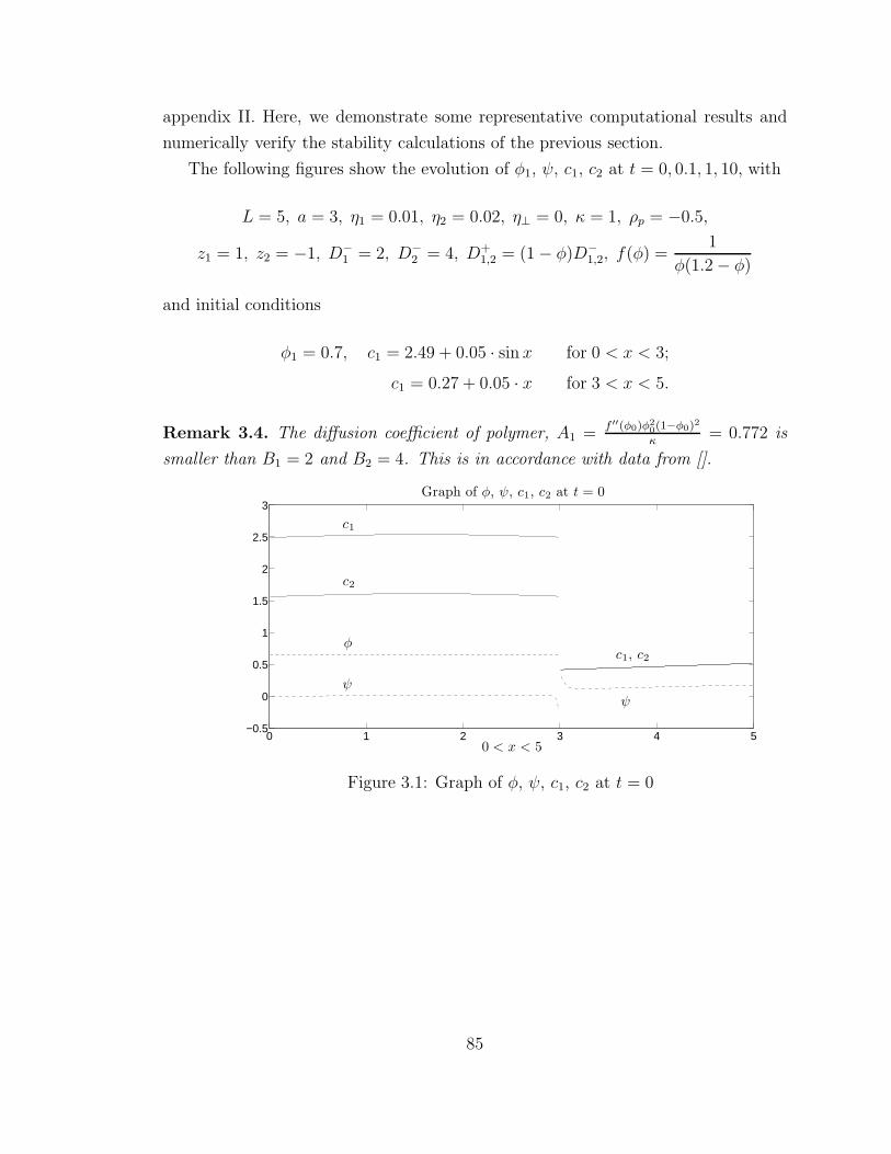
appendix II. Here, we demonstrate some representative computational results and
numerically verify the stability calculations of the previous section.
The following figures show the evolution of φ1, ψ, c1, c2 at t = 0, 0.1, 1, 10, with
L = 5, a = 3, η1 = 0.01, η2 = 0.02, η⊥ = 0, κ = 1, ρp = −0.5,
z1 = 1, z2 = −1, D−1 = 2, D−
2 = 4, D+1,2 = (1− φ)D−
1,2, f(φ) =1
φ(1.2− φ)
and initial conditions
φ1 = 0.7, c1 = 2.49 + 0.05 · sin x for 0 < x < 3;
c1 = 0.27 + 0.05 · x for 3 < x < 5.
Remark 3.4. The diffusion coefficient of polymer, A1 =f ′′(φ0)φ20(1−φ0)
2
κ= 0.772 is
smaller than B1 = 2 and B2 = 4. This is in accordance with data from [].
0 1 2 3 4 5−0.5
0
0.5
1
1.5
2
2.5
3Graph of φ, ψ, c1, c2 at t = 0
0 < x < 5
c1
φ
ψ
c1, c2
c2
ψ
Figure 3.1: Graph of φ, ψ, c1, c2 at t = 0
85
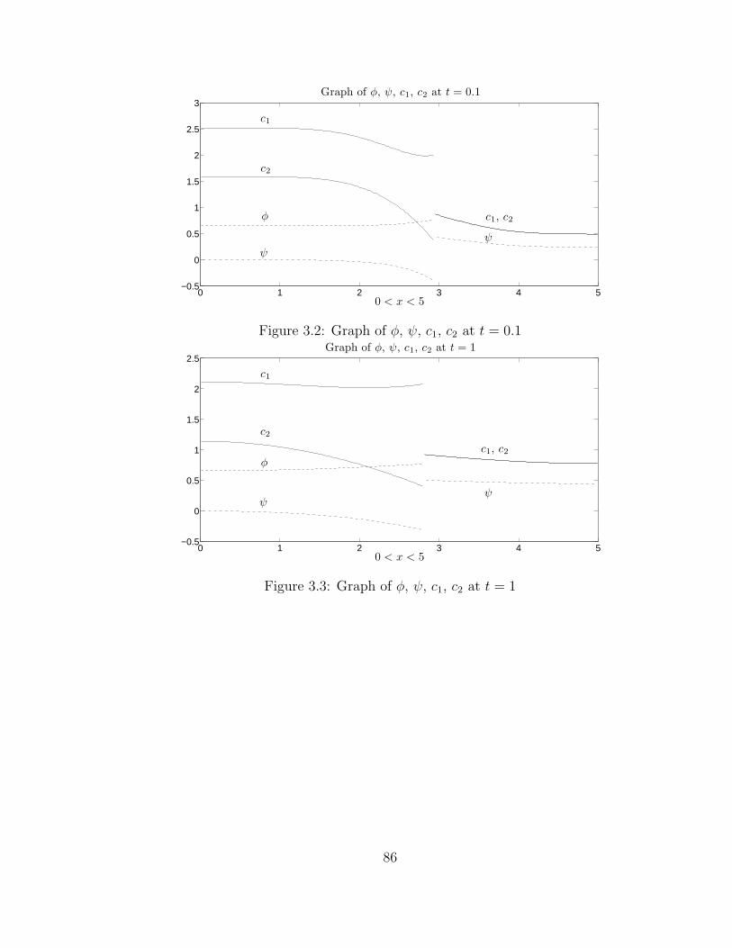
0 1 2 3 4 5−0.5
0
0.5
1
1.5
2
2.5
3Graph of φ, ψ, c1, c2 at t = 0.1
0 < x < 5
c1
c2
ψ
c1, c2φ
ψ
Figure 3.2: Graph of φ, ψ, c1, c2 at t = 0.1
0 1 2 3 4 5−0.5
0
0.5
1
1.5
2
2.5
0 < x < 5
Graph of φ, ψ, c1, c2 at t = 1
c1
c1, c2
c2
φ
ψψ
Figure 3.3: Graph of φ, ψ, c1, c2 at t = 1
86
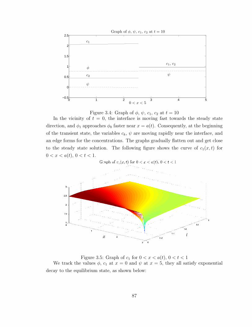
0 1 2 3 4 5−0.5
0
0.5
1
1.5
2
2.5
0 < x < 5
Graph of φ, ψ, c1, c2 at t = 10
c1
c1, c2
c2
ψ
ψ
φ
Figure 3.4: Graph of φ, ψ, c1, c2 at t = 10In the vicinity of t = 0, the interface is moving fast towards the steady state
direction, and φ1 approaches φ0 faster near x = a(t). Consequently, at the beginning
of the transient state, the variables ck, ψ are moving rapidly near the interface, and
an edge forms for the concentrations. The graphs gradually flatten out and get close
to the steady state solution. The following figure shows the curve of c1(x, t) for
0 < x < a(t), 0 < t < 1.
Figure 3.5: Graph of c1 for 0 < x < a(t), 0 < t < 1We track the values φ, c1 at x = 0 and ψ at x = 5, they all satisfy exponential
decay to the equilibrium state, as shown below:
87
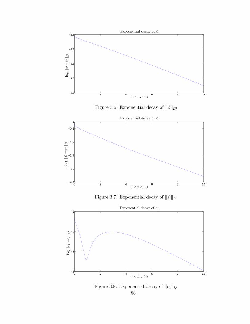
0 2 4 6 8 10−5.5
−4.5
−3.5
−2.5
−1.5
0 < t < 10
log‖φ−φ
0‖
L2
Exponential decay of φ
Figure 3.6: Exponential decay of ‖φ‖L2
0 2 4 6 8 10−4.5
−3.5
−2.5
−1.5
−0.5
0
0 < t < 10
log‖ψ−ψ
0‖
L2
Exponential decay of ψ
Figure 3.7: Exponential decay of ‖ψ‖L2
0 2 4 6 8 10−3
−2
−1
0
0 < t < 10
log‖c1−c0‖
L2
Exponential decay of c1
Figure 3.8: Exponential decay of ‖c1‖L2
88
and the linear approximation shows the rates are
λφ ≈ 0.349, λψ ≈ 0.349, λc ≈ 0.344 (3.300)
which match well with the theoretical value λ ≈ 0.349 derived from (3.269).
89
Bibliography
[1] E. Achilleos, K. Christodoulou, and I. Kevrekidis, A transport model
for swelling of polyelectrolyte gels in simple and complex geometries, Computa-
tional and Theoretical Polymer Science, 11 (2001), pp. 63–80.
[2] A.Yamauchi, Gels Handbook, Vol I, Academic Press, 2001.
[3] L. Bennethum and J. Cushman, Multicomponent, multiphase thermodynam-
ics of swelling porous media with electroquasistatics: I. macroscale field equa-
tions, Transport in porous media, 47 (2002), pp. 309–336.
[4] , Multicomponent, multiphase thermodynamics of swelling porous media
with electroquasistatics: Ii. constitutive theory, Transport in porous media, 47
(2002), pp. 337–362.
[5] M. Calderer, B. Chabaud, S. Lyu, and H. Zhang, Modeling approaches
to the dynamics of hydrogel swelling, Journal of Computational and Theoretical
Nanoscience, 7 (2010), pp. 766–779.
[6] S. De and N. Aluru, A chemo-electro-mechanical mathematical model for
simulation of ph sensitive hydrogels, Mechanics of materials, 36 (2004), pp. 395–
410.
[7] A. Dhanarajan, G. Misra, and R. Siegel, Autonomous chemomechani-
cal oscillations in a hydrogel/enzyme system driven by glucose, The Journal of
Physical Chemistry A, 106 (2002), pp. 8835–8838.
[8] M. Doi, Gel dynamics, J. Phys. Soc. Jpn, 78 (2009), p. 052001.
[9] M. Doi and A. Onuki, Dynamic coupling between stress and composition in
polymer solutions and blends, J. Phys. II France, 2 (1992), pp. 1631–1656.
90
[10] M. Doi and H. See, Introduction to polymer physics, Oxford University Press,
USA, 1996.
[11] A. English, S. Mafe Matoses, J. Manzanares Andreu, X. Yo,
A. Grosberg, and T. Tanaka, Equilibrium swelling properties of polyam-
pholytic hydrogels, Journal of Chemical Physics, (1996).
[12] L. Feng, Y. Jia, X. Chen, X. Li, and L. An, A multiphasic model for the
volume change of polyelectrolyte hydrogels, The Journal of chemical physics, 133
(2010), p. 114904.
[13] P. Flory, Principles of Polymer Chemistry, Cornell U. Press, 1953.
[14] P. Grimshaw, J. Nussbaum, A. Grodzinsky, and M. Yarmush, Kinetics
of electrically and chemically induced swelling in polyelectrolyte gels, The Journal
of Chemical Physics, 93 (1990), p. 4462.
[15] W. Gu, W. Lai, and V. Mow, A mixture theory for charged-hydrated soft
tissues containing multi-electrolytes: passive transport and swelling behaviors,
Journal of biomechanical engineering, 120 (1998), p. 169.
[16] W. Gu WY, Lai and V. Mow, Transport of multi-electrolytes in charged
hydrated biological soft tissues, Transport in Porous Media, 34 (1999), pp. 143–
157.
[17] M.H. Holmes, Introduction to Perturbation Methods, Springer, 1995.
[18] W. Hong, X. Zhao, and Z. Suo, Large deformation and electrochemistry of
polyelectrolyte gels, Journal of the Mechanics and Physics of Solids, 58 (2010),
pp. 558–577.
[19] A. Katchalsky and I.Michaeli, Polyelectrolyte gels in salt solutions, Jour-
nal of Polymer Science, 15 (1955), pp. 69–86.
[20] , Potentiometric titration of polyelectrolyte gels, Journal of Polymer Science,
23 (1957), pp. 683–696.
[21] J.P. Keener, Principles of Applied Mathematics, Perseus Books, 1998.
[22] J. Keener, S. Sircar, and A. Fogelson, Influence of the standard free
energy on swelling kinetics of gels, Physical Review E, 83 (2011), p. 041802.
91
[23] , Kinetics of swelling gels, SIAM Journal on Applied Mathematics, 71
(2011), p. 854.
[24] L. Landau, E. Lifshitz, and L. Pitaevskiı, Electrodynamics of continuous
media, Course of theoretical physics, Butterworth-Heinemann, 1984.
[25] H. Li, R. Luo, and K. Lam, Modeling of ionic transport in electric-stimulus-
responsive hydrogels, Journal of membrane science, 289 (2007), pp. 284–296.
[26] H. Li, T. Ng, Y. Yew, and K. Lam, Modeling and simulation of the
swelling behavior of ph-stimulus-responsive hydrogels, Biomacromolecules, 6
(2005), pp. 109–120.
[27] R. Luo, H. Li, and K. Lam, Modeling and simulation of chemo-electro-
mechanical behavior of ph-electric-sensitive hydrogel, Analytical and Bioanalyt-
ical Chemistry, 389 (2007), pp. 863–873.
[28] G. Misra and R. Siegel, New mode of drug delivery: long term autonomous
rhythmic hormone release across a hydrogel membrane, Journal of controlled
release, 81 (2002), pp. 1–6.
[29] Y. Mori, C. Liu, and R. Eisenberg, A Model of Electrodiffusion and Os-
motic Water Flow and its Energetic Structure, Physica D: Nonlinear Phenom-
ena, 240 (2011), pp. 1835–1852.
[30] J. Ricka and T. Tanaka, Swelling of ionic gels: Quantitative performance
of the donnan theory, Macromolecules, 17 (1984), pp. 2916–2921.
[31] M. Rognes, M. Calderer, and C. Micek, Modelling of and mixed finite
element methods for gels in biomedical applications, SIAM Journal on Applied
Mathematics, 70 (2009), p. 1305.
[32] I. Rubinstein, Electro-diffusion of ions, SIAM studies in applied mathematics,
Society for Industrial and Applied Mathematics, 1990.
[33] R. Aris, Vectors, tensors, and the basic equations of fluid mechanics, Dover,
1989.
[34] Stuart Antman, Nonlinear Problems of Elasticity, Springer, 2006.
92

[35] M. Shibayama and T. Tanaka, Volume phase transition and related phenom-
ena of polymer gels, Responsive gels: volume transitions I, (1993), pp. 1–62.
[36] T. Tanaka, Collapse of gels and the critical endpoint, Physical Review Letters,
12 (1978), pp. 820–823.
[37] , Gels, Scientific American., 244 (1981), p. 110.
[38] T. Tanaka and D. Filmore, Kinetics of selling of gels, J. Chem. Phys., 70
(1979), pp. 1214–1218.
[39] S. Wu, H. Li, J. Chen, and K. Lam, Modeling investigation of hydrogel
volume transition, Macromolecular theory and simulations, 13 (2004), pp. 13–
29.
[40] T. Yamaue, H. Mukai, K. Asaka, and M. Doi, Electrostress diffusion
coupling model for polyelectrolyte gels, Macromolecules, 38 (2005), pp. 1349–
1356.
[41] M. Doi and A. Onuki, Onsager’s variational principle in soft matter dynam-
ics, Non-Equilibrium Soft Matter Physics, 23 (2012), pp. 1–35
[42] Jackson, J.D. and Fox, R.F., Classical electrodynamics, American Journal
of Physics, 67 (1999), pp. 841.
[43] H. Zhang and M. Calderer, Incipient dynamics of swelling of gels, SIAM
Journal on Applied Mathematics, 68 (2008), p. 1641.
[44] X. Zhou, Y. Hon, S. Sun, and A. Mak, Numerical simulation of the steady-
state deformation of a smart hydrogel under an external electric field, Smart
materials and structures, 11 (2002), p. 459.
93
Appendix I: Onsager’s principle
for positive dielectric constant
We consider the system with ionic species, when the dielectric constant being nonzero.
The electrostatic potential ψ no longer satisfies the electroneutral condition (3.46);
instead, it satisfies Poisson equation (3.5). Except this, all the kinematic relations
and constraints, boundary conditions are the same as mentioned in the first two
paragraphs of section 3.3.
Define the potential energy U by
U = U + Eion + Eelec
= U +
∫
Ωt
φ2Wion(ck) +Welecdx+
∫
Rt
Wion(ck) +Welecdx,(A-1)
in which (2.59), (3.1), (3.15) are satisfied. Define the Rayleigh dissipation function
by
W =W +N∑
k=1
∫
Ωt
1
2kBTD
−1k φ2
2ck|uk − v2|2dx
+
N∑
k=1
∫
Rt
1
2kBTD
−1k ck|uk − vf |2dx,
(A-2)
which is similar to (3.126). The stress tensors and body forces are defined by (2.34),
(2.39), (2.41), (2.42), (3.6), (3.8). We state the Onsager’s variational principle for
ǫ 6= 0 as follows.
Theorem A.1. Let φi, vi,f , ck, uk, ψ be smooth functions, φi, ck, ψ satisfy (3.5).
Let U be defined by (A-1), and U be defined through the kinematic relations (2.2),
94
(2.30)-(2.33), (3.121)-(3.122) and (3.5)(taking time derivative). Let
Z ⊂ (C2(Ωt))N+2 × (C2(Rt))
N+1 (A-3)
be a subspace consisting of all elements u1, · · · ,uN ,v1,2,f that (2.3), (2.9), (2.11)-
(2.13), (2.18), (3.123)-(3.124) are satisfied. Suppose, for some u1, · · · ,uN ,v1,2,f ∈Z, (2.4), (2.8) with γ1,2 = 0, (2.34), (2.41), (2.42), (2.39), (3.6), (3.8) and boundary
condition (2.16), (2.44), (2.45), (3.10)-(3.13) are all well defined and satisfied, then
this element u1, · · · ,uN ,v1,2,f minimizes
R = U +W (A-4)
in Z.
Proof. The main steps are similar to the proof of Theorem 2.3. We only present
calculations that differs from the previous one. First, in order to calculate U in Ωt,
we consider the electrostatic energy. Multiply (3.121) by qzkψ, integrate over Ωt,
and take sum from k = 1 to N ,
0 =
∫
Ωt
N∑
k=1
(qzkψ
∂(φ2ck)
∂t+ qzkψ∇ · (φ2ckuk)
)dx
=
N∑
k=1
d
dt
∫
Ωt
qzkψφ2ckdx−N∑
k=1
∫
Ωt
(qzk
∂ψ
∂tφ2ck +∇ · (qzkψφ2ckv1)
)dx
+N∑
k=1
∫
Ωt
qzkψ∇ · (φ2ckuk)dx
=d
dt
∫
Ωt
N∑
k=1
(φ2qzkck)ψdx−∫
Ωt
N∑
k=1
(φ2qzkck)∂ψ
∂tdx
−∫
Ωt
N∑
k=1
(φ2qzkck∇ψ · uk)dx+
∫
Γt
N∑
k=1
qzkψφ2ck(uk − v1) · ndS
=: S1 − S2 −∫
Ωt
N∑
k=1
qzkφ2ck∇ψ · ukdx+
∫
Γt
N∑
k=1
qzkψφ2ck(uk − v1) · ndS
Integrating (3.5) by parts, we derive the following identities to replace S1 and S2 in
95
the above:
S1 =d
dt
∫
Ωt
(−∇ · (ǫ∇ψ)− φ1ρp)ψdx
=d
dt
∫
Ωt
ǫ|∇ψ|2dx− d
dt
∫
Γt
ǫψ∂ψ
∂ndS − d
dt
∫
Ωt
ψφ1ρpdx;
S2 =
∫
Ωt
∂ψ
∂t(−∇ · (ǫ∇ψ)− φ1ρp) dx
=
∫
Ωt
ǫ∇ψ∇∂ψ
∂tdx−
∫
Γt
ǫ∂ψ
∂t
∂ψ
∂ndS −
∫
Ωt
∂ψ
∂tφ1ρpdx,
recall (3.130), and it follows that
d
dt
∫
Ωt
φ2Wion + ǫ|∇ψ|2dx
=
∫
Ωt
N∑
k=1
(φ2ck∇
(∂Wion
∂ck
)· (uk − v2) + qzkφ2ck∇ψ · uk
)+ ǫ∇ψ∇∂ψ
∂tdx
+d
dt
∫
Γt
ǫψ∂ψ
∂ndS +
d
dt
∫
Ωt
ψφ1ρpdx−∫
Ωt
∂ψ
∂tφ1ρpdx+
∫
Γt
−ǫ∂ψ∂t
∂ψ
∂n
+Wionφ2(v1 − v2) · n
+
N∑
k=1
(∂Wion
∂ckφ2ck(v2 − uk) · n− qzkψφ2ck(uk − v1) · n
)dS.
(A-5)
The underlined integrals can be simplified by
d
dt
∫
Ωt
ψφ1ρpdx−∫
Ωt
∂ψ
∂tφ1ρpdx =
∫
Ωt
φ1ρp∇ψ · v1dx = −∫
Ωt
f elec1 · v1dx,
using (2.2)(i = 1) and (3.6). Finally, we subtract the following identity from (A-5),
d
dt
∫
Ωt
1
2ǫ|∇ψ|2dx =
∫
Ωt
1
2
∂ǫ
∂t|∇ψ|2 + ǫ∇ψ · ∇∂ψ
∂t+
∫
Γt
1
2ǫ|∇ψ|2(v1 · n)dS
=
∫
Ωt
1
2∇(∂ǫ
∂φ1
|∇ψ|2)· (φ1v1) + ǫ∇ψ · ∇∂ψ
∂tdx
+
∫
Γt
−1
2
∂ǫ
∂φ1
|∇ψ|2(φ1v1) · n+1
2ǫ|∇ψ|2(v1 · n)dS,
96
to get
d
dt
∫
Ωt
φ2Wion +Welecdx
=
∫
Ωt
N∑
k=1
(φ2ck∇
(∂Wion
∂ck
)· (uk − v2) + qzkφ2ck∇ψ · uk
)
− pelas∆ · v1 − f elec1 · v1dx+
∫
Γt
Wionφ2(v1 − v2) · n
+N∑
k=1
(∂Wion
∂ckφ2ck(v2 − uk) · n− qzkψφ2ck(uk − v1) · n
)
+1
2
∂ǫ
∂φ1|∇ψ|2(φ1v1) · n− ǫ
∂ψ
∂t
∂ψ
∂n− 1
2ǫ|∇ψ|2(v1 · n)dS +
d
dt
∫
Γt
ǫψ∂ψ
∂ndS
(A-6)
For Rt, it is similar to derive
d
dt
∫
Rt
Wion +Welecdx
=
∫
Rt
N∑
k=1
(ck∇
(∂Wion
∂ck
)· uk + qzkck∇ψ · uk
)− kBT∇ck · vfdx
+
∫
Γt
−Wion(v1 · n) +N∑
k=1
(ck∂Wion
∂ck(uk · n) + qzkψck(uk − v1) · n
)(A-7)
+ ǫ∂ψ
∂t
∂ψ
∂n+
1
2ǫ|∇ψ|2(v1 · n)dS − d
dt
∫
Γt
ǫψ∂ψ
∂ndS
+
∫
∂U
N∑
k=1
(−ck
∂Wion
∂ck− qzkψck
)(uk · n)− ǫ
∂ψ
∂t
∂ψ
∂ndS − d
dt
∫
∂U
ǫψ∂ψ
∂ndS.
The integrals on the last line vanish, due to (3.124) and (3.13). Adding (A-6) and
(A-7), we have
d
dt
∫
Ωt
φ2Wion +Welecdx+d
dt
∫
Rt
Wion +Welecdx
=
∫
Ωt
N∑
k=1
(φ2ck∇
(∂Wion
∂ck
)· (uk − v2) + qzkφ2ck∇ψ · uk
)− (pelas∆ + f elec
1 ) · v1dx
+
∫
Rt
N∑
k=1
(ck∇
(∂Wion
∂ck
)· uk + qzkck∇ψ · uk − kBT∇ck · vf
)dx
97
+
∫
Γt
Wion(−φ1v1 − φ2v2) · n+
N∑
k=1
(∂Wion
∂ckφ2ck(v2 − u+
k ) · n
+ ck∂Wion
∂ck(uk · n)) +
N∑
k=1
(−qzkφ2ckψ(u
+k − v1) · n+ qzkckψ(u
−k − v1) · n
)
+1
2
∂ǫ
∂φ1|∇ψ|2(φ1v1) · n−
[ǫ∂ψ
∂t
∂ψ
∂n
]−[1
2ǫ|∇ψ|2(v1 · n)
]dS +
d
dt
∫
Γt
[ǫψ∂ψ
∂n
]dS.
(A-8)
Now we collect (A-1)-(A-4) and (A-8), apply (2.64) and (2.65), to derive R:
R =
∫
Ωt
−∇ · (T1 + Sg) · v1 − (∇ · T2) · v2 +1
2κ|v1 − v2|2
+
N∑
k=1
1
2kBTD
−1k φ2
2ck|uk − v2|2 + (φ1v1 + φ2v2) · ∇pdx
+
∫
Rt
−(∇ · Tf) · vf +
N∑
k=1
1
2kBTD
−1k ck|uk − vf |2 + vf · ∇pdx
+ A in (2.65) + RHS of (A-8).
Due to incompressibility, the last integrand term in Rt can be replaced by a surface
integral term:
∫
Rt
N∑
k=1
−kBT∇ck · vfdx = −∫
Γt
N∑
k=1
kBTck(vf · n)dS.
Now (2.4), (2.8) and (3.136) can be derived from taking partial derivatives. For the
boundary terms, our goal is to reach (2.16), (2.44) and (2.45). Since[ǫψ ∂ψ
∂n
]= 0
from (3.11), the very last integral in (A-8) vanishes. The remaining surface integral
terms of (A-8) are:
Wion(−φ1v1 − φ2v2) · n+N∑
k=1
ck∂Wion
∂ck(φ2v2 − φ2u
+k + u−
k ) · n
−N∑
k=1
kBTck(vf · n)− qzkφ2ckψ(u+k − v1) · n+ qzkckψ(u
−k − v1) · n
+A in (2.65) +1
2
∂ǫ
∂φ1|∇ψ|2(φ1v1) · n−
[ǫ∂ψ
∂t
∂ψ
∂n
]−[1
2ǫ|∇ψ|2(v1 · n)
],
98
We use (2.12), (3.11), (3.123) and the continuity of Wion to eliminate terms on the
first and second lines. Finally, we refer to (3.29)-(3.31), to derive:
1
2
∂ǫ
∂φ1
|∇ψ|2(φ1v1) · n−[ǫ∂ψ
∂t
∂ψ
∂n
]−[1
2ǫ|∇ψ|2(v1 · n)
]=[(Selecn) · v1
].
Consequently, all the boundary integral terms reduce to
A+[(Selecn) · v1
]. (A-9)
Now, similar to the proof of theorem 2.2, it is easy to obtain the boundary conditions
(2.16), (2.44) and (2.45). The proof is finished.
99
Appendix II: Numerical scheme
We turn to the simulation part of our model. With or without ion species, the
equations are defined on moving domains, and we discretize them at the reference
configuration, let 0 < X < a0 be the gel region and a0 < X < L be the fluid
region. We employ uniform grids in (0, a0) and in (a0, L) with grid spacing h and h′,
respectively, and time step length ∆t. Let M , M ′ and Nt be the total numbers of
gel grids, fluid grids and time steps. For a function u(t, X) define in (0, a0)
unm = u(n∆t,mh), D0αhu
nm =
unm+α − unm−α
2αh, (A-1)
D+h u
nm =
unm+1 − unmh
, D−h u
nm =
unm − unm−1
h, (A-2)
and similar in (a0, L) with unm′ , D
0,±h′ .
When there is no ion species in the system, the outside fluid region is trivial, and
(2.67)-(2.79) is simplified to (2.82)-(2.83). At the reference configuration,
(η1 ·
vXϕX
)
X
+φ
1− φ
(η2ϕX
·(
φv
1− φ
)
X
)
X
+ (f(φ)− φf ′(φ))X =κvϕX
(1− φ)2, (A-3)
−η⊥v = η1 ·vXϕX
+φ
1− φ
η2ϕX
·(
φv
1− φ
)
X
+ f(φ)− φf ′(φ) at X = a0 (A-4)
in which ϕ = ϕ(t, X), X ∈ (0, a0) is the deformation map, and v = v1 = ϕt,
φ = φ1 = φ0(ϕX)−1. We discretize (A-3) at X = mh, m = 1, · · · ,M − 1:
η1D−h
(D+h vm
D+h ϕ
nm
)+ η2
φnm1− φnm
·D−h
((D+
h ϕnm)
−1 ·D+h
(φnmvm1− φnm
))
+D−h
(f(φnm+0.5)− φnm+0.5f
′(φnm+0.5))=
κvm(1− φnm)
2·D0
hϕnm
(A-5)
100
and (A-4) at X =Mh = a0:
−η⊥vM =η1D−h
(D−h vM
D−h ϕ
nM
)+ η2
φnM1− φnM
· (D−h ϕ
nM)−1 ·D−
h
(φnMvM1− φnM
)
+ f(φnM−0.5)− f ′(φnM−0.5)
(A-6)
in which
vm =ϕn+1m − ϕnm
∆t, φnm−0.5 =
(φ0)m−0.5
D00.5hϕ
nm−0.5
, φm =1
2(φm−0.5 + φm+0.5), (A-7)
some terms at X = Mh are approximated by those at X = (M − 2)h and X =
(M − 1)h. It is possible to maintain the energy dissipation identity
d
dt
∫ a
0
f(φ)dx = −∫ a
0
(2∑
i=1
ηi|vi,x|2 + κ|v1 − v2|2)dx− η⊥ω
2∣∣x=a
= −∫ a
0
(η1 |vx|2 + η2
∣∣∣∣(
φv
1− φ
)
x
∣∣∣∣2
+κv2
(1− φ)2
)dx− η⊥v
2∣∣x=a
(A-8)
after the discretization, if we express the energy derivative by
f ′(φnm) =
f(φn+1m )−f(φnm)
φn+1m −φnm
if φn+1m 6= φnm;
f ′(φ), φ = φnm if φn+1m = φnm.
(A-9)
In fact, multiply (A-5) by vm and integrate by parts, using (A-6), the only pivotal
part is to maintain
d
dt
∫ a0
0
f(φ)ϕXdX =
∫ a0
0
v (f(φ)− φf ′(φ))X dX (A-10)
at the discrete level. If φn+1m = φnm, there is no problem for this m. For convenience,
we assume equality does not occur, then
M−1∑
m=1
vm ·D−h
(f(φnm+0.5)− φnm+0.5f
′(φnm+0.5))
− vMh
(f(φnM−0.5)− φnM−0.5f
′(φnM−0.5))
101
=−M−1∑
m=0
D+h vm ·
(f(φnm+0.5)− φnm+0.5f
′(φnm+0.5))
=−M−1∑
m=0
D+h vm · f(φnm+0.5) +
M−1∑
m=0
1
∆t
(D+h ϕ
n+1m
D+h ϕ
nm
− 1
)(φ0)m+0.5f
′(φnm+0.5)
=−M−1∑
m=0
D+h vm · f(φnm+0.5)
+1
∆t
M−1∑
m=0
D+h ϕ
n+1m ·
(1
D+h ϕ
nm
− 1
D+h ϕ
n+1m
)(φ0)m+0.5f
′(φnm+0.5)
=− 1
∆t
M−1∑
m=0
(D+h ϕ
n+1m+1 −D+
h ϕnm+1)f(φ
nm+0.5)
− 1
∆t
M−1∑
m=0
D+h ϕ
n+1m ·
(f(φn+1
m+0.5)− f(φnm+0.5))
=− 1
∆t
M−1∑
m=0
(D+h ϕ
n+1m f(φn+1
m+0.5)−D+h ϕ
nmf(φ
nm+0.5)
), (A-11)
the boundary terms on the first line cancel with the ones in (A-6), and the energy
dissipation is guaranteed.
Now consider the model with ion species. We have simplified the equations as
(3.163)-(3.174). At the reference configuration, introduce new variables
uk =
ck · (ϕX − φ0) when 0 < X < a0;
ck · L−aL−a0
when a0 < X < L.(A-12)
for k-th ion. The constitutive equations for uk can be written in divergence form,
hence we apply the finite volume method for uk. In (0, a0), the diffusion equations
and neutrality equations
(uk)t =
(vuk
ϕX − φ0
)
X
+
(Dk
ϕX
(uk
ϕX − φ0
)
X
+DkzkψXϕX
· ukϕX − φ0
)
X
, (A-13)
N∑
k=1
zkuk + φ0ρp = 0, (A-14)
102
are discretized at 0.5h, · · · , (M − 1.5)h in the following manner:
(uk)n+1m−0.5 − (uk)
nm−0.5
∆t= (jk)
n+1m − (jk)
n+1m−1, h · (jk)n+1
m =
vm(uk)n+1m
D+h ϕ
nm − (φ0)m
+(Dk)mD+h ϕ
nm
D00.5h
((uk)
n+1m
D00.5hϕ
nm − (φ0)m
)+
(Dk)mzk(uk)n+1m D0
0.5hψn+1m
D+h ϕ
nm
(D+h ϕ
nm − (φ0)m
) ,
(A-15)
N∑
k=1
zk(uk)n+1m−0.5 + (φ0)m−0.5ρp = 0. (A-16)
Here, (jk)m is the flux at X = mh, m = 1, · · · ,M − 1, (jk)0 = 0, Dk may be non-
constant, (uk)n+1m is the average of (uk)
n+1m−0.5 and (uk)
n+1m+0.5, the neutrality equation
at (M − 0.5)h is also required. We use the implicit scheme to solve for un+1 and
ψn+1, which has two advantages: first, the neutrality constraint must be satisfied at
t = (n+ 1)∆t, it is very difficult to find an explicit scheme which has such property,
if the dielectric constant becomes positive hence the neutrality constraint becomes
Poisson equation, the explicit scheme cannot work out; second, the implicit scheme
is less restrictive on the size of ∆t compared to the explicit scheme, which is very
beneficial when we choose small h. Also, notice that we do not use the fully back-
ward scheme: while applying Newton’s method to solve the nonlinear equations, it
is technically more convenient to use ϕn in the diffusion equations.
The rightmost grid in the gel region is combined with the leftmost grid in the
fluid region, this may avoid the interface flux condition. We have:
(uk)n+1M−0.5 − (uk)
nM−0.5
∆t+
(uk)n+10.5′ − (uk)
n0.5′
∆t= (jk)
n+11′ − (jk)
n+1m−1, h′ · (jk)n+1
m′ =
L−Xm′
L− a0vM(uk)
n+1m′ + (Dk)m′
(L− a0L− a
)2 (D0
0.5h′(uk)n+1m′ + (uk)
n+1m′ zkD
00.5h′ψ
n+1m′
),
in which Xm′ = a0 +mh′, a = ϕnM , (uk)n+1m′ =
1
2
((uk)
n+1(m−0.5)′ + (uk)
n+1(m+0.5)′
).
(A-17)
The diffusion equations and neutrality equations are similar in (a0, L):
(uk)t = v(a0) ·(uk ·
L−X
L− a
)
X
+
(L− a0L− a
)2
(Dk(uk)X +DkukzkψX)X , (A-18)
103
N∑
k=1
zkuk = 0. (A-19)
Accordingly, at a0 + 1.5h′, · · · , a0 + (M − 0.5)h′, we have
(uk)n+1(m−0.5)′ − (uk)
n(m−0.5)′
∆t= (jk)
n+1m′ − (jk)
n+1(m−1)′ , (A-20)
N∑
k=1
zk(uk)n+1(m−0.5)′ = 0. (A-21)
Here, (jk)m′ is defined in (A-17), (jk)n+1M ′ = 0, and the neutrality equation at a0+0.5h′
is also required. For interface conditions, we use (uk)n+1m−0.5, (uk)
n+10.5′ and ψn+1
m−0.5, ψn+10.5′
to represent the corresponding values at X = a0. The discretizations are the same
as above, we only list the equations at the reference configuration:
ln
(u+k
ϕX − φ0
)− ln
(u−k · L− a0
L− a
)+ zk [ψ] = 0, (A-22)
−η⊥v =η1vXϕX
+φ
1− φ
η2ϕX
(φv
1− φ
)
X
+ f(φ)− φf ′(φ)
−N∑
k=1
(u+k
ϕX − φ0− u−k · L− a0
L− a
).
(A-23)
Finally, we have the ionic version of the momentum equation for which
− φρp1 − φ
ψX ≈ − φnmρp1 − φnm
D00.5hψ
n+1m
is added to the left hand side of (A-5). The energy dissipation identity with ion
species is difficult to maintain, mainly because the diffusion equations and the mo-
mentum equation are discretized at different locations, and the interface conditions
are difficult to handle. We do not expect this property in the ionic situation.
104