Characterization and Analysis of theFuselage of the Clipperspirit Seaplane

Item Type text; Electronic Thesis

Authors Sangston, Keith David; Avery, Aaron; Peralta, Bolivar; Pichardo,Luis; Van Wormer, Brett

Publisher The University of Arizona.

Rights Copyright © is held by the author. Digital access to this materialis made possible by the University Libraries, University of Arizona.Further transmission, reproduction or presentation (such aspublic display or performance) of protected items is prohibitedexcept with permission of the author.

Download date 09/07/2018 19:09:18

Link to Item http://hdl.handle.net/10150/244753

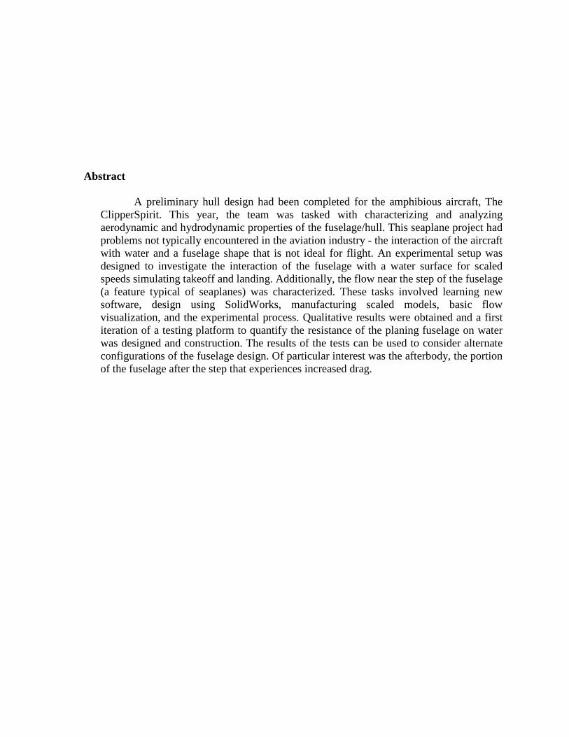
Abstract A preliminary hull design had been completed for the amphibious aircraft, The

ClipperSpirit. This year, the team was tasked with characterizing and analyzing aerodynamic and hydrodynamic properties of the fuselage/hull. This seaplane project had problems not typically encountered in the aviation industry - the interaction of the aircraft with water and a fuselage shape that is not ideal for flight. An experimental setup was designed to investigate the interaction of the fuselage with a water surface for scaled speeds simulating takeoff and landing. Additionally, the flow near the step of the fuselage (a feature typical of seaplanes) was characterized. These tasks involved learning new software, design using SolidWorks, manufacturing scaled models, basic flow visualization, and the experimental process. Qualitative results were obtained and a first iteration of a testing platform to quantify the resistance of the planing fuselage on water was designed and construction. The results of the tests can be used to consider alternate configurations of the fuselage design. Of particular interest was the afterbody, the portion of the fuselage after the step that experiences increased drag.

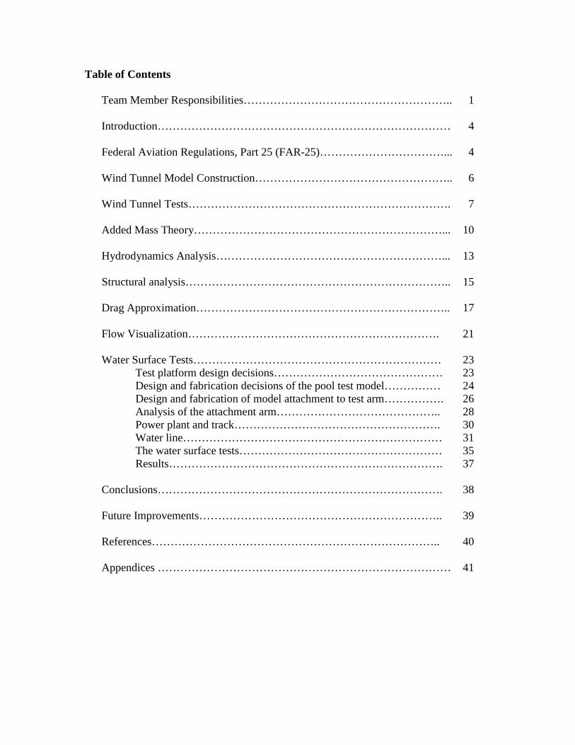
Table of Contents

Team Member Responsibilities……………………………………………….. 1 Introduction…………………………………………………………………… 4 Federal Aviation Regulations, Part 25 (FAR-25)……………………………... 4 Wind Tunnel Model Construction…………………………………………….. 6 Wind Tunnel Tests……………………………………………………………. 7 Added Mass Theory…………………………………………………………... 10 Hydrodynamics Analysis……………………………………………………... 13 Structural analysis…………………………………………………………….. 15 Drag Approximation………………………………………………………….. 17 Flow Visualization…………………………………………………………. Water Surface Tests…………………………………………………………

Test platform design decisions……………………………………… Design and fabrication decisions of the pool test model…………… Design and fabrication of model attachment to test arm……………. Analysis of the attachment arm…………………………………….. Power plant and track………………………………………………. Water line…………………………………………………………… The water surface tests……………………………………………… Results……………………………………………………………….

Conclusions…………………………………………………………………. Future Improvements……………………………………………………….. References…………………………………………………………………..

21

23 23 24 26 28 30 31 35 37

38

39

40

Appendices …………………………………………………………………… 41

1

Team Member Responsibilities Keith Sangston - Team Leader

• FAR-25 Analysis • Wind tunnel model construction • Wind tunnel tests • Water tunnel flow visualization • Design and fabrication of pool fuselage model • Report compilation and editing

Wrote sections… − Federal Aviation Regulations, Part 25 (pp 5-7) − Wind Tunnel Model Construction (pp 7-8) − Wind Tunnel Tests (pp 8-10) − Flow Visualization (pp 22-24) − Design and fabrication of fuselage model (pp 26-27) − Design and fabrication of model attachment to test arm (pp 27-29)

Aaron Avery • Learned the Delftship program • Modeled the fuselage in Delftship • Ran hydrostatic analysis on the hull • Analyzed the results • Cart/Arm construction • Guide/Pulling wires • Design day poster layup • Design day video editing

Wrote sections… − Introduction (p 5) − Hydrodynamics Analysis (pp 14-16) − Conclusions (pp 39-40) − Future Improvements (p 40)

Bolivar Peralta

• Created ANSYS cross section model • Used FAR-25 results to determine forces and deflection on the hull • Validated results from the program using similar structure problem • Water surface test power source • Guide/Pulling wires • Pool fuselage model fabrication

Wrote sections… − Structural Analysis (pp 16-18) − Test platform design decisions (pp 24-25) − Design and fabrication decisions of the pool test model (pp 25-26) − Power plant and track (p 31)

2

Luis Pichardo • Researched water physics • Used added mass theory to obtain resistance • Determined the hydrodynamic force in both horizontal and vertical directions • Water surface test power source • Data acquisition for water surface tests - software familiarization and calibration • Pool test data analysis

Wrote sections… − Added Mass Theory (pp 11-14) − The water surface tests (pp 36-39)

Brett Van Wormer

• Created SolidWorks model • Determined Froude number and scaling • Designed 3D printed model used in wind and water tunnels • Performed fuselage drag analysis and test expectations • Water test attachment arm analysis • Water line estimations for pool tests • Scaled velocity envelope for pool tests • Force estimations for pool tests

Wrote sections… − Drag Approximation (pp 18-22) − Analysis of the attachment arm (pp 29-31) − Water line (pp 32-36)

3

Nomenclature A Horizontal half axis of ellipsoid a Acceleration B Vertical half axis of ellipsoid, area of base of pyramid b Width, span CL Lift coefficient Cd Drag coefficient Cd0 Base drag Cf Skin friction drag coefficient c Chord D Drag force d Diameter F Force Fx Force in x-direction H Hydrodynamic force h Height I Moment of inertia K2 Hull station weighing factor lb Characteristic length M Moment ma Added mass to the system mxx Added mass in the horizontal direction due to a horizontal acceleration mzz Added mass in the vertical direction due to a vertical acceleration N Normal force nw Water reaction divided by seaplane weight P Pressure q Dynamic pressure R Radius, Reaction force Re Reynolds number S, Swet Wetted surface area Sref Reference surface area Ub Velocity of body of interest V Shear force VSO Stalling speed, in knots, flaps extended in landing position with no slipstream effect V∞, v Velocity W Seaplane design landing weight in pounds Γ0 Circulation α Angle of attack β Angle of dead rise at longitudinal station at which load factor is being determined θ Angle λ Length ratio between full size seaplane and model ν Kinematic viscosity ρ Density σ Stress φ Potential function

4

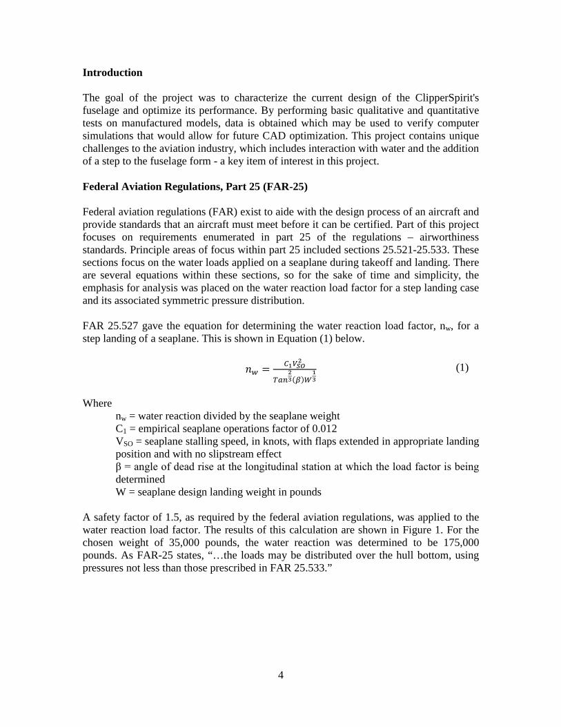
Introduction The goal of the project was to characterize the current design of the ClipperSpirit's fuselage and optimize its performance. By performing basic qualitative and quantitative tests on manufactured models, data is obtained which may be used to verify computer simulations that would allow for future CAD optimization. This project contains unique challenges to the aviation industry, which includes interaction with water and the addition of a step to the fuselage form - a key item of interest in this project. Federal Aviation Regulations, Part 25 (FAR-25) Federal aviation regulations (FAR) exist to aide with the design process of an aircraft and provide standards that an aircraft must meet before it can be certified. Part of this project focuses on requirements enumerated in part 25 of the regulations – airworthiness standards. Principle areas of focus within part 25 included sections 25.521-25.533. These sections focus on the water loads applied on a seaplane during takeoff and landing. There are several equations within these sections, so for the sake of time and simplicity, the emphasis for analysis was placed on the water reaction load factor for a step landing case and its associated symmetric pressure distribution. FAR 25.527 gave the equation for determining the water reaction load factor, nw, for a step landing of a seaplane. This is shown in Equation (1) below.

𝑖𝑤 = 𝐶1𝑉𝑆𝑂2

𝑇𝑎𝑛23(𝛽)𝑊

13

Where nw = water reaction divided by the seaplane weight C1 = empirical seaplane operations factor of 0.012 VSO = seaplane stalling speed, in knots, with flaps extended in appropriate landing

position and with no slipstream effect β = angle of dead rise at the longitudinal station at which the load factor is being

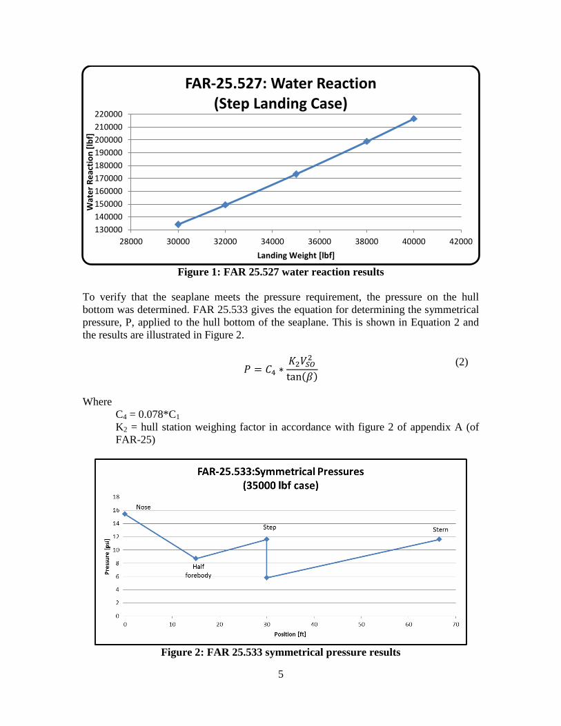
determined W = seaplane design landing weight in pounds A safety factor of 1.5, as required by the federal aviation regulations, was applied to the water reaction load factor. The results of this calculation are shown in Figure 1. For the chosen weight of 35,000 pounds, the water reaction was determined to be 175,000 pounds. As FAR-25 states, “…the loads may be distributed over the hull bottom, using pressures not less than those prescribed in FAR 25.533.”

(1)

5

(2)

Figure 1: FAR 25.527 water reaction results

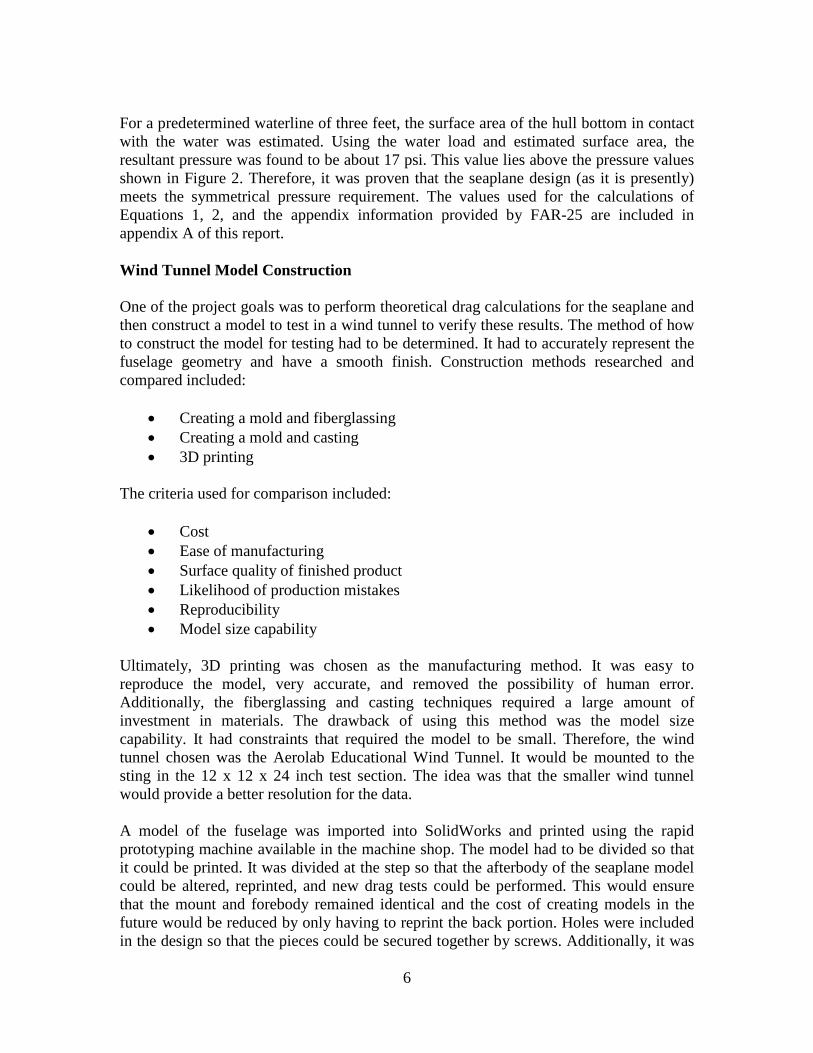
To verify that the seaplane meets the pressure requirement, the pressure on the hull bottom was determined. FAR 25.533 gives the equation for determining the symmetrical pressure, P, applied to the hull bottom of the seaplane. This is shown in Equation 2 and the results are illustrated in Figure 2.

𝑃 = 𝐶4 ∗𝐾2𝑉𝑆𝑂2

tan(𝛽)

Where C4 = 0.078*C1 K2 = hull station weighing factor in accordance with figure 2 of appendix A (of

FAR-25)

Figure 2: FAR 25.533 symmetrical pressure results

130000140000150000160000170000180000190000200000210000220000

28000 30000 32000 34000 36000 38000 40000 42000

Wat

er R

eact

ion

[lbf]

Landing Weight [lbf]

FAR-25.527: Water Reaction (Step Landing Case)

6

For a predetermined waterline of three feet, the surface area of the hull bottom in contact with the water was estimated. Using the water load and estimated surface area, the resultant pressure was found to be about 17 psi. This value lies above the pressure values shown in Figure 2. Therefore, it was proven that the seaplane design (as it is presently) meets the symmetrical pressure requirement. The values used for the calculations of Equations 1, 2, and the appendix information provided by FAR-25 are included in appendix A of this report. Wind Tunnel Model Construction One of the project goals was to perform theoretical drag calculations for the seaplane and then construct a model to test in a wind tunnel to verify these results. The method of how to construct the model for testing had to be determined. It had to accurately represent the fuselage geometry and have a smooth finish. Construction methods researched and compared included:

• Creating a mold and fiberglassing • Creating a mold and casting • 3D printing

The criteria used for comparison included:

• Cost • Ease of manufacturing • Surface quality of finished product • Likelihood of production mistakes • Reproducibility • Model size capability

Ultimately, 3D printing was chosen as the manufacturing method. It was easy to reproduce the model, very accurate, and removed the possibility of human error. Additionally, the fiberglassing and casting techniques required a large amount of investment in materials. The drawback of using this method was the model size capability. It had constraints that required the model to be small. Therefore, the wind tunnel chosen was the Aerolab Educational Wind Tunnel. It would be mounted to the sting in the 12 x 12 x 24 inch test section. The idea was that the smaller wind tunnel would provide a better resolution for the data. A model of the fuselage was imported into SolidWorks and printed using the rapid prototyping machine available in the machine shop. The model had to be divided so that it could be printed. It was divided at the step so that the afterbody of the seaplane model could be altered, reprinted, and new drag tests could be performed. This would ensure that the mount and forebody remained identical and the cost of creating models in the future would be reduced by only having to reprint the back portion. Holes were included in the design so that the pieces could be secured together by screws. Additionally, it was

7

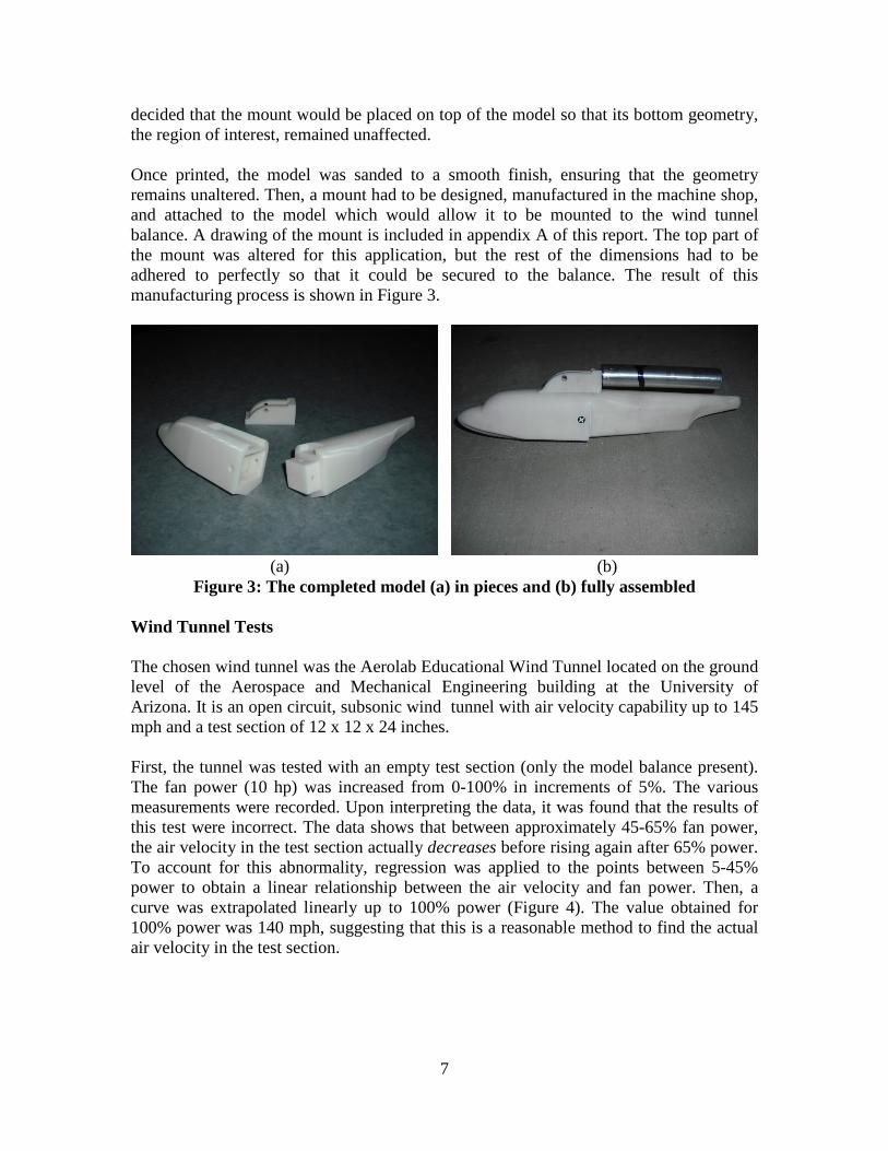
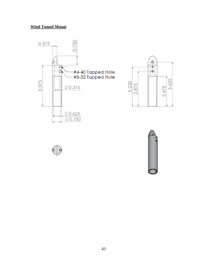
decided that the mount would be placed on top of the model so that its bottom geometry, the region of interest, remained unaffected. Once printed, the model was sanded to a smooth finish, ensuring that the geometry remains unaltered. Then, a mount had to be designed, manufactured in the machine shop, and attached to the model which would allow it to be mounted to the wind tunnel balance. A drawing of the mount is included in appendix A of this report. The top part of the mount was altered for this application, but the rest of the dimensions had to be adhered to perfectly so that it could be secured to the balance. The result of this manufacturing process is shown in Figure 3.

(a) (b)

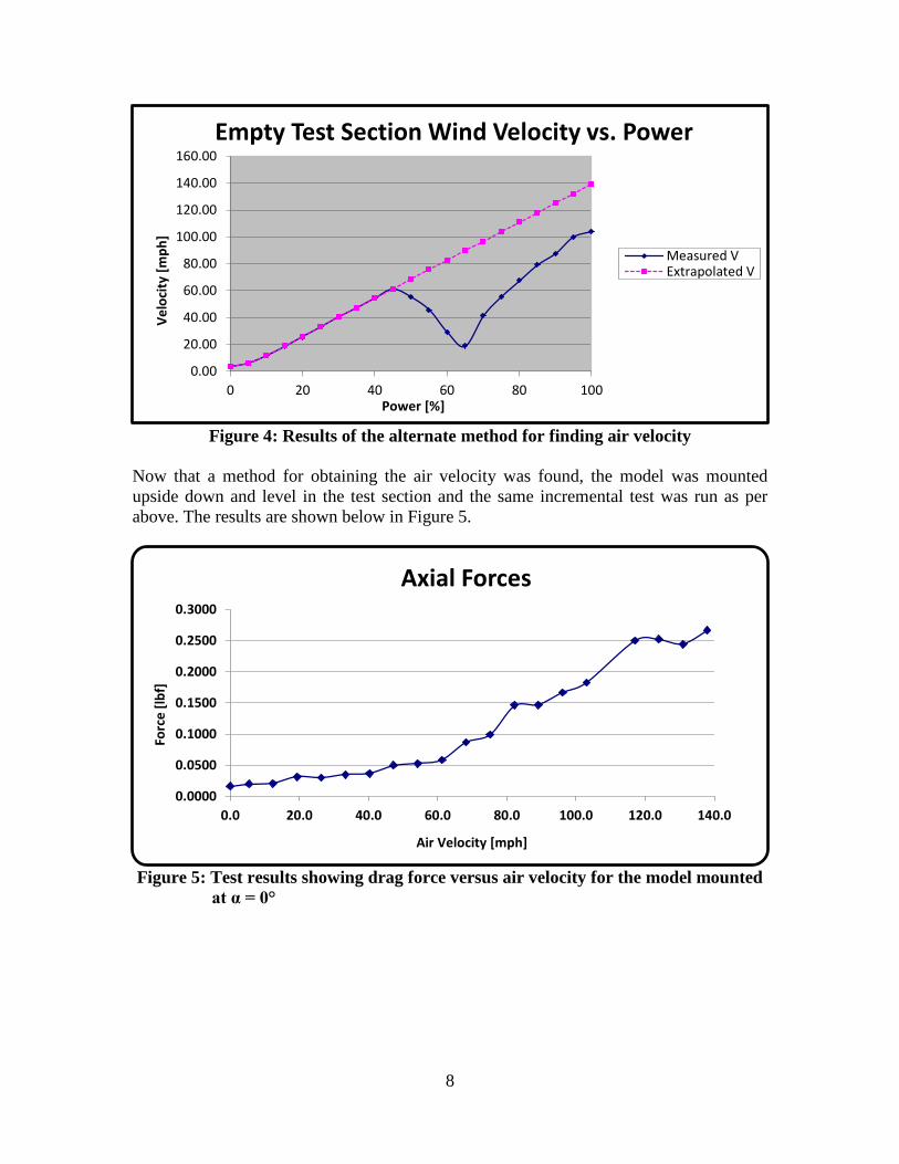
Figure 3: The completed model (a) in pieces and (b) fully assembled Wind Tunnel Tests The chosen wind tunnel was the Aerolab Educational Wind Tunnel located on the ground level of the Aerospace and Mechanical Engineering building at the University of Arizona. It is an open circuit, subsonic wind tunnel with air velocity capability up to 145 mph and a test section of 12 x 12 x 24 inches. First, the tunnel was tested with an empty test section (only the model balance present). The fan power (10 hp) was increased from 0-100% in increments of 5%. The various measurements were recorded. Upon interpreting the data, it was found that the results of this test were incorrect. The data shows that between approximately 45-65% fan power, the air velocity in the test section actually decreases before rising again after 65% power. To account for this abnormality, regression was applied to the points between 5-45% power to obtain a linear relationship between the air velocity and fan power. Then, a curve was extrapolated linearly up to 100% power (Figure 4). The value obtained for 100% power was 140 mph, suggesting that this is a reasonable method to find the actual air velocity in the test section.

8

Figure 4: Results of the alternate method for finding air velocity

Now that a method for obtaining the air velocity was found, the model was mounted upside down and level in the test section and the same incremental test was run as per above. The results are shown below in Figure 5.

Figure 5: Test results showing drag force versus air velocity for the model mounted

at α = 0°

0.00

20.00

40.00

60.00

80.00

100.00

120.00

140.00

160.00

0 20 40 60 80 100

Velo

city

[mph

]

Power [%]

Empty Test Section Wind Velocity vs. Power

Measured VExtrapolated V

0.0000

0.0500

0.1000

0.1500

0.2000

0.2500

0.3000

0.0 20.0 40.0 60.0 80.0 100.0 120.0 140.0

Forc

e [lb

f]

Air Velocity [mph]

Axial Forces

9

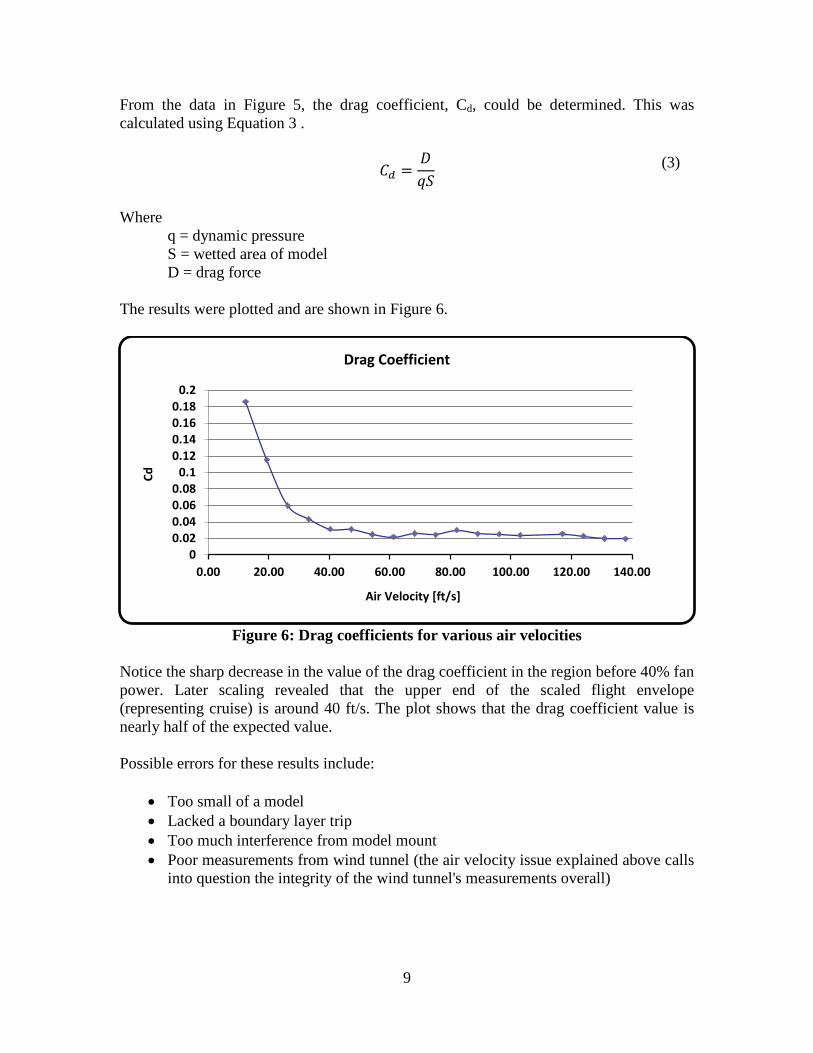
From the data in Figure 5, the drag coefficient, Cd, could be determined. This was calculated using Equation 3 .

𝐶𝑑 =𝐷𝑞𝑆

Where q = dynamic pressure S = wetted area of model D = drag force The results were plotted and are shown in Figure 6.

Figure 6: Drag coefficients for various air velocities

Notice the sharp decrease in the value of the drag coefficient in the region before 40% fan power. Later scaling revealed that the upper end of the scaled flight envelope (representing cruise) is around 40 ft/s. The plot shows that the drag coefficient value is nearly half of the expected value. Possible errors for these results include:

• Too small of a model • Lacked a boundary layer trip • Too much interference from model mount • Poor measurements from wind tunnel (the air velocity issue explained above calls

into question the integrity of the wind tunnel's measurements overall)

00.020.040.060.08

0.10.120.140.160.18

0.2

0.00 20.00 40.00 60.00 80.00 100.00 120.00 140.00

Cd

Air Velocity [ft/s]

Drag Coefficient

(3)

10

Added Mass Theory

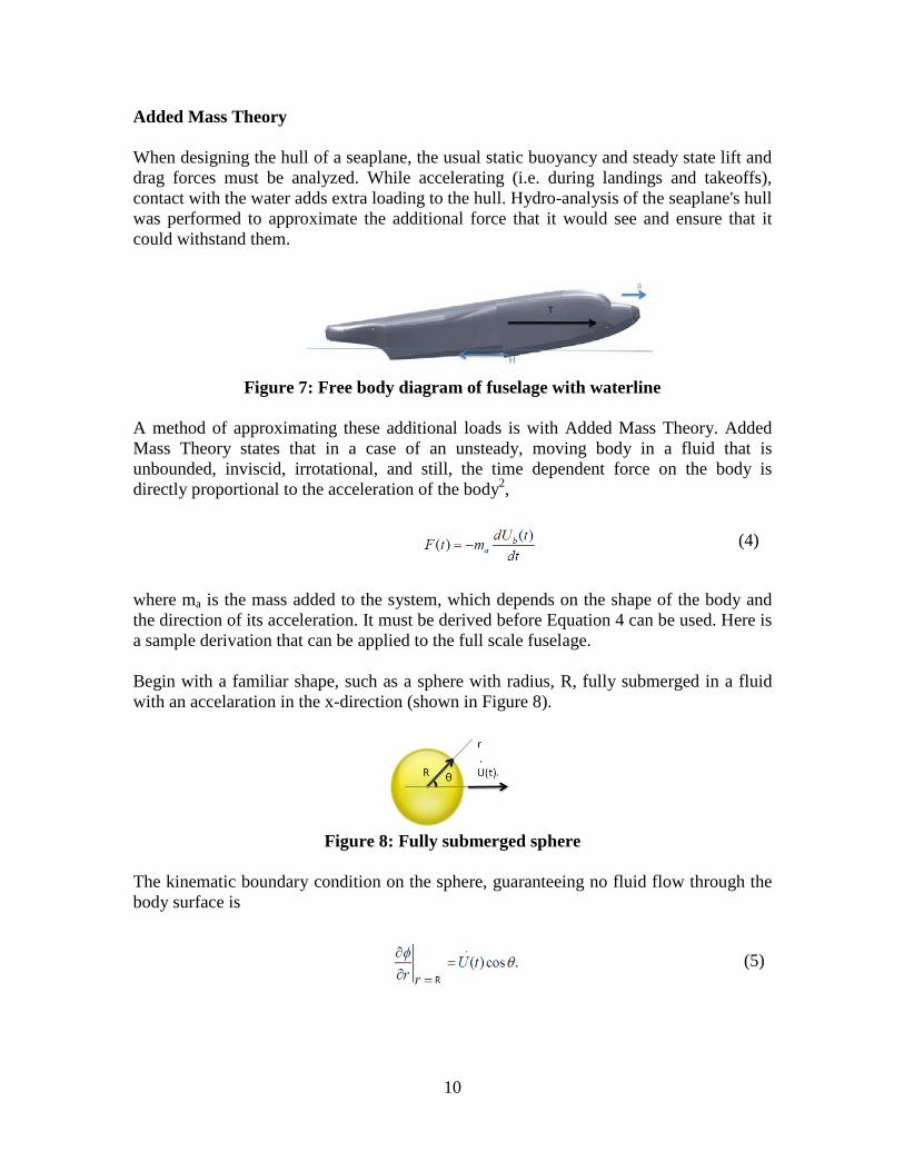
When designing the hull of a seaplane, the usual static buoyancy and steady state lift and drag forces must be analyzed. While accelerating (i.e. during landings and takeoffs), contact with the water adds extra loading to the hull. Hydro-analysis of the seaplane's hull was performed to approximate the additional force that it would see and ensure that it could withstand them.

Figure 7: Free body diagram of fuselage with waterline

A method of approximating these additional loads is with Added Mass Theory. Added Mass Theory states that in a case of an unsteady, moving body in a fluid that is unbounded, inviscid, irrotational, and still, the time dependent force on the body is directly proportional to the acceleration of the body2,

where ma is the mass added to the system, which depends on the shape of the body and the direction of its acceleration. It must be derived before Equation 4 can be used. Here is a sample derivation that can be applied to the full scale fuselage.

Begin with a familiar shape, such as a sphere with radius, R, fully submerged in a fluid with an accelaration in the x-direction (shown in Figure 8).

Figure 8: Fully submerged sphere

The kinematic boundary condition on the sphere, guaranteeing no fluid flow through the body surface is

(4)

(5)

11

(9)

(10)

Then the potential function for the accelerating sphere becomes

The hydrodynamic force on the sphere in Figure 8 is given as a surface integral of pressure around the body. Using the unsteady form of Bernoulli's equation, it is found that the force in the x-direction is

Simplifying Equation 7, the force in the x-direction can be written in terms of volume and fluid density.

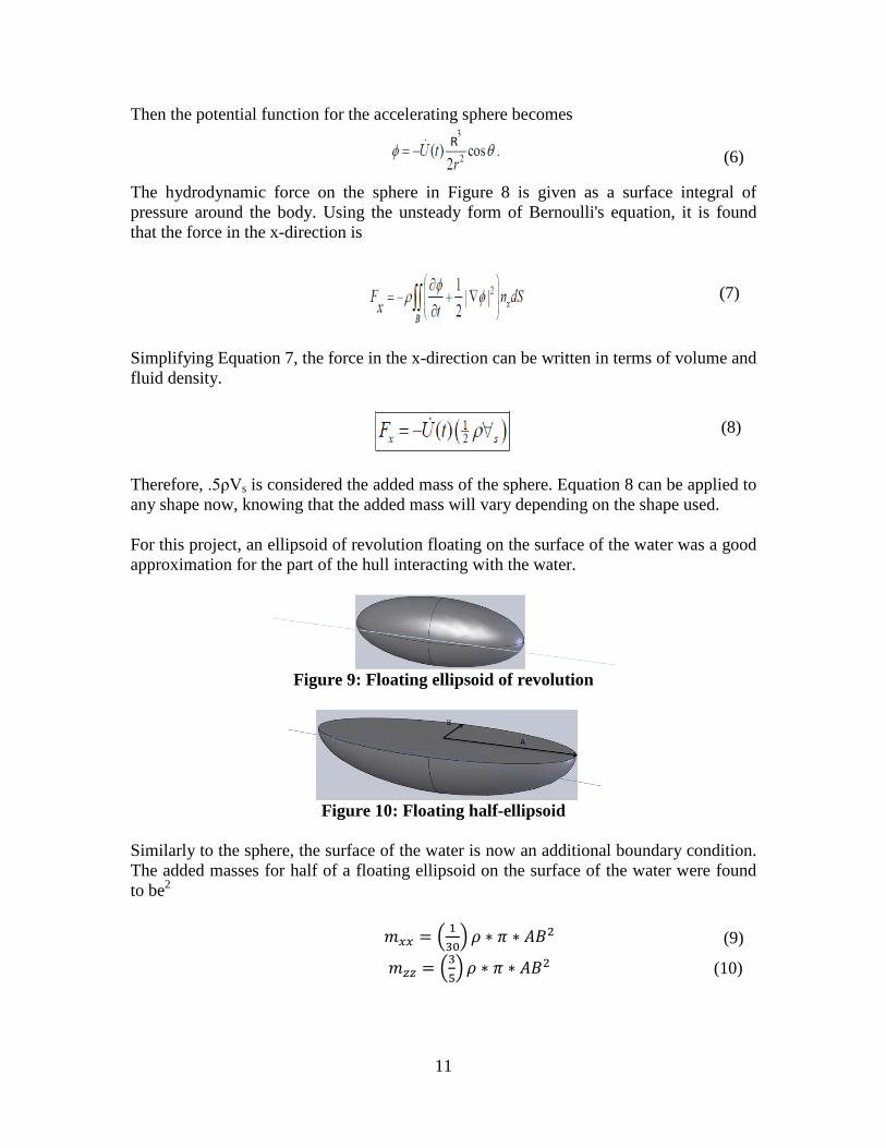
Therefore, .5ρVs is considered the added mass of the sphere. Equation 8 can be applied to any shape now, knowing that the added mass will vary depending on the shape used. For this project, an ellipsoid of revolution floating on the surface of the water was a good approximation for the part of the hull interacting with the water.

Figure 9: Floating ellipsoid of revolution

Figure 10: Floating half-ellipsoid

Similarly to the sphere, the surface of the water is now an additional boundary condition. The added masses for half of a floating ellipsoid on the surface of the water were found to be2

𝑚𝑥𝑥 = � 1

30� 𝜌 ∗ 𝜋 ∗ 𝐴𝐵2

𝑚𝑧𝑧 = �35� 𝜌 ∗ 𝜋 ∗ 𝐴𝐵2

(6)

(7)

(8)

12

(11)

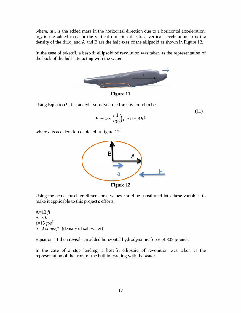
where, mxx is the added mass in the horizontal direction due to a horizontal acceleration, mzz is the added mass in the vertical direction due to a vertical acceleration, ρ is the density of the fluid, and A and B are the half axes of the ellipsoid as shown in Figure 12. In the case of takeoff, a best-fit ellipsoid of revolution was taken as the representation of the back of the hull interacting with the water.

Figure 11

Using Equation 9, the added hydrodynamic force is found to be

𝐻 = 𝑎 ∗ �1

30�𝜌 ∗ 𝜋 ∗ 𝐴𝐵2

where a is acceleration depicted in figure 12.

Figure 12

Using the actual fuselage dimensions, values could be substituted into these variables to make it applicable to this project's efforts. A=12 ft B=3 ft a=15 ft/s2 ρ= 2 slugs/ft3 (density of salt water) Equation 11 then reveals an added horizontal hydrodynamic force of 339 pounds. In the case of a step landing, a best-fit ellipsoid of revolution was taken as the representation of the front of the hull interacting with the water.

B A

a H

13

(12)

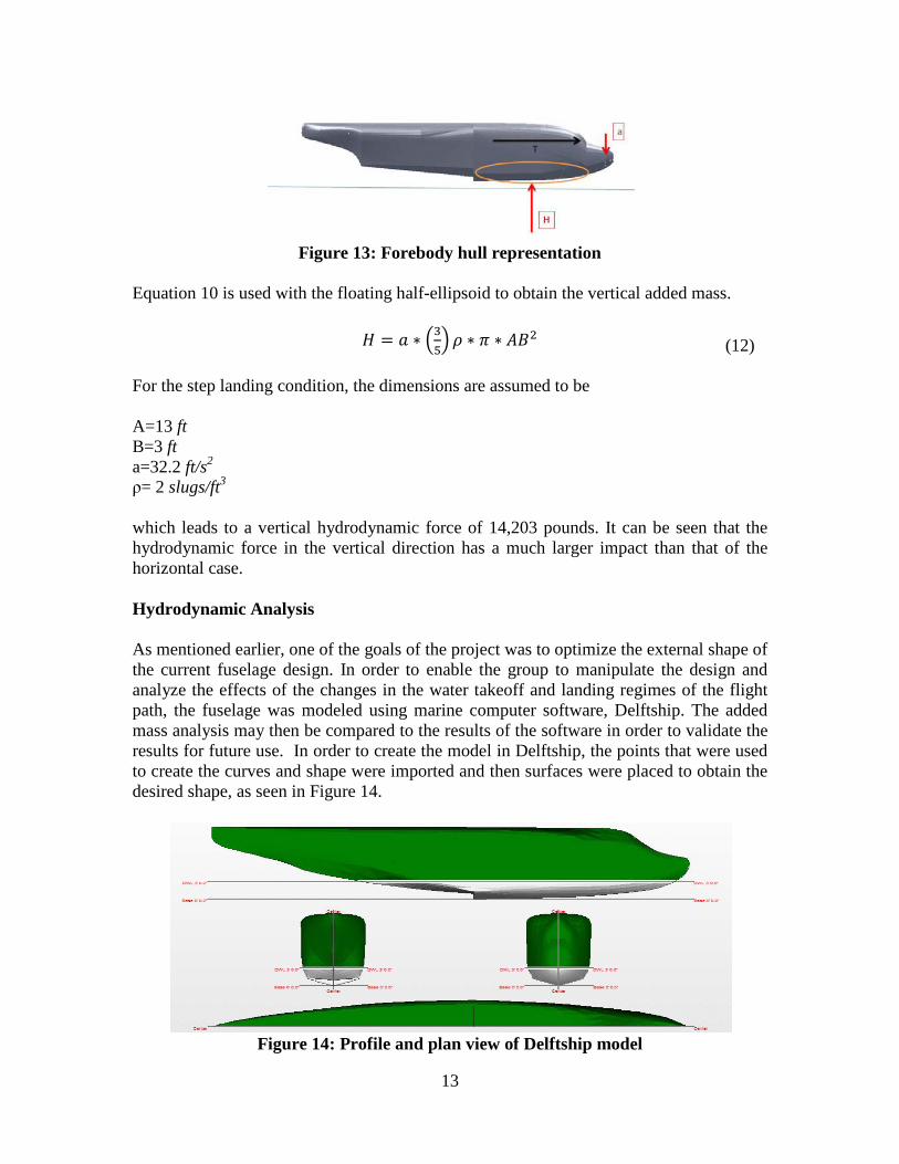
Figure 13: Forebody hull representation

Equation 10 is used with the floating half-ellipsoid to obtain the vertical added mass.

𝐻 = 𝑎 ∗ �3

5� 𝜌 ∗ 𝜋 ∗ 𝐴𝐵2

For the step landing condition, the dimensions are assumed to be A=13 ft B=3 ft a=32.2 ft/s2 ρ= 2 slugs/ft3 which leads to a vertical hydrodynamic force of 14,203 pounds. It can be seen that the hydrodynamic force in the vertical direction has a much larger impact than that of the horizontal case. Hydrodynamic Analysis As mentioned earlier, one of the goals of the project was to optimize the external shape of the current fuselage design. In order to enable the group to manipulate the design and analyze the effects of the changes in the water takeoff and landing regimes of the flight path, the fuselage was modeled using marine computer software, Delftship. The added mass analysis may then be compared to the results of the software in order to validate the results for future use. In order to create the model in Delftship, the points that were used to create the curves and shape were imported and then surfaces were placed to obtain the desired shape, as seen in Figure 14.

Figure 14: Profile and plan view of Delftship model

14

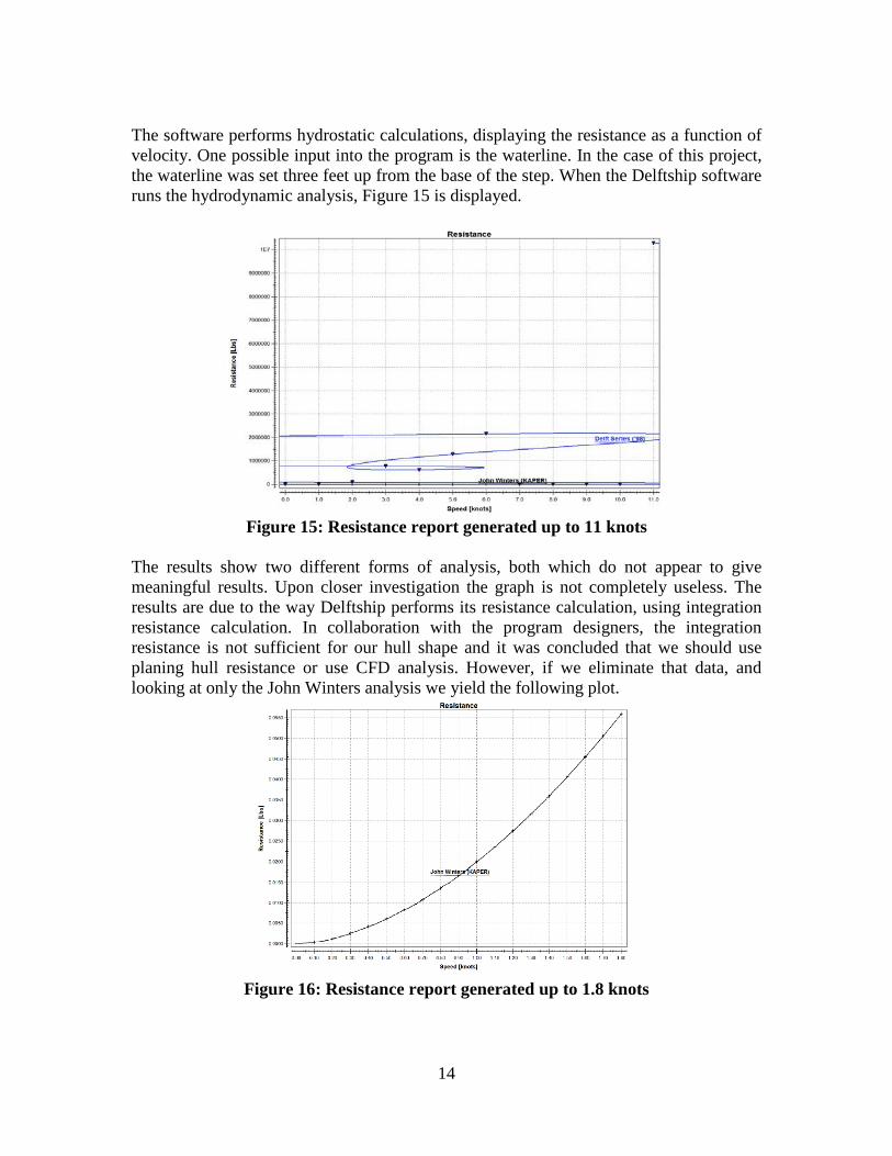
The software performs hydrostatic calculations, displaying the resistance as a function of velocity. One possible input into the program is the waterline. In the case of this project, the waterline was set three feet up from the base of the step. When the Delftship software runs the hydrodynamic analysis, Figure 15 is displayed.

Figure 15: Resistance report generated up to 11 knots

The results show two different forms of analysis, both which do not appear to give meaningful results. Upon closer investigation the graph is not completely useless. The results are due to the way Delftship performs its resistance calculation, using integration resistance calculation. In collaboration with the program designers, the integration resistance is not sufficient for our hull shape and it was concluded that we should use planing hull resistance or use CFD analysis. However, if we eliminate that data, and looking at only the John Winters analysis we yield the following plot.

Figure 16: Resistance report generated up to 1.8 knots

15

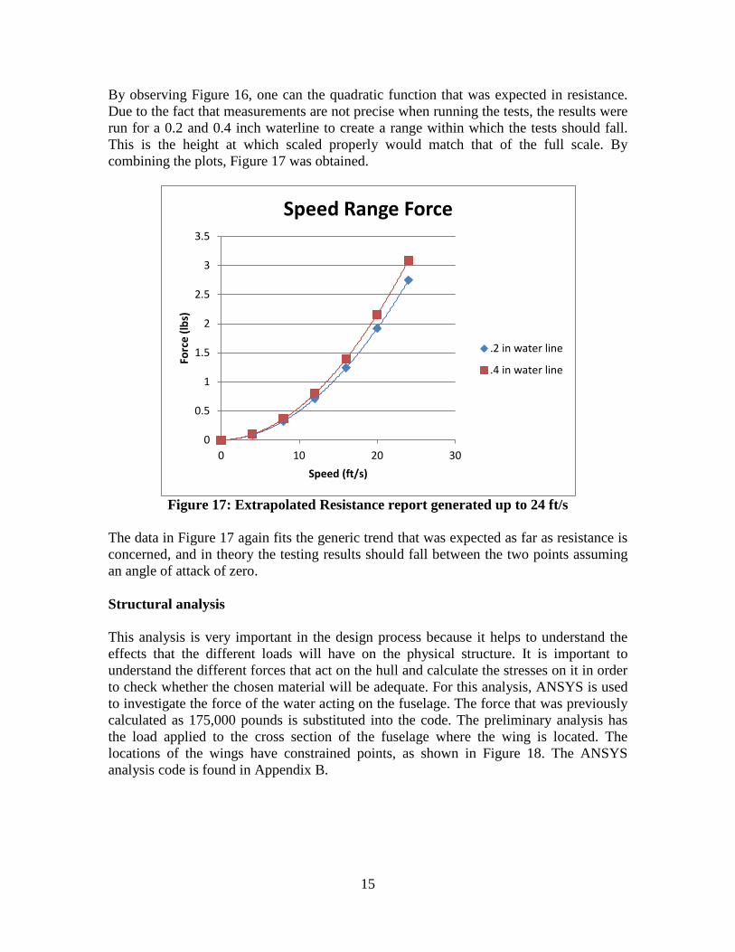
By observing Figure 16, one can the quadratic function that was expected in resistance. Due to the fact that measurements are not precise when running the tests, the results were run for a 0.2 and 0.4 inch waterline to create a range within which the tests should fall. This is the height at which scaled properly would match that of the full scale. By combining the plots, Figure 17 was obtained.

Figure 17: Extrapolated Resistance report generated up to 24 ft/s

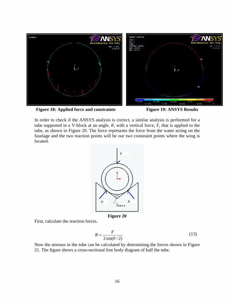
The data in Figure 17 again fits the generic trend that was expected as far as resistance is concerned, and in theory the testing results should fall between the two points assuming an angle of attack of zero. Structural analysis This analysis is very important in the design process because it helps to understand the effects that the different loads will have on the physical structure. It is important to understand the different forces that act on the hull and calculate the stresses on it in order to check whether the chosen material will be adequate. For this analysis, ANSYS is used to investigate the force of the water acting on the fuselage. The force that was previously calculated as 175,000 pounds is substituted into the code. The preliminary analysis has the load applied to the cross section of the fuselage where the wing is located. The locations of the wings have constrained points, as shown in Figure 18. The ANSYS analysis code is found in Appendix B.

0

0.5

1

1.5

2

2.5

3

3.5

0 10 20 30

Forc

e (lb

s)

Speed (ft/s)

Speed Range Force

.2 in water line

.4 in water line

16

Figure 18: Applied force and constraints Figure 19: ANSYS Results In order to check if the ANSYS analysis is correct, a similar analysis is performed for a tube supported in a V-block at an angle, 𝜃, with a vertical force, F, that is applied to the tube, as shown in Figure 20. The force represents the force from the water acting on the fuselage and the two reaction points will be our two constraint points where the wing is located.

Figure 20

First, calculate the reaction forces.

)2/sin(2 θ

FR =

Now the stresses in the tube can be calculated by determining the forces shown in Figure 21. The figure shows a cross-sectional free body diagram of half the tube.

(13)

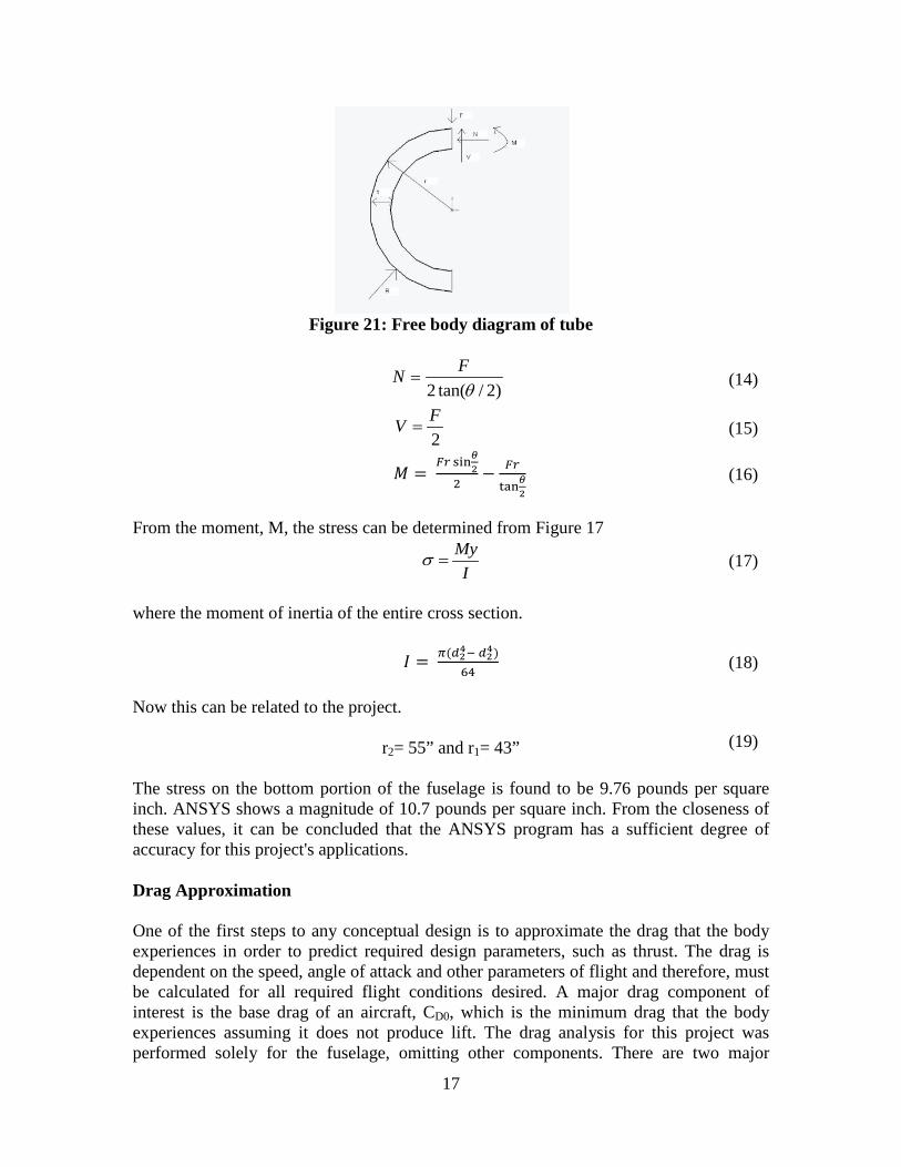
17

Figure 21: Free body diagram of tube

)2/tan(2 θFN =

2FV =

𝑀 = 𝐹𝑟 sin𝜃2

2− 𝐹𝑟

tan𝜃2

From the moment, M, the stress can be determined from Figure 17

IMy

=σ

where the moment of inertia of the entire cross section.

𝐼 = 𝜋(𝑑24− 𝑑24)64

Now this can be related to the project.

r2= 55” and r1= 43”

The stress on the bottom portion of the fuselage is found to be 9.76 pounds per square inch. ANSYS shows a magnitude of 10.7 pounds per square inch. From the closeness of these values, it can be concluded that the ANSYS program has a sufficient degree of accuracy for this project's applications. Drag Approximation One of the first steps to any conceptual design is to approximate the drag that the body experiences in order to predict required design parameters, such as thrust. The drag is dependent on the speed, angle of attack and other parameters of flight and therefore, must be calculated for all required flight conditions desired. A major drag component of interest is the base drag of an aircraft, CD0, which is the minimum drag that the body experiences assuming it does not produce lift. The drag analysis for this project was performed solely for the fuselage, omitting other components. There are two major

(19)

(18)

(17)

(16)

(15)

(14)

18

(20)

(21)

(22)

(24)

(23)

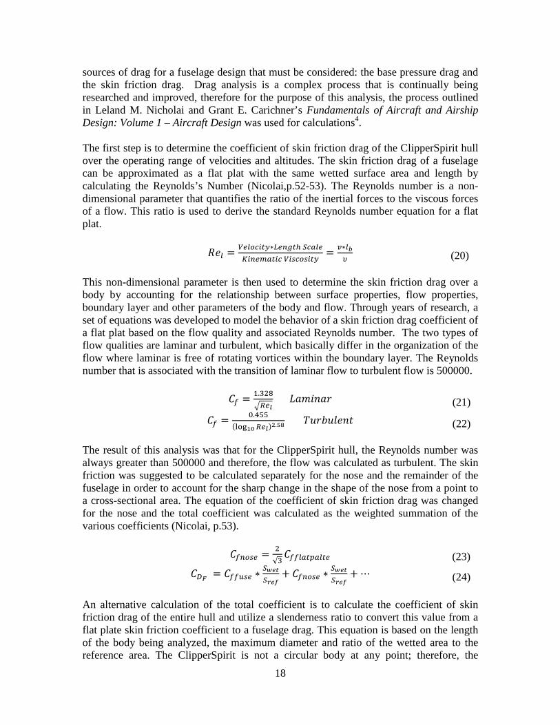
sources of drag for a fuselage design that must be considered: the base pressure drag and the skin friction drag. Drag analysis is a complex process that is continually being researched and improved, therefore for the purpose of this analysis, the process outlined in Leland M. Nicholai and Grant E. Carichner’s Fundamentals of Aircraft and Airship Design: Volume 1 – Aircraft Design was used for calculations4. The first step is to determine the coefficient of skin friction drag of the ClipperSpirit hull over the operating range of velocities and altitudes. The skin friction drag of a fuselage can be approximated as a flat plat with the same wetted surface area and length by calculating the Reynolds’s Number (Nicolai,p.52-53). The Reynolds number is a non-dimensional parameter that quantifies the ratio of the inertial forces to the viscous forces of a flow. This ratio is used to derive the standard Reynolds number equation for a flat plat.

𝑅𝑒𝑙 = 𝑉𝑒𝑙𝑜𝑐𝑖𝑡𝑦∗𝐿𝑒𝑛𝑔𝑡ℎ 𝑆𝑐𝑎𝑙𝑒𝐾𝑖𝑛𝑒𝑚𝑎𝑡𝑖𝑐 𝑉𝑖𝑠𝑐𝑜𝑠𝑖𝑡𝑦

= 𝑣∗𝑙𝑏𝜐

This non-dimensional parameter is then used to determine the skin friction drag over a body by accounting for the relationship between surface properties, flow properties, boundary layer and other parameters of the body and flow. Through years of research, a set of equations was developed to model the behavior of a skin friction drag coefficient of a flat plat based on the flow quality and associated Reynolds number. The two types of flow qualities are laminar and turbulent, which basically differ in the organization of the flow where laminar is free of rotating vortices within the boundary layer. The Reynolds number that is associated with the transition of laminar flow to turbulent flow is 500000.

𝐶𝑓 = 1.328�𝑅𝑒𝑙

𝐿𝑎𝑚𝑖𝑖𝑎𝑟

𝐶𝑓 = 0.455(log10 𝑅𝑒𝑙)2.58 𝑇𝑢𝑟𝑏𝑢𝑙𝑒𝑖𝑡

The result of this analysis was that for the ClipperSpirit hull, the Reynolds number was always greater than 500000 and therefore, the flow was calculated as turbulent. The skin friction was suggested to be calculated separately for the nose and the remainder of the fuselage in order to account for the sharp change in the shape of the nose from a point to a cross-sectional area. The equation of the coefficient of skin friction drag was changed for the nose and the total coefficient was calculated as the weighted summation of the various coefficients (Nicolai, p.53).

𝐶𝑓𝑛𝑜𝑠𝑒 = 2√3𝐶𝑓𝑓𝑙𝑎𝑡𝑝𝑎𝑙𝑡𝑒

𝐶𝐷𝐹 = 𝐶𝑓𝑓𝑢𝑠𝑒 ∗𝑆𝑤𝑒𝑡𝑆𝑟𝑒𝑓

+ 𝐶𝑓𝑛𝑜𝑠𝑒 ∗𝑆𝑤𝑒𝑡𝑆𝑟𝑒𝑓

+ ⋯

An alternative calculation of the total coefficient is to calculate the coefficient of skin friction drag of the entire hull and utilize a slenderness ratio to convert this value from a flat plate skin friction coefficient to a fuselage drag. This equation is based on the length of the body being analyzed, the maximum diameter and ratio of the wetted area to the reference area. The ClipperSpirit is not a circular body at any point; therefore, the

19

(26)

(25)

(27)

(28) (29)

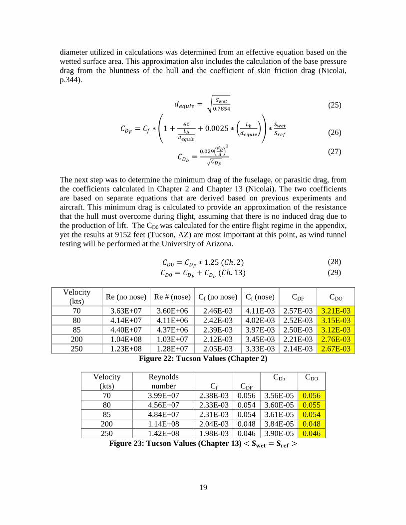
diameter utilized in calculations was determined from an effective equation based on the wetted surface area. This approximation also includes the calculation of the base pressure drag from the bluntness of the hull and the coefficient of skin friction drag (Nicolai, p.344).

𝑑𝑒𝑞𝑢𝑖𝑣 = � 𝑆𝑤𝑒𝑡0.7854

𝐶𝐷𝐹 = 𝐶𝑓 ∗ �1 + 60𝐿𝑏

𝑑𝑒𝑞𝑢𝑖𝑣

+ 0.0025 ∗ � 𝐿𝑏𝑑𝑒𝑞𝑢𝑖𝑣

�� ∗ 𝑆𝑤𝑒𝑡𝑆𝑟𝑒𝑓

𝐶𝐷𝑏 =0.029�

𝑑𝑏𝑑 �

3

�𝐶𝐷𝐹

The next step was to determine the minimum drag of the fuselage, or parasitic drag, from the coefficients calculated in Chapter 2 and Chapter 13 (Nicolai). The two coefficients are based on separate equations that are derived based on previous experiments and aircraft. This minimum drag is calculated to provide an approximation of the resistance that the hull must overcome during flight, assuming that there is no induced drag due to the production of lift. The CD0 was calculated for the entire flight regime in the appendix, yet the results at 9152 feet (Tucson, AZ) are most important at this point, as wind tunnel testing will be performed at the University of Arizona.

𝐶𝐷0 = 𝐶𝐷𝐹 ∗ 1.25 (𝐶ℎ. 2) 𝐶𝐷0 = 𝐶𝐷𝐹 + 𝐶𝐷𝑏 (𝐶ℎ. 13)

Velocity

(kts) Re (no nose) Re # (nose) Cf (no nose) Cf (nose) CDF CDO

70 3.63E+07 3.60E+06 2.46E-03 4.11E-03 2.57E-03 3.21E-03 80 4.14E+07 4.11E+06 2.42E-03 4.02E-03 2.52E-03 3.15E-03 85 4.40E+07 4.37E+06 2.39E-03 3.97E-03 2.50E-03 3.12E-03 200 1.04E+08 1.03E+07 2.12E-03 3.45E-03 2.21E-03 2.76E-03 250 1.23E+08 1.28E+07 2.05E-03 3.33E-03 2.14E-03 2.67E-03

Figure 22: Tucson Values (Chapter 2)

Velocity (kts)

Reynolds number Cf CDF

CDb CDO

70 3.99E+07 2.38E-03 0.056 3.56E-05 0.056 80 4.56E+07 2.33E-03 0.054 3.60E-05 0.055 85 4.84E+07 2.31E-03 0.054 3.61E-05 0.054 200 1.14E+08 2.04E-03 0.048 3.84E-05 0.048 250 1.42E+08 1.98E-03 0.046 3.90E-05 0.046

Figure 23: Tucson Values (Chapter 13) < 𝐒𝐰𝐞𝐭 = 𝐒𝐫𝐞𝐟 >

20

(30)

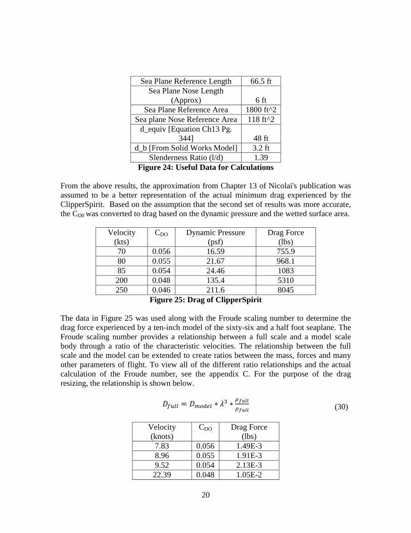
Sea Plane Reference Length 66.5 ft Sea Plane Nose Length

(Approx) 6 ft Sea Plane Reference Area 1800 ft^2

Sea plane Nose Reference Area 118 ft^2 d_equiv [Equation Ch13 Pg.

344] 48 ft d_b [From Solid Works Model] 3.2 ft

Slenderness Ratio (l/d) 1.39 Figure 24: Useful Data for Calculations

From the above results, the approximation from Chapter 13 of Nicolai's publication was assumed to be a better representation of the actual minimum drag experienced by the ClipperSpirit. Based on the assumption that the second set of results was more accurate, the CD0 was converted to drag based on the dynamic pressure and the wetted surface area.

Velocity (kts)

CDO Dynamic Pressure (psf)

Drag Force (lbs)

70 0.056 16.59 755.9 80 0.055 21.67 968.1 85 0.054 24.46 1083 200 0.048 135.4 5310 250 0.046 211.6 8045

Figure 25: Drag of ClipperSpirit The data in Figure 25 was used along with the Froude scaling number to determine the drag force experienced by a ten-inch model of the sixty-six and a half foot seaplane. The Froude scaling number provides a relationship between a full scale and a model scale body through a ratio of the characteristic velocities. The relationship between the full scale and the model can be extended to create ratios between the mass, forces and many other parameters of flight. To view all of the different ratio relationships and the actual calculation of the Froude number, see the appendix C. For the purpose of the drag resizing, the relationship is shown below.

𝐷𝑓𝑢𝑙𝑙 = 𝐷𝑚𝑜𝑑𝑒𝑙 ∗ 𝜆3 ∗𝜌𝑓𝑢𝑙𝑙𝜌𝑓𝑢𝑙𝑙

Velocity (knots)

CDO Drag Force (lbs)

7.83 0.056 1.49E-3 8.96 0.055 1.91E-3 9.52 0.054 2.13E-3 22.39 0.048 1.05E-2

21

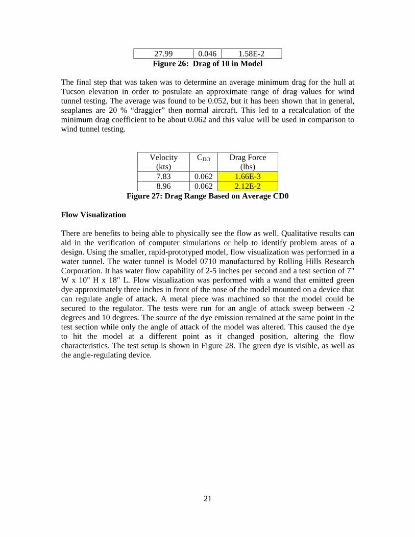
27.99 0.046 1.58E-2 Figure 26: Drag of 10 in Model

The final step that was taken was to determine an average minimum drag for the hull at Tucson elevation in order to postulate an approximate range of drag values for wind tunnel testing. The average was found to be 0.052, but it has been shown that in general, seaplanes are 20 % “draggier” then normal aircraft. This led to a recalculation of the minimum drag coefficient to be about 0.062 and this value will be used in comparison to wind tunnel testing.

Velocity (kts)

CDO Drag Force (lbs)

7.83 0.062 1.66E-3 8.96 0.062 2.12E-2

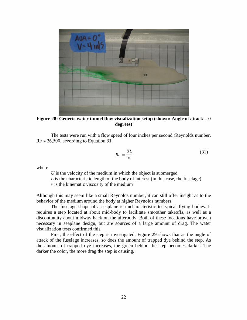
Figure 27: Drag Range Based on Average CD0 Flow Visualization There are benefits to being able to physically see the flow as well. Qualitative results can aid in the verification of computer simulations or help to identify problem areas of a design. Using the smaller, rapid-prototyped model, flow visualization was performed in a water tunnel. The water tunnel is Model 0710 manufactured by Rolling Hills Research Corporation. It has water flow capability of 2-5 inches per second and a test section of 7" W x 10" H x 18" L. Flow visualization was performed with a wand that emitted green dye approximately three inches in front of the nose of the model mounted on a device that can regulate angle of attack. A metal piece was machined so that the model could be secured to the regulator. The tests were run for an angle of attack sweep between -2 degrees and 10 degrees. The source of the dye emission remained at the same point in the test section while only the angle of attack of the model was altered. This caused the dye to hit the model at a different point as it changed position, altering the flow characteristics. The test setup is shown in Figure 28. The green dye is visible, as well as the angle-regulating device.

22

Figure 28: Generic water tunnel flow visualization setup (shown: Angle of attack = 0

degrees) The tests were run with a flow speed of four inches per second (Reynolds number, Re ≈ 26,500, according to Equation 31.

𝑅𝑒 =𝑈𝐿𝜈

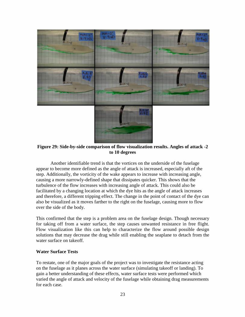
where U is the velocity of the medium in which the object is submerged L is the characteristic length of the body of interest (in this case, the fuselage) ν is the kinematic viscosity of the medium Although this may seem like a small Reynolds number, it can still offer insight as to the behavior of the medium around the body at higher Reynolds numbers. The fuselage shape of a seaplane is uncharacteristic to typical flying bodies. It requires a step located at about mid-body to facilitate smoother takeoffs, as well as a discontinuity about midway back on the afterbody. Both of these locations have proven necessary in seaplane design, but are sources of a large amount of drag. The water visualization tests confirmed this. First, the effect of the step is investigated. Figure 29 shows that as the angle of attack of the fuselage increases, so does the amount of trapped dye behind the step. As the amount of trapped dye increases, the green behind the step becomes darker. The darker the color, the more drag the step is causing.

(31)

23

Figure 29: Side-by-side comparison of flow visualization results. Angles of attack -2

to 10 degrees Another identifiable trend is that the vortices on the underside of the fuselage appear to become more defined as the angle of attack is increased, especially aft of the step. Additionally, the vorticity of the wake appears to increase with increasing angle, causing a more narrowly-defined shape that dissipates quicker. This shows that the turbulence of the flow increases with increasing angle of attack. This could also be facilitated by a changing location at which the dye hits as the angle of attack increases and therefore, a different tripping effect. The change in the point of contact of the dye can also be visualized as it moves farther to the right on the fuselage, causing more to flow over the side of the body. This confirmed that the step is a problem area on the fuselage design. Though necessary for taking off from a water surface, the step causes unwanted resistance in free flight. Flow visualization like this can help to characterize the flow around possible design solutions that may decrease the drag while still enabling the seaplane to detach from the water surface on takeoff. Water Surface Tests To restate, one of the major goals of the project was to investigate the resistance acting on the fuselage as it planes across the water surface (simulating takeoff or landing). To gain a better understanding of these effects, water surface tests were performed which varied the angle of attack and velocity of the fuselage while obtaining drag measurements for each case.

24

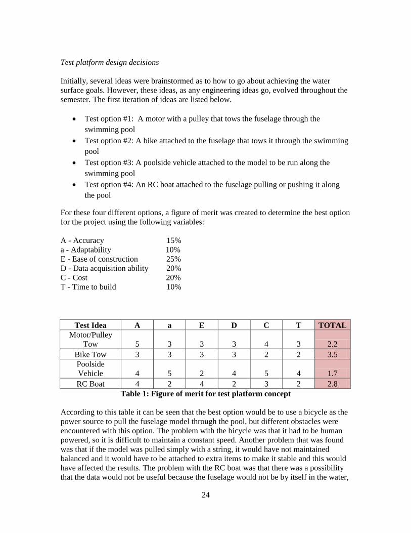
Test platform design decisions Initially, several ideas were brainstormed as to how to go about achieving the water surface goals. However, these ideas, as any engineering ideas go, evolved throughout the semester. The first iteration of ideas are listed below.

• Test option #1: A motor with a pulley that tows the fuselage through the swimming pool

• Test option #2: A bike attached to the fuselage that tows it through the swimming pool

• Test option #3: A poolside vehicle attached to the model to be run along the swimming pool

• Test option #4: An RC boat attached to the fuselage pulling or pushing it along the pool

For these four different options, a figure of merit was created to determine the best option for the project using the following variables: A - Accuracy 15% a - Adaptability 10% E - Ease of construction 25% D - Data acquisition ability 20% C - Cost 20% T - Time to build 10%

Test Idea A a E D C T TOTAL Motor/Pulley

Tow 5 3 3 3 4 3 2.2 Bike Tow 3 3 3 3 2 2 3.5 Poolside Vehicle 4 5 2 4 5 4 1.7 RC Boat 4 2 4 2 3 2 2.8

Table 1: Figure of merit for test platform concept According to this table it can be seen that the best option would be to use a bicycle as the power source to pull the fuselage model through the pool, but different obstacles were encountered with this option. The problem with the bicycle was that it had to be human powered, so it is difficult to maintain a constant speed. Another problem that was found was that if the model was pulled simply with a string, it would have not maintained balanced and it would have to be attached to extra items to make it stable and this would have affected the results. The problem with the RC boat was that there was a possibility that the data would not be useful because the fuselage would not be by itself in the water,

25

there would have been two objects in the water compromising the results for the fuselage itself. Finally it was decided to use a combination of the motor with a pulley and a poolside vehicle. This was the best option because now a constant speed was maintained and the model could be attached to the cart with an adjacent arm. Now the model is sitting in the water by itself and the arm makes easier the job of attaching a force measuring device and also to change its angle of attack. Design and fabrication decisions of the pool test model The final design would incorporate a cart attached to a motor, which would pull it along two guide ropes, while the cart drags the fuselage model attached to a wooden arm along the surface of the water. Now that a testing platform idea was solidified, the pool test model had to be manufactured. This would utilize a different scale (1:33) than the wind and water tunnel model (1:80). In order to meet the requirements, three different options were considered.

• Model building option #1: Send the model to be printed by an external company dedicated to building scale composite material models

• Model building option #2: Print the model with the university’s machine shop 3D printer

• Model building option #3: Build the model using balsa wood

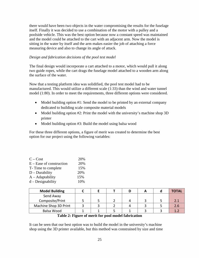
For these three different options, a figure of merit was created to determine the best option for our project using the following variables: C – Cost 20% E – Ease of construction 20% T- Time to complete 15% D – Durability 20% A – Adaptability 15% d – Designability 10%

Model Building C E T D A d TOTAL Send Away

Composite/Print 5 5 2 4 3 5 2.1 Machine Shop 3D Print 3 3 2 4 3 5 2.6

Balsa Wood 1 1 5 1 3 3 1.2 Table 2: Figure of merit for pool model fabrication

It can be seen that our best option was to build the model in the university’s machine shop using the 3D printer available, but this method was constrained by size and time

26

limitations. Consequently, the second option was chosen, which was to send it to a company. The focus then shifted to designing the model so that it attached to the testing platform while adhering to a list of requirements.

• Hollow to reduce weight and permit the placement of objects inside • Manufactured in parts due to machine limitations • Water tight and capable of withstanding forces it would be subjected to during

testing • Manufactured so that the afterbody (a key area of interest of the fuselage shape)

could be swapped with alternate designs without affecting the other components, thereby reducing manufacturing time and cost

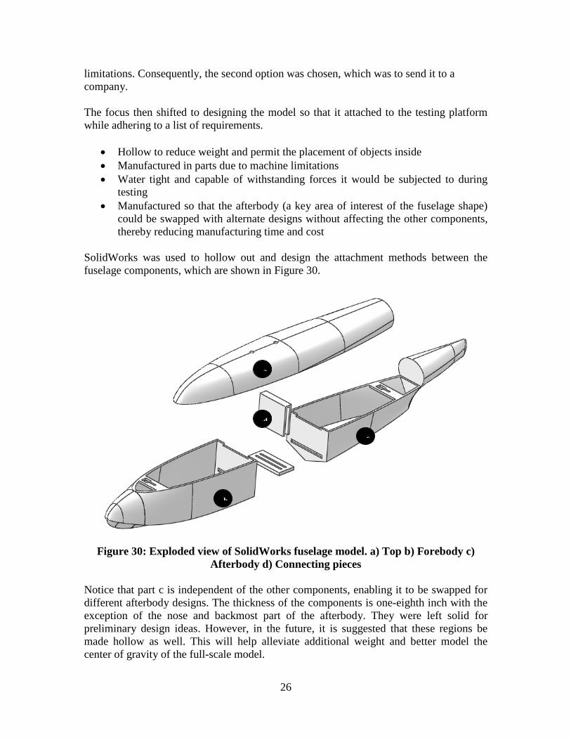
SolidWorks was used to hollow out and design the attachment methods between the fuselage components, which are shown in Figure 30.

Figure 30: Exploded view of SolidWorks fuselage model. a) Top b) Forebody c) Afterbody d) Connecting pieces

Notice that part c is independent of the other components, enabling it to be swapped for different afterbody designs. The thickness of the components is one-eighth inch with the exception of the nose and backmost part of the afterbody. They were left solid for preliminary design ideas. However, in the future, it is suggested that these regions be made hollow as well. This will help alleviate additional weight and better model the center of gravity of the full-scale model.

a

b

c

d

27

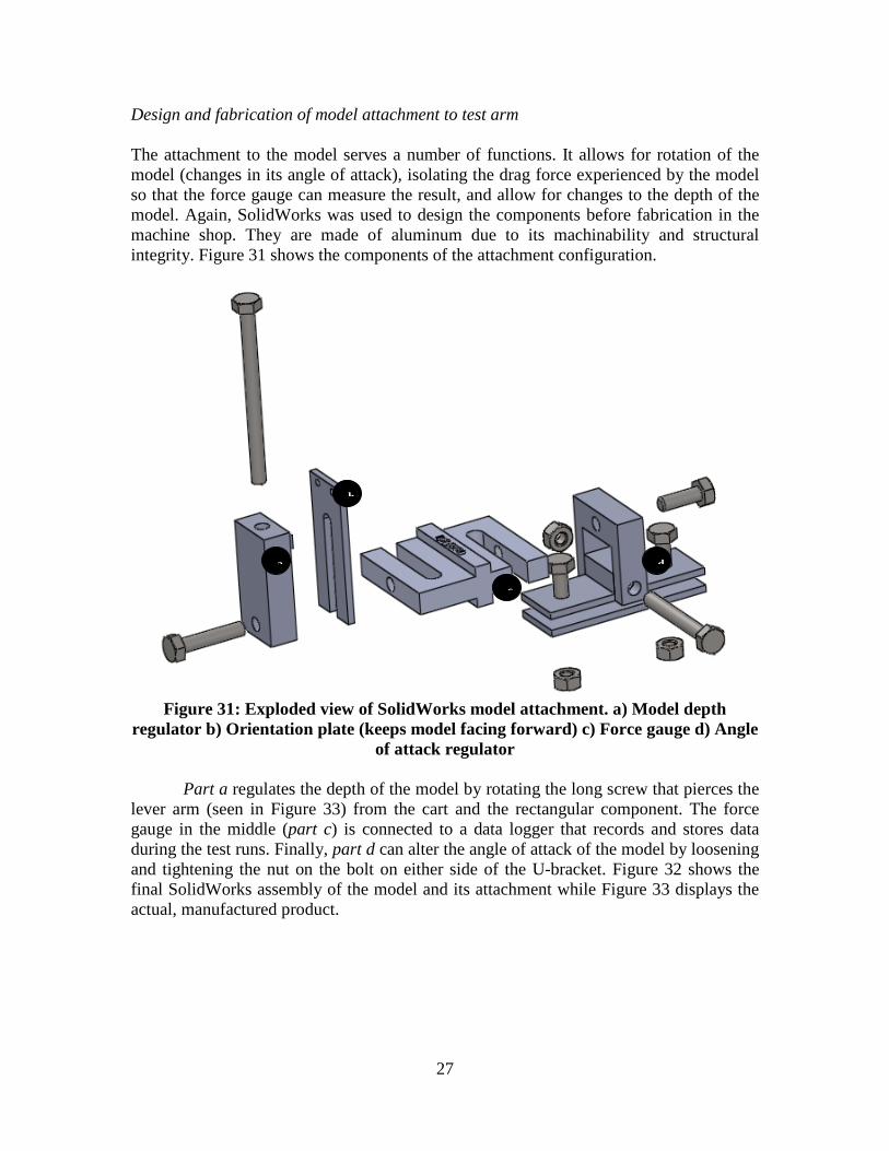
Design and fabrication of model attachment to test arm The attachment to the model serves a number of functions. It allows for rotation of the model (changes in its angle of attack), isolating the drag force experienced by the model so that the force gauge can measure the result, and allow for changes to the depth of the model. Again, SolidWorks was used to design the components before fabrication in the machine shop. They are made of aluminum due to its machinability and structural integrity. Figure 31 shows the components of the attachment configuration.

Figure 31: Exploded view of SolidWorks model attachment. a) Model depth

regulator b) Orientation plate (keeps model facing forward) c) Force gauge d) Angle of attack regulator

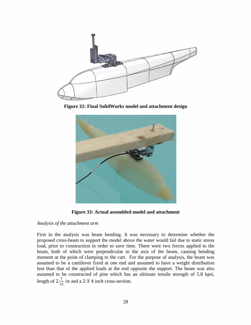
Part a regulates the depth of the model by rotating the long screw that pierces the lever arm (seen in Figure 33) from the cart and the rectangular component. The force gauge in the middle (part c) is connected to a data logger that records and stores data during the test runs. Finally, part d can alter the angle of attack of the model by loosening and tightening the nut on the bolt on either side of the U-bracket. Figure 32 shows the final SolidWorks assembly of the model and its attachment while Figure 33 displays the actual, manufactured product.

a

b

c

d

28

Figure 32: Final SolidWorks model and attachment design

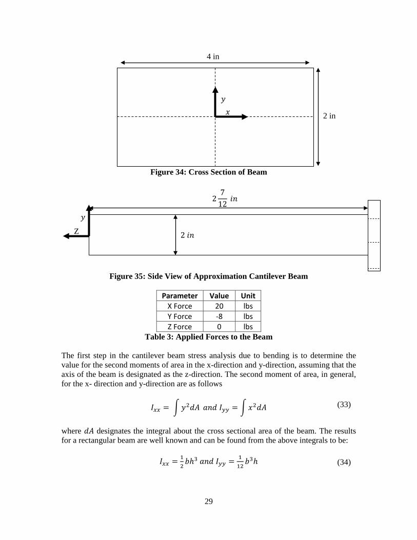
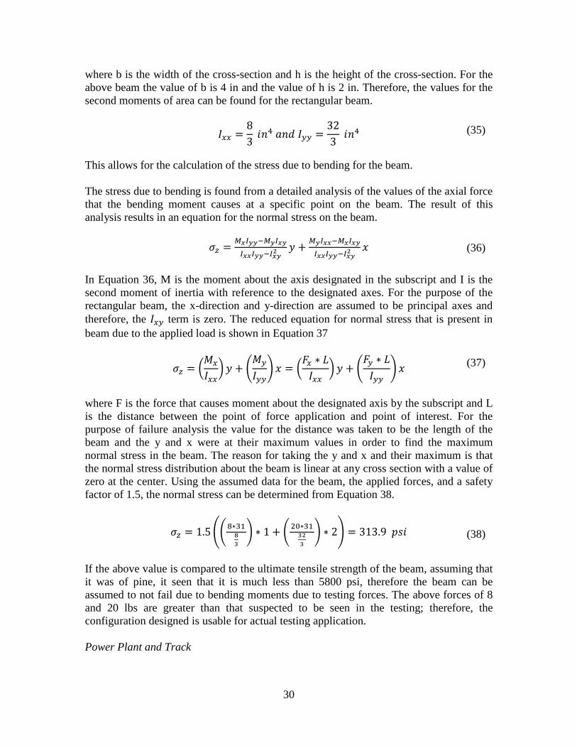
Figure 33: Actual assembled model and attachment Analysis of the attachment arm First in the analysis was beam bending. It was necessary to determine whether the proposed cross-beam to support the model above the water would fail due to static stress load, prior to construction in order to save time. There were two forces applied to the beam, both of which were perpendicular to the axis of the beam, causing bending moment at the point of clamping to the cart. For the purpose of analysis, the beam was assumed to be a cantilever fixed at one end and assumed to have a weight distribution less than that of the applied loads at the end opposite the support. The beam was also assumed to be constructed of pine which has an ultimate tensile strength of 5.8 kpsi, length of 2 7

12 𝑖𝑖 and a 2 𝑋 4 inch cross-section.

29

Figure 34: Cross Section of Beam

Figure 35: Side View of Approximation Cantilever Beam

Parameter Value Unit

X Force 20 lbs Y Force -8 lbs Z Force 0 lbs

Table 3: Applied Forces to the Beam The first step in the cantilever beam stress analysis due to bending is to determine the value for the second moments of area in the x-direction and y-direction, assuming that the axis of the beam is designated as the z-direction. The second moment of area, in general, for the x- direction and y-direction are as follows

𝐼𝑥𝑥 = �𝑦2𝑑𝐴 𝑎𝑖𝑑 𝐼𝑦𝑦 = �𝑥2𝑑𝐴

where 𝑑𝐴 designates the integral about the cross sectional area of the beam. The results for a rectangular beam are well known and can be found from the above integrals to be:

𝐼𝑥𝑥 = 12𝑏ℎ3 𝑎𝑖𝑑 𝐼𝑦𝑦 = 1

12𝑏3ℎ

4 in

2 in 𝑥 𝑦

𝑦

Z

27

12 𝑖𝑖

2 𝑖𝑖

(33)

(34)

30

where b is the width of the cross-section and h is the height of the cross-section. For the above beam the value of b is 4 in and the value of h is 2 in. Therefore, the values for the second moments of area can be found for the rectangular beam.

𝐼𝑥𝑥 =83

𝑖𝑖4 𝑎𝑖𝑑 𝐼𝑦𝑦 =323

𝑖𝑖4 This allows for the calculation of the stress due to bending for the beam. The stress due to bending is found from a detailed analysis of the values of the axial force that the bending moment causes at a specific point on the beam. The result of this analysis results in an equation for the normal stress on the beam.

𝜎𝑧 = 𝑀𝑥𝐼𝑦𝑦−𝑀𝑦𝐼𝑥𝑦𝐼𝑥𝑥𝐼𝑦𝑦−𝐼𝑥𝑦2

𝑦 + 𝑀𝑦𝐼𝑥𝑥−𝑀𝑥𝐼𝑥𝑦𝐼𝑥𝑥𝐼𝑦𝑦−𝐼𝑥𝑦2

𝑥

In Equation 36, M is the moment about the axis designated in the subscript and I is the second moment of inertia with reference to the designated axes. For the purpose of the rectangular beam, the x-direction and y-direction are assumed to be principal axes and therefore, the 𝐼𝑥𝑦 term is zero. The reduced equation for normal stress that is present in beam due to the applied load is shown in Equation 37

𝜎𝑧 = �𝑀𝑥

𝐼𝑥𝑥� 𝑦 + �

𝑀𝑦

𝐼𝑦𝑦� 𝑥 = �

𝐹𝑥 ∗ 𝐿𝐼𝑥𝑥

� 𝑦 + �𝐹𝑦 ∗ 𝐿𝐼𝑦𝑦

� 𝑥

where F is the force that causes moment about the designated axis by the subscript and L is the distance between the point of force application and point of interest. For the purpose of failure analysis the value for the distance was taken to be the length of the beam and the y and x were at their maximum values in order to find the maximum normal stress in the beam. The reason for taking the y and x and their maximum is that the normal stress distribution about the beam is linear at any cross section with a value of zero at the center. Using the assumed data for the beam, the applied forces, and a safety factor of 1.5, the normal stress can be determined from Equation 38.

𝜎𝑧 = 1.5��8∗3183� ∗ 1 + �20∗3132

3� ∗ 2� = 313.9 𝑝𝑠𝑖

If the above value is compared to the ultimate tensile strength of the beam, assuming that it was of pine, it seen that it is much less than 5800 psi, therefore the beam can be assumed to not fail due to bending moments due to testing forces. The above forces of 8 and 20 lbs are greater than that suspected to be seen in the testing; therefore, the configuration designed is usable for actual testing application. Power Plant and Track

(35)

(36)

(37)

(38)

31

The final part of the test design was to determine how it would be pulled and remain on a straight path. The power plant had to be able to pull the cart with the model attached to it at maximum speeds of 20 ft/s. The string needed to be able to hold the force of pulling the cart and the model. Finally, the two guiding strings needed to be strong and rigid enough to keep the cart on a straight path along the side of the pool.

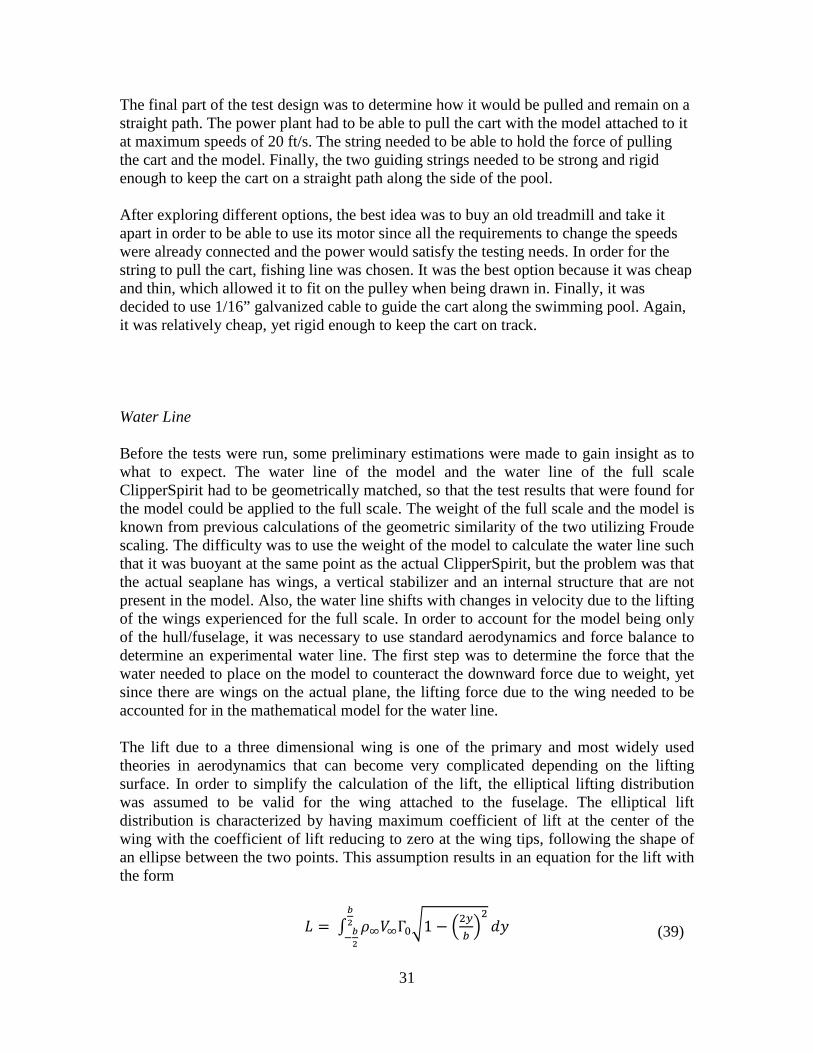
After exploring different options, the best idea was to buy an old treadmill and take it apart in order to be able to use its motor since all the requirements to change the speeds were already connected and the power would satisfy the testing needs. In order for the string to pull the cart, fishing line was chosen. It was the best option because it was cheap and thin, which allowed it to fit on the pulley when being drawn in. Finally, it was decided to use 1/16” galvanized cable to guide the cart along the swimming pool. Again, it was relatively cheap, yet rigid enough to keep the cart on track. Water Line Before the tests were run, some preliminary estimations were made to gain insight as to what to expect. The water line of the model and the water line of the full scale ClipperSpirit had to be geometrically matched, so that the test results that were found for the model could be applied to the full scale. The weight of the full scale and the model is known from previous calculations of the geometric similarity of the two utilizing Froude scaling. The difficulty was to use the weight of the model to calculate the water line such that it was buoyant at the same point as the actual ClipperSpirit, but the problem was that the actual seaplane has wings, a vertical stabilizer and an internal structure that are not present in the model. Also, the water line shifts with changes in velocity due to the lifting of the wings experienced for the full scale. In order to account for the model being only of the hull/fuselage, it was necessary to use standard aerodynamics and force balance to determine an experimental water line. The first step was to determine the force that the water needed to place on the model to counteract the downward force due to weight, yet since there are wings on the actual plane, the lifting force due to the wing needed to be accounted for in the mathematical model for the water line. The lift due to a three dimensional wing is one of the primary and most widely used theories in aerodynamics that can become very complicated depending on the lifting surface. In order to simplify the calculation of the lift, the elliptical lifting distribution was assumed to be valid for the wing attached to the fuselage. The elliptical lift distribution is characterized by having maximum coefficient of lift at the center of the wing with the coefficient of lift reducing to zero at the wing tips, following the shape of an ellipse between the two points. This assumption results in an equation for the lift with the form

𝐿 = ∫ 𝜌∞𝑉∞Γ0�1 − �2𝑦𝑏�2𝑑𝑦

𝑏2

−𝑏2 (39)

32

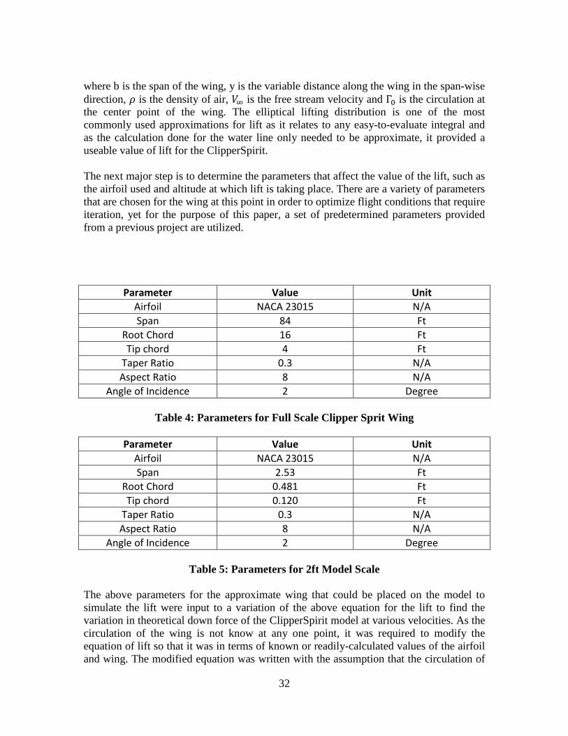
where b is the span of the wing, y is the variable distance along the wing in the span-wise direction, 𝜌 is the density of air, 𝑉∞ is the free stream velocity and Γ0 is the circulation at the center point of the wing. The elliptical lifting distribution is one of the most commonly used approximations for lift as it relates to any easy-to-evaluate integral and as the calculation done for the water line only needed to be approximate, it provided a useable value of lift for the ClipperSpirit. The next major step is to determine the parameters that affect the value of the lift, such as the airfoil used and altitude at which lift is taking place. There are a variety of parameters that are chosen for the wing at this point in order to optimize flight conditions that require iteration, yet for the purpose of this paper, a set of predetermined parameters provided from a previous project are utilized.

Parameter Value Unit Airfoil NACA 23015 N/A Span 84 Ft

Root Chord 16 Ft Tip chord 4 Ft

Taper Ratio 0.3 N/A Aspect Ratio 8 N/A

Angle of Incidence 2 Degree

Table 4: Parameters for Full Scale Clipper Sprit Wing

Parameter Value Unit Airfoil NACA 23015 N/A Span 2.53 Ft

Root Chord 0.481 Ft Tip chord 0.120 Ft

Taper Ratio 0.3 N/A Aspect Ratio 8 N/A

Angle of Incidence 2 Degree

Table 5: Parameters for 2ft Model Scale The above parameters for the approximate wing that could be placed on the model to simulate the lift were input to a variation of the above equation for the lift to find the variation in theoretical down force of the ClipperSpirit model at various velocities. As the circulation of the wing is not know at any one point, it was required to modify the equation of lift so that it was in terms of known or readily-calculated values of the airfoil and wing. The modified equation was written with the assumption that the circulation of

33

the wing was a function of the coefficient of lift and the chord length at that point, such that the equation for circulation was

Γ0 = 12𝑉∞𝑐𝐶𝑙

where c is the chord length and 𝐶𝑙 is the coefficient of lift for the airfoil at the specified angle of attack. Therefore, the modified lifting equation had the following form.

𝐿(𝛼) = 12𝜌∞𝑉∞2𝐶𝑙(𝛼)∫ �1 − �2𝑦

𝑏�2

(5.772 − 0.3|𝑦|𝑏2

−𝑏2) 𝑑𝑦

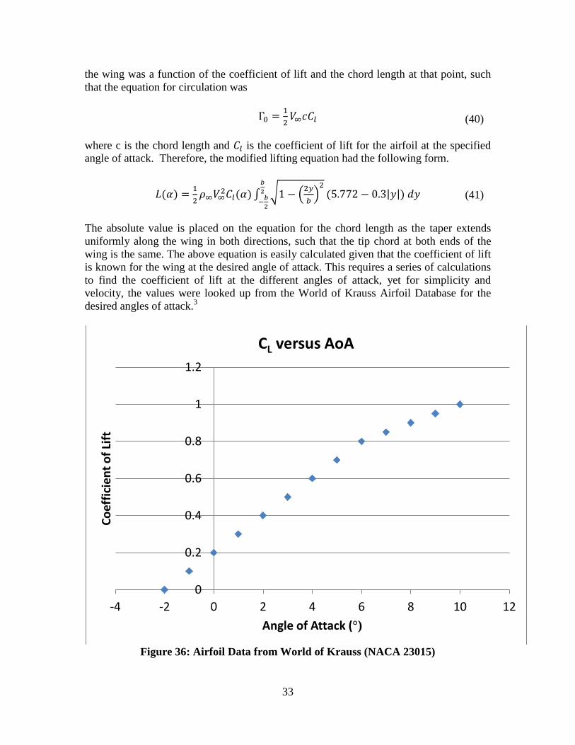
The absolute value is placed on the equation for the chord length as the taper extends uniformly along the wing in both directions, such that the tip chord at both ends of the wing is the same. The above equation is easily calculated given that the coefficient of lift is known for the wing at the desired angle of attack. This requires a series of calculations to find the coefficient of lift at the different angles of attack, yet for simplicity and velocity, the values were looked up from the World of Krauss Airfoil Database for the desired angles of attack.3

Figure 36: Airfoil Data from World of Krauss (NACA 23015)

0

0.2

0.4

0.6

0.8

1

1.2

-4 -2 0 2 4 6 8 10 12

Coef

ficie

nt o

f Lift

Angle of Attack (°)

CL versus AoA

(40)

(41)

34

Due to required testing parameters, the lift was needed to be calculated for angles varying from -2 to 10 degrees and for velocities varying from 0 to 24 feet per second. This requires a good deal of calculation, therefore a spreadsheet program was used to calculate the varied lift values for the different configurations. The next step after determining the lift that the wing places on the ClipperSpirit at different angles of attack and velocities is to determine the downward force the entire plane experiences. Due to the desired need of only a rough approximation of the water line, the only forces accounted for in the vertical direction were due to gravity and lift of the wing. The downward force was found by using the following simple relationship between the gravitational and lift force.

𝐷𝑜𝑤𝑖𝑤𝑎𝑟𝑑 𝐹𝑜𝑟𝑐𝑒 = 𝐹𝐷𝑜𝑤𝑛 = 𝑊𝑒𝑖𝑔ℎ𝑡 − 𝐿𝑖𝑓𝑡 = 𝑊𝑇𝑂 − 𝐿 The above is a self-explanatory, simplified relationship of the entire set of complex forces that may be present during operation of a seaplane at takeoff. For the above equation it was assumed that this was the force applied to the water in the vertical direction, therefore it is assumed that the water line was such that the buoyancy force the water applied to the model would be equal to this value. The buoyancy of water is a well known phenomenon in nature that has been determined to follow the mathematical relationship

𝐹 = 𝜌𝑤𝑎𝑡𝑒𝑟𝑉𝑤𝑎𝑡𝑒𝑟 where 𝜌𝑤𝑎𝑡𝑒𝑟 is the density of water and 𝑉𝑤𝑎𝑡𝑒𝑟 is the volume of water displaced. Using the fact that the density of water is 62.4 pounds per cubic foot, the required volume of displaced water was determined for each set of angle of attack and velocity. The final step to finding the water line was to define a method and determine an approximate shape for the volume that displaced the water. This is a difficult task as the actual shape of the bottom of the fuselage is based on a series of known cross-sections connected by lofts that create unknown mathematical shapes. This required the volume to be approximated by a known shape with a mathematical relationship that would result in a value for the distance above the step of the water line. The bottom of the fuselage was approximated as an irregular pyramid that has a known equation for the volume. This was the best shape for this approximation. The basic equation for the volume of a pyramid is

𝑉𝑝𝑦𝑟𝑎𝑚𝑖𝑑 = 13𝐵ℎ

where B is the area of the base and h is the height of the pyramid measured perpendicular to the base to the tip of the pyramid. The formula above is derived for the pyramid with an equilateral triangle base, yet is applicable to any triangular base as the area of the irregular triangle base could be redrawn as an equilateral triangle with the same area.

(42)

(43)

(44)

35

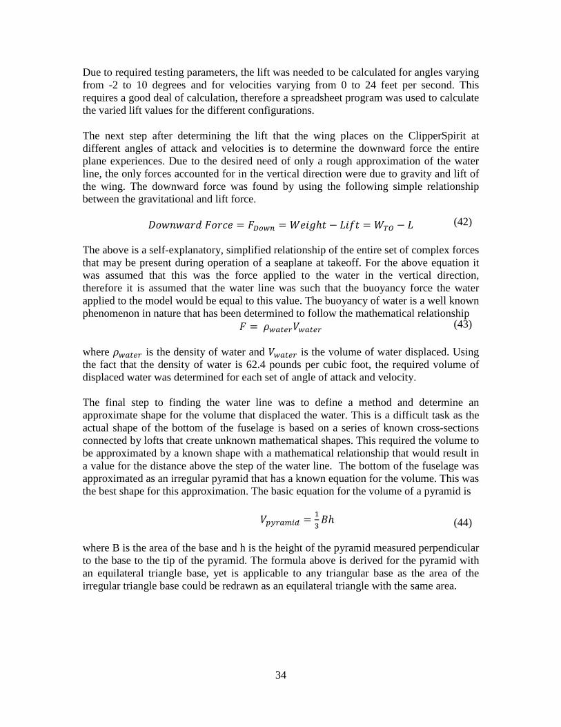
Figure 37: Approximation Shape for Volume of Displaced Water

The volume was designed so that it followed the equation

𝑉𝑤𝑎𝑡𝑒𝑟 = 13�12∗ 2ℎtan(70°) ℎ� �

ℎtan(𝜃)� + 1

3�12∗ 2ℎtan(70°) ℎ� �

ℎ∗𝑡𝑎𝑛(𝛼)tan (𝜃)

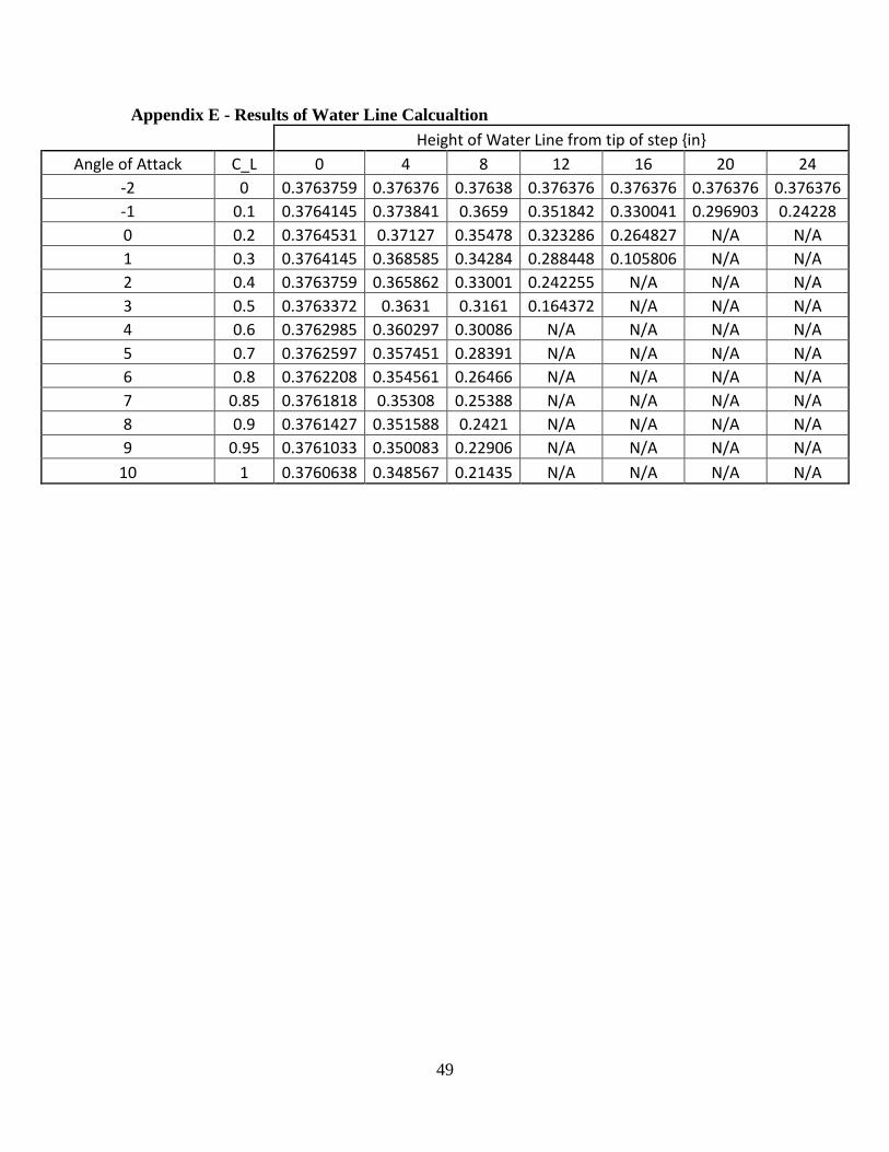
� where h was desired value for the water line height above the base of the step, 𝜃 is the angle of drop from the nose to the step locally and 𝛼 is the angle of attack. The above equation was derived from the basic equation for the volume of a pyramid and adapted to fit with the shape that the water sees from the base of the hull/fuselage. The second term in the equaion accounts for the fact that as the fuselage changes angle of attack, the shape that the water sees varies, therefore in order for the water line to always be meaured directly from the tip, the angle of attack term was added. The above equation was solved for h for each case of angle of attack and velocity combination and tabulated for testing application. Specific values were calculated for angles of attack from -2 to 15 in 1 degree increments and velocities of 0 to 24 in 4 ft/s increments. The general trend was that the deepest water line was approximately 0.376 above the tip of the step for all speeds at an angle of attack of -2° and that this decreased with increased speed and angle of attack.

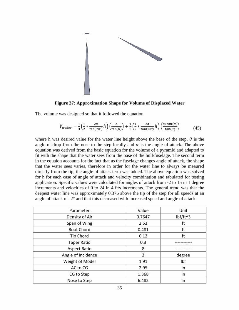
Parameter Value Unit Density of Air 0.7647 lbf/ft^3 Span of Wing 2.53 ft Root Chord 0.481 ft Tip Chord 0.12 ft

Taper Ratio 0.3 ------------ Aspect Ratio 8 -------------

Angle of Incidence 2 degree Weight of Model 1.91 lbf

AC to CG 2.95 in CG to Step 1.368 in

Nose to Step 6.482 in

(45)

36

Angle of Pyramid 1.01 degree Table 6: Values used in Cacluation of Water line

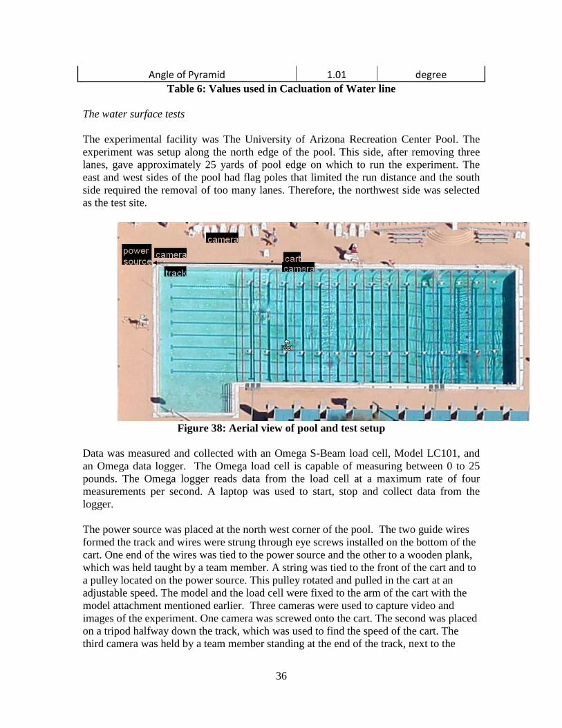
The water surface tests The experimental facility was The University of Arizona Recreation Center Pool. The experiment was setup along the north edge of the pool. This side, after removing three lanes, gave approximately 25 yards of pool edge on which to run the experiment. The east and west sides of the pool had flag poles that limited the run distance and the south side required the removal of too many lanes. Therefore, the northwest side was selected as the test site.

Figure 38: Aerial view of pool and test setup

Data was measured and collected with an Omega S-Beam load cell, Model LC101, and an Omega data logger. The Omega load cell is capable of measuring between 0 to 25 pounds. The Omega logger reads data from the load cell at a maximum rate of four measurements per second. A laptop was used to start, stop and collect data from the logger. The power source was placed at the north west corner of the pool. The two guide wires formed the track and wires were strung through eye screws installed on the bottom of the cart. One end of the wires was tied to the power source and the other to a wooden plank, which was held taught by a team member. A string was tied to the front of the cart and to a pulley located on the power source. This pulley rotated and pulled in the cart at an adjustable speed. The model and the load cell were fixed to the arm of the cart with the model attachment mentioned earlier. Three cameras were used to capture video and images of the experiment. One camera was screwed onto the cart. The second was placed on a tripod halfway down the track, which was used to find the speed of the cart. The third camera was held by a team member standing at the end of the track, next to the

37

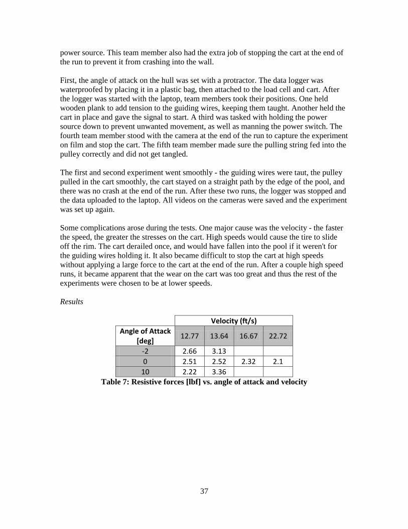
power source. This team member also had the extra job of stopping the cart at the end of the run to prevent it from crashing into the wall. First, the angle of attack on the hull was set with a protractor. The data logger was waterproofed by placing it in a plastic bag, then attached to the load cell and cart. After the logger was started with the laptop, team members took their positions. One held wooden plank to add tension to the guiding wires, keeping them taught. Another held the cart in place and gave the signal to start. A third was tasked with holding the power source down to prevent unwanted movement, as well as manning the power switch. The fourth team member stood with the camera at the end of the run to capture the experiment on film and stop the cart. The fifth team member made sure the pulling string fed into the pulley correctly and did not get tangled. The first and second experiment went smoothly - the guiding wires were taut, the pulley pulled in the cart smoothly, the cart stayed on a straight path by the edge of the pool, and there was no crash at the end of the run. After these two runs, the logger was stopped and the data uploaded to the laptop. All videos on the cameras were saved and the experiment was set up again. Some complications arose during the tests. One major cause was the velocity - the faster the speed, the greater the stresses on the cart. High speeds would cause the tire to slide off the rim. The cart derailed once, and would have fallen into the pool if it weren't for the guiding wires holding it. It also became difficult to stop the cart at high speeds without applying a large force to the cart at the end of the run. After a couple high speed runs, it became apparent that the wear on the cart was too great and thus the rest of the experiments were chosen to be at lower speeds. Results

Velocity (ft/s) Angle of Attack

[deg] 12.77 13.64 16.67 22.72

-2 2.66 3.13 0 2.51 2.52 2.32 2.1

10 2.22 3.36 Table 7: Resistive forces [lbf] vs. angle of attack and velocity

38

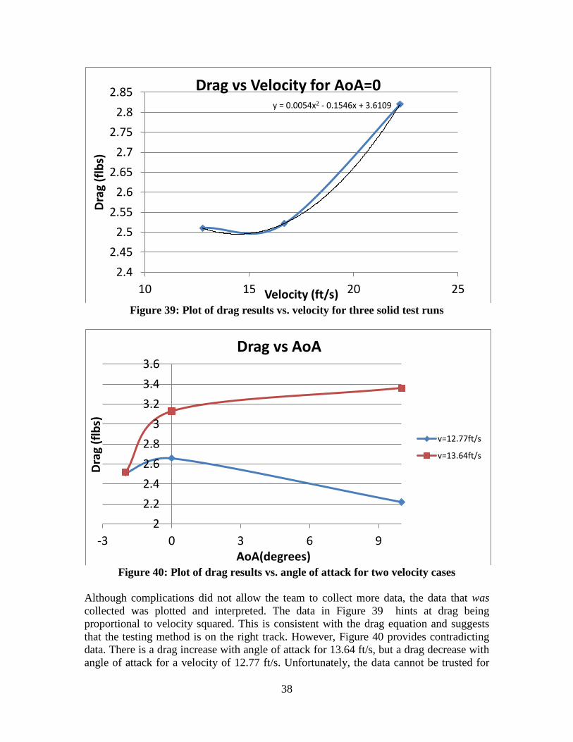
Figure 39: Plot of drag results vs. velocity for three solid test runs

Figure 40: Plot of drag results vs. angle of attack for two velocity cases

Although complications did not allow the team to collect more data, the data that was collected was plotted and interpreted. The data in Figure 39 hints at drag being proportional to velocity squared. This is consistent with the drag equation and suggests that the testing method is on the right track. However, Figure 40 provides contradicting data. There is a drag increase with angle of attack for 13.64 ft/s, but a drag decrease with angle of attack for a velocity of 12.77 ft/s. Unfortunately, the data cannot be trusted for

y = 0.0054x2 - 0.1546x + 3.6109

2.42.45

2.52.55

2.62.65

2.72.75

2.82.85

10 15 20 25

Dra

g (fl

bs)

Velocity (ft/s)

Drag vs Velocity for AoA=0

22.22.42.62.8

33.23.43.6

-3 0 3 6 9

Drag

(flb

s)

AoA(degrees)

Drag vs AoA

v=12.77ft/s

v=13.64ft/s

39

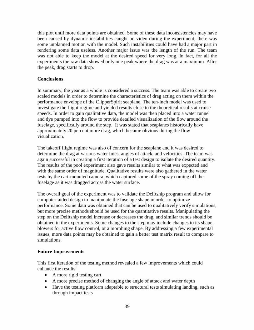
this plot until more data points are obtained. Some of these data inconsistencies may have been caused by dynamic instabilities caught on video during the experiment; there was some unplanned motion with the model. Such instabilities could have had a major part in rendering some data useless. Another major issue was the length of the run. The team was not able to keep the model at the desired speed for very long. In fact, for all the experiments the raw data showed only one peak where the drag was at a maximum. After the peak, drag starts to drop. Conclusions In summary, the year as a whole is considered a success. The team was able to create two scaled models in order to determine the characteristics of drag acting on them within the performance envelope of the ClipperSpirit seaplane. The ten-inch model was used to investigate the flight regime and yielded results close to the theoretical results at cruise speeds. In order to gain qualitative data, the model was then placed into a water tunnel and dye pumped into the flow to provide detailed visualization of the flow around the fuselage, specifically around the step. It was stated that seaplanes historically have approximately 20 percent more drag, which became obvious during the flow visualization. The takeoff flight regime was also of concern for the seaplane and it was desired to determine the drag at various water lines, angles of attack, and velocities. The team was again successful in creating a first iteration of a test design to isolate the desired quantity. The results of the pool experiment also gave results similar to what was expected and with the same order of magnitude. Qualitative results were also gathered in the water tests by the cart-mounted camera, which captured some of the spray coming off the fuselage as it was dragged across the water surface. The overall goal of the experiment was to validate the Delftship program and allow for computer-aided design to manipulate the fuselage shape in order to optimize performance. Some data was obtained that can be used to qualitatively verify simulations, but more precise methods should be used for the quantitative results. Manipulating the step on the Delftship model increase or decreases the drag, and similar trends should be obtained in the experiments. Some changes to the step may include changes to its shape, blowers for active flow control, or a morphing shape. By addressing a few experimental issues, more data points may be obtained to gain a better test matrix result to compare to simulations. Future Improvements This first iteration of the testing method revealed a few improvements which could enhance the results:

• A more rigid testing cart • A more precise method of changing the angle of attack and water depth • Have the testing platform adaptable to structural tests simulating landing, such as

through impact tests

40

References [1] "Experimental Methods in Marine Hydrodynamics." Web. 1 Nov. 2011.

<http://www.ivt.ntnu.no/imt/courses/tmr7/lecture/Scaling_Laws.pdf>. [2] Korotkin, Alexander I. Added Mass of Ship Structures. 1st ed. Springer, 2008. Print. [3] "NACA 23015." Airfoil Investigation Database. University of Illinois at Urbana-

Champaign Airfoil Coordinates Database, 25 Feb. 2012. Web. 15 Apr. 2012. <http://www.worldofkrauss.com/foils/1701>.

[4] Nicolai, Leland M., Grant Carichner, and Leland M. Nicolai. Fundamentals of

Aircraft and Airship Design. Vol. 1. Reston, VA: American Institute of Aeronautics and Astronautics, 2010. Print.

[5] "Part 25 - AIRWORTHINESS STANDARDS: TRANSPORT CATEGORY

AIRPLANES." Federal Aviation Regulations. Web. Fall 2001. [6] Techet, A. H. "Hydrodynamics." MIT Open Courseware. MIT, 30 Aug. 2005. Web.

Fall 2011. <http://ocw.mit.edu/courses/mechanical-engineering/2-016-hydrodynamics-13-012-fall-2005/readings/2005reading6.pdf>.

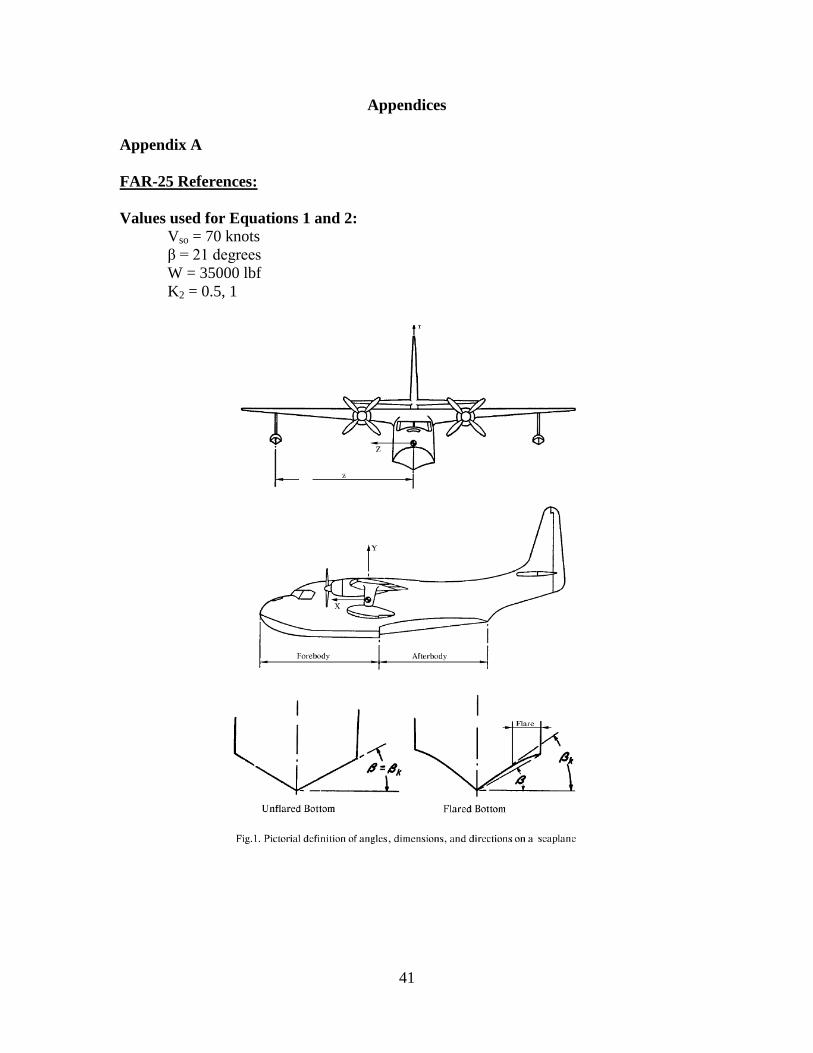
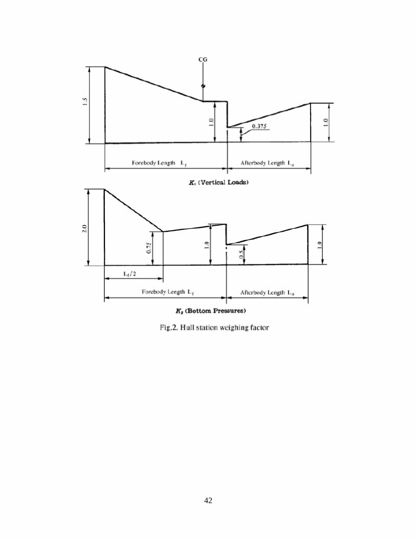
41

Appendices Appendix A FAR-25 References: Values used for Equations 1 and 2: Vso = 70 knots β = 21 degrees W = 35000 lbf K2 = 0.5, 1

42

43

Wind Tunnel Mount

44

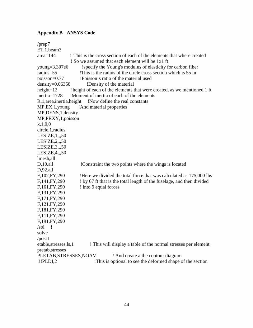
Appendix B - ANSYS Code /prep7 ET,1,beam3 area=144 ! This is the cross section of each of the elements that where created ! So we assumed that each element will be 1x1 ft young=3.307e6 !specify the Young's modulus of elasticity for carbon fiber radius=55 !This is the radius of the circle cross section which is 55 in poisson=0.77 !Poisson’s ratio of the material used density=0.06358 !Density of the material height=12 !height of each of the elements that were created, as we mentioned 1 ft inertia=1728 !Moment of inertia of each of the elements R,1,area,inertia,height !Now define the real constants MP,EX,1,young !And material properties MP,DENS,1,density MP,PRXY,1,poisson k,1,0,0 circle,1,radius LESIZE,1,,,50 LESIZE,2,,,50 LESIZE,3,,,50 LESIZE,4,,,50 lmesh,all D,10,all !Constraint the two points where the wings is located D,92,all F,102,FY,290 !Here we divided the total force that was calculated as 175,000 lbs F,141,FY,290 ! by 67 ft that is the total length of the fuselage, and then divided F,161,FY,290 ! into 9 equal forces F,131,FY,290 F,171,FY,290 F,121,FY,290 F,181,FY,290 F,111,FY,290 F,191,FY,290 /sol ! solve /post1 etable,stresses,ls,1 ! This will display a table of the normal stresses per element pretab,stresses PLETAB,STRESSES,NOAV ! And create a the contour diagram !!!PLDI,2 !This is optional to see the deformed shape of the section

45

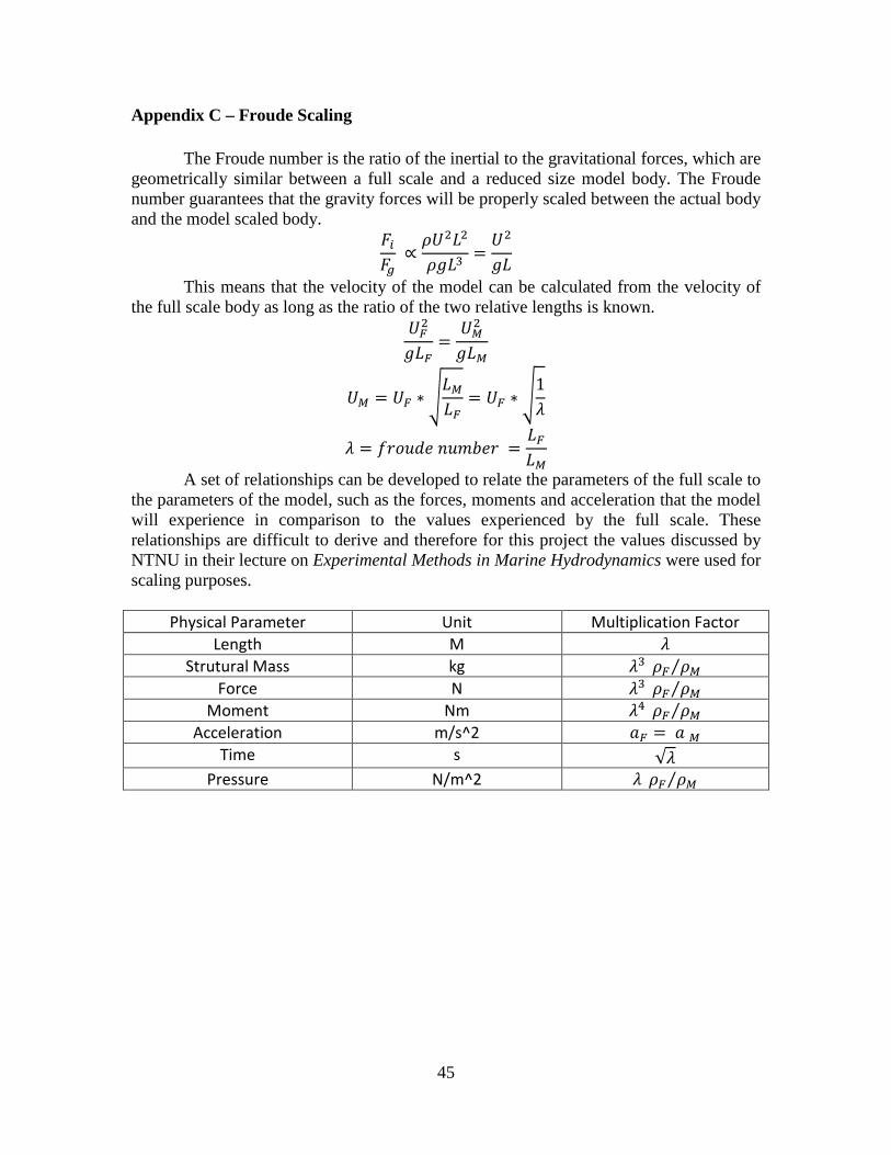
Appendix C – Froude Scaling The Froude number is the ratio of the inertial to the gravitational forces, which are geometrically similar between a full scale and a reduced size model body. The Froude number guarantees that the gravity forces will be properly scaled between the actual body and the model scaled body.

𝐹𝑖𝐹𝑔

∝𝜌𝑈2𝐿2

𝜌𝑔𝐿3=𝑈2

𝑔𝐿

This means that the velocity of the model can be calculated from the velocity of the full scale body as long as the ratio of the two relative lengths is known.

𝑈𝐹2

𝑔𝐿𝐹=

𝑈𝑀2

𝑔𝐿𝑀

𝑈𝑀 = 𝑈𝐹 ∗ �𝐿𝑀𝐿𝐹

= 𝑈𝐹 ∗ �1𝜆

𝜆 = 𝑓𝑟𝑜𝑢𝑑𝑒 𝑖𝑢𝑚𝑏𝑒𝑟 =𝐿𝐹𝐿𝑀

A set of relationships can be developed to relate the parameters of the full scale to the parameters of the model, such as the forces, moments and acceleration that the model will experience in comparison to the values experienced by the full scale. These relationships are difficult to derive and therefore for this project the values discussed by NTNU in their lecture on Experimental Methods in Marine Hydrodynamics were used for scaling purposes.

Physical Parameter Unit Multiplication Factor Length M 𝜆

Strutural Mass kg 𝜆3 𝜌𝐹 𝜌𝑀⁄ Force N 𝜆3 𝜌𝐹 𝜌𝑀⁄

Moment Nm 𝜆4 𝜌𝐹 𝜌𝑀⁄ Acceleration m/s^2 𝑎𝐹 = 𝑎 𝑀

Time s √𝜆 Pressure N/m^2 𝜆 𝜌𝐹 𝜌𝑀⁄

46

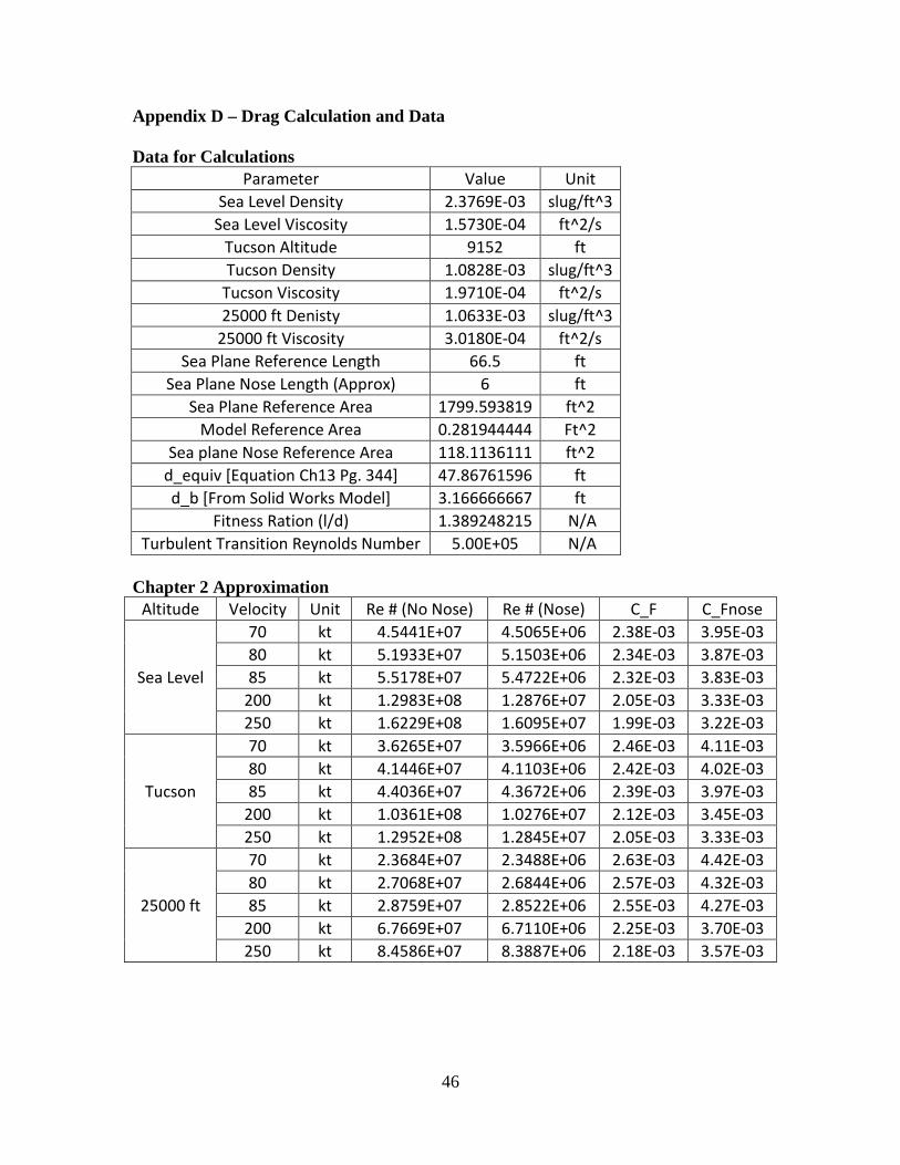
Appendix D – Drag Calculation and Data Data for Calculations

Parameter Value Unit Sea Level Density 2.3769E-03 slug/ft^3

Sea Level Viscosity 1.5730E-04 ft^2/s Tucson Altitude 9152 ft Tucson Density 1.0828E-03 slug/ft^3

Tucson Viscosity 1.9710E-04 ft^2/s 25000 ft Denisty 1.0633E-03 slug/ft^3

25000 ft Viscosity 3.0180E-04 ft^2/s Sea Plane Reference Length 66.5 ft

Sea Plane Nose Length (Approx) 6 ft Sea Plane Reference Area 1799.593819 ft^2

Model Reference Area 0.281944444 Ft^2 Sea plane Nose Reference Area 118.1136111 ft^2

d_equiv [Equation Ch13 Pg. 344] 47.86761596 ft d_b [From Solid Works Model] 3.166666667 ft

Fitness Ration (l/d) 1.389248215 N/A Turbulent Transition Reynolds Number 5.00E+05 N/A

Chapter 2 Approximation

Altitude Velocity Unit Re # (No Nose) Re # (Nose) C_F C_Fnose

Sea Level

70 kt 4.5441E+07 4.5065E+06 2.38E-03 3.95E-03 80 kt 5.1933E+07 5.1503E+06 2.34E-03 3.87E-03 85 kt 5.5178E+07 5.4722E+06 2.32E-03 3.83E-03

200 kt 1.2983E+08 1.2876E+07 2.05E-03 3.33E-03 250 kt 1.6229E+08 1.6095E+07 1.99E-03 3.22E-03

Tucson

70 kt 3.6265E+07 3.5966E+06 2.46E-03 4.11E-03 80 kt 4.1446E+07 4.1103E+06 2.42E-03 4.02E-03 85 kt 4.4036E+07 4.3672E+06 2.39E-03 3.97E-03

200 kt 1.0361E+08 1.0276E+07 2.12E-03 3.45E-03 250 kt 1.2952E+08 1.2845E+07 2.05E-03 3.33E-03

25000 ft

70 kt 2.3684E+07 2.3488E+06 2.63E-03 4.42E-03 80 kt 2.7068E+07 2.6844E+06 2.57E-03 4.32E-03 85 kt 2.8759E+07 2.8522E+06 2.55E-03 4.27E-03

200 kt 6.7669E+07 6.7110E+06 2.25E-03 3.70E-03 250 kt 8.4586E+07 8.3887E+06 2.18E-03 3.57E-03

47

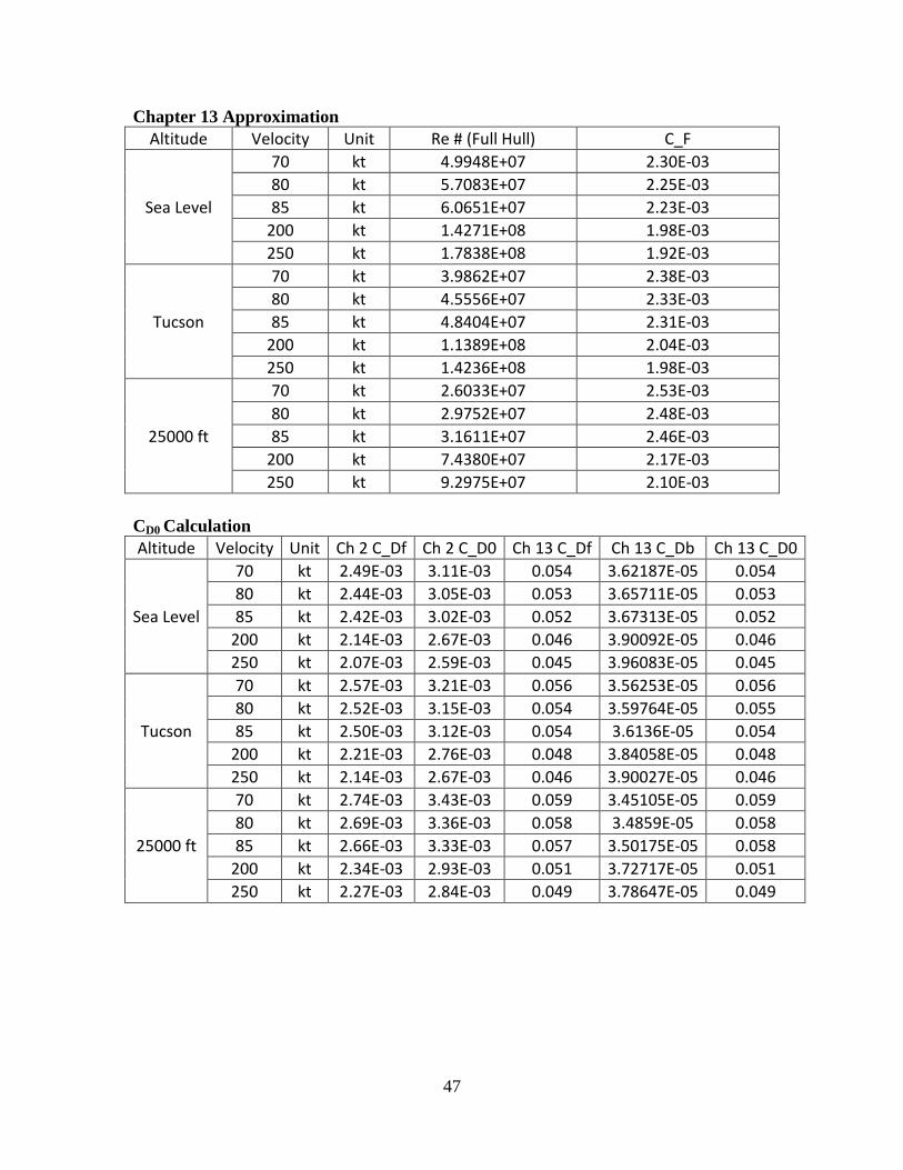
Chapter 13 Approximation Altitude Velocity Unit Re # (Full Hull) C_F

Sea Level

70 kt 4.9948E+07 2.30E-03 80 kt 5.7083E+07 2.25E-03 85 kt 6.0651E+07 2.23E-03

200 kt 1.4271E+08 1.98E-03 250 kt 1.7838E+08 1.92E-03

Tucson

70 kt 3.9862E+07 2.38E-03 80 kt 4.5556E+07 2.33E-03 85 kt 4.8404E+07 2.31E-03

200 kt 1.1389E+08 2.04E-03 250 kt 1.4236E+08 1.98E-03

25000 ft

70 kt 2.6033E+07 2.53E-03 80 kt 2.9752E+07 2.48E-03 85 kt 3.1611E+07 2.46E-03

200 kt 7.4380E+07 2.17E-03 250 kt 9.2975E+07 2.10E-03

CD0 Calculation Altitude Velocity Unit Ch 2 C_Df Ch 2 C_D0 Ch 13 C_Df Ch 13 C_Db Ch 13 C_D0

Sea Level

70 kt 2.49E-03 3.11E-03 0.054 3.62187E-05 0.054 80 kt 2.44E-03 3.05E-03 0.053 3.65711E-05 0.053 85 kt 2.42E-03 3.02E-03 0.052 3.67313E-05 0.052

200 kt 2.14E-03 2.67E-03 0.046 3.90092E-05 0.046 250 kt 2.07E-03 2.59E-03 0.045 3.96083E-05 0.045

Tucson

70 kt 2.57E-03 3.21E-03 0.056 3.56253E-05 0.056 80 kt 2.52E-03 3.15E-03 0.054 3.59764E-05 0.055 85 kt 2.50E-03 3.12E-03 0.054 3.6136E-05 0.054

200 kt 2.21E-03 2.76E-03 0.048 3.84058E-05 0.048 250 kt 2.14E-03 2.67E-03 0.046 3.90027E-05 0.046

25000 ft

70 kt 2.74E-03 3.43E-03 0.059 3.45105E-05 0.059 80 kt 2.69E-03 3.36E-03 0.058 3.4859E-05 0.058 85 kt 2.66E-03 3.33E-03 0.057 3.50175E-05 0.058

200 kt 2.34E-03 2.93E-03 0.051 3.72717E-05 0.051 250 kt 2.27E-03 2.84E-03 0.049 3.78647E-05 0.049

48

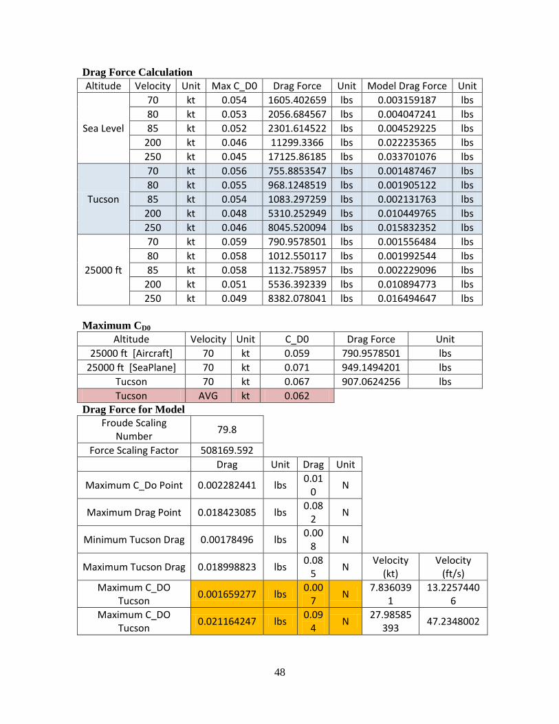
Drag Force Calculation Altitude Velocity Unit Max C_D0 Drag Force Unit Model Drag Force Unit

Sea Level

70 kt 0.054 1605.402659 lbs 0.003159187 lbs 80 kt 0.053 2056.684567 lbs 0.004047241 lbs 85 kt 0.052 2301.614522 lbs 0.004529225 lbs

200 kt 0.046 11299.3366 lbs 0.022235365 lbs 250 kt 0.045 17125.86185 lbs 0.033701076 lbs

Tucson

70 kt 0.056 755.8853547 lbs 0.001487467 lbs 80 kt 0.055 968.1248519 lbs 0.001905122 lbs 85 kt 0.054 1083.297259 lbs 0.002131763 lbs

200 kt 0.048 5310.252949 lbs 0.010449765 lbs 250 kt 0.046 8045.520094 lbs 0.015832352 lbs

25000 ft

70 kt 0.059 790.9578501 lbs 0.001556484 lbs 80 kt 0.058 1012.550117 lbs 0.001992544 lbs 85 kt 0.058 1132.758957 lbs 0.002229096 lbs

200 kt 0.051 5536.392339 lbs 0.010894773 lbs 250 kt 0.049 8382.078041 lbs 0.016494647 lbs

Maximum CD0

Altitude Velocity Unit C_D0 Drag Force Unit 25000 ft [Aircraft] 70 kt 0.059 790.9578501 lbs

25000 ft [SeaPlane] 70 kt 0.071 949.1494201 lbs Tucson 70 kt 0.067 907.0624256 lbs Tucson AVG kt 0.062

Drag Force for Model Froude Scaling

Number 79.8

Force Scaling Factor 508169.592 Drag Unit Drag Unit

Maximum C_Do Point 0.002282441 lbs 0.01

0 N

Maximum Drag Point 0.018423085 lbs 0.08

2 N

Minimum Tucson Drag 0.00178496 lbs 0.00

8 N

Maximum Tucson Drag 0.018998823 lbs 0.08

5 N

Velocity (kt)

Velocity (ft/s)

Maximum C_DO Tucson

0.001659277 lbs 0.00

7 N

7.8360391

13.22574406

Maximum C_DO Tucson

0.021164247 lbs 0.09

4 N

27.98585393

47.2348002

49

Appendix E - Results of Water Line Calcualtion

Height of Water Line from tip of step {in}

Angle of Attack C_L 0 4 8 12 16 20 24 -2 0 0.3763759 0.376376 0.37638 0.376376 0.376376 0.376376 0.376376 -1 0.1 0.3764145 0.373841 0.3659 0.351842 0.330041 0.296903 0.24228 0 0.2 0.3764531 0.37127 0.35478 0.323286 0.264827 N/A N/A 1 0.3 0.3764145 0.368585 0.34284 0.288448 0.105806 N/A N/A 2 0.4 0.3763759 0.365862 0.33001 0.242255 N/A N/A N/A 3 0.5 0.3763372 0.3631 0.3161 0.164372 N/A N/A N/A 4 0.6 0.3762985 0.360297 0.30086 N/A N/A N/A N/A 5 0.7 0.3762597 0.357451 0.28391 N/A N/A N/A N/A 6 0.8 0.3762208 0.354561 0.26466 N/A N/A N/A N/A 7 0.85 0.3761818 0.35308 0.25388 N/A N/A N/A N/A 8 0.9 0.3761427 0.351588 0.2421 N/A N/A N/A N/A 9 0.95 0.3761033 0.350083 0.22906 N/A N/A N/A N/A

10 1 0.3760638 0.348567 0.21435 N/A N/A N/A N/A