A6523 Signal Modeling, Statistical Inference and

Data Mining in Astrophysics

Spring 2015 http://www.astro.cornell.edu/~cordes/A6523

Lecture 25:!–  Markov Processes and Markov Chain Monte Carlo!

!•  Chapter 29 of Mackay (Monte Carlo Methods) !

http://www.inference.phy.cam.ac.uk/mackay/itila/!•  Chapter 12 in Gregory (MCMC)!•  An Introduction to MCMC for Machine Learning

(Andrieu et al. 2003, Machine Learning, 50, 5!•  Genetic Algorithms: Principles of Natural Selection

Applied to Computation (Stephanie Forrest, Science 1993, 261, 872) !

!!

!

Markov Processes

•  Markov processes are used for modeling as well as in statistical inference problems.!

•  Markov processes are generally nth order: !– The current state of a system may depend on n

previous states!– Most applications consider 1st order processes!

•  Hidden Markov processes: !– A physical system may involve transitions

between discrete states, but observables my reflect those states only indirectly (e.g. measurement noise, other physics, etc.) !

Markov Chains and Markov Processes

Definitions: A Markov process has future samples determined only by the present state andby a transition probability from the present state to a future state. A Markov chain is one thathas a countable number of states.

Transitions between states are described by an n ⇥ n stochastic matrix Q with elements qijcomprising the probabilities for changing in a single time step from state si to state sj with i, j =1, . . . , n. The state probability vector P has elements comprising the ensemble probability offinding the system in each state.

E.g. for a three-state system:

States = {s1, s2, · · · , sn}, Q =

�

⇤q11 q12 q13q21 q22 q23q31 q32 q33

⇥

⌅ .

Normalization across a row is⇧

j qij = 1 since the system must be in some state at any time.In a single time step the probability for staying in the ith state is the “metastability” qii and theprobability for residing in that state for a time T is proportional to qTii .

1

Example of a two-state Markov process

States = {s1, s2}, Q =

✓q11 q12

q21 q22

◆.

So

Q

2 =

✓q11 q12

q21 q22

◆✓q11 q12

q21 q22

◆=

✓q

211 + q12q21 q11q12 + q12q22

q21q11 + q22q21 q21q12 + q

222

◆

We want limt!1Q

t.

This gets messy very quickly even though there are only two independent quantitis, since q12 =1 � q11 and q21 = 1 � q22.

But it can be shown that

Q

1 =

✓p1 p2

p1 p2

◆where p1 =

T1

T1 + T2p2 =

T2

T1 + T2

andT1 = (1 � q11)

�1 and T2 = (1 � q22)�1

.

Thus the transition probabilities q11, q22 determine both the mean lifetime of each state T1 andT2 and the probabilities p1 and p2 of finding the process in each state.

5

Two-state Markov Processes

The probability density function (PDF) for the duration of a given state is therefore a geometricseries that sums to

fT (T ) = T�1i

�1� T�1

i

⇥T�1, T = 1, 2, · · · , (1)

with mean and rms values

Ti = (1� qii)�1, �Ti/Ti =

⇧qii. (2)

Asymptotic behavior as the number of steps ⇤ ⌅:

The transition matrix after t steps is Qt. Under the reasonable assumptions that all elements ofQ are non-negative and that all states are accessible in a finite number of steps, Qt converges toa steady-state form Q⌅ as t ⇤ ⌅ that has identical rows. Each row of Q⌅ is equal to the stateprobability vector P , the elements of which are the probabilities that a given time sample is ina particular state. P also equals the normalized left eigenvector of Q that has unity eigenvalue,i.e. PQ = P (e.g. Papoulis). For P to exist, the determinant det(Q � I) = 0 (where Iis the identity matrix), but this is automatically satisfied for a stochastic matrix correspondingto a stationary process. Convergence of Qt to a matrix with identical rows implies that thetransition probabilities trend to those appropriate for an i.i.d. process when the time step t ismuch larger than the mean lifetimes Ti of any of the states. For a two-state system P haselements p1 = (1� q22)/(2� q11 � q22) and p2 = 1� P1.

2

Utility of Markov processes:

1. Modeling: Many processes in the lab and in nature are consistent with being Markovchains. The key elements are a set of discrete states and transitions that are random but areaccording to a transition matrix.

2. Sampling: A Markov chain can define a trajectory in the relevant space which can be usedto randomly but efficiently sample the space. The key aspect of Markov Chain Monte Carlois that the trajectory conforms statistically to the asymptotic form of the transition matrix.

3

First order Markov processes: exponential PDFs for state durations

Pure two-state processes with different transition probabilities

Two-states with a periodic driving function à quasi-periodic state switching

State Changes in Pulsars B1931+24  

Kramer et al. 2006

13 yr of state changes (Young et al. 2013)

State durations are widely but NOT exponentially distributed

Stochastic resonance model can produce similar histograms

A strictly periodic forcing function (e.g. orbit) can produce quasi-periodic state changes

Statistics are nice but what are the physics? Effective potential of a two state system

State changes = stochastic jumps between wells

Stochastic resonance is from periodic modulation of the potential

A pulsar magnetosphere + accelerator is essentially a diode circuit with a return current

Markov switching and stochastic resonance are seen in laboratory diode circuits Pulsars more complicated because they are 2D circuits Periodic forcing in the equatorial disk can drive SR

Recent models (Liu, Spitkovsky, Timokhin, +) incorporate disks for the return current

Identifying Metastable States of Folding ProteinsAbhinav Jain and Gerhard Stock*

Biomolecular Dynamics, Institute of Physics, Albert Ludwigs University, 79104 Freiburg, Germany

*S Supporting Information

ABSTRACT: Recent molecular dynamics simulations of biopolymers have shown that in many cases the global features of thefree energy landscape can be characterized in terms of the metastable conformational states of the system. To identify thesestates, a conceptionally and computationally simple approach is proposed. It consists of (i) an initial preprocessing via principalcomponent analysis to reduce the dimensionality of the data, followed by k-means clustering to generate up to 104 microstates,(ii) the most probable path algorithm to identify the metastable states of the system, and (iii) boundary corrections of these statesvia the introduction of cluster cores in order to obtain the correct dynamics. By adopting two well-studied model problems,hepta-alanine and the villin headpiece protein, the potential and the performance of the approach are demonstrated.

1. INTRODUCTIONWhile molecular dynamics (MD) simulations account for thestructure and dynamics of biomolecules in microscopic detail,they generate huge amounts of data. To extract the essentialinformation and reduce the complex and highly correlatedbiomolecular motion from 3N atomic coordinates to a fewcollective degrees of freedom, dimensionality reductionmethods such as principal component analysis (PCA) arecommonly employed.1−5 The resulting low-dimensionalrepresentation of the dynamics can then be used to constructthe free energy landscape ΔG(V) = −kBT ln P(V), where P isthe probability distribution of the molecular system along theprincipal components V = {V1,V2,...}. Characterized by itsminima (which represent the metastable conformational statesof the systems) and its barriers (which connect these states),the energy landscape allows us to account for the pathways andtheir kinetics occurring in a biomolecular process.6−8

Recent simulations of peptides, proteins, and RNA haveshown that in many cases the free energy landscape can be wellcharacterized in terms of metastable conformational states.9−12

As an example, Figure 1A shows a two-dimensional free energylandscape of hepta-alanine13 (Ala7) obtained from an 800 nsMD simulation with subsequent PCA of the ϕ, ψ backbonedihedral angles (see section 3). The purple circles on thecontour plot readily indicate about 30 well-defined minima (orbasins) of the energy surface. They correspond to metastableconformational states, which can be employed to construct atransition network of the dynamics of the system.9−27 Thenetwork can be analyzed to reveal the relevant pathways of theconsidered process, or to discuss general features of the systemsuch as the topology (i.e., a hierarchical structure) of the energylandscape and network properties such as scale-freeness. Also,in protein folding, metastable states have emerged as a newparadigm.9,11 Augmenting the funnel picture of folding, thepresence of thermally populated metastable states may result inan ensemble of (rather than one or a few) folding pathways.19

Moreover, they can result in kinetic traps, which mayconsiderably extend the average folding time. As an example,Figure 1B shows the free energy landscape of the villinheadpiece subdomain,28−37 obtained from a PCA of extensive

folding trajectories by Pande and co-workers33 (see section 4).Due to the high dimensionality of the energy landscape, thetwo-dimensional projection only vaguely indicates the multipleminima of the protein.Although energy landscapes as in Figure 1 appear to easily

provide the location of the energy minima, in general it turnsout that metastable states are surprisingly difficult to identify,even for a seemingly simple system like Ala7. To partition theconformational space into clusters of data points representingthe states, one may use either geometric clustering methodssuch as k-means,38 which require only data in a metric space, orkinetic clustering methods, which additionally require dynam-ical information on the process.9−27 While geometrical methodsare fast and easy to use, they show several well-known flaws.For example, since they usually require one to fix the number ofclusters k beforehand, it easily happens that one combines twoseparate states into one (if k is chosen too small) or cuts onestate into two (if k is chosen too large). Another problem is theappropriate definition of the border between two clusters. Froma dynamical point of view, the correct border is clearly locatedat the top of the energy barrier between the two states. Usingexclusively geometrical criteria, however, the middle betweenthe two cluster centers appears as an obvious choice, see Figure2A. As a consequence, conformational fluctuations in a singleminimum of the energy surface may erroneously be taken astransitions to another energy minimum, see Figure 2B. Thesame problem may occur for systems with low energy barrierheights, say, ΔGB ≤ 3kBT.Kinetic cluster algorithms may avoid these problems by using

the dynamical information provided by the time evolution ofthe MD trajectory.9−27 In a first step, the conformational spaceis partitioned into disjoint microstates, which can be obtained,e.g., by geometrical clustering (see section 2.1). Employingthese microstates, we calculate the transition matrix {Tmn} fromthe MD trajectory, where Tmn represents the probability that

Special Issue: Wilfred F. van Gunsteren Festschrift

Received: January 31, 2012

Article

pubs.acs.org/JCTC

© XXXX American Chemical Society A dx.doi.org/10.1021/ct300077q | J. Chem. Theory Comput. XXXX, XXX, XXX−XXX

state n changes to state m within a certain lag time τ. If the freeenergy landscape can be characterized by metastable conforma-tional states (or energy basins) separated by well-definedenergy barriers, there exists a time scale separation between fastintrastate motion (i.e., transitions between microstates withinthe energy basin) and slow interstate motion (i.e., transitionsbetween microstates of different energy basins). By applying asuitable transformation, the transition matrix can therefore beconverted into an approximately block-diagonal form, whereeach block corresponds to a metastable state.14 In other words,in order to identify the metastable states of a system, we needto merge all microstates that are in the same energy basin.While the basic idea is straightforward, the practical

application of kinetic clustering to high-dimensional MD datafaces several challenges. First, the choice of microstates iscrucial, since they should represent the conformational spacewith sufficient resolution while their number still needs to becomputationally manageable. The latter is particularly im-portant in order to achieve converged estimates of thetransition probabilities Tmn between these states. Also, theconstruction of metastable states from this transition matrix isan active field of research. It can be achieved, for example, by

analyzing the eigenfunctions of the transition matrix10,14 or byemploying steepest-decent-type algorithms.22,23,39,40 Thechoice of the method may depend to a large extent on theapplication in mind. For example, an important purpose ofkinetic clustering is the construction of discrete Markov statemodels, which approximate the dynamics of the system througha memoryless jump process.9−27 Markov models have becomepopular because they hold the promise of predicting the long-time dynamics of a system from relatively short trajectories. Onthe other hand, there has been growing interest in theinterpretation of biomolecular dynamics in terms of the globalfeatures of energy landscapes. To this end, it is desirable torestrict the discussion to a relatively small number of well-defined metastable states that constitute the energy basins ofthe system.In this paper, we propose an approach to identify the main

metastable states of a biomolecular system, in order to achieve aglobal characterization of the free energy landscape. Themethod is simple and efficient and is therefore applicable tolarge biomolecular systems, which has become important withthe availability of MD trajectories in the mirosecond and evenmillisecond range.41 The approach detailed in section 2 consistsof (i) initial PCA preprocessing to reduce the dimensionality ofthe data, followed by k-means clustering to generate up to 104

microstates, (ii) the most probable path algorithm to identify themetastable states of the system, and (iii) boundary correctionsof these states via the introduction of cluster cores in order to

Figure 1. Free energy landscape (in units of kBT) of (A) hepta-alanineand (B) the villin headpiece as a function of the first two principalcomponents. The metastable conformational states of the system showup as minima of the energy surface (see Tables 1 and 2 for thelabeling).

Figure 2. Common problems in the identification of metastableconformational states, illustrated for a two-state model, which isrepresented by a schematic free energy curve along some reactioncoordinate r. (A) Although the top of the energy barrier between thetwo states clearly represents the correct border, geometrical clusteringmethods may rather choose the geometrical middle between the twocluster centers. (B) Typical time evolution of a MD trajectory along rfor the two-state model and the corresponding probability distributionP(r). Low barrier heights or an inaccurate definition of the separatingbarrier may cause intrastate fluctuations to be mistaken as interstatetransitions. The overlapping region of the two states is indicated by Δr.The introduction of cluster cores (shaded areas) can correct for this.

Journal of Chemical Theory and Computation Article

dx.doi.org/10.1021/ct300077q | J. Chem. Theory Comput. XXXX, XXX, XXX−XXXB

Properties of Markov processes relevant to MCMC

1. The state probability vector evolves as Pt

= P

t�1Q, where Q is the transition matrix.

2. This implies Pt

= P 0Qt.

3. As t ! 1 Q

t ! Q

1 where Q

1 has equal rows, each equal to the asymptotic stateprobability vector, i.e. the ensemble probabilities for each state, which we write as P

(rather than P1.

4. The eigenvectors of the single-step transition matrix Q include one that equals the stateprobability vector; the associated eigenvalue is unity (see Papoulis).

4

Numerical example of a 3x3 Matrix (Python output)

Mean state durations: T1, T2, T3 = 2.0 33.3333333333 100.0

Q = [[ 0.5 0.1 0.4 ]

[ 0.01 0.97 0.02 ]

[ 0.005 0.005 0.99 ]]

Qˆ2 = [[ 0.13098 0.17282 0.6962 ]

[ 0.017036 0.915436 0.067528]

[ 0.008764 0.015652 0.975584]]

Qˆ10 = [[ 0.01223083 0.19133936 0.79642981]

[ 0.01758032 0.735967 0.24645268]

[ 0.01034378 0.05384508 0.93581114]]

Qˆ50 = [[ 0.01167317 0.17868281 0.80964401]

[ 0.01312264 0.31522529 0.67165206]

[ 0.01130696 0.14418483 0.84450822]]

Qˆ100 = [[ 0.01163594 0.17517524 0.81318882]

[ 0.01189313 0.19940307 0.7887038 ]

[ 0.01157096 0.16905398 0.81937506]]

Qˆ1000 = [[ 0.01162791 0.1744186 0.81395349]

[ 0.01162791 0.1744186 0.81395349]

[ 0.01162791 0.1744186 0.81395349]]

eigenvalues = [ 0.49399153 1. 0.96600847]

eigenvectors =

[[-0.77198286 0.01396724 -0.00746636]

[ 0.15570499 0.20950865 -0.70334404]

[ 0.61627787 0.97770703 0.7108104 ]]

State probabilities from Qˆ1000 = 0.0116279069767 0.174418604651 0.813953488372

State probabilities from eigenvector = 0.0116279069767 0.174418604651 0.813953488372

6

Numerical example of a 3x3 Matrix (Python output)

Mean state durations: T1, T2, T3 = 2.0 33.3333333333 100.0

Q = [[ 0.5 0.1 0.4 ]

[ 0.01 0.97 0.02 ]

[ 0.005 0.005 0.99 ]]

Qˆ2 = [[ 0.13098 0.17282 0.6962 ]

[ 0.017036 0.915436 0.067528]

[ 0.008764 0.015652 0.975584]]

Qˆ10 = [[ 0.01223083 0.19133936 0.79642981]

[ 0.01758032 0.735967 0.24645268]

[ 0.01034378 0.05384508 0.93581114]]

Qˆ50 = [[ 0.01167317 0.17868281 0.80964401]

[ 0.01312264 0.31522529 0.67165206]

[ 0.01130696 0.14418483 0.84450822]]

Qˆ100 = [[ 0.01163594 0.17517524 0.81318882]

[ 0.01189313 0.19940307 0.7887038 ]

[ 0.01157096 0.16905398 0.81937506]]

Qˆ1000 = [[ 0.01162791 0.1744186 0.81395349]

[ 0.01162791 0.1744186 0.81395349]

[ 0.01162791 0.1744186 0.81395349]]

eigenvalues = [ 0.49399153 1. 0.96600847]

eigenvectors =

[[-0.77198286 0.01396724 -0.00746636]

[ 0.15570499 0.20950865 -0.70334404]

[ 0.61627787 0.97770703 0.7108104 ]]

State probabilities from Qˆ1000 = 0.0116279069767 0.174418604651 0.813953488372

State probabilities from eigenvector = 0.0116279069767 0.174418604651 0.813953488372

6

Convergence to equal rows = state probability vector

Numerical example of a 3x3 Matrix (Python output)

Mean state durations: T1, T2, T3 = 2.0 33.3333333333 100.0

Q = [[ 0.5 0.1 0.4 ]

[ 0.01 0.97 0.02 ]

[ 0.005 0.005 0.99 ]]

Qˆ2 = [[ 0.13098 0.17282 0.6962 ]

[ 0.017036 0.915436 0.067528]

[ 0.008764 0.015652 0.975584]]

Qˆ10 = [[ 0.01223083 0.19133936 0.79642981]

[ 0.01758032 0.735967 0.24645268]

[ 0.01034378 0.05384508 0.93581114]]

Qˆ50 = [[ 0.01167317 0.17868281 0.80964401]

[ 0.01312264 0.31522529 0.67165206]

[ 0.01130696 0.14418483 0.84450822]]

Qˆ100 = [[ 0.01163594 0.17517524 0.81318882]

[ 0.01189313 0.19940307 0.7887038 ]

[ 0.01157096 0.16905398 0.81937506]]

Qˆ1000 = [[ 0.01162791 0.1744186 0.81395349]

[ 0.01162791 0.1744186 0.81395349]

[ 0.01162791 0.1744186 0.81395349]]

eigenvalues = [ 0.49399153 1. 0.96600847]

eigenvectors =

[[-0.77198286 0.01396724 -0.00746636]

[ 0.15570499 0.20950865 -0.70334404]

[ 0.61627787 0.97770703 0.7108104 ]]

State probabilities from Qˆ1000 = 0.0116279069767 0.174418604651 0.813953488372

State probabilities from eigenvector = 0.0116279069767 0.174418604651 0.813953488372

6

Numerical example of a 3x3 Matrix (Python output)

Mean state durations: T1, T2, T3 = 2.0 33.3333333333 100.0

Q = [[ 0.5 0.1 0.4 ]

[ 0.01 0.97 0.02 ]

[ 0.005 0.005 0.99 ]]

Qˆ2 = [[ 0.13098 0.17282 0.6962 ]

[ 0.017036 0.915436 0.067528]

[ 0.008764 0.015652 0.975584]]

Qˆ10 = [[ 0.01223083 0.19133936 0.79642981]

[ 0.01758032 0.735967 0.24645268]

[ 0.01034378 0.05384508 0.93581114]]

Qˆ50 = [[ 0.01167317 0.17868281 0.80964401]

[ 0.01312264 0.31522529 0.67165206]

[ 0.01130696 0.14418483 0.84450822]]

Qˆ100 = [[ 0.01163594 0.17517524 0.81318882]

[ 0.01189313 0.19940307 0.7887038 ]

[ 0.01157096 0.16905398 0.81937506]]

Qˆ1000 = [[ 0.01162791 0.1744186 0.81395349]

[ 0.01162791 0.1744186 0.81395349]

[ 0.01162791 0.1744186 0.81395349]]

eigenvalues = [ 0.49399153 1. 0.96600847]

eigenvectors =

[[-0.77198286 0.01396724 -0.00746636]

[ 0.15570499 0.20950865 -0.70334404]

[ 0.61627787 0.97770703 0.7108104 ]]

State probabilities from Qˆ1000 = 0.0116279069767 0.174418604651 0.813953488372

State probabilities from eigenvector = 0.0116279069767 0.174418604651 0.813953488372

6

Numerical example of a 3x3 Matrix (Python output)

Mean state durations: T1, T2, T3 = 2.0 33.3333333333 100.0

Q = [[ 0.5 0.1 0.4 ]

[ 0.01 0.97 0.02 ]

[ 0.005 0.005 0.99 ]]

Qˆ2 = [[ 0.13098 0.17282 0.6962 ]

[ 0.017036 0.915436 0.067528]

[ 0.008764 0.015652 0.975584]]

Qˆ10 = [[ 0.01223083 0.19133936 0.79642981]

[ 0.01758032 0.735967 0.24645268]

[ 0.01034378 0.05384508 0.93581114]]

Qˆ50 = [[ 0.01167317 0.17868281 0.80964401]

[ 0.01312264 0.31522529 0.67165206]

[ 0.01130696 0.14418483 0.84450822]]

Qˆ100 = [[ 0.01163594 0.17517524 0.81318882]

[ 0.01189313 0.19940307 0.7887038 ]

[ 0.01157096 0.16905398 0.81937506]]

Qˆ1000 = [[ 0.01162791 0.1744186 0.81395349]

[ 0.01162791 0.1744186 0.81395349]

[ 0.01162791 0.1744186 0.81395349]]

eigenvalues = [ 0.49399153 1. 0.96600847]

eigenvectors =

[[-0.77198286 0.01396724 -0.00746636]

[ 0.15570499 0.20950865 -0.70334404]

[ 0.61627787 0.97770703 0.7108104 ]]

State probabilities from Qˆ1000 = 0.0116279069767 0.174418604651 0.813953488372

State probabilities from eigenvector = 0.0116279069767 0.174418604651 0.813953488372

6

Convergence to equal rows = state probability vector

Row 2 = eigenvector with eigenvalue = 1

Eigenvalue problem: P = state probability vector (row vector) Q = transition matrix

PQ = P à P(Q-I) = 0

Eigenvector that has unit eigenvalue is equal to P

Normalize row 2 à state probability vector P

Same

MCMC

Markov Chain Monte Carlo

Monte Carlo methods: Various statistical calculations are done by using random samples that‘represent’ the relevant domain. Stated generally, an integral

I =

⌃dx g(x)

can be approximated as a sum over samples xj, j = 1, · · · , n

I ⇤ 1

n

n⇧

j=1

g(xj).

For a simple domain (e.g. 1D, 2D) the samples over a uniform grid can be used. However fora high number of dimensions and where the full extent of the function is not known, a moreintelligently selected set of samples may yield faster convergence.

The error in the estimate of I is�I ⇤

�g⌅n,

where

�2g =

1

n

⇧

j

g2(xj)�

�

⇤1

n

⇧

j

g2(xj

⇥

⌅2

=1

n

⇧

j

g2(xj)� I2

1

Sampling methods:

A common problem is the sampling of a posterior PDF in a Bayesian analysis with high di-mensionality. In general it is much easier to get the shape of the PDF than it is to get thenormalization because the latter requires integration over the full parameter space. Also, evenif the normalization were known, sampling in multiple dimensions is difficult.

Consider sampling from a function P (x) that could be, for example, a posterior PDF where x

is a vector of parameters. If we don’t know the normalization, we could write P (x) = ZP

⇤(x)where P

⇤ is the unnormalized function.

Uniform sampling: sample randomly but with uniform probability over each dimension of theparameter space. This is highly inefficient if probability is concentrated in islands in parameterspace.

Importance Sampling: samples are drawn from a different function Q(x) whose support coversthat of P (x). Q is chosen to be a function that is simpler to draw samples from. In the desiredsummation, samples are then weighted according to

w

j

=P

⇤(x)

Q(x), I ⇡

X

j

w

j

g(xj

)

X

j

w

j

.

2

Rejection sampling: A proposal density Q(x) is used that is required to be larger than P

⇤(x)for all x. First a random x

j

is generated. Then a uniform number u 2 [0, 1] is generated. Ifu < P

⇤(xj

)/Q(xj

), then the sample is accepted. Otherwise it is rejected. See Figure 29.8 ofMacKay.Metropolis-Hasting (MH) method: Unlike the rejection method, the MH method chooses anew sample based on the current value of x. I.e. a sequence of x

j

values is viewed as a timesequence of a Markov process or chain. The proposal density depends on the current state andis in fact related to the transition matrix of a Markov process.The MH algorithm exploits the fact that a Markov process has a state probability vector thatconverges to a stable form if the process satisfies two conditions:(1) that it not be periodic; and(2) that all states are accessible from any other state. If these are satisfied, the Markov processwill have stationary statistics.The trick and beauty of the MH algorithm is that a well chosen transition matrix will allow theMarkov process to converge to a state probability vector equal to that of the PDF P (x) even ifthe normalization of P (x) is not known. In this context, P (x) is called the target density.The MH algorithm provides two things:(1) A time sequence of samples drawn from the target density P (x);(2) The PDF P (x) itself.

3

Copyright Cambridge University Press 2003. On-screen viewing permitted. Printing not permitted. http://www.cambridge.org/0521642981You can buy this book for 30 pounds or $50. See http://www.inference.phy.cam.ac.uk/mackay/itila/ for links.

362 29 — Monte Carlo Methods

But P (x) is too complicated a function for us to be able to sample from itdirectly. We now assume that we have a simpler density Q(x) from which wecan generate samples and which we can evaluate to within a multiplicativeconstant (that is, we can evaluate Q∗(x), where Q(x) = Q∗(x)/ZQ). Anexample of the functions P ∗, Q∗ and φ is shown in figure 29.5. We call Q the

x

P ∗(x) Q∗(x)φ(x)

Figure 29.5. Functions involved inimportance sampling. We wish toestimate the expectation of φ(x)under P (x) ∝ P ∗(x). We cangenerate samples from the simplerdistribution Q(x) ∝ Q∗(x). Wecan evaluate Q∗ and P ∗ at anypoint.

sampler density.In importance sampling, we generate R samples {x(r)}R

r=1 from Q(x). Ifthese points were samples from P (x) then we could estimate Φ by equa-tion (29.6). But when we generate samples from Q, values of x where Q(x) isgreater than P (x) will be over-represented in this estimator, and points whereQ(x) is less than P (x) will be under-represented. To take into account thefact that we have sampled from the wrong distribution, we introduce weights

wr ≡ P ∗(x(r))Q∗(x(r))

(29.21)

which we use to adjust the ‘importance’ of each point in our estimator thus:

Φ ≡!

r wrφ(x(r))!r wr

. (29.22)

◃ Exercise 29.1.[2, p.384] Prove that, if Q(x) is non-zero for all x where P (x) isnon-zero, the estimator Φ converges to Φ, the mean value of φ(x), as Rincreases. What is the variance of this estimator, asymptotically? Hint:consider the statistics of the numerator and the denominator separately.Is the estimator Φ an unbiased estimator for small R?

A practical difficulty with importance sampling is that it is hard to estimatehow reliable the estimator Φ is. The variance of the estimator is unknownbeforehand, because it depends on an integral over x of a function involvingP ∗(x). And the variance of Φ is hard to estimate, because the empiricalvariances of the quantities wr and wrφ(x(r)) are not necessarily a good guideto the true variances of the numerator and denominator in equation (29.22).If the proposal density Q(x) is small in a region where |φ(x)P ∗(x)| is largethen it is quite possible, even after many points x(r) have been generated, thatnone of them will have fallen in that region. In this case the estimate of Φwould be drastically wrong, and there would be no indication in the empiricalvariance that the true variance of the estimator Φ is large.

(a)-7.2

-7

-6.8

-6.6

-6.4

-6.2

10 100 1000 10000 100000 1000000

(b)-7.2

-7

-6.8

-6.6

-6.4

-6.2

10 100 1000 10000 100000 1000000

Figure 29.6. Importance samplingin action: (a) using a Gaussiansampler density; (b) using aCauchy sampler density. Verticalaxis shows the estimate Φ. Thehorizontal line indicates the truevalue of Φ. Horizontal axis showsnumber of samples on a log scale.

Cautionary illustration of importance sampling

In a toy problem related to the modelling of amino acid probability distribu-tions with a one-dimensional variable x, I evaluated a quantity of interest us-ing importance sampling. The results using a Gaussian sampler and a Cauchysampler are shown in figure 29.6. The horizontal axis shows the number of

From MacKay

Copyright Cambridge University Press 2003. On-screen viewing permitted. Printing not permitted. http://www.cambridge.org/0521642981You can buy this book for 30 pounds or $50. See http://www.inference.phy.cam.ac.uk/mackay/itila/ for links.

364 29 — Monte Carlo Methods

(a)

x

P ∗(x)cQ∗(x)

(b)

x

u

x

P ∗(x)cQ∗(x) Figure 29.8. Rejection sampling.

(a) The functions involved inrejection sampling. We desiresamples from P (x) ∝ P ∗(x). Weare able to draw samples fromQ(x) ∝ Q∗(x), and we know avalue c such that c Q∗(x) > P ∗(x)for all x. (b) A point (x, u) isgenerated at random in the lightlyshaded area under the curvec Q∗(x). If this point also liesbelow P ∗(x) then it is accepted.

So if we draw a hundred samples, what will the typical range of weights be?We can roughly estimate the ratio of the largest weight to the median weightby doubling the standard deviation in equation (29.27). The largest weightand the median weight will typically be in the ratio:

wmaxr

wmedr

= exp!√

2N"

. (29.28)

In N = 1000 dimensions therefore, the largest weight after one hundred sam-ples is likely to be roughly 1019 times greater than the median weight. Thus animportance sampling estimate for a high-dimensional problem will very likelybe utterly dominated by a few samples with huge weights.

In conclusion, importance sampling in high dimensions often suffers fromtwo difficulties. First, we need to obtain samples that lie in the typical set of P ,and this may take a long time unless Q is a good approximation to P . Second,even if we obtain samples in the typical set, the weights associated with thosesamples are likely to vary by large factors, because the probabilities of pointsin a typical set, although similar to each other, still differ by factors of orderexp(

√N), so the weights will too, unless Q is a near-perfect approximation to

P .

29.3 Rejection sampling

We assume again a one-dimensional density P (x) = P ∗(x)/Z that is too com-plicated a function for us to be able to sample from it directly. We assumethat we have a simpler proposal density Q(x) which we can evaluate (within amultiplicative factor ZQ, as before), and from which we can generate samples.We further assume that we know the value of a constant c such that

cQ∗(x) > P ∗(x), for all x. (29.29)

A schematic picture of the two functions is shown in figure 29.8a.We generate two random numbers. The first, x, is generated from the

proposal density Q(x). We then evaluate cQ∗(x) and generate a uniformlydistributed random variable u from the interval [0, cQ∗(x)]. These two randomnumbers can be viewed as selecting a point in the two-dimensional plane asshown in figure 29.8b.

We now evaluate P ∗(x) and accept or reject the sample x by comparing thevalue of u with the value of P ∗(x). If u > P ∗(x) then x is rejected; otherwiseit is accepted, which means that we add x to our set of samples {x(r)}. Thevalue of u is discarded.

Why does this procedure generate samples from P (x)? The proposed point(x, u) comes with uniform probability from the lightly shaded area underneaththe curve cQ∗(x) as shown in figure 29.8b. The rejection rule rejects all thepoints that lie above the curve P ∗(x). So the points (x, u) that are acceptedare uniformly distributed in the heavily shaded area under P ∗(x). This implies

From MacKay

Copyright Cambridge University Press 2003. On-screen viewing permitted. Printing not permitted. http://www.cambridge.org/0521642981You can buy this book for 30 pounds or $50. See http://www.inference.phy.cam.ac.uk/mackay/itila/ for links.

364 29 — Monte Carlo Methods

(a)

x

P ∗(x)cQ∗(x)

(b)

x

u

x

P ∗(x)cQ∗(x) Figure 29.8. Rejection sampling.

(a) The functions involved inrejection sampling. We desiresamples from P (x) ∝ P ∗(x). Weare able to draw samples fromQ(x) ∝ Q∗(x), and we know avalue c such that c Q∗(x) > P ∗(x)for all x. (b) A point (x, u) isgenerated at random in the lightlyshaded area under the curvec Q∗(x). If this point also liesbelow P ∗(x) then it is accepted.

So if we draw a hundred samples, what will the typical range of weights be?We can roughly estimate the ratio of the largest weight to the median weightby doubling the standard deviation in equation (29.27). The largest weightand the median weight will typically be in the ratio:

wmaxr

wmedr

= exp!√

2N"

. (29.28)

In N = 1000 dimensions therefore, the largest weight after one hundred sam-ples is likely to be roughly 1019 times greater than the median weight. Thus animportance sampling estimate for a high-dimensional problem will very likelybe utterly dominated by a few samples with huge weights.

In conclusion, importance sampling in high dimensions often suffers fromtwo difficulties. First, we need to obtain samples that lie in the typical set of P ,and this may take a long time unless Q is a good approximation to P . Second,even if we obtain samples in the typical set, the weights associated with thosesamples are likely to vary by large factors, because the probabilities of pointsin a typical set, although similar to each other, still differ by factors of orderexp(

√N), so the weights will too, unless Q is a near-perfect approximation to

P .

29.3 Rejection sampling

We assume again a one-dimensional density P (x) = P ∗(x)/Z that is too com-plicated a function for us to be able to sample from it directly. We assumethat we have a simpler proposal density Q(x) which we can evaluate (within amultiplicative factor ZQ, as before), and from which we can generate samples.We further assume that we know the value of a constant c such that

cQ∗(x) > P ∗(x), for all x. (29.29)

A schematic picture of the two functions is shown in figure 29.8a.We generate two random numbers. The first, x, is generated from the

proposal density Q(x). We then evaluate cQ∗(x) and generate a uniformlydistributed random variable u from the interval [0, cQ∗(x)]. These two randomnumbers can be viewed as selecting a point in the two-dimensional plane asshown in figure 29.8b.

We now evaluate P ∗(x) and accept or reject the sample x by comparing thevalue of u with the value of P ∗(x). If u > P ∗(x) then x is rejected; otherwiseit is accepted, which means that we add x to our set of samples {x(r)}. Thevalue of u is discarded.

Why does this procedure generate samples from P (x)? The proposed point(x, u) comes with uniform probability from the lightly shaded area underneaththe curve cQ∗(x) as shown in figure 29.8b. The rejection rule rejects all thepoints that lie above the curve P ∗(x). So the points (x, u) that are acceptedare uniformly distributed in the heavily shaded area under P ∗(x). This implies

Detailed balance and the choice of acceptance probability

The Metropolis-Hastings algorithm hinges on three requirements for a Markov chain:

1. All states are accessible from any other state in a finite number of steps. This is often calledirreducibility because if some states are not accessible, the chain could be reduced in size.

2. The chain must not be periodic. If it were, it could get stuck in a limit cycle.

3. The chain asymptotes to a state probability vector that is stationary. It does not depend ontime (as in our usual definition of stationarity). This also means that the asymptotic PDF isequal to the target PDF (e.g. the posterior PDF of Bayesian inference). The target PDF isa left eigenvector of the transition matrix Q with unit eigenvector:

PQ = P .

4. For this to be true, detailed balance must hold, meaning that transitions between any twopossible values of the chain are equiprobable.

9

The eigenvalue equation can be written

P (x) =X

x

0

P (x0)q(x|x0)

whereP (x) = State probability vector or target PDF; often written as ⇡(x).

Gregory writes this as P (Xt

|D, I) for Bayesian inference contexts.q(x|x0) = Transition probability between states x and x

0.Not to be confused with the proposal density.Gregory writes this as p(X

t

|Xt+1).

Satisfying the eigenvalue equation requires that

P (x0)q(x|x0) = P (x)q(x0|x). (*)

This can be demonstrated explicitly:

P (x) =X

x

0

P (x0)q(x|x0) substitute using equation (*)

=X

x

0

P (x)q(x0|x) factor out P (x)

= P (x)X

x

0

q(x0|x) sum of destination probabilities ⌘ 1

= P (x).

10

It is useful to separate the transition probability into two terms, one for the probability ofmoving to a new state; the other to stay in the same state:

q(x|x0) = q(x|x0)| {z }q(x|x)=0

+r(x0)�x,x0.

These satisfy X

x

q(x|x0) = 1 =X

x

q(x|x0) +X

x

r(x0)�x,x0

| {z }=r(x0)

so that X

x

q(x|x0) = 1� r(x0).

Using this separation it can be shown that detailed balance still holds.

3

Current state Xt

Some other state

a = acceptance probability

1-a = rejection

probability

Xt+1

Xt+1

Metropolis Algorithm

Choose “a” such that •  The probabilities of reaching different values of X are given by the target PDF •  The target PDF is reached asymptotically at a rate that depends on the

proposal PDF used to generate trial values of Xt+1. •  Detailed balance is achieved (as many transitions out of as into a given state)

which also means that the Markov sequence is time reversible.

Determining the acceptance probability:

On previous pages we used the “true” transition matrix q(x|x0) that defines the Markov chainand that has the target PDF as the eigen-PDF.

For MCMC problems, we are free to choose any transition matrix we like, but its performancemay or may not be suitable for a particular application. As Gregory says, “finding an idealproposal distribution is an art.”

So let a candidate transition matrix be Q(x|x0) that is normalized in the usual way:X

x

Q(x|x0) = 1.

Generally Q will not satisfy detailed balance for the target PDF:

P (x0)Q(x|x0) 6= P (x)Q(x0|x).We fix this by putting in a fudge factor a(x|x0):

P (x0)Q(x|x0)a(x|x0) = P (x)Q(x0|x)or

a(x|x0) =P (x)Q(x0|x)P (x0)Q(x|x0)

.

We don’t want the factor to exceed unity, however, so we write

a(x|x0) = min

1,

P (x)Q(x0|x)P (x0)Q(x|x0)

�.

4

MCMC exploits this convergence to the ensemble state probabilities.

The simplest form of the algorithm:

1. Choose a proposal density Q(y, xt) that will be used to determine the value of xt+1. Sup-pose that this proposal density is symmetric in its arguments.

2. Generate a value y from the proposal density.3. Calculate the test ratio

a =P �(y)

P �(xt).

The test ratio is the acceptance probability for the candidate sample y.4. Choose a random number u ⌅ [0, 1].5. If a ⇤ 1 accept the sample and set xt+1 = y.6. If a < 1 accept y if u ⇥ a and set xt+1 = y.7. Otherwise set xt+1 = xt (i.e. the new value equals the previous value).8. Each time step has a value.9. The sampling steers the time sequence favorably toward regions of higher probability but

allows the trajectory to move to regions of low probability.10. Samples are correlated as with a random walk type process.11. The burn-in time corresponds to the initial, transient portion of the time series xt that

it takes the Markov process to converge. Often the autocorrelation function of the timesequence is used to diagnose the time series.

7

Copyright Cambridge University Press 2003. On-screen viewing permitted. Printing not permitted. http://www.cambridge.org/0521642981You can buy this book for 30 pounds or $50. See http://www.inference.phy.cam.ac.uk/mackay/itila/ for links.

29.4: The Metropolis–Hastings method 365

that the probability density of the x-coordinates of the accepted points mustbe proportional to P ∗(x), so the samples must be independent samples fromP (x).

Rejection sampling will work best if Q is a good approximation to P . If Qis very different from P then, for cQ to exceed P everywhere, c will necessarilyhave to be large and the frequency of rejection will be large.

-4 -3 -2 -1 0 1 2 3 4

P(x)cQ(x)

Figure 29.9. A Gaussian P (x) anda slightly broader Gaussian Q(x)scaled up by a factor c such thatc Q(x) ≥ P (x).

Rejection sampling in many dimensions

In a high-dimensional problem it is very likely that the requirement that cQ∗

be an upper bound for P ∗ will force c to be so huge that acceptances will bevery rare indeed. Finding such a value of c may be difficult too, since in manyproblems we know neither where the modes of P ∗ are located nor how highthey are.

As a case study, consider a pair of N -dimensional Gaussian distributionswith mean zero (figure 29.9). Imagine generating samples from one with stan-dard deviation σQ and using rejection sampling to obtain samples from theother whose standard deviation is σP . Let us assume that these two standarddeviations are close in value – say, σQ is 1% larger than σP . [σQ must be largerthan σP because if this is not the case, there is no c such that cQ exceeds Pfor all x.] So, what value of c is required if the dimensionality is N = 1000?The density of Q(x) at the origin is 1/(2πσ2

Q)N/2, so for cQ to exceed P weneed to set

c =(2πσ2

Q)N/2

(2πσ2P )N/2

= exp!

N lnσQ

σP

". (29.30)

With N = 1000 and σQ

σP= 1.01, we find c = exp(10) ≃ 20,000. What will the

acceptance rate be for this value of c? The answer is immediate: since theacceptance rate is the ratio of the volume under the curve P (x) to the volumeunder cQ(x), the fact that P and Q are both normalized here implies thatthe acceptance rate will be 1/c, for example, 1/20,000. In general, c growsexponentially with the dimensionality N , so the acceptance rate is expectedto be exponentially small in N .

Rejection sampling, therefore, whilst a useful method for one-dimensionalproblems, is not expected to be a practical technique for generating samplesfrom high-dimensional distributions P (x).

29.4 The Metropolis–Hastings method

Importance sampling and rejection sampling work well only if the proposaldensity Q(x) is similar to P (x). In large and complex problems it is difficultto create a single density Q(x) that has this property.

xx(1)

Q(x; x(1))

P ∗(x)

xx(2)

Q(x; x(2))

P ∗(x)

Figure 29.10. Metropolis–Hastingsmethod in one dimension. Theproposal distribution Q(x′; x) ishere shown as having a shape thatchanges as x changes, though thisis not typical of the proposaldensities used in practice.

The Metropolis–Hastings algorithm instead makes use of a proposal den-sity Q which depends on the current state x(t). The density Q(x′;x(t)) mightbe a simple distribution such as a Gaussian centred on the current x(t). Theproposal density Q(x′;x) can be any fixed density from which we can drawsamples. In contrast to importance sampling and rejection sampling, it is notnecessary that Q(x′;x(t)) look at all similar to P (x) in order for the algorithmto be practically useful. An example of a proposal density is shown in fig-ure 29.10; this figure shows the density Q(x′;x(t)) for two different states x(1)

and x(2).As before, we assume that we can evaluate P ∗(x) for any x. A tentative

new state x′ is generated from the proposal density Q(x′;x(t)). To decide

From MacKay

For general, possibly asymmetric forms for the transition matrix, the test ratio is

a =P �(y)Q(xt, y)

P �(xt)Q(y, xt.

It reduces to the previous form when Q is symmetric in its arguments. This form preservesdetailed balance of the Markov process (meaning that statistically the same results are gottenunder time reversal) that is required in order for the state probability vector to converge to thedesired target PDF.

A system in thermal equilibrium has as many particles leaving a state as are entering.

By analogy, a Markov process that has stationary statistics must also satisfy detailed balance.

With the acceptance probability defined above, the Markov chain will satisfy detailed balance.See Gregory, Section 12.3 for a proof. Also the paper by Andrieu et al. on the course web page.

8

Machine Learning, 50, 5–43, 2003c⃝ 2003 Kluwer Academic Publishers. Manufactured in The Netherlands.

An Introduction to MCMC for Machine LearningCHRISTOPHE ANDRIEU C.Andrieu@bristol.ac.ukDepartment of Mathematics, Statistics Group, University of Bristol, University Walk, Bristol BS8 1TW, UK

NANDO DE FREITAS nando@cs.ubc.caDepartment of Computer Science, University of British Columbia, 2366 Main Mall, Vancouver,BC V6T 1Z4, Canada

ARNAUD DOUCET doucet@ee.mu.oz.auDepartment of Electrical and Electronic Engineering, University of Melbourne, Parkville, Victoria 3052, Australia

MICHAEL I. JORDAN jordan@cs.berkeley.eduDepartments of Computer Science and Statistics, University of California at Berkeley, 387 Soda Hall, Berkeley,CA 94720-1776, USA

Abstract. This purpose of this introductory paper is threefold. First, it introduces the Monte Carlo method withemphasis on probabilistic machine learning. Second, it reviews the main building blocks of modern Markov chainMonte Carlo simulation, thereby providing and introduction to the remaining papers of this special issue. Lastly,it discusses new interesting research horizons.

Keywords: Markov chain Monte Carlo, MCMC, sampling, stochastic algorithms

1. Introduction

A recent survey places the Metropolis algorithm among the ten algorithms that have had thegreatest influence on the development and practice of science and engineering in the 20thcentury (Beichl & Sullivan, 2000). This algorithm is an instance of a large class of samplingalgorithms, known as Markov chain Monte Carlo (MCMC). These algorithms have playeda significant role in statistics, econometrics, physics and computing science over the lasttwo decades. There are several high-dimensional problems, such as computing the volumeof a convex body in d dimensions, for which MCMC simulation is the only known generalapproach for providing a solution within a reasonable time (polynomial in d) (Dyer, Frieze,& Kannan, 1991; Jerrum & Sinclair, 1996).

While convalescing from an illness in 1946, Stan Ulam was playing solitaire. It, then,occurred to him to try to compute the chances that a particular solitaire laid out with 52 cardswould come out successfully (Eckhard, 1987). After attempting exhaustive combinatorialcalculations, he decided to go for the more practical approach of laying out several solitairesat random and then observing and counting the number of successful plays. This idea ofselecting a statistical sample to approximate a hard combinatorial problem by a muchsimpler problem is at the heart of modern Monte Carlo simulation.

16 C. ANDRIEU ET AL.

Figure 5. Metropolis-Hastings algorithm.

−10 0 10 200

0.05

0.1

0.15

i=100

−10 0 10 200

0.05

0.1

0.15

i=500

−10 0 10 200

0.05

0.1

0.15

i=1000

−10 0 10 200

0.05

0.1

0.15

i=5000

Figure 6. Target distribution and histogram of the MCMC samples at different iteration points.

The MH algorithm is very simple, but it requires careful design of the proposal distri-bution q(x⋆ | x). In subsequent sections, we will see that many MCMC algorithms arise byconsidering specific choices of this distribution. In general, it is possible to use suboptimalinference and learning algorithms to generate data-driven proposal distributions.

The transition kernel for the MH algorithm is

KMH!

x (i+1)"

" x (i)# = q!

x (i+1)"

" x (i)#A!

x (i), x (i+1)# + δx (i)

!

x (i+1)#r!

x (i)#,

16 C. ANDRIEU ET AL.

Figure 5. Metropolis-Hastings algorithm.

−10 0 10 200

0.05

0.1

0.15

i=100

−10 0 10 200

0.05

0.1

0.15

i=500

−10 0 10 200

0.05

0.1

0.15

i=1000

−10 0 10 200

0.05

0.1

0.15

i=5000

Figure 6. Target distribution and histogram of the MCMC samples at different iteration points.

The MH algorithm is very simple, but it requires careful design of the proposal distri-bution q(x⋆ | x). In subsequent sections, we will see that many MCMC algorithms arise byconsidering specific choices of this distribution. In general, it is possible to use suboptimalinference and learning algorithms to generate data-driven proposal distributions.

The transition kernel for the MH algorithm is

KMH!

x (i+1)"

" x (i)# = q!

x (i+1)"

" x (i)#A!

x (i), x (i+1)# + δx (i)

!

x (i+1)#r!

x (i)#,

Toy examples of MCMC using Gaussian target and proposal PDFs

The target PDF is N(µ, ⇥2).

For a proposal PDF we use N(µp, ⇥2p) that is wide enough so that values are generated that

overlap with the target PDF. So use

µp = 0 and ⇥p = 3�µ2 + ⇥2

⇥1/2.

In practice, of course, we would not know the parameters of the target PDF (otherwise whatwould be the point of doing MCMC?) and we might not know its support in parameter space.Experimentation may be required to ensure that the parameter space is adequately sampled.

Plots:

Histograms of MC points xt, t = 1, · · · , N for different N and different µ and ⇥.

Autocovariance functions of xt � µx for single realizations that show the correlation time forthe MC time series.

Lessons: the more that the target and proposal PDFs differ, the longer it takes for the time seriesto show stationary statistics that conform to the target PDF. The burn-in time is thus longer insuch cases because it is related to the autocorrelation time.

Example time series are shown for two of the cases that illustrate the burn-in time and thecorrelation time.

9

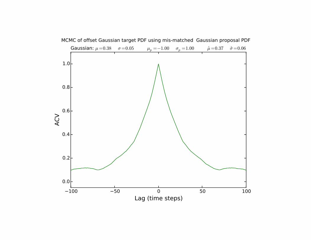
Toy examples of MCMC using Gaussian target and proposal PDFs

The target PDF is N(µ, ⇥2).

For a proposal PDF we use N(µp, ⇥2p) that is wide enough so that values are generated that

overlap with the target PDF. So use

µp = 0 and ⇥p = 3�µ2 + ⇥2

⇥1/2.

In practice, of course, we would not know the parameters of the target PDF (otherwise whatwould be the point of doing MCMC?) and we might not know its support in parameter space.Experimentation may be required to ensure that the parameter space is adequately sampled.

Plots:

Histograms of MC points xt, t = 1, · · · , N for different N and different µ and ⇥.

Autocovariance functions of xt � µx for single realizations that show the correlation time forthe MC time series.

Lessons: the more that the target and proposal PDFs differ, the longer it takes for the time seriesto show stationary statistics that conform to the target PDF. The burn-in time is thus longer insuch cases because it is related to the autocorrelation time.

Example time series are shown for two of the cases that illustrate the burn-in time and thecorrelation time.

9

Histograms

Demonstrate how the distribution of MC points trends to the target PDF!!Target PDF = Gaussian with non-zero mean!!Proposal PDF = N(0, σ2) with σ wide enough to span the target PDF!

�8 �6 �4 �2 0 2 4 6 80.00.51.01.52.02.53.03.54.0

Gaussian: µ = 0.38 ⇥ = 1.29 µ = 0.04 ⇥ = 0.95

�8 �6 �4 �2 0 2 4 6 8012345

Gaussian: µ = 0.38 ⇥ = 1.29 µ = 0.36 ⇥ = 0.91

�8 �6 �4 �2 0 2 4 6 802468101214

Gaussian: µ = 0.38 ⇥ = 1.29 µ = 0.24 ⇥ = 1.36

�8 �6 �4 �2 0 2 4 6 801020304050

Gaussian: µ = 0.38 ⇥ = 1.29 µ = 0.18 ⇥ = 1.34

�8 �6 �4 �2 0 2 4 6 8020406080100120

Gaussian: µ = 0.38 ⇥ = 1.29 µ = 0.37 ⇥ = 1.22

�8 �6 �4 �2 0 2 4 6 8050100150200250300350400

X

Cou

nts

MCMC of offset Gaussian target PDF using zero-mean Gaussian proposal PDF

Gaussian: µ = 0.38 ⇥ = 1.29 µ = 0.31 ⇥ = 1.25

�6 �4 �2 0 2 4 60.0

0.5

1.0

1.5

2.0Gaussian: µ = 1.38 ⇥ = 0.67 µ = 1.18 ⇥ = 0.81

�6 �4 �2 0 2 4 601234567

Gaussian: µ = 1.38 ⇥ = 0.67 µ = 1.53 ⇥ = 0.71

�6 �4 �2 0 2 4 6051015202530

Gaussian: µ = 1.38 ⇥ = 0.67 µ = 1.09 ⇥ = 0.57

�6 �4 �2 0 2 4 6010203040506070

Gaussian: µ = 1.38 ⇥ = 0.67 µ = 1.42 ⇥ = 0.60

�6 �4 �2 0 2 4 6020406080100120140160

Gaussian: µ = 1.38 ⇥ = 0.67 µ = 1.36 ⇥ = 0.74

�6 �4 �2 0 2 4 60

100200300400500600700

X

Cou

nts

MCMC of offset Gaussian target PDF using zero-mean Gaussian proposal PDF

Gaussian: µ = 1.38 ⇥ = 0.67 µ = 1.36 ⇥ = 0.64

�3 �2 �1 0 1 2 30123456

Gaussian: µ = -0.99 ⇥ = 0.33 µ = -1.48 ⇥ = 0.86

�3 �2 �1 0 1 2 30123456789

Gaussian: µ = -0.99 ⇥ = 0.33 µ = -0.89 ⇥ = 0.35

�3 �2 �1 0 1 2 3051015202530

Gaussian: µ = -0.99 ⇥ = 0.33 µ = -0.81 ⇥ = 0.22

�3 �2 �1 0 1 2 30102030405060708090

Gaussian: µ = -0.99 ⇥ = 0.33 µ = -1.01 ⇥ = 0.29

�3 �2 �1 0 1 2 30

50

100

150

200Gaussian: µ = -0.99 ⇥ = 0.33 µ = -0.95 ⇥ = 0.36

�3 �2 �1 0 1 2 30

100200300400500600700

X

Cou

nts

MCMC of offset Gaussian target PDF using zero-mean Gaussian proposal PDF

Gaussian: µ = -0.99 ⇥ = 0.33 µ = -0.99 ⇥ = 0.34

�2.0�1.5�1.0�0.50.0 0.5 1.0 1.5 2.00.00.51.01.52.02.53.0

Gaussian: µ = -0.99 ⇥ = 0.13 µ = -0.84 ⇥ = 0.65

�2.0�1.5�1.0�0.50.0 0.5 1.0 1.5 2.0051015202530

Gaussian: µ = -0.99 ⇥ = 0.13 µ = -0.88 ⇥ = 0.33

�2.0�1.5�1.0�0.50.0 0.5 1.0 1.5 2.0051015202530354045

Gaussian: µ = -0.99 ⇥ = 0.13 µ = -0.84 ⇥ = 0.41

�2.0�1.5�1.0�0.50.0 0.5 1.0 1.5 2.0020406080100120

Gaussian: µ = -0.99 ⇥ = 0.13 µ = -0.98 ⇥ = 0.17

�2.0�1.5�1.0�0.50.0 0.5 1.0 1.5 2.0050100150200250

Gaussian: µ = -0.99 ⇥ = 0.13 µ = -1.00 ⇥ = 0.15

�2.0�1.5�1.0�0.50.0 0.5 1.0 1.5 2.00

2004006008001000

X

Cou

nts

MCMC of offset Gaussian target PDF using zero-mean Gaussian proposal PDF

Gaussian: µ = -0.99 ⇥ = 0.13 µ = -0.99 ⇥ = 0.14

10

Proposal PDF Target PDF

N=8 N=32

N=128

N=2048

N=512

N=8192

�8 �6 �4 �2 0 2 4 6 80.00.51.01.52.02.53.03.54.0

Gaussian: µ = 0.38 ⇥ = 1.29 µ = 0.04 ⇥ = 0.95

�8 �6 �4 �2 0 2 4 6 8012345

Gaussian: µ = 0.38 ⇥ = 1.29 µ = 0.36 ⇥ = 0.91

�8 �6 �4 �2 0 2 4 6 802468101214

Gaussian: µ = 0.38 ⇥ = 1.29 µ = 0.24 ⇥ = 1.36

�8 �6 �4 �2 0 2 4 6 801020304050

Gaussian: µ = 0.38 ⇥ = 1.29 µ = 0.18 ⇥ = 1.34

�8 �6 �4 �2 0 2 4 6 8020406080100120

Gaussian: µ = 0.38 ⇥ = 1.29 µ = 0.37 ⇥ = 1.22

�8 �6 �4 �2 0 2 4 6 8050100150200250300350400

X

Cou

nts

MCMC of offset Gaussian target PDF using zero-mean Gaussian proposal PDF

Gaussian: µ = 0.38 ⇥ = 1.29 µ = 0.31 ⇥ = 1.25

�6 �4 �2 0 2 4 60.0

0.5

1.0

1.5

2.0Gaussian: µ = 1.38 ⇥ = 0.67 µ = 1.18 ⇥ = 0.81

�6 �4 �2 0 2 4 601234567

Gaussian: µ = 1.38 ⇥ = 0.67 µ = 1.53 ⇥ = 0.71

�6 �4 �2 0 2 4 6051015202530

Gaussian: µ = 1.38 ⇥ = 0.67 µ = 1.09 ⇥ = 0.57

�6 �4 �2 0 2 4 6010203040506070

Gaussian: µ = 1.38 ⇥ = 0.67 µ = 1.42 ⇥ = 0.60

�6 �4 �2 0 2 4 6020406080100120140160

Gaussian: µ = 1.38 ⇥ = 0.67 µ = 1.36 ⇥ = 0.74

�6 �4 �2 0 2 4 60

100200300400500600700

X

Cou

nts

MCMC of offset Gaussian target PDF using zero-mean Gaussian proposal PDF

Gaussian: µ = 1.38 ⇥ = 0.67 µ = 1.36 ⇥ = 0.64

�3 �2 �1 0 1 2 30123456

Gaussian: µ = -0.99 ⇥ = 0.33 µ = -1.48 ⇥ = 0.86

�3 �2 �1 0 1 2 30123456789

Gaussian: µ = -0.99 ⇥ = 0.33 µ = -0.89 ⇥ = 0.35

�3 �2 �1 0 1 2 3051015202530

Gaussian: µ = -0.99 ⇥ = 0.33 µ = -0.81 ⇥ = 0.22

�3 �2 �1 0 1 2 30102030405060708090

Gaussian: µ = -0.99 ⇥ = 0.33 µ = -1.01 ⇥ = 0.29

�3 �2 �1 0 1 2 30

50

100

150

200Gaussian: µ = -0.99 ⇥ = 0.33 µ = -0.95 ⇥ = 0.36

�3 �2 �1 0 1 2 30

100200300400500600700

X

Cou

nts

MCMC of offset Gaussian target PDF using zero-mean Gaussian proposal PDF

Gaussian: µ = -0.99 ⇥ = 0.33 µ = -0.99 ⇥ = 0.34

�2.0�1.5�1.0�0.50.0 0.5 1.0 1.5 2.00.00.51.01.52.02.53.0

Gaussian: µ = -0.99 ⇥ = 0.13 µ = -0.84 ⇥ = 0.65

�2.0�1.5�1.0�0.50.0 0.5 1.0 1.5 2.0051015202530

Gaussian: µ = -0.99 ⇥ = 0.13 µ = -0.88 ⇥ = 0.33

�2.0�1.5�1.0�0.50.0 0.5 1.0 1.5 2.0051015202530354045

Gaussian: µ = -0.99 ⇥ = 0.13 µ = -0.84 ⇥ = 0.41

�2.0�1.5�1.0�0.50.0 0.5 1.0 1.5 2.0020406080100120

Gaussian: µ = -0.99 ⇥ = 0.13 µ = -0.98 ⇥ = 0.17

�2.0�1.5�1.0�0.50.0 0.5 1.0 1.5 2.0050100150200250

Gaussian: µ = -0.99 ⇥ = 0.13 µ = -1.00 ⇥ = 0.15

�2.0�1.5�1.0�0.50.0 0.5 1.0 1.5 2.00

2004006008001000

X

Cou

nts

MCMC of offset Gaussian target PDF using zero-mean Gaussian proposal PDF

Gaussian: µ = -0.99 ⇥ = 0.13 µ = -0.99 ⇥ = 0.14

10

Proposal PDF Target PDF

N=8 N=32

N=128

N=2048

N=512

N=8192

Target µ, σ

�8 �6 �4 �2 0 2 4 6 80.00.51.01.52.02.53.03.54.0

Gaussian: µ = 0.38 ⇥ = 1.29 µ = 0.04 ⇥ = 0.95

�8 �6 �4 �2 0 2 4 6 8012345

Gaussian: µ = 0.38 ⇥ = 1.29 µ = 0.36 ⇥ = 0.91

�8 �6 �4 �2 0 2 4 6 802468101214

Gaussian: µ = 0.38 ⇥ = 1.29 µ = 0.24 ⇥ = 1.36

�8 �6 �4 �2 0 2 4 6 801020304050

Gaussian: µ = 0.38 ⇥ = 1.29 µ = 0.18 ⇥ = 1.34

�8 �6 �4 �2 0 2 4 6 8020406080100120

Gaussian: µ = 0.38 ⇥ = 1.29 µ = 0.37 ⇥ = 1.22

�8 �6 �4 �2 0 2 4 6 8050100150200250300350400

X

Cou

nts

MCMC of offset Gaussian target PDF using zero-mean Gaussian proposal PDF

Gaussian: µ = 0.38 ⇥ = 1.29 µ = 0.31 ⇥ = 1.25

�6 �4 �2 0 2 4 60.0

0.5

1.0

1.5

2.0Gaussian: µ = 1.38 ⇥ = 0.67 µ = 1.18 ⇥ = 0.81

�6 �4 �2 0 2 4 601234567

Gaussian: µ = 1.38 ⇥ = 0.67 µ = 1.53 ⇥ = 0.71

�6 �4 �2 0 2 4 6051015202530

Gaussian: µ = 1.38 ⇥ = 0.67 µ = 1.09 ⇥ = 0.57

�6 �4 �2 0 2 4 6010203040506070

Gaussian: µ = 1.38 ⇥ = 0.67 µ = 1.42 ⇥ = 0.60

�6 �4 �2 0 2 4 6020406080100120140160

Gaussian: µ = 1.38 ⇥ = 0.67 µ = 1.36 ⇥ = 0.74

�6 �4 �2 0 2 4 60

100200300400500600700

X

Cou

nts

MCMC of offset Gaussian target PDF using zero-mean Gaussian proposal PDF

Gaussian: µ = 1.38 ⇥ = 0.67 µ = 1.36 ⇥ = 0.64

�3 �2 �1 0 1 2 30123456

Gaussian: µ = -0.99 ⇥ = 0.33 µ = -1.48 ⇥ = 0.86

�3 �2 �1 0 1 2 30123456789

Gaussian: µ = -0.99 ⇥ = 0.33 µ = -0.89 ⇥ = 0.35

�3 �2 �1 0 1 2 3051015202530

Gaussian: µ = -0.99 ⇥ = 0.33 µ = -0.81 ⇥ = 0.22

�3 �2 �1 0 1 2 30102030405060708090

Gaussian: µ = -0.99 ⇥ = 0.33 µ = -1.01 ⇥ = 0.29

�3 �2 �1 0 1 2 30

50

100

150

200Gaussian: µ = -0.99 ⇥ = 0.33 µ = -0.95 ⇥ = 0.36

�3 �2 �1 0 1 2 30

100200300400500600700

X

Cou

nts

MCMC of offset Gaussian target PDF using zero-mean Gaussian proposal PDF

Gaussian: µ = -0.99 ⇥ = 0.33 µ = -0.99 ⇥ = 0.34

�2.0�1.5�1.0�0.50.0 0.5 1.0 1.5 2.00.00.51.01.52.02.53.0

Gaussian: µ = -0.99 ⇥ = 0.13 µ = -0.84 ⇥ = 0.65

�2.0�1.5�1.0�0.50.0 0.5 1.0 1.5 2.0051015202530

Gaussian: µ = -0.99 ⇥ = 0.13 µ = -0.88 ⇥ = 0.33

�2.0�1.5�1.0�0.50.0 0.5 1.0 1.5 2.0051015202530354045

Gaussian: µ = -0.99 ⇥ = 0.13 µ = -0.84 ⇥ = 0.41

�2.0�1.5�1.0�0.50.0 0.5 1.0 1.5 2.0020406080100120

Gaussian: µ = -0.99 ⇥ = 0.13 µ = -0.98 ⇥ = 0.17

�2.0�1.5�1.0�0.50.0 0.5 1.0 1.5 2.0050100150200250

Gaussian: µ = -0.99 ⇥ = 0.13 µ = -1.00 ⇥ = 0.15

�2.0�1.5�1.0�0.50.0 0.5 1.0 1.5 2.00

2004006008001000

X

Cou

nts

MCMC of offset Gaussian target PDF using zero-mean Gaussian proposal PDF

Gaussian: µ = -0.99 ⇥ = 0.13 µ = -0.99 ⇥ = 0.14

10

Proposal PDF Target PDF

N=8 N=32

N=128

N=2048

N=512

N=8192

Target µ, σ µ, σ from MC values

Four cases with different target PDFs!!Even for target PDFs with large means, we obtain convergence. !

�8 �6 �4 �2 0 2 4 6 80.00.51.01.52.02.53.03.54.0

Gaussian: µ = 0.38 ⇥ = 1.29 µ = 0.04 ⇥ = 0.95

�8 �6 �4 �2 0 2 4 6 8012345

Gaussian: µ = 0.38 ⇥ = 1.29 µ = 0.36 ⇥ = 0.91

�8 �6 �4 �2 0 2 4 6 802468101214

Gaussian: µ = 0.38 ⇥ = 1.29 µ = 0.24 ⇥ = 1.36

�8 �6 �4 �2 0 2 4 6 801020304050

Gaussian: µ = 0.38 ⇥ = 1.29 µ = 0.18 ⇥ = 1.34

�8 �6 �4 �2 0 2 4 6 8020406080100120

Gaussian: µ = 0.38 ⇥ = 1.29 µ = 0.37 ⇥ = 1.22

�8 �6 �4 �2 0 2 4 6 8050100150200250300350400

X

Cou

nts

MCMC of offset Gaussian target PDF using zero-mean Gaussian proposal PDF

Gaussian: µ = 0.38 ⇥ = 1.29 µ = 0.31 ⇥ = 1.25

�6 �4 �2 0 2 4 60.0

0.5

1.0

1.5

2.0Gaussian: µ = 1.38 ⇥ = 0.67 µ = 1.18 ⇥ = 0.81

�6 �4 �2 0 2 4 601234567

Gaussian: µ = 1.38 ⇥ = 0.67 µ = 1.53 ⇥ = 0.71

�6 �4 �2 0 2 4 6051015202530

Gaussian: µ = 1.38 ⇥ = 0.67 µ = 1.09 ⇥ = 0.57

�6 �4 �2 0 2 4 6010203040506070

Gaussian: µ = 1.38 ⇥ = 0.67 µ = 1.42 ⇥ = 0.60

�6 �4 �2 0 2 4 6020406080100120140160

Gaussian: µ = 1.38 ⇥ = 0.67 µ = 1.36 ⇥ = 0.74

�6 �4 �2 0 2 4 60

100200300400500600700

X

Cou

nts

MCMC of offset Gaussian target PDF using zero-mean Gaussian proposal PDF

Gaussian: µ = 1.38 ⇥ = 0.67 µ = 1.36 ⇥ = 0.64

�3 �2 �1 0 1 2 30123456

Gaussian: µ = -0.99 ⇥ = 0.33 µ = -1.48 ⇥ = 0.86

�3 �2 �1 0 1 2 30123456789

Gaussian: µ = -0.99 ⇥ = 0.33 µ = -0.89 ⇥ = 0.35

�3 �2 �1 0 1 2 3051015202530

Gaussian: µ = -0.99 ⇥ = 0.33 µ = -0.81 ⇥ = 0.22

�3 �2 �1 0 1 2 30102030405060708090

Gaussian: µ = -0.99 ⇥ = 0.33 µ = -1.01 ⇥ = 0.29

�3 �2 �1 0 1 2 30

50

100

150

200Gaussian: µ = -0.99 ⇥ = 0.33 µ = -0.95 ⇥ = 0.36

�3 �2 �1 0 1 2 30

100200300400500600700

X

Cou

nts

MCMC of offset Gaussian target PDF using zero-mean Gaussian proposal PDF

Gaussian: µ = -0.99 ⇥ = 0.33 µ = -0.99 ⇥ = 0.34

�2.0�1.5�1.0�0.50.0 0.5 1.0 1.5 2.00.00.51.01.52.02.53.0

Gaussian: µ = -0.99 ⇥ = 0.13 µ = -0.84 ⇥ = 0.65

�2.0�1.5�1.0�0.50.0 0.5 1.0 1.5 2.0051015202530

Gaussian: µ = -0.99 ⇥ = 0.13 µ = -0.88 ⇥ = 0.33

�2.0�1.5�1.0�0.50.0 0.5 1.0 1.5 2.0051015202530354045

Gaussian: µ = -0.99 ⇥ = 0.13 µ = -0.84 ⇥ = 0.41

�2.0�1.5�1.0�0.50.0 0.5 1.0 1.5 2.0020406080100120

Gaussian: µ = -0.99 ⇥ = 0.13 µ = -0.98 ⇥ = 0.17

�2.0�1.5�1.0�0.50.0 0.5 1.0 1.5 2.0050100150200250

Gaussian: µ = -0.99 ⇥ = 0.13 µ = -1.00 ⇥ = 0.15

�2.0�1.5�1.0�0.50.0 0.5 1.0 1.5 2.00

2004006008001000

X

Cou

nts

MCMC of offset Gaussian target PDF using zero-mean Gaussian proposal PDF

Gaussian: µ = -0.99 ⇥ = 0.13 µ = -0.99 ⇥ = 0.14

10

Note only 2 states for 1st 8 MC samples

�1.5 �1.0 �0.5 0.0 0.5 1.0 1.50123456

Gaussian: µ = -0.99 ⇥ = 0.05 µ = -0.45 ⇥ = 0.77

�1.5 �1.0 �0.5 0.0 0.5 1.0 1.501234567

Gaussian: µ = -0.99 ⇥ = 0.05 µ = -1.24 ⇥ = 0.37

�1.5 �1.0 �0.5 0.0 0.5 1.0 1.5010203040506070

Gaussian: µ = -0.99 ⇥ = 0.05 µ = -0.90 ⇥ = 0.15

�1.5 �1.0 �0.5 0.0 0.5 1.0 1.50

50

100

150

200Gaussian: µ = -0.99 ⇥ = 0.05 µ = -0.97 ⇥ = 0.17

�1.5 �1.0 �0.5 0.0 0.5 1.0 1.50

100200300400500600700

Gaussian: µ = -0.99 ⇥ = 0.05 µ = -1.00 ⇥ = 0.10

�1.5 �1.0 �0.5 0.0 0.5 1.0 1.50

500

1000

1500

2000

X

Cou

nts

MCMC of offset Gaussian target PDF using zero-mean Gaussian proposal PDF

Gaussian: µ = -0.99 ⇥ = 0.05 µ = -0.99 ⇥ = 0.08

11

Narrow target PDF

�6 �4 �2 0 2 4 60.0

0.5

1.0

1.5

2.0Gaussian: µ = 1.38 � = 0.67 µ = 1.18 � = 0.81

�6 �4 �2 0 2 4 601234567

Gaussian: µ = 1.38 � = 0.67 µ = 1.53 � = 0.71

�6 �4 �2 0 2 4 605

1015202530

Gaussian: µ = 1.38 � = 0.67 µ = 1.09 � = 0.57

�6 �4 �2 0 2 4 60

10203040506070

Gaussian: µ = 1.38 � = 0.67 µ = 1.42 � = 0.60

�6 �4 �2 0 2 4 60

20406080

100120140160

Gaussian: µ = 1.38 � = 0.67 µ = 1.36 � = 0.74

�6 �4 �2 0 2 4 60

100200300400500600700

X

Cou

nts

MCMC of offset Gaussian target PDF using zero-mean Gaussian proposal PDF

Gaussian: µ = 1.38 � = 0.67 µ = 1.36 � = 0.64

Broader target PDF

�8 �6 �4 �2 0 2 4 6 80.00.51.01.52.02.53.03.54.0

Gaussian: µ = 0.38 � = 1.29 µ = 0.04 � = 0.95

�8 �6 �4 �2 0 2 4 6 8012345

Gaussian: µ = 0.38 � = 1.29 µ = 0.36 � = 0.91

�8 �6 �4 �2 0 2 4 6 802468

101214

Gaussian: µ = 0.38 � = 1.29 µ = 0.24 � = 1.36

�8 �6 �4 �2 0 2 4 6 80

1020304050

Gaussian: µ = 0.38 � = 1.29 µ = 0.18 � = 1.34

�8 �6 �4 �2 0 2 4 6 80

20406080

100120

Gaussian: µ = 0.38 � = 1.29 µ = 0.37 � = 1.22

�8 �6 �4 �2 0 2 4 6 80

50100150200250300350400

X

Cou

nts

MCMC of offset Gaussian target PDF using zero-mean Gaussian proposal PDF

Gaussian: µ = 0.38 � = 1.29 µ = 0.31 � = 1.25

Even broader target PDF

Proposal PDF proportionately broader

�3 �2 �1 0 1 2 30123456

Gaussian: µ = -0.99 � = 0.33 µ = -1.48 � = 0.86

�3 �2 �1 0 1 2 30123456789

Gaussian: µ = -0.99 � = 0.33 µ = -0.89 � = 0.35

�3 �2 �1 0 1 2 305

1015202530

Gaussian: µ = -0.99 � = 0.33 µ = -0.81 � = 0.22

�3 �2 �1 0 1 2 30

102030405060708090

Gaussian: µ = -0.99 � = 0.33 µ = -1.01 � = 0.29

�3 �2 �1 0 1 2 30

50

100

150

200Gaussian: µ = -0.99 � = 0.33 µ = -0.95 � = 0.36

�3 �2 �1 0 1 2 30

100200300400500600700

X

Cou

nts

MCMC of offset Gaussian target PDF using zero-mean Gaussian proposal PDF

Gaussian: µ = -0.99 � = 0.33 µ = -0.99 � = 0.34

Sequence of progressively narrower target PDFs

�2.0�1.5�1.0�0.50.0 0.5 1.0 1.5 2.00.00.51.01.52.02.53.0

Gaussian: µ = -0.99 � = 0.13 µ = -0.84 � = 0.65

�2.0�1.5�1.0�0.50.0 0.5 1.0 1.5 2.005

1015202530

Gaussian: µ = -0.99 � = 0.13 µ = -0.88 � = 0.33

�2.0�1.5�1.0�0.50.0 0.5 1.0 1.5 2.005

1015202530354045

Gaussian: µ = -0.99 � = 0.13 µ = -0.84 � = 0.41

�2.0�1.5�1.0�0.50.0 0.5 1.0 1.5 2.00

20406080

100120

Gaussian: µ = -0.99 � = 0.13 µ = -0.98 � = 0.17

�2.0�1.5�1.0�0.50.0 0.5 1.0 1.5 2.00

50100150200250

Gaussian: µ = -0.99 � = 0.13 µ = -1.00 � = 0.15

�2.0�1.5�1.0�0.50.0 0.5 1.0 1.5 2.00

200400600800

1000

X

Cou

nts

MCMC of offset Gaussian target PDF using zero-mean Gaussian proposal PDF

Gaussian: µ = -0.99 � = 0.13 µ = -0.99 � = 0.14

�1.5 �1.0 �0.5 0.0 0.5 1.0 1.50123456

Gaussian: µ = -0.99 � = 0.05 µ = -0.45 � = 0.77

�1.5 �1.0 �0.5 0.0 0.5 1.0 1.501234567

Gaussian: µ = -0.99 � = 0.05 µ = -1.24 � = 0.37

�1.5 �1.0 �0.5 0.0 0.5 1.0 1.50

10203040506070

Gaussian: µ = -0.99 � = 0.05 µ = -0.90 � = 0.15

�1.5 �1.0 �0.5 0.0 0.5 1.0 1.50

50

100

150

200Gaussian: µ = -0.99 � = 0.05 µ = -0.97 � = 0.17

�1.5 �1.0 �0.5 0.0 0.5 1.0 1.50

100200300400500600700

Gaussian: µ = -0.99 � = 0.05 µ = -1.00 � = 0.10

�1.5 �1.0 �0.5 0.0 0.5 1.0 1.50

500

1000

1500

2000

X

Cou

nts

MCMC of offset Gaussian target PDF using zero-mean Gaussian proposal PDF

Gaussian: µ = -0.99 � = 0.05 µ = -0.99 � = 0.08

ACFs of MCMC-generated Time Series

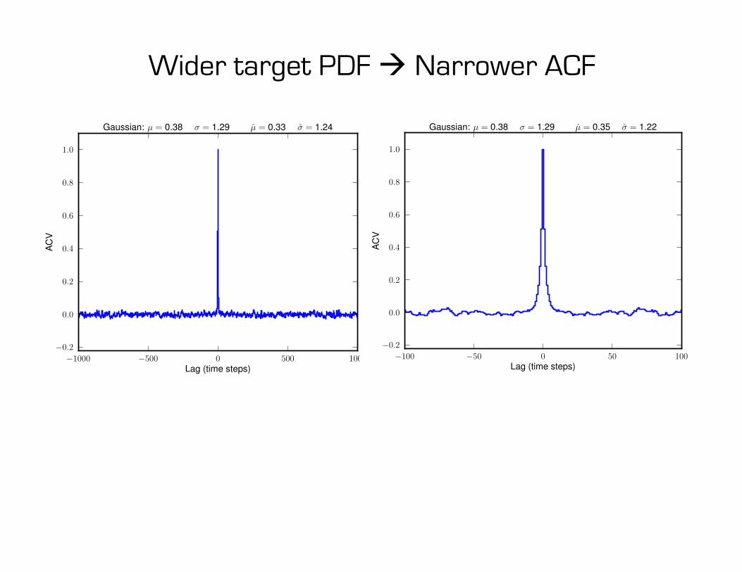
•  Width of ACF = correlation time for the time series!

•  Too long a correlation time à inefficient sampling of parameter space!

•  Longer correlation times correspond to proposal PDFs that have larger support relative to the support of the target PDF.!

!

0 200 400 600 800 1000Time (steps)

�4

�2

0

2

4

Tim

eS

erie

s

Gaussian: µ = 0.38 � = 1.29 µ = 0.23 � = 1.20

Time Series of MCMC Samples Case with wide target PDF

0 2000 4000 6000 8000 10000Time (steps)

�1.2

�1.0

�0.8

�0.6

�0.4

�0.2

0.0

0.2

Tim

eS

erie

s

Gaussian: µ = -0.99 � = 0.05 µ = -0.99 � = 0.06

0 200 400 600 800 1000Time (steps)

�1.2

�1.0

�0.8

�0.6

�0.4

�0.2

0.0

0.2

Tim

eS

erie

s

Gaussian: µ = -0.99 � = 0.05 µ = -1.00 � = 0.07

Time Series of MCMC Samples Case with narrow target PDF

Burn-in time

�100 �50 0 50 100Lag (time steps)

�0.2

0.0

0.2

0.4

0.6

0.8

1.0

ACV

Gaussian: µ = 1.38 � = 1.67 µ = 1.30 � = 1.58

Full ACF

Zoom in to inner 10% (same case, different realization)

�1000 �500 0 500 1000Lag (time steps)

�0.2

0.0

0.2

0.4

0.6

0.8

1.0

ACV

Gaussian: µ = 1.38 � = 1.67 µ = 1.31 � = 1.62

�1000 �500 0 500 1000Lag (time steps)

�0.2

0.0

0.2

0.4

0.6

0.8

1.0

ACV

Gaussian: µ = 1.38 � = 0.67 µ = 1.34 � = 0.67

�100 �50 0 50 100Lag (time steps)

�0.2

0.0

0.2

0.4

0.6

0.8

1.0

ACV

Gaussian: µ = 1.38 � = 0.67 µ = 1.35 � = 0.70

Relatively wide target PDF

�1000 �500 0 500 1000Lag (time steps)

�0.2

0.0

0.2

0.4

0.6

0.8

1.0

ACV

Gaussian: µ = 0.38 � = 1.29 µ = 0.33 � = 1.24

�100 �50 0 50 100Lag (time steps)

�0.2

0.0

0.2

0.4

0.6

0.8

1.0

ACV

Gaussian: µ = 0.38 � = 1.29 µ = 0.35 � = 1.22

Wider target PDF à Narrower ACF

�1000 �500 0 500 1000Lag (time steps)

�0.2

0.0

0.2

0.4

0.6

0.8

1.0

ACV

Gaussian: µ = -0.99 � = 0.33 µ = -0.98 � = 0.34

Narrower target PDF à Wider ACF

�1000 �500 0 500 1000Lag (time steps)

�0.2

0.0

0.2

0.4

0.6

0.8

1.0

ACV

Gaussian: µ = -0.99 � = 0.13 µ = -0.99 � = 0.13

Narrower target PDF à Wider ACF

�1000 �500 0 500 1000Lag (time steps)

�0.2

0.0

0.2

0.4

0.6

0.8

1.0

ACV

Gaussian: µ = -0.99 � = 0.05 µ = -0.99 � = 0.05

Narrower target PDF à Wider ACF

Unsuitable Proposal PDFs