A6523 Signal Modeling, Statistical Inference and Data

Mining in Astrophysics Spring 2013

Lecture 2 •  For next week read Chapter 1 of Gregory (Role of Probability in Science) •  Web page for course is www.astro.cornell.edu/~cordes/A6523 and it is now

being linked to the Astronomy web page.

•  Today: a whirlwind tour through linear systems and Fourier transforms. Details will come later.

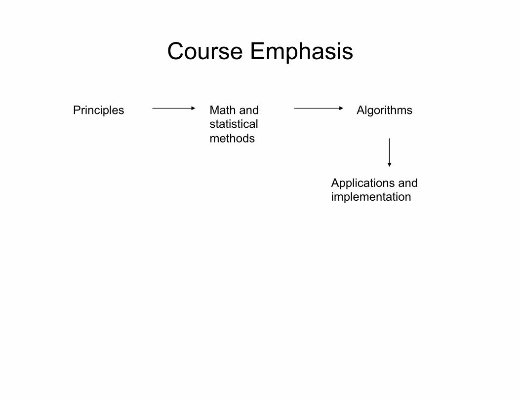
Course Emphasis

Principles Math and statistical methods

Algorithms

Applications and implementation

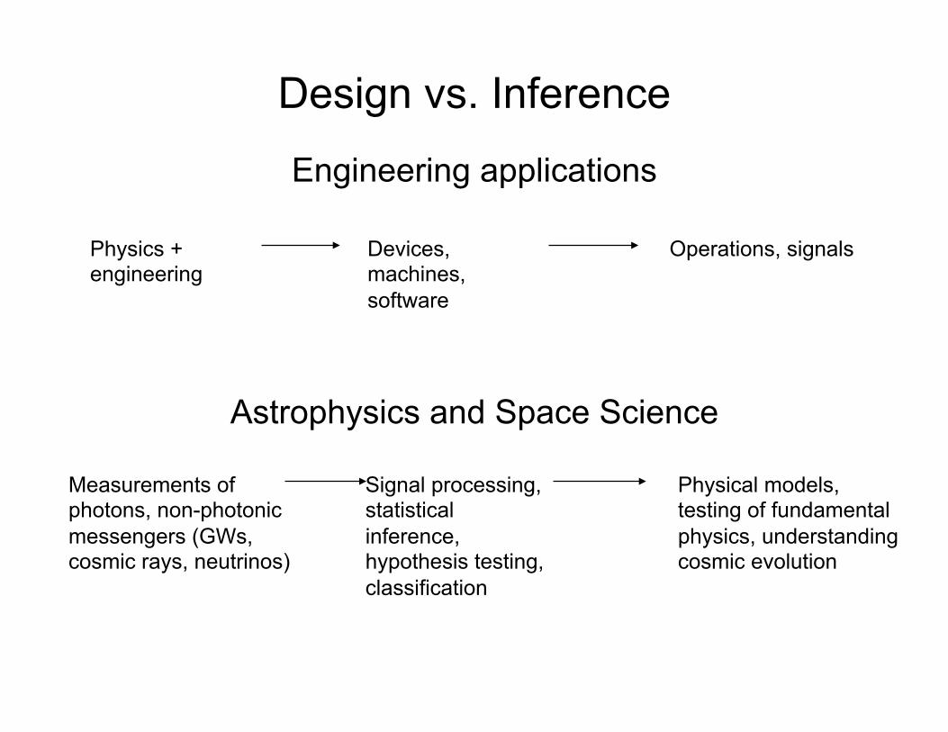
Design vs. Inference

Engineering applications

Astrophysics and Space Science

Physics + engineering

Devices, machines, software

Operations, signals

Measurements of photons, non-photonic messengers (GWs, cosmic rays, neutrinos)

Signal processing, statistical inference, hypothesis testing, classification

Physical models, testing of fundamental physics, understanding cosmic evolution

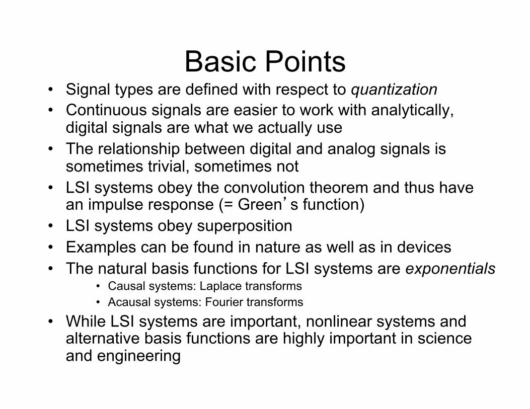
Basic Points •  Signal types are defined with respect to quantization •  Continuous signals are easier to work with analytically,

digital signals are what we actually use •  The relationship between digital and analog signals is

sometimes trivial, sometimes not •  LSI systems obey the convolution theorem and thus have

an impulse response (= Green’s function) •  LSI systems obey superposition •  Examples can be found in nature as well as in devices •  The natural basis functions for LSI systems are exponentials

•  Causal systems: Laplace transforms •  Acausal systems: Fourier transforms

•  While LSI systems are important, nonlinear systems and alternative basis functions are highly important in science and engineering

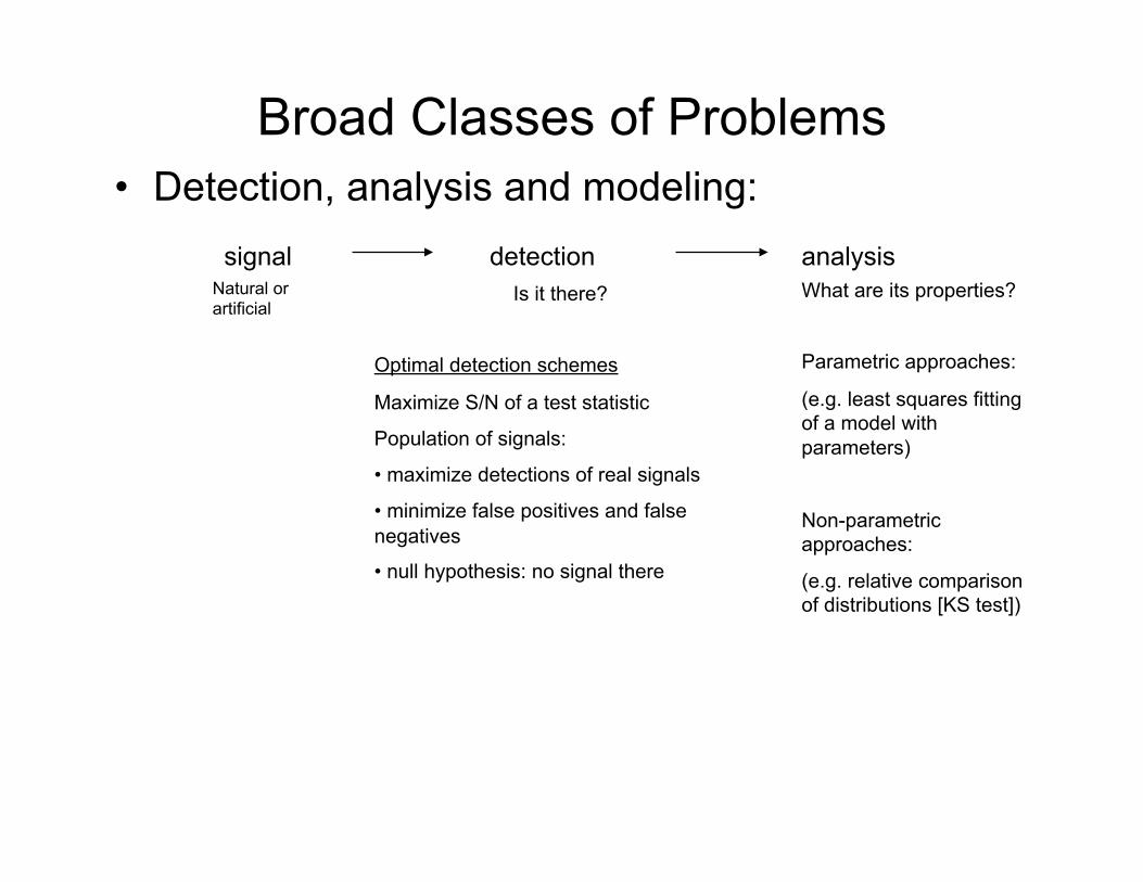
Broad Classes of Problems •  Detection, analysis and modeling:

signal detection analysis Natural or artificial

Is it there?

Optimal detection schemes

Maximize S/N of a test statistic

Population of signals:

•  maximize detections of real signals

•  minimize false positives and false negatives

•  null hypothesis: no signal there

What are its properties?

Parametric approaches:

(e.g. least squares fitting of a model with parameters)

Non-parametric approaches:

(e.g. relative comparison of distributions [KS test])

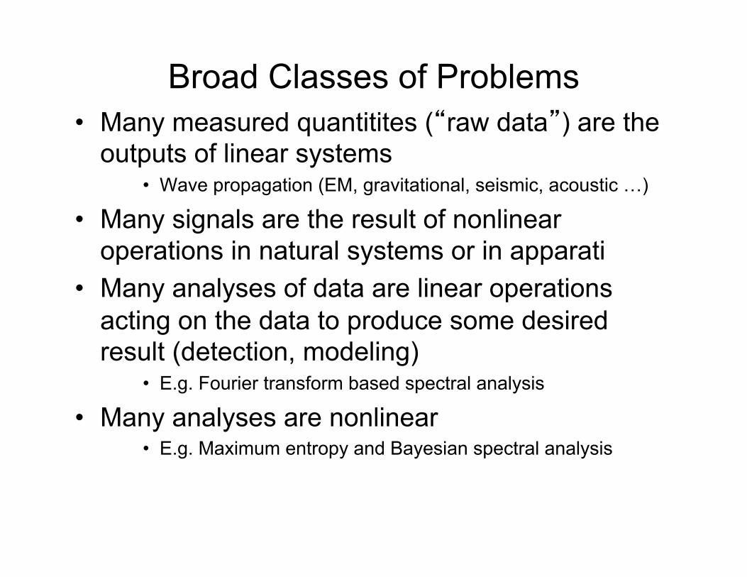
Broad Classes of Problems •  Many measured quantitites (“raw data”) are the

outputs of linear systems •  Wave propagation (EM, gravitational, seismic, acoustic !)

•  Many signals are the result of nonlinear operations in natural systems or in apparati

•  Many analyses of data are linear operations acting on the data to produce some desired result (detection, modeling)

•  E.g. Fourier transform based spectral analysis

•  Many analyses are nonlinear •  E.g. Maximum entropy and Bayesian spectral analysis

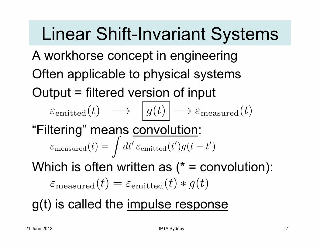
Linear Shift-Invariant Systems A workhorse concept in engineering Often applicable to physical systems Output = filtered version of input “Filtering” means convolution:

Which is often written as (* = convolution): g(t) is called the impulse response

21 June 2012 IPTA Sydney 7

εemitted(t) −→ g(t) −→ εmeasured(t)

εmeasured(t) =

�dt� εemitted(t

�)g(t− t�)

εmeasured(t) = εemitted(t) ∗ g(t)

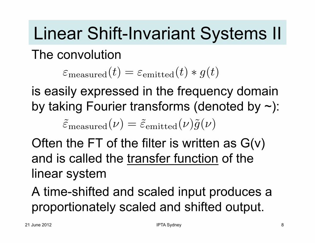
Linear Shift-Invariant Systems II The convolution is easily expressed in the frequency domain by taking Fourier transforms (denoted by ~): Often the FT of the filter is written as G(!) and is called the transfer function of the linear system A time-shifted and scaled input produces a proportionately scaled and shifted output. 21 June 2012 IPTA Sydney 8

εmeasured(t) = εemitted(t) ∗ g(t)

εmeasured(ν) = εemitted(ν)g(ν)

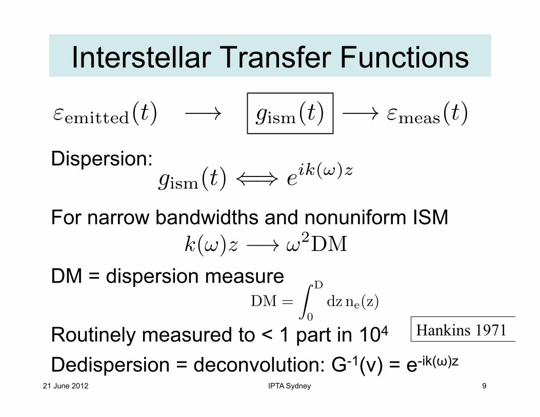
Interstellar Transfer Functions

Dispersion: For narrow bandwidths and nonuniform ISM DM = dispersion measure Routinely measured to < 1 part in 104

Dedispersion = deconvolution: G-1(!) = e-ik(")z 21 June 2012 IPTA Sydney 9

k(ω)z −→ ω2DM

DM =

� D

0dz ne(z)

εemitted(t) −→ gism(t) −→ εmeas(t)

gism(t) ⇐⇒ eik(ω)z

Hankins 1971

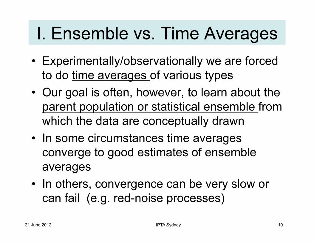
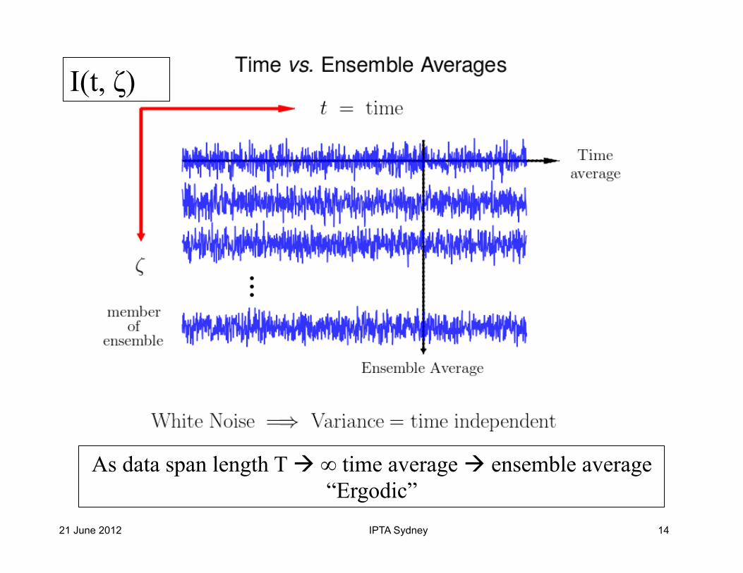
I. Ensemble vs. Time Averages •  Experimentally/observationally we are forced

to do time averages of various types •  Our goal is often, however, to learn about the

parent population or statistical ensemble from which the data are conceptually drawn

•  In some circumstances time averages converge to good estimates of ensemble averages

•  In others, convergence can be very slow or can fail (e.g. red-noise processes)

21 June 2012 IPTA Sydney 10

Example: the Universe •  Measurements of the CMB and large-scale structure

are on a single realization •  The goal of cosmology is to learn about the (notional)

ensemble of conditions that lead to what we see

•  Quantitatively these are cast in questions like “what was the primordial spectrum of density fluctuations?” and that spectrum is usually parameterized as a power law

•  Perhaps the multiverse = the ensemble •  Are all universes the same (statistically)? •  Do measurements on our universe typify all

universes? (Conventional wisdom says no) 21 June 2012 IPTA Sydney 11

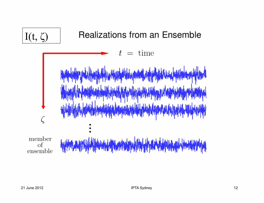
21 June 2012 IPTA Sydney 12

I(t, !)

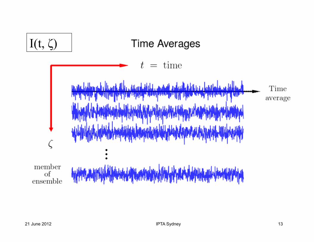
21 June 2012 IPTA Sydney 13

I(t, !)

21 June 2012 IPTA Sydney 14

As data span length T ! ! time average ! ensemble average “Ergodic”

I(t, ")

A6523

Linear, Shift-invariant Systems, Fourier Transforms,and Some Detection Issues

• Linear systems underly much of what happens in nature and are used in instrumentation to makemeasurements of various kinds.

• We will define linear systems formally and derive some properties.

• We will show that exponentials are natural basis functions for describing linear systems.

• Fourier transforms (CT/CA), Fourier Series (CT/CA + periodic in time), and Discrete FourierTransforms (DT/CA + periodic in time and in frequency) will be defined.

• We will look at an application that demonstrates:

1. Definition of a power spectrum from the DFT.2. Statistics of the power spectrum and how we generally can derive statistics for any estimator or

test statistic.3. The notion of an ensemble or parent population from which a given set of measurements is

drawn (a realization of the process).4. Investigate a “detection” problem (finding a weak signal in noise) and assess the false-alarm

probability.

1

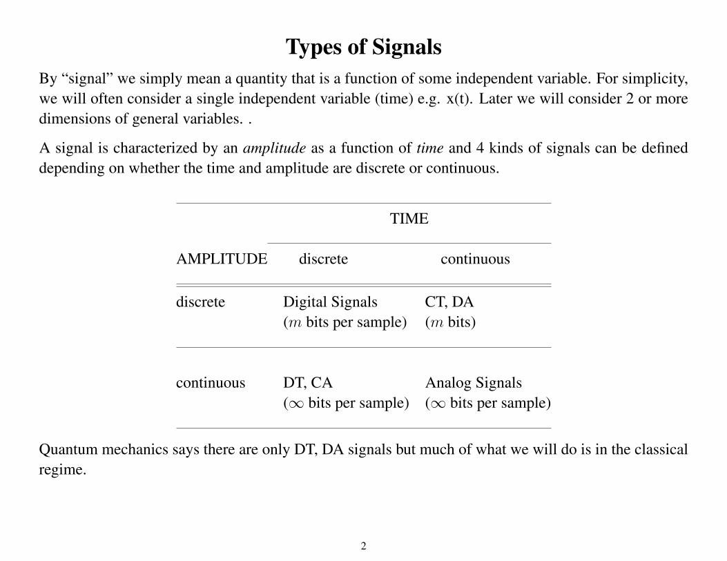
Types of SignalsBy “signal” we simply mean a quantity that is a function of some independent variable. For simplicity,we will often consider a single independent variable (time) e.g. x(t). Later we will consider 2 or moredimensions of general variables. .

A signal is characterized by an amplitude as a function of time and 4 kinds of signals can be defineddepending on whether the time and amplitude are discrete or continuous.

TIME

AMPLITUDE discrete continuous

discrete Digital Signals CT, DA(m bits per sample) (m bits)

continuous DT, CA Analog Signals(∞ bits per sample) (∞ bits per sample)

Quantum mechanics says there are only DT, DA signals but much of what we will do is in the classicalregime.

2

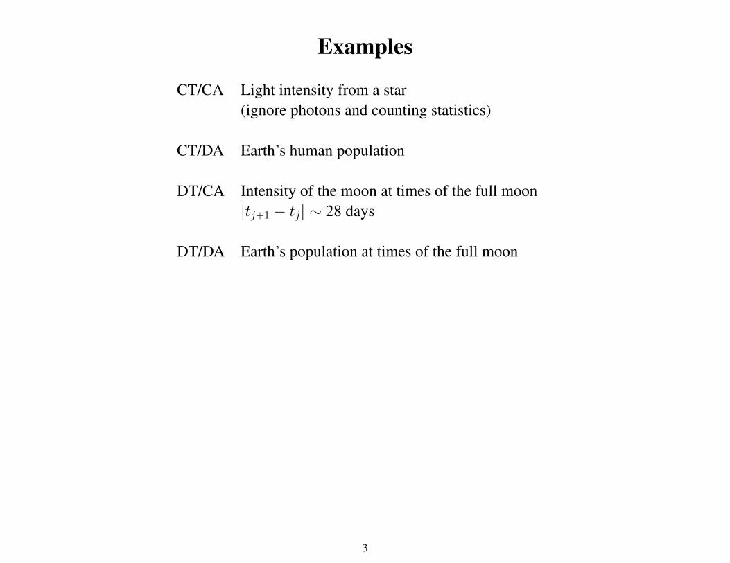
Examples

CT/CA Light intensity from a star(ignore photons and counting statistics)

CT/DA Earth’s human population

DT/CA Intensity of the moon at times of the full moon|tj+1 − tj| ∼ 28 days

DT/DA Earth’s population at times of the full moon

3

Approach taken in the courseTheoretical treatments (analytical results) will generally be applied to DT/CA signals, for simplicity.

For the most part, we will consider analog signals and DT/CA signals, the latter as an approximationto digital signals. For most analyses, the discreteness in time is a strong influence on what we can inferfrom the data. Discreteness in amplitude is not so important, except insofar as it represents a source oferror (quantization noise). However, we will consider the case of extreme quantization into one bit ofinformation and derive estimators of the autocovariance.

Generically, we refer to a DT signal as a time series and the set of all possible analyses as “time seriesanalysis”. However, most of what we do is applicable to any sequence of data, regardless of what theindependent variable is.

Often, but not always, we can consider a DT signal to be a sampled version of a CT signal (counterexamples: occurrence times of discrete events such as clock ticks, heartbeats, photon impacts, etc.).

Nonuniform sampling often occurs and has a major impact on the structure of an algorithm.

We will consider the effects of quantization in digital signals.

4

Linear SystemsConsider a linear differential equation in y

f (y, y�, y

��, . . .) = x(t), y

� ≡ dy

dt, etc.

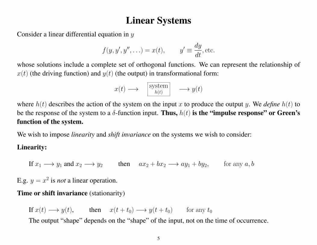
whose solutions include a complete set of orthogonal functions. We can represent the relationship ofx(t) (the driving function) and y(t) (the output) in transformational form:

x(t) −→ systemh(t) −→ y(t)

where h(t) describes the action of the system on the input x to produce the output y. We define h(t) tobe the response of the system to a δ-function input. Thus, h(t) is the “impulse response” or Green’sfunction of the system.

We wish to impose linearity and shift invariance on the systems we wish to consider:

Linearity:

If x1 −→ y1 and x2 −→ y2 then ax2 + bx2 −→ ay1 + by2, for any a, b

E.g. y = x2 is not a linear operation.

Time or shift invariance (stationarity)

If x(t) −→ y(t), then x(t + t0) −→ y(t + t0) for any t0

The output “shape” depends on the “shape” of the input, not on the time of occurrence.

5

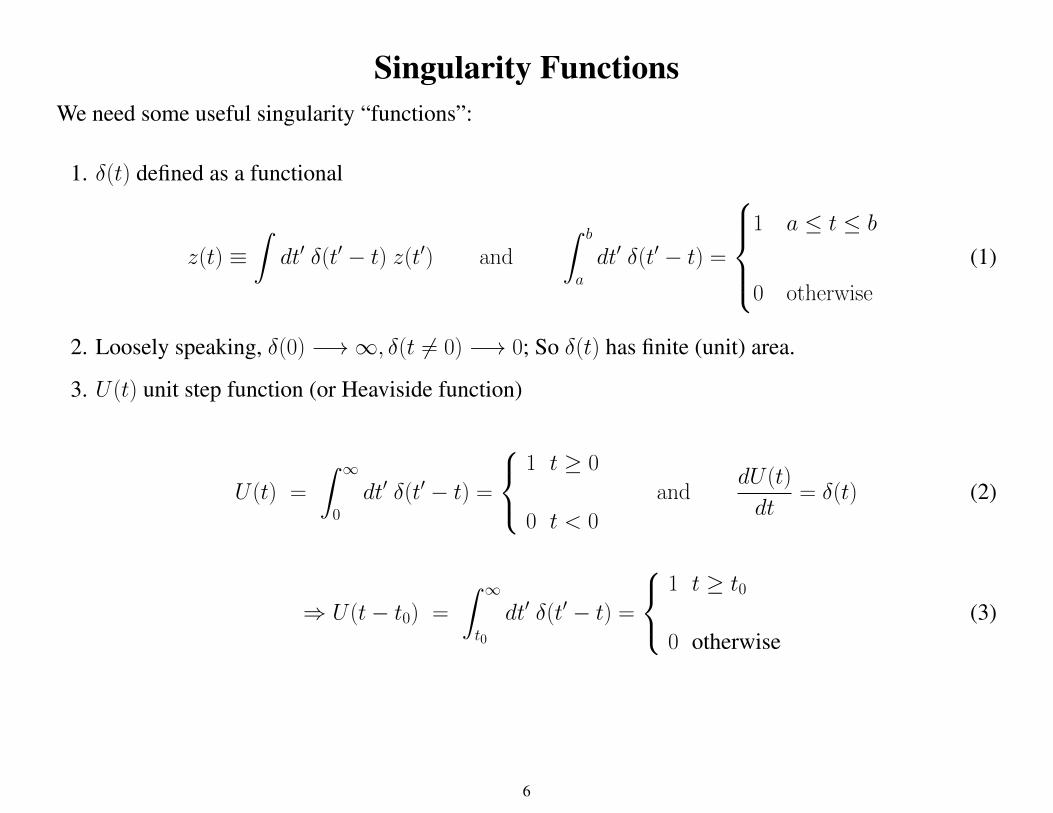
Singularity FunctionsWe need some useful singularity “functions”:

1. δ(t) defined as a functional

z(t) ≡�

dt� δ(t� − t) z(t

�) and

�b

a

dt� δ(t� − t) =

1 a ≤ t ≤ b

0 otherwise

(1)

2. Loosely speaking, δ(0) −→ ∞, δ(t �= 0) −→ 0; So δ(t) has finite (unit) area.

3. U(t) unit step function (or Heaviside function)

U(t) =

� ∞

0dt

� δ(t� − t) =

1 t ≥ 0

0 t < 0

anddU(t)

dt= δ(t) (2)

⇒ U(t− t0) =

� ∞

t0

dt� δ(t� − t) =

1 t ≥ t0

0 otherwise(3)

6

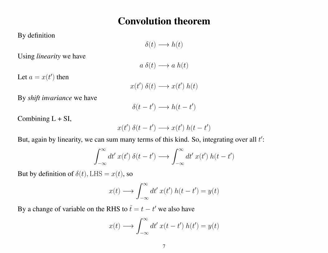
Convolution theoremBy definition

δ(t) −→ h(t)

Using linearity we havea δ(t) −→ a h(t)

Let a = x(t�) then

x(t�) δ(t) −→ x(t

�) h(t)

By shift invariance we haveδ(t− t

�) −→ h(t− t

�)

Combining L + SI,x(t

�) δ(t− t

�) −→ x(t

�) h(t− t

�)

But, again by linearity, we can sum many terms of this kind. So, integrating over all t�:� ∞

−∞dt

�x(t

�) δ(t− t

�) −→

� ∞

−∞dt

�x(t

�) h(t− t

�)

But by definition of δ(t),LHS = x(t), so

x(t) −→� ∞

−∞dt

�x(t

�) h(t− t

�) = y(t)

By a change of variable on the RHS to t = t− t� we also have

x(t) −→� ∞

−∞dt

�x(t− t

�) h(t

�) = y(t)

7

Any linear, shift invariant system can be described as the convolu-tion of its impulse response with an arbitrary input.Using the notation ∗ to represent the integration, we therefore have

y(t) = x ∗ h = h ∗ x

Properties:

1. Convolution commutes:�

dt�h(t

�)x(t− t

�) =

�dt

�h(t− t

�)x(t

�)

2. Graphically, convolution is “invert, slide, and sum”

3. The general integral form of ∗ implies that, usually, information about the input is lost since h(t)

can “smear out” or otherwise preferentially weight portions of the input.

4. Theoretically, if the system response h(t) is known, the output can be ‘deconvolved’ to obtain theinput. But this is unsuccessful in many practical cases because: a) the system h(t) is not known toarbitrary precision or, b) the output is not known to arbitrary precision.

8

Why are linear systems useful?

1. Filtering (real time, offline, analog, digital, causal, acausal)

2. Much signal processing and data analysis consists of the application of a linear operator (smooth-ing, running means, Fourier transforms, generalized channelization, ... )

3. Natural processes can often be described as linear systems:

• Response of the Earth to an earthquake (propagation of seismic waves)• Response of an active galactic nucleus swallowing a star (models for quasar light curves)• Calculating the radiation pattern from an ensemble of particles• Propagation of electromagnetic pulses through plasmas• Radiation from gravitational wave sources (in weak-field regime)

9

We want to be able to attack the following kinds of problems:

1. Algorithm development: Given h(t), how do we get y(t) given x(t) (“how” meaning to obtainefficiently, hardware vs. software, etc.) t vs. f domain?

2. Estimation: To achieve a certain kind of output, such as parameter estimates subject to “con-straints”(e.g. minimum square error), how do we design h(t)? (least squares estimation, prediction,interpolation)

3. Inverse Theory: Given the output (e.g. a measured signal) and assumptions about the input, howwell can we determine h(t) (parameter estimation)? How well can we determine the original inputx(t)? Usually the output is corrupted by noise, so we have

y(t) = h(t) ∗ x(t) + �(t).

The extent to which we can determine h and x depends on the signal-to-noise ratio:�(h ∗ x)2�1/2/��2�1/2 where � � denotes averaging brackets.We also need to consider deterministic, chaotic and stochastic systems:

• Deterministic ⇒ predictable, precise (noiseless) functions• Chaotic ⇒ deterministic but apparently stochastic processes• Stochastic ⇒ not predictable (random)• Can have systems with stochastic input and/or stochastic system response h(t) −→ stochastic

output.

Not all processes arise from linear systems but linear concepts can still be applied, along with others.

10

Natural Basis Functions for Linear SystemsIn analyzing LTI systems we will find certain basis functions, exponentials, to be specially useful. Whyis this so?

Again consider an LTI system y = h ∗ x. Are there input functions that are unaltered by the system,apart from a multipicative constant? Yes, these correspond to the eigenfunctions of the associateddifferential equation.

We want those functions φ(t) for which

y(t) = φ ∗ h = Hφ where H is just a number

That is, we wanty(t) =

�dt

�h(t

�)φ(t− t

�) = H φ(t)

This can be true if φ(t− t�) is factorable:

φ(t− t�) = φ(t)ψ(t�)

where ψ(t�) is a constant in t but can depend on t�.

11

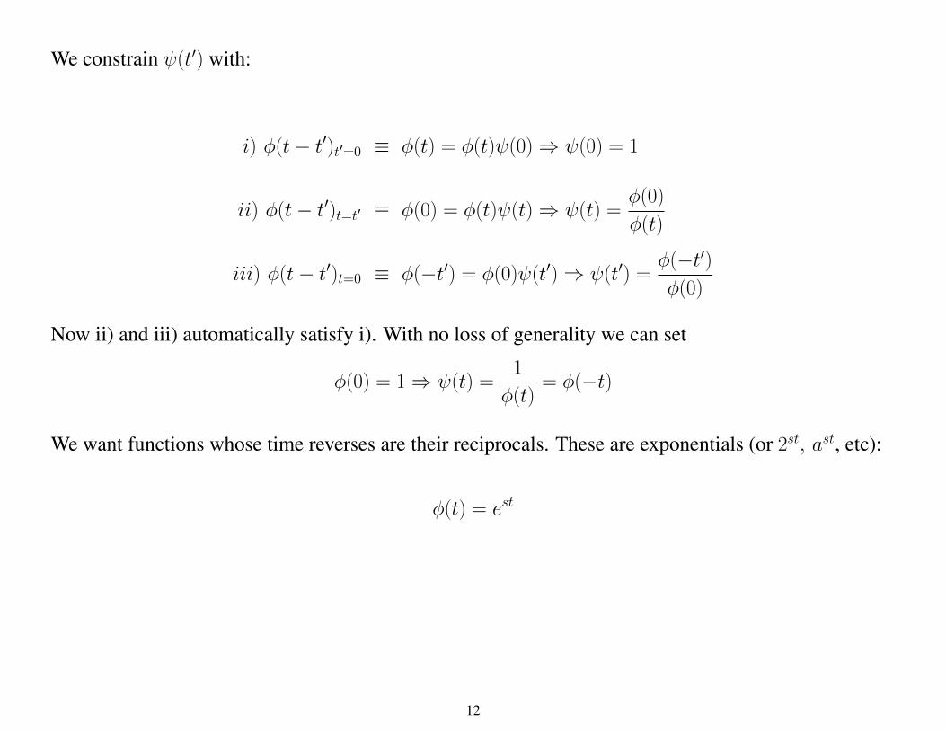
We constrain ψ(t�) with:

i) φ(t− t�)t�=0 ≡ φ(t) = φ(t)ψ(0) ⇒ ψ(0) = 1

ii) φ(t− t�)t=t� ≡ φ(0) = φ(t)ψ(t) ⇒ ψ(t) =

φ(0)

φ(t)

iii) φ(t− t�)t=0 ≡ φ(−t

�) = φ(0)ψ(t�) ⇒ ψ(t�) =

φ(−t�)

φ(0)

Now ii) and iii) automatically satisfy i). With no loss of generality we can set

φ(0) = 1 ⇒ ψ(t) =1

φ(t)= φ(−t)

We want functions whose time reverses are their reciprocals. These are exponentials (or 2st, ast, etc):

φ(t) = est

12

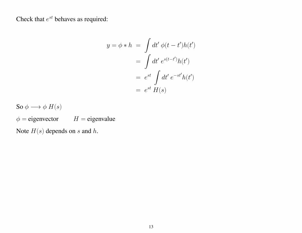
Check that est behaves as required:

y = φ ∗ h =

�dt

� φ(t− t�)h(t

�)

=

�dt

�es(t−t

�)h(t

�)

= est

�dt

�e−st

�h(t

�)

= estH(s)

So φ −→ φ H(s)

φ = eigenvector H = eigenvalue

Note H(s) depends on s and h.

13

Two kinds of systemsCausal

h(t) = 0 for t < 0

output now depends only on past values of input

H(s) =

� ∞

0dt

�e−st

�h(t

�) Laplace transform

Acausal

h(t) not necessarily 0 for t < 0

H(s) =

� ∞

−∞dt

�e−st

�h(t

�)|s=iω Fourier transform

Exponentials are useful for describing the action of a linear system because they “slide through” thesystem. If we can describe the actual input function in terms of exponential functions, then determiningthe resultant output becomes trivial. This is, of course, the essence of Fourier transform treatments oflinear systems and their underlying differential equations.

14

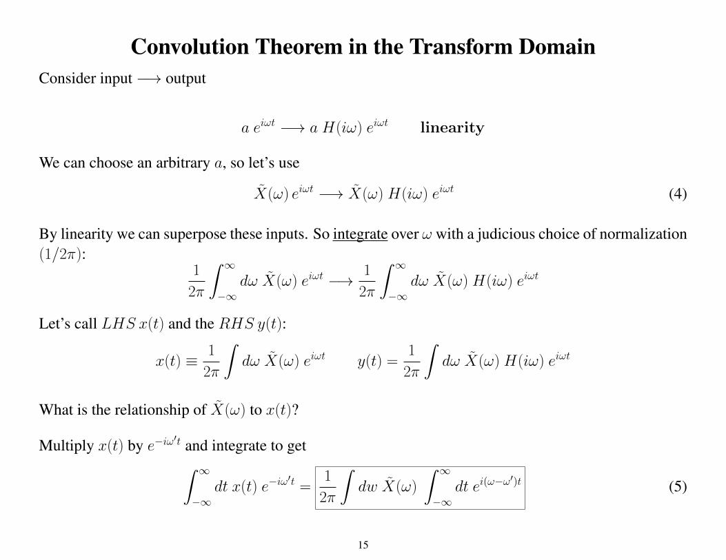
Convolution Theorem in the Transform DomainConsider input −→ output

a eiωt −→ a H(iω) eiωt linearity

We can choose an arbitrary a, so let’s use

X(ω) eiωt −→ X(ω) H(iω) eiωt (4)

By linearity we can superpose these inputs. So integrate over ω with a judicious choice of normalization(1/2π):

1

2π

� ∞

−∞dω X(ω) eiωt −→ 1

2π

� ∞

−∞dω X(ω) H(iω) eiωt

Let’s call LHS x(t) and the RHS y(t):

x(t) ≡ 1

2π

�dω X(ω) eiωt y(t) =

1

2π

�dω X(ω) H(iω) eiωt

What is the relationship of X(ω) to x(t)?

Multiply x(t) by e−iω�t and integrate to get

� ∞

−∞dt x(t) e

−iω�t=

1

2π

�dw X(ω)

� ∞

−∞dt e

i(ω−ω�)t (5)

15

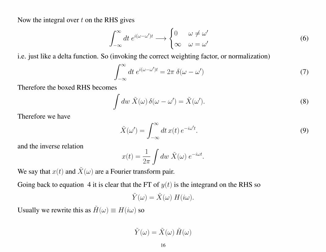
Now the integral over t on the RHS gives� ∞

−∞dt e

i(ω−ω�)t −→�0 ω �= ω�

∞ ω = ω� (6)

i.e. just like a delta function. So (invoking the correct weighting factor, or normalization)� ∞

−∞dt e

i(ω−ω�)t= 2π δ(ω − ω�

) (7)

Therefore the boxed RHS becomes�dw X(ω) δ(ω − ω�

) = X(ω�). (8)

Therefore we have

X(ω�) =

� ∞

−∞dt x(t) e

−iω�t. (9)

and the inverse relationx(t) =

1

2π

�dw X(ω) e−iωt

.

We say that x(t) and X(ω) are a Fourier transform pair.

Going back to equation 4 it is clear that the FT of y(t) is the integrand on the RHS so

Y (ω) = X(ω) H(iω).

Usually we rewrite this as H(ω) ≡ H(iω) so

Y (ω) = X(ω) H(ω)

16

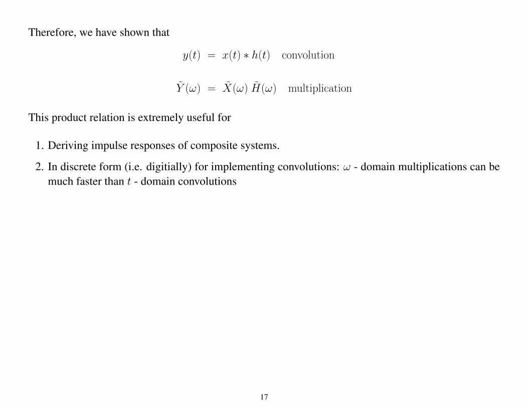
Therefore, we have shown that

y(t) = x(t) ∗ h(t) convolution

Y (ω) = X(ω) H(ω) multiplication

This product relation is extremely useful for

1. Deriving impulse responses of composite systems.

2. In discrete form (i.e. digitially) for implementing convolutions: ω - domain multiplications can bemuch faster than t - domain convolutions

17

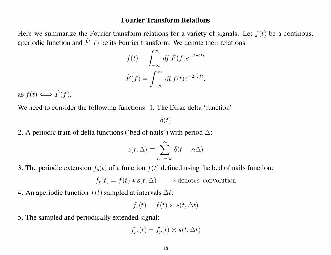
Fourier Transform Relations

Here we summarize the Fourier transform relations for a variety of signals. Let f (t) be a continous,aperiodic function and F (f ) be its Fourier transform. We denote their relations

f (t) =

� ∞

−∞df F (f )e

+2πift

F (f ) =

� ∞

−∞dt f (t)e

−2πift,

as f (t) ⇐⇒ F (f ).

We need to consider the following functions: 1. The Dirac delta ‘function’

δ(t)

2. A periodic train of delta functions (‘bed of nails’) with period ∆:

s(t,∆) ≡∞�

n=−∞δ(t− n∆)

3. The periodic extension fp(t) of a function f (t) defined using the bed of nails function:

fp(t) = f (t) ∗ s(t,∆) ∗ denotes convolution

4. An aperiodic function f (t) sampled at intervals ∆t:

fs(t) = f (t)× s(t,∆t)

5. The sampled and periodically extended signal:

fps(t) = fp(t)× s(t,∆t)

18

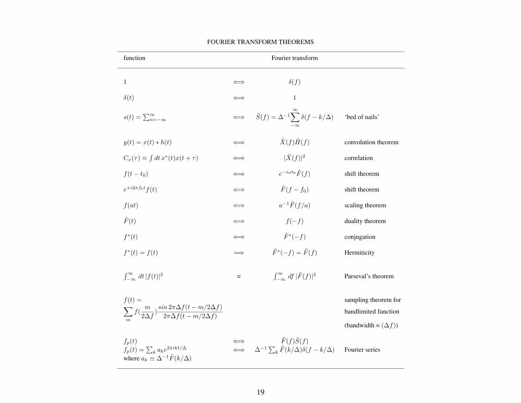
FOURIER TRANSFORM THEOREMS

function Fourier transform

1 ⇐⇒ δ(f)

δ(t) ⇐⇒ 1

s(t) =�∞

n=−∞ ⇐⇒ S(f) = ∆−1∞�

−∞δ(f − k/∆) ‘bed of nails’

y(t) = x(t) ∗ h(t) ⇐⇒ X(f)H(f) convolution theorem

Cx(τ) ≡�dt x

∗(t)x(t+ τ) ⇐⇒ |X(f)|2 correlation

f(t− t0) ⇐⇒ e−iωt0 F (f) shift theorem

e+i2πf0tf(t) ⇐⇒ F (f − f0) shift theorem

f(at) ⇐⇒ a−1

F (f/a) scaling theorem

F (t) ⇐⇒ f(−f) duality theorem

f∗(t) ⇐⇒ F

∗(−f) conjugation

f∗(t) = f(t) =⇒ F

∗(−f) = F (f) Hermiticity

�∞−∞ dt |f(t)|2 =

�∞−∞ df |F (f)|2 Parseval’s theorem

f(t) = sampling theorem for�

m

f(m

2∆f)sin 2π∆f(t−m/2∆f)

2π∆f(t−m/2∆f)bandlimited function

(bandwidth = (∆f))

fp(t) ⇐⇒ F (f)S(f)fp(t) =

�k ake

2πikt/∆ ⇐⇒ ∆−1�

k F (k/∆)δ(f − k/∆) Fourier serieswhere ak ≡ ∆−1

F (k/∆)

19

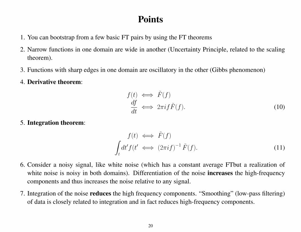
Points

1. You can bootstrap from a few basic FT pairs by using the FT theorems

2. Narrow functions in one domain are wide in another (Uncertainty Principle, related to the scalingtheorem).

3. Functions with sharp edges in one domain are oscillatory in the other (Gibbs phenomenon)

4. Derivative theorem:

f (t) ⇐⇒ F (f )

df

dt⇐⇒ 2πifF (f ). (10)

5. Integration theorem:

f (t) ⇐⇒ F (f )�

t

dt�f (t

� ⇐⇒ (2πif )−1F (f ). (11)

6. Consider a noisy signal, like white noise (which has a constant average FTbut a realization ofwhite noise is noisy in both domains). Differentiation of the noise increases the high-frequencycomponents and thus increases the noise relative to any signal.

7. Integration of the noise reduces the high frequency components. “Smoothing” (low-pass filtering)of data is closely related to integration and in fact reduces high-frequency components.

20

Gaussian FunctionsWhy useful and extraordinary?

1. We have the fundamental FT pair:

e−πt2 ⇐⇒ e

−πf2

This can be obtained using the FT definition and by completing the square. Once you know this FTpair, many situations can be analyzed without doing a single integral.

2. The Gaussian is one of the few functions whose shape is the same in both domains.

3. The width in the time domain (FWHM = full width at half maximum) is

∆t =2√ln 2√π

= 0.94

4. The width in the frequency domain ∆ν is the same.

5. Then

∆t∆ν =4ln 2

π= 0.88 ∼ 1.

6. Now consider a scaled version of the Gaussian function: Let t → t/T . The scaling theorem thensays that

e−π(t/T )2 ⇐⇒ Te

−π(fT )2.

The time-bandwidth product is the same as before since the scale factor T cancels. After all, ∆t∆νis dimensionless!

21

7. The Gaussian function has the smallest time-bandwidth product (minimum uncertainty wave packetin QM)

8. Central Limit Theorem: A quantity that is the sum of a large number of statistically independentquantities has a probability density function (PDF) that is a Gaussian function. We will state thistheorem more precisely when we consider probability definitions.

9. Information: The Gaussian function, as a PDF, has maximum entropy compared to any other PDF.This plays a role in development of so-called maximum entropy estimators.

22

Chirped SignalsConsider the chirped signal eiωt with ω = ω0 + αt, (a linear sweep in frequency). We write the signalas:

v(t) = eiωt

= ei(ω0t+αt2)

.

The name derives from the sound that a swept audio signal would make.

1. Usage or occurrence:

(a) wave propagation through dispersive media(b) objects that spiral in to an orbital companion, producing chirped gravitational waves(c) swept frequency spectrometers, radar systems(d) dedispersion applications (pulsar science)

2. We can use the convolution theorem to write

V (f ) = FT

�ei(ω0t+αt2)

�

= FT�eiω0t

�∗ FT

�ei(αt2)

�

= δ(f − f0) ∗ FT�ei(αt2)

�.

3. The FT pair for a Gaussian function would suggest that the following is true:

e−iπt2 ⇐⇒ e

−iπf2.

4. Demonstrate that this is true!

23

5. Within constants and scale factor, the FT of the chirped signal is therefore

V (f ) ∝ ei(π(f−f0)

2)

24

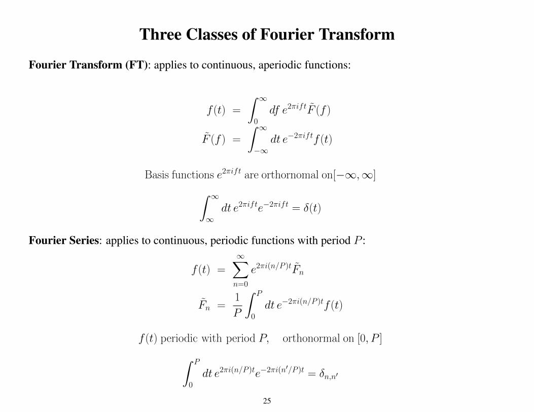
Three Classes of Fourier Transform

Fourier Transform (FT): applies to continuous, aperiodic functions:

f (t) =

� ∞

0df e

2πiftF (f )

F (f ) =

� ∞

−∞dt e

−2πiftf (t)

Basis functions e2πift

are orthornomal on[−∞,∞]

� ∞

∞dt e

2πifte−2πift

= δ(t)

Fourier Series: applies to continuous, periodic functions with period P :

f (t) =

∞�

n=0

e2πi(n/P )t

Fn

Fn =1

P

�P

0dt e

−2πi(n/P )tf (t)

f (t) periodic with period P, orthonormal on [0, P ]

�P

0dt e

2πi(n/P )te−2πi(n�/P )t

= δn,n�

25

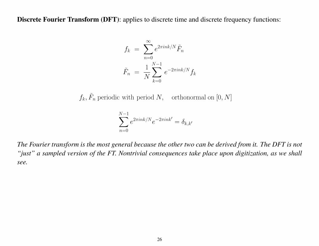
Discrete Fourier Transform (DFT): applies to discrete time and discrete frequency functions:

fk =

∞�

n=0

e2πink/N

Fn

Fn =1

N

N−1�

k=0

e−2πink/N

fk

fk, Fn periodic with period N, orthonormal on [0, N ]

N−1�

n=0

e2πink/N

e−2πink�

= δk,k�

The Fourier transform is the most general because the other two can be derived from it. The DFT is not“just” a sampled version of the FT. Nontrivial consequences take place upon digitization, as we shallsee.

26

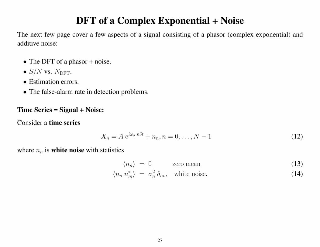
DFT of a Complex Exponential + NoiseThe next few page cover a few aspects of a signal consisting of a phasor (complex exponential) andadditive noise:

• The DFT of a phasor + noise.• S/N vs. NDFT.• Estimation errors.• The false-alarm rate in detection problems.

Time Series = Signal + Noise:

Consider a time series

Xn = A eiωo nδt

+ nn, n = 0, . . . , N − 1 (12)

where nn is white noise with statistics

�nn� = 0 zero mean (13)�nn n

∗m� = σ2

nδnm white noise. (14)

27

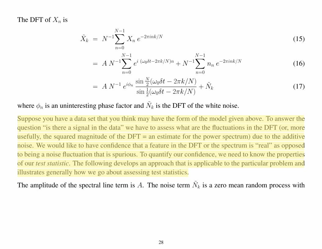
The DFT of Xn is

Xk = N−1

N−1�

n=0

Xn e−2πink/N (15)

= A N−1

N−1�

n=0

ei (ω0δt−2πk/N)n

+N−1

N−1�

n=0

nn e−2πink/N (16)

= A N−1

eiφn

sinN

2 (ω0δt− 2πk/N)

sin12(ω0δt− 2πk/N)

+ Nk (17)

where φn is an uninteresting phase factor and Nk is the DFT of the white noise.

Suppose you have a data set that you think may have the form of the model given above. To answer thequestion “is there a signal in the data” we have to assess what are the fluctuations in the DFT (or, moreusefully, the squared magnitude of the DFT = an estimate for the power spectrum) due to the additivenoise. We would like to have confidence that a feature in the DFT or the spectrum is “real” as opposedto being a noise fluctuation that is spurious. To quantify our confidence, we need to know the propertiesof our test statistic. The following develops an approach that is applicable to the particular problem andillustrates generally how we go about assessing test statistics.

The amplitude of the spectral line term is A. The noise term Nk is a zero mean random process with

28

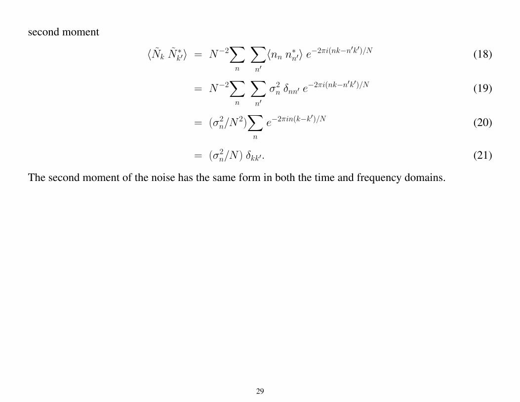
second moment

�Nk N∗k�� = N

−2�

n

�

n�

�nn n∗n�� e−2πi(nk−n

�k�)/N (18)

= N−2�

n

�

n�

σ2nδnn� e

−2πi(nk−n�k�)/N (19)

= (σ2n/N

2)

�

n

e−2πin(k−k

�)/N (20)

= (σ2n/N) δkk�. (21)

The second moment of the noise has the same form in both the time and frequency domains.

29

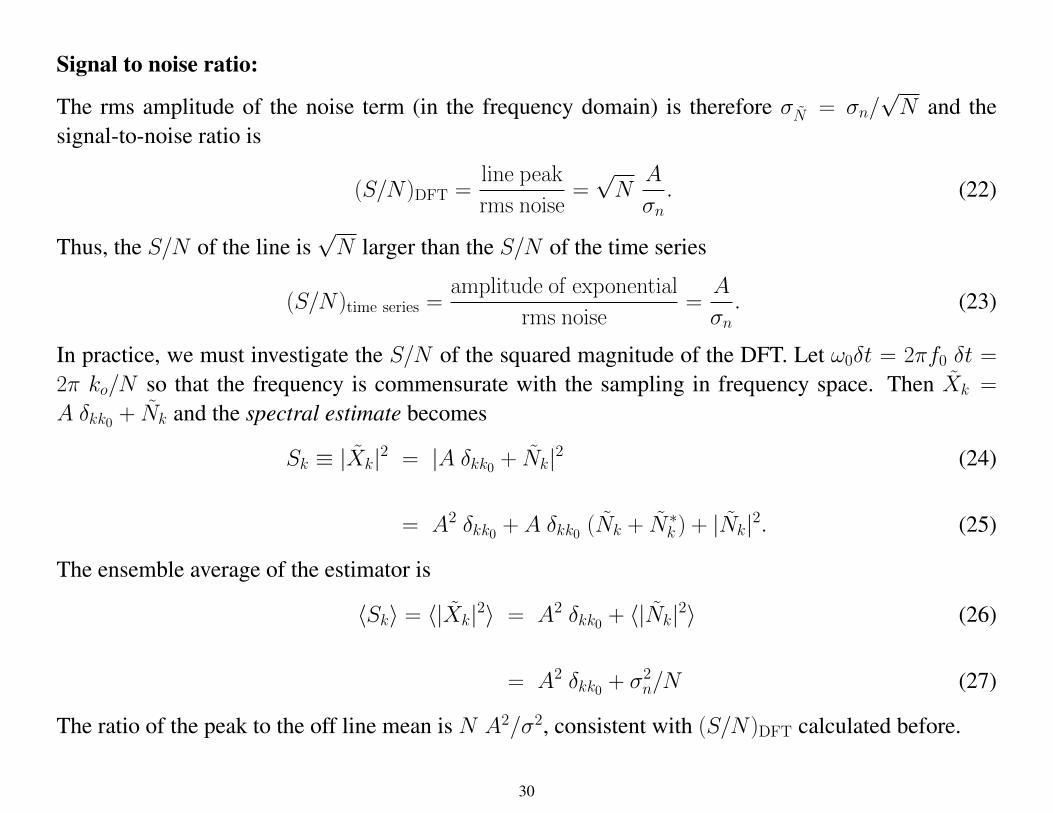
Signal to noise ratio:

The rms amplitude of the noise term (in the frequency domain) is therefore σN

= σn/√N and the

signal-to-noise ratio is

(S/N)DFT =line peak

rms noise=

√N

A

σn. (22)

Thus, the S/N of the line is√N larger than the S/N of the time series

(S/N)time series =amplitude of exponential

rms noise=

A

σn. (23)

In practice, we must investigate the S/N of the squared magnitude of the DFT. Let ω0δt = 2πf0 δt =2π ko/N so that the frequency is commensurate with the sampling in frequency space. Then Xk =

A δkk0 + Nk and the spectral estimate becomes

Sk ≡ |Xk|2 = |A δkk0 + Nk|2 (24)

= A2 δkk0 + A δkk0 (Nk + N

∗k) + |Nk|2. (25)

The ensemble average of the estimator is

�Sk� = �|Xk|2� = A2 δkk0 + �|Nk|2� (26)

= A2 δkk0 + σ2

n/N (27)

The ratio of the peak to the off line mean is N A2/σ2, consistent with (S/N)DFT calculated before.

30

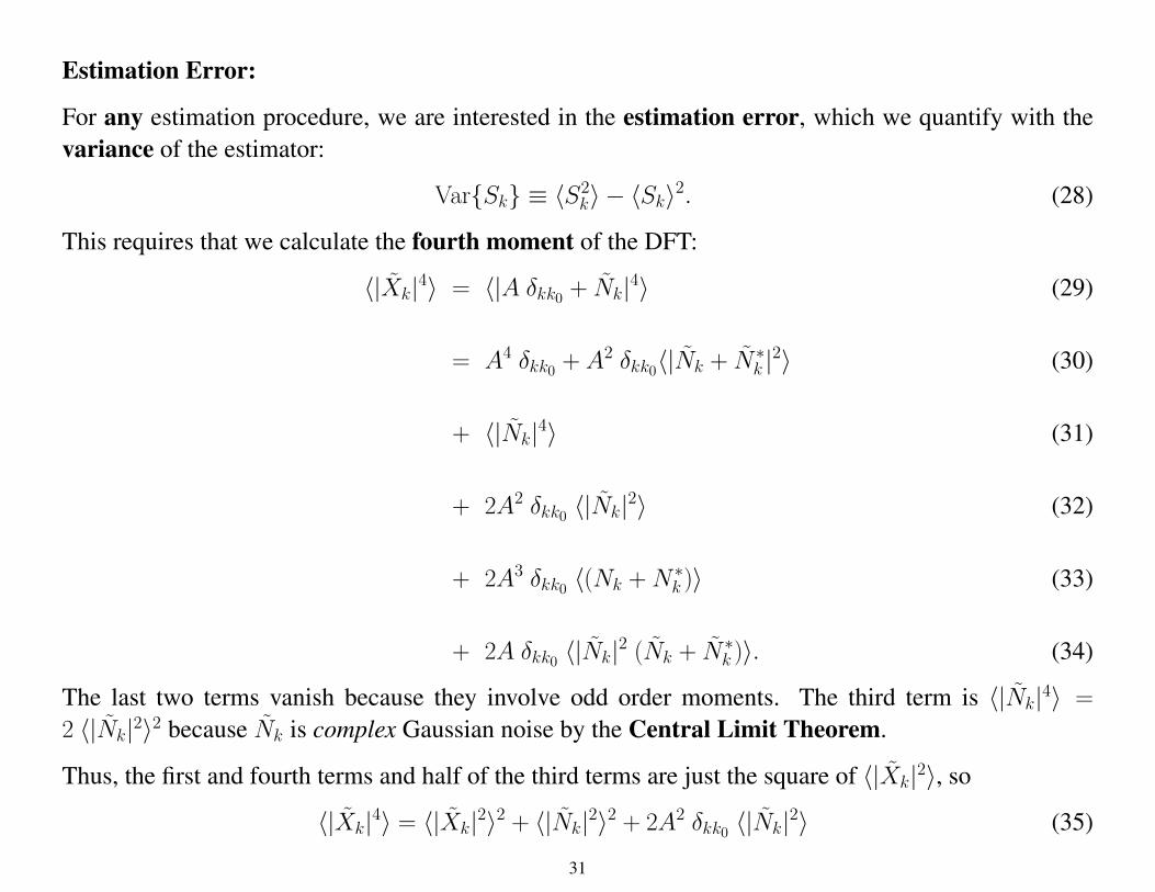
Estimation Error:

For any estimation procedure, we are interested in the estimation error, which we quantify with thevariance of the estimator:

Var{Sk} ≡ �S2k� − �Sk�2. (28)

This requires that we calculate the fourth moment of the DFT:

�|Xk|4� = �|A δkk0 + Nk|4� (29)

= A4 δkk0 + A

2 δkk0�|Nk + N∗k|2� (30)

+ �|Nk|4� (31)

+ 2A2 δkk0 �|Nk|2� (32)

+ 2A3 δkk0 �(Nk +N

∗k)� (33)

+ 2A δkk0 �|Nk|2 (Nk + N∗k)�. (34)

The last two terms vanish because they involve odd order moments. The third term is �|Nk|4� =

2 �|Nk|2�2 because Nk is complex Gaussian noise by the Central Limit Theorem.

Thus, the first and fourth terms and half of the third terms are just the square of �|Xk|2�, so

�|Xk|4� = �|Xk|2�2 + �|Nk|2�2 + 2A2 δkk0 �|Nk|2� (35)

31

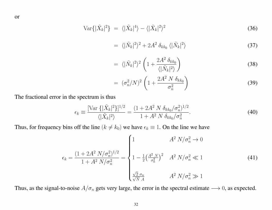
or

Var{|Xk|2} = �|Xk|4� − �|Xk|2�2 (36)

= �|Nk|2�2 + 2A2 δkk0 �|Nk|2� (37)

= �|Nk|2�2�1 +

2A2 δkk0

�|Nk|2�

�(38)

= (σ2n/N)

2

�1 +

2A2N δkk0σ2n

�(39)

The fractional error in the spectrum is thus

�k ≡[Var {|Xk|2}]1/2

�|Xk|2�=

(1 + 2A2N δkk0/σ

2n)1/2

1 + A2 N δkk0/σ2n

. (40)

Thus, for frequency bins off the line (k �= k0) we have �k ≡ 1. On the line we have

�k =(1 + 2A

2N/σ2

n)1/2

1 + A2 N/σ2n

=

1 A2N/σ2

n→ 0

1− 12

�A2N

σ2n

�2A

2N/σ2

n� 1

√2 σn√N A

A2N/σ2

n� 1

(41)

Thus, as the signal-to-noise A/σn gets very large, the error in the spectral estimate −→ 0, as expected.

32

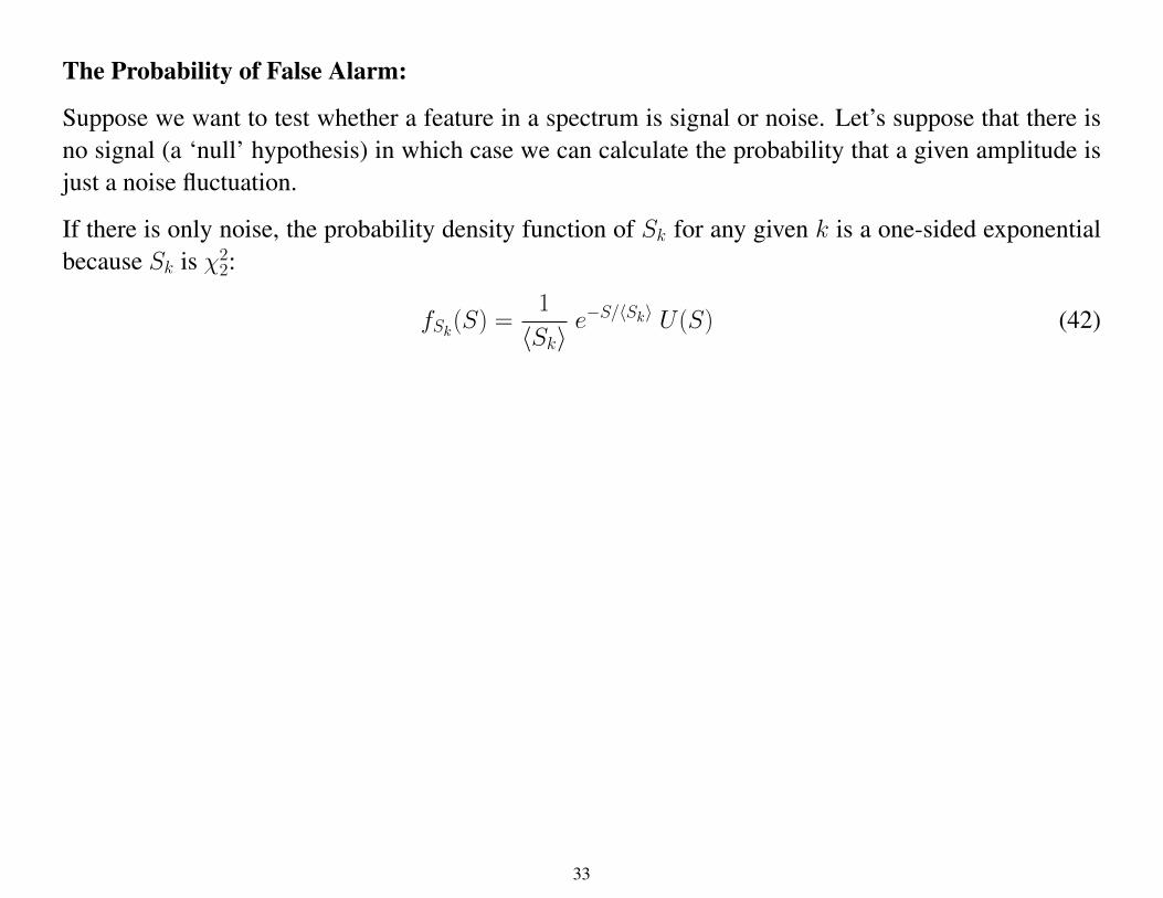
The Probability of False Alarm:

Suppose we want to test whether a feature in a spectrum is signal or noise. Let’s suppose that there isno signal (a ‘null’ hypothesis) in which case we can calculate the probability that a given amplitude isjust a noise fluctuation.

If there is only noise, the probability density function of Sk for any given k is a one-sided exponentialbecause Sk is χ2

2:

fSk(S) =1

�Sk�e−S/�Sk� U(S) (42)

33

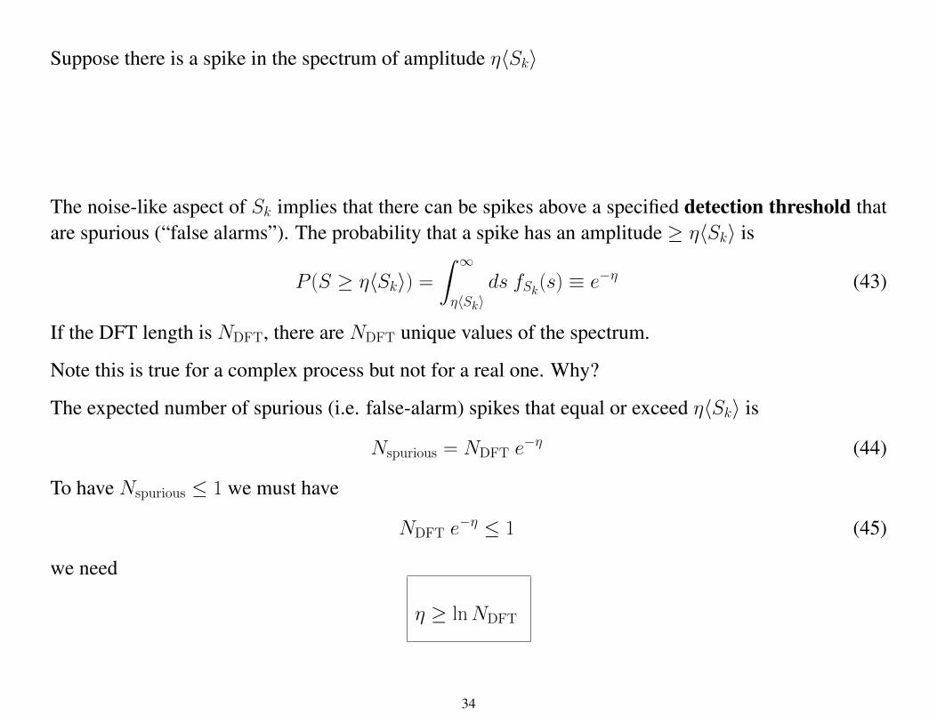
Suppose there is a spike in the spectrum of amplitude η�Sk�

The noise-like aspect of Sk implies that there can be spikes above a specified detection threshold thatare spurious (“false alarms”). The probability that a spike has an amplitude ≥ η�Sk� is

P (S ≥ η�Sk�) =� ∞

η�Sk�ds fSk(s) ≡ e

−η (43)

If the DFT length is NDFT, there are NDFT unique values of the spectrum.

Note this is true for a complex process but not for a real one. Why?

The expected number of spurious (i.e. false-alarm) spikes that equal or exceed η�Sk� is

Nspurious = NDFT e−η (44)

To have Nspurious ≤ 1 we must have

NDFT e−η ≤ 1 (45)

we need

η ≥ lnNDFT

34

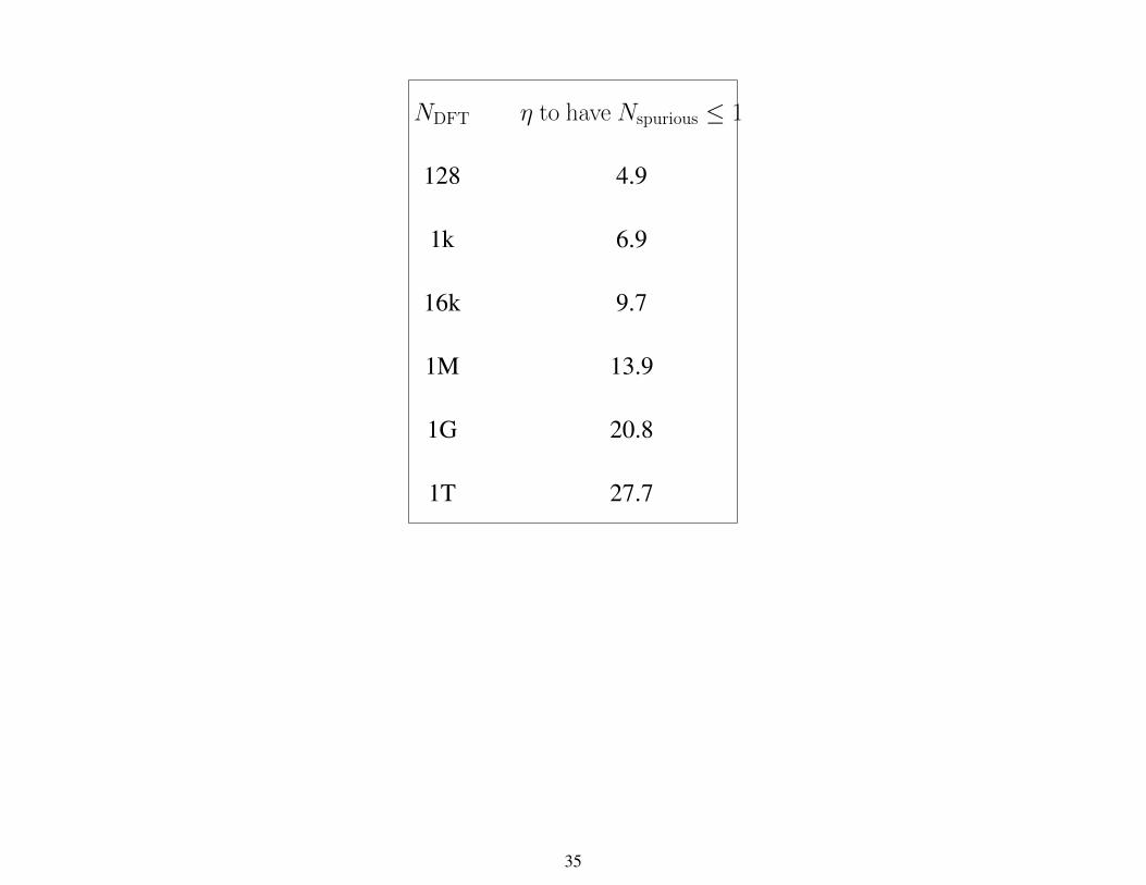
NDFT η to have Nspurious ≤ 1

128 4.9

1k 6.9

16k 9.7

1M 13.9

1G 20.8

1T 27.7

35