Embed Size (px)
Citation preview
UNLV Retrospective Theses & Dissertations
1-1-2000
A Web-based finite element model for heat transfer A Web-based finite element model for heat transfer
Trevor Allen Wilcox University of Nevada, Las Vegas
Follow this and additional works at: https://digitalscholarship.unlv.edu/rtds
Repository Citation Repository Citation Wilcox, Trevor Allen, "A Web-based finite element model for heat transfer" (2000). UNLV Retrospective Theses & Dissertations. 1230. http://dx.doi.org/10.25669/gs0h-eph2
This Thesis is protected by copyright and/or related rights. It has been brought to you by Digital Scholarship@UNLV with permission from the rights-holder(s). You are free to use this Thesis in any way that is permitted by the copyright and related rights legislation that applies to your use. For other uses you need to obtain permission from the rights-holder(s) directly, unless additional rights are indicated by a Creative Commons license in the record and/or on the work itself. This Thesis has been accepted for inclusion in UNLV Retrospective Theses & Dissertations by an authorized administrator of Digital Scholarship@UNLV. For more information, please contact [email protected].
INFORMATION TO USERS
This manuscript has been reproduced from the microfilm master. UMI films the text directly from the original or copy submitted. Thus, some thesis and dissertation copies are in typewriter face, while others may be from any type of computer printer.
The quality of this reproduction is dependen t upon the quality of the copy subm itted. Broken or indistinct print, colored or poor quality illustrations and photographs, print bleedthrough, substandard margins, and improper alignment can adversely affect reproduction.
In the unlikely event that the author did not send UMI a complete manuscript and there are missing pages, these will be noted. Also, if unauthorized copyright material had to be removed, a note will indicate the deletion.
Oversize materials (e.g., maps, drawings, charts) are reproduced by sectioning the original, beginning at the upper left-hand comer and continuing from left to right in equal sections with small overlaps.
Photographs included in th:e original manuscript have been reproduced xerographically in this copy. Higher quality 6” x 9” black and white photographic prints are available for any photographs or illustrations appearing in this copy for an additional charge. Contact UMI directly to order.
Bell & Howell Information and Learning 300 North Zeeb Road, Ann Artror, Ml 48106-1346 USA
800-521-0600
UMI
Reproduced with permission of the copyright owner. Further reproduction prohibited without permission.

Reproduced with permission of the copyright owner. Further reproduction prohibited without permission.

NOTE TO USERS
Page(s) missing in number only; text follows. Page(s) weremicrofilmed as received.
39
This reproduction is the best copy available
UMI’
Reproduced with permission of the copyright owner. Further reproduction prohibited without permission.

Reproduced with permission of the copyright owner. Further reproduction prohibited without permission.

A WEB-BASED FINITE ELEMENT MODEL FOR HEAT TRANSFER
by
Trevor A. Wilcox
Bachelor of Science in Mathematics University of Alaska, Anchorage
1997
Master of Science in Mathematics University of Nevada, Las Vegas
1998
A thesis submitted in partial fulfillment of the requirements for the
Master of Science Degree Department of Mechanical Engineering
Howard R. Hughes College of Engineering
Graduate College University of Nevada, Las Vegas
December 2000
Reproduced with permission of the copyright owner. Further reproduction prohibited without permission.

UMI Number: 1403103
UMJUMI Microform 1403103
Copyright 2001 by Beil & Howell information and Learning Company. All rights reserved. This microform edition is protected against
unauthorized copying under Title 17, United States Code.
Bell & Howell Information and Learning Company 300 North Zeeb Road
P.O. Box 1346 Ann Arbor, Ml 48106-1346
Reproduced with permission of the copyright owner. Further reproduction prohibited without permission.

IJNTV Thesis ApprovalThe Graduate College University o f Nevada, Las Vegas
September 22 .20 00
The Thesis prepared by
T r e v o r A l l e n W ilc o x
Entitled
A Web Based Finite Element Model for Heat Transfer
is approved in partial fulfillment o f the requirements for the degree of
M a ste r s o f S c ie n c e
tee Member
Examinanon Committee Member
Examination Committee Chair
Dean o f the Graduate College
Graduate College Faculty Representative
PR/1017-53/1.00 11
Reproduced with permission of the copyright owner. Further reproduction prohibited without permission.

ABSTRACT
A Web-Based Finite Element Model for Heat Transfer
by
Trevor A. Wilcox
Dr. Darrell Pepper, Examination Committee Chair Professor and Chairman, Department of Mechanical Engineering
University of Nevada, Las Vegas
A web based Java program has been developed to solve 2-D transient or steady state
heat transfer problems. The numerical solver is based on the finite element method. The
program is designed to work with both triangle and quadrilateral elements. In this thesis
the development of the finite element method, using the Galerkin weighted residuals
method, is reviewed and the technique applied to the advection-diffusion equation for the
transport of temperature. The Java code and graphical interface used to implement the
solver for use on the Internet is discussed.
ui
Reproduced with permission of the copyright owner. Further reproduction prohibited without permission.

TABLE O F CONTENTS
ABSTRACT................................................. iü
LIST OF FIGURES..................................................................................................................vi
LIST OF TABLES..................................... ............................................................................. vii
ACKNOWLEDGEMENTS...................... - .......................................................................... vüi
CHAPTER 1 ................................................ 1Introduction............................................... 1
CHAPTER 2 ................................................ 1Heat Equation............................................ 1Conduction Problem................................. 4Finite Difference M ethod........................ 6Finite Volume M ethod............................ 15Boundary Element M ethod..................... 17Boundary Fitted Coordinates.................. - ........................................................................... 22
CHAPTERS................................................ 27Finite Element Method............................. 27Galerkin Formulation............................... 28Elements.................................................... 31
CHAPTER 4 ................................................ 40Java History................................................- ........................................................................... 40Applet......................................................... 41Abstract Window Toolkit........................ 43Swing.......................................................... - ........................................................................... 44Java — Fortran Comparison..................... 45Finite Element Program .......................... 49
CHAPTERS................................................ 51Numerical Results..................................... - ........................................................................... 51
CHAPTER 6 ................................................ 71Conclusion................................................. 71
IV
Reproduced with permission of the copyright owner. Further reproduction prohibited without permission.

APPENDICES.................................................................................................. 73Notation.................................................................................................................................. 73Analytic Solution................................................................................................................... 74U nits........................................................................................................................................81Program Screen Shot of Tab One........................................................................................82Program Screen Shot o f Tab Tw o.......................................................................................83Program Screen Shot of Tab Three.....................................................................................84Gauss Points for Triangular Elements................................................................................ 85Gauss Points for Quadrilateral Elements........................................................................... 86GUI How Chart......................................................................................................................87Solver How C hart................................................................................................................. 88Sample Input Data File......................................................................................................... 91
BIBLIOGRAPHY................................................................................................................... 93
VITA........................................................................................................................................... 95
Reproduced with permission of the copyright owner. Further reproduction prohibited without permission.
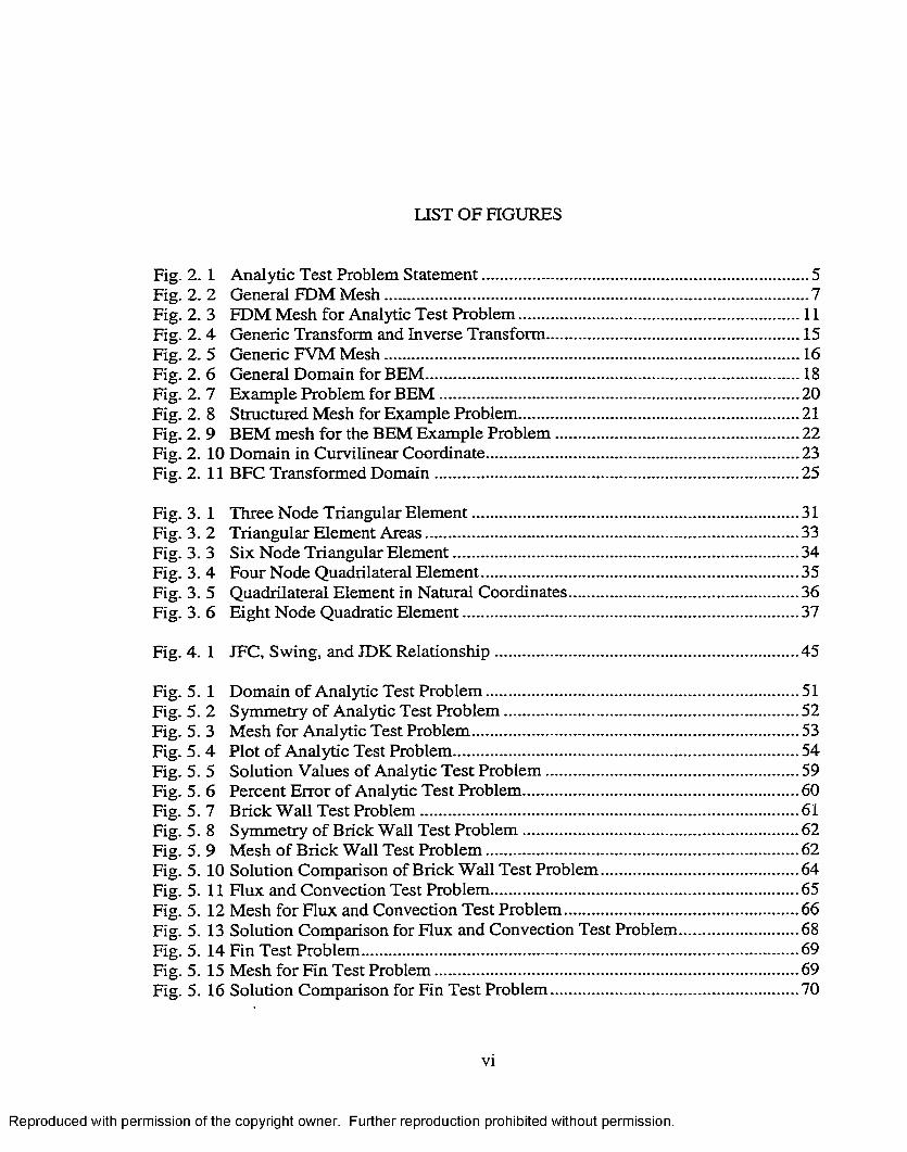
LIST OF FIGURES
Fig. 2. I Analytic Test Problem Statement............................................................................5Fig. 2. 2 General FDM M esh..................................................................................................7Fig. 2. 3 FDM Mesh for Analytic Test Problem................................................................. 11Fig. 2 .4 Generic Transform and Inverse Transform...........................................................15Fig. 2. 5 Generic FVM M esh................................................................................................ 16Fig. 2. 6 General Domain for BEM.......................................................................................18Fig. 2. 7 Example Problem for B E M ................................................................................... 20Fig. 2. 8 Structured Mesh for Example Problem................................................................. 21Fig. 2. 9 BEM mesh for the BEM Example Problem........................................................ 22Fig. 2. 10 Domain in Curvilinear Coordinate........................................................................ 23Fig. 2. 11 BFC Transformed Domain.................................................................................... 25
Fig. 3. 1 Three Node Triangular Element............................................................................31Fig. 3. 2 Triangular Element Areas...................................................................................... 33Fig. 3. 3 Six Node Triangular Element................................................................................ 34Fig. 3. 4 Four Node Quadrilateral Element..........................................................................35Fig. 3. 5 Quadrilateral Element in Natural Coordinates..................................................... 36Fig. 3. 6 Eight Node Quadratic Element..............................................................................37
Fig. 4. 1 JFC, Swing, and JDK Relationship...................................................................... 45
Fig. 5. 1 Domain of Analytic Test Problem........................................................................ 51Fig. 5. 2 Symmetry of Analytic Test Problem.................................................................... 52Fig. 5. 3 Mesh for Analytic Test Problem............................................................................53Fig. 5. 4 Plot of Analytic Test Problem................................................................................ 54Fig. 5. 5 Solution Values of Analytic Test Problem...........................................................59Fig. 5. 6 Percent Error of Analytic Test Problem................................................................60Fig. 5. 7 Brick Wall Test Problem........................................................................................61Fig. 5. 8 Symmetry of Brick Wall Test Problem ................................................................62Fig. 5. 9 Mesh of Brick Wall Test Problem........................................................................ 62Fig. 5. 10 Solution Comparison of Brick Wall Test Problem..............................................64Fig. 5. 11 Flux and Convection Test Problem....................................................................... 65Fig. 5. 12 Mesh for Flux and Convection Test Problem...................................................... 66Fig. 5. 13 Solution Comparison for Flux and Convection Test Problem............................68Fig. 5. 14 Fin Test Problem..................................................................................................... 69Fig. 5. 15 Mesh for Fin Test Problem.................................................................................... 69Fig. 5. 16 Solution Comparison for Fin Test Problem......................................................... 70
VI
Reproduced with permission of the copyright owner. Further reproduction prohibited without permission.

LIST OF TABLES
Table 5 .1 Solution Comparison of Analytic Test Problem.............................................55Table 5. 2 3 Node Solution of Analytic Test Problem......................................................55Table 5. 3 4 Node Solution of Analytic Test Problem......................................................56Table 5 .4 6 Node Solution of Analytic Test Problem......................................................56Table 5. 5 8 Node Solution of Analytic Test Problem......................................................57Table 5. 6 EDM Solution of Analytic Test Problem......................................................... 57Table 5. 7 Percent Error Comparison of Analytic Test Problem.....................................58Table 5. 8 Solution Comparison of Brick Wall Test Problem.........................................63Table 5 .9 Solution Comparison for Flux and Convection Test Problem.......................67Table 5. 10 Solution Comparison for Fin Test Problem.....................................................70
vu
Reproduced with permission of the copyright owner. Further reproduction prohibited without permission.

ACKNOWLEDGEMENTS
I would Like to express my most sincere thanks to Dr. Darrell W. Pepper for his
guidance and constant interest. Without his supervision, I would have not been able to
complete this thesis.
Also, I would like to thank the committee members. Dr. Mohamed Trabia, Dr. Yi-
Tung Chen, and Dr. Laxmi Gewali, for their interest and assistance.
Furthermore, I would like to thank my parents, Rena Offlitt and David Wilcox, for
their continuing support in my education.
Thanks also to the many who have helped me throughout my quest for higher
education.
vm
Reproduced with permission of the copyright owner. Further reproduction prohibited without permission.

CHAPTER 1
Introduction
For the purpose of this thesis we will concentrate on a unique numerical scheme for
the solution of heat transfer in two dimensions. We first look at the equation for heat
conduction in a general domain
^ - v ( K v r ) = G
For simple domains solutions to the conduction problem can be found in most heat
transfer books or can be solved analytically. As the geometry or physics of the problem
becomes more complex, the problem becomes more difficult or impossible to solve using
exact methods. Since most practical problems of interest involve complex domains and
boundary conditions, one must look to numerical methods to solve the problem.
The concept of present day finite elements dates back to the 1940’s. It wasn’t until
the 1970’s when an influx of contributions from other fields enlarged the types of
problems being solved (Comini et al., 1994). Since the 1970’s the finite element method
has evolved into a powerful solver for solid mechanics, fluid mechanics, and heat
transfer. We will employ the finite element method to solve the heat transfer problem in
this thesis.
Reproduced with permission of the copyright owner. Further reproduction prohibited without permission.
Before we develop the finite element method, we will first give a survey of other
numerical methods and compare them to the finite element. Two of the most popular
numerical methods are the finite difference and finite volume methods. The finite
difference and finite volume approaches are fairly versatile and relatively easy to
implement on regular domains. However, both methods become troublesome to
implement when the domains are irregular. However, the finite element method works
well for regular as well as irregular geometry.
To solve the general heat equation, a finite element program has been developed in
the Java programming language. Java was created by Sun Microsystems engineers in
1996. Java is an object oriented programming language similar to C++. The reason for
choosing Java is because it was designed, in part, to be deployed over the Internet. The
purpose of this work was to develop a finite element program that is available over the
Internet. The solver consists of standard techniques used in the finite element method.
The graphical user interface makes use of Java’s Swing components. These Swing
components allow the user to do preprocessing by viewing the mesh before the problem
is solved. After the problem is solved the solution is displayed for the user.
The finite element program solves heat transfer problems involving conduction with
convection. The user must establish the mesh for the domain using either triangles or
quadrilateral elements. The program can solve regular and irregular domains with a
variety of boundary conditions. As the program exists, aU information about the problem
to be solved must be stored in a data file. A sample data file can be found in the
appendices.
Reproduced with permission of the copyright owner. Further reproduction prohibited without permission.

CHAPTER2
Heat Equation
The general, two-dimensional time dependent energy equation in Cartesian
coordinates can be written as (Incropera and DeWitt, 1996)
r a r a r a r^~\~U “h V a a4"——dx dx dx ' a%_ dy _ 3y_
or, in vector notation.
P c .a rdt
W T = V[KVT] + G
The governing equation we will discuss for illustrating development of the finite element
procedure is the Poisson equation form (steady state) for diffusion (i.e., conduction) of
heat. The form of the governing equation is
-V (K V r) = (2 (2-1)
where Q is a heat source or sink and K is the thermal conductivity. There are three types
of boundary conditions associated with equation (2. 1). The first is the Dirichlet
condition given by
r = T fixed
The second type of boundary condition is the Neumann, written as
Reproduced with permission of the copyright owner. Further reproduction prohibited without permission.

where q is the heat flow. The last type of boundary condition is the mixed, or Robin,
which is normally associated with convection. For convection, the boundary condition is
q = h { T - T . )
where 7^ is the ambient temperature. In order to solve the heat equation appropriate
boundary, initial conditions, and time dependency need to be specified. These boundary
conditions are stated in mathematical from based on the physical make up of the problem
at hand. A general boundary condition form for (2. 1) can be described as
a T + b ^ + c = 0 (2.2)an
Equation (2. 2) gives Neumann (flux) condition when a = 0 , mixed (Robin) condition if
a 5 0 and , and if 6 = 0 we have Dirichlet condition. The solution of the Poisson
equation is dependent upon the type of boundary condition associated with the problem.
In the next section we will look at a simple conduction problem.
Conduction Problem
A conduction problem with Dirichlet conditions will first be solved using the method
of separation of variables. Using the method of separation of variables requires a
relatively simple geometry (Myers, 1998). To use the method of separation of variables
the partial differential equation must be linear and homogeneous. Also, the boundary
conditions must be linear and partially homogeneous. For these reasons we have chosen
the problem shown in Fig. 2. 1 with constant AT.
Reproduced with permission of the copyright owner. Further reproduction prohibited without permission.

Ai .
^ ( 0 , y ) = 0 #
riT '^ ( X ,0 ) = 0
L-► X
Fig. 2. 1 Analytic Test Problem Statement
ATV^r + Q = 0
f ( 0 . , ) = 0
T {L ,y )= T ,
^ ( x , 0 ) = 0
T (x ,L )= T ,
Te satisfy the necessary homogeneity assume the solution is of the following form
(2.3)
(2.4)
(2.5)
(2.6)
(2.7)
Reproduced with permission of the copyright owner. Further reproduction prohibited without permission.
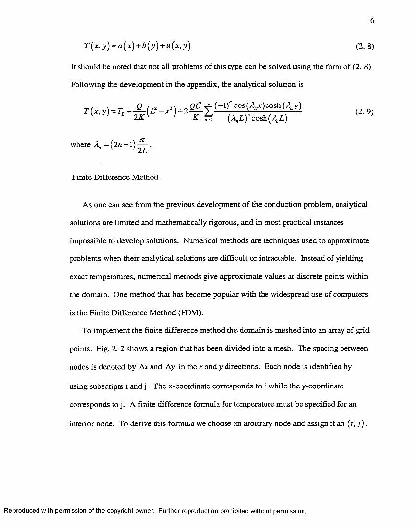
T{x,y)=^a{x) + b{y)-\-u{x,y) (2.8)
It should be noted that not all problems of this type can be solved using the form of (2. 8).
Following the development in the appendix, the analytical solution is
where = (2 n —l ) - ^ . ' 2L
Finite Difference Method
As one can see from the previous development of the conduction problem, analytical
solutions are limited and mathematically rigorous, and in most practical instances
impossible to develop solutions. Numerical methods are techniques used to approximate
problems when their analytical solutions are difficult or intractable. Instead of yielding
exact temperatures, numerical methods give approximate values at discrete points within
the domain. One method that has become popular with the widespread use of computers
is the Finite Difference Method (FDM).
To implement the finite difference method the domain is meshed into an array of grid
points. Fig. 2. 2 shows a region that has been divided into a mesh. The spacing between
nodes is denoted by Ax and Ay in the x and y directions. Each node is identified by
using subscripts i and j. The x-coordinate corresponds to i while the y-coordinate
corresponds to j. A finite difference formula for temperature must be specified for an
interior node. To derive this formula we choose an arbitrary node and assign it an (f, j ) .
Reproduced with permission of the copyright owner. Further reproduction prohibited without permission.

The node to the left and the right of (i, j ) are assigned —1, / ) and (/+, y ) . Likewise,
the nodes above and below ( / , / ) are assigned ( / ,y + l) and (f ,y —1).
i + 1 , 1 + 1
Fig. 2. 2 General FDM Mesh
Before we derive the formulas for the finite difference method we should review
some background material. Recall the Taylor series expansion of the function / (x)
f { x + h ) = f { x ) + f ' { x ) h + ^ - ^ h ^ + - - -2 !
Truncating the series after two terms we have the approximation
Reproduced with permission of the copyright owner. Further reproduction prohibited without permission.

(2. 10)
The expression given by (2. 10) is called the forward difference. The backward
difference is obtained by replacing h by -h in (2. 10) and is given by
(2. 11)
Subtracting (2. 11) from (2. 10) we obtain the central difference approximation
/'W=^[/(^+^)-/(^-^)]
By retaining another term in the Taylor series, this type of analysis can be extended to
derive the central difference approximation fo r / ''(x ) as
This analysis can be extended to partial derivatives giving
(x, y) = - ^ [ r ( x + / i , y ) -2 T (x , y )+ r ( x - f t , y)]
T ^ { x , y ) = ^ \ T { x , y + k ) - T { x , y - k ) \
T „ { x , y ) = ^ \ T { x , y + k ) - 2 T { x , y ) ^ T { x , y - k ) \
It is convenient to express the above equations in the following notation
T(^<y)=T,.,
T (x+ h ,y )= T „ ^ j
Reproduced with permission of the copyright owner. Further reproduction prohibited without permission.

T { x -h ,y ) ^ T ^ _ , j
T {x ,y + k)=T^j^,
T { x ,y -k )= T i j_ ,
Thus, rewrite the partial derivatives as
T=(x,y) = ^ 2 (i;.!,; - ) (2. 12)
(^+i.j "*■ -1.1 ) (2- 13)
where A and k have been replaced with Ax and Ay . To solve the heat conduction
problem we replace the partial derivatives in T^+Tyy = —— with (2. 12) and (2. 13).K
Doing this and taking Ax = Ay = S we have
i+U +^.y+i (2. 14)
Here, Tj y is a solution to an interior node. This interior node we have just analyzed is
one of many, perhaps hundreds or thousands of nodes in a 2-D region. To solve for the
temperature of every node in a domain, a separate finite difference equation must be
derived for each node. These nodal equations make up a system of equations that have as
many unknowns as the number of equations.
Reproduced with permission of the copyright owner. Further reproduction prohibited without permission.

10
For illustrative purposes we will look at the same problem we solved analytically
earlier. The problem is restated here and shown in Fig. 2. 1.
(2. 15)
(2.16)
T ( L , y ) = T , (2 . 1 7 )
(2.18)
T{x ,L )= T^ (2.19)
We will divided the arbitrary domain into a 5x5 grid with equal spacing as shown in Fig.
2 .3 .
Reproduced with permission of the copyright owner. Further reproduction prohibited without permission.

1 ___________
1 2 3 4
Fig. 2. 3 FDM Mesh for Analytic Test Problem
11
Next, we write a single linear equation of the form (2. 14) for each of the nine interior
grid points.
~2i2 “ 32 “ 23 ~ 21 + ~ ‘ K
-T22 -T 42 -T|3 -T 31 +47^2 -
- 52 “ 32 ~^43 “ 41 +4^42
25:
f o25:
■^13 ~ ^3 3 ~ ^ 2 4 ~ ^ 2 2 + ^ ^ 2 3 ~ 25:
Reproduced with permission of the copyright owner. Further reproduction prohibited without permission.

12
-? 4 3 “ ^2 3 “ ^ 3 4 - ^ 2 + ^ ^ 3
-7^ -7^3 -Tlz +^^3
~ ^ 3 4 “ ^1 4 “ ^ 2 5 “ ^2 3
-T^ -T ^ -T js - 7 3 + 47^
f g25:
f GK
f GK
f GK
“ 54 “ 34 - ^ 5 ~^43 +4T^
This system of equations can be solved by Gaussian elimination. There are 45
coefficients and since u is known at the boundary points we move these 12 terms to the
right hand side. After moving the terms we have 33 nonzero interior coefficients out of
81 in a 9x9 system. To show the sparse structure of the system of equation we will now
write the system in matrix form.
A T = b
Using natural ordering for the unknowns we have
T = [T22,7^2’^ 2 ’^ » ^ 3 ’^ 3 ’^ ’^ ’^ ]
The coefficient matrix is
Reproduced with permission of the copyright owner. Further reproduction prohibited without permission.

13
A =
4 -1 0 - I 0 0 0 0 0- I 4 - I 0 - I 0 0 0 00 -1 4 - I 0 -1 0 0 0
-1 0 - I 4 -1 0 - I 0 00 -1 0 - I 4 - I 0 -1 00 0 -1 0 -1 4 - I 0 - I0 0 0 - I 0 -1 4 -1 00 0 0 0 - I 0 -1 4 -10 0 0 0 0 -1 0 -1 4
b =
and the right hand side is
Kf g
K
Ê lü .K
Kf g
Kf g
Kf g
Kf g
Kf g. .
Because the equations are similar in form, iterative methods can be use to solve the
sparse system. One such solver is the Gauss-Seidel method (Gerald, 1978). Solvers and
complete programs for solving finite difference problems can be found on the web and in
the literature. Thus,
Reproduced with permission of the copyright owner. Further reproduction prohibited without permission.

14
1— — ----^ ---- LLJ-+— = o (2.20)
In implementing the finite difference method we discretized the region using a set of
regularly spaced nodes. The spacing in the x-direction is uniform and equal to the
spacing in the y-direction, which gives a square pattern for the nodal points. A
rectangular pattern can also be easily implemented. However, using non-square patterns
makes the problem considerably more difficult. Since non-orthogonal meshes are
prohibitive it can be difficult to create a mesh for a domain that is not orthogonal. For
irregular domains the boundary of the region can be approximated as closely as possible
using an orthogonal mesh. Where the mesh does not fall on the boundary the boundary
conditions must be incorporated into the surrounding nodes. In some cases the domain
may be transformed from the geometric domain into the computational domain, see Fig.
2. 4. As shown in Fig. 2. 4, 9Jt denotes the forward transform and [371] denotes the
inverse transform. Once in computational space the problem is easily solved by the
computer. The biggest difficulty with transforming a domain into computational space is
deriving the transform and inverse transforms.
Reproduced with permission of the copyright owner. Further reproduction prohibited without permission.

15
[971]-^
Fig. 2. 4 Generic Transform and Inverse Transform
Finite Volume Method
The next numerical method we will look at is the Finite Volume Method (FVM). The
finite volume method is based on the conservation of a physical property such as thermal
energy. Thus the finite volume method always starts with an integral conservation
formulation. First, the governing conservation principle is stated in integral form. The
integral form of the steady state heat equation over a fixed volume is
[v~ T d V + J^-^dV = 0 (2. 21)
OUsing the mean value theorem of integrals the integral over — can be evaluated. AlsoK
the volume integral over can be transformed to a surface integral by applying the
divergence theorem (Ozi§ik, 1993).
Reproduced with permission of the copyright owner. Further reproduction prohibited without permission.

16
f V T - n d S + V — J s K
where
WT-n 3 rdn
Here V denotes a small control volume
Similar to the finite difference method, the domain is subdivided into a regular mesh
using non-overlapping control volumes. However, the node locations are located at the
centers of each grid instead of at the intersections as seen in Fig. 2. 5
#i -1,1+1
ei , j - 1 i + 1 , j \
ei -1,1
ei. j
ei+ 1 .j
ei - 1 ,1 -1
•i. j + 1
•i+ 1 .j-1
Fig. 2. 5 Generic FVM Mesh
Reproduced with permission of the copyright owner. Further reproduction prohibited without permission.

17
The space between each grid line is denoted by Ax and Ay . Each grid line makes up a
control volume face, which lies midway between each node at (z± l/2 ,y ) and
( i ,y ± l /2 ) .
Once the control volumes are defined, we can apply the conservation statement to a
typical control volume. After applying equation (2. 21) to the {i ,j ) control volume we
have
0 = - f ^ d y - ! ^ d x + l %dxdyX - U 2 Jy-1/2 .*+1/2 Jj+l /2 0 y JûxAy
Here we assign unit depth, so the integrals are evaluated over the volumes AxAy ( l ) .
Using simple finite difference expressions, the heat balance on the control volume can be
written as
+ Ax+-^AxAy = 0Ax Ay Ax Ay K
Dividing by AxAy and rearranging we get
T . . U + r 0 (2.22)Ax" Ay' itxAyK ^
which looks Uke the finite difference expression, equation (2. 20). Equation (2. 22) can
be solved in a similar manner to the finite difference method.
Boundary Element Method
The Boundary Element Method (BEM) is now being used as an alternative to the
finite element method (Brebbia and Dominguez, 1989) for simple problem definitions.
Studies have found that the BEM can yield accurate results on problems that involve
Reproduced with permission of the copyright owner. Further reproduction prohibited without permission.

18
stress and fracture analysis. The BEM is also being used for domains that are infinite or
where rapid prototyping is being used. When using boundary elements only the surface
of the domain needs to be meshed. The method allows for easier mesh regeneration in
the event that the geometry of the problem changes. Although it should be noted that in
its ease of use one must be careful when developing codes, as the BEM is prone to
numerical errors (Brebbia and Dominguez, 1989).
To illustrate the BEM we will again use Poisson’s form of the heat equation given by
V Y = - —K
and defined over the domain Q with boundary T . A generic domain can be seen in Fig.
2.6
Fig. 2. 6 General Domain for BEM
The boundary conditions are of two types: the ‘essential’ type T on Fj and the ‘natural’
type — on F j (Brebbia and Dominguez, 1989). The boundary is given by F = Fj + F j . dn
Let
Reproduced with permission of the copyright owner. Further reproduction prohibited without permission.

19
T - T ^ O
dT dT dn dn
# 0
— dTbe the residuals where T and —— are approximations. Take W to be an arbitrarydn
weighting function with derivatives on the boundary given by
dWdn
The governing equation in integral form is
QK
WdQ. dTI dn dn
w d T - f (r-r)-^dr•*'1 ' ' dn
Integrating equation (2. 23) by parts once yields
dT dW dT dW Q dx dx dy dy K
W d a = - f ^ W d T - L ^ W d T dn dn
(2. 23)
- [ T ^ d T + { T ^ d T • 1 dn dn
Integration by parts again gives
l ^ W d T
+ [ T ^ d T + [ f ^ d T • 2 on on
(2. 24)
Equation (2. 24) is the basic statement for the boundary element formulation of Poisson’s
form of the heat equation. By passing the unknowns to the left hand side one can write
(Brebbia and Dominguez, 1989)
KT = F
Reproduced with permission of the copyright owner. Further reproduction prohibited without permission.

20
where T is a vector of the unknowns.
The elements used in the boundary element method are s im ile to elements used in
the finite element method. These elements include linear, bilinear, quadratic, and
biquadratic. To illustrate the difference in meshes between the FD M and BEM, consider
the domain shown in Fig. 2. 7.
T = T,
r = T
Fig. 2. 7 Example Problem for BEM
A structured mesh is shown in Fig. 2. 8.
Reproduced with permission of the copyright owner. Further reproduction prohibited without permission.
21
5 11■■■a
>
17 23 1 • •
, ,4 .
p . . %
,iO , 16 22 :■II I
) 5 ,
, ,2 -
. V ■
,s'- ,20 ,,
28
27
26
.25
24
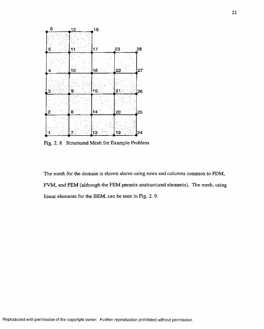
Fig. 2. 8 Structured Mesh for Example Problem
The mesh for the domain is shown above using rows and columns common to FDM,
FVM, and FEM (although the FEM permits unstructured elements). The mesh, using
linear elements for the BEM, can be seen in Fig. 2. 9.
Reproduced with permission of the copyright owner. Further reproduction prohibited without permission.

22
10 11
V 12
13
18 17
14
15
Fig. 2. 9 BEM mesh for the BEM Example Problem
The mesh for the BEM uses considerable less nodes than that of the FDM, FVM, or even
the FEM. The interesting feature to notice is the absence of interior nodes — the BEM has
transformed the solution integral from an area to a Hne, i.e. a I-D problem. As one can
imagine, there are considerable savings on the number of nodes and element for large
domains. The accuracy of the BEM is as good as the FEM, and in some cases may
provide the only solution.
Boundary Fitted Coordinates
To overcome some of the problems of irregular geometries one can use the method of
boundary fitted coordinates (BFC). The method consists of transforming irregular
Reproduced with permission of the copyright owner. Further reproduction prohibited without permission.

23
geometries into a rectangular computational domain. The computational domain may be
composed of rectangular sub-domains. One begins by using a curvilinear coordinate
system to create the mesh of the domain. The mesh should be smooth and a sufficiently
fine grid should be used in areas where the solution has large variations.
To provide a foundation for the boundary fitted coordinate method we will look at a
transformation of an annular ring domain in cylindrical coordinates (Thompson et al,
1985). In this case the curvilinear coordinate system is taken to be r and 6 . The
annular region and coordinate orientation can be seen in Fig. 2. 10.
Fig. 2. 10 Domain in Curvilinear Coordinate
Reproduced with permission of the copyright owner. Further reproduction prohibited without permission.

24
The well known relationship between the curvilinear coordinates and the Cartesian
coordinates is given by
x(^r,û) = r c o s 0
y (r ,û ) = r s in0
The inverse transform is then defined as
r{x ,y ) = ylx^ + y^
0 { x , y ) = tan\ x y
Using the transform we can represent the annular ring as a rectangle. However, for the
purpose of programming it is convenient to normalize the region. To normalize the
curvilinear coordinates to an interval of [O, l ] , we introduce the coordinates ^ and 77 .
The relationship between the two coordinate systems is defined as
7 7 = -
or
Û{^)=27T^
r (7 ) = ri+(r2-ri)77
The transform can be rewritten as
= cos (2tz-#)
7) = ('i + ('*2 - ) ??) sin (2;< )
Reproduced with permission of the copyright owner. Further reproduction prohibited without permission.

25
where 0 < < 1 and Q<r]<l. The transformed domain is shown in Fig. 2.11
Fig. 2.11 BFC Transformed Domain
The relationship of interior grid points between the computational space and the physical
domain can be expressed as
ax '0 (2.25)
with appropriate boundary conditions. Equations (2. 25) and (2. 26) are in physical
space, the corresponding equations in computational space are (Fletcher, 1991)
(2. 26)
Reproduced with permission of the copyright owner. Further reproduction prohibited without permission.

d<^ ~ d ^ T j drj-
26
(2. 27)
(2. 28)
where
a =r fdxvâ7y
+v3%/
g _ dx dx By dy ^ d ^dr j d^dr)
^ = [ ÿ ] 4 &)Once the boundary conditions are known in the computational domain, equations (2. 27)
and (2. 28) can be solved using simple finite difference techniques. The concept of
boundary fitted coordinates can be extended to 3-D regions of any shape. Although this
method can be used on almost any geometry, it may be very difficult to derive the
transform and its inverse.
Reproduced with permission of the copyright owner. Further reproduction prohibited without permission.

CHAPTERS
Finite Element Method
The finite element method (FEM) is similar to the finite difference scheme in that it
uses numerical approximation to provide solutions to physical problems. The finite
element method dates back to the 1940’s and the 1950’s. However, there is general
agreement that the term “finite element method” actually appeared in a paper by Clough
in 1960 (Pepper and Heinrich, 1992). This is also the time when digital computers were
starting to be used to solve matrix type problems. The early use of finite elements was
aimed at problems of structural analysis. Starting in the 1970’s the use of finite elements
for non-structural problems began in earnest.
The governing equation we will be using for illustrating the finite element method is
the Poisson equation for heat conduction with an internal source,
V Y = — (3.1)K
We now look to formulate the “weak statement” for this problem using the method of
weighted residuals (MWR). Greens theorem is implemented to reduce the problem from
second order to first order over the domain. To apply the MWR the domain must be
discretized into elements. For each of these elements the temperature will be
approximated by using known functions Af,-(x,y). The functions V-(x, y) are called
27
Reproduced with permission of the copyright owner. Further reproduction prohibited without permission.

28
shape functions. We can approximate the temperature distribution using the trial
approximation
(3.2)1=1
where n is the number of nodes in the element. We will use the Galerkin form of the
MWR to formulate the finite element method. In general, when using equation (3. 2) to
approximate the left hand side of equation (3. 1) a true solution is not achieved. The best
we can hope for is a “residual” function representing the error of the approximation. Let
the error for the heat conduction problem with constant conductivity be
R{T,x,) = - K V ^ T - Q
Here T is an approximation to the analytical solution and cannot be made to equal the true
solution unless the error vanishes over the whole domain. Since the error cannot be made
to go to zero, we seek to minimize the error. To minimize the error we multiply by a
weighting function and force the integral to vanish as given by
|^W ;.R(r,x,)riQ = 0
Galerkin Formulation
Now we will formulate the Galerkin weighted residual by setting the weight equal to
the interpolating function. As before, let
K
be defined over the domain Q with boundary T . We will use the MWR as described
earlier (dropping subscript i for simplicity)
Reproduced with permission of the copyright owner. Further reproduction prohibited without permission.
29
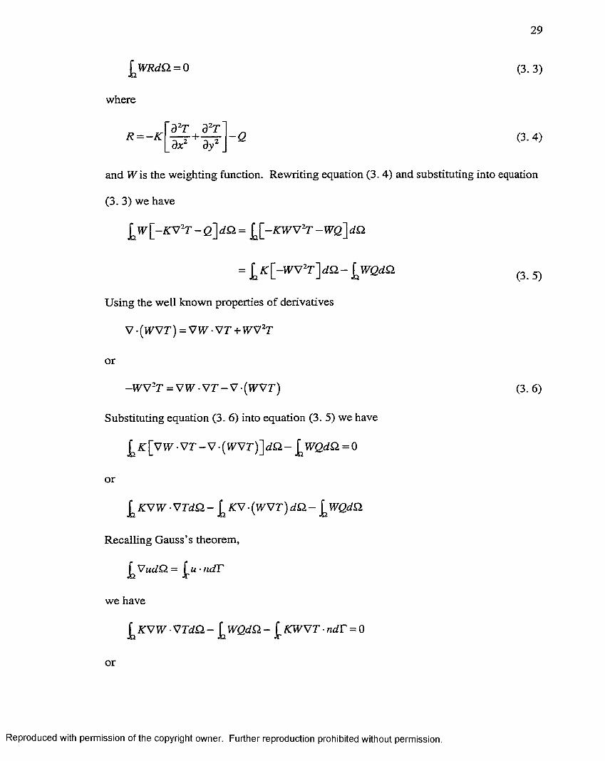
£ w R d a = 0 (3.3)
where
R = - K a 'T ^ a ' r- 2 (3.4)
gkc' ity'
and Wis the weighting function. Rewriting equation (3. 4) and substituting into equation
(3. 3) we have
^ W \ - K V " - T - 0 \ d Q . = - W Q \ d a
= l K [ - w v ^ ] d a - \ w Q d a (3 , 3 )
Using the well known properties of derivatives
V • (wvr) = vw ■ VT+wv'r
or
-WW-T = V W - V T - V - { W V T ) (3.6)
Substituting equation (3. 6) into equation (3. 5) we have
£ K [v w • vr - V • ( wvr)] da - [wQdO.=o
or
£ w • V T d a - £ - [w v t ] d a - ^ w Q d a
Recalling Gauss’s theorem,
V u d a =_[.“ ■
we have
£ K V W WTda - ^ W Q d a - K W V T ■ ndT = 0
or
Reproduced with permission of the copyright owner. Further reproduction prohibited without permission.

30
^ K [ V W ■ V T ) - W Q ] d a + l w ^ K ^ ^ d T = Q (3.7)
We now approximate the temperature over the domain using the trial approximation
defined by equation (3. 2). For the Galerkin formulation we set . Thus equation
(3.7) is
1 ^ 1'dN, dNj dN, dNj
dx dx d y d yd a T, = l N , Q d a - l N , [ K ^ ' ^ a r p . s )
Equation (3. 8) can be expressed in matrix notation as
K r = F
where
d a
and
V = [ f , ] = ] ^ N , Q d a - l N , ^ d T
where
The K matrix is commonly called the stiffness matrix while F is called the load vector
(Pepper and Heinrich. 1992). If advection is present, the matrix form can be expressed as
(U + K ) r = F
where
dN , . dN j
Reproduced with permission of the copyright owner. Further reproduction prohibited without permission.

31
The functions u and v have been interpolated using the shape functions, and summation
is implied by the index k .
Elements
The fixst type of element we will discus is the three node triangular element.
Although there are different ways to number the nodes, the general practice is to number
the nodes of an element in the counterclockwise order (Pepper and Heinrich, 1992). We
will denote the node locations as shown in Fig. 3 .1 .
y
XFig. 3. 1 Three Node Triangular Element
The linear triangular element is represented by the following polynomial
Y = cc +a2X + cXjy
Reproduced with permission of the copyright owner. Further reproduction prohibited without permission.

32
The linear shape functions for the triangular element in x and y coordinates are
N,=-^{x2y^-x2y2)+[y.-y^)x-t{x2-x2)y']
^2 + - 7 i ) ^ + ( 4 - ^ ) y ]
^3 = ^ [ ( ^ y 2 - ^ y i ) + ( > 'l - y 2 ) ^ + ( j ^ - ^ ) 3 ']
where
^=~[(^y2 -^yi)+{^yi - 4 7 3 )+(^2^3 - ^ ^ 2 )]
For computational purposes it is convenient to rewrite the shape functions into a natural
coordinate system. The natural coordinate variables are defined as
* = T
where A^, and Aj are the areas as shown in Fig. 3. 2. The coordinates x and y are
related to the coordinates ^ a n d ^ by
^ = ^l^+^2^2+^3^
Reproduced with permission of the copyright owner. Further reproduction prohibited without permission.

33
1
2
Fig. 3 .2 Triangular Element Areas
The shape functions in the natural coordinate system are defined as
^1=^1
^3 =^3
The derivatives of the shape function can be calculated using the chain rule.
The quadratic triangular element is made up of six nodes as shown in Fig. 3.3. The
polynomial representing the six node triangle is an extension of the linear interpolating
polynomial and is given by
Y = a^+ a^_x+ 0 ,7 + + a^xy -^a^y'
Reproduced with permission of the copyright owner. Further reproduction prohibited without permission.

34
y
X
Fig. 3. 3 Six Node Triangular Element
The shape functions in the natural coordinate system are given by
^ 2 = 6 ( 2 6 - 1 )
^5 =4^1 A
^6 —4 ^ A
The derivatives for the shape functions are calculated in the same manner as those for the
linear triangle.
Reproduced with permission of the copyright owner. Further reproduction prohibited without permission.

35
The second type of element commonly used in the finite element method is the
quadrilateral. The quadrilateral element is a four sided polygon usually consisting of
four, eight, or nine nodes. Typically the higher the order of the element the more
accurate the results, but such elements consume substantially more computational
resources. We will discus the four and eight node elements.
The four node quadrilateral element and node numbering are shown in Fig. 3 .4
y
X
Fig. 3. 4 Four Node Quadrilateral Element
The interpolating polynomial for the four node element is given by
y = <%; -^-a^x-k-a^y-^a^xy
Using the relation given by
Reproduced with permission of the copyright owner. Further reproduction prohibited without permission.

36
X = X N i + X2^2 -I- ^ 3 +
y = yi i+ yzNo + + y^N^
the element can be transformed into the natural coordinate system as shown in Fig. 3. 5
(Pepper and Heinrich, 1992). Hence,
A r .= i ( i - f ) ( l+ ) 7 )
where —1 < ^ < 1 and - ! < ? ; < 1 .
Fig. 3. 5 Quadrilateral Element in Natural Coordinates
Reproduced with permission of the copyright owner. Further reproduction prohibited without permission.

37
The calculation of the derivative is analogous to the triangular element.
The eight node quadratic element and node numbering are shown in Fig. 3. 6 .
y
X
Fig. 3. 6 Eight Node Quadratic Element
The shape functions for the eight node quadratic are as follows:
N, =-
N^ =2
Reproduced with permission of the copyright owner. Further reproduction prohibited without permission.

38
4
( l - r ) ( l + # )2
y _ (H -^ )( l + 77)(^+77-l)4
2
^ . { l -^ ) { l+ T ] ){ l+ ^ -r i )’ 4
^ . ( l - ^ ' ) ( l - ^ )® 2
where —1 < ^ < 1 and -1 < 7 < 1. Again, the calculation of the derivatives is similar to
that of the triangular element.
Reproduced with permission of the copyright owner. Further reproduction prohibited without permission.

NOTE TO USERS
Page(s) missing in number only; text follows. Page(s) weremicrofilmed as received.
39
This reproduction is the best copy available
UMI*
Reproduced with permission of the copyright owner. Further reproduction prohibited without permission.

CHAPTER 4
Java History
Java stems from Sun Microsystems engineers Patrick Naughton and James Gosling
who wanted to develop a language that could be used for consumer electronics in 1991.
The language was needed to generate compact code that would run on different central
processing units (CPUs) with little memory. This project was dubbed the “Green”
Project (Horstmann, 1999). The Green project engineers designed a portable language
that uses intermediate code that is interpreted by a virtual machine. This code could run
on any hardware that had the proper interpreter. Since the code is machine independent a
programmer can be confident that a program developed in Java will run on any hardware
or platform, provided it has the correct interpreter.
Sun Microsystems first release of Java was in 1996. The release was followed by
Java 1.02a shortly after the initial release. It was found that these versions of Java were
not able to produce serious applications. The first major revision was Java 1.1. Although
Java 1.1 was a major step in the right direction, it was the release of Java 1.2 that
provided the means to produce sophisticated code. Release 1.2 provided a wealth of new
components. These components allow for greater flexibility in programming Applets.
40
Reproduced with permission of the copyright owner. Further reproduction prohibited without permission.

41
Applet
Java programs that run on the web are called applets. Byte-codes are downloaded
form the Internet and then run on the clients system. For an applet to work the user must
have a Java-enabled web browser to interpret the byte-codes. Applets provide a versatile
way to present programs and data across the Internet. Applets can be used to add active
content to web pages. Also, applets can be used to convey pseudo-applications. A
pseudo-applications is an applet that looks and feels like a stand-alone application, but
does not have the functionality of an application.
There are some drawbacks to using applets. For example, downloading applets
over a dial-up connection may be very slow. Also, problems can arise when web
browsers do not run the most current version of Java. Sun, the creators of Java, have
provided a solution to the problem called a Java Plug-in. Java Plug-in is software that
allows the programmer to direct applets on their web pages to run Sun’s Java Runtime
Environment (JRE) instead of the web browsers default Java virtual machine. The
current release provides support for Microsoft Internet Explorer and Netscape Navigator
on various Win32 platforms. There is also support for Compaq Tru64™ Unix(r), Linux,
and HPUX. Work is under way to support other platforms.
Using the following HTML tag one can automatically force the browser to download
the correct Java Plug-in if it is not currently installed on the system viewing the applet.
This ensures that a client will be able to correctly view the applet. To use Java Plug-in in
IE on Windows 95, Windows 98 or Windows NT 4.0, use the OBJECT tag. The following
is an example of mapping an APPLET tag to a Java Plug-in tag:
Original APPLET tag:
Reproduced with permission of the copyright owner. Further reproduction prohibited without permission.

42
<APPLET c o d e = " H e a t X f e r . c l a s s " c o d e b a s e = " h . t m l / " a l i g n = " b a s e l i n e " w i d t h = " 2 0 0 " h e i g h t = " 2 0 0 " ><PARAM NAM E="m odel" V A L T J E = " m o d e l s /H e a t X f e r .x y z " >N o J a v a 2 SDK, S t a n d a r d E d i t i o n v 1 . 3 s u p p o r t f o r A P P L E T 'i </A P P L E T >
N ew OBJECT tag:
<OBJECT c l a s s i d = " c l s i d : 8 A D 9 C 8 4 0 - 0 4 4 E - l l D l - B 3 E 9 - 0 0 8 0 5 F 4 9 9 D 9 3 "w i d t h = " 2 0 0 " h e i g h t = " 2 00" a l i g n = " b a s e l i n e "c o d e b a s e = " h t t p : / / J a v a . s u n . c o m / p r o d u c t s / p l u g i n / 1 . 3 / j i n s t a l l - 1 3 -W in 3 2 . c a b # V e r s i o n = l , 3 , 0 , 0 " ><PARAM NAM E="code" VALUE=" H e a t X f e r . c l a s s "><PARAM N A M E = " c o d e b a se " V A L U E = " h tm l /"><PARAM N A M E ="type" VALUE="a p p l i c a t i o n / x - J a v a - a p p l e t ; v e r s i o n = l . 3 "><PARAM NAME= " m o d e l" VALUE= " m o d e l s / m o d e l s / H e a t X f e r . x y z " > <PARAM N A M E = " s c r i p t a b l e " VALUE="t r u e ">N o J a v a 2 SDK, S t a n d a r d E d i t i o n v 1 . 3 s u p p o r t f o r APPLET I! </O BJEC T>
To use Java Plug-in in Netscape Navigator 3 or 4 on Windows 95, Windows 98,
Windows N T 4.0, or Solaris operating environments, use the EMBED tag. The following
example maps an APPLET tag to a Java Plug-in EMBED tag:
Original APPLET tag:
<AlPPLET c o d e = " H e a t X f e r . c l a s s " c o d e b a s e = "h t m l /" a l i g n = "b a s e l i n e " w i d t h = " 2 0 0 " h e i g h t = " 2 0 0 " ><PARAM NAME= " m o d e l " VALUE= " m o d e l s / m o d e l s / H e a t X f e r . x y z " >N o J a v a 2 SDK, S t a n d a r d E d i t i o n v 1 . 3 s u p p o r t f o r A P P L E T !! </A P P L E T >
N ew EMBED tag:
< EMBED t y p e = "a p p l i c a t i o n / x - J a v a - a p p l e t ; v e r s i o n = l .3 " w i d t h = " 200"h e i g h t = " 2 0 0 " a l i g n = " b a s e l i n e " c o d e = " H e a t X f e r . c l a s s " c o d e b a s e = " h t m l / " m o d e l = " m o d e l s / m o d e l s / H e a t X f e r . x y z " p l u g i n s p a g e = "h t t p : / / J a v a . s u n . c o m / p r o d u c t s / p l u g i n / 1 . 3 / p l u g i n - i n s t a l l . h t m l ">
Reproduced with permission of the copyright owner. Further reproduction prohibited without permission.
43
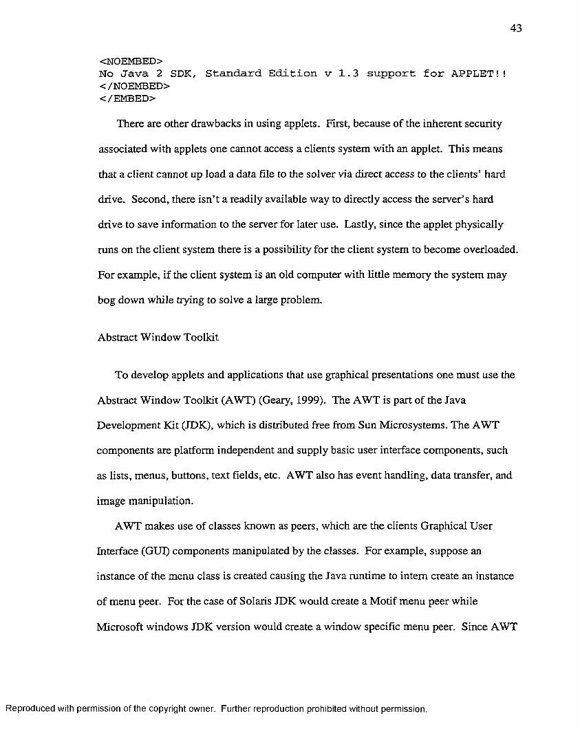
<NOEMBED>N o J a v a 2 SDK, S t a n d a r d E d i t i o n v 1 . 3 s u p p o r t f o r A P P L E T !! </NOEMBED></EMBED>
There are other drawbacks in using applets. First, because of the inherent security
associated with applets one cannot access a clients system with an applet. This means
that a client cannot up load a data file to the solver via direct access to the clients’ hard
drive. Second, there isn’t a readily available way to directly access the server’s hard
drive to save information to the server for later use. Lastly, since the applet physically
runs on the client system there is a possibility for the client system to become overloaded.
For example, if the client system is an old computer with little memory the system may
bog down while trying to solve a large problem.
Abstract Window Toolkit
To develop applets and applications that use graphical presentations one must use the
Abstract Window Toolkit (AWT) (Geary, 1999). The AWT is part of the Java
Development Kit (JDK), which is distributed free from Sun Microsystems. The AWT
components are platform independent and supply basic user interface components, such
as lists, menus, buttons, text fields, etc. AWT also has event handling, data transfer, and
image manipulation.
AWT makes use of classes known as peers, which are the clients Graphical User
Interface (GUI) components manipulated by the classes. For example, suppose an
instance of the menu class is created causing the Java runtime to intern create an instance
of menu peer. For the case of Solaris JDK would create a Motif menu peer while
Microsoft windows JDK version would create a window specific menu peer. Since AWT
Reproduced with permission of the copyright owner. Further reproduction prohibited without permission.

44
is rendered in their clients native window, they are called heavy weight components.
These heavyweight components consume the clients resources and are difficult to
subclass in order to modify their default behavior.
Swing
Swing was built on top of the AWT infrastructure(Geary, 1999). Swing overcomes
some of the problems with heavyweight components by providing lightweight
components. There are lightweight replacement for AWT heavyweight components and
at the same time provides a wealth of new components. Also, Swing provides support for
pluggable look and feel were the look and feel of a window can be changed to MS
Windows, Metal, Motif, or Macintosh. Pluggable look and feel, if incorporated, allow
the user to change the look and feel on the fly.
Swing was released as part of the Java Foundation Class (JFC). JFC is part of the
Java Development Kit (JDK) 1.2 released in December of 1998. Since Swing
components are enhancements to the existing AWT components, both AWT and Swing
components can be used in the same interface. Fig. 4. 1 shows how JFC and Swing are
related to JDK 1.2 (also called Java 2). Swing is the primary component used for the
development of the GUI in this thesis.
Reproduced with permission of the copyright owner. Further reproduction prohibited without permission.

45
AWT
Swing
JAVA 2D
Drag and Drop
Accessibility
JFC
JDK 1.2
Fig. 4. 1 JFC, Swing, and JDK Relationship
Java — Fortran Comparison
The code bit listed below is a method for the program written for this thesis. The
code that operates on data is called a Method. Methods are like subroutines or functions
in Fortran. In Java methods are public, private, or protected. This allows the
programmer to set access control on how a method is used. Each method is contained in
a class. One of the main differences between Fortran and Java is that Java is an object
oriented programming language (OOP). This means that everything in Java, with a few
exceptions, is an object. Object oriented design allows for easier development of
sophisticated projects. Also, unlike Fortran, Java is designed to integrate with graphical
user interfaces. The graphical user interface can be stand-alone applications or applets
Reproduced with permission of the copyright owner. Further reproduction prohibited without permission.

46
design to mn on the Internet. Although Java is a better choice for programming
applications it does have one major disadvantage. The disadvantage is that Java at the
present time does not supply a robust mathematical component. The mathematical
component is sparse compared to Fortran. There are considerable more differences that
are not addressed in this thesis.
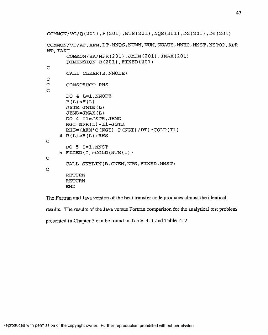
p u b l i c v o i d ASSEMB( ) { i n t 1 , i l , i ; i n t J S T R , JEND, N G I; d o u b l e RHS;d o u b l e B [ ] = n e w d o u b l e [m a x N o d e ] ; d o u b l e F I X E D [] = n e w d o u b l e [ m a x N o d e ] ;
CLEAR(B, NNO DE);
/ / C o n s t r u c t RHS
f o r (1 = 1 ; 1 <= NNODE; 1 + + ) {B[l] = F[l];JST R = J M I N [ 1 ] ;JEND = J M A X [1 ] ;
f o r ( i l = JSTR; i l <= JEND; i l + + ) {NGI = N F R [1 ] + i l - JST R ;RHS = (AFM*C[NGI] + P [ N G I ] / D T ) * C O L D [ i l ] ;B [ l ] = B [ l ] + RHS;
} / / E n d f o r i l } / / E n d f o r 1
f o r ( i = 1 ; i <= NNST; i + + )F I X E D [ i ] = C O L D [ N T S [ i ] ] ;
/ / p r i v a t e v o i d SKYLIN ( d o u b l e B [ ] , d o u b l e V AR [ ] , i n t NB[] , d o u b l e FIXED [ ] , i n t NBOUND)
SKYLIN (B , CNEW, N TS, FIX ED , NNST) ;} / / E nd ASSEM B0
Below is the same code bit from the Fortran program.
SUBROUTINE ASSEMBCOMMON/VP/P( 2 0 0 0 ) , C ( 2 0 0 0 ) , R ( 2 0 0 0 )COMMON/VA/COLD( 2 0 1 ) , CNEW( 2 0 1 )COMMON/VK/NNODE, NELEM, NTYPE, NTIM E, TIME, NFRMAX
Reproduced with permission of the copyright owner. Further reproduction prohibited without permission.
47
C O M M O N / V C / Q ( 2 0 1 ) , F ( 2 0 1 ) , N T S ( 2 0 1 ) , N Q S ( 2 0 1 ) , D X ( 2 0 1 ) , D Y ( 2 0 1 )
COMMON/VD/AF, AFM, D T , NNQS, NUMN, NUM, NGAUS, NNHC, N N ST , N STO P, KPR N T, TAXI
COMMON/SK/NFR( 2 0 1 ) , J M I N ( 2 0 1 ) , J M A X ( 20 1 )DIMENSION B ( 2 0 1 ) , F I X E D ( 2 0 1 )
CCALL CLEAR(B,NNODE)
CC CONSTRUCT RHSC
DO 4 L = l,N N O D E B ( L ) = F ( L )J S T R = J M IN (L )JEND=JMAX(L)DO 4 I1 = U S T R ,J E N D N G I = N F R ( L ) + I 1 - J S T RR H S = ( A F M * C ( N G I ) + P ( N G I ) / D T ) * C 0 L D ( I 1 )
4 B ( L ) = B ( L ) + R H S
C
C
DO 5 1 = 1 , NNST 5 F I X E D ( I ) = CO L D ( N T S ( I ) )
CALL S K Y L IN (B , CNEW ,NTS, F IX E D , N NST)
RETURNRETURNEND
The Fortran and Java version of the heat transfer code produces almost the identical
results. The results of the Java versus Fortran comparison for the analytical test problem
presented in Chapter 5 can be found in Table 4. 1 and Table 4. 2.
Reproduced with permission of the copyright owner. Further reproduction prohibited without permission.

48
Java - FORTRAN 77 Comparison
NodeFEM3Node(Java)
FEM 4Node(Java)
FEM6Node(Java)
FEM8Node(Java)
FEM3Node
(FORTRAN77)
FEM4Node
(FORTRAN77)
FEM6Node
(FORTRAN77)
FEM8Node
(FORTRAN77)
1 0.3012 0.2982 0.2945 0.2945 0.3012 0.2982 0.2945 0.29452 0.2804 0.2823 0.2787 0.2787 0.2804 0.2823 0.2788 0.27873 0.2291 0.2321 0.2292 0.2292 0.2291 0.2321 0.2292 0.22924 0.1392 0.1413 0.1396 0.1396 0.1392 0.1413 0.1397 0.13965 0.0000 0.0000 0.0000 0.0000 0.0000 0.0000 0.0000 0.00006 0.2644 0.2674 0.2640 0.2640 0.2644 0.2674 0.2640 0.26407 0.2171 0.2205 0.2176 0.2177 0.2171 0.2205 0.2177 0.21778 0.1326 0.1350 0.1332 0.1332 0.1326 0.1350 0.1333 0.13329 0.0000 0.0000 0.0000 0.0000 0.0000 0.0000 0.0000 0.000010 0.1800 0.1837 0.1811 0.1810 0.1800 0.1837 0.1811 0.181011 0.1116 0.1145 0.1127 0.1127 0.1116 0.1145 0.1127 0.112712 0.0000 0.0000 0.0000 0.0000 0.0000 0.0000 0.0000 0.000013 0.0714 0.0750 0.0729 0.0724 0.0714 0.0750 0.0729 0.072414 0.0000 0.0000 0.0000 0.0000 0.0000 0.0000 0.0000 0.000015 0.0000 0.0000 0.0000 0.0000 0.0000 0.0000 0.0000 0.0000
Table 4. 1 Java vs. Fortran Comparison for the Analytic Test Problem
Also, the runtime for the Java and Fortran programs are comparable. If one is interested in learning to program in Java, there are many good books on the subject. One such set of books is the Sun Microsystems series published by Prentice Hall.
Reproduced with permission of the copyright owner. Further reproduction prohibited without permission.

49
Java - FORTRAN 77 Comparison
NodeAbsolute
Difference 3 Node
Absolute Difference
4 Node
Absolute Difference
6 Node
Absolute Difference
8 Node1 0.0000 0.0000 0.0000 0.00002 0.0000 0.0000 0.0001 0.00003 0.0000 0.0000 0.0000 0.00004 0.0000 0.0000 0.0001 0.00005 0.0000 0.0000 0.0000 0.00006 0.0000 0.0000 0.0000 0.00007 0.0000 0.0000 0.0001 0.00008 0.0000 0.0000 0.0001 0.00009 0.0000 0.0000 0.0000 0.000010 0.0000 0.0000 0.0000 0.000011 0.0000 0.0000 0.0000 0.000012 0.0000 0.0000 0.0000 0.000013 0.0000 0.0000 0.0000 0.000014 0.0000 0.0000 0.0000 0.000015 0.0000 0.0000 0.0000 0.0000
Table 4. 2 Java vs. Fortran Difference for the Analytic Test Problem
Finite Element Program
The finite element solver was programmed using Java 1.2 and has been “compiled”
on Microsoft Windows; 98, NT, NT Server, 2000 Professional, and 2000 Server. Also, it
has been “compiled” on Linux versions 5.2 and 6.1. The program uses the Galerkin
MWR as a basis for the solver. It can solve problems using 3 node triangles, 6 node
triangles, 4 node quadrilaterals, and 8 node quadrilaterals. The maximum number of
elements is currently 1000, but this can be easily changed. The solver is currently 2000
plus lines of Java code.
Reproduced with permission of the copyright owner. Further reproduction prohibited without permission.

50
The GUI is written using Swing components and has been tested on Internet Explorer
4.0 and above. Also, it has been tested on Netscape 4.0 and above. The HTML code is
written to specify that the browsers use the Java 1.3 Plug-in. If the browser is not
currently using the 1.3 Plug-in, the browser is directed to the Sun Microsystems web site
to download and install it.
The GUI is displayed in a separate window form that o f the web browser and can be
scaled to the user’s liking. The GUI consists of three tabbed panels. The first panel is
used to displays the mesh and the boundary conditions associated with the problem. The
second panel displays the solution contour lines overlaid on the mesh. The user can
change the number of contour lines from 10 to 75 lines. The last panel gives the nodal
temperatures overlaid on the mesh. Screen shots of the program can be found in the
appendices.
Reproduced with permission of the copyright owner. Further reproduction prohibited without permission.

CHAPTERS
Numerical Results
We will use the following problem to compare the FDM and FEM to the analytical
solution. The solution of the two methods will be compared to the analytical solution.
The problem to be solved is shown in Fig. 5 .1 .
V
L
^(%.0) = 0 L
Fig. 5. 1 Domain of Analytic Test Problem
51
Reproduced with permission of the copyright owner. Further reproduction prohibited without permission.
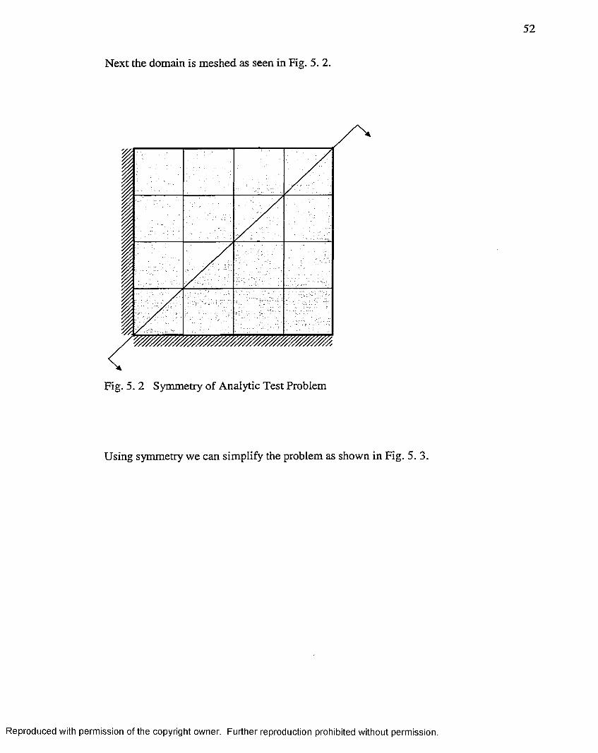
52
Next the domain is meshed as seen in Fig. 5. 2.
Fig. 5. 2 Symmetry of Analytic Test Problem
Using symmetry we can simplify the problem as shown in Fig. 5. 3.
Reproduced with permission of the copyright owner. Further reproduction prohibited without permission.

53
T = 0
Fig. 5. 3 Mesh for Analytic Test Problem
Reproduced with permission of the copyright owner. Further reproduction prohibited without permission.

54
The plot of the analytical solution using Mathematica is shown in Fig. 5. 4.
Analytical Solution
0 . 3
0 .2
tem p0 .1
Fig. 5. 4 Plot of Analytic Test Problem
The numerical data from the test problem is given in the following tables.
Reproduced with permission of the copyright owner. Further reproduction prohibited without permission.

55
Solution Comparison
Node FDMFEM 3Node(Java)
FEM 4Node(Java)
FEM 6Node(Java)
FEM 8Node(Java)
1 0.2911 0.3012 0.2982 0.2945 0.29452 0.2755 0.2804 0.2823 0.2787 0.27873 0.2266 0.2291 0.2321 0.2292 0.22924 0.1381 0.1392 0.1413 0.1396 0.13965 0.0000 0.0000 0.0000 0.0000 0.00006 0.2609 0.2644 0.2674 0.2640 0.26407 0.2151 0.2171 0.2205 0.2176 0.21778 0.1317 0.1326 0.1350 0.1332 0.13329 0.0000 0.0000 0.0000 0.0000 0.000010 0.1787 0.1800 0.1837 0.1811 0.181011 0.1110 0.1116 0.1145 0.1127 0.112712 0.0000 0.0000 0.0000 0.0000 0.000013 0.0711 0.0714 0.0750 0.0729 0.072414 0.0000 0.0000 0.0000 0.0000 0.000015 0.0000 0.0000 0.0000 0.0000 0.0000
Table 5. 1 Solution Comparison of Analytic Test Problem
Finite Element Method 3 Node (Java)
Node FiniteElement Exact Absolute
ErrorPercent
Error
1 0.3012 0.2947 0.0065 2.20562 0.2804 0.2789 0.0015 0.53783 0.2291 0.2293 0.0002 0.08724 0.1392 0.1397 0.0005 0.35795 0.0000 0.0000 0.0000 0.00006 0.2644 0.2641 0.0003 0.11367 0.2171 0.2178 0.0007 0.32148 0.1326 0.1333 0.0007 0.52519 0.0000 0.0000 0.0000 0.000010 0.1800 0.1811 0.0011 0.607411 0.1116 0.1127 0.0011 0.976012 0.0000 0.0000 0.0000 0.000013 0.0714 0.0728 0.0014 1.950014 0.0000 0.0000 0.0000 0.000015 0.0000 0.0000 0.0000 0.0000
Table 5 .2 3 Node Solution of Analytic Test Problem
Reproduced with permission of the copyright owner. Further reproduction prohibited without permission.
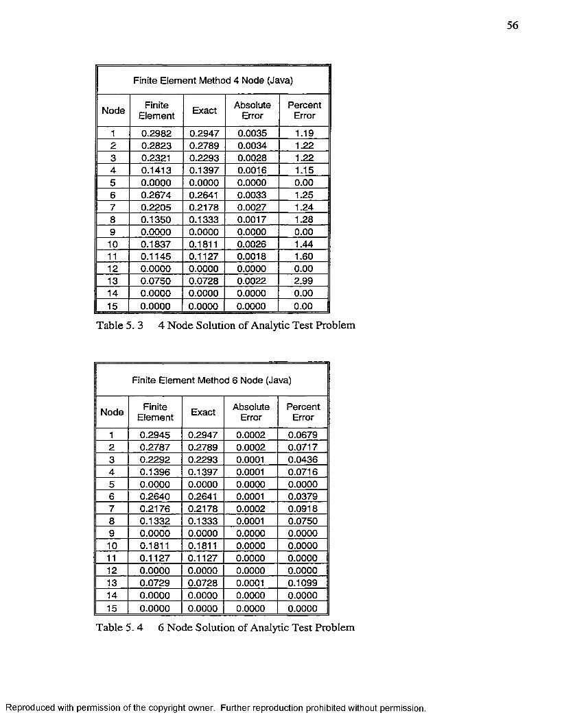
56
Finite Element Method 4 Node (Java)
Node FiniteElement Exact Absolute
ErrorPercent
Error
1 0.2982 0.2947 0.0035 1.192 0.2823 0.2789 0.0034 1.223 0.2321 0.2293 0.0028 1.224 0.1413 0.1397 0.0016 1.155 0.0000 0.0000 0.0000 0.006 0.2674 0.2641 0.0033 1.257 0.2205 0.2178 0.0027 1.248 0.1350 0.1333 0.0017 1.289 0.0000 0.0000 0.0000 0.0010 0.1837 0.1811 0.0026 1.4411 0.1145 0.1127 0.0018 1.6012 0.0000 0.0000 0.0000 0.0013 0.0750 0.0728 0.0022 2.9914 0.0000 0.0000 0.0000 0.0015 0.0000 0.0000 0.0000 0.00
Table 5. 3 4 Node Solution of Analytic Test Problem
Finite Element Method 6 Node (Java)
Node FiniteElement Exact Absolute
ErrorPercent
Error
1 0.2945 0.2947 0.0002 0.06792 0.2787 0.2789 0.0002 0.07173 0.2292 0.2293 0.0001 0.04364 0.1396 0.1397 0.0001 0.07165 0.0000 0.0000 0.0000 0.00006 0.2640 0.2641 0.0001 0.03797 0.2176 0.2178 0.0002 0.09188 0.1332 0.1333 0.0001 0.07509 0.0000 0.0000 0.0000 0.000010 0.1811 0.1811 0.0000 0.000011 0.1127 0.1127 0.0000 0.000012 0.0000 0.0000 0.0000 0.000013 0.0729 0.0728 0.0001 0.109914 0.0000 0.0000 0.0000 0.000015 0.0000 0.0000 0.0000 0.0000
Table 5. 4 6 Node Solution of Analytic Test Problem
Reproduced with permission of the copyright owner. Further reproduction prohibited without permission.

57
Finite Element Method 8 Node (Java)
Node FiniteElement Exact Absolute
ErrorPercent
Error
1 0.2945 0.2947 0.0002 0.06792 0.2787 0.2789 0.0002 0.07173 0.2292 0.2293 0.0001 0.04364 0.1396 0.1397 0.0001 0.07165 0.0000 0.0000 0.0000 0.00006 0.2640 0.2641 0.0001 0.03797 0.2177 0.2178 0.0001 0.04598 0.1332 0.1333 0.0001 0.07509 0.0000 0.0000 0.0000 0.000010 0.1810 0.1811 0.0001 0.055211 0.1127 0.1127 0.0000 0.000012 0.0000 0.0000 0.0000 0.000013 0.0724 0.0728 0.0004 0.576814 0.0000 0.0000 0.0000 0.000015 0.0000 0.0000 0.0000 0.0000
Table 5 .5 8 Node Solution of Analytic Test Problem
Finite Difference Method
Node FiniteDifference Exact Absolute
ErrorPercent
Error
1 0.2911 0.2947 0.0036 1.222 0.2755 0.2789 0.0034 1.223 0.2266 0.2293 0.0027 1.184 0.1381 0.1397 0.0016 1.155 0.0000 0.0000 0.0000 0.006 0.2609 0.2641 0.0032 1.217 0.2151 0.2178 0.0027 1.248 0.1317 0.1333 0.0016 1.209 0.0000 0.0000 0.0000 0.0010 0.1787 0.1811 0.0024 1.3311 0.1110 0.1127 0.0017 1.5112 0.0000 0.0000 0.0000 0.0013 0.0711 0.0728 0.0017 2.3414 0.0000 0.0000 0.0000 0.0015 0.0000 0.0000 0.0000 0.00
Table 5. 6 FDM Solution of Analytic Test Problem
Reproduced with permission of the copyright owner. Further reproduction prohibited without permission.

58
Percent Error Comparison
Node FDMFEM 3 Node (Java)
FEM 4 Node (Java)
FEM 6Node(Java)
FEM 8 Node (Java)
1 1.222 2.206 1.188 0.068 0.0682 1.219 0.538 1.219 0.072 0.0723 1.177 0.087 1.221 0.044 0.0444 1.145 0.358 1.145 0.072 0.0725 0.000 0.000 0.000 0.000 0.0006 1.212 0.114 1.250 0.038 0.0387 1.240 0.321 1.240 0.092 0.0468 1.200 0.525 1.275 0.075 0.0759 0.000 0.000 0.000 0.000 0.00010 1.325 0.607 1.436 0.000 0.05511 1.508 0.976 1.597 0.000 0.00012 0.000 0.000 0.000 0.000 0.00013 2.335 1.950 2.994 0.110 0.57714 0.000 0.000 0.000 0.000 0.00015 0.000 0.000 0.000 0.000 0.000
Table 5. 7 Percent Error Comparison of Analytic Test Problem
The nodal temperature distributions are shown graphically in Fig. 5. 5. The percent error
for each node can be found in Fig. 5. 6.
Reproduced with permission of the copyright owner. Further reproduction prohibited without permission.

59
Solution Values
- FDM —« — FB/13 Node FB/14 Node —x — FB/16 Node —X— FB/18 Node
0.3500
0.3000
0.2500
2 0.2000<n
o 0.1500
0.1000
0.0500
0.000010 138 9 11 12 14 154 5 6 72 31
Node
Fig. 5. 5 Solution Values of Analytic Test Problem
Reproduced with permission of the copyright owner. Further reproduction prohibited without permission.

59
Solution Values
-*— RDM —■— 3 Node F3/14 Node —x — FB/16 Node — 3K— FB/18 Node
0.3500
0.3000
0.2500
K 0.2000
o 0.1500
0.1000
0.0500
0.00005 6 7 8 92 3 4 10 11 1 2 13 141 15
Node
Fig. 5. 5 Solution Values of Analytic Test Problem
Reproduced with permission of the copyright owner. Further reproduction prohibited without permission.

60
Percent Brror
FB/Ï3 Node FB/14 Node —X— FB/16 NodeFDM
3.500
3.000
2.500
2.000
lU
1.500
1.000
0.500
0.000 412 14 15
Node
Fig. 5. 6 Percent Error of Analytic Test Problem
In the next test case we look at the analysis of a furnace wall (Incropera and DeWitt,
2001) shown in Fig. 5. 7.
Reproduced with permission of the copyright owner. Further reproduction prohibited without permission.

61
5 m
k = 0.6900W fm K
Fig. 5. 7 Brick Wall Test Problem
->1
3 m
r„= 560°C h = i m f r n ^ K
2 m 4 m
Brick
The temperature distribution in the brick wall will be found using the program created for
this thesis and a FEM program distributed by Incropera and DeWitt (2001). Using
symmetry the problem can be simplified as shown in Fig. 5. 8.
Reproduced with permission of the copyright owner. Further reproduction prohibited without permission.

62
2.5 m
1
2 m
— P\1 m
Fig. 5. 8 Symmetry of Brick Wall Test Problem
Next the domain is meshed using triangular elements as seen in Fig. 5. 9 (based on mesh configuration in Incropera and DeWitt, 2000).
13 14 15 16
12
Fig. 5. 9 Mesh of Brick WaU Test Problem
Reproduced with permission of the copyright owner. Further reproduction prohibited without permission.

63
The temperature values from the Incropera and DeWitt finite element program and the
Java based program are listed in Table 5. 8.
NodeTemp
Incropera and DeWitt
TempThesis
AbsoluteDifference
1 530.00 532.70 2.702 306.00 309.43 3.433 90.30 95.90 5.604 530.00 528.45 1.555 87.50 80.67 6.836 530.00 533.55 3.557 530.00 526.78 3.228 488.00 483.34 4.669 257.00 254.78 2.2210 308.00 308.14 0.1411 258.00 255.93 2.0712 61.10 62.78 1.6813 91.50 84.96 6.5414 88.00 87.26 0.7415 60.80 62.36 1.5616 28.10 29.03 0.93
Table 5. 8 Solution Comparison of Brick Wall Test Problem
The nodal temperature values are shown graphically in Fig. 5. 10.
Reproduced with permission of the copyright owner. Further reproduction prohibited without permission.

64
Furnace Wall
-Incropera and DeWitt —■ —Thesis
600.00
500.00
400.00
PQ.E 300.00
200.00
100.00
0.007 8 9 10 12 13 14 15 162 3 4 6 111 5
Node
Fig. 5. 10 Solution Comparison of Brick Wall Test Problem
The next test case incorporates convection, flux, and Dirichlet boundary conditions.
The domain is depicted in Fig. 5. I I .
Reproduced with permission of the copyright owner. Further reproduction prohibited without permission.

65
T =10°C
T = 120°Ck ~ 5W I mK
=50°C h = 40W fm ^K
Fig. 5. 11 Flux and Convection Test Problem
The temperature distribution will be found using the program created for this thesis. We
will then compare the distribution with the results from Hagen’s finite difference analysis
(Hagen, 1999). The mesh for the domain is shown in Fig. 5. 12
Reproduced with permission of the copyright owner. Further reproduction prohibited without permission.

66
« - . . - ' 1
17 23
,,4 !.-:J
' r -
40 J46 ^ ,I '
] 9 y . - 4 6
.;2 ; \ ,20 :
1> - i ------------, ----------- ,19k------------Ml
28
27
26
.25
24
Fig. 5. 12 Mesh for Flux and Convection Test Problem
The nodal temperature values and absolute differences are listed in Table 5 .9 .
Reproduced with permission of the copyright owner. Further reproduction prohibited without permission.

67
NodeTempHagenFDM
TempThesis
AbsoluteDifference
1 120.00 120.00 0.002 120.00 120.00 0.003 120.00 120.00 0.004 120.00 120.00 0.005 120.00 120.00 0.006 120.00 120.00 0.007 97.24 98.59 1.358 113.06 110.52 2.549 120.73 116.87 3.8610 124.85 119.48 5.3711 120.89 116.02 4.8712 104.69 99.75 4.9413 93.61 92.19 1.4214 109.63 106.62 3.0115 123.25 117.46 5.7916 135.07 125.04 10.0317 138.84 124.84 14.0018 103.70 91.84 11.8619 92.72 90.69 2.0320 109.63 106.30 3.3321 126.80 121.33 5.4722 146.20 138.39 7.8123 178.98 163.80 15.1824 92.67 90.53 2.1425 109.93 106.57 3.3626 128.44 123.15 5.2927 152.29 143.38 8.9128 182.92 173.59 9.33
Table 5. 9 Solution Comparison for Flux and Convection Test Problem
The nodal temperature values are represented graphically in Fig. 5. 13.
Reproduced with permission of the copyright owner. Further reproduction prohibited without permission.

68
I
T est Case with Flux and Convection
-e— Hagen FDM ■ -ThesB
200.00
180.00
160.00
140.00
120.00
100.00
80.00
60.00
40.00
20.00
0.001 2 3 4 5 6 7 8 9 10 11 12 13 14 15 16 17 18 19 20 21 22 23 24 25 26 27 28
Node
Fig. 5. 13 Solution Comparison for Flux and Convection Test Problem
In the next test case we will look at convection on a fin. The domain is depicted in
Fig. 5. 14.
Reproduced with permission of the copyright owner. Further reproduction prohibited without permission.

69
T„ = 25°C h= 32W lm ^K
=90°C Ki=^t6W Im K
i12 cm
7L = 25°C h = 32W I m^K
Fig. 5. 14 Fin Test Problem
The temperature distribution will be found using the program created for this thesis. We
will then compare the distribution with the one dimensional fin equation. The mesh for
the domain is shown in Fig. 5. 15.
10 11 12 13 14 15 16 17 18
Fig. 5. 15 Mesh for Fin Test Problem
The temperature values and absolute differences are listed in Table 5. 10.
Reproduced with permission of the copyright owner. Further reproduction prohibited without permission.

70
Xcoordinate
1-D Fin Equation
Temp Nodes 1 to
9
Temp Nodes 10
to 18
Abs Difference Nodes 1
to 9
Abs Difference Nodes 10
to 180.000 90.000 90.000 90.000 0 00.015 80.996 81.491 80.556 0.4954 0.93510.030 73.675 74.083 73.366 0.4081 0.71720.045 67.819 68.204 67.563 0.3857 0.6410.060 63.250 63.612 63.040 0.3624 0.5720.075 59.832 60.176 59.655 0.3448 0.52120.090 57.461 57.793 57.307 0.3321 0.48580.105 56.066 56.391 55.926 0.3246 0.4650.120 55.606 55.928 55.470 0.3221 0.4582
Table 5. 10 Solution Comparison for Fin Test Problem
The temperature values are shown graphically in Fig. 5. 16
Fin
* — 1-D Fin Equation Temp Nodes 1 to 9 —x — Temp Nodes 10 to 18
100.000
90.000
80.000
70.000
60.000
50.000
40.000
30.000
20.000
10.000
0.0000.075 0.090 0.1050.030 0.045 0.060
Length m
0.1200.000 0.015
Fig. 5. 16 Solution Comparison for Fin Test Problem
Reproduced with permission of the copyright owner. Further reproduction prohibited without permission.

CHAPTER 6
Conclusion
The finite element method is a powerful tool for solving partial differential equations
(PDE) with complicated problems domains. The method has been used to solve complex
problems in fluid flow, heat transfer, species transport, and a wide variety of structural
problems. As technology in the computer industry becomes more advanced and less
costly, we are able to solve larger and more sophisticated problems faster than ever
before. Also, with the increased computing power the meshes can be refined to yield
more accurate solutions without significantly increasing the computing time.
There are some drawbacks to using Applets. One possible solution to the problem is
Java Servlets. Using servlets one can still build cross-platform Internet solutions. Also,
with servlets there is the ability of direct access to the client and server machines. In
addition, since a servlet is running on the server side the clients hardware does not
become an issue in performance of the program. This eliminates the problem of low-end
client machines not being able to solve large problems.
The current program should provide a basis for improvement. Future plans are to add
mesh adaptation to the program. Adaptation allows the mesh to be refined in places
where there may be a steep gradient. Also, interaction with the mesh and the user will be
71
Reproduced with permission of the copyright owner. Further reproduction prohibited without permission.

72
added. This interaction will allow the user to move nodes and specify boundary
conditions on the fly. Lastly, radiation and 3-D capability will be added to the program.
Reproduced with permission of the copyright owner. Further reproduction prohibited without permission.

APPENDICES
Notation
du
d^u u„ =-dx^
" ■ i * f
dT dT dT a n ~ 3 x " " '^ a y ”"
Here n, and n„ are the direction cosines of the unit outward vector, normal to a giveny
boundary.
73
Reproduced with permission of the copyright owner. Further reproduction prohibited without permission.

74
Analytic Solution
Substituting (2. 8) into the governing equation (2. 3) we get
K [a {x)+ u„ + b"{y) + UyJ\ + Q = Q
A homogeneous equation for u [x ,y ) can be obtained by taking
( 1)
Equation (1 ) implies that
K \_a{x)+ b ''{y) + Q = 0]
where a '(x ) = - ^ ^ a [ x ) . Assuming Q is a constant we can satisfy the above equation by
letting
K a { x ) + Q = 0 (2)
and
^ '(y ) = 0 (3)
Substituting (2. 8) into the boundary condition (2. 4) gives
a '(0 ) + M_^(0,y) = 0
where a(^x) = ( x ) . To obtain a homogeneous boundary condition for u (x, y) let
«x(0>3') = 0 (4)
The above dictates that we take
a '(0 )= 0 (5)
Substituting (2. 8) into (2. 5) gives
Reproduced with permission of the copyright owner. Further reproduction prohibited without permission.

75
a (L )+ & (y )+ « (L ,y )= r^
To obtain a homogeneous boundary condition for u (x, y ) let
M(L,y) = 0 (6)
This implies that we must also satisfy
a{L)-hb{y)= T^
From the above equation we see 6 (y ) is a constant satisfying ( 3). Now we take
a{L )= T , (7 )
and
b {y )= 0 (8)
Substituting (2. 8) into (2. 6) yields
b'(p) + Uy (x,0) =0
Because we took b [y )= 0 in ( 8), we see that 6 '(0) = 0 and
M y(x,0)=0 (9)
Substimting (2. 8) into the last boundary condition we have
a (x )+ 6 (L ) + w(x,L) = T^
Solving for u (x, L) and letting b[L) = 0 from ( 8) we have
M (x, L) = — a (x) ( 10)
We now summarize the sub problems and the boundary conditions that must be solved
Reproduced with permission of the copyright owner. Further reproduction prohibited without permission.

Æ a'(x) + G = 0
a{Q) = 0
a ( L ) = r ,
6 '(y ) = 0
6(y) = 0
“ « + “ y y = 0
“x(0>3')=0
M(Z,,y) = 0
M y(x,0)=0
76
(2)
(5)
(7)
(3)
( 8)
( 1)
(4)
( 6)
(9)
m(x,L) = r^-<z(x) (10)
Equation ( 2) is an ordinary differential equation and can be solved by integration
twice, applying the boundary conditions ( 5) and ( 7). This yields the following result
= ( U )
Substituting the result into ( 10) we have
( 12)Q
2K
Equation ( 8) is the solution for 6 (y ) and satisfies ( 3). Substituting (11) and ( 8) into
(2. 8) we get
Reproduced with permission of the copyright owner. Further reproduction prohibited without permission.

77
T { x ,y ) = T ^ + ^ { Û - x ^ ) + u { x .y ) (13)
For readability we will summarize the sub problems in T [x ,y ) and u (x, y) that are
left to solve.
T { x , y ) = T ^ + ^ [ L ^ - x ^ ) + u { x , y )(13)
« . + ^ . = 0 ( 1)
“x(0’3 ')= 0 (4)
( 6)
“y (-^>0) = 0 (9)
■‘ { x .L ) = - ^ { x ^ - Û ) (12)
The method of separation of variables can now be used to find m (x, y ) . To use the
method assume the solution has the form of
u {x ,y ) = Y { y )X { x ) (14)
Substituting the assumed solution into ( 1) yields
% '(x)y (y ) + Z ( x ) r ( y ) = 0
After rearranging the equation we have
£ I W = - I 1 WX (x ) Y {y)
The only way for the equality to hold is if both sides are equal to a constant. Taking the
constant to be —À~ we let
Reproduced with permission of the copyright owner. Further reproduction prohibited without permission.
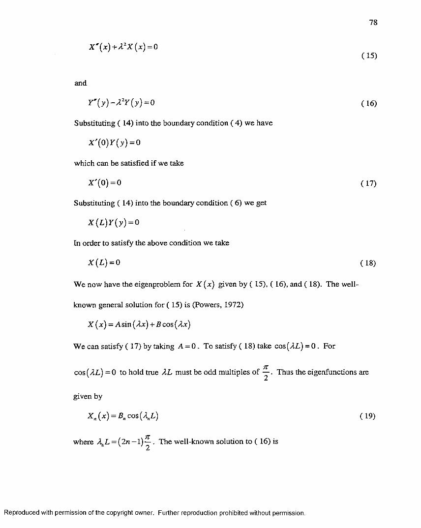
X \ x ) + À - X { x ) = Q
78
(15)
and
r ( y ) - / l " y ( y ) = 0 (16)
Substituting ( 14) into the boundary condition ( 4) we have
z ' ( o ) r ( y ) = o
which can be satisfied if we take
X '(0 ) = 0 (17)
Substituting ( 14) into the boundary condition ( 6) we get
X ( L ) r ( y ) = 0
In order to satisfy the above condition we take
X ( L ) = 0 (18)
We now have the eigenproblem for X (x) given by ( 15), ( 16), and ( 18). The well-
known general solution for ( 15) is (Powers, 1972)
X (x) = A sin (/Ix) -h B cos (Àx)
We can satisfy ( 17) by taking A = 0 . To satisfy ( 18) take cos (ÀL) = 0 . For
7tcos (AT) = 0 to hold true XL must be odd multiples of —. Thus the eigenfunctions are
given by
X ,(x ) = B,cos(A.i.) (19)
where = (2 n —l ) - ^ . The well-known solution to ( 16) is
Reproduced with permission of the copyright owner. Further reproduction prohibited without permission.

79
^ ( y ) = Q sinh(A„y) + D„ cosh(A„y) ( 20)
Substituting ( 19) and ( 20) into ( 14) we obtain
«n y) = cos(A„x) [C„ sinh (A„y) + 0„ cosh(A„y)]
where is now part of C„ and Z)„. By summing over all the eigenvalues a more
general solution can be given by
= f ]c o s (A„x) [C„ sinh (A„y) + D„ cosh (A„y )] ( 21)r t= l
The expression for C„ and will be taken to make (21) satisfy the boundary
conditions ( 9) and ( 12). After differentiating ( 21) with respect to y, we have
Uy(x,y) = '^cos(A „x)[C„„ cosh(A„y) + D„A„ sinh(A„x)]n—0
Then by setting y = 0 and substituting into ( 9) we have
Zcos(A„x)C„A„ =0n=l
The only way for this equation to be satisfied for all x is to take C„ = 0 . Thus (21)
reduces to
J') = Z ^ o s (A,x) cosh (A,y ) (22)n = l
Letting y = L and substituting ( 22) into ( 12) we get
Jcos(A „x)D „ cosh(A„y) )n = l
Multiplying both sides by cos (A^x) dx and integrating form x = 0 to x — L we obtain
D„. Thus we have
Reproduced with permission of the copyright owner. Further reproduction prohibited without permission.
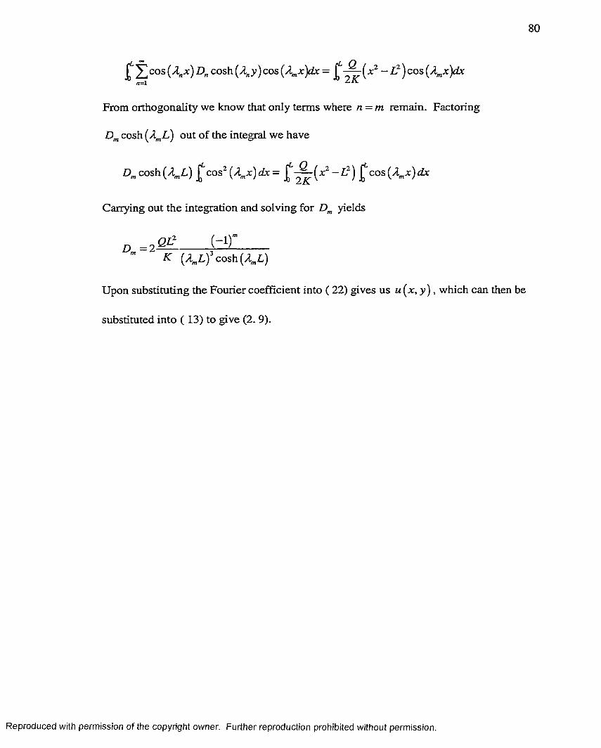
80
Ê cos(A„x) D„ cosh(A„y)cos(A„x)dx = ^ ^ ( x ^ - L ^ ) c o s ( A „ x ) d x/ i= l
From orthogonality we know that only terms where n = m remain. Factoring
cosh (A„L) out of the integral we have
cosh (A„L) cos^ (A„x) dx = - L^) cos (A^x) dx
Carrying out the integration and solving for yields
D „ = 2 ^ t l T ----------X (A„L) cosh (A^L)
Upon substituting the Fourier coefficient into ( 22) gives us u (x, y ) , which can then be
substituted into ( 13) to give (2. 9).
Reproduced with permission of the copyright owner. Further reproduction prohibited without permission.

Units
81
Quantity Symbol SI English
Area A ivAConvective transfer coefficient h W lrn^ °C B tu /h r ft^ °F
Density P kg I 16m/.A'Heat energy q kJ BtuForce F N lb,
Gravity 8 m l f t !Heat flux per unit area q ! A W lm - Btu / hr JiAHeat generation per unit length Q Wlrn^ Btu ! hr ft^
Length L m f t
Mass m kg IKPressure P N/rn^ lb, ! irC'
Specific heat k J Ik g °C Btullb^ °FThermal conductivity K W /m °C Btu /h r f t °F
Thermal diffusivity cc{k I pc^) I s f t ^ / s
Velocity V m ! s f t ! s
Reproduced with permission of the copyright owner. Further reproduction prohibited without permission.

82
Program Screen Shot of Tab One
Domain Mesh
2-D FEM H ea t T ra n sfe r by T revor Wilcox a n d D arrell P e p p e r
«a
^ 0* G M * m 0 K S a a R K H R ^ ^vS :iJ.-i.'‘
*!£,4S3sS!t.SS
am
Reproduced with permission of the copyright owner. Further reproduction prohibited without permission.

Program Screen Shot of Tab Two
83
Solution Contours
2-D FEM H ea t T ransfer by T revor Wilcox a n d D arrell P ep p er
Reproduced with permission of the copyright owner. Further reproduction prohibited without permission.

Program Screen Shot of Tab Three
Solution Values
84
.qk
#Qg3@ M S #39iQ44>4i"38% Pâ%S%53
Reproduced with permission of the copyright owner. Further reproduction prohibited without permission.

Gauss Points for Triangular Elements
85
3 Node Triangular ElementGauss Point A A A W
1 0-5 0 0.5 0.333333332 0.5 0.5 0 0.333333333 0 0.5 0.5 0.33333333
6 Node Triangular ElementGauss Point A A A W
1 0.33333333 0.33333333 0.33333333 0.2252 0.47014206 0.05971587 0.47014206
0.132394153 0.47014206 0.47014206 0.059715874 0.05971587 0.47014206 0.470142065 0.10128651 0.79742699 0.10128651
0.125939186 0.10128651 0.10128651 0.797426997 0.79742699 0.10128651 0.10128651
Reproduced with permission of the copyright owner. Further reproduction prohibited without permission.

Gauss Points for Quadrilateral Elements
86
4 Node Quadrilateral ElementsGauss Points Vi
1 11 .
V3 VF1 1
1 12
S VF1 1
1 11 13
VF VF1 1
1 14VF
8 Node Quadrilateral ElementsGauss Points
-I -I 59
0
-I I _59
0 -I 59
0 059
59
09
59
59
59
0 59
59
I 59
59
Reproduced with permission of the copyright owner. Further reproduction prohibited without permission.

87
GUI Flow Chart
CreatePanel
Is FEM True
Is Mesh True
YesYes
PaintContour
Lines
Do FEMLoad File
PaintTempValues
SolveFEM
ContourLines
Number
Set Mesh True
RepaintContour
Lines
Set FEM True
Reproduced with permission of the copyright owner. Further reproduction prohibited without permission.

88
Solver Flow Chart
Data FilesINIT
No
IAX1 = 0
Yes
SHAPE
BNDAXI
SHAPE
NODSET
BCSIDE
MATAXI
Set arrays to zero. Read data.
CLEAR
GAUSS
BCSIDE
KOUNT = 0 NTIME = 0 TIME = DT
NODSET
SHAPE
Reproduced with permission of the copyright owner. Further reproduction prohibited without permission.

89
for NSTEP = 1 to NSTOP
KOUNT= KPRNT
Yes
No
SHAPE
SHAPE
BCSIDE
NODSET
CLEAR
SKYLIN
SHAPE
BCSIDE
PRINT KOUNT= 0
NODSET
ASSEMB
BNDCON
MATSET
TIME = TIME+ DT KOUNT = KOUNT+1 NTIME = NTIME + 1
Reproduced with permission of the copyright owner. Further reproduction prohibited without permission.

90
RESID
L = 1 to NNODE
Output
End
Reproduced with permission of the copyright owner. Further reproduction prohibited without permission.

91
Sample Input Data File
D a t a s e t T i t l e : L IN -2 D 4 .D A T1 MTYPE2 NUMDIM N u m b er o f d i m e n s i o n s 2 5 NNODE N u m b er o f n o d e s1 6 NELEM N u m b er o f e l e m e n t s4 NUMN N u m b er o f N o d e s p e r E l e m e n t 1 0 0 NSTOP M ax N o . o f i t e r a t i o n s5 0 KPRNT P r i n t i n g i n t e r v a l1 NVEL ( 0 ) n o v e l o c i t i e s o r ( 1 ) v e l o c i t y d a t a s e t e x i s t s2 NTYPE ( 1 ) S t e a d y - s t a t e o r ( 2 ) t i m e - d e p e n d e n t 0 . 1 0 DT T im e s t e p1 . 0 A F ( 1 . 0 ) I m p l i c i t o r ( 0 . 5 ) C r a n k - N i c o l s o n 0 . 0 TO1 . 0 1 . 0 0 1 . 0 1 . 0
RHOCPlA X I (0 ) C a r t e s i a n o r (1 ) A x i s y m m e t r i cm ax X m ax y. c o o r d i n a t e s
1 0 . 0 0 0 0 0 0 . 0 0 0 0 02 0 . 0 0 0 0 0 0 . 2 5 0 0 03 0 . 0 0 0 0 0 0 . 5 0 0 0 04 0 . 0 0 0 0 0 0 . 7 5 0 0 05 0 . 0 0 0 0 0 1 . 0 0 0 0 06 0 . 2 5 0 0 0 0 . 0 0 0 0 07 0 . 2 5 0 0 0 0 . 2 5 0 0 08 0 . 2 5 0 0 0 0 . 5 0 0 0 09 0 . 2 5 0 0 0 0 . 7 5 0 0 0
1 0 0 . 2 5 0 0 0 1 . 0 0 0 0 01 1 0 . 5 0 0 0 0 0 . 0 0 0 0 01 2 0 . 5 0 0 0 0 0 . 2 5 0 0 01 3 0 . 5 0 0 0 0 0 . 5 0 0 0 01 4 0 . 5 0 0 0 0 0 . 7 5 0 0 01 5 0 . 5 0 0 0 0 1 . 0 0 0 0 01 6 0 . 7 5 0 0 0 0 . 0 0 0 0 01 7 0 . 7 5 0 0 0 0 . 2 5 0 0 01 8 0 . 7 5 0 0 0 0 . 5 0 0 0 01 9 0 . 7 5 0 0 0 0 . 7 5 0 0 02 0 0 . 7 5 0 0 0 1 . 0 0 0 0 02 1 1 . 0 0 0 0 0 0 . 0 0 0 0 02 2 1 . 0 0 0 0 0 0 . 2 5 0 0 02 3 1 . 0 0 0 0 0 0 . 5 0 0 0 02 4 1 . 0 0 0 0 0 0 . 7 5 0 0 02 5 1 . 0 0 0 0 0 1 . 0 0 0 0 0
Reproduced with permission of the copyright owner. Further reproduction prohibited without permission.

92
1 . 0 0 1 5 . 00 1 5 . 0 0 1 6 7 22 . 0 0 1 5 . 00 1 5 . 0 0 2 7 8 33 . 0 0 1 5 . 0 0 1 5 . 0 0 3 8 9 44 . 00 1 5 . 0 0 1 5 . 0 0 4 9 10 55 . 0 0 1 5 . 0 0 1 5 . 00 6 1 1 12 76 . 0 0 1 5 . 0 0 1 5 . 0 0 7 12 13 87 . 0 0 1 5 . 00 1 5 . 00 8 13 1 4 98 . 0 0 1 5 . 0 0 1 5 . 00 9 1 4 15 1 09 . 00 1 5 . 0 0 1 5 . 0 0 1 1 1 6 17 12
1 0 . 00 1 5 . 0 0 1 5 . 0 0 12 17 18 131 1 . 0 0 1 5 . 0 0 1 5 . 0 0 13 18 19 1 41 2 . 00 1 5 . 0 0 1 5 . 00 1 4 19 2 0 1 513 . 00 1 5 . 0 0 15 . 0 0 1 6 2 1 2 2 1 71 4 . 0 0 1 5 . 0 0 1 5 . 0 0 1 7 2 2 23 1 81 5 . 0 0 1 5 . 0 0 1 5 . 0 0 18 23 2 4 1 91 6 . 00 1 5 . 0 0 1 5 . 0 0 19 2 4 25 2 0
DIRCFLUX
1 1 0 0 0 . 0 02 1 0 0 0 . 0 03 1 0 0 0 . 0 04 1 0 0 0 . 0 05 1 0 0 0 . 0 0
1 2 0 . 0 0 1 5 0 0 . 0 0 1 41 2 0 . 0 0 1 5 0 0 . 0 0 4 21 2 0 . 0 0 1 5 0 0 . 0 0 5 41 2 0 . 0 0 1 5 0 0 . 0 0 8 21 2 0 . 0 0 1 5 0 0 . 0 0 9 41 2 0 . 0 0 1 5 0 0 . 0 0 12 21 2 0 . 0 0 1 5 0 0 . 0 0 13 31 2 0 . 0 0 1 5 0 0 . 0 0 13 41 2 0 . 0 0 1 5 0 0 . 0 0 1 6 21 2 0 . 0 0 1 5 0 0 . 0 0 1 6 3
CONVVELC
Reproduced with permission of the copyright owner. Further reproduction prohibited without permission.

BIBLIOGRAPHY
Brebbia, C. and Dominguez, J., 1989, Boundary Elements an Introductory Course, Computational Mechanics Publication, Boston.
Comini, G., Giudice, S. D., and Nonino, C, 1994, Finite Element Analysis in Heat Transfer, Taylor & Francis, Washington.
Fletcher, C.A.J, 1991, Computational Techniques fo r Fluid Dynamics, Volume II, Springer-Verlag, New York.
Geary, D., 1999, Graphic Java Mastering the JFC, AWT, Third Ed., Prentice Hall, California.
Geary, D., 1999, Graphic Java Mastering the JFC, Swing, Third Ed., Prentice Hall, CaUfomia.
Gerald, C., 1978, Applied Numerical Analysis Second Ed., Addison Wesley, Philippines.
Hagen, K., 1999, Heat Transfer with Applications, Prentice Hall, New Jersey.
Horstmann, C., 1999, Core Java Vol. I, Fundamentals, Prentice Hall, California.
Incropera, F. and DeWitt, D., 1996, Fundamentals o f Heat and Mass Transfer, Fourth Edition, John Wiley & Sons, New York.
Incropera, F. and DeWitt, D., 2000, Problem Set Supplement and Software Tools, John Wiley & Sons, New York.
93
Reproduced with permission of the copyright owner. Further reproduction prohibited without permission.

94
Myers, G., 1998, Analytical Methods in Conduction Heat Transfer Second Ed., AMCHT, Wisconsin.
Ozi§ik, N., 1993, Heat Conduction, Second Ed., John Wiley & Sons, Inc., New York.
Pepper, D. and Heinrich, J., 1992, The Finite Element Method, Basic Concepts and Applications, Taylor & Francis, Washington.
Powers, D., 1972, Boundary Value Problems, Third Ed., Harcourt Brace College Publishers, Fort Worth.
Thompson, J., Warsi, Z., and Mas tin, C., 1985, Numerical Grid Generation, North- Holland, New York.
Reproduced with permission of the copyright owner. Further reproduction prohibited without permission.

VTTA
Graduate College University of Nevada, Las Vegas
Trevor A. Wilcox
Local Address:110 Quiet Desert Ln Henderson, NV 89014
Home Address:6635 Lunar Drive Anchorage, AK 99504
Degrees:Bachelor of Science, Mathematics, 1997 University of Alaska, Anchorage
Master of Science, Mathematics, 1998 University of Nevada, Las Vegas
Thesis Title: A Web Based Finite Element Model for Heat Transfer
Thesis Examination Committee:Chairperson, Dr. Darrell Pepper Committee Member, Dr. Mohamed Trabia Committee Member, Dr. Yi-Tung Chen Graduate Faculty Representative, Dr. Laxmi Gewali
95
Reproduced with permission of the copyright owner. Further reproduction prohibited without permission.