Embed Size (px)
Citation preview

- 1 -
Finite Element Analysis of the Heat Transfer in a Copper Mould during Continuous Casting of Steel Slabs
14 May 2005
D. Hodgson, Sami Vapalahti, and B.G. Thomas
Department of Mechanical and Industrial Engineering University of Illinois at Urbana-Champaign
Urbana, IL 61801 [email protected]

- 2 -
Abstract
To calibrate the CON1D model for accurate simulation of mold temperature and heat
flux in a thin-slab casting mold, 3-dimensional heat transfer computations were
performed using ANSYS and used to find the offset distance for CON1D. The
CON1D model was found to produce accurate simulations everywhere across the
wideface, so long as the mold thickness is set to 33.4mm and the thermocouple
positions are offset by 1.8mm (moving thermocouples computationally from 14mm to
12.2mm from the hot face). Thermocouple temperatures drop greatly if there is any
contact problem attaching them (~10 oC drop for just a contact resistance equivalent
to 0.01mm air gap)
Introduction
Copper continuous casting moulds are used heavily in steel production to
produce high quality steel sheets from molten steel. These sheets are produced by
pouring the molten steel into the mould which removes enough heat to solidify the
outer layers into a solid steel shell. The partially solid steel is removed at a constant
rate, allowing the steel to be continuously poured into the mould, finishing
solidification further along the casting system. Due to the high temperatures involved
in the process, the copper is cooled by pumping cooling water through slots within the
mould. This is monitored by thermocouples placed at regular intervals throughout the
mould.
The thermocouples are there to note any unexpected temperature rises, which
could be indications of unusual cooling flow, leading to damage to the copper. This is
important as any damage to the copper could create cracks, which if they were
allowed to propagate to the cooling slots, cause catastrophic failure. The necessary
safety and working life considerations mean that the thermocouples are set back from
the hot face of the mould. It is therefore necessary to have an understanding of the
temperature distribution and heat flux within the mould to know the relationship
between the hot face temperature and the measured temperature at the thermocouples.

- 3 -
This is initially an investigation into the temperature distribution with a small, 5mm
thick section.
This was followed by investigating the effect of the thermocouple placement
holes on the temperature distribution as well as the cooling effect of the thermocouple
wire by conducting heat away from the mould. This cooling effect could lead to
inaccurate readings from the thermocouple and a slightly different temperature
distribution through the mould. As before the model will be a 5mm section of the
mould.
This data developed from these simulations can be used to find what is known
as offset values for this mould. These offset values are used to allow a simple
simulation, in this case CON1D1 which is a FORTRAN simulation, to be used to
predict this more complex mould. These offset values will be reasonably constant and
would be specific to this mould. To help find these offset values the simulation will
be run at different depths the temperature profile investigated. The depths looked at
will be 800mm, 400mm and 110mm below the meniscus
To allow easier referencing the initial investigation will be referred to as Case
1 at 800mm below the meniscus. The following investigation into the effect of the
thermocouple hole and the cooling effect of the thermocouple wire will be referred to
as Case 2 and 3 respectively, both at 800mm. The simulations at different depths will
be Case 2 for 400mm and 110mm. A fourth case will also be looked at investigating
the effect of the mould thickness.
The final investigation of this study will be to create a 3-D simulation of the
mould expanding the domain to a 130mm section rather than the thin section used
previously. This will allow the inclusion of a varying heat flux in relation to the
depth. As the steel cools the amount of heat being absorbed by the mould reduces. In
the case of the casting mould this means that the heat flux is at a maximum at the
meniscus and reduces as the depth below the meniscus increases. This larger model
will investigate the interaction of this varying heat flux on the temperature profile
within the mould.
Model Description
The equation being solved is the 3-D heat conduction equation shown below:
- 4 -
0=∂∂
∂∂
+∂∂
∂∂
+∂∂
∂∂
zTk
zyTk
yxTk
x
This will be solved using ANSYS 8.02 for the first simple domains of an
Algoma mould and the domain is described below. The final simulation of a 3-D
section will be modelled using FEMLAB3 as this program’s license allows a larger
number of nodes and elements.
Domain
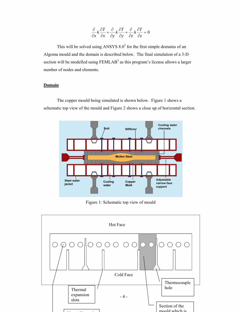
The copper mould being simulated is shown below. Figure 1 shows a
schematic top view of the mould and Figure 2 shows a close up of horizontal section.
Figure 1: Schematic top view of mould
Thermocouple hole Thermal
expansion slots
Hot Face
Cold Face
W Ch l
Section of the mould which is
- 5 -
Figure 2: Close up of horizontal section
In Figure 2 the circular pipes are the cooling water tubes rather than the
rectangular slots common in mould design. The rectangular slots are structural
expansion slots and therefore have negligible heat transfer effects. These expansion
slots are designed to allow the thermal expansion of the hot face during operation to
lessen constraint caused by the cold side thereby lowering operational stresses and
residual stress. It can be seen that there is slightly greater spacing between the bored
holes that straddle the thermocouple holes to allow them to fit.
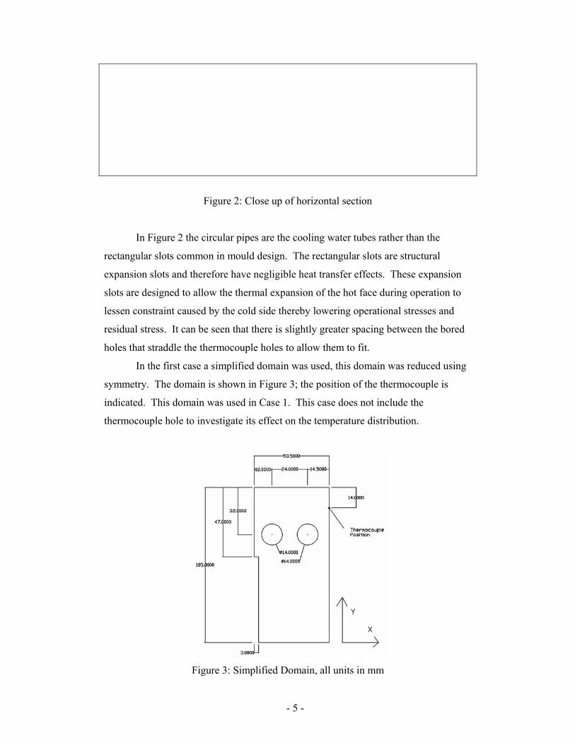
In the first case a simplified domain was used, this domain was reduced using
symmetry. The domain is shown in Figure 3; the position of the thermocouple is
indicated. This domain was used in Case 1. This case does not include the
thermocouple hole to investigate its effect on the temperature distribution.
Figure 3: Simplified Domain, all units in mm
- 6 -
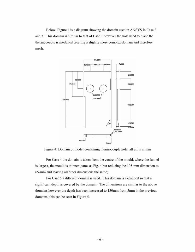
Below, Figure 4 is a diagram showing the domain used in ANSYS in Case 2
and 3. This domain is similar to that of Case 1 however the hole used to place the
thermocouple is modelled creating a slightly more complex domain and therefore
mesh.
Figure 4: Domain of model containing thermocouple hole, all units in mm
For Case 4 the domain is taken from the centre of the mould, where the funnel
is largest, the mould is thinner (same as Fig. 4 but reducing the 105-mm dimension to
65-mm and leaving all other dimensions the same).
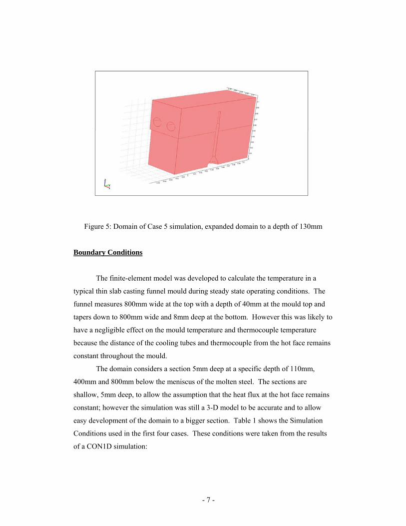
For Case 5 a different domain is used. This domain is expanded so that a
significant depth is covered by the domain. The dimensions are similar to the above
domains however the depth has been increased to 130mm from 5mm in the previous
domains; this can be seen in Figure 5.
- 7 -
Figure 5: Domain of Case 5 simulation, expanded domain to a depth of 130mm
Boundary Conditions
The finite-element model was developed to calculate the temperature in a
typical thin slab casting funnel mould during steady state operating conditions. The
funnel measures 800mm wide at the top with a depth of 40mm at the mould top and
tapers down to 800mm wide and 8mm deep at the bottom. However this was likely to
have a negligible effect on the mould temperature and thermocouple temperature
because the distance of the cooling tubes and thermocouple from the hot face remains
constant throughout the mould.
The domain considers a section 5mm deep at a specific depth of 110mm,
400mm and 800mm below the meniscus of the molten steel. The sections are
shallow, 5mm deep, to allow the assumption that the heat flux at the hot face remains
constant; however the simulation was still a 3-D model to be accurate and to allow
easy development of the domain to a bigger section. Table 1 shows the Simulation
Conditions used in the first four cases. These conditions were taken from the results
of a CON1D simulation:
- 8 -
Table 1: Simulation Conditions
Boundary Condition in all Cases Thermal conductivity of copper 372 W m-1K-1 Distance of thermocouple from hot face 14mm Remaining faces of model Perfectly insulated Water Velocity in bored holes 8.7 m/s Boundary Conditions at Individual Depths Depth below meniscus (mm) 110 400 800 Heat Flux (MW m-2) 3.18 2.201 1.704 Water tube heat transfer coefficient (kW m-2K-2) 32.4412 34.6691 35.7748 Water temperature (°C) 21.31 25.00 28.31
Note that the heat transfer coefficient varies with position in the mould. The
coefficient increases as the depth increases due to heating of the water.
The results of these simulations will be divided into five different cases:
Case 1) No thermocouple hole present in domain.
Case 2) The thermocouple hole included in domain though the
cooling effect of the thermocouple wire was not
included.
Case 3) Both the thermocouple hole and the cooling effect are
modelled in the domain.
Case 4) Case 2 with 65-mm thick mould section, (vs. 105 mm
mould section) smaller domain.
Case 5) Similar dimensions to previous cases however domain
has been expanded to a depth of 130mm.
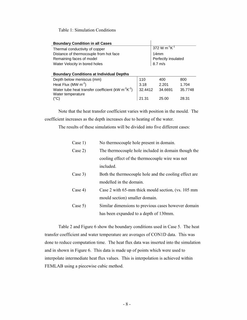
Table 2 and Figure 6 show the boundary conditions used in Case 5. The heat
transfer coefficient and water temperature are averages of CON1D data. This was
done to reduce computation time. The heat flux data was inserted into the simulation
and in shown in Figure 6. This data is made up of points which were used to
interpolate intermediate heat flux values. This is interpolation is achieved within
FEMLAB using a piecewise cubic method.
- 9 -
Table 2: The boundary conditions used in Case 5
Boundary conditions for Case 5 Water tube heat transfer coefficient (kW m-2K-2) 34712.16Water temperature(°C) 25.50347
Plot of input heat flux with respect to depth
0.000E+00
1.000E+06
2.000E+06
3.000E+06
4.000E+06
5.000E+06
-0.2 0 0.2 0.4 0.6 0.8 1
Depth (m)
Hea
t flu
x (M
W/m
^2)
Figure 6: Plot showing the change of heat flux as depth increases. This is the data
used for Case 5
The first three cases were investigated at 800mm to allow comparison and
investigate the effect of the thermocouple on the temperature distribution. From these
results it was decided to compare Case 2 at various depths, 110mm and 400mm to
investigate how the results differ from those calculated using CON1D. These results
can be used to calculate off-set values to allow the faster running CON1D simulation
to predict temperatures for the mould.
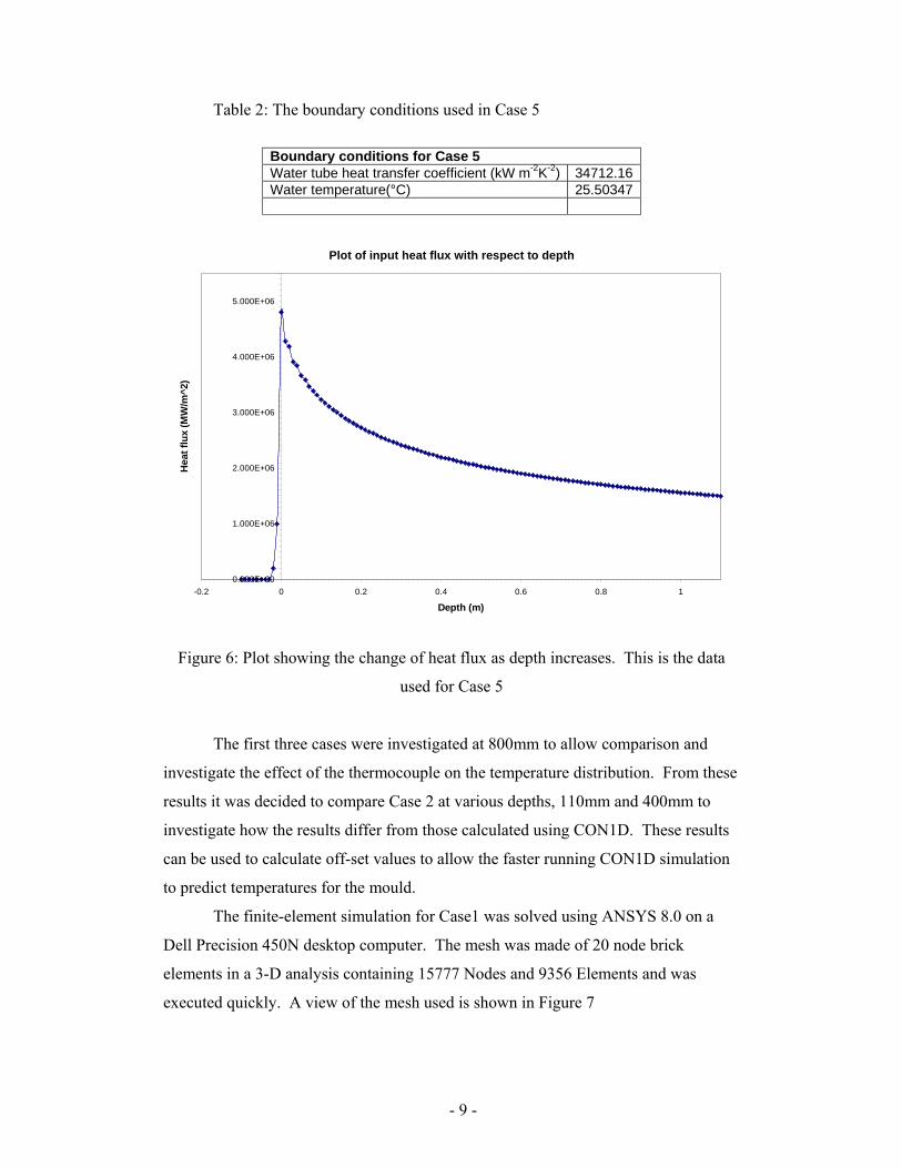
The finite-element simulation for Case1 was solved using ANSYS 8.0 on a
Dell Precision 450N desktop computer. The mesh was made of 20 node brick
elements in a 3-D analysis containing 15777 Nodes and 9356 Elements and was
executed quickly. A view of the mesh used is shown in Figure 7
- 10 -
Figure 7: Mesh of Case 1, containing 9931 nodes and 17434 elements
Notice that the mesh has been refined in the vicinity of the thermocouple; this
creates ~20 elements from the hot face to the thermocouple.
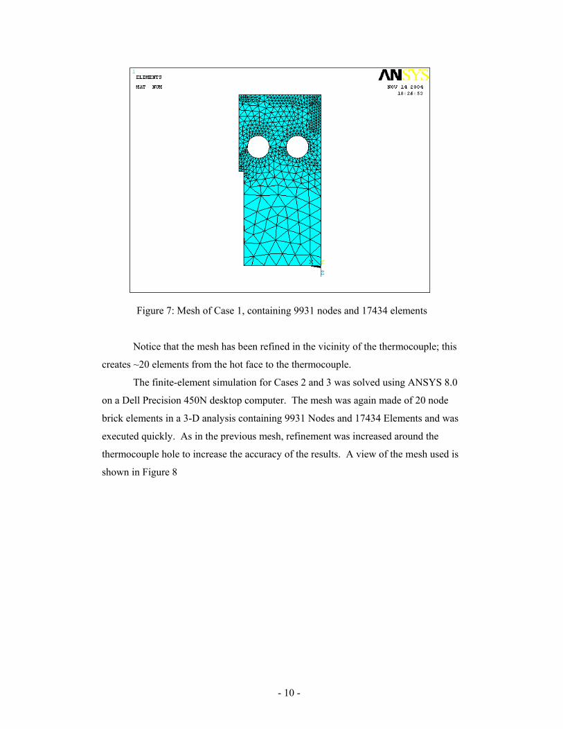
The finite-element simulation for Cases 2 and 3 was solved using ANSYS 8.0
on a Dell Precision 450N desktop computer. The mesh was again made of 20 node
brick elements in a 3-D analysis containing 9931 Nodes and 17434 Elements and was
executed quickly. As in the previous mesh, refinement was increased around the
thermocouple hole to increase the accuracy of the results. A view of the mesh used is
shown in Figure 8
- 11 -
Figure 8: View of mesh used for Cases 2 and 3, containing 3140 Nodes and 12926
Elements
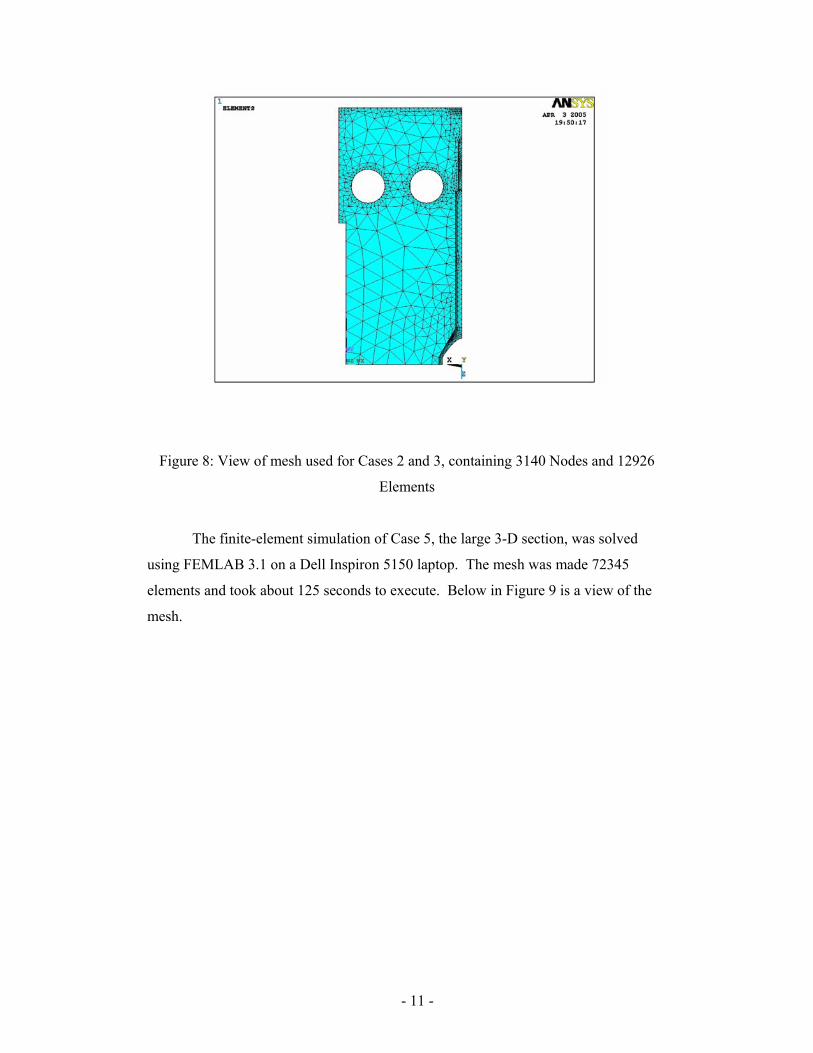
The finite-element simulation of Case 5, the large 3-D section, was solved
using FEMLAB 3.1 on a Dell Inspiron 5150 laptop. The mesh was made 72345
elements and took about 125 seconds to execute. Below in Figure 9 is a view of the
mesh.

- 12 -
Figure 9: View of the mesh for Case 5, large 3-D section
Calculating the Cooling Effect of the Thermocouple Wire
The cooling effect was investigated in Case 3 using an iterative method based
on a wire divided into two sections with different conditions along each section. In
Figure 10 a diagram of the wire model is shown.
Figure 10: Diagram of the wire model used to calculate the cooling effect
The first section was treated as a conductive wire with a fixed temperature at
one end. It was assumed that no heat loss occurred from the surface as the ambient
Convection into water jacket. h, T∞
∆Y∆y
T1 T2
No heat loss through this section
q

- 13 -
temperature would be similar to the wire due to the air being heated by the
surrounding mould. This is connected to the second section where heat loss occurs by
convection. All the heat transported down the wire is assumed to be lost through this
section. The iteration is necessary as the initial temperature difference in the first
section is estimated. Repeated calculations are made to refine this temperature
difference. No conduction along the wire in the convective section was calculated to
simplify the process. Below is an example calculation with the conditions shown in
Table 3.
Table 3: Conditions used in iterative calculation
T1 139°C T2 34°C T∞ 28.31°C h 20000 Wm-2K-1 k 22 Wm-1K-1 ∆y 0.103m ∆Y 0.2m Diameter, D 0.003m Area, A 7.0686 × 10⁻⁶ m2 Perimeter area in convective section, P 0.001884 m2
( )( ) ( )
C28.3142
found becan thisfrom001884.0)31.28(200001585290
)(hqdifference etemperaturnecessary find section to second through lossHeat :nCalculatio
1585290103.0
100686.710522sectionfirst along Conduction :nCalculatio
)()(k
q
match tofluxesheat forcing respect to with following thesolve toisn calculatio iterative thisof purpose The
2
2
2
2
621
221con
2
°=
×−×=
×−×=
=
×××=
×−×=
−=∆
−=
∞
−
∞
new
new
new
new
T
TT.
PTT
W.qdy
ATTkq
TThPy
TTA
T
From this new T2 value a new (T1-T2) is found, 110.686°C. This means a new

- 14 -
q needs to be calculated and the process is repeated. Eventually this settles on a value
for T2of 28.31443°C and the amount of heat transported down the wire is 0.167112W.
The simplification of the calculation by not modelling the conduction along
the wire in the water cooled section has the added benefit of causing the value to be
an upper bound. In reality the heat loss down the wire is less than calculated as the
temperature at the end of the first section would be higher leading to less heat
conducted down the wire.
This method assumes that the wire end has perfect contact with the bottom of
the hole. If there is thermal contact resistance then the temperature at the end of wire,
the temperature that is actually measured drops significantly due to the insulating
effect of air. The actual situation at thermocouple ends needs to be investigated to
ensure accuracy of the readings. The effect of an air gap was investigated by
recalculating the previous results with the extra thermal resistance of an air gap.
Different sizes of air gap were looked at comparing the new amount of heat conducted
away and the temperature that would exist at the thermocouple tip. Throughout this
investigation the previous conditions were used with the following additions, Table 4.
The results are shown below in Table 5 and Figure 11.
Table 4: Extra to investigate air gap effect k of air (W/mK) 0.024 Resistance of wire (K/W) 662.34 Table 5: Results of air gap investigation Air gap thickness (m)
Thermal resistance of air (K/W)
q conducted through wire (W)
T2 (°C)
Temperature at thermocouple bead (°C)
0 0 0.167112505 28.31 1390.00001 58.94627522 0.153455964 28.31 129.95434250.0001 589.4627522 0.088422486 28.31 86.87823801
0.00025 1473.65688 0.051820554 28.31 62.634284140.0005 2947.313761 0.030664752 28.31 48.621354790.001 5894.627522 0.016881207 28.31 39.49157363
- 15 -
0.00
20.00
40.00
60.00
80.00
100.00
120.00
140.00
160.00
0.001 0.01 0.1 1
Air gap size (mm)
Tem
pera
ture
(C)
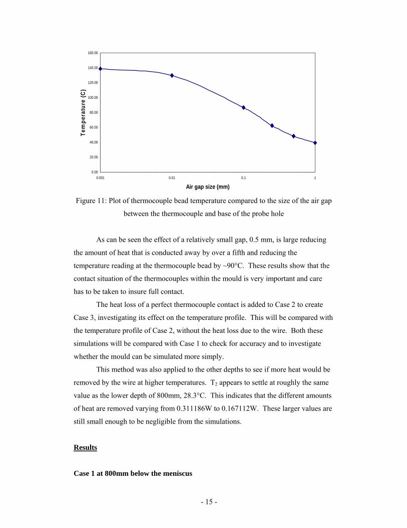
Figure 11: Plot of thermocouple bead temperature compared to the size of the air gap
between the thermocouple and base of the probe hole
As can be seen the effect of a relatively small gap, 0.5 mm, is large reducing
the amount of heat that is conducted away by over a fifth and reducing the
temperature reading at the thermocouple bead by ~90°C. These results show that the
contact situation of the thermocouples within the mould is very important and care
has to be taken to insure full contact.
The heat loss of a perfect thermocouple contact is added to Case 2 to create
Case 3, investigating its effect on the temperature profile. This will be compared with
the temperature profile of Case 2, without the heat loss due to the wire. Both these
simulations will be compared with Case 1 to check for accuracy and to investigate
whether the mould can be simulated more simply.
This method was also applied to the other depths to see if more heat would be
removed by the wire at higher temperatures. T2 appears to settle at roughly the same
value as the lower depth of 800mm, 28.3°C. This indicates that the different amounts
of heat are removed varying from 0.311186W to 0.167112W. These larger values are
still small enough to be negligible from the simulations.
Results
Case 1 at 800mm below the meniscus
- 16 -
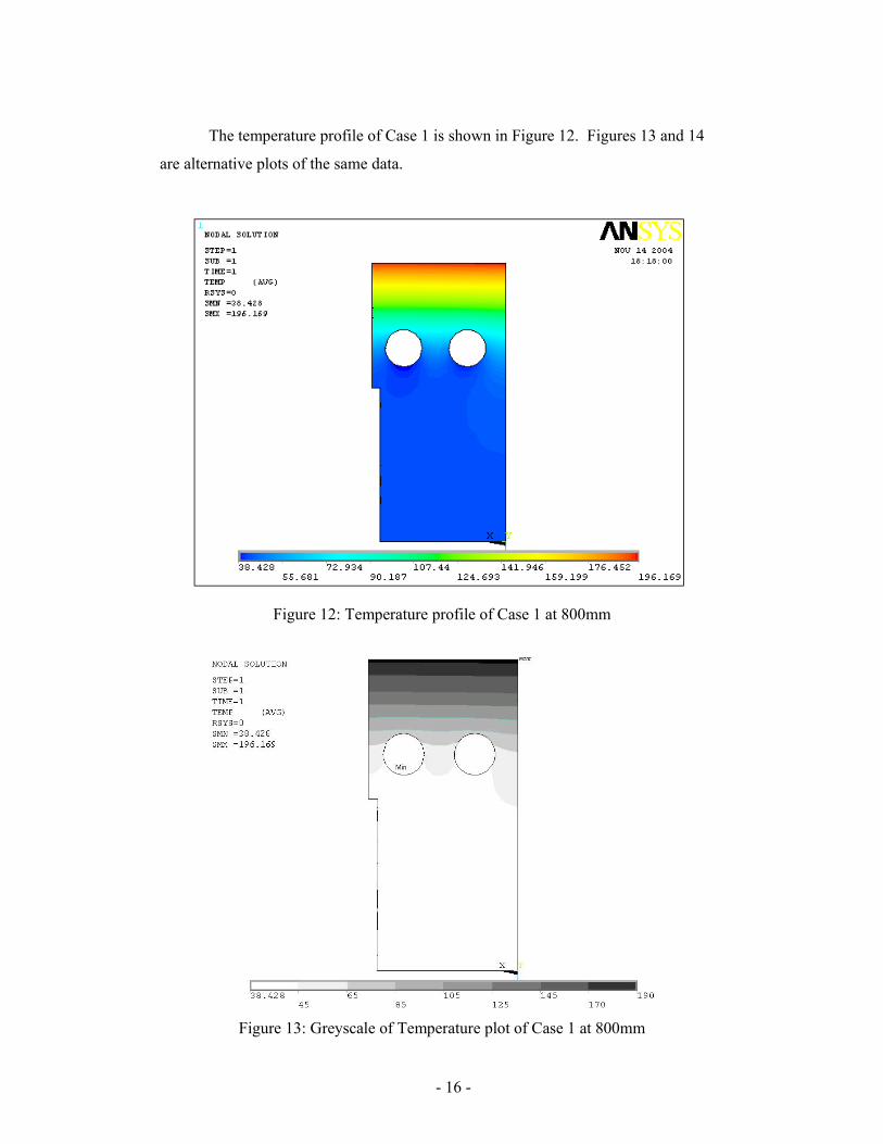
The temperature profile of Case 1 is shown in Figure 12. Figures 13 and 14
are alternative plots of the same data.
Figure 12: Temperature profile of Case 1 at 800mm
Figure 13: Greyscale of Temperature plot of Case 1 at 800mm
- 17 -
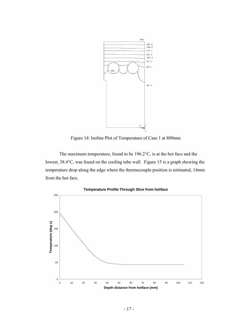
Figure 14: Isoline Plot of Temperature of Case 1 at 800mm
The maximum temperature, found to be 196.2°C, is at the hot face and the
lowest, 38.4°C, was found on the cooling tube wall. Figure 15 is a graph showing the
temperature drop along the edge where the thermocouple position is estimated, 14mm
from the hot face.
Temperature Profile Through Slice from hotface
0
50
100
150
200
250
0 10 20 30 40 50 60 70 80 90 100 110 120
Depth distance from hotface (mm)
Tem
pera
ture
(deg
c)
- 18 -
Figure 15: Temperature drop from hot face
The thermocouple temperature can be interpolated from the data using a linear
method and is found to be 132.7°C. As can be seen the rate of temperature change
reduces greatly once past the cooling tubes at 58mm reaching a reasonably constant
temperature of 43°C.
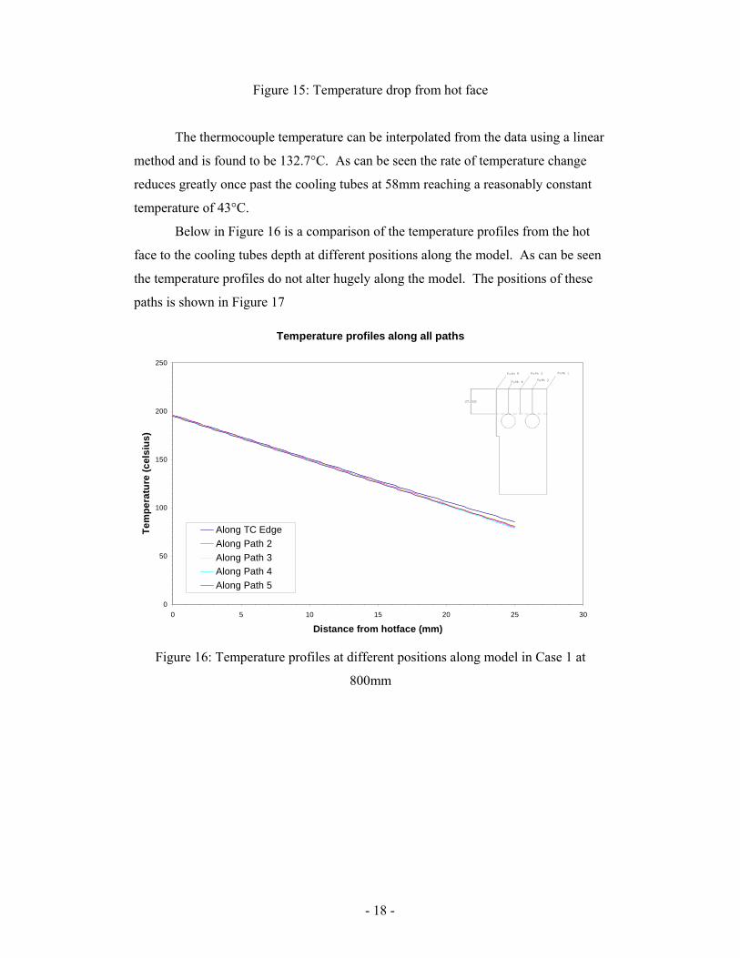
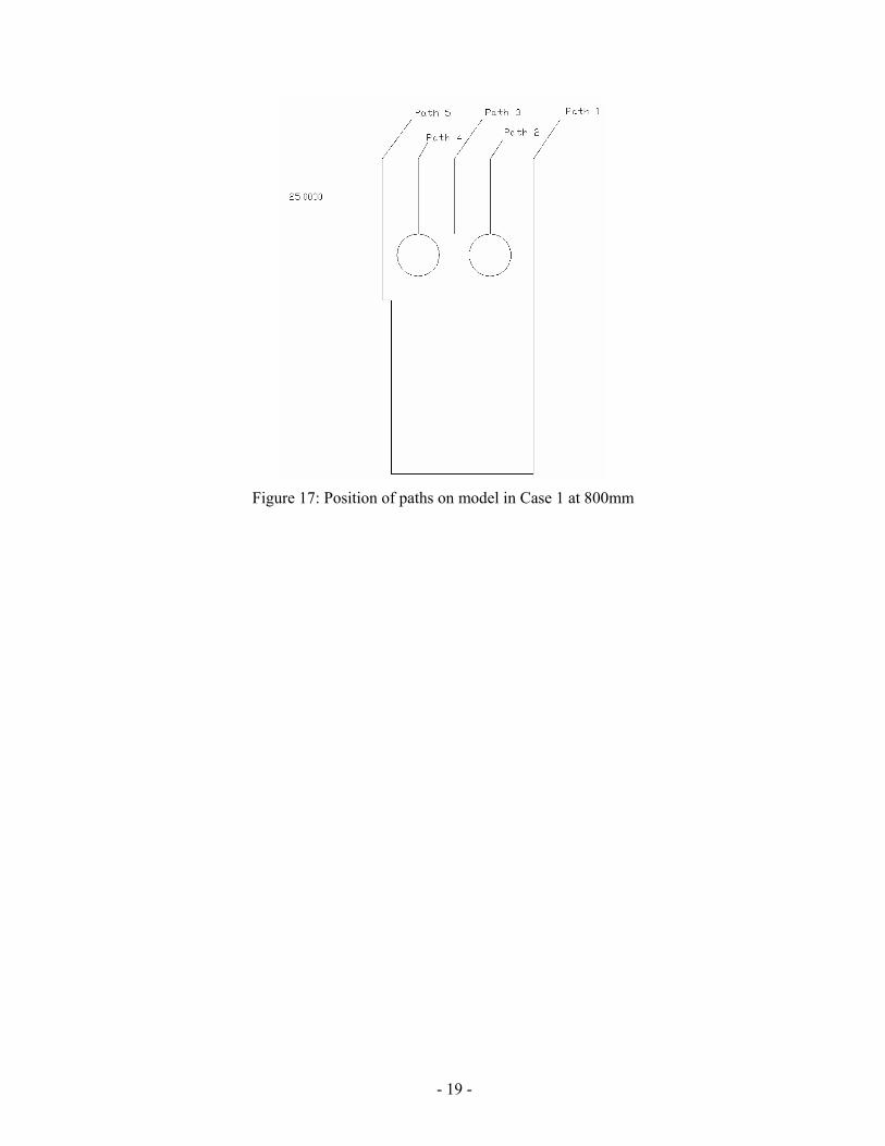
Below in Figure 16 is a comparison of the temperature profiles from the hot
face to the cooling tubes depth at different positions along the model. As can be seen
the temperature profiles do not alter hugely along the model. The positions of these
paths is shown in Figure 17
Temperature profiles along all paths
0
50
100
150
200
250
0 5 10 15 20 25 30
Distance from hotface (mm)
Tem
pera
ture
(cel
sius
)
Along TC EdgeAlong Path 2Along Path 3Along Path 4Along Path 5
Figure 16: Temperature profiles at different positions along model in Case 1 at
800mm
- 19 -
Figure 17: Position of paths on model in Case 1 at 800mm
- 20 -
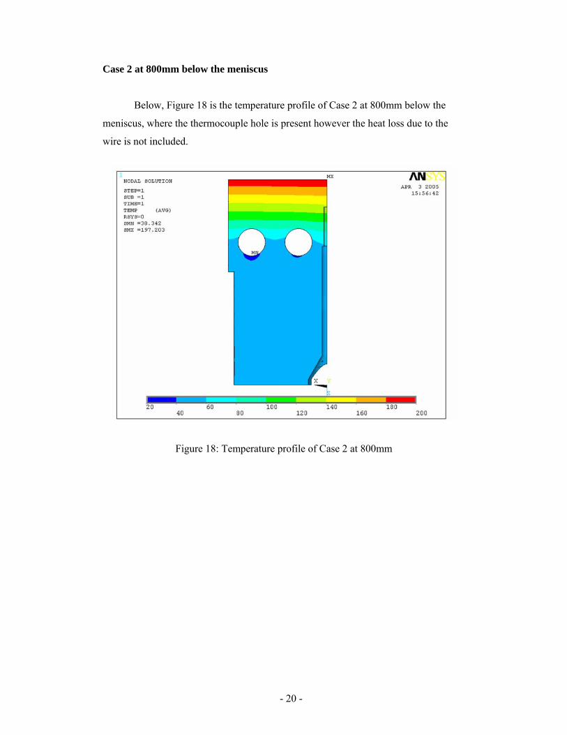
Case 2 at 800mm below the meniscus
Below, Figure 18 is the temperature profile of Case 2 at 800mm below the
meniscus, where the thermocouple hole is present however the heat loss due to the
wire is not included.
Figure 18: Temperature profile of Case 2 at 800mm
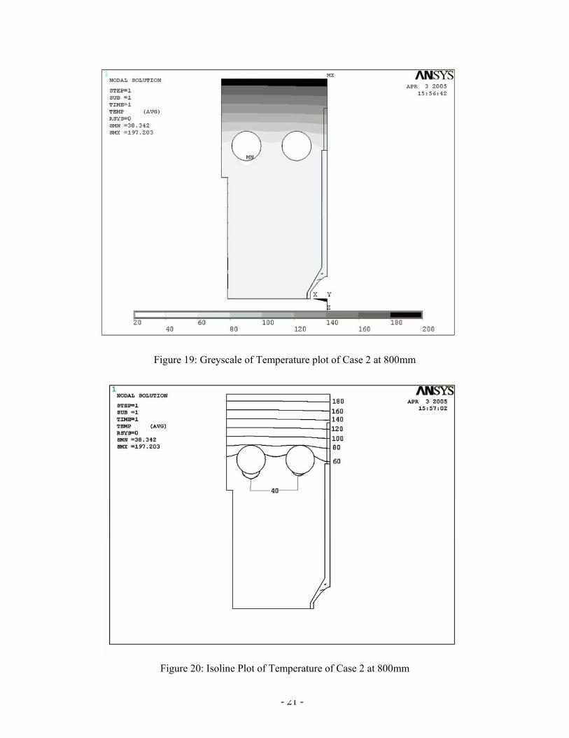
- 21 -
Figure 19: Greyscale of Temperature plot of Case 2 at 800mm
Figure 20: Isoline Plot of Temperature of Case 2 at 800mm
- 22 -
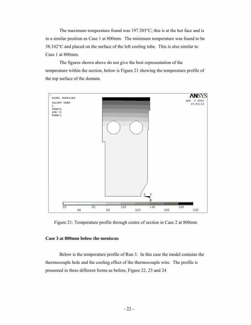
The maximum temperature found was 197.203°C; this is at the hot face and is
in a similar position as Case 1 at 800mm. The minimum temperature was found to be
38.342°C and placed on the surface of the left cooling tube. This is also similar to
Case 1 at 800mm.
The figures shown above do not give the best representation of the
temperature within the section, below is Figure 21 showing the temperature profile of
the top surface of the domain.
Figure 21: Temperature profile through centre of section in Case 2 at 800mm
Case 3 at 800mm below the meniscus
Below is the temperature profile of Run 3. In this case the model contains the
thermocouple hole and the cooling effect of the thermocouple wire. The profile is
presented in three different forms as before, Figure 22, 23 and 24

- 23 -
Figure 22: Temperature profile of Case 3 at 800mm
Figure 23: Greyscale of Temperature plot of Case 3 at 800mm
- 24 -
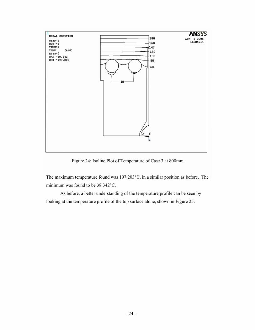
Figure 24: Isoline Plot of Temperature of Case 3 at 800mm
The maximum temperature found was 197.203°C, in a similar position as before. The
minimum was found to be 38.342°C.
As before, a better understanding of the temperature profile can be seen by
looking at the temperature profile of the top surface alone, shown in Figure 25.
- 25 -
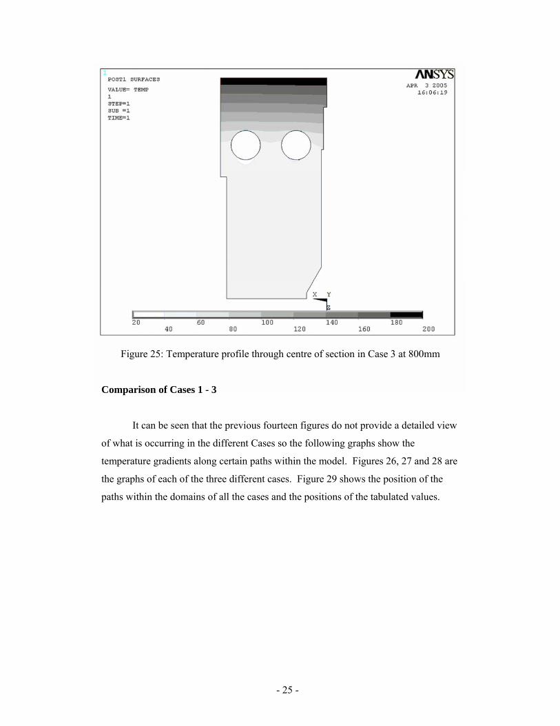
Figure 25: Temperature profile through centre of section in Case 3 at 800mm
Comparison of Cases 1 - 3
It can be seen that the previous fourteen figures do not provide a detailed view
of what is occurring in the different Cases so the following graphs show the
temperature gradients along certain paths within the model. Figures 26, 27 and 28 are
the graphs of each of the three different cases. Figure 29 shows the position of the
paths within the domains of all the cases and the positions of the tabulated values.
- 26 -
Temperature profiles along different paths, no thermocouple hole
0
20
40
60
80
100
120
140
160
180
200
0 20 40 60 80 100
Distance from hotface (mm)
Tem
pera
ture
(C)
Path 1Path 2Path 2Path 3Path 3Path 4
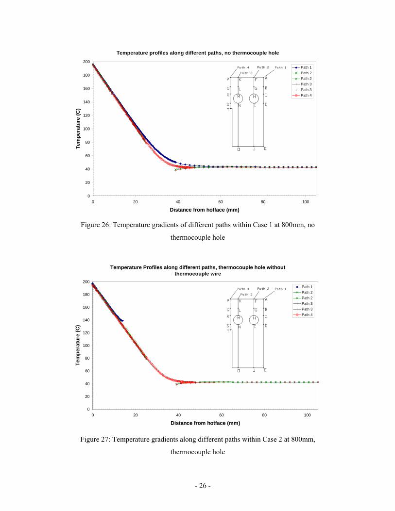
Figure 26: Temperature gradients of different paths within Case 1 at 800mm, no
thermocouple hole
Temperature Profiles along different paths, thermocouple hole without thermocouple wire
0
20
40
60
80
100
120
140
160
180
200
0 20 40 60 80 100
Distance from hotface (mm)
Tem
pera
ture
(C)
Path 1Path 2Path 2Path 3Path 3Path 4
Figure 27: Temperature gradients along different paths within Case 2 at 800mm,
thermocouple hole
- 27 -
Temperature profiles along different paths, thermocouple hole with thermocouple wire
0
20
40
60
80
100
120
140
160
180
200
0 20 40 60 80 100
Distance from hotface (mm)
Tem
pera
ture
(C)
Path 1Path 2Path 2Path 3Path 3Path 4
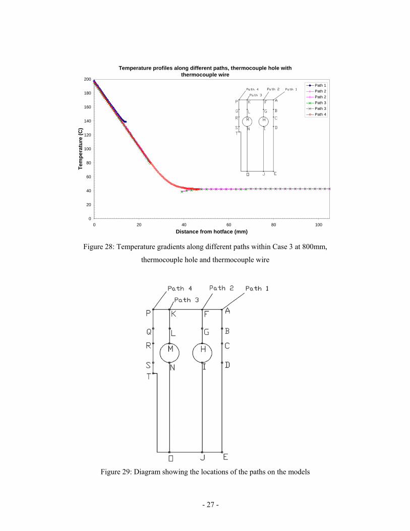
Figure 28: Temperature gradients along different paths within Case 3 at 800mm,
thermocouple hole and thermocouple wire
Figure 29: Diagram showing the locations of the paths on the models

- 28 -
Table 6: Results from key points on Cases 1 – 3 at 800mm
No thermocouple hole
Path 6 Temp Path 4 Temp Path 2 Temp Path 1 Temp P 194.7 K 194.81 F 195.74 A 196.17 Q 130.47 L 130.45 G 131.58 B 132.7 R 80.996 M 78.671 H 79.693 C 85.797 S 44.671 N 38.438 I 39.563 D 50.294 T 42.591 O 43.017 J 43.102 E 43.128
Thermocouple hole no conduction Path 6 Temp Path 4 Temp Path 2 Temp Path 1 Temp P 194.95 K 195.11 F 196.45 A 197.21 Q 130.67 L 130.68 G 132.17 B 138.95 R 81.093 M 78.787 H 79.974 C N/A S 44.589 N 38.345 I 39.299 D N/A T 42.46 O 42.638 J 42.697 E N/A
Thermocouple hole conduction by wire Path 6 Temp Path 4 Temp Path 2 Temp Path 1 Temp P 194.95 K 195.11 F 196.45 A 197.21 Q 130.67 L 130.68 G 132.17 B 138.95 R 81.093 M 78.787 H 79.974 C N/A S 44.589 N 38.345 I 39.299 D N/A T 42.46 O 42.638 J 42.697 E N/A
As can be seen Path 1 in shorter on the last two graphs due to the design of the
domains, the presence of the thermocouple hole cuts the path short at 14mm from the
hot face. This is as expected and allows easy investigation of the temperature at the
bottom of the thermocouple hole. For easier comparison of the three simulations
below in Figure 30 is a graph showing the temperature gradients of Path 1 of all the
three cases.
- 29 -
Temperature along thermocouple edge of the all three situations
0
20
40
60
80
100
120
140
160
180
200
0 20 40 60 80 100
Distance from hotface (mm)
Tem
pera
ture
(C)
Hole, no wireHole with wireNo Hole
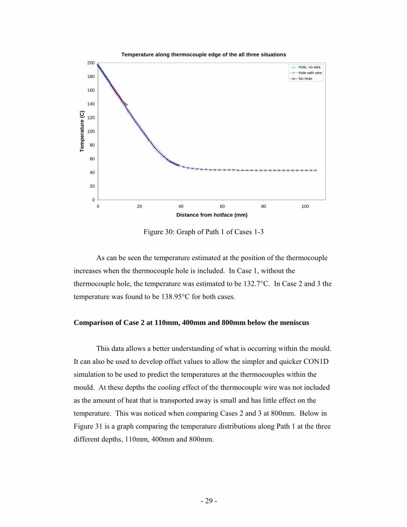
Figure 30: Graph of Path 1 of Cases 1-3
As can be seen the temperature estimated at the position of the thermocouple
increases when the thermocouple hole is included. In Case 1, without the
thermocouple hole, the temperature was estimated to be 132.7°C. In Case 2 and 3 the
temperature was found to be 138.95°C for both cases.
Comparison of Case 2 at 110mm, 400mm and 800mm below the meniscus
This data allows a better understanding of what is occurring within the mould.
It can also be used to develop offset values to allow the simpler and quicker CON1D
simulation to be used to predict the temperatures at the thermocouples within the
mould. At these depths the cooling effect of the thermocouple wire was not included
as the amount of heat that is transported away is small and has little effect on the
temperature. This was noticed when comparing Cases 2 and 3 at 800mm. Below in
Figure 31 is a graph comparing the temperature distributions along Path 1 at the three
different depths, 110mm, 400mm and 800mm.

- 30 -
Comparison of Temperature profiles from hotface to base of thermocouple hole at different depths
0
50
100
150
200
250
300
350
0 1 2 3 4 5 6 7 8 9 10 11 12 13 14 15
Distance from hotface (mm)
Tem
pera
ture
(C)
110mm below meniscus400mm below meniscus800mm below meniscus
Figure 31: Comparison of Path 1 temperature distributions at different depths (Case 2)
It can be seen that the distributions are similar though as the depth decreases
the temperatures obviously increase and the gradients increase due to larger
temperature differences between the hot face and the cooling tubes. The temperatures
at the base of the thermocouple hole was found to be 234.43°C at 110mm, 169.34°C
at 400mm and 139.95°C at 800mm. The maximum hot face temperatures were found
to be 343.18°C, 244.6°C and 197.20°C at 110mm, 400mm and 800mm respectively.
In Figure 32 a plot of heat flux against temperature of the hot face is shown.
This shows that there is a linear correlation and allows an estimation of hot face
temperature if the heat flux can be found or vice-a-versa.

- 31 -
Comparison of heat flux against temperature of hotface
150
170
190
210
230
250
270
290
310
330
350
1.50E+06 2.00E+06 2.50E+06 3.00E+06 3.50E+06
Heat flux (W)
Tem
pera
ture
(C)
150
170
190
210
230
250
270
290
310
330
350
Max temperature measured on hotface
Min temperature measured on hotface
Linear (Min temperature measured on hotface)
Linear (Max temperature measured on hotface)
Figure 32: Plot of heat flux from the molten steel compared to hot face temperature
(Case 2 domains)
Comparison of Case 2 and Case 4
The data for Case 4 was compared to Case 2 as both these situations do not
contain the thermocouple cooling effect. From the data shown in Figure 33 is a plot
along path 1 on the mould, the path from the hot face to the base of the thermocouple
hole.
- 32 -
Comparison of Case 2 and Case 4
120
130
140
150
160
170
180
190
200
0 1 2 3 4 5 6 7 8 9 10 11 12 13 14 15
Distance from hot face (mm)
Tem
pera
ture
(C)
Case 2 - Full size domainwith thermocouple hole
Case 4 - Shorter domainwith thermocouple hole
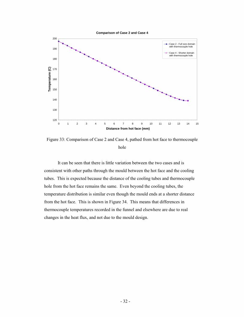
Figure 33: Comparison of Case 2 and Case 4, pathed from hot face to thermocouple
hole
It can be seen that there is little variation between the two cases and is
consistent with other paths through the mould between the hot face and the cooling
tubes. This is expected because the distance of the cooling tubes and thermocouple
hole from the hot face remains the same. Even beyond the cooling tubes, the
temperature distribution is similar even though the mould ends at a shorter distance
from the hot face. This is shown in Figure 34. This means that differences in
thermocouple temperatures recorded in the funnel and elsewhere are due to real
changes in the heat flux, and not due to the mould design.
- 33 -
Comparison of Case 2 and Case 4
0
20
40
60
80
100
120
140
160
180
200
0 20 40 60 80 100
Distance from hot face (mm)
Tem
pera
ture
(C)
Case 2 - Full size domain - path 2Case 2 - Full size domain - path 2Case 4 - Shorter domain - path 2Case 4 - Shorter domain - path 2
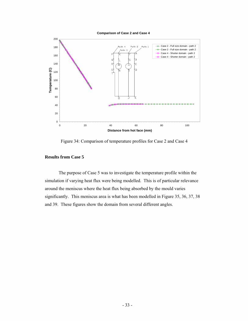
Figure 34: Comparison of temperature profiles for Case 2 and Case 4
Results from Case 5
The purpose of Case 5 was to investigate the temperature profile within the
simulation if varying heat flux were being modelled. This is of particular relevance
around the meniscus where the heat flux being absorbed by the mould varies
significantly. This meniscus area is what has been modelled in Figure 35, 36, 37, 38
and 39. These figures show the domain from several different angles.

- 34 -
Figure 35: Colour plot of the Case 5 domain showing the temperature profile around
the meniscus
Figure 36: Black and white plot of the Case 5 domain showing the temperature profile
around the meniscus
- 35 -
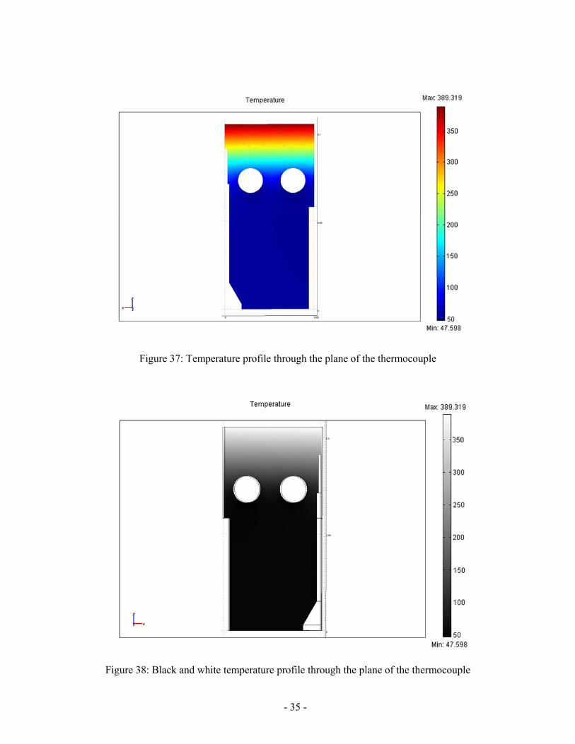
Figure 37: Temperature profile through the plane of the thermocouple
Figure 38: Black and white temperature profile through the plane of the thermocouple

- 36 -
Figure 39: Temperature profile along the thermocouple side of the domain.
As can be seen from these plots the varying heat flux alters the temperature
profile as expected though not in any unusual ways. These plots cannot be compared
to previous cases as the domain is significantly different however the boundary
conditions can be altered so that the thermocouple is placed in the same position as
the previous cases. This allows the simulation to be verified and found to be
reasonably accurate.
The maximum thermocouple temperatures were found to be 233.3°C, 168.8°C
and 136.5°C for the analysed depths of 110mm, 400mm and 800mm below the
meniscus. When these are compared to the previous temperatures found of 234.43°C
at 110mm, 169.34°C at 400mm and 139.95°C at 800mm it can be seen that there is at
least 0.54°C difference though the maximum difference is 3.45°C. This is likely due
to an average value being used for the convection coefficient and water temperature in
the cooling tubes. Ideally using a similar interpolation method on the tubes as the hot
face would have been better but due program errors this was not currently possible but
could be achieved in the future.
- 37 -
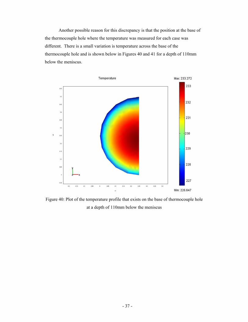
Another possible reason for this discrepancy is that the position at the base of
the thermocouple hole where the temperature was measured for each case was
different. There is a small variation is temperature across the base of the
thermocouple hole and is shown below in Figures 40 and 41 for a depth of 110mm
below the meniscus.
Figure 40: Plot of the temperature profile that exists on the base of thermocouple hole
at a depth of 110mm below the meniscus
- 38 -
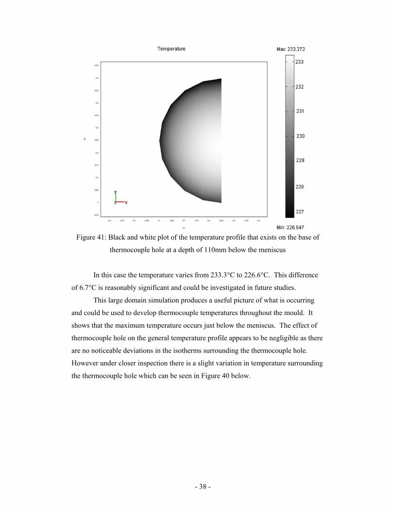
Figure 41: Black and white plot of the temperature profile that exists on the base of
thermocouple hole at a depth of 110mm below the meniscus
In this case the temperature varies from 233.3°C to 226.6°C. This difference
of 6.7°C is reasonably significant and could be investigated in future studies.
This large domain simulation produces a useful picture of what is occurring
and could be used to develop thermocouple temperatures throughout the mould. It
shows that the maximum temperature occurs just below the meniscus. The effect of
thermocouple hole on the general temperature profile appears to be negligible as there
are no noticeable deviations in the isotherms surrounding the thermocouple hole.
However under closer inspection there is a slight variation in temperature surrounding
the thermocouple hole which can be seen in Figure 40 below.
- 39 -
Profiles of tem perature and heat flux along length of dom ain
0
1000000
2000000
3000000
4000000
5000000
-0.02 0 0.02 0.04 0.06 0.08 0.1 0.12 0.14
Distance from m eniscus (m )
Hea
t flu
x (W
/m^2
)
0
50
100
150
200
250
300
350
400
450
Tem
pera
ture
(deg
C)
FEMLAB interpolated heat flux
CON1D Heat flux
Temperature at depth of TC, 14mm from hotface
Temperature at surface
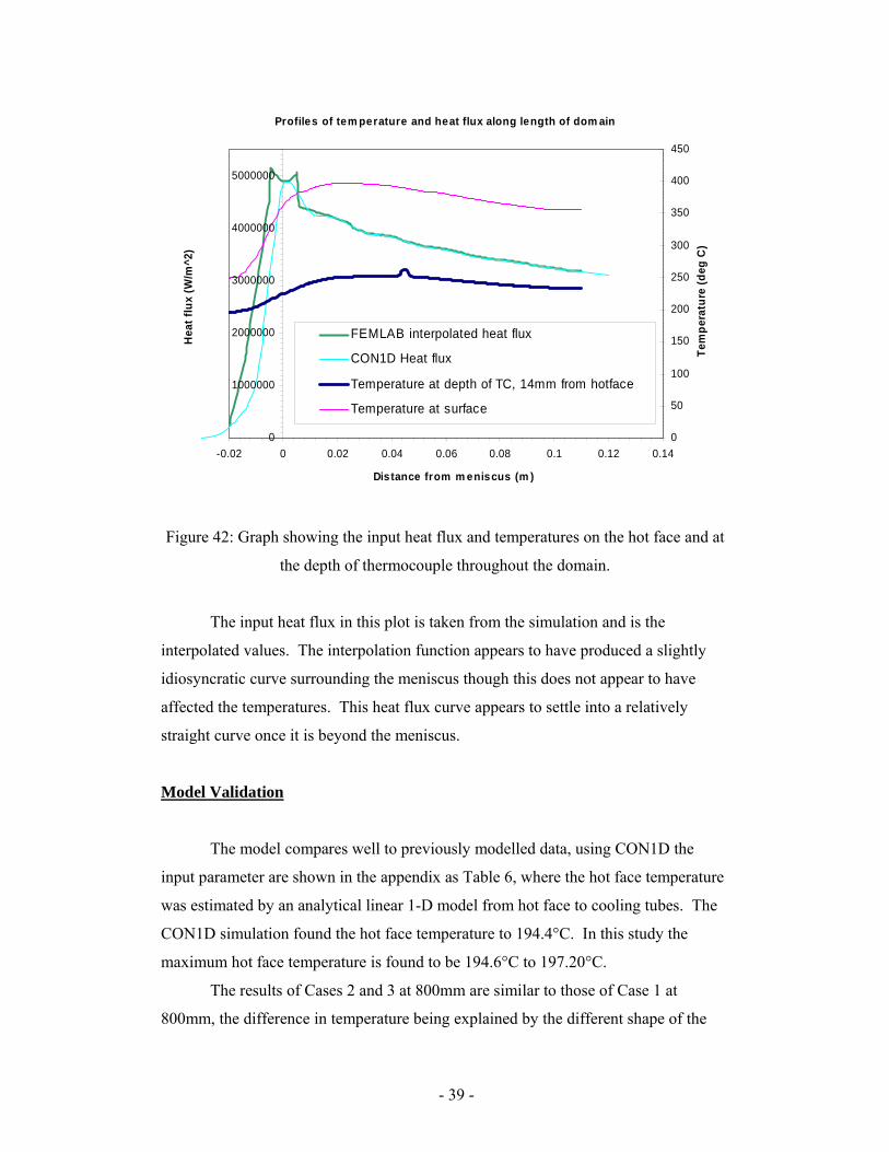
Figure 42: Graph showing the input heat flux and temperatures on the hot face and at
the depth of thermocouple throughout the domain.
The input heat flux in this plot is taken from the simulation and is the
interpolated values. The interpolation function appears to have produced a slightly
idiosyncratic curve surrounding the meniscus though this does not appear to have
affected the temperatures. This heat flux curve appears to settle into a relatively
straight curve once it is beyond the meniscus.
Model Validation
The model compares well to previously modelled data, using CON1D the
input parameter are shown in the appendix as Table 6, where the hot face temperature
was estimated by an analytical linear 1-D model from hot face to cooling tubes. The
CON1D simulation found the hot face temperature to 194.4°C. In this study the
maximum hot face temperature is found to be 194.6°C to 197.20°C.
The results of Cases 2 and 3 at 800mm are similar to those of Case 1 at
800mm, the difference in temperature being explained by the different shape of the

- 40 -
domains used. The new domain has less material to absorb the heat from the hot face
creating slightly hotter temperatures. In Case 3 at 800mm the hot face temperature
was found to be 194.95°C to 197.20°C. The data developed for Case 2 at 110mm and
400mm appear to agree with the CON1D data like the previous Cases.
Case 5 was compared with previous cases by simulating the domain at the
specific depths. As was mentioned above there is a variation in the thermocouple
temperatures between the cases however this can be attributed to several possible
factors.
CON1D Calibration
Boundary conditions: Properties and conditions
ANSYS CON1D
Thermal conductivity of copper (W m-1K-1)
372 372
Distance of thermocouple from hot face (mm)
14 14 or 12.2
Remaining faces of model
Perfectly insulated Perfectly insulated
Water Velocity in bored holes (m/s)
8.7 8.7
Conditions at individual depths below meniscus
110 (ANSYS|CON1D)
400 (ANSYS|CON1D)
800 (ANSYS|CON1D)
Heat Flux (MW m-2) 3.18 3.18 2.201 2.201 1.704 1.704 Water tube heat transfer coefficient (kW m-2K-2) 32.4412 * 34.6691 * 35.7748 * Water temperature (°C) 21.31 * 25.00 * 28.31 * * based on Sleicher and Rouse Equation ANSYS Case:
- 41 -
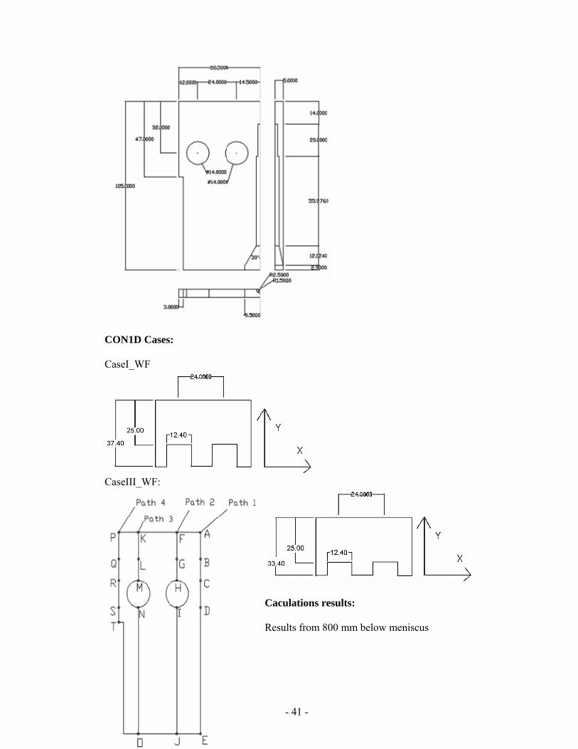
CON1D Cases: CaseI_WF
CaseIII_WF:
Caculations results: Results from 800 mm below meniscus
- 42 -
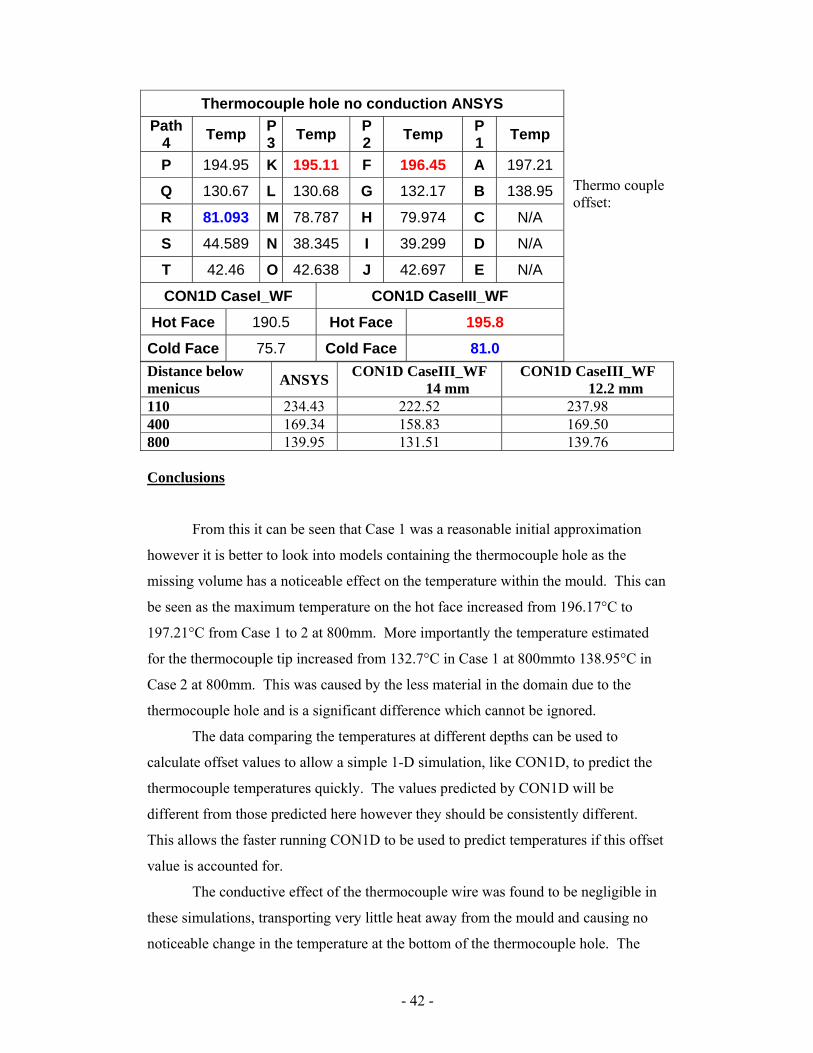
Thermo couple offset:
Distance below menicus ANSYS CON1D CaseIII_WF
14 mm CON1D CaseIII_WF
12.2 mm 110 234.43 222.52 237.98 400 169.34 158.83 169.50 800 139.95 131.51 139.76 Conclusions
From this it can be seen that Case 1 was a reasonable initial approximation
however it is better to look into models containing the thermocouple hole as the
missing volume has a noticeable effect on the temperature within the mould. This can
be seen as the maximum temperature on the hot face increased from 196.17°C to
197.21°C from Case 1 to 2 at 800mm. More importantly the temperature estimated
for the thermocouple tip increased from 132.7°C in Case 1 at 800mmto 138.95°C in
Case 2 at 800mm. This was caused by the less material in the domain due to the
thermocouple hole and is a significant difference which cannot be ignored.
The data comparing the temperatures at different depths can be used to
calculate offset values to allow a simple 1-D simulation, like CON1D, to predict the
thermocouple temperatures quickly. The values predicted by CON1D will be
different from those predicted here however they should be consistently different.
This allows the faster running CON1D to be used to predict temperatures if this offset
value is accounted for.
The conductive effect of the thermocouple wire was found to be negligible in
these simulations, transporting very little heat away from the mould and causing no
noticeable change in the temperature at the bottom of the thermocouple hole. The
Thermocouple hole no conduction ANSYS Path
4 Temp P3 Temp P
2 Temp P 1 Temp
P 194.95 K 195.11 F 196.45 A 197.21
Q 130.67 L 130.68 G 132.17 B 138.95
R 81.093 M 78.787 H 79.974 C N/A
S 44.589 N 38.345 I 39.299 D N/A
T 42.46 O 42.638 J 42.697 E N/A
CON1D CaseI_WF CON1D CaseIII_WF
Hot Face 190.5 Hot Face 195.8
Cold Face 75.7 Cold Face 81.0

- 43 -
investigation into effect of air gaps at the thermocouple bead found that this additional
thermal resistance can significantly affect the amount of heat transported away by the
wire. The heat transported away is reduced further showing that the cooling effect of
the thermocouple wires can be neglected. The more important result is the reduction
of the temperature present at the thermocouple bead; this shows that the presence of a
small air gap can cause a large error in measured temperatures.
The effect of the mould beyond the cooling tubes is found to negligible with
no affect on the thermocouple temperature or on the temperature distribution within
the mould. This allows a single model to be used for both the funnelled section and
the mould edge.
The varying heat flux does cause gross temperature changes within the mould
which is as expected. This temperature variation is reasonably linear within the
mould at specific distances from the hot face. This linearity breaks down around the
meniscus. This section has a rapidly changing heat flux causing rapid temperature
rise within the mould making temperature readings within this section to be very
sensitive to position. It is recommended to take measurements from a depth below
the meniscus and interpolate the hot face temperature around the meniscus from these
readings.
These Cases appear to be good estimations of the actual mould. It would be
best to conduct parametric studies now to investigate whether this method is
reasonable when applied generally. The parametric studies could cover the effect of
thermocouple hole size, cooling tube position and size. The meniscus region is the
most critical as the most wear occurs here. Further investigation is required to
understand more fully the damage effects occurring here.
Finally, CON1D has been calibrated to match the 3-D finite-element model
predictions, so long as the mold thickness input to CON1D is fixed at 33.4mm
(instead of a range of thicknesses around the of funnel up to 105mm).
The CON1D prediction of thermocouple temperatures is accurate, so long as the
thermocouple distance below the hotface is offset by 1.8mm (meaning that TCs in
CON1D should positioned at 12.2 mm below the hotface, which is 1.8mm closer to
the hotface than actually occurs in the caster).

- 44 -
Appendix
Table 7: Standard Input Conditions for CON1D simulation Carbon Content, C% 0.03 % Liquidus Temperature, Tliq 1529 oC Solidus Temperature, Tsol 1509 oC Steel Density, ρsteel 7400 kg/m2
Steel Emissivity, εsteel 0.8 - Fraction Solid for Shell Thickness Location, fs 0.7 - Mould Thickness at Top (Outer face, including water channel) 37.4 mm Mould Outer Face Radius, Ro 0 m Total Mould Length, Zmold_total 1100 mm Total Mould Width 1876 mm Scale thickness at mould cold face (inserts region/ below), dscale 0.02/0.01 mm Initial Cooling Water Temperature, Twater 20 oC
Water Channel Geometry, ch ch chd w L× × 244.124.12 ×× mm3
Cooling Water Velocity, Vwater 8.7 m/s Mould Conductivity, kmold 360 W/mK Mould Emissivity, εmould 0.5 - Mould Powder Solidification Temperature, Tfsol 1045 oC Mould Powder Conductivity, ksolid/kliquid 1.5/1.5 W/mK Air Conductivity, kair 0.0599 W/mK Slag Layer/Mould Resistance, rcontact 5.0E-9 m2K/W
Mould Powder Viscosity at 1300oC, 1300µ 1.2 Poise
Exponent for Temperature dependence of Viscosity, n 0.85 - Slag Density, ρslag 2500 kg/m3 Slag Absorption Factor, a 250 m-1 Slag Refractive Index, m 1.5 - Slag Emissivity, εslag 0.9 - Mould Powder Consumption Rate, Qslag 0.12 kg/m2
Empirical solid slag layer speed factor, fv 0.175 - Casting Speed, Vc 3.6 m/min Pour Temperature, Tpour 1550 oC Slab Geometry, W N× 1450×90 mm×mm Nozzle Submergence Depth, dnozzle 265 mm Working Mould Length, Zmold 1100 mm
Oscillation Mark Geometry, mark markd w× 11.0 × mm×mm
Mould Oscillation Frequency, freq 4.67 cpm Oscillation Stroke, stroke 6 mm Time Step, dt 0.002 s Mesh Size, dx 0.5 mm

- 45 -
References
1. Metallurgical and Materials Transactions B, Vol. 34B, No. 5, Oct., 2003, pp. 685-705.
2. www.ansys.com
3. www.comsol.com
Simulation Conditions Thermal conductivity of copper 372 W m-1K-1 Distance of thermocouple from hot face 14mm Remaining faces of model Perfectly insulated Water Velocity in bored holes 8.7 m/s Depth below meniscus (mm) 800 Heat Flux (MW m-2) 1.704 Water tube heat transfer coefficient (kW m-2K-2) 35.7748 Water temperature (°C) 28.31