A User’s Guide tothe STRAINS program

(Version 1.0 for IBM PC & Compatibles)

J.S. Sharma

CUED/D-Soils/TR280 January 1995

Disclaimer: Anyone using the computer programs described in this guide may doso entirely at his/her own risk. Whilst every effort has been made to ensure theircorrectness and this disclaimer is not intended to discourage their use, the user isstrongly recommended to critically examine the results and consider whether the useof the program is appropriate. The author of the program and the CambridgeUniversity Engineering Department are not responsible for any loss or damagewhatsoever arising from errors, if any, in the programs or erroneous interpretationof the results produced by the program.

Contents

CONTENTS . . . . . . . . . . . . . . . . . . . . . . . . . . . . . . . . . . . . . . . . . . . . . . . . . . . . . . . . . . . . . . . . . . . . . . . . . . . . . . . . . . . . . . . . . . . . . . . . . . . . . . . . . . . . . . . . . . . . . . . . ............................ 2

1. INTRODUCTION .................................................................................................................................. . . . . 3

1.1 HLWORY.. ................................................................................................................................................... 3

1.2 STRAMj FOR IBM PC 8~ COMPATIELES .................................................................................................... 41.3 CA~ABILITIESOFTHEIBMPCVERSIONOFTHES’IRA~NSPROGRAM.. ........................................................ .5

2. FILM MEASUREMENT........................................................................................................................... 6

2.1 THEFILMMEASUREMENTMACHINE(FMM). .............................................................................................. .62.2 FILMMEASUREMENT.. ................................................................................................................................. 6

3. THE STRAINS PROGRAM ......................................................................................................... . ............ 8

3.1 ANOVERVIEW.. .......................................................................................................................................... 83.2 HARDWARE AND SOFTWARE REQUIREMENTS.. ............................................................................................. .83.3 INSTALLATION OF STRAINS ...................................................................................................................... .83.4 RUNNING THE STRAINS PROGRAM ............................................................................................................ .9

3.4.1 File Handling Strategy ...................................................................................................................... .9

3.4.2 Various Menus in STRAINS .............................................................................................................. Zl

APPENDIX A: THE CALCULATION OF STRAINS ................. . ............................................................. 20

A. 1 INTRODUCTION ....................................................................................................................................... .2O

A.2 ASSLM~IIONS .......................................................................................................................................... 21A.3 THE TRANSFORMATION OF CO-ORDINATES ................................................................................................ 22A.4 CALfJJLATION OF DISPLACEMENTS AND STRAINS........................................................................................ 23

A.4.1 Plane strain ..................................................................................................................................... 24A.4.2 Axisymmetric strain ......................................................................................................................... 26

APPENDIX B: EDITING THE PLOT FILES USING LOTUS FREELANCE......................................... 27

B 1 INTRODUC~ON ......................................................................................................................................... 27.B.2 I~GQRTING THE PLOT FILE INTO LoTus FREELANCE .................................................................................... 27B.3 EDITINGTHEIMPORTEDPLOTFILE.. .......................................................................................................... .28

REFERENCES .............................................................................................................................................. 29

1. Introduction

1.1 History

The method of determining strains in soils by radiography was first developed at

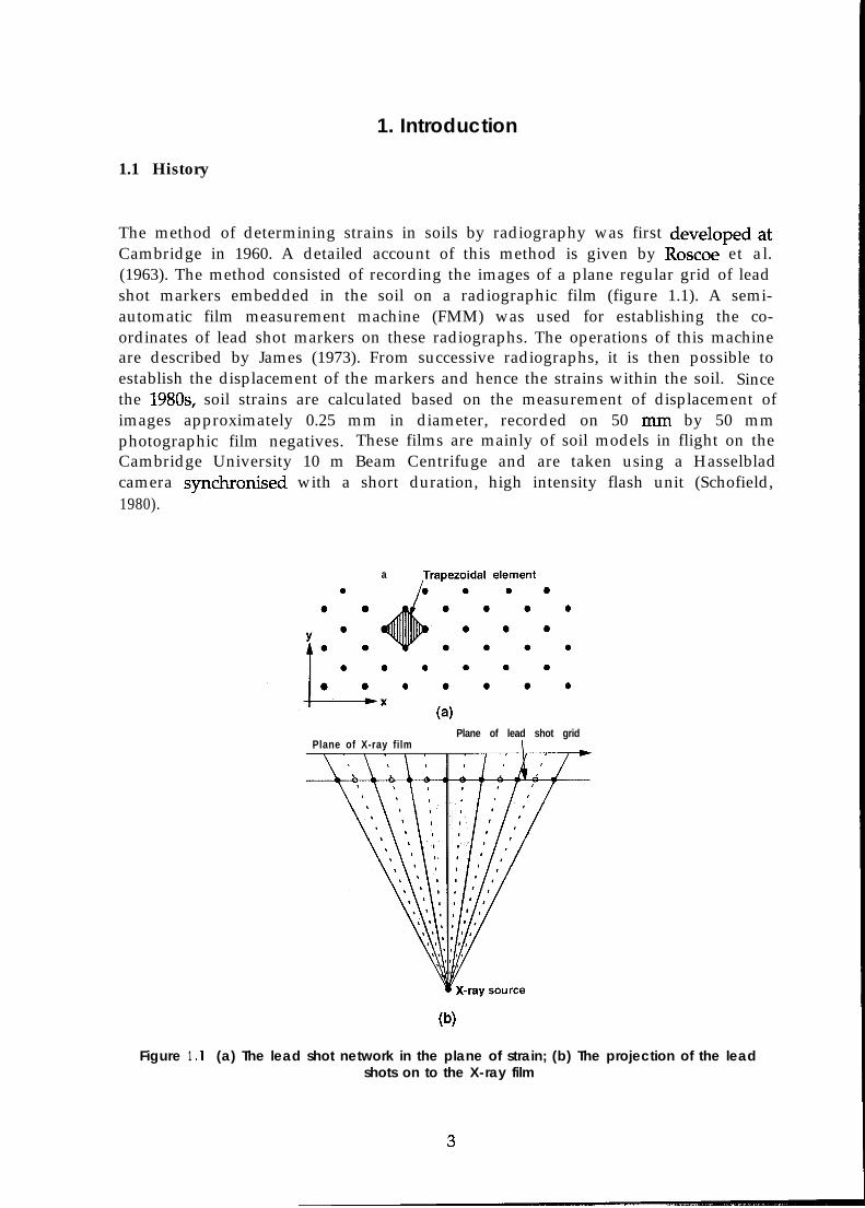
Cambridge in 1960. A detailed account of this method is given by Roscoe et al.(1963). The method consisted of recording the images of a plane regular grid of leadshot markers embedded in the soil on a radiographic film (figure 1.1). A semi-automatic film measurement machine (FMM) was used for establishing the co-ordinates of lead shot markers on these radiographs. The operations of this machineare described by James (1973). From successive radiographs, it is then possible toestablish the displacement of the markers and hence the strains within the soil. Sincethe 198Os, soil strains are calculated based on the measurement of displacement ofimages approximately 0.25 mm in diameter, recorded on 50 nun by 50 mmphotographic film negatives. These films are mainly of soil models in flight on theCambridge University 10 m Beam Centrifuge and are taken using a Hasselbladcamera synchronised with a short duration, high intensity flash unit (Schofield,1980).

Figure 1

0

a ,Fpez;dal ellment a

Plane of X-ray filmPlane of lead shot grid

1

W

.l (a) The lead shot network in the plane of strain; (b) The projection of the leadshots on to the X-ray film

The computer code for calculating soil strains called “STRAINS”, based on thedisplacement of markers, was first written by Orr in 1974 and was mounted on anIBM 370 mainframe computer. It was later modified by Britto in 1980 and wasmounted on an IBM 3081 mainframe computer. The last modification to theSTRAINS program was carried out by Britto in 1984. The program still exists on theIBM 3081 and is specified in its user’s guide (Britto, 1984).

1.2 STRAINS for IBM PC & Compatibles

Although the STRAINS program can be run on the IBM 3081 computer, it has fourmajor drawbacks:

(1) The user has to get familiar with the Job Command Language (JCL) of the IBM3081 computer because the only way the program can be run is in thebackground mode using submission of a job.

(2) The plot files are generated using the CAMPLOT graphics library which waswritten and developed at the Computer Laboratories of Cambridge Universityand is unique to the IBM 3081 computer. Therefore, they can not easily beimported into any other computer (for editing using any standard graphicssoftware, for example). Also, with the advent of sophisticated word processingsoftwares, the present day user demands direct incorporation of graphs,diagrams, etc. into his document. This is almost impossible to achieve usingthe plot files written in CAMPLOT format.

(3) Hardcopies of the plots can only be obtained using the flatbed plotters locatedin the Computing Laboratories. These plotters use a 300 nun wide roll ofpaper. A job should be submitted to the operators requesting for hardcopies ofthe plots. The user has no control over the quality of these plots. Also, theplots can not be print-previewed before sending the request for hardcopies.There is an alternative way of obtaining hardcopies of the plots. It involvescreating postscript files of the plots using the program PLTOPS (resident onlyon IBM 3081), downloading these postscript files onto a floppy disk using anyfile transfer program (usually FTP) and printing them on a postscript laserprinter. Both these ways are obviously cumbersome.

(4) The mainframe version of STRAINS program does not generate any contourplots (for example, shear strain contours).

With the objective of obviating the above-mentioned drawbacks, it was decided todevelop a new version of the STRAINS program. The fact that the IBM 3081computer will be decommissioned by September 1995 contributed towards theurgency to develop the new version. It was decided to develop the new version onan IBM PC platform because now-a-days it is the most-used type of personalcomputer.

4

1.3 Capabilities of the IBM PC Version of the STRAINS Program

Version 1.0 of the STRAINS program is capable of producing basic strains data fromraw unedited FMM data and displaying and plotting them suitably. At present, it issuitable only for regularly spaced rectangular grid of markers. No exact informationis required about the number of rows (should be less than 36) of markers on a film,or the number of markers in a row (should be between 5 and 49). Should up to 10consecutive markers be missing when measuring a film, the program willautomatically insert markers as required. The data for duplicated markers areaveraged. No data are plotted or printed for the inserted shots. The markers areautomatically aligned using a least square method on each film and between films,to give a characteristic row and column number to each shot. All the strains arecalculated based on the method described in Appendix A. The program generatesplot files of the following parameters:

1. Zero extension line direction2. Direction of largest compressive strain3. Magnitude and direction of principal strains4. Displacement of markers5. Centre of gravity of each triangle formed by three markers

In addition, the program can produce contour plots of the following parameters:

1. Horizontal displacement2. Vertical displacement3. Shear strain4. Volumetric strain5. Angle of dilation

These plots can be viewed and print-previewed on either a standard VGA monitoror a high resolution SVGA monitor. Hardcopies of these plots are in the HP-GL(Hewlett-Packard Graphics Language) format. The HP-GL format allows the importof these plots into any graphics editor such as Lotus Freelance for Windows (seeAppendix B) or into any word processor such as Microsoft Word for Windows.Since the program is compiled using the Salford University FTN77 compiler, itrequires a run-time system (called DBOS) to be present on the computer for itsexecution.

5

2. Film Measurement

2.1 The Film Measurement Machine (FMM)

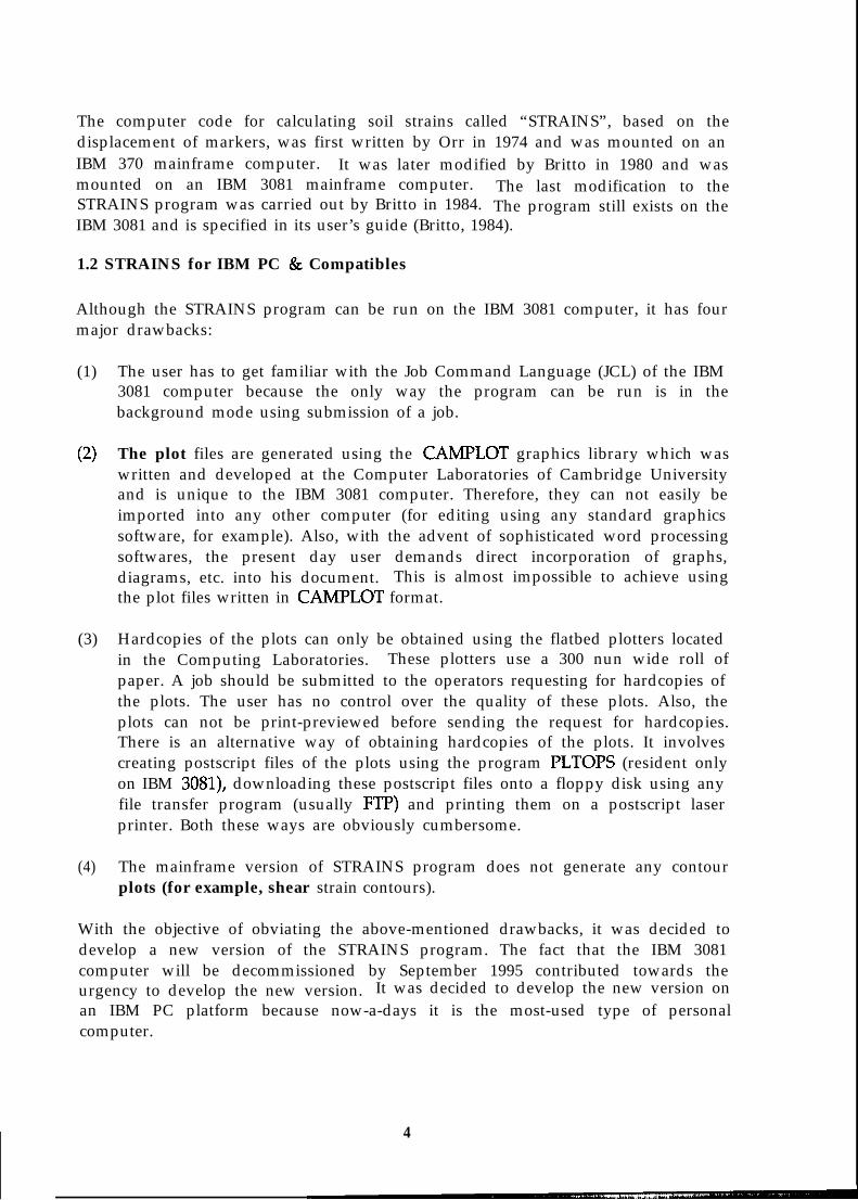
The design and operations of the FMM have been described in detail by Phillips(1991) and hence, only a brief description is provided here. The FMM comprises of afilm carriage, a moire fringe co-ordinate measuring system and a 286 PC computer(figure 2.1). All controls are performed via the computer using a computer programwritten in Microsoft Quickbasic version 4.0. The accuracy of the FMM is about tiurn which is limited only by the CCTV system. At the end of the measurement of afilm, an output file is created which contains the co-ordinates of the markers. Thisoutput file is then processed using the STRAINS program.

LEGEND :A - Projector Illumination SourceB - Cooling FanC - Film CarriageD - FilmE - Linear EncoderF - Zoom LensG - Half-silvered MirrorH - TV CameraI - Video OverlayJ - TV MonitorK - PC 266 ComputerL - Observation ScreenM - X-Drive Stepper MotorN - Y-Drive Stepper Motor

Figure 2.1 Schematic diagram of the Film Measurement Machine (FMM)

2.2 Film Measurement

Each film should have at least two reference markers on it. Two fixed markers,attached to the outside of the apparatus but inside the field view of the film, aresuggested. The co-ordinates of these reference markers, (xl, yl) and (~2, y2), must beknown with respect to a real space axis which must be chosen so that all of themarkers in the grid lie in the first quadrant. Also, in the case of axisymmetric strainfield, the user is advised to have two more reference markers defining the axis ofsymmetry. It is necessary to use a right-handed co-ordinate system with the x-axishorizontal and the y-axis vertical. Each row should have a nominally constant yvalue. The film should be placed on the FMM in such a way that the view as seen onthe screen is the same as the view of the apparatus from the camera side and is thecorrect way up. It is not necessary to place all films on the carriage in exactly the

6

same position. However, it is recommended that the films are placed atapproximately the same position in order to avoid the errors in measurement due tooptical non-linearity of the FMM.

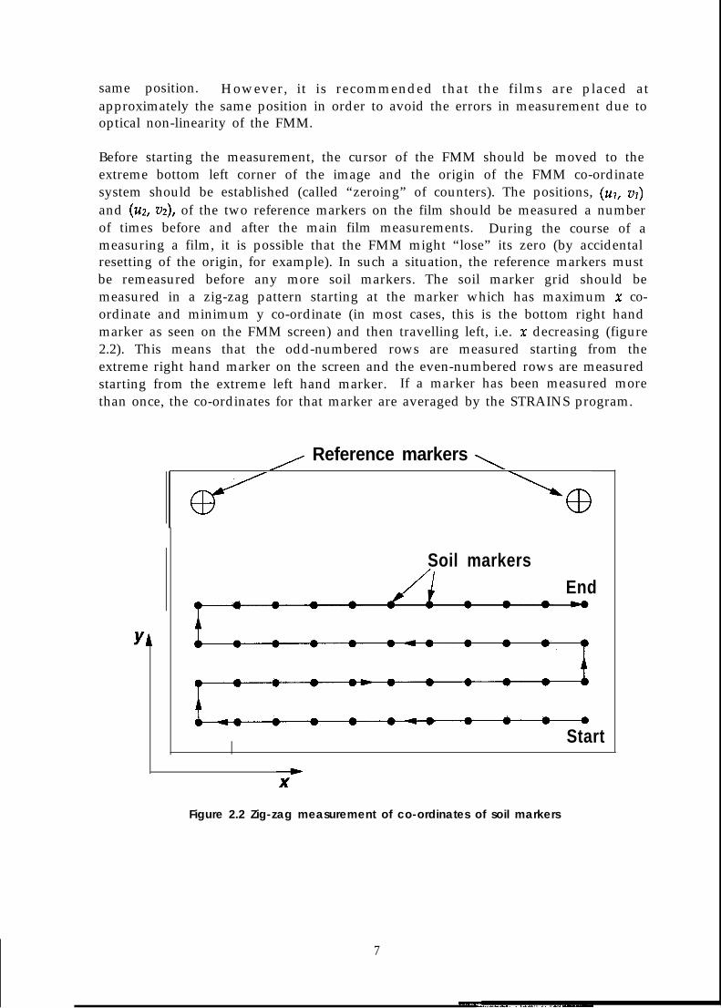
Before starting the measurement, the cursor of the FMM should be moved to theextreme bottom left corner of the image and the origin of the FMM co-ordinatesystem should be established (called “zeroing” of counters). The positions, (~1, ~1)and (2.42, ~4, of the two reference markers on the film should be measured a numberof times before and after the main film measurements. During the course of ameasuring a film, it is possible that the FMM might “lose” its zero (by accidentalresetting of the origin, for example). In such a situation, the reference markers mustbe remeasured before any more soil markers. The soil marker grid should bemeasured in a zig-zag pattern starting at the marker which has maximum x co-ordinate and minimum y co-ordinate (in most cases, this is the bottom right handmarker as seen on the FMM screen) and then travelling left, i.e. x decreasing (figure2.2). This means that the odd-numbered rows are measured starting from theextreme right hand marker on the screen and the even-numbered rows are measuredstarting from the extreme left hand marker. If a marker has been measured morethan once, the co-ordinates for that marker are averaged by the STRAINS program.

A Reference markers ,,

bl3

Soil markers

End

YA

Start

Figure 2.2 Zig-zag measurement of co-ordinates of soil markers

7

3. The STRAINS Program

3.1 An Overview

The STRAINS program is written to run on IBM PC and compatibles based on theINTEL 486 or higher processor. It supersedes the mainframe version of theSTRAINS program. It is written in FORTRAN-77 and has been compiled and linkedusing the Salford University FTN77 compiler. It uses the INTERACTER graphicslibrary for generating the plots. Since all the executable files created using theSalford University FTN77 compiler require a run-time system called DBOS for theirexecution, it must be present on the PC for running the STRAINS program.

3.2 Hardware and Software Requirements

STRAINS can be run on IBM PC and compatibles based on the INTEL 486 or higherprocessor. In addition, the computer should also satisfy the following requirements:

1. At least 4 Mb of RAM. 8 Mb preferred.2. At least 20 Mb of hard disk space.3. Maths co-processor4. At least a VGA colour monitor (640 x 480 pixels). SVGA preferred.5. MS-DOS 6.2 or higher.6. DBOS run-time system (Version 2.73 or higher).

3.3 Installation of STRAINS

STRAINS is supplied on a 3.5” double-sided high-density (1.44 Mb) floppy disk. Itneeds to be installed on to the hard disk of the computer. It can not be run from thefloppy disk. The following procedure should be followed for its correct installationon the hard disk:

1. Switch on the computer and wait for the DOS prompt

C:\>

2. Insert the floppy disk containing the STRAINS program into the floppydrive (assumed to be drive A).

3. Switch to the floppy drive (assumed to be drive A) as follows:

C:\>A: J

4. At the prompt, type INSTALL and press RETURN (.J) as follows:

A:\>INSTALL .-I

5. The installation program should now begin to copy the files from thefloppy on to the hard disk in a directory called STRAINS. Wait for theinstallation to be complete. After the completion of the installation, thefollowing message should be displayed on your computer:

STRAINS program successfully installed !!

and the computer should return the following prompt:

C:\STRAINS>

The STRAINS program is now ready for execution.

3.4 Running the STRAINS program

3.4.1 File Handling Strategy

The STRAINS program needs an analysis identifier before any of its modules can beexecuted. The analysis identifier should be less than or equal to 8 characters inlength. It should be a valid DOS file name. For instance, the user may find itconvenient give the centrifuge test code as the analysis identifier. All the files thatare either used or created by the STRAINS program have the analysis identifier astheir name. These files are distinguished from one another by different extensions.For example, the parametric file for an analysis called BOND007 is named asBOND007PAR whereas the results file for the same analysis is named asBOND007RES. The analysis identifier can be set using the DOS parameter STRFLN(acronym for STRains File Name). The user should type the following after theprompt to set the analysis identifier:

SET STRFLN = <analysis identifier> J

For example, in order to set BOND007 as the analysis identifier, one should type:

SET STRFLN = BOND007 J

The STRAINS program can now be started by typing STRAINS after the prompt andpressing RETURN. If STRFLN is not set, the execution of STRAINS will terminateafter displaying the following message:

9

The DOS Parameter STRFLN is not set. In order touse the STRAINS program, STRFLN must be set to thetest identifier. Quit the STRAINS main menu, returnto the DOS prompt and set STRFLN.

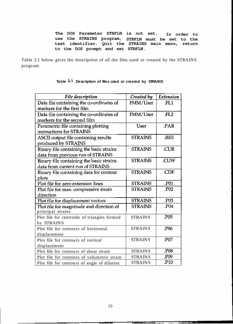
Table 3.1 below gives the description of all the files used or created by the STRAINSprogram.

Table 3.1 Description of files used or created by STRAINS

principal strainsPlot file for centroids of triangles formedby STRAINS

STRAINS PO5

Plot file for contours of horizontaldisplacement

STRAINS .I?06

Plot file for contours of verticaldisplacementPlot file for contours of shear strainPlot file for contours of volumetric strainPlot file for contours of angle of dilation

STRAINS PO7

STRAINS PO8STRAINS PO9STRAINS HO

10

3.4.2 Various Menus in STRAINS

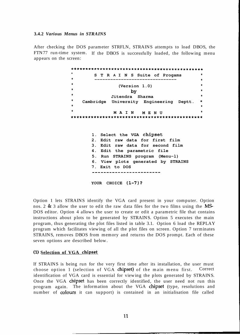
After checking the DOS parameter STRFLN, STRAINS attempts to load DBOS, theFTN77 run-time system. If the DBOS is successfully loaded, the following menuappears on the screen:

*********************************************** S T R A I N S Suite of Progams ** ------------------------------- ** (Version 1.0) ** by ** Jitendra Sharma ** Cambridge University Engineering Deptt. ** ** M A I N M E N U ***********************************************

1. Select the VGA chipset2. Edit raw data for first film3. Edit raw data for second film4. Edit the parametric file5. Run STRAINS program (Menu-l)6. View plots generated by STRAINS7. Exit to DOS

YOUR CHOICE (l-7)?

Option 1 lets STRAINS identify the VGA card present in your computer. Optionnos. 2 & 3 allow the user to edit the raw data files for the two films using the MS-DOS editor. Option 4 allows the user to create or edit a parametric file that containsinstructions about plots to be generated by STRAINS. Option 5 executes the mainprogram, thus generating the plot files listed in table 3.1. Option 6 load the REPLAYprogram which facilitates viewing of all the plot files on screen. Option 7 terminatesSTRAINS, removes DBOS from memory and returns the DOS prompt. Each of theseseven options are described below.

(1) Selection of VGA chipset

If STRAINS is being run for the very first time after its installation, the user mustchoose option 1 (selection of VGA chipset) of the main menu first. Correctidentification of VGA card is essential for viewing the plots generated by STRAINS.Once the VGA chipset has been correctly identified, the user need not run thisprogram again. The information about the VGA chipset (type, resolutions andnumber of colours it can support) is contained in an initialisation file called

STRAINS.INI. STRAINS reads this information prior to displaying its banners andplot files. At present, STRAINS can identify the following VGA chipsets:

Tseng Labs ET3000, Tseng Labs ET4000, Paradise, Video 7, Everex, ATI,Trident, Chips & Technologies 82c452/82c453, Ahead B, Oak Technology,Genoa GVGA, NCR 77C20/21/22E, S3 86C911/924, Cirrus 5442,Primus 2000, Olivetti, Toshiba, Realtek, Vesa.

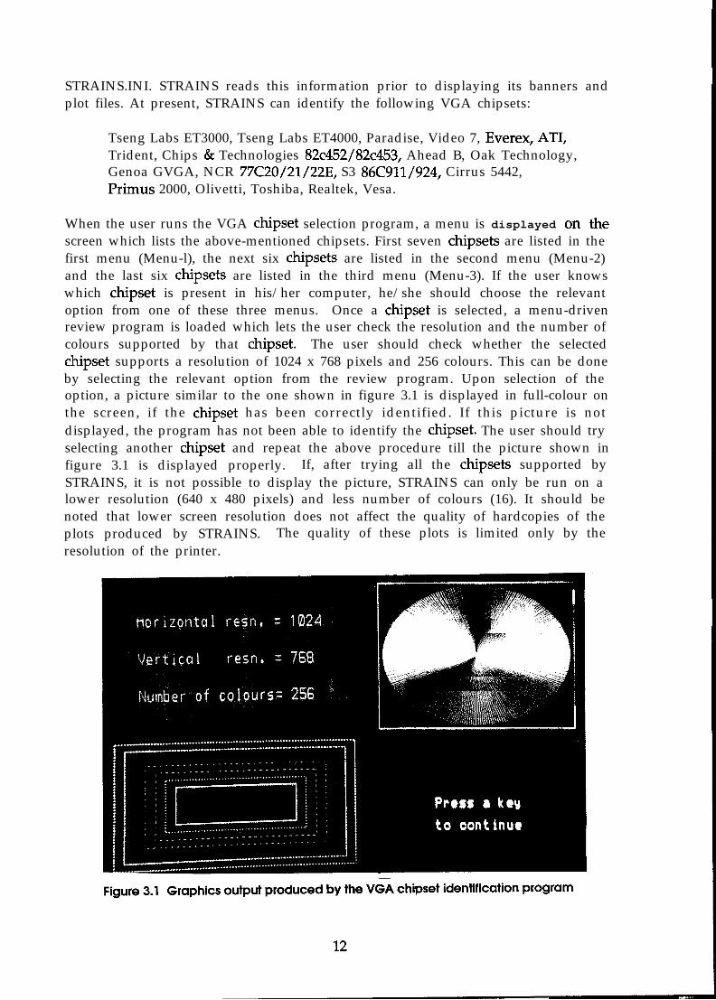
When the user runs the VGA chipset selection program, a menu is displayed on thescreen which lists the above-mentioned chipsets. First seven chipsets are listed in thefirst menu (Menu-l), the next six chipsets are listed in the second menu (Menu-2)and the last six chipsets are listed in the third menu (Menu-3). If the user knowswhich chipset is present in his/her computer, he/she should choose the relevantoption from one of these three menus. Once a chipset is selected, a menu-drivenreview program is loaded which lets the user check the resolution and the number ofcolours supported by that chipset. The user should check whether the selectedchipset supports a resolution of 1024 x 768 pixels and 256 colours. This can be doneby selecting the relevant option from the review program. Upon selection of theoption, a picture similar to the one shown in figure 3.1 is displayed in full-colour onthe screen, if the chipset has been correctly identified. If this picture is notdisplayed, the program has not been able to identify the chipset. The user should tryselecting another chipset and repeat the above procedure till the picture shown infigure 3.1 is displayed properly. If, after trying all the chipsets supported bySTRAINS, it is not possible to display the picture, STRAINS can only be run on alower resolution (640 x 480 pixels) and less number of colours (16). It should benoted that lower screen resolution does not affect the quality of hardcopies of theplots produced by STRAINS. The quality of these plots is limited only by theresolution of the printer.

(2) & (3) Edit’lng raw data for the two films

As mentioned above, choosing option 2 (or option 3) loads the raw data file for firstfilm (or second film) into the MS-DOS editor. All the steps required when editingthe raw data file are given below:

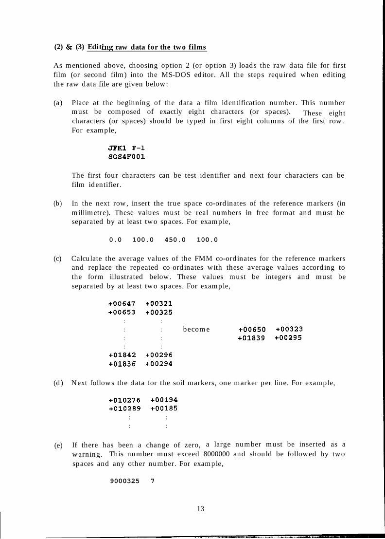
(a) Place at the beginning of the data a film identification number. This numbermust be composed of exactly eight characters (or spaces). These eightcharacters (or spaces) should be typed in first eight columns of the first row.For example,

JFKl F-lSOS4F001

The first four characters can be test identifier and next four characters can befilm identifier.

(b) In the next row, insert the true space co-ordinates of the reference markers (inmillimetre). These values must be real numbers in free format and must beseparated by at least two spaces. For example,

0.0 100.0 450.0 100.0

(c) Calculate the average values of the FMM co-ordinates for the reference markersand replace the repeated co-ordinates with these average values according tothe form illustrated below. These values must be integers and must beseparated by at least two spaces. For example,

+00647 +00321+00653 +00325

: :: : become +00650 +00323: : +01839 +00295: :

+01842 +00296+01836 +00294

(d) Next follows the data for the soil markers, one marker per line. For example,

+010276 +00194+010289 +00185

: :: :

(e) If there has been a change of zero, a large number must be inserted as awarning. This number must exceed 8000000 and should be followed by twospaces and any other number. For example,

9000325 7

13

(f) Following this warning, a new set of real space reference marker co-ordinatesand average FMM reference marker co-ordinates must be inserted as shown insteps (b) and (c).

(g) The new FMM reference marker co-ordinates are followed by the soil markerco-ordinates as in step (d).

(h) The FMM data are terminated by a negative number. For example,

-1 0

This should be the last line in the input data.

(4) Editing the parametric file

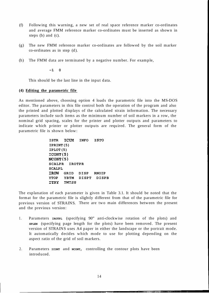
As mentioned above, choosing option 4 loads the parametric file into the MS-DOSeditor. The parameters in this file control both the operation of the program and alsothe printed and plotted displays of the calculated strain information. The necessaryparameters include such items as the minimum number of soil markers in a row, thenominal grid spacing, scales for the printer and plotter outputs and parameters toindicate which printer or plotter outputs are required. The general form of theparametric file is shown below:

ISTR ICUM INFO ISTOIPRINT(5)IPLOT(5)ICONT(5)NCONT(5)SCALPR IROTPRSCALPLIROW GRID DISP RNOIPYTOP YBTM DISPT DISPBITRY IMISS

The explanation of each parameter is given in Table 3.1. It should be noted that theformat for the parametric file is slightly different from that of the parametric file forprevious version of STRAINS. There are two main differences between the presentand the previous version:

1 . Parameters IROTPL (specifying 90” anti-clockwise rotation of the plots) andSPLEN (specifying page length for the plots) have been removed. The presentversion of STRAINS uses A4 paper in either the landscape or the portrait mode.It automatically decides which mode to use for plotting depending on theaspect ratio of the grid of soil markers.

14

2. Parameters ICONT and NCONT, controlling the contour plots have beenintroduced.

Therefore, the users of previous version of STRAINS upgrading to the presentversion, need to modify the existing parametric files to take into account the abovechanges.

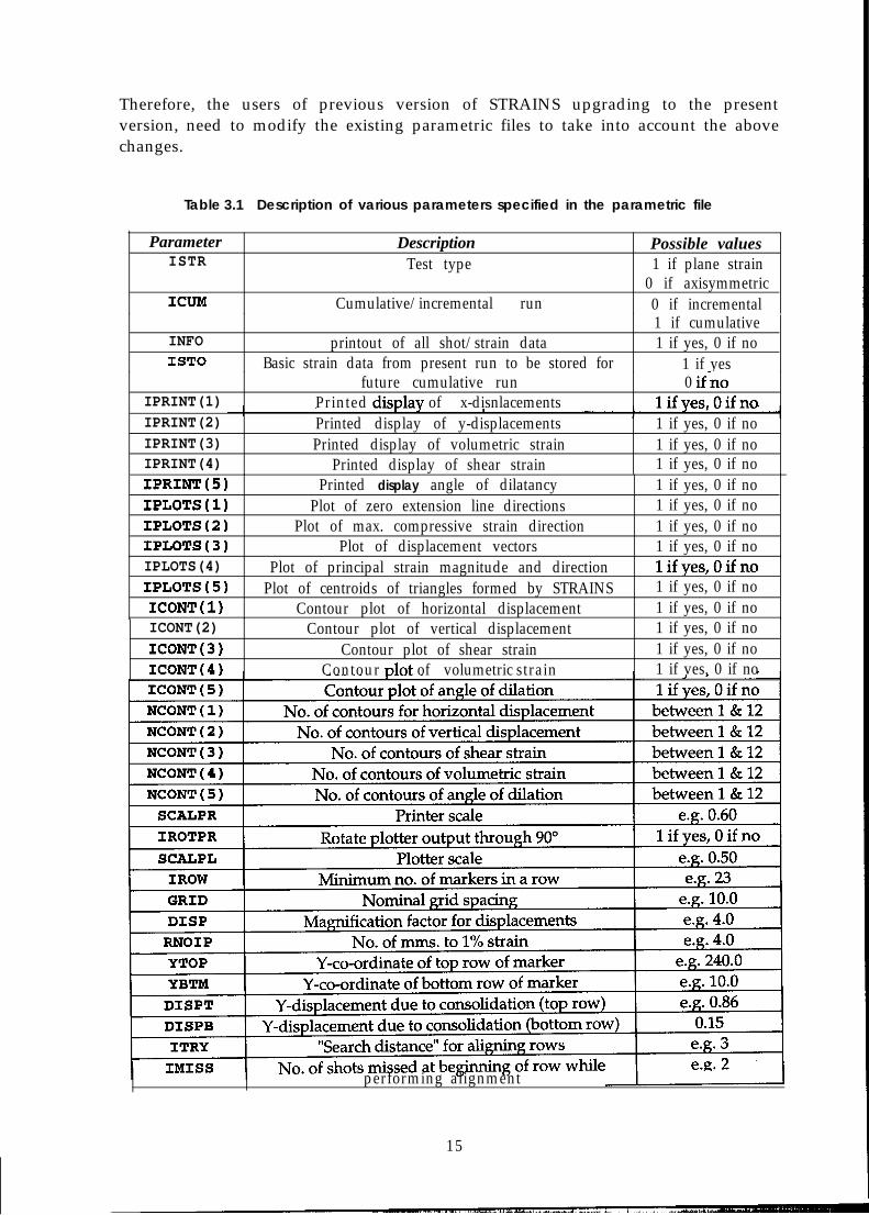
Table 3.1 Description of various parameters specified in the parametric file

ParameterISTR

ICUM

DescriptionTest type

Cumulative/incremental run

Possible values1 if plane strain

0 if axisymmetric0 if incremental

INFOISTO

printout of all shot/strain dataBasic strain data from present run to be stored for

1 if cumulative1 if yes, 0 if no

1 if yes

IPRINT(1)future cumulative run

Printed disnlav of x-disnlacements0 ifno

lifves.OifnoIPRINT(2)

IPRINT(5)

IPRINT(3)

IPLOTS(1)

IPRINT(4)

IPLOTS(2)IPLOTS(3)IPLOTS(4)

ICONT(2)

IPLOTS(5)

ICONT(3)

ICONT(1)

ICONT(4)

Plot of principal strain magnitude and direction

Printed display of y-displacements

Printed display angle of dilatancy

Plot of centroids of triangles formed by STRAINS

Plot of zero extension line directions

Printed display of volumetric strain

Plot of max. compressive strain direction

Contour plot of horizontal displacement

Printed display of shear strain

Plot of displacement vectors

1 if yes, 0 if no

1 if yes, 0 if no

1 if yes, 0 if no

1 if yes, 0 if no

1 if yes, 0 if no

1 if yes, 0 if no1 if yes, 0 if nolifyes,Oifno

1 if yes, 0 if no

1 if yes, 0 if no

1 if yes, 0 if no

1 if yes, 0 if no

1 if ves, 0 if no

Contour plot of vertical displacementContour plot of shear strain

Contour nlot of volumetric strain

performing alignment

15

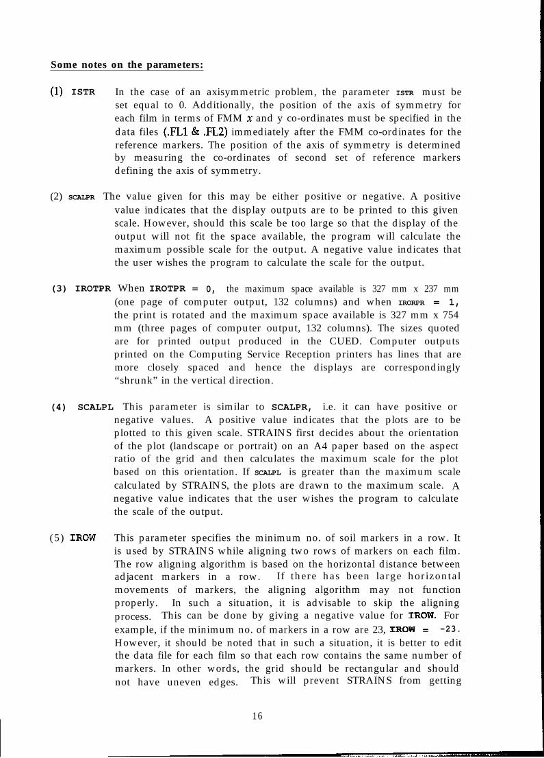
Some notes on the parameters:

(1) ISTR In the case of an axisymmetric problem, the parameter ISTR must beset equal to 0. Additionally, the position of the axis of symmetry foreach film in terms of FMM x and y co-ordinates must be specified in thedata files (.FLl & .FL2) immediately after the FMM co-ordinates for thereference markers. The position of the axis of symmetry is determinedby measuring the co-ordinates of second set of reference markersdefining the axis of symmetry.

(2) SCALPR The value given for this may be either positive or negative. A positivevalue indicates that the display outputs are to be printed to this givenscale. However, should this scale be too large so that the display of theoutput will not fit the space available, the program will calculate themaximum possible scale for the output. A negative value indicates thatthe user wishes the program to calculate the scale for the output.

(3) IROTPR When IROTPR = 0, the maximum space available is 327 mm x 237 mm(one page of computer output, 132 columns) and when IRORPR = 1,the print is rotated and the maximum space available is 327 mm x 754mm (three pages of computer output, 132 columns). The sizes quotedare for printed output produced in the CUED. Computer outputsprinted on the Computing Service Reception printers has lines that aremore closely spaced and hence the displays are correspondingly“shrunk” in the vertical direction.

(4) SCALPL This parameter is similar to SCALPR, i.e. it can have positive ornegative values. A positive value indicates that the plots are to beplotted to this given scale. STRAINS first decides about the orientationof the plot (landscape or portrait) on an A4 paper based on the aspectratio of the grid and then calculates the maximum scale for the plotbased on this orientation. If SCALPL is greater than the maximum scalecalculated by STRAINS, the plots are drawn to the maximum scale. Anegative value indicates that the user wishes the program to calculatethe scale of the output.

(5) IROW This parameter specifies the minimum no. of soil markers in a row. Itis used by STRAINS while aligning two rows of markers on each film.The row aligning algorithm is based on the horizontal distance betweenadjacent markers in a row. If there has been large horizontalmovements of markers, the aligning algorithm may not functionproperly. In such a situation, it is advisable to skip the aligningprocess. This can be done by giving a negative value for IROW. Forexample, if the minimum no. of markers in a row are 23, IROW = -23.However, it should be noted that in such a situation, it is better to editthe data file for each film so that each row contains the same number ofmarkers. In other words, the grid should be rectangular and shouldnot have uneven edges. This will prevent STRAINS from getting

16

confused when it forms triangles with soil markers from two adjacentrows on a film.

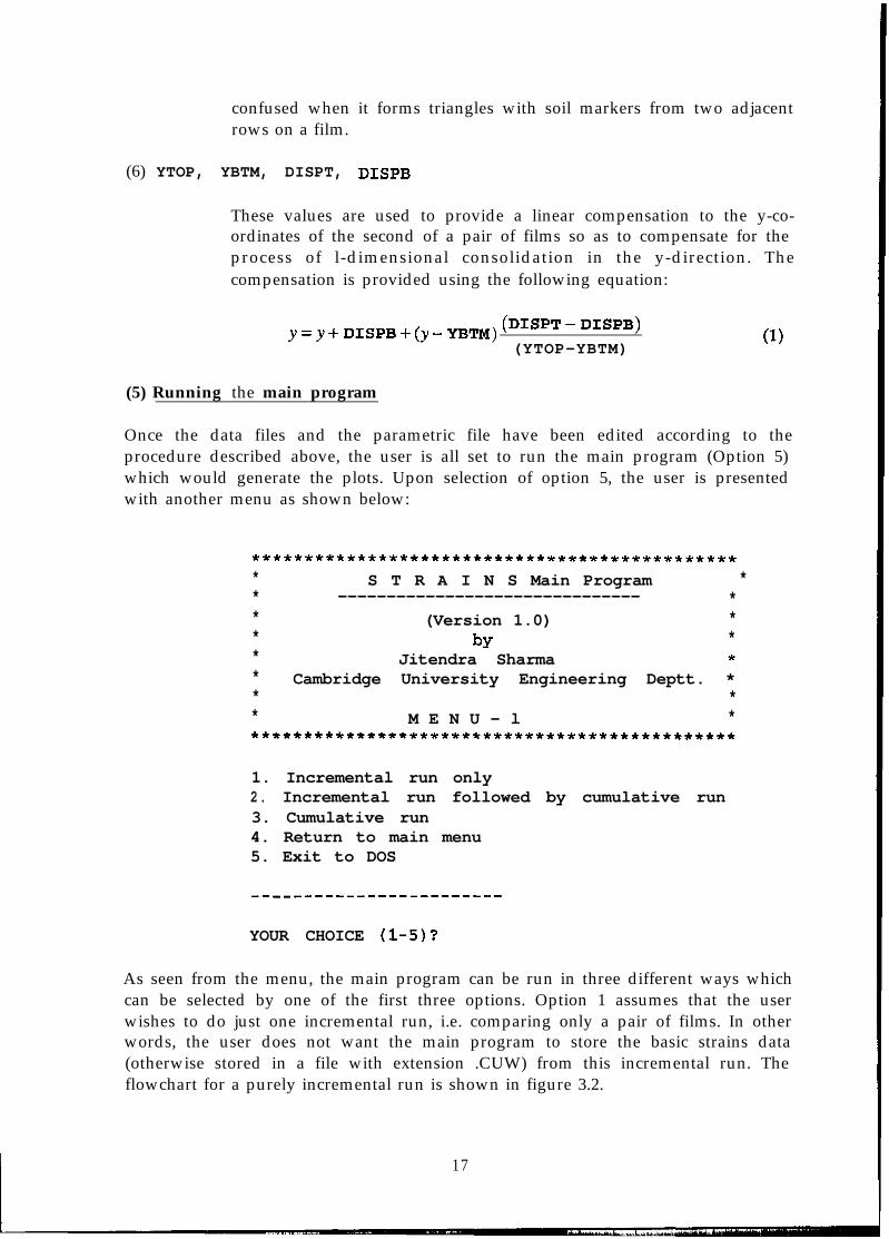
(6) YTOP, YBTM, DISPT, DISPB

These values are used to provide a linear compensation to the y-co-ordinates of the second of a pair of films so as to compensate for theprocess of l-dimensional consolidation in the y-direction. Thecompensation is provided using the following equation:

y=y+DISPB+(y-YBTM)(DISPT-DI~PB)

(YTOP-YBTM) (1)

(5) Running the main program

Once the data files and the parametric file have been edited according to theprocedure described above, the user is all set to run the main program (Option 5)which would generate the plots. Upon selection of option 5, the user is presentedwith another menu as shown below:

*********************************************** S T R A I N S Main Program ** ------------------------------- ** (Version 1.0) ** by ** Jitendra Sharma ** Cambridge University Engineering Deptt. ** ** M E N U - l ***********************************************

1. Incremental run only2. Incremental run followed by cumulative run3. Cumulative run4. Return to main menu5. Exit to DOS

YOUR CHOICE (l-5)?

As seen from the menu, the main program can be run in three different ways whichcan be selected by one of the first three options. Option 1 assumes that the userwishes to do just one incremental run, i.e. comparing only a pair of films. In otherwords, the user does not want the main program to store the basic strains data(otherwise stored in a file with extension .CUW) from this incremental run. Theflowchart for a purely incremental run is shown in figure 3.2.

17

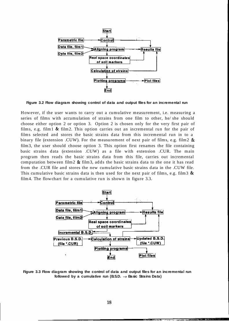
Figure 3.2 Flow diagram showing control of data and output files for an incremental run

However, if the user wants to carry out a cumulative measurement, i.e. measuring aseries of films with accumulation of strains from one film to other, he/she shouldchoose either option 2 or option 3. Option 2 is chosen only for the very first pair offilms, e.g. film1 & film2. This option carries out an incremental run for the pair offilms selected and stores the basic strains data from this incremental run in to abinary file (extension .CUW). For the measurement of next pair of films, e.g. film2 &film3, the user should choose option 3. This option first renames the file containingbasic strains data (extension .CUW) as a file with extension .CUR. The mainprogram then reads the basic strains data from this file, carries out incrementalcomputation between film2 & film3, adds the basic strains data to the one it has readfrom the .CUR file and stores the new cumulative basic strains data in the .CUW file.This cumulative basic strains data is then used for the next pair of films, e.g. film3 &film4. The flowchart for a cumulative run is shown in figure 3.3.

Figure 3.3 Flow diagram showing the control of data and output files for an incremental runfollowed by a cumulative run (B.S.D. + Basic Strains Data)

After the relevant option has been selected, the main program displays its banner.The execution commences as soon as the user presses the RETURN key (+I). Themain program then displays a banner asking user to wait while it generates theoutput (results and plots). The following message is displayed at the end ofexecution:

****** STRAINS RUN FINISHED.

The following file(s) have been created:

Printed Output (Results) :---- <analysis id.>.RES

Press any key to continue......

Pressing any key displays the main menu. The user can now view the plotsgenerated by STRAINS on the VDU screen.

(6) Viewing plots on the VDU screen

If the user wishes to look at the plots generated by STRAINS, he/she can do it bychoosing option 6. Selecting option 6 loads the REPLAY program. The REPLAYprogram lets the user view the plots on VDU screen. This program is also menu-driven. REPLAY recognises the plots using their extensions (*PO1 to *.PlO). SinceREPLAY can also display the plots generated from another analysis, the user isasked to enter the analysis identifier. By default, REPLAY will display plotsgenerated by the analysis specified by the DOS parameter STRFLN. REPLAY can beterminated by typing S. After terminating REPLAY, the main menu is displayedonce again.

(7) Exit to DOS

The STRAINS program can be terminated by choosing option 7 from the main menu.Upon selection of this option, the DBOS run-time system is removed from thememory. A message to this effect is displayed before the DOS prompt is returned.The user is advised to make sure this message is displayed before running any otherprogram such as MS-Windows because if the DBOS is not removed from thememory, other programs won’t work. Forced removal of DBOS can be done bytyping the following after the DOS prompt:

KILL-DBOS J

19

Appendix A: The Calculation of Strains

A.1 Introduction

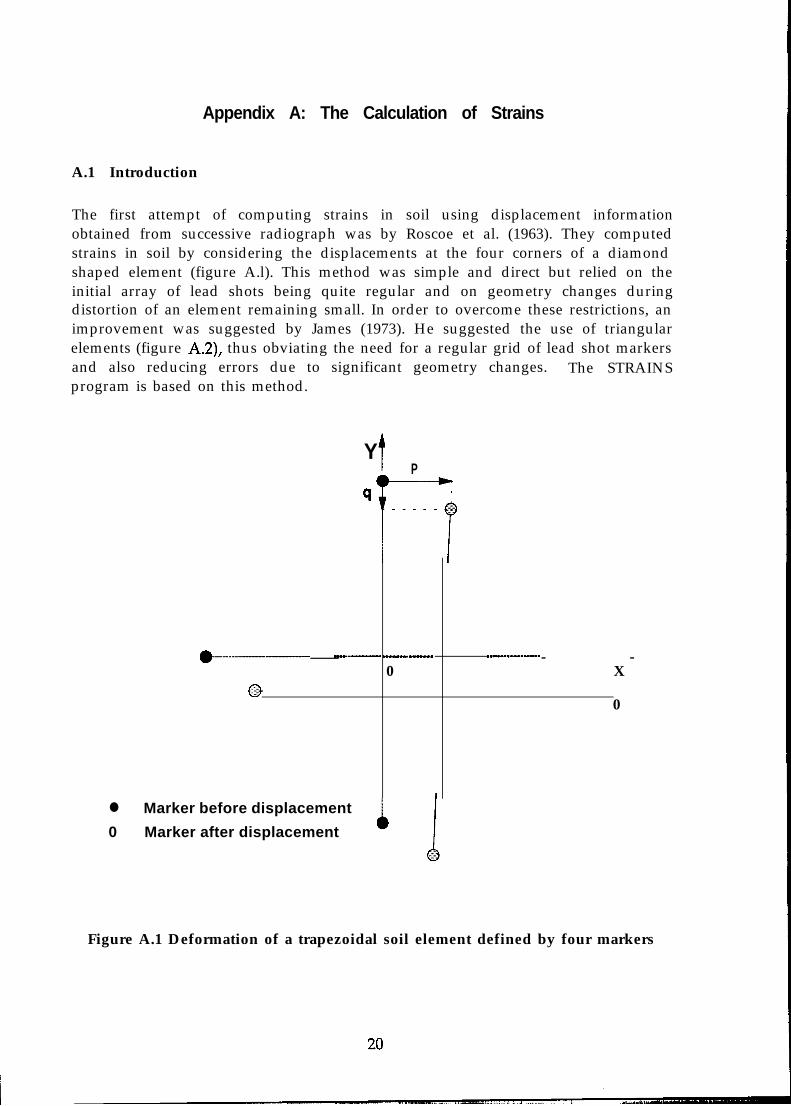
The first attempt of computing strains in soil using displacement informationobtained from successive radiograph was by Roscoe et al. (1963). They computedstrains in soil by considering the displacements at the four corners of a diamondshaped element (figure A.l). This method was simple and direct but relied on theinitial array of lead shots being quite regular and on geometry changes duringdistortion of an element remaining small. In order to overcome these restrictions, animprovement was suggested by James (1973). He suggested the use of triangularelements (figure A.2), thus obviating the need for a regular grid of lead shot markersand also reducing errors due to significant geometry changes. The STRAINSprogram is based on this method.

Yt P

q

*-----_______ - __-_- - ___- --___ _---_--------- -0 X

0

l Marker before displacement

0 Marker after displacement A

Figure A.1 Deformation of a trapezoidal soil element defined by four markers

A Reference markers ,,

Triangular elements Soil markers

0 0 A 0 0 0 l

0 0 0 l 0 0 l 0

0 0 l 0 0 l l 0 0 l l

0 0 l 0 0 l l 0 l l l

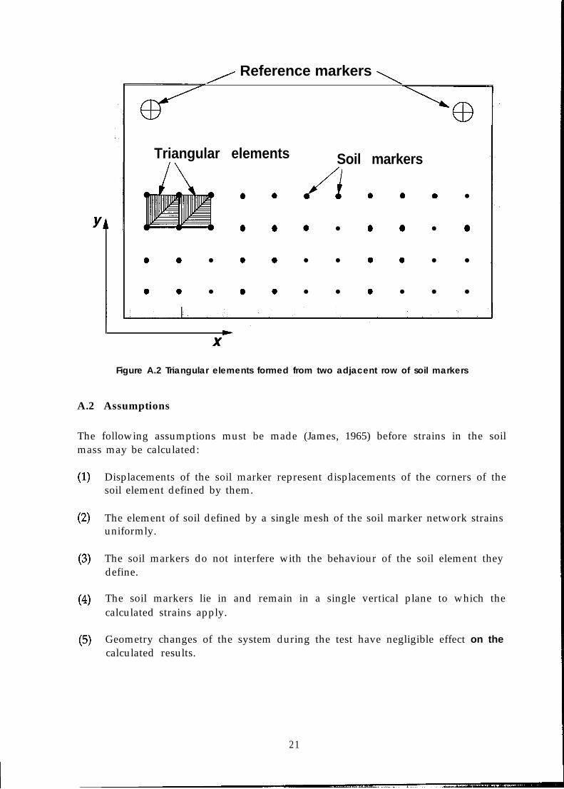
Figure A.2 Triangular elements formed from two adjacent row of soil markers

A.2 Assumptions

The following assumptions must be made (James, 1965) before strains in the soilmass may be calculated:

(1)

(2)

(3)

(4)

(5)

Displacements of the soil marker represent displacements of the corners of thesoil element defined by them.

The element of soil defined by a single mesh of the soil marker network strainsuniformly.

The soil markers do not interfere with the behaviour of the soil element theydefine.

The soil markers lie in and remain in a single vertical plane to which thecalculated strains apply.

Geometry changes of the system during the test have negligible effect on thecalculated results.

21

A.3 The Transformation of Co-ordinates

The built-in co-ordinate system of the FMM is a normal right-handed Cartesiansystem with all distances measured in microns. However, since no two films can beplaced in exactly the same position on the FMM, it is necessary to relate the FMM co-ordinate for each marker to the same co-ordinate system. The new co-ordinatesystem is related to the geometry of the apparatus (e.g. strongbox). Let us call thisnew co-ordinate system the real space svstem. The co-ordinates in the real spacesystems are expressed in millimetre. Since the co-ordinates of the reference markersare known both in the FMM space and in the real space system, it is possible tocompute the transformation matrix between the two systems.

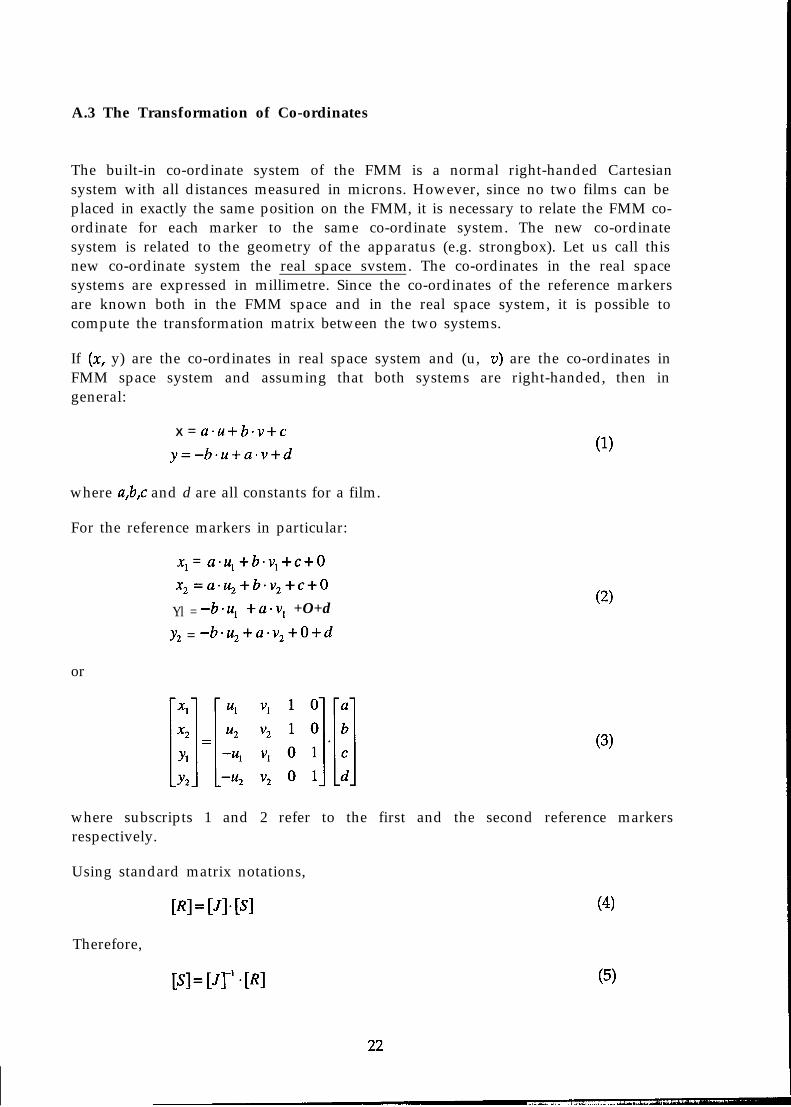
If (x, y) are the co-ordinates in real space system and (u, V) are the co-ordinates inFMM space system and assuming that both systems are right-handed, then ingeneral:

X = a-u+ b.v+c

y=-b.u+a.v+d (1)

where a,b,c and d are all constants for a film.

For the reference markers in particular:

x, = a.u, +b.v, +c+O

x2 =aeu,+b.v,+c+O

Yl = -b.u, +aav, +O+d

Yz = -b.u, +a.v,+O+d

or

(2)

(3)

where subscripts 1 and 2 refer to the first and the second reference markersrespectively.

Using standard matrix notations,

Therefore,

(4)

(5)

Hence, the constants a,b,c and d can be found from the co-ordinates of the referencemarkers. It is now possible to use equation (1) to transform the co-ordinates of allthe markers in the grid into the real space system. Consequently, the displacementsof the markers between successive films can be calculated and strain information canbe derived from these displacements.

A.4 Calculation of displacements and strains

The grid of soil markers is divided into a series of triangular elements (figure A.2).These triangular elements are used as a basis for strain computations. A typicaltriangular element is shown in figure A.3 where, for convenience, the origin of co-ordinates is taken at the corner i.

Figure A.3 Initial and displaced positions of a triangular element

The assumed uniform strain is taken to be caused by a linear displacement field.Thus, the displacements p and LJ are given by

p=p,+A-x+Bq

q=qi+c*x+ll*y(6)

where A,B,C and D are all constants and can be determined from the measureddisplacements of the corners.

23

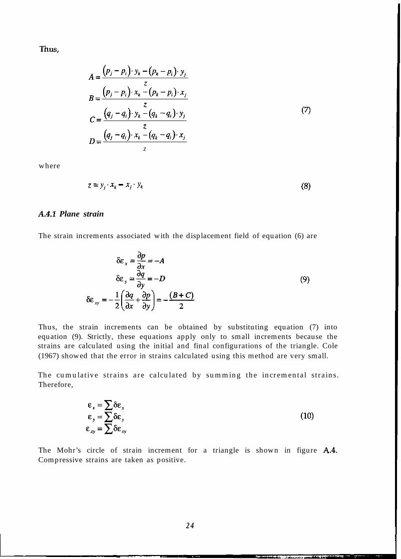
ThUS,

A= (Pj-Pi)‘Yk-(Pk-Pi)‘Yj

B= (PjsPi)‘xk ‘(Pk-Pi)‘xj

c= (4j -4i).Yk ‘(4k -4i)‘Yj

D= (4j -e)*xk ‘(qk -4i)‘xj

z

where

Z = Yj ’ Xk - xj ’ Yk (8)

A.4.1 Plane strain

The strain increments associated with the displacement field of equation (6) are

Thus, the strain increments can be obtained by substituting equation (7) intoequation (9). Strictly, these equations apply only to small increments because thestrains are calculated using the initial and final configurations of the triangle. Cole(1967) showed that the error in strains calculated using this method are very small.

The cumulative strains are calculated by summing the incremental strains.Therefore,

(10)

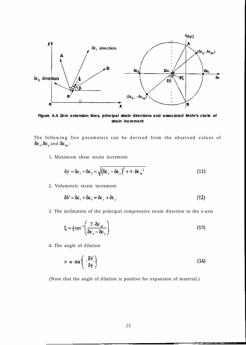
The Mohr’s circle of strain increment for a triangle is shown in figure A.4.Compressive strains are taken as positive.

2 4

&, direction

B

&, direction

jj-

5

a1

XX

Figure A.4 Zero extension lines, principal strain directions and associated Mohr’s circle ofstrain increment

Figure A.4 Zero extension lines, principal strain directions and associated Mohr’s circle ofstrain increment

The following five parameters can be derived from the observed values ofSQk, and SE, :

1. Maximum shear strain increment

2. Volumetric strain increment

SV=S&, +s&, =SE, +s&, (12)

3. The inclination of the principal compressive strain direction to the x-axis

4. The angle of dilation

6Vv = sin-’ - -c 1SY(14)

(Note that the angle of dilation is positive for expansion of material.)

25

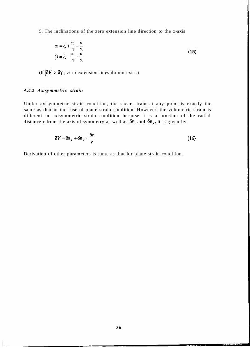
5. The inclinations of the zero extension line direction to the x-axis

(If lSVl> 6~ , zero extension lines do not exist.)

A.4.2 Axisymmetric strain

Under axisymmetric strain condition, the shear strain at any point is exactly thesame as that in the case of plane strain condition. However, the volumetric strain isdifferent in axisymmetric strain condition because it is a function of the radialdistance r from the axis of symmetry as well as SE, and SE,. It is given by

(16)

Derivation of other parameters is same as that for plane strain condition.

2 6

Appendix B: Editing the plot files using Lotus Freelance

B.l Introduction

Although every effort has been made to generate plots which are self-explanatory,the user may wish to modify them to achieve better presentation of results. Forexample, the user may find it useful to draw the outline of the package around thegrid of soil markers or to add few more captions. This can be achieved by importingthe plot files into any graphics editor which has a filter for HP-GL files. One suchgraphics editor is the Lotus Freelance for Windows (ver. 2.01). This section of themanual briefly describes the procedure for editing the plot files using the LotusFreelance for Windows.

B.2 Importing the plot file into Lotus Freelance

Before importing the plot files into Lotus Freelance, the user is strongly advised tocritically examine the validity of results produced by STRAINS by previewing themon screen using the REPLAY program. Once the user is satisfied about thecorrectness of the results, he/she is ready to edit the plot files.

The graphics filter for importing HP-GL plot files is usually supplied with LotusFreelance for Windows. However, it is a good idea to check whether the versionbeing used has this filter. Start MS-Windows as usual and start the Lotus Freelanceby double-clicking on its icon. Choose “blank” smartmaster background and choose“none” as the basic layout. This should display a white blank page. From the FILEmenu, choose IMPORT. Another window should appear on top of the mainwindow. Inside this window, there is a sub-window titled “File Type”. Scroll insidethis sub-window and look for “Hewlett-Packard Graphics Language (HGL)“. If theuser finds this inside the sub-window, the version of Lotus Freelance being used hasa graphics filter for HP-GL plot files.

A peculiar thing about the HP-GL graphics filter available in Lotus Freelance is thatit can recognise the HP-GL plot file solely on the basis of its extension. It expects theextension for such a file to be .HGL. However, the plot files generated by STRAINShave extensions PO1 to .PlO. This means that the user has to either copy the plot filewhich he/she wants to edit to a new file having an extension .HGL or he/she mayprefer to rename that plot file and specify a .HGL extension for it. Once this is done,the plot file can be imported by choosing IMPORT from the FILE menu as describedabove. The user may have to tell the location of the plot file (directory) to LotusFreelance. After the completion of IMPORT, the plot file should appear in the mainwindow.

2 7

B.3 Editing the imported plot file

The imported plot file is stored in vector format by Lotus Freelance, i.e. it containsnothing else but lines either joined or free. Even the alphabetical characters andnumerals are stored as joined lines. By default, all the lines present in the importedplot files are grouped together by Lotus Freelance. In order to edit this file, it shouldbe ungrouped. This can be done by choosing UNGROUP from the ARRANGEmenu. Once the plot file is ungrouped, each line becomes an object and itsproperties can be manipulated using the tools available in Lotus Freelance. The usercan now do whatever he/she wishes (within the capabilities of Lotus Freelance, ofcourse !) to this file. For example, the outer frame of the plot can be deleted andreplaced by a line diagram representing boundary of the package. New captions canbe added. Colour, thickness or style of some of the lines may be changed.

Once the editing is complete, the user may save this file as Lotus Freelancepresentation file (extension PRE). Alternatively, he/she can store the plot as either ametafile or an encapsulated postscript file. This can be done by choosing EXPORTfrom the FILE menu and clicking on the relevant format. Once the edited file hasbeen exported in any one of the many formats available in Lotus Freelance, it caneasily be incorporated in any document using a sophisticated word processingsoftware such as MS-Word for Windows or WordPerfect for Windows.

2 8

References

Britto, A.M. (1984). A User’s Guide to the Soils Strain Calculating Program. InternalReport, Cambridge University Engineering Department.

Cole, E.R.L. (1967). Soils in simple shear apparatus. Ph.D. thesis. CambridgeUniversity.

James, R.G. (1965). Stress and strain fields in sand. Ph.D. thesis. CambridgeUniversity.

James, R.G. (1973). Determination of strains in soil by radiography. TechnicalReport CUED/C-Soils/LNl(a). Cambridge University EngineeringDepartment.

Phillips, R. (1991). Film Measurement Machine: User Munuul. Technical ReportCUED/D-Soils/TR246. Cambridge University Engineering Department.

Roscoe, K.H., Arthur, J.R.F. and James, R.G. (1963). The determination of strains insoil by an X-ray method. Civil Engineering and Public Works Review, Vol. 58,No. 684, pp 873-876 (Part 1) & No. 685, pp 1009-1012 (Part 2).

Schofield, A.N. (1980). Cambridge geotechnical centrifuge operations. Gkotechnique,Vol. 30, No. 3, pp 227-268.

29