Embed Size (px)
Citation preview
December 12, 2013 21:24 WSPC/130-JCA AP1˙after˙revision
Journal of Computational Acousticsc© IMACS
A two-dimensional study of finite amplitude sound waves in a trumpet using
the discontinuous Galerkin method
JANELLE RESCH∗
Applied Mathematics, University of Waterloo,[email protected]
LILIA KRIVODONOVA
Applied Mathematics, University of Waterloo,Waterloo, ON, Canada N2L 3G1
JOHN VANDERKOOY
Physics and Astronomy, University of Waterloo,Waterloo, Waterloo, ON, Canada N2L 3G1
A model for nonlinear sound wave propagation for the trumpet is proposed. Experiments havebeen carried out to measure the sound pressure waveforms of the Bb
3 and Bb4 notes played forte.
We use these pressure measurements at the mouthpiece as an input for the proposed model. Thecompressible Euler equations are used to incorporate nonlinear wave propagation and compress-ibility effects. The equations of motion are solved using the discontinuous Galerkin method (DGM)and the suitability of this method is assessed. The third spatial dimension is neglected and theconsequences for such an assumption are examined. The numerical experiments demonstrate thevalidity of this approach. We obtain a good match between experimental and numerical data afterthe dimensionality of the problem is taken into account.
Keywords: Nonlinear acoustic wave propagation; DGM; trumpet; sound pressure measurements;wave steepening; shock waves.
1. Introduction
The amplitude of most audible sound waves is only a small fraction of atmospheric pressure.
In such cases, a small amplitude linearization of the gas dynamics equations can be made
resulting in a linear model of sound propagation 1. However, for brass musical instruments
these simplifying assumptions start to break down once loud or high frequency notes are
played 1. For such notes, the pressure variations can be a significant fraction of atmospheric
pressure in the narrow tubing of the instrument 2. This can potentially allow the nonlinear
behavior from the high amplitude propagating waves to distort the waveforms 1,3.
If the pressure pulse leaving the mouthpiece of an instrument has large enough ampli-
tude, the crest will travel noticeably faster than the trough. This will cause the waveform
∗Waterloo, Waterloo, Ontario, Canada N2L 3G1
1
December 12, 2013 21:24 WSPC/130-JCA AP1˙after˙revision
2 J. Resch, L. Krivodonova & J. Vanderkooy
to steepen and excite the higher frequency components 4. This influences the timbre of the
sound giving it a more ‘brassy’ effect 5. If the cylindrical bore of the instrument is long
enough and the nonlinear effects are strong enough, it is possible for the wave to steepen
into a shock wave exaggerating the brassy sound 1.
Work addressing wave production for the trumpet began in 1971 by Bachus et al. 6, and
for the trombone in 1982 by Elliot et al. 7. In these papers, the motion of the lips coupled
to the air column was examined. They concluded that the nonlinear motion of the lips did
not contribute to the harmonic generation. They also thought that the amplitude of the
sound waves did not influence the wave propagation behavior. Bachus et al. 6 state that the
transfer function between the mouthpiece pressure and radiated sound was basically linear.
Since they assumed that the wave propagation could be considered as linear, Webster’s
horn equation was considered to be an adequate description of sound wave propagation in
a horn 8,9,10. This expression was published in a paper by Webster in 1919 11. However,
credit should also be given to Bernoulli, Euler and Lagrange. They all derived this equation
and examined the solution before Webster published his work 12. The equation is a one-
dimensional (1D) differential equation that is an approximation for linear sound waves under
the assumption that the acoustic pressure is constant in the tube and that the duct does
not flare too quickly 13.
In 1980 however, this work was contradicted by Beauchamp. He suggested that linear
models would not be sufficient to understand the wave motion in brass instruments 14. In
his experiments with trombones, he measured the radiated harmonics and compared them
to the corresponding harmonics of the initial wave at the mouthpiece. He found that at
different playing volumes the difference between the harmonics was not constant, i.e., the
transfer function was not linear. The amplitude of the initial wave influenced the sound
pressure levels of the radiated harmonics.
Hirschberg et al. in 1995 2 observed that shock waves were present outside the trombone
bell for certain notes played at certain volumes. It is often assumed that the nonlinear
effects in the trumpet are also strong enough to produce shock waves. By using schlieren
imaging, Pandya et al. 15 reported that they observed shock waves outside the trumpet bell.
However, there is some uncertainty since the trumpet is much shorter than the trombone.
The typical length of the trombone is approximately 2.76 m versus 1.48 m for the trumpet.
Some results in the literature suggest that the shock distance is about the length of the
trumpet for a Bb3 played forte 15,16.
A number of papers proposed acoustic models to describe or mathematically explain
nonlinear wave propagation within brass instruments. For example, Thompson et al. 16
proposed a linear and a nonlinear frequency domain model. The nonlinear model matches
the experimental and numerical results very well for quietly played notes. For loudly played
notes, the model deviates from the experiment for all harmonic components below 6000
Hz except for the two lowest harmonics. Burgers’ equation or its variations have been used
to explain the presence of experimentally observed shocks, e.g., 5,17. Overall though, most
work has been done on the trombone rather than the trumpet.
It was the interest of the authors to investigate the complex acoustic phenomena in the
December 12, 2013 21:24 WSPC/130-JCA AP1˙after˙revision
A two-dimensional study of finite amplitude sound waves in a trumpet using the discontinous Galerkin method 3
trumpet experimentally and to develop an accurate numerical time domain model. Since
there is little published experimental data available (in terms of recorded frequencies and
their corresponding sound pressure levels), we took pressure measurements in a lab and
published the results in the appendix for others to use for future research. This data will
also be used in our model as an input at the mouthpiece.
To solve the equations of motion, we have decided to use the discontinuous Galerkin
method (DGM) because of its many advantages. Firstly, the DGM has sufficiently small
numerical dispersion and dissipation errors. This implies that the propagation of high har-
monics can be simulated accurately. Secondly, the DGM can easily handle the complex
geometry of the trumpet. Further discussions of the numerical scheme can be found in 18
and 19.
Since majority of the mathematical descriptions of wave steepening in brass instruments
are 1D, the extension to two dimensions seemed natural. The use of lower dimensional
models is usually justified by the symmetry of the trumpet which is accurate within the
cylindrical bore but not the flare. In addition, we do not want to assume that the bends
can be neglected without sufficient numerical evidence. We want to carefully model the
cylindrical bore and a bend before assuming that an axisymmetric two-dimensional (2D)
model is a good approximation. Therefore, we base our model on the full 2D Euler system
describing the motion of compressible inviscid fluid rather than Burgers’ equations. This
allows us to better take into account the spreading of the waves at the bell.
However, the spreading of the waves in three and two dimensions is also different: the
amplitude decays inversely proportional to the distance or a square root of it, respectively,
i.e., we still expect there to be some amplitude discrepancy in our results. We will analyze
this amplitude difference between 2D and 3D for the trumpet. For now however, losses will
not be included in our model. Though in reality there are losses in the system due to wall
boundary layers, wall vibration and the viscosity of the medium 20,21.
The end goal of this research is to describe nonlinear wave propagation in the trumpet
and this includes the generation of shock waves if they are in fact produced. However, this
is a large task and this paper will focus on the first step of this investigation: to determine
if neglecting the bends and third dimension in the full Euler system is reasonable once the
dimension factor is taken into consideration. Once this is established, we can than investigate
the production of shock waves in a future paper.
2. Acoustic Laboratory Experiments
2.1. Experimental Set Up
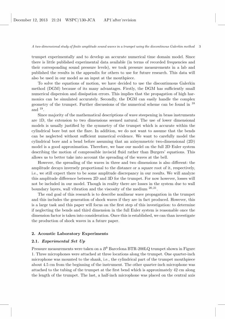
Pressure measurements were taken on a Bb Barcelona BTR-200LQ trumpet shown in Figure
1. Three microphones were attached at three locations along the trumpet. One quarter-inch
microphone was mounted to the shank, i.e., the cylindrical part of the trumpet mouthpiece
about 4.5 cm from the beginning of the instrument. The other quarter-inch microphone was
attached to the tubing of the trumpet at the first bend which is approximately 42 cm along
the length of the trumpet. The last, a half-inch microphone was placed on the central axis

December 12, 2013 21:24 WSPC/130-JCA AP1˙after˙revision
4 J. Resch, L. Krivodonova & J. Vanderkooy
of the trumpet approximately 16 cm - 17 cm outside the bell. In the rest of the paper, we
will refer to these locations as mouthpiece, bend, and bell.
Fig. 1: Placement of microphones on the Barcelona BTR-200LQ trumpet.
To mount the microphones at the mouthpiece and bend, small holes were cut into
the cylindrical part of the mouthpiece and trumpet bore. Quarter inch o-ring compression
fittings were then soldered to the trumpet bore over these holes. In an attempt not to alter
the acoustic properties of the trumpet, the microphones were placed so that the diaphragms
made the boundary of the tube as smooth as possible. The microphones were connected
to three inputs of an Agilent four channel digital oscilloscope and the pressure data from
all three microphones was collected simultaneously while the instrument was held in the
normal playing position. The data was captured once the note of choice was steady and
only a couple of periods of the raw data was saved into the local computer.
The Agilent digital oscilloscope quantizes the input signals with 8-bit converters, so we
might expect the microphone data to have a maximum of 256 levels. However, due to the
large oversampling of the internal converters, many samples are added together to produce
output samples with much better resolution. We found that our data displayed over 2000
levels, so it was captured with 11-bit precision, having a signal-to-noise ratio of about 66
dB.
In order to make the path of the airflow more direct we avoided using the valves of
the Bb trumpet. For this reason, we chose to play C3 and C4 notes, which correspond to
a concert Bb3 and Bb
4, respectively. Both of these notes were played forte (f ), which means
loud.
2.2. Experimental Results
One period of the recorded pressure measurements for the Bb3 and Bb
4 notes played f is
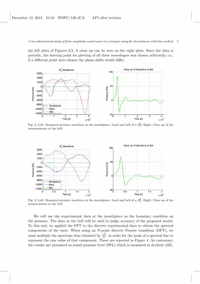
depicted in the left plots of Figures 2 and 3, respectively. The plots show deviation of the
sound wave pressure from atmospheric pressure, which is 101325 Pa. Since the pressure at
the bell is much lower than inside the instrument, its waveform looks like a straight line in
December 12, 2013 21:24 WSPC/130-JCA AP1˙after˙revision
A two-dimensional study of finite amplitude sound waves in a trumpet using the discontinous Galerkin method 5
the left plots of Figures 2-3. A close up can be seen on the right plots. Since the data is
periodic, the starting point for plotting of all three waveshapes was chosen arbitrarily, i.e.,
if a different point were chosen the phase shifts would differ.
Fig. 2: Left: Measured pressure waveform at the mouthpiece, bend and bell of a Bb3. Right: Close up of the
measurements at the bell.
Fig. 3: Left: Measured pressure waveform at the mouthpiece, bend and bell of a Bb4. Right: Close up of the
measurements at the bell.
We will use the experimental data at the mouthpiece as the boundary condition on
the pressure. The data at the bell will be used to judge accuracy of the proposed model.
To this end, we applied the FFT to the discrete experimental data to obtain the spectral
components of the wave. When using an N-point discrete Fourier transform (DFT), we
must multiply the spectrum thus obtained by√
2N , in order for the peak of a spectral line to
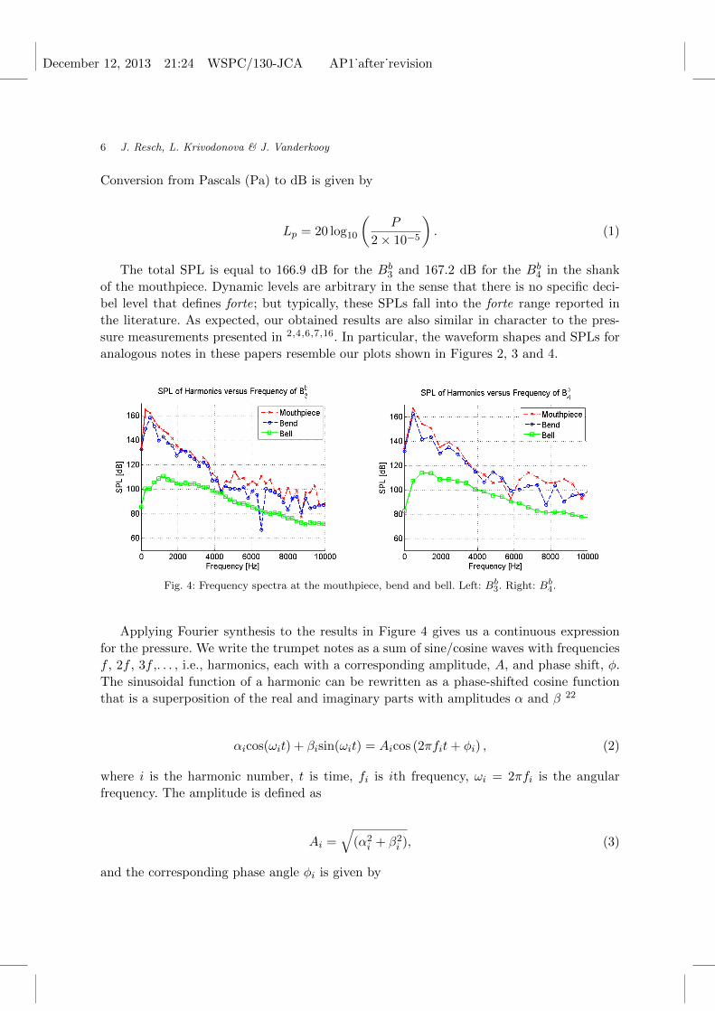
represent the rms value of that component. These are reported in Figure 4. As customary,
the results are presented as sound pressure level (SPL) which is measured in decibels (dB).
December 12, 2013 21:24 WSPC/130-JCA AP1˙after˙revision
6 J. Resch, L. Krivodonova & J. Vanderkooy
Conversion from Pascals (Pa) to dB is given by
Lp = 20 log10
(P
2× 10⁻⁵
). (1)
The total SPL is equal to 166.9 dB for the Bb3 and 167.2 dB for the Bb
4 in the shank
of the mouthpiece. Dynamic levels are arbitrary in the sense that there is no specific deci-
bel level that defines forte; but typically, these SPLs fall into the forte range reported in
the literature. As expected, our obtained results are also similar in character to the pres-
sure measurements presented in 2,4,6,7,16. In particular, the waveform shapes and SPLs for
analogous notes in these papers resemble our plots shown in Figures 2, 3 and 4.
Fig. 4: Frequency spectra at the mouthpiece, bend and bell. Left: Bb3. Right: Bb
4.
Applying Fourier synthesis to the results in Figure 4 gives us a continuous expression
for the pressure. We write the trumpet notes as a sum of sine/cosine waves with frequencies
f , 2f , 3f ,. . . , i.e., harmonics, each with a corresponding amplitude, A, and phase shift, φ.
The sinusoidal function of a harmonic can be rewritten as a phase-shifted cosine function
that is a superposition of the real and imaginary parts with amplitudes α and β 22
αicos(ωit) + βisin(ωit) = Aicos (2πfit+ φi) , (2)
where i is the harmonic number, t is time, fi is ith frequency, ωi = 2πfi is the angular
frequency. The amplitude is defined as
Ai =√
(α2i + β2
i ), (3)
and the corresponding phase angle φi is given by
December 12, 2013 21:24 WSPC/130-JCA AP1˙after˙revision
A two-dimensional study of finite amplitude sound waves in a trumpet using the discontinous Galerkin method 7
φi = arctan
(βiαi
). (4)
Therefore, one period of the entire pressure waveform of a desired note is expressed as
p = A0 +
N/2∑i
2Aicos (2πfit+ φi) , (5)
where A0 is the term corresponding to the direct current, and N is the number of points
in our data, and fN/2 is the Nyquist frequency. The amplitude is multiplied by a factor of
two since the Ai are double-sided.
3. Numerical Set Up
3.1. Number of Harmonics
Next, we need to determine how many harmonics in (5) are required in order to reconstruct
and accurately describe a pressure waveform for a given note. We obtained slightly more than
200 harmonics from our FFT analysis. Not all of these frequencies are meaningful. Once the
SPLs drop by approximately 50 dB, these frequencies represent noise in our measurements.
Our oscilloscope had a dynamic range of 66 dB, so it does not contribute to the noise in
our measurements. The number of retained harmonics is important as it influences the size
of the mesh: we normally require a minimum number of mesh cells per wavelength in order
to resolve it properly. This number depends on the order of the numerical scheme.
In early investigations, it was typical for only six to eight harmonics to be considered in
describing a note, e.g., 2,3,6. We found, however, that more harmonics are necessary for an
accurate representation of a note at the mouthpiece and an even higher number for mea-
surements taken outside the bell. This is in line with recent results in the literature 23. The
required number of harmonics depend on the acoustical system and available computational
resources. In order to find the proper number, we truncate the FFT reconstruction (5) at
Nf = 5, 10, 15, 20, 25, and 30 number of harmonics and measure the resulting error (Table
1). The relative error was measured in the L2 norm
error(%) =‖pFFT − pTrun‖2‖pFFT ‖2
∗ 100%, (6)
where pFFT is the fully reconstructed waveform and pTrun is the reconstruction truncated
after a given number of harmonics. We observe that for the mouthpiece at least fifteen
harmonics are necessary to describe Bb3 and at least ten are needed for Bb
4. Adding extra
frequencies does not significantly reduce the error. The difference in the number of harmonics
for Bb3 and Bb
4 can be explained by looking at the waveforms in Figures 2-3 where the Bb4
December 12, 2013 21:24 WSPC/130-JCA AP1˙after˙revision
8 J. Resch, L. Krivodonova & J. Vanderkooy
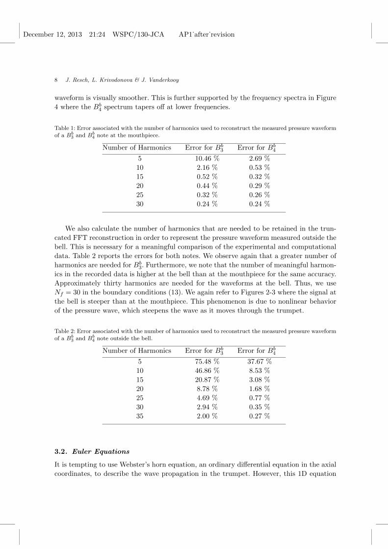
waveform is visually smoother. This is further supported by the frequency spectra in Figure
4 where the Bb4 spectrum tapers off at lower frequencies.
Table 1: Error associated with the number of harmonics used to reconstruct the measured pressure waveformof a Bb
3 and Bb4 note at the mouthpiece.
Number of Harmonics Error for Bb3 Error for Bb
4
5 10.46 % 2.69 %
10 2.16 % 0.53 %
15 0.52 % 0.32 %
20 0.44 % 0.29 %
25 0.32 % 0.26 %
30 0.24 % 0.24 %
We also calculate the number of harmonics that are needed to be retained in the trun-
cated FFT reconstruction in order to represent the pressure waveform measured outside the
bell. This is necessary for a meaningful comparison of the experimental and computational
data. Table 2 reports the errors for both notes. We observe again that a greater number of
harmonics are needed for Bb3. Furthermore, we note that the number of meaningful harmon-
ics in the recorded data is higher at the bell than at the mouthpiece for the same accuracy.
Approximately thirty harmonics are needed for the waveforms at the bell. Thus, we use
Nf = 30 in the boundary conditions (13). We again refer to Figures 2-3 where the signal at
the bell is steeper than at the mouthpiece. This phenomenon is due to nonlinear behavior
of the pressure wave, which steepens the wave as it moves through the trumpet.
Table 2: Error associated with the number of harmonics used to reconstruct the measured pressure waveformof a Bb
3 and Bb4 note outside the bell.
Number of Harmonics Error for Bb3 Error for Bb
4
5 75.48 % 37.67 %
10 46.86 % 8.53 %
15 20.87 % 3.08 %
20 8.78 % 1.68 %
25 4.69 % 0.77 %
30 2.94 % 0.35 %
35 2.00 % 0.27 %
3.2. Euler Equations
It is tempting to use Webster’s horn equation, an ordinary differential equation in the axial
coordinates, to describe the wave propagation in the trumpet. However, this 1D equation
December 12, 2013 21:24 WSPC/130-JCA AP1˙after˙revision
A two-dimensional study of finite amplitude sound waves in a trumpet using the discontinous Galerkin method 9
is inadequate for our purposes. The method neglects the nonlinear coupling of the forward
and backward moving waves. Furthermore, the pressure field is assumed to be uniform
throughout the width of the duct and the flare expansion of the bell has to be gradual. If
the rate of change of the flare is too large, this method fails even for low frequency waves
because we cannot decouple the modes 13. To describe nonlinear wave propagation in the
trumpet for loud, high frequency notes, it is essential to take the pressure variations and
mode coupling into consideration without placing any restrictions on the flare of the bell.
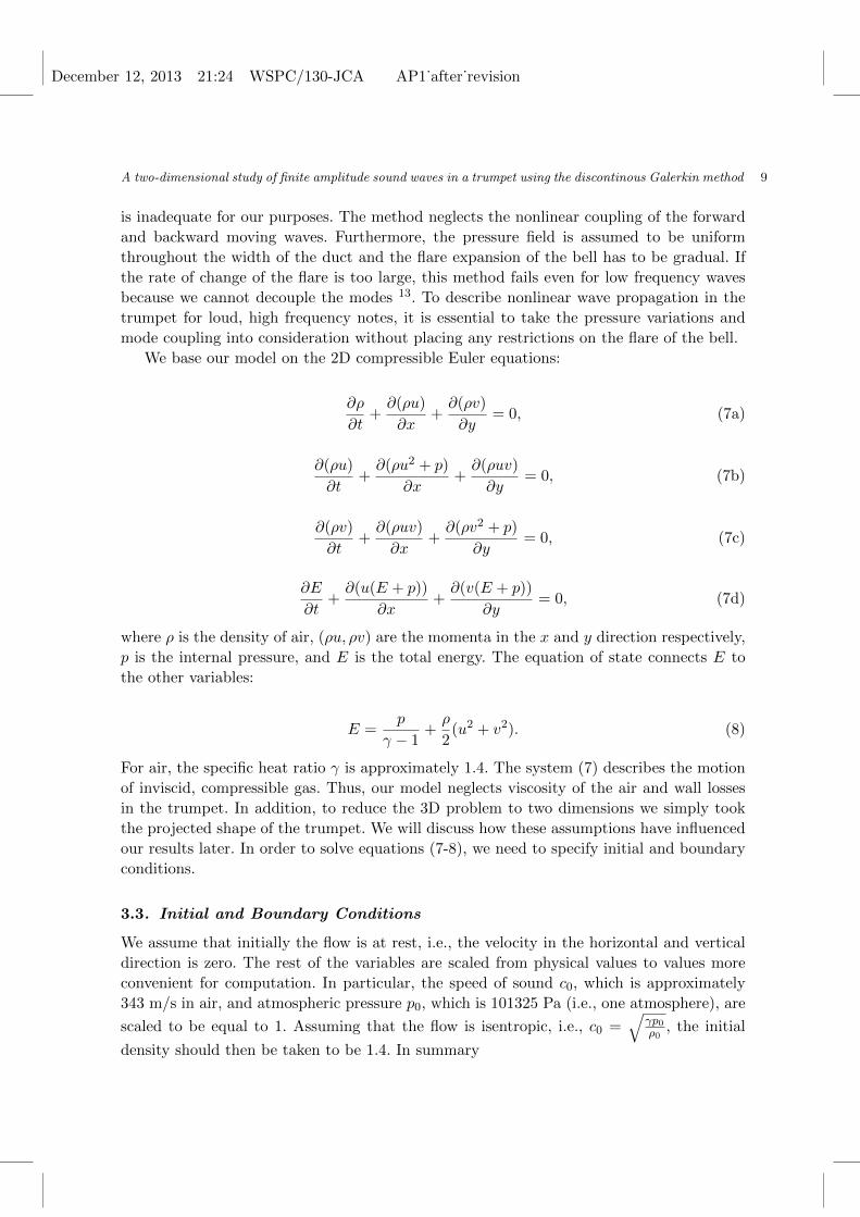
We base our model on the 2D compressible Euler equations:
∂ρ
∂t+∂(ρu)
∂x+∂(ρv)
∂y= 0, (7a)
∂(ρu)
∂t+∂(ρu2 + p)
∂x+∂(ρuv)
∂y= 0, (7b)
∂(ρv)
∂t+∂(ρuv)
∂x+∂(ρv2 + p)
∂y= 0, (7c)
∂E
∂t+∂(u(E + p))
∂x+∂(v(E + p))
∂y= 0, (7d)
where ρ is the density of air, (ρu, ρv) are the momenta in the x and y direction respectively,
p is the internal pressure, and E is the total energy. The equation of state connects E to
the other variables:
E =p
γ − 1+ρ
2(u2 + v2). (8)
For air, the specific heat ratio γ is approximately 1.4. The system (7) describes the motion
of inviscid, compressible gas. Thus, our model neglects viscosity of the air and wall losses
in the trumpet. In addition, to reduce the 3D problem to two dimensions we simply took
the projected shape of the trumpet. We will discuss how these assumptions have influenced
our results later. In order to solve equations (7-8), we need to specify initial and boundary
conditions.
3.3. Initial and Boundary Conditions
We assume that initially the flow is at rest, i.e., the velocity in the horizontal and vertical
direction is zero. The rest of the variables are scaled from physical values to values more
convenient for computation. In particular, the speed of sound c0, which is approximately
343 m/s in air, and atmospheric pressure p0, which is 101325 Pa (i.e., one atmosphere), are
scaled to be equal to 1. Assuming that the flow is isentropic, i.e., c0 =√
γp0ρ0
, the initial
density should then be taken to be 1.4. In summary
December 12, 2013 21:24 WSPC/130-JCA AP1˙after˙revision
10 J. Resch, L. Krivodonova & J. Vanderkooy
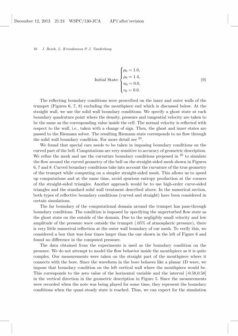
Initial State:
p0 = 1.0,
ρ0 = 1.4,
u0 = 0.0,
v0 = 0.0.
(9)
The reflecting boundary conditions were prescribed on the inner and outer walls of the
trumpet (Figures 6, 7, 8) excluding the mouthpiece end which is discussed below. At the
straight wall, we use the solid wall boundary conditions. We specify a ghost state at each
boundary quadrature point where the density, pressure and tangential velocity are taken to
be the same as the corresponding value inside the cell. The normal velocity is reflected with
respect to the wall, i.e., taken with a change of sign. Then, the ghost and inner states are
passed to the Riemann solver. The resulting Riemann state corresponds to no flow through
the solid wall boundary condition. For more detail see 24.
We found that special care needs to be taken in imposing boundary conditions on the
curved part of the bell. Computations are very sensitive to accuracy of geometric description.
We refine the mesh and use the curvature boundary conditions proposed in 25 to simulate
the flow around the curved geometry of the bell on the straight-sided mesh shown in Figures
6, 7 and 8. Curved boundary conditions take into account the curvature of the true geometry
of the trumpet while computing on a simpler straight-sided mesh. This allows us to speed
up computations and at the same time, avoid spurious entropy production at the corners
of the straight-sided triangles. Another approach would be to use high-order curve-sided
triangles and the standard solid wall treatment described above. In the numerical section,
both types of reflective boundary conditions (curved and straight) have been considered in
certain simulations.
The far boundary of the computational domain around the trumpet has pass-through
boundary conditions. The condition is imposed by specifying the unperturbed flow state as
the ghost state on the outside of the domain. Due to the negligibly small velocity and low
amplitude of the pressure wave outside the trumpet (.05% of atmospheric pressure), there
is very little numerical reflection at the outer wall boundary of our mesh. To verify this, we
considered a box that was four times larger than the one shown in the left of Figure 6 and
found no difference in the computed pressure.
The data obtained from the experiments is used as the boundary condition on the
pressure. We do not attempt to model the flow behavior inside the mouthpiece as it is quite
complex. Our measurements were taken on the straight part of the mouthpiece where it
connects with the bore. Since the waveform in the bore behaves like a planar 1D wave, we
impose that boundary condition on the left vertical wall where the mouthpiece would be.
This corresponds to the zero value of the horizontal variable and the interval [-0.58,0.58]
in the vertical direction in the geometric description in Figure 5. Since the measurements
were recorded when the note was being played for some time, they represent the boundary
conditions when the quasi steady state is reached. Thus, we can expect for the simulation
December 12, 2013 21:24 WSPC/130-JCA AP1˙after˙revision
A two-dimensional study of finite amplitude sound waves in a trumpet using the discontinous Galerkin method 11
that the first time the wave transverses the trumpet, the output will not be accurate.
However, if simulations are performed correctly, then the reflected waves should fit well
with the prescribed values at the wall as they form the standing wave pattern.
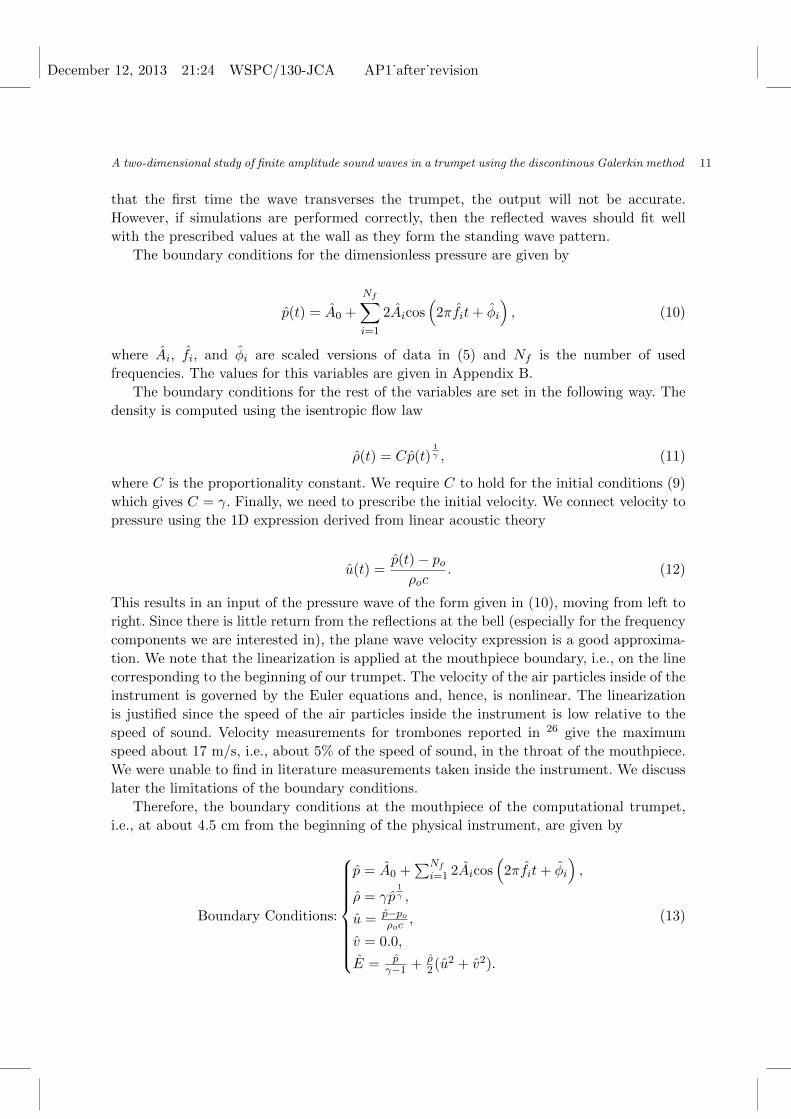
The boundary conditions for the dimensionless pressure are given by
p(t) = A0 +
Nf∑i=1
2Aicos(
2πfit+ φi
), (10)
where Ai, fi, and φi are scaled versions of data in (5) and Nf is the number of used
frequencies. The values for this variables are given in Appendix B.
The boundary conditions for the rest of the variables are set in the following way. The
density is computed using the isentropic flow law
ρ(t) = Cp(t)1γ , (11)
where C is the proportionality constant. We require C to hold for the initial conditions (9)
which gives C = γ. Finally, we need to prescribe the initial velocity. We connect velocity to
pressure using the 1D expression derived from linear acoustic theory
u(t) =p(t)− poρoc
. (12)
This results in an input of the pressure wave of the form given in (10), moving from left to
right. Since there is little return from the reflections at the bell (especially for the frequency
components we are interested in), the plane wave velocity expression is a good approxima-
tion. We note that the linearization is applied at the mouthpiece boundary, i.e., on the line
corresponding to the beginning of our trumpet. The velocity of the air particles inside of the
instrument is governed by the Euler equations and, hence, is nonlinear. The linearization
is justified since the speed of the air particles inside the instrument is low relative to the
speed of sound. Velocity measurements for trombones reported in 26 give the maximum
speed about 17 m/s, i.e., about 5% of the speed of sound, in the throat of the mouthpiece.
We were unable to find in literature measurements taken inside the instrument. We discuss
later the limitations of the boundary conditions.
Therefore, the boundary conditions at the mouthpiece of the computational trumpet,
i.e., at about 4.5 cm from the beginning of the physical instrument, are given by
Boundary Conditions:
p = A0 +∑Nf
i=1 2Aicos(
2πfit+ φi
),
ρ = γp1γ ,
u = p−poρoc
,
v = 0.0,
E = pγ−1 + ρ
2(u2 + v2).
(13)
December 12, 2013 21:24 WSPC/130-JCA AP1˙after˙revision
12 J. Resch, L. Krivodonova & J. Vanderkooy
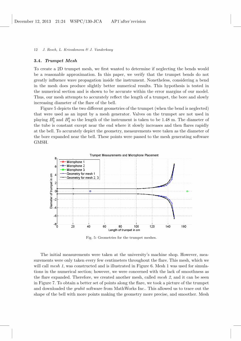
3.4. Trumpet Mesh
To create a 2D trumpet mesh, we first wanted to determine if neglecting the bends would
be a reasonable approximation. In this paper, we verify that the trumpet bends do not
greatly influence wave propagation inside the instrument. Nonetheless, considering a bend
in the mesh does produce slightly better numerical results. This hypothesis is tested in
the numerical section and is shown to be accurate within the error margins of our model.
Thus, our mesh attempts to accurately reflect the length of a trumpet, the bore and slowly
increasing diameter of the flare of the bell.
Figure 5 depicts the two different geometries of the trumpet (when the bend is neglected)
that were used as an input by a mesh generator. Valves on the trumpet are not used in
playing Bb3 and Bb
4 so the length of the instrument is taken to be 1.48 m. The diameter of
the tube is constant except near the end where it slowly increases and then flares rapidly
at the bell. To accurately depict the geometry, measurements were taken as the diameter of
the bore expanded near the bell. These points were passed to the mesh generating software
GMSH.
Fig. 5: Geometries for the trumpet meshes.
The initial measurements were taken at the university’s machine shop. However, mea-
surements were only taken every few centimeters throughout the flare. This mesh, which we
will call mesh 1, was constructed and is illustrated in Figure 6. Mesh 1 was used for simula-
tions in the numerical section; however, we were concerned with the lack of smoothness as
the flare expanded. Therefore, we created another mesh, called mesh 2, and it can be seen
in Figure 7. To obtain a better set of points along the flare, we took a picture of the trumpet
and downloaded the grabit software from MathWorks Inc.. This allowed us to trace out the
shape of the bell with more points making the geometry more precise, and smoother. Mesh
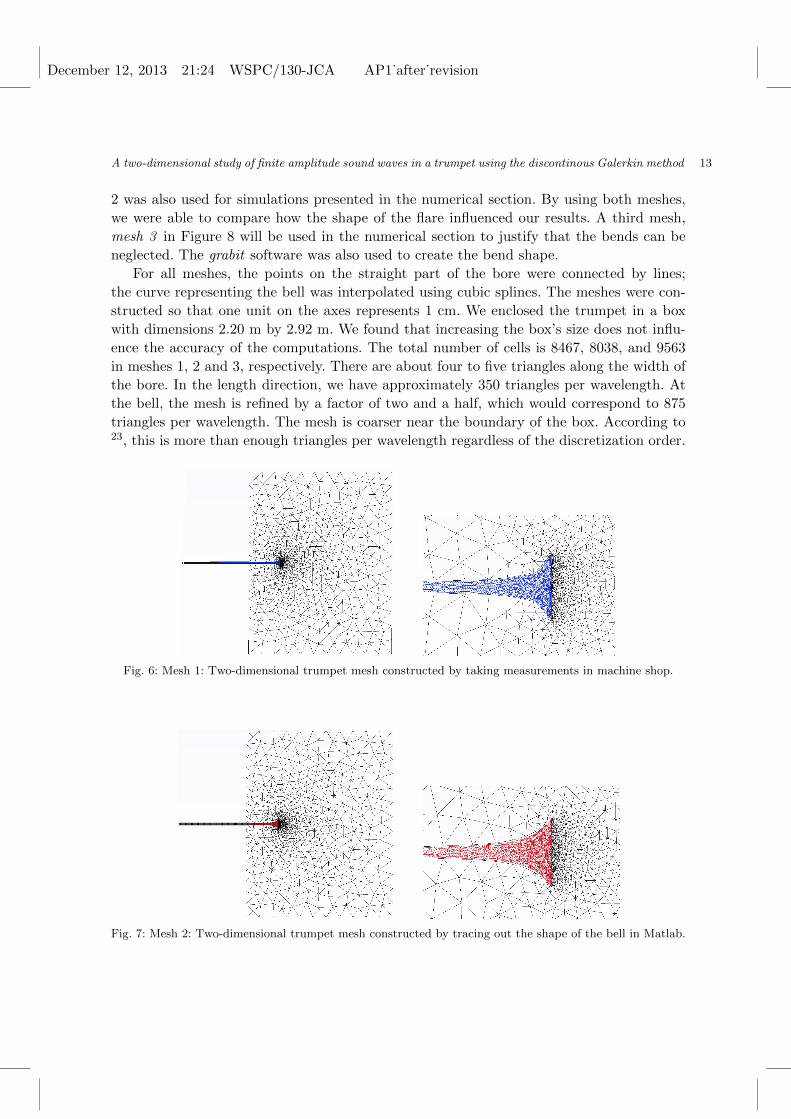
December 12, 2013 21:24 WSPC/130-JCA AP1˙after˙revision
A two-dimensional study of finite amplitude sound waves in a trumpet using the discontinous Galerkin method 13
2 was also used for simulations presented in the numerical section. By using both meshes,
we were able to compare how the shape of the flare influenced our results. A third mesh,
mesh 3 in Figure 8 will be used in the numerical section to justify that the bends can be
neglected. The grabit software was also used to create the bend shape.
For all meshes, the points on the straight part of the bore were connected by lines;
the curve representing the bell was interpolated using cubic splines. The meshes were con-
structed so that one unit on the axes represents 1 cm. We enclosed the trumpet in a box
with dimensions 2.20 m by 2.92 m. We found that increasing the box’s size does not influ-
ence the accuracy of the computations. The total number of cells is 8467, 8038, and 9563
in meshes 1, 2 and 3, respectively. There are about four to five triangles along the width of
the bore. In the length direction, we have approximately 350 triangles per wavelength. At
the bell, the mesh is refined by a factor of two and a half, which would correspond to 875
triangles per wavelength. The mesh is coarser near the boundary of the box. According to23, this is more than enough triangles per wavelength regardless of the discretization order.
Fig. 6: Mesh 1: Two-dimensional trumpet mesh constructed by taking measurements in machine shop.
Fig. 7: Mesh 2: Two-dimensional trumpet mesh constructed by tracing out the shape of the bell in Matlab.
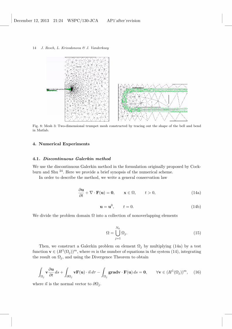
December 12, 2013 21:24 WSPC/130-JCA AP1˙after˙revision
14 J. Resch, L. Krivodonova & J. Vanderkooy
Fig. 8: Mesh 3: Two-dimensional trumpet mesh constructed by tracing out the shape of the bell and bendin Matlab.
4. Numerical Experiments
4.1. Discontinuous Galerkin method
We use the discontinuous Galerkin method in the formulation originally proposed by Cock-
burn and Shu 24. Here we provide a brief synopsis of the numerical scheme.
In order to describe the method, we write a general conservation law
∂u
∂t+∇ · F(u) = 0, x ∈ Ω, t > 0, (14a)
u = u0, t = 0. (14b)
We divide the problem domain Ω into a collection of nonoverlapping elements
Ω =
Nh⋃j=1
Ωj . (15)
Then, we construct a Galerkin problem on element Ωj by multiplying (14a) by a test
function v ∈ (H1(Ωj))m, where m is the number of equations in the system (14), integrating
the result on Ωj , and using the Divergence Theorem to obtain
∫Ωj
v∂u
∂tds+
∫∂Ωj
vF(u) · ~n dτ −∫
Ωj
gradv · F(u) ds = 0, ∀v ∈ (H1(Ωj))m, (16)
where ~n is the normal vector to ∂Ωj .
December 12, 2013 21:24 WSPC/130-JCA AP1˙after˙revision
A two-dimensional study of finite amplitude sound waves in a trumpet using the discontinous Galerkin method 15
The solution u is approximated by a vector function Uj = (Uj,1, Uj,2, . . . , Uj,m)T , where
Uj,k =
Np∑i=1
cj,k,iϕi, k = 1, 2, . . . ,m, (17)
in a finite-dimensional subspace of the solution space. The basis ϕiNpi=1 is chosen to be
orthonormal in L2(Ωj)18. This will produce a multiple of the identity for the mass matrix
on Ωj when the testing function v is chosen to be equal to the basis functions consecutively
starting with ϕ1.
Due to the discontinuous nature of the numerical solution, the normal flux Fn = F(u) ·~n, is not defined on ∂Ωj . The usual strategy is to define it in terms of a numerical flux
Fn(Uj ,Uk) that depends on the solution Uj on Ωj and Uk on the neighboring element
Ωk sharing the portion of the boundary ∂Ωjk common to both elements. In our numerical
experiments, we have used the Roe numerical flux 18. Finally, the L2 volume and surface
inner products in (16) are computed using 2p and 2p+ 1 order accurate Gauss quadratures18, respectively, where p is the order of the orthonormal basis. The resulting system of ODEs
is
dc
dt= f(c), (18)
where c is the vector of unknowns and f is a nonlinear vector function resulting from the
boundary and volume integrals in (16).
Numerical experiments presented in Section 4.3 were computed using a linear basis and
verified by running the same tests with a quadratic basis. Due to the very fine meshes used,
the results were extremely similar.
4.2. Estimated Difference of Trumpet Output in Two and Three
Dimensions
In that portion of the trumpet where the bore diameter is constant, the acoustic signal is
essentially 1D. We can approximately compare the 2D simulations with 3D measurements
if we make a few reasonable assumptions about the acoustic signals leaving the bell. Let
us compare a 3D trumpet of bore with radius R with a 2D trumpet of the same projected
shape. We choose our 2D trumpet with a height W such that the area of its rectangular
bore is the same as that of the 3D trumpet, thus 2RW = πR2. Using the measured acoustic
pressure for our simulations means that the same total power is traveling down the actual
trumpet and the simulation.
Now consider that most of the acoustic power will leave each trumpet bell, since much
of the power is in the higher harmonics. We assume that this will be similar in 2D and
3D, i.e., we are using a conservation of energy argument. In addition, we assume that the
axial acoustic pressure2 measured in similar places outside the bell is proportional to the
December 12, 2013 21:24 WSPC/130-JCA AP1˙after˙revision
16 J. Resch, L. Krivodonova & J. Vanderkooy
total power leaving the instrument. There will be some differences in 2D and 3D but we
will assume that they are not significant relative to the other considerations.
The acoustic waves leaving the bell in both 2D and 3D will have curved wavefronts, and
we can equate the pressure2 times the wavefront area so that the power leaving each bell
is the same. It is necessary to estimate (see Appendix A) these curved wavefront areas, the
one in 2D being a curved strip of width h bridging the edges of the bell, and the one in 3D
being a spherical cap bounded by the edge of the bell. If A2 and A3 represent these areas,
and p2 and p3 represent the simulated and measured axial pressures on these areas, then
we would set p22A2 = p2
3A3.
There is one more detail needed to compare the simulated and measured pressures. They
have been assessed not at the bell but some distance from it, due to the original placement
of the microphone well outside the bell. In comparing this position to the one on the curved
wavefront bridging the bell, we must account for the different variation of amplitude with
distance in 2D and 3D. In 2D, the amplitude is closely proportional to 1√r, whereas in 3D
the amplitude varies as 1r . We need to know where the center of curvature is located for the
wavefronts. All these considerations have been included in the numerical factor of 14 dB
difference between 2D and 3D at a distance 16 cm from the bell. While the whole process
seems a bit rudimentary, it nonetheless allows a comparison between 2D and 3D.
4.3. Computational Results
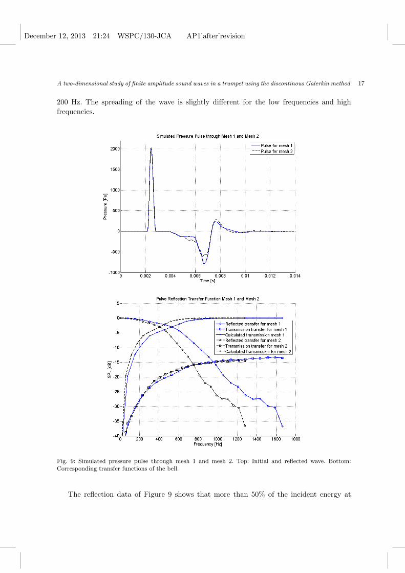
To better interpret our simulation results, we first examine the acoustic behavior of the 2D
bell. We send down the trumpet a pulse given by
p1 =
1.0 + (0.01− 0.01 cos(1500 t)), if t < 2π
1500
1.0, else
which corresponds to a pressure pulse with an amplitude of approximately 2000 Pa. Since the
amplitude is only 2% of an atmosphere, we can view the pulse as linear. We do not observe
wave steepening. In the top plot of Figure 9, we show the pressure simulated at a point
located at the mid-length of the cylindrical bore. The first peak located at approximately
t = 0.0025 corresponds to the initial pulse moving from the mouthpiece towards the bell.
The second inverted peak seen at about t = 0.007 corresponds to the signal traveling back
to the mouthpiece after it has been reflected at the bell.
The reflected transfer data of Figure 9 (bottom), is calculated from the frequency content
of the reflected pulse divided by that of the incident pulse. This curve represents the power
reflected by the bell meshes. The calculated transmission data, which is the compliment of
the reflected transfer data, represent the power transmitted from the bell; the transmission
transfer data are the output of the bell meshes. The curves representing the output of the
bell meshes have a reduction in the sound pressure level (SPL). This is mainly because the
wave spreads as it exits the bell. However, we can see that the shape of the calculated and
simulated transmission data are similar, especially for frequency components greater than
December 12, 2013 21:24 WSPC/130-JCA AP1˙after˙revision
A two-dimensional study of finite amplitude sound waves in a trumpet using the discontinous Galerkin method 17
200 Hz. The spreading of the wave is slightly different for the low frequencies and high
frequencies.
Fig. 9: Simulated pressure pulse through mesh 1 and mesh 2. Top: Initial and reflected wave. Bottom:Corresponding transfer functions of the bell.
The reflection data of Figure 9 shows that more than 50% of the incident energy at
December 12, 2013 21:24 WSPC/130-JCA AP1˙after˙revision
18 J. Resch, L. Krivodonova & J. Vanderkooy
the mouthpiece is transmitted out of the bell for frequencies above about 600 Hz for mesh
1, and 400 Hz for mesh 2. This is where the reflection plot crosses at -3 dB (in 3D, we
expect that where the plot crosses will increase in frequency). This means, in theory, that
frequency components less than approximately 600 Hz and 400 Hz, for mesh 1 and mesh 2
respectively, are mostly reflected before or within the bell. We hypothesize that the 200 Hz
difference is due to the variation of the bell curvature. For mesh 1, the bell is not as smooth
and along the length of the instrument, the flare widens further down the tube compared
to mesh 2. For mesh 1, this will cause more of the frequency components to stay within the
confines of the duct. This would explain why the pulse for mesh 1 in Figure 9 (bottom) has
a lower peak relative to mesh 2. As the frequency increases, the wave travels further into
the bell. For frequency components greater than roughly 1000 Hz, the waves are not being
reflected at all and we see that the transmission data matches for both meshes in Figure
9 (bottom). This is to be expected since both mesh 1 and 2 have the same geometry by
the time the bell is fully flared. We will use these findings in the discussion of our trumpet
simulations.
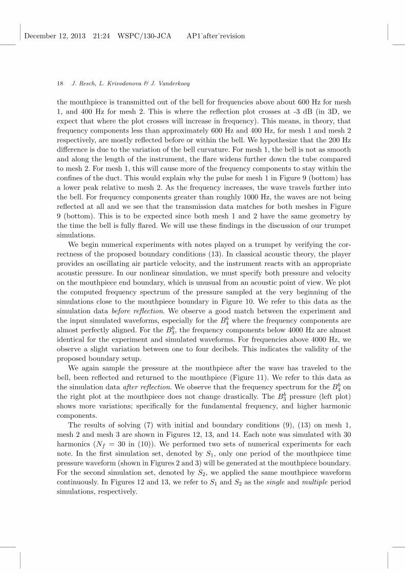
We begin numerical experiments with notes played on a trumpet by verifying the cor-
rectness of the proposed boundary conditions (13). In classical acoustic theory, the player
provides an oscillating air particle velocity, and the instrument reacts with an appropriate
acoustic pressure. In our nonlinear simulation, we must specify both pressure and velocity
on the mouthpiece end boundary, which is unusual from an acoustic point of view. We plot
the computed frequency spectrum of the pressure sampled at the very beginning of the
simulations close to the mouthpiece boundary in Figure 10. We refer to this data as the
simulation data before reflection. We observe a good match between the experiment and
the input simulated waveforms, especially for the Bb4 where the frequency components are
almost perfectly aligned. For the Bb3, the frequency components below 4000 Hz are almost
identical for the experiment and simulated waveforms. For frequencies above 4000 Hz, we
observe a slight variation between one to four decibels. This indicates the validity of the
proposed boundary setup.
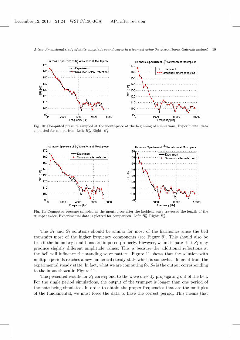
We again sample the pressure at the mouthpiece after the wave has traveled to the
bell, been reflected and returned to the mouthpiece (Figure 11). We refer to this data as
the simulation data after reflection. We observe that the frequency spectrum for the Bb4 on
the right plot at the mouthpiece does not change drastically. The Bb3 pressure (left plot)
shows more variations; specifically for the fundamental frequency, and higher harmonic
components.
The results of solving (7) with initial and boundary conditions (9), (13) on mesh 1,
mesh 2 and mesh 3 are shown in Figures 12, 13, and 14. Each note was simulated with 30
harmonics (Nf = 30 in (10)). We performed two sets of numerical experiments for each
note. In the first simulation set, denoted by S1, only one period of the mouthpiece time
pressure waveform (shown in Figures 2 and 3) will be generated at the mouthpiece boundary.
For the second simulation set, denoted by S2, we applied the same mouthpiece waveform
continuously. In Figures 12 and 13, we refer to S1 and S2 as the single and multiple period
simulations, respectively.
December 12, 2013 21:24 WSPC/130-JCA AP1˙after˙revision
A two-dimensional study of finite amplitude sound waves in a trumpet using the discontinous Galerkin method 19
Fig. 10: Computed pressure sampled at the mouthpiece at the beginning of simulations. Experimental datais plotted for comparison. Left: Bb
3. Right: Bb4.
Fig. 11: Computed pressure sampled at the mouthpiece after the incident wave traversed the length of thetrumpet twice. Experimental data is plotted for comparison. Left: Bb
3. Right: Bb4.
The S1 and S2 solutions should be similar for most of the harmonics since the bell
transmits most of the higher frequency components (see Figure 9). This should also be
true if the boundary conditions are imposed properly. However, we anticipate that S2 may
produce slightly different amplitude values. This is because the additional reflections at
the bell will influence the standing wave pattern. Figure 11 shows that the solution with
multiple periods reaches a new numerical steady state which is somewhat different from the
experimental steady state. In fact, what we are computing for S2 is the output corresponding
to the input shown in Figure 11.
The presented results for S1 correspond to the wave directly propagating out of the bell.
For the single period simulations, the output of the trumpet is longer than one period of
the note being simulated. In order to obtain the proper frequencies that are the multiples
of the fundamental, we must force the data to have the correct period. This means that
December 12, 2013 21:24 WSPC/130-JCA AP1˙after˙revision
20 J. Resch, L. Krivodonova & J. Vanderkooy
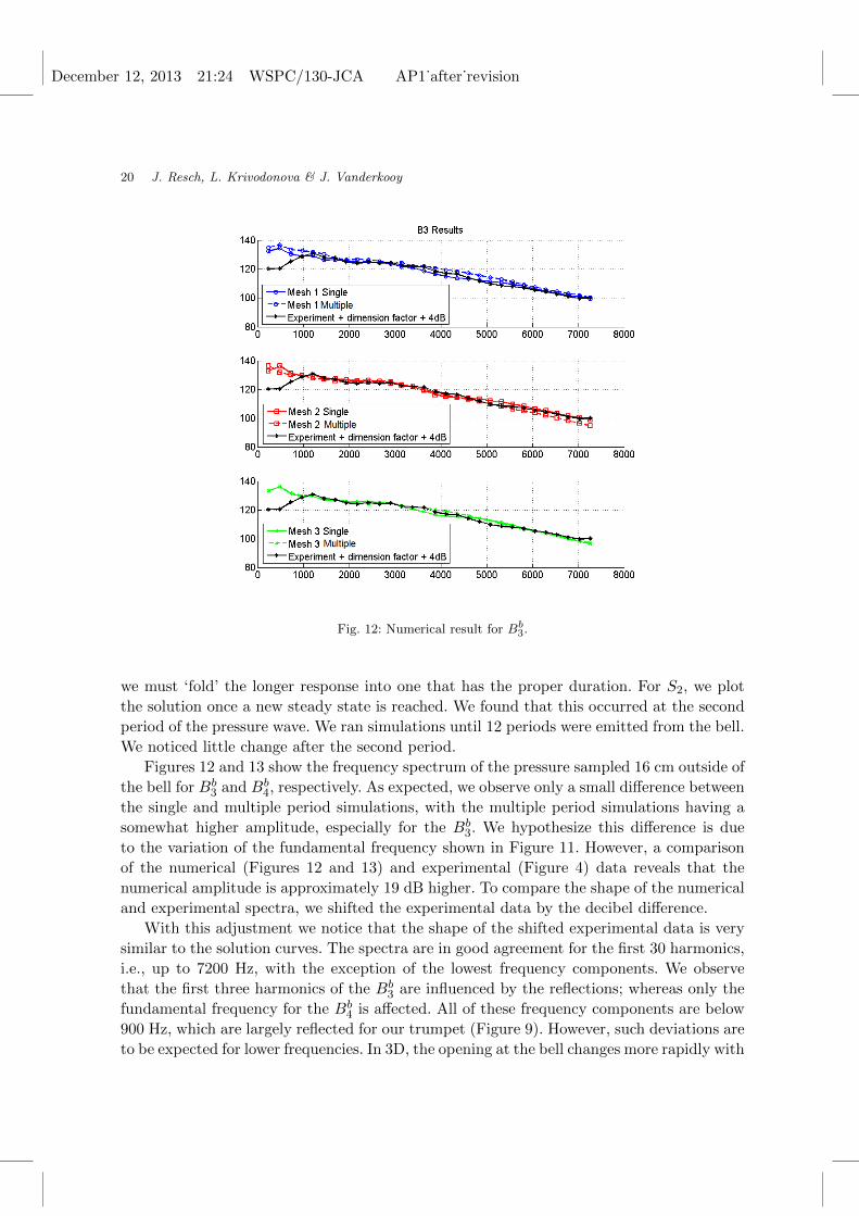
Fig. 12: Numerical result for Bb3.
we must ‘fold’ the longer response into one that has the proper duration. For S2, we plot
the solution once a new steady state is reached. We found that this occurred at the second
period of the pressure wave. We ran simulations until 12 periods were emitted from the bell.
We noticed little change after the second period.
Figures 12 and 13 show the frequency spectrum of the pressure sampled 16 cm outside of
the bell for Bb3 and Bb
4, respectively. As expected, we observe only a small difference between
the single and multiple period simulations, with the multiple period simulations having a
somewhat higher amplitude, especially for the Bb3. We hypothesize this difference is due
to the variation of the fundamental frequency shown in Figure 11. However, a comparison
of the numerical (Figures 12 and 13) and experimental (Figure 4) data reveals that the
numerical amplitude is approximately 19 dB higher. To compare the shape of the numerical
and experimental spectra, we shifted the experimental data by the decibel difference.
With this adjustment we notice that the shape of the shifted experimental data is very
similar to the solution curves. The spectra are in good agreement for the first 30 harmonics,
i.e., up to 7200 Hz, with the exception of the lowest frequency components. We observe
that the first three harmonics of the Bb3 are influenced by the reflections; whereas only the
fundamental frequency for the Bb4 is affected. All of these frequency components are below
900 Hz, which are largely reflected for our trumpet (Figure 9). However, such deviations are
to be expected for lower frequencies. In 3D, the opening at the bell changes more rapidly with
December 12, 2013 21:24 WSPC/130-JCA AP1˙after˙revision
A two-dimensional study of finite amplitude sound waves in a trumpet using the discontinous Galerkin method 21
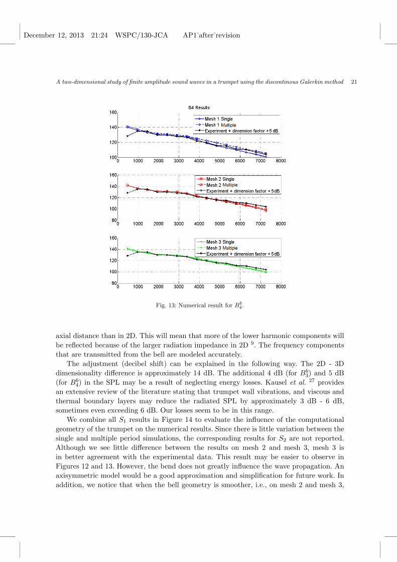
Fig. 13: Numerical result for Bb4.
axial distance than in 2D. This will mean that more of the lower harmonic components will
be reflected because of the larger radiation impedance in 2D 9. The frequency components
that are transmitted from the bell are modeled accurately.
The adjustment (decibel shift) can be explained in the following way. The 2D - 3D
dimensionality difference is approximately 14 dB. The additional 4 dB (for Bb3) and 5 dB
(for Bb4) in the SPL may be a result of neglecting energy losses. Kausel et al. 27 provides
an extensive review of the literature stating that trumpet wall vibrations, and viscous and
thermal boundary layers may reduce the radiated SPL by approximately 3 dB - 6 dB,
sometimes even exceeding 6 dB. Our losses seem to be in this range.
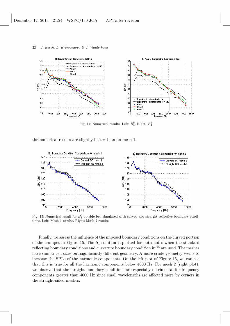
We combine all S1 results in Figure 14 to evaluate the influence of the computational
geometry of the trumpet on the numerical results. Since there is little variation between the
single and multiple period simulations, the corresponding results for S2 are not reported.
Although we see little difference between the results on mesh 2 and mesh 3, mesh 3 is
in better agreement with the experimental data. This result may be easier to observe in
Figures 12 and 13. However, the bend does not greatly influence the wave propagation. An
axisymmetric model would be a good approximation and simplification for future work. In
addition, we notice that when the bell geometry is smoother, i.e., on mesh 2 and mesh 3,
December 12, 2013 21:24 WSPC/130-JCA AP1˙after˙revision
22 J. Resch, L. Krivodonova & J. Vanderkooy
Fig. 14: Numerical results. Left: Bb3. Right: Bb
4
the numerical results are slightly better than on mesh 1.
Fig. 15: Numerical result for Bb3 outside bell simulated with curved and straight reflective boundary condi-
tions. Left: Mesh 1 results. Right: Mesh 2 results.
Finally, we assess the influence of the imposed boundary conditions on the curved portion
of the trumpet in Figure 15. The S1 solution is plotted for both notes when the standard
reflecting boundary conditions and curvature boundary condition in 25 are used. The meshes
have similar cell sizes but significantly different geometry. A more crude geometry seems to
increase the SPLs of the harmonic components. On the left plot of Figure 15, we can see
that this is true for all the harmonic components below 4000 Hz. For mesh 2 (right plot),
we observe that the straight boundary conditions are especially detrimental for frequency
components greater than 4000 Hz since small wavelengths are affected more by corners in
the straight-sided meshes.
December 12, 2013 21:24 WSPC/130-JCA AP1˙after˙revision
A two-dimensional study of finite amplitude sound waves in a trumpet using the discontinous Galerkin method 23
5. Conclusions
Overall, our results are encouraging. Figures 12, 13, and 14 show that the energy repre-
sented in the measured mouthpiece pressure (Figure 4) comes out of the bell producing
similar spectra. Although the 2D - 3D amplitude discrepancy can mostly be explained (see
Appendix A), 2D simulations are not adequate to simulate nonlinear wave propagation
within the trumpet. Neglecting the spreading of the wave in the third dimension is too sig-
nificant to dismiss. However, considering an axisymmetric 2D model could provide better
results.
In future work, we intend to determine a more accurate steady-state velocity for the
boundary condition at the mouthpiece. In principle, if we know the acoustic input impedance
of the trumpet mouthpiece, we could calculate the steady-state velocity that would accom-
pany the measured steady-state pressure. However, since the bell transmits most of the
energy above 800 Hz - 1000 Hz, we do not think the correction is too serious. The details
of this will be explored in future a paper.
More importantly, we plan to examine our model in three dimensions. From our current
results, we can say with confidence that the model and numerical method chosen is an
appropriate one. Therefore, we will continue using the discontinuous Galerkin method to
examine our 3D model. Until these simulations are complete, we will refrain from making
any comments on the generation of shock waves in the trumpet.
Appendix
A. Derivation of Dimension Factor
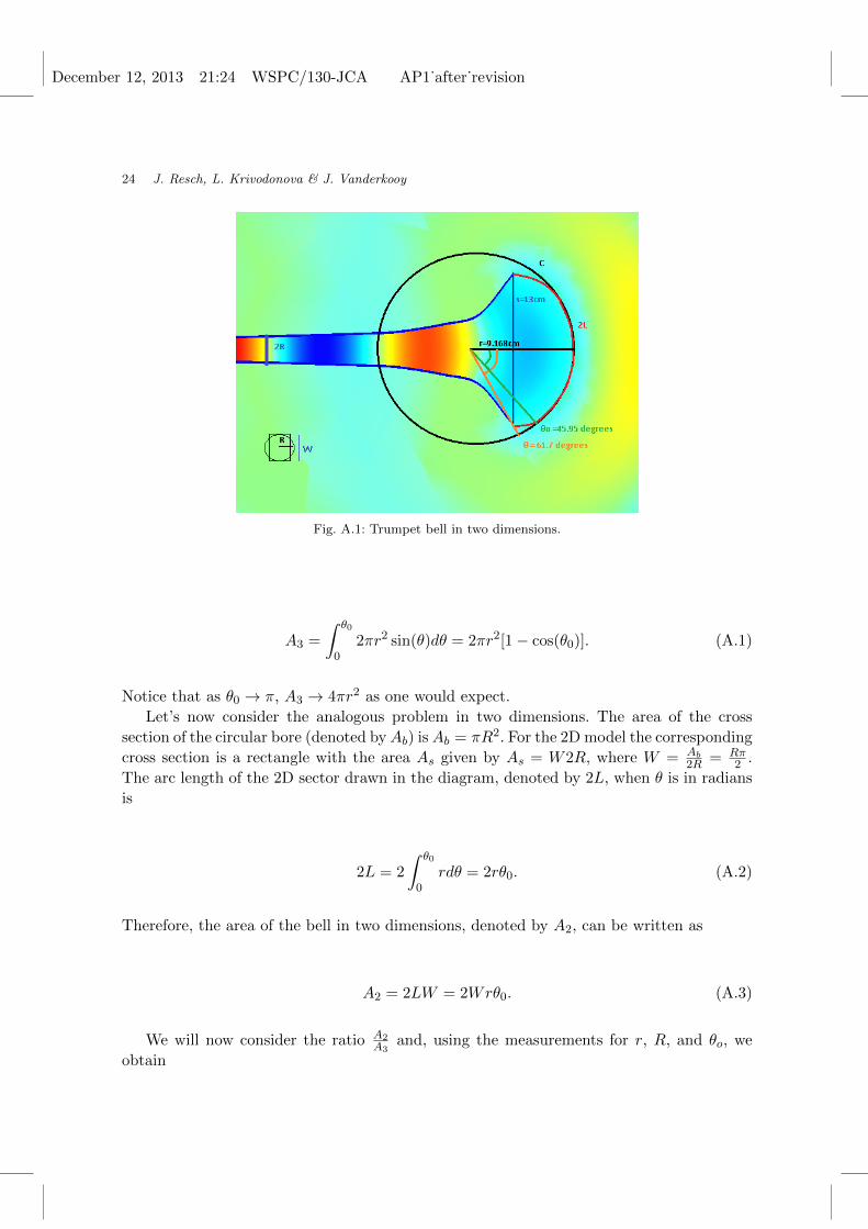
Consider the 2D trumpet bell depicted in Figure A.1. The diameter of the bell is denoted
by s (approximately 13 cm) and the radius of the bore is denoted by R (approximately
0.7 cm). We will simply assume that the pressure will be the same across the arc denoted
by L. In other words, we are assuming that the axial pressure in both 2D and 3D is a
good measure of the total energy leaving the bell (i.e., we are assuming that the total
energy leaving the bell is conserved). The radius of the arc will be denoted by r and was
determined by approximating the exiting wavefront by a circle C, with radius 9.168 cm.
Although this circle slightly overshoots the wavefront, it is the closest approximation. We
denote the angle θo ≈ 45.95o as the angle between the arc and the horizontal line r which
only considers the wavefront approximated by C. The angle θ0 can be found using
sin θ0 =s
2r,
which approximately gives θ0 = 0.793252 radians or 45.95 degrees.
We want to estimate the difference in the area of the curved wavefront propagating out
of the bell for the 2D and 3D problems. In three dimensions, we examine the area of the
cap, denoted by A3. This can be found by integrating a slice of the sector, i.e.,
December 12, 2013 21:24 WSPC/130-JCA AP1˙after˙revision
24 J. Resch, L. Krivodonova & J. Vanderkooy
Fig. A.1: Trumpet bell in two dimensions.
A3 =
∫ θ0
02πr2 sin(θ)dθ = 2πr2[1− cos(θ0)]. (A.1)
Notice that as θ0 → π, A3 → 4πr2 as one would expect.
Let’s now consider the analogous problem in two dimensions. The area of the cross
section of the circular bore (denoted byAb) isAb = πR2. For the 2D model the corresponding
cross section is a rectangle with the area As given by As = W2R, where W = Ab2R = Rπ
2 .
The arc length of the 2D sector drawn in the diagram, denoted by 2L, when θ is in radians
is
2L = 2
∫ θ0
0rdθ = 2rθ0. (A.2)
Therefore, the area of the bell in two dimensions, denoted by A2, can be written as
A2 = 2LW = 2Wrθ0. (A.3)
We will now consider the ratio A2A3
and, using the measurements for r, R, and θo, we
obtain
December 12, 2013 21:24 WSPC/130-JCA AP1˙after˙revision
A two-dimensional study of finite amplitude sound waves in a trumpet using the discontinous Galerkin method 25
A2
A3=
2Wrθ0
2πr2[1− cos(θ0)](A.4)
=Rθ0
2r[1− cos(θ0)]
≈ 0.1066.
A wavefront exiting the bell of a trumpet will do so with a certain amount of energy, that
should be conserved between the dimensions. Thus, we have
A3p23 = A2p
22 (A.5)(
p2
p3
)=
√A3
A2p2
p3≈ 3.13.
This gives the pressure ratio of p2p3≈ 3.13. Therefore, neglecting the third dimension in
our simulations could produce an amplitude that is 3.1 times larger than it should be for
the exiting wavefront, i.e., measured at 5 cm outside the bell. This corresponds to a SPL of
approximately 10 dB.
Next, we estimate what the difference in SPL will be when the wave is further outside
the bell. In two dimensions, the amplitude of the pressure waves (denoted by p2) will drop
off as a factor of 1√r
and in three dimensions pressure (denoted by p3) will drop off as 1r .
Therefore, the relationship between pressure at position a (denoted by pa) and pressure at
position b (denoted by pb) for two dimensions will be
p2,b
√b = p2,a
√a, (A.6)
and in three dimensions
p3,bb = p3,aa. (A.7)
Therefore, p2,b = (√a√b)p2,a and p3,b = (ab )p3,a. Considering the ratio between p2 and p3 gives
p2,b
p3,b= α
(p2,a
p3,a
)(A.8)
where α =√baa . In our case, α is approximately 1.5374 and p2
p3≈ 4.77. Therefore, we conclude
that the amplitude measured outside the bell will be approximately 14 dB too high.
December 12, 2013 21:24 WSPC/130-JCA AP1˙after˙revision
26 J. Resch, L. Krivodonova & J. Vanderkooy
B. Frequency Components
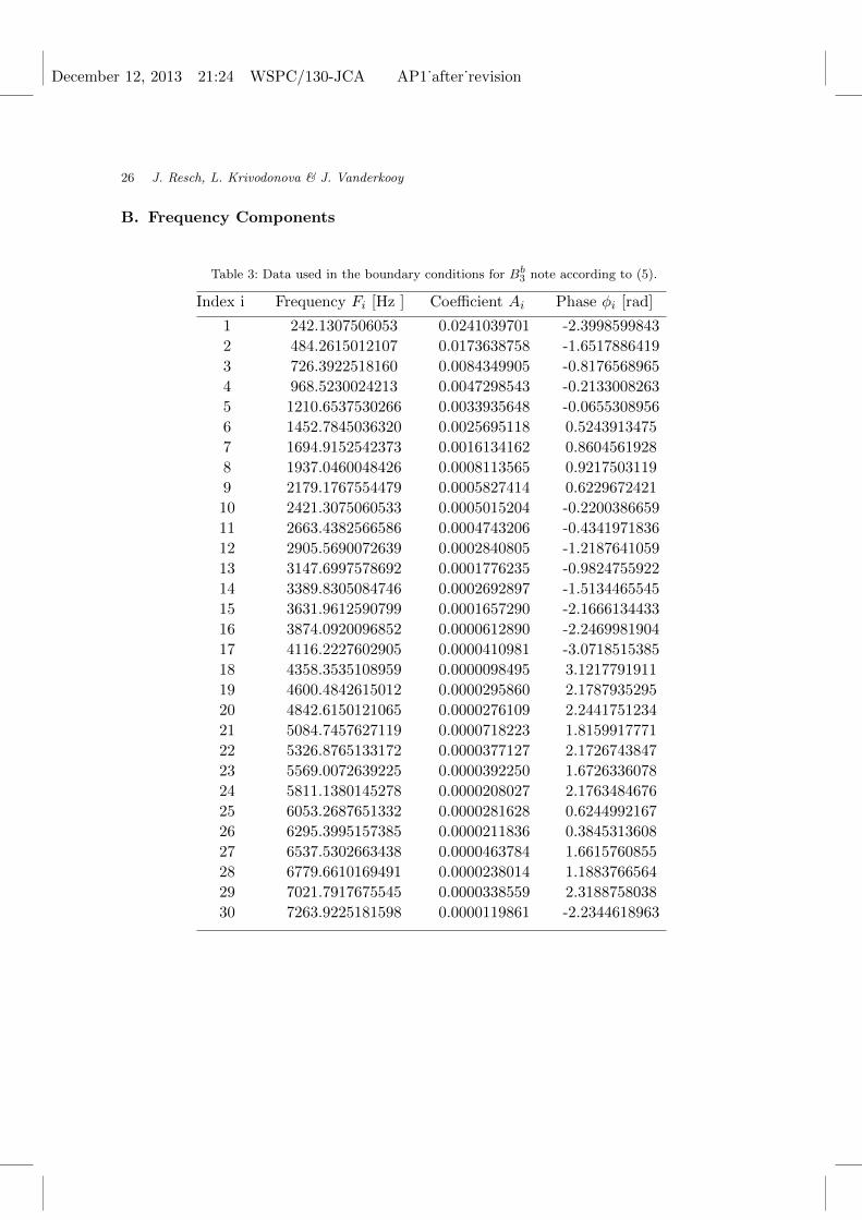
Table 3: Data used in the boundary conditions for Bb3 note according to (5).
Index i Frequency Fi [Hz ] Coefficient Ai Phase φi [rad]
1 242.1307506053 0.0241039701 -2.3998599843
2 484.2615012107 0.0173638758 -1.6517886419
3 726.3922518160 0.0084349905 -0.8176568965
4 968.5230024213 0.0047298543 -0.2133008263
5 1210.6537530266 0.0033935648 -0.0655308956
6 1452.7845036320 0.0025695118 0.5243913475
7 1694.9152542373 0.0016134162 0.8604561928
8 1937.0460048426 0.0008113565 0.9217503119
9 2179.1767554479 0.0005827414 0.6229672421
10 2421.3075060533 0.0005015204 -0.2200386659
11 2663.4382566586 0.0004743206 -0.4341971836
12 2905.5690072639 0.0002840805 -1.2187641059
13 3147.6997578692 0.0001776235 -0.9824755922
14 3389.8305084746 0.0002692897 -1.5134465545
15 3631.9612590799 0.0001657290 -2.1666134433
16 3874.0920096852 0.0000612890 -2.2469981904
17 4116.2227602905 0.0000410981 -3.0718515385
18 4358.3535108959 0.0000098495 3.1217791911
19 4600.4842615012 0.0000295860 2.1787935295
20 4842.6150121065 0.0000276109 2.2441751234
21 5084.7457627119 0.0000718223 1.8159917771
22 5326.8765133172 0.0000377127 2.1726743847
23 5569.0072639225 0.0000392250 1.6726336078
24 5811.1380145278 0.0000208027 2.1763484676
25 6053.2687651332 0.0000281628 0.6244992167
26 6295.3995157385 0.0000211836 0.3845313608
27 6537.5302663438 0.0000463784 1.6615760855
28 6779.6610169491 0.0000238014 1.1883766564
29 7021.7917675545 0.0000338559 2.3188758038
30 7263.9225181598 0.0000119861 -2.2344618963
December 12, 2013 21:24 WSPC/130-JCA AP1˙after˙revision
A two-dimensional study of finite amplitude sound waves in a trumpet using the discontinous Galerkin method 27
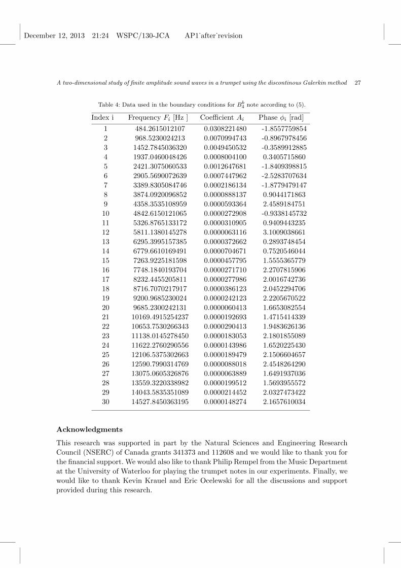
Table 4: Data used in the boundary conditions for Bb4 note according to (5).
Index i Frequency Fi [Hz ] Coefficient Ai Phase φi [rad]
1 484.2615012107 0.0308221480 -1.8557759854
2 968.5230024213 0.0070994743 -0.8967978456
3 1452.7845036320 0.0049450532 -0.3589912885
4 1937.0460048426 0.0008004100 0.3405715860
5 2421.3075060533 0.0012647681 -1.8409398815
6 2905.5690072639 0.0007447962 -2.5283707634
7 3389.8305084746 0.0002186134 -1.8779479147
8 3874.0920096852 0.0000888137 0.9044171863
9 4358.3535108959 0.0000593364 2.4589184751
10 4842.6150121065 0.0000272908 -0.9338145732
11 5326.8765133172 0.0000310905 0.9409443235
12 5811.1380145278 0.0000063116 3.1009038661
13 6295.3995157385 0.0000372662 0.2893748454
14 6779.6610169491 0.0000704671 0.7520546044
15 7263.9225181598 0.0000457795 1.5555365779
16 7748.1840193704 0.0000271710 2.2707815906
17 8232.4455205811 0.0000277986 2.0016742736
18 8716.7070217917 0.0000386123 2.0452294706
19 9200.9685230024 0.0000242123 2.2205670522
20 9685.2300242131 0.0000060413 1.6653082554
21 10169.4915254237 0.0000192693 1.4715414339
22 10653.7530266343 0.0000290413 1.9483626136
23 11138.0145278450 0.0000183053 2.1801855089
24 11622.2760290556 0.0000143986 1.6520225430
25 12106.5375302663 0.0000189479 2.1506604657
26 12590.7990314769 0.0000088018 2.4548264290
27 13075.0605326876 0.0000063889 1.6491937036
28 13559.3220338982 0.0000199512 1.5693955572
29 14043.5835351089 0.0000214452 2.0327473422
30 14527.8450363195 0.0000148274 2.1657610034
Acknowledgments
This research was supported in part by the Natural Sciences and Engineering Research
Council (NSERC) of Canada grants 341373 and 112608 and we would like to thank you for
the financial support. We would also like to thank Philip Rempel from the Music Department
at the University of Waterloo for playing the trumpet notes in our experiments. Finally, we
would like to thank Kevin Krauel and Eric Ocelewski for all the discussions and support
provided during this research.
December 12, 2013 21:24 WSPC/130-JCA AP1˙after˙revision
28 J. Resch, L. Krivodonova & J. Vanderkooy
References
1. D. T. Blackstock, M. F. Hamilton, & A. D. Pierce, Nonlinear Acoustics, edited by M. F. Hamiltonand D. T. Blackstock (Academic, San Diego, 1998).
2. A. J. Hirschberg, J. Gilbert, R. Msallam, & A. P. J. Wijnands, Shock waves in trombones, J.Acoust. Soc. Amer. 99 (1995) 1754-1758.
3. P. L. Rendon, D. Narezo, F. O. Bustamante, & A. P. Lopez, Nonlinear progressive waves in aslide trombone resonator, J. Acoust. Soc. Amer. 127 (2009) 1096-1103.
4. L. Norman. J. P. Chick, D. M. Campbell, A. Myers, & J. Gilbert, Player control of brassiness atintermediate dynamic levels in brass instruments,’ Acta Acustica united with Acustica 96 (2010)614-621.
5. J. Gilbert, D. M. Campbell, A. Myers, & R. W. Pyle, Differences between brass instrumentsarising from variations in brassiness due to nonlinear propagation, ISMA (2007).
6. J. Backus, & T. C. Hundley, Harmonic generation in the trumpet, J. Acoust. Soc. Amer. 49(1971) 509-519.
7. S. J. Elliott, & J.M. Bowsher, Regeneration in brass wind instrument, J. Sound and Vibration83 (1982) 181-217.
8. M. B. Lesser, & J. A. Lewis, Applications of matched asymptotic expansion methods to acoustics.Part 1. The Webster horn equation and the stepped duct, J. Acoust. Soc. Amer. 51 (1972) 1664-1669.
9. M. B. Lesser, & J. A. Lewis, Applications of matched asymptotic expansion methods to acoustics.Part 2. The open ended duct, J. Acoust. Soc. Amer. 52 (1972) 1406-1410.
10. E. Eisner Complete solutions of the ‘Webster’ horn equation J. Acoust. Soc. Amer. 41 (1967)1126-1146.
11. A. G. Webster, Acoustical impedance and the theory of horns and of the phonograph Proceedingsof the National Academy of Sciences of the United States of America 5 7 (1919) 275-282.
12. P. A. Martin, On Websters horn equation and some generalizations J. Acoust. Soc. Amer. 116(2004) 1381-1388.
13. V. Pagneux, N. Amir, & J. Kergomard, A study of wave propagation in varying crosssectionwaveguides by modal decomposition. Part I. Theory and validationJ. Acoust. Soc. Amer. 100(1996) 2034-2048.
14. J. W. Beauchamp, Analysis of simultaneous mouthpiece and output waveforms of wind instru-ments, in Audio Engineering Society Convention 66 - Audio Engineering Society (1980).
15. B. H. Pandya, G.S. Settles, & J. D. Miller, Schlieren imaging of shock waves in a trumpet, J.Acoust. Soc. Amer. 114 (2003) 3363-3367.
16. M. W. Thompson, & J. W. Strong, Inclusion of wave steepening in a frequency-domain modelof trombone sound production, J. Acoust. Soc. Amer. 110 (2001) 556-562.
17. J. Gilbert, L. Menguy, & M. Campbell, A simulation tool for brassiness studies, J. Acoust. Soc.Amer. 123 (2008) 1854.
18. J. E. Flaherty, L. Krivodonova, J. F. Remacle & M. S. Shephard, Some aspects of discontinuousGalerkin methods for hyperbolic conservation laws, J. Finite Elements in Analysis and Design38 (2002) 889-908.
19. A. Richter, J. Stiller, & R. Grundmann, Stablized discontinous Galerkin method for flow-soundinteraction, J. Comp. Acoust. 15 (2007) 123-143.
20. A. H. Benade, Fundamentals of Musical Acoustics (Dover Publications, New York, 1900).21. N. H. Fletcher, The nonlinear physics of musical instruments, Rep. Prog. Phys. 62 (1998) 723-
765.22. R. Feynman, The Feynman Lectures on Physics (California, 1990).23. A. Richter, Numerical investigations of the gas flow inside the bassoon, J. Fluids Eng. 134
December 12, 2013 21:24 WSPC/130-JCA AP1˙after˙revision
A two-dimensional study of finite amplitude sound waves in a trumpet using the discontinous Galerkin method 29
(2012).24. B. Cockburn & C. W. Shu, The Runge-Kutta discontinuous Galerkin finite element method for
conservation laws V: Multidimensional systems, J. Comp. Phys. 141 (1998) 119-224.25. L. Krivodonova & M. Berger, High-order Accurate Implementation of Solid Wall Boundary
Conditions in Curved Geometries, J. Comp. Phys. 38 (2002) 492–512.26. N. H. Fletcher, & T. D. Rossing, The Physics of Musical Instruments (Springer-Verlag, New
York, 1991).27. W. Kausel, & T. Moore, Influence of wall vibrations on the sound of brass wind instruments,
Universitat fur Musik und darstellende Kunst Weiin (2010) 1-46.