Embed Size (px)
Citation preview
1
Numerical simulation of finite amplitude standing waves in acoustic 1 resonators using finite volume method 2
3 Fangli Ninga,b*, Xiaofan Lic 4
5 a School of Mechanical Engineering, Northwestern Polytechnical University, 127 Youyi Xilu, Xi’an, Shaanxi, 6
China 7 b Department of Mechanical, Materials and Aerospace Engineering, Illinois Institute of Technology, 10 West 8
32nd Street, Chicago, Illinois, USA 9 10
c Department of Applied Mathematics, Illinois Institute of Technology, 10 West 32nd Street , Chicago, Illinois, 11 USA 12
13
* Corresponding author. Tel.: 1 312 567 8823 ; fax: 1 312 567 7230 E-‐mail address: [email protected]
2
Abstract 14
Finite amplitude standing waves in acoustic resonators are simulated. The fluid is initially at rest 15
and excited by a harmonic motion of the entire resonator. The unsteady compressible Navier-16
Stokes equations and the state equation for an ideal gas are employed. This study extends the 17
traditional pressure based finite volume SIMPLEC scheme for solving the equations without any 18
predefined standing waves. The pressure waveforms are computed in three different closed 19
resonators and two opened resonators. The studied shapes of resonators include cylinder, cone 20
and exponential horn. The numerical results obtained from the proposed finite volume method in 21
the study are in agreement with those obtained with the Galerkin method and the finite difference 22
method. We also investigate the velocity waveforms in the three different kinds of resonators, 23
and finds that the sharp velocity spikes appear at the ends of the resonator when the pressure has 24
shock-like waveform. The velocity in the closed conical resonator displays smooth harmonic 25
waveform. Finally, the pressure waveforms in opened resonators are simulated and analyzed. 26
The results show that the decrease in the ratio of the maximum to the minimum pressure at the 27
small end of the exponential resonator is less than that of cylindrical resonators when the flow 28
velocity at the opened end (relative to the resonator) is same. 29
Keywords: Nonlinear standing wave; Closed acoustic resonator; Opened acoustic resonator; Numerical 30
simulation; Finite volume method. 31
32
3
1. Introduction 33
High amplitude pressures in acoustic resonators can be very useful in many engineering 34
applications ranging from acoustic compression1, microfluidic devices2, to acoustic seal3. It has 35
been verified by both experiments and numerical simulations that high finite amplitude standing 36
wave pressures can be generated by oscillating acoustic resonators with axially variable cross-37
sectional areas (i.e. “shaped resonators”). In the experiments conducted by Lawrenson et al.1, 38
standing wave over-pressures in excess of 340% ambient pressure were reported. Li et al.4 39
numerically optimized the shapes of resonators for improving pressure compression ratio by 40
more than 241% at the same excitation forced by Lawrenson et al. 1 41
Studying the standing waves by real physical experiments would be expensive due to the 42
cost of constructing different resonator configurations. Hence, numerical simulation has become 43
an important tool for obtaining the nonlinear standing waves in acoustic resonators. Ilinskii et al.5 44
developed a simplified, one-dimensional nonlinear wave equation for the velocity potential in 45
shaped resonators. The velocity potential was expressed in a truncated finite Fourier series in 46
time based on the assumption that the nonlinear wave motion is periodic, and then the nonlinear 47
wave equation was reduced to a two-point boundary value problem. The one–dimensional model 48
was later improved by including the shear viscosity term in the conservation of momentum 49
equation6. 50
Erickson and Zinn7 employed the quasi-one-dimensional model derived in Ilinskii et al.5 and 51
neglected the third-order nonlinear terms. The velocity potential was expressed with a truncated 52
series of acoustic modes or trial functions with time-dependent amplitudes. Luo et al.8 also used 53
the Galerkin method to solve the quasi-one-dimensional model, but they modified the 54
momentum equations by inserting the simple forms of the shear viscosity term for a two-55
4
dimensional axisymmetric resonator and a three-dimensional low aspect-ratio rectangular 56
resonator. The Galerkin method was used to solve for the time-dependent amplitudes of the 57
acoustic modes in cylindrical resonators and exponential resonators. The eigenfunctions of the 58
acoustic resonators were chosen as the trial functions. Therefore, the algorithm was limited to 59
certain shaped resonators in which the eigenfunctions can be found analytically. 60
Vanhille and Campos-Pozuelo9 derived a second-order wave equation in Lagrangian 61
coordinates for the displacements in cylindrical resonators forced by an oscillating piston. The 62
displacements were assumed to be the sum of two terms, i.e., the linear solution plus a second-63
order correction, and then solved with a finite difference algorithm. Vanhill et al.10,11 further 64
employed a finite volume method(FVM) in space and a finite-difference scheme for time 65
derivatives to solve the nonlinear wave equation. Based on the assumption that the fluid is 66
irrotational, Vanhille and Campos-Pozuelo12,13 extended their finite difference model to the two 67
and three (included axisymmetric) dimensions. Independently, Chun and Kim14 solved nonlinear 68
standing waves in cylindrical and shaped resonators with the fourth-order compact finite 69
difference scheme. Based on a linear acoustic theory and fundamental fluid dynamics equations, 70
Hossian et al.15 developed a linear theory to estimate the resonant frequency and the standing 71
wave mode in closed exponential resonators and used finite difference MacCormack scheme for 72
simulating the finite amplitude standing waves. The proposed linear theory was limited to the 73
cylindrical and exponential resonators. Based on the linear wave equation, Yu et al.16 developed 74
a three-dimensional model for T-shaped acoustic resonators to predict the resonance frequencies 75
and then conducted experiments to validate the model. 76
Mortell and SeyMour17 used a Duffing-type perturbation to find the amplitude-frequency 77
relation, and then obtained shockless pressure waves in closed cone, horn and bulb resonators. 78
5
They also found that there are different frequency shift characters in the cone and bulb resonators. 79
Based on Lagrangian mechanics and perturbation for closed cylindrical resonators, Hamilton et 80
al.18 deduced the Webster horn equation for closed shaped resonators. In their study, the 81
efficiency of second-harmonic generation in modes determined the direction of the resonance 82
frequency shift. 83
Li and Raman19 reviewed the detailed information of the computational methods in 84
nonlinear standing waves in acoustic resonators. Most of the previous numerical studies were 85
limited to closed resonators and analyzed standing waves with a simplified approach: the 86
physical variables are assumed as finite sums of basic functions. In current study, we will 87
directly compute the formation of the standing waves in the closed resonators and opened 88
resonators starting from the initial position at rest without any predefined standing waves. To 89
achieve the goal, we use a pressure-based FVM for the unsteady compressible Navier-Stokes 90
equations without any other simplification. The SIMPLE-type method is a pressure-based FVM, 91
and was originally developed for incompressible flows20. Karki and Patankar21 substituted the 92
mass density correction by the pressure correction derived from the state equation, and then 93
successfully extended SIMPLE-type methods for solving steady viscous compressible flows at 94
all speeds. We employ similar idea of Karki and Patankar21, and extend the traditional SIMPLEC 95
scheme for solving unsteady viscous compressible flows in acoustic resonators. 96
This work will pave the way to compute the standing waves in resonators for acoustic seal. 97
Acoustic seal is a new application of the nonlinear standing waves in opened acoustic resonators 98
that requires complex boundary conditions, e.g., inlet flow, outlet flow and central blockages etc. 99
In this case, the standing waves cannot be predefined as a combination of harmonic components. 100
6
The study will provide a solid foundation for constructing successful future models for acoustic 101
seal. 102
The rest of the paper is organized as follows. In Sec. 2, we provide the basic equations for a 103
viscous compressible fluid and the boundary conditions of closed and opened resonators. In Sec. 104
3, we describe the pressure-based FVM. In Sec. 4, the FVM is used to simulate the standing 105
waves in closed resonators and opened resonators. Finally, we present our conclusions in Sec. 5. 106
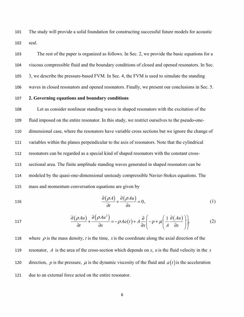
2. Governing equations and boundary conditions 107
Let us consider nonlinear standing waves in shaped resonators with the excitation of the 108
fluid imposed on the entire resonator. In this study, we restrict ourselves to the pseudo-one-109
dimensional case, where the resonators have variable cross sections but we ignore the change of 110
variables within the planes perpendicular to the axis of resonators. Note that the cylindrical 111
resonators can be regarded as a special kind of shaped resonators with the constant cross-112
sectional area. The finite amplitude standing waves generated in shaped resonators can be 113
modeled by the quasi-one-dimensional unsteady compressible Navier-Stokes equations. The 114
mass and momentum conversation equations are given by 115
( ) ( ) 0A Aut xρ ρ∂ ∂
+ =∂ ∂
, (1) 116
( ) ( ) ( ) ( )21AuAu Au
Aa t A pt x x A x
ρρρ µ
∂ ⎛ ⎞∂ ∂⎛ ⎞∂+ = − + − +⎜ ⎟⎜ ⎟⎜ ⎟∂ ∂ ∂ ∂⎝ ⎠⎝ ⎠, (2) 117
where ρ is the mass density, t is the time, x is the coordinate along the axial direction of the 118
resonator, A is the area of the cross-section which depends on x, u is the fluid velocity in the x 119
direction, p is the pressure, µ is the dynamic viscosity of the fluid and ( )a t is the acceleration 120
due to an external force acted on the entire resonator. 121
7
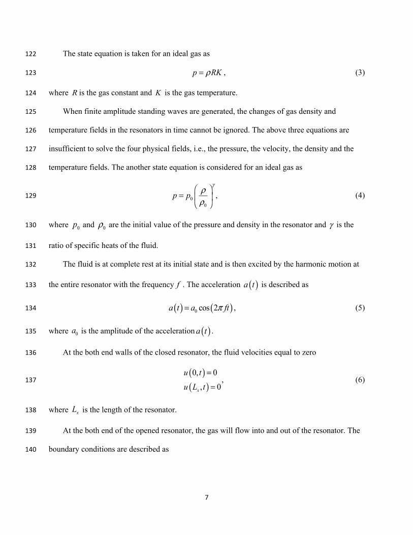
The state equation is taken for an ideal gas as 122
p RKρ= , (3) 123
where R is the gas constant and K is the gas temperature. 124
When finite amplitude standing waves are generated, the changes of gas density and 125
temperature fields in the resonators in time cannot be ignored. The above three equations are 126
insufficient to solve the four physical fields, i.e., the pressure, the velocity, the density and the 127
temperature fields. The another state equation is considered for an ideal gas as 128
00
p pγ
ρρ
⎛ ⎞= ⎜ ⎟
⎝ ⎠, (4) 129
where 0p and 0ρ are the initial value of the pressure and density in the resonator and γ is the 130
ratio of specific heats of the fluid. 131
The fluid is at complete rest at its initial state and is then excited by the harmonic motion at 132
the entire resonator with the frequency f . The acceleration ( )a t is described as 133
( ) ( )0 cos 2a t a ftπ= , (5) 134
where 0a is the amplitude of the acceleration ( )a t . 135
At the both end walls of the closed resonator, the fluid velocities equal to zero 136
( )( )0, 0
, 0x
u t
u L t
=
=, (6) 137
where xL is the length of the resonator. 138
At the both end of the opened resonator, the gas will flow into and out of the resonator. The 139
boundary conditions are described as 140
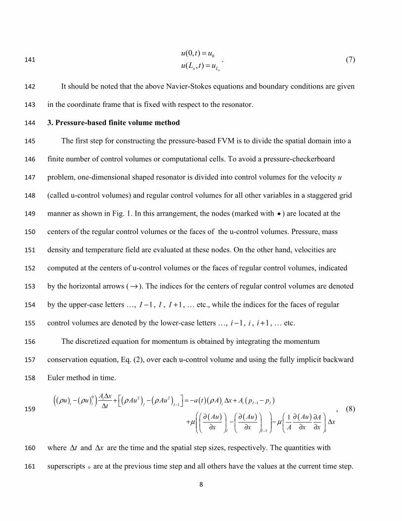
8
0(0, )( , )
xx L
u t uu L t u
==
. (7) 141
It should be noted that the above Navier-Stokes equations and boundary conditions are given 142
in the coordinate frame that is fixed with respect to the resonator. 143
3. Pressure-based finite volume method 144
The first step for constructing the pressure-based FVM is to divide the spatial domain into a 145
finite number of control volumes or computational cells. To avoid a pressure-checkerboard 146
problem, one-dimensional shaped resonator is divided into control volumes for the velocity u 147
(called u-control volumes) and regular control volumes for all other variables in a staggered grid 148
manner as shown in Fig. 1. In this arrangement, the nodes (marked with • ) are located at the 149
centers of the regular control volumes or the faces of the u-control volumes. Pressure, mass 150
density and temperature field are evaluated at these nodes. On the other hand, velocities are 151
computed at the centers of u-control volumes or the faces of regular control volumes, indicated 152
by the horizontal arrows (→ ). The indices for the centers of regular control volumes are denoted 153
by the upper-case letters …, 1I − , I , 1I + , … etc., while the indices for the faces of regular 154
control volumes are denoted by the lower-case letters …, 1i − , i , 1i + , … etc. 155
The discretized equation for momentum is obtained by integrating the momentum 156
conservation equation, Eq. (2), over each u-control volume and using the fully implicit backward 157
Euler method in time. 158
( ) ( )( ) ( ) ( ) ( )( ) ( )
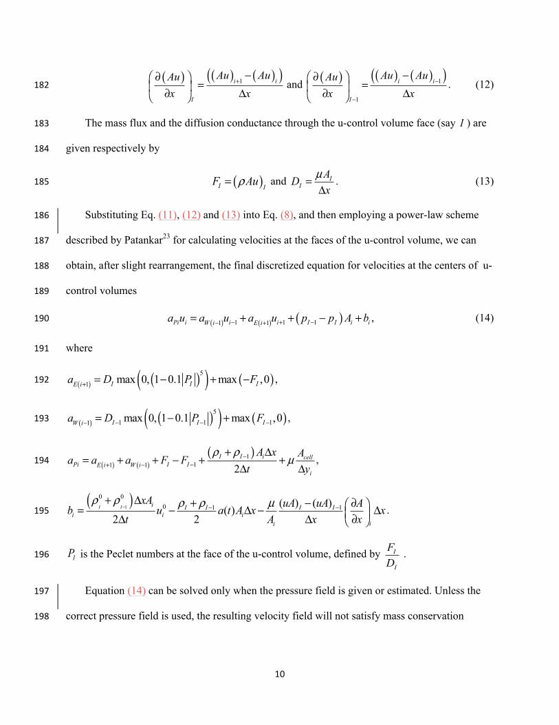
( ) ( ) ( )
0 2 211
1
1
ii I Ii i iI I
I I i
A xu u Au Au a t A x A p pt
Au Au Au A xx x A x x
ρ ρ ρ ρ ρ
µ µ
−−
−
Δ ⎡ ⎤− + − = − Δ + −⎣ ⎦Δ⎛ ⎞∂ ∂ ∂⎛ ⎞ ⎛ ⎞ ⎛ ⎞∂+ − − Δ⎜ ⎟⎜ ⎟ ⎜ ⎟ ⎜ ⎟⎜ ⎟∂ ∂ ∂ ∂⎝ ⎠ ⎝ ⎠ ⎝ ⎠⎝ ⎠
, (8) 159
where tΔ and xΔ are the time and the spatial step sizes, respectively. The quantities with 160
superscripts 0 are at the previous time step and all others have the values at the current time step. 161
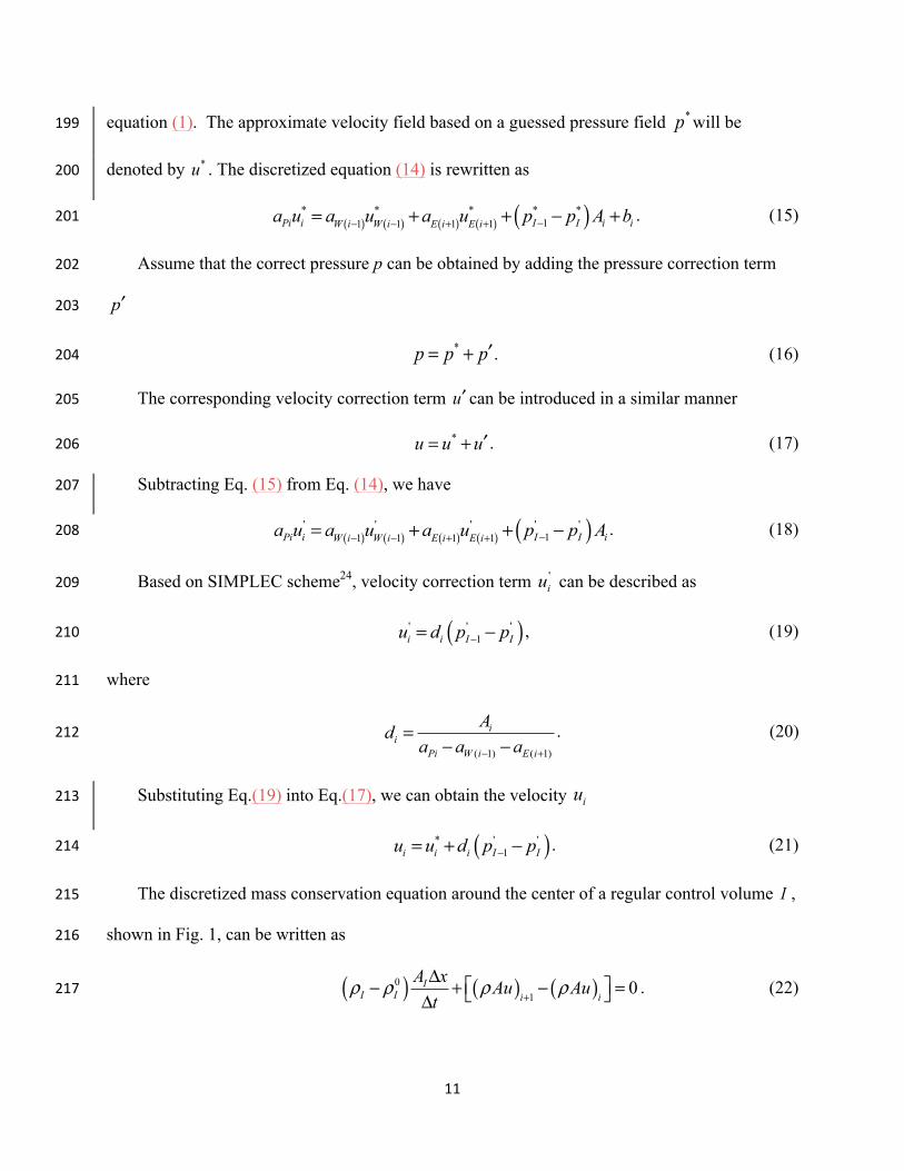
9
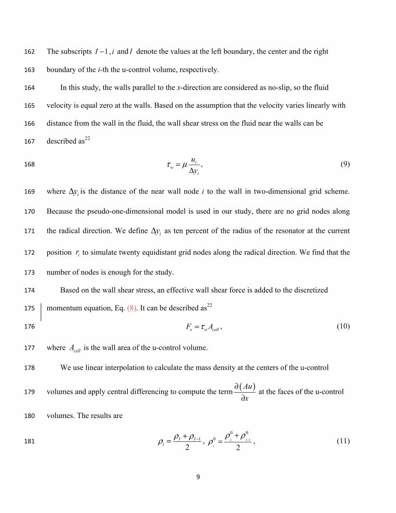
The subscripts 1I − , i and I denote the values at the left boundary, the center and the right 162
boundary of the i-th the u-control volume, respectively. 163
In this study, the walls parallel to the x-direction are considered as no-slip, so the fluid 164
velocity is equal zero at the walls. Based on the assumption that the velocity varies linearly with 165
distance from the wall in the fluid, the wall shear stress on the fluid near the walls can be 166
described as22 167
iw
i
uy
τ µ=Δ
, (9) 168
where is the distance of the near wall node i to the wall in two-dimensional grid scheme. 169
Because the pseudo-one-dimensional model is used in our study, there are no grid nodes along 170
the radical direction. We define as ten percent of the radius of the resonator at the current 171
position to simulate twenty equidistant grid nodes along the radical direction. We find that the 172
number of nodes is enough for the study. 173
Based on the wall shear stress, an effective wall shear force is added to the discretized 174
momentum equation, Eq. (8). It can be described as22 175
s w cellF Aτ= , (10) 176
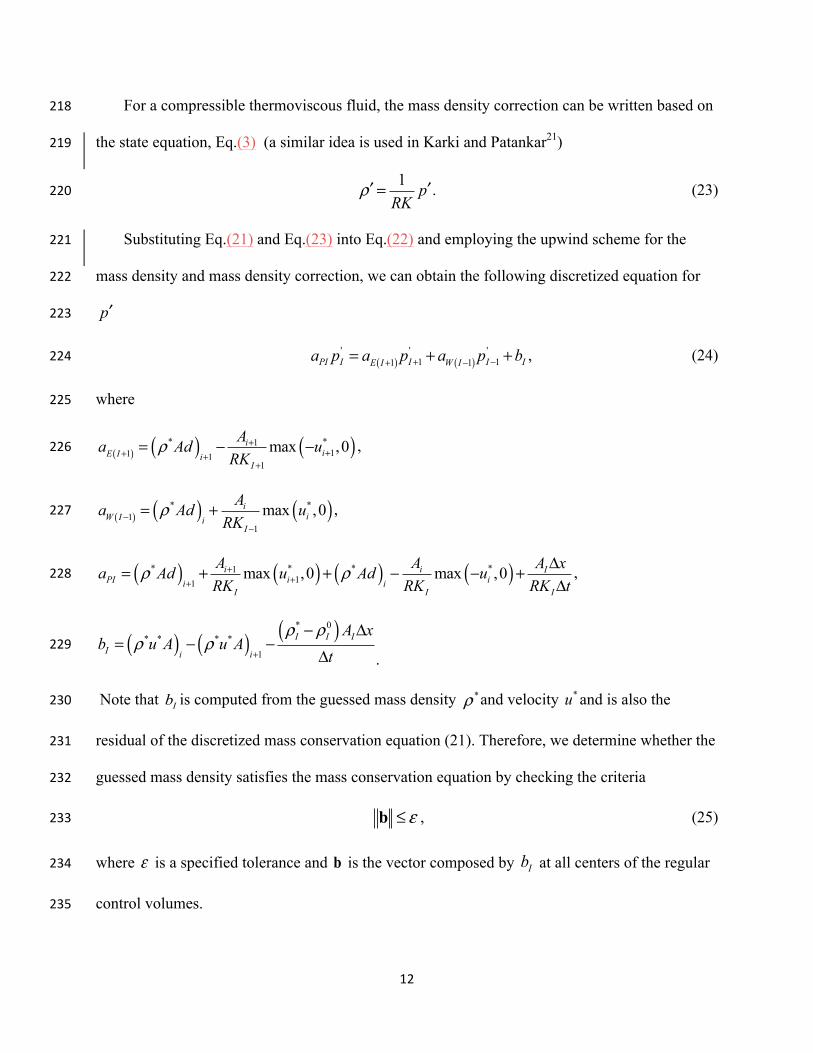
where cellA is the wall area of the u-control volume. 177
We use linear interpolation to calculate the mass density at the centers of the u-control 178
volumes and apply central differencing to compute the term ( )Aux
∂∂
at the faces of the u-control 179
volumes. The results are 180
1
2I I
iρ ρρ −+= , 1
0 00
2I I
i
ρ ρρ −
+= , (11) 181
iyΔ
iyΔ
ir
10
( ) ( ) ( )( )1i i
I
Au AuAux x
+−∂⎛ ⎞
=⎜ ⎟∂ Δ⎝ ⎠ and ( ) ( ) ( )( )1
1
i i
I
Au AuAux x
−
−
−∂⎛ ⎞=⎜ ⎟∂ Δ⎝ ⎠
. (12) 182
The mass flux and the diffusion conductance through the u-control volume face (say I ) are 183
given respectively by 184
( )I IF Auρ= and II
ADx
µ=Δ
. (13) 185
Substituting Eq. (11), (12) and (13) into Eq. (8), and then employing a power-law scheme 186
described by Patankar23 for calculating velocities at the faces of the u-control volume, we can 187
obtain, after slight rearrangement, the final discretized equation for velocities at the centers of u-188
control volumes 189
( ) ( ) ( )1 1 11 1Pi i i i I I i iW i E ia u a u a u p p A b− + −− += + + − + , (14) 190
where 191
( ) ( )( ) ( )5
1 max 0, 1 0.1 max ,0I I IE ia D P F+ = − + − , 192
( ) ( )( ) ( )51 1 11 max 0, 1 0.1 max ,0I I IW ia D P F− − −− = − + , 193
( ) ( )( )1
11 1 2I I i cell
Pi I IE i W ii
A x Aa a a F Ft y
ρ ρµ−
−+ −
+ Δ= + + − + +
Δ Δ, 194
( )10 00 1 1( ) ( )( )
2 2I I i I I I I
i i iii
xA uA uA Ab u a t A x xt A x x
ρ ρ ρ ρ µ− − −+ Δ + − ∂⎛ ⎞= − Δ − Δ⎜ ⎟Δ Δ ∂⎝ ⎠
. 195
IP is the Peclet numbers at the face of the u-control volume, defined by I
I
FD
. 196
Equation (14) can be solved only when the pressure field is given or estimated. Unless the 197
correct pressure field is used, the resulting velocity field will not satisfy mass conservation 198
11
equation (1). The approximate velocity field based on a guessed pressure field *p will be 199
denoted by *u . The discretized equation (14) is rewritten as 200
( ) ( ) ( ) ( ) ( )* * * * *11 1 1 1Pi i I I i iW i W i E i E ia u a u a u p p A b−− − + += + + − + . (15) 201
Assume that the correct pressure p can be obtained by adding the pressure correction term 202
p′ 203
*p p p′= + . (16) 204
The corresponding velocity correction term u′ can be introduced in a similar manner 205
*u u u′= + . (17) 206
Subtracting Eq. (15) from Eq. (14), we have 207
( ) ( ) ( ) ( ) ( )' ' ' ' '11 1 1 1Pi i I I iW i W i E i E ia u a u a u p p A−− − + += + + − . (18) 208
Based on SIMPLEC scheme24, velocity correction term 'iu can be described as 209
( )' ' '1i i I Iu d p p−= − , (19) 210
where 211
( 1) ( 1)
ii
Pi W i E i
Ada a a− +
=− −
. (20) 212
Substituting Eq.(19) into Eq.(17), we can obtain the velocity iu 213
( )* ' '1i i i I Iu u d p p−= + − . (21) 214
The discretized mass conservation equation around the center of a regular control volume I , 215
shown in Fig. 1, can be written as 216
( ) ( ) ( )01
0II I i i
A x Au Aut
ρ ρ ρ ρ+
Δ ⎡ ⎤− + − =⎣ ⎦Δ. (22) 217
12
For a compressible thermoviscous fluid, the mass density correction can be written based on 218
the state equation, Eq.(3) (a similar idea is used in Karki and Patankar21) 219
1 pRK
ρ′ ′= . (23) 220
Substituting Eq.(21) and Eq.(23) into Eq.(22) and employing the upwind scheme for the 221
mass density and mass density correction, we can obtain the following discretized equation for 222
p′ 223
( ) ( )' ' '
1 11 1PI I I I IE I W Ia p a p a p b+ −+ −= + + , (24) 224
where 225
( ) ( ) ( )* *111 1
1
max ,0iiE I i
I
Aa Ad uRK
ρ +++ +
+
= − − , 226
( ) ( ) ( )* *1
1
max ,0iiW I i
I
Aa Ad uRK
ρ−−
= + , 227
( ) ( ) ( ) ( )* * * *111
max ,0 max ,0i i IPI i ii i
I I I
A A A xa Ad u Ad uRK RK RK t
ρ ρ+++
Δ= + + − − +Δ
, 228
( ) ( ) ( )* 0* * * *
1
I I II i i
A xb u A u A
tρ ρ
ρ ρ+
− Δ= − −
Δ . 229
Note that Ib is computed from the guessed mass density *ρ and velocity *u and is also the 230
residual of the discretized mass conservation equation (21). Therefore, we determine whether the 231
guessed mass density satisfies the mass conservation equation by checking the criteria 232
ε≤b , (25) 233
where ε is a specified tolerance and b is the vector composed by Ib at all centers of the regular 234
control volumes. 235
13
Now we can summarize the pressure-based FVM according to the above descriptions. The 236
algorithm can be used to solve a compressible thermoviscous fluid in a shaped acoustic resonator. 237
The sequence of steps is as follows 238
(1) Give the initial pressure ( 0p ) and temperature ( 0K ) in the acoustic resonator. The initial 239
mass density ( 0ρ ) is calculated using the state equation, Eq. (3). 240
(2) Let 00p p= , 0 0u = , 0
0ρ ρ= and 00K K= for the first time step. 241
(3) Let * 0p p= , * 0u u= , * 0ρ ρ= and *0K K= , and start time loop. 242
(4) Let t t t= +Δ . 243
(5) Start internal loop for a new time step. 244
(6) Solve the momentum equation, Eq. (15), to obtain the guessed velocity ( *u ). 245
(7) Solve the pressure correction equation, Eq.(24), to obtain the pressure correction ( p′ ). 246
(8) Update the pressure ( p ) from Eq. (16). 247
(9) Calculate the velocity correction (u′ ) from Eq. (19). 248
(10) Update the velocity (u ) from Eq. (17). 249
(11) Calculate the mass density ( ρ ) from Eq. (4) with the pressure obtained in the step (8). 250
(12) Calculate the temperature (K ) from Eq. (3) with the mass density and the pressure 251
obtained in the step (11) and step (8), respectively. 252
(13) If the iteration criteria Eq. (25) is not satisfied, let *p p= , *u u= , *ρ ρ= and repeat 253
steps (6) through (12); otherwise, go to step (14). 254
(14) Let 0p p= , 0u u= , 0ρ ρ= , 0K K= and prepare a new time step. 255
(15) Steps (3) through (14) are repeated until the final time is reached. 256
4. Numerical results and discussion 257
14
The finite volume method described in Sec. 3 is applied to predict the standing waves in 258
both closed resonators and opened resonators. The studied shapes of resonators include cylinder, 259
cone and exponential horn. The geometries of these resonators are shown in Fig. 2. In order to 260
compare with the results obtained by previous methods, the resonators are filled with R-12 261
refrigerant and air. The cylindrical resonator and the conical resonator are filled with306 PaK of 262
27oC R-12 refrigerant (mol. wt=120.09, 1.129γ = ). The sound speed 0c of this fluid is263
152.6m/s . The exponential resonator is filled with 100kPa of 0oC air (mol. wt=29, 1.4γ = ). 264
The sound speed 0c of the air is330m/s . 265
4.1 Closed resonators 266
Figure 3 shows the pressure waveforms at the left end of the closed cylindrical resonator 267
(precisely, the center of most left computational cell). The cylindrical resonator with circular 268
cross-section has a length of 0.2m and a constant cross-sectional area of 20.0024m . The 269
resonator is excited at its fundamental natural acoustic frequency calculated according to the 270
relation of 0 0 / 2 xf c L= in the cylindrical resonator, resulting in 0 381.5Hzf = . To compare with 271
the solution from the Galerkin method, the two normalized forcing amplitudes ( 0F ) of 272
58.939 10−× and 45 10−× employed by Erickson and Zinn7 are taken to be the amplitude of the 273
acceleration with the relation of ( )20 0 02xa F L fπ= , resulting in 2100m/s and 2574.58m/s , 274
respectively. The results are in very good agreement with the Galerkin method solution. 275
Besides the pressure waveforms, the velocity waveforms are computed directly in our study. 276
Figure 4a shows the velocity waveforms located at three positions in the cylindrical resonator 277
( 20 574.58 /a m s= ): near the left end ( x x= Δ ), the center position ( / 2xx L= ) and near the right 278
end ( xx L x= −Δ ) of the resonator. We can clearly observe that the sharp velocity spikes appear 279
15
near the two ends. Comparing the pressure waveforms in Fig. 4b with the velocity waveforms in 280
Fig. 4a, we find that the sharp velocity spikes appear at the ends of the resonator at the times 281
when the pressure has the shock-like waveform or abrupt change. The velocity near the left end 282
has 180-degree phase shift and opposite sign compared with that near right end, while the 283
pressure waveforms near the two ends are the same taking into account of the 180-degree phase 284
shift. 285
The FVM is also used to simulate the standing wave in a closed conical resonator defined by 286
Chun and Kim10 287
( ) ( )0.005 0.04 / 0x xr x x L for x L= + ≤ ≤ , (26) 288
where ( )r x is the radius of the cross section in meters and xL is 0.2m. 289
Figure 5 shows the pressure waveform at the small end of the conical resonator, which is in 290
very good agreement with that from the finite difference method solution ( 20 100m/sa = ,291
491Hzf = ) of Chun and Kim14. We can observe that the shape of the pressure waveform no 292
longer resembles the shock-like shape found in straight cylindrical resonator, and the amplitude 293
of the pressure reaches a maximum of over 54 10 Pa× , which is significantly larger than the 294
amplitude of the pressure of 53.18 10 Pa× in the cylindrical resonator at the same amplitude of 295
the acceleration of 20 100m/sa = . At higher amplitudes of acceleration of 2
0 200 /a m s= and 296
20 300 /a m s= , the maximum amplitudes of the pressure from our results(not shown in here) are 297
smaller than those in Chun and Kim14. The difference is due to the hysteresis effect taking place 298
in the conical resonator at high amplitudes of acceleration5. While our numerical results are 299
obtained from the gas at rest initially, Chun and Kim14 swept frequency up for their results. 300
16
Figure 6a shows the evolution of the velocity relative to the oscillating resonator near the 301
two ends and at the center position, while Fig.6b shows the corresponding pressure waveforms at 302
the same locations. Unlike the waveform of the velocity for a straight cylindrical resonator, 303
there are no sharp velocity spikes near the ends of the conical resonator. All the velocity and 304
pressure waveforms for the conical resonator have smooth sinusoidal shapes and those near the 305
two ends have 180-degree phase difference. 306
Figure 7 shows the pressure waveform at the small end in a closed exponential resonator 307
characterized by 308
( ) 0 expx
xA x AL
α⎛ ⎞
= ⎜ ⎟⎝ ⎠ ,
0 xfor x L≤ ≤ , (27) 309
where the area of the small end 0A is set to 5 26.31 10 m−× , the length of the resonator xL is 310
0.224m and the flare constant α is 5.75. 311
According to the fundamental natural frequency of a cylindrical resonator of 0 0 / xc Lω π=312
and the relation 20 0 0xa F L ω= , the amplitude of the acceleration ( 0a ) is chosen to be313
3 22.40 10 m/s× for the normalized forcing amplitude ( 0F ) of 45 10−× . As shown in Fig. 7, the 314
obtained pressure from the FVM is in good agreement with that from the Galerkin method 315
solution7. Due to the differences between the FVM and the Galerkin method and the different 316
resolutions used in the simulations, the pressure waveform obtained by the FVM have more 317
detailed feature than that obtained by a truncated limited acoustic modes used in the Galerkin 318
method. The pressure waveform is obtained at the frequency of 1005Hz which is higher than the 319
fundamental natural acoustic mode frequency of the exponential resonator of 1000Hz. It shows 320
hardening physical character in the exponential resonator, defined as an increase in the forcing 321
17
frequency of maximum response with respect to the fundamental natural acoustic mode 322
frequency7. 323
For exponential resonator, the velocity and pressure waveforms near the two ends and the 324
center of the resonator are shown in Fig. 8a and Fig. 8b, respectively. The shapes are no longer 325
sinusoidal and the waveforms near the two ends are dramatically different. At the small end, the 326
pressure has sharp peak at the times when the velocity has sudden changes; at the large end, the 327
relative velocity is almost flat. It is interesting to note that the waveform of the velocity at the 328
center is similar to that of the pressure near the small end. 329
4.2 Opened resonators 330
In order to analyze the pressure waveforms in opened resonators, we set the boundary 331
conditions of the above cylindrical and exponential resonators such that the gas can flow into and 332
out of the resonators. 333
The cylindrical resonator with acceleration 20 574.58m/sa = is opened at both ends, and the 334
gas flows into and out of the cylindrical resonator are specified with the speeds of 1 m/s ,5m/s 335
and 10m/s relative to the resonator, respectively. Figure 9 shows that, as the imposed gas speed 336
increases, the ratio of the maximum and minimum pressures decreases and the pressure 337
waveform displays the weaker shock-like shape. Figure 10 shows that the sharp velocity spikes 338
progressively disappear with the decrease of the pressure ratio. The results further support the 339
previous conclusion in Sec. 4.1 that the sharp velocity spikes appear at the ends of the resonator 340
at the times when the pressure has the shock-like waveform. 341
Due to the different cross-sectional areas at the two ends of the exponential resonator, we 342
specify the relative gas speed at the small end, and then specify the gas speed at the large end 343
according to the mass conservation in the resonator. Figure 11 shows the pressure waveforms of 344
18
the opened exponential resonator when the gas flow velocity at the small end relative to the 345
oscillating resonator is at 10 m/s, 25 m/s and 50 m/s. Comparing with the pressure wave of the 346
closed exponential resonator, the ratio of the maximum to minimum pressure at the small end of 347
the exponential resonator decrease only slightly for the relative flow speed at the small end up to 348
25 m/s. When the relative flow speed is 50 m/s, Fig.11 shows that the pressure waveform 349
decrease significantly compared with that of the closed resonator and the phase shift is much 350
stronger. Figure 12 shows the evolution of the pressure waveform in time from initial rest 351
condition in the closed exponential resonator, the opened cylindrical resonator at flow speed 10 352
m/s and the opened exponential resonator at flow speed 50 m/s, respectively. Comparing the 353
three transient processes, we can observe that the high-speed flow in the opened exponential 354
resonator will result in irregular oscillations during the initial time period, causing the phase 355
shifts shown in Fig. 11. The stability of the high pressure ratio in the exponential resonator 356
relative to opening the resonator could be useful for acoustic seal application. 357
5. Conclusion 358
To obtain and analyze the standing waves in closed and opened acoustic resonators, we 359
extended the FVM SIMPLEC scheme to directly solve the unsteady compressible Navier-Stokes 360
equations without any predefined standing waves. The characteristics of the pressure waveforms 361
in closed resonators was presented and compared with the results obtained with pervious 362
numerical methods in particular finite element and finite difference method. Our study shows 363
that the sharp velocity spikes accompanied by the shock-like pressure waveforms appear at the 364
end of the resonator. The pressure waveforms in opened cylindrical and exponential resonators 365
are simulated and analyzed. The results show that the maximum to minimum pressure ratio in the 366
opened cylindrical resonators decreases quickly when the relative flow speed at the opened ends 367
19
increases. In contrast, the pressure ratio at the small end of the opened exponential resonator 368
stays at high values when the relative flow speed at the opened end is not very large. The 369
stability of the high pressure ratio in the opened exponential resonator could be used to design 370
acoustic seal. Due to the complex boundary conditions of acoustic resonators in acoustic seal, the 371
two-dimensional FVM will be developed in the future. 372
6. Acknowledgments 373
This work was supported by the National Natural Science Foundation of China (Grant No. 374
51075329), NPU Foundation for Fundamental Research (Grant No. NPU-FFR-JC200932) and 375
Graduate Starting Seed Fund of Northwestern Polytechnical University (Grant No. Z2011077). 376
The authors would like to thank the China Scholarship Council for the financial support on 377
Ning’s visit at Illinois Institute of Technology and the hospitality of the MMAE department of 378
Illinois Institute of Technology especially Dr. Ganesh Raman. 379
380
381
382
383
384
References 385
1 C. C. Lawrenson, B. Lipkens, T. S. Lucas, D. K. Perkins, T. W. Van Doren, Measurements of
macrosonic standing waves in oscillating closed cavities, J. Acoust. Soc. Am. 104 (1998) 623-
636.
2 C. Luo, X. Y. Huang, N. T. Nguyen, Generation of shock-free pressure waves in shapes
resonators by boundary driving, J. Acoust. Soc. Am. 121 (2007) 2515-2521.
20
3 C. C. Daniels, B. M. Steinetz, J. R. Finkbeiner, X. Li, G. Raman, Investigations of high
pressure acoustic waves in resonators with seal-like features, NASA Seal/Secondary Air Flow
System Workshop (2003).
4 X., Li, J. Finkbeiner, G. Raman, C. Daniels, B. M. Steinetz, Optimized shapes of oscillating
resonators for generating high-amplitude pressure waves, J. Acoust. Soc. Am. 116 (2004) 2814-
2821.
5 Y. A. Ilinskii, B. Lipkens, T. S. Lucas, T. W. Van Doren, E. A. Zabolotskaya, Nonlinear
standing waves in an acoustical resonator, J. Acoust. Soc. Am. 104 (1998) 2664-2674.
6 Y. A. Ilinskii, B. Lipkens, E. A. Zabolotskaya, Energy losses in an acoustical resonator, J.
Acoust. Soc. Am. 109 (2001) 1859-1870.
7 R. R. Erickson, B. T. Zinn, Modeling of finite amplitude acoustic waves in closed cavities
using the Galerkin method, J. Acoust. Soc. Am. 113 (2003) 1863-1870.
8 C. Luo, X. Y. Huang, N. T. Nguyen, Effect of resonator dimensions on nonlinear standing
waves, J. Acoust. Soc. Am. 117 (2005) 96-103.
9 C. Vanhille, C. Campos-Pozuelo, A high-order finite-difference algorithm for the analysis of
standing acoustic waves of finite but moderate amplitude, J. Comput. Phys. 165 (2000) 334-353.
10 C. Vanhille, C. Conde, C. Campos-Pozuelo, Finite-difference and finite-volume methods for
nonlinear standing ultrasonic waves in fluid media, Ultrasonics 42 (2004) 315-318.
11 C. Vanhille, C. Campos-Pozuelo, C. Conde, A composed numerical model applied to high
amplitude ultrasonic resonators, Acta Acustica united with Acustica 90 (2004) 376-379.
12 C. Vanhille, C. Campos-Pozuelo, Numerical simulation of two-dimensional nonlinear standing
waves, J. Acoust. Soc. Am. 116 (2004) 194-200.
13 C. Vanhille, C. Campos-Pozuelo, Nonlinear ultrasonic resonators: A numerical analysis in the
21
time domain, Ultrasonics 44 (2006) e777-e781.
14 Y. D. Chun, Y. H. Kim, Numerical analysis for nonlinear resonant oscillations of gas in
axisymmetric closed tubes, J. Acoust. Soc. Am. 108 (2000) 2765-2774.
15 M. A. Hossain, M. Kawahashi, T. Fujioka, Finite amplitude standing wave in closed ducts with
cross sectional area change, Wave Motion 42 (2005) 226-237.
16 G. Yu, L. Cheng, D. Li, A three -dimensional model for T-shaped acoustic resonators with
sound absorption materials, J. Acoust. Soc. Am. 129 (2011) 3000-3010.
17 M. P. Mortel, B. R. Seymour, Nonlinear resonant oscillations in closed tubes of variable cross-
section, J. Fluid Mech. 519 (2004) 183-199.
18 M. F. Hamilton, Y. A. Ilinskii, E. A. Zabolotskaya, Nonlinear frequency shifts in acoustical
resonators with varying cross section, J. Acoust. Soc. Am. 125 (2009) 1310-1318
19 X., Li, G. Raman, Chapter 2 in Computational Methods in Nonlinear Acoustics: Current
Trends, Eds. C. Vanhille and C. Campos-Pozuelo, Research Signpost, 2011.
20 S. V. Patankar, Numerical heat transfer and fluid flow (McGraw-Hill, New York, 1980), Chap.
6, pp. 113-137.
21 K. C. Karki, S. V. Patankar, Pressure based calculation procedure for viscous flows at all
speeds in arbitrary configurations, AIAA J., 27 (1989) 1167-1174.
22 H. K. Versteeg, W. Malalasekera, An introduction to computational fluid dynamics the finite
volume method (Prentice Hall, New York, 1996), Chap. 9, 198-201.
23 S. V. Patankar, Numerical heat transfer and fluid flow (McGraw-Hill, New York, 1980), Chap.
5, pp. 90-92.
24 J. P. Van Doormal, G. D. Raithby, Enhancements of the SIMPLE method for predicting
incompressible fluid flows, Numer. Heat Transfer 7 (1984) 147-163.
22
Figure Captions 386
Figure 1 The regular control volume (a) and u-control volume (b) in a staggered grid manner. 387
Figure 2 The geometries of these resonators: (a) cylindrical resonator, (b) conical resonator, and 388
(c) exponential resonator. 389
Figure 3 Comparison of the shock-like pressure waveforms obtained from the FVM at the left 390
end of the closed cylindrical resonator with those from the Galerkin method (Ref. 7). The 391
comparison results are obtained with the amplitude of the acceleration of 2574.58m/s and392
2100m/s , respectively. 393
Figure 4 The velocity and pressure waveforms at the three positions in the closed cylindrical 394
resonator ( 20 574.58m/sa = , 381.5Hzf = ). (a) The velocity waveforms and (b) the pressure 395
waveforms. 396
Figure 5 Comparison of the pressure waveform obtained from the FVM with that from Chun & 397
Kim (Ref. 9) at the small end ( / 2x x= Δ ) of the closed conical resonator ( 20 100m/sa = ,398
491Hzf = ). 399
Figure 6 The velocity and pressure waveforms near the left end ( x x= Δ ), at the center position 400
( / 2xx L= ) and near the right end ( xx L x= −Δ ) in the closed conical resonator ( 20 100m/sa = ,401
491Hzf = ). (a) The velocity waveforms and (b) the pressure waveforms. 402
Figure 7 Comparison of the pressure waveform obtained from the FVM at the small end with 403
that from the Galerkin method (Ref. 7) of the closed exponential resonator ( 3 20 2.40 10 m/sa = × ,404
1005Hzf = ). 405
Figure 8 The velocity and pressure waveforms near the left end ( x x= Δ ), at the center position 406
( / 2xx L= ) and near the right end ( xx L x= −Δ ) in the closed exponential resonator 407
23
( 3 20 2.40 10 m/sa = × , 1005Hzf = ). (a) The velocity waveforms and (b) the pressure waveforms. 408
Figure 9 Comparison of the pressure waveforms at the left end of the opened cylindrical 409
resonator with different specified gas speeds relative to the oscillating resonator at the opened 410
ends ( 20 574.58m/sa = , 381.5Hzf = ). 411
Figure 10 Comparison of the velocity waveforms near the left end of the opened cylindrical 412
resonator at different gas speeds relative to the oscillating resonator with that of the closed 413
cylindrical resonator ( 20 574.58m/sa = , 381.5Hzf = ). 414
Figure 11 Comparison of the pressure waveforms at the small end of the opened exponential 415
resonator at different gas speeds relative to the oscillating resonator with that of the closed 416
resonator ( 3 20 2.40 10 m/sa = × , 1005Hzf = ). 417
Figure 12 The transient processes of the pressure waveforms measured at the small-end of the 418
resonators starting from initial rest condition: (a) in the closed exponential resonator, (b) in the 419
opened cylindrical resonators at flow speed 10 m/s, and (c) in the opened exponential resonator 420
at flow speed 50 m/s. 421