Embed Size (px)
Citation preview
PSERC IAB Meeting, November 2000
A Tutorial on the Flowgates A Tutorial on the Flowgates versus Nodal Pricing Debateversus Nodal Pricing Debate
Fernando L. AlvaradoShmuel S. Oren
PSERC IAB Meeting TutorialNovember 30, 2000
© 2000 Fernando L. Alvarado, Shmuel S. Oren 2PSERC IAB Meeting, November 2000
ObjectivesObjectives
1. Understand the relationship between nodal pricing and flowgate pricing as means for real time economic-based congestion management.
2. Understanding the role of property rights to the transmission system in forward energy trading and risk management and the difference between flowgate rights (FGR) and financial transmission rights (FTR) as hedging instruments for congestion.
© 2000 Fernando L. Alvarado, Shmuel S. Oren 3PSERC IAB Meeting, November 2000
Nodal pricing and Flowgate Nodal pricing and Flowgate pricing in six easy stepspricing in six easy steps
Step 1: Understanding PTDFsStep 2: Understanding marginal unitsStep 3: Understanding nodal spot
pricing of energyStep 4: Understanding flowgate spot
pricing of transmissionStep 5: The relationship of the twoStep 6: Alternative approaches to
congestion management
© 2000 Fernando L. Alvarado, Shmuel S. Oren 4PSERC IAB Meeting, November 2000
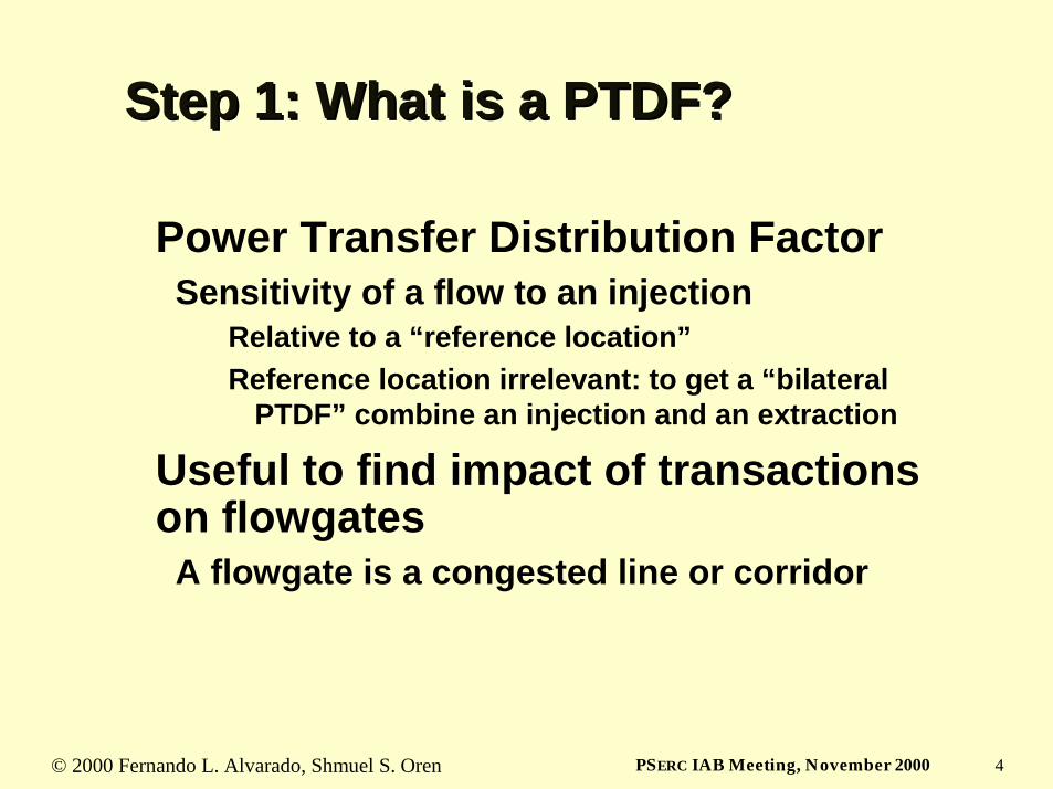
Step 1: What is a PTDF?Step 1: What is a PTDF?
Power Transfer Distribution FactorSensitivity of a flow to an injection
Relative to a “reference location”Reference location irrelevant: to get a “bilateral
PTDF” combine an injection and an extraction
Useful to find impact of transactions on flowgates
A flowgate is a congested line or corridor
© 2000 Fernando L. Alvarado, Shmuel S. Oren 5PSERC IAB Meeting, November 2000
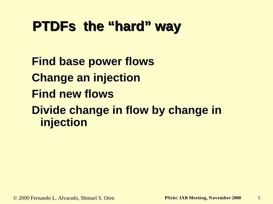
PTDFs the “hard” wayPTDFs the “hard” way
Find base power flowsChange an injectionFind new flowsDivide change in flow by change in
injection
© 2000 Fernando L. Alvarado, Shmuel S. Oren 6PSERC IAB Meeting, November 2000
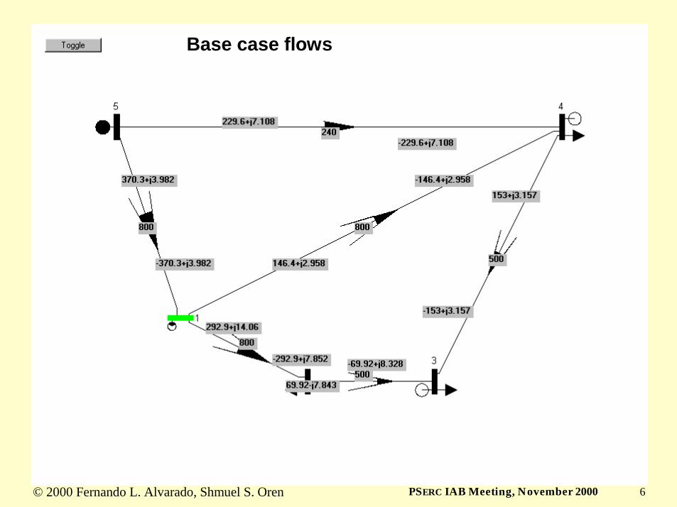
Base case flows
© 2000 Fernando L. Alvarado, Shmuel S. Oren 7PSERC IAB Meeting, November 2000
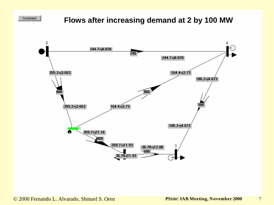
Flows after increasing demand at 2 by 100 MW
© 2000 Fernando L. Alvarado, Shmuel S. Oren 8PSERC IAB Meeting, November 2000
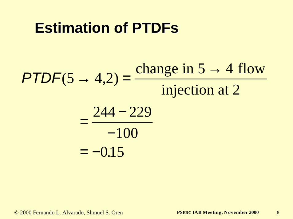
Estimation of PTDFsEstimation of PTDFs
PTDF( , )
.
5 4 2 5 4
244 229100
015
→ = →
= −−
= −
change in flowinjection at 2
© 2000 Fernando L. Alvarado, Shmuel S. Oren 9PSERC IAB Meeting, November 2000
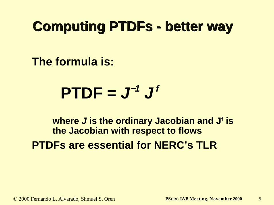
Computing PTDFs Computing PTDFs -- better waybetter way
The formula is:
PTDF = J−−−−1 J f
where J is the ordinary Jacobian and Jf is the Jacobian with respect to flows
PTDFs are essential for NERC’s TLR
© 2000 Fernando L. Alvarado, Shmuel S. Oren 10PSERC IAB Meeting, November 2000
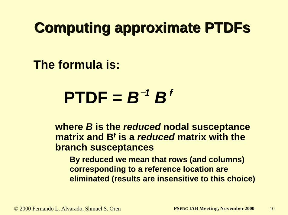
Computing approximate PTDFsComputing approximate PTDFs
The formula is:
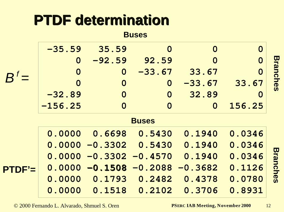
PTDF = B−−−−1 B f
where B is the reduced nodal susceptance matrix and Bf is a reduced matrix with the branch susceptances
By reduced we mean that rows (and columns) corresponding to a reference location are eliminated (results are insensitive to this choice)
© 2000 Fernando L. Alvarado, Shmuel S. Oren 11PSERC IAB Meeting, November 2000
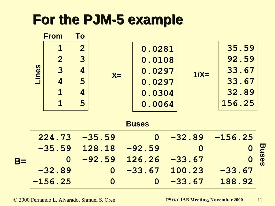
For the PJMFor the PJM--5 example5 example
224.73 -35.59 0 -32.89 -156.25-35.59 128.18 -92.59 0 0
0 -92.59 126.26 -33.67 0-32.89 0 -33.67 100.23 -33.67
-156.25 0 0 -33.67 188.92
B=
X=
0.02810.01080.02970.02970.03040.0064
1/X=
35.5992.5933.6733.6732.89
156.25
1 22 33 44 51 41 5
From ToLi
nes
Buses
Buses
© 2000 Fernando L. Alvarado, Shmuel S. Oren 12PSERC IAB Meeting, November 2000
PTDF determinationPTDF determination
-35.59 35.59 0 0 00 -92.59 92.59 0 00 0 -33.67 33.67 00 0 0 -33.67 33.67
-32.89 0 0 32.89 0-156.25 0 0 0 156.25
B f =
Buses
Branches
0.0000 0.6698 0.5430 0.1940 0.03460.0000 -0.3302 0.5430 0.1940 0.03460.0000 -0.3302 -0.4570 0.1940 0.03460.0000 --0.15080.1508 -0.2088 -0.3682 0.11260.0000 0.1793 0.2482 0.4378 0.07800.0000 0.1518 0.2102 0.3706 0.8931
Branches
Buses
PTDF’=
© 2000 Fernando L. Alvarado, Shmuel S. Oren 13PSERC IAB Meeting, November 2000
Step 2: The “marginal unit”Step 2: The “marginal unit”
With no constraints and no losses, there is one marginal unit
The “next MW” come from the marginal unitWith losses, several marginal units possible
For one congested flowgate, there are at least two marginal units
There must be at least one more marginal unit than there are active constraints
The power for any location may come from more than one of the marginal units
Units on the margin can reduce their output
© 2000 Fernando L. Alvarado, Shmuel S. Oren 14PSERC IAB Meeting, November 2000
Step 3: Nodal spot pricing of energyStep 3: Nodal spot pricing of energy
The nodal spot price is the cheapest way to deliver one MWh to a location, respecting all limits (including contingency limits)
© 2000 Fernando L. Alvarado, Shmuel S. Oren 15PSERC IAB Meeting, November 2000
PTDFs + Constraints + Marginal PTDFs + Constraints + Marginal Units Units ⇒⇒⇒⇒⇒⇒⇒⇒ Spot PricesSpot Prices
Identify constraining conditionsIdentify marginal unitsSolve simplesimple optimization problem
How cheaply can power be delivered to a location from these units respecting all constraints?What is the shadow price (marginal value) of the capacity on the congested flowgates?
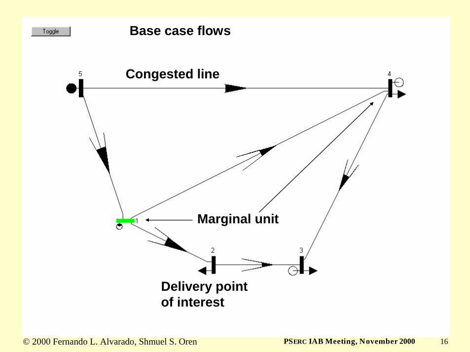
© 2000 Fernando L. Alvarado, Shmuel S. Oren 16PSERC IAB Meeting, November 2000
Base case flows
Marginal unit
Congested line
Delivery pointof interest
© 2000 Fernando L. Alvarado, Shmuel S. Oren 17PSERC IAB Meeting, November 2000
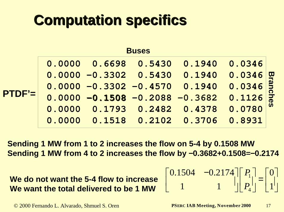
Computation specificsComputation specifics
0.0000 0.6698 0.5430 0.1940 0.03460.0000 -0.3302 0.5430 0.1940 0.03460.0000 -0.3302 -0.4570 0.1940 0.03460.0000 --0.15080.1508 -0.2088 -0.3682 0.11260.0000 0.1793 0.2482 0.4378 0.07800.0000 0.1518 0.2102 0.3706 0.8931
Branches
Buses
PTDF’=
Sending 1 MW from 1 to 2 increases the flow on 5-4 by 0.1508 MWSending 1 MW from 4 to 2 increases the flow by −−−−0.3682+0.1508====−−−−0.2174
We do not want the 5-4 flow to increaseWe want the total delivered to be 1 MW
1
4
0.1504 0.2174 01 1 1
PP
− =
© 2000 Fernando L. Alvarado, Shmuel S. Oren 18PSERC IAB Meeting, November 2000
1
4
0.1504 0.2174 01 1 1
PP
− =
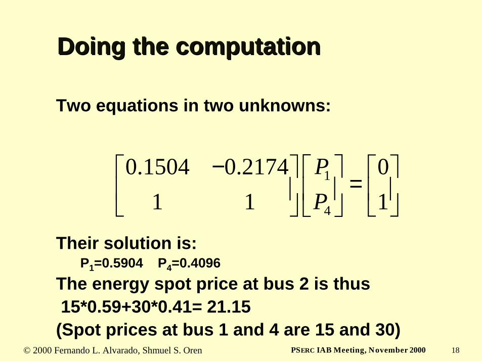
Doing the computationDoing the computation
Two equations in two unknowns:
Their solution is:P1=0.5904 P4=0.4096
The energy spot price at bus 2 is thus15*0.59+30*0.41= 21.15(Spot prices at bus 1 and 4 are 15 and 30)
© 2000 Fernando L. Alvarado, Shmuel S. Oren 19PSERC IAB Meeting, November 2000
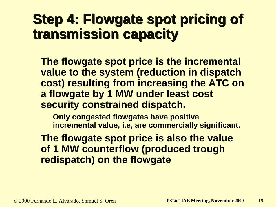
Step 4: Flowgate spot pricing of Step 4: Flowgate spot pricing of transmission capacitytransmission capacity
The flowgate spot price is the incremental value to the system (reduction in dispatch cost) resulting from increasing the ATC on a flowgate by 1 MW under least cost security constrained dispatch.
Only congested flowgates have positive incremental value, i.e, are commercially significant.
The flowgate spot price is also the value of 1 MW counterflow (produced trough redispatch) on the flowgate
© 2000 Fernando L. Alvarado, Shmuel S. Oren 20PSERC IAB Meeting, November 2000
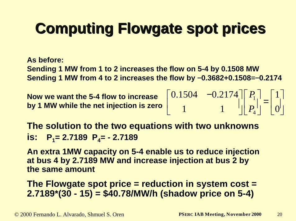
Computing Flowgate spot pricesComputing Flowgate spot prices
As before:Sending 1 MW from 1 to 2 increases the flow on 5-4 by 0.1508 MWSending 1 MW from 4 to 2 increases the flow by −−−−0.3682+0.1508====−−−−0.2174
Now we want the 5-4 flow to increase by 1 MW while the net injection is zero
1
4
0.1504 0.2174 11 1 0
PP
− =
The solution to the two equations with two unknowns is: P1= 2.7189 P4= - 2.7189An extra 1MW capacity on 5-4 enable us to reduce injection at bus 4 by 2.7189 MW and increase injection at bus 2 by the same amount
The Flowgate spot price = reduction in system cost = 2.7189*(30 - 15) = $40.78/MW/h (shadow price on 5-4)
© 2000 Fernando L. Alvarado, Shmuel S. Oren 21PSERC IAB Meeting, November 2000
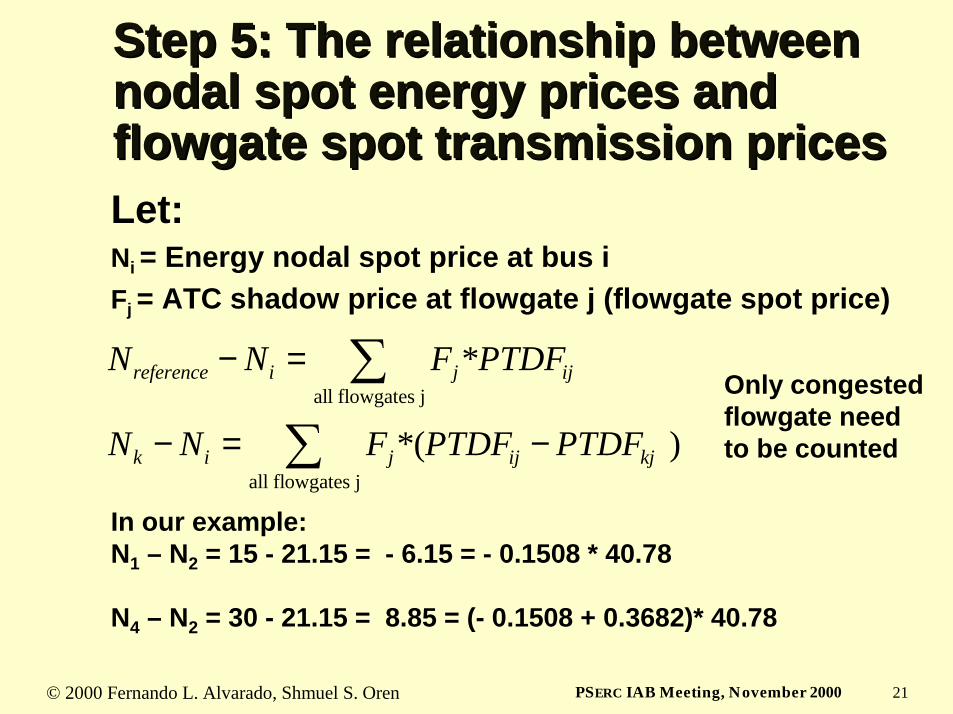
Step 5: The relationship between Step 5: The relationship between nodal spot energy prices and nodal spot energy prices and flowgate spot transmission pricesflowgate spot transmission pricesLet: Ni = Energy nodal spot price at bus iFj = ATC shadow price at flowgate j (flowgate spot price)
all flowgates j
all flowgates j
*
*( )
reference i j ij
k i j ij kj
N N F PTDF
N N F PTDF PTDF
− =
− = −
∑
∑In our example:N1 – N2 = 15 - 21.15 = - 6.15 = - 0.1508 * 40.78
N4 – N2 = 30 - 21.15 = 8.85 = (- 0.1508 + 0.3682)* 40.78
Only congestedflowgate need to be counted
© 2000 Fernando L. Alvarado, Shmuel S. Oren 22PSERC IAB Meeting, November 2000
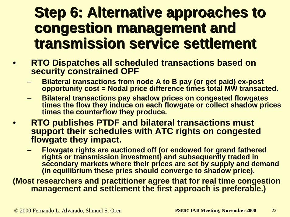
Step 6: Alternative approaches to Step 6: Alternative approaches to congestion management and congestion management and transmission service settlementtransmission service settlement
• RTO Dispatches all scheduled transactions based on security constrained OPF
– Bilateral transactions from node A to B pay (or get paid) ex-post opportunity cost = Nodal price difference times total MW transacted.
– Bilateral transactions pay shadow prices on congested flowgates times the flow they induce on each flowgate or collect shadow prices times the counterflow they produce.
• RTO publishes PTDF and bilateral transactions must support their schedules with ATC rights on congested flowgate they impact.
– Flowgate rights are auctioned off (or endowed for grand fatheredrights or transmission investment) and subsequently traded in secondary markets where their prices are set by supply and demand (in equilibrium these pries should converge to shadow price).
(Most researchers and practitioner agree that for real time congestion management and settlement the first approach is preferable.)

© 2000 Fernando L. Alvarado, Shmuel S. Oren 23PSERC IAB Meeting, November 2000
Tradable Property RightsTradable Property Rights
Purpose: – Facilitates efficient use of scarce resources (Coase)– Mechanism to reward investment– Enable risk management (hedging, forward
markets)Aspects of Property rights:
– Right to financial gain from asset– Right to use asset (weak physical)– Right to exclude others from using the asset
(strong physical)
© 2000 Fernando L. Alvarado, Shmuel S. Oren 24PSERC IAB Meeting, November 2000
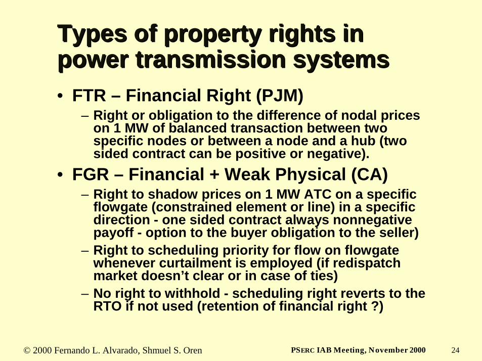
Types of property rights in Types of property rights in power transmission systemspower transmission systems• FTR – Financial Right (PJM)
– Right or obligation to the difference of nodal prices on 1 MW of balanced transaction between two specific nodes or between a node and a hub (two sided contract can be positive or negative).
• FGR – Financial + Weak Physical (CA)– Right to shadow prices on 1 MW ATC on a specific
flowgate (constrained element or line) in a specific direction - one sided contract always nonnegative payoff - option to the buyer obligation to the seller)
– Right to scheduling priority for flow on flowgate whenever curtailment is employed (if redispatch market doesn’t clear or in case of ties)
– No right to withhold - scheduling right reverts to the RTO if not used (retention of financial right ?)
© 2000 Fernando L. Alvarado, Shmuel S. Oren 25PSERC IAB Meeting, November 2000
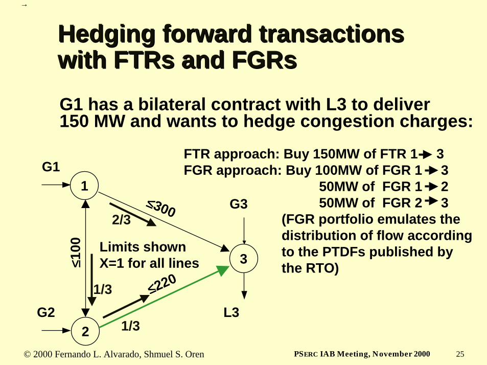
Hedging forward transactions Hedging forward transactions with FTRs and FGRswith FTRs and FGRsG1 has a bilateral contract with L3 to deliver 150 MW and wants to hedge congestion charges:
1
3
2
≤≤≤≤300
≤≤≤≤220
≤≤ ≤≤100 Limits shown
X=1 for all lines
G1
G2 L3
FTR approach: Buy 150MW of FTR 1 3FGR approach: Buy 100MW of FGR 1 3
50MW of FGR 1 250MW of FGR 2 3
(FGR portfolio emulates the distribution of flow according to the PTDFs published by the RTO)
→
2/3
1/3
1/3
G3
© 2000 Fernando L. Alvarado, Shmuel S. Oren 26PSERC IAB Meeting, November 2000
Real time settlementsReal time settlementsSuppose real time dispatch is based on security constrained
OPF and the flow constraint on link 2 3 with corresponding shadow price F23 (shadow prices on uncongested links are zero) and nodal prices N1 , N2, N3
Nodal pricing based congestion charges paid by the generator for the 150MW transaction from node 1 to 3 are 150*(N3- N1)
Settlement for 150MW FTR 1 3 paid to the generator is 100*(N3- N1)
Settlement for 50MW FGR 2 3 is 50* F23.. But N3- N1=1/3* F23 (relation of nodal and shadow prices)
Both the FTR and FGR settlements offset the real time congestion charges (full hedging)
© 2000 Fernando L. Alvarado, Shmuel S. Oren 27PSERC IAB Meeting, November 2000
So what is the difference?So what is the difference?
• FTRs guarantee a perfect hedge– Insurance against congestion on flowgates– Insurance against changes in PTDFs– Insurance against changes in ATC on flowgate– Solvency conditions necessitates limiting the FTR
offering• FGRs only provides insurance against
congestion on flowgates– Holder is responsible to maintain proper mix– PTDF tracking services or insurance against deviation
can be offered as a service by private commercial entities– Socialization of changes in congestion cost due to PTDF
changes proposed (e.g. MISO) but is a bad idea
© 2000 Fernando L. Alvarado, Shmuel S. Oren 28PSERC IAB Meeting, November 2000
Issuing and trading FTRsIssuing and trading FTRs• FTRs representing financial property rights to the
transmission system must be issued centrally by the RTO (Speculative FTRs “off track betting” can be issued by anyone but have no physical cover)
• To insure that congestion revenues can cover FTR settlements FTRs must meet a “simultaneous feasibility condition”
• The FTR “operating point” corresponding to simultaneous bilateral schedules replicating all outstanding FTRs must meet all security and flow constraints.
• In an FTR auction (PJM) bidders submit bids for specific FTRs, RTO selects winning bids by treating FTR bids as proposed schedules using a security constraint OPF that maximizes FTR revenue
© 2000 Fernando L. Alvarado, Shmuel S. Oren 29PSERC IAB Meeting, November 2000
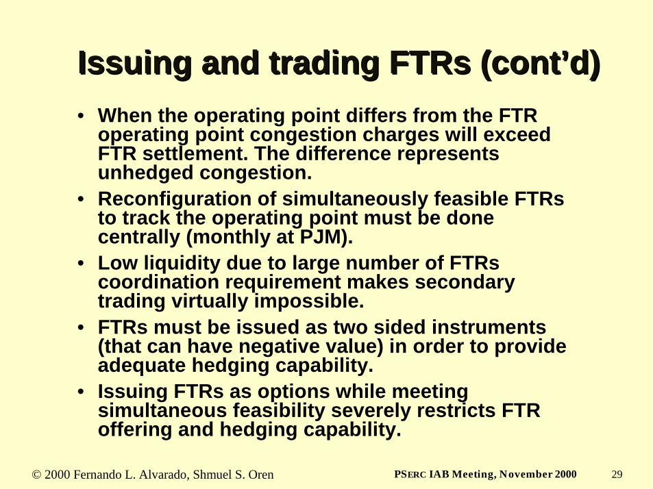
Issuing and trading FTRs (cont’d)Issuing and trading FTRs (cont’d)• When the operating point differs from the FTR
operating point congestion charges will exceed FTR settlement. The difference represents unhedged congestion.
• Reconfiguration of simultaneously feasible FTRs to track the operating point must be done centrally (monthly at PJM).
• Low liquidity due to large number of FTRs coordination requirement makes secondary trading virtually impossible.
• FTRs must be issued as two sided instruments (that can have negative value) in order to provide adequate hedging capability.
• Issuing FTRs as options while meeting simultaneous feasibility severely restricts FTR offering and hedging capability.
© 2000 Fernando L. Alvarado, Shmuel S. Oren 30PSERC IAB Meeting, November 2000
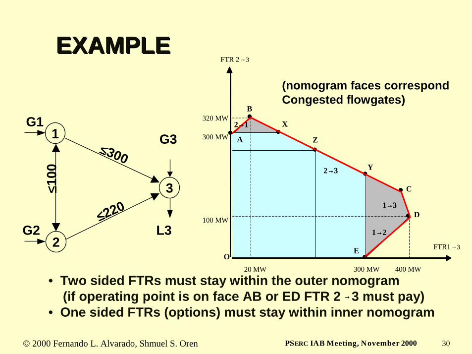
EXAMPLEEXAMPLE
1
3
2
≤≤≤≤300
≤≤≤≤220
≤≤ ≤≤100
G1
G2 L3
G3
• Two sided FTRs must stay within the outer nomogram(if operating point is on face AB or ED FTR 2 3 must pay)
• One sided FTRs (options) must stay within inner nomogram→→→→
300 MW
300 MW
400 MW
100 MW
320 MW
20 MW
FTR 2→3
FTR1→3
•
•
•
•
•
Y
Z
X
•
B
C
D
E
A•
•
O
2→→→→1
2→→→→3
1→→→→3
1→→→→2
(nomogram faces correspond Congested flowgates)
© 2000 Fernando L. Alvarado, Shmuel S. Oren 31PSERC IAB Meeting, November 2000
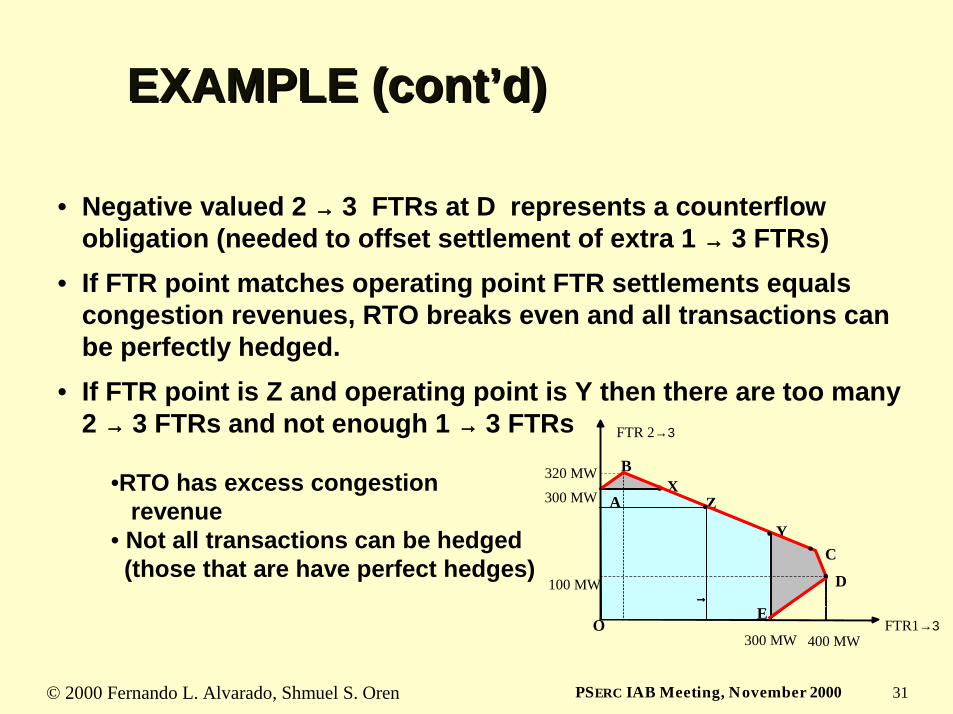
EXAMPLE (cont’d)EXAMPLE (cont’d)
• Negative valued 2 →→→→ 3 FTRs at D represents a counterflow obligation (needed to offset settlement of extra 1 →→→→ 3 FTRs)
• If FTR point matches operating point FTR settlements equals congestion revenues, RTO breaks even and all transactions can be perfectly hedged.
• If FTR point is Z and operating point is Y then there are too many 2 →→→→ 3 FTRs and not enough 1 →→→→ 3 FTRs
•RTO has excess congestionrevenue
• Not all transactions can be hedged (those that are have perfect hedges)
300 MW 400 MW
300 MW
100 MW
320 MW
FTR1→3
•
Y
ZX
B
C
D
E
A
O
• •
•
•
FTR 2→3
→→→→
© 2000 Fernando L. Alvarado, Shmuel S. Oren 32PSERC IAB Meeting, November 2000
• RTO auctions FGRs (financial with or without scheduling priority) as property rights to the directional flowgates’ physical capacity
• Only commercially significant flowgates (those likely to congest) need to be included in auction
• FGRs are issued as options since settlement (based on shadow prices) can only be positive or zero
• Number of FGRs on each flowgate determined independently of others (no simultaneous feasibility condition)
• RTO publishes current PTDFs informing traders FGR mix needed to hedge point to point transactions
Issuing and trading FGRsIssuing and trading FGRs
© 2000 Fernando L. Alvarado, Shmuel S. Oren 33PSERC IAB Meeting, November 2000
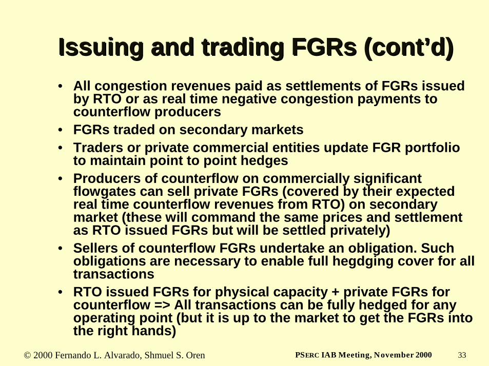
Issuing and trading FGRs (cont’d)Issuing and trading FGRs (cont’d)• All congestion revenues paid as settlements of FGRs issued
by RTO or as real time negative congestion payments to counterflow producers
• FGRs traded on secondary markets• Traders or private commercial entities update FGR portfolio
to maintain point to point hedges• Producers of counterflow on commercially significant
flowgates can sell private FGRs (covered by their expected real time counterflow revenues from RTO) on secondary market (these will command the same prices and settlement as RTO issued FGRs but will be settled privately)
• Sellers of counterflow FGRs undertake an obligation. Such obligations are necessary to enable full hegdging cover for all transactions
• RTO issued FGRs for physical capacity + private FGRs for counterflow => All transactions can be fully hedged for any operating point (but it is up to the market to get the FGRs intothe right hands)
© 2000 Fernando L. Alvarado, Shmuel S. Oren 34PSERC IAB Meeting, November 2000
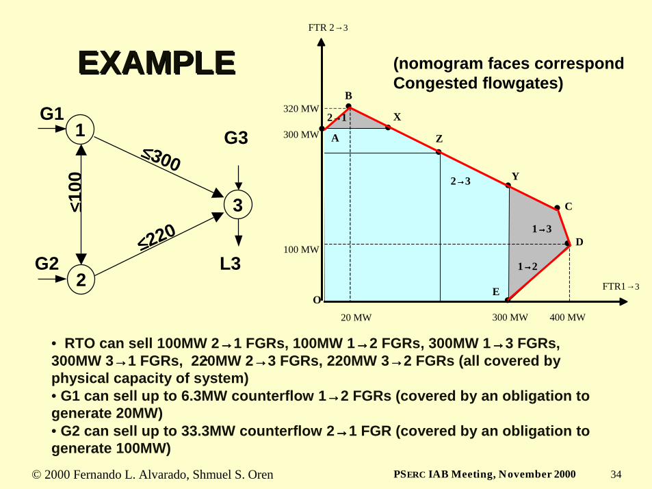
EXAMPLEEXAMPLE
• RTO can sell 100MW 2→→→→1 FGRs, 100MW 1→→→→2 FGRs, 300MW 1→→→→3 FGRs, 300MW 3→→→→1 FGRs, 220MW 2→→→→3 FGRs, 220MW 3→→→→2 FGRs (all covered by physical capacity of system)• G1 can sell up to 6.3MW counterflow 1→→→→2 FGRs (covered by an obligation to generate 20MW) • G2 can sell up to 33.3MW counterflow 2→→→→1 FGR (covered by an obligation to generate 100MW)
1
3
2
≤≤≤≤300
≤≤≤≤220
≤≤ ≤≤100
G1
G2 L3
G3
300 MW
300 MW
400 MW
100 MW
320 MW
20 MW
FTR 2→3
FTR1→3
•
•
•
•
•
Y
Z
X
•
B
C
D
E
A•
•
O
2→→→→1
2→→→→3
1→→→→3
1→→→→2
(nomogram faces correspond Congested flowgates)
→→→→
© 2000 Fernando L. Alvarado, Shmuel S. Oren 35PSERC IAB Meeting, November 2000
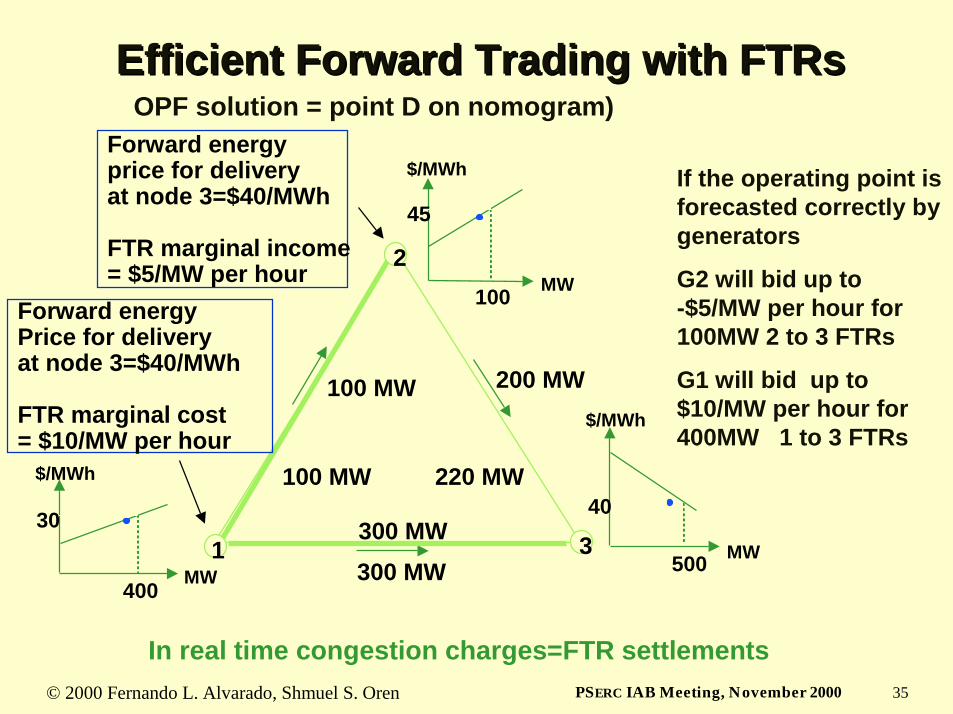
Efficient Forward Trading with FTRsEfficient Forward Trading with FTRs
3
100 MW 200 MW
300 MW
100 MW 220 MW
300 MW
100
45
MW
$/MWh
400
30
MW
$/MWh
500
40
MW
$/MWh
2
1
Forward energy price for deliveryat node 3=$40/MWh
FTR marginal income = $5/MW per hour
Forward energy Price for delivery at node 3=$40/MWh
FTR marginal cost= $10/MW per hour
If the operating point is forecasted correctly by generators
G2 will bid up to -$5/MW per hour for 100MW 2 to 3 FTRs
G1 will bid up to $10/MW per hour for 400MW 1 to 3 FTRs
OPF solution = point D on nomogram)
In real time congestion charges=FTR settlements
© 2000 Fernando L. Alvarado, Shmuel S. Oren 36PSERC IAB Meeting, November 2000
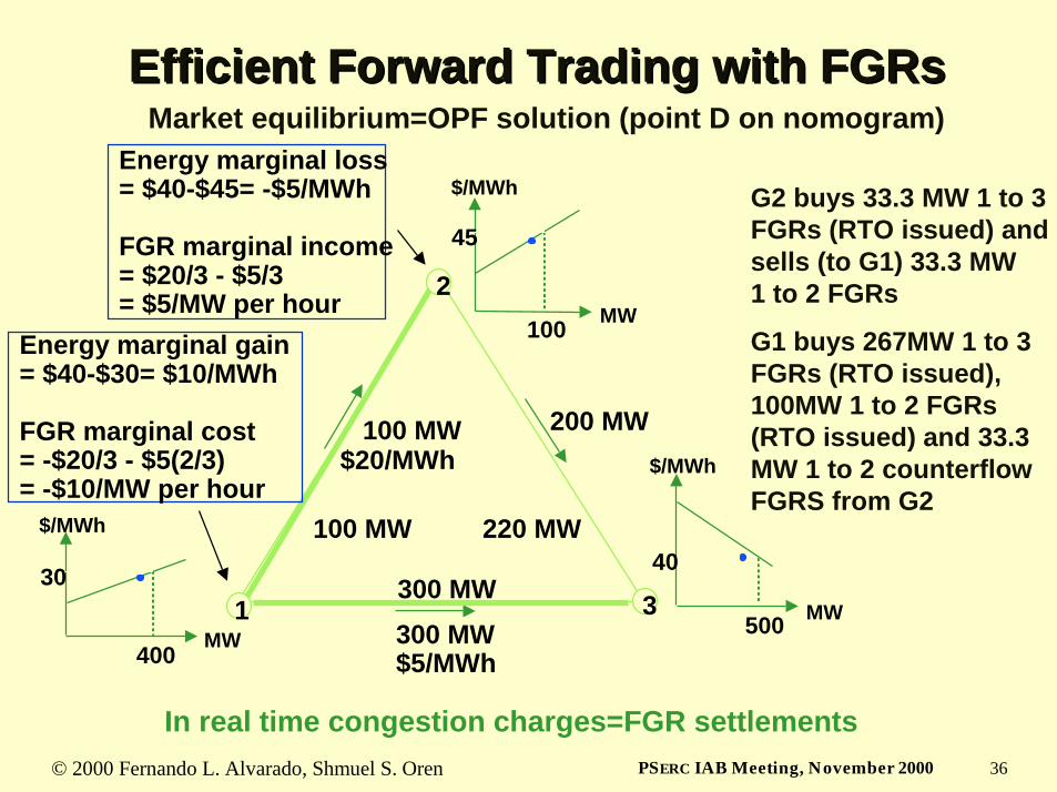
Efficient Forward Trading with FGRsEfficient Forward Trading with FGRs
3
100 MW 200 MW
300 MW$5/MWh
$20/MWh
100 MW 220 MW
300 MW
100
45
MW
$/MWh
400
30
MW
$/MWh
500
40
MW
$/MWh
2
1
Energy marginal loss = $40-$45= -$5/MWh
FGR marginal income = $20/3 - $5/3 = $5/MW per hour
Energy marginal gain = $40-$30= $10/MWh
FGR marginal cost= -$20/3 - $5(2/3)= -$10/MW per hour
G2 buys 33.3 MW 1 to 3 FGRs (RTO issued) and sells (to G1) 33.3 MW 1 to 2 FGRs
G1 buys 267MW 1 to 3 FGRs (RTO issued), 100MW 1 to 2 FGRs (RTO issued) and 33.3 MW 1 to 2 counterflow FGRS from G2
Market equilibrium=OPF solution (point D on nomogram)
In real time congestion charges=FGR settlements
© 2000 Fernando L. Alvarado, Shmuel S. Oren 37PSERC IAB Meeting, November 2000
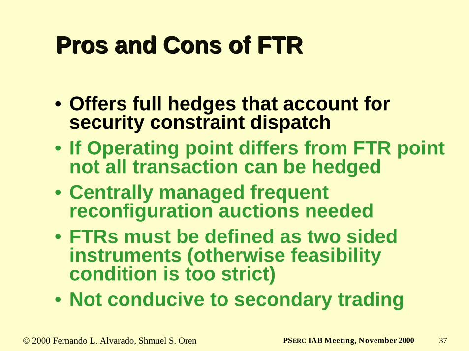
Pros and Cons of FTRPros and Cons of FTR
• Offers full hedges that account for security constraint dispatch
• If Operating point differs from FTR point not all transaction can be hedged
• Centrally managed frequent reconfiguration auctions needed
• FTRs must be defined as two sided instruments (otherwise feasibility condition is too strict)
• Not conducive to secondary trading
© 2000 Fernando L. Alvarado, Shmuel S. Oren 38PSERC IAB Meeting, November 2000
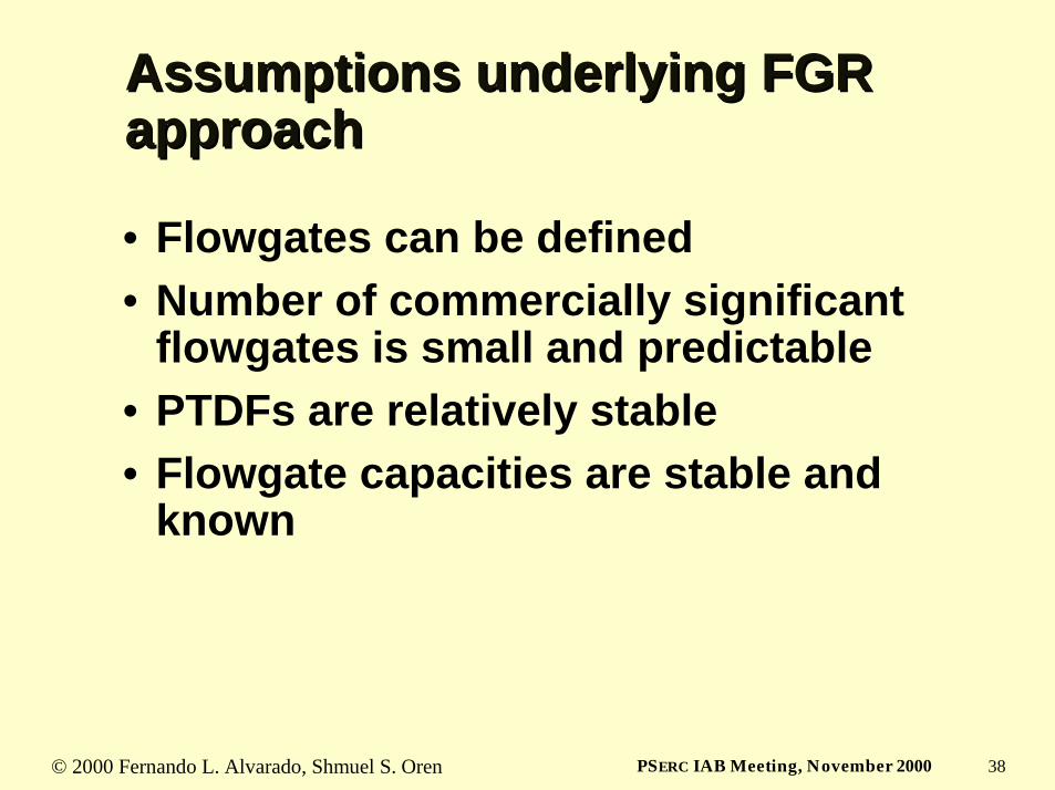
Assumptions underlying FGR Assumptions underlying FGR approachapproach
• Flowgates can be defined • Number of commercially significant
flowgates is small and predictable• PTDFs are relatively stable • Flowgate capacities are stable and
known
© 2000 Fernando L. Alvarado, Shmuel S. Oren 39PSERC IAB Meeting, November 2000
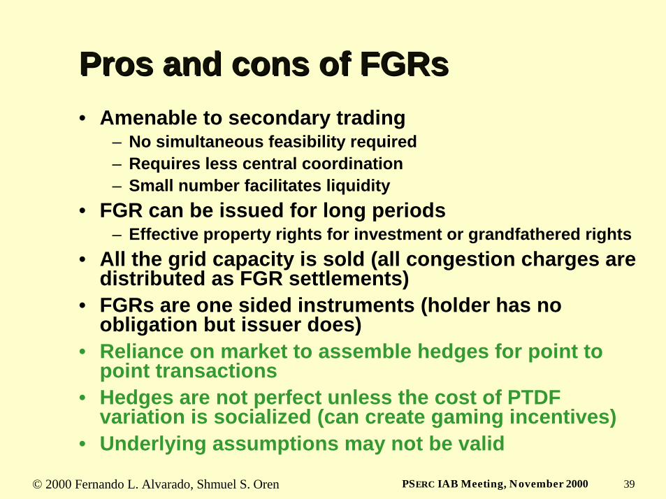
Pros and cons of FGRsPros and cons of FGRs• Amenable to secondary trading
– No simultaneous feasibility required– Requires less central coordination– Small number facilitates liquidity
• FGR can be issued for long periods – Effective property rights for investment or grandfathered rights
• All the grid capacity is sold (all congestion charges are distributed as FGR settlements)
• FGRs are one sided instruments (holder has no obligation but issuer does)
• Reliance on market to assemble hedges for point to point transactions
• Hedges are not perfect unless the cost of PTDF variation is socialized (can create gaming incentives)
• Underlying assumptions may not be valid
© 2000 Fernando L. Alvarado, Shmuel S. Oren 40PSERC IAB Meeting, November 2000
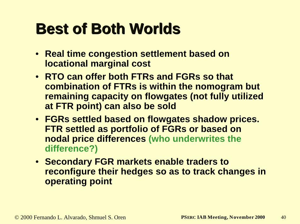
Best of Both WorldsBest of Both Worlds• Real time congestion settlement based on
locational marginal cost• RTO can offer both FTRs and FGRs so that
combination of FTRs is within the nomogram but remaining capacity on flowgates (not fully utilized at FTR point) can also be sold
• FGRs settled based on flowgates shadow prices. FTR settled as portfolio of FGRs or based on nodal price differences (who underwrites the difference?)
• Secondary FGR markets enable traders to reconfigure their hedges so as to track changes in operating point